Proxy-based Item Representation for Attribute and Context-aware Recommendation

Abstract.

Neural network approaches in recommender systems have shown remarkable success by representing a large set of items as a learnable vector embedding table. However, infrequent items may suffer from inadequate training opportunities, making it difficult to learn meaningful representations. We examine that in attribute and context-aware settings, the poorly learned embeddings of infrequent items impair the recommendation accuracy. To address such an issue, we propose a proxy-based item representation that allows each item to be expressed as a weighted sum of learnable proxy embeddings. Here, the proxy weight is determined by the attributes and context of each item and may incorporate bias terms in case of frequent items to further reflect collaborative signals. The proxy-based method calculates the item representations compositionally, ensuring each representation resides inside a well-trained simplex and, thus, acquires guaranteed quality. Additionally, that the proxy embeddings are shared across all items allows the infrequent items to borrow training signals of frequent items in a unified model structure and end-to-end manner. Our proposed method is a plug-and-play model that can replace the item encoding layer of any neural network-based recommendation model, while consistently improving the recommendation performance with much smaller parameter usage. Experiments conducted on real-world recommendation benchmark datasets demonstrate that our proposed model outperforms state-of-the-art models in terms of recommendation accuracy by up to 17% while using only 10% of the parameters.

1. Introduction

Recommender systems have evolved from collaborative filtering (CF) (Sarwar et al., 2001) to machine learning (Ning and Karypis, 2011; Rendle, 2010; Guo et al., 2017) and deep learning-based models (Batmaz et al., 2019; Wang et al., 2019). In model-based CF (Koren et al., 2009), users and items are represented as latent vectors via learnable embedding matrix, which is implemented as a full look-up table, where each row corresponds to a unique user or item vector. Such vector representation approach can transform the recommendation problem into a set of vector arithmetic, assuming that the latent vectors are well-trained through the training data distribution (Tran et al., 2019). To train the representations effectively and achieve higher recommendation performance, recent studies have introduced deep learning-based models (He et al., 2017; Xue et al., 2017; Vaswani et al., 2017) and sequential recommendation models (Quadrana et al., 2017; Kang and McAuley, 2018; Sun et al., 2019; Petrov and Macdonald, 2022b) as well as attribute (He and McAuley, 2016; Zhou et al., 2020) and context-aware (Guo et al., 2017; Rashed et al., 2022) models.

The concept of item embedding matrix also appears in the Natural Language Processing (NLP) field to train the distributional semantics of words (Mikolov et al., 2013). However, in contrast to the data distributions in NLP, recommendation datasets exhibit distinct and unique characteristics, which incur two significant limitations that need to be addressed. Firstly, the item frequency in recommendation datasets follows a long-tail distribution (Yin et al., 2012). The item embedding matrix, which is unaware of such data distribution, cannot accurately reflect the proper training signals for the infrequent items (Naumov et al., 2021; Movshovitz-Attias et al., 2017), leading to degraded recommendation performance (Ardalani et al., 2022). Secondly, the number of items may increase indefinitely. For a real-world recommendation scenario, a large set of new items is consistently added to the system (Pfadler et al., 2020; Covington et al., 2016) and the item embedding matrix, where most of the model parameters are stored (Ardalani et al., 2022), must scale up accordingly to accommodate them. For these problems being the case, it is necessary to devise a new methodology that can effectively replace the item embedding matrix and resolve such limitations.

We further investigate the problem of infrequent item embeddings thoroughly. First of all, during the training process of a recommendation model, items appear in three different scenarios: a user profile that is represented as a list of interacted items, a target item for the system to predict, and a set of negative items that the user has not interacted obtained via negative sampling. It is evident that the parameter update for a specific item embedding, except for that of negative sampled items, is directly proportional to the item’s occurrence frequency. Consequently, infrequent items do not receive as many training opportunities as frequent items do and, thus, their embeddings hardly converge to their optimal states throughout the training. We have conducted an empirical analysis of such phenomena under attribute and context-aware settings (Kang and McAuley, 2018; Rashed et al., 2022). Specifically, we have replaced a portion of infrequent items with a shared unknown token and measured the model performance. In Table 1, when the infrequent items are replaced by the unknown token, which can be seen as a removal process, the recommendation accuracy in terms of NDCG@10 increases. Such result clearly demonstrates that the poorly learned infrequent item embeddings harm the overall performance as mentioned earlier. However, such improvement comes at the cost of losing global coverage of recommended items, which accounts for item diversity, and highlights that the insufficient training signals for infrequent items need to be addressed.

Previous studies that aim to resolve the aforementioned issues can be divided into two branches. Firstly, to mitigate the negative impact of infrequent item embeddings on the model performance while reducing the parameter usage, (Chen et al., 2023) employed a shared embedding through clustering and (Naumov et al., 2021) reduced the embedding dimension of infrequent items. However, these methods are not suitable for datasets where content information (i.e., item attributes and contexts) is crucial (e.g., Fashion domain, showing large performance gap when content information is not utilized). Secondly, (Wei et al., 2021; Zhu et al., 2021; Chen et al., 2022b) proposed methods that allow the embeddings of infrequent items to mimic those of frequent items using their content information. However, they have separate model structures (e.g., mimicking network) and learning strategies (e.g., warm-up stage), which makes it difficult to train in an end-to-end fashion, resulting in unstable hyper-parameter tuning.

In this paper, we propose a novel proxy-based item representation model that represents each item as a weighted sum of learnable proxy embeddings by leveraging content information, while incorporating the learning process of both frequent and infrequent items into a single framework in an end-to-end manner. Generally, a proxy refers to a model or a vector learned in place of the original training objective to improve the training efficiency or performance in deep learning (Caron et al., 2020; Movshovitz-Attias et al., 2017). We reduce the item embedding matrix into two linearly combinable components: the proxy weighting network and the proxy embedding. Our model represents an item as the weighted sum of learnable proxy embeddings, where the weights are primarily determined by content information. As opposed to the infrequent items, frequent items possess abundant collaborative signals. To further incorporate such signals whenever available, we add learnable bias terms to the proxy weights. By such means, the model can learn hybrid collaborative signals in a single representation space that encompasses not only item ID-to-ID but also ID-to-content and content-to-content relations.

The core concept of our proposed model is illustrated in Figure 1. We apply a softmax function on the proxy weights to enforce the weights sum up to 1. This approach ensures each item representation resides inside a simplex where vertices are well-trained proxy embeddings. Moreover, since the gradient is formed in a unit of proxy embeddings that are shared across all items, the training becomes stable and fast while allowing infrequent items to borrow the training signal of frequent items. Additionally, that newly added item can be computed compositionally via proxy embeddings based on their content information prevents the indefinite increase of parameters, resulting in parameter efficiency. As a result, our method alleviates the inadequate parameter updates of those items that exist in long-tail distribution, leading to performance improvement with much smaller parameter usage.

We conduct experiments on real-world recommendation benchmark datasets, namely Amazon Review datasets (McAuley et al., 2015) and MovieLens dataset. Each dataset has its distinct data distribution and item attributes, along with context and sequential information. Our proposed method is a plug-and-play model that can replace the item encoding layer of any neural network-based recommendation model, and the experimental results show that leveraging our model consistently improves the performance across all datasets.

Table 1. Performance and diversity comparison of infrequent item removal ratio on Fashion

Model	Removal	#params (M)	NDCG@10	Diversity
	0%	45.8	37.9%	15.0%
	25%	35.1	39.1%	14.9%
SASRec++	50%	24.5	39.2%	14.8%
	75%	13.9	40.2%	13.1%
	90%	7.5	41.6%	11.6%
	0%	25.1	42.6%	16.2%
	25%	19.7	42.5%	15.3%
with PIR	50%	14.4	42.5%	16.2%
	75%	9.1	42.4%	16.2%
	90%	5.9	42.4%	16.0%

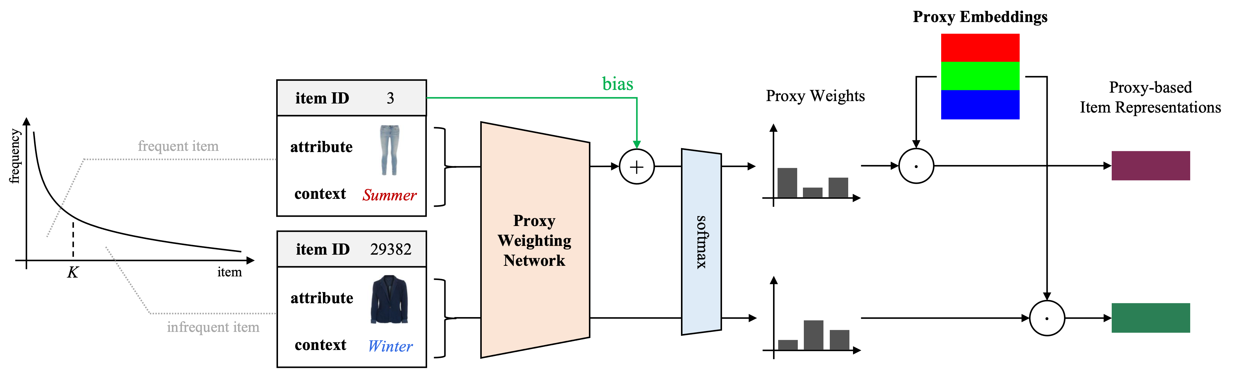
Figure 1. Proxy-based item representation model. Items are represented as a weighted sum of learnable proxy embeddings.

2. Related Work

Our model is inspired by three research branches: attribute and context-aware sequential recommendation (ACSR) models (Zhou et al., 2020; Petrov and Macdonald, 2022a, b; Chen et al., 2022a), parameter-efficient recommendation models (Naumov et al., 2021; Kang et al., 2021; Liu et al., 2021), and proxy learning models (Kim et al., 2020; Cho et al., 2021a) involving clustering techniques in self-supervised learning (Caron et al., 2020; Li et al., 2021b).

The most important feature in the recommendation is the user-item interaction history. However, in certain datasets where interaction data is sparse or item attributes are crucial, leveraging content and contextual information becomes vital (Guo et al., 2017; Zhou et al., 2020; Wei et al., 2021; Seol et al., 2022). For example, the current state-of-the-art ACSR model CARCA (Rashed et al., 2022) achieves a performance increase of up to 50% in terms of recommendation accuracy when compared to other baseline models that do not reflect all of the following: the attribute, the context, or the sequential information. Furthermore, in the cold-start scenarios where the interaction data are extremely rare, (Wei et al., 2021; Zhu et al., 2021; Chen et al., 2022b) proposed two-structured methods that aim to mimic the embeddings of frequent items by employing content information to boost model performance.

To address the enormous training parameter issue (Ardalani et al., 2022), studies for parameter-efficient recommendation models have been conducted recently (Kang et al., 2021; Naumov et al., 2021; Ardalani et al., 2022; Liu et al., 2021; Yan et al., 2021; Zhao et al., 2020). Most studies focus on devising new methodologies to encode each item into a promising vector representation with fewer parameters (Kang et al., 2021; Naumov et al., 2021; Zhao et al., 2020; Chen et al., 2023) or reduce the model size without hurting the performance (Shen et al., 2021; Yan et al., 2021). In the mixed-dimension model (Naumov et al., 2021), the item embedding matrix is split into two parts: frequent and infrequent items, where the embeddings of the latter are factorized into low-rank matrices. Such method has the potential to alleviate the negative impact of infrequent item embeddings on the model performance while reducing the overall parameter usage. In the hash-based method (Kang et al., 2021), the embedding matrix is compressed through multiple hash functions, representing the item embeddings as the combination of hash values. The clustering-based method of (Chen et al., 2023) also aims to resolve inherent issues of the embedding matrix by using the shared embeddings. However, such methods does not reflect essential recommendation properties, such as the attributes of items and the recommendation contexts, limiting performance improvement in certain datasets that heavily resort to item content information (e.g., Fashion domain).

The concept of utilizing proxies has been applied and verified in many studies from various fields with similar motivations: infrequently occurring objects borrowing the training signals from frequently occurring objects. Among numerous recommendation models, ProxySR (Cho et al., 2021a) employs user proxy embeddings to augment information for item sequences with a relatively short length in a session-based setting. However, ProxySR explicitly selects one proxy user at a time, which is very different from our proposed model that represents items by combining multiple proxy item embeddings. Concretely, proxies in ProxySR represent prototypical users, while proxies in our model represents cluster centroids of items that serve as necessary components for item representations. Despite such differences, ProxySR successfully demonstrates that the proxy embeddings serve as an external memory (Dong et al., 2020) of collaborative signals (Li et al., 2021a; Fan et al., 2021) and provide a performance improvement.

In computer vision, proxies are also utilized as cluster centroids to improve training efficiency and performance in contrastive learning, namely self-supervised learning (Caron et al., 2020, 2021; Li et al., 2021b; Zhang et al., 2021; Cho et al., 2021b) and metric learning for image retrieval (Wieczorek et al., 2021; Movshovitz-Attias et al., 2017; Kim et al., 2020; Yao et al., 2022). Contrastive learning involves positive and negative sampling, where the complexity of image pairs or triplets becomes enormous (Kim et al., 2020). This leads to inconsistent parameter updates since some positive samples may starve by chance. To address such problem, training is performed between proxies rather than image samples. In this setting, a proxy represents a centroid of an unsupervised cluster or a representative vector of a supervised labeled group. The individual images are then trained via their corresponding proxy. Since the number of proxies is much smaller than the number of images, the network converges faster, and the training becomes more stable while improving the overall performance (Kim et al., 2020). Regarding the recommendation, the infrequent items often undergo insufficient parameter updates, corresponding to the aforementioned inconsistent parameter update of positive samples in the contrastive learning. Therefore, employing proxies that behave similarly to cluster centroids can alleviate such training opportunity starvation of infrequent items.

3. Model

3.1. Problem Definition

Let $U$ and $I$ be the set of all users and all items, respectively. The user item sequence $S_{u}$ of a user $u\in U$ is defined as $S_{u}=(i_{1},i_{2},...,i_{|S_{u}|})$ where $1\leq t\leq|S_{u}|$ and $i_{t}\in I$. We denote a subsequence that uses only the first $t^{\prime}$ items as $S_{u,(t\leq t^{\prime})}$. We define negative items as $I_{u}^{-}=I\setminus I_{u}^{+}$ where $I_{u}^{+}$ is a set of items constituting $S_{u}$. The goal of sequential recommendation (SR) is to predict subsequent items with a given user item sequence (Kang and McAuley, 2018). For every $u\in U$ and each $1\leq t^{\prime}\leq|S_{u}|-1$, the objective is to maximize $P(i_{t^{\prime}+1}|S_{u,(t\leq t^{\prime})})$, when compared to negative items $N_{u}=\{i_{j}^{-}\}_{j=1}^{|N_{u}|}$ that are randomly sampled from $I_{u}^{-}$. We assume that each item has auxiliary information in addition to its interaction history, which is referred to as item attributes. The item attributes exist in various forms, such as images, titles, descriptions, keyword tags, etc. Here, we assume that preprocessing for attributes is done, and we can use it as a $d_{\text{A}}$-dimensional vector $f_{i_{t}}$ for the item $i_{t}$. Meanwhile, a context is the contextual information, generally meaning time, place, situation, etc., that can affect the preference independently of users and items. Similar to attributes, we assume that the context is preprocessed as a $d_{\text{C}}$-dimensional vector $c_{t}$. We extend SR into attribute and context-aware sequential recommendation (ACSR) as follows: maximize $P(i_{t^{\prime}+1}|S_{u,(t\leq t^{\prime})}^{\text{AC}},c_{t^{\prime}+1})$ where $S_{u}^{\text{AC}}=\{(i_{t},f_{i_{t}},c_{t})|1\leq t\leq|S_{u}^{\text{AC}}|\}$.

3.2. Background

The general architecture of an ACSR model can be divided into three parts: the item encoding layer, the sequence encoding blocks, and the item scoring layer. We explain each part based on the design of CARCA (Rashed et al., 2022), where it has (1) a strong item encoding layer that utilizes item attributes and contexts, (2) self-attention-based sequence encoding blocks, and (3) a state-of-the-art item scoring layer using a cross-attention.

3.2.1. Item Encoding Layer

The main function of this layer is to extract the item vector $v_{i_{t}}\in\mathbb{R}^{d}$ given the input $(i_{t},f_{i_{t}},c_{t})$, where $d$ denotes the latent dimension. First, the individual item embedding for the item $i_{t}$ is assigned as $\text{IE}_{i_{t}}$, from the full-item look-up table $\text{IE}\in\mathbb{R}^{|I|\times d_{\text{IE}}}$, where $d_{\text{IE}}$ denotes the dimension of the item embedding. These three vectors $(\text{IE}_{i_{t}},f_{i_{t}},c_{t})$ are then passed to a shallow neural network to obtain the final item vector:

(1) $$z_{i_{t}}=\sigma^{\text{AC}}(\text{cat}_{\text{col}}(f_{i_{t}},c_{t})W^{\text{AC}}+b^{\text{AC}}),$$

(2) $$v_{i_{t}}=\sigma^{\text{item}}(\text{cat}_{\text{col}}(\text{IE}_{i_{t}},z_{i_{t}})W^{\text{item}}+b^{\text{item}}),$$

where $W^{\text{AC}}\in\mathbb{R}^{(d_{A}+d_{\text{C}})\times d_{\text{AC}}}$, $b^{\text{AC}}\in\mathbb{R}^{d_{\text{AC}}}$, $W^{\text{item}}\in\mathbb{R}^{(d_{\text{IE}}+d_{\text{AC}})\times d}$ , $b^{\text{item}}\in\mathbb{R}^{d}$ are weights and biases for corresponding network, $\sigma^{\text{AC}}$, $\sigma^{\text{item}}$ are activation functions, and $\text{cat}_{\text{col}}$ denotes the column-wise vector concatenation.

3.2.2. Sequence Encoding Blocks

With the advent of self-attention blocks, the sequence encoding blocks have been commonly implemented with Transformer (Vaswani et al., 2017) architecture that is superior in terms of both performance and computational efficiency to that of the past, namely RNN or CNN-based methods (Quadrana et al., 2017; Kang and McAuley, 2018). An attention (Attn) is defined as follows: for three given sequences of vectors $Q\in\mathbb{R}^{L_{Q}\times d_{Q}}$, $K\in\mathbb{R}^{L_{K}\times d_{K}}$, $V\in\mathbb{R}^{L_{V}\times d_{V}}$,

(3) $$\text{Attn}(Q,K,V)=\text{softmax}\left((QK^{\top})/\sqrt{d_{QK}}\right)V,$$

where $d_{Q}=d_{K}=d_{QK}$ and $L_{K}=L_{V}=L_{KV}$. Given the number of heads $H$ that is the divisor of $d_{Q}$, $d_{K}$, $d_{V}$, we can create separate linear projection layers so that each head can handle different representations, often referred multi-head attention (MHA):

(4) $$\text{MHA}(Q,K,V)=\text{cat}_{\text{col}}\left(\left[\text{Attn}(QW_{h}^{Q},KW_{h}^{K},VW_{h}^{V})\right]_{h=1}^{H}\right),$$

where $W_{h}^{Q}\in\mathbb{R}^{d_{Q}\times d_{Q}/H}$, $W_{h}^{K}\in\mathbb{R}^{d_{K}\times d_{K}/H}$, $W_{h}^{V}\in\mathbb{R}^{d_{V}\times d_{V}/H}$. The self-attention assumes that $Q$, $K$, and $V$ are the same, and it is used to encode the complex information of the input sequence. In our problem setting, we apply self-attention to item vectors $V_{u}=[v_{i_{1}}^{\top},v_{i_{2}}^{\top},...,v_{i_{t^{\prime}}}^{\top}]^{\top}\in\mathbb{R}^{|S_{u,(t\leq t^{\prime})}^{\text{AC}}|\times d}$:

(5) $$\hat{V}_{u}=\text{MHA}(V_{u},V_{u},V_{u}).$$

Following the architecture of Transformer, the results above are passed to a two-layered point-wise feed-forward network (PWFF), where it is defined as follows: for a matrix $X\in\mathbb{R}^{L_{X}\times d_{X}}$ denoting a set of vectors,

(6) $$\text{PWFF}(X)=\text{cat}_{\text{row}}\left(\left[\sigma(X_{r}W^{(1)}+b^{(1)})W^{(2)}+b^{(2)}\right]_{r=1}^{L_{X}}\right),$$

where $\sigma$ is an activation function, $W^{(1)},W^{(2)}\in\mathbb{R}^{d_{X}\times d_{X}}$, $b^{(1)},b^{(2)}\in\mathbb{R}^{d_{X}}$ are weights and biases, and $\text{cat}_{\text{row}}$ is a row-wise vector concatenation. PWFF is an additional layer that helps the model understand more complex relationships and provides further non-linearity. Assuming an additive residual connection, the self-attention block can be stacked into multiple blocks as follows:

(7) $$\hat{V}_{u}^{(b)}=\text{MHA}(V_{u}^{(b)},V_{u}^{(b)},V_{u}^{(b)}),$$

(8) $$V_{u}^{(b+1)}=\text{PWFF}(\hat{V}_{u}^{(b)})+\hat{V}_{u}^{(b)},$$

where $V_{u}^{(1)}=V_{u}$, and $(b)$ denoting the $b$-th block, up to the total number of $B$ attention blocks. The final vectors $V_{u}^{(B)}$ from the sequence encoding blocks are dubbed latent sequence vectors. Unlike many other attention-based models, since the temporal information is often explicitly given in the form of a context (Seol et al., 2022; Rashed et al., 2022), we do not employ positional embeddings.

3.2.3. Item Scoring Layer

After extracting the latent sequence vectors, the item scoring layer calculates preference scores to rank candidate items, producing recommendation output. There are two major methodologies for the layer.

Inner Product (IP)

Similar to MF, this method uses the inner product (IP) value between a user vector and an item vector to obtain a preference score. Since the IP method is commonly implemented via negative item sampling, it is widely used due to its great advantage in computational efficiency, especially in terms of memory and parameters (Mikolov et al., 2013; Kang and McAuley, 2018). The sampled candidate items are encoded into candidate item vectors $C_{u}=[v_{i_{t^{\prime}+1}}^{\top},v_{i_{1}^{-}}^{\top},v_{i_{2}^{-}}^{\top},...,v_{i_{|N_{u}|}^{-}}^{\top}]^{\top}\in\mathbb{R}^{(|N_{u}|+1)\times d}$ via the same item encoding layer used in the user-item sequence encoding, with shared parameters. The training method of IP can be categorized into two losses (Chen et al., 2020):

1. Binary cross-entropy loss (BCE): This method trains positive and negative items independently by treating the IP value as the logit of binary classification.

2. Normalized temperature-scaled cross-entropy loss (NT-Xent) (Chen et al., 2020; Sohn, 2016): After the $L_{2}$-normalization to make IP as cosine similarity, a temperature-scaled softmax is applied to perform $(N+1)$-way classification. This method trains the positive score to be relatively higher than the negative score.

Cross-Attention (CA)

Unlike the IP, the sequence latent vector is not treated as the user vector at step $t$ in CA (Rashed et al., 2022). The method uses candidate item vectors $C_{u}$ as query and sequence latent vectors $V_{u}^{(B)}$ as both key and value for another multi-head attention layer. After applying a multiplicative residual connection, the results are passed to a scoring layer $\phi^{\text{score}}$ that produces the preference scores:

(9) $$\hat{C}_{u}=C_{u}\odot\text{MHA}(C_{u},V_{u}^{(B)},V_{u}^{(B)}),$$

(10) $$Y=\phi^{\text{score}}(\hat{C}_{u})=\sigma^{\text{score}}(\hat{C}_{u}W^{\text{score}}+b^{\text{score}}),$$

where $W^{\text{score}}\in\mathbb{R}^{d}$ is a scoring weight vector, $b^{\text{score}}\in\mathbb{R}$ is a scoring bias, and $\sigma^{\text{score}}$ is the activation function. The score is treated as the logit of binary classification, similar to BCE from the IP method. When CA decides whether or not to recommend each candidate item, it explicitly considers the entire item sequence via the cross-attention mechanism, leading to superior performance in most cases.

3.3. Proxy-based Item Representation

Our proposed model, the Proxy-based Item Representation (PIR) method, replaces the item embeddings $\text{IE}_{i_{t}}$ in the item encoding layer. First, we introduce the learnable proxy embeddings, namely $P=[p_{1}^{\top},p_{2}^{\top},...,p_{n_{\text{proxy}}}^{\top}]^{\top}\in\mathbb{R}^{n_{\text{proxy}}\times d_{\text{proxy}}}$. Here, the number of proxy embeddings $n_{\text{proxy}}$ and its dimension $d_{\text{proxy}}$ are hyper-parameters. We calculate the appropriate weights for each proxy embedding by item attribute $f_{i_{t}}$ and context $c_{t}$ to produce a proxy-based item representation $\text{PIR}_{i_{t}}\in\mathbb{R}^{d_{\text{proxy}}}$ that is a weighted sum of proxy embeddings. Specifically, we use a 2-layered neural network $\varphi$ to compute the unnormalized weight for each proxy embedding:

(11) $$w_{i_{t}}^{\prime}=\sigma^{\varphi,(1)}(\text{cat}_{\text{col}}(f_{i_{t}},c_{t})W^{\varphi,(1)}+b^{\varphi,(1)}),$$

(12) $$\begin{split}w_{i_{t}}&=\sigma^{\varphi,(2)}(w_{i_{t}}^{\prime}W^{\varphi,(2)}+b^{\varphi,(2)})\\ &=\varphi(f_{i_{t}},c_{t})\in\mathbb{R}^{n_{\text{proxy}}},\end{split}$$

where $W^{\varphi,(1)}\in\mathbb{R}^{(d_{\text{A}}+d_{\text{C}})\times d_{\varphi}}$, $b^{\varphi,(1)}\in\mathbb{R}^{d_{\varphi}}$ are the weight and bias for the first layer, and $W^{\varphi,(2)}\in\mathbb{R}^{d_{\varphi}\times n_{\text{proxy}}}$, $b^{\varphi,(2)}\in\mathbb{R}^{n_{\text{proxy}}}$ are the weight and bias for the second layer. $\sigma^{\varphi,(1)}$ and $\sigma^{\varphi,(2)}$ can be any appropriate activation functions, but we use LeakyReLU for $\sigma^{\varphi,(1)}$ and the identity function for $\sigma^{\varphi,(2)}$, which were empirically chosen through hyper-parameter tuning. After normalizing through a softmax layer, $\text{PIR}_{i_{t}}$ is computed as the weighted sum of proxy embeddings:

(13) $$\hat{w}_{i_{t}}=\text{softmax}(w_{i_{t}}),$$

(14) $$\text{PIR}_{i_{t}}=\hat{w}_{i_{t}}P.$$

The final item vector $v_{i_{t}}$ is then calculated by appending the item attribute and context information to the newly created representation. Slightly different from the process described in CARCA, we introduce an additional 1-layer neural network for attribute vectors to provide an additional non-linearity to the attribute information.

(15) $$f_{i_{t}}^{\prime}=\phi^{\text{A}}(f_{i_{t}})=\sigma^{\text{A}}(f_{i_{t}}W^{\text{A}}+b^{\text{A}}),$$

(16) $$z_{i_{t}}=\phi^{\text{AC}}(f_{i_{t}}^{\prime},c_{t})=\sigma^{\text{AC}}(\text{cat}_{\text{col}}(f_{i_{t}}^{\prime},c_{t})W^{\text{AC}}+b^{\text{AC}}),$$

(17) $$v_{i_{t}}=\phi^{\text{item}}(i_{t},z_{i_{t}})=\sigma^{\text{item}}(\text{cat}_{\text{col}}(\text{PIR}_{i_{t}},z_{i_{t}})W^{\text{item}}+b^{\text{item}}),$$

where $W^{\text{A}}\in\mathbb{R}^{d_{\text{A}}\times d_{\text{A}}^{\prime}}$, $b^{\text{A}}\in\mathbb{R}^{d_{\text{A}}^{\prime}}$, $W^{\text{AC}}\in\mathbb{R}^{(d_{\text{A}}^{\prime}+d_{\text{C}})\times d_{\text{AC}}}$, $b^{\text{AC}}\in\mathbb{R}^{d_{\text{AC}}}$, $W^{\text{item}}\in\mathbb{R}^{(d_{\text{proxy}}+d_{\text{AC}})\times d}$, $b^{\text{item}}\in\mathbb{R}^{d}$ are the weights and biases for the corresponding networks and $\sigma^{\text{A}}$, $\sigma^{\text{AC}}$, $\sigma^{\text{item}}$ are the activation functions. The overall architecture of our model is illustrated in Figure 2.

The above structure itself represents items solely based on their content information and behaves similarly to content-based filtering, which cannot reflect the collaborative signals between the items on its own. To give direct collaborative signals to frequent items, we introduce a frequent item bias, a concept similar to the known user bias from (Cho et al., 2021a). The frequent item bias is a structure where the selected top $K$ frequent items can memorize the biases for the proxy weights:

(18) $$\hat{w}_{i_{t}}=\text{softmax}(w_{i_{t}}+b_{i_{t}}^{\text{freq}}),$$

where $b_{i_{t}}^{\text{freq}}\in\mathbb{R}^{n_{\text{proxy}}}$ is a learnable bias vector. Existing models often attempt to reduce parameter usage by allocating different dimensions (Naumov et al., 2021; Zhao et al., 2020) or model structures (Wei et al., 2021; Zhu et al., 2021) for frequent and infrequent items. In our proposed model, the only difference between the frequent and infrequent items is whether it can partly memorize the proxy weights or not in an identical model structure. Note that if $K=0$, the proxy-based model can be interpreted as a deep learning version of content-based filtering, since it only uses the content information. On the other hand, if $K=|I|$, the model behaves similarly to low-rank factorization of the full-item look-up table IE, with a latent dimension of $n_{\text{proxy}}$, since the computation is similar to matrix factorization but with softmax non-linearity. Note that in this case, the model can still be applied to the case where there is no content information available, which reduces exactly into the low-rank factorization with softmax non-linearity.

Our choice of using the softmax function generates $\text{PIR}_{i_{t}}$ to be a vector that resides inside a simplex, where vertices are proxy embeddings: $\hat{w}_{i_{t}}P=\sum_{r=1}^{n_{\text{proxy}}}\hat{w}_{i_{t},r}P_{r}$ where $\sum_{r=1}^{n_{\text{proxy}}}\hat{w}_{i_{t},r}=1$, meeting the condition for simplex. Here, we can expect that the abundant interaction of frequent items will train the proxy embeddings to their promising state. Therefore, any $\text{PIR}_{i_{t}}$ can be expected to be a comprehensible vector to the network, where otherwise the infrequent item representations would have been learned poorly due to inadequate training. In addition, another property of the weighted sum mechanism is that the gradient of parameter update is formed as a unit of proxy embeddings: assuming that the proxy embeddings are fixed, $\frac{\partial\text{PIR}_{i_{t}}}{\partial\theta}=\sum_{r=1}^{n_{\text{proxy}}}\frac{\partial\hat{w}_{i_{t},r}}{\partial\theta}P_{r}$, for a parameter $\theta$ to be updated. This property allows infrequent items to borrow training signals from frequent items via proxy embeddings. We also prove the following propositions in the appendix: content locality, where infrequent items with similar attributes are close to each other in the proxy-based representation space, and bias priority, where the frequent item bias can be prioritized over the content information.

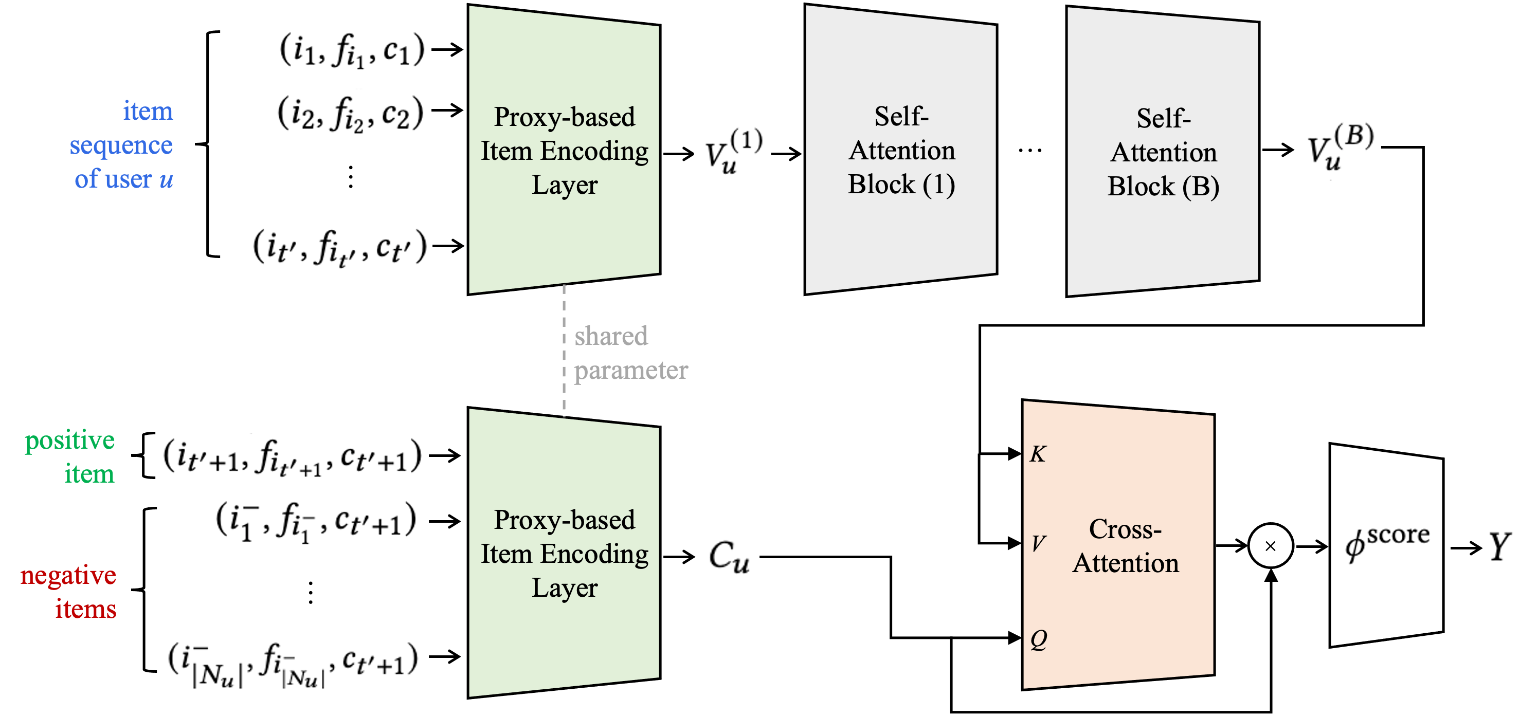
Figure 2. Overall model architecture.

Table 2. Dataset statistics after preprocessing.

Dataset	#user	#item	#interaction	Density	Unique Attributes	Duplicates	Memorization
Fashion	45,184	166,270	358,003	0.0048%	163,985	1.0	98.09%
Men	34,244	110,636	254,870	0.0067%	109,282	1.0	98.36%
Beauty	52,204	57,289	394,908	0.0132%	11,094	5.2	41.92%
Game	31,013	23,715	287,107	0.0390%	1,701	13.9	7.26%
ML-20M	138,287	20,720	9,995,410	0.3488%	1,342	20.3	4.92%

3.4. Complexity of Parameters

Since IE uses $|I|$ embeddings while $P$ only uses $n_{\text{proxy}}$ embeddings, the proxy-based item representation can reduce a significant number of parameters. For computational convenience, assume that all latent dimensions are equal to, or proportional to $d$: $d_{\text{IE}}=d$, $d_{\text{AC}}\propto d$, $d_{\text{A}}^{\prime}=d$, $d_{\varphi}\propto d$, and $d_{\text{proxy}}=d$. In a baseline model that uses IE, the number of parameters is $O(|I|d+M(d))$, where $M(d)$ is the number of parameters of the network other than the item embedding. For our model, the number of parameters is $O((K+d)n_{\text{proxy}}+M^{\prime}(d))$, where $M^{\prime}(d)$ denotes the number of parameters of the network other than the PIR layer. Note that in this case, the number of parameters does not increase proportionally to the number of items $|I|$. Even in the extreme case where $K=|I|$, parameters can be reduced whenever $n_{\text{proxy}}$ is just slightly smaller than $d$: let $n_{\text{proxy}}=\alpha d$, then we get $|I|d+M(d)>(|I|+d)n_{\text{proxy}}+M^{\prime}(d)\Leftrightarrow(|I|+d)^{-1}\left(|I|+(M(d)-M^{\prime}(d))/d\right)>\alpha$. Assuming that $M(d)\approx M^{\prime}(d)$, the model can shrink whenever $\alpha$ meets the condition (note that $d\ll|I|$ holds in general).

3.5. Training Objective

In sequential recommendation, it is common to create $|S_{u}^{\text{AC}}|-1$ tasks of Next Item Prediction (NIP) by using the aforementioned latent sequence vectors as user vectors, namely $V_{u,t}^{(B)}$ for each time step $1\leq t\leq|S_{u}^{\text{AC}}|-1$. However, in the case of cross-attention, the latent sequence vectors possess bidirectional information of the item sequence. Therefore, training cross-attention with NIP task incurs a discrepancy between the training phase and the inference phase since NIP assumes a causality constraint in the training phase. To this end, we adopt Last Item Prediction (LIP) task, which uses only the very last item of each user as a positive item. In every training epoch, each item sequence $S_{u}^{\text{AC}}$ is randomly cut (Wu et al., 2020) into a subsequence so that diverse input data can be trained for the same user. We also apply NT-Xent (Rendle et al., 2009; Sohn, 2016) on the cross-attention, so that the model can employ multiple negatives. We call this method Contrastive CA, where it can only be implemented in LIP task since it is not feasible to sample multiple negative items having the same context in NIP task due to the enormous memory cost. The final training objective is as follows: Assuming that for every epoch, each item sequence $S_{u}^{\text{AC}}$ of user $u$ is randomly cut, and $N_{u}$ is randomly sampled except for testing,

(19) $$\mathcal{L}=-|U|^{-1}\textstyle\sum_{u\in U}\log\left(e^{Y_{1}}/\textstyle\sum_{j=1}^{|I_{u}^{-}|+1}e^{Y_{j}}\right).$$

4. Experiment

To demonstrate the effectiveness of our proposed model, we have constructed experiments to answer the following research questions:

• RQ1 Does PIR layer show superior performance in a plug-and-play manner?

• RQ2 Does PIR layer enhance representation quality of infrequent items?

• RQ3 Does ProxyRCA have a parameter-efficient structure?

• RQ4 Do the proxy weights and proxy embeddings together compositionally compute item representations?

4.1. Experimental Settings

4.1.1. Datasets

To evaluate and analyze the proposed model, we use five widely used recommendation datasets from different domains, namely Fashion, Men, Game, and Beauty from Amazon Review datasets (McAuley et al., 2015), and MovieLens-20M (ML-20M). Fashion and Men use the image vectors extracted from the pre-trained ResNet50 model as their item attributes. Except for the price feature of Game, the attributes for Beauty and Game are discrete and categorical information, namely tags. In ML-20M, only the genre of each movie is used as item attributes, which represents the case where the content information are extremely limited. For contexts, timestamp data is decomposed into multi-dimensional date information, following the preprocessing steps in (Rashed et al., 2022). The overall statistics of the datasets are given in Table 2. In the preprocessing step, users with three or fewer interactions are excluded from the dataset to make a proper train-valid-test split.

Table 3. Performance comparison on all datasets. The best and the second best results are marked as bold and italic numbers respectively. The asterisk(*) denotes statistically significant (p ¡ 0.05) gain against the non-PIR counterpart, using the $t$-test.

Task	Model	Fashion		Men		Beauty		Game		ML-20M
		R@10	N@10	R@10	N@10	R@10	N@10	R@10	N@10	R@10	N@10
	Popular	0.407	0.262	0.415	0.269	0.451	0.261	0.519	0.314	0.815	0.530
BPR	BPR++	0.523	0.332	0.429	0.266	0.505	0.352	0.768	0.564	0.956	0.702
	$\,\hookrightarrow$ with PIR	0.620*	0.406*	0.554*	0.358*	0.511	0.353	0.770	0.582*	0.957	0.761*
LIP	MixDim++	0.623	0.407	0.570	0.365	0.587	0.398	0.766	0.556	0.961	0.781
	SASRec++	0.630	0.416	0.587	0.379	0.601	0.415	0.753	0.539	0.949	0.761
	$\,\hookrightarrow$ with PIR	0.635	0.426*	0.580	0.381	0.599	0.422	0.779*	0.572*	0.944	0.773*
	CARCA	0.648	0.427	0.614	0.398	0.608	0.423	0.762	0.560	0.961	0.788
	$\,\hookrightarrow$ with PIR (ProxyRCA)	0.661*	0.446*	0.617	0.408	0.626*	0.449*	0.809*	0.611*	0.962	0.792*

4.1.2. Evaluation Protocol

Overall, we follow the conventional evaluation protocol from the sequential recommendation studies (Rashed et al., 2022; He and McAuley, 2016; Kang and McAuley, 2018). We use the leave-one-out evaluation where the last item of each user is the test item, and the previous one to the last item is the valid item. A total of 100 negative items are randomly sampled among items that have not been interacted with the user. The performance is measured with Hit-Ratio (HR) and Normalized Discounted Cumulative Gain (NDCG), averaged over all users. We run 5 times each with different random seeds and report the average performance.

4.1.3. Comparison Models

For the fair comparison, we implemented the baseline models to have a similar structure and the same training objective (LIP task) to our setting. Full explanation and experimental results on NIP task baselines, namely BERT4Rec (Sun et al., 2019), SASRec (Kang and McAuley, 2018), SSE-PT (Wu et al., 2020), and S³Rec (Zhou et al., 2020) are in the appendix.

1. Popular: A non-personalized recommendation where the preference score is based on the item’s global popularity. It serves as a sanity check for the performance lower bound.

2. SASRec++ (Rashed et al., 2022): An extension of SASRec (Kang and McAuley, 2018) that utilizes item attributes and context.

3. CARCA (Rashed et al., 2022): A state-of-the-art ACSR model that uses cross-attention as an item scoring layer.

4. BPR++ (ours): An extension of the non-sequential model BPR (Rendle et al., 2009) that utilizes item attributes and context.

5. MixDim++ (ours): An extension of CARCA with parameter-efficient mixed-dimension embedding (Naumov et al., 2021) for encoding infrequent items. Note that this is an important baseline, which represents models that handle infrequent items (either long-tail or cold-start).

6. ProxyRCA (ours): This is our main proposed model that employs proxy-based item representation as the item encoding layer on top of CARCA, named after Proxy-based item representation Recommendation model with Cross-Attention.

4.1.4. Implementation Details

To match the similar scale of parameters, we fixed the latent dimension $d$ to 256, and $n_{\text{proxy}}$ was set to 128. We initialized $b_{i_{t}}^{\text{freq}}$ to be a zero vector in order to prevent the unintended influence on the computation of proxy weights in the early stages of the training. Detailed hyper-parameter tuning procedures are described in the appendix. The PyTorch-based implementation is shared as an open-source repository .

4.2. Overall Performance Comparison (RQ1)

Table 3 shows the overall performance comparison. We replaced the item encoding layer of three representative baselines, namely BPR++, SASRec++ and CARCA, and achieved performance improvement on almost all cases, as well as, all datasets in terms of NDCG. The final model, ProxyRCA reaches the state-of-the-art performance, improving up to 17% when compared to the previously reported results. The improvement on BPR model demonstrates that our PIR layer is not bound to sequential models. Interesting point is that Fashion and Men were previously known to be sensitive to sequential information, but with PIR, BPR++ reaches comparable performance to sequential models. Note that in any case, since we are using $n_{\text{proxy}}=0.5d$, only a minimum of 10% and a maximum of 50% of training parameters are used when compared to non-PIR counterparts. Moreover, our choice of the training objective, the LIP task, is generally superior to NIP task if tuned properly, which is shown in the appendix.

To further analyze the above results, we counted the unique number of attributes and the number of duplicate items for each attribute, and implemented a 2-layered neural network that takes item attributes as input to perform a memorization task of classifying items based on their attributes. The result is summarized in Table 2. In Fashion and Men, the item attributes distinguish the item accurately. In Game and ML-20M however, more than ten items share exactly the same attributes on average, and thus it is impractical to distinguish items by their attributes alone. Even with the datasets where attribute information is extremely weak, our ProxyRCA model can still outperform the baselines. We claim that the performance gain is due to the content-oriented shared embedding effect, similar to SSE (Wu et al., 2019), explaining why the model outperforms even with limited attribute information.

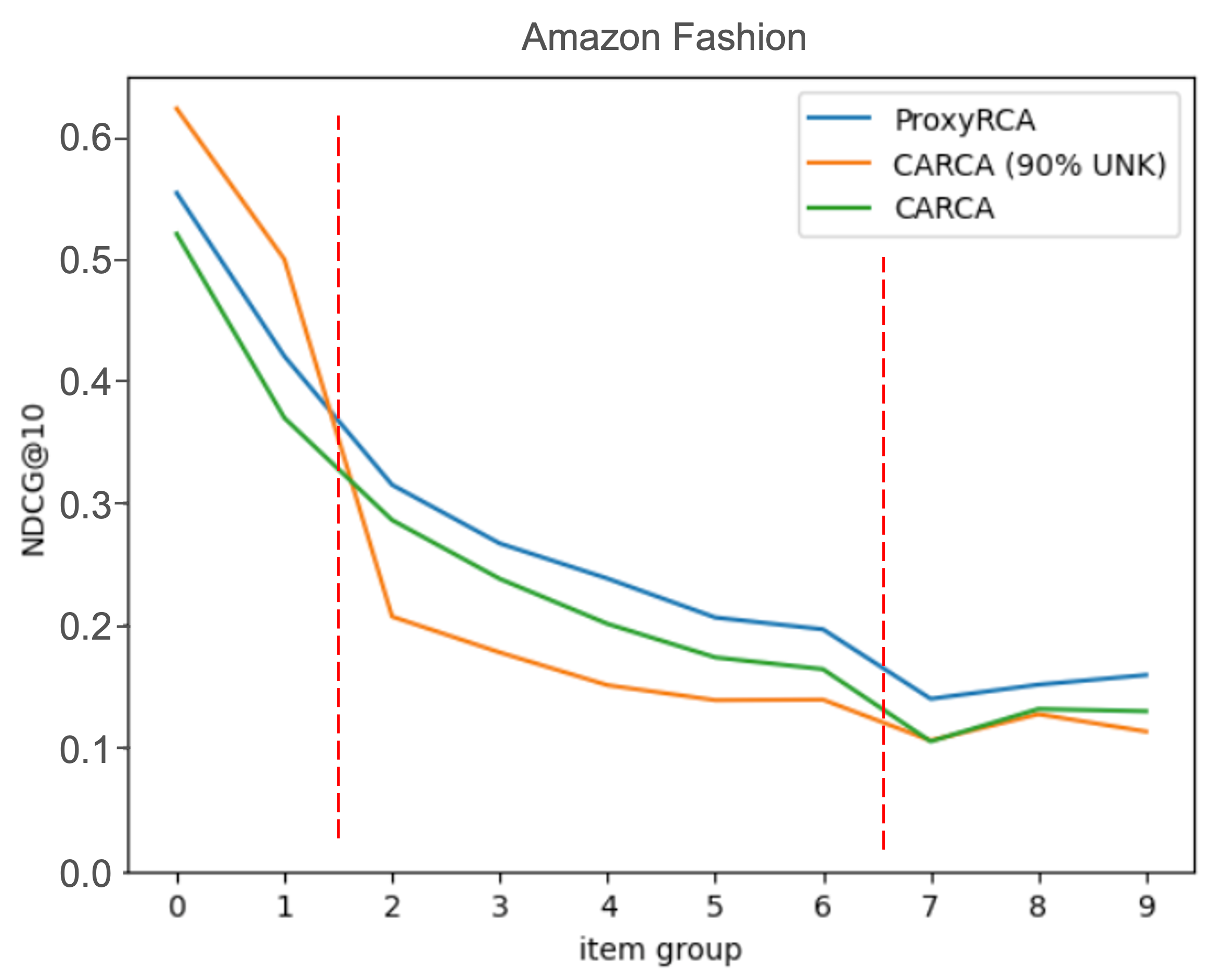
Figure 3. Performance comparison over frequency group.

4.3. Performance on Infrequent Items (RQ2)

As mentioned in Table 1, the baseline model showed a performance increase when infrequent item embeddings are replaced into the shared unknown token in sacrifice of the recommendation diversity. This phenomenon is not observed in models with PIR, which indirectly proves that the representation quality of the infrequent items is improved.

For further investigation, we divide items into 10 groups, sorted by frequency, so that the sum of item occurrence in each group is equal (i.e., the frequent group will have much fewer items compared to the infrequent group). We measure the mean performance of each group, average over each item on the test set, since an item can be a test item multiple times. The result is shown in Figure 3. For item groups 0 to 1, the baseline model with 90% of removal surmounts others but gives up the recommendation for majority of relatively infrequent item groups, which is an intuitive result. On the other hand, looking at item groups 7 to 9, CARCA does not show a big difference compared to the case of removing infrequent items, but ProxyRCA shows performance improvement in these groups as well, which also shows that the representation quality is improved.

4.4. Parameter Efficiency (RQ3)

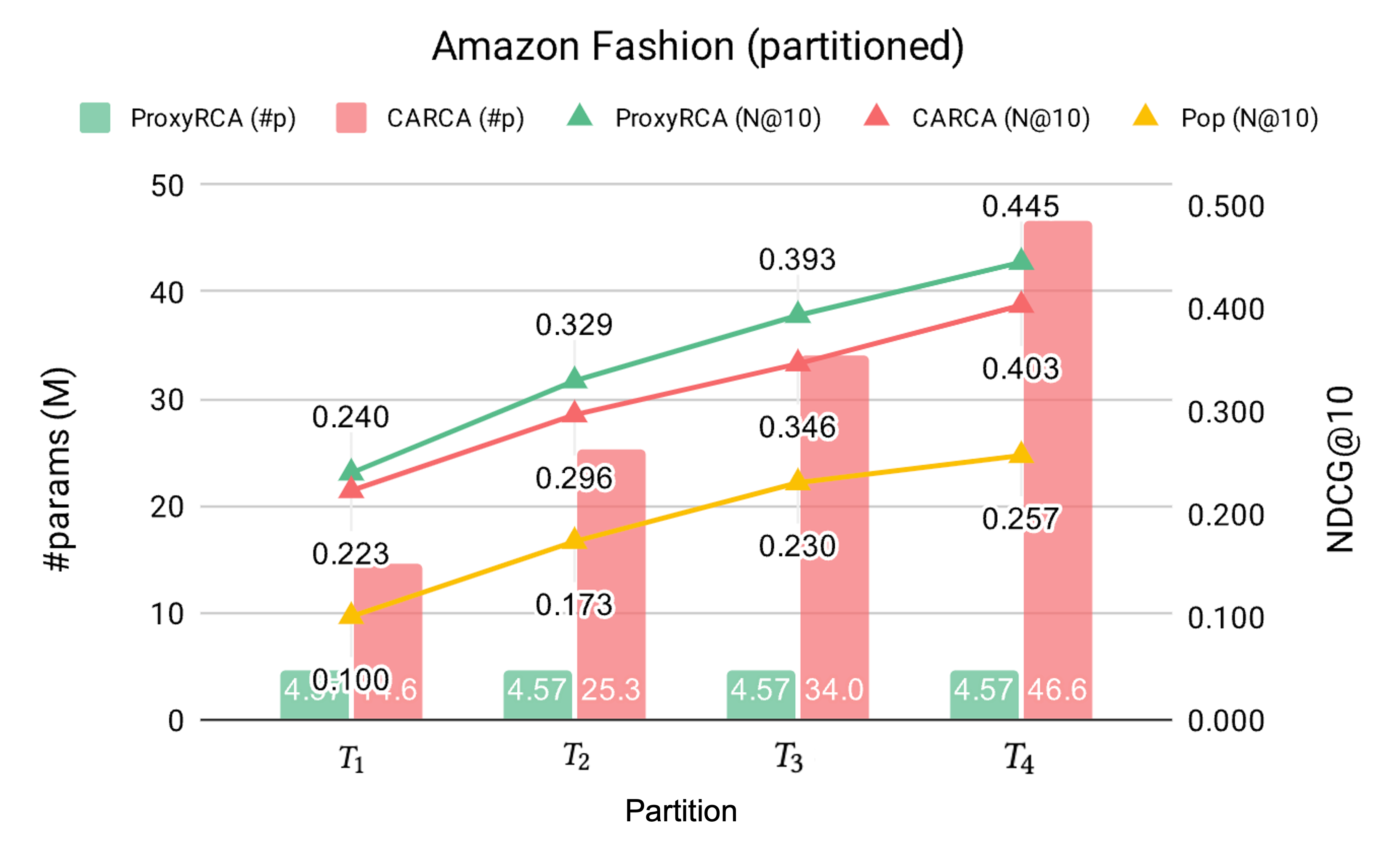
Figure 4. Parameter and performance comparison on the partitioned Fashion, simulating the growth of data.

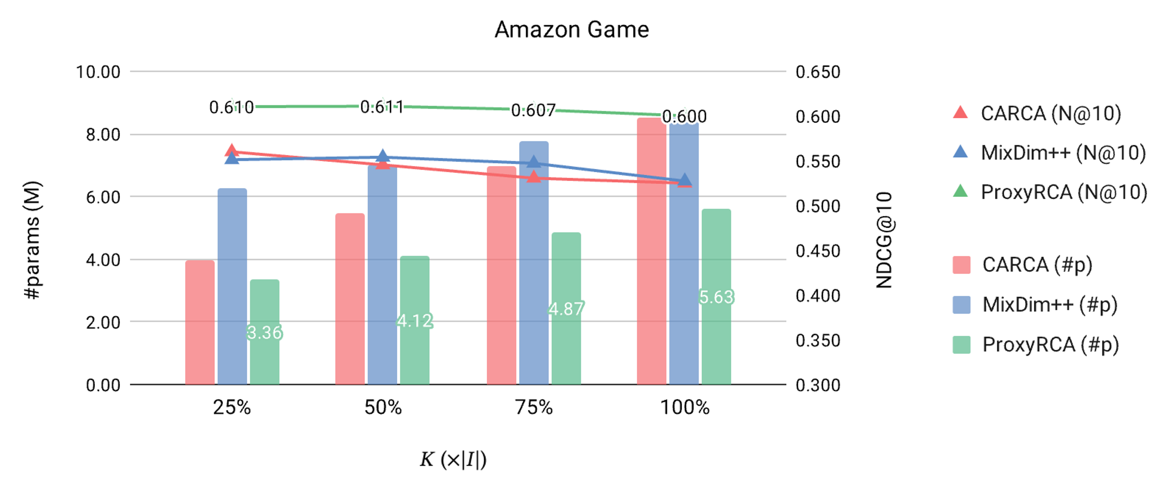
Figure 5. Parameter and performance comparison on Game over different $K$ value.

To demonstrate the parameter efficiency of ProxyRCA, we created four new datasets, namely Fashion $T_{r}$ ($r=1,2,3,4$) by truncating Fashion so that the number of items for each partition is equal to $r/4\times|I|$. These datasets simulate the real-world recommendation scenario where new items are added to the system. As shown in Figure 4, the baseline model continuously expands the look-up table to match the increasing number of items as $r$ increases. However, ProxyRCA succeeds in maintaining a superior performance with a fixed number of parameters.

To analyze the effect of the number of frequent items, we compare CARCA, MixDim++, and ProxyRCA in Game. For a fair comparison, CARCA treats items beyond top $K$ frequent items as unknown items, assigning the shared unknown embedding. For MixDim++, $K$ corresponds to the ratio of items using full latent dimension, while smaller dimension is set to $n_{\text{proxy}}$. The experiment result is in Figure 5. We can see that even with similar settings, ProxyRCA uses less parameters and slow parameter growth rate, with superior recommendation performance.

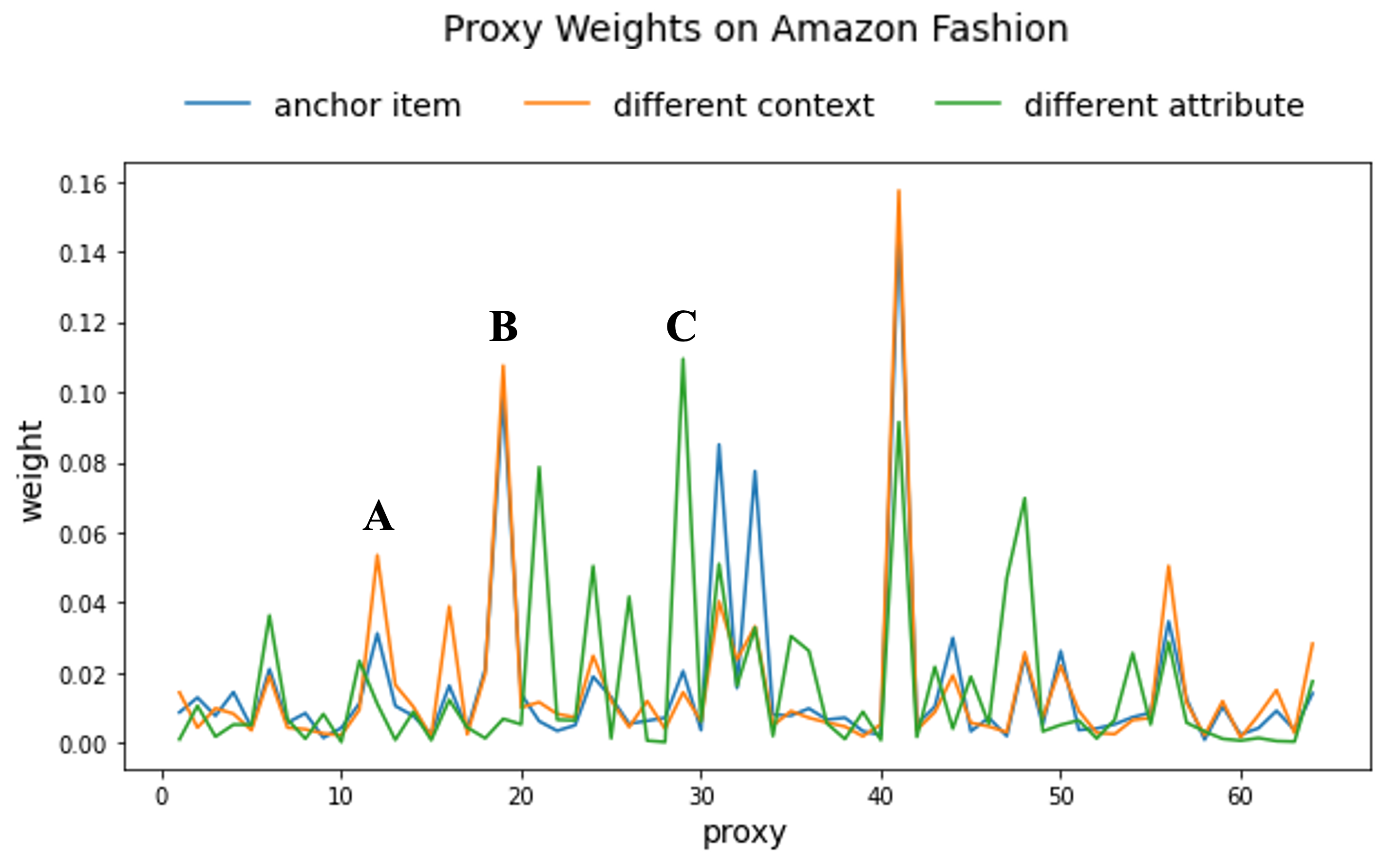
Figure 6. Visualization of proxy weights that reflect attribute and context modification.

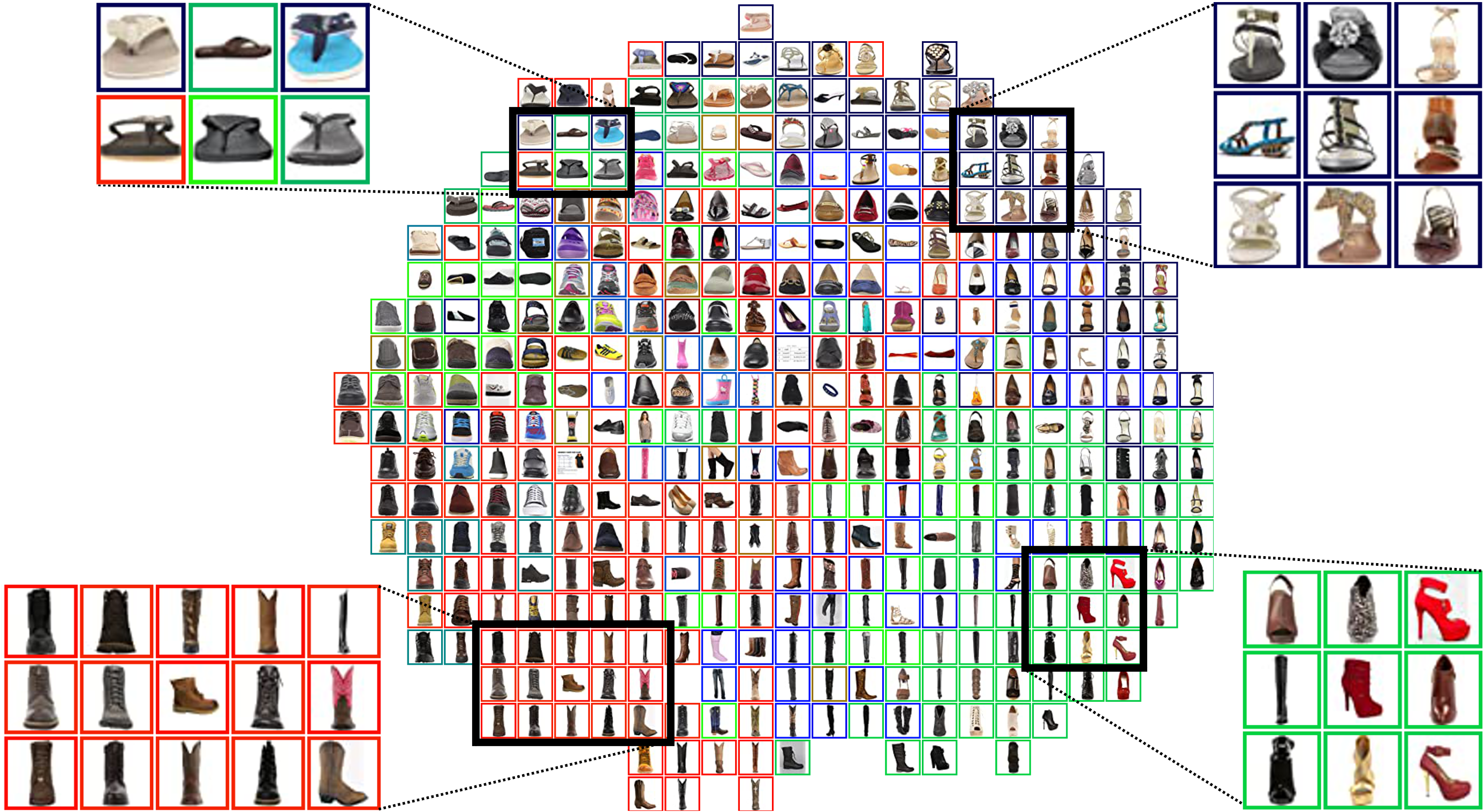
Figure 7. PCA visualization of item vectors on Fashion, using shoes category. The border colors denote the heaviest-weighted proxy.

4.5. Proxy Analysis (RQ4)

Since the proxy weights are mainly computed using item attribute and context, the weight values should be different when the attribute and context are changed without the frequent item bias. In Fashion, we first randomly choose an anchor item and visualize the computed proxy weights, as in Figure 6. To see the impact of context in proxy weights, we change context to an another value and visualize the weights. Similarly, to see the impact of attributes in proxy weights, we sample another item with different attributes but same context, and visualize the weights. As shown in the figure, due to the nature of Fashion that uses item images as attributes, the attributes are strongly reflected in the proxy weights. Therefore, we can see that most weights are similar when only contexts differ (points B and C in the figure). Even so, different context still assign different proxy weights (point A as demonstrated in the figure). This visualization indicates that each proxy has its role to represent items compositionally.

To show that the proxy-based item representation can also provide a clustering effect on infrequent items, we visualize the item vectors with $K=0$ using PCA, as in Figure 7. We use items of the shoes category among others (e.g., dress, outer) in Fashion to see if the model successfully captures the subcategory information without any labels, which is a rather challenging task when compared to supercategory clustering. The figure shows that the items of similar subcategories (e.g., flip-flops on top-left, sandals on top-right, boots on bottom-left, and pumps on bottom-right in the figure) are naturally clustered, even without any explicit labels.

5. Conclusion

In this paper, we highlighted the issues with the full-item embedding table from the perspective of infrequent item training through experimental demonstration. To overcome the issues, we proposed a proxy-based item representation model that can replace the existing item encoding layer in a plug-and-play fashion, by computing the item representation as a weighted sum of learnable proxy embeddings. To prove the effectiveness of our model, experiments were conducted using recommendation benchmark datasets and achieved state-of-the-art performance.

Appendix A Hyper-parameter Tuning

As a regularization, the weight decay is tuned among {0.0, 0.1, 0.2, 0.3} in AdamW (Loshchilov and Hutter, 2019) optimizer with learning rate of 0.0001, and the random item replace technique from (Wu et al., 2019) is used with the probability tuned among {0.0, 0.01, 0.02}. The maximum length of input sequence mostly depends on the dataset; however, the performance gain converges when it reaches a certain value, so we used similar values reported in (Rashed et al., 2022). The other hyper-parameters are tuned as follows: dropout probability in {0.0, 0.05, 0.1, 0.15, 0.2}, normalization layers as either LayerNorm (Ba et al., 2016) or $L_{2}$-norm, the number of self-attention blocks $B$ in {1, 2, 3, 4}, the number of attention heads $H$ in {1, 2, 4, 8}, random sequence cut probability in {0.0, 0.5, 1.0}, temperature $\tau$ of NT-Xent in {0.01, 0.1, 1.0}, and the number of frequent items $K$ in {0.0, 0.1, 0.25, 0.5, 0.75, 1.0} times the number of total items. Note that most hyper-parameters are not sensitive when they reside on a certain value range.

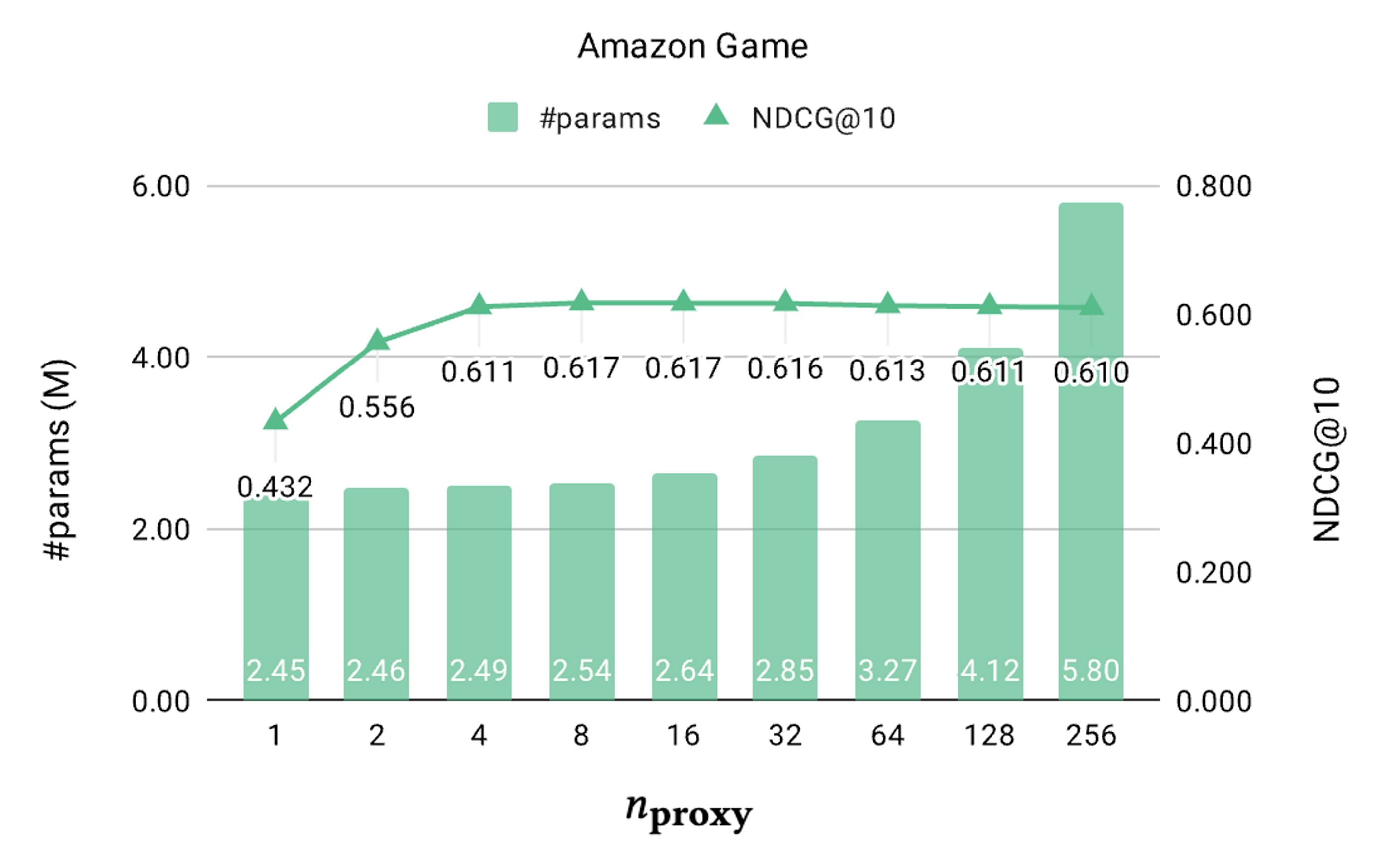
(a) Impact of $n_{\text{proxy}}$.

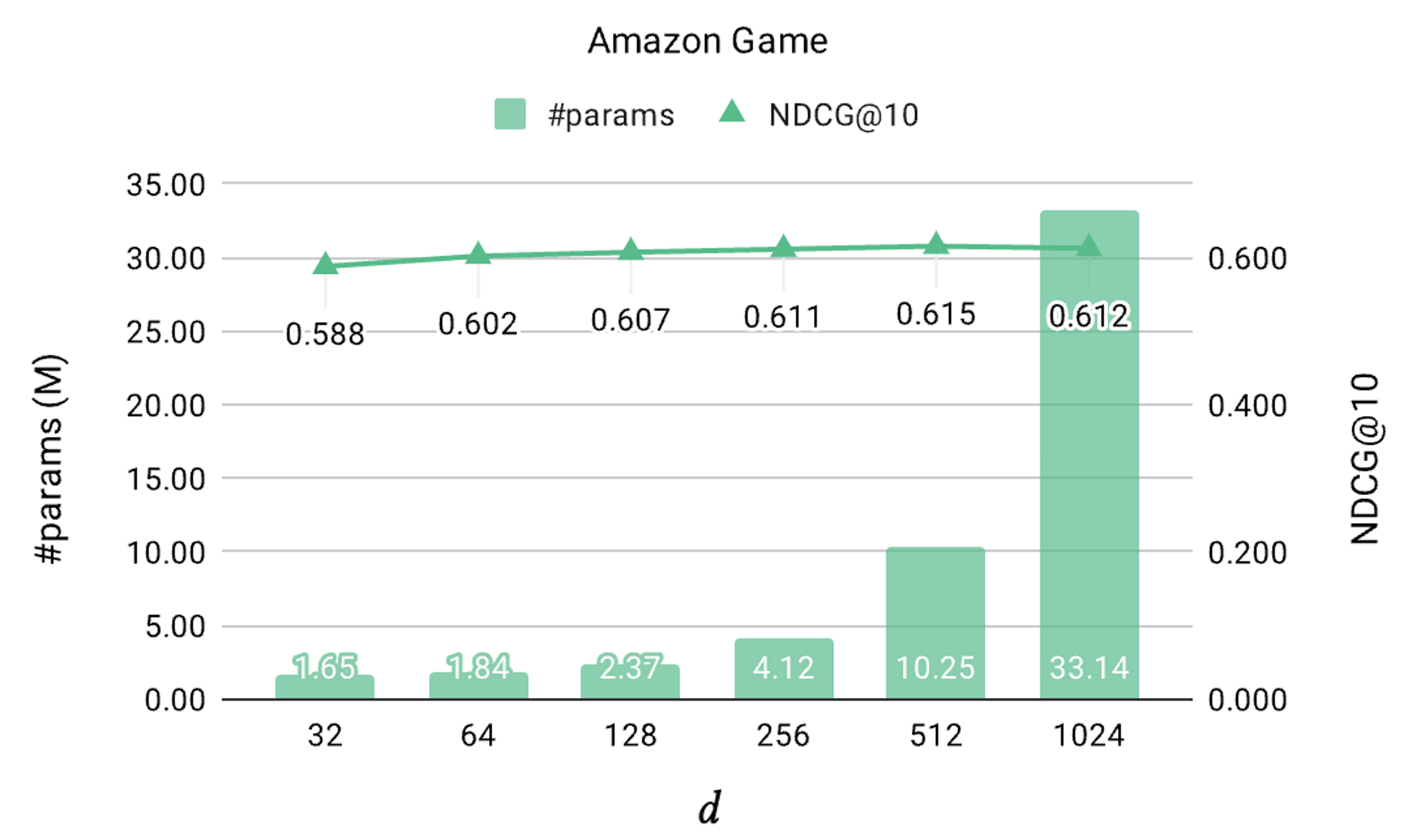
(b) Impact of $d$.

Figure 8. Impact of hyper-parameters on Game.

Appendix B Ablation Study

The main hyper-parameters of PIR are $n_{\text{proxy}}$ and a latent dimension $d$, where these two primarily determines the number of parameters. As shown in Figure 8(a), the model produces a similar performance once it reaches a certain number of proxies. Similarly, for the latent dimension, as demonstrated in Figure 8(b), it shows that the model is surprisingly robust to the dimension. This suggests that besides increasing the model parameters in the recommendation model, there is still room for further exploration of the model structure to improve the performance (Ardalani et al., 2022).

Appendix C Properties of Proxy-based Item Representation

Here, we prove the representation propositions proposed in the main section. Since the model network is complex, we indirectly claim that the concept of content locality and bias priority are sound.

Proposition C.1.

The proxy-based item representation without bias term has content locality.

Proof.

Let $f^{(1)},f^{(2)}\in\mathbb{R}^{n}$ be the content vectors of two items, right before the proxy weight computation. For simplicity, we assume that $\sum_{i=1}^{d}e^{f^{(1)}_{i}}=\sum_{i=1}^{d}e^{f^{(2)}_{i}}=Z$ and $f^{(1)}_{i}=f^{(2)}_{i}$ for $i=3,4,...,d$, and $f^{(1)}_{1}=f^{(1)}_{2}=g$. Without loss of generality, $f^{(2)}_{1}=f^{(1)}_{1}+\epsilon$ and $f^{(2)}_{2}=f^{(1)}_{2}-\delta$ hold for some $\epsilon,\delta>0$. Using the assumption, we can derive the $\delta$ as follow:

$$\,\,\,\,\sum_{i=1}^{d}e^{f^{(1)}_{i}}=\sum_{i=1}^{d}e^{f^{(2)}_{i}}$$

$$\Leftrightarrow \,\,\,\,e^{f^{(1)}_{1}}+e^{f^{(1)}_{2}}=e^{f^{(1)}_{1}+\epsilon}+e^{f^{(1)}_{2}-\delta}$$

$$\Leftrightarrow \,\,\,\,2e^{g}=e^{g+\epsilon}+e^{g-\delta}$$

$$\Leftrightarrow \,\,\,\,\delta=-\log(2-e^{\epsilon}),$$

with conditions of $\epsilon<\log(2-e^{-g})$. Now let $P\in\mathbb{R}^{n\times d}$ be proxy embeddings, then since the proxy weight is determined by the softmax of the content vectors, the item representation becomes $v=\text{softmax}(f)P$. Then the difference between two item representations is bounded above by using $\epsilon$:

$$\,\,\,\,\left\|v^{(1)}-v^{(2)}\right\|$$

$$= \,\,\,\,\left\|\text{softmax}(f^{(2)})P-\text{softmax}(f^{(2)})P\right\|$$

$$\leq \,\,\,\,\left\|P\right\|\left\|\text{softmax}(f^{(2)})-\text{softmax}(f^{(2)})\right\|$$ (matrix norm)

$$= \,\,\,\,\left\|P\right\|Z^{-1}e^{g}\left((1-e^{\epsilon})^{2}+(1-e^{-\delta})^{2}\right)^{\frac{1}{2}}$$

$$= \,\,\,\,\sqrt{2}\left\|P\right\|Z^{-1}e^{g}\left(e^{2\epsilon}-2e^{\epsilon}+1\right)^{\frac{1}{2}}.$$

Note that with Taylor expansion up to the second order, we can approximate $\left(e^{2\epsilon}-2e^{\epsilon}+1\right)^{\frac{1}{2}}\approx\epsilon$. ∎

Proposition C.2.

The proxy-based item representation with bias term has bias priority.

Proof.

Even with the same content vector, the bias term can control the proxy weight if necessary. If two bias terms are $b^{(1)}=[\infty,0,0,...,0]$ and $b^{(1)}=[0,\infty,0,...,0]$, then the weights are $w^{(1)}=\text{softmax}(f^{(1)}+b^{(1)})=[1,0,0,...,0]$ and $w^{(2)}=\text{softmax}(f^{(2)}+b^{(2)})=[0,1,0,...,0]$. Then, the final item representation is given as $w^{(1)}P=P_{1}$ and $w^{(2)}P=P_{2}$ respectively, which can denote completely different clusters. ∎

Table 4. Performance comparison on Amazon datasets, including baseline models with NIP task. The best and the second best results are marked as bold and italic numbers respectively. The asterisk(*) denotes statistically significant (p ¡ 0.05) gain against the non-PIR counterpart, using the $t$-test.

Task	Model	Fashion		Men		Beauty		Game
		R@10	N@10	R@10	N@10	R@10	N@10	R@10	N@10
	Popular	0.407	0.262	0.415	0.269	0.451	0.261	0.519	0.314
NIP	BERT4Rec	0.328	0.209	0.315	0.193	0.478	0.318	0.705	0.509
	SASRec	0.381	0.245	0.397	0.259	0.485	0.322	0.742	0.541
	SSE-PT	0.381	0.246	0.397	0.258	0.502	0.337	0.775	0.566
	S3Rec	0.367	0.239	0.365	0.238	0.538	0.371	0.765	0.549
	SASRec++	0.546	0.344	0.500	0.315	0.545	0.351	0.752	0.533
	CARCA	0.591	0.381	0.550	0.349	0.579	0.396	0.782	0.573
BPR	BPR++	0.523	0.332	0.429	0.266	0.505	0.352	0.768	0.564
	$\,\hookrightarrow$ with PIR	0.620*	0.406*	0.554*	0.358*	0.511	0.353	0.770	0.582*
LIP	MixDim++	0.623	0.407	0.570	0.365	0.587	0.398	0.766	0.556
	SASRec++	0.630	0.416	0.587	0.379	0.601	0.415	0.753	0.539
	$\,\hookrightarrow$ with PIR	0.635	0.426*	0.580	0.381	0.599	0.422	0.779*	0.572*
	CARCA	0.648	0.427	0.614	0.398	0.608	0.423	0.762	0.560
	$\,\hookrightarrow$ with PIR (ProxyRCA)	0.661*	0.446*	0.617	0.408	0.626*	0.449*	0.809*	0.611*
Improvement over previous state-of-the-art		11.9%	17.0%	12.2%	16.9%	8.1%	13.4%	3.5%	6.6%

Appendix D Additional Performance Comparison

D.1. Comparison Models

Here we explain the all baseline models, including models with NIP task.

1. Popular: A non-personalized recommendation where the preference score is based on the item’s global popularity. It serves as a sanity check for the performance lower bound.

2. BERT4Rec (Sun et al., 2019): A sequential recommendation model using masked language model task from BERT with a bidirectional Transformer encoder.

3. SASRec (Kang and McAuley, 2018): A model that performs autoregressive sequential recommendation based on a unidirectional Transformer encoder.

4. SSE-PT (Wu et al., 2020): An extension of SASRec that strengthens personalization by applying the stochastic shared embedding technique on user embeddings.

5. S³Rec (Zhou et al., 2020): An improved version of SASRec that adds various self-supervised tasks to leverage item attribute information further.

6. SASRec++ (Rashed et al., 2022): An extension of SASRec (Kang and McAuley, 2018) that utilizes item attributes and context. We experimented two versions that uses NIP and LIP tasks respectively.

7. CARCA (Rashed et al., 2022): A state-of-the-art ACSR model that uses cross-attention as an item scoring layer. Similar to SASRec++, we also compared two versions of NIP and LIP.

8. BPR++ (ours): An extension of the non-sequential model BPR (Rendle et al., 2009) that utilizes item attributes and context, with LIP task which uses multiple negative samples.

9. MixDim++ (ours): An extension of CARCA with parameter-efficient mixed-dimension embedding (Naumov et al., 2021) for encoding infrequent items. Note that this is an important baseline, which represents models that handle infrequent items (either long-tail or cold-start).

10. ProxyRCA (ours): This is our main proposed model that employs proxy-based item representation as the item encoding layer on top of CARCA, named after Proxy-based item representation Recommendation model with Cross-Attention.

D.2. Overall Performance Comparison

Table 4 shows the overall performance comparison, including baseline models that use NIP task. The results show that LIP task alone can contribute to the performance improvement (by comparing NIP and LIP versions of CARCA), but when the task is fixed, PIR independently contributes to the performance.