Chiral Modes of Giant Superfluid Vortices

Abstract

We discuss rapidly rotating states of a superfluid. We concentrate on the Giant-Vortex (GV) state, which is a coherent rotating solution with a macroscopic hole at the center. We show that, for any trap, the fluctuations obey an approximately chiral dispersion relation, describing arbitrary shape deformations moving with the speed of the ambient superfluid. This dispersion relation is a consequence of a peculiar infinite symmetry group that emerges at large angular velocity and implies an infinite ground-state degeneracy. The degeneracy is lifted by small corrections which we determine both for smooth traps and the hard trap.

I Introduction

Many systems with $U(1)$ symmetry break the symmetry spontaneously at low temperatures and at finite density. In particular, this was observed in He₄ and in trapped alkali-metal gases, which are in a superfluid phase at low temperatures. See [1, 2, 3] for reviews and references, among many others. Static superfluids contained in a trap have excitations with a linear dispersion relation $\omega=c_{\text{s}}|\vec{k}|$, where $c_{\text{s}}$ is the sound speed.

New physics emerges when the trap rotates and superfluids are stirred [4]. In $(2+1)$d, as the frequency of the trap increases vortices appear [5] and form an Abrikosov lattice [6]. In such a lattice, superfluid excitations (Tkachenko modes [7, 8, 9, 10]) have the dispersion relation $\omega\sim\vec{k}^{2}$ (see [11, 12] for a modern approach).

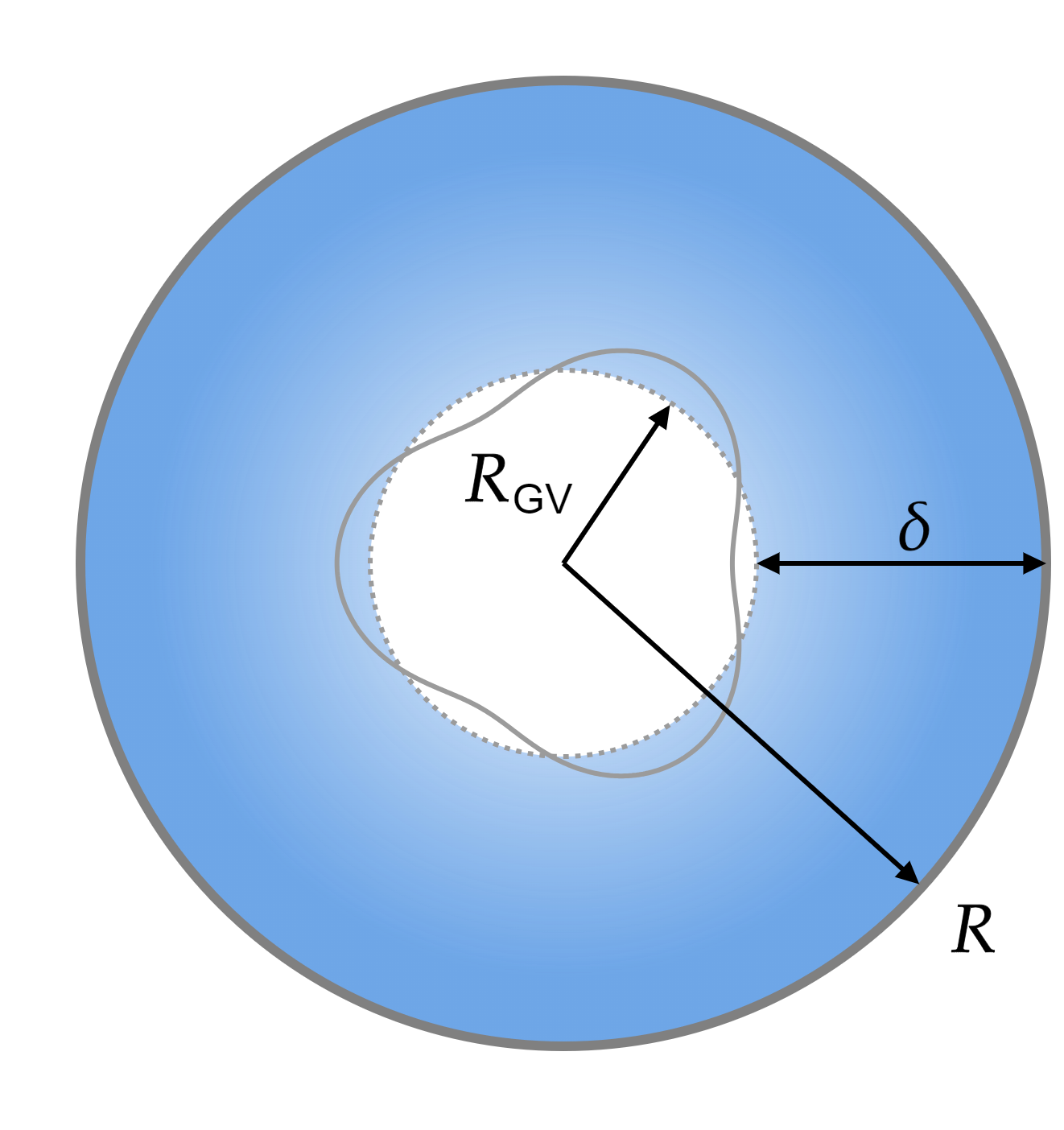
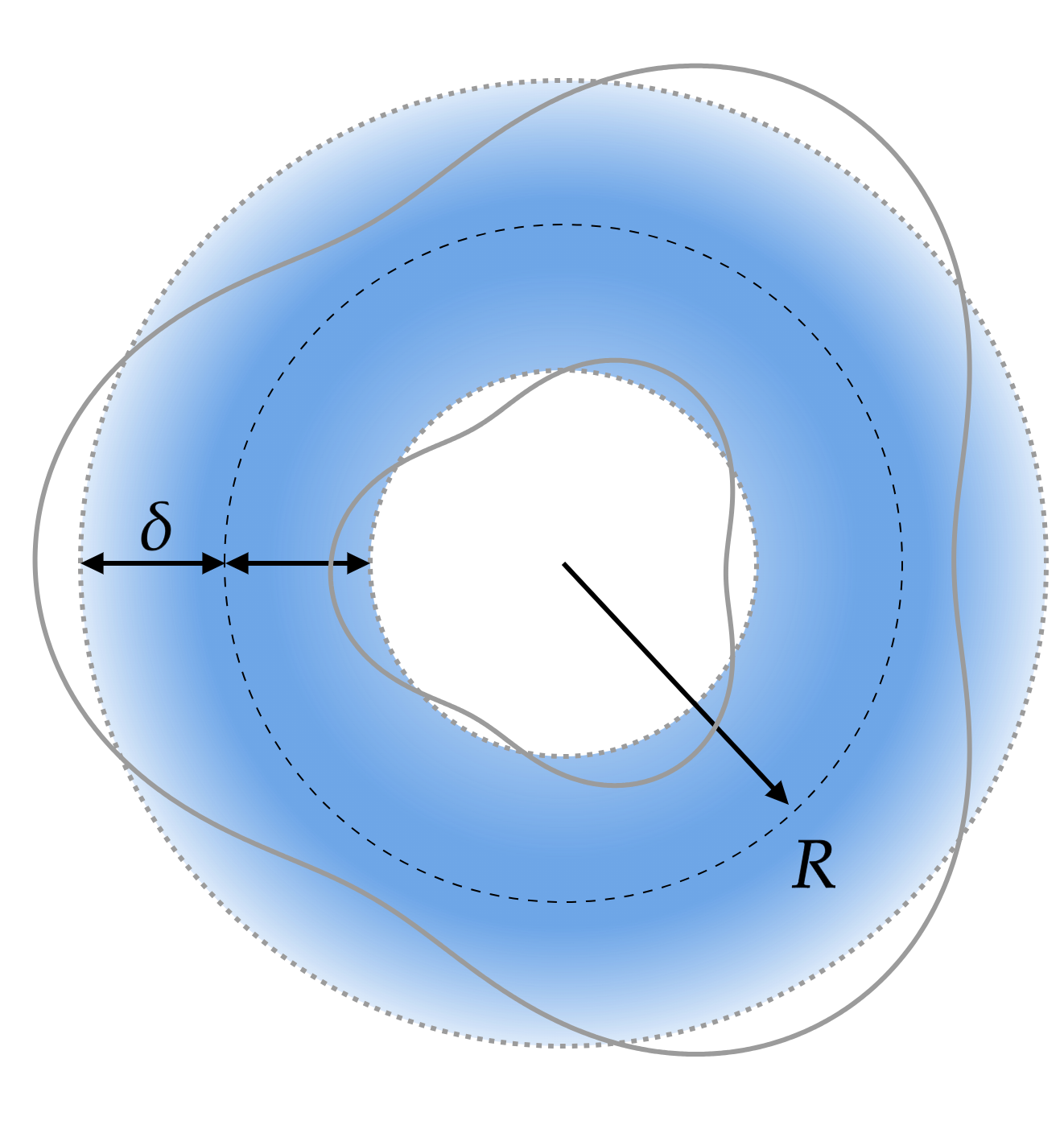
Figure 1: The GV of width $\delta$ and radius $R_{\text{GV}}$ in a hard cylindrical trap of radius $R$ (left) and in a smooth trap (right). Density fluctuations of the GV deform the shape of the edges and move together with the trap.

Above a certain trap frequency superfluids are expected to enter new phases. Here we concentrate on the Giant Vortex (GV) [13, 14, 15, 16]. This is a configuration with a large hole in the middle of the trap and no vorticity in the bulk of the superfluid, see Fig. 1. This configuration is expected to be stable at large angular velocity [14].

We study small density fluctuations of the (narrow) giant vortex, as in Fig. 1. We find that perturbations are chiral and approximately co-moving with the GV in the limit of large rotation speed $\Omega$:

$$\omega\simeq\Omega n~{},$$ (1)

where $n\in\mathbb{Z}$ is the angular momentum of the density perturbation. The fact that $n$ appears without absolute value leads to a peculiar infinite degeneracy of the ground state at fixed angular momentum. Indeed, Fock space states with $\sum n_{i}=0$ have the same quantum numbers and energy as the unperturbated GV.

As we make $\Omega$ larger at fixed particle number, the radius $R$ of the GV increases due to the centrifugal force, while the thickness $\delta$ becomes smaller. The lowest-lying excitations are approximately constant over the annulus radial direction. Therefore the effective theory of the fluctuations leading to (1) lives in 1+1 dimensions and describes the physics to leading order in $\delta/R$. The infinite degeneracy originates from peculiar symmetries of this $1+1$-dimensional effective field theory (EFT). At leading order in $\delta/R$ the EFT is invariant under the warped conformal group [17], as well as under a peculiar fractonic symmetry, reminiscent of [18, 19] (it also has many parallels with the chiral boson). The enormous ground state degeneracy is a consequence of these symmetries.

A useful way to think about (1) is that, in the rotating frame, the superfluid has a vanishing speed of sound. In reality, of course, the speed of sound is not vanishing but simply much smaller than $R\Omega$. This leads to $\delta/R$ suppressed corrections to the dispersion relation.

Indeed, in the limit $\delta\ll R$, the angular speed of sound in the rotating frame $c_{\text{s}}/R$ is much smaller than $\Omega$ and this leads to corrections to (1) of the form $\omega\simeq\Omega(n+\frac{c_{\text{s}}}{R\Omega}|n|)$, which lift the degeneracy of the ground state. In the main text, we compute explicitly the small corrections to (1). We find that these depend on certain details of the trap, in particular, its steepness. We do the calculation both for smooth and hard cylindrical traps.

Our central prediction is the existence of the chiral density fluctuations which move at the angular velocity of the trap. In the main text, we will see how small $\delta/R$ has to be in practice to see this effect. Intriguingly, recent experimental results suggest that the dispersion relation (1) might be a good approximation already at moderate rotation speed [20].

II Superfluid Effective Theory

We consider Galilean invariant superfluids in $2$ spatial dimensions. An important ingredient in the low-energy description of these systems is the Nambu-Goldstone boson $\phi\in\mathbb{S}^{1}$, which is the phase of the $U(1)$ order parameter. To the lowest order in derivatives, the effective action is written in terms of $\phi$ via the combination [21, 22] (we set $\hbar=1$ throughout)

$$X\equiv\partial_{t}\phi-V(x)-\frac{(\nabla\phi)^{2}}{2m}~{},$$ (2)

where $m$ is the mass of the microscopic constituents and $V(x)$ is the potential of the trap. $V(x)$ can be viewed as a background gauge field for particle number and hence we can write the effective action as a functional of $X$, valid for any trap. The static superfluid background is $\phi_{\text{cl}}=\mu t$, where $\mu$ is the chemical potential, and the expectation value of $X$ is $\langle X\rangle=\mu-V(x)$.

The effective action at low energies is a functional of $X$ with no additional derivatives,

$$S_{\text{EFT}}=\int dtd^{2}xP(X)~{}.$$ (3)

The effective theory for the fluctuations is obtained by expanding $P(X)$ around the classical background $\langle X\rangle$. $P(X)$ is identified as the thermodynamic pressure at the chemical potential $\langle X\rangle$. The particle number and current are given by $\rho=P^{\prime}(X)$ and $\vec{J}=-P^{\prime}(X)(\vec{\nabla}\phi)/m$.

In general, the functional $P(X)$ does not have to be analytic. The form of $P(X)$ depends on the UV details of the superfluid and it could be complicated even for weakly coupled microscopic models [23]. One well-studied UV completion is the $3+1$ dimensional Gross-Pitaevskii (GP) model confined in a region of height $h$,

$$\mathcal{L}_{\text{GP}}=\int_{0}^{h}dz\left[\Psi^{*}\left(i\partial_{t}+\frac{\nabla^{2}}{2m}-V\right)\Psi-\frac{\bar{g}}{4}|\Psi|^{4}\right].$$ (4)

The model (4) describes bosons with short-range repulsion in the s-wave ($\bar{g}=8\pi\ell_{\text{s}}/m>0$ where $\ell_{\text{s}}$ is the s-wave scattering length). The action (3) is derived from (4) setting $\Psi=e^{-i\phi}\sqrt{\rho/h}$, ignoring fluctuations in the $z$ direction, and integrating out $\rho$ in the Thomas-Fermi approximation $|\nabla^{2}\rho|\ll m\bar{g}\rho^{2}/h\,$. To leading order, this leads to the equation of state:

$$P(X)=\frac{m}{g}X^{2}\,.$$ (5)

where $g=m\,\bar{g}/h$. In the following, we will often use the equation of state (5) as a benchmark for our results.

The equation of motion for $\phi$ reads

$$m\partial_{t}P^{\prime}(X)-\nabla[P^{\prime}(X)(\nabla\phi)]=0~{}.$$ (6)

The equation of motion always admits classical solutions $\phi_{\text{cl}}=\mu t$. Since $\rho=P^{\prime}(x)$, the chemical potential $\mu$ controls the number of particles in the trap. Note that it is not physically meaningful to allow $P^{\prime}(X)$ to attain negative values - this restricts the domain of integration in (3) to the domain where $P^{\prime}(X)$ is positive. In general we expect $P^{\prime}(X)=0$ for $X=0$ [23]. Our equation of motion (6) has to be then supplemented by appropriate boundary conditions, as in [32, 33], to guarantee that particles do not flow through the boundary. Therefore, to the leading order in derivatives, we impose

$$\vec{J}\cdot\hat{n}=0$$ (7)

where $\hat{n}$ is transverse to the boundary of the superfluid.

Finally, expanding around the solution $\phi_{\text{cl}}=\mu t$ and neglecting the trapping potential, we find that phonons have dispersion relation $\omega=c_{\text{s}}|\vec{k}|$, where the speed of sound is given by

$$c_{\text{s}}^{2}=\frac{P^{\prime}(\mu)}{mP^{\prime\prime}(\mu)}\,.$$ (8)

III The giant vortex

When the trap is axisymmetric $V(x)=V(r)$, there is another set solutions to (6):

$$\phi_{\text{GV}}=\bar{\mu}t-L\theta\,,$$ (9)

where $L\in\mathbb{Z}$ is the vorticity and $\bar{\mu}$ should not be confused with the chemical potential. We assume for definiteness $L>0$. When $L\sim O(1)$, this solution describes a microscopic vortex and can be analyzed within the formalism of [34]. Here we are interested in the giant vortex limit $L\gg 1$, in which the vortex core is macroscopic. The properties of such solutions and fluctuations about these solutions are the main subject of this paper.

To warm up, let us consider the giant vortex in a hard trap which is a cylinder of radius $R$, and assume the equation of state (5). Then $X=\bar{\mu}-{L^{2}\over 2mr^{2}}$ which means that the density is non-negative in the domain $R\geq r\geq R_{\text{GV}}$ with $R_{\text{GV}}^{2}={L^{2}\over 2m\bar{\mu}}$. Therefore the superfluid occupies an annulus and is spinning with superfluid velocity ${L\over mr}$. We can relate $\bar{\mu}$ to the number of particles by integrating the density, leading to

$$N={\pi L^{2}\over g}\left({R^{2}\over R_{\text{GV}}^{2}}-2\log{R\over R_{\text{GV}}}-1\right)\,.$$ (10)

where we solved for $\bar{\mu}$ in terms of $R_{\text{GV}}$. Eq. (10) allows us to compute the radius of the giant vortex $R_{\text{GV}}$ in terms of the vorticity and the parameters of the trap and superfluid. If $R_{\text{GV}}$ is not too close to $R$, we would obtain approximately $R_{\text{GV}}\sim L\xi$ with the “healing length” $\xi^{-2}=g\rho$, and $\rho$ the density. (The healing length is the cutoff of (5).) We see that we need large vorticity $L\gg 1$ to create a macroscopic ($R_{\text{GV}}\gg\xi$) hole. For $R_{\text{GV}}=R-\delta$ with $\delta\ll R$, a narrow GV, we find:

$$N\simeq\frac{2\pi\delta^{2}L^{2}}{gR^{2}}\,\Rightarrow\,\delta\sim\frac{\Omega^{2}}{m^{2}\xi^{2}R}$$ (11)

where $\Omega=L/(mR^{2})$ is the angular velocity at the outer edge and the healing length is measured near $r=R$.

We remark that in this work we do not study in which regime the solution (9) is stable when working at fixed particle number and angular momentum. This question was studied in several previous works [39, 14, 15]. It is generally believed that, as the rotation speed of the trap is increased, the vortex lattice develops a macroscopic hole, and the superfluid eventually settles in a giant vortex state.   We plan to reexamine this process in a future work [41].

IV Fluctuations in the hard trap for the Gross-Pitaevskii model

We now study the fluctuations of the giant vortex in a hard trap with the equation of state (5). An axially symmetric trap breaks explicitly boosts and translations. Additionally, the solution (9) breaks spontaneously the $U(1)$ particle number $N$, time translations $H$ and rotations $J$ down to the two linear combinations $H-\bar{\mu}N$ and $J-LN$. The existence of these two unbroken generators allows us to organize fluctuations into modes with well-defined frequencies and angular momentum. In contrast, the vortex lattice does not admit an unbroken rotation generator.

We denote the fluctuation field $\varphi\in\mathbb{S}^{1}$ and write $\phi=\phi_{\text{GV}}+\varphi$. We will assume that $\varphi$ does not wind around the $\theta$-coordinate to avoid double counting of the modes. The fluctuation Lagrangian to quadratic order reads

$$\mathcal{L}_{\text{flu}}= \frac{m}{g}\left(\partial_{t}\varphi+\frac{L}{mr^{2}}\partial_{\theta}\varphi\right)^{2}$$ (12)

$$-\frac{L^{2}}{2mg}\left({1\over R_{\text{GV}}^{2}}-{1\over r^{2}}\right)(\nabla\varphi)^{2}\,.$$

We study the fluctuations with the ansatz $\varphi=e^{-i\omega t+in\theta}Y(r)$. The problem simplifies if we denote $R_{\text{GV}}/R=\sqrt{\lambda/(\lambda+1)}$ with $\lambda\in\mathbb{R}^{+}$, such that $\lambda\ll 1$ is the limit where the GV hole is small compared to the disk size while $\lambda\gg 1$ is the limit of a narrow GV. Furthermore, we introduce a new coordinate $z\in\mathbb{R}^{+}$ and let $r/R=\sqrt{(\lambda+e^{-z})/(\lambda+1)}$. The equation of motion in terms of $Y$ reduces to a Schrödinger problem

$$-\partial_{z}^{2}Y+\mathcal{V}(z)(Y/4)=0\,,$$ (13)

where

$$\mathcal{V}(z)=\left(\frac{n}{\lambda e^{z}+1}\right)^{2}-\frac{2\lambda}{e^{z}}\left(\frac{\omega mR^{2}}{L(\lambda+1)}-\frac{ne^{z}}{\lambda e^{z}+1}\right)^{2}\,,$$ (14)

and the boundary condition reads $\partial_{z}Y=0$ at $z=0$ as well as $z=+\infty$.

At the inner edge of the GV, $z\gg 1$, the potential is

$$\mathcal{V}(z)=-\frac{2}{\lambda}\left[\frac{\omega mR_{\text{GV}}^{2}}{L}-n\right]^{2}e^{-z}+O\left(e^{-2z}\right)\,.$$ (15)

The potential is always attractive (negative), unless $\frac{\omega mR_{\text{GV}}^{2}}{L}-n=0$. This is a striking feature: despite the fast swirling of the superfluid, one finds that some phonons are attracted to the inner edge of the GV.

We only discuss in detail the narrow limit $\lambda\rightarrow\infty$. Then we find the radial wave functions $Y=J_{0}\big{(}ke^{-z/2}\big{)}$ with wave number $k=\sqrt{2/\lambda}|\omega mR_{\text{GV}}^{2}/L-n|$. $k$ is quantized by virtue of the boundary conditions at the hard trap. We get that either $k=0$ or $k_{n^{\prime}}=j_{1,{n}^{\prime}}$, where $j_{a,b}$ is the $b$-th zero of the Bessel function $J_{a}$. The modes with a nontrivial radial profile $n^{\prime}>0$ lead to the dispersion relation

$$\omega_{n,{n}^{\prime}}=\Omega\left[n+\sqrt{\frac{R}{\delta}}\frac{j_{1,{n}^{\prime}}}{2}+O\left(\sqrt{\frac{\delta}{R}}\right)\right]\,,$$ (16)

Due to the nontrivial profile over the annulus width, eq. (16) yields a large gap $\omega-\Omega n\sim\Omega\sqrt{R/\delta}$ in the rotating frame.

The states $k=0$ are much more interesting. We find a mode with profile $Y=1+O(\delta^{2}/R^{2})$ and dispersion

$$\omega_{n,0}=\Omega\left[n+\sqrt{\frac{\delta}{2R}}|n|+O\left(\frac{\delta}{R}\right)\right]~{}.$$ (17)

Here we included the small correction $\sqrt{\frac{\delta}{2R}}|n|$ compared to (1). These states are the chiral modes since their gap $\omega-\Omega n$ in the rotating frame is much smaller than the angular velocity. To leading order in $\delta/R$, their shape is arbitrary and they are co-moving with the trap. See Fig. 2 for a summary of the spectrum in the hard trap.

V Fluctuations in the hard trap for arbitrary $P(X)$

We now generalize the discussion in the former section to an arbitrary equation of state $P(X)$. We focus directly on the experimentally relevant narrow limit. We linearize $\langle X\rangle$ around the edge $r=R$, at which it is peaked:

$$\langle X\rangle=\mu_{\text{eff}}(1+y)\left[1-\frac{3\delta}{R}y+O\left(\frac{\delta^{2}}{R^{2}}\right)\right]\,,$$ (18)

where $\delta=R-R_{\text{GV}}$ is the thickness of the annulus, $\mu_{\text{eff}}=\bar{\mu}-m\Omega^{2}R^{2}/2$, and $y=(r-R)/\delta\in[-1,0]$. We imposed that $\langle X\rangle$ vanishes in the inner edge $y=-1$.

The thickness $\delta$ and chemical potential $\mu_{\text{eff}}$ depend upon the angular velocity $\Omega=L/(mR^{2})$, $R$, and the number of particles. A crude measure for the speed of sound in the rotating frame, similarly to eq. (8), is $c_{\text{s,eff}}^{2}=P^{\prime}(\mu_{\text{eff}})/[mP^{\prime\prime}(\mu_{\text{eff}})]$, which is roughly the speed of sound in the rotating frame near the outer edge $r=R$. For a generic equation of state, we expect the scaling $c_{\text{s,eff}}^{2}\sim\mu_{\text{eff}}/m$. To obtain the relation we are after, we notice that eq. (18) implies $\mu_{\text{eff}}/\delta\simeq L^{2}/(mR^{3})=m\Omega^{2}R$, therefore

$$\Omega^{2}\simeq\frac{\mu_{\text{eff}}}{m\delta R}\sim\frac{c_{\text{s,eff}}^{2}}{\delta R}\,.$$ (19)

This relation together with the condition $\int d^{2}xP^{\prime}(\langle X\rangle)=N$ determines $\mu_{\text{eff}}$ and $\delta$ in terms $\Omega$ and $R$.

As explained above, we expect chiral modes whose energy in the rotating frame scales as $\omega-\Omega n\sim c_{s,eff}/R\sim\Omega\sqrt{\delta/R}$, where we used the scaling (19). This estimate agrees with the result (17) in the quadratic model. In practice, the exact expression depends upon the equation of state.

We analyze the spectrum of fluctuations in a series expansion for $\delta/R\ll 1$. This amounts to an expansion of the equations of motion analogously to what we did in (18). The details are in the supplemental material. For the modes with a nontrivial profile in the radial direction we find

$$\omega_{n,n^{\prime}}=\Omega\left[n+\sqrt{\frac{R}{\delta}}k_{n^{\prime}}+O\left(\sqrt{\frac{\delta}{R}}\right)\right]\,,$$ (20)

where $k_{n^{\prime}}$ is an $O(1)$ number which depends upon the equation of state. For the quadratic model (5) we found in eq. (16) $k_{n^{\prime}}=j_{1,n^{\prime}}/2$.

The $n^{\prime}=0$ chiral modes in eq. (20) again require a separate treatment and a computation of subleading corrections. We arrive at the final result

$$\omega_{n,0}=\Omega\left[n+\alpha_{P}\sqrt{\frac{\delta}{R}}|n|+O\left(\frac{\delta}{R}\right)\right]$$ (21)

where the coefficient is given by

$$\alpha_{P} =\sqrt{\frac{\int d^{2}x{P}^{\prime}\left(\langle X\rangle\right)}{\mu_{\text{eff}}\int d^{2}x{P}^{\prime\prime}\left(\langle X\rangle\right)}}>0\,.$$ (22)

where $\langle X\rangle$ is evaluated to its leading order in $\delta/R$. Physically, $\alpha_{P}$ is an averaged sound speed in units of $\sqrt{\mu_{\text{eff}}/m}$. The term proportional to $\alpha_{P}$ in eq. (21) lifts the pathological degeneracy of the ground state.

VI Fluctuations in Smooth Traps

We finally discuss the narrow GV in a smooth trap $V(r)$. The superfluid resides between the zeroes of the density $P^{\prime}(X)$. We assume that these coincide with the zeroes of $X=\bar{\mu}-V(r)-{L^{2}\over 2mr^{2}}$. We define $R$ to be the point at which $\langle X\rangle$ reaches its maximum, i.e. we have

$$0=\frac{L^{2}}{mR^{3}}-V^{\prime}(R)=m\Omega^{2}R-V^{\prime}(R)\,,$$ (23)

where in the last equality $\Omega=L/(mR^{2})$ denotes the angular velocity at the point $r=R$. We also assume that (23) admits a unique solution. This is for instance the case for the power law trap, among others.

In the narrow limit, it is convenient to expand $\langle X\rangle$ near its maximum similarly to eq. (18). Because of eq. (23) the expansion starts at quadratic order:

$$\langle X\rangle=\mu_{\text{eff}}\left[1-y^{2}+c_{3}\frac{\delta}{R}y^{3}+O\left(\frac{\delta^{2}}{R^{2}}\right)\right]\,,$$ (24)

where $\mu_{\text{eff}}=\bar{\mu}-\frac{1}{2}M\Omega^{2}R^{2}-V(R)$, $\mu_{\text{eff}}/\delta^{2}=\frac{1}{2}V^{\prime\prime}(R)+\frac{3}{2}M\Omega^{2}$, and we defined a new variable $y=(r-R)/\delta$. Therefore $R$ approximately coincides with the center of the annulus, and the superfluid density vanishes at $y\simeq\pm 1$. This approximation is accurate as long as the potential $V(r)$ is not too steep, e.g. for $V(r)\sim r^{q}$ we find $q\ll R/\delta$.

Let us consider the relation between $\mu_{\text{eff}}$, $\delta$ and $\Omega$ analogous to eq. (19). The fact that the expansion in eq. (24) starts at quadratic order implies an important difference with respect to the hard trap. For a sufficiently smooth trap, we expect the scaling $V^{(n)}\sim m\Omega^{2}R^{2-n}\sim L^{2}/(MR^{2+n})$. Therefore from the definition of $\delta$ below eq. (24) we infer that

$$\Omega^{2}\sim\frac{\mu_{\text{eff}}}{m\delta^{2}}\sim\frac{c^{2}_{\text{s,eff}}}{\delta^{2}}\,.$$ (25)

Note that this estimate differs by a factor $R/\delta$ compared to eq. (19). Therefore for a smooth trap, we expect chiral modes whose gap in the rotating frame scales as $c_{\text{s,eff}}/R\sim\Omega\delta/R$, which is a smaller gap than the result (21) $\sim\Omega\sqrt{\delta/R}$ for the hard trap.

The calculation of the spectrum proceeds analogously to the previous section. It turns out that in the narrow limit, the information about the trapping potential is contained in the following factor

$$\gamma_{V}\equiv\sqrt{\frac{\mu_{\text{eff}}}{2m}}\frac{1}{\delta\Omega}=O(1)\,.$$ (26)

$\gamma_{V}$ roughly characterizes the steepness of the trap around $r=R$. For example in a power-law trap, $V\sim r^{q}$ reads $\gamma_{V}=\sqrt{(q+2)/4}$. We obtain the following spectrum:

$$\omega_{n,n^{\prime}}=\Omega\left[n+\sqrt{2}\gamma_{V}k_{n^{\prime}}+O\left(\frac{\delta}{R}\right)\right]\,.$$ (27)

The $n^{\prime}=0$ solutions have $k_{0}=0$ and $Y=\text{const}.$: these are the chiral modes that we will discuss separately. Remarkably, we also find another set of solutions, $n^{\prime}=1$, for which we universally have $k_{1}=\sqrt{2}$. (These can be interpreted as approximate gapped Goldstone modes - see the supplementary material.) The solutions $n^{\prime}>1$ depend upon the equation of state and have $k_{n}^{\prime}>\sqrt{2}$, with frequencies $\sim c_{\text{s,eff}}/\delta$. As an example, in the model (5) we find $k_{n^{\prime}}=\sqrt{n^{\prime}(n^{\prime}+1)}$.

The calculation of the subleading correction to the frequency of the chiral modes again proceeds analogously. Interestingly, these are non-tachyonic only as long as $\gamma_{V}>1$, i.e. as long as the trap is steep enough. For instance, a power-law trap needs to be steeper than quadratic. Notice that the same is true for the vortex lattice. Physically, this is because we need the potential to balance the centrifugal force.

The result for the frequency of the chiral modes at subleading order reads

$$\omega_{n,0}=\Omega\left[n+\alpha_{P}\sqrt{2(\gamma_{V}^{2}-1)}|n|\frac{\delta}{R}+O\left(\frac{\delta^{2}}{R^{2}}\right)\right]\,,$$ (28)

where $\alpha_{P}$ is defined as in (22). See Fig. 2 for a qualitative summary of the spectrum of the GV both in the hard and in the smooth trap.

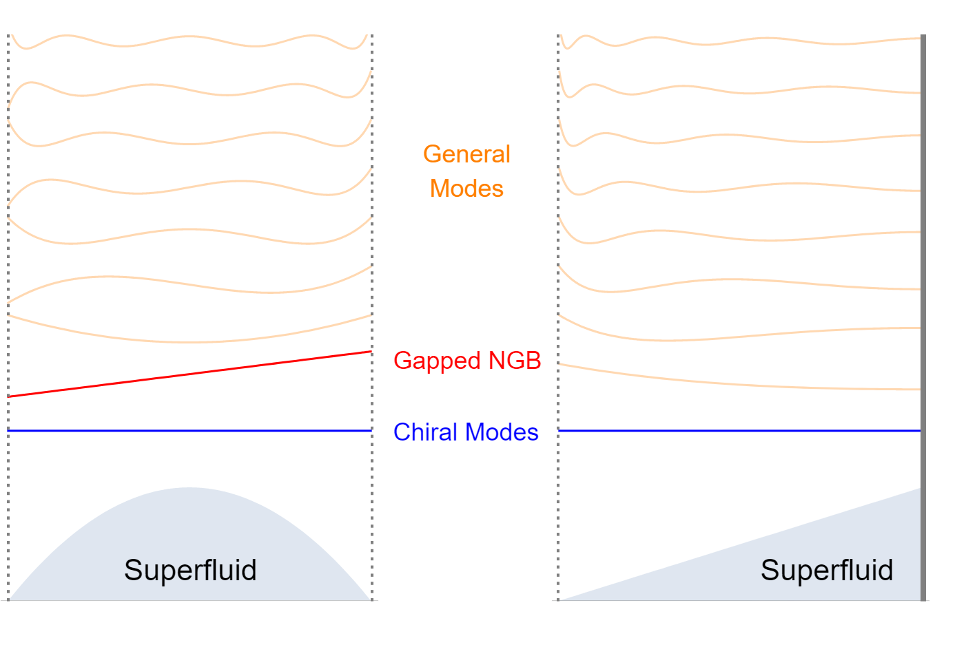
Figure 2: The superfluid density profile and density excitations in the smooth trap (left) and the hard trap (right).

VII EFT of the Narrow Giant Vortex

Here we discuss the EFT of the superfluid phase that leads to the peculiar infinite degeneracy of the ground state at fixed angular momentum. The leading order theory from which (1) follows is

$$S\sim\int dtd\theta\left(\partial_{t}\varphi+\Omega\partial_{\theta}\varphi\right)^{2}\sim\int dx^{+}dx^{-}(\partial_{+}\varphi)^{2}~{}.$$ (29)

where we switched to the coordinates $x^{\pm}=t\pm mR^{2}\theta/L$. This action has the chiral conformal symmetry $x^{-}\to f(x^{-})$ with $\varphi\to\varphi/\sqrt{f^{\prime}(x^{-})}$ as well as chiral translations $x^{+}\to x^{+}+g(x^{-})$. These furnish the so-called warped conformal group, see e.g. [17]. Additionally, the action (29) admits the fractonic shift symmetry $\varphi\rightarrow\varphi+f(x^{-})$. This last symmetry group implies the existence of infinitely many chiral solutions with zero energy and it is therefore responsible for the enormous ground state degeneracy. Corrections to (29) lift this degeneracy. From the perspective of the effective theory (29), corrections arise from the term $\sim\frac{c_{\text{s,eff}}^{2}}{R^{2}}\int dx^{+}dx^{-}(\partial_{\theta}\varphi)^{2}$ and lead to the required modification in the dispersion relation.

Further small corrections which we compute in the supplementary material for smooth traps remove the remaining degeneracy in excited states. The degeneracy among excited states is split due to a higher derivative term such as $\sim\int dx^{+}dx^{-}(\partial^{2}_{\theta}\varphi)^{2}$ as we illustrate in the supplementary material.

VIII Acknowledgments

We thank K. Jensen for useful discussions and A. Nicolis for useful discussions and collaboration on a related project. GC is supported by the Simons Foundation grant 994296 (Simons Collaboration on Confinement and QCD Strings). ZK and SZ are supported in part by the Simons Foundation grant 488657 (Simons Collaboration on the Non-Perturbative Bootstrap), the BSF grant no. 2018204 and NSF award number 2310283.

IX Supplemental Material

With a general equation of state, the Lagrangian density for the fluctuations is

$$\mathcal{L}_{\text{flu}}=\frac{{P}^{\prime\prime}(\langle X\rangle)}{2}\left(\partial_{t}\varphi+\frac{L}{mr^{2}}\partial_{\theta}\varphi\right)^{2}-\frac{{P}^{\prime}(\langle X\rangle)}{2m}(\nabla\varphi)^{2}\,.$$ (30)

Formally, to leading order in $\delta/R$, the equations of motion take the same form for both the smooth and the hard trap. To see this we express $\langle X\rangle=\langle X\rangle_{0}+O(\delta/R)$, where $\langle X\rangle_{0}$ is the leading term in eq.s (18) and (24). We expand the terms in eq. (30) as

$$\frac{L}{mr^{2}}\partial_{\theta}\varphi=\Omega\left[\partial_{\theta}\varphi-2y\partial_{\theta}\varphi\frac{\delta}{R}+O\left(\frac{\delta^{2}}{R^{2}}\right)\right]\,,$$ (31)

$$(\nabla\varphi)^{2}=\frac{1}{R^{2}}\left[\frac{R^{2}}{\delta^{2}}(\partial_{y}\varphi)^{2}+(\partial_{\theta}\varphi)^{2}+O\left(\frac{\delta}{R}\right)\right]\,$$ (32)

where $y$, $\delta$ and $R$ are defined below (18) for the hard trap, and below (24) for a smooth trap.

It is then straightforward to derive the equations of motion and solve them perturbatively in $\delta/R$. We adopt the ansatz $\varphi=e^{-i\omega t+in\theta}Y(r)$ and we find the following equation at leading order:

$$m\delta^{2}(\omega-\Omega n)^{2}{P}^{\prime\prime}(\langle X\rangle_{0})Y(y)+\partial_{y}\left[{P}^{\prime}(\langle X\rangle_{0})Y^{\prime}(y)\right]=0\,.$$ (33)

This is a second order ODE for $Y(y)$, subject to the boundary conditions (7), which explicitly read

$${P}^{\prime}(\langle X\rangle_{0})Y^{\prime}(y)=0\,.$$ (34)

at the boundary of the annulus.

IX.1 The Hard Trap

In a hard trap, we have $\langle X\rangle_{0}=\mu_{\text{eff}}(1+y)$ and $\mu_{\text{eff}}=m\Omega^{2}R\delta$. The superfluid annulus terminates at the inner edge $y=-1$ and the hard cutoff $y=0$. From the solution of eq. (33) we obtain the dispersion relation (20). We solved analytically for the wavefunctions $Y(y)$ and the values of $k_{n}$ for equations of state of the form $P(X)\propto X^{q}$ with $q>1$:

$$k_{{n}^{\prime}}= \frac{j_{q-1,{n}^{\prime}}}{2\sqrt{q-1}}\,,$$ (35)

$$Y_{{n}^{\prime}}= (1+y)^{1-\frac{q}{2}}J_{q-2}\left(j_{q-1,{n}^{\prime}}\sqrt{1+y}\right)\,.$$

These modes, as shown in (20), are very heavy excitations.

To the leading order in $\delta/R$, We also have solutions $\omega_{n,0}=\Omega n$ with $Y=1$. These correspond to the special chiral modes, and they require a separate treatment. We make the following ansatz

$$\omega_{n,0}= \Omega\left[n+\sqrt{\frac{\delta}{R}}\tilde{\omega}_{n}+O\left(\frac{\delta}{R}\right)\right]\,,$$ (36)

$$Y= 1+\frac{\delta^{2}}{R^{2}}\tilde{Y}(y)+O\left(\frac{\delta^{5/2}}{R^{5/2}}\right)\,,$$

and we obtain the following equation for the subleading order

$$n^{2}{P}^{\prime}\left(\langle X\rangle_{0}\right)-\tilde{\omega}^{2}_{n}\mu_{\text{eff}}{P}^{\prime\prime}\left(\langle X\rangle_{0}\right)=\partial_{y}\left[{P}^{\prime}\left(\langle X\rangle_{0}\right)\tilde{Y}^{\prime}(y)\right]\,.$$ (37)

To determine $\tilde{\omega}_{n}$ we then simply need to integrate eq. (37) between $y=0$ and $y=1$. The term on the right-hand side vanishes by the boundary condition (34) and we find (21).

IX.2 The Smooth Trap

In a smooth trap, we have $\langle X\rangle_{0}=\mu_{\text{eff}}(1-y^{2})$, $\mu_{\text{eff}}=2m(\gamma_{V}\Omega\delta)^{2}$. In terms of $y$, the annulus (approximately) occupies the interval $y\in[-1,1]$. The general dispersion relation is as stated in (27). For models where $P(X)\propto X^{q}$ with $q>1$ we find

$$k_{{n}^{\prime}}= \sqrt{\frac{{n}^{\prime}({n}^{\prime}+2q-3)}{q-1}}\,,$$ (38)

$$Y_{{n}^{\prime}}= \left(\frac{1+y}{2}\right)^{2-q}\,_{2}F_{1}\left(2-{n}^{\prime}-q,{n}^{\prime}+q-1;q-1;\frac{1-y}{2}\right)\,.$$

Note in particular that for any $q>1$ the ${n}^{\prime}=1$ mode universally yields $k_{1}=\sqrt{2}$ and $Y_{1}=y$. In other words, the solution ${n}^{\prime}=1$ is independent of the equation of state, to leading order in $\delta/R$. This is because $Y=y$ corresponds to the action of a symmetry generator on the background (9) for one of the extended symmetries of the quadratic trap $V(r)\sim r^{2}$ [42], and to leading order in $\delta/R$ we cannot distinguish between different traps $V(r)$ in the expansion (24). This argument also fixes the gap of this mode, which is a gapped Goldstone since the associated generator does not commute with the unbroken Hamiltonian [48, 49].

The calculation of the subleading correction to the frequency of the chiral modes proceeds analogously to the hard trap. We use the ansatz

$$\omega_{n,0}= \Omega\left[n+\frac{\delta}{R}\tilde{\omega}_{n}+O\left(\frac{\delta^{2}}{R^{2}}\right)\right]\,,$$ (39)

$$Y= 1+\frac{\delta^{2}}{R^{2}}\tilde{Y}(y)+O\left(\frac{\delta^{3}}{R^{3}}\right)\,,$$

and we obtain the following equation at the subleading order:

$$n^{2}{P}^{\prime}\left(\langle X\rangle_{0}\right)-\frac{\mu_{\text{eff}}}{2\gamma_{V}^{2}}(\tilde{\omega}_{n}+\sqrt{2}ny)^{2}{P}^{\prime\prime}\left(\langle X\rangle_{0}\right)=\partial_{y}\left[{P}^{\prime}\left(\langle X\rangle_{0}\right)\tilde{Y}^{\prime}(y)\right]\,.$$ (40)

The result is given in eq. (28) in the main text.

Finally, eq. (28) implies that certain multi-phonon states are degenerate. This is the case for any two Fock space states of the same angular momentum $J=\sum_{j}n_{j}=\sum_{l}n_{l}$ where $n_{j},n_{l}$ are either all positive or all negative. Given two such states, we find that the degeneracy between them is lifted at order $O(c_{\text{s,eff}}\delta^{2}/R^{3})$. The result reads:

$$E_{\{n_{j}\}}-E_{\{n_{l}\}}=\frac{\Omega\delta^{3}}{R^{3}}\left[\beta_{P,V}\left(\sum_{J}|n_{j}|^{3}-\sum_{l}|n_{l}|^{3}\right)+O\left(\frac{\delta}{R}\right)\right]~{},$$ (41)

The coefficient $\beta_{P,V}=O(1)$ depends both on the equation of the state $P(X)$ and the geometry of the trap $V$. It is given by

$$\beta_{P,V}=-\frac{\displaystyle\int dy\frac{\mu_{\text{eff}}}{P^{\prime}(\langle X\rangle_{0})}\left\{\int_{-1}^{y}\frac{d{y}^{\prime}}{\gamma_{V}}\left[\frac{\gamma_{V}^{2}P^{\prime}(\langle X\rangle_{0})}{\mu_{\text{eff}}}-\left(\alpha_{P}\sqrt{\gamma_{V}^{2}-1}+\sqrt{2}{y}^{\prime}\right)^{2}P^{\prime\prime}(\langle X\rangle_{0})\right]\right\}^{2}}{\displaystyle\alpha_{P}\sqrt{2(\gamma_{V}^{2}-1)}\int dy{P}^{\prime\prime}(\langle X\rangle_{0})}<0\,.$$ (42)

Particularly, in the $P(X)\propto X^{q}$ with $q>1$ models we find

$$\beta_{P,V}=-\frac{\gamma_{V}^{4}+4\gamma_{V}^{2}\left(4q^{2}+q-2\right)-12q^{2}-8q+8}{\gamma^{2}_{V}\sqrt{\gamma_{V}^{2}-1}(2q-1)^{5/2}(2q+1)}<0.$$ (43)

Eq. (41) implies that single-phonon states are favored over multi-phonon ones.

References

- [1] A. L. Fetter and A. A. Svidzinsky, Vortices in a trapped dilute Bose-Einstein condensate, Journal of Physics Condensed Matter 13 (2001) R135 [cond-mat/0102003].
- [2] C. J. Pethick and H. Smith, Bose–Einstein condensation in dilute gases. Cambridge university press, 2008.
- [3] A. Schmitt, Introduction to Superfluidity: Field-theoretical approach and applications, vol. 888. 2015, 10.1007/978-3-319-07947-9, [1404.1284].
- [4] A. L. Fetter, Rotating trapped Bose-Einstein condensates, Laser Physics 18 (2008) 1 [0801.2952].
- [5] K. W. Madison, F. Chevy, W. Wohlleben and J. Dalibard, Vortex Formation in a Stirred Bose-Einstein Condensate, Phys. Rev. Lett. 84 (2000) 806 [cond-mat/9912015].
- [6] J. R. Abo-Shaeer, C. Raman, J. M. Vogels and W. Ketterle, Observation of vortex lattices in bose-einstein condensates, Science 292 (2001) 476.
- [7] V. Tkachenko, On vortex lattices, Sov. Phys. JETP 22 (1966) 1282.
- [8] V. Tkachenko, Stability of vortex lattices, Sov. Phys. JETP 23 (1966) 1049.
- [9] V. Tkachenko, Elasticity of vortex lattices, Soviet Journal of Experimental and Theoretical Physics 29 (1969) 945.
- [10] E. B. Sonin, Tkachenko waves, Soviet Journal of Experimental and Theoretical Physics Letters 98 (2014) 758 [1311.1781].
- [11] S. Moroz, C. Hoyos, C. Benzoni and D. T. Son, Effective field theory of a vortex lattice in a bosonic superfluid, SciPost Phys. 5 (2018) 039 [1803.10934].
- [12] Y.-H. Du, S. Moroz, D. X. Nguyen and D. T. Son, Noncommutative Field Theory of the Tkachenko Mode: Symmetries and Decay Rate, 2212.08671.
- [13] U. R. Fischer and G. Baym, Vortex states of rapidly rotating dilute bose-einstein condensates, Physical review letters 90 (2003) 140402.
- [14] A. L. Fetter, B. Jackson and S. Stringari, Rapid rotation of a Bose-Einstein condensate in a harmonic plus quartic trap, Phys. Rev. A 71 (2005) 013605 [cond-mat/0407119].
- [15] M. Correggi, F. Pinsker, N. Rougerie and J. Yngvason, Vortex Phases of Rotating Superfluids, in Journal of Physics Conference Series, vol. 414 of Journal of Physics Conference Series, p. 012034, Feb., 2013, 1212.3680, DOI.
- [16] G. Cuomo and Z. Komargodski, Giant Vortices and the Regge Limit, JHEP 01 (2023) 006 [2210.15694].
- [17] K. Jensen, Locality and anomalies in warped conformal field theory, JHEP 12 (2017) 111 [1710.11626].
- [18] A. Paramekanti, L. Balents and M. P. Fisher, Ring exchange, the exciton Bose liquid, and bosonization in two dimensions, Phys. Rev. B 66 (2002) 054526 [cond-mat/0203171].
- [19] F. J. Burnell, T. Devakul, P. Gorantla, H. T. Lam and S.-H. Shao, Anomaly inflow for subsystem symmetries, Phys. Rev. B 106 (2022) 085113 [2110.09529].
- [20] Y. Guo, R. Dubessy, M. d. G. de Herve, A. Kumar, T. Badr, A. Perrin et al., Supersonic Rotation of a Superfluid: A Long-Lived Dynamical Ring, Phys. Rev. Lett. 124 (2020) 025301 [1907.01795].
- [21] D. T. Son, Low-energy quantum effective action for relativistic superfluids, hep-ph/0204199.
- [22] D. T. Son and M. Wingate, General coordinate invariance and conformal invariance in nonrelativistic physics: Unitary Fermi gas, Annals Phys. 321 (2006) 197 [cond-mat/0509786].
- [23] A. Nicolis, A. Podo and L. Santoni, The connection between nonzero density and spontaneous symmetry breaking for interacting scalars, JHEP 09 (2023) 200 [2305.08896].
- [24] Y. Nishida and D. T. Son, Nonrelativistic conformal field theories, Phys. Rev. D 76 (2007) 086004 [0706.3746].
- [25] F. Werner and Y. Castin, Unitary gas in an isotropic harmonic trap: Symmetry properties and applications, Phys. Rev. A 74 (2006) 053604 [cond-mat/0607821].
- [26] Y. Nishida and D. T. Son, Unitary Fermi gas, epsilon expansion, and nonrelativistic conformal field theories, Lect. Notes Phys. 836 (2012) 233 [1004.3597].
- [27] S. Hellerman, D. Orlando, S. Reffert and M. Watanabe, On the CFT Operator Spectrum at Large Global Charge, JHEP 12 (2015) 071 [1505.01537].
- [28] A. Monin, D. Pirtskhalava, R. Rattazzi and F. K. Seibold, Semiclassics, Goldstone Bosons and CFT data, JHEP 06 (2017) 011 [1611.02912].
- [29] S. M. Kravec and S. Pal, Nonrelativistic Conformal Field Theories in the Large Charge Sector, JHEP 02 (2019) 008 [1809.08188].
- [30] S. M. Kravec and S. Pal, The Spinful Large Charge Sector of Non-Relativistic CFTs: From Phonons to Vortex Crystals, JHEP 05 (2019) 194 [1904.05462].
- [31] S. Hellerman, D. Orlando, V. Pellizzani, S. Reffert and I. Swanson, Nonrelativistic CFTs at large charge: Casimir energy and logarithmic enhancements, JHEP 05 (2022) 135 [2111.12094].
- [32] S. Hellerman and I. Swanson, Droplet-Edge Operators in Nonrelativistic Conformal Field Theories, 2010.07967.
- [33] G. Cuomo, M. Mezei and A. Raviv-Moshe, Boundary conformal field theory at large charge, JHEP 10 (2021) 143 [2108.06579].
- [34] B. Horn, A. Nicolis and R. Penco, Effective string theory for vortex lines in fluids and superfluids, JHEP 10 (2015) 153 [1507.05635].
- [35] I. Kourkoulou, M. J. Landry, A. Nicolis and K. Parmentier, Apparently superluminal superfluids, 2305.11226.
- [36] G. W. Evans and A. Schmitt, Strange quark mass turns magnetic domain walls into multi-winding flux tubes, J. Phys. G 48 (2021) 035002 [2009.01141].
- [37] A. A. Penin and Q. Weller, What Becomes of Giant Vortices in the Abelian Higgs Model, Phys. Rev. Lett. 125 (2020) 251601 [2009.06640].
- [38] L. Gates and A. A. Penin, Majorana modes of giant vortices, Phys. Rev. B 107 (2023) 125418 [2210.04908].
- [39] A. L. Fetter, Low-lying superfluid states in a rotating annulus, Phys. Rev. 153 (1967) 285.
- [40] A. Richaud, G. Lamporesi, M. Capone and A. Recati, Mass-driven vortex collisions in flat superfluids, Phys. Rev. A 107 (2023) 053317 [2209.00493].
- [41] G. Cuomo, Z. Komargodski, A. Nicolis and S. Zhong, In progress, .
- [42] G. W. Gibbons and C. N. Pope, Kohn’s Theorem, Larmor’s Equivalence Principle and the Newton-Hooke Group, Annals Phys. 326 (2011) 1760 [1010.2455].
- [43] G. K. Vallis, Atmospheric and Oceanic Fluid Dynamics: Fundamentals and Large-scale Circulation. Cambridge University Press, 2006, 10.1017/CBO9780511790447.
- [44] D. Tong, A gauge theory for shallow water, SciPost Phys. 14 (2023) 102 [2209.10574].
- [45] G. M. Monteiro and S. Ganeshan, Coastal Kelvin Mode and the Fractional Quantum Hall Edge, arXiv e-prints (2023) arXiv:2303.05669 [2303.05669].
- [46] M. Guica, T. Hartman, W. Song and A. Strominger, The Kerr/CFT Correspondence, Phys. Rev. D 80 (2009) 124008 [0809.4266].
- [47] D. M. Hofman and A. Strominger, Chiral Scale and Conformal Invariance in 2D Quantum Field Theory, Phys. Rev. Lett. 107 (2011) 161601 [1107.2917].
- [48] A. Nicolis and F. Piazza, Implications of Relativity on Nonrelativistic Goldstone Theorems: Gapped Excitations at Finite Charge Density, Phys. Rev. Lett. 110 (2013) 011602 [1204.1570].
- [49] H. Watanabe, T. Brauner and H. Murayama, Massive Nambu-Goldstone Bosons, Phys. Rev. Lett. 111 (2013) 021601 [1303.1527].