Learning Unknown Intervention Targets in Structural Causal Models from Heterogeneous Data

Abstract

We study the problem of identifying the unknown intervention targets in structural causal models where we have access to heterogeneous data collected from multiple environments. The unknown intervention targets are the set of endogenous variables whose corresponding exogenous noises change across the environments. We propose a two-phase approach which in the first phase recovers the exogenous noises corresponding to unknown intervention targets whose distributions have changed across environments. In the second phase, the recovered noises are matched with the corresponding endogenous variables. For the recovery phase, we provide sufficient conditions for learning these exogenous noises up to some component-wise invertible transformation. For the matching phase, under the causal sufficiency assumption, we show that the proposed method uniquely identifies the intervention targets. In the presence of latent confounders, the intervention targets among the observed variables cannot be determined uniquely. We provide a candidate intervention target set which is a superset of the true intervention targets. Our approach improves upon the state of the art as the returned candidate set is always a subset of the target set returned by previous work. Moreover, we do not require restrictive assumptions such as linearity of the causal model or performing invariance tests to learn whether a distribution is changing across environments which could be highly sample inefficient. Our experimental results show the effectiveness of our proposed algorithm in practice.

1 Introduction

Causal relationships among a set of variables in a system can be modeled by a structural causal model (SCM) where each variable is a function of its direct causes and some exogenous noise. An intervention on a variable can be considered as modifying its causal mechanism, i.e., changing the conditional probability distribution of the intervened variable given its direct causes. In randomized control trials, randomized interventions on a target variable are utilized to estimate the causal effect of the target. However, in some applications, we may not have full control in terms of which variables are intervened on. For instance, in recovering causal protein-signaling networks from single-cell data (Sachs et al.,, 2005; Ness et al.,, 2017), drugs are injected into cells to inhibit or activate some signaling proteins, and gene expression levels are measured. In these experiments, the intervention targets are unknown. Moreover, in some cases, an intervention is done by an unknown source and we must locate the source of the intervention in the system. As an example, microservices systems in cloud clusters are vulnerable to faults such as equipment failures or adversarial attacks. It is crucial to locate the root cause of faulty operation in the system by identifying the source of fault/intervention (Aggarwal et al.,, 2021; Budhathoki et al.,, 2022). In these examples, the collected data is often heterogeneous and is gathered from multiple domains/environments where the causal mechanisms of some of the variables are changing across the environments.

In this paper, we consider the problem of learning the unknown intervention targets from a collection of interventional distributions obtained from multiple environments. This problem is closely related to learning an equivalence class of all causal graphs consistent with the collected interventional data. The latter problem has been studied in several work (see the related work in Section 5), and some of the proposed methods also provide some information about the locations of intervention targets as a byproduct of the returned equivalence class. These previous methods have several drawbacks such as being limited to linear systems, requiring a huge number of conditional and invariance tests, or lacking the ability to handle latent confounders in the systems (see Section 5 for more details).

We propose Locating Intervention Target (LIT) algorithm which returns the observed variables that are intervention targets. LIT has two main phases: the recovery phase and the matching phase. In the recovery phase, through a contrastive-learning approach, the exogenous noises corresponding to intervention targets are recovered up to some permutation and component-wise invertible transformation. In the matching phase, the recovered exogenous noises are matched to their corresponding observed variables (if any) by performing conditional independence (CI) tests. The main contributions of this paper are:

• For the recovery phase, we provide identifiability results for recovering the exogenous noises whose distributions change across the environments. In particular, in nonlinear causal models with exogenous noises belonging to an exponential family, the recovery is possible under some mild invertibility assumption (Assumption 1(a)) for causally sufficient systems (i.e., there are no latent confounders). For systems with latent variables, under some further assumptions (Assumption 1(b)), we show that the recovery is still possible (Proposition 1).

• For the matching phase, we prove that LIT algorithm recovers the true intervention targets for causally sufficient systems using the recovered exogenous noises (Theorem 1). LIT algorithm requires only quadratic number of CI tests while previous work (Jaber et al.,, 2020) requires exponential number of CI/invariance tests with respect to number of variables in the system. In the presence of latent confounders, we show that LIT algorithm returns a superset of true intervention targets and present a graphical characterization for the recovery output (Theorem 2). Unlike previous work, LIT algorithm allows for latent confounders to change across environments. Moreover, for the setting studied in the literature (i.e., all latent confounders are not changing across environments), our recovery output is more informative than the state-of-the-art (see Remark 2 for more details).

• Experimental results show that LIT outperforms previous work in recovering intervention targets in the presence of latent confounders or when the underlying SCM is nonlinear.

2 Preliminaries

In this section, we present the notations used in the paper as well as some necessary background. Upper case letters denote random variables and bold letters indicate sets of random variables. For ease of notation, we also denote the vectorized form of a set of random variables by bold letters. We show the cardinality of set ${\bf X}$ by $|{\bf X}|$. We also denote the set $\{1,\cdots,n\}$ by $[n]$.

Structural Causal Models. A structural causal model (SCM) $\mathcal{M}$ is a 4-tuple $\langle{\bf N},{\bf X},\mathcal{F},P({\bf N})\rangle$ where ${\bf N}$ is the set of exogenous noises and ${\bf X}$ is the set of endogenous variables. $\mathcal{F}$ represents a collection of functions $\mathcal{F}=\{f_{i}\}$ such that each endogenous variable $X_{i}\in{\bf X}$ is determined by $X_{i}:=f_{i}(P\!A_{i},N_{i})$ where $P\!A_{i}\subseteq{\bf X}$ is the set of parents of $X_{i}$ and $N_{i}\in{\bf N}$ is its corresponding exogenous noise. It is assumed that $\{N_{i}\}$ are jointly independent. In a given SCM, we may only observe a subset of endogenous variables. Thus, we partition ${\bf X}$ into two disjoint subsets ${\bf O}$ and ${\bf L}$, where ${\bf O}$ is the set of observed and ${\bf L}$ is the set of latent variables. Under the causal sufficiency assumption, we observe all the endogenous variables, i.e., ${\bf L}=\emptyset$.

The graph $G$ of an SCM is constructed by considering one vertex for each $X_{i}$ and drawing directed edges from each parent in $P\!A_{i}$ to $X_{j}$. We assume that the graph $G$ is a directed acyclic graph (DAG), i.e., it contains no directed cycle. We say $X_{j}$ is an ancestor of $X_{i}$ if there exists a direct path from $X_{j}$ to $X_{i}$. In graph $G$, we denote the set of ancestors and children of $X_{i}$ by $An_{G}(X_{i})$ and $Ch_{G}(X_{i})$, respectively. We also consider each variable $X_{i}\in{\bf X}$ as its own ancestor. The CI relations can be read from the causal graph using a graphical criterion known as d-separation (Pearl,, 1988). For disjoint subsets of variables ${\bf U},{\bf V},{\bf W}$, we denote the CI relation of ${\bf U}$ from ${\bf V}$ given ${\bf W}$ by ${\bf U}\perp\!\!\!\perp{\bf V}|{\bf W}$. The analogous d-separation statement, ${\bf U}$ is d-separated from ${\bf V}$ given ${\bf W}$ in graph $G$, is written as $({\bf U}\perp\!\!\!\perp{\bf V}|{\bf W})_{G}$. In the presence of latent confounders, the causal relationships are often represented by a maximal ancestral graph (MAG). See (Richardson and Spirtes,, 2002) for the definitions of MAGs and inducing paths.

Soft Intervention. We consider soft interventions on a subset of variables such as ${\bf W}\subseteq{\bf X}$ of the form obtained by replacing structural assignment $X_{i}:=f_{i}(P\!A_{i},N_{i})$ with $X_{i}:=f_{i}(P\!A_{i},N^{\prime}_{i})$ for all $X_{i}\in{\bf W}$. $N^{\prime}_{i}$ is the new exogenous noise corresponding to $X_{i}$. Note that in the definition of soft intervention, neither the set of parents nor causal mechanisms $\{f_{i}\}$ change. In some applications, this operation is more realistic than hard interventions, where intervened variables are forced to take a fixed value (Varici et al.,, 2022). For instance, in molecular biology, the effect of added chemicals to a cell cannot be set to some constant value (Eaton and Murphy,, 2007), or in control theory, for the task of system identification (Ljung,, 1998), a mathematical model describing the underlying dynamical system is identified by applying certain inputs without changing the dynamics of the system. Another example is adversarial attacks in cloud systems. A third-party attacker can send corrupted data to the servers in a data center but it might not alter the protocols of communications among them. In this sense, the soft intervention considered is weaker than allowing changes in causal mechanisms inside a system. It is noteworthy that the definition of soft intervention in this paper was also considered in the literature of causal discovery with multiple environments such as in (Ghassami et al.,, 2017) or in the field of domain adaptation where the causal mechanism is shared across domains (Teshima et al.,, 2020).

3 Methodology

3.1 Problem definition

We consider a multi-environment setting comprised of $D$ environments $\mathcal{E}=\{E_{1},...,E_{D}\}$. The underlying causal DAG and the functional mechanism for generating the variables from their parents remain the same across all environments while the distributions of exogenous noises may vary due to some unknown soft interventions. In particular, we have access to a collection of joint distributions over ${\bf O}$, $\mathcal{P}=\{p_{1}({\bf O}),\cdots,p_{D}({\bf O})\}$ from $D$ environments. We also denote $p_{i}({\bf N})$ as the joint distribution over the set of exogenous noises ${\bf N}$ in environment $E_{i}$. Let ${\bf T}$ be the set of variables whose exogenous noises are changing across environments, i.e., ${\bf T}:=\{X_{i}|\exists d,d^{\prime}\in[D],p_{d}(N_{i})\neq p_{d^{\prime}}(N_{i}),1\leq i\leq n\}$. These are the variables that are intervened on by some external stimuli and we seek to learn them. Let ${\bf N}_{{\bf T}}:=\{N_{i}|X_{i}\in{\bf T}\}$ be the set of exogenous noises whose distributions are changing across the environments, and ${\bf T_{O}}={\bf T}\cap{\bf O}$ be the set of observed variables that are intervened on. Similarly, denote the set of intervention targets in the latent part by ${\bf T_{L}}={\bf T}\cap{\bf L}$. Note that under causal sufficiency, ${\bf T_{O}}={\bf T}$. Our goal is to locate interventions, i.e., recover the unknown observable targets of interventions ${\bf T_{O}}$ from merely the observational distributions $\mathcal{P}$ over the multiple environments.

In the following, we present our method for learning the intervention targets, which has two main phases: the recovery phase and the matching phase. In Section 3.2, we present the recovery phase, which is to recover the set of exogenous noises whose distributions are changing across the environments (up to some permutation and component-wise invertible transformations). Next, we present the matching phase in Section 3.3, where we match the recovered noises with the corresponding variables in ${\bf X}$ in order to learn ${\bf T_{O}}$.

3.2 Recovery Phase

For a given SCM $\mathcal{M}$, due to the assumption that the causal graph is a DAG, each observed variable $X_{i}\in{\bf X}$ can be written as $X_{i}=g_{i}({\bf N})$ where function $g_{i}$ only depends on exogenous noises corresponding to the ancestors of $X_{i}$. We collect all these equations in the vector form ${\bf X}={\bf g}_{\mathcal{M}}({\bf N})$ where ${\bf g}_{\mathcal{M}}:\mathbb{R}^{n}\rightarrow\mathbb{R}^{n}$ and $n=|{\bf X}|$ is the number of variables in the system. We call function ${\bf g}_{\mathcal{M}}$, the “mixing function” of SCM $\mathcal{M}$.

As we have access to a collection of distributions in $\mathcal{P}$, we will exploit the heterogeneity in data to recover the exogenous noises in ${\bf N}_{{\bf T}}$. Specifically, we utilize a contrastive learning approach. We observe auxiliary variable $U$ indicating the index of the environment, and train a nonlinear regression model with universal approximation capability for the supervised learning task (Please refer to Appendix A.1 for more details). We consider a specific exponential family for the distributions of the exogenous noises (see Appendix A.1 for the definition of the exponential family and the assumptions on it). To ensure that the noises in ${\bf N}_{\bf T}$ can be recovered, we require the following assumption:

Assumption 1.

For a given SCM $\mathcal{M}$, we assume that either: (a) the corresponding mixing function ${\bf g}_{\mathcal{M}}$ is invertible, or (b) there exists an invertible function $\tilde{{\bf g}}:\mathbb{R}^{|{\bf O}|}\rightarrow\mathbb{R}^{|{\bf O}|}$ such that $\tilde{{\bf g}}({\bf O})=({\bf N}_{{\bf T}},{\bf V})$ where ${\bf V}\in\mathbb{R}^{|{\bf O}|-|{\bf T}|}$ is a random vector satisfying ${\bf V}\perp\!\!\!\perp U$ and ${\bf N}_{{\bf T}}\perp\!\!\!\perp{\bf V}|U$.

Assumption 1(a) is standard in contrastive learning algorithms under causal sufficiency assumption. It is satisfied for all acyclic linear SCMs and nonlinear additive noise models. To extend the results to the latent confounder setting, we added Assumption 1(b). In particular, vector ${\bf V}$ is the recovered part that is invariant across the environments and is independent of ${\bf N}_{{\bf T}}$ given the index of the environment. It corresponds to a function of exogenous noises whose distributions do not change across the environments.

Proposition 1.

Assume that $\min(D-1,|{\bf O}|)\geq|{\bf T}|$ (Recall that $D$ is the number of environments and ${\bf O}$ and ${\bf L}$ are the set of observed and latent variables in the system, respectively). By utilizing the contrastive-learning approach, the exogenous noises in ${\bf N}_{{\bf T}}$ can be recovered up to some permutation and component-wise strictly monotonic transformations with measure one in the following two settings: 1) ${\bf L}=\emptyset$ under Assumption 1(a). 2) ${\bf L}\neq\emptyset$ under Assumption 1(b).

Please refer to Appendix A for a detailed description of the contrastive learning approach and extra discussion about when Assumption 1 is satisfied.

3.3 Matching phase

Throughout the matching phase, we assume that the exogenous noises in ${\bf N}_{{\bf T}}$ are recovered up to some permutation and component-wise invertible transformations. Denote the recovered noise corresponding to the noise $N_{i}\in{\bf N}_{\bf T}$ as $\tilde{N}_{i}$ (i.e., $\tilde{N}_{i}$ is an invertible transformation of $N_{i}$), and denote the collection of all the recovered noises as $\tilde{{\bf N}}_{\bf T}$. Note that we cannot learn the correspondence of the recovered noises to the true noises due to permutation indeterminacy according to Proposition 1. In fact, the goal of the matching phase is to recover the mapping between the recovered noises in $\tilde{{\bf N}}_{\bf T}$ and the corresponding exogenous noises in ${\bf N}_{\bf T}$.

In the rest of this section, we will show how to use $\tilde{{\bf N}}_{\bf T}$ from the recovery phase to learn the intervention targets. In particular, in Section 3.3.1, we define a new notion of faithfulness called T-faithfulness based on an augmented graph. In Section 3.3.2, we study causally sufficient models. We present the conditions and the algorithm for recovering the intervention targets, and show that the intervention target set ${\bf T}$ can be uniquely identified with quadratic number of CI tests. In Section 3.3.3, we study the model with latent confounders. We show that by adding and changing some of the conditions in the causally sufficient case, the intervention targets ${\bf T_{O}}$ can be identified up to its superset called candidate intervention target set, which is defined through an auxiliary graph (see Definition 1) constructed from the true model.

3.3.1 T-faithfulness assumption

For a given SCM $\mathcal{M}$ with the causal graph $G$ and intervention targets ${\bf T}$, we construct an augmented graph $G_{{\bf T}}$ as follows. For each variable $X_{i}\in{\bf T_{O}}$ with corresponding exogenous noise $N_{i}$ (recall that ${\bf T}_{{\bf O}}$ and ${\bf T}_{{\bf L}}$ are the sets of intervention targets in the observed and latent variables, respectively), we add vertex $N_{i}$ and edge $N_{i}\rightarrow X_{i}$ to $G_{{\bf T}}$. Further, for each latent confounder $X_{l}\in{\bf T_{L}}$ with corresponding recovered noise $N_{l}$, we replace $X_{l}$ with $N_{l}$ since $X_{l}$ can be recovered up to an invertible transformation. We denote the set of noises corresponding to the variables in ${\bf T}_{{\bf L}}$ by ${\bf N}_{{\bf T_{L}}}$. Following this construction, variables in $G_{\bf T}$ consist of all changing noises in ${\bf N}_{\bf T}$, and all variables in ${\bf X}\setminus{\bf T_{L}}$.

It can be shown that the joint distribution $p({\bf X}\setminus{\bf T_{L}},{\bf N}_{{\bf T}})$ satisfies Markov property with respect to graph $G_{{\bf T}}$ (see Appendix B.1). However, in order to infer the graphical properties of the augmented graph from only observed variables ${\bf O}$ and the recovered noises $\tilde{{\bf N}}_{\bf T}$, we need a form of faithfulness.

Assumption 2 (T-faithfulness).

The model is T-faithful to the augmented graph $G_{{\bf T}}$, in the sense that for any noise $N_{i}\in{\bf N}_{\bf T}$, observed variable $X_{k}\in{\bf O}$, and disjoint sets ${\bf W}_{1}\subseteq{\bf O}\setminus\{X_{k}\}$, ${\bf W}_{2}\subseteq{\bf N}_{\bf T}\setminus\{N_{i}\}$: $(N_{i}\perp\!\!\!\perp X_{k}|{\bf W}_{1},{\bf W}_{2})_{G_{\bf T}}$ if and only if $\tilde{N}_{i}\perp\!\!\!\perp X_{k}|{\bf W}_{1},\tilde{{\bf W}}_{2}$, where $\tilde{N}_{i}$ is an arbitrary invertible transformation of $N_{i}$, and $\tilde{{\bf W}}_{2}=\{\tilde{N}_{j}|N_{j}\in{\bf W}_{2}\}$.

Assumption 2 implies that for any changing exogenous noise $N_{i}\in{\bf N}_{\bf T}$ and observed variable $X_{j}$, the recovered noise $\tilde{N}_{i}$ is (marginally or conditionally) dependent on $X_{j}$ if and only if $N_{i}$ and $X_{j}$ are d-connected in $G_{{\bf T}}$. Therefore, given observed variables and the recovered noises, we can construct the indicator set ${\bf I}_{i}:=\{\tilde{N}_{j}\in\tilde{{\bf N}}_{\bf T}|\tilde{N}_{j}\not\!\perp\!\!\!\perp X_{i}\}$ for each variable $X_{i}$ in ${\bf O}$, which is the set of recovered noises that are dependent of $X_{i}$. Under Assumption 2, the indicator set ${\bf I}_{i}$ corresponds to all the noises in ${\bf N}_{\bf T}$ that are ancestors of $X_{i}$ in $G_{{\bf T}}$, i.e., $An_{G_{\bf T}}(X_{i})\cap{\bf N}_{\bf T}$. Define $\mathcal{I}$ as the collection of sets $\{{\bf I}_{i}|i\in[n]\}$. In the following, we show how to identify the intervention targets by matching the recovered noises with the observed variables, based on the indicator sets and limited number of extra CI tests.

3.3.2 Matching phase under causal sufficiency

For each variable $X_{i}$, define the possible parent set ${\bf S}_{i}$ as the set of variables whose indicator set is a strict subset of ${\bf I}_{i}$, i.e., ${\bf S}_{i}:=\{X_{j}|{\bf I}_{j}\subsetneq{\bf I}_{i},1\leq j\leq n\}$. Define the residual set $\mathcal{N}_{i}$ as the set of noises in ${\bf I}_{i}$ that do not belong to any indicator set of the variables in ${\bf S}_{i}$, i.e. $\mathbf{I}_{i}\setminus\cup_{j:X_{j}\in{\bf S}_{i}}{\bf I}_{j}$. ${\bf S}_{i}$ includes a subset of the ancestors of $X_{i}$, and no descendants of $X_{i}$ are included in ${\bf S}_{i}$. Further, $\mathcal{N}_{i}$ represent the noises in $X_{i}$ that do not affect $X_{i}$ through variables in ${\bf S}_{i}$. Under causal sufficiency assumption, $|\mathcal{N}_{i}|$ is either 0 or 1 (see Appendix D.3). The following proposition provides the conditions for checking whether a variable $X_{i}$ is in the intervention target set or not given the indicator sets $\mathcal{I}$ and ${\bf S}_{i}$. Equipped with this proposition, we devise LIT Algorithm (see Algorithm 1) which recovers ${\bf T}$ under the causal sufficiency assumption.

Proposition 2.

Under causal sufficiency and Assumption 2, for each variable $X_{i}$, the following statements hold:

1. $X_{i}\not\in{\bf T}$ if the residual set $\mathcal{N}_{i}=\emptyset$.

2. $X_{i}\in{\bf T}$ if $\mathcal{N}_{i}\neq\emptyset$ and ${\bf I}_{i}$ is unique in $\mathcal{I}$.

3. If $\mathcal{N}_{i}\neq\emptyset$ and ${\bf I}_{i}$ is not unique, let $\mathcal{X}_{i}=\{X_{i_{1}},\cdots,X_{i_{p}}\}$, $p\geq 2$, be the set of all variables with the same indicator set as $X_{i}$ including $X_{i}$ itself. Suppose $\mathcal{N}_{i}=\{\tilde{N}_{l}\}$ for some $\tilde{N}_{l}\in\tilde{{\bf N}}_{\bf T}$. Then, the variable $X_{i_{k}}$ satisfying the following condition is the only variable from $\mathcal{X}_{i}$ that is in ${\bf T}$ , i.e., $X_{i_{k}}\in{\bf T}$ if all other variables in $\mathcal{X}_{i}$ are independent of $\tilde{N}_{l}$ conditioned on $X_{i_{k}}$ and ${\bf S}_{i}$.

   $$\begin{split}\tilde{N}_{l}\perp\!\!\!\perp X_{i_{j}}|\{X_{i_{k}}\}\cup{\bf S}_{i},\quad\forall j\in[p]\setminus\{k\}.\end{split}$$ (C1)

Recall that one observed variable is in the intervention target set ${\bf T}$ if and only if its corresponding exogenous noise is recovered in $\tilde{{\bf N}}_{\bf T}$. The statement in I holds because if $X_{i}\in{\bf T}$, then $\tilde{N}_{i}$ cannot appear in ${\bf I}_{j}$ for any non-descendant $X_{j}$ of $X_{i}$. When $\mathcal{N}_{i}\neq\emptyset$, this means that the only noise $\tilde{N}_{l}\in\mathcal{N}_{i}$ is either the exogenous noise of $X_{i}$, or the exogenous noise of some ancestor of $X_{i}$ whose indicator set is the same as ${\bf I}_{i}$. We can then use conditions II and 5 to further distinguish between these two cases. If there are no other variables with the same indicator set (i.e., ${\bf I}_{i}$ is unique), then $X_{i}\in{\bf T}$. Otherwise, among the variables with the same indicator set, there is only one variable $X_{i_{k}}$ that corresponds to $\tilde{N}_{l}$ and belongs to the intervention target set, and the rest are descendants of $X_{i_{k}}$. Herein, we use (C1) to find such $X_{i_{k}}$, as given $X_{i_{k}}$ and ${\bf S}_{i}$, $\tilde{N}_{l}$ becomes independent from $X_{i_{j}}$ for all $j\neq k$ under T-faithfulness assumption. Please refer to Appendix B.2 for an example explaining how the aforementioned three conditions can be used to recover ${\bf T}$.

Based on Proposition 2, we propose LIT algorithm (see Algorithm 1) which returns a candidate intervention set ${\bf K}$. Specifically, we first check if a variable can be added to or excluded from ${\bf K}$ according to I and II. We then partition the remaining variables in ${\bf U}$ into disjoint subsets (which correspond to the collection of all $\mathcal{X}_{i}$ in 5), and find the candidate in each set (denoted by ${\bf K}_{{\bf U}_{i}}$) using condition 5. Note that LIT algorithm only requires quadratic number of CI tests: $O(n|{\bf T}|)$ for constructing the indicator set, and at most $O(n|{\bf T}|)$ for checking (C1). This is a significant reduction from the exponential number of independence/invariance tests with respect to $n$ in the literature (Jaber et al.,, 2020; Mooij et al.,, 2020).

1 Obtain $\tilde{{\bf N}}_{\bf T}$ and $\mathcal{I}$; ${\bf U}\leftarrow{\bf X}$; ${\bf K}\leftarrow\emptyset$;

2 for $X_{i}\in{\bf X}$ do

3       if  $\mathcal{N}_{i}=\emptyset$  then ${\bf U}\leftarrow{\bf U}\backslash\{X_{i}\}$;

4       else if (A) holds then ${\bf U}\leftarrow{\bf U}\backslash\{X_{i}\}$;

5       // only with latent confounder else if ${\bf I}_{i}$ is unique then ${\bf K}\leftarrow{\bf K}\cup\{X_{i}\}$, ${\bf U}\leftarrow{\bf U}\backslash\{X_{i}\}$;

6      

7 Partition ${\bf U}$ to disjoint subsets ${\bf U}_{1},\cdots,{\bf U}_{r}$ according to the indicator sets;

8 for ${\bf U}_{i}\in\{{\bf U}_{1},\cdots,{\bf U}_{r}\}$ do

9       ${\bf K}_{{\bf U}_{i}}\leftarrow$ Find $X_{i_{k}}\in{\bf U}_{i}$ satisfying (C1) under causal sufficiency (resp. remove the subset of variables in ${\bf U}_{i}$ satisfying (C2) in the presence of latent confounders);

10       ${\bf K}\leftarrow{\bf K}\cup{\bf K}_{{\bf U}_{i}}$;

return K

Algorithm 1 LIT algorithm

Theorem 1.

Under causal sufficiency and T-faithfulness assumption (Assumption 2), Algorithm 1 uniquely identifies the intervention target set ${\bf T}$, i.e., ${\bf K}={\bf T}$.

Remark 1.

We show that there is a connection between our approach here for learning the intervention targets and an existing algorithm for the task of causal discovery in linear SCMs with deterministic relations (Yang et al., 2022a, ). This allows us to design a more efficient algorithm for recovering the set ${\bf T}$. Specifically, conditions I-5 can be checked along with the partitioning of the sets ${\bf U}$ (line 6) without computing ${\bf S}_{i}$ for every $X_{i}$. Please see Appendix C for more details.

3.3.3 Matching phase in the presence of latent confounders

We extend our results from causally sufficient case to the case where latent confounders are present. Unlike previous work (Jaber et al.,, 2020; Varici et al.,, 2022), we allow latent confounders to be in ${\bf T}$. In this case, an exogenous noise in ${\bf N}_{\bf T}$ may correspond to either an observed variable or a latent confounder, and the task is to recover the observed variables that are in the intervention target set, i.e., ${\bf T_{O}}$. Unlike the causally sufficient case, ${\bf T_{O}}$ is not always uniquely identifiable. However, by modifying the LIT algorithm according to the conditions in Proposition 3 below, the algorithm can recover a superset ${\bf K}$ of ${\bf T_{O}}$. Proposition 3 provides conditions for finding variables that do not belong to ${\bf T_{O}}$. In particular, compared with Proposition 2, the statement in I still holds, while condition 5 is replaced by condition C2. Further, the statement in II does not hold anymore, and we have one extra condition IV for excluding variables from ${\bf T_{O}}$.

Proposition 3.

In the presence of latent confounders, under Assumption 2, for each observed variable $X_{i}$, the following statements hold:

1. $X_{i}\not\in{\bf T_{O}}$ if the residual set $\mathcal{N}_{i}=\emptyset$.

2. $X_{i}\not\in{\bf T_{O}}$ if $\mathcal{N}_{i}\neq\emptyset$, and every recovered noise in the residual set $\mathcal{N}_{i}$ belongs to at least one other indicator set ${\bf I}_{j_{l}}$, where ${\bf I}_{j_{l}}$ is not a strict superset of ${\bf I}_{i}$:

   $$\forall\tilde{N}_{l}\in\mathcal{N}_{i},~{}\exists j_{l}\text{ s.t. }\tilde{N}_{l}\in{\bf I}_{j_{l}},\text{ and }{\bf I}_{i}\not\subseteq{\bf I}_{j_{l}}.$$ (A)

3. If $\mathcal{N}_{i}\neq\emptyset$ and condition (A) does not hold, let $\mathcal{X}_{i}=\{X_{i_{1}},\cdots,X_{i_{p}}\}$ be the set of all variables with the same indicator set as $X_{i}$, including $X_{i}$ itself. Then for each $j\in[p]$, $X_{i_{j}}\not\in{\bf T_{O}}$ if it is independent of some recovered noise $\tilde{N}_{l}$ in $\mathcal{N}_{i}$, conditioned on certain subsets of observed variables in $\mathcal{X}_{i}$, ${\bf S}_{i}$ and all other recovered noises in ${\bf I}_{i}$:

   $$\exists K\subseteq[p]\setminus\{j\},~{}\exists{\bf S}\subseteq{\bf S}_{i},~{}\exists\tilde{N}_{l}\in\mathcal{N}_{i}\text{ s.t. \qquad}$$ (C2)

   $$\tilde{N}_{l}\perp\!\!\!\perp X_{i_{j}}|\left(\cup_{k^{\prime}\in K}X_{i_{k^{\prime}}}\right)\cup{\bf S}\cup\left({\bf I}_{i}\setminus\{\tilde{N}_{l}\}\right).$$

The statement in IV holds because if $X_{i}\in{\bf T_{O}}$, then its corresponding exogenous noise $\tilde{N}_{i}$ must be in $\mathcal{N}_{i}$. Any variable (such as $X_{j_{l}}$) that is dependent on $\tilde{N}_{l}$ must be a descendant of $X_{i}$, and hence have ${\bf I}_{i}\subseteq{\bf I}_{j_{l}}$. For C2, similar to the argument for condition 5, there is at most one variable (say $X_{i_{k}}$) in $\mathcal{X}_{i}$ that belongs to ${\bf T_{O}}$. Moreover, if $X_{i_{k}}\in{\bf T_{O}}$, then all other variables in $\mathcal{X}_{i}$ are its descendants. The recovered noises in $\mathcal{N}_{i}$ cannot be conditionally independent of $X_{i_{k}}$, as they correspond to either $X_{i_{k}}$ or some latent confounder that is a parent of $X_{i_{k}}$. Therefore, if an observed variable $X_{i_{j}}\in\mathcal{X}_{i}$ is conditionally independent of a recovered noise in $\mathcal{N}_{i}$ given some other variables in the system, then it cannot be an intervention target. Note that under the causal sufficiency assumption, $X_{i_{k}}$ and ${\bf S}_{i}$ are sufficient for the conditioning set. Therefore condition C2 reduces to 5. When latent confounders are present, $X_{i_{k}}$ and ${\bf S}_{i}$ may not be sufficient. However, condition C2 states that in order to perform such a CI test, it suffices to consider subsets of $\mathcal{X}_{i}\backslash\{X_{i_{j}}\}$ and ${\bf S}_{i}$ in the conditioning set as their union contains all the ancestors of $X_{i_{j}}$ among the observed variables.

Based on Proposition 3, we update the LIT algorithm in the presence of latent confounders. We check condition IV in line 4, and replace condition 5 by C2 in line 8. We keep line 5 in the latent case. In fact, if $X_{i}$ is not ruled out by conditions I and IV, it is added to ${\bf K}$ if ${\bf I}_{i}$ is unique as it cannot be ruled out by condition C2 either. However, the uniqueness of the indicator set does not necessarily imply that the variable belongs to ${\bf T_{O}}$. Lastly, note that under causal sufficiency assumption, condition IV is automatically satisfied, and condition C2 reduces to condition 5. Hence the algorithm remains consistent with the causally sufficient case.

Example 1.

Consider an SCM whose corresponding causal graph is depicted in Figure 1(a). It includes three observed variables ${X_{1},X_{2},X_{3}}$ and a latent confounder $X_{H}$, where ${\bf T}=\{X_{1},X_{2}\}$ (shown in red). Suppose we recovered two noises $\tilde{N}_{1}$, $\tilde{N}_{2}$ that correspond to $X_{1}$, $X_{2}$, respectively. We have ${\bf I}_{1}=\{\tilde{N}_{1}\}$ and ${\bf I}_{2}={\bf I}_{3}=\{\tilde{N}_{1},\tilde{N}_{2}\}$. Following the LIT algorithm, we find that ${\bf I}_{1}$ is unique and conditions I and IV do not hold for $X_{1}$. Therefore $X_{1}\in{\bf K}$. Further, $\tilde{N}_{2}\perp\!\!\!\perp X_{3}|X_{1},X_{2}$, and $\tilde{N}_{2}\not\perp\!\!\!\perp X_{2}|{\bf S}$ for all ${\bf S}\in\{\emptyset,\{X_{1}\},\{X_{3}\},\{X_{1},X_{3}\}\}$. Therefore $X_{2}\in{\bf K}$, $X_{3}\not\in{\bf K}$ according to condition C2. In conclusion, we have ${\bf K}=\{X_{1},X_{2}\}$. Please note that ${\bf K}$ could be a strict superset of ${\bf T}_{{\bf O}}$ in some cases (see Example 2).

In the following, we provide a theoretical analysis of the candidate intervention target set ${\bf K}$ returned by LIT algorithm in the presence of latent confounders. In particular, we show that ${\bf K}$ contains the true intervention targets in the observed variables (i.e., ${\bf T_{O}}$). Further, we provide a graphical characterization of what other types of variables are also included in the set ${\bf K}$, using the notion of auxiliary graph which is defined as follows.

Definition 1 (Auxiliary graph).

Given a SCM and its corresponding augmented graph $G_{\bf T}$, the auxiliary graph $Aux(G_{\bf T})$ is constructed from $G_{\bf T}$ as follows:

1. For each $X_{i}\in{\bf T_{O}}$ with its corresponding exogenous noise $N_{i}$, add the edge $N_{i}\rightarrow X_{j}$ if (i) there is an edge from $N_{i}$ to $X_{j}$ in the MAG corresponding to $G_{\bf T}$, and (ii) $An_{G_{\bf T}}(X_{i})\cap{\bf T}=An_{G_{\bf T}}(X_{j})\cap{\bf T}$.

2. For each $N_{l}\in{\bf N}_{{\bf T_{L}}}$ (noise that corresponds to a variable in ${\bf T_{L}}$), add or remove the edge from $N_{l}$ to observed variables $X_{k}$ according to some extra conditions (see Appendix B.3 for formal statement).

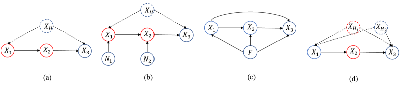
Figure 1: (a) The causal graph of the SCM considered in Example 2. (b) The corresponding auxiliary graph according to Definition 1. (c) The MAG of the augmented graph defined in (Jaber et al.,, 2020), which indicates the output of their algorithm. (d) The causal graph of an alternative SCM that has the same auxiliary graph.

Theorem 2.

In the presence of latent confounders and Assumption 2, the candidate intervention target set ${\bf K}$ returned by LIT algorithm is the set of observed variables that are children of ${\bf N}_{\bf T}$ in $Aux(G_{\bf T})$, i.e., ${\bf K}=\cup_{N_{i}\in{\bf N}_{\bf T}}Ch_{Aux(G_{\bf T})}(N_{i})$.

Theorem 2 gives a graphical characterization of the recovered candidate intervention set ${\bf K}$. In particular, according to Definition 1, ${\bf T_{O}}$ is a subset of ${\bf K}$. This is because the edge from $X_{i}\in{\bf T_{O}}$ to its corresponding exogenous noise $N_{i}$ in $G_{\bf T}$ is not removed. This means that LIT algorithm returns a superset of ${\bf T_{O}}$. Further, two other types of variables are added to ${\bf K}$ according to the conditions in part (a) and part (b) of Definition 1, respectively.

Remark 2.

We can make the following observations from Theorem 2. First, under the causal sufficiency assumption, Theorem 2 implies that ${\bf T_{O}}$ can be uniquely identified. This is because no edges are added to $Aux(G_{\bf T})$ compared with $G_{\bf T}$ according to Definition 1. Second, if all latent variables are not intervention targets (i.e., ${\bf T}={\bf T_{O}}$), then our identifiability result is stronger than the existing results in (Jaber et al.,, 2020; Varici et al.,, 2022). In particular, they showed that in this case, ${\bf T_{O}}$ can only be identified up to the neighbors of ${\bf N}_{{\bf T}}$ in the MAG corresponding to $G_{\bf T}$. We improve their results by adding part (a)(ii) in Definition 1, due to the recovery of $\tilde{{\bf N}}_{{\bf T}}$. See Example 2 below.

Example 2.

Consider the same example as in Example 1. Following the results in (Jaber et al.,, 2020; Varici et al.,, 2022), the MAG of the augmented graph defined in (Jaber et al.,, 2020) is shown in Figure 1(c). The recovery output of their algorithms is $\{X_{1},X_{2},X_{3}\}$ as all the observed variables are the neighbor of the $F$-node defined in their work. On the contrary, LIT algorithm has a more accurate recovery of the intervention targets. Specifically, the auxiliary graph is shown in Figure 1(b). The edge from $N_{1}$ to $X_{3}$ is not added since ${\bf I}_{1}\neq{\bf I}_{3}$ (which violates part (a)(ii) in Definition 1), and the edge from $N_{2}$ to $X_{3}$ is not added because there is no inducing path (which violates part (a)(i)). Therefore ${\bf K}=\{X_{1},X_{2}\}$, which is the same as the output in Example 1. Lastly, note that ${\bf K}$ is not always equal to ${\bf T_{O}}$. Consider the causal graph in Figure 1(d) where ${\bf T}=\{X_{H_{1}},X_{2}\}$. Its corresponding auxiliary graph is exactly the one in Figure 1(b). However, ${\bf T_{O}}=\{X_{2}\}\subsetneq\{X_{1},X_{2}\}={\bf K}$, and we cannot distinguish whether $X_{1}$ or $X_{H_{1}}$ is the intervention target.

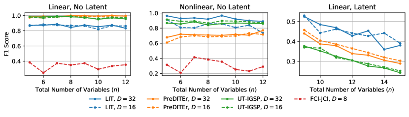
Figure 2: Comparison of LIT algorithm with previous work in locating intervention targets.

4 Experiments

We evaluated the performance of LIT algorithm on randomly generated models. We considered the following three settings, with different numbers of environments $D=\{8,16,32\}$ for data generation: (1) Linear Gaussian model under causal sufficiency assumption; (2) Nonlinear model under causal sufficiency assumption; (3) Linear Gaussian model in the presence of latent confounders. We considered the following methods in our empirical studies: 1- LIT (our proposed method); 2- PreDITEr algorithm (Varici et al.,, 2022) which allows for latent confounders (that are not in ${\bf T}$) but assumes the model to be linear; 3- UT-IGSP algorithm (Squires et al.,, 2020) which works for both linear and nonlinear SCMs under merely causal sufficiency; 4- FCI-JCI123 algorithm in (Mooij et al.,, 2020) which allows for both latent confounders and nonlinearity in the model.

We repeated each setting for 40 times, and reported the average F1-score in recovering ${\bf T}_{{\bf O}}$ for each setting. The results are shown in Figure 2. (Full experimental results can be found in Appendix E.) Note that FCI-JCI is executable only under the first two settings with $D=8$ due to huge run times. The results of other algorithms for $D=8$ are provided in Appendix E. In the first setting, as we expected, PreDITEr has the best performance as it is designed specifically for linear Gaussian SCMs. UT-IGSP and LIT algorithm have decent performances, while FCI-JCI123 does not perform well. In the second setting, LIT and UT-IGSP can both recover the intervention targets with high accuracy. On the contrary, the performance of PreDITEr becomes worse as it is not designed for nonlinear models. Finally, in the third setting, in the presence of latent confounders, the performance of UT-IGSP becomes much worse because it cannot handle any latent confounders. Meanwhile, LIT outperforms PreDITEr and UT-IGSP for various numbers of variables in the system. Note that the best F1-score that can be achieved by any algorithm is strictly less than one as there are intervention targets that can never be recovered. Lastly, we note that LIT algorithm significantly reduces the number of CI tests performed: LIT algorithm takes at most 80 CI tests while PreDITER requires up to 30000 PDE estimates. See Appendix E for more details.

5 Comparison with previous work

Learning causal structures in multi-environment setting with unknown target interventions has been the focus of several recent work. Under causal sufficiency assumption, Ghassami et al., (2017) considered linear SCMs in multi-environment setting and showed that the intervention targets can be recovered by checking whether the variances of residuals of some linear regressions are changing across the environments. Squires et al., (2020) proposed an algorithm to recover an interventional Markov equivalence class (I-MEC) from a collection of interventional distributions with unknown intervention targets. The proposed algorithm greedily searches over the space of permutations to minimize a score function. In computing the score function, it is required to perform invariance tests to check whether pairs of distributions are equal which is in general sample inefficient in practice. Brouillard et al., (2020) proposed a causal discovery algorithm that recovers the intervention targets by finding the optimal solution of an appropriately defined score function. In both (Squires et al.,, 2020; Brouillard et al.,, 2020), no interventions are allowed in the observational environment and therefore the algorithm must know which environment pertains to the observation-only setting. More recently, Perry et al., (2022) proposed a score-based approach based on sparse mechanism shift hypothesis and showed that it can recover the true causal graph up to an I-MEC. However, it has the same drawback of performing invariance tests as in (Squires et al.,, 2020).

In the presence of latent confounders, Jaber et al., (2020) defined $\Psi$-Markov property which connects the collection of interventional distributions in the multi-environment setting to a pair of a causal graph and set of intervention targets. Moreover, they proposed a sound and complete algorithm to learn the equivalence class of all pairs of graphs and intervention targets that are consistent with the interventional distributions. The proposed algorithm can be used to learn a superset of variables that are intervened between any pair of environments. If there is no latent confounder in the system, this algorithm recovers the true intervention targets. Similar to (Squires et al.,, 2020), the proposed algorithm requires performing invariance tests to check whether pairs of distributions are equal across environments. Moreover, it needs an exponentially growing number of conditional independence and invariance tests as the number of variables increases. Mooij et al., (2020) proposed a causal modeling framework that considers an auxiliary context variable for each environment and applies standard causal discovery algorithms (such as FCI) to learn the causal relationships among context variables and system variables. They provided graphical conditions to read off the intervention targets from the output of their algorithm.

All the aforementioned work learns the causal structure up to an equivalence class and identifies a candidate intervention set as a byproduct of the output of the causal discovery task. Very recently, Varici et al., (2022) proposed a method to learn merely intervention targets (rather than recovering the causal structure) in linear SCMs and it is more scalable than previous work as it does not perform extensive CI tests. Moreover, the identifiability result in recovering intervention targets is exactly the same as (Jaber et al.,, 2020). Note that all the previous work (Jaber et al.,, 2020; Mooij et al.,, 2020; Varici et al.,, 2022) assume that if latent confounders exist, none of them is in the intervention target set. We relax this assumption and allow latent confounders to be among the intervention targets.

6 Conclusions

We addressed the problem of identifying unknown intervention targets in a multi-environment setting. Our two-phase algorithm recovers the exogenous noises and matches them with corresponding endogenous variables. Under the causal sufficiency assumption, our algorithm uniquely identifies the intervention targets. In the presence of latent confounders, we provided a candidate intervention target set which is more informative than previous work. Experiment results support the advantages of the proposed algorithm in identifying intervention targets. As a future work, in the recovery phase, it is an interesting direction to strengthen the identifiability result of non-linear SCM with latent variables which would broaden the applicability of our method to more complex systems.

Appendix A Further discussion on the recovery phase

A.1 Detailed description about contrastive learning approach and nonlinear ICA

Nonlinear ICA refers to an instance of unsupervised learning, where the goal is to learn the independent components/features that generate multi-dimensional observed data. In particular, suppose that ${\bf X}=(X_{1},\cdots,X_{n})$, is a $n$-dimensional vector that is generated from $n$ independent components ${\bf N}=(N_{1},\cdots,N_{n})$. Let ${\bf g}:\mathbb{R}^{n}\rightarrow\mathbb{R}^{n}$ be a smooth and invertible function transforming the latent components (aka sources) to the observed data, i.e., ${\bf X}={\bf g}({\bf N})$. Function ${\bf g}$ is called the “mixing function”. The goal in nonlinear ICA is to recover the inverse function ${\bf g}^{-1}$ and also the latent components in ${\bf N}$.

We briefly describe the general approach in recent advances in nonlinear ICA (Hyvarinen et al.,, 2019; Khemakhem et al.,, 2020; Sorrenson et al.,, 2020) for the case where no additional assumptions are made about the class of mixing functions. The main idea is to exploit non-stationarity in the data to recover the independent components. In particular, each component $N_{i}$ depends on some auxiliary variable $U$ and it is independent of other components given $U$, i.e., $\log p({\bf N}|U)=\sum_{i}q_{i}(N_{i}|U),$ where $q_{i}$s are some functions. The auxiliary variable $U$ could be an index of a time segment or the index of some environments where we obtained samples from variables in ${\bf X}$. In this formulation, the distributions of components can change across the environments or time segments. It is often assumed that the distribution of each $N_{i}$ given $U$ is a member of the exponential family.

Definition 2.

A random variable $N_{i}$ belongs to the exponential family of order one given a random variable $U$ if its conditional probability distribution function (pdf) can be written as: $p(N_{i}|U)=\frac{Q_{i}(N_{i})}{Z_{i}(U)}\exp\left(\lambda_{i}(U)\tilde{q}_{i}(N_{i})\right)$ where $Q_{i}$, $Z_{i}$, $\lambda_{i}$s, and $\tilde{q}_{i}$s are some scalar-valued functions.

Example 3.

For $\tilde{q}_{i}(N_{i})=-N_{i}^{2}/2$, and $Q_{i}(N_{i})=1$, the above conditional pdf reduces to Gaussian whose variance is changing across the environments.

The general approach to exploit non-stationarity in data is to use contrastive learning to transform the unsupervised learning problem in nonlinear ICA to a supervised learning task. Specifically, a classifier is trained to discriminate samples of a real dataset from their randomized version, i.e., $\tilde{{\bf X}}=({\bf X},U)$ versus $\tilde{{\bf X}^{\prime}}=({\bf X},U^{\prime})$, where $U^{\prime}$ is drawn randomly from the distribution of $U$, which in practice can be obtained by randomized permutations of the samples of $U$.

In this approach, a nonlinear regression model is trained with the following form: $r({\bf X},U)={\bf h}({\bf X})^{T}{\bf v}(U)+a({\bf X})+b(U)$ where ${\bf h}({\bf X}):\mathbb{R}^{n}\rightarrow\mathbb{R}^{n}$, ${\bf v}(U):\mathbb{R}\rightarrow\mathbb{R}^{n}$, and $a,b$ are some scalar-valued functions. The model classifies a sample coming from the real data set with probability $1/(1+\exp(-r({\bf X},U)))$. It has been shown in several work such as in (Hyvarinen et al.,, 2019; Khemakhem et al.,, 2020) that if all the components are changed enough across the environments, then the independent components can be recovered from ${\bf h}({\bf X})$ up to some permutation and component-wise nonlinear transformation.

How constrastive learning approach above is applied in our work

As we have access to a collection of distributions in $\mathcal{P}$, we will exploit the heterogeneity in data to recover the exogenous noises in ${\bf N}_{{\bf T}}$. Let auxiliary variable $U$ denote the index of the environment and assume that the exogenous noises belong to the exponential family in Definition 2. Moreover, assume that $\lambda_{i}$s corresponding to any $N_{i}\in{\bf N}_{{\bf T}}$ are randomly generated across the environments and $\tilde{q}_{i}(N_{i})$s are strictly monotonic functions of $|N_{i}|$. We utilize a contrastive learning approach similar to what we discussed above. We train the nonlinear regression model $r({\bf O},U)={\bf h}({\bf O})^{T}{\bf v}(U)+a({\bf O})+b(U)$ with universal approximation capability for the supervised learning task of discriminating $({\bf O},U)$ from $({\bf O},U^{\prime})$ where ${\bf h}({\bf O}):\mathbb{R}^{|{\bf O}|}\rightarrow\mathbb{R}^{|{\bf O}|}$, ${\bf v}(U):\mathbb{R}\rightarrow\mathbb{R}^{|{\bf O}|}$, and $a({\bf O})$, $b(U)$ are some scalar-valued functions.

A.2 Additional discussion on Assumption 1

Assumption 1(a).

We provide two examples on when Assumption 1(a) is satisfied. Note that Assumption 1(a) requires that $|{\bf O}|=n=|{\bf X}|$, which indicates that the model is causally sufficient.

First, for linear SCMs, the structural equations can be written in vector form as ${\bf X}={\bf B}{\bf X}+{\bf N}$ where ${\bf B}$ is $n\times n$ matrix. Rewrite this equation as ${\bf X}=({\bf I}-{\bf B})^{-1}{\bf N}$. Therefore, the corresponding mixing function is given by $({\bf I}-{\bf B})^{-1}$ and the above assumption is satisfied if and only if ${\bf I}-{\bf B}$ is invertible, which is already satisfied when the causal graph is a DAG.

Second, for nonlinear SCMs, invertibility of the mixing function is satisfied when the model is an additive noise model, which can be written as $X_{i}=f_{i}(Pa_{i})+N_{i}$. In this case, the inverse function that maps ${\bf N}$ to ${\bf O}$ can be constructed according to the following equation: $N_{i}=X_{i}-f_{i}(Pa_{i})$. Note that the invertibility of the mixing function does not depend on $f_{i}$. This result can be generalized into the following remark:

Remark 3.

For a nonlinear SCM $X_{i}=f_{i}(Pa_{i},N_{i})$, Assumption 1(a) is satisfied if the model is acyclic, $f_{i}$ is continuous, and the partial derivative $\partial f_{i}/\partial N_{i}$ is strictly negative or positive for all $X_{i}\in{\bf X}$ and any values of $Pa_{i}$.

We note that the condition in Remark 3 can be satisfied when $f_{i}$ in the data generating model is designed as a multi-layer perceptron with ReLU activation function, where all model weights are positive.

Assumption 1(b).

For Assumption 1(b), we note that if the SCM is a linear non-Gaussian model, i.e., linear SCM with non-Gaussian exogenous noises, and latent confounders are present, then Assumption 1(b) implies that: (1) All intervention targets must be observed variables, i.e., ${\bf T}\subseteq{\bf O}$; and (2) Latent variables cannot have children in ${\bf T}$. In other words, ${\bf T}$ can only include observed variables that do not have latent parents. Please see Appendix D.2 for the proof. However, we observed experimentally that if the SCM is linear Gaussian within each environment, then we can recover the noises in ${\bf N}_{\bf T}$ while allowing latent confounders to be in ${\bf T}$ using linear ICA methods.

Appendix B Further discussion on the matching phase

B.1 Markov Property in the Augmented Graph

For the given SCM $\mathcal{M}$, we construct a modified version $\mathcal{\tilde{M}}_{{\bf T}}$ as follows. We add ${\bf N}_{{\bf T}}$ to the set of endogenous variables in $\mathcal{M}$ and remove them from the set of exogenous noises. Moreover, for any $X_{i}\in{\bf T}$, we change its structural assignment as follows: $X_{i}:=\tilde{f}_{i}(\tilde{P\!A}_{i})=f_{i}(P\!A_{i},N_{i})$ where $\tilde{f}_{i}$ is the new causal mechanism of relating it to its new set of parents $\tilde{P\!A}_{i}=P\!A_{i}\cup\{N_{i}\}$. For each variable $N_{i}\in{\bf N}_{{\bf T}}$, we add an exogenous noise to $\mathcal{\tilde{M}}_{{\bf T}}$ and set the value of $N_{i}$ to its corresponding exogenous noise. Please note that with this construction, the joint distribution over ${\bf X}$ entailed by SCM $\tilde{\mathcal{M}}_{{\bf T}}$ is exactly the same as the one entailed by original SCM $\mathcal{M}$. With the exact same argument in the proof of Theorem 1.4.1 in (Pearl,, 2009), it can be shown that the distribution $p({\bf X}\backslash{\bf T_{L}},{\bf N}_{{\bf T}})$ entailed by SCM $\tilde{\mathcal{M}}_{{\bf T}}$ satisfies the local Markov property as the value of each observed variable is uniquely determined given the values of its parts and the corresponding exogenous noise. Moreover, in causal DAGs, the local Markov property implies the Global Markov property (Geiger and Pearl,, 1990). Hence, the joint distribution $p({\bf X}\backslash{\bf T_{L}},{\bf N}_{{\bf T}})$ satisfies Markov property with respect to its corresponding causal graph, $G_{{\bf T}}$.

B.2 Example Explaining the Conditions under Causal Sufficiency Assumption

The following example illustrates how the the conditions in Proposition 2 can be used to recover ${\bf T}$.

Figure 3: An example of SCM: Intervention targets ${\bf T}=\{X_{1},X_{2},$ $X_{5}\}$ are shown by red circles.

Example 4.

Figure 3 depicts the augmented graph of an SCM in which ${\bf T}=\{X_{1},X_{2},X_{5}\}$ (indicated by red circles). In the recovery phase, we recover three noises $\tilde{N}_{1},\tilde{N}_{2},\tilde{N}_{5}$, which are invertible transformations of $N_{1}$, $N_{2}$, $N_{5}$, respectively. Note that we do not know the correspondence of the noises to the variables as there are permutation indeterminacy. The indicator sets for all the variables are: ${\bf I}_{1}=\{\tilde{N}_{1}\}$, ${\bf I}_{2}=\{\tilde{N}_{2}\}$, ${\bf I}_{3}=\{\tilde{N}_{1},\tilde{N}_{2}\}$, ${\bf I}_{4}=\emptyset$, ${\bf I}_{5}={\bf I}_{6}={\bf I}_{7}=\{\tilde{N}_{1},\tilde{N}_{2},\tilde{N}_{5}\}$. For $X_{1}$ and $X_{2}$, the condition in II is satisfied. Thus, they are in ${\bf T}$. As for $X_{3}$ and $X_{4}$, the condition in I holds and therefore they are not in ${\bf T}$. For the variables in $\{X_{5},X_{6},X_{7}\}$, the condition in 5 holds and the only variable satisfying the condition in (C1) is $X_{5}$ as $\tilde{N}_{5}$ is independent of $X_{6}$ and $X_{7}$ given ${\bf S}_{5}\cup\{X_{5}\}$ where ${\bf S}_{5}=\{X_{1},X_{2},X_{3},X_{4}\}$.

B.3 Definition of Auxiliary Graph

In this section we present the formal definition of auxiliary graph.

Definition 1 (Auxiliary graph).

For each variable $X_{i}$, denote ${\bf I}_{0}(X_{i})$ as $An_{G_{\bf T}}(X_{i})\cap{\bf N}_{\bf T}$. Given a SCM and its corresponding augmented graph $G_{\bf T}$, the auxiliary graph $Aux(G_{\bf T})$ is constructed from $G_{\bf T}$ as follows:

1. For each $X_{i}\in{\bf T_{O}}$ with its corresponding exogenous noise $N_{i}$, add the edge $N_{i}\rightarrow X_{j}$ if (i) there is an inducing path between them relative to ${\bf L}\setminus{\bf T_{L}}$ in $G_{\bf T}$ (i.e., there is an edge between $N_{i}$ and $X_{j}$ in the MAG corresponding to $G_{\bf T}$) , and (ii) ${\bf I}_{0}(X_{i})={\bf I}_{0}(X_{j})$.

2. (i) For each $N_{l}\in{\bf N}_{\bf T}$ (noise that corresponds to a variable in ${\bf T_{L}}$) and each of its child $X_{i}$, keep the edge $N_{l}\rightarrow X_{i}$ if for any other child $X_{j}$ of $N_{l}$ in $G_{\bf T}$, ${\bf I}_{0}(X_{i})\subseteq{\bf I}_{0}(X_{j})$. Otherwise remove the edge $N_{l}\rightarrow X_{i}$. (ii) For each remaining edge $N_{l}\rightarrow X_{i}$, add (remove) the edge $N_{l}\rightarrow X_{k}$ if there is an (no) inducing path between $X_{k}$ and all (some) parents of $X_{i}$ in ${\bf N}_{\bf T}$ relative to ${\bf L}\setminus{\bf T_{L}}$ in $G_{\bf T}$, and ${\bf I}_{0}(X_{k})={\bf I}_{0}(X_{i})$.

Recall from Section 3.3.1 that under Assumption 2, $An_{G_{\bf T}}(X_{i})\cap{\bf N}_{\bf T}$ can be recovered by ${\bf I}_{i}$. Therefore we use ${\bf I}_{0}(X_{i})$ to represent the true value of ${\bf I}_{i}$ which does not depend on the recovery output. Further, it is noteworthy that while part (b)(ii) in Definition 1 includes both adding and removing of the edges, the addition or removal of edges in the step is independent of the order of the edge selection $N_{l}\rightarrow X_{i}$.

Appendix C Efficient algorithm based on mixing matrix

We show that the problem of locating the intervention targets in the causally sufficient systems can be reduced to the problem of causal discovery on linear SCMs with deterministic relations (Yang et al., 2022a, ; Yang et al., 2022b, ). This allows us to design a more efficient algorithm based on existing causal discovery algorithms for linear SCMs. In the following, we first show that there is a connection between the indicator set $\mathcal{I}$ and the mixing matrix of a linear SCM. Next, we present an alternative algorithm of LIT under causal sufficiency based on existing algorithms, and analyze its computational complexity. Lastly, we extend the algorithm to the case with latent confounders.

To show these connection between the two problems, we define a mapping $\phi$ from the set of SCMs with soft interventions and the set of linear SCMs with deterministic relations, where for each SCM $\mathcal{M}$ with intervention target set ${\bf T}$, $\phi(\mathcal{M},{\bf T})$ is constructed as follows. Each variable $X$ in $\mathcal{M}$ is mapped to a non-deterministic variable, denoted by $\phi(X)$, if $X\in{\bf T}$, and is mapped to a deterministic variable if it is not in ${\bf T}$. Further, for each pair of variables $(X_{i},X_{j})$ in $\mathcal{M}$, $\phi(X_{i})$ is a parent of $\phi(X_{j})$ in $\phi(\mathcal{M})$ with coefficient 1 if and only if $X_{i}$ is a parent of $X_{j}$ in $\mathcal{M}$. The following proposition states that the indicator set of $\mathcal{M}$ is the same as the support of the mixing matrix of $\phi(\mathcal{M},{\bf T})$.

Proposition 4.

For a given SCM $\mathcal{M}$ with intervention target set ${\bf T}$, we denote the $(i,j)$-th entry of the mixing matrix of $\phi(\mathcal{M},{\bf T})$ as $w_{ij}$. Then for all $i\in[n]$ and $j\in[|{\bf T}|]$, $w_{ij}\neq 0$ if and only if $\tilde{N}_{j}\in{\bf I}_{i}$.

Remark 4.

Proposition 4 implies that if the underlying model is linear Gaussian, then under Assumption 2, the indicator set can be obtained from the recovered mixing matrix in linear ICA.

Example 5.

Consider SCM $\mathcal{M}$ over a collider structure: $X_{1}\rightarrow X_{3}\leftarrow X_{2}$, where $X_{1}$ and $X_{2}$ are intervention targets with corresponding exogenous noises $\tilde{N_{1}}$ and $\tilde{N_{2}}$, respectively. The indicator sets are: ${\bf I}_{1}=\{\tilde{N}_{1}\}$, ${\bf I}_{2}=\{\tilde{N}_{2}\}$, and ${\bf I}_{3}=\{\tilde{N}_{1},\tilde{N}_{2}\}$. Under the mapping $\phi$, $\mathcal{M}$ is mapped to the linear SCM $\mathcal{M}^{\prime}$ over the same collider structure, where $\phi(X_{3})$ is a deterministic variable, and $\phi(X_{1}),\phi(X_{2})$ are non-deterministic. The mixing matrix corresponding to $\mathcal{M}^{\prime}$ is ${\bf W}=[1\;0;\;0\;1;\;1\;1]$, where for all $i=1,2,3$, ${\bf I}_{i}$ represents the support of the $i$-th row of ${\bf W}$.

Proposition 4 implies that any recovery algorithm for linear SCMs with deterministic relations, that are based on the mixing matrix, can be applied to our problem. In particular, Yang et al., 2022a considered the problem of causal discovery on linear SCMs with measurement error, which can be considered as a special case of deterministic relations. They proposed AOG recovery algorithm, where the input is the mixing matrix, and the output is a partition of the variables into distinct sets such that variables in the same set has the same row support. Note that the conditions in I and II in Proposition 2 is purely based on indicator set, and the condition 5 is based on partitioning variables based on the indicator set.

We devise a more efficient version of the LIT algorithm in Algorithm 2 which utilizes AOG recovery algorithm. Specifically, instead of iterating over all variables, Algorithm 2 iterates over the recovered noises, which corresponds to the non-empty residual sets $\mathcal{N}_{i}$ in Proposition 2. (Recall that under causal sufficiency assumption, $|\mathcal{N}_{i}|=1$ if it is not empty.) During each iteration, the algorithm finds a row $X_{i}$ with only one non-zero entry and has the smallest corresponding value in $\mathbf{n}$. Note that this entry corresponds to the noise in $\mathcal{N}_{i}$, and for any variable $X_{j}$ that has the same support on the submatrix as $X_{i}$, if the number in $\mathbf{n}$ corresponding to $X_{j}$ is larger than the number corresponding to $X_{i}$, then ${\bf I}_{i}$ is unique and $X_{i}$ satisfies condition II. Moreover, ${\bf I}_{i}$ is a strict subset of ${\bf I}_{j}$ and thus $X_{i}\in{\bf S}_{j}$. Please note that $X_{j}$ satisfies the condition in I since the union of the indicator sets for $X_{i}$ and a subset of selected variables in the previous loops is equal to ${\bf I}_{j}$. Therefore, $X_{j}$ should be excluded from ${\bf T}$. Otherwise, if the number in $\mathbf{n}$ corresponding to $X_{j}$ is equal to the number corresponding to $X_{i}$, then ${\bf I}_{i}={\bf I}_{j}$, and we need to use (C1) to find the variable in ${\bf K}$.

To show that Algorithm 2 is a more efficient version of Algorithm 1, note that the first step of Algorithm 1 is to compute ${\bf S}_{i}$ for all observed variables $X_{i}$. Since ${\bf S}_{i}$ involves pairwise comparison of the indicator sets, the time complexity of this step is $\Theta(n^{2}|T|)$, where $n$ is the number of observed variables, and $|{\bf T}|$ is the number of recovered exogenous noises. On the contrary, Algorithm 2 does not need to calculate all ${\bf S}_{i}$. It is only needed when we need to check (C1). Since all variables in $\mathcal{X}_{i}$ have the same indicator set, finding ${\bf S}_{i}$ takes at most $\Theta(n|{\bf T}|^{2})$. It can be shown that the time complexity for Algorithm 1 is $\Theta(n^{2}|{\bf T}|)$, as the conditions in I and II are hard to check and each takes $\Theta(n^{2}|{\bf T}|)$ time. On the contrary, the time complexity for Algorithm 2 is $\Theta(n|{\bf T}|^{2})$.

1 Obtain $\tilde{{\bf N}}_{\bf T}$ and $\mathcal{I}$ from data. Rewrite $\mathcal{I}$ into the matrix form, where each row represents an indicator set. Denote it as ${\bf I}$.

2 Calculate the number of non-zero entries in each row of $\mathbf{I}$. Denote the vector of these numbers as $\mathbf{n}$, where each entry in $\mathbf{n}$ corresponds to a row in $\mathbf{I}$.

3 Initialize $\tilde{\mathbf{I}}=\mathbf{I}$, ${\bf K}\leftarrow\emptyset$.

4 Remove all rows in $\tilde{\mathbf{I}}$ with no non-zero entry.

5 while $\tilde{\mathbf{I}}$ is not empty do

6       Find a row in $\tilde{\mathbf{I}}$ that contains only one non-zero entry, and has the smallest corresponding value in $\mathbf{n}$. If there are multiple such rows, randomly select one. Denote the selected row as $\mathbf{w}$, and its corresponding value in $\mathbf{n}$ as $n_{0}$.

7       Consider the rows in $\tilde{\mathbf{I}}$ with the same support (non-zero entry) as $\mathbf{w}$, including $\mathbf{w}$ itself. Denote the set of variables that correspond to these rows as $\mathcal{Z}_{I}$.

8       Denote the set of variables in $\mathcal{Z}_{I}$ with the same corresponding value as $n_{0}$ in $\mathbf{n}$ as $\mathcal{Z}_{J}$.

9       if $\mathcal{Z}_{J}$ has only one element then

10             Add the variable that corresponds to $\mathbf{w}$ to ${\bf K}$.

11            

12      else

13             Find the only variable $X_{i_{k}}$ in $\mathcal{Z}_{J}$ that satisfies (C1); ${\bf K}\leftarrow{\bf K}\cup\{X_{i_{k}}\}$.

14            

15      Remove from $\tilde{\mathbf{I}}$ the rows corresponding to the variables in $\mathcal{Z}_{I}$, and the column containing the corresponding non-zero entries in these rows.

16      

return ${\bf K}$

Algorithm 2 Locating interventions target (LIT) algorithm under causal sufficiency.

Lastly, we can extend Algorithm 1 to the case in the presence of latent confounders. The new algorithm is shown in Algorithm 3. In particular, in order to check IV, we count the number of non-zero entries in each column, and check IV in lines 8-11, which is also a condition that is purely based on the indicator sets.

1 Obtain $\tilde{{\bf N}}_{\bf T}$ and $\mathcal{I}$ from data and rewrite $\mathcal{I}$ into the matrix form ${\bf I}$.

2 Calculate the number of non-zero entries in each row and each column of $\mathbf{I}$. Denote the vector of these numbers as $\mathbf{n}$ and $\mathbf{m}$, where each entry in $\mathbf{n}$ corresponds to a row in $\mathbf{I}$, and each entry in $\mathbf{m}$ corresponds to a column in $\mathbf{I}$.

3 Initialize $\tilde{\mathbf{I}}=\mathbf{I}$, ${\bf K}\leftarrow\emptyset$.

4 Remove all rows in $\tilde{\mathbf{I}}$ with all entry being zero.

5 while $\tilde{\mathbf{I}}$ is not empty do

6       Find a row in $\tilde{\mathbf{I}}$ that contains the fewest number of non-zero entry, and has the smallest corresponding value in $\mathbf{n}$. If there are multiple such rows, randomly select one. Denote the selected row as $\mathbf{w}$, the variable corresponding to this row as $X_{w}$, and the corresponding value in $\mathbf{n}$ as $n_{0}$.

7       Consider the rows in $\tilde{\mathbf{I}}$ with the same support (non-zero entry) as $\mathbf{w}$, including $\mathbf{w}$ itself. Denote the set of variables that correspond to these rows as $\mathcal{Z}_{I}$, and the the noise terms corresponding to the support of $\mathbf{w}$ as $\mathcal{N}_{I}$.

8       Denote the set of variables in $\mathcal{Z}_{I}$ with corresponding value $n_{0}$ in $\mathbf{n}$ as $\mathcal{Z}_{J}$, and the set of noise terms in $\mathcal{N}_{I}$ with the smallest corresponding value in $\mathbf{m}$ as $\mathcal{N}_{J}$.

9       Randomly select one noise term $N_{m}$ in $\mathcal{N}_{J}$. Consider the submatrix of $\mathbf{I}$ where the rows correspond to the (column) support of $N_{m}$, and the columns correspond to the (row) support of $X_{w}$.

10       if This submatrix includes any zero entry then

11            pass

12      else

13             if $|\mathcal{Z}_{J}|>1$ then

14                   Find the set of variables in $\mathcal{Z}_{J}$ that satisfy (C2). Denote it as $\mathcal{Z}_{K}$.

15                   $\mathcal{Z}_{J}\leftarrow\mathcal{Z}_{J}\setminus\mathcal{Z}_{K}$.

16                  

17            ${\bf K}\leftarrow{\bf K}\cup\mathcal{Z}_{J}$.

18            

19      Remove from $\tilde{\mathbf{I}}$ the rows corresponding to the variables in $\mathcal{Z}_{I}$, and the columns corresponding to the noise terms in $\mathcal{N}_{I}$.

20      

return ${\bf K}$

Algorithm 3 LIT algorithm in the presence of latent confounders.

Appendix D Proofs

D.1 Proof of Proposition 1

We first prove the statement of proposition for the case of ${\bf L}=\emptyset$. With infinite samples and a model with universal approximation capability, after training, the regression model will equal the difference of the log-densities in the two classes:

$$\begin{split}r({\bf X},U)&=\log p({\bf N},U)+\log|{\bf J}{\bf g}({\bf X})|-\log p({\bf N})-\log p(U)-\log|{\bf J}{\bf g}({\bf X})|\\ &=\log p({\bf N}|U)-\log p({\bf N})\\ &=\sum_{i}\log Q_{i}(N_{i})-\log Z_{i}(U)+\tilde{q}_{i}(N_{i})\lambda_{i}(U)-\log p({\bf N}).\end{split}$$ (1)

If we consider the form of $r({\bf X},U)={\bf h}({\bf X})^{T}{\bf v}(U)+a({\bf X})+b(U)$ for $r({\bf X},U)$, we can set the functions ${\bf h}({\bf X})$, ${\bf v}(U)$, $a({\bf X})$, and $b(U)$ such that it is equal to the right hand side of above equation. In particular, we can have the following equality

$$\sum_{i}h_{i}({\bf X})v_{i}(U)+a({\bf X})+b(U)=\sum_{i}\log Q_{i}(N_{i})-\log Z_{i}(U)+\sum_{i}\tilde{q}_{i}(N_{i})\lambda_{i}(U)-\log p({\bf N}),$$ (2)

with the following possible solution:

$$\begin{split}h_{i}({\bf X})=\tilde{q}_{i}(N_{i}),v_{i}(U)=\lambda_{i}(U),a({\bf X})=\sum_{i}\log Q_{i}(N_{i})-\log p({\bf N}),b(U)=-\sum_{i}\log Z_{i}(U).\end{split}$$ (3)

The random variable $U$ is equal to $d$, if the sample is drawn from the environment $E_{d}$ where $1\leq d\leq D$. Let ${\bf P}$ be $D\times n$ matrix where $d$-th row is equal to $[\lambda_{1}(d),\cdots,\lambda_{n}(d)]$. We collect $\tilde{q}_{i}$s in the vector $\tilde{{\bf q}}({\bf N})=[\tilde{q}_{1}(N_{1}),\cdots,\tilde{q}_{n}(N_{n})]^{T}$. We also define the matrix ${\bf V}$ where $d$-th row is equal to $[v_{1}(d),\cdots,v_{n}(d)]$. Finally, we collect $-\sum_{i}\log Z_{i}(U)-b(U)$ for different values of $U$ in a vector ${\bf Z}$. Based on these definitions, we have:

$${\bf V}{\bf h}({\bf X})={\bf P}\tilde{{\bf q}}({\bf N})+{\bf Z}+\mathbf{1}\left(\sum_{i}\log Q_{i}(N_{i})-\log p({\bf N})-a({\bf X})\right),$$ (4)

where $\mathbf{1}$ is a $D\times 1$ vector of all ones. If from both sides of the above equation, we subtract the first row from the others,

$${\bf V}^{\prime}{\bf h}({\bf X})={\bf P}^{\prime}\tilde{{\bf q}}({\bf N})+{\bf Z}^{\prime},$$ (5)

where ${\bf V}^{\prime},{\bf P}^{\prime}$, and ${\bf Z}^{\prime}$ denote the resulting matrices after subtraction corresponding to ${\bf V},{\bf P},$ and ${\bf Z}$, respectively.

The columns corresponding to exogenous noises that are not changing across environments are zeros in ${\bf P}^{\prime}$. Thus, we can remove these columns from ${\bf P}^{\prime}$ and also the corresponding entries in $\tilde{{\bf q}}({\bf N})$. We denote the resulting matrix and vector by ${\bf P}^{\prime\prime}$ and $\tilde{{\bf q}}({\bf N}_{{\bf T}})$, respectively. Hence, we can rewrite the above equation as follows:

$${\bf V}^{\prime}{\bf h}({\bf X})={\bf P}^{\prime\prime}\tilde{{\bf q}}({\bf N}_{{\bf T}})+{\bf Z}^{\prime}.$$ (6)

As $\lambda_{i}(U)$s are generated randomly across the environments and $D\geq|{\bf T}|+1$, ${\bf P}^{\prime\prime}$ is full column rank with measure one. Therefore, we have:

$$\tilde{{\bf q}}({\bf N}_{{\bf T}})=({\bf P}^{\prime\prime})^{\dagger}{\bf V}^{\prime}{\bf h}({\bf X})-{\bf Z}^{\prime\prime},$$ (7)

where $({\bf P}^{\prime\prime})^{\dagger}$ is pseudo-inverse of matrix ${\bf P}^{\prime\prime}$ and ${\bf Z}^{\prime\prime}=({\bf P}^{\prime\prime})^{\dagger}{\bf Z}^{\prime}$. Since we know that the entries of $\tilde{{\bf q}}({\bf N}_{{\bf T}})$ are linearly independent, $({\bf P}^{\prime\prime})^{\dagger}{\bf V}^{\prime}$ is full row rank. Moreover, $q_{i}(N_{i})$s are non-Gaussian as they are bounded from above to ensure integrability. Thus, we can recover $\tilde{{\bf q}}({\bf N}_{{\bf T}})$ from ${\bf h}({\bf X})$ by solving an under-complete linear ICA problem.

Now, let us assume that there are some latent variables in the system, i.e., ${\bf L}\neq\emptyset$. As we know that there exists an invertible function $\tilde{{\bf g}}$ such that $\tilde{{\bf g}}({\bf O})=({\bf N}_{{\bf T}},{\bf V})$, we have:

$$\begin{split}r({\bf O},U)&=\log p({\bf O},U)-\log p({\bf O})-\log p(U)\\ &=\log p({\bf O}|U)-\log p({\bf O})\\ &=\log p({\bf N}_{{\bf T}},{\bf V}|U)+\log|{\bf J}\tilde{{\bf g}}({\bf O})|-\log p({\bf N}_{{\bf T}},{\bf V})-\log|{\bf J}\tilde{{\bf g}}({\bf O})|\\ &=\log p({\bf N}_{{\bf T}}|U)-\log p({\bf N}_{{\bf T}}),\end{split}$$ (8)

where the third equality is due to the existence of invertible function $\tilde{{\bf g}}$ and the last equality is according to the assumptions that ${\bf N}_{{\bf T}}\perp\!\!\!\perp{\bf V}|U$, ${\bf V}\perp\!\!\!\perp U$. Please note that these two assumptions imply that ${\bf N}_{{\bf T}}\perp\!\!\!\perp{\bf V}$. Similar to the causally sufficient case, based on the form of $r({\bf O},U)$, we can write the following equation:

$$\sum_{j}h_{j}({\bf O})v_{j}(U)+a({\bf O})+b(U)=\sum_{i:X_{i}\in{\bf T}}\log Q_{i}(N_{i})-\log Z_{i}(U)+\tilde{q}_{i}(N_{i})\lambda_{i}(U)-\log p({\bf N}_{{\bf T}}).$$ (9)

where $h({\bf O}):\mathbb{R}^{|{\bf O}|}\rightarrow\mathbb{R}^{|{\bf O}|}$. Let ${\bf M}$ be $D\times|{\bf T}|$ matrix where $d$-th row is equal to $[\lambda_{1}(d),\cdots,\lambda_{|{\bf T}|}(d)]$. We collect $\tilde{q}_{i}$s in the vector $\tilde{{\bf q}}({\bf N}_{{\bf T}})$. We also define the matrix ${\bf W}$ where $d$-th row is equal to $[v_{1}(d),\cdots,v_{|{\bf O}|}(d)]$. Finally, we collect $-\sum_{i:X_{i}\in{\bf T}}\log Z_{i}(U)-b(U)$ for different values of $U$ in a vector ${\bf Z}$. Based on these definitions, we have:

$${\bf W}{\bf h}({\bf O})={\bf M}\tilde{{\bf q}}({\bf N}_{{\bf T}})+{\bf Z}+\mathbf{1}\left(\sum_{i:X_{i}\in{\bf T}}\log Q_{i}(N_{i})-\log p({\bf N}_{{\bf T}})-a({\bf O})\right),$$ (10)

where $\mathbf{1}$ is a $D\times 1$ vector of all ones.

Now, if from both sides of the above equation, we subtract the first row from the others, we have

$${\bf W}^{\prime}{\bf h}({\bf O})={\bf M}^{\prime}\tilde{{\bf q}}({\bf N}_{{\bf T}})+{\bf Z}^{\prime},$$ (11)

where ${\bf V}^{\prime},{\bf L}^{\prime}$, and ${\bf Z}^{\prime}$ denote the resulting matrices after subtraction corresponding to ${\bf W},{\bf M},$ and ${\bf Z}$, respectively.

As $\lambda_{i}(U)$s are generated randomly across the environments and $D\geq|{\bf T}|+1$, ${\bf M}^{\prime}$ is full column rank with measure one. Therefore, we have:

$$\tilde{{\bf q}}({\bf N}_{{\bf T}})=({\bf M}^{\prime})^{\dagger}{\bf W}^{\prime}{\bf h}({\bf O})-{\bf Z}^{\prime\prime},$$ (12)

where $({\bf M}^{\prime})^{\dagger}$ is pseudo-inverse of matrix ${\bf M}^{\prime}$ and ${\bf Z}^{\prime\prime}=({\bf M}^{\prime})^{\dagger}{\bf Z}^{\prime}$. Since we know that the entries of $\tilde{{\bf q}}({\bf N}_{{\bf T}})$ are linearly independent, $({\bf M}^{\prime\prime})^{\dagger}{\bf W}^{\prime}$ is full row rank. Moreover, $q_{i}(N_{i})$s are non-Gaussian as they are bounded from above to ensure integrability. Thus, we can recover $\tilde{{\bf q}}({\bf N}_{{\bf T}})$ from ${\bf h}({\bf O})$ by solving an under-complete linear ICA problem.

So far, we showed that the recovery phase can be performed up to some component-wise nonlinear transformation (not necessarily an invertible one). However, similar to Corollary 2 in (Hyvarinen and Morioka,, 2016), it can be shown that from $\tilde{{\bf q}}({\bf N}_{{\bf T}})$ and the observed vector ${\bf O}$, the exogenous noises in ${\bf N}_{{\bf T}}$ can be recovered up to some strictly monotonic transformation if each function $\tilde{q}_{i}(N_{i})$ is a strictly monotonic function of $|N_{i}|$.

D.2 Regarding Assumption 1(b) on Linear non-Gaussian Models

In the following we prove that, in the linear non-Gaussian model (i.e., linear SCM with non-Gaussian exogenous noises) with the causal graph $G$, if ${\bf L}\neq\emptyset$, then the conditions in Proposition 1 imply that: (i) ${\bf T}\subseteq{\bf O}$; (ii) For each latent variable $H_{i}\in{\bf L}$, $Ch_{G}(H_{i})\cap{\bf T}=\emptyset$, i.e., $H_{i}$ cannot have children in ${\bf T}$ where $Ch_{G}(H_{i})$ is the children of $H_{i}$.

The linear SCM has the following matrix form:

$${\bf L}={\bf N}_{\bf L};\quad{\bf O}={\bf A}{\bf O}+{\bf A}^{\prime}{\bf L}+{\bf N}_{\bf O},$$ (13)

where ${\bf N}_{\bf L}$ and ${\bf N}_{\bf O}$ represent the vector of exogenous noises associated with latent and observed variables, respectively. We also denote the exogenous noises whose distributions are not changing across the environments by ${\bf N}_{{\bf T}^{c}}$. ${\bf A}$ represents the direct causal relationships among observed variables and ${\bf A}^{\prime}$ represents the direct causal relations from latent to observed variables. Note that if we permute the variables such that ${\bf X}=[{\bf L},{\bf O}]$, then the adjacency matrix ${\bf B}$ after the same (row and column) permutation is $[\mathbf{0},\mathbf{0};{\bf A}^{\prime},{\bf A}]$. Under the acyclicity assumption, ${\bf A}$ can be permuted into a strictly lower triangular matrix. Following (13), ${\bf O}$ can be written as a linear combination of the noise terms in $({\bf N}_{\bf L},{\bf N}_{\bf O})$:

$${\bf O}=[{\bf D}\quad{\bf C}]\begin{bmatrix}{\bf N}_{\bf L}\\ {\bf N}_{\bf O}\end{bmatrix},$$ (14)

where ${\bf D}=({\bf I}-{\bf A})^{-1}{\bf A}^{\prime}$ and ${\bf C}=({\bf I}-{\bf A})^{-1}$. Denote ${\bf W}=[{\bf D}\quad{\bf C}]$, which represents the total causal effects (i.e., sum of product of path coefficients) among variables (Spirtes et al.,, 2000). If all exogenous noises are non-Gaussian and no two columns of ${\bf W}$ are linearly dependent of each other, then ${\bf W}$ can be recovered up to permutation and scaling of the columns using overcomplete ICA. Given that some variables in ${\bf X}$ belong to ${\bf T}$, we can rewrite (14) as follows:

$${\bf O}=[{\bf W}_{{\bf T}}\quad{\bf W}_{{\bf T}^{c}}]\begin{bmatrix}{\bf N}_{{\bf T}}\\ {\bf N}_{{\bf T}^{c}}\end{bmatrix},$$ (15)

where ${\bf W}_{{\bf T}}$ and ${\bf W}_{{\bf T}^{c}}$ represent the submatrix of ${\bf W}$ that correspond to the exogenous noises in ${\bf N}_{{\bf T}}$ and ${\bf N}_{{\bf T}^{c}}$, respectively.

If the conditions in Proposition 1 hold, then there exists an invertible matrix ${\bf G}$, such that

$${\bf G}{\bf O}=[{\bf G}{\bf W}_{{\bf T}}\quad{\bf G}{\bf W}_{{\bf T}^{c}}]\begin{bmatrix}{\bf N}_{{\bf T}}\\ {\bf N}_{{\bf T}^{c}}\end{bmatrix}=\begin{bmatrix}{\bf N}_{{\bf T}}\\ {\bf V}\end{bmatrix}.$$ (16)

Partition ${\bf G}$ into $[{\bf G}_{1};{\bf G}_{2}]$, where ${\bf G}_{1}\in\mathbb{R}^{|{\bf T}|\times n}$ represent the first $|{\bf T}|$ rows of ${\bf G}$, and ${\bf G}_{2}\in\mathbb{R}^{(n-|{\bf T}|)\times n}$ represent the remaining rows. Therefore, according to (16), we have

$${\bf G}_{1}{\bf W}_{{\bf T}}{\bf N}_{{\bf T}}+{\bf G}_{1}{\bf W}_{{\bf T}^{c}}{\bf N}_{{\bf T}^{c}}={\bf N}_{{\bf T}}.$$ (17)

We first show that if all noises in ${\bf N}_{{\bf T}}$ and ${\bf N}_{{\bf T}^{c}}$ are mutually independent and non-Gaussian, then (17) implies that ${\bf G}_{1}{\bf W}_{{\bf T}}={\bf I}$, and ${\bf G}_{1}{\bf W}_{{\bf T}^{c}}=\mathbf{0}$. This is because for each noise $N_{i}\in{\bf N}_{{\bf T}}$, $i\in[|{\bf T}|]$, according to (17), $N_{i}$ can be written as a linear combination of exogenous noises in ${\bf N}_{{\bf T}}\cup{\bf N}_{{\bf T}^{c}}$. Since all noises are mutually independent and non-Gaussian, according to Darmois-Skitovitch theorem (Darmois,, 1953; Skitovitch,, 1953), the coefficient of any $N_{j}$, $j\neq i$ on $N_{i}$ must be zero. Otherwise $N_{j}$ and $N_{i}$ are independent, but

For each exogenous noise $N\in{\bf N}_{{\bf T}}\cup{\bf N}_{{\bf T}^{c}}$, denote its corresponding column vector in ${\bf W}$ in (15) as ${\bf w}_{N}$. Then ${\bf G}_{1}{\bf W}_{{\bf T}}={\bf I}$, ${\bf G}_{1}{\bf W}_{{\bf T}^{c}}=\mathbf{0}$ is equivalent to: For each exogenous noise $N$ and its corresponding column vector ${\bf w}_{N}$, ${\bf G}_{1}{\bf w}_{N}=\mathbf{0}$ if $N\in{\bf N}_{{\bf T}^{c}}$, and ${\bf G}_{1}{\bf w}_{N}={\bf e}_{N}$ if $N\in{\bf N}_{{\bf T}}$, where ${\bf e}_{N}$ is the basis (one-hot) vector where the entry corresponding to $N$ is one and the rest are zero. Further, for each latent variable $H_{i}\in{\bf L}$, we have

$${\bf w}_{N_{H_{i}}}=\sum_{j:X_{j}\in Ch_{G}(H)}a^{\prime}_{ji}{\bf w}_{N_{X_{j}}},$$

where $a^{\prime}_{ji}$ represent the $(j,i)$-th entry of matrix ${\bf A}^{\prime}$ in (13). This is because for any observed variable $X\in{\bf O}$, the total causal effect of $H_{i}$ on $X$ can be written as summation of the total causal effect from each child of $H_{i}$ to $X$ multiplied by the direct causal effect from $H_{i}$ to this child (i.e., $a^{\prime}_{ji}$). Therefore, we have

$${\bf G}_{1}{\bf w}_{N_{H_{i}}}=\sum_{j:X_{j}\in Ch_{G}(H_{i})}a^{\prime}_{ji}{\bf G}_{1}{\bf w}_{N_{X_{j}}}.$$ (18)

Since ${\bf G}_{1}{\bf w}_{N}$ corresponds to either zero vector or basis vector, and different noises in ${\bf N}_{\bf T}$ correspond to different basis vectors, (18) implies that ${\bf G}_{1}{\bf w}_{N_{H_{i}}}=\mathbf{0}$, and ${\bf G}_{1}{\bf w}_{N_{X_{j}}}=\mathbf{0}$ for all latent variable $H_{i}\in{\bf L}$, and all $X_{j}\in Ch_{G}(H_{i})$. This means that ${\bf T}$ only includes observed variables that do not have latent parents.

D.3 Proof of Proposition 2

Consider any recovered noise $\tilde{N}_{i}\in\tilde{\mathbf{N}}_{{\bf T}}$. Without loss of generality, suppose that $\tilde{N}_{i}$ corresponds to $X_{i}$. We first show that $\tilde{N}_{i}$ only depends on the descendants of $X_{i}$. First, for any node $X_{j}\in Des(X_{i})$, the path $N_{i}\rightarrow X_{i}\rightarrow\cdots\rightarrow X_{j}$ in graph $G_{{\bf T}}$ is not blocked without conditioning on any other variable and $\tilde{N}_{i}\not\!\perp\!\!\!\perp X_{j}$. Moreover, for any $X_{j}$ which is a non-descendent of $X_{i}$, there is always a collider on any path between $X_{j}$ and $N_{i}$ and thus it is blocked. Hence, we have: $\tilde{N}_{i}\!\perp\!\!\!\perp X_{j}$.

Remark 5.

Based on what we proved above, we can imply that ${\bf I}_{i}$ contains only the noises in $\tilde{{\bf N}}_{{\bf T}}$ whose corresponding variables are ancestors of $X_{i}$.

Remark 6.

For any two variables $X_{i},X_{j}$, if we have ${\bf I}_{j}\subsetneq{\bf I}_{i}$ , then $X_{j}$ cannot be a descendent of $X_{i}$. Since if $X_{j}$ is a descendent of $X_{i}$, then based on Remark 5, we can conclude that ${\bf I}_{i}\subseteq{\bf I}_{j}$ which violates our assumption.

Now, we prove the three statements in the proposition based on the above two remarks:

I By contradiction, suppose that $X_{i}$ is in ${\bf T}$. If for a variable $X_{j}$, we have ${\bf I}_{j}\subsetneq{\bf I}_{i}$, then based on Remark 6, it cannot be a descendent of $X_{i}$. Now if the condition in I satisfies, then there exists a set such as ${\bf I}_{j}$, where $j\in{\bf S}_{i}$, such that $i\in{\bf I}_{j}$. But according to Remark 5, this means that $X_{j}$ is a descendant of $X_{i}$ which is a contradiction.

II As the condition in I is not satisfied, there exists $k$ such that $\tilde{N}_{k}\in\mathcal{N}_{i}={\bf I}_{i}\backslash\cup_{j:X_{j}\in{\bf S}_{i}}{\bf I}_{j}$. Suppose that $\tilde{N}_{k}$ corresponds to $X_{k}$. Based on Remark 5, $X_{k}$ should be an ancestor of $X_{i}$. Moreover, we have ${\bf I}_{k}\subseteq{\bf I}_{i}$. As ${\bf I}_{i}$ is unique, then ${\bf I}_{k}\subsetneq{\bf I}_{i}$ and $X_{k}\in{\bf S}_{i}$. This contradictsthe fact that $\tilde{N}_{k}\in{\bf I}_{i}\backslash\cup_{j:X_{j}\in{\bf S}_{i}}{\bf I}_{j}$ and the proof is complete.

5 As the indicator sets do not satisfy the condition in I, $\mathcal{N}_{i}$ is not empty. Suppose that $\tilde{N}_{k}\in\mathcal{N}_{i}$ and $\tilde{N}_{k}$ corresponds to $X_{k}$. We know that $X_{k}$ should be in the set $\{X_{i_{1}},\cdots,X_{i_{p}}\}$. Otherwise, based on Remark 5, ${\bf I}_{k}\subseteq{\bf I}_{i_{1}}$. Now, if ${\bf I}_{k}\subsetneq{\bf I}_{i_{1}}$, then $X_{k}\in{\bf S}_{i_{1}}$ which is a contradiction. Thus, ${\bf I}_{k}$ should be equal to ${\bf I}_{i}$ but in that case $X_{k}$ is in the set $\{X_{i_{1}},\cdots,X_{i_{p}}\}$. Thus, we can conclude that at least one of the variables in this set is in ${\bf T}$. Please note that at most one of the variable in $\{X_{i_{1}},\cdots,X_{i_{p}}\}$ can be in ${\bf T}$. Otherwise, the variables in this set cannot have the same indicator set. Therefore, exactly one of the variables in $\{X_{i_{1}},\cdots,X_{i_{p}}\}$ is in ${\bf T}$ and we can obtain the corresponding recovered noise by ${\bf I}_{i_{1}}\backslash\cup_{j:X_{j}\in{\bf S}_{i_{1}}}{\bf I}_{j}$. Without loss of generality, suppose that $X_{i_{1}}\in{\bf T}$. Then, based on Remark 5, other variables in $\{X_{i_{1}},\cdots,X_{i_{p}}\}$ should be descendant of $X_{i_{1}}$. The set ${\bf S}_{i_{1}}$ contains the ancestors of $X_{i_{1}}$. Thus, it also includes parents of $X_{i_{1}}$. Now, for any path between $N_{i_{1}}$ and $X_{i_{j}}$, $j\geq 2$, if it is outgoing from node $X_{i_{1}}$, then it is blocked by $X_{i_{1}}$. If it is in-going toward $X_{i_{1}}$, then it is blocked by a parent of $X_{i_{1}}$ which is inside the set ${\bf S}_{i_{1}}$. Thus, under T-faithfulness assumption, it implies that $\tilde{N}_{i_{1}}\perp\!\!\!\perp X_{i_{j}}|\{X_{i_{1}}\}\cup{\bf S}_{i_{1}},\mbox{ for all }2\leq j\leq p$. Please note that the variables in $\{X_{i_{2}},\cdots,X_{i_{p}}\}$ cannot satisfy the condition in 5 as they cannot block the path $N_{i_{1}}\rightarrow X_{i_{1}}$ by any set ${\bf S}_{i_{j}}$ for $j\geq 2$ and the proof is complete.

D.4 Proof of Theorem 1

It can be easily seen that for any variable $X_{i}\in{\bf X}$, only one of the conditions in I-5 in Proposition 2 is satisfied. Moreover, these conditions cover all possible cases regarding the relation of the set $\cup_{j:X_{j}\in{\bf S}_{i}}{\bf I}_{j}$ and ${\bf I}_{i}$ and also the uniqueness of ${\bf I}_{i}$ in $\mathcal{I}$. Furthermore, in either case, we know definitely whether $X_{i}$ is in ${\bf T}$ or not. Thus, the intervention target ${\bf T}$ can be identified uniquely by checking these three conditions for any variable $X_{i}\in{\bf X}$ and the proof is complete.

D.5 Proof of Theorem 2

To better distinguish between intervention targets in ${\bf T_{O}}$ and in ${\bf T_{L}}$, we use $\tilde{N}_{h_{i}}$ to represent the exogenous noise corresponding to $X_{i}$ for all $X_{i}\in{\bf T_{L}}$. For ease of notation, we denote the true noises $N_{j}$ in the augmented graph as $\tilde{N}_{j}$ in the following proof, since there is a one-to-one correspondence between them. We first present the following remark:

Remark 7.

If a group of variables $\mathcal{X}_{i}=\{X_{i_{1}},\cdots,X_{i_{p}}\}$ have the same indicator set and $\mathcal{N}_{i}\neq\emptyset$ (note that $\mathcal{N}_{i_{k}}$ is the same for all $k\in[p]$), then any root variable in $\mathcal{X}_{i}$ (i.e., variable with no parent in $\mathcal{X}_{i}$) must be a child of all recovered noises in $\mathcal{N}_{i_{1}}$.

D.5.1 Proof of sufficiency

We show that if an observed variable $X_{i}$ is a child of some noise $\tilde{N}_{j}\in\tilde{{\bf N}}_{\bf T}$ in $Aux(G_{\bf T})$, then it is included in the output ${\bf K}$ of the LIT algorithm. We consider each of the following four cases:

1. $X_{i}\in{\bf T}$.

2. $X_{i}\not\in{\bf T}$, and $\tilde{N}_{j}$ is the exogenous noise of some observed variable $X_{j}$.

3. $X_{i}\not\in{\bf T}$, $\tilde{N}_{j}$ is the exogenous noise of some latent confounder $H_{j}$, and $H_{j}$ is a parent of $X_{i}$ in $G$.

4. $X_{i}\not\in{\bf T}$, $\tilde{N}_{j}$ is the exogenous noise of some latent confounder $H_{j}$, and $H_{j}$ is not a parent of $X_{i}$ in $G$.

In the following we show that, under each of these four cases, $X_{i}$ is included in the output ${\bf K}$. That is, $X_{i}$ violates the condition in I, violates the condition in IV, and either satisfies the condition in II or violates (C2) in C2. Note that the conditions in II and in C2 only depends on the uniqueness of the indicator set, therefore we do not need to check II.

Case (i). If $X_{i}\in{\bf T}$, then its corresponding exogenous noise $\tilde{N}_{i}$ satisfies $i\in\tilde{N}_{i}$. Therefore the condition in I Proposition 2 is not satisfied. Further, any observed variable $X_{j_{l}}$ with $i\in{\bf I}_{j_{l}}$ must be a descendant of $X_{i}$, and hence satisfies ${\bf I}_{i}\subseteq{\bf I}_{j_{l}}$. Therefore the condition in IV is not satisfied. Lastly, if there are no other variables that have the same indicator set, then $X_{i}\in{\bf K}$ according to II. Otherwise, all other variables that have the same indicator set as ${\bf I}_{i}$ must be descendants of $X_{i}$ (because of $\tilde{N}_{i}$), hence $X_{i}$ is a child of any recovered noise in $\mathcal{N}_{i}$ (according to Remark 7). Therefore there does not exist $l$ such that (C2) holds, which means that $X_{i}\in{\bf K}$.

Case (ii). If $X_{i}\not\in{\bf T}$ and $\tilde{N}_{j}$ is the exogenous noise of some observed variable $X_{j}$, then ${\bf I}_{j}={\bf I}_{i}$, and there is at least one inducing path from $\tilde{N}_{j}$ to $X_{i}$. This means that any variable $X_{k}\in{\bf S}_{i}$ is not a descendant of $\tilde{N}_{j}$ in $G_{{\bf T}}$, which implies that $j\in{\bf I}_{i}$ but not in $\cup_{j^{\prime}:X_{j^{\prime}}\in{\bf S}_{i}}{\bf I}_{j^{\prime}}$. Therefore the condition in I is not satisfied. Next, note that $j\in\mathcal{N}_{i}=\mathcal{N}_{j}$, ${\bf I}_{i}={\bf I}_{j}$, and (A) in IV does not hold for $X_{j}$ (explained in Case (i)). Therefore (A) in IV does not hold for $X_{i}$ either.

Lastly, note that there is at least one other variable ($X_{j}$) that has the same indicator set as $X_{i}$, and $X_{j}$ is a root variable in $\mathcal{X}_{i}$ (following the same argument as in Case (i)). Therefore $X_{j}$ is directly connected to all recovered noises in $\mathcal{N}_{i}$. Since $\tilde{N}_{j}$ is only directly connected to $X_{j}$, this means that if there is an inducing path from $\tilde{N}_{j}$ to $X_{i}$, then for any $l\in\mathcal{N}_{i}$, by changing the first edge on this path from $\tilde{N}_{j}\rightarrow X_{j}$ to $\tilde{N}_{l}\rightarrow X_{j}$, the new path is also an inducing path from $\tilde{N}_{l}$ to $X_{i}$. Therefore there does not exist $l$ such that (C2) holds, which means that $X_{i}\in K$.

Case (iii). If $X_{i}\not\in{\bf T}$, $\tilde{N}_{j}$ is the exogenous noise of latent confounder $H_{j}$, and $H_{j}$ is a parent of $X_{i}$ in $G$, then according to Definition 1, for all other children $X_{k}$ of $H_{j}$, we have ${\bf I}_{i}\subseteq{\bf I}_{k}$. This immediately implies that the condition in IV is not satisfied. This also implies that for any variable $X_{k^{\prime}}\in{\bf S}_{i}$, $j\not\in{\bf I}_{k^{\prime}}$. Therefore, we have $j\in{\bf I}_{i}$ but not in $\cup_{j^{\prime}:X_{j^{\prime}}\in{\bf S}_{i}}{\bf I}_{j^{\prime}}$, which means that the condition in I is not satisfied. Lastly, if ${\bf I}_{i}$ is unique, then $X_{i}\in{\bf K}$. Otherwise, since there is an inducing path from all recovered noises in $\mathcal{N}_{i}$ to $X_{i}$, there does not exist $l$ such that (C2) holds. Therefore $X_{i}\in{\bf K}$.

Case (iv). If $X_{i}\not\in{\bf T}$, $\tilde{N}_{j}$ is the exogenous noise of latent confounder $H_{j}$, and $H_{j}$ is not a parent of $X_{i}$ in $G$, then according to Definition 1, there exists some $X_{k}$ such that $H_{j}$ is directly connected to $X_{k}$, and ${\bf I}_{k}={\bf I}_{i}$. Further, there is an inducing path from $\tilde{N}_{j}$ to $X_{i}$. Note that all children of $\tilde{N}_{j}$ after part (b) have the same indicator set, which is the same as ${\bf I}_{i}$. Therefore the condition in I does not hold. Further, since the condition in (A) does not hold for $X_{k}$ (explained in Case (iii)) and ${\bf I}_{k}={\bf I}_{i}$, the condition in (A) does not hold for $X_{i}$ either. Lastly, since there is an inducing path from all recovered noises in $\mathcal{N}_{i}$ to $X_{i}$, there does not exist $l$ such that (C2) holds. Therefore $X_{i}\in{\bf K}$.

Conclusion: We show that if an observed variable $X_{i}$ belongs to $\cup_{\tilde{N}_{i}\in\tilde{{\bf N}}_{\bf T}}Ch_{Aux(G_{\bf T})}(\tilde{N}_{i})$, i.e., it is a child of some noise $\tilde{N}_{j}\in\tilde{{\bf N}}_{\bf T}$ in $Aux(G_{\bf T})$, then it is included in the output ${\bf K}$ of the LIT algorithm.

D.5.2 Proof of necessity

We show that if an observed variable $X_{i}$ is included in the output ${\bf K}$ of the LIT algorithm, then it must be a child of some noise $\tilde{N}_{j}\in\tilde{{\bf N}}_{\bf T}$. That is, if $X_{i}$ violates the condition in I (i.e., $\mathcal{N}_{i}\neq\emptyset$), and the condition in IV, and either:

1. ${\bf I}_{i}$ is unique, or

2. ${\bf I}_{i}$ is not unique, and among all variables with the same indicator set, the condition in (C2) does not hold for $X_{i}$,

then it must be a child of some noise $\tilde{N}_{j}\in\tilde{{\bf N}}_{\bf T}$.

Case (i). If ${\bf I}_{i}$ is unique. This implies that any recovered noise $\tilde{N_{j}}\in\mathcal{N}_{i}$ is a parent of $X_{i}$ in $G_{\bf T}$. This is because otherwise the child of $\tilde{N_{j}}$ is a ancestor of $X_{i}$ but does not belong to ${\bf S}_{i}$. Hence it has the same indicator set as ${\bf I}_{i}$, which violates the uniqueness of ${\bf I}_{i}$.

Consider all these recovered noises $\tilde{N_{j}}\in\mathcal{N}_{i}$. If there exists $\tilde{N_{j}}$ such that $X_{i}$ is the only child of $\tilde{N_{j}}$, then $\tilde{N}_{j}$ is the exogenous noise of $X_{i}$, i.e., $X_{i}\in{\bf T_{O}}$, which is a subset of $\cup_{\tilde{N}_{i}\in\tilde{{\bf N}}_{\bf T}}Ch_{Aux(G_{\bf T})}(\tilde{N}_{i})$. Otherwise, if all noises $\tilde{N_{j}}$ has at least two children, then all of them correspond to the exogenous noises of latent confounders. Since the condition in IV is violated, there exist $l\in\mathcal{N}_{i}$ such that for all $j_{l}$ with $l\in{\bf I}_{j_{l}}$, ${\bf I}_{i}\subseteq{\bf I}_{j_{l}}$. This implies that the indicator set of any other child of $\tilde{N}_{l}$ in $G_{\bf T}$ must be a (strict) superset of $X_{i}$. Therefore the edge $\tilde{N}_{l}\rightarrow X_{i}$ is kept according to part (b)(i) of Definition 1, i.e., $X_{i}$ is the child of $\tilde{N}_{l}$ in $Aux(G_{\bf T})$.

Case (ii). If ${\bf I}_{i}$ is not unique. This means that $\mathcal{X}_{i}$ is not a singleton. Consider the root variables in $\mathcal{X}_{i}$. Note that following the induced causal order induced on $\mathcal{X}_{i}$, there is at least one root variable. If $X_{i}$ is a root variable, then according to Remark 7, all recovered noises in $\mathcal{N}_{i}$ is a parent of $X_{i}$ in $G_{\bf T}$. In this case we can apply the same proof as in Case (i) to show that $X_{i}$ is a child of some $\tilde{N}_{j}$ in $Aux(G_{\bf T})$. That is, if there exists $\tilde{N_{j}}$ such that $X_{i}$ is the only child of $\tilde{N_{j}}$, then $X_{i}\in{\bf T_{O}}$. Otherwise, if all noises $\tilde{N_{j}}$ has at least two children, then since the condition in IV is violated, part (b)(i) in Definition 1 is satisfied, and there is an inducing path from all recovered noises in $\mathcal{N}_{i}$ to $X_{i}$ (because a direct connection is an inducing path). Therefore $X_{i}$ is the child of all $\tilde{N}_{j}$ in $Aux(G_{\bf T})$.

Next, we consider the case if $X_{i}$ is not a root variable. If there exists $\tilde{N}_{j}\in\mathcal{N}_{i}$ such that it has only one direct child $X_{k}$ in $G_{\bf T}$, then $X_{k}$ is a root variable in $\mathcal{X}_{i}$. Since (C2) does not hold for $X_{i}$, this means that $\tilde{N}_{j}$ is not independent of $X_{i}$, conditioned on all observed ancestors of $X_{i}$ in $G_{\bf T}$ (i.e., $An_{G_{\bf T}}(X_{i})\setminus(\{X_{i}\}\cup({\bf L}\backslash{\bf T}))$). This is because all observed ancestors of $X_{i}$ in $G_{\bf T}$ must belong to one of the three following cases: observed variable whose indicator set is a strict subset of ${\bf I}_{i}$ (i.e., belongs to ${\bf S}_{i}$), observed variable whose indicator set is the same as ${\bf I}_{i}$ (i.e., belongs to $\mathcal{X}_{i}$), and the recovered exogenous noise of a latent confounder (i.e., belongs to $\cup_{l^{\prime}\in{\bf I}_{i_{1}}\setminus\{j\}}~{}\tilde{N}_{l^{\prime}}$).

In the following we show that the path that cannot be blocked by these observed ancestors is an inducing path. Suppose the path $\tilde{N}_{j}\rightarrow X_{k}\relbar\mkern-9.0mu\relbar V_{k_{1}}\relbar\mkern-9.0mu\relbar V_{k_{2}}\cdots X_{i}$ is not blocked, where $\{V_{k_{m}}\}$ are variables in $G_{\bf T}$, and $\relbar\mkern-9.0mu\relbar$ represents either $\leftarrow$ or $\rightarrow$. Note that $X_{k}$ is an ancestor of $X_{i}$ thus it is in the condition set. Therefore $X_{k}$ is a collider on this path, and we have the edge $X_{k}\leftarrow V_{k_{1}}$. This means that $V_{k_{1}}$ is a non-collider on this path and an ancestor of $X_{i}$ in $G_{\bf T}$. Since the path is active, $V_{k_{1}}$ is a latent confounder that is not changing across environments (i.e., belongs to ${\bf L}\setminus{\bf T}$). Therefore there is an edge $V_{k_{1}}\rightarrow V_{k_{2}}$. Next consider $V_{k_{2}}$. If $V_{k_{2}}$ is a non-collider and is not in the conditioning set (i.e., not an ancestor of $X_{i}$), then there is an edge $V_{k_{2}}\rightarrow V_{k_{3}}$. Since $V_{k_{2}}$ is not an ancestor of $X_{i}$, neither is $V_{k_{3}}$. Therefore $V_{k_{3}}$ is also a non-collider and we have $V_{k_{3}}\rightarrow V_{k_{4}}$. Repeat the same analysis on $V_{k_{m}}$ for all $m=4,5,\cdots$, the path is $\tilde{N}_{j}\rightarrow X_{k}\leftarrow V_{k_{1}}\rightarrow V_{k_{2}}\rightarrow V_{k_{3}}\rightarrow\cdots\rightarrow X_{i}$. This violates the claim that $V_{k_{2}}$ is not an ancestor of $X_{i}$. Therefore, $V_{k_{2}}$ is a collider and is in the conditioning set (i.e., an ancestor of $X_{i}$). Then we have the edge $V_{k_{2}}\leftarrow V_{k_{3}}$, and following the same analysis in $V_{k_{1}}$ on $V_{k_{3}}$, we have $V_{k_{3}}\in{\bf L}\setminus{\bf T}$ and is a confounder. Repeat the same analysis on $V_{k_{m}}$ for all $m=3,4,5,\cdots$, we have that variables $V_{k_{m}}$ are either confounders in ${\bf L}\setminus{\bf T}$, or colliders that are ancestors of $X_{i}$. Therefore this path is an inducing path from $\tilde{N}_{j}$ to $X_{i}$. According to part (a) in Definition 1, $X_{i}$ is the child of $\tilde{N}_{j}$ in $Aux(G_{\bf T})$.

Next, we consider the case when each recovered noise $\tilde{N}_{j}\in\mathcal{N}_{i}$ has at least two children in $G_{\bf T}$. Similar to the above argument, there is at least one root variable $X_{k}$ in $\mathcal{X}_{i}$ that is an ancestor of $X_{i}$. This means that ${\bf I}_{k}={\bf I}_{i}$, and the edge cannot be removed in part (b)(ii) in Definition 1. Further, for each recovered noise $\tilde{N}_{j}\in\mathcal{N}_{i}$, since (C2) does not hold for $X_{i}$, $\tilde{N}_{j}$ is not independent of $X_{i}$, conditioned on all observed ancestors of $X_{i}$ in $G_{\bf T}$. This means that there is a path from $\tilde{N}_{j}$ to $X_{i}$ that is not blocked by the observed ancestors. Similar to the argument above, suppose the path $\tilde{N}_{j}\rightarrow V_{k_{1}}\relbar\mkern-9.0mu\relbar V_{k_{2}}\cdots X_{i}$ is not blocked. If $V_{k_{1}}$ is a non-collider and is not an observed ancestor of $X_{i}$ (i.e., not in the conditioning set), then there is an edge $V_{k_{1}}\rightarrow V_{k_{2}}$, and $V_{k_{2}}$ is not an ancestor of $X_{i}$ either. This means that $V_{k_{2}}$ is also a non-collider and there is an edge $V_{k_{2}}\rightarrow V_{k_{3}}$. Repeat the same analysis on $V_{k_{m}}$ for all $m=3,4,5,\cdots$, the path is $\tilde{N}_{j}\rightarrow V_{k_{1}}\rightarrow V_{k_{2}}\rightarrow V_{k_{3}}\rightarrow\cdots\rightarrow X_{i}$. This violates the claim that $V_{k_{2}}$ is not an ancestor of $X_{i}$. Therefore, $V_{k_{1}}$ is a collider and is an ancestor of $X_{i}$. Then we can repeat the same analysis as above to conclude that this path is an inducing path. Therefore, there is an inducing path from each recovered noise $\tilde{N}_{j}\in\mathcal{N}_{i}$ to $X_{i}$, hence $X_{i}$ is a child of $\tilde{N}_{j}$ in $Aux(G_{\bf T})$, according to part (b)(ii) in Definition 1.

Conclusion: We show that if an observed variable $X_{i}$ is included in the output ${\bf K}$ of the LIT algorithm, then it must be a child of some recovered noise in $Aux(G_{\bf T})$, hence belongs to $\cup_{\tilde{N}_{i}\in\tilde{{\bf N}}_{\bf T}}Ch_{Aux(G_{\bf T})}(\tilde{N}_{i})$.

D.6 Proof of Remark 2

Regarding the equivalency between the condition (C2) and the condition (C1) under causal sufficiency assumption, note that under causal sufficiency assumption, the condition in (C2) can be rewritten as follows:

• Let $\mathcal{X}_{i}=\{X_{i_{1}},\cdots,X_{i_{p}}\}$, for some $p\geq 2$, be a set of all variables whose corresponding indicator sets are the same as $X_{i}$ and $\mathcal{N}_{i}\neq\emptyset$. Then for each $j\in[p]$, $X_{i_{j}}\not\in{\bf K}$ if and only if the following condition holds:

  $$\exists K\subseteq[p]\setminus\{j\},~{}\exists{\bf S}\subseteq{\bf S}_{i_{1}},~{}\text{ s.t. }\tilde{N}_{l}\perp\!\!\!\perp X_{i_{j}}|\left(\cup_{k^{\prime}\in K}X_{i_{k^{\prime}}}\right)\cup{\bf S}.$$ (C2)

Please note that $\mathcal{N}_{i}$ only contains $\tilde{N}_{l}$ under causal sufficiency assumption (otherwise, at least two variables are descendants of each other which is impossible) and each recovered noise only has one child (i.e., their corresponding intervention target) and cannot block any path. Moreover, for any $X_{i_{j}}$, the set $K=\{i_{k}\}$ and ${\bf S}={\bf S}_{i_{1}}$ is enough to guarantee that $\tilde{N}_{l}\perp\!\!\!\perp X_{i_{j}}|X_{i_{k}}\cup{\bf S}_{i_{1}}$ where $X_{i_{k}}\in{\bf T}$ and $\tilde{N}_{l}$ is its corresponding recovered noise. Thus, all $X_{i_{j}}$ with $j\neq k$ are excluded from ${\bf K}$. Moreover, $X_{i_{k}}$ is added to ${\bf K}$ as $\tilde{N}_{l}$ is the direct parent of $X_{i_{k}}$ and cannot be d-separated by a subset of observed variables and recovered noises.

About comparing our result with (Jaber et al.,, 2020) In the case that ${\bf T}_{{\bf O}}={\bf T}$, the augmented graph in (Jaber et al.,, 2020) is constructed as follows (which we show it by $G^{\prime}_{{\bf T}}$). For any pairs of environments such as $E_{i}$ and $E_{j}$, a node denoted by $F_{ij}$ is added to the original graph, and it is connected to all variables in ${\bf T}_{{\bf O}}$. Please note that in our setting, all variables in ${\bf T}$ are changing across the environments and all $F_{ij}$s are directly connected to ${\bf T}_{{\bf O}}$. The candidate set in (Jaber et al.,, 2020) is the set of neighbors of $F$-nodes in the MAG of the augmented graph. Now, based on Theorem 2, it is just needed to show that if some $\tilde{N}_{i}$ is a parent of some $X_{j}$ in $Aux(G_{\bf T})$, then some $F$-node is also connected to $X_{j}$ in MAG of $G^{\prime}_{{\bf T}}$. If $X_{j}$ is ${\bf T}_{{\bf O}}$, this is trivial as it should be connected to some recovered noise in $Aux(G_{\bf T})$ and also to some $F$-node in the MAG of $G^{\prime}_{{\bf T}}$. Thus, suppose that the $X_{i}\not\in{\bf T}_{{\bf O}}$. In that case, based on part (a)(i) of Definition 1, there should be an inducing path between $\tilde{N}_{i}$ and $X_{j}$ relative to ${\bf L}$ in $G_{{\bf T}}$. This path starts from $\tilde{N}_{i}$ and goes directly to its corresponding observed variable in ${\bf T}_{{\bf O}}$ (without loss of generality, let us say $X_{i}$) and continues until getting to $X_{j}$ in the augmented graph $G_{\bf T}$. Note that since there are no changing latent variables, this path only involves variables in ${\bf O}$ and ${\bf L}$. Therefore we can construct the same path on the original graph $G$. We denote the part of this path in the original graph by $P$. Now, in $G^{\prime}_{{\bf T}}$, due to symmetry among $F$-nodes, consider any of them. This node is connected to $X_{i}$ as $X_{i}\in{\bf T}$. Now, the path starting from the $F$-node and then going directly to $X_{i}$ and continuing based on $P$ until reaching $X_{j}$ is also an inducing path in $G^{\prime}_{{\bf T}}$. This shows that our identifiability result is stronger than the one in (Jaber et al.,, 2020) when ${\bf T}_{{\bf O}}={\bf T}$, because of part (a)(ii) in Definition 1.

Appendix E Experiment details

E.1 Simulation settings

Data Generating Mechanism. We evaluated the performance of LIT algorithm on randomly generated synthetic models. Specifically, we considered each of the three settings below for data generating mechanism:

1. Linear Gaussian model under causal sufficiency assumption: We randomly generated a directed acyclic graph with $n$ variables, where each edge is connected with probability 1.5/($n-1$). Further, we randomly selected $\lfloor(n+1)/2\rfloor$ variables to be the intervention targets set ${\bf T}$, and collected data from $D$ environments. For each variable $X_{i}\in{\bf T}$, in the first half of the environment, we sampled the variance of corresponding exogenous Gaussian noise in each environment from the uniform distribution on $[1,5]$. In the second half of the environments, we sampled the variance from the uniform distribution on $[5,9]$. For each variable $X_{i}\in{\bf X}\setminus{\bf T}$, we sampled the corresponding noise variance from the uniform distribution on $[1,3]$ (note that this is the same across all environments). The coefficients (edge weights) in the linear SCM are randomly sampled from the uniform distribution on $[0.5,1]$. We generated $5000$ number of samples in each environment.

2. Nonlinear model under causal sufficiency assumption: The generating mechanisms for the causal graph, the intervention targets and the noise variances are the same as Setting (1). We used Laplace noise as the exogenous noises. For each variable $X_{i}$, the function $f_{i}(\cdot)$ is a multi-layer perception (MLP) with one hidden layer, where the weights and biases are randomly selected between 0.5 and 1, and the activation function is LeakyReLU with negative slope $k=0.2$. Recall from Appendix A that the data generating model satisfies Assumption 1(a). We generated 3000 number of samples in each environment.

3. Linear Gaussian model in the presence of latent confounders: We randomly generated a directed acyclic graph with $n$ variables, where $\lfloor n/2\rfloor$ variables are latent variables, and each edge is connected with probability 1.5/($n-1$). We ensured that each latent variable has at least two observed children. Further, we randomly select $\lfloor n/2\rfloor$ variables to be the intervention target set ${\bf T}$, where 80% of the latent variables are in ${\bf T}$. We used Gaussian noise as the exogenous noises, and the selection of the noise variances are the same as Setting (1). We generated 5000 number of samples in each environment.

The number of environments $D$ was set to $\{8,16,32\}$ for all three settings.

Implementation of LIT Algorithm. For the recovering phase, in linear models (i.e., Setting (1) and (3)), we used FastICA Hyvärinen et al., (2001) to recover the noises. We pruned the entries in the mixing matrix with absolute value lass than 0.2, and consider the support of the pruned mixing matrix as the indicator set. In nonlinear models (i.e., Setting (2)), we ran a contrastive-learning approach similar to TCL Hyvarinen and Morioka, (2016), where we trained a four-layer MLP for label classification, and then applied FastICA on the input of the final layer to obtain $\tilde{{\bf N}}_{\bf T}$ (up to certain transformation). Note that we assume that we know the number of non-Gaussian components in all three settings. For recovering the indicator set, for each pair of recovered noise $\tilde{N}_{j}$ and observed variable $X_{i}$, we calculate the correlation between $\tilde{N}_{j}$ and $X_{i}$ within each environment, and take the sum over all environments as the overall correlation $\rho_{ij}$. We put $j\in{\bf I}_{i}$ if and only if $|\rho_{ij}|\geq 0.2$.

For the matching phase, for causally sufficient models (i.e., Setting (1) and (2)) we use Algorithm 2 to find ${\bf K}$. Regarding the CI test in (C1), for each variable $X_{i_{k}}\in\mathcal{X}_{i_{[p]}}$, we compute the sum of the partial correlation between $\tilde{N}_{l}$ and $X_{i_{j}}$ (conditioning on $X_{i_{j}}$ and ${\bf S}_{i_{1}}$) for all $j\neq k$. We then consider the variable $X_{i_{k}}$ with the smallest of such sum as the intervention target. For the case with latent confounders (i.e., Setting (3)), we use Algorithm 3 to find ${\bf K}$. We use a relaxed version of condition (C2), where we only performed the test for ${\bf S}={\bf S}_{i_{1}}$ and $K=[p]\setminus\{k\}$ for each $X_{i_{k}}$. We use partial correlation test with significance level 0.15.

Baseline methods. We compared the performance of LIT algorithm with the following methods:

1. PreDITEr algorithm in (Varici et al.,, 2022). The algorithm returns the same candidate intervention set as in (Jaber et al.,, 2020) in linear Gaussian SCMs. The algorithm allows for the presence of latent confounders (that are not intervention targets), but assumes the model to be linear Gaussian.

2. UT-IGSP algorithm in (Spirtes et al.,, 2000). The algorithm works for both linear and nonlinear SCMs. However, no latent confounders are allowed in the algorithm.

3. FCI-JCI123 algorithm in (Mooij et al.,, 2020). The algorithm returns a subset of intervention targets in the presence of latent confounders, where no latent variable can be in ${\bf T}$. Further, the algorithm does not require any assumption on the functional form.

We note that FCI-JCI123 algorithm is executable only under the first two settings with $D=8$ due to huge runtime. Therefore we only report FCI-JCI123 algorithm in these two setups. We fine-tuned all three algorithms with different confidence thresholds (parameters), and report the performance of both algorithms with the best performance (PreDITEr with threshold 0.05, UT-IGSP with threshold 0.005, and FCI-JCI123 with threshold 0.2).

There exists some other related work such $\psi$-FCI algorithm in (Jaber et al.,, 2020) which returns a candidate intervention in the presence of latent confounders or DCDI algorithm in (Brouillard et al.,, 2020) which returns an interventional MEC under causal sufficiency assumption. Regarding $\psi$-FCI algorithm, the current implementation is limited to discrete variables in graphs with a few variables. Moreover, the implementation of DCDI with unknown intervention targets is merely for hard interventions. Thus, we did not compare with these algorithms as their implementations cannot be used in our setting.

Metrics. We compared the recovered intervention targets ${\bf K}$ with the true intervention targets ${\bf T_{O}}$ based on the following metrics:

• Precision: The percentage of the element in ${\bf K}$ that is also in ${\bf T_{O}}$;

• Recall: The percentage of the element in ${\bf T_{O}}$ that is correctly recovered in ${\bf K}$;

• F1 Score: The harmonic mean of Precision and Recall.

Additionally, to evaluate how many CI/invariance tests can be reduced by LIT algorithm, we compared the number of CI tests conducted by LIT algorithm, and the number of precision difference estimations (PDE estimates) in PreDITEr algorithm, which are used to replace invariance tests in their algorithm (Varici et al.,, 2022). We note that in linear SCMs (i.e., settings 1 and 3), as explained in Appendix C, the indicator set $\mathcal{I}$ can be deduced from the recovered mixing matrix from linear ICA. Therefore we only reported the number of CI tests in (C1) (resp. (C2)) in condition 5 (resp. C2) for both settings.

E.2 Simulation results

Linear Gaussian model under causal sufficiency assumption. We selected $n=[5,6,7,8,9,10,$ $11,12]$ and $D=[8,16,32]$. We repeated the simulation for 40 times for each $n$ and $D$. We calculated the mean and the errorbar of the metrics, where the errorbar is defined as the 25% and 75% percentile among all 40 samples. The plots are shown in Figure 4. The rows represent different number of environments $D$ (32, 24, 8), and the columns represent different metrics (F1 score, precision, recall). We observe that PreDITEr algorithm has the best performance, where the $F1$ score is almost one. We note that this is because PreDITEr algorithm is designed specifically for intervention target estimation in linear Gaussian SCMs, which utilizes the sample covariance matrix in the recovery. Besides, UT-IGSP algorithm and LIT algorithm also have decent performances in this setup. Lastly, we observe that the performance of FCI-JCI123 is significantly worse than the other three methods. We note that the simulation results in Varici et al., (2022); Mooij et al., (2020) show that FCI-JCI has comparable performance when the intervention affects the noise distribution to have a mean shift. However, in our setting, the intervention only affects the noise distribution to have a changing variance (scale).

Nonlinear model under causal sufficiency assumption. We selected $n=[5,6,7,8,9,10,$ $11,12]$ and $D=[8,16,32]$, and also repeated the simulation for 40 times for each $n$ and $D$. The average of the metrics are shown in Figure 5. We observe that the performance of PreDITEr algorithm is worse than in Figure 4. This implies that the performance of PreDITEr algorithm depends heavily on the linear Gaussian assumption of the underlying model. Further, LIT algorithm and UT-IGSP algorithms have similar performance, where LIT performs better when the number of environment is large. This is because the number of environments has a significant impact on the recovery of the noises in nonlinear ICA. Lastly, FCI-JCI123 still have the worst performance.

Linear Gaussian model in the presence of latent confounders. We selected $n=[9,10,11,12,13,14,15]$ and $D=[8,16,32]$. We repeated the simulation for 40 times for each $n$ and $D$, and the average of the metrics are shown in Figure 6. Note that there are no error bars for recall, because all three high values in recall, and the 25% percentile is the same as the 75% percentile (i.e., 1.0) for all three algorithms (i.e., the recall on at least 30 out of 40 randomly generated graphs are one).

We observe that LIT algorithm has the best performance among all three algorithms. In particular, all three algorithms have high value in recall, and LIT algorithm has the highest precision. This means that all three algorithms can recover the intervention target in ${\bf T_{O}}$. However, since UT-IGSP algorithm does not allow for any latent confounders, and PreDITEr algorithm only allows for latent confounders that are not in ${\bf T}$, both algorithms cannot distinguish between a changing latent confounder and a changing observed variable. On the contrary, LIT algorithm can detect the changing latent confounders and thus have a better recovery of the ${\bf T_{O}}$. Lastly, note that in this setting, the average F1-score of both algorithm is much less than one. This is because there are intervention targets that cannot be uniquely recovered, such as the example described in Example 1.

Number of conducted CI tests. We recorded the average number of CI tests conducted by our algorithm, and the average number of PDE estimates by PreDITEr algorithm. The results for $D=32$ and $D=16$ are shown in Table 1 and 2, respectively. The results show that LIT algorithm significantly reduces the number of CI tests conducted, especially when $D$ is large. Specifically, the total number of CI tests by LIT algorithm grows quadratically as $n$ increases and is less than 80, while the total number of PDE estimates depends can reach up to 28,900.

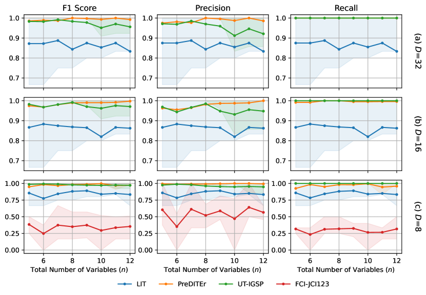
Figure 4: Performance of the algorithms under Setting (1) (Linear Gaussian model under causal sufficiency assumption). Error bars represents the 25% and 75% percentiles of the corresponding metrics. Note that for $D=32$, PreDITEr algorithm (orange line) overlaps with UT-IGSP algorithm (green line) in recall, as both algorithms have 1.0 recall for all $n$.

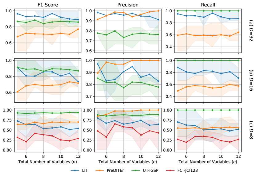
Figure 5: Performance of the algorithms under Setting (2) (Nonlinear model under causal sufficiency assumption). Error bars represents the 25% and 75% percentiles of the corresponding metrics.

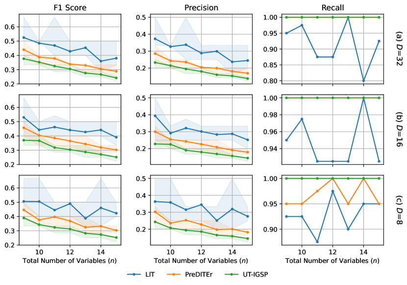
Figure 6: Performance of the algorithms under Setting (3) (Linear Gaussian model in the presence of latent confounders). Error bars represents the 25% and 75% percentiles of the corresponding metrics. Note that PreDITEr algorithm (orange line) overlaps with UT-IGSP algorithm (green line) in recall for $D=32$ and $D=16$. Further, the are no error bars for recall, because the 25% percentile is the same as the 75% percentile (i.e., 1.0) for all three algorithms.

Table 1: Average number of CI tests in LIT algorithm / PDE estimates in PreDITEr algorithm for $D=32$.

Linear, No latent	5	6	7	8	9	10	11	12
LIT	1.00	2.00	1.85	2.85	2.50	2.75	2.45	3.60
PreDITEr	2217.23	2034.00	3309.35	3509.55	5415.05	5566.40	9459.78	9302.95
Nonlinear, No latent	5	6	7	8	9	10	11	12
LIT	16.95	19.85	30.30	36.35	48.10	55.20	70.25	76.45
PreDITEr	2596.38	3095.68	5242.73	4931.48	12152.00	12209.33	22036.25	28876.43
Linear, Latent	9	10	11	12	13	14	15
LIT	1.05	0.80	1.15	1.00	1.30	1.15	1.00
PreDITEr	1460.73	1941.05	2239.43	2275.75	2764.68	3327.98	4076.13

Table 2: Average number of CI tests in LIT algorithm / PDE estimates in PreDITEr algorithm for $D=16$.

Linear, No latent	5	6	7	8	9	10	11	12
LIT	1.10	1.45	1.90	2.25	2.05	2.80	2.85	3.00
PreDITEr	503.68	453.68	848.08	800.65	1221.98	1396.70	2372.85	2135.68
Nonlinear, No latent	5	6	7	8	9	10	11	12
LIT	16.75	20.40	30.70	36.15	48.10	53.20	69.60	78.25
PreDITEr	678.08	779.35	1371.18	1497.60	2910.08	2782.00	6874.65	5987.40
Linear, Latent	9	10	11	12	13	14	15
LIT	1.40	0.75	1.55	0.85	1.25	0.65	1.15
PreDITEr	407.15	442.45	539.78	655.65	611.53	917.40	970.68

References

- Aggarwal et al., (2021) Aggarwal, P., Gupta, A., Mohapatra, P., Nagar, S., Mandal, A., Wang, Q., and Paradkar, A. (2021). Localization of operational faults in cloud applications by mining causal dependencies in logs using golden signals. In Service-Oriented Computing–ICSOC 2020 Workshops: AIOps, CFTIC, STRAPS, AI-PA, AI-IOTS, and Satellite Events, Dubai, United Arab Emirates, December 14–17, 2020, Proceedings, pages 137–149. Springer.
- Brouillard et al., (2020) Brouillard, P., Lachapelle, S., Lacoste, A., Lacoste-Julien, S., and Drouin, A. (2020). Differentiable causal discovery from interventional data. Advances in Neural Information Processing Systems, 33:21865–21877.
- Budhathoki et al., (2022) Budhathoki, K., Minorics, L., Blöbaum, P., and Janzing, D. (2022). Causal structure-based root cause analysis of outliers. In International Conference on Machine Learning, pages 2357–2369. PMLR.
- Darmois, (1953) Darmois, G. (1953). Analyse générale des liaisons stochastiques: etude particulière de l’analyse factorielle linéaire. Revue de l’Institut International de Statistique / Review of the International Statistical Institute, 21(1/2):2–8.
- Eaton and Murphy, (2007) Eaton, D. and Murphy, K. (2007). Exact bayesian structure learning from uncertain interventions. In Artificial intelligence and statistics, pages 107–114. PMLR.
- Geiger and Pearl, (1990) Geiger, D. and Pearl, J. (1990). On the logic of causal models. In Machine Intelligence and Pattern Recognition, volume 9, pages 3–14. Elsevier.
- Ghassami et al., (2017) Ghassami, A., Salehkaleybar, S., Kiyavash, N., and Zhang, K. (2017). Learning causal structures using regression invariance. Advances in Neural Information Processing Systems, 30.
- Hornik et al., (1989) Hornik, K., Stinchcombe, M., and White, H. (1989). Multilayer feedforward networks are universal approximators. Neural networks, 2(5):359–366.
- Hyvarinen and Morioka, (2016) Hyvarinen, A. and Morioka, H. (2016). Unsupervised feature extraction by time-contrastive learning and nonlinear ica. Advances in neural information processing systems, 29.
- Hyvarinen et al., (2019) Hyvarinen, A., Sasaki, H., and Turner, R. (2019). Nonlinear ica using auxiliary variables and generalized contrastive learning. In The 22nd International Conference on Artificial Intelligence and Statistics, pages 859–868. PMLR.
- Hyvärinen et al., (2001) Hyvärinen, A., Karhunen, J., and Oja, E. (2001). Independent Component Analysis. John Wiley & Sons.
- Jaber et al., (2020) Jaber, A., Kocaoglu, M., Shanmugam, K., and Bareinboim, E. (2020). Causal discovery from soft interventions with unknown targets: Characterization and learning. Advances in neural information processing systems, 33:9551–9561.
- Khemakhem et al., (2020) Khemakhem, I., Kingma, D., Monti, R., and Hyvarinen, A. (2020). Variational autoencoders and nonlinear ica: A unifying framework. In International Conference on Artificial Intelligence and Statistics, pages 2207–2217. PMLR.
- Ljung, (1998) Ljung, L. (1998). System identification. Springer.
- Mooij et al., (2020) Mooij, J. M., Magliacane, S., and Claassen, T. (2020). Joint causal inference from multiple contexts. The Journal of Machine Learning Research, 21(1):3919–4026.
- Ness et al., (2017) Ness, R. O., Sachs, K., Mallick, P., and Vitek, O. (2017). A bayesian active learning experimental design for inferring signaling networks. In Research in Computational Molecular Biology: 21st Annual International Conference, RECOMB 2017, Hong Kong, China, May 3-7, 2017, Proceedings 21, pages 134–156. Springer.
- Pearl, (1988) Pearl, J. (1988). Probabilistic reasoning in intelligent systems: networks of plausible inference. Morgan kaufmann.
- Pearl, (2009) Pearl, J. (2009). Causality. Cambridge university press.
- Perry et al., (2022) Perry, R., Von Kügelgen, J., and Schölkopf, B. (2022). Causal discovery in heterogeneous environments under the sparse mechanism shift hypothesis. In Advances in Neural Information Processing Systems.
- Richardson and Spirtes, (2002) Richardson, T. and Spirtes, P. (2002). Ancestral graph markov models. The Annals of Statistics, 30(4):962–1030.
- Sachs et al., (2005) Sachs, K., Perez, O., Pe’er, D., Lauffenburger, D. A., and Nolan, G. P. (2005). Causal protein-signaling networks derived from multiparameter single-cell data. Science, 308(5721):523–529.
- Skitovitch, (1953) Skitovitch, V. P. (1953). On a property of the normal distribution. DAN SSSR, 89:217–219.
- Sorrenson et al., (2020) Sorrenson, P., Rother, C., and Köthe, U. (2020). Disentanglement by nonlinear ica with general incompressible-flow networks (gin). In International Conference on Learning Representations.
- Spirtes et al., (2000) Spirtes, P., Glymour, C. N., Scheines, R., and Heckerman, D. (2000). Causation, prediction, and search. MIT press.
- Squires et al., (2020) Squires, C., Wang, Y., and Uhler, C. (2020). Permutation-based causal structure learning with unknown intervention targets. In Conference on Uncertainty in Artificial Intelligence, pages 1039–1048. PMLR.
- Teshima et al., (2020) Teshima, T., Sato, I., and Sugiyama, M. (2020). Few-shot domain adaptation by causal mechanism transfer. In International Conference on Machine Learning, pages 9458–9469. PMLR.
- Varici et al., (2022) Varici, B., Shanmugam, K., Sattigeri, P., and Tajer, A. (2022). Intervention target estimation in the presence of latent variables. In Uncertainty in Artificial Intelligence, pages 2013–2023. PMLR.
- (28) Yang, Y., Ghassami, A., Nafea, M., Kiyavash, N., Zhang, K., and Shpitser, I. (2022a). Causal discovery in linear latent variable models subject to measurement error. In Advances in Neural Information Processing Systems, volume 35, pages 874–886.
- (29) Yang, Y., Nafea, M. S., Ghassami, A., and Kiyavash, N. (2022b). Causal discovery in linear structural causal models with deterministic relations. In Conference on Causal Learning and Reasoning, pages 944–993. PMLR.