Probabilistic Precipitation Downscaling with Optical Flow-Guided Diffusion

Abstract

In climate science and meteorology, local precipitation predictions are limited by the immense computational costs induced by the high spatial resolution that simulation methods require. A common workaround is statistical downscaling (aka superresolution), where a low-resolution prediction is super-resolved using statistical approaches. While traditional computer vision tasks mainly focus on human perception or mean squared error, applications in weather and climate require capturing the conditional distribution of high-resolution patterns given low-resolution patterns so that reliable ensemble averages can be taken. Our approach relies on extending recent video diffusion models to precipitation superresolution: an optical flow on the high-resolution output induces temporally coherent predictions, whereas a temporally-conditioned diffusion model generates residuals that capture the correct noise characteristics and high-frequency patterns. We test our approach on X-SHiELD, an established large-scale climate simulation dataset, and compare against two state-of-the-art baselines, focusing on CRPS, MSE, precipitation distributions, as well as an illustrative case – the complex terrain of California. Our approach sets a new standard for data-driven precipitation downscaling.

1 Introduction

Patterns of precipitation (rainfall and snowfall) are central to human and natural life on earth. In a rapidly warming climate, reliable simulations of how precipitation patterns may change help human societies adapt to climate change. Such simulations are challenging, because weather systems of many scales in space and time, interacting with complex surface features such as mountains and coastlines, contribute to precipitation trends and extremes [46]. For purposes such as estimating flood hazards, precipitation must be estimated down to spatial resolutions of a few km. Fluid-dynamical models of the global atmosphere are prohibitively expensive to run at such fine scales [52], so the climate adaptation community relies on ‘downscaling’ of coarse-grid simulations to a finer grid (this is the climate science terminology for super-resolution). Traditional downscaling is either ‘dynamical’ (running a fine-grid fluid-dynamical model limited to the region of interest, which requires specialized knowledge and computational resources) or ‘statistical’ (typically restricted to simple univariate methods) [53]. Advances in super-resolution methods developed by the computer vision community are poised to dramatically improve statistical downscaling.

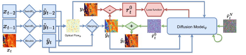
Figure 1: An illustration of the training and inference pipelines of our model. Blue blocks represent operations common to both the training and inference phases. Red blocks signify operations exclusive to training, while green blocks indicate inference-only processes. In summary, our model takes in a current low-resolution frame, and previous context frames. These low-resolution frames are deterministically downscaled and warped via a learned optical flow, followed by modeling of the low-level residual details via diffusion. The model parameters ($\theta=\{\lambda,\phi,\psi\}$) are jointly optimized during training. See Appendix A.1 for further details regarding our model architecture.

Such work is a natural follow-up to recent advancements in deep-learning-based weather and climate prediction methodologies, which have ushered in a new era of data-driven forecasting. These approaches show remarkable performance gains, boasting improvements of orders of magnitude in run time without sacrificing accuracy [35, 24].

Our focus centers on addressing a temporal downscaling problem, wherein the objective is to enhance the resolution of a sequence (“video”) of low-resolution precipitation frames, into a sequence of high-resolution ones. Precipitation has strong temporal continuity on hourly time scales. Hence, even though precipitation data are distinct from natural videos, we adopt ideas from video super-resolution to leverage information from multiple past frames to stochastically downscale the precipitation sequence  [42, 30].

Until recently, endeavors to enhance the resolution of climate states like precipitation have been primarily based on deterministic regression methods that employ convolutions or transformers. However, super-resolution is a one-to-many mapping with a continuum of “correct” answers. Treating such one-to-many problems using supervised learning is therefore prone to visual artifacts since the supervised network tries to predict the average from a multitude of incompatible solutions. Such mode averaging is a known source of blurriness in visual data [25, 63]. While some successful supervised super-resolution methods for images and video have been proposed [8, 20, 62, 6, 19], a natural approach to preventing mode averaging are conditional generative models, due to their ability to capture multi-modal conditional data distributions.

To that end, a line of recent work proposes the use of generative adversarial networks (GANs) for precipitation downscaling. These GAN-based methodologies often encounter challenges, displaying a tendency to converge on a specific mode of the data distribution, occasionally fixating on isolated points in extreme cases. Despite their perceptual appeal, the scientific utility of super-resolution necessitates the accurate modeling of the statistical distribution of high-resolution data given low-resolution input, a facet that GANs typically fall short of capturing.

In this paper, we propose Optical Flow Diffusion (OF-Diff), a diffusion-based generative model for spatiotemporal precipitation downscaling. Our proposed model draws inspiration from and extends related work in neural video compression [1, 59, 60, 40, 31]. In particular, our model uses a learned optical flow to incorporate temporal context, followed by modeling the residual error with a diffusion model, allowing us to add low-level details to the coarse flow-based prediction. Diffusion models are particularly well-suited for precipitation downscaling, as they have been shown to successfully capture high dimensional and multimodal distributions, alleviating a key drawback of GAN-based methods for climate science applications.

This study underscores the capability of conditional diffusion models to meet the specific needs of statistical precipitation downscaling. Specifically, our contributions are:

• We propose a new framework for temporal downscaling based on diffusion models. The model uses a jointly learned optical flow to estimate the motion from previous frames and uses a conditional diffusion model to add low-level texture.

• Our model shows competitive performance against two strong baselines, namely a widely-used image super-resolution model and a state-of-the-art video super-resolution model, in terms of both distributional and perceptual metrics on the X-SHiELD [5, 12] global atmosphere simulation dataset.

Our paper is structured as follows. First, we discuss relevant literature (Sec 4) and its connection to our work. Next, we describe our method (Sec 2), which is then followed by a discussion of our experimental findings (Sec 3).

2 Downscaling via Optical Flow Diffusion

Problem Statement.

We consider sets of paired high-resolution precipitation frame sequences $\mathbf{y}^{0:T}$ and low-resolution precipitation frame sequences $\mathbf{x}^{0:T}$, obtained by coarsening the latter. The superscript represents the frame indices. Each sequence comprises $T+1$ frames (we assume $T$ is fixed for simplicity). Our objective is to train a model to effectively downscale, or super-resolve the given sequence $\mathbf{x}^{0:T}$ with $\mathbf{y}^{0:T}$ serving as the target. Note we use both "downscaling" and "super-resolution" interchangeably.

More formally, let $\mathbf{x}^{t}\in\mathbb{R}^{C\times H\times W}$ and $\mathbf{y}^{t}\in\mathbb{R}^{1\times sH\times sW}$ be the low-resolution and high-resolution frames. Here, $s\in\mathbb{N}$ denotes the downscaling factor, $C$ represents the number of climate states used as input to the model, and $H,W$ indicate the height and width of the low-resolution frames, respectively. For our study, we adopt a downscaling factor of $s=8$ and have $C=13$ total low-resolution channels. In addition to the low-resolution precipitation state, we provide an additional twelve channels of information to the model via concatenation, such as topography, wind velocity, and surface temperature; see Table 1 and Appendix A.2 for details.

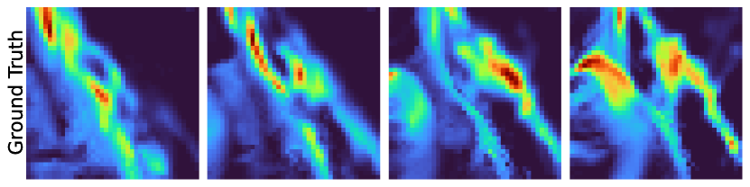
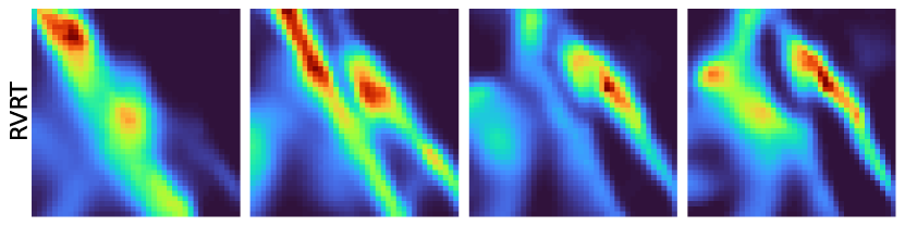
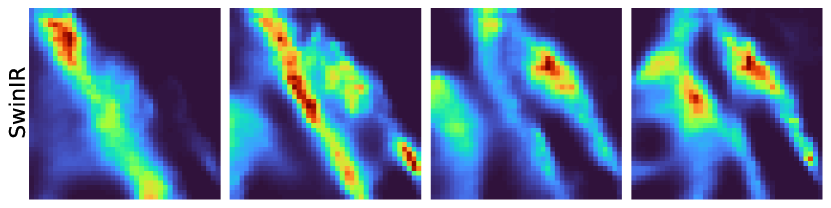
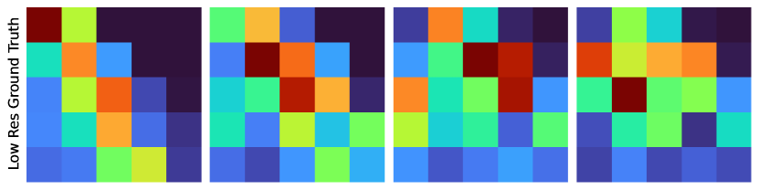
Figure 2: A qualitative comparison between our proposed model and baselines for a specific precipitation event associated with a cold front impinging on the Northern California coast and then the Sierra mountain range. Fig. 4 plots the regional topography. The first row represents the ground truth fine-grid precipitation state sequence, and the last row represents the coarse-grid precipitation that is being downscaled. The other rows correspond to our model and the baseline outputs. The time interval between adjacent frames is 3 hours; the plotted region is $1000\times 1000$ km. Our model more accurately resolves the fine-grid precipitation structure than the considered baselines. See Appendix A.3 for additional samples and qualitative comparisons.

Solution Sketch

We approach the downscaling problem as a conditional generative modeling task. Accordingly, we devise a model with the objective of learning the conditional distribution of high-resolution precipitation frames, taking into account the contextual information provided by the low-resolution precipitation frame sequence.

Our proposed solution, Optical Flow Diffusion (OF-Diff) is sketched in Figure 1 and relies on two modules: a deterministic component based on warping [1] and a stochastic component based on denoising diffusion models [17, 50]. The first module uses motion compensation to deterministically predict a high-resolution frame, which we denote $\tilde{\mathbf{y}}^{t}$. We use several conditioning frames from previous time instants to learn an optical flow, which is used to warp the deterministically-downscaled previous frame $\hat{\mathbf{y}}^{t-1}$ into the current frame. Then, using the motion-compensated high-resolution prediction $\tilde{\mathbf{y}}^{t}$ as a basis, an additive residual $\mathbf{y}^{t}-\tilde{\mathbf{y}}^{t}$ is generated using a conditional diffusion model, adding low-level details, resulting in the predicted high-resolution frame $\check{\mathbf{y}}^{t}$. All modules are trained end-to-end.

In what follows, we first describe our overall probabilistic framework for downscaling. Then, we discuss the deterministic next-frame prediction module and learned optical flow module, followed by the remaining residual prediction module based on diffusion generative modeling. See Appendix A.1 for the details of our model architecture.

2.1 Probabilistic Modeling of Downscaling

Given a sequence of low-resolution frames $\mathbf{x}^{0:T}$ and the corresponding sequence of high-resolution frames $\mathbf{y}^{0:T}$, we seek to learn a parametric approximation $p_{\theta}$ of the underlying conditional distribution $p\left(\mathbf{y}^{0:T}\mid\mathbf{x}^{0:T}\right)$. For computational reasons, we make a second-order Markov assumption, so that each generated high-resolution frame depends only on the current low-resolution frame and two previous low-resolution frames:

$$p_{\theta}\left(\mathbf{y}^{0:T}\mid\mathbf{x}^{0:T}\right)\\ =p_{\theta}(\mathbf{y}^{0}\mid\mathbf{x}^{0})p_{\theta}(\mathbf{y}^{1}\mid\mathbf{x}^{1})\prod_{t=2}^{T}p_{\theta}\left(\mathbf{y}^{t}\mid\mathbf{x}^{t-2:t}\right),$$ (1)

with different treatment of the first two frames (i.e. $t<2$). In what follows, we focus on a single term of this likelihood for $t\geq 2$, i.e. a term of the form $p_{\theta}\left(\mathbf{y}^{t}\mid\mathbf{x}^{t-2:t}\right)$. As discussed in the overview of this section, this likelihood term is modeled using a combination of an optical flow and a residual diffusion model.

As follows, we will discuss how the model parameters $\theta=(\lambda,\phi,\psi)$ decompose an image super-resolution module ($\lambda$), an optical flow ($\phi$), and a diffusion model ($\psi$).

Deterministic Downscaling

First, we construct high-resolution deterministic predictions

$$\hat{\mathbf{y}}^{s}=\nu_{\lambda}(\mathbf{x}^{s})\qquad s=t-2,t-1$$ (2)

for the two low-resolution context frames, where $\nu_{\lambda}$ represents a deterministic downscaling module with parameters $\lambda$. These predictions are made without temporal context. We also generate a smooth high-resolution frame $\overline{\mathbf{y}}^{t}$ from $\mathbf{x}^{t}$ using bicubic interpolation. We choose to use bicubic interpolation for the current frame to help stabilize training and to avoid introducing artifacts from the deterministic downscaling module into the current frame.

We employ a Swin-IR [27], a widely used deterministic downscaler, to super-resolve the two low-resolution context frames. This downscaler is trained end-to-end with the entire model, yielding the estimated outputs $\hat{\mathbf{y}}^{t}$ as illustrated in Figure 1. The Swin-IR module is characterized by the integration of residual Swin Transformer blocks. In Section 3, an ablation study is conducted against a per-frame downscaling baseline employing Swin-IR in isolation. Notably, this baseline cannot match the performance of our comprehensive model.

Here, we note that the first and second frames of a sequence ($t=0,1$) are handled as special cases, where we use $\nu_{\lambda}$ alone in the prediction, i.e. without additional warping and residual modeling.

Motion Estimation via Flow Warping

Next, we use a learned optical flow to warp the high-resolution sequence $(\hat{\mathbf{y}}^{t-2},\hat{\mathbf{y}}^{t-1},\overline{\mathbf{y}}^{t})$ into the final deterministic prediction $\widetilde{\mathbf{y}}^{t}$. More formally, we have that

$$\widetilde{\mathbf{y}}^{t}=w\left(\hat{\mathbf{y}}^{t-1},\mu_{\phi}\left(\overline{\mathbf{y}}^{t},\hat{\mathbf{y}}^{t-1},\hat{\mathbf{y}}^{t-2}\right)\right)$$ (3)

where $w$ is the warping function, and $\mu_{\phi}$ is a network generating the learned warping field with parameters $\phi$.

Our approach draws on analogies between video super-resolution and recent approaches to low-latency neural video decoding [1, 59, 60, 40, 31]. A common approach in predictive coding-based video decompression is to predict (in the best way possible) the next frame in a sequence of video frames well so that the error residuals are sparse and easy to compress [1, 60]. Typically, this is achieved by estimating an optical flow in the video so that the next frame can be predicted using bilinear warping.

In our work, Eq 3 corresponds to a learned optical flow, where a network $\mu_{\phi}$ takes in three sequential deterministically downscaled high-resolution climate states $\left(\overline{\mathbf{y}}^{t},\hat{\mathbf{y}}^{t-1},\hat{\mathbf{y}}^{t-2}\right)$ as context to compute the flow field, which is then used to perform the warping via the bilinear warping function $w$.

Stochastic Residual Modeling via Diffusion

Lastly, our final stochastic high-resolution frame $\check{\mathbf{y}}^{t}$ is generated by sampling a residual $\mathbf{r}_{0}^{t}$ from a conditional diffusion model with parameters $\psi$, i.e.

$$\check{\mathbf{y}}^{t}=\widetilde{\mathbf{y}}^{t}+\mathbf{r}_{0}^{t}.$$ (4)

while not converged do

       Sample $\mathbf{x}^{0:T}$ and $\mathbf{y}^{0:T}$;

       $n\sim\mathcal{U}(0,1,2,..,N)$;

       $L=0$;

       for t = 2 to T do

             $\epsilon\sim\mathcal{N}(\textbf{0},\textbf{I})$;

             $\hat{\mathbf{y}}^{t-2},\hat{\mathbf{y}}^{t-1}=\nu_{\lambda}\left(\mathbf{x}^{t-2}\right),\nu_{\lambda}\left(\mathbf{x}^{t-1}\right)$;

             $\tilde{\mathbf{y}}^{t}=w\left(\hat{\mathbf{y}}^{t-1},\mu_{\phi}\left(\mathbf{x}^{t},\hat{\mathbf{y}}^{t-1},\hat{\mathbf{y}}^{t-2}\right)\right)$;

             $\mathbf{r}^{t}_{0}=\mathbf{y}^{t}-\tilde{\mathbf{y}}^{t}$;

             $\mathbf{v}=\alpha_{n}\epsilon-\sigma_{n}\mathbf{r}^{t}_{0}$;

             $\mathbf{r}_{n}^{t}=\alpha_{n}\mathbf{r}_{0}^{t}+\sigma_{n}\epsilon$;

             $\hat{\mathbf{v}}=M_{\psi}\left(\mathbf{r}_{n}^{t},n,\mathbf{x}^{t},\tilde{\mathbf{y}}^{t}\right)$;

             $L_{diff}=||\mathbf{v}-\hat{\mathbf{v}}||^{2}$;

             $L_{flow}=||\mathbf{y}^{t}-\tilde{\mathbf{y}}^{t}||^{2}$;

             $L_{recon}=||\mathbf{y}^{<t}-\hat{\mathbf{y}}^{<t}||^{2}$;

             $L+=L_{diff}+L_{flow}+L_{swin}$;

       end for

      $(\psi,\phi,\lambda)=(\psi,\phi,\lambda)-\nabla_{\psi,\phi,\lambda}L$;

end while

Algorithm 1 Training OF-Diff

Thus, we seek to model the residuals $\mathbf{r}_{0}^{t}=\mathbf{y}^{t}-\mathbf{\widetilde{y}}^{t}$. In order to do so, we leverage the framework of diffusion models, in particular the DDPM model of Ho et al. [17]. To that end, we introduce a collection of latent variables $\mathbf{r}^{t}=\mathbf{r}_{0:N}^{t}$, where the lower subscripts indicate the denoising diffusion step. We use $N$ to denote the total number of denoising steps. Note that $\mathbf{r}_{0}^{t}$, i.e. the first diffusion step, corresponds to the true residual. We further note that $\mathbf{r}_{0}^{t}$ implicitly depends on the Swin-IR and warping parameters $\lambda$ and $\phi$, and hence we may simultaneously optimize all model parameters $\theta=(\lambda,\phi,\psi)$ within the context of diffusion modeling.

In the forward process of a diffusion model, the latent variable $\mathbf{r}_{n}^{t}$ is created from $\mathbf{r}_{n-1}^{t}$ via additive noise. In the reverse process, which serves to perform generation, a denoising model is trained to predict $\mathbf{r}_{j-1}^{t}$ from $\mathbf{r}_{j}^{t}$. More concretely, the forward process is specified via a collection of Gaussian transition kernels

$$q\left(\mathbf{r}^{t}_{1:N}|\mathbf{r}^{t}_{0}\right) =\prod_{n=1}^{N}q\left(\mathbf{r}^{t}_{n}|\mathbf{r}^{t}_{n-1}\right)$$ (5)

$$q\left(\mathbf{r}^{t}_{n}|\mathbf{r}^{t}_{n-1}\right) ={\cal N}\left(\mathbf{r}^{t}_{n}|\sqrt{1-\beta_{n}}\mathbf{r}^{t}_{n-1},\beta_{n}{\bf I}\right).$$

This process is free of learnable parameters, but requires a hand-chosen variance schedule ${\beta_{n}\in(0,1)}$ for ${n\in\{1,\ldots,N\}}$ [50, 17]. The reverse process, which is a variational approximation of the true time-reversal of the forward process, is defined similarly for $t\geq 2$ via

$$p_{\psi}\left(\mathbf{r}_{0:N}^{t}|\overline{\mathbf{y}}^{t},\widetilde{\mathbf{y}}^{t}\right)=p\left(\mathbf{r}_{N}^{t}\right)\prod_{n=1}^{N}p_{\psi}\left(\mathbf{r}_{n-1}^{t}|\mathbf{r}_{n}^{t},\mathbf{z}^{t}\right)$$ (6)

where $\mathbf{z}^{t}=(\overline{\mathbf{y}}^{t},\widetilde{\mathbf{y}}^{t},\hat{\mathbf{y}}^{t-1},\hat{\mathbf{y}}^{t-2})$ is a tuple of information used to condition the diffusion model at frame $t$. Here, we note that the diffusion model directly accesses $\overline{\mathbf{y}}^{t}$ and $\widetilde{\mathbf{y}}^{t}$, but is only implicitly conditioned on $\hat{\mathbf{y}}^{t-1},\hat{\mathbf{y}}^{t-2}$ via concatenation of feature maps from the flow module.

As is standard in diffusion models [17], we parameterize the reverse process via a Gaussian distribution whose mean is determined by a neural network $M_{\psi}$, i.e.

$$p_{\psi}\left(\mathbf{r}_{n-1}^{t}|\mathbf{r}_{n}^{t},\mathbf{z}^{t}\right)={\cal N}\left(\mathbf{r}_{n-1}^{t}|M_{\psi}\left(\mathbf{r}_{n}^{t},n,\mathbf{z}^{t}\right),\gamma{\bf I}\right),$$ (7)

where $M_{\psi}$ is a denoising network. Here, the variance $\gamma$ is a hyperparameter.

Get an equally spaced increasing sub-sequence $\tau$ of $\left[1,\ldots,N\right]$ of length $S\ll N$, i.e., $\{\tau_{1},\ldots,\tau_{S}\}$;

for t = 2 to T do

       $\hat{\mathbf{y}}^{t-2},\hat{\mathbf{y}}^{t-1}=\nu_{\lambda}\left(\mathbf{x}^{t-2}\right),\nu_{\lambda}\left(\mathbf{x}^{t-1}\right)$;

       $\tilde{\mathbf{y}}^{t}=w\left(\hat{\mathbf{y}}^{t-1},\mu_{\phi}\left(\overline{\mathbf{y}}^{t},\hat{\mathbf{y}}^{t-1},\hat{\mathbf{y}}^{t-2}\right)\right)$;

       $\mathbf{r}_{S}^{t}\sim\mathcal{N}(\textbf{0},\textbf{I})$;

       for n in reversed($\tau$) do

             $\hat{\mathbf{v}}=M_{\psi}\left(\mathbf{r}_{n}^{t},n,\mathbf{x}^{t},\tilde{\mathbf{y}}^{t}\right)$;

             $\hat{\mathbf{r}}=\alpha_{n}\mathbf{r}_{n}^{t}-\sigma_{n}\hat{\mathbf{v}}$;

             $\hat{\epsilon}=\frac{\sigma_{n}}{\alpha_{n}}\left(\mathbf{r}_{n}^{t}-\hat{\mathbf{r}}\right)$;

             $\mathbf{r}^{t}_{n-1}=\alpha_{n-1}\hat{\mathbf{r}}+\sigma_{n-1}\hat{\epsilon}$;

       end for

      $\check{\mathbf{y}}^{t}=\tilde{\mathbf{y}}^{t}+\mathbf{r}^{t}_{0}$;

end for

Algorithm 2 Downscaling with OF-Diff

Loss Function

To train our model, we use the angular parametrization suggested by Salimans and Ho [47]. More concretely, this results in the diffusion loss of the form

$$L_{\text{diff}}(\lambda,\psi,\phi)=\mathbb{E}_{\mathbf{x},\mathbf{y},n,\epsilon}\sum_{t=0}^{T}\|\mathbf{v}-M_{\psi}\left(\mathbf{r}_{n}^{t},n,\mathbf{z}^{t}\right)\|^{2}$$ (8)

where $\epsilon\sim\mathcal{N}(0,I)$ is standard Gaussian noise, and the scalars $\alpha_{n}^{2}=\prod_{i=1}^{n}(1-\beta_{i})$ and $\sigma_{n}^{2}=1-\alpha_{n}^{2}$ are used to define $\mathbf{v}\equiv\alpha_{n}\epsilon-\sigma_{n}\mathbf{r}_{0}^{t}$.

We add two additional loss terms to steer the super-resolution approach into a desired behavior:

$$L_{\text{flow}}(\lambda,\phi) =\mathbb{E}_{\mathbf{x},\mathbf{y}}\sum_{t=0}^{T}\|\mathbf{y}^{t}-\mathbf{\tilde{y}}^{t}\|^{2},$$ (9)

$$L_{\text{swin}}(\lambda) =\mathbb{E}_{\mathbf{x},\mathbf{y}}\sum_{t=0}^{T}\|\mathbf{y}^{t}-\mathbf{\hat{y}}^{t}\|^{2}.$$

The first term, $L_{flow}$, regresses the output of the flow module to match the ground truth frame, making sure that the flow module performs warping and learns an accurate flow map. A second term, $L_{swin}$, is an additional frame-wise $L2$ penalty regressing the Swin-IR output to the ground truth frame. The final learning objective is the sum of these three loss terms: $L=L_{diff}+L_{flow}+L_{recon}$.

In order to parallelize the training procedure across multiple time steps, we employ teacher forcing [22]. Algorithms 1 and 2 concisely demonstrates the training and sampling strategy under the angular parametrization. Note that we use the DDIM sampling [49] in order to generate frame residuals with fewer diffusion steps.

3 Experiments

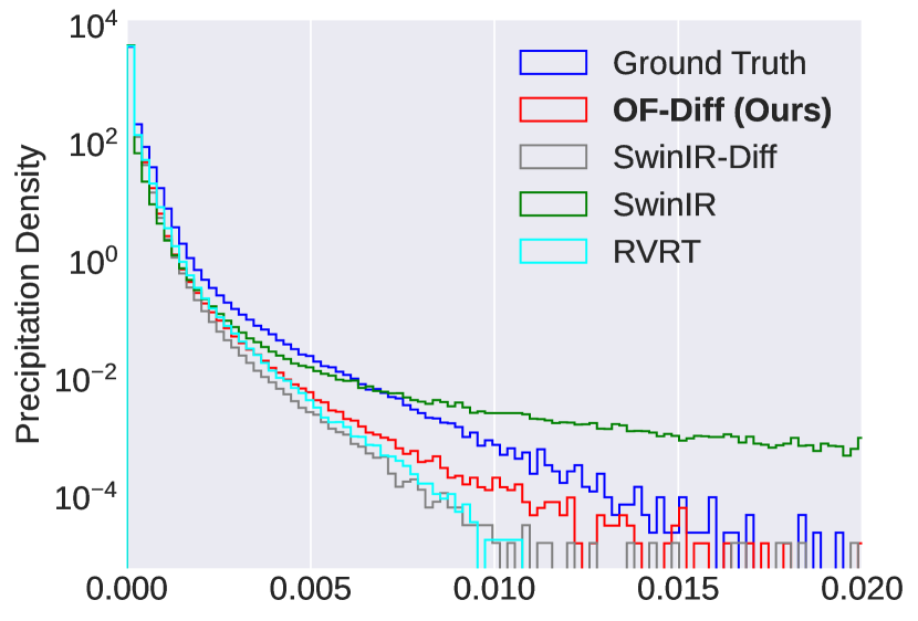
Figure 3: Distributions of the fine-grid three-hourly average precipitation, including all gridpoints around the globe, for each model. The SwinIR baseline overestimates large precipitation events, whereas the SwinIR-Diff and RVRT baselines underestimate precipitation. Our model more closely aligns with the fine-grid ground truth than the other models.

We conduct a comprehensive evaluation of our proposed method, Optical Flow conditioned Diffusion (OF-Diff), against two contemporary state-of-the-art baselines. The first baseline is an image super-resolution model based on the Swin Vision Transformer (SwinIR)[27], while the second baseline is a video super-resolution model grounded in a recurrent and parallelized vision transformer architecture (RVRT) [29]. The latter incorporates guided deformable attention for clip alignment, enhancing its temporal modeling capabilities.

To further scrutinize the efficacy of our proposed method, we perform an ablation study in two distinct configurations. In the first ablation (Swin-IR-Diff), we remove the optical flow module, rendering the ablated model akin to a residual version of Saharia et al.’s image super-resolution method [44], with a Swin-IR backbone. The second ablation (OF-Diff-Single) involves removing the additional input channels (i.e. only providing the model with the low-resolution precipitation sequence) to assess their impact on performance metrics, providing valuable insights into the influence of these supplementary inputs on the model’s overall performance.

3.1 Dataset

Our training and testing data derives from a 11-years-long simulation with a global storm-resolving atmosphere model, X-SHiELD, with an ultra-fine 3 km horizontal grid spacing ideally suited for representing precipitation patterns from global to local scales. The first ten years are used for training, and the last year is used for testing. X-SHiELD [13, 5], developed at the National Oceanic and Atmospheric Administration’s (NOAA) Geophysical Fluid Dynamics Laboratory (GFDL), is an experimental version of NOAA’s operational global weather forecast model.

Three-hourly average data were saved from this entire simulation, which was a 25 km horizontal ‘fine grid’. For this project, we further 8-fold coarsened the selected fields to a 200 km horizontal ‘coarse grid’ to create paired data ($x_{t},y_{t}$), where $x_{t}$ is the coarse-grid global state, and $y_{t}$ is the corresponding fine-grid global state. Our goal is to apply video downscaling / super-resolution to the coarse-grid precipitation field to obtain temporally smooth fine-grid precipitation estimates that are statistically similar to the true data. This approach is attractive because many fine-grid precipitation features, such as cold fronts and tropical cyclones, are poorly resolved on the coarse grid but are temporally coherent across periods much longer than 3 hours. We use 15 coarse-grid input fields, including precipitation and topography, and vector wind at various levels. See Table 1 for the list of included atmospheric variables.

Table 1: Variables in X-SHiELD dataset.

Short Name	Long Name	Units
CPRATsfc	Surface convective precip. rate	kg/m2/s
DSWRFtoa	Top of atmos. down shortwave flux	W/m2
TMPsfc	Surface temperature	K
UGRD10m	10-meter vertical winds	m/s
VGRD10m	10-meter horizontal	m/s
ps	Surface pressure	Pa
u700	700-mb vertical winds	m/s
v700	700-mb horizontal winds	m/s
liq_wat	Vert. integral of cloud water mix ratio	kg/kg kg/m2
sphum	Vert. integral of specific humidity	kg/kg kg/m2
zsurf	Topography	–

The application presented here is a pilot for broader applications of our methodology. Fine-grid simulations are much more computationally expensive than coarse-grid simulations (an 8-fold reduction in grid spacing requires almost 1000x more computation), so a coarse-grid simulation with super-resolved details in desired regions could be highly cost-effective for many weather and climate applications.

X-SHiELD uses a cubed-sphere grid, in which the surface of the globe is divided into six tiles, each of which is covered by an $N\times N$ array of points. Thus our data fields reflect this structure with $N=48$ for the 200 km coarse grid and $N=384$ for the 25 km fine grid.

During the training phase, our VSR model randomly selects data at each time from one of the six tiles. This strategy ensures that the model learns from the diverse spatial contexts and weather regimes that produce precipitation in different parts of the world. Post-training, for localized analysis, we selectively sample super-resolved precipitation channels from regions with complex terrain, such as California, which can systematically pattern the precipitation on fine scales, to see how well the super-resolution can learn the time-mean spatial patterns (e.g. precipitation enhancement on the windward side of mountain ranges and lee rain shadows) in the fine-grid reference data.

3.2 Training and Testing Details

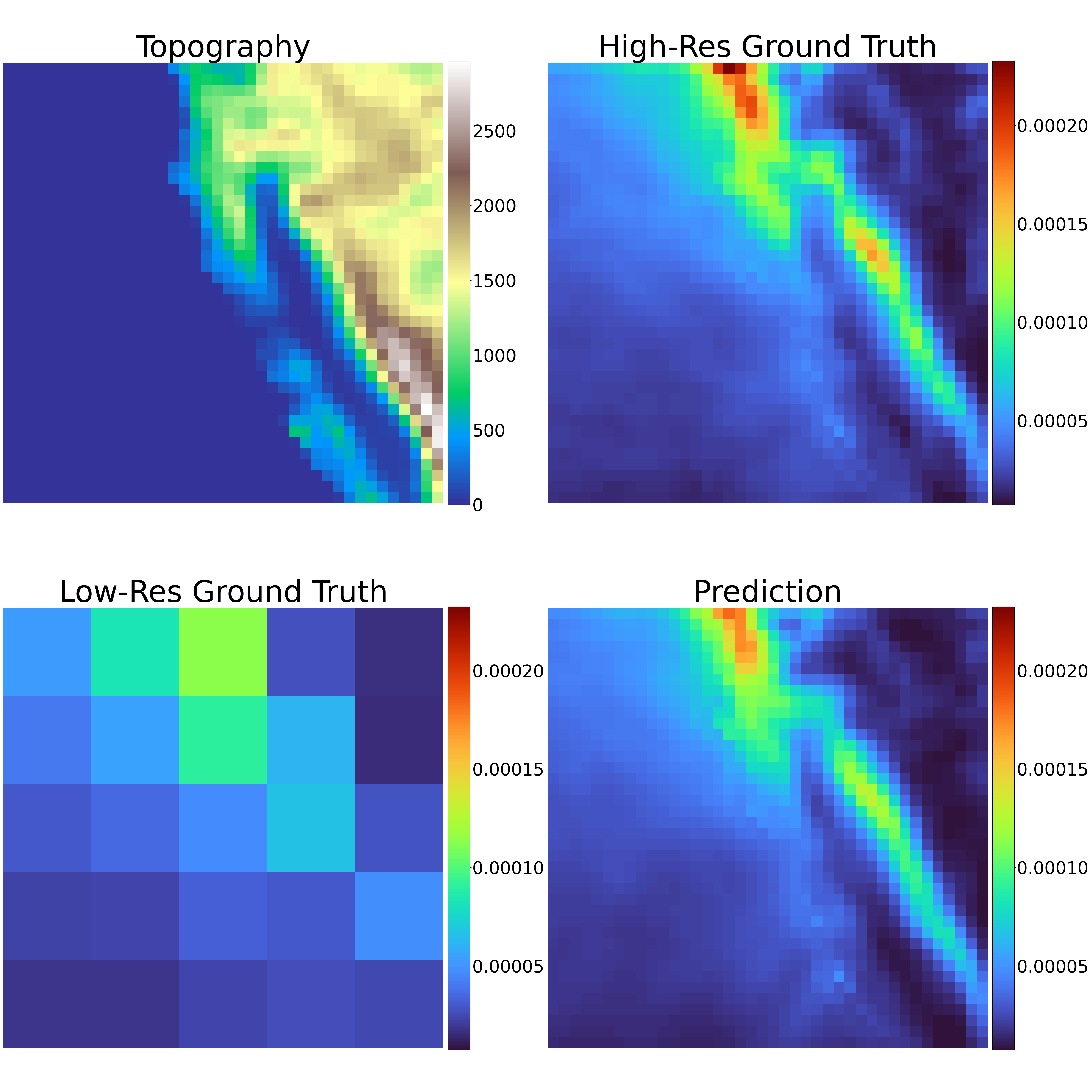
Figure 4: Precipitation over the same region as Fig. 2, averaged across a year, for our OF-Diff model and the ground-truth. The topography of the region is shown in the top-left. Annually-averaged precipitation is an important indicator of water availability in a region. OF-Diff successfully captures many details of the precipitation that are tied to local topography and are too fine to be resolved the coarse-grid data.

We address the task of downscaling a sequence of precipitation climate states with a scale factor of 8 applied to X-SHiELD output. The batch size is set to 1, and precipitation values are logarithmically transformed before normalization to a standardized range of $[-1,1]$.

The optimization of our model is facilitated by the Adam optimizer [21], initializing with a learning rate of $1\times 10^{-4}$. We employ cosine annealing with decay until $5\times 10^{-7}$ during training, executed on an NVidia RTX A6000 GPU. The diffusion model is trained using v-parametrization, with a fixed diffusion depth ($N=1400$). Random tiles extracted from the cube-sphere representation of Earth, with dimensions 384 in high resolution and 48 in low resolution, are utilized during training. The training process spans a million stochastic gradient steps, requiring approximately 7 days on a single node.

During testing, we employ DDIM sampling with 20 steps on an Exponential Moving Average (EMA) variant of our model, with a decay rate set to 0.995. Testing is conducted on the full frame size. Three distinct losses are jointly optimized: the first pertains to the diffusion loss for v-parametrization, the second enforces a flow-warping loss on the output of the flow module, and the final loss imposes a restoration criterion over the Swin-IR module.

3.3 Baseline Models

The recent vision transformer baseline, Recurrent Video Restoration Transformer (RVRT) [29] adopts parallel frame prediction coupled with long-range temporal dependency modeling. Notably, it incorporates guided deformable attention for effective clip alignment, enhancing its temporal modeling capabilities.

In contrast, Swin-IR [27] is an image super-resolution model that harnesses Swin Transformer blocks to reconstruct missing details. Unlike RVRT, Swin-IR focuses on the high-resolution image reconstruction domain.

For the diffusion baseline, we draw inspiration from a modification of SR3 [44]. SR3 is recognized as a classifier-free, conditionally guided diffusion model applied to image super-resolution. In our adaptation (Swin-IR-Diff), the model predicts a residual component; the deterministic base prediction is generated using a Swin-IR model.

3.4 Evaluation Metrics

For this unconventional application, we evaluate our model differently than for standard vision tasks. In addition to Mean Square Error (MSE), our assessment incorporates the Continuous Ranked Probability Score (CRPS), a forecasting metric and recognized scoring rule traditionally associated with time-series data. CRPS evaluates the model’s performance by assessing the coverage of the generated sequence, quantifying calibration of the model’s stochasticity.

Three-hourly precipitation has a distinctive, approximately exponential temporal distribution. For practical applications involving planning human infrastructure to withstand extreme flooding and droughts, it is important to ensure that the application of downscaling does not induce significant alterations in the frequency distribution of precipitation rates. Consequently, we present two distribution-oriented metrics. The first metric employs the Earth Mover Distance to quantify the global agreement between the target and predicted distribution. A second metric assesses model skill in predicting rare extreme precipitation events. It is calculated as the error in the 99.999th percentile across all fine grid points and times of three-hourly precipitation (PE).

Table 2: Quantitative comparison between our OF-Diff method and the various competitive baselines. EMD represents the Earth-Mover Distance, and PE denotes the 99.999th percentile error. Overall, our proposed method (OF-Diff) outperforms the baselines across all metrics, often by orders of magnitude. The exclusion of additional side information (OF-Diff-single) or optical flow component (Swin-IR-Diff) appreciably degrades performance. The models which are deterministic (RVRT and Swin-IR) are outperformed by our diffusion-based methods except on MSE.

	CRPS	MSE	EMD	PE
	$(10^{-5})$	$(10^{-6})$	$(10^{-6})$	$(10^{-3})$
OF-Diff (ours)	$\mathbf{1.67}$	$0.006$	$\mathbf{5.68}$	$\mathbf{1.71}$
OF-Diff-single (ours)	$1.87$	$0.008$	$6.83$	$2.35$
Swin-IR-Diff (ablation)	$1.88$	$0.019$	$7.50$	$2.71$
RVRT [29]	$1.88$	$\mathbf{0.005}$	$6.84$	$2.25$
Swin-IR [27]	$3.19$	$2.54$	$17.62$	$16.00$

3.5 Qualitative and Quantitative Analysis

Table 2 presents a comprehensive quantitative evaluation comparing our method with state-of-the-art baselines and ablations. In terms of model nomenclature, OF-Diff is the model that we propose, with OF-Diff-Single being a single-state variant (that only uses precipitation as opposed to OF-Diff, which also uses other states like wind velocity and topography). Finally, Swin-IR-Diff (as explained in 3.3 is an ablation for the optical flow module (details in Appendix A.2). OF-Diff performs best on three of our four metrics. The incorporation of multiple atmospheric inputs yields additional improvement in the metrics compared to using precipitation alone (OF-diff-single). Our state-of-the-art video super-resolution baseline, RVRT, performs better on MSE, but worse on CRPS. Typically, in climate and weather forecasting, stochastic metrics are more meaningful since they account for the diverse outcomes that are not measured by MSE. The swin-IR model emerges as the least effective among the considered models.

Figure 3 compares the ground truth PDF of the three-hourly fine grid precipitation rate (sampling all grid columns across the goal and all 3-hourly samples across the simulated year) with our method and the ablations. Our method outperforms the others, with Swin-IR predicting too much extreme precipitation, while RVRT and our ablated model Swin-IR-Diff significantly underestimate extreme precipitation. OF-Diff also has the smallest earth-mover distance from the ground truth PDF, and the smallest 99.999th percentile error, which assesses the degree of disagreement for the most extreme events.

Figure 2 depicts the performance of our model compared to other baselines on an example of a precipitation feature interacting with mountainous terrain, using a three-hourly succession of plots. A cold front (linear feature in the left-most column of plots) impinges on northern California, producing enhanced precipitation first over the coastal foothills and then over the northwest-southeast ridge of the Sierra mountain range in the lower right corner of the images. Our model generates high-quality results which preserve most patterns with a high degree of similarity. RVRT produces slightly more diffuse precipitation features, while Swin-IR produces slightly more pixelated precipitation features. All super-resolution methods add useful detail to the coarse-grid precipitation in the lowest row.

Lastly, Figure 4 shows annual-averaged precipitation from the patch from Figure 2. Climate is the average of weather, and for climate purposes, an accurate depiction of the fine-grid structure of time-mean precipitation is important for assessing long-term water availability. Our method (which includes fine-grid topography as a training input) is remarkably successful in replicating the ground truth, including the strength and narrow spatial structure of the bands of high precipitation along the Northern California coastal mountains and the Sierras. These features are not resolved by the coarse-grid inputs to the super-resolution. See Appendix A.3 for additional samples and comparisons.

4 Related Work

Diffusion Models

Diffusion models [48, 17, 55, 50, 51] are a powerful class of deep generative models which generate data via an iterative denoising process. These models have been applied across a wide range of domains, including images [7], audio [23] and point clouds [32]. Most closely related to our work are diffusion models for video. Yang et al. [61] propose a video generative model which generates deterministic next-frame predictions autoregressively, and a diffusion model is used to generate frame residuals for higher quality generations. Harvey et al. [15] use diffusion models to generate videos of several minutes in length, but only on restricted domains.

Image Super-Resolution

Single image super-resolution is a challenging and important task in computer vision [57]. While there exist many classical approaches to this problem [3, 9], in recent years deep learning based methods have become the dominant paradigm [57]. Such approaches treat it as a supervised learning problem, where models are trained to minimize the error between generated and ground-truth images [62, 6, 27]. On the other hand, generative approaches [34, 44, 2] model the data distribution itself, often leading to higher quality outputs.

Cascaded diffusion models for images [38, 43] and SR3 [44] propose a model for single image super-resolution and can’t typically leverage the temporal context.

Video Super-Resolution

There are many approaches for video super-resolution not based on diffusion models [4, 10, 18]. We refer to Liu et al. [30] for a more comprehensive overview of this literature. The recent VRT model [28] is a transformer-based architecture for video super-resolution with an outperforming recurrent variant RVRT [29] that focusses on parallel decoding and guided clip alignment. We note that these recent state-of-the-art approaches are all supervised, i.e. the loss function used during training directly measures the error between the ground-truth images and the images generated by the model. In contrast, our approach is generative, allowing us to directly model the (conditional) data distribution, thus preventing mode averaging.

Data-driven weather and climate modeling

Advancements in climate data processing and downscaling have prominently featured the application of CNNs. Teufel et al. [54] draw inspiration from FRVSR [45], adopting an iterative approach that utilizes the high-resolution frame estimated in the previous step as input for subsequent iterations. Yang et al. [58] employed Fourier neural operators for versatile downscaling. Harder et al. [12] generate physically consistent downscaled climate states by employing a softmax layer to enforce conservation laws.

Concurrent work [33] employs diffusion models for the downscaling of climate states at each time point. GANs have also been used extensively in downscaling and precipitation prediction, as reviewed in recent literature [26, 36, 14, 39, 11, 56].

5 Conclusion

We propose an autoregressive video super-resolution method for probabilistic precipitation downscaling. Our model, OF-Diff, operates by deterministically super-resolving and warping the temporal context of a given frame, followed by stochastically modeling the low-level residual details via diffusion.

We demonstrate empirically that our model can successfully resolve fine-grid structures from coarse-grid information in a temporally coherent manner. In addition, our method outperforms several competitive baselines on a range of quantitative metrics. Our work is an important step towards designing effective data-driven weather forecasting methods which can augment the abilities of numerical simulations, with potential applications to low-latency online weather forecasting.

Potential negative impacts

Despite the intended positive impacts of making the weather more predictable, our approach could potentially be misleading if adapted blindly to a dataset with a relative distribution shift, causing the model performance to degrade. Such an approach could cause the potential underestimation of extreme weather risks such as droughts or extreme rain events. To mitigate these risks, the model should be rigorously tested and re-trained on the data sets of interest.

Acknowledgements

We thank Kushagra Pandey for valuable feedback. Prakhar Srivastava was supported by the Allen Institute for AI summer internship for much of this work. Stephan Mandt acknowledges support from the National Science Foundation (NSF) under an NSF CAREER Award, award numbers 2003237 and 2007719, by the Department of Energy under grant DE-SC0022331, by the IARPA WRIVA program, and by gifts from Qualcomm and Disney. Gavin Kerrigan is supported in part by the HPI Research Center in Machine Learning and Data Science at UC Irvine.

A.1 Model Architecture

Our architecture is a flow-conditioned extension of the DDPM [17] and SR3 [44] models. As discussed in Section 2, Figure 5 outlines the architecture of the proposed denoising and flow-predicting networks. Furthermore, Figure 6 outlines the detail of each box. Before elaborating on the details, we define the naming convention for the parameter choices that we adopt in this section:

• ChannelDim: channel dimension of all the components in the first downsampling layer of the U-Net [41] style structure used in our approach.

• ChannelMultipliers: channel dimension multipliers for subsequent downsampling layers (including the first layer) in both the flow-prediction and denoising modules. The upsampling layer multipliers follow the reverse sequence.

• ResBlock: leverages a standard implementation of ResBlock [16], i.e., two blocks each with a weight-standardised convolution [37] of $3\times 3$ kernel, Group Normalization over groups of 8 and SiLU activation, followed by a channel-adjusting $1\times 1$ convolution.

• LinearAttention: leverages a standard implementation of linear attention with 4 attention heads, each 32 dimensional.

• MLP: conditioning on the denoising step $n$ is achieved through this block which uses 32-dimensional random Fourier features, followed a linear layer, GELU activation and another linear layer to transform the noise step to a higher dimension.

• Cov/TransCov: these are convolutional ($3\times 3$ kernel) downsampling and upsampling blocks that change the spatial size by a factor of 2.

Fig 5 shows how the U-Net from both the denoising and flow-prediction networks interact with each other. The top U-Net depicts the denoising network whereas the bottom U-Net depicts the flow-prediction network.

The denoising network is conditioned in three ways. First, the network is conditioned on the low-resolution frame $\mathbf{x}^{t}$ by upsampling the low-resolution $48\times 48$ tile to $384\times 384$ using bicubic interpolation (which is $\mathbf{\bar{y}}^{t}$) and concatenating it with both $\mathbf{r}^{t}_{n}$ (noisy residual) and $\mathbf{\tilde{y}}^{t}$ (warped output) along the channel dimension. Second, the network is also conditioned on the feature maps generated by the flow-prediction network, i.e., $\mu_{\phi}\left(\overline{\mathbf{y}}^{t},\hat{\mathbf{y}}^{t-1},\hat{\mathbf{y}}^{t-2}\right)$ (see Eq 3) as shown via the green arrows connecting the downsampling units of both the networks. As detailed in the figure, ResBlocks (both the first one and the next with LinearAttention) from downsampling layers of the flow-prediction network yield a feature map that gets concatenated along the inputs of both ResBlocks of the downsampling layer of the denoising network. Finally, each downsampling and upsampling unit of the network gets conditioned on the denoising step $n$ as shown via the black arrows. This conditional embedding for the step is generated through MLP. As shown in the Figure, this embedding is received by both ResBlocks of downsampling and upsampling units. The information flows from the noisy residual through the network, as shown via blue arrows to predict the angular parameter $\mathbf{v}$. Both U-Nets have skip connections (shown via red arrows) between both ResBlocks of downsampling and upsampling layers.

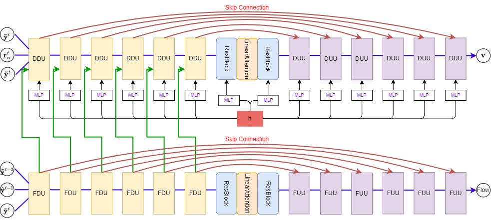
Figure 5: The figure depicts the overall model architecture where the top U-Net performs diffusion on the residual, conditioned both on the noise step $n$ and the context of the bottom U-Net which predicts the flow-field required for motion-compensated prediction. Details of each block are shown in Figure 6.

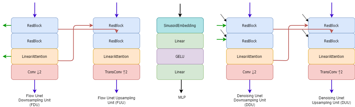
Figure 6: The details of the components of the modules depicted in Figure 5; the colored arrows in the module components correspond to the arrows with the same color in Figure 5.

TileSize	ChannelDim	ChannelMultipliers
$384\times 384$	64	1,1,2,2,3,4

Table 3: X-SHiELD uses a cubed-sphere grid, in which the surface of the globe is divided into six tiles. A single high-resolution tile covers 25km and is $384\times 384$. Our UNet Encoder and Decoder has 6 layers with a base channel dimension of 64 and multipliers as stated above.

A.2 On Swin-IR-Diff and Multiple Channels

Here, we discuss SwinIR-Diff, which expands on one of our robust baselines and also serves as an ablation for the optical-flow module. Section 3.3 provides a concise overview of Swin-IR-Diff. Shown as a sketch in Figure 7, this model eliminates the flow module, opting to downscale each precipitation state individually, akin to an image super-resolution model. Resembling SR3 in its foundation of a conditional diffusion model, Swin-IR-Diff adopts a residual pipeline. It involves a deterministic prediction corrected by a residual generated from the conditional diffusion model, with the Swin-IR model serving as the deterministic downscaler in this context.

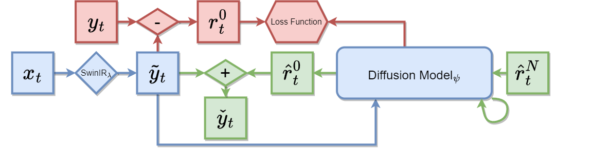
Figure 7: An illustration of the training and inference pipelines of Swin-IR-Diff. Similar to Figure 1, blue blocks represent operations common to both training and inference phases. Red blocks signify operations exclusive to training, while green blocks indicate inference-only processes. However, in a major contrast to Figure 1, the optical flow module is missing. In summary, this model takes in a current low-resolution frame which is deterministically downscaled via Swin-IR, followed by modeling of the low-level residual details via conditional diffusion. The model details remain similar to what is described in A.1 with the absence of flow-conditioning in the diffusion model.

We conducted another ablation, focusing on the incorporation of additional climate states as input to our precipitation downscaling model OF-Diff. The rationale for including these states is drawn from the insights of Harris et al. [14], who justified a similar selection for the task of precipitation forecast based on domain science. While Table 1 provides detailed information on the various states employed, the utility of these states is closely examined in Table 2, with specific attention to OF-Diff (multiple input states) and OF-Diff-single (only precipitation state as input). Clearly, the introduction of additional channels yields a notable improvement in performance.

A.3 Additional Samples

In addition to illustrating precipitation downscaling in the Sierras and Central California, we present our model’s output for another unique region—the Himalayas. Figure 10 mirrors Figure 2, displaying outputs from different models. Additionally, Figure 8 compares the annual precipitation time average for the Himalayas.

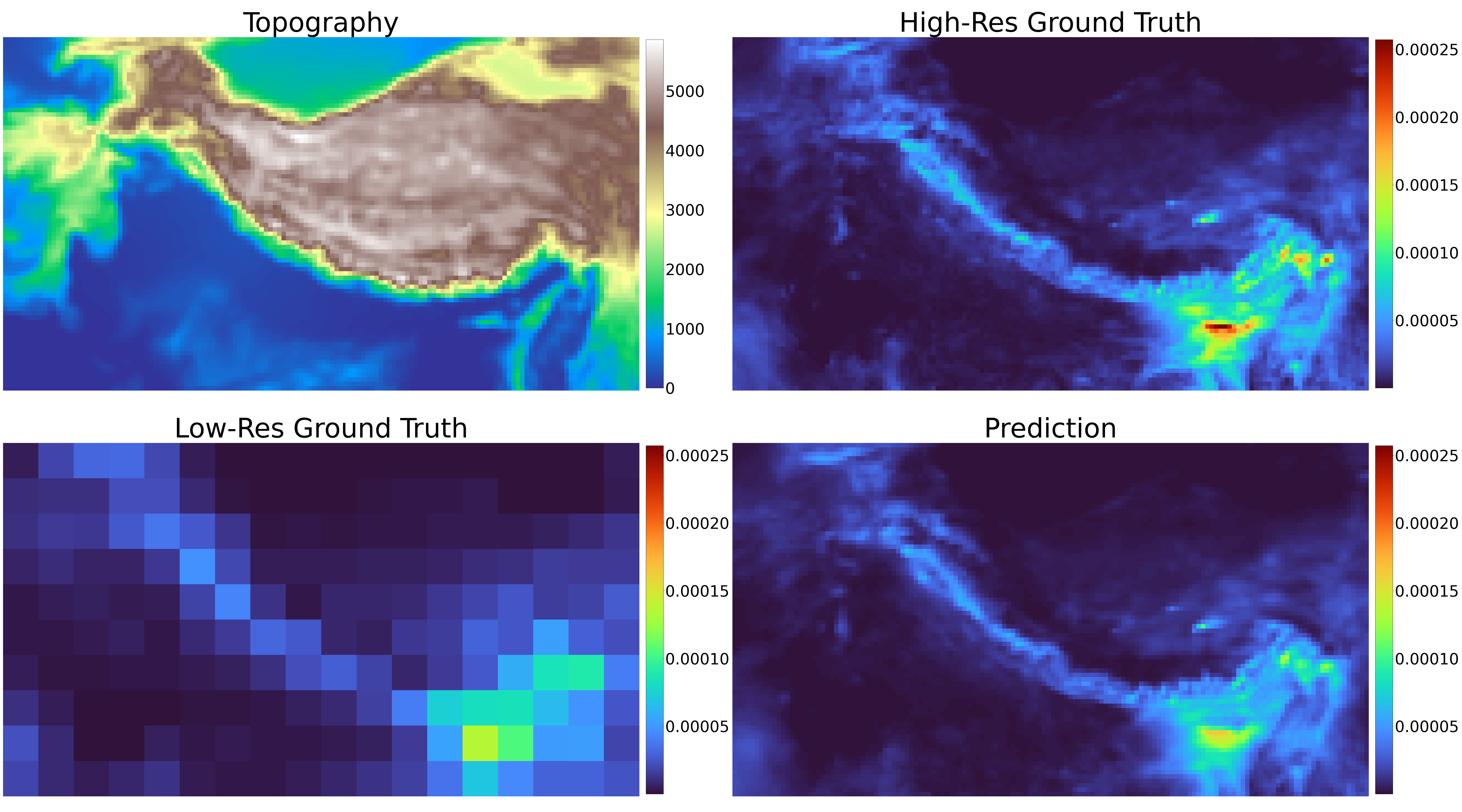
Figure 8: Precipitation over the same region as Fig. 10, averaged across a year, for our OF-Diff model and the ground-truth. The to- pography of the region is shown in the top-left.

A.3.1 Spectra

In Figure 9, we plot the squared-magnitude of the complex-valued FFT applied to the images in our evaluation set. We average these square-magnitudes over the evaluation set, and plot the resulting image on a log-scale. Overall, we see that the samples from OF-Diff closely match the ground-truth high resolution spectrum. The baselines Swin-IR-Diff and RVRT demonstrate a spectrum which decays too rapidly, placing too little energy in the high-frequency components. This indicates that these baselines are overly smooth compared to the ground-truth. For the SwinIR baseline, we observed outliers of large magnitudes in the generated precipitation maps, which we hypothesize leads to the observed checkerboard pattern seen in the spectrum.

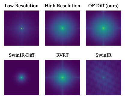
Figure 9: Both the Swin-IR-Diff ablation and RVRT baseline show a spectra which decays too rapidly, i.e. placing too little energy on the high-frequency components. The SwinIR baseline exhibits checkerboard pattern in the spectra. Overall, the spectra of samples from our method most closely match the ground-truth spectra.

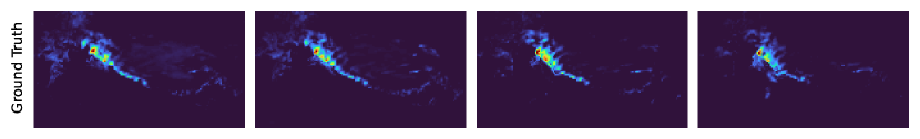
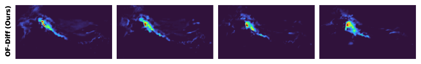
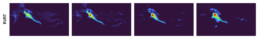
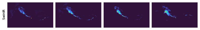
Figure 10: Another qualitative comparison between our proposed model and baselines for a specific precipitation event in the Himalayan mountain range. Fig. 8 plots the regional topography. Similar to Fig. 2 the first row represents the ground truth fine-grid precipitation state sequence, and the last row represents the coarse-grid precipitation that is being downscaled. All other rows correspond to our model and the baseline outputs. The time interval between adjacent frames is 3 hours; the plotted region is $2000\times 3600$ km.

References

- Agustsson et al. [2020] Eirikur Agustsson, David Minnen, Nick Johnston, Johannes Balle, Sung Jin Hwang, and George Toderici. Scale-space flow for end-to-end optimized video compression. In Proceedings of the IEEE/CVF Conference on Computer Vision and Pattern Recognition, pages 8503–8512, 2020.
- Andrei et al. [2021] Silviu S Andrei, Nataliya Shapovalova, and Walterio Mayol-Cuevas. SUPERVEGAN: Super resolution video enhancement GAN for perceptually improving low bitrate streams. IEEE Access, 9:91160–91174, 2021.
- Bascle et al. [1996] Benedicte Bascle, Andrew Blake, and Andrew Zisserman. Motion deblurring and super-resolution from an image sequence. In Computer Vision—ECCV’96: 4th European Conference on Computer Vision Cambridge, UK, April 15–18, 1996 Proceedings Volume II 4, pages 571–582. Springer, 1996.
- Chan et al. [2021] Kelvin CK Chan, Xintao Wang, Ke Yu, Chao Dong, and Chen Change Loy. Basicvsr: The search for essential components in video super-resolution and beyond. In Proceedings of the IEEE/CVF Conference on Computer Vision and Pattern Recognition, pages 4947–4956, 2021.
- Cheng et al. [2022] Kai-Yuan Cheng, Lucas Harris, Christopher Bretherton, Timothy M Merlis, Maximilien Bolot, Linjiong Zhou, Alex Kaltenbaugh, Spencer Clark, and Stephan Fueglistaler. Impact of warmer sea surface temperature on the global pattern of intense convection: insights from a global storm resolving model. Geophysical Research Letters, 49(16):e2022GL099796, 2022.
- Dai et al. [2019] Tao Dai, Jianrui Cai, Yongbing Zhang, Shu-Tao Xia, and Lei Zhang. Second-order attention network for single image super-resolution. In Proceedings of the IEEE/CVF conference on computer vision and pattern recognition, pages 11065–11074, 2019.
- Dhariwal and Nichol [2021] Prafulla Dhariwal and Alexander Nichol. Diffusion models beat GANs on image synthesis. Advances in Neural Information Processing Systems, 34:8780–8794, 2021.
- Dong et al. [2015] Chao Dong, Chen Change Loy, Kaiming He, and Xiaoou Tang. Image super-resolution using deep convolutional networks. IEEE Transactions on Pattern Analysis and Machine Intelligence, 38(2):295–307, 2015.
- Farsiu et al. [2004] Sina Farsiu, M Dirk Robinson, Michael Elad, and Peyman Milanfar. Fast and robust multiframe super resolution. IEEE transactions on image processing, 13(10):1327–1344, 2004.
- Fuoli et al. [2019] Dario Fuoli, Shuhang Gu, and Radu Timofte. Efficient video super-resolution through recurrent latent space propagation. In 2019 IEEE/CVF International Conference on Computer Vision Workshop (ICCVW), pages 3476–3485. IEEE, 2019.
- Gong et al. [2023] Aofan Gong, Ruidong Li, Baoxiang Pan, Haonan Chen, Guangheng Ni, and Mingxuan Chen. Enhancing spatial variability representation of radar nowcasting with generative adversarial networks. Remote Sensing, 15(13):3306, 2023.
- Harder et al. [2022] Paula Harder, Qidong Yang, Venkatesh Ramesh, Prasanna Sattigeri, Alex Hernandez-Garcia, Campbell Watson, Daniela Szwarcman, and David Rolnick. Generating physically-consistent high-resolution climate data with hard-constrained neural networks. arXiv preprint arXiv:2208.05424, 2022.
- Harris et al. [2020] Lucas Harris, Linjiong Zhou, Shian-Jiann Lin, Jan-Huey Chen, Xi Chen, Kun Gao, Matthew Morin, Shannon Rees, Yongqiang Sun, Mingjing Tong, et al. Gfdl shield: A unified system for weather-to-seasonal prediction. Journal of Advances in Modeling Earth Systems, 12(10):e2020MS002223, 2020.
- Harris et al. [2022] Lucy Harris, Andrew TT McRae, Matthew Chantry, Peter D Dueben, and Tim N Palmer. A generative deep learning approach to stochastic downscaling of precipitation forecasts. Journal of Advances in Modeling Earth Systems, 14(10):e2022MS003120, 2022.
- Harvey et al. [2022] William Harvey, Saeid Naderiparizi, Vaden Masrani, Christian Dietrich Weilbach, and Frank Wood. Flexible diffusion modeling of long videos. In Advances in Neural Information Processing Systems, 2022.
- He et al. [2016] Kaiming He, Xiangyu Zhang, Shaoqing Ren, and Jian Sun. Deep residual learning for image recognition. In Proceedings of the IEEE conference on computer vision and pattern recognition, pages 770–778, 2016.
- Ho et al. [2020] Jonathan Ho, Ajay Jain, and Pieter Abbeel. Denoising diffusion probabilistic models. Advances in Neural Information Processing Systems, 33:6840–6851, 2020.
- Huang et al. [2015] Yan Huang, Wei Wang, and Liang Wang. Bidirectional recurrent convolutional networks for multi-frame super-resolution. Advances in neural information processing systems, 28, 2015.
- Kappeler et al. [2016] Armin Kappeler, Seunghwan Yoo, Qiqin Dai, and Aggelos K Katsaggelos. Video super-resolution with convolutional neural networks. IEEE transactions on computational imaging, 2(2):109–122, 2016.
- Kim et al. [2016] Jiwon Kim, Jung Kwon Lee, and Kyoung Mu Lee. Accurate image super-resolution using very deep convolutional networks. In Proceedings of the IEEE conference on computer vision and pattern recognition, pages 1646–1654, 2016.
- Kingma and Ba [2014] Diederik P Kingma and Jimmy Ba. Adam: A method for stochastic optimization. arXiv preprint arXiv:1412.6980, 2014.
- Kolen and Kremer [2001] John F Kolen and Stefan C Kremer. A field guide to dynamical recurrent networks. John Wiley & Sons, 2001.
- Kong et al. [2020] Zhifeng Kong, Wei Ping, Jiaji Huang, Kexin Zhao, and Bryan Catanzaro. Diffwave: A versatile diffusion model for audio synthesis. arXiv preprint arXiv:2009.09761, 2020.
- Lam et al. [2022] Remi Lam, Alvaro Sanchez-Gonzalez, Matthew Willson, Peter Wirnsberger, Meire Fortunato, Alexander Pritzel, Suman Ravuri, Timo Ewalds, Ferran Alet, Zach Eaton-Rosen, et al. Graphcast: Learning skillful medium-range global weather forecasting. arXiv preprint arXiv:2212.12794, 2022.
- Ledig et al. [2017] Christian Ledig, Lucas Theis, Ferenc Huszár, Jose Caballero, Andrew Cunningham, Alejandro Acosta, Andrew Aitken, Alykhan Tejani, Johannes Totz, Zehan Wang, et al. Photo-realistic single image super-resolution using a generative adversarial network. In Proceedings of the IEEE conference on computer vision and pattern recognition, pages 4681–4690, 2017.
- Leinonen et al. [2020] Jussi Leinonen, Daniele Nerini, and Alexis Berne. Stochastic super-resolution for downscaling time-evolving atmospheric fields with a generative adversarial network. IEEE Transactions on Geoscience and Remote Sensing, 59(9):7211–7223, 2020.
- Liang et al. [2021] Jingyun Liang, Jiezhang Cao, Guolei Sun, Kai Zhang, Luc Van Gool, and Radu Timofte. Swinir: Image restoration using swin transformer. In Proceedings of the IEEE/CVF international conference on computer vision, pages 1833–1844, 2021.
- Liang et al. [2022a] Jingyun Liang, Jiezhang Cao, Yuchen Fan, Kai Zhang, Rakesh Ranjan, Yawei Li, Radu Timofte, and Luc Van Gool. Vrt: A video restoration transformer. arXiv preprint arXiv:2201.12288, 2022a.
- Liang et al. [2022b] Jingyun Liang, Yuchen Fan, Xiaoyu Xiang, Rakesh Ranjan, Eddy Ilg, Simon Green, Jiezhang Cao, Kai Zhang, Radu Timofte, and Luc Van Gool. Recurrent video restoration transformer with guided deformable attention. In Advances in Neural Information Processing Systems, 2022b.
- Liu et al. [2022] Hongying Liu, Zhubo Ruan, Peng Zhao, Chao Dong, Fanhua Shang, Yuanyuan Liu, Linlin Yang, and Radu Timofte. Video super-resolution based on deep learning: a comprehensive survey. Artificial Intelligence Review, 55(8):5981–6035, 2022.
- Lu et al. [2019] Guo Lu, Wanli Ouyang, Dong Xu, Xiaoyun Zhang, Chunlei Cai, and Zhiyong Gao. Dvc: An end-to-end deep video compression framework. In Proceedings of the IEEE/CVF Conference on Computer Vision and Pattern Recognition, pages 11006–11015, 2019.
- Luo and Hu [2021] Shitong Luo and Wei Hu. Diffusion probabilistic models for 3d point cloud generation. In Proceedings of the IEEE/CVF Conference on Computer Vision and Pattern Recognition, pages 2837–2845, 2021.
- Mardani et al. [2023] Morteza Mardani, Noah Brenowitz, Yair Cohen, Jaideep Pathak, Chieh-Yu Chen, Cheng-Chin Liu, Arash Vahdat, Karthik Kashinath, Jan Kautz, and Mike Pritchard. Generative residual diffusion modeling for km-scale atmospheric downscaling. arXiv preprint arXiv:2309.15214, 2023.
- Menon et al. [2020] Sachit Menon, Alexandru Damian, Shijia Hu, Nikhil Ravi, and Cynthia Rudin. Pulse: Self-supervised photo upsampling via latent space exploration of generative models. In Proceedings of the ieee/cvf conference on computer vision and pattern recognition, pages 2437–2445, 2020.
- Pathak et al. [2022] Jaideep Pathak, Shashank Subramanian, Peter Harrington, Sanjeev Raja, Ashesh Chattopadhyay, Morteza Mardani, Thorsten Kurth, David Hall, Zongyi Li, Kamyar Azizzadenesheli, et al. Fourcastnet: A global data-driven high-resolution weather model using adaptive fourier neural operators. arXiv preprint arXiv:2202.11214, 2022.
- Price and Rasp [2022] Ilan Price and Stephan Rasp. Increasing the accuracy and resolution of precipitation forecasts using deep generative models. In International conference on artificial intelligence and statistics, pages 10555–10571. PMLR, 2022.
- Qiao et al. [2019] Siyuan Qiao, Huiyu Wang, Chenxi Liu, Wei Shen, and Alan Yuille. Micro-batch training with batch-channel normalization and weight standardization. arXiv preprint arXiv:1903.10520, 2019.
- Ramesh et al. [2022] Aditya Ramesh, Prafulla Dhariwal, Alex Nichol, Casey Chu, and Mark Chen. Hierarchical text-conditional image generation with CLIP latents. arXiv preprint arXiv:2204.06125, 2022.
- Ravuri et al. [2021] Suman Ravuri, Karel Lenc, Matthew Willson, Dmitry Kangin, Remi Lam, Piotr Mirowski, Megan Fitzsimons, Maria Athanassiadou, Sheleem Kashem, Sam Madge, et al. Skilful precipitation nowcasting using deep generative models of radar. Nature, 597(7878):672–677, 2021.
- Rippel et al. [2021] Oren Rippel, Alexander G Anderson, Kedar Tatwawadi, Sanjay Nair, Craig Lytle, and Lubomir Bourdev. Elf-vc: Efficient learned flexible-rate video coding. In Proceedings of the IEEE/CVF International Conference on Computer Vision, pages 14479–14488, 2021.
- Ronneberger et al. [2015] Olaf Ronneberger, Philipp Fischer, and Thomas Brox. U-net: Convolutional networks for biomedical image segmentation. In Medical Image Computing and Computer-Assisted Intervention–MICCAI 2015: 18th International Conference, Munich, Germany, October 5-9, 2015, Proceedings, Part III 18, pages 234–241. Springer, 2015.
- Rota et al. [2022] Claudio Rota, Marco Buzzelli, Simone Bianco, and Raimondo Schettini. Video restoration based on deep learning: a comprehensive survey. Artificial Intelligence Review, pages 1–48, 2022.
- Saharia et al. [2022a] Chitwan Saharia, William Chan, Saurabh Saxena, Lala Li, Jay Whang, Emily Denton, Seyed Kamyar Seyed Ghasemipour, Raphael Gontijo-Lopes, Burcu Karagol Ayan, Tim Salimans, Jonathan Ho, David J. Fleet, and Mohammad Norouzi. Photorealistic text-to-image diffusion models with deep language understanding. In Advances in Neural Information Processing Systems, 2022a.
- Saharia et al. [2022b] Chitwan Saharia, Jonathan Ho, William Chan, Tim Salimans, David J. Fleet, and Mohammad Norouzi. Image super-resolution via iterative refinement. IEEE Transactions on Pattern Analysis and Machine Intelligence, pages 1–14, 2022b.
- Sajjadi et al. [2018] Mehdi SM Sajjadi, Raviteja Vemulapalli, and Matthew Brown. Frame-recurrent video super-resolution. In Proceedings of the IEEE conference on computer vision and pattern recognition, pages 6626–6634, 2018.
- Salathé et al. [2008] Eric P Salathé, Richard Steed, Clifford F Mass, and Patrick H Zahn. A high-resolution climate model for the us pacific northwest: Mesoscale feedbacks and local responses to climate change. Journal of climate, 21(21):5708–5726, 2008.
- Salimans and Ho [2022] Tim Salimans and Jonathan Ho. Progressive distillation for fast sampling of diffusion models. ArXiv, abs/2202.00512, 2022.
- Sohl-Dickstein et al. [2015] Jascha Sohl-Dickstein, Eric Weiss, Niru Maheswaranathan, and Surya Ganguli. Deep unsupervised learning using nonequilibrium thermodynamics. In International Conference on Machine Learning, pages 2256–2265, 2015.
- Song et al. [2020] Jiaming Song, Chenlin Meng, and Stefano Ermon. Denoising diffusion implicit models. arXiv preprint arXiv:2010.02502, 2020.
- Song and Ermon [2019] Yang Song and Stefano Ermon. Generative modeling by estimating gradients of the data distribution. Advances in Neural Information Processing Systems, 32, 2019.
- Song et al. [2021] Yang Song, Jascha Sohl-Dickstein, Diederik P Kingma, Abhishek Kumar, Stefano Ermon, and Ben Poole. Score-based generative modeling through stochastic differential equations. In International Conference on Learning Representations, 2021.
- Stevens et al. [2019] Bjorn Stevens, Masaki Satoh, Ludovic Auger, Joachim Biercamp, Christopher S Bretherton, Xi Chen, Peter Düben, Falko Judt, Marat Khairoutdinov, Daniel Klocke, et al. Dyamond: the dynamics of the atmospheric general circulation modeled on non-hydrostatic domains. Progress in Earth and Planetary Science, 6(1):1–17, 2019.
- Tang et al. [2016] Jianping Tang, Xiaorui Niu, Shuyu Wang, Hongxia Gao, Xueyuan Wang, and Jian Wu. Statistical downscaling and dynamical downscaling of regional climate in china: Present climate evaluations and future climate projections. Journal of Geophysical Research: Atmospheres, 121(5):2110–2129, 2016.
- Teufel et al. [2023] B Teufel, F Carmo, L Sushama, L Sun, MN Khaliq, S Bélair, A Shamseldin, D Nagesh Kumar, and J Vaze. Physics-informed deep learning framework to model intense precipitation events at super resolution. Geoscience Letters, 10(1):19, 2023.
- Vincent [2011] Pascal Vincent. A connection between score matching and denoising autoencoders. Neural Computation, 23(7):1661–1674, 2011.
- Vosper et al. [2023] Emily Vosper, Peter Watson, Lucy Harris, Andrew McRae, Raul Santos-Rodriguez, Laurence Aitchison, and Dann Mitchell. Deep learning for downscaling tropical cyclone rainfall to hazard-relevant spatial scales. Journal of Geophysical Research: Atmospheres, page e2022JD038163, 2023.
- Wang et al. [2020] Zhihao Wang, Jian Chen, and Steven CH Hoi. Deep learning for image super-resolution: A survey. IEEE transactions on pattern analysis and machine intelligence, 43(10):3365–3387, 2020.
- Yang et al. [2023] Qidong Yang, Alex Hernandez-Garcia, Paula Harder, Venkatesh Ramesh, Prasanna Sattegeri, Daniela Szwarcman, Campbell D Watson, and David Rolnick. Fourier neural operators for arbitrary resolution climate data downscaling. arXiv preprint arXiv:2305.14452, 2023.
- Yang et al. [2021a] Ruihan Yang, Yibo Yang, Joseph Marino, and Stephan Mandt. Hierarchical autoregressive modeling for neural video compression. In International Conference on Learning Representations, 2021a.
- Yang et al. [2021b] Ruihan Yang, Yibo Yang, Joseph Marino, and Stephan Mandt. Insights from generative modeling for neural video compression. arXiv preprint arXiv:2107.13136, 2021b.
- Yang et al. [2022] Ruihan Yang, Prakhar Srivastava, and Stephan Mandt. Diffusion probabilistic modeling for video generation. arXiv preprint arXiv:2203.09481, 2022.
- Zhang et al. [2018] Yulun Zhang, Kunpeng Li, Kai Li, Lichen Wang, Bineng Zhong, and Yun Fu. Image super-resolution using very deep residual channel attention networks. In Proceedings of the European conference on computer vision (ECCV), pages 286–301, 2018.
- Zhao et al. [2017] Shengjia Zhao, Jiaming Song, and Stefano Ermon. Towards deeper understanding of variational autoencoding models. arXiv preprint arXiv:1702.08658, 2017.