The bouncing barrier revisited: Impact on key planet formation processes and observational signatures

Abstract

Context. A leading paradigm in planet formation is currently the streaming instability and pebble accretion scenario. Notably, dust must grow into sizes in a specific regime of Stokes numbers in order to make the processes in the scenario viable and sufficiently effective. The dust growth models currently in use do not implement some of the growth barriers suggested to be relevant in the literature.

Aims. We investigate if the bouncing barrier, when effective, has an impact on the timescales and efficiencies of processes such as the streaming instability and pebble accretion as well as on the observational appearance of planet-forming disks.

Methods. We implemented a formalism for the bouncing barrier into the publicly available dust growth model DustPy and ran a series of models to understand the impact.

Results. We found that the bouncing barrier has a significant effect on the dust evolution in planet-forming disks. In many cases, it reduces the size of the typical or largest particles available in the disk; it produces a very narrow, almost monodisperse, size distribution; and it removes most $\mu\mathrm{m}$-sized grains in the process, with an impact on scattered light images. It modifies the settling and therefore the effectiveness of and timescales for the streaming instability and for pebble accretion. An active bouncing barrier may well have observational consequences: It may reduce the strength of the signatures of small particles (e.g., the 10$\mu\mathrm{m}$ silicate feature), and it may create additional shadowed regions visible in scattered light images.

Conclusions. Modeling of planet formation that leans heavily on the streaming instability and on pebble accretion should take the bouncing barrier into account. The complete removal of small grains in our model is not consistent with observations. However, this could be resolved by incomplete vertical mixing or some level of erosion in collisions.

1 Introduction

The formation of planets and planetary systems is one of the key problems in astronomy today. It is strongly linked with the question of the formation and evolution of planet-forming disks and in particular with the evolution of the dust in these disks. Except for a subset of planets that might form in the outer disk by direct gravitational collapse (Rice, 2022), all planet formation is believed to start with the growth of dust grains from their original interstellar or molecular cloud sizes into planetesimals or even planetary cores (Drazkowska et al., 2022). The modern paradigm focuses on the formation of so-called pebbles by direct coagulation of dust in the disk. It has been well established that such growth, while relatively quick, does not proceed directly to large bodies, due to the existence of a number of barriers, specifically the charge barrier (Okuzumi et al., 2011), the drift barrier (Whipple, 1972; Weidenschilling, 1977; Brauer et al., 2008), the fragmentation barrier (Dominik & Tielens, 1997; Dullemond & Dominik, 2005), and the bouncing barrier (Zsom et al., 2010). The existence of such barriers at first appears to be bad for planet formation, but they seem to be consistent with the fact that even after a million years, a substantial fraction of the solids has not grown beyond the size that is observable at millimeter wavelengths (Testi et al., 2014). The existence of barriers has led to the creation of a new class of exciting and effective planet formation models in which a massive reservoir of particles in a specific size range leads to the formation (streaming instability, Johansen et al., 2007; Johansen & Youdin, 2007) and further rapid growth (pebble accretion, Ormel & Klahr, 2010; Lambrechts & Johansen, 2012; Visser & Ormel, 2016) of large planetesimals. The available sizes are also relevant for alternative classes of planetesimal formation models, such as turbulent concentration (Cuzzi et al., 2001; Hartlep & Cuzzi, 2020), which are also expected to grow further through pebble accretion. In this paper, we explore the role of the bouncing barrier when considering the parameters of the dust population.

The paper is structured as follows. In Sec. 2, we summarize the information about growth barriers in planet-forming disks and reintroduce the bouncing barrier. In Sec. 3, we describe the setup used to compute global models including the bouncing barrier. In Sec. 4, we show the results of the model runs, and in Sec. 5, we highlight important implications of this work and discuss the results. Finally, in Sec. 6, we summarize our conclusions.

2 Growth barriers

The majority of available models for the evolution of dust in disks includes only the drift barrier and the fragmentation barrier, and most models ignore other barriers such as the bouncing and charging barriers. The drift and fragmentation barriers are well understood and established. They produce results that are broadly seen as in agreement with observations. They do produce particles in a size range that produces sub-millimeter emission, as seen with ALMA, for example , and these particles are also essential for modern planet formation theories that include the streaming instability and pebble accretion. Challenges remain, including the spectral indices (Testi et al., 2014). Furthermore, the conditions for the streaming instability to occur are difficult to meet and usually occur only when restricted in time and space (e.g., Drazkowska et al., 2022, and references therein).

Grains grow by coagulation to increasingly large dust aggregates until these acquire sizes at which they start to fragment again (the fragmentation barrier). These fragments re-grow and eventually re-fragment. A growth-fragmentation cycle becomes established, producing a rather broad particle size distribution. That size distribution is dominated mass-wise by the largest particles, but regarding surface area, it is dominated by the smallest particles (Birnstiel et al., 2011). Observations of protoplanetary disks at optical and near-infrared wavelengths have confirmed the existence of small, micrometer sized grains, while observations at millimeter wavelength indicate the presence of large, millimeter sized grains. The broad grain size distribution produced by the growth-fragmentation cycle is therefore in agreement with observational boundary conditions.

The fact that most of the mass in the paradigm ends up in larger grains forms the basis for the new class of planet formation models based on ”pebbles.” In these models, pebbles are first concentrated by the streaming instability into self-gravitating clumps, collapse under their own gravity, and then grow by pebble accretion.

Planet formation models that rely on radial drift of vast amounts of pebbles (i.e., large dust aggregates) from the outer into the inner disk regions, the so-called pebble accretion models (Ormel & Klahr, 2010; Lambrechts & Johansen, 2012), require that the grains grow to sufficiently large sizes in order to begin drifting efficiently. The fragmentation barrier, especially when assuming that the critical collision velocity for fragmentation (the ”fragmentation velocity”) is on the high end of the established range of values (i.e., at 10 m/s) produces pebbles that are large enough to enable the required large influx of pebbles into the planet-forming regions of the disk.

Given the success of these dust coagulation models with only the drift and fragmentation barriers, it seems to be forgivable to ignore additional barriers. The consequence of this limitation is that the leading models using the streaming instability to form planetesimals and the process of pebble accretion to further grow the largest of these planetesimals into planetary cores (e.g., Izidoro et al., 2021) make use of pebbles with the sizes given by these boundaries. However, if there exist additional barriers that stop growth at somewhat smaller sizes, this will have significant impact on the occurrence and strength of the streaming instability as well as on the efficiency of pebble accretion. It may have the effect of extending the duration of dust retention in disks and slowing down planetary growth.

The existence of the charging barrier and its significant consequences has already been considered and discussed in detail in a series of papers (Okuzumi, 2009; Okuzumi et al., 2011a, b). In this paper we focus on a re-evaluation of the bouncing barrier and compute the evolution of global disk models under the presence of an active bouncing barrier. The expectation that there should be a regime in collision velocity where aggregates should be bouncing instead of sticking can already be derived from energetic considerations (Youdin, 2004).

While the first numerical models of soft aggregate collisions (Dominik & Tielens, 1997; Wada et al., 2008; Paszun & Dominik, 2009) did not show bouncing for fluffy aggregates, it was later shown that more compact aggregates, (Wada et al., 2011; Schräpler et al., 2012; Seizinger & Kley, 2013; Weidling & Blum, 2015) or aggregates in which contacts had been strengthened or stiffened by sintering (Sirono & Ueno, 2017), do show bouncing behavior.

Laboratory experiments have shown without doubt that relatively compact aggregates, when collided at velocities beyond the sticking threshold, do readily rebound (Hill et al., 2015; Brisset et al., 2017); this includes aggregates made of icy particles (Gundlach & Blum, 2015). Another series of experiments showed that a population of grains can first grow and then be stalled by the onset of bouncing (Kelling et al., 2014; Kruss et al., 2016).

When a growth process becomes trapped and stopped by the bouncing barrier, it might be possible to rely on effects of a broad size and/or velocity distribution to allow for a small number of particles to eventually break through and continue to grow into larger bodies (Windmark et al., 2012b, a; Kruss et al., 2017; Booth et al., 2018).

A small number of coagulation computations including the bouncing barrier exist (Güttler et al., 2010; Windmark et al., 2012a; Drążkowska et al., 2013; Zsom et al., 2010; Xiang et al., 2020; Stammler et al., 2023). But by and large, the process has not been taken into account by the family of models that underlay modern global planet formation models. A global model has also been presented by Estrada et al. (2016, 2022); Estrada & Cuzzi (2022). It implements an efficient moment method for the growth of small particles below the fragmentation barrier and a histogram representation of migrator particles beyond the fragmentation barrier, including a treatment of developing of porosity as well as transport of volatiles. In this work, we focus on the effect of introducing bouncing in the context of its implications for planet formation models and disk observations.

3 Base model and implementation

As discussed above, bouncing behavior has been observed in a number of experimental setups, and it has been reproduced in numerical models of the mechanical behavior of dust aggregates. We therefore take bouncing as a given fact for the study presented in this paper. However, we always compare the results in this work with an equivalent model without bouncing in order to highlight the differences that occur.

We used the DustPy (Stammler & Birnstiel, 2022) modeling tool. The DustPy tool is a Python package used to simulate dust evolution in protoplanetary disks. It solves radial gas and dust transport including viscous advection and diffusion as well as collisional growth of dust particles in detail. In the direction normal to the disk midplane, an equilibrium between vertical turbulent mixing and dust settling is assumed to be valid and to readjust instantly. In our runs, we assumed that the $\alpha$ parameter for turbulence is the same value for radial and vertical mixing and viscous accretion. The basic model implements the well-known standard models of Birnstiel et al. (2010). The DustPy tool is written in a modular way so that it is easy to extend it and to implement bouncing for the present study. Technically, we wrote a routine that computes the sticking probabilities, taking into account the possibility of bouncing occurring in a collision, and then we assigned this routine to the sim.dust.p.stick.updater variable, which then calls on this routine instead of the built-in routine. For details, see the Appendix D.

3.1 Implementation

We followed the Birnstiel et al. (2010) basic model setup by assuming that grains are spherical and compact and that the combination of two such particles after a collision into a new, larger grain is still compact and works with conservation of mass and volume. In other words, we kept the density of particles constant at $\rho_{\bullet}=1.67\;\mathrm{g/cm^{2}}$. This is obviously a significant simplification since we do know, at least initially, that the growth of particles produces very low-density fractal structures (Dominik & Tielens, 1997; Krause & Blum, 2004). However, for the current paper, we focus strictly on the effect of the bouncing barrier, so we leave a better treatment of porosity to future studies.

We also chose a simple implementation for the bouncing barrier. This implementation is based on laboratory experiments and theoretical scaling laws. The default model in DustPy has two possible outcomes of a collision, namely, sticking and fragmentation. We assumed three regimes in the collisional space between two particles. For low velocities, we assumed that the particles simply stick together and form a new particle with the combined mass and volume. When the relative velocity in a collision exceeds a critical velocity $v_{\mathrm{b}}(m_{1}m_{2})$ for bouncing, we assumed that the particles bounce and preserve their identity, mass, and volume. The critical velocity depends on the masses of the particles having the collision. At still higher velocities, we defined another critical velocity: the fragmentation velocity $v_{\mathrm{f}}(m_{1},m_{2})$. We then defined probabilities for sticking, bouncing, and fragmentation as a function of the masses and relative velocity of any particle pair. Since the relative velocities are not strict functions of the masses, we folded the probabilities with Maxwellian distributions over the relative velocity. This gave a better result and is also numerically favorable since the transitions between the different regimes are softened in a natural way.

We started by assuming a fragmentation velocity

$$v_{\mathrm{f,0}}=100\mathrm{\,cm\,s^{-1}}\quad$$ (1)

for particles that are aggregates made of monomers with a radius $a_{\mathrm{mono,0}}=1\,\mu\mathrm{m}$. The dependence of the fragmentation speed on the size of the monomer has not been properly and consistently measured over a significant range of monomer radii. Here, we applied scalings that are derived from Dominik & Tielens (1997). We assumed that the collision energy required to break up an aggregate is given by the energy to break up a single contact in the aggregate times the number of contacts in the aggregate times a scaling factor (found to be $\sim 10$ by Dominik & Tielens (1997)): $E_{\mathrm{frag}}=10n_{\mathrm{contacts}}E_{\mathrm{break}}$. We then followed the scalings of those factors with the monomer radius $a_{\mathrm{mono}}$. For a given mass of the aggregate, the number of monomers in the aggregates scales as $\propto a_{\mathrm{mono}}^{-3}$, and the number of contacts then scales in the same way. The energy to break a contact scales as $\propto a_{\mathrm{mono}}^{4/3}$, which can be derived from the formulas in Chokshi et al. (1993) and Dominik & Tielens (1997). The same result can be found from the work of Krijt et al. (2014), using that the breakup energy is given by the rolling force times the monomer radius. The energy for a fragmenting collision therefore scales as $\propto a_{\mathrm{mono}}^{-5/3}$. In this way, we finally arrived at the result that we may scale the fragmentation velocity with

$$v_{\mathrm{f}}=v_{\mathrm{f,0}}\left(\frac{a_{\mathrm{mono}}}{a_{\mathrm{mono,0}}}\right)^{-5/6}\quad.$$ (2)

For the critical velocity for bouncing, we started by looking at the hit-and-stick velocity for dust aggregates (Dominik & Tielens, 1997; Güttler et al., 2010). This velocity is defined by assuming that the relative velocity is too small to significantly deform even a fractal aggregate. This velocity is given by

$$v_{\mathrm{stick}}(m_{1},m_{2})=\sqrt{5\frac{\pi a_{\mathrm{mono}}F_{\mathrm{roll}}}{m_{\mu}}},$$ (3)

where $F_{\mathrm{roll}}$ is the force needed to roll a monomer in contact over another monomer and $m_{\mu}=\frac{m_{1}m_{2}}{m_{1}+m_{2}}$ is the reduced mass in the collision of two particles with masses $m_{1}$ and $m_{2}$, respectively. We took $F_{\mathrm{roll}}=10^{-4}$ dyne, which is roughly the value determined experimentally by Heim et al. (1999). Once an aggregate particle was sufficiently compacted so that rearrangement of monomer-monomer contacts is no longer possible without fragmenting the particle, we assumed that these particles would bounce. For our simple implementation of the bouncing barrier, we therefore assumed bouncing to occur when the relative velocity between two particles $\Delta v$ is between

$$v_{\mathrm{b}}\leq\Delta v<v_{\mathrm{f}},$$ (4)

where

$$v_{\mathrm{b}}=\left\{\begin{matrix}&v_{\mathrm{stick}}(m_{1},m_{2})&\quad&\hbox{when}&\quad&v_{\mathrm{stick}}(m_{1},m_{2})\leq v_{\mathrm{f}}\\ &v_{\mathrm{f}}&\quad&\hbox{when}&\quad&v_{\mathrm{stick}}(m_{1},m_{2})>v_{\mathrm{f}}.\end{matrix}\right.$$ (5)

This led to the well-known stick-bounce-fragment diagram of the type introduced by Güttler et al. (2010), shown here in Fig. 1.

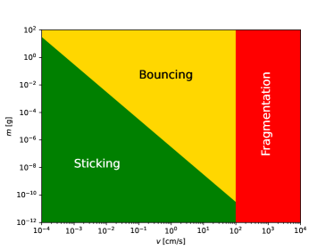
Figure 1: Sticking-bouncing-fragmentation diagram showing in which parts of the parameter space equal-mass collisions lead to one of the three outcomes. This figure is the direct equivalent of Fig. 11 of Güttler et al. (2010), with $F_{\mathrm{roll}}=10^{-4}$ dyne, $a_{\mathrm{mono}}=1\,\mu$m, and $v_{\mathrm{f}}=100$ cm/s.

Following Windmark et al. (2012b) and Stammler & Birnstiel (2022), we computed the probability of sticking, bouncing, and fragmentation for any pair of dust particle masses $(m_{1},m_{2})$ by assuming that the relative velocities of these dust particles obey a Maxwell-Boltzmann distribution defined as

$${\cal P}_{\mathrm{MB}}(\Delta v)=3\sqrt{\frac{6}{\pi}}\,\frac{\Delta v^{2}}{v_{\mathrm{rms}}^{3}}\,\exp\left(-\frac{3}{2}\frac{\Delta v^{2}}{v_{\mathrm{rms}}^{2}}\right),$$ (6)

where $v_{\mathrm{rms}}$ is the root-mean-square of the relative velocities. The probability of a collision between these two dust particles with a relative velocity greater than a given value $v$ is then

$$P(\Delta v>v)=\int_{v}^{\infty}{\cal P}_{\mathrm{MB}}(\Delta v)d\Delta v=\left(\frac{3}{2}\frac{v^{2}}{v_{\mathrm{rms}}^{2}}+1\right)\exp\left[-\frac{3}{2}\frac{v^{2}}{v_{\mathrm{rms}}^{2}}\right]$$ (7)

(see Eq. 10 of Stammler & Birnstiel, 2022). By setting $v=v_{\mathrm{f}}$ in Eq. (7), we obtained the probability that a collision leads to fragmentation. By setting $v=v_{\mathrm{b}}$ in Eq. (7), we obtained one minus the probability that a collision leads to sticking. This is illustrated in Fig. 2.

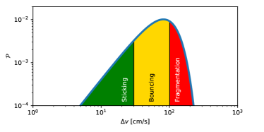
Figure 2: Assumed Maxwell-Boltzmann-like distribution function for the relative velocities between colliding dust particles and the three regimes of collisional outcomes. This figure is the direct equivalent of Fig. 6-Left of Stammler & Birnstiel (2022), with $v_{\mathrm{b}}=30$ cm/s and $v_{\mathrm{f}}=100$ cm/s.

Without bouncing, these two probabilities add up to unity. However, with bouncing, they add up to a value below unity. The remainder is the probability of bouncing. Since bouncing does not change the mass distribution of the dust, the mere fact that the probabilities of sticking and fragmentation do not add up to one implies that the bouncing barrier is implemented. Bouncing is simply a reduction of the effective collision rate. In the Appendix D, we give Python code snippets that we used to implement this bouncing barrier model in DustPy.

3.2 Estimation of the bouncing barrier

Under the assumption that turbulence is the dominant cause of relative velocities between dust grains, Birnstiel et al. (2012) formulated analytic estimates of the growth mass limits due to fragmentation and radial drift and showed them to be good predictors for the upper envelope of the grain size distribution. The largest Stokes number the grains acquire is given by

$$\mathrm{St}_{\mathrm{f}}=\frac{1}{3}\frac{v_{\mathrm{f}}^{2}}{\alpha c_{\mathrm{s}}^{2}},$$ (8)

where $c_{\mathrm{s}}$ is the isothermal sound speed of the gas and $\alpha$ is the usual turbulence parameter. According to Birnstiel et al. (2010), the radius $a$ and the Stokes number $\mathrm{St}$ are related via

$$\mathrm{St}=\frac{\rho_{\bullet}a}{\Sigma_{\mathrm{g}}}\,\frac{\pi}{2},$$ (9)

where $\Sigma_{\mathrm{g}}$ is the surface density of the gas in the disk and $\rho_{\bullet}$ is the material density of the dust grain, assuming a spherical grain geometry and with porosity included. Solving Eq. (8) for $a$, we obtained the grain size limit due to fragmentation:

$$a_{\mathrm{f}}=\frac{2}{3\pi}\frac{\Sigma_{\mathrm{g}}v_{\mathrm{f}}^{2}}{\alpha\rho_{\bullet}c_{\mathrm{s}}^{2}}.$$ (10)

For the bouncing barrier, we suggest a similar formula:

$$\mathrm{St}_{\mathrm{b0}}=\frac{1}{3}\frac{v_{\mathrm{b}}^{2}}{\alpha c_{\mathrm{s}}^{2}},$$ (11)

where $v_{\mathrm{b}}(m)=v_{\mathrm{b}}(m,m)$ (i.e., we assume equal-sized collisions). This is a pessimistic estimate because in a collision, strongly unequal-sized particles are more likely to stick than particles of equal size, as one can see from Eq. (3). However, as shown below, once the bouncing barrier becomes dominant, the dust distribution becomes rather narrow, meaning that collisions of similar-sized particles become the most common. We note that we added a zero to $\mathrm{St}_{\mathrm{b0}}$ because as we show later (Eqs. 13,14 and the red dotted line in Fig. 3), this estimate has to be modified due to the Kolmogorov cutoff scale. However, we initially ignore this effect. Equation  (11) is an implicit equation for the bouncing barrier limit on the grain size because both the Stokes number $\mathrm{St}$ and the bouncing velocity $v_{\mathrm{b}}$ depend on the grain mass $m$. The dust grain mass $m$ and radius $a$ are related via $m=4\pi\rho_{\bullet}a^{3}/3$, allowing us to express $v_{\mathrm{b}}(m)$ in terms of $a$. Then solving Eq. (11) for $a$, we obtained the grain size limit due to bouncing:

$$a_{\mathrm{b0}}=\left(\frac{5}{\pi}\frac{\Sigma_{\mathrm{g}}a_{\mathrm{mono}}F_{\mathrm{roll}}}{\alpha c_{\mathrm{s}}^{2}\rho_{\bullet}^{2}}\right)^{1/4}.$$ (12)

Apparent from this equation is the fact that the bouncing barrier is rather insensitive to the disk parameters, such as $\alpha$ and $\Sigma_{\mathrm{g}}$, due to the one-fourth power dependency. When $\alpha$ is increased by a factor of ten, the bouncing barrier grain size $a_{\mathrm{b0}}$ decreases by only 15%. The fragmentation barrier (Eq. 10) does not have this one-fourth power dependency. Thus, when $\alpha$ is increased by a factor of ten, the fragmentation barrier grain size $a_{\mathrm{f}}$ decreases by a factor of ten. As we later show, this has the consequence that for a high $\alpha$, the fragmentation becomes important, while for a low $\alpha$, the grain growth is stopped by the bouncing barrier before reaching the fragmentation barrier. We also show that this has interesting consequences for models of chondrule formation (Section 5.6).

However, it turns out that this estimate of the grain size of the bouncing barrier is often too small because the Kolmogorov turbulence cascade does not continue to small enough eddies. This problem rarely happens when computing the fragmentation barrier because that occurs at rather large velocities. Yet it becomes important for the bouncing barrier. In the turbulence model of Ormel & Cuzzi (2007), the Kolmogorov scale is computed as follows: The gas of the disk is assumed to be dominated by H₂ molecules, which have a mutual collisional cross section of $\sigma_{\mathrm{H}_{2}}=2\times 10^{-15}\,\mathrm{cm}^{2}$. The mean molecular weight is assumed to be $\bar{m}=2.3\,m_{\mathrm{p}}$, where $m_{\mathrm{p}}$ is the proton mass. This leads to a mean free path of the gas particles of $\lambda_{\mathrm{mfp}}=\bar{m}/\rho_{\mathrm{g}}\sigma_{\mathrm{H}_{2}}$, where $\rho_{\mathrm{g}}$ is the gas volume density. The thermal velocity of the gas particles is $v_{\mathrm{th}}=\sqrt{8k_{\mathrm{B}}{}T/\pi\bar{m}}=\sqrt{8/\pi}\,c_{\mathrm{s}}$, where $k_{\mathrm{B}}{}$ is the Boltzmann constant and $T$ is the temperature of the gas. This leads to a molecular viscosity of $\nu_{\mathrm{mol}}=v_{\mathrm{th}}\lambda_{\mathrm{mfp}}/2$. The Reynolds number of the largest eddies is Re = $\alpha c_{\mathrm{s}}h_{p}/\nu_{\mathrm{mol}}$, where $h_{p}=c_{\mathrm{s}}/\Omega_{\mathrm{K}}$ is the scale height of the disk, with $\Omega_{\mathrm{K}}$ the Kepler frequency. The turnover timescale of the eddies at the Kolmogorov scale becomes $t_{\eta}=(\Omega_{\mathrm{K}}\sqrt{\mathrm{Re}})^{-1}$. The grain size coupling to these smallest eddies is then

$$a_{\eta}=\frac{\rho_{\mathrm{g}}\sqrt{8/\pi}c_{\mathrm{s}}t_{\eta}}{\rho_{\bullet}}=\frac{\rho_{\mathrm{g}}c_{\mathrm{s}}}{\rho_{\bullet}\Omega_{\mathrm{K}}}\sqrt{\frac{8}{\pi\,\mathrm{Re}}}\quad.$$ (13)

The grain size of the bouncing barrier is then

$$a_{\mathrm{b}}=\max(a_{\mathrm{b0}},a_{\eta})\quad.$$ (14)

In Section 4, in Fig. 3, the red solid an dotted lines show the difference this makes for our fiducial model.

We note that Gong et al. (2021) propose a modification of the turbulent stirring model of Ormel & Cuzzi (2007), which may better describe the turbulence produced by the magneto-rotational instability. In their model, the Kolmogorov cutoff scale is at a smaller Stokes number, and the relative velocities between particles are generally larger. This would push the bouncing barrier toward smaller aggregate sizes.

Table 1: Model parameters.

Series	Model name	$M_{\mathrm{disk}}\;[M_{\odot}]$	$\alpha$	$s\;[\mathrm{cm}]$	BB
$\alpha$	m2_a3_s4_nobo	$10^{-2}$	$\mathbf{10^{-3}}$	$10^{-4}$	no
fiducial	m2_a4_s4_nobo	$\mathbf{10^{-2}}$	$\mathbf{10^{-4}}$	$\mathbf{10^{-4}}$	no
$\alpha$	m2_a5_s4_nobo	$10^{-2}$	$\mathbf{10^{-5}}$	$10^{-4}$	no
$\alpha$	m2_a6_s4_nobo	$10^{-2}$	$\mathbf{10^{-6}}$	$10^{-4}$	no
misc	m1_a4_s4_nobo	$\mathbf{10^{-1}}$	$10^{-4}$	$10^{-4}$	no
misc	m2_a4_s5_nobo	$10^{-2}$	$10^{-4}$	$\mathbf{10^{-5}}$	no
$\alpha$	m2_a3_s4	$10^{-2}$	$\mathbf{10^{-3}}$	$10^{-4}$	yes
fiducial	m2_a4_s4	$\mathbf{10^{-2}}$	$\mathbf{10^{-4}}$	$\mathbf{10^{-4}}$	yes
$\alpha$	m2_a5_s4	$10^{-2}$	$\mathbf{10^{-5}}$	$10^{-4}$	yes
$\alpha$	m2_a6_s4	$10^{-2}$	$\mathbf{10^{-6}}$	$10^{-4}$	yes
misc	m1_a4_s4	$\mathbf{10^{-1}}$	$10^{-4}$	$10^{-4}$	yes
misc	m2_a4_s5	$10^{-2}$	$10^{-4}$	$\mathbf{10^{-5}}$	yes

Note: The name (column 2) was constructed from minus the exponents of the values in columns 3, 4, and 5, respectively. Column 3 is the disk gas+dust mass in units of solar mass. Column 4 is the turbulence parameter $\alpha$. Column 5 is the monomer size $s$ in units of centimeters. Column 6 lists whether the bouncing barrier was included in the model or not. The full rows for the models m2_a4_s4_nobo and m2_a4_s4 are in bold to indicate that these are the fiducial models. For the other models, we have made bold the parameter that deviates from the fiducial model. Column 1 shows to which series the model belongs (for the discussion, we refer to Sec. 4).

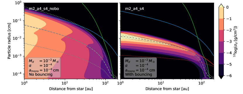
Figure 3: Dust size distribution for the fiducial model without the bouncing barrier m2_a4_s4_nobo (left) and with bouncing barrier m2_a4_s4 (right). The blue line is the fragmentation barrier, the green line is the radial drift barrier, and the red line is the bouncing barrier, all computed assuming turbulence to be the dominant driver of relative velocities. The dotted red line is the bouncing barrier if Eqs. (13,14) are not taken into account. The dashed gray line is the mean grain size, and the dotted lines are plus or minus one standard deviation in log space (see Appendix A.1). The color scale denotes the surface density of the dust $\sigma_{\mathrm{d}}(r,m)=m\,\Sigma_{\mathrm{d}}(r,m)$ in units of grams per square cm² per $\ln(m)$.

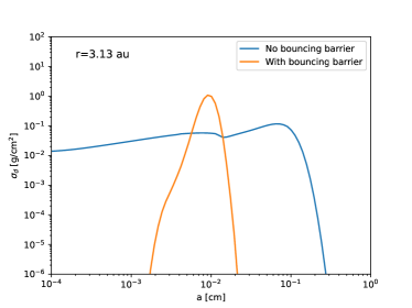
Figure 4: As in Fig. 3 but now with a slice at $r=3.13$ au.

4 Results

In this section, we describe the parameters used in our computations. We then show the results.

4.1 Model parameters

As an initial condition, we set up a protoplanetary disk with the usual power law plus cutoff shape,

$$\Sigma_{\mathrm{g}}(r)=\Sigma_{0}\,\left(\frac{r}{r_{0}}\right)^{-1}\exp\left(-\frac{r}{60\,\mathrm{au}}\right),$$ (15)

around a solar-type star. The initial dust-to-gas ratio is 0.01. We chose $\Sigma_{0}$ and $r_{0}$ such that the mass of the disk is a given value $M_{\mathrm{disk}}$, where $M_{\mathrm{disk}}$ is a parameter we varied. Other parameters we varied are the turbulent strength $\alpha$ and the monomer radius $s$. The radial $r$ grid is between $r_{\mathrm{in}}=1\,\mathrm{au}$ and $r_{\mathrm{out}}=10^{3}\,\mathrm{au}$ with $N_{r}=$100 logarithmically spaced radial bins. The coagulation was computed on a mass grid between $m_{\mathrm{min}}=10^{-12}\,\mathrm{g}$ and $m_{\mathrm{min}}=10^{5}\,\mathrm{g}$ with 120 logarithmically spaced bins. The material density was taken to be $\rho_{\bullet}=1.67\,\mathrm{g}\,\mathrm{cm^{-3}}$. The fragmentation velocity was set at 100 cm/s and scaled only when the monomersize was varied, using Eq. (2). The fragment distribution function is the standard power law $f(m)\propto m^{-11/6}$, which is identical to the Mathis-Rumple-Nordsieck (MRN, Mathis et al., 1977) size distribution. The models were run for $10^{6}$ years, and we show the results for the final time frame at $t=10^{6}$ years.

The parameter space spanned up by $M_{\mathrm{disk}}$, $\alpha$, and $s$ was explored in steps of ten. The parameter values are listed in Table 1.

4.2 Fiducial model

To discuss our results, we chose as our fiducial model the model with $M_{\mathrm{disk}}=10^{-2}M_{\odot}$, $a_{\mathrm{mono}}=10^{-4}\,\mathrm{cm}$ and $\alpha=10^{-4}$ (model m2_a4_s4). For comparison, we also discuss the results of model m2_a4_s4_nobo, which is the same model but without the bouncing barrier.

To analyze the results of the models, we computed a number of quantities at each radius $r$ from the local dust size distribution: the mean and the width of the distribution, the vertical optical depths, the mean degree of settling, the number of collisions per megayear, and the mean collisional velocity. Furthermore, images at two wavelengths were computed. The details of how these quantities and images were computed are described in the Appendix A.

The comparison between the non-bouncing and the bouncing versions of the fiducial model are shown in Fig. 3. The original DustPy model without the bouncing barrier is shown on the left, and the new model with the bouncing barrier is shown on the right. A slice of the same data at $r=3.13$ au is shown in Fig. 4 in a log-log figure.

Two main effects of the bouncing barrier are immediately obvious from these figures. One is that the grains stop growing at a smaller grain size, in this case up to a factor of ten in radius or 1000 in mass. The other is that the grain size distribution becomes very narrow, almost monodisperse. This is very different from the almost flat distribution created by the growth-fragmentation steady state in the model without bouncing. At the outer edge of the disk, the drift barrier still plays a role. Inward of 100 au, the bouncing barrier determines the grain size distribution. We anticipate that this may have consequences for the growth speed of the streaming instability and for the accretion rate and efficiency of pebble accretion. We discuss these consequences in more detail in Sec. 5.5.

Figure 5: Mean collision velocities in the fiducial model. Left: Without bouncing. Right: With bouncing.

Figure 6: As in Fig. 5-right but this time using the mean collision velocities instead of the Maxwell-Boltzmann distribution for the relative velocities.

Figure 7: Mean number of collisions that a dust particle experiences over the course of $10^{6}$ years in the fiducial model. Left: Without bouncing. Right: With bouncing.

Figure 8: Vertical optical depth of the disk at two wavelengths in the fiducial model. Left: Without bouncing. Right: With bouncing. Shown as the dashed brown line is the average degree of dust settling. This line uses the axis labeling on the right-hand side of the plot.

Figure 5 shows the mean collision velocities that appear in the model calculations. In both cases, the velocities are dominated by turbulent motions, except for the outermost parts of the disk. As expected, the mean collision velocities in the model without bouncing get close to the fragmentation barrier. The fragmentation happens at the upper end of the size distribution, where the relative velocities are the highest. When the bouncing barrier is included in the model, the collision velocities are reduced significantly because the grains do not grow as big as without the bouncing barrier. It is noteworthy that the collision velocities exceed the bouncing velocity (purple curve) significantly. This is because the Maxwell-Boltzmann velocity distribution (Eq. 6) always has a non-zero probability for collisions with a velocity that is sufficiently low for growth to be possible. The bouncing barrier therefore never completely inhibits growth, although the larger the grains grow, the less likely it is that a collision leads to growth. The size distribution therefore tends to ”overshoot” the estimated bouncing barrier somewhat. To verify this effect, we show in Fig. 6 the same model but with the Maxwell-Boltzmann velocity distribution replaced with the mean velocity, for both the bouncing barrier and the fragmentation barrier. We found that in this case the mean collision velocity is substantially closer to the analytic expectation, confirming our suspicion. We also did an experiment where we switched off the fragmentation completely just to be sure that a small amount of fragmentation of some grains could not lead to the growth of others through accretion of small dust grains. But as expected, because the fragmentation barrier is so much above the bouncing barrier in this model, the experiment did not show any difference, demonstrating that fragmentation does not play a role in this overshoot phenomenon.

When dust aggregates ”hit” the bouncing barrier, their growth is inhibited, but they continue to regularly collide with each other. We demonstrate this in Fig. 7 by computing the number of collisions per megayear. With the exception of the outer edge of the disk, the number of collisions is significant everywhere, from hundreds to about one hundred thousand. We therefore expected that the dust aggregates in the bouncing barrier would be gently compressed by the many collisions over the course of their evolution, similar to what was demonstrated in the model of Zsom et al. (2010).

The fact that the size distribution becomes so narrow in the bouncing case, as seen in Figs. 3 and 4, opens up the question if the observational appearance of disks would be strongly modified by this process. In order to assess this, we computed the vertical optical depth in the H band (1.65 $\mu\mathrm{m}$) and at ALMA Band 6 (1.3 mm) wavelengths. The results are shown in Fig. 8. Maybe somewhat surprisingly, the optical depth of the disk is not very strongly affected by this change. For the ALMA wavelengths, this is caused by the fact that the particles are not much larger than the observation wavelength in either case, so the observations mostly probe the mass and not the surface of the grains. Also shown in Fig. 8 is the average degree of dust settling. In both simulations, $H_{\mathrm{d}}/H_{\mathrm{g}}$ slowly decrease as a function of distance from the star, with typical values of a few times 10^-1.

We computed images at submillimeter and near-IR wavelengths using RADMC-3D (Dullemond et al., 2012). Dust opacities were computed with optool (Dominik et al., 2021). For details on the dust opacities, see Section A.2. For the vertical distribution of the different dust grain sizes, we used the formula given by Equations 24 and 25 in Fromang & Nelson (2009). Figure 9 shows an edge-on ALMA view of our disk models. The model including bouncing is slightly thinner because of the strong reduction in smaller grains that would diffuse up vertically under some degree of turbulence. Apart from the difference in thickness, the images are very similar.

For the shorter wavelength, the optical depth is reduced by a factor of 10-100 but not nearly enough to render the disk optically thin. There is nevertheless a very significant effect on the appearance of the disk in high contrast scattered light images, as shown in Fig. 10. Here, bouncing leads to a strong depression of the surface brightness in the range between 50 and 80 au. This darkening is caused by shadowing. In the inner disk, the grains are sufficiently coupled to the gas to create a region of higher aspect ratio. In the dark region, the absence of micron-sized grains means that the settling of all dust is sufficient to fall into the shadow cast by the inter region, creating what looks like a gap. Beyond 80 au, for the case with bouncing, the disk flaring in combination with the small grain sizes at large distances cause the disk surface to climb out of the shadow again. The effect is the opposite in the model without bouncing because small grains are present everywhere. The inner disk becomes effectively thicker, and the disk flares nicely to a distance of about 60 au. Farther away from the star, the upper layers of the disk do become optically thin and fall into the shadow created by the inner- and middle-disk regions.

The effect that the outer disk, or part of it, is shadowed by the inner disk is often called ”self-shadowing” because the disk casts a shadow onto itself (Dullemond & Dominik, 2004). Such an effect is commonly seen in observations of protoplanetary disks (Garufi et al., 2022), although it is usually considered in the context of a disk’s inner rim casting the shadow.

The removal of small grains also impacts the spectral energy distribution (SED) of the disk. This effect is shown in Fig. 11. In the model with the bouncing barrier turned on and fully effective, the 10 and 20 $\mu{}$m silicate features that are very prominent in the no-bouncing model disappear entirely. The SED at mid-IR wavelengths becomes significantly weakened, as the area of the disk where much of this radiation normally originates from becomes shadowed and colder. It is possible that the effectiveness of small grain removal is too large in our bouncing model. The many collisions in the bouncing regime may have an erosive component that would put small amounts of small grains back into the gas. Also, in disks with very low turbulence, the basic assumption of DustPy that full vertical mixing is always available and fast may be incorrect so that small grains are able to stay suspended higher in the disk atmosphere for a much longer time. Only models that treat the vertical structure of disks self-consistently are able to address this point.

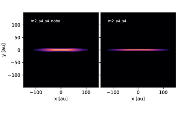
Figure 9: Synthetic image of the disk of the fiducial model seen edge-on ($i=90^{\circ}$) at a wavelength $\lambda=1.3$ mm.

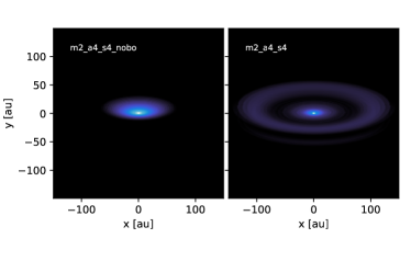
Figure 10: Synthetic image of the disk of the fiducial model seen at an inclination $i=70^{\circ}$ and at a wavelength $\lambda=1.65\mu$m.

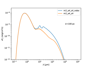
Figure 11: Spectral energy distribution of the fiducial model with and without bouncing.

In the following sections, we look at small parameter studies that illuminate the effects of key model parameters. These parameters include the turbulent strength $\alpha$, the monomer size $a_{\mathrm{mono}}$, and the disk mass $M_{\mathrm{disk}}$.

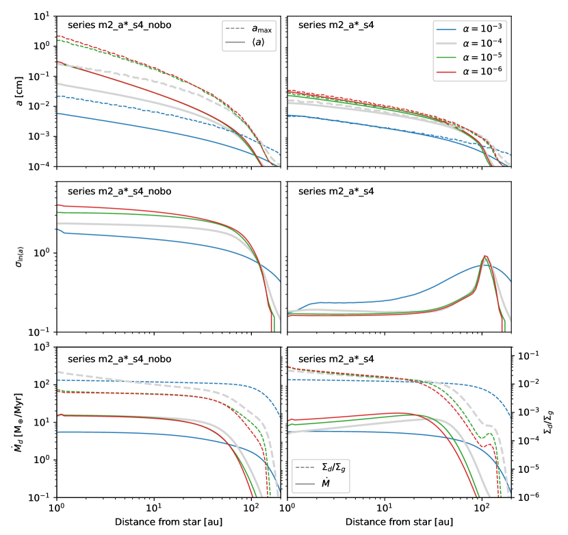
Figure 12: Mean particle radius, width of the distribution, maximum grain size (all defined in section A.1), and dust accretion rate for the m2_a*_s4 series. The asterisk ($*$) stands for 3, 4, 5, or 6, meaning varying turbulence parameter $\alpha=10^{-3,4,5,6}$. The gray curves denote the fiducial model (m2_a4_s4). Left: Without bouncing. Right: With bouncing.

4.3 Model series with varying turbulent strength

We first look at the effect of the turbulent strength on the model result. Turbulent strength is a key parameter since there is much uncertainty about it currently in the literature. The few available measurements indicate values $\alpha\la 2\times 10^{-3}$ (e.g., Flaherty et al., 2015; Teague et al., 2016), but much lower values are very seriously considered. For this section, we have computed models with $\alpha$ values of $10^{-3}$, $10^{-4}$, $10^{-5}$, and $10^{-6}$. The full set of parameters for these models can be found in Tab. 1.

Turbulence is a key factor in the collisional dust growth scenario. It is a source of relative velocities that may, depending on strength, dominate the relative velocities of grains. Turbulence also determines the vertical and radial spreading of the spatial distribution of grains.

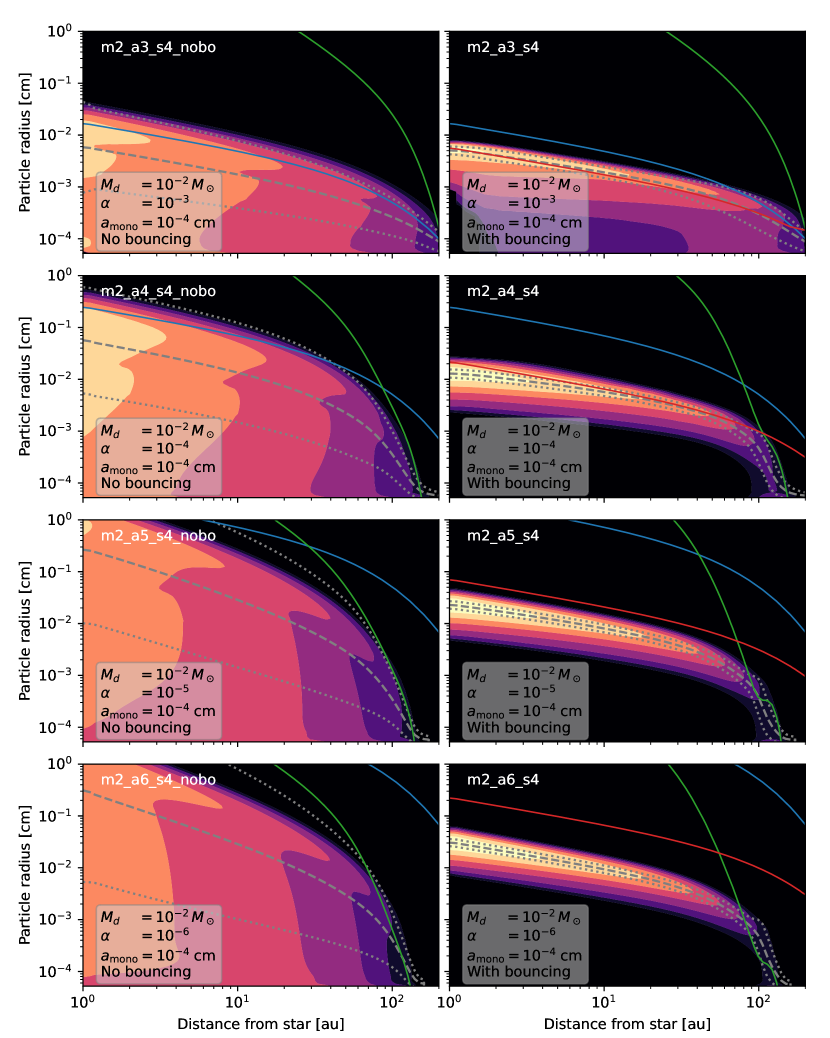
Figure 16: Dust surface densities for the turbulence series (Section 4.3). Left: Turbulence series without bouncing. Right: Turbulence series with bouncing.

The full size distribution plots for these runs are available for reference in Fig. 16 in the Appendix. Here, in Fig. 12, we document the influence of changing turbulence strength on the dust size distribution present after a megayear in a disk. In all plots, the gray curve represents the fiducial models discussed in Section 4.2. The blue curve is a model with a higher turbulence, $\alpha=10^{-3}$. The green and red curves represent the weak turbulence cases for $\alpha=10^{-5}$ and $\alpha=10^{-6}$. In the figure, the upper row shows the average grain size (solid curves) and the upper limit (dashed curves) at each location of the disk. Without bouncing, there is a clear progression of the mean size, increasing as the turbulence gets weaker. However, the curves for 10^-5 and 10^-6 are identical. This happens because at such low $\alpha$, the collision velocities are determined by radial drift and no longer by turbulence. In the case with bouncing, the mean dust size starts to stagnate at around 100 $\mu\mathrm{m}$, indicating that radial drift already starts to take over for these smaller grains already at $\alpha=10^{-4}$, the fiducial model.

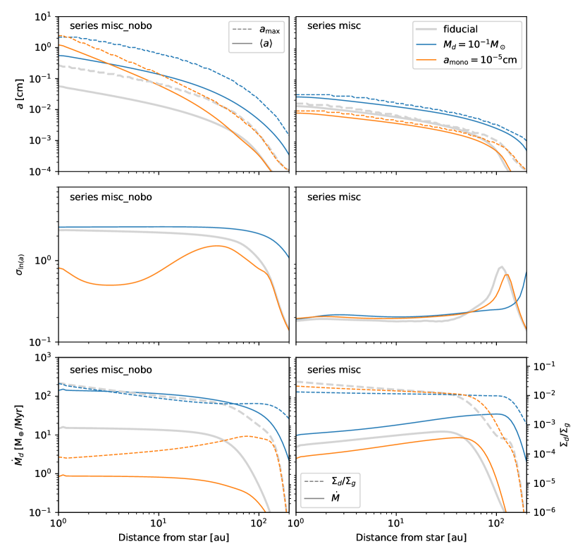
Figure 13: Mean particle radius, width of the distribution, and dust accretion rate for the mixed series. Left: Without bouncing. Right: With bouncing.

The enormous differences in the width of the size distributions become visible in the middle row of plots in Fig. 12. Without bouncing, we get a large logarithmic width of the distribution that becomes larger with a smaller turbulence, owing to the fact that the maximum grain size keeps increasing, while fragmentation continues to replenish very small grains. In the case with bouncing, all but one model have a very narrow distribution with a logarithmic width of only 0.2. Only the largest considered value for the turbulence manages to widen the distribution a bit because bouncing and fragmentation barriers move closer together, and the occasional outlier in the collision velocity produces some fragments. This effect can be seen in Fig. 16, where the fragmentation barrier has moved down because of the increased relative velocities caused by turbulence. The widths of the distributions peak at the outer disk edge, where growth times are slow and the drift barrier plays a role.

Finally, the bottom row of plots in Fig. 12 shows the dust mass accretion $\dot{M}_{\mathrm{d}}$, often referred to as the ”pebble flux,” as a function of distance. Here, we can also make interesting observations. In the models without bouncing, the pebble flux reaches a constant, steady state value over much of the disk. The flux is about 15 Earth masses per megayear. In the model with the highest turbulent speed, the value drops to 5 Earth masses per Myr because the more violent turbulence keeps a larger fraction of the mass in smaller grains that drift more slowly. The plot for the computation with bouncing shows a noticeable difference. The flux in the $\alpha=10^{-3}$ models is quite similar to the no-bouncing case. However, for the smaller values of alpha (leading to a very narrow size distribution), the pebble flux is decreases toward the star ($d\dot{M}_{\mathrm{d}}/dr>0$). What can be seen here is a traffic jam effect that leads to an increase of the dust surface density and therefore an increase of the metallicity of the disk as one gets closer to the star.

4.4 Model series with miscellaneous varying parameters

Next, we explore two other key parameters of the models: the disk mass $M_{\mathrm{disk}}$ and size of the monomer. A high disk mass is often used to dial into the right conditions for making the streaming instability and pebble accretion possible and effective. The monomer size has an influence on the stability of aggregates and therefore on the fragmentation velocity via Eq. (2), so a factor of ten reduction in monomer size leads to a very significant increase of the fragmentation velocity by a factor of 6.8.

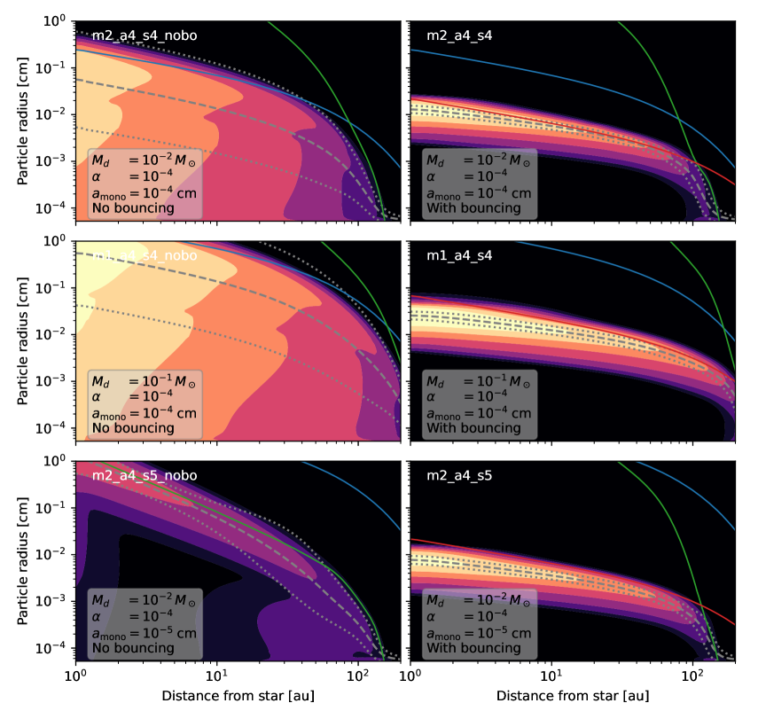
Figure 17: Dust surface densities for the miscellaneous series (Section 4.4). Left: Miscellaneous series without bouncing. Right: miscellaneous series with bouncing.

The full size distribution plots for these runs are available for reference in Fig. 17 in the Appendix. Here, in Fig. 13, we show again the fiducial model (gray line), a model where the disk mass is increased by a factor of ten to $10^{-1}M_{\odot}$, and another model where we decrease the monomer size. The full set of parameters for these models can be found in Tab. 1.

In the non-bouncing case, one can see that both increasing the disk mass and reducing the monomer size leads to an increase of the mean and maximum grain sizes. With a larger disk mass, grains are better coupled, and collision velocities are reduced. With a smaller monomer size, aggregates are more rigid and harder to fragment, an effect explaining the rise of the mean and maximum particles in this context. An interesting effect happens with the width of the size distribution. The width remains large with an increased disk mass. But in the computation with the small monomers, the size distribution suddenly becomes very narrow, and it drops to a value of $\sim 0.45$. The explanation goes as follows: The fragmentation velocity increases by a factor of 6.8, so the aggregates are allowed to grow to much larger sizes. But also the fragmentation velocity is now larger than the drift barrier velocity so that the size distribution is now set by the drift barrier. In that setting, a narrow size distribution is expected (Birnstiel et al., 2011).

The changes in disk mass and monomer size have much less effect on the outcome in the models with bouncing included. The mean and maximum size increase by about a factor of two for the massive disk, while they are reduced by a factor less than two in the small monomer case. The size distributions remain narrow, indicating that in both cases, bouncing is what sets the size distribution to almost monodisperse.

The last row of Fig. 13 shows the effect on the dust mass accretion rate (i.e., the pebble flux). The changes to the pebble flux in the non-bouncing models are very large. In the massive disk, the pebble flux is increased by almost an order of magnitude simply because the surface density of the disk (and consequently of the dust) is also a factor of ten higher. The model with small monomers shows a small pebble flux after 1 Myr because the drift has been extremely effective and the disk is already emptied out, as most dust has already moved into the innermost disk and evaporated. In the models with bouncing, the variations are much more moderate, pebble fluxes change only by a factor of less than two. This is a critically important observation. It may mean that when the bouncing barrier is active, increasing the disk mass is no longer the automatic fix to create the very large pebble fluxes that are required in many global planet formation models (e.g., Lambrechts et al., 2019; Bitsch et al., 2019; Izidoro et al., 2021).

5 Implications and discussion

We have shown that introducing the bouncing barrier into global models of dust evolution does significantly modify the models and changes grain sizes and grain distributions. In this section, we look at the different areas in the context of planet formation models where these changes may have consequences.

5.1 Retaining dust in disks for longer

The issue of retention of dust in disks has long been considered an important aspect of disk models. If dust grains are allowed to grow too quickly into the planetesimal regime and beyond, one would expect the dust masses measured with an instrument such as ALMA to decrease on the same timescale. If dust growth instead stops near sizes defined by Stokes numbers close to unity, these particles are expected to drift toward the star on a timescale of $\sim 100$ local orbital timescales. Those timescales are too short based on the fact that we do observe massive disks out to lifetimes of 3-20 Myr. In addition, observations seemed to show for a long time that the particles in disks are indeed mittimetre to centimetre in size (e.g., Wilner et al., 2005), which would have a fast drift as an unavoidable property. Besides dust traps (Pinilla et al., 2012) or extreme porosities (Kataoka et al., 2013), the key mechanism to allow the observations to be consistent with model predictions is to limit particle growth. The various growth barriers prevent direct growth to planetesimal sizes and keep the dust in a size range where an instrument like ALMA is maximally sensitive (Birnstiel et al., 2010). Also, it has become clear now that the effects of optical depth can mimic very large grain sizes even if the grains themselves are somewhat smaller (Testi et al., 2014; Guidi et al., 2022). This has been confirmed by modeling polarization by self-scattering (Kataoka et al., 2016). Through a deep analysis of HD 163296 with multi-wavelength observations from ALMA and the Karl Janski array, Guidi et al. (2022) showed that the grain sizes in the outer regions of this disk are on the order of 0.2 mm. While a fragmentation velocity of 1 m/s goes a long way to solving the problem of dust retention (Birnstiel et al., 2009), the bouncing barrier is very effective in decreasing the particle sizes further and retaining dust for longer. We observed this in Fig. 12, where the 1 Myr dust surface density is a factor of five higher in low-turbulence models with the bouncing barrier compared to models where the barrier is absent. Therefore, we concluded that the bouncing barrier can help keep dust surface densities higher for longer.

5.2 Modification of trapping efficiency

Particles can be captured in pressure bumps that act as particle traps (e.g., Paardekooper & Mellema, 2004; Rice et al., 2006; Paardekooper & Mellema, 2006; Pinilla et al., 2012, 2012). A trap with any given pressure contrast can store particles in a given size range. Smaller particles can be extracted by turbulent mixing and a continuing accretion flow of gas. Strong fragmentation can make a dust trap ”leaky” because the small grains produced by the fragmentation leak out of the dust trap (Stammler et al., 2023).

The bouncing barrier can affect the trapping efficiency in two ways. On the one hand, it reduces the maximum particle size. If the particle size set by fragmentation is such that the particles would only be weakly trapped, then the bouncing barrier can make the trap leaky, even for the largest grains present. On the other hand, the bouncing barrier leads to a strong depletion of small micron-sized dust. Such small particles are normally strongly coupled to the gas and form a component that can be pulled out of a trap by viscous mixing. Therefore, the bouncing barrier will make traps less leaky for small grains but possibly more leaky for the largest grains present in the disk.

5.3 Abundance of small grains, optical depth, and scattered light images

An active bouncing barrier produces a narrow size distribution. One consequence of this is that the amount of small grains should be reduced to the extent that they may be completely absent. We have shown that this is indeed what our simple bouncing barrier model predicts.

This may seem to contradict observations of protoplanetary disks at optical and mid-IR wavelengths, which do contain signatures of some amount of small grains. The disk does not become optically thin by this removal of small grains (Dullemond & Dominik, 2005) because the upper limit of the size distribution (and also the mean) remain at sizes of typically 100 $\mu\mathrm{m}$, rendering the disk optically thick at both optical and mid-IR wavelengths. However, we have shown that the strong reduction in the abundance of small, $\mu\mathrm{m}$-sized grains can significantly change the appearance of the disk in scattered light by depressing parts of the disk into the shadow produced by inner disk regions. Also, if the disk consists entirely of 100 $\mu\mathrm{m}$-sized dust aggregates that are moderately compacted by bouncing, then we should expect that the mid-IR spectrum does not show a 10-$\mu\mathrm{m}$ silicate feature, which is contrary to the fact that most disks in fact show a strong 10-$\mu\mathrm{m}$ silicate emission feature in their spectrum (Meeus et al., 2001; Furlan et al., 2006; Kessler-Silacci et al., 2006).

A perfect bouncing barrier without any production of small collisional debris may therefore be hard to reconcile with observations of protoplanetary disks. On the other hand, the fact that we find that each dust aggregate bounces hundreds to thousands of times against other aggregates during the lifetime of the disk (see Fig. 7) suggests that even a small amount of abrasion during these collisions will go some way to replenishing the reservoir of small grains. Follow-up studies therefore should use these observational constraints to determine how much abrasion is necessary to keep consistent with observations and whether this will effectively eliminate the bouncing barrier or not. A further possibility to consider is that vertical mixing may not be as fast as assumed in DustPy. Thus, some small grains may remain in the disk atmosphere for a long time in a more or less primordial state, as seems to be indicated by a careful analysis of the dust in the upper layers of the IM Lup disk (Tazaki et al., 2023).

5.4 Vertical height of the dust disk

Observations of edge-on planet-forming disks with ALMA have revealed that the midplane of the disk, supposedly composed of large grains in the millimetre to centimetre range, is very geometrically thin. Pinte et al. (2016) constrained the aspect ratio of the rings in the HL Tau disk to about $H_{\mathrm{d}}/r\simeq 0.01$. Villenave et al. (2022) measured the ratio of the dust and gas scale heights in the disk of Oph 163131 to be $H_{\mathrm{d}}/H_{\mathrm{g}}\simeq 5\times 10^{-2}$. Dubrulle et al. (1995) and Birnstiel et al. (2010) showed that for Stokes numbers less than one, the vertical width $H_{\mathrm{d}}$ will be related to the ratio of the turbulent strength and the Stokes number by

$$\frac{H_{\mathrm{d}}}{H_{\mathrm{g}}}=\min\left(1,\sqrt{\frac{\alpha}{\mathrm{St}}}\right)\quad.$$ (16)

Since the bouncing barrier reduces the upper limit of the size distribution, and therefore the Stokes number of those grains, a model with the bouncing barrier will place even more stringent constraints on the turbulent mixing available. For our modeling grid with varying turbulent strength, we show the ratio $H_{\mathrm{d}}/H_{\mathrm{g}}$ in Fig. 14. To reach the measured thickness of the Oph 163131 disk, we would require $\alpha\la 10^{-5}$. We note that his specific result still depends on the adopted gas surface density.

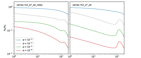
Figure 14: Ratio of the dust scale height to the gas scale height for models with different turbulent strengths. Left: Without the bouncing barrier. Right: With the bouncing barrier.

5.5 Streaming instability and planetesimal formation, pebble accretion

The streaming instability is currently the favorite model to explain the formation of planetesimals. In order to activate the streaming instability, a number of criteria need to be fulfilled. Roughly speaking, these criteria are (1) the local metallicity of the disk, which must be (depending on the study) not too far below solar (Li & Youdin, 2021) or significantly above solar (Johansen et al., 2009), and (2) the Stokes number of the pebbles drifting through the gas. Stokes numbers between 10^-3 and 1 have been reported to be effective. These criteria apply strictly to laminar disks. For a disk that has active turbulence, the efficiency of the streaming instability can be reduced or even become zero if grains are not allowed to settle to the midplane (Gole et al., 2020). Recently, there has been a lot of discussion on the effects of a polydisperse (Krapp et al., 2019) or even continuous (Paardekooper et al., 2020) size distributions because of the expectation derived from models with the fragmentation barrier that size distributions in disks are broad.

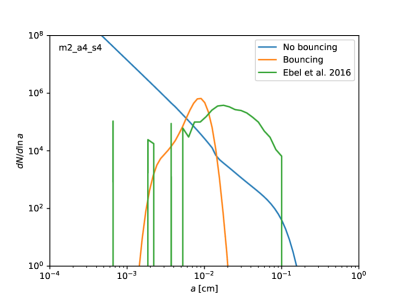
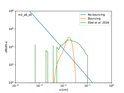
Figure 15: Logarithmic size distribution ($a\,dN/da=dN/\ln a$) of dust aggregates at $r=2.9\;\mathrm{au}$ in the protoplanetary disk. Left: Fiducial model m2_a4_s4. Right: Model m2_a6_s4, which is like the fiducial model but with a 100-times lower $\alpha$ value. The blue and orange curves are for the cases without a bouncing barrier and with a bouncing barrier, respectively, and they have been normalized such that $N=\int_{0}^{\infty}dN$ is the number of aggregates per square centimetre of the disk. The Ebel results are the chondrule radius distribution inferred from thin slices of Allende, shown with the green curve of their figure 7 (we note that we plot against the radius, while Ebel et al. (2016) plotted against the 2-log of the diameter). The normalization of the Ebel curve has been adjusted so that it equals that of the two other curves. We also note that due to the limited sample size, the renormalized Ebel curve is noise limited at about $dN/d\ln a\simeq 10^{4}$.

The bouncing barrier changes this situation in the following ways. First of all, we have shown that with an active bouncing barrier, a very narrow size distribution is obtained. A monodisperse size distribution is a reasonable approximation of this, and the modifications required for polydisperse or continuous size distributions may not be necessary. Second, the bouncing barrier reduces the typical size of the pebbles present in the disk, leading to a smaller Stokes number. That does not exclude the activation of the streaming instability, but it will slow it down by extending the growth times of the instability. Li & Youdin (2021) presented an extensive parameter study and found that the pre-clumping times typically grow by a factor of 100 when the Stokes number of the particle drops from 1 to 10^-2 or 10^-3. In some cases, for the lower Stokes numbers, no clumping is observed. Therefore, we concluded that the bouncing barrier will significantly affect the streaming instability by providing an essentially monodisperse size distribution and reduced Stokes numbers.

As for the efficiency of the pebble accretion scenario, we have shown in this paper that the bouncing barrier appears to prevent the formation of the very high pebble flux $\dot{M}_{\mathrm{d}}$ needed for the standard models of pebble accretion (see e.g., Bitsch et al., 2019). The presence of the bouncing barrier thus appears to be detrimental to planet formation. However, pebble accretion can also occur in dust traps or dust rings, where the efficiency does not depend on the pebble flux but on the pebble surface density (e.g., Jiang & Ormel, 2023). The effect of the bouncing barrier on the efficiency of planet formation may thus not be as simple as comparing the magnitude of the pebble flux.

5.6 Chondrule formation

The narrow size distribution of dust aggregates resulting from the bouncing barrier may have an interesting implication for chondritic meteorites. Chondrules are once-molten ”granules” (tiny spherical rocks) that make up a substantial fraction of the mass of chondritic meteorites. They have typical diameters between 0.1 and 1 millimeter, dependent on their chondrite group (Jones, 2012). A summary of measured size distributions of chondrules can be found in Friedrich et al. (2015). The formation mechanism of chondrules is still a matter of debate. The mystery lies in the fact that they are about 100$\cdots$1000 times larger and $10^{6\cdots 9}$ times more massive than interstellar dust grains, yet they are solid rocks instead of loosely bound dust aggregates. From petrological studies it can be inferred that during the first few million years of the Solar System, they must have undergone one or more ”flash heating” events (Jones, 1996), causing a dust aggregate to melt and form a tiny spherical rock that we today identify as a chondrule.

One possible chondrule formation mechanism is the passing of dust aggregates through the bow-shocks of planetary embryos on eccentric orbits (Morris et al., 2012). In this scenario, dust aggregates that freely float in the protoplanetary disk may have chance encounters with a planetary embryo that moves supersonically through the disk due to high eccentricity. The probability that the dust aggregate accretes onto the embryo is very low due to the small cross section of the embryo. But the probability of passing through the bow-shock induced by the embryo in the protoplanetary disk is much higher. In that case, the dust aggregate gets heated to temperatures above the liquidus and subsequently cools back to the background temperature to form a chondrule.

However, a key question is why the chondrules in meteorites are limited to a narrow size range between 0.1 and 1 millimeter. In terms of this scenario, this question translates into asking why the precursor dust aggregates have such a narrow size distribution. Turbulent size sorting has been cited and extensively modeled as a possible explanation (e.g., Cuzzi et al., 2001). That scenario, however, does not explain what happens to the de-selected dust aggregates. An alternative explanation was given by Jacquet (2014). He noted that the bouncing barrier has a very weak dependence on disk parameters, such as the turbulence parameter $\alpha$, leading to a rather model-independent maximum dust aggregate size and a narrow size distribution. If these dust aggregates are then flash heated, they produce the right kind of distributions of sizes for the resulting chondrules.

We found exactly this phenomenon happening in our models. As can be seen in Fig. 16, even for strongly varying $\alpha$, the typical sizes of the dust aggregates remain rather similar. Indeed, we already found this insensitivity in our analytic estimates of the bouncing barrier in Section 3.2, cf. Eq. (12). As we show in this paper, and as can also be seen in Estrada et al. (2016), the presence of the bouncing barrier produces a very narrow size distribution of dust aggregates. If only a certain fraction of these dust aggregates are flash heated, the remainder of the dust aggregates stay unmolten and are available to form the matrix of a chondrite in a planetesimal-forming event, such as those triggered by the streaming instability (Carrera et al., 2015).

To test this hypothesis, we compared the vertically integrated size distribution of our fiducial model (m2_a4_s4 and its no-bouncing sibling) at $r=2.9\;\mathrm{au}$ with the chondrule size distribution in the Allende family of chondritic meteorites. We used the size distribution determined by Ebel et al. (2016), as shown in the green curve of their Figure 7. They do not count matrix particles, but their results show a clear scarcity of particles with radii between $10^{-3}$ and $10^{-2}$ cm and a clear peak of the distribution at around a radius of 0.15 mm. The results of the comparison are shown in Fig. 15 (left).

It is evident that the model without the bouncing barrier (blue curve in Fig. 15) has a problem when compared to the chondrule statistics (the green curve). It predicts far too many small particles with sizes between monomers and 0.1 mm, and it does not have a peak at some typical size. However, it does have a cutoff radius very similar to that of the chondrules. The model with the bouncing barrier (the orange curve) also has problems. It is narrower than the chondrule statistics of Ebel et al., and it peaks at a too small radius (by about a factor of two).

In Fig. 15 (right) the same is shown but for a much lower turbulent strength: $\alpha=10^{-6}$. The model without the bouncing barrier in figure differs even more from the chondrule curve, and the model with the bouncing barrier peaks at the correct radius, yet it is still too narrow.

This comparison has to be interpreted with some care. The radii of the dust aggregate precursors of the chondrules are porous. In our model, we have a porosity of about 0.397, implying an increased radius for the same mass of about 15%, which is still small compared to the range of radii over which we compare the results. The porosity of the actual chondrule precursors may have been higher. Furthermore, other parameters, such as the disk mass and the monomer size, enter into the result as well. But overall, the rough size range seems to match, even though the observed size distribution is not quite as narrow as our calculations predict. The bouncing barrier therefore should be considered as a possible factor contributing to the size distribution of chondrules in meteorites.

6 Conclusions

We studied the effects of the bouncing barrier in global models of dust evolution in planet-forming disks. Through our work, we arrived at the following conclusions:

1. When the bouncing is implemented into a global dust evolution model, it introduces several important changes.

2. The dust size distribution becomes much narrower, with a standard deviation in the natural logarithm of only 0.2, compared to a formal width of 2.5 in a typical non-bouncing run. The dust is then present as a quasi-monodisperse size set by the bouncing barrier.

3. The efficient removal of small $\mu\mathrm{m}$-sized grains should be visible in scattered light images and mid-IR spectroscopy, and it might be diagnosed by them.

4. Nevertheless, the disk does not become vertically optically thin unless much dust is converted into planetesimals.

5. Both the mean and the maximum steady-state dust particle sizes change significantly when the bouncing barrier is activated. The amount of change depends on a number of parameters, such as the turbulence strength and the disk mass.

6. The bouncing barrier strongly dampens the effect of changing the disk mass. Without bouncing, an increase in disk mass leads to a larger pebble flux initially and then to a more rapid global dust depletion. Bouncing moderates both of these effects. The pebble flux increases only moderately, and the dust disk survives longer.

7. The effects of making the dust aggregates mechanically (for example by using a smaller monomer size, which in effect increases the fragmentation velocity) are also very much damped with bouncing.

8. In the presence of an active bouncing barrier, the streaming instability will likely not be polydisperse because of the quasi-monodisperse size distribution. The speed and the efficiency of the streaming instability will be modified, but details will depend on circumstances.

9. The narrow size distribution of chondrules found in individual meteorites may be related to the bouncing barrier because the bouncing barrier may set the population of dust aggregates that are chondrule precursors.

10. The universality of chondrule sizes across different meteorites could be caused by the insensitivity of the bouncing barrier to disk parameters, in line with what was suggested by Jacquet (2014).

The bouncing barrier, when effective, does change the course of the evolution of the dust component in a planet-forming disk. In particular, the barrier should be considered in models that heavily lean on streaming instability, particle concentration, and pebble accretion.

Appendix A Diagnostics

To analyze the results from the DustPy code, there were a number of aposteriori (i.e., after the model run) diagnostics we calculated. In this appendix, we give the definitions of these diagnostic quantities.

A.1 Mean and width of the size distribution

At each radius $r$, we computed the mean grain size

$$\langle a\rangle(r)=\frac{1}{\Sigma_{\mathrm{d}}(r)}\int_{m_{\mathrm{min}}}^{m_{\mathrm{max}}}\Sigma_{\mathrm{d}}(r,m)a(m)dm,$$ (17)

where $\Sigma_{\mathrm{d}}(r)$ is the total dust surface density

$$\Sigma_{\mathrm{d}}^{\mathrm{tot}}(r)=\int_{m_{\mathrm{min}}}^{m_{\mathrm{max}}}\Sigma_{\mathrm{d}}(r,m)dm,$$ (18)

and $a(m)$ is

$$a(m)=\left(\frac{3m}{4\pi\rho_{\bullet}}\right)^{1/3}.$$ (19)

Furthermore, we computed an indication a_max of the maximum grains size as the largest grain size where the $\Sigma_{\mathrm{d}}$ drops below $10^{-3}$ times the maximum value of $\Sigma_{\mathrm{d}}$ at that radius.

We also note that in the DustPy code, the Sigma of the dust is defined such that it is already multiplied by the mass bin width, dust.Sigma[i,n]$\equiv\Sigma_{\mathrm{d}}(r_{i},m_{n})\Delta m_{n}$, so that the integral of Eq. (18) is, in Python, just the sum dust.Sigma.sum(axis=-1).

The width of the distribution was computed as the standard deviation $\sigma^{2}_{\ln(a)}$ of $\ln(a)$ from the value $\ln(\langle a\rangle(r))$:

$$\sigma^{2}_{\ln(a)}=\frac{1}{\Sigma_{\mathrm{d}}(r)}\int_{m_{\mathrm{min}}}^{m_{\mathrm{max}}}\Sigma_{\mathrm{d}}(r,m)[\ln(a(m))-\ln(\langle a\rangle(r))]^{2}dm.$$ (20)

The reason we defined the width in natural-log space instead of in linear space is that for the models without the bouncing barrier, the size distribution becomes rather wide, spanning several orders of magnitude in grain radius $a$, which is difficult to capture in linear $a$ space. We used the natural log instead of the 10-log because in the limit of small values of the standard deviation $\sigma^{2}_{\ln(a)}$, this value becomes equal to the linear standard deviation divided by the mean squared,

$$\lim_{\sigma^{2}\rightarrow 0}\sigma^{2}_{\ln(a)}=\frac{\sigma^{2}_{a}}{\langle a\rangle^{2}},$$ (21)

which can be proven by employing a Taylor expansion. Hence, for $\sigma^{2}_{\ln(a)}\ll 1$, we can unambiguously state that the size distribution is narrow, while for $\sigma^{2}_{\ln(a)}\gtrsim 1$, it is wide.

A.2 Optical depth of the dust distribution

To compute the optical depth, we first needed to compute the opacities of the different grain sizes. We used optool (Dominik et al. 2021) with the DHS (distribution of hollow spheres) formalism (Min et al. 2005), setting the $f_{\mathrm{max}}$ parameter to 0.8. The mixture was 87% pyroxene, with 70% magnesium (Dorschner et al. 1995), and the other 13% was amorphous carbon (Zubko et al. 1996). The porosity was set to 0.397 so that the mean material density of the dust aggregates would be $\rho_{\bullet}=1.67$, consistent with the DustPy model. With these opacities, we could then compute the total vertical optical depth at wavelength $\lambda$ at location $r$:

$$\tau_{\lambda}(r)=\int_{m_{\mathrm{min}}}^{m_{\mathrm{max}}}\Sigma_{\mathrm{d}}(r,m)\kappa_{\nu}(m)\,dm.$$ (22)

A.3 Images of the disk

To make images of the disk that could be compared to observations, we used the RADMC-3D radiative transfer code (Dullemond et al. 2012). We made one image at $\lambda=1\mu$m at an inclination $i=70^{\circ}$ and another image at $\lambda=1.3$mm at an inclination $i=90^{\circ}$. By choosing $i=70^{\circ}$ for the $1\mu$m image, we could better see the shape of the surface layers, while by choosing $i=90^{\circ}$ for the 1.3 mm image, we could better see the vertical extent of the dust.

A.4 Degree of settling

DustPy stores the vertical extent $H_{\mathrm{d}}(r,m)$ of each grain mass and at each location. To obtain the mean dust vertical extent $H_{\mathrm{d}}(r)$ we computed

$$H^{\mathrm{tot}}_{\mathrm{d}}(r)=\frac{1}{\Sigma_{\mathrm{d}}(r)}\int_{m_{\mathrm{min}}}^{m_{\mathrm{max}}}H_{\mathrm{d}}(r,m)\Sigma_{\mathrm{d}}(r,m)dm.$$ (23)

A.5 Number of collisions per megayear

The bouncing barrier is thought to be accompanied or even triggered by collisional compaction (Zsom et al. 2010). Dust aggregates tend to initially grow in a ”fluffy” manner, often called ”fractal growth.” That is because each collision may lead to some degree of compactification but also to growth. At some point, the combination of slight compaction and increased velocities are then assumed to lead to the appearance of bouncing. From there, collisions no longer lead to growth, and the effect of further collisions can then successively compactify the aggregates. These aggregates remain porous, but they lose their fractal ”fluffy” shape. Being more round and compact to some degree, they tend to bounce even more (i.e., stick even less) to similar-sized aggregates. This reinforces the bouncing barrier, as is shown very clearly in Figure 4b of Zsom et al. (2010), where the ”enlargement factor” is reduced during bouncing, and Figure 4c, where the ”bouncing with compaction” dominates after the bouncing barrier has been reached. The compaction, however, requires some time, or better, it requires numerous successive collisions. Exact quantitative values of the required number of collisions are not known, but it is worthwhile to find out whether in the current model, the expected number of collisions is much larger than unity or not. Of course, our model does not include the effect of fractal growth, but if it did, it would likely increase the collision rate rather than decrease it, so our model can provide a lower limit to the number of collisions. If the result is that the number of collisions is much larger than unity, then we may expect the dust aggregates to have time to become nicely rounded-off and ”pebble-like.”

The simplest definition of the mean collision rate (the number of collisions per dust aggregate per second) is

$$R_{\mathrm{coll}}^{\mathrm{tot}}(m)=\int_{m_{\mathrm{min}}}^{m_{\mathrm{max}}}\sigma_{\mathrm{coll}}(m,m^{\prime})\,\Delta v(m,m^{\prime})\,n(m^{\prime})\,dm^{\prime},$$ (24)

where $\sigma_{\mathrm{coll}}(m,m^{\prime})=\pi(a+a^{\prime})^{2}$ (using Eq. 19) is the collisional cross section, $\Delta v(r,m,m^{\prime})$ is the expected relative collisional velocity, and $n(r,m^{\prime})=\Sigma_{\mathrm{d}}(r,m^{\prime})/(\sqrt{2\pi}h_{\mathrm{d}}(r,m^{\prime})m^{\prime})$ is the midplane volume number density of particles with mass $m^{\prime}$, where $h_{\mathrm{d}}(r,m^{\prime})$ is the vertical extent of the layer of these dust aggregates.

The problem with this definition of the number of collisions is that it includes collisions of a dust aggregate with any mass, including tiny (micron sized) dust particles. This means that for a millimeter size dust aggregate, it also includes collisions with micron-sized particles. This may lead to very large numbers, even if the number of collisions between similar-sized aggregates remains low. A better definition that accounts for the mass ratio of the particles is

$$R_{\mathrm{coll}}^{\mathrm{ratio}}(r,m)=\int\limits_{m_{\mathrm{min}}}^{m_{\mathrm{max}}}\sigma_{\mathrm{coll}}(m,m^{\prime})\,\Delta v(r,m,m^{\prime})\,\min\left(\frac{m^{\prime}}{m},1\right)\,n(r,m^{\prime})\,dm^{\prime},$$ (25)

where we scale the weight of collisions with very small collision partners with the mass ratio. Alternatively, we could simply limit ourselves to collisions with almost equal sized dust aggregates:

$$R_{\mathrm{coll}}^{\mathrm{equ}}(r,m)=\int_{m/2}^{2m}\sigma_{\mathrm{coll}}(r,m,m^{\prime})\,\Delta v(r,m,m^{\prime})\,n(r,m^{\prime})\,dm^{\prime}.$$ (26)

Next, for each of these definitions, we took the mean over mass:

$$\bar{R}_{\mathrm{coll}}^{\mathrm{X}}(r)=\frac{1}{\Sigma^{\mathrm{tot}}_{\mathrm{d}}(r)}\int_{m_{\mathrm{min}}}^{m_{\mathrm{max}}}\Sigma_{\mathrm{d}}(r,m)\,R_{\mathrm{coll}}^{\mathrm{X}}(r,m)\,dm,$$ (27)

where X is a placeholder for tot, ratio, or equ. We re-inserted the $r$-dependency here for clarity.

Finally, to use a more meaningful timescale, we estimated the number of collisions per megayear simply by multiplying by $3.15576\times 10^{13}$ seconds:

$$\bar{R}_{\mathrm{coll,Myr}}^{\mathrm{X}}(r)=3.15576\times 10^{13}\;\bar{R}_{\mathrm{coll}}^{\mathrm{X}}(r).$$ (28)

A.6 Mean collisional velocity

The mean collisional velocity was computed for ”almost equal size” collisions, as in Eq. (26). The integral becomes quadratic in $\Delta v(r,m,m^{\prime})$ because we need one factor $\Delta v$ for the collision rate and another factor $\Delta v$ for computing the mean:

$$\begin{split}\langle\Delta v_{\mathrm{coll}}^{\mathrm{equ}}(r)\rangle=&\bar{R}_{\mathrm{coll}}^{\mathrm{X}}(r)^{-1}\,\int_{m/2}^{2m}\int_{m/2}^{2m}\sigma_{\mathrm{coll}}(r,m,m^{\prime})\;\times\\ &\,\Delta v(r,m,m^{\prime})^{2}\,n(r,m^{\prime})\,n(r,m)\,dm^{\prime}dm.\end{split}$$ (29)

Appendix B Size distributions for the turbulence series and miscellaneous series

In Sections 4.3 and 4.4, the results for the two series of models were discussed. Here we show the full distribution function data.

Appendix C Resolution test

To ascertain that the mass resolution is sufficient to capture the narrow mass distributions we obtained with the bouncing barrier, we redid the fiducial model with twice the number of mass sampling points ($N_{m}=240$) and compared the distributions at $r=3.13$ au. As shown in Fig. 18, the result shows that while the distribution peak in the fiducial resolution model is slightly shifted with respect to the high resolution model, the overall match is satisfactory.

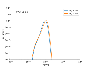
Figure 18: As in Fig. 4 but now the model with the fiducial mass resolution ($N_{m}=120$) is compared to a run with double the resolution ($N_{m}=240$).

To ascertain the correct choice of time steps for the integration, we made runs with different time step boost factors. The effects of this can be seen in many model outcomes. We chose the plot showing the collision velocities. The results are shown in fig. 19 and demonstrate that the results are very similar with boost factors of 1 and 10, but that the computation becomes unstable with a boost factor of 100.

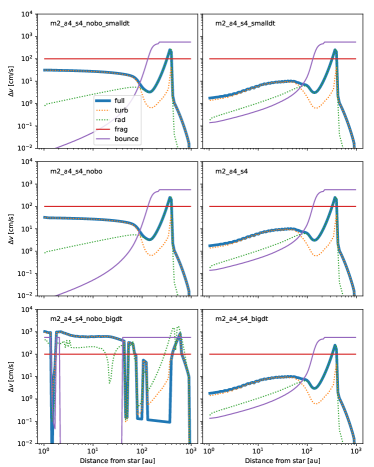
Figure 19: As in Fig. 5 but created from runs with different time steps with boosting factors 1, 10, and 100, from top to bottom.

Appendix D Code snippets for implementing the bouncing barrier into DustPy

To implement the bouncing barrier into DustPy, we first (before calling sim.run()) computed the bouncing velocity $v_{\mathrm{b}}$

⬇

sim.dust.froll = 1e-4 # Heim et al. 1999

sim.dust.mredu = sim.grid.m[:,None] * sim.grid.m[None,:] / ( sim.grid.m[:,None] + sim.grid.m[None,:] )

sim.dust.v.bounce = np.sqrt(5*np.pi*sim.dust.amono* sim.dust.froll/sim.dust.mredu) # Eq. 7 of Guettler et al. 2010

Next we overrode the sim.dust.p.stick() function of DustPy by defining our own

⬇

def dd_p_stick(sim):

dum = (sim.dust.v.bounce[None,:,:]/ sim.dust.v.rel.tot)**2

sim.dust.p.bounce = (1.5*dum + 1) * np.exp(-1.5*dum)

pnostick = np.maximum(sim.dust.p.frag, sim.dust.p.bounce)

p = 1. - pnostick

p[0] = 0.

p[-1] = 0.

return p

and we linked it in through the following assignment.

⬇

sim.dust.p.stick.updater = dd_p_stick

Appendix E Table of symbols

Here is a table of often-used symbols of this paper. The dimension column gives the dimension of the quantity. The last column gives the equation or section where the symbol first appears.
Symbol Meaning Dim Eq/Sec $t$ Time s $\sigma_{\mathrm{H}_{2}}$ Cross section of (H₂) collisions cm² Sec. 3.2 $\sigma_{\mathrm{coll}}$ Cross section dust prtcl collisions cm² Eq. 24 $\sigma_{\ln(a)}$ Width of size distribution - Eq. 20 $\Sigma_{\mathrm{g}}$ Gas surface density g cm^-2 Eq. 15 $\Sigma_{\mathrm{d}}^{\mathrm{tot}}$ Totad dust surface density g cm^-2 Eq. 18 $\mathrm{St}$ Stokes number grain size $a$ - Eq. 9 $\mathrm{St}_{\mathrm{b0}}$ St at bouncing barrier - Eq. 11 $\mathrm{St}_{\mathrm{f}}$ St at fragmentation barrier - Eq. 8 $a_{\mathrm{b0}}$ Size limit due to bouncing cm Eq. 12 $v_{\mathrm{stick}}$ Sticking velocity cm s^-1 Eq. 3 $v_{\mathrm{b}}$ Bouncing velocity cm s^-1 Eq. 5 $v_{\mathrm{f}}$ Fragmentation velocity cm s^-1 Eq. 2 $\sigma^{2}_{\ln(a)}$ Width of size distribution peak - Eq. 20 $\langle a\rangle$ Mean grain size cm Eq.17