FastPart: Over-Parameterized Stochastic Gradient Descent
for Sparse optimisation on Measures

Abstract

This paper presents a novel algorithm that leverages Stochastic Gradient Descent strategies in conjunction with Random Features to augment the scalability of Conic Particle Gradient Descent (CPGD) specifically tailored for solving sparse optimisation problems on measures. By formulating the CPGD steps within a variational framework, we provide rigorous mathematical proofs demonstrating the following key findings: $\mathrm{(i)}$ The total variation norms of the solution measures along the descent trajectory remain bounded, ensuring stability and preventing undesirable divergence; $\mathrm{(ii)}$ We establish a global convergence guarantee with a convergence rate of $\mathcal{O}(\log(K)/\sqrt{K})$ over $K$ iterations, showcasing the efficiency and effectiveness of our algorithm, $\mathrm{(iii)}$ Additionally, we analyze and establish local control over the first-order condition discrepancy, contributing to a deeper understanding of the algorithm’s behavior and reliability in practical applications.

1 Introduction

1.1 Convex programming for sparse optimisation on measures

Convex optimisation on the space of measures has gained attention during the past decade, e.g., Bach and Chizat (2021); Chizat and Bach (2018); Chizat (2022); De Castro et al. (2021); Poon et al. (2021); De Castro and Gamboa (2012); Candès and Fernandez-Granda (2014) and references therein. It is also a popular field of investigation to derive global optimisation methods (a.k.a. simulated annealing) through the embedding of $\mathds{R}^{d}$ into the space of measures (Bolte et al., 2023; Miclo, 2023).

At his core, it can be viewed as a fruitful way of expressing many non-convex signal processing and machine learning tasks into a convex one, where one searches for an element of a Hilbert space $\mathds{H}$ that can be described as a linear combination of a few, say $\bar{s}$, elements:

$$\bar{\bm{y}}=\sum_{j=1}^{\bar{s}}\bar{\omega}_{j}\varphi_{\bar{\bm{t}}_{j}}\,,$$ (1.1)

from a given parameterized set $\big{\{}\varphi_{\bm{t}}\,:\,{\bm{t}}\in\mathcal{X}\big{\}}$ where $\bar{\omega}_{j}\in\mathds{R}\setminus\{0\}$ and $\mathcal{X}$ a compact set of $\mathds{R}^{d}$.

Given an empirical observation ${\bm{y}}$, we would like to find a sparse representation, akin to (1.1), that explains ${\bm{y}}$ and for which the learnt parameters $(\omega_{j},{\bm{t}}_{j})_{j=1}^{s}$ encode an output solution for which generalization properties can be proven. A common practice is to minimize:

$$(\omega_{j},{\bm{t}}_{j})_{j=1}^{s}\mapsto\Big{\|}{\bm{y}}-\sum_{j=1}^{s}\omega_{j}\varphi_{{\bm{t}}_{j}}\Big{\|}^{2}_{\mathds{H}}\,,$$ (1.2)

which is a non-convex program. In the expression (1.2) above, $s\geq 1$ is a tuning parameter quantifying the so called sparsity of the solution.

A substantial body of literature pertains to the minimization of Mean Squared Error (MSE) and aligns with the framework outlined herein. In this paper, we will expound upon our methodology in a generalized format that can effectively encompass a majority of fields. Notably, certain specific instances will be elaborated upon within this paper, including but not limited to sparse deconvolution (De Castro and Gamboa, 2012; Candès and Fernandez-Granda, 2014), infinitely wide neural networks (Bach and Chizat, 2021; Chizat and Bach, 2018), or Mixture Models (De Castro et al., 2021). Our approach is deployed according to the following steps.

Lifting on the space of signed measures

First, we lift Program (1.2) onto the space $\mathcal{M}(\mathcal{X})$ of Radon measures with finite total variation norm on $\mathcal{X}$. Consider the positive definite kernel $\mathds{K}$ defined as the dot product $\mathds{K}({\bm{t}},{\bm{t}}^{\prime}):=\langle\varphi_{\bm{t}},\varphi_{{\bm{t}}^{\prime}}\rangle_{\mathds{H}}$ for all $t,t^{\prime}\in\mathcal{X}$, and assume that:

$$\text{the function }{\bm{t}}\in\mathcal{X}\mapsto\varphi_{\bm{t}}\in\mathds{H}\text{ is continuous}\,. \mathbf{A_{0}}$$ ()

Consider the kernel measure embedding (we refer to Appendix A.2 for further details),

$$\Phi:\ \nu\in\mathcal{M}(\mathcal{X})\mapsto\int_{\mathcal{X}}\varphi_{\bm{t}}\mathrm{d}\nu({\bm{t}})\in\mathds{H}\,.$$ (1.3)

It is proven in the appendix (see Lemma A.2) that $\Phi$ is a bounded linear map under ($\mathbf{A_{0}}$). We deduce that:

$$\nu\in\mathcal{M}(\mathcal{X})\mapsto\big{\|}{\bm{y}}-\Phi(\nu)\big{\|}^{2}_{\mathds{H}}\,,$$ (1.4)

is a convex function on $\mathcal{M}(\mathcal{X})$. Taking the set of discrete measures given by $\nu=\sum_{j=1}^{s}\omega_{j}\delta_{{\bm{t}}_{j}}$, where $\delta_{\bm{t}}$ is the Dirac mass at point ${\bm{t}}$, we uncover the parametrisation (1.2). Hence, we have lifted a non-convex program on $(\omega_{j},{\bm{t}}_{j})_{j=1}^{s}$ onto a convex program over a much larger space, the space of signed measures.

Total variation norm regularization

The second step is regularization. One key parameter is $s$, the number of learnt parameters, that should be considered to estimate (an approximation of) the true function (1.1). In practice, it can be cumbersome to tune this parameter and it might be better to resort to regularization. One benefit of the lifting on the space of measures is that this can be simply done by the $\mathrm{TV}$-norm. Inspired by $L^{1}$-regularization in (high-dimensional) inverse problems, we study the so-called Beurling LASSO (De Castro and Gamboa, 2012; Candès and Fernandez-Granda, 2014) referred to as BLASSO below, whose convex objective function is given by:

$$J(\nu):=\frac{1}{2}\big{\|}{\bm{y}}-\Phi(\nu)\big{\|}_{\mathds{H}}^{2}+\lambda\|\nu\|_{\mathrm{TV}}\,,$$ (1.5)

where $\lambda>0$ is a tuning parameter. We denote by $\mu^{\star}\in\mathcal{M}(\mathcal{X})$ a solution to BLASSO

$$J(\mu^{\star})=\min_{\mu\in\mathcal{M}(\mathcal{X})}J(\mu)\,. \mathcal{B}$$ ()

The existence of a solution to the problem at hand is not manifestly evident. Seminal contributions in the field, as articulated in (Bredies and Pikkarainen, 2013, Proposition 3.1) and (Hofmann et al., 2007, Theorem 3.1), have shown the existence of solutions upon continuity prerequisites imposed on the operator $\Phi$ or its pre-dual counterpart. Nevertheless, the arduousness associated with ascertaining the continuity and well-defined attributes of the operator $\Phi$ as expounded in Equation (1.3), within a given framework, underscores the complexity involved. In contrast, Condition ($\mathbf{A_{0}}$) affords a more tractable means of validation. Remarkably, our contribution lies in presenting a - to the best of our knowledge - novel result displayed in Theorem 1.1 below (established in Appendix A.3) that demonstrates the existence of solutions for any convex optimisation problem formulated in the manner of Equation (1.6), subject to the condition of continuity stipulated in Equation ($\mathbf{A_{0}}$).

Theorem 1.1.

Let $\mathds{H}$ be separable Hilbert space and let $\mathcal{X}$ be compact metric space. Consider the problem

$$\inf_{\mu\in\mathcal{M}(\mathcal{X})}\Big{\{}L(\Phi\mu)+\lambda\|\mu\|_{\mathrm{TV}}\Big{\}}$$ (1.6)

where $L\,:\,{\bm{h}}\in\mathds{H}\to L({\bm{h}})\in[0,\infty]$ is convex and lower semi-continuous. If ($\mathbf{A_{0}}$) holds then there exists a measure $\mu^{\star}\in\mathcal{M}(\mathcal{X})$ solution to (1.6). Furthermore, if $L$ is strictly convex, then the vector $\Phi(\mu^{\star})\in\mathds{H}$ is unique $($it does not depend on the choice of the solution $\mu^{\star})$.

Remark 1.1.

By choosing $L({\bm{h}})=(1/2)\|{\bm{y}}-{\bm{h}}\|_{\mathds{H}}^{2}$ in Theorem 1.1, it is established that there exists a signed measure $\mu^{\star}\in\mathcal{M}(\mathcal{X})$ solution to BLASSO ($\mathcal{B}$).

Over the last decade, several investigations on the performances of the estimator associated to the solution of (1.6) have been proposed in several specific situations. This solution can be proven to be close, for some partial Wasserstein $2$ distance (Poon et al., 2021), to the target measure $\bar{\mu}=\sum_{j=1}^{\bar{s}}\bar{\omega}_{j}\delta_{\bar{t}_{j}}$ involved in Equation (1.1) in some cases of interest $($e.g., Mixture Models (De Castro et al., 2021) or sparse deconvolution (Poon et al., 2021; De Castro and Gamboa, 2012)$\,)$ as soon as the support points ${\bar{t}_{j}}$ of the target $\bar{\mu}$ are sufficiently separated. Moreover, if the bounded linear map $\Phi$ has finite rank $m\geq 1$, then there exists a solution to ($\mathcal{B}$) with at most $m$ atoms, as proven by (Boyer et al., 2019, Section 4).

In this contribution, we focus our attention on the practical implementation of the optimisation problem ($\mathcal{B}$). In particular, our aim is to provide a runable and efficient algorithm, and to display associated theoretical guarantees.

1.2 Learning with over-parametrised non-convex objective functions

Solving ($\mathcal{B}$) from a practical point of view is not an immediate task, due to the infinite dimensional nature of the target. In this context, the Sliding Franck-Wolfe algorithm (see, e.g., Denoyelle et al. (2019)) provides an answer to this question. In this paper, we focus instead on the convergence of a Stochastic and Random Feature version of the Conic Particle Gradient Descent (CPGD) (Chizat, 2022) towards a minimum of Program ($\mathcal{B}$).

Writing the weights $\mathds{W}:=(\omega_{1},\ldots,\omega_{p})$ and the positions $\mathds{T}:=({\bm{t}}_{1},\ldots,{\bm{t}}_{p})\in\mathcal{X}^{p}$, we consider a generic measure with $p$ weighted particles by:

$$\nu(\mathds{W},\mathds{T}):=\sum_{j=1}^{p}\varepsilon_{j}\omega_{j}\delta_{{\bm{t}}_{j}},\,$$ (1.7)

where $\omega_{j}>0$ (resp. $\varepsilon_{j}=\pm 1$) refers to the weight (resp. the sign) of the particle $j$. The signs are fixed along the descent while the positions $\mathds{T}$ and weights $\mathds{W}$ are updated each gradient step. By a symmetrization argument, see for instance (Chizat, 2022, Appendix A), we consider, without loss of generality, that $\varepsilon=1$. It holds that minimizing ($\mathcal{B}$) or minimizing $J$ defined by:

$$J(\mu^{\star})=\min_{\mu\in\mathcal{M}(\mathcal{X})_{+}}J(\mu)\,. \mathcal{B}_{+}$$ ()

are equivalent, in a sense made precise by (Chizat, 2022, Proposition A.1) for instance; where $\mathcal{M}(\mathcal{X})_{+}$ is the set of nonnegative measures with finite $\mathrm{TV}$-norm. The attentive reader can uncover the next results on $\mathcal{M}(\mathcal{X})$ by replacing $\omega_{j}$ by $\varepsilon_{j}\omega_{j}$. The gradient descent dynamics are the same and our results also holds in this latter case.

Our algorithm makes use of particles measures as a proxy for solving the problem ($\mathcal{B}$). To this end, we adapt the notation of objective functions and related quantities accordingly. Denoting $\bm{\lambda}:=(\lambda,\ldots,\lambda)$, the definition of $\nu(\mathds{W},\mathds{T})$ in (1.7) then yields

$$J(\nu(\mathds{W},\mathds{T}))=\frac{1}{2}\Big{\|}{\bm{y}}-\sum_{j=1}^{p}\omega_{j}\varphi_{{\bm{t}}_{j}}\Big{\|}_{\mathds{H}}^{2}+\lambda\sum_{j=1}^{p}\omega_{j}:=F(\mathds{W},\mathds{T})+\frac{1}{2}\|{\bm{y}}\|_{\mathds{H}}^{2}\,,$$

where ${\bm{k}}_{\mathds{T}}:=(\langle{\bm{y}},\varphi_{{\bm{t}}_{1}}\rangle_{\mathds{H}},\ldots,\langle{\bm{y}},\varphi_{{\bm{t}}_{p}}\rangle_{\mathds{H}})\in\mathds{R}^{p}$, $\mathds{K}_{\mathds{T}}$ is a $(p\times p)$ matrix with entries $\mathds{K}({\bm{t}}_{i},{\bm{t}}_{j})$ defined by:

$$\mathds{K}({\bm{t}}_{i},{\bm{t}}_{j})=\langle\varphi_{{\bm{t}}_{i}},\varphi_{{\bm{t}}_{j}}\rangle_{\mathds{H}},$$ (1.8)

and

$$F(\mathds{W},\mathds{T}):=\langle\bm{\lambda}-{\bm{k}}_{\mathds{T}},\mathds{W}\rangle+\frac{1}{2}\mathds{W}^{T}\mathds{K}_{\mathds{T}}\mathds{W}\,,$$ (1.9)

is equal to $J(\nu(\mathds{W},\mathds{T}))$ up to the additive constant term $(1/2)\|{\bm{y}}\|_{\mathds{H}}^{2}$ (that only depends on the observations and not on the parameters of the measure we are optimising on).

In contrast to the original problem presented in ($\mathcal{B}$), the optimisation process now operates within a different domain. Instead of working within the space of measures $\mathcal{M}(\mathcal{X})$ (or $\mathcal{M}(\mathcal{X})_{+}$), it focuses on particle measures with a set of fixed size $p$. This shift in perspective involves optimising over both the positions $\mathds{T}$ and weights $\mathds{W}$. Although this adjustment serves to simplify the model’s complexity to some extent, it introduces certain computational challenges. Firstly, for each pair of parameters $(\mathds{W},\mathds{T})$, the computation of $F(\mathds{W},\mathds{T})$ necessitates the evaluation of ${\bm{k}}_{\bm{t}}$ and $\mathds{K}_{\mathds{T}}$. Depending on the structure of the Hilbert space $\mathds{H}$ and the associated scalar products, this computation can be time-consuming. The need to calculate these quantities at each iteration of a gradient descent algorithm can become problematic, especially when dealing with high-dimensional spaces ($d$ being significant). Furthermore, considering a large number of particles during the optimisation process, which is often essential, can substantially escalate the computational burden. This computational overhead needs to be carefully managed and optimised to ensure the efficiency of the optimisation procedure. In this paper, we address these issues by presenting a novel algorithm that incorporates Stochastic Gradient Descent (SGD) iterations. To the best of our knowledge, this approach has not been previously explored in the context of sparse optimisation within the domain of measures. We rigorously examine the properties of this algorithm, conducting a comprehensive investigation from both theoretical and practical perspectives.

The paper is organised as follows. First, we describe in Section 2 the construction of the algorithm and related necessary assumptions. Section 3 is illustrated by the example of deconvolution for mixture models, an important topic in unsupervised learning. Some theoretical results describing the behaviour of the algorithm in terms of the number of iterations are presented in Section 4, while a numerical illustration on some toy examples are discussed in Section 5. Proofs and related technical results are gathered in Section 6 and in Appendices A, B and C.

2 Construction of a Stochastic Gradient Descent algorithm.

The primary objective of this contribution is to introduce a stochastic algorithm designed for tackling the optimisation Program ($\mathcal{B}$), followed by an exploration of its underlying theoretical properties. Our approach initially stems from a deterministic algorithm, which is subsequently adapted into a stochastic variant to enhance computational efficiency. Considering Program ($\mathcal{B}$) as an optimisation challenge, it can be effectively addressed through the application of gradient descent (GD) techniques within the domain of measures. A straightforward algorithm would entail performing a discretized gradient descent on the space of non-negative measures $\mathcal{M}(\mathcal{X})_{+}$. However, in the absence of a significant conceptual breakthrough pertaining to an efficient parameterization of the preceding iteration within $\mathcal{M}(\mathcal{X})_{+}$ (or its dual spaces and Hilbert basis), we resort to emulating this gradient descent process through a collection of measures encoded with particles. This method of approximating optimisation over measures through particles finds its conceptual foundation in swarm optimisation approaches, as exemplified in recent works such as those of Bolte et al. (2023); Miclo (2023).

2.1 Mirror principled conic gradient descent

2.1.1 The Mirror descent principle

We first introduce a basic ingredient related to optimisation problems on geometric spaces, that permits to adapt the evolution of an algorithm to some constrained sets where the problem is embedded, without using some non-smooth additional projection steps. Mirror Descent (MD below) originates from the pioneering work of Nemirovskij and Yudin (1983) and permits to naturally handle optimisation problems especially when the mirror/proximal mapping is explicit, which is indeed the case for a convex problem constrained on measures as $\mathcal{M}(\mathcal{X})_{+}$ (see e.g. Lan et al. (2012), Bubeck et al. (2015)).

The MD approach has the nice feature to define a smooth evolution that lives inside the constrained set without adding some supplementary projection step and “pushes” the frontiers of $\mathcal{M}(\mathcal{X})_{+}$ at an infinite distance from any point that lies strictly inside.

Consider a strongly convex function $h$ on $\mathds{R}_{+}^{p}\times\mathcal{X}^{p}$, we define the Bregman divergence associated to $h$ as follows: for two pairs $(\mathds{W}_{1},\mathds{T}_{1})$ and $(\mathds{W}_{2},\mathds{T}_{2})$ in $\mathds{R}_{+}^{p}\times\mathcal{X}^{p}$, we denote:

$$D_{h}((\mathds{W}_{1},\mathds{T}_{1}),(\mathds{W}_{2},\mathds{T}_{2}))=h(\mathds{W}_{1},\mathds{T}_{1})-h(\mathds{W}_{2},\mathds{T}_{2})-\langle\nabla h(\mathds{W}_{2},\mathds{T}_{2}),(\mathds{W}_{1},\mathds{T}_{1})-(\mathds{W}_{2},\mathds{T}_{2})\rangle\,.$$ (2.1)

The Bregman divergence $D_{h}$ is then used to define the MD with the following variational characterisation

$$(\mathds{W}^{k+1},\mathds{T}^{k+1})=\arg\min_{(\mathds{W},\mathds{T})}\Big{\{}\big{\langle}\nabla F(\mathds{W}^{k},\mathds{T}^{k}),(\mathds{W},\mathds{T})-(\mathds{W}^{k},\mathds{T}^{k})\big{\rangle}+\frac{1}{\kappa}D_{h}\left((\mathds{W},\mathds{T}),(\mathds{W}^{k+1},\mathds{T}^{k+1})\right)\Big{\}}\,,$$ (2.2)

where $\kappa>0$ is the gradient step size.

2.1.2 A conic descent

In this contribution, we will consider the entropy function $\mathrm{Ent}$ on $\{\mathds{R}_{+}\}^{p}$ as:

$$\mathrm{Ent}(\mathds{W}):=\sum_{j=1}^{p}\omega_{j}\log(\omega_{j})$$ (2.3)

It induces the Bregman divergence defined on the set of positive weights as

$$D_{\mathrm{Ent}}(\mathds{W}^{1},\mathds{W}^{2})=\sum_{j=1}^{p}\omega^{1}_{j}\Bigg{(}\frac{\omega^{2}_{j}}{\omega^{1}_{j}}-1-\log\frac{\omega^{2}_{j}}{\omega^{1}_{j}}\Bigg{)}\,.$$ (2.4)

We then define the global divergence on the set $\mathds{R}_{+}^{p}\times\mathcal{X}^{p}$, as

$$\Delta_{\alpha,\eta}((\mathds{W}^{1},\mathds{T}^{1}),(\mathds{W}^{2},\mathds{T}^{2})) :=\frac{1}{\alpha}D_{\mathrm{Ent}}(\mathds{W}^{1},\mathds{W}^{2})+\frac{1}{\eta}D_{\mathrm{Conic}}((\mathds{W}^{1},\mathds{T}^{1}),(\mathds{W}^{2},\mathds{T}^{2}))\,,$$ (2.5)

$$\text{where }D_{\mathrm{Conic}}((\mathds{W}^{1},\mathds{T}^{1}),(\mathds{W}^{2},\mathds{T}^{2})) :=\sum_{j=1}^{p}\omega^{1}_{j}\|{\bm{t}}^{1}_{j}-{\bm{t}}^{2}_{j}\|^{2}\,.$$ (2.6)

In Equation (2.5) above, the parameter $\alpha>0$ is the gradient step size for the weights update and $\eta>0$ for the positions updates. This global divergence $\Delta_{\alpha,\eta}$ is used to compute the gradient descent updates thanks to the variational formulation (2.2). We incorporate the term $D_{\mathrm{Conic}}$ with the specific intention of aligning it with the gradient updates associated with Conic Particle Gradient Descent (CPGD), as presented for instance by (Chizat, 2022, Section 2.2).

Remark 2.1 (The conic metric…).

We recall that in the CPGD framework (Chizat, 2022, Section 2.2), the set of particles $(\omega,{\bm{t}})\in\mathds{R}_{+}\times\mathcal{X}$ is equipped with the Riemannian metric defined by $(1/2)\nabla_{\omega}^{2}+(\omega/2)\|\nabla_{\bm{t}}\|^{2}$ where $(\nabla_{\omega},\nabla_{\bm{t}})\in\mathbb{R}\times T_{(\omega,{\bm{t}})}(\mathcal{X})$ is a tangent vector at point $(\omega,{\bm{t}})$. As displayed below, we recognize a “conic” metric where two given fixed points ${\bm{t}}_{1},{\bm{t}}_{2}$ of $\mathcal{X}$ gets linearly closer as $\sqrt{\omega}$ goes to zero.

Then a mirror retraction is applied to $\omega$ (see Chizat (2022)[Definition 2.3]), corresponding to the Bregman divergence term $D_{\mathrm{Ent}}$ in our variational formulation. We notice that the term $D_{\mathrm{Conic}}$ comes from the latter conic metric.

Remark 2.2..is not a Bregman divergence..

It is noteworthy that $D_{\mathrm{Conic}}$ does not conform to the definition of a Bregman divergence, as outlined in Definition (2.1). Specifically, there exists no global function $h$ such that $D_{\mathrm{Conic}}$ can be expressed in the form of $D_{h}$. This is evident, for instance, by considering the boundedness of Bregman balls, a property that is conspicuously absent in the case of $D_{\mathrm{Conic}}$. Furthermore, a direct proof of this assertion can be established through a contradiction argument. If such a function $h$ were to exist for $p=1$, it would imply the following relationship

$$h(\omega_{1},{\bm{t}}_{1})-h(\omega_{2},{\bm{t}}_{2})-\langle\nabla h(\omega_{2},t_{2}),(\omega_{1}-\omega_{2},{\bm{t}}_{1}-{\bm{t}}_{2}))=\omega_{1}\|{\bm{t}}_{1}-{\bm{t}}_{2}\|^{2}\,.$$

Then, consider ${\bm{t}}_{2}=0$ and observe that necessarily $h(\omega_{1},{\bm{t}}_{1})=h(0,0)+\omega_{1}\|t_{1}\|^{2}$, by removing the linear part that is necessarily vanishing. Subsequent straightforward calculations would lead to a contradiction, thereby confirming the incompatibility of $D_{\mathrm{Conic}}$ with the Bregman divergence framework.

According to the above remark, our descent algorithm should rather be understood as a Riemannian (stochastic) gradient descent instead of a purely mirror descent. We will keep the MD abuse of terms in what follows as it refers essentially to the evolution of the weights and since it is the commonly used term in machine learning with exponentially parameterized weights. Nevertheless, the difference between $\Delta_{\alpha,\eta}$ and a Bregman divergence prevents the use of standard arguments of convergence for mirror descent algorithm.

2.2 Evaluation of the gradient and construction of a stochastic approximation

2.2.1 Algorithmic issues

Iterative algorithms based on (2.2) and (2.5) have already been at the core of theoretical investigations. We refer for instance to Chizat (2022) among others. The latter investigates an algorithm that requires some frequent calls to the gradient $\nabla F$ of the objective $F$ defined in (1.9). This gradient can be related to the Fréchet differential function ${\bm{t}}\mapsto J^{\prime}_{\nu}({\bm{t}})$ of $J(.)$ at point $\nu\in\mathcal{M}(\mathcal{X})_{+}$ and its gradient $\nabla_{\bm{t}}J^{\prime}_{\nu}$. The Fréchet differential $J^{\prime}_{\nu}$ is defined through the following first order Taylor expansion:

$$\forall\nu\in\mathcal{M}(\mathcal{X})_{+},\quad\nu+\sigma\in\mathcal{M}(\mathcal{X})_{+}\qquad J(\nu+\sigma)-J(\nu)=\langle J^{\prime}_{\nu},\sigma\rangle_{\mathcal{M}(\mathcal{X})^{\star},\mathcal{M}(\mathcal{X})}+q(\sigma)\,,$$ (2.7)

where $J^{\prime}_{\nu}$ is the Fréchet gradient and $q$ is a second order term. We refer to Proposition B.1 for details. According to Proposition B.3, for any ${\bm{t}}\in\mathcal{X}$, we have by Equation (B.3) that, given $\nu=\sum_{j=1}^{p}\omega_{j}\delta_{\bm{t}_{j}}$,

$$J^{\prime}_{\nu}({\bm{t}})=\sum_{j=1}^{p}\omega_{j}\langle\varphi_{\bm{t}},\varphi_{{\bm{t}}_{j}}\rangle_{\mathds{H}}-\langle\varphi_{\bm{t}},\bm{y}\rangle_{\mathds{H}}+\lambda\,.$$ (2.8)

The computation of these functions is time-consuming for the three reasons listed below. For each of these challenges, we outline our strategy to address them, and we introduce three notation—namely, the three random variables $U$, $V$, and $T$—which will be elaborated upon in the subsequent section. In Section 3.1, we will provide a concrete example illustrating this phenomenon.

Kernel evaluation: random variable $U$ for Random Fourier feature strategy

Firstly, it is important to note that these functions may necessitate integral approximations due to their lack of closed-form expressions. For instance, the computation of $J^{\prime}_{\nu}({\bm{t}})$ within each iteration of a gradient descent algorithm involves multiple evaluations of the kernel $\mathds{K}({\bm{t}},{\bm{t}}^{\prime})$, where $\mathds{K}({\bm{t}},{\bm{t}}^{\prime})$ is defined in Equation (1.8). In many cases, these evaluations rely on non-explicit integrals, posing computational challenges.

To circumvent this issue, we will employ a Random Fourier feature strategy. This strategy aims to approximate the kernel $\mathds{K}$ by using a low-rank random kernel, achieved by evaluating the integral defining the kernel through independent Monte Carlo sampling.

Large samples: random variable $V$ for picking a data sample at random

A second strategy is to employ stochastic gradient computation with batch sub-sampling, which entails selecting a single data point at random - a fundamental component of various stochastic algorithms. Within our framework, this can be realized by utilizing the observation vector ${\bm{y}}$. It is worth emphasizing that in specific scenarios, the observed signal $\bm{y}$ can itself be a random variable. For instance, consider the case where ${\bm{y}}:=\Psi_{N}({\bm{X}})$, with $\Psi_{N}:\,\mathds{R}^{N}\to\mathds{H}$ representing a bounded linear mapping and ${\bm{X}}=(x_{1},\ldots,x_{N})$ consisting of $N$ i.i.d. samples drawn from a probability measure $\rho$.

In such cases, it becomes feasible to generate an unbiased stochastic version of ${\bm{y}}$ by randomly selecting a single or a mini-batch data sample. Moreover, even if ${\bm{y}}$ is deterministic or does not match the aforementioned identity ${\bm{y}}:=\Psi_{N}({\bm{X}})$, it is always possible to employ a similar strategy as described above (Random Fourier feature) to approximate $\langle\varphi_{\bm{t}},{{\bm{y}}}\rangle_{\mathds{H}}$ itself. Certainly, note that the unbiased stochastic version of ${\bm{y}}$ and the low-rank random kernel approximation of $\langle\varphi_{\bm{t}},{{\bm{y}}}\rangle_{\mathds{H}}$ should be jointly considered whenever possible.

Many particles: random variable $T$ for picking a particle at random

The necessity for a large number of particles to attain convergence guarantees increases exponentially with the dimension $d$ of $\mathcal{X}$. Consequently, it may become impractical to update all particles during each gradient step.

As a final ingredient, we opt to update the weight and position of a particle or a mini-batch of particles, selected randomly, as a mean to mitigate this challenge.

2.2.2 Stochastic approximation of the gradient

We provide in this paragraph a general framework allowing the construction of the stochastic conic gradient particle algorithm we are studying. Specific examples are discussed in Section 3 below.

The formulation of a stochastic approximation for the gradient $\nabla F$ necessitates certain general assumptions, which are outlined below. Of particular significance is the introduction of a random variable $Z=(T,U,V)$, which serves as a way to alleviate the computational complexity associated with evaluating the variational formulation of the gradient descent step (2.2).

Assumption ($\mathbf{A_{1}}$). There exists a pair of random variables $(U,V)$ $($not necessarily independent$)$ such that, for any ${\bm{t}},{\bm{t}}^{\prime}\in\mathcal{X}$,

$$\langle\varphi_{{\bm{t}}},\varphi_{{\bm{t}}^{\prime}}\rangle_{\mathds{H}}=\mathds{E}_{U}{\bm{g}}_{{\bm{t}},{\bm{t}}^{\prime}}(U)\quad\mathrm{and}\quad\langle\varphi_{\bm{t}},{\bm{y}}\rangle_{\mathds{H}}=\mathbb{E}_{V}{\bm{h}}_{\bm{t}}(V)\,, \mathbf{A_{1}}$$ ()

for some explicit bounded functions ${\bm{g}}$ and ${\bm{h}}$.

The latter assumption allows for a stochastic approximation of the functional $J^{\prime}_{\nu}$. It exactly corresponds to what happens in Equation (3.11) below for the mixture model. Indeed, if we define a random variable $T$ with distribution $\nu/\nu(\mathcal{X})$ (assumed non-negative w.l.o.g as discussed in (1.7)), sampled independently from $(U,V)$, we then introduce:

$${\bm{J}}^{\prime}_{\nu}({\bm{t}},Z):=\|\nu\|_{\mathrm{TV}}\,{\bm{g}}_{{\bm{t}},T}(U)-{\bm{h}}_{\bm{t}}(V)+\lambda\quad\mathrm{where}\quad Z:=(T,U,V)\,.$$ (2.9)

According to ($\mathbf{A_{1}}$), we can write that

$${\bm{J}}^{\prime}_{\nu}({\bm{t}},Z):=J^{\prime}_{\nu}({\bm{t}})+\xi_{\nu}({\bm{t}},Z)\quad\mathrm{with}\quad\mathbb{E}_{Z}\xi_{\nu}({\bm{t}},Z)=0\quad\forall{\bm{t}}\in\mathcal{X}\,.$$ (2.10)

We can construct a similar stochastic approximation for the gradient (w.r.t. the position parameter) of the functional $J^{\prime}_{\nu}$. First remark that

$$\nabla_{\bm{t}}J^{\prime}_{\nu}({\bm{t}})=\sum_{j=1}^{p}\omega_{j}\nabla_{\bm{t}}\langle\varphi_{\bm{t}},\varphi_{{\bm{t}}_{j}}\rangle_{\mathds{H}}-\nabla_{\bm{t}}\langle\varphi_{\bm{t}},{\bm{y}}\rangle_{\mathds{H}}\,.$$

The following assumption allows the commutativity between derivation and expectation and is satisfied in many situations, including batch or mini-batch strategies and smooth integral computations. The associated term in the mixture model is (3.12) and its stochastic counterpart is (3.15).

Assumption ($\mathbf{A_{2}}$). The couple $(U,V)$ and the functions ${\bm{g}},{\bm{h}}$ introduced in Assumption ($\mathbf{A_{1}}$) satisfy

$$\nabla_{\bm{t}}\mathds{E}_{U}{\bm{g}}_{{\bm{t}},{\bm{t}}^{\prime}}(U)=\mathds{E}_{U}\nabla_{t}{\bm{g}}_{{\bm{t}},{\bm{t}}^{\prime}}(U)\quad\mathrm{and}\quad\nabla_{\bm{t}}\mathbb{E}_{V}{\bm{h}}_{\bm{t}}(V)=\mathbb{E}_{V}\nabla_{\bm{t}}{\bm{h}}_{\bm{t}}(V)\,, \mathbf{A_{2}}$$ ()

for any ${\bm{t}},{\bm{t}}^{\prime}\in\mathcal{X}$ and $\bm{g}$ and $\bm{h}$ have bounded derivatives.

Then, introduce

$${\bm{D}}_{\nu}({\bm{t}},Z):=\|\nu\|_{\mathrm{TV}}\,\nabla_{\bm{t}}{\bm{g}}_{{\bm{t}},T}(U)-\nabla_{\bm{t}}{\bm{h}}_{\bm{t}}(V)\,,$$ (2.11)

where $Z=(T,U,V)$ still denotes the same variable as above. We can then observe that

$${\bm{D}}_{\nu}({\bm{t}},Z):=\nabla_{\bm{t}}J^{\prime}_{\nu}({\bm{t}})+\zeta_{\nu}({\bm{t}},Z)\quad\mathrm{with}\quad\mathbb{E}_{Z}\zeta_{\nu}({\bm{t}},Z)=0\quad\forall{\bm{t}}\in\mathcal{X}\,,$$ (2.12)

where we have used Assumptions ($\mathbf{A_{1}}$) and ($\mathbf{A_{2}}$).

Lemma B.1 provides a concrete and uniform upper bound on $J^{\prime}_{\nu}$ for any $\nu\in\mathcal{M}(\mathcal{X})_{+}$. From this remark, the boundedness of the functions ${\bm{g}}$ and ${\bm{f}}$ is indeed a reasonable assumption within this context.

Furthermore, in addition to the conclusions presented in Equations (2.10) and (2.12), that establish unbiased estimations of $J^{\prime}_{\nu}$ and $\nabla_{\bm{t}}J^{\prime}_{\nu}$, it is imperative to highlight that our assumptions ($\mathbf{A_{1}}$) and ($\mathbf{A_{2}}$) also result in almost sure upper bounds on $|J_{\nu}^{\prime}(.,Z)|$ and $\|D_{\nu}(.,Z)\|$ (for more comprehensive details, we refer to Lemma B.1 and Proposition C.1 ).

Algorithm 1 Stochastic & Random Feature Conic Particle Gradient Descent (FastPart)

1:Constant learning rates $(\alpha,\eta)$, Initialization $(\mathds{W}^{0},\mathds{T}^{0})$; $\triangleright$ Weights: $\mathds{W}^{k}$ and Positions: $\mathds{T}^{k}$

2:for $k=1,\ldots,K$  do$\triangleright$ $K$ gradient steps

3:     Set $\nu_{k}\longleftarrow\nu(\mathds{W}^{k},\mathds{T}^{k})$;$\triangleright$ Particles

4:     Sample $Z^{k+1}\longleftarrow(T^{k+1},U^{k+1},V^{k+1})$;$\triangleright$ Stochastic variables

5:     Compute ${\bm{J}}^{\prime}_{\nu_{k}}(\mathds{T}^{k},Z^{k+1})$ as defined by (2.9);$\triangleright$ Stochastic weights gradient

6:     Compute ${\bm{D}}_{\nu_{k}}(\mathds{T}^{k},Z^{k+1})$ as defined by (2.11);$\triangleright$ Stochastic positions gradient

7:     Compute

$$d^{k+1}\longleftarrow({\bm{J}}^{\prime}_{\nu_{k}}(\mathds{T}^{k},Z^{k+1}),\mathds{W}^{k}\odot{\bm{D}}_{\nu_{k}}(\mathds{T}^{k},Z^{k+1}))$$

where $u\odot v$ denotes the vector $(u_{i}v_{i})_{i}$;$\triangleright$ Stochastic Conic Particle Gradient (see Proposition B.3)

8:     Update the weights and positions with

$$(\mathds{W}^{k+1},\mathds{T}^{k+1}):=\arg\min_{(\mathds{W},\mathds{T})}\langle d^{k+1},(\mathds{W},\mathds{T})-(\mathds{W}^{k},\mathds{T}^{k})\rangle+\Delta_{\alpha,\eta}\left((\mathds{W},\mathds{T}),(\mathds{W}^{k},\mathds{T}^{k})\right)\,,$$ (2.13)

with $\Delta_{\alpha,\eta}$ given by (2.5).$\triangleright$ Mirror descent

9:end for

2.2.3 Stochastic conic particle gradient descent (FastPart)

With all these essential components in place, we are now prepared to construct our algorithm. The fundamental concept behind this approach is to substitute the deterministic gradient $\nabla F$ of $F$ in the mirror descent (2.2) with its stochastic counterpart, as derived from the stochastic gradients on weights (2.9) and positions (2.11) under Assumptions ($\mathbf{A_{1}}$) and ($\mathbf{A_{2}}$). In Algorithm 1, we introduce our stochastic optimisation method. This algorithm is defined through the utilization of stochastic, unbiased realizations, as outlined in the preceding assumptions.

Mirror descent updates

An important remark for the tractability of the Stochastic CPGD is that Equation (2.13) may be made explicit and simply corresponds to the following updates of the weights:

$$\forall j\in\{1,\ldots,p\}\,,\qquad\omega^{k+1}_{j}=\omega^{k}_{j}e^{-\alpha{\bm{J}}^{\prime}_{\nu_{k}}({\bm{t}}^{k}_{j},Z^{k+1})}\,.$$ (2.14)

In a similar way, it may be verified that the positions are updated as follows:

$$\mathds{T}^{k+1}=\mathds{T}^{k}-\eta{\bm{D}}_{\nu_{k}}(\mathds{T}^{k},Z^{k+1})$$ (2.15)

Properties

In what follows, we will study the properties of Algorithm 1 when the number $K$ of iterations becomes large, and will establish some convergence and reconstruction properties when the several parameters involved in the method are correctly tuned (learning rates $\alpha$ and $\eta$, number of particles $p$, and number of iterations $K$).

3 Some examples from Unsupervised learning and Signal processing

3.1 Mixture Models (M.M.)

3.1.1 Introduction

For the sake of clarity, we discuss briefly in this section the specific case of statistical mixture models. They are a class of statistical models that can be used for various purposes such as inference, testing, and modeling, have garnered significant attention in recent years due to their versatility and simplicity. However, the estimation of mixture models remains a complex task, with many aspects of the process not yet fully understood. The Expectation-Maximization (E.M.) algorithm, introduced by Dempster et al. (1977), and its subsequent generalization to stochastic variants in Delyon et al. (1999), have played a crucial role in the development of M.M.. Notably, the E.M. algorithm has been reinterpreted on exponential families as a descent algorithm with a surrogate in Kunstner et al. (2021), which has led to a renewed interest in M.M. within the machine learning and optimisation communities. Our work is also related to preliminary experiments conducted in De Castro et al. (2021), which employed a deterministic version of particle gradient descent. These experiments demonstrated the potential of using such methods in the context of M.M., and have inspired further research in this area. While M.M. may appear straightforward at first glance, their estimation poses significant challenges. However, recent advances in the field, including the reinterpretation of the EM algorithm and the use of descent algorithms with surrogates, have reignited interest in these models and their potential applications.

In this setting, the data ${\bm{X}}=(x_{1},\dots,x_{N})$ are i.i.d. random variables having a density $\rho$ in $\mathds{R}^{d}$ (w.r.t. the Lebesgue measure) verifying:

$$\rho=\theta\star\bar{\mu}=\sum_{j=1}^{\bar{s}}{\bar{\omega}}_{j}\theta_{\bar{\bm{t}}_{j}}\text{ with }\bar{\mu}:=\sum_{j=1}^{\bar{s}}{\bar{\omega}}_{j}\delta_{\bar{\bm{t}}_{j}}\,,$$

where $\bar{\mu}$ is an unknown mixing distribution, $\theta$ is a known even density on $\mathds{R}^{d}$ and $\theta_{\bm{t}}(\cdot)=\theta({\bm{t}}-\cdot)$. In the expression above, the symbol $\star$ denotes the convolution product. The goal in this context is to recover the target $\bar{\mu}$ and/or the corresponding weights $\overline{\mathds{W}}:=(\bar{\omega}_{1},\ldots,\bar{\omega}_{\bar{s}})$ and positions $\overline{\mathds{T}}:=(\bar{\bm{t}}_{1},\ldots,\bar{\bm{t}}_{\bar{s}})$.

3.1.2 Model specification

Following De Castro et al. (2021), we consider the Hilbert space $\mathds{H}$ defined as the RKHS associated to the $\mathrm{sinc}_{m}$ kernel, denoted by $\gamma_{m}$, for some bandwidth parameter $m$ and leading to

$$\mathds{H}:=\Big{\{}f:\mathds{R}^{d}\rightarrow\mathds{R}\ :\ \|f\|_{\mathds{H}}^{2}=\int_{\mathds{R}^{d}}\frac{|\mathcal{F}[f]({\bm{t}})|^{2}}{\mathcal{F}[\gamma_{m}]({\bm{t}})}\mathrm{d}{\bm{t}}<+\infty\Big{\}}\quad\text{with}\quad{\mathcal{F}[\gamma_{m}]}=\mathbf{1}_{[-m;m]^{d}}\,,$$

where $\mathcal{F}$ is the Fourier transform defined as

$$\forall s\in\mathds{R}^{d}\,,\quad\forall f\in\mathds{H}\,,\qquad\mathcal{F}[f]({\bm{s}}):=\int_{\mathds{R}^{d}}f({\bm{t}})e^{-\mathfrak{i}\langle{\bm{s}},{\bm{t}}\rangle}\mathrm{d}{\bm{t}},$$

and $\mathfrak{i}$ refers to the complex number. The inner product associated to the space $\mathds{H}$ hence verifies

$$\forall f,g\in\mathds{H}\,,\qquad\langle f,g\rangle_{\mathds{H}}=\mathcal{R}\Big{(}\int_{[-m;m]^{d}}\mathcal{F}[f]({\bm{t}})\times\overline{\mathcal{F}[g]({\bm{t}})}\mathrm{d}{\bm{t}}\Big{)}\,,$$ (3.1)

where $\mathcal{R}(z)$ denotes the real part of a complex number $z$. As in De Castro et al. (2021), we embed the sample ${\bm{X}}$ and the density $\rho$ in the same Hilbert space $\mathds{H}$ taking a convolution by the $\mathrm{sinc}_{m}$ kernel. It yields

$${\bm{y}}=\Psi_{N}({\bm{X}}):=\frac{1}{N}\sum_{i=1}^{N}\gamma_{m}(x_{i}-\cdot)\text{ and }\bar{\bm{y}}:=\mathds{E}_{\bm{X}}[{\bm{y}}]=(\gamma_{m}\star\theta)\star\bar{\mu}=\sum_{j=1}^{\bar{s}}{\bar{\omega}}_{j}(\gamma_{m}\star\theta)(\bar{\bm{t}}_{j}-\cdot)\,.$$

We uncover that the feature map (1.1) and the measure embedding (1.3) are given by

$$\varphi_{\bm{t}}(\cdot):=(\gamma_{m}\star\theta)({\bm{t}}-\cdot)\text{ and }\Phi(\mu):=(\gamma_{m}\star\theta)\star\mu\,.$$

Note that the observation ${\bm{y}}\in\mathds{H}$ corresponds to the non-parametric kernel estimator of $\bar{\bm{y}}=\Phi(\bar{\mu})$ based of the sample ${\bm{X}}$. For the sake of simplicity we omit the dependency with the bandwidth $m$ as we are only interested in the optimisation problem.

3.1.3 Gradients

For any $\mu\in\mathcal{M}(\mathds{R}^{d})$, the observation ${\bm{y}}$ is compared to $\Phi(\mu)=(\gamma\star\theta)\star\mu$ inside the criterion $J(\mu)$. A direct application of Proposition B.1 leads to

$$J_{\nu}^{\prime}=\Phi^{\star}(\Phi(\nu)-{\bm{y}})+\lambda=(\gamma\star\theta)\star((\gamma\star\theta)\star\nu-{\bm{y}})+\lambda\,,$$

One can check that, for any ${\bm{t}}\in\mathds{R}^{d}$,

$$J_{\nu}^{\prime}({\bm{t}})=\int_{\mathds{R}^{d}}\theta_{\bm{t}}({\bm{s}})(\Phi(\nu)-{\bm{y}})({\bm{s}})\mathrm{d}{\bm{s}}+\lambda=\langle\varphi_{\bm{t}},\Phi(\nu)-{\bm{y}}\rangle_{\mathds{H}}+\lambda\,.$$

The latter formula can be re-written as

$$J_{\nu}^{\prime}({\bm{t}})=\langle\varphi_{\bm{t}},\Phi(\nu)\rangle_{\mathds{H}}-\langle\varphi_{\bm{t}},{\bm{y}}\rangle_{\mathds{H}}+\lambda=\sum_{j=1}^{p}\omega_{j}\langle\varphi_{\bm{t}},\varphi_{{\bm{t}}_{j}}\rangle_{\mathds{H}}-\langle\varphi_{\bm{t}},{\bm{y}}\rangle_{\mathds{H}}+\lambda,$$ (3.2)

In particular, if we denote $\sigma=\mathcal{F}[\theta]$, using (3.1) and the definition of $\theta_{\bm{t}}$ as a convolution, we obtain that

$$\forall{\bm{t}},{\bm{s}}\in\mathds{R}^{d}\,,\qquad\mathcal{F}[\theta_{\bm{t}}]({\bm{s}})=\mathcal{F}[\theta]({\bm{s}})e^{-\mathfrak{i}\langle{\bm{s}},{\bm{t}}\rangle}=\sigma({\bm{s}})e^{-\mathfrak{i}\langle{\bm{s}},{\bm{t}}\rangle}\,,$$

where $\sigma(\cdot)$ is a real valued function since $\theta$ is even. A consequence is therefore that

$$\langle\varphi_{\bm{t}},{\bm{y}}\rangle_{\mathds{H}}=\frac{1}{N}\sum_{i=1}^{N}\int_{[-m,m]^{d}}\!\!\!\!\!\!\!\cos({\langle{\bm{u}},{\bm{t}}-x_{i}\rangle})\sigma({\bm{u}})\mathrm{d}{\bm{u}}\quad\mathrm{and}\quad\langle\varphi_{\bm{t}},\varphi_{{\bm{t}}_{j}}\rangle_{\mathds{H}}=\int_{[-m;m]^{d}}\!\!\!\!\!\!\!\cos({\langle{\bm{u}},{\bm{t}}-{\bm{t}}_{j}\rangle})\sigma^{2}({\bm{u}})\mathrm{d}{\bm{u}}\,.$$

The previous computation then shows that:

$$J^{\prime}_{\nu}({\bm{t}})=\sum_{j=1}^{p}\omega_{j}\int_{[-m;m]^{d}}\!\!\!\!\!\!\!\cos({\langle{\bm{u}},{\bm{t}}-{\bm{t}}_{j}\rangle})\sigma^{2}({\bm{u}})\mathrm{d}{\bm{u}}-\frac{1}{N}\sum_{i=1}^{N}\int_{[-m,m]^{d}}\!\!\!\!\!\!\!\cos({\langle{\bm{u}},{\bm{t}}-x_{i}\rangle})\sigma({\bm{u}})\mathrm{d}{\bm{u}}+\lambda\,.$$ (3.3)

3.1.4 Assumptions ($\mathbf{A_{0}}$), ($\mathbf{A_{1}}$) and ($\mathbf{A_{2}}$)

We can identify the $\mathbf{g}$ and $\mathbf{h}$ functions appearing in Assumptions ($\mathbf{A_{1}}$) and ($\mathbf{A_{2}}$). It holds

$$\mathbf{g}_{{\bm{t}},{\bm{t}}^{\prime}}({\bm{u}}) :=\cos({\langle{\bm{u}},{\bm{t}}-{\bm{t}}^{\prime}\rangle})\sigma({\bm{u}})\mathbf{1}_{\{{\bm{u}}\in[-m;m]^{d}\}}$$ (3.4)

$$\mathbf{h}_{\bm{t}}({\bm{u}},{\bm{v}}^{\prime}) :=\cos({\langle{\bm{u}},{\bm{t}}-{\bm{v}}^{\prime}\rangle})\mathbf{1}_{\{{\bm{u}}\in[-m;m]^{d}\}}\,.$$ (3.5)

Now, observe that $\|\sigma\|_{\infty}\leq\|\theta\|_{1}=1$, hence both functions are bounded and Assumption ($\mathbf{A_{1}}$) is satisfied. Using the dominated convergence theorem for the bounded gradients

$$\nabla_{\bm{t}}\mathbf{g}_{{\bm{t}},{\bm{t}}^{\prime}}({\bm{u}}) ={\bm{u}}\sin({\langle{\bm{u}},{\bm{t}}-{\bm{t}}^{\prime}\rangle})\sigma({\bm{u}})\mathbf{1}_{\{{\bm{u}}\in[-m;m]^{d}\}}$$ (3.6)

$$\nabla_{\bm{t}}\mathbf{h}_{\bm{t}}({\bm{u}},{\bm{v}}^{\prime}) ={\bm{u}}\sin({\langle{\bm{u}},{\bm{t}}-{\bm{v}}^{\prime}\rangle})\mathbf{1}_{\{{\bm{u}}\in[-m;m]^{d}\}}\,,$$ (3.7)

one can check that Assumption ($\mathbf{A_{2}}$) is satisfied.

Using the dominated convergence theorem and $\|\varphi_{\bm{t}}-\varphi_{\bm{s}}\|_{\mathds{H}}^{2}=\int_{[-m;m]^{d}}|e^{-\mathfrak{i}\langle{\bm{u}},{\bm{t}}\rangle}-e^{-\mathfrak{i}\langle{\bm{u}},{\bm{s}}\rangle}|^{2}\sigma({\bm{u}})\mathrm{d}{\bm{u}}$, one can prove that Assumption ($\mathbf{A_{0}}$) is satisfied.

3.1.5 Stochastic counterpart

Remark from (3.3) that $J^{\prime}_{\nu}$ is obtained through some integral computations. Given $\nu=\nu(\mathds{W},\mathds{T})$, we introduce a random variable $Z=(T,U,V)$ built as follows. Consider three independent random variables given by

$$T\sim\frac{\nu}{\|\nu\|_{\mathrm{TV}}}\,,\quad V^{\prime}\sim\frac{1}{N}\sum_{i=1}^{N}\delta_{X_{i}}\,,\quad\text{and }U\sim\sigma\,,$$ (3.8)

where $\nu$ is assumed nonnegative wlog as discussed in (1.7), hence $\nu/\|\nu\|_{\mathrm{TV}}$ is a discrete probability measure. We then define $V:=(U,V^{\prime})$ and

$${\bm{J}}^{\prime}_{\nu,{\bm{t}}}(Z) =\|\nu\|_{\mathrm{TV}}\cos({\langle U,{\bm{t}}-T\rangle})\sigma(U)\mathbf{1}_{\{U\in[-m;m]^{d}\}}-\cos({\langle U,{\bm{t}}-V^{\prime}\rangle})\mathbf{1}_{\{U\in[-m;m]^{d}\}}+\lambda\,,$$ (3.9)

$$=\|\nu\|_{\mathrm{TV}}\mathbf{g}_{{\bm{t}},T}(U)-\mathbf{h}_{\bm{t}}(V)+\lambda\,.$$ (3.10)

and we uncover (2.9). According to (3.2) and (3.8), we can verify that once $\nu$ is fixed, ${\bm{J}}^{\prime}_{\nu,{\bm{t}}}(Z)$ is an unbiased estimation of $J^{\prime}_{\nu}$ and we can observe that that there exists a random variable $\xi_{\nu}({\bm{t}},Z)$ such that

$${\bm{J}}^{\prime}_{\nu,{\bm{t}}}(Z)=J^{\prime}_{\nu}({\bm{t}})+\xi_{\nu}({\bm{t}},Z)\quad\mathrm{with}\quad\mathbb{E}_{Z}[\xi_{\nu}({\bm{t}},Z)]=0\,.$$ (3.11)

A same remark occurs for the gradient of $J^{\prime}_{\nu}$ since for any ${\bm{t}}\in\mathds{R}^{d}$,

$$\nabla_{\bm{t}}J^{\prime}_{\nu}({\bm{t}})=\sum_{j=1}^{p}\omega_{j}\int_{[-m;m]^{d}}\!\!\!\!\!\!\!{\bm{u}}\sin({\langle{\bm{u}},{\bm{t}}-{\bm{t}}_{j}\rangle})\sigma^{2}({\bm{u}})\mathrm{d}{\bm{u}}-\frac{1}{N}\sum_{i=1}^{N}\int_{[-m,m]^{d}}\!\!\!\!\!\!\!{\bm{u}}\sin({\langle{\bm{u}},{\bm{t}}-x_{i}\rangle})\sigma({\bm{u}})\mathrm{d}{\bm{u}}\,.$$ (3.12)

We shall then define

$${\bm{D}}_{\nu,{\bm{t}}}(Z) =\|\nu\|_{\mathrm{TV}}U\sin({\langle U,{\bm{t}}-T\rangle})\sigma(U)\mathbf{1}_{\{U\in[-m;m]^{d}\}}-U\sin({\langle U,{\bm{t}}-V^{\prime}\rangle})\mathbf{1}_{\{U\in[-m;m]^{d}\}}\,,$$ (3.13)

$$=\|\nu\|_{\mathrm{TV}}\nabla_{\bm{t}}\mathbf{g}_{{\bm{t}},T}(U)-\nabla_{\bm{t}}\mathbf{h}_{\bm{t}}(V)\,.$$ (3.14)

and we uncover (2.11). We get that

$${\bm{D}}_{\nu,{\bm{t}}}(Z)=\nabla_{\bm{t}}J^{\prime}_{\nu}({\bm{t}})+\zeta_{\nu}({\bm{t}},Z)\quad\mathrm{with}\quad\mathbb{E}_{Z}[\zeta_{\nu}({\bm{t}},Z)]=0,$$ (3.15)

for some centered random vector $\zeta_{\nu}(t,Z)$.

Therefore, in this example of mixture deconvolution, our situation perfectly fits the stochastic gradient setting where we can easily access some unbiased random realization of the true gradient of $F$ for any position of a current algorithm $\nu=\nu(\mathds{W},\mathds{T})$.

3.2 Interlude, a comparison with sketching

In the field of machine learning, replacing the computation of the complex integrals present in Equation (3.3) is commonly referred to as sketching (Keriven et al., 2018). The key distinction between our approach and sketching-type methods lies in how the frequencies $(U_{k})$ are sampled. In the sketching approach, the frequencies are initially sampled only once at the beginning of the algorithm. Consequently, the gradients $J^{\prime}_{\nu}({\bm{t}})$ and $\nabla_{\bm{t}}J^{\prime}_{\nu}({\bm{t}})$ are approximated using a Monte-Carlo version of (3.3) that employs the same Monte-Carlo sample $(U_{k})$ along the descent and the size of $U_{k}$ needs to be large to guarantee a good Monte-Carlo approximation of the several integrals involved in the iterations of the method. Therefore, the sketching strategy of (Keriven et al., 2018) leads to costly iterations as the size of $(U_{k})$ is not negligible. In contrast, our method involves sampling a unique Monte-Carlo sample $U_{k}$ at each step $k$, and we replace the integrals of (3.3) with an evaluation at sample $U_{k}$ (or we could also adopt a mini-batch strategy). It is important to note that in our case, the number of frequencies $(U_{k})$ is equal to the number of steps $K$ (or times the size of mini-batch), whereas in sketching approaches, the number of frequencies is directly proportional to the number of parameters to be estimated, up to logarithmic factors. For more information on this topic, refer to Keriven et al. (2018).

3.3 Sparse deconvolution with positive definite kernel

3.3.1 Introduction

The statistical analysis of the $\ell_{1}$-regularization in the space of measures was initiated by Donoho (Donoho, 1992) and then investigated by Gamboa and Gassiat (1996). Recently, this problem has attracted a lot of attention in the “Super-Resolution” community and its companion formulation in “Line spectral estimation”. In the Super-Resolution frame, one aims at recovering fine scale details of an image from few low frequency measurements, ideally the observation is given by a low-pass filter. The novelty of this body of work lies in new theoretical guarantees of the $\ell_{1}$-minimization over the space of discrete measures in a gridless manner, referred to as “off-the-grid” methods. Some recent work on this topic can be found in Bredies and Pikkarainen (2013); Tang et al. (2013); Candès and Fernandez-Granda (2014, 2013); Fernandez-Granda (2013); Duval and Peyré (2015); De Castro and Gamboa (2012); Azais et al. (2015). More precisely, pioneering work can be found in Bredies and Pikkarainen (2013), which treats of inverse problems on the space of Radon measures and Candès and Fernandez-Granda (2014), which investigates the Super-Resolution problem via Semi-Definite Programming and the ground breaking construction of a “dual certificate”. Exact Reconstruction property (in the noiseless case), minimax prediction and localization (in the noisy case) have been performed using the “Beurling Lasso” estimator ($\mathcal{B}$) introduced in Azais et al. (2015) and also studied in Tang et al. (2013); Fernandez-Granda (2013); Tang et al. (2015) which minimizes the total variation norm over complex Borel measures. Noise robustness (as the noise level tends to zero) has been investigated in the captivating paper Duval and Peyré (2015). A sketching formulation and a construction of dual certificates with respect to the Fisher metric has been pioneering studied in Poon et al. (2021).

3.3.2 Model specification

In sparse deconvolution, the convolution $\bar{\bm{y}}$ of some measure $\bar{\mu}$ with a $\mathcal{C}^{1}$-continuous positive definite function $\varphi$ is given by

$$\forall{\bm{t}}\in\mathcal{X}\,,\quad\bar{\bm{y}}({\bm{t}})=\sum_{j=1}^{\bar{s}}\bar{\omega}_{j}\varphi({\bm{t}}-\bar{\bm{t}}_{j})\,,$$

and we observe ${\bm{y}}$, a noisy version of $\bar{\bm{y}}$, given by ${\bm{y}}=\bar{\bm{y}}+{\bm{e}}$, where ${\bm{e}}\,:\,\mathcal{X}\to\mathds{R}$ is some function. The feature map (1.1) is the convolution kernel and the measure embedding (1.3) are given by

$$\varphi_{\bm{t}}(\cdot):=\varphi({\bm{t}}-\cdot)\text{ and }\Phi(\mu):=\varphi\star\mu\,.$$

Recall that $\varphi$ is a positive definite function. We assume that $\varphi$ is defined on the $d$-Torus $\mathds{T}^{d}$ or on $\mathds{R}^{d}$, and we further assume that $\varphi(0)=1$, without log of generality on this latter point. By Bochner’s theorem, there exists a probability measure $\sigma$, referred to as the spectral measure of $\varphi$, such that

$$\forall{\bm{t}},{\bm{s}}\in\mathcal{X}\,,\quad\mathcal{F}[\varphi_{\bm{t}}]({\bm{s}})=\sigma({\bm{s}})e^{-\mathfrak{i}\langle{\bm{s}},{\bm{t}}\rangle}\,.$$ (3.16)

We consider the following assumption.

Assumption $(\mathbf{A_{\mathrm{conv}}})$. The spectral measure of $\varphi$ has compact support.

Super Resolution

In this case, $\mathcal{X}=\mathds{T}^{d}$ and $\sigma=\sum_{{\bm{u}}\in\mathds{Z}^{d}}\sigma_{\bm{u}}\delta_{\bm{u}}$ is a probability measure on $\mathds{Z}^{d}$. When $\sigma$ is the uniform measure on $[-f_{c},f_{c}]^{d}$, with $f_{c}\geq 1$, we uncover the Super-Resolution framework and $\varphi$ is the Dirichlet kernel. For latter use, we denote

$$\int e^{-\mathfrak{i}\langle{\bm{u}},{\bm{t}}-{\bm{s}}\rangle}\mathrm{d}\sigma({\bm{u}}):=\sum_{{\bm{u}}\in\mathds{Z}^{d}}\sigma_{\bm{u}}e^{-\mathfrak{i}\langle{\bm{u}},{\bm{t}}-{\bm{s}}\rangle}\,.$$

Continuous sampling Fourier transform

In this case, $\mathcal{X}$ is a compact set of $\mathds{R}^{d}$ and $\sigma$ is a probability measure on $\mathds{R}^{d}$. For latter use, we denote

$$\int e^{-\mathfrak{i}\langle{\bm{u}},{\bm{t}}-{\bm{s}}\rangle}\mathrm{d}\sigma({\bm{u}}):=\int_{\mathds{R}^{d}}e^{-\mathfrak{i}\langle{\bm{u}},{\bm{t}}-{\bm{s}}\rangle}\mathrm{d}\sigma({\bm{u}})\,.$$

By Lemma A.1, we can assume that $\mathds{H}$ is the RKHS associated with the kernel defined by $\varphi$. In particular,

$$\forall{\bm{t}}\in\mathcal{X}\,,\quad\langle\varphi_{\bm{t}},\varphi_{{\bm{t}}_{j}}\rangle_{\mathds{H}}=\varphi_{{\bm{t}}_{j}}({\bm{t}})\text{ and }\langle\varphi_{\bm{t}},{\bm{y}}\rangle_{\mathds{H}}={\bm{y}}({\bm{t}}).$$ (3.17)

About the noise term and the regularity of the observation

Using the projection $\Pi$ and the isometry $\mathbb{i}$ of Lemma A.1, we can assume without loss of generality that the noise term ${\bm{e}}$ belongs to $\mathds{H}$, the RKHS associated with $\varphi$. By Assumption $(\mathbf{A_{\mathrm{conv}}})$, it can shown that $\varphi$ is smooth, hence all the elements of $\mathds{H}$ are smooth and so is ${\bm{e}}$. Since $\mathcal{X}$ is compact, we deduce that ${\bm{y}}$ and its gradient are bounded.

3.3.3 Gradients

For any $\mu\in\mathcal{M}(\mathds{R}^{d})$, the observation ${\bm{y}}$ is compared to $\Phi(\mu)=\varphi\star\mu$ inside the criterion $J(\mu)$. A direct application of Proposition B.1 leads to $J_{\nu}^{\prime}=\Phi^{\star}(\Phi(\nu)-{\bm{y}})+\lambda$, and one can check that, for any ${\bm{t}}\in\mathds{R}^{d}$,

$$J_{\nu}^{\prime}({\bm{t}})=\langle\varphi_{\bm{t}},\Phi(\nu)-{\bm{y}}\rangle_{\mathds{H}}+\lambda\,.$$

The latter formula can be re-written as

$$J_{\nu}^{\prime}({\bm{t}})=\langle\varphi_{\bm{t}},\Phi(\nu)\rangle_{\mathds{H}}-\langle\varphi_{\bm{t}},{\bm{y}}\rangle_{\mathds{H}}+\lambda=\sum_{j=1}^{p}\omega_{j}\langle\varphi_{\bm{t}},\varphi_{{\bm{t}}_{j}}\rangle_{\mathds{H}}-\langle\varphi_{\bm{t}},{\bm{y}}\rangle_{\mathds{H}}+\lambda\,.$$ (3.18)

By (3.16) and (3.17), it yields that

$$J_{\nu}^{\prime}({\bm{t}})=\sum_{j=1}^{p}\omega_{j}\int e^{-\mathfrak{i}\langle{\bm{u}},{\bm{t}}-{\bm{t}}_{j}\rangle}\mathrm{d}\sigma({\bm{u}})-{\bm{y}}({\bm{t}})+\lambda\,.$$ (3.19)

3.3.4 Assumptions

We can identify the $\mathbf{g}$ and $\mathbf{h}$ functions appearing in Assumptions ($\mathbf{A_{1}}$) and ($\mathbf{A_{2}}$). It holds

$$\mathbf{g}_{{\bm{t}},{\bm{t}}^{\prime}}({\bm{u}}) :=e^{-\mathfrak{i}\langle{\bm{u}},{\bm{t}}-{\bm{t}}^{\prime}\rangle}$$ (3.20)

$$\mathbf{h}_{\bm{t}} :={\bm{y}}({\bm{t}})\,,$$ (3.21)

which are bounded functions and Assumption ($\mathbf{A_{1}}$) is satisfied. Using the dominated convergence theorem for the bounded gradients

$$\nabla_{\bm{t}}\mathbf{g}_{{\bm{t}},{\bm{t}}^{\prime}}({\bm{u}}) :=-\mathfrak{i}{\bm{u}}e^{-\mathfrak{i}\langle{\bm{u}},{\bm{t}}-{\bm{t}}^{\prime}\rangle}\mathbf{1}_{\{{\bm{u}}\in\mathrm{Supp}(\sigma)\}}$$ (3.22)

$$\nabla_{\bm{t}}\mathbf{h}_{\bm{t}} :=\nabla{\bm{y}}({\bm{t}})\,,$$ (3.23)

where $\mathrm{Supp}(\sigma)$ denotes the support of the spectral measure $\sigma$. One can check that Assumption ($\mathbf{A_{2}}$) is satisfied under Assumption $(\mathbf{A_{\mathrm{conv}}})$.

3.3.5 Stochastic counterpart

Given $\nu=\nu(\mathds{W},\mathds{T})$, we introduce a random variable $Z=(T,U)$ built as follows (there is no $V$ random variable in this case). Consider two independent random variables given by

$$T\sim\frac{\nu}{\|\nu\|_{\mathrm{TV}}}\text{ and }U\sim\sigma\,,$$ (3.24)

where $\nu$ assumed nonnegative wlog as discussed in (1.7), hence $\nu/\|\nu\|_{\mathrm{TV}}$ is a discrete probability measure. We then define

$${\bm{J}}^{\prime}_{\nu,{\bm{t}}}(Z) =\|\nu\|_{\mathrm{TV}}e^{-\mathfrak{i}\langle U,{\bm{t}}-T\rangle}-{\bm{y}}({\bm{t}})+\lambda\,,$$ (3.25)

$$=\|\nu\|_{\mathrm{TV}}\mathbf{g}_{{\bm{t}},T}(U)-\mathbf{h}_{\bm{t}}(V)+\lambda\,,$$ (3.26)

writing, with a slight abuse of notation, $\bm{h}_{t}(V)=\bm{y}(t)$. We hence uncover (2.9). According to (3.18) and (3.24), we can verify that once $\nu$ is fixed, ${\bm{J}}^{\prime}_{\nu,{\bm{t}}}(Z)$ is an unbiased estimation of $J^{\prime}_{\nu}$ and we can observe that that there exists a random variable $\xi_{\nu}({\bm{t}},Z)$ such that

$${\bm{J}}^{\prime}_{\nu,{\bm{t}}}(Z)=J^{\prime}_{\nu}({\bm{t}})+\xi_{\nu}({\bm{t}},Z)\quad\mathrm{with}\quad\mathbb{E}_{Z}[\xi_{\nu}({\bm{t}},Z)]=0\,.$$ (3.27)

A same remark occurs for the gradient of $J^{\prime}_{\nu}$ since for any ${\bm{t}}\in\mathds{R}^{d}$,

$$\nabla_{\bm{t}}J^{\prime}_{\nu}({\bm{t}})=-\mathfrak{i}\sum_{j=1}^{p}\omega_{j}\int{\bm{u}}e^{-\mathfrak{i}\langle{\bm{u}},{\bm{t}}-{\bm{t}}_{j}\rangle}\mathrm{d}\sigma({\bm{u}})-\nabla{\bm{y}}({\bm{t}})\,.$$ (3.28)

We shall then define

$${\bm{D}}_{\nu,{\bm{t}}}(Z) =-\mathfrak{i}\|\nu\|_{\mathrm{TV}}Ue^{-\mathfrak{i}\langle{\bm{u}},{\bm{t}}-T\rangle}-\nabla{\bm{y}}({\bm{t}})\,,$$ (3.29)

$$=\|\nu\|_{\mathrm{TV}}\nabla_{\bm{t}}\mathbf{g}_{{\bm{t}},T}(U)-\nabla_{\bm{t}}\mathbf{h}_{\bm{t}}(V)\,.$$ (3.30)

and we uncover (2.11). We get that

$${\bm{D}}_{\nu,{\bm{t}}}(Z)=\nabla_{\bm{t}}J^{\prime}_{\nu}({\bm{t}})+\zeta_{\nu}({\bm{t}},Z)\quad\mathrm{with}\quad\mathbb{E}_{Z}[\zeta_{\nu}({\bm{t}},Z)]=0,$$ (3.31)

for some centered random vector $\zeta_{\nu}(t,Z)$.

4 Main results

In this section, we state our main results related to the behaviour of Algorithm 1 when the number of iterations become large. The starting point of our analysis is Proposition B.1. Below, we denote by $\nu_{k}$ the measure of particles produced at step $k$ by Algorithm 1. Our main contributions are threefold:

• A control on the total-variation norm of the measures $\nu_{k}$ along the different iterations.

• A global minimisation result.

• A local investigation on the evolution of $J^{\prime}_{\nu_{k}}$ and its gradient.

We emphasize that these results are stated in a finite horizon setting and are therefore non-asymptotic in terms of $K$.

Here and below, we will require additional notation. We introduce

$$\|\underline{\varphi}\|_{\mathds{H}}=\inf_{s,t\in\mathcal{X}}\langle\varphi_{t},\varphi_{s}\rangle_{\mathds{H}},\quad\|\varphi\|_{\infty,\mathds{H}}=\sup_{t\in\mathcal{X}}\|\varphi_{t}\|_{\mathds{H}},\quad\|g\|_{Inf}=\inf_{s,t,u}\bm{g}_{t,s}(u),$$

$$\|{\bm{g}}\|_{\infty}:=\sup_{t,s,u}|{\bm{g}}_{t,s}(u)|\quad\mathrm{and}\quad\|{\bm{h}}\|_{\infty}:=\sup_{t,v}|{\bm{h}}_{t}(v)|,$$

where the functions $\bm{g}$ and $\bm{h}$ have been introduced in Section 2.2.2.

4.1 Boundedness of the sequence

The next result establishes a preliminary upper bound of the total variation norm of $(\nu_{k})_{k\geq 1}$ that holds uniformly over the iterations. It will be the key to obtain the convergence towards minimizers.

Proposition 4.1.

Assume that $\|\bm{g}\|_{Inf}>0$. The algorithm is initialized with a measure $\nu_{0}$ such that $\|\nu_{0}\|_{\mathrm{TV}}\leq R_{0}$ where

$$R_{0}=\frac{\|\bm{h}\|_{\infty}+2\mathcal{C}_{1}}{\|\bm{g}\|_{Inf}}\left(1+\alpha(\|\bm{h}\|_{\infty}+2\mathcal{C}_{1})\right)\quad\mathrm{and}\quad\mathcal{C}_{1}=\max(\|\bm{g}\|_{\infty},\|\bm{h}\|_{\infty}+\lambda).$$ (4.1)

Assume that $\alpha$ is chosen such that:

$$\alpha\leq\frac{1}{2\mathcal{C}_{1}(R_{0}+1)^{2}}.$$ (4.2)

Then, for any $k\in\mathbb{N}$, we have

$$\|\nu_{k}\|_{\mathrm{TV}}\leq R_{0}.$$

Provided the mass of the measure $\nu_{0}$ at the initialization step is not too large, $\|\nu_{k}\|_{TV}$ remains bounded along the iterations of the algorithm. We stress that the control is deterministic although we consider a stochastic algorithm. The main ingredient of the proof is to show that $J_{\nu_{k}}^{\prime}$ (together with its stochastic counterpart) can be related, up to some constants, to $\|\nu_{k}\|_{TV}$. The update displayed in Algorithm 1 then allows to conclude. The complete proof is postponed to Section 6.1.

The assumption $\|\bm{g}\|_{Inf}>0$ appears to be quite reasonable as soon as $\|\underline{\varphi}\|_{\mathds{H}}$>0. For any $s,t\in\mathcal{X}$, the variable $\bm{g}_{s,t}(U)$ is indeed a stochastic approximation of $\langle\varphi_{s},\varphi_{t}\rangle_{\mathds{H}}$. We get that $\|\bm{g}\|_{Inf}>0$ with common assumptions on the construction of this approximation.

Remark 4.1.

The inequality displayed in (4.2) implicitely provides a condition on the parameter $\alpha$. Indeed, considering for instance the specific case of Gaussian mixtures, we can notice that, provided $\mathcal{X}=[0,1]^{d}$,

$$\|\underline{\theta}\|_{\mathds{H}} = \left[\frac{1}{2\sqrt{\pi}}e^{-1/4}\right]^{d}.$$

Assuming for instance that $\|\bm{g}\|_{Inf}\geq C\|\underline{\theta}\|_{\mathds{H}}$ for some constant $C\in]0,1[$, Inequality (4.2) hence holds as soon as $\alpha\leq\bar{\eta}^{d}$ for some positive $\bar{\eta}\in]0,1[$.

4.2 Global minimization with swarm stochastic optimisation

Consider $\mu^{\star}$ a measure that globally minimizes $J$, obtained from Theorem 1.1. The aim of this section is to show that our algorithm can produce a solution close to $\mu^{\star}$ (in a sense made precise in Theorem 4.1 below), under some specific conditions. Given a fixed number $K$ of iterations of Algorithm 1, we define the Cesaro average of our sequence $(\nu_{k})_{k\geq 0}$ by:

$$\bar{\nu}_{K}=\frac{1}{K+1}\sum_{k=0}^{K}\nu_{k}\,.$$ (4.3)

We then obtain the following global minimization result whose proof is displayed in Section 6.2.

Theorem 4.1.

Consider an integer $K$ and assume that the learning rates are chosen as:

$$\alpha=\sqrt{\frac{d\|\mu^{\star}\|_{\mathrm{TV}}}{R_{0}^{3}K}}\quad\text{and}\quad\eta=\sqrt{\frac{dR_{0}}{K^{3}\|\mu^{\star}\|_{\mathrm{TV}}}},$$

where $R_{0}$ is introduced (4.1). Assume furthermore that $K$ is picked large enough so that $\alpha$ satisfies (4.2), and assume that the measure $\nu_{0}$ is uniformly distributed over a uniform grid of step-size $\delta=2\sqrt{\frac{d}{\|\mu^{\star}\|_{\mathrm{TV}}KM}}$, then:

$$\mathbb{E}\left[J(\bar{\nu}_{K})-J(\mu^{\star})\right]\leq\mathfrak{C}\sqrt{\frac{d\|\mu^{\star}\|_{\mathrm{TV}}R_{0}^{3}}{K}}\left[\log(d\|\mu^{\star}\|_{\mathrm{TV}}R_{0}^{3}K)+\frac{\log(|\mathcal{X}|)}{d}\right]\,,$$

for some positive constant $\mathfrak{C}$ depending only on $\|\varphi\|_{\infty,\mathbb{H}},\|\bm{y}\|_{\mathbb{H}},\|\mathbb{g}^{\prime}\|_{\mathbb{H}},\|\bm{h}^{\prime}\|_{\mathbb{H}}$.

A careful inspection of the previous upper bound shows that to obtain an $\epsilon$ approximation with our Cesaro averaged measure $\bar{\nu}_{K}$, (while removing the effect of the log term) we need to choose $K$ as:

$$K_{\varepsilon}=dR_{0}^{3}\|\mu^{\star}\|_{\mathrm{TV}}\varepsilon^{-2}.$$

Then, the grid step-size is then of the order $\delta_{\varepsilon}$ given by:

$$\delta_{\varepsilon}=\frac{\varepsilon}{\|\mu^{\star}\|_{\mathrm{TV}}}.$$

We finally observe that the number of particles $p$ needed to obtain an $\varepsilon$ approximation is then of the order:

$$p_{\varepsilon}=|\mathcal{X}|\|\mu^{\star}\|_{\mathrm{TV}}^{d}\varepsilon^{-d}.$$

Hence, if the number of iteration varies polynomially in terms of $\varepsilon^{-2}$, we observe the degradation of the number of particles needed to well approximate any distribution over $\mathcal{X}$ in terms of the dimension $d$.

4.3 Local minimization with swarm stochastic optimisation

To conclude this contribution, we state a complementary result that quantifies the behaviour of Algorithm 1 when the number of particles used is not “as large” as the one indicated in Theorem 4.1.

Theorem 4.2.

Assume that $\alpha=\eta=1/\sqrt{K}$ is chosen such that Proposition 4.1 holds. If $\tau_{K}$ refers to a random variable uniformly distributed over $\{1,\ldots,K\}$, independent from $(\nu_{k})_{k\geq 1}$, then:

$$\mathbb{E}\left[\|J^{\prime}_{\nu_{\tau_{K}}}\|^{2}_{\nu_{\tau_{K}}}+\|\nabla J^{\prime}_{\nu_{\tau_{K}}}\|^{2}_{\nu_{\tau_{K}}}\right]\leq\frac{J(\nu_{0})+\mathfrak{C}(1+R_{0}^{4})}{\sqrt{K}},$$

for some constant $\mathfrak{C}$ that depends on $\|\varphi\|_{Lip}$.

Even though weaker than Theorem 4.1, the previous “local” result deserves several comments as it raises some meaningful and challenging questions.

The previous result is a strong indicator of the convergence of our swarm stochastic particle algorithms towards a minimizer of $J$. Indeed, Proposition B.2 stated in Appendix B states that any minimizer $\mu^{\star}$ of $J$ necessarily satisfies $J^{\prime}_{\mu^{\star}}=0$ on the support of $\mu^{\star}$ and $J^{\prime}_{\mu^{\star}}\geq 0$ everywhere, which implicitely means that $\nabla J^{\prime}_{\mu^{\star}}=0$ on the support of $\mu^{\star}$ otherwise the previous positivity condition would not hold. In Theorem 4.2, we obtain that $\|J^{\prime}_{\nu_{k}}\|^{2}_{\nu_{\tau_{K}}}$ and $\|\nabla J^{\prime}_{\nu_{k}}\|^{2}_{\nu_{\tau_{K}}}$ become arbitrarily small when $k$ becomes larger and larger, which is perfectly in accordance with the previous conditions. Nevertheless, the nature of our algorithm does not permit to push further our conclusions, especially about the positivity of $J^{\prime}_{\nu_{k}}$ everywhere (and not only on the support of $\nu_{k}$). In particular, to extend our conclusion towards a global minimization result, we need to be able to address a kind of “density of the support”, which is absolutely unattainable in our present analysis without multiplying the number of particles all over the state space, which is in some sense what is done in Theorem 4.1.

5 Numerical experiments on FastPart

5.1 Experimental setup

In this short section, we develop a brief numerical study, that may be seen as a proof of concept, to assess the efficiency of our stochastic gradient descent, when using some sketched randomized evaluations of $J^{\prime}_{\nu}$, with the help of sampling involved in Equations (3.3) and (3.8).

For this purpose, we consider the Supermix problem introduced in De Castro et al. (2021), which is described in Section 3.1, when considering a mixture of Gaussian densities. We consider three toy situations in 1D. Figure 1 represents the mixture densities considered in this study, that contains for two of them 3 components, and for the last one 5 components.

Figure 1: Three 1-D Gaussian mixture distributions to be learnt by Supermix and Stochastic Conic Particle Gradient Descent.

5.2 Benchmark

Our experimental setup is essentially built with the help of three versions of the Conic Particle Gradient Descent.

• The first method we will use is the deterministic CPGD introduced in Chizat (2022), implemented by N. Jouvin https://forgemia.inra.fr/njouvin/particle_blasso. This method depends on the number of particles we use, the learning rate that encodes the gain of the algorithm at each iteration, and the number of iterations.

• The second method is the Stochastic-CPGD introduced in this work. Our method depends on the same previous set of parameters (number of particles, learning rate, number of iterations) and of the batch size of the data we sample per iteration and the number of randomly sketched frequencies.

• The last method is simply the Cesaro averaged counterpart of our Stochastic-CPGD, but this method raises some technical computational difficulties since averaging a sequence of measures seriously complicates the final estimates $\bar{\nu}_{K}=\frac{1}{K+1}\sum_{k=0}^{K}\nu_{k}$. To overcome this difficulty, we have chosen to use instead the measures supported by the averaged means all along the trajectory of the S-CPGD, and weighted by the averaged weights of the S-CPGD. For this purpose, we introduce

  $$\forall j\in\{1,\ldots,p\}\quad\forall K\geq 0\qquad\bar{{\bm{t}}}_{j}^{K}=\frac{1}{K+1}\sum_{k=0}^{K}{\bm{t}}_{j}^{k}\qquad\text{and}\qquad\bar{\omega}_{j}^{K}=\frac{1}{K+1}\sum_{k=0}^{K}\omega_{j}^{k}$$

  and we approximate $\bar{\nu}_{K}$ with the help of the sequence $\hat{\bar{\nu}}_{K}$, defined by:

  $$\hat{\bar{\nu}}_{K}=\sum_{j=1}^{p}\bar{\omega}_{j}^{K}\delta_{\bar{{\bm{t}}}_{j}^{K}}.$$ (5.1)

  Again, this sequence $\hat{\bar{\nu}}_{K}$ depends on several parameters, the learning rate, the number of particles and iterations, and the size of batches and sketches as well.

5.3 Results

Loss function: Averaging vs no averaging

We show in Figure 2 the evolution of the loss function $J_{\nu}$ over the iterations of the algorithm. We emphasize that the complexity of the S-CPGD and of the approximated Cesaro average are almost the same, since the sequence $\hat{\bar{\nu}}_{K}$ introduced in (5.1) is a cheap approximation of the true Cesaro averaged sequence $\bar{\nu}_{K}$.

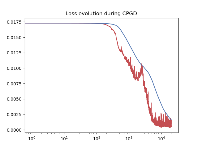
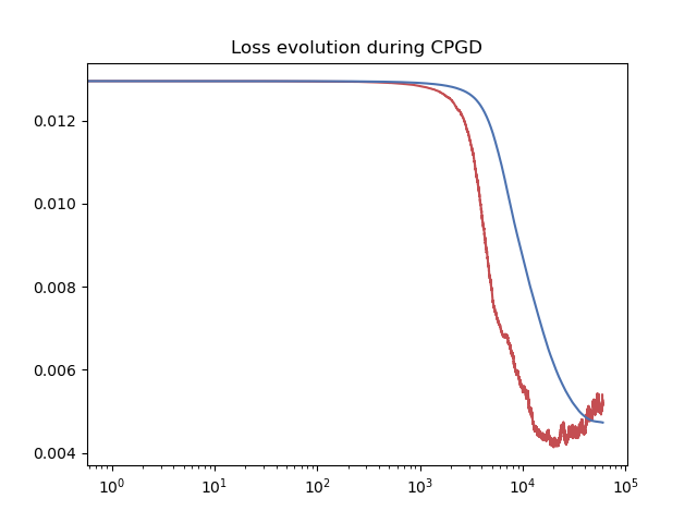
Figure 2: Evolution of the loss (log scale) with our S-CPGD algorithm (red) and its averaged counterpart (in blue) when using our methods on the mixture problems illustrated in Figure 1.

First, as indicated in Figure 2, we shall observe that the sequence $\hat{\bar{\nu}}_{K}$ always produces the desired smoothing effect all over the iterations of the algorithm, while slowing a bit the decrease of the loss function $J_{\nu}$ over the iterations. As a consequence, it seems more appropriate to use several long-range parallelized S-CPGD instead of a unique average thread of S-CPGD. In the same time, it may be remarked that our sequence $(\hat{\bar{\nu}}_{K})_{K\geq 1}$ is a rough approximation of the true Cesaro averaging that is studied in our paper and the numerical approximation introduced in (5.1) may not be as good as the true Cesaro sequence $(\bar{\nu}_{K})_{K\geq 1}$.

Second, as a classical phenomenon in machine learning when using stochastic approximation algorithm, or over-parameterized neural networks, our S-CPGD commonly generates some double-descent phenomena (see the 3 sub-figures of Figure 2) that translates some local minimizer escape of the swarm of particles.

Loss function: Averaging vs no averaging vs Deterministic

Figure 3 represents the evolution of the cost function with respect to the numerical cost which is a far better indicator than the number of iterations of the algorithm in our case since the S-CPGD algorithm is designed to be much more cheaper than the deterministic CPGD.

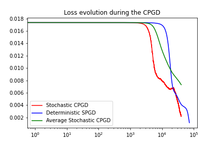
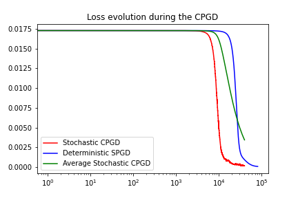
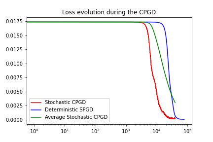
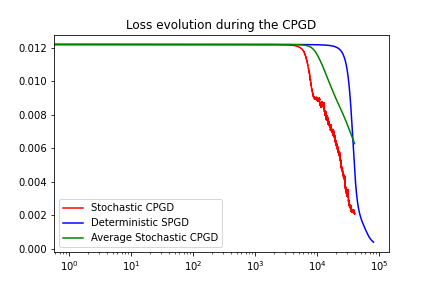
Figure 3: Evolution of the loss (log scale of the computational time) with our S-CPGD algorithm (red), its averaged counterpart (in green) and the deterministic CPGD (in blue) on the mixture problem of Figure 1 with 20 particles (top) and with 50 particles (bottom). As indicated in the text, and observed with the shift to the right of the blue curve when compared to the red one, the cost of our S-CPGD is much cheaper than the deterministic CPGD.

Figure 3 clearly illustrates the efficiency of our method with regards to the deterministic one as the red curve shows that the non-averaged S-CPGD produces comparable results as those obtained by CPGD with a significantly lower needs of computational cost: the red curve is clearly shifted on the left when compared to the blue one. It is furthermore possible to quantitatively assess the numerical gain produced by the S-CPGD when compared to the deterministic one: on our toy example, the deterministic CPGD requires approximately 4 more computations to attain the same decrease of the $J_{\nu}$, this effect being even amplified when the number of particles is increasing.

Loss function: Effect of the number of particles

In the meantime, we observe that the loss function benefits from a large number of particles (see the comparison between top and bottom lines of Figure 3) but this should be tempered by the increasing number of simulations, which varies linearly with the number of particles. We should finally observe that using a large number of particles seems to be important especially in difficult situations (as illustrated in the right column of Figure 3 where using 50 particles instead of 20 significantly improves the loss function, which is not the case on the right column of Figure 3.

The effect of the number of particles can also be illustrated while looking at the trajectories themselves of the particles as shown in Figure 4. We observe that the number of particles is a clear key parameter that strongly influences the success of the method. In our example of 5 components GMM, (last example in Figure 1), we see that a too small number of particles completely miss some components of the mixture while using a strongly over-parameterized set of particles permit to fully recover the support of the mixing distribution, even in the situation where some components of the mixture overlap.

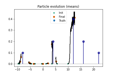
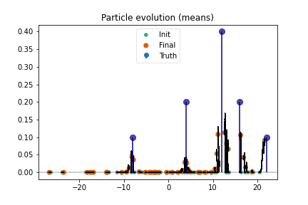
Figure 4: Trajectories of the particles of our S-CPGD algorithm in the third example of the mixture problem of Figure 1 with 5 modes. Left: trajectories using 10 particles. Right: Same with 50 particles. The l.h.s. shows the behaviour of S-CPGD when a too small number of particles is used. Particles concentrate around good positions but may miss some of the important locations of the mixture. The r.h.s. demonstrates that a sufficiently large number of particles is necessary to guarantee an exhaustive reconstruction of the mixing distribution.

From our brief numerical study, we can conclude that both sketching and batch subsampling with a stochastic gradient strategy appears to strongly improve the numerical cost of the Conic Particle Gradient Descent, which permits to increase the number of particles used in the mean field approximation. We also have shown that in some difficult inverse problem examples, a large number of particles seems necessary to perfectly recover the solution of the optimisation problem. It appears that the problem seriously benefits from a strong over-parametrisation, that may be handled with our cheap stochastic computing approach, which is not the case in a reasonnable time with the deterministic CPGD.

6 Proof of the main results

6.1 Proof of Proposition 4.1

Proof.

The principle of this proof is as follows. We identify two radii $R$ and $R_{0}$ such that $R<R_{0}$ for which the two following properties hold:

• If $\|\nu_{k}\|_{\mathrm{TV}}\leq R<R_{0}$, then $\|\nu_{k+1}\|_{\mathrm{TV}}\leq R_{0}$

• If $R\leq\|\nu_{k}\|_{\mathrm{TV}}\leq R_{0}$, then $\|\nu_{k+1}\|_{\mathrm{TV}}\leq\|\nu_{k}\|_{\mathrm{TV}}$.

We will establish these properties with a suitable choice for $R_{0}$ and a related condition on $\alpha$ as displayed in Proposition 4.1. The proof is divided into two steps.

Step 1: total variation norm recursion. Let $k\in\mathbb{N}$ be fixed, using an appropriate Taylor expansion, we get

$$\|\nu_{k+1}\|_{\mathrm{TV}} = \sum_{j=1}^{p}\omega_{j}^{k+1},$$

$$= \sum_{j=1}^{p}\omega_{j}^{k}e^{-\alpha\bm{J}_{\nu_{k}}^{\prime}(\bm{t}_{j}^{k},Z^{k+1})},$$

$$= \|\nu_{k}\|_{\mathrm{TV}}+\sum_{j=1}^{p}\omega_{j}^{k}\left(e^{-\alpha\bm{J}_{\nu_{k}}^{\prime}(\bm{t}_{j}^{k},Z^{k+1})}-1\right),$$

$$= \|\nu_{k}\|_{\mathrm{TV}}-\alpha\sum_{j=1}^{p}\omega_{j}^{k}\bm{J}_{\nu_{k}}^{\prime}(\bm{t}_{j}^{k},Z^{k+1})+\mathcal{R}(\alpha,\nu_{k},Z^{k+1}),$$

where $\mathcal{R}(\alpha,\nu_{k},Z^{k+1})$ is a remaining term whose value will be made precise later on. The last equality can be re-written as

$$\frac{\|\nu_{k+1}\|_{\mathrm{TV}}}{\|\nu_{k}\|_{\mathrm{TV}}}-1=\underbrace{-\alpha\sum_{j=1}^{p}\tilde{\omega}_{j}^{k}\bm{J}_{\nu_{k}}^{\prime}(\bm{t}_{j}^{k},Z^{k+1})}_{:=A_{1}}+\underbrace{\|\nu_{k}\|_{\mathrm{TV}}^{-1}\ \mathcal{R}(\alpha,\nu_{k},Z^{k+1})}_{:=A_{2}},$$ (6.1)

where for any $k\in\mathbb{N}$, $\tilde{\nu}_{k}:=\|\nu_{k}\|_{\mathrm{TV}}^{-1}\nu_{k}=\sum_{j=1}^{p}\tilde{\omega}_{j}^{k}\delta_{\bm{t}_{j}^{k}}$ and $\tilde{\omega}_{j}^{k}=\omega_{j}^{k}/\|\nu_{k}\|_{TV}$ for any $j\in\{1,\dots,p\}$. First, we concentrate our attention on the term $A_{1}$. Using (2.9),

$$A_{1} := -\alpha\sum_{j=1}^{p}\tilde{\omega}_{j}^{k}\bm{J}_{\nu_{k}}^{\prime}(\bm{t}_{j}^{k},Z^{k+1}),$$

$$= -\alpha\lambda-\alpha\|\nu_{k}\|_{TV}\int\bm{g}_{t,T^{k+1}}(U^{k+1})d\tilde{\nu}_{k}(t)+\alpha\int\bm{h}_{t}(V^{k+1})d\tilde{\nu}_{k}(t).$$

Using a rough bound, we get:

$$\int\bm{h}_{t}(V^{k+1})d\tilde{\nu}_{k}(t)\leq\|\bm{h}\|_{\infty}.$$ (6.2)

where we have used $\|\tilde{\nu}_{k}\|_{TV}=1$. Moreover,

$$\|\nu_{k}\|_{TV}\int\bm{g}_{t,T^{k+1}}(U^{k+1})d\tilde{\nu}_{k}(t) = \|\nu_{k}\|_{\mathrm{TV}}\sum_{j=1}^{p}\bm{\tilde{\omega}}_{j}^{k}\bm{g}_{\bm{t}_{j}^{k},T^{k+1}}(U^{k+1}),$$

$$\geq \|\nu_{k}\|_{\mathrm{TV}}\|\bm{g}\|_{Inf},$$

the last term being strictly positive thanks to our assumption. We eventually get, gathering the previous bounds

$$A_{1} \leq -\alpha\lambda-\alpha\|\bm{g}\|_{Inf}\|\nu_{k}\|_{\mathrm{TV}}+\alpha\|\bm{h}\|_{\infty}$$ (6.3)

$$= -\alpha\left[\lambda+\|\bm{g}\|_{Inf}\|\nu_{k}\|_{\mathrm{TV}}-\|\bm{h}\|_{\infty}\right].$$

Now, we turn our attention on the term $A_{2}$. Recall that

$$A_{2} := \|\nu_{k}\|_{\mathrm{TV}}^{-1}\ \mathcal{R}(\alpha,\nu_{k},Z^{k+1}),$$

$$= \sum_{j=1}^{p}\tilde{\omega}_{j}^{k}\left[e^{-\alpha\bm{J}_{\nu_{k}}^{\prime}(t_{j}^{k},Z^{k+1})}-1+\alpha\bm{J}_{\nu_{k}}^{\prime}(t_{j}^{k},Z^{k+1})\right].$$

Using the inequality

$$e^{-x}\leq 1-x+\frac{x^{2}}{2}e^{|x|}\quad\forall x\in\mathds{R},$$

we get

$$A_{2}\leq\sum_{j=1}^{p}\tilde{\omega}_{j}^{k}\left(\alpha\bm{J}_{\nu_{k}}^{\prime}(\bm{t}_{j}^{k},Z^{k+1})\right)^{2}\times e^{\alpha|\bm{J}_{\nu_{k}}^{\prime}(\bm{t}_{j}^{k},Z^{k+1})|}.$$

According to Lemma B.1, for any $l\in\{1,\dots,p\}$ and $k\in\mathbb{N}$,

$$\bm{J}_{\nu_{k}}^{\prime}(\bm{t}_{l}^{k},Z^{k+1})\leq\mathcal{C}_{1}(\|\nu_{k}\|_{\mathrm{TV}}+1)\quad\mathrm{with}\quad\mathcal{C}_{1}=\max(\|\bm{g}\|_{\infty};\|\bm{h}\|_{\infty}+\lambda).$$

Hence:

$$A_{2} \leq \sum_{j=1}^{p}\tilde{{\bm{\omega}}}_{j}^{k}\left(\alpha\mathcal{C}_{1}(\|\nu_{k}\|_{\mathrm{TV}}+1)\right)^{2}\times e^{\alpha(\mathcal{C}_{1}(\|\nu_{k}\|_{\mathrm{TV}}+1))},$$ (6.4)

$$\leq \left[\alpha\mathcal{C}_{1}(\|\nu_{k}\|_{\mathrm{TV}}+1)\right]^{2}e^{\alpha\mathcal{C}_{1}(\|\nu_{k}\|_{\mathrm{TV}}+1)}.$$

Assume that $\|\nu_{k}\|_{\mathrm{TV}}\leq R_{0}$ for some $R_{0}$. Gathering (6.1), (6.3) and (6.4), we obtain that:

$$\frac{\|\nu_{k+1}\|_{\mathrm{TV}}}{\|\nu_{k}\|_{\mathrm{TV}}}-1$$

$$\leq -\alpha\left[\lambda+\|\bm{g}\|_{Inf}\|\nu_{k}\|_{\mathrm{TV}}-\|\bm{h}\|_{\infty}\right]+\alpha^{2}\mathcal{C}_{1}^{2}(\|\nu_{k}\|_{\mathrm{TV}}+1)^{2}e^{\alpha\mathcal{C}_{1}(\|\nu_{k}\|_{\mathrm{TV}}+1)},$$

$$= -\alpha\left[\lambda+\|\bm{g}\|_{Inf}\|\nu_{k}\|_{\mathrm{TV}}-\left(\|\bm{h}\|_{\infty}+\alpha\mathcal{C}_{1}^{2}(\|\nu_{k}\|_{\mathrm{TV}}+1)^{2}e^{\alpha\mathcal{C}_{1}(\|\nu_{k}\|_{\mathrm{TV}}+1)}\right)\right],$$

$$\leq -\alpha\left[\lambda+\|\bm{g}\|_{Inf}\|\nu_{k}\|_{\mathrm{TV}}-\left(\|\bm{h}\|_{\infty}+\alpha\mathcal{C}_{1}^{2}(R_{0}+1)^{2}e^{\alpha\mathcal{C}_{1}(R_{0}+1)}\right)\right].$$

Step 2: calibration of $R,R_{0}$ and $\alpha$. We first make precise the value of the parameters involved in our bound and then verify that the stability property holds. We define $R_{0}$ and $R$ as:

$$R=\frac{\|\bm{h}\|_{\infty}+2\mathcal{C}_{1}}{\|\bm{g}\|_{Inf}},\quad R_{0}=R\left(1+\alpha(\|\bm{h}\|_{\infty}+2\mathcal{C}_{1})\right),\quad\mathrm{and}\quad\alpha\leq\frac{1}{2\mathcal{C}_{1}(R_{0}+1)^{2}},$$

where the constant $\mathcal{C}_{1}$ is introduced in (B.5). At this step, two different situations can occur.

• $1^{st}$ case: We consider the case where $\|\nu_{k}\|_{TV}\geq R$. In such a situation, the choice of $\alpha$ induces that:

  $$\frac{\|\nu_{k+1}\|_{\mathrm{TV}}}{\|\nu_{k}\|_{\mathrm{TV}}}-1 \leq -\alpha\left[\lambda+\|\bm{g}\|_{Inf}\|\nu_{k}\|_{\mathrm{TV}}-\left(\|\bm{h}\|_{\infty}+\alpha\mathcal{C}_{1}^{2}(R_{0}+1)^{2}e^{\alpha\mathcal{C}_{1}(R_{0}+1)}\right)\right],$$

  $$\leq -\alpha\left[\lambda+\|\bm{g}\|_{Inf}\|\nu_{k}\|_{\mathrm{TV}}-\left(\|\bm{h}\|_{\infty}+\mathcal{C}_{1}e^{\frac{1}{2(R_{0}+1)}}\right)\right],$$

  $$\leq -\alpha\left[\lambda+\|\bm{g}\|_{Inf}R-\left(\|\bm{h}\|_{\infty}+2\mathcal{C}_{1}\right)\right],$$

  $$\leq 0.$$

  The last inequality induces

  $$\|\nu_{k+1}\|_{\mathrm{TV}}\leq\|\nu_{k}\|_{\mathrm{TV}}\leq R_{0}.$$

• $2^{nd}$ case: We consider the situation where $\|\nu_{k}\|_{\mathrm{TV}}\leq R.$ With the same condition on $\alpha$, we use the rough bound

  $$\frac{\|\nu_{k+1}\|_{\mathrm{TV}}}{\|\nu_{k}\|_{\mathrm{TV}}}-1 \leq -\alpha\left[\lambda+\|\bm{g}\|_{Inf}\|\nu_{k}\|_{\mathrm{TV}}-\left(\|\bm{h}\|_{\infty}+\alpha\mathcal{C}_{1}^{2}(R_{0}+1)^{2}e^{\alpha\mathcal{C}_{1}(R_{0}+1)}\right)\right],$$

  $$\leq \alpha(\|\bm{h}\|_{\infty}+2\mathcal{C}_{1}).$$

  This implies that

  $$\|\nu_{k+1}\|_{TV} \leq \|\nu_{k}\|_{TV}(1+\alpha(\|\bm{h}\|_{\infty}+2\mathcal{C}_{1})),$$

  $$\leq R(1+\alpha(\|\bm{h}\|_{\infty}+2\mathcal{C}_{1}))=R_{0}.$$

Finally, we end the proof with an induction argument.∎

6.2 Proof of Theorem 4.1

6.2.1 The shadow sequence

Consider an integer $k\geq 0$ and the map $\mathcal{T}_{k+1}$ defined as:

$$\forall t\in\mathcal{X}\qquad\mathcal{T}_{k+1}(t)=t-\eta\bm{D}_{\nu_{k}}(t,Z^{k+1}),$$ (6.5)

where $(Z^{k+1})_{k\geq 0}$ is the sequence of random variables sampled in Algorithm 1 and used in Equations (2.14) and (2.15). The sequence of maps $(\mathcal{T}_{k+1})_{k\geq 0}$ only acts on the positions of $\mathcal{X}$ and is built with the random sequence $(\nu_{k})_{k\geq 1}$.

Using $(\mathcal{T}_{k+1})_{k\geq 0}$, we then define the shadow sequence $(\nu^{\varepsilon}_{k})_{k\geq 1}$ obtained through an iterative push-forward from a given initialisation measure $\nu_{0}^{\epsilon}\in\mathcal{M}(\mathcal{X})_{+}$ with the sequence of maps $(\mathcal{T}_{k})_{k\geq 1}$. More formally, we set in a iterative way

$$\nu^{\varepsilon}_{k+1}=\mathcal{T}_{k+1}^{\#}(\nu^{\varepsilon}_{k})\qquad\forall k\in\mathbb{N}^{\star},$$ (6.6)

where, for any continuous function $\psi$,

$$\int_{\mathcal{X}}\psi d\mathcal{T}_{k+1}^{\#}(\nu)=\int_{\mathbb{}}\psi(\mathcal{T}_{k+1}(.))d\nu\quad\forall\nu\in\mathcal{M}(\mathcal{X}).$$

The measure $\nu_{0}^{\varepsilon}$ will be defined carefully at the very end of our study. Roughly speaking, the shadow sequence $(\nu^{\varepsilon}_{k})_{k\geq 1}$ moves exactly like $(\nu_{k})_{k\geq 1}$ and will share the same support, but the weights on the particles for the sequence $(\nu^{\varepsilon}_{k})_{k\geq 1}$ will be optimised to allow for a good approximation of $\mu^{\star}$. In particular, if we decompose the initial measure $\nu_{0}$ as

$$\nu_{0}=\sum_{j=1}^{p}\omega_{j}\delta_{{\bm{t}}^{0}_{j}},$$

then we can write $\nu_{0}^{\varepsilon}=\nu(\mathds{W}^{\varepsilon},{\bm{t}}^{0})$, so that:

$$\nu_{0}^{\varepsilon}=\sum_{j=1}^{p}\omega_{j}^{\varepsilon}\delta_{{\bm{t}}^{0}_{j}},$$

for some weights $(\omega_{j}^{\epsilon})_{j=1..p}$ that will be chosen in an appropriate way.

6.2.2 Excess risk decomposition

The starting point is Proposition B.1 that is used with $\nu=\nu_{k}$ and $\sigma=\mu^{\star}-\nu_{k}$. We write:

$$J(\nu_{k})-J(\mu^{\star}) =\int_{\mathcal{X}}J^{\prime}_{\nu_{k}}\text{d}[\nu_{k}-\mu^{\star}]-\frac{1}{2}\|\Phi(\mu^{\star}-\nu_{k})\|^{2}_{\mathds{H}}$$

$$=\underbrace{\int_{\mathcal{X}}J^{\prime}_{\nu_{k}}\text{d}[\nu_{k}-\nu^{\varepsilon}_{k}]}_{:=\text{①}}+\underbrace{\int_{\mathcal{X}}J^{\prime}_{\nu_{k}}\text{d}[\nu^{\varepsilon}_{k}-\mu^{\star}]}_{:=\text{②}}-\frac{1}{2}\|\Phi(\mu^{\star}-\nu_{k})\|^{2}_{\mathds{H}}$$ (6.7)

where $(\nu^{\varepsilon}_{k})_{k\geq 1}$ is the auxiliary shadow sequence of measures introduced in (6.6). First, we establish that the mirror descent adapts the weights of $(\nu_{k})_{k\geq 1}$ to those of the shadow sequence $(\nu^{\varepsilon}_{k})_{k\geq 1}$. For any $\mu_{1},\mu_{2}\in\mathcal{M}(\mathcal{X})_{+}$, we introduce the following entropy:

$$\mathcal{H}(\mu_{1},\mu_{2})=-\int_{\mathcal{X}}\log\left(\frac{\text{d}\mu_{1}}{\text{d}\mu_{2}}\right)\text{d}\mu_{2}-\|\mu_{2}\|_{\mathrm{TV}}+\|\mu_{1}\|_{\mathrm{TV}}.$$ (6.8)

The next proposition focuses on the first term of Equation (6.7).

Proposition 6.1.

Term ① of Equation (6.7) may be decomposed as:

$$\text{①}=\int_{\mathcal{X}}J^{\prime}_{\nu_{k}}\text{d}[\nu_{k}-\nu^{\varepsilon}_{k}] =\frac{1}{\alpha}\left[\mathcal{H}(\nu_{k},\nu^{\varepsilon}_{k})-\mathcal{H}(\nu_{k+1},\nu^{\varepsilon}_{k+1})\right]$$

$$+\frac{1}{\alpha}\sum_{j=1}^{p}\omega_{j}^{k}\left[\alpha J^{\prime}_{\nu_{k}}({\bm{t}}_{j}^{k})+e^{-\alpha J^{\prime}_{\nu_{k}}({\bm{t}}_{j}^{k},Z^{k+1})}-1\right]+\sum_{j=1}^{p}\omega_{j}^{\varepsilon}\xi_{\nu_{k}}({\bm{t}}_{j}^{k},Z^{k+1})$$

Proof.

Since both measures $\nu_{k}$ and $\nu^{\varepsilon}_{k}$ share the same particle locations $\bm{t}^{k}$, we can remark that

$$\text{①}=\int_{\mathcal{X}}J^{\prime}_{\nu_{k}}\text{d}[\nu_{k}-\nu^{\varepsilon}_{k}]=\sum_{j=1}^{p}[\omega_{j}^{k}-\omega_{j}^{\varepsilon}]J^{\prime}_{\nu_{k}}({\bm{t}}_{j}^{k})$$ (6.9)

We then observe from Equation (2.14) that:

$$\omega_{j}^{k+1}=\omega_{j}^{k}e^{-\alpha\bm{J}^{\prime}_{\nu_{k}}({\bm{t}}_{j}^{k},Z^{k+1})}\quad\Rightarrow\quad J^{\prime}_{\nu_{k}}({\bm{t}}_{j}^{k},Z^{k+1})=-\frac{1}{\alpha}\log\left(\frac{\omega_{j}^{k+1}}{\omega_{j}^{k}}\right).$$

Using now Equation (2.10), we observe that:

$$J^{\prime}_{\nu_{k}}({\bm{t}}_{j}^{k})=-\frac{1}{\alpha}\log\left(\frac{\omega_{j}^{k+1}}{\omega_{j}^{k}}\right)-\xi_{\nu_{k}}({\bm{t}}_{j}^{k},Z^{k+1}).$$

We then use the previous equality in (6.9) and obtain that:

① $$=\sum_{j=1}^{p}\left(\omega_{j}^{k}J^{\prime}_{\nu_{k}}({\bm{t}}_{j}^{k})-\omega_{j}^{\varepsilon}\left[-\frac{1}{\alpha}\log\left(\frac{\omega_{j}^{k+1}}{\omega_{j}^{k}}\right)-\xi_{\nu_{k}}({\bm{t}}_{j}^{k},Z^{k+1})\right]\right),$$

$$=\sum_{j=1}^{p}\left(\omega_{j}^{k}J^{\prime}_{\nu_{k}}({\bm{t}}_{j}^{k})+\omega_{j}^{\varepsilon}\frac{1}{\alpha}\log\left(\frac{\omega_{j}^{k+1}}{\omega_{j}^{k}}\right)\right)+\sum_{j=1}^{p}\omega_{j}^{\varepsilon}\xi_{\nu_{k}}({\bm{t}}_{j}^{k},Z^{k+1})$$

$$=\frac{1}{\alpha}\sum_{j=1}^{p}\left(\alpha\omega_{j}^{k}J^{\prime}_{\nu_{k}}({\bm{t}}_{j}^{k})+\omega_{j}^{\varepsilon}\left[\log\left(\frac{\omega_{j}^{k+1}}{\omega_{j}^{\varepsilon}}\right)-\log\left(\frac{\omega_{j}^{k}}{\omega_{j}^{\varepsilon}}\right)\right]\right)+\sum_{j=1}^{p}\omega_{j}^{\varepsilon}\xi_{\nu_{k}}({\bm{t}}_{j}^{k},Z^{k+1}).$$

We use the entropy $\mathcal{H}$ introduced in Equation (6.8) and deduce that:

① $$=\frac{1}{\alpha}\sum_{j=1}^{p}\left[\alpha\omega_{j}^{k}J^{\prime}_{\nu_{k}}({\bm{t}}_{j}^{k})+\omega_{j}^{k+1}-\omega_{j}^{k}\right]+\frac{\mathcal{H}(\nu_{k},\nu^{\varepsilon}_{k})-\mathcal{H}(\nu_{k+1},\nu^{\varepsilon}_{k+1})}{\alpha}+\sum_{j=1}^{p}\omega_{j}^{\varepsilon}\xi_{\nu_{k}}({\bm{t}}_{j}^{k},Z^{k+1})$$

$$=\frac{1}{\alpha}\sum_{j=1}^{p}\omega_{j}^{k}\left[\alpha J^{\prime}_{\nu_{k}}({\bm{t}}_{j}^{k})+e^{-\alpha\bm{J}^{\prime}_{\nu_{k}}({\bm{t}}_{j}^{k},Z^{k+1})}-1\right]+\frac{\mathcal{H}(\nu_{k},\nu^{\varepsilon}_{k})-\mathcal{H}(\nu_{k+1},\nu^{\varepsilon}_{k+1})}{\alpha}+\sum_{j=1}^{p}\omega_{j}^{\varepsilon}\xi_{\nu_{k}}({\bm{t}}_{j}^{k},Z^{k+1}).$$

We then obtain the conclusion of the proof. ∎

Now, we study the second term of Equation (6.7), which is an “approximation” term. We essentially follow the same methodology proposed in Chizat (2022) but we use the specificity of our model to properly analyze this term. For this purpose, we use the BL norm (over functions) and dual norm (over measures) introduced in Chizat (2022), defined as:

$$\forall f:\mathcal{X}\rightarrow\mathds{R}\qquad\|f\|_{BL}=\|f\|_{\infty}+\|f\|_{Lip},$$ (6.10)

where $\|.\|_{\infty}$ refers to the supremum norm over $\mathcal{X}$, $\|.\|_{Lip}$ to the Lipschitz constant for $f$, and

$$\forall\nu\in\mathcal{M}(\mathcal{X})_{+}\qquad\|\nu\|^{*}_{BL}=\sup_{\|f\|_{BL}\leq 1}\int f\text{d}\nu.$$ (6.11)

We also introduce the constant $Lip(\varphi)$ defined as

$$Lip(\varphi)=\sup_{s,t\in\mathcal{X}}\frac{\|\varphi_{t}-\varphi_{s}\|_{\mathds{H}}}{\|t-s\|_{\mathcal{X}}}.$$

Using these notation, we can propose a bound on the second term of Equation (6.7) as displayed in the following proposition.

Proposition 6.2.

The approximation term ② satisfies:

$$\forall k\geq 1\qquad\text{②}=\int_{\mathcal{X}}J^{\prime}_{\nu_{k}}\text{d}[\nu^{\varepsilon}_{k}-\mu^{\star}]\leq\mathfrak{A}_{k}\|\nu^{\varepsilon}_{k}-\mu^{\star}\|_{BL}^{*}\quad\text{a.s.}$$

where $\mathfrak{A}_{k}$ is given by:

$$\mathfrak{A}_{k}=\mathcal{C}_{0}(\|\nu_{k}\|_{TV}+1)+Lip(\varphi)\left[\|\nu_{k}\|_{TV}\|\varphi\|_{\infty,\mathds{H}}+\|y\|_{\mathds{H}}\right],$$ (6.12)

where

$$\mathcal{C}_{0}=\max(\lambda+\|\varphi\|_{\infty,\mathds{H}}\|y\|_{\mathds{H}};\|\varphi\|_{\infty,\mathds{H}}^{2}).$$

Proof.

We can immediately remark that

$$\text{②}=\int_{\mathcal{X}}J^{\prime}_{\nu_{k}}\text{d}[\nu^{\varepsilon}_{k}-\mu^{\star}]\leq\|J_{\nu_{k}}^{\prime}\|_{BL}\|\nu^{\varepsilon}_{k}-\mu^{\star}\|_{BL}^{*}.$$

Then, according to Lemma B.1,

$$\|J_{\nu_{k}}^{\prime}\|_{BL}=\|J_{\nu_{k}}^{\prime}\|_{\infty}+\|J_{\nu_{k}}^{\prime}\|_{Lip}\leq\mathcal{C}_{0}(\|\nu_{k}\|_{TV}+1)+\|J_{\nu_{k}}^{\prime}\|_{Lip}.$$

To conclude the proof, we have to propose an upper bound on $\|J_{\nu_{k}}^{\prime}\|_{Lip}$. For any $s,t\in\mathcal{X}$ we have

$$|J_{\nu_{k}}^{\prime}(s)-J_{\nu_{k}}^{\prime}(t)| = \left|\sum_{j=1}^{p}\omega_{j}^{k}\langle\varphi_{t}-\varphi_{s},\varphi_{\bm{t}_{j}^{k}}\rangle_{\mathds{H}}-\langle\varphi_{t}-\varphi_{s},\bm{y}\rangle_{\mathds{H}}\right|,$$

$$\leq \sum_{j=1}^{p}\omega_{j}^{k}\|\varphi_{t}-\varphi_{s}\|_{\mathds{H}}\|\varphi_{\bm{t}_{j}^{k}}\|_{\mathds{H}}+\|\varphi_{t}-\varphi_{s}\|_{\mathds{H}}\|\bm{y}\|_{\mathds{H}},$$

$$\leq Lip(\varphi)\left[\|\nu_{k}\|_{TV}\|\varphi\|_{\infty,\mathds{H}}+\|y\|_{\mathds{H}}\right]\times\|t-s\|_{\mathcal{X}}.$$

The results is obtained by gathering the previous bounds. ∎

We finally introduce a key term that quantifies the way where $\mu^{\star}$ can be approximated by a discrete measure. This term, denoted by $\mathcal{Q}$, is defined as

$$\mathcal{Q}_{\mu^{\star},\nu_{0}}(\tau):=\inf_{\mu\in\mathcal{M}(\mathcal{X})_{+}}\left[\|\mu^{\star}-\mu\|_{BL}^{*}+\frac{1}{\tau}\mathcal{H}(\mu,\nu_{0})\right]\quad\forall\tau>0.$$ (6.13)

6.2.3 Proof of Theorem 4.1

Proof.

Below, $\mathfrak{C}$ will refer to a constant independent on $K$ and $p$, whose value may change from line to line. The proof is decomposed into three steps.

Step 1: Decomposition of the excess risk with the convexity of $J$.

We denote by $(\mathfrak{F}_{k})_{k\geq 0}$ the natural canonical filtration associated to the sequence of random variables $(Z^{k})_{k\geq 0}$. The next upper bound is a consequence of the relationship (6.7) and Propositions 6.1, 6.2. We have

$$J(\nu_{k})-J(\mu^{\star}) \leq\frac{\mathcal{H}(\nu_{k},\nu^{\varepsilon}_{k})-\mathcal{H}(\nu_{k+1},\nu^{\varepsilon}_{k+1})}{\alpha}+\mathfrak{A}_{k}\|\nu^{\varepsilon}_{k}-\mu^{\star}\|_{BL}^{*}$$

$$+\frac{1}{\alpha}\sum_{j=1}^{p}\omega_{j}^{k}\left[\alpha J^{\prime}_{\nu_{k}}({\bm{t}}_{j}^{k})+e^{-\alpha J^{\prime}_{\nu_{k}}({\bm{t}}_{j}^{k},Z^{k+1})}-1\right]+\sum_{j=1}^{p}\omega_{j}^{\varepsilon}\xi_{\nu_{k}}({\bm{t}}_{j}^{k},Z^{k+1}).$$

We then use a telescopic sum argument and obtain that:

$$\sum_{k=0}^{K}\left(J(\nu_{k})-J(\mu^{\star})\right) \leq\frac{\mathcal{H}(\nu_{0},\nu_{0}^{\varepsilon})}{\alpha}+\sum_{k=0}^{K}\mathfrak{A}_{k}\|\nu^{\varepsilon}_{k}-\mu^{\star}\|_{BL}^{*}$$

$$+\frac{1}{\alpha}\sum_{k=0}^{K}\sum_{j=1}^{p}\omega_{j}^{k}\left[\alpha J^{\prime}_{\nu_{k}}({\bm{t}}_{j}^{k})+e^{-\alpha J^{\prime}_{\nu_{k}}({\bm{t}}_{j}^{k},Z^{k+1})}-1\right]+\sum_{k=0}^{K}\sum_{j=1}^{p}\omega_{j}^{\varepsilon}\xi_{\nu_{k}}({\bm{t}}_{j}^{k},Z^{k+1}).$$

Finally, using the convexity of $J$, the Cesaro average defined by:

$$\bar{\nu}_{K}=\frac{1}{K+1}\sum_{k=0}^{K}\nu_{k},$$ (6.14)

satisfies:

$$J(\bar{\nu}_{K})-J(\mu^{\star}) \leq\frac{\mathcal{H}(\nu_{0},\nu_{0}^{\varepsilon})}{\alpha(K+1)}+\frac{\sum_{k=0}^{K}\mathfrak{A}_{k}\|\nu^{\varepsilon}_{k}-\mu^{\star}\|_{BL}^{*}}{K+1}$$

$$+\frac{\sum_{k=0}^{K}\sum_{j=1}^{p}\omega_{j}^{k}\left[\alpha J^{\prime}_{\nu_{k}}({\bm{t}}_{j}^{k})+e^{-\alpha J^{\prime}_{\nu_{k}}({\bm{t}}_{j}^{k},Z^{k+1})}-1\right]}{\alpha(K+1)}+\frac{\sum_{k=0}^{K}\sum_{j=1}^{p}\omega_{j}^{\varepsilon}\xi_{\nu_{k}}({\bm{t}}_{j}^{k},Z^{k+1})}{K+1}$$

$$\leq\frac{\mathcal{H}(\nu_{0},\nu_{0}^{\varepsilon})}{\alpha K}+\frac{\sum_{k=0}^{K}\mathfrak{A}_{k}\left[\|\nu_{0}^{\varepsilon}-\mu^{\star}\|^{*}_{BL}+\sum_{\ell=0}^{k-1}\|\nu_{\ell+1}^{\varepsilon}-\nu_{\ell}^{\varepsilon}\|_{BL}^{*}\right]}{K}$$

$$+\frac{\sum_{k=0}^{K}\sum_{j=1}^{p}\omega_{j}^{k}\left[\alpha J^{\prime}_{\nu_{k}}({\bm{t}}_{j}^{k})+e^{-\alpha J^{\prime}_{\nu_{k}}({\bm{t}}_{j}^{k},Z^{k+1})}-1\right]}{\alpha K}+\frac{\sum_{k=0}^{K}\sum_{j=1}^{p}\omega_{j}^{\varepsilon}\xi_{\nu_{k}}({\bm{t}}_{j}^{k},Z^{k+1})}{K}$$

where we used the triangle inequality on the telescopic decomposition

$$\nu^{\varepsilon}_{k}-\mu^{\star}=(\nu^{\varepsilon}_{k}-\nu_{k-1}^{\varepsilon})+(\nu_{k-1}^{\varepsilon}-\nu_{k-2}^{\varepsilon})+\ldots+(\nu_{0}^{\varepsilon}-\mu^{\star}).$$

We then take the expectation and use in particular a standard conditional expectation argument. Since $\mathbb{E}[\xi_{\nu_{k}}({\bm{t}}_{j}^{k},Z^{k+1})|\mathfrak{F}_{k}]=0$, we deduce that:

$$\mathbb{E}\left[J(\bar{\nu}_{K})-J(\mu^{\star})\right] \leq\frac{\mathcal{H}(\nu_{0},\nu_{0}^{\varepsilon})}{\alpha(K+1)}+\overbrace{\|\nu_{0}^{\varepsilon}-\mu^{\star}\|^{*}_{BL}\frac{\sum_{k=0}^{K}\mathbb{E}[\mathfrak{A}_{k}]}{K+1}}^{:=A_{1}}+\overbrace{\frac{\sum_{k=0}^{K}\mathbb{E}\left[\mathfrak{A}_{k}\sum_{\ell=0}^{k-1}\|\nu_{\ell+1}^{\varepsilon}-\nu_{\ell}^{\varepsilon}\|_{BL}^{*}\right]}{K+1}}^{:=A_{2}}$$

$$+\underbrace{\frac{\sum_{k=0}^{K}\sum_{j=1}^{p}\mathbb{E}\left[\omega_{j}^{k}\left[\alpha J^{\prime}_{\nu_{k}}({\bm{t}}_{j}^{k})+e^{-\alpha J^{\prime}_{\nu_{k}}({\bm{t}}_{j}^{k},Z^{k+1})}-1\right]\right]}{\alpha(K+1)}}_{:=A_{3}}.$$ (6.15)

Step 2a: Study of $A_{1}$. We use the definition of $\mathfrak{A}_{k}$ in Equation (6.12) and observe that $\mathfrak{A}_{k}\leq\mathfrak{C}(1+\|\nu_{k}\|_{\mathrm{TV}})$. We then use Proposition 4.1 and conclude that:

$$\mathbb{E}[A_{1}]=\|\nu_{0}^{\varepsilon}-\mu^{\star}\|^{*}_{BL}\frac{\sum_{k=0}^{K}\mathbb{E}[\mathfrak{A}_{k}]}{K+1}\leq\mathfrak{C}R_{0}\|\nu_{0}^{\varepsilon}-\mu^{\star}\|^{*}_{BL}.$$ (6.16)

Step 2b: Study of $A_{2}$. We focus on the shadow sequence that involves $\nu_{\ell+1}^{\varepsilon}-\nu_{\ell}^{\varepsilon}$ and observe that:

$$\|\nu_{\ell+1}^{\varepsilon}-\nu_{\ell}^{\varepsilon}\|_{BL}^{*} =\sup_{\|\psi\|_{BL}\leq 1}\int_{\mathcal{X}}\psi(t)\text{d}[\nu^{\varepsilon}_{\ell+1}-\nu^{\varepsilon}_{\ell}](t)$$

$$=\sup_{\|\psi\|_{BL}\leq 1}\sum_{j=1}^{p}\omega_{j}^{\varepsilon}[\psi({\bm{t}}_{j}^{\ell+1})-\psi({\bm{t}}_{j}^{\ell})]$$

$$\leq\sum_{j=1}^{p}\omega_{j}^{\varepsilon}\|{\bm{t}}_{j}^{\ell+1}-{\bm{t}}_{j}^{\ell}\|_{\mathcal{X}}$$

$$=\eta\sum_{j=1}^{p}\omega_{j}^{\varepsilon}\|{\bm{D}}_{\nu_{\ell}}(\mathds{T}^{\ell},Z^{\ell+1})_{j}\|_{\mathcal{X}}$$

$$\leq C\eta\sum_{j=1}^{p}\omega_{j}^{\varepsilon}(1+\|\nu_{\ell}\|_{\mathrm{TV}})$$

$$=C\eta\|\nu_{0}^{\varepsilon}\|_{\mathrm{TV}}(1+\|\nu_{\ell}\|_{\mathrm{TV}}),$$ (6.17)

where we used the almost sure upper bound in Proposition C.1. A simple sum yields:

$$\frac{\sum_{k=0}^{K}\mathfrak{A}_{k}\sum_{\ell=0}^{k-1}\|\nu_{\ell+1}^{\varepsilon}-\nu_{\ell}^{\varepsilon}\|_{BL}^{*}}{K+1} \leq\mathfrak{C}\eta\|\nu_{0}^{\varepsilon}\|_{\mathrm{TV}}\frac{\sum_{k=0}^{K}\mathfrak{A}_{k}\sum_{\ell=1}^{k}\left(1+\|\nu_{\ell}\|_{\mathrm{TV}}\right)}{K+1}$$

$$\leq\mathfrak{C}\eta\|\nu_{0}^{\varepsilon}\|_{\mathrm{TV}}\frac{\sum_{k=0}^{K}(1+\|\nu_{k}\|_{\mathrm{TV}})\sum_{\ell=1}^{k}\left(1+\|\nu_{\ell}\|_{\mathrm{TV}}\right)}{K+1},$$

for $\mathfrak{C}$ large enough. Again, we apply Proposition 4.1 and compute the expectation of the previous term. We then observe that:

$$\mathbb{E}[A_{2}]=\frac{\sum_{k=0}^{K}\mathbb{E}\left[\mathfrak{A}_{k}\sum_{\ell=0}^{k-1}\|\nu_{\ell+1}^{\varepsilon}-\nu_{\ell}^{\varepsilon}\|_{BL}^{*}\right]}{K+1}\leq\mathfrak{C}R_{0}^{2}\eta\|\nu_{0}^{\varepsilon}\|_{\mathrm{TV}}K.$$ (6.18)

Step 2c: Study of $A_{3}$. This last term deserves a specific study. We use a conditional expectation argument and observe that, for any $k\in\{0,\dots,K\}$, $j\in\{1,\dots,p\}$,

$$\mathbb{E}\left[\omega_{j}^{k}\left.\left[\alpha J^{\prime}_{\nu_{k}}({\bm{t}}_{j}^{k})+e^{-\alpha J^{\prime}_{\nu_{k}}({\bm{t}}_{j}^{k},Z^{k+1})}-1\right]\right|\mathfrak{F}_{k}\right]=\omega_{j}^{k}\mathbb{E}\left[\left.\left[\alpha J^{\prime}_{\nu_{k}}({\bm{t}}_{j}^{k})+e^{-\alpha J^{\prime}_{\nu_{k}}({\bm{t}}_{j}^{k},Z^{k+1})}-1\right]\right|\mathfrak{F}_{k}\right].$$

We then apply Proposition C.2 ang get:

$$\mathbb{E}\left[\omega_{j}^{k}\left.\left[\alpha J^{\prime}_{\nu_{k}}({\bm{t}}_{j}^{k})+e^{-\alpha J^{\prime}_{\nu_{k}}({\bm{t}}_{j}^{k},Z^{k+1})}-1\right]\right|\mathfrak{F}_{k}\right]\leq\mathfrak{C}\omega_{j}^{k}\alpha^{2}(1+\|\nu_{k}\|_{\mathrm{TV}}^{2})$$

We then sum the previous upper bounds from $0$ to $K$ with a global expectation and Proposition 4.1. We obtain that:

$$\mathbb{E}[A_{3}]=\frac{\sum_{k=0}^{K}\sum_{j=1}^{p}\mathbb{E}\left[\omega_{j}^{k}\left[\alpha J^{\prime}_{\nu_{k}}({\bm{t}}_{j}^{k})+e^{-\alpha J^{\prime}_{\nu_{k}}({\bm{t}}_{j}^{k},Z^{k+1})}-1\right]\right]}{\alpha(K+1)}\leq\mathfrak{C}\alpha R_{0}^{3}.$$ (6.19)

Step 3: End of the proof.

We gather Equations (6.16), (6.18), (6.19) and obtain that:

$$\mathbb{E}\left[J(\bar{\nu}_{K})-J(\mu^{\star})\right]\leq\frac{\mathcal{H}(\nu_{0},\nu_{0}^{\varepsilon})}{\alpha K}+\mathfrak{C}R_{0}\|\nu_{0}^{\varepsilon}-\mu^{\star}\|_{BL}^{*}+\mathfrak{C}R_{0}^{2}\left[\eta\|\nu_{0}^{\varepsilon}\|_{\mathrm{TV}}K+\alpha R_{0}\right].$$

We then use the definition of $\mathcal{Q}$ given in Equation (6.13) and observe that if $\nu_{0}^{\varepsilon}$ is chosen in an optimal way, as given in Proposition C.3, then:

$$\mathbb{E}\left[J(\bar{\nu}_{K})-J(\mu^{\star})\right] \leq R_{0}\mathcal{Q}_{\mu^{\star},\nu_{0}}(\alpha KR_{0})+\mathfrak{C}R_{0}^{2}\left[\eta\|\mu^{\star}\|_{\mathrm{TV}}K+\alpha R_{0}\right]$$

$$\leq\mathfrak{C}\|\mu^{\star}\|_{\mathrm{TV}}\left[\frac{d\left(1+\log\frac{\alpha KR_{0}}{2d}+\frac{\log|\mathcal{X}|}{d}\right)}{\alpha K}+\frac{\alpha R_{0}^{3}}{\|\mu^{\star}\|_{\mathrm{TV}}}+R_{0}^{2}\eta K\right],$$

where we have used the relationship $\|\nu_{0}^{\varepsilon}\|_{TV}=\|\mu^{\star}\|_{TV}$. The choices

$$\alpha=\sqrt{\frac{d\|\mu^{\star}\|_{\mathrm{TV}}}{R_{0}^{3}K}}\quad\mathrm{and}\quad\eta=\sqrt{\frac{dR_{0}}{K^{3}\|\mu^{\star}\|_{\mathrm{TV}}}}$$

then leads to

$$\mathbb{E}\left[J(\bar{\nu}_{K})-J(\mu^{\star})\right]\leq\mathfrak{C}\sqrt{\frac{d\|\mu^{\star}\|_{\mathrm{TV}}R_{0}^{3}}{K}}\left[\log(d\|\mu^{\star}\|_{\mathrm{TV}}R_{0}^{3}K)+\frac{\log(|\mathcal{X}|)}{d}\right].$$

∎

6.3 Proof of Theorem 4.2

Proof.

The proof is splitted into three parts, and relies on a contraction argument with conditional expectation. In what follows, we will choose $\alpha$ such that $\alpha\mathcal{C}_{1}(R_{0}+1)<1$ where $\mathcal{C}_{1}$ is involved in Lemma B.1, and we shall use $|e^{h}-1|\leq 2|h|$ which is valid when $|h|\leq 1$. We will frequently apply this inequality with $h=-\alpha J_{\nu_{k}}^{\prime}({\bm{t}}_{j}^{k},Z^{k+1})$.

Step 1: One-step evolution and second order term. Let $k\in\mathbb{N}^{\star}$ be fixed. According to Proposition B.1:

$$J(\nu_{k+1})-J(\nu_{k})=\int_{\mathcal{X}}J_{\nu_{k}}^{\prime}d(\nu_{k+1}-\nu_{k})+\frac{1}{2}\|\Phi(\nu_{k+1}-\nu_{k})\|_{\mathds{H}}^{2}.$$

Introducing the measure $\tilde{\nu}_{k+1}=\sum_{j=1}^{p}\omega_{j}^{k+1}\delta_{\bm{t}_{j,k}}$, we deduce that:

$$\|\Phi(\nu_{k+1}-\nu_{k})\|_{\mathds{H}}^{2} = \|\Phi(\nu_{k+1}-\tilde{\nu}_{k+1}+\tilde{\nu}_{k+1}-\nu_{k})\|_{\mathds{H}}^{2},$$

$$\leq 2\|\Phi(\nu_{k+1}-\tilde{\nu}_{k+1})\|_{\mathds{H}}^{2}+2\|\Phi(\tilde{\nu}_{k+1}-\nu_{k})\|_{\mathds{H}}^{2}$$

First remark that,

$$\|\Phi(\nu_{k+1}-\tilde{\nu}_{k+1})\|_{\mathds{H}}^{2} = \left\|\sum_{j=1}^{p}\omega_{j}^{k+1}(\varphi_{\bm{t}_{j}^{k+1}}-\varphi_{\bm{t}_{j}^{k}})\right\|_{\mathds{H}}^{2},$$

$$\leq \sum_{j=1}^{p}\omega_{j}^{k+1}\times\sum_{j=1}^{p}\omega_{j}^{k+1}\|\varphi_{\bm{t}_{j}^{k+1}}-\varphi_{\bm{t}_{j}^{k}}\|_{\mathds{H}}^{2},$$

$$\leq Lip(\varphi)\|\nu_{k+1}\|_{\mathrm{TV}}\sum_{j=1}^{p}\omega_{j}^{k+1}\|\bm{t}_{j}^{k+1}-\bm{t}_{j}^{k}\|^{2}_{\mathcal{X}}.$$

We then use the update of $\mathds{T}^{k}$ to $\mathds{T}^{k+1}$ that is given in (2.15) and obtain that:

$$\|\Phi(\nu_{k+1}-\tilde{\nu}_{k+1})\|_{\mathds{H}}^{2}\leq Lip(\varphi)\|\nu_{k+1}\|_{\mathrm{TV}}\eta^{2}\sum_{j=1}^{p}\omega_{j}^{k}\|D_{\nu_{k}}({\bm{t}}_{j}^{k},Z^{k+1})\|^{2}_{\mathcal{X}}.$$ (6.20)

In the same time, using (2.14), we obtain that:

$$\|\Phi(\tilde{\nu}_{k+1}-\nu_{k})\|_{\mathds{H}}^{2} = \left\|\sum_{j=1}^{p}(\omega_{j}^{k+1}-\omega_{j}^{k})\varphi_{\bm{t}_{j,k}}\right\|_{\mathds{H}}^{2},$$

$$= \left\|\sum_{j=1}^{p}\omega_{j}^{k}(e^{-\alpha J_{\nu_{k}}^{\prime}({\bm{t}}_{j}^{k},Z^{k+1})}-1)\varphi_{\bm{t}_{j,k}}\right\|_{\mathds{H}}^{2},$$

$$\leq \sum_{j=1}^{p}\omega_{j}^{k}\times\sum_{j=1}^{p}\omega_{j}^{k}(e^{-\alpha J_{\nu_{k}}^{\prime}({\bm{t}}_{j}^{k},Z^{k+1})}-1)^{2}\left\|\varphi_{\bm{t}_{j,k}}\right\|_{\mathds{H}}^{2},$$

where the last line comes from the Jensen inequality. We then observe from Lemma B.1 that $J_{\nu_{k}}^{\prime}({\bm{t}}_{j}^{k},Z^{k+1})$ is a bounded term so that if $\alpha$ is chosen such that $\alpha\mathcal{C}_{1}(R_{0}+1)<1$, then a constant $C_{\varphi}$ large enough exists such that:

$$\|\Phi(\tilde{\nu}_{k+1}-\nu_{k})\|_{\mathds{H}}^{2}\leq C_{\varphi}\|\nu_{k}\|_{\mathrm{TV}}\alpha^{2}\sum_{j=1}^{p}\omega_{j}^{k}|J_{\nu_{k}}^{\prime}({\bm{t}}_{j}^{k},Z^{k+1})|^{2}$$ (6.21)

Gathering Equations (6.20) and (6.21), we then deduce that

$$\|\Phi(\nu_{k+1}-\nu_{k})\|_{\mathds{H}}^{2}\leq C_{\varphi}\left(\eta^{2}\|\nu_{k+1}\|_{\mathrm{TV}}\sum_{j=1}^{p}\omega_{j}^{k}\|D_{\nu_{k}}({\bm{t}}_{j}^{k},Z^{k+1})\|^{2}+\alpha^{2}\|\nu_{k}\|_{\mathrm{TV}}\sum_{j=1}^{p}\omega_{j}^{k}|J_{\nu_{k}}^{\prime}({\bm{t}}_{j}^{k},Z^{k+1})|^{2}\right)$$ (6.22)

Step 2: Study of the drift first order term. We expand the first order term and observe that:

$$\int_{\mathcal{X}}J_{\nu_{k}}^{\prime}d(\nu_{k+1}-\nu_{k}) =\sum_{j=1}^{p}\left[(\omega_{j}^{k+1}-\omega_{j}^{k})J_{\nu_{k}}^{\prime}({\bm{t}}_{j}^{k})+\omega_{j}^{k}(J_{\nu_{k}}^{\prime}({\bm{t}}_{j}^{k+1})-J_{\nu_{k}}^{\prime}({\bm{t}}_{j}^{k}))\right]$$

$$+\sum_{j=1}^{p}(\omega_{j}^{k+1}-\omega_{j}^{k})(J_{\nu_{k}}^{\prime}({\bm{t}}_{j}^{k+1})-J_{\nu_{k}}^{\prime}({\bm{t}}_{j}^{k}))$$

$$=\sum_{j=1}^{p}\left[(\omega_{j}^{k+1}-\omega_{j}^{k})J_{\nu_{k}}^{\prime}({\bm{t}}_{j}^{k})+\omega_{j}^{k}\langle{\bm{t}}_{j}^{k+1}-{\bm{t}}_{j}^{k},\nabla J_{\nu_{k}}^{\prime}({\bm{t}}_{j}^{k})\rangle\right]$$

$$+\sum_{j=1}^{p}\left[\omega_{j}^{k}\langle{\bm{t}}_{j}^{k+1}-{\bm{t}}_{j}^{k},\nabla^{2}J_{\nu_{k}}^{\prime}(\upsilon_{j}^{k})({\bm{t}}_{j}^{k+1}-{\bm{t}}_{j}^{k})\rangle+(\omega_{j}^{k+1}-\omega_{j}^{k})\langle\nabla J_{\nu_{k}}^{\prime}(\tilde{\upsilon}_{j}^{k}),{\bm{t}}_{j}^{k+1}-{\bm{t}}_{j}^{k}\rangle\right],$$

where $\upsilon_{j}^{k}$ and $\tilde{\upsilon}_{j}^{k}$ are some auxiliary points that belong to $(t_{j}^{k},t_{j}^{k+1})$ obtained with the help of first and second order Taylor expansions. Using Proposition C.1, we deduce that:

$$\int_{\mathcal{X}}J_{\nu_{k}}^{\prime}d(\nu_{k+1}-\nu_{k}) \leq\sum_{j=1}^{p}\left[(\omega_{j}^{k+1}-\omega_{j}^{k})J_{\nu_{k}}^{\prime}({\bm{t}}_{j}^{k})+\omega_{j}^{k}\langle{\bm{t}}_{j}^{k+1}-{\bm{t}}_{j}^{k},\nabla J_{\nu_{k}}^{\prime}({\bm{t}}_{j}^{k})\rangle\right]$$

$$+\sum_{j=1}^{p}\omega_{j}^{k}\left[Lip(\nabla\varphi)\|\nu_{k}\|_{\mathrm{TV}}+Lip(\nabla{\bm{y}})\right]\|{\bm{t}}_{j}^{k+1}-{\bm{t}}_{j}^{k}\|^{2}_{\mathcal{X}}$$

$$+\sum_{j=1}^{p}\left[Lip(\nabla\varphi)\|\nu_{k}\|_{\mathrm{TV}}+Lip(\nabla{\bm{y}})\right](\omega_{j}^{k+1}-\omega_{j}^{k})\|{\bm{t}}_{j}^{k+1}-{\bm{t}}_{j}^{k}\|_{\mathcal{X}}.$$

Using the total variation upper bound stated in Proposition 4.1 by $R_{0}$, we then define for the sake of readability the constant $A$ as:

$$A=Lip(\varphi)R_{0}+Lip({\bm{y}})\vee Lip(\nabla\varphi)R_{0}+Lip(\nabla{\bm{y}}).$$

We then derive:

$$\int_{\mathcal{X}}J_{\nu_{k}}^{\prime}d(\nu_{k+1}-\nu_{k}) \leq\sum_{j=1}^{p}(\omega_{j}^{k+1}-\omega_{j}^{k})J_{\nu_{k}}^{\prime}({\bm{t}}_{j}^{k})+\omega_{j}^{k}\langle{\bm{t}}_{j}^{k+1}-{\bm{t}}_{j}^{k},\nabla J_{\nu_{k}}^{\prime}({\bm{t}}_{j}^{k})\rangle$$

$$+A\sum_{j=1}^{p}\omega_{j}^{k}\|{\bm{t}}_{j}^{k+1}-{\bm{t}}_{j}^{k}\|^{2}+(\omega_{j}^{k+1}-\omega_{j}^{k})\|{\bm{t}}_{j}^{k+1}-{\bm{t}}_{j}^{k}\|.$$

We now use the surrogate update stated in Algorithm 1 into the previous inequality and obtain that:

$$\int_{\mathcal{X}}J_{\nu_{k}}^{\prime}d(\nu_{k+1}-\nu_{k}) \leq\sum_{j=1}^{p}\omega_{j}^{k}(e^{-\alpha J_{\nu_{k}}^{\prime}({\bm{t}}_{j}^{k},Z^{k+1})}-1)J_{\nu_{k}}^{\prime}({\bm{t}}_{j}^{k})-\eta\omega_{j}^{k}\langle D_{\nu_{k}}({\bm{t}}_{j}^{k},Z^{k+1}),\nabla J_{\nu_{k}}^{\prime}({\bm{t}}_{j}^{k})\rangle$$

$$+A\sum_{j=1}^{p}\eta^{2}\omega_{j}^{k}\|D_{\nu_{k}}({\bm{t}}_{j}^{k},Z^{k+1})\|^{2}_{\mathcal{X}}+\eta\omega_{j}^{k}(e^{-\alpha J_{\nu_{k}}^{\prime}({\bm{t}}_{j}^{k},Z^{k+1})}-1)\|D_{\nu_{k}}({\bm{t}}_{j}^{k},Z^{k+1})\|_{\mathcal{X}}.$$

We then consider the conditional expectation at time $k$ and apply Proposition C.1 (to upper bound some rest terms) and Proposition C.2 (to control the drift at iteration $k$). We deduce that a large enough $\mathfrak{C}$ such that:

$$\mathbb{E}\left[\int_{\mathcal{X}}J_{\nu_{k}}^{\prime}d(\nu_{k+1}-\nu_{k})\big{|}\mathfrak{F}_{k}\right] \leq-\alpha\sum_{j=1}^{p}\omega_{j}^{k}J_{\nu_{k}}^{\prime}({\bm{t}}_{j}^{k})^{2}+\mathfrak{C}\alpha^{2}\sum_{j=1}^{p}\omega_{j}^{k}(1+\|\nu_{k}\|_{\mathrm{TV}})^{3}-\eta\sum_{j=1}^{p}\omega_{j}^{k}\|\nabla J_{\nu_{k}}^{\prime}({\bm{t}}_{j}^{k})\|^{2}$$

$$+\mathfrak{C}\eta^{2}\sum_{j=1}^{p}\omega_{j}^{k}(1+\|\nu_{k}\|_{\mathrm{TV}})^{2}+\mathfrak{C}\eta\alpha\sum_{j=1}^{p}\omega_{j}^{k}(1+\|\nu_{k}\|_{\mathrm{TV}})^{3}$$

$$\leq-\alpha\sum_{j=1}^{p}\omega_{j}^{k}J_{\nu_{k}}^{\prime}({\bm{t}}_{j}^{k})^{2}-\eta\sum_{j=1}^{p}\omega_{j}^{k}\|\nabla J_{\nu_{k}}^{\prime}({\bm{t}}_{j}^{k})\|^{2}$$

$$+\mathfrak{C}\|\nu_{k}\|_{\mathrm{TV}}(1+\|\nu_{k}\|_{\mathrm{TV}})^{3}(\alpha^{2}+\eta^{2}),$$

where in the last line we used the Young inequality $2\eta\alpha\leq\alpha^{2}+\eta^{2}$ and some rough upper bounds on the rest terms. We now associate this last inequality with Equations (6.22) and obtain the descent property:

$$\mathbb{E}\left[J(\nu_{k+1})\big{|}\mathfrak{F}_{k}\right]\leq J(\nu_{k})-\alpha\|J^{\prime}_{\nu_{k}}\|^{2}_{\nu_{k}}-\eta\|\nabla J^{\prime}_{\nu_{k}}\|^{2}_{\nu_{k}}+\mathfrak{C}(1+R_{0}^{4})(\alpha^{2}+\eta^{2})$$ (6.23)

Step 3: Conclusion of the proof. The rest of the proof proceeds with a standard argument. We use a telescopic sum + conditional expectation strategy and observe that:

$$\alpha\sum_{k=1}^{K}\mathbb{E}[\|J^{\prime}_{\nu_{k}}\|^{2}_{\nu_{k}}]+\eta\sum_{k=1}^{K}\mathbb{E}[\|\nabla J^{\prime}_{\nu_{k}}\|^{2}_{\nu_{k}}]\leq J(\nu_{0})+\mathfrak{C}(1+R_{0}^{4})(K\alpha^{2}+K\eta^{2})$$

Choosing $\alpha=\eta$, we deduce that:

$$\frac{1}{K}\sum_{k=1}^{K}\left(\mathbb{E}[\|J^{\prime}_{\nu_{k}}\|^{2}_{\nu_{k}}]+\mathbb{E}[\|\nabla J^{\prime}_{\nu_{k}}\|^{2}_{\nu_{k}}]\right)\leq\frac{J(\nu_{0})}{\alpha K}+\mathfrak{C}(1+R_{0}^{4})\alpha.$$

Finally, if $\tau_{K}$ refers to a random variable uniformly distributed over $\{1,\ldots,K\}$, independent from the sequence $(\nu_{k})_{k\geq 1}$, the tuning $\alpha=\eta=1/\sqrt{K}$ yields:

$$\mathbb{E}\left[\|J^{\prime}_{\nu_{\tau_{K}}}\|^{2}_{\nu_{\tau_{K}}}+\|\nabla J^{\prime}_{\nu_{\tau_{K}}}\|^{2}_{\nu_{\tau_{K}}}\right]\leq\frac{J(\nu_{0})+\mathfrak{C}(1+R_{0}^{4})}{\sqrt{K}}.$$

∎

Acknowledgements

The authors would like to thank N. Jouvin for its remarks and time on the numerical aspects of this project. They are also in debt with L. Chizat for valuable discussions on CPGD during a seminar at Institut Henri Poincaré.

Appendix of “FastPart: Over-Parameterized Stochastic Gradient Descent for Sparse optimisation on Measures"

Appendix A Reformulations, proofs and technical lemmas

A.1 The non-separable case and the interesting reformulation of the objective

There is a little subtlety on the properties that one should require on $\mathds{H}$. At first glance, we need $\mathds{H}$ separable to prove Bochner integrability in Lemma A.2. But $K$ is continuous on a compact space $\mathcal{X}$, hence its RKHS is separable [Steinwart and Christmann, 2008, Lemma 4.3.3]. This RKHS is isometric to a separable subspace of $\mathds{H}$ as proven by the next lemma.

Lemma A.1.

Let $\mathds{H}$ be Hilbert space and let $\mathcal{X}$ be compact space. Under ($\mathbf{A_{0}}$), there exists a separable cloded vector subspace $(\mathds{H}_{\mathcal{F}},\|\cdot\|_{\mathds{H}})$ of $\mathds{H}$ which is isometric to $({\mathcal{F}},\|\cdot\|_{\mathcal{F}})$, the RKHS defined by $K$. Denote by $\Pi$ the orthogonal projection onto $\mathds{H}_{\mathcal{F}}$ then for any $\nu\in\mathcal{M}(\mathcal{X})$

$$J(\nu)=\frac{1}{2}\|{\bm{y}}-\Pi({\bm{y}})\|_{\mathds{H}}^{2}+\frac{1}{2}\|\Pi({\bm{y}})-\Phi(\nu)\|_{\mathds{H}_{\mathcal{F}}}^{2}+\lambda\|\nu\|_{\mathrm{TV}}\,.$$ (A.1)

Proof.

We denote by $\mathcal{F}$ the RKHS defined by $K$. By [Steinwart and Christmann, 2008, Theorem 4.21], one has that

$$\mathcal{F}:=\Big{\{}f:\mathcal{X}\to\mathds{H}\ :\ \exists h\in\mathds{H}\,,\ \forall t\in\mathcal{X}\,,\ f(x)=\langle h,\Phi(t)\rangle_{\mathds{H}}\Big{\}}\,.$$

is the only RKHS defined by $K$ and

$$||f||_{\mathcal{F}}=\inf\Big{\{}||h||_{\mathds{H}}\ :\ h\in\mathds{H}\ \ \text{s.t. }f(\cdot)=\langle h,\Phi(\cdot)\rangle_{\mathds{H}}\Big{\}}\,,$$

Consider the functions

$$f_{h}\,:\,x\mapsto\langle h,\,\Phi(x)\rangle_{\mathds{H}}\,,\quad h=\sum_{j=1}^{r}\omega_{j}\Phi(t_{j})$$

defining the pre-dual of $\mathcal{F}$. Observe that

$$\langle f_{h_{1}},\,f_{h_{2}}\rangle_{\mathcal{F}}=\langle h_{1},\,h_{2}\rangle_{\mathds{H}}\,,$$

where we denote by $\langle\cdot,\cdot\rangle_{\mathcal{F}}$, the dot product of $\mathcal{F}$. Define $\mathds{H}_{\mathcal{F}}$ the vector subspace of $\mathds{H}$ defined as the closure (in $\mathds{H}$) of the span of $\Phi(\mathcal{X})$. The aforementioned equality shows that $h\mapsto f_{h}$ is an isometry from $(\mathds{H}_{\mathcal{F}},\|\cdot\|_{\mathds{H}})$ onto $({\mathcal{F}},\|\cdot\|_{\mathcal{F}})$. Since ${\mathcal{F}}$ is separable [Steinwart and Christmann, 2008, Lemma 4.3.3], we deduce that $\mathds{H}_{\mathcal{F}}$ is separable. The last statement is a consequence of the Pythagorean theorem. ∎

Note that in (A.1), the term $\frac{1}{2}\|{\bm{y}}-\Pi({\bm{y}})\|_{\mathds{H}}^{2}$ is constant. Hence, up to a constant term, and without loss of generality, one can assume that $\mathds{H}$ is separable.

Remark A.1.

The proof of Lemma A.1 is a consequence of [Steinwart and Christmann, 2008, Theorem 4.21] and we choose to maintain it in this paper for sake of completeness. Moreover, it sheds light on an interesting reformulation of the quadratic term in (1.5), the objective $J$. Indeed, it holds

$$J(\nu)=\frac{1}{2}\Big{\|}(\mathbb{i}\circ\Pi)({\bm{y}})-(\mathbb{i}\circ\Phi)(\nu)\Big{\|}_{{\mathcal{F}}}^{2}+\lambda\|\nu\|_{\mathrm{TV}}\,,$$ (A.2)

up to a constant term and where $\mathbb{i}$ denotes the isometry between $(\mathds{H}_{\mathcal{F}},\|\cdot\|_{\mathds{H}})$ and $({\mathcal{F}},\|\cdot\|_{\mathcal{F}})$.

A.2 Existence of the kernel measure embedding

Kernel mean embedding is a standard notion in Machine Learning, see for instance Muandet et al. [2017]. Extending this notion of measure with finite total variation norm is straightforward. We referred to this notion as Kernel Measure Embedding as the two notions coincides on probability measures.

Lemma A.2.

Let $\mathds{H}$ be separable Hilbert space and let $\mathcal{X}$ be compact metric space. Under ($\mathbf{A_{0}}$), the operator $\Phi$ defined by (1.3) is well defined and bounded linear as a function from $\mathcal{M}(\mathcal{X})$ to $\mathds{H}$. Furthermore, the dual of $\Phi$ is given by

$$\Phi^{\star}\,:\,h\in\mathds{H}\mapsto\big{(}t\mapsto\langle h,\varphi_{t}\rangle_{\mathds{H}}\big{)}\in\big{(}\mathcal{C}(\mathcal{X}),\|\cdot\|_{\infty}\big{)}\,,$$ (A.3)

and for any $(h,\nu)\in\mathds{H}\times\mathcal{M}(\mathcal{X})$,

$$\langle h,\Phi(\nu)\rangle_{\mathds{H}}=\int_{\mathcal{X}}\langle h,\varphi_{t}\rangle_{\mathds{H}}\mathrm{d}\nu(t)=\langle\Phi^{\star}(h),\nu\rangle_{\mathcal{C}(\mathcal{X}),\mathcal{M}(\mathcal{X})}\leq\sup_{t}\sqrt{\mathds{K}(t,t)}\|h\|_{\mathds{H}}\|\nu\|_{\mathrm{TV}}\,.$$ (A.4)

Remark A.2.

A key result of Lemma A.2 is that $\mathrm{Im}(\Phi^{\star})\subseteq\big{(}\mathcal{C}(\mathcal{X}),\|\cdot\|_{\infty}\big{)}$, this latter being a subset of $\mathcal{M}(\mathcal{X})^{\star}$, the topological dual of $\mathcal{M}(\mathcal{X})$.

Proof.

Let $\nu\in\mathcal{M}(\mathcal{X})$. We say that $t\in\mathcal{X}\mapsto f(x)\in\mathds{H}$ is simple if it is finitely valued, namely

$$f(t)=\sum_{i=1}^{n}h_{i}\mathbf{1}_{\{t\in B_{i}\}}\,,$$

for some $n\geq 1$, $h_{i}\in\mathds{H}$, and $B_{i}$ Borel set of $\mathcal{X}$. In this case, one has

$$\int_{\mathcal{X}}f\mathrm{d}\nu=\sum_{i=1}^{n}h_{i}\nu(B_{i})\,.$$

Note that $\|\varphi_{t}\|_{\mathds{H}}=\sqrt{\mathds{K}(t,t)}$ and, it holds that

$$\int_{\mathcal{X}}\|\varphi_{t}\|_{\mathds{H}}\mathrm{d}\nu(t)\leq\sup_{t}\sqrt{\mathds{K}(t,t)}\|\nu\|_{\mathrm{TV}}<\infty\,,$$ (A.5)

using the fact that $t\in\mathcal{X}\mapsto\sqrt{\mathds{K}(t,t)}$ is a bounded continuous function by ($\mathbf{A_{0}}$). We emphasize that this function not need to be vanishing at infinity.

From (A.5), we deduce that the map $m\,:\,A\mapsto m(A):=\int_{\mathcal{X}}\|\varphi_{t}\|_{\mathds{H}}\mathbf{1}_{\{\varphi_{t}\in A\}}\mathrm{d}\nu(t)$ is a finite measure on the Borel sets of $\mathds{H}$ and hence, by Oxtoby-Ulam theorem (see [Giné and Nickl, 2021, Proposition 2.1.4] for instance), a tight Borel measure. Given $0<\varepsilon_{n}\to 0$, let $K_{n}$ be a compact set such that $m(K^{c}_{n})<\varepsilon_{n}/2$, let $A_{n,1},\ldots,A_{n,{k_{n}}}$ be a finite partition of $K_{n}$ consisting of sets of diameter at most $\varepsilon_{n}/2$, pick up a point $h_{n,k}\in A_{n,{k}}$ for each $k$ and define the simple function

$$f_{n}(t)=\sum_{k=1}^{k_{n}}h_{n,k}\mathbf{1}_{\{\varphi_{t}\in A_{n,k}\}}\,.$$

Then

$$\int_{\mathcal{X}}\|\varphi_{t}-f_{n}(t)\|_{\mathds{H}}\mathrm{d}\nu(t)\leq\varepsilon_{n}/2+m(K^{c}_{n})<\varepsilon_{n}\to 0\,,$$

showing that $t\in\mathcal{X}\mapsto\varphi_{t}\in\mathds{H}$ is Bochner integrable, hence Petti’s integrable, and both integrals coincide (see for instance [Giné and Nickl, 2021, Section 2.6.1]). We deduce that $\Phi$ is well defined, using Bochner integration. Furthermore, one can deduce that

$$\Big{\|}\int_{\mathcal{X}}\varphi_{t}\mathrm{d}\nu(t)\Big{\|}_{\mathds{H}}\leq\int_{\mathcal{X}}\|\varphi_{t}\|_{\mathds{H}}\mathrm{d}\nu(t)\leq\sup_{t}\sqrt{\mathds{K}(t,t)}\|\nu\|_{\mathrm{TV}}\,,$$

showing that $\Phi$ is bounded linear.

Also, if $h\in\mathds{H}$ then

$$\big{|}\int_{\mathcal{X}}\langle h,f_{n}(t)\rangle_{\mathds{H}}-\langle h,\varphi_{t}\rangle_{\mathds{H}}\mathrm{d}\nu(t)\big{|}\leq\|h\|_{\mathds{H}}\int_{\mathcal{X}}\|\varphi_{t}-f_{n}(t)\|_{\mathds{H}}\mathrm{d}\nu(t)\to 0\,.$$

Hence, $\displaystyle\int_{\mathcal{X}}\langle h,\varphi_{t}\rangle_{\mathds{H}}\mathrm{d}\nu(t)=\lim_{n}\int_{\mathcal{X}}\langle h,f_{n}(t)\rangle_{\mathds{H}}\mathrm{d}\nu(t)$ exists and is finite. We deduce that

$$\int_{\mathcal{X}}\langle h,\varphi_{t}\rangle_{\mathds{H}}\mathrm{d}\nu(t)=\langle h,\Phi(\nu)\rangle_{\mathds{H}}\,,$$ (A.6)

using that $\int_{\mathcal{X}}\langle h,f_{n}(t)\rangle_{\mathds{H}}\mathrm{d}\nu(t)=\langle h,\int_{\mathcal{X}}f_{n}\mathrm{d}\nu\rangle_{\mathds{H}}$.

Using (A.6) and Cauchy-Schwarz inequality, one gets that

$$\langle h,\Phi(\nu)\rangle_{\mathds{H}}=\int_{\mathcal{X}}\langle h,\varphi_{t}\rangle_{\mathds{H}}\mathrm{d}\nu(t)\leq\sup_{t}\sqrt{\mathds{K}(t,t)}\|h\|_{\mathds{H}}\|\nu\|_{\mathrm{TV}}\,,$$ (A.7)

and hence, we can write

$$\langle h,\Phi(\nu)\rangle_{\mathds{H}}=\langle\langle h,\varphi_{t}\rangle_{\mathds{H}},\nu\rangle_{\mathcal{M}(\mathcal{X})^{\star},\mathcal{M}(\mathcal{X})}$$

where $\mathcal{M}(\mathcal{X})^{\star}$ is the topological dual of $\mathcal{M}(\mathcal{X})$. It shows that the dual $\Phi^{\star}$ is given by $\Phi^{\star}(h)(t)=\langle h,\varphi_{t}\rangle_{\mathds{H}}$. As a function of $t$, it is clear that it is continuous by ($\mathbf{A_{0}}$) and that $\|\Phi^{\star}(h)\|_{\infty}\leq\sup_{t}\sqrt{\mathds{K}(t,t)}\|h\|_{\mathds{H}}<\infty$, showing that it belongs to the space of bounded continuous functions. ∎

A.3 Proof of Theorem 1.1

Let $(\nu_{n})$ be a minimizing sequence of measures of Program (1.6). Up to an extraction we can consider that $L(\Phi(\nu_{n}))+\lambda\|\nu_{n}\|_{\mathrm{TV}}\leq 1+\inf_{\nu}\{L(\Phi(\nu))+\lambda\|\nu\|_{\mathrm{TV}}\}$. In particular, it holds that

$$\lambda\|\nu_{n}\|_{\mathrm{TV}}\leq 1+\inf_{\nu}\{L(\Phi(\nu))+\lambda\|\nu\|_{\mathrm{TV}}\}\,.$$

Up to an extraction, by Banach-Alaoglu theorem, we can consider that the sequence $(\nu_{n})$ converges for the weak-$\star$ topology and, up to another extraction, we can consider that $\|\nu_{n}\|_{\mathrm{TV}}$ converges.

We denote by $\mu^{\star}\in\mathcal{M}(\mathcal{X})$ its limit. Using [Brézis, 2011, Proposition 3.13(iii)], the $\mathrm{TV}$-norm is l.s.c. for the weak-$\star$ topology, and we get that

$$\lim_{n}\|\nu_{n}\|_{\mathrm{TV}}\geq\|\mu^{\star}\|_{\mathrm{TV}}\,.$$

Using Lemma A.2, it holds that for any $h\in\mathds{H}$ and for any convergent sequence $\nu_{n}\to\mu^{\star}$ for the weak-$\star$ topology,

$$\langle h,\Phi(\nu_{n})\rangle_{\mathds{H}}=\langle\Phi^{\star}(h),\nu_{n}\rangle_{\mathcal{C}(\mathcal{X}),\mathcal{M}(\mathcal{X})}\to\langle\Phi^{\star}(h),\mu^{\star}\rangle_{\mathcal{C}(\mathcal{X}),\mathcal{M}(\mathcal{X})}\,,$$

proving that $\Phi$ is continuous from $\mathcal{M}(\mathcal{X})$ weak-$\star$ to $\mathds{H}$ weak (see Remark A.2). Since $L$ is l.s.c for the weak topology of $\mathds{H}$ [Brézis, 2011, Corollary 3.9], we get that

$$\lim_{n}L(\Phi(\nu_{n}))\geq L(\Phi(\mu^{\star}))\,.$$

Combining the aforementioned limits, we deduce that

$$\eqref{eq:general_min}=\lim_{n}\big{\{}L(\Phi(\nu_{n}))+\lambda\|\nu_{n}\|_{\mathrm{TV}}\big{\}}\geq L(\Phi(\mu^{\star}))+\lambda\|\mu^{\star}\|_{\mathrm{TV}}\geq\eqref{eq:general_min}\,,$$

hence equality. The uniqueness of $\Phi(\mu^{\star})$ follows by strict convexity.

Remark A.3.

In this paper, we assume that $\mathcal{X}$ is compact. Some of our bounds depend on the size of $\mathcal{X}$ and do not hold for non-compact spaces. But, the existence of $\mu^{\star}$ can be proven in the non-compact case.

The subtlety is in (A.3). To get the proof of Theorem 1.1 work when $\mathcal{X}$ is a Polish space (not necessarily compact), one needs that $\mathrm{Im}(\Phi^{\star})\in\big{(}\mathcal{C}_{0}(\mathcal{X}),\|\cdot\|_{\infty}\big{)}$, the space of continuous functions vanishing at infinity. We already know that $\mathrm{Im}(\Phi^{\star})\in\big{(}\mathcal{C}(\mathcal{X}),\|\cdot\|_{\infty}\big{)}$ by Condition ($\mathbf{A_{0}}$). We have the following result.

Theorem A.3.

Let $\mathds{H}$ be Hilbert space and let $\mathcal{X}$ be Polish space. Assume that

• Assumption ($\mathbf{A_{0}}$) holds;

• the RKHS $\mathcal{F}$ (defined by $\mathds{K}$) is contained in $\mathcal{C}_{0}(\mathcal{X})$;

• and $\sup_{t}\sqrt{\mathds{K}(t,t)}<\infty$;

then the there exists a measure $\mu^{\star}\in\mathcal{M}(\mathcal{X})$ such that

$$J(\mu^{\star})=\min_{\mu\in\mathcal{M}(\mathcal{X})}J(\mu)\,.$$

Furthermore, the vector $\Phi(\mu^{\star})\in\mathds{H}$ is unique.

Remark A.4.

The same argument can be used to prove that Program (1.6) restricted to $\mathcal{M}(\mathcal{X})+$ admits solutions. Indeed, take $(\nu_{n})$ a sequence of nonnegative measures such that the objective converges towards the infimum. We can use the above proof to show the existence of $\mu^{\star}$. The only point left to prove is that the measure $\mu^{\star}$ is nonnegative, which is straight forward using weak-$star$ convergence and Riesz representation theorem [Rudin, 1974, Chapter 2] of nonnegative linear functional defined by nonnegative continuous functions with compact support $($which are included in $\mathcal{C}_{0}(\mathcal{X}))$.

Remark A.5.

A similar result can be found in [Chizat, 2022, Proposition 3.1] using Prokorov’s theorem.

Appendix B Gradients of the objective

B.1 In the space of (nonnegative) measures

We first consider the variation of $J$ in $\mathcal{M}(\mathcal{X})_{+}$ in terms of its Fréchet differential.

Proposition B.1.

If $\nu+\sigma\in\mathcal{M}(\mathcal{X})_{+}$ and $\nu\in\mathcal{M}(\mathcal{X})_{+}$ then

$$J(\nu+\sigma)-J(\nu)=\int_{\mathcal{X}}J^{\prime}_{\nu}\mathrm{d}\sigma+\frac{1}{2}\|\Phi(\sigma)\|_{\mathds{H}}^{2}\,,$$ (B.1)

where $J^{\prime}_{\nu}:=\Phi^{\star}(\Phi(\nu)-{\bm{y}})+\lambda$ and $\Phi^{\star}:\,(\mathds{H},\|\cdot\|_{\mathds{H}})\to(\mathcal{C}(\mathcal{X}),\|\cdot\|_{\infty})$ is the dual of $\Phi$.

Proof of B.1.

The proof follows from the expansion of $J(\nu+\sigma)$:

$$J(\nu+\sigma) =\frac{1}{2}\big{\|}{\bm{y}}-\Phi(\nu+\sigma)\big{\|}_{\mathds{H}}^{2}+\lambda\|\mu+\sigma\|_{\mathrm{TV}}$$

$$=\frac{1}{2}\big{\|}{\bm{y}}-\Phi(\nu)-\Phi(\sigma)\big{\|}_{\mathds{H}}^{2}+\lambda\|\nu+\sigma\|_{\mathrm{TV}}$$

$$=\frac{1}{2}\big{\|}{\bm{y}}-\Phi(\nu)\big{\|}_{\mathds{H}}^{2}-\langle{\bm{y}}-\Phi(\nu),\Phi(\sigma)\rangle_{\mathds{H}}+\frac{1}{2}\big{\|}\Phi(\sigma)\big{\|}_{\mathds{H}}^{2}+\lambda\|\nu+\sigma\|_{\mathrm{TV}}$$

$$=J(\nu)-\langle\Phi^{\star}({\bm{y}}-\Phi(\nu)),\sigma\rangle_{\mathds{H}}+\frac{1}{2}\big{\|}\Phi(\sigma)\big{\|}_{\mathds{H}}^{2}+\lambda\left[\|\nu+\sigma\|_{\mathrm{TV}}-\|\nu\|_{\mathrm{TV}}\right].$$

Using $\mathrm{Sign}(\nu)$ as a subgradient of the TV-norm at point $\nu$ ($\nu$-almost everywhere equal to the sign of $\nu$ and with infinity norm less than one), we then observe that:

$$\|\nu+\sigma\|_{\mathrm{TV}}-\|\nu\|_{\mathrm{TV}}=\langle\mathrm{Sign}(\nu),\sigma\rangle_{\mathcal{M}(\mathcal{X})^{\star},\mathcal{M}(\mathcal{X})}+\mathcal{D}_{\nu}(\sigma),$$

where $\mathcal{D}_{\nu}(\sigma)$ is the second order Bregman divergence of the TV-norm between $\nu$ and $\nu+\sigma$ using the subgradient $\mathrm{Sign}(\nu)$, given by:

$$\mathcal{D}_{\nu}(\sigma):=\|\nu+\sigma\|_{\mathrm{TV}}-\|\nu\|_{\mathrm{TV}}-\langle\mathrm{Sign}(\nu),\sigma\rangle_{\mathcal{M}(\mathcal{X})^{\star},\mathcal{M}(\mathcal{X})}\,,$$

with $\mathcal{M}(\mathcal{X})^{\star}\subseteq(L^{\infty}(\mathcal{X}),\|\cdot\|_{\infty})$ the topological dual of $\mathcal{M}(\mathcal{X})$. Gathering all the pieces, we obtain that:

$$J(\nu+\sigma)-J(\nu)=\langle J^{\prime}_{\nu},\sigma\rangle_{\mathcal{M}(\mathcal{X})^{\star},\mathcal{M}(\mathcal{X})}+q(\sigma)\,,$$ (B.2)

where $J^{\prime}_{\nu}$ is given in the statement of Proposition B.1 and $q$ is a second order term given by:

$$q(\sigma):=\frac{1}{2}\|\Phi(\sigma)\|_{\mathds{H}}^{2}+\lambda\mathcal{D}_{\nu}(\sigma).$$

Finally, we remark that when $\nu$ is nonnegative, one possible choice for the TV subgradient is $\mathrm{Sign}(\nu)=1$. In this case, the previous decomposition may be simplified as:

$$J^{\prime}_{\nu}=\Phi^{\star}(\Phi(\nu)-{\bm{y}})+\lambda$$

and $\mathcal{D}_{\nu}(\sigma)=0$ when $\nu+\sigma\in\mathcal{M}(\mathcal{X})_{+}$ and $\nu\in\mathcal{M}(\mathcal{X})_{+}$. ∎

Remark B.1.

The above proof shows that for any $\mu,\nu\in\mathcal{M}(\mathcal{X})$,

$$J(\nu+\sigma)-J(\nu)=\int_{\mathcal{X}}J^{\prime}_{\nu}\mathrm{d}\sigma+\frac{1}{2}\|\Phi(\sigma)\|_{\mathds{H}}^{2}+\lambda\mathcal{D}_{\nu}(\sigma)\,,$$

where $\mathcal{D}_{\nu}(\sigma):=\|\nu+\sigma\|_{\mathrm{TV}}-\|\nu\|_{\mathrm{TV}}-\langle\mathrm{Sign}(\nu),\sigma\rangle_{\mathcal{M}(\mathcal{X})^{\star},\mathcal{M}(\mathcal{X})}$ and $\mathcal{M}(\mathcal{X})^{\star}\subseteq(L^{\infty}(\mathcal{X}),\|\cdot\|_{\infty})$ the topological dual of $\mathcal{M}(\mathcal{X})$.

Besides the expression of the Fréchet differential of $J$ on the space $\mathcal{M}(\mathcal{X})_{+}$, it is possible to explicit the value of $J^{\prime}_{\nu}$ at any point $t\in\mathcal{X}$. Using Lemma A.2, it holds,

$$J^{\prime}_{\nu}(t)=\big{\langle}\varphi_{t},\Phi(\nu)-{\bm{y}}\big{\rangle}_{\mathds{H}}+\lambda,\quad\forall t\in\mathcal{X}.$$ (B.3)

Note that $J^{\prime}_{\nu}$ depends on $\nu$ through $\Phi(\nu)$. Recall that $\Phi(\mu^{\star})$ is constant across all solutions $\mu^{\star}$ of Program ($\mathcal{B}_{+}$), see Theorem 1.1. Hence, the function

$$J^{\prime}_{\star}(x):=\big{\langle}\varphi_{x},\Phi(\mu^{\star})-{\bm{y}}\big{\rangle}_{\mathds{H}}+\lambda\,,\quad x\in\mathcal{X}\,,$$

is well defined and does not depend on the choice of the solution $\mu^{\star}$ (it is the same function across all possible choice of $\mu^{\star}$ solution to ($\mathcal{B}_{+}$)). The next proposition gives the first order condition of Program ($\mathcal{B}_{+}$).

Proposition B.2.

It holds that $J^{\prime}_{\star}\geq 0$ and, for any solution $\mu^{\star}$ to Program ($\mathcal{B}_{+}$),

$$\mathrm{Supp}(\mu^{\star})\subseteq\big{\{}x\in\mathcal{X}\,:\,J^{\prime}_{\star}(x)=0\big{\}}\,.$$

Conversely, if a measure $\nu\in\mathcal{M}(\mathcal{X})_{+}$ is such that $J^{\prime}_{\nu}\geq 0$ then $\nu$ is a solution to Program ($\mathcal{B}_{+}$) and $J^{\prime}_{\star}=J^{\prime}_{\nu}$.

Proof.

Let $x\in\mathcal{X}$ and $\varepsilon>0$. By Proposition B.1, one has

$$J^{\prime}_{\star}(x)=\frac{J(\mu^{\star}+\varepsilon\delta_{x})-J(\mu^{\star})}{\varepsilon}-\frac{\varepsilon}{2}\|\varphi_{x}\|^{2}_{\mathds{H}}\,,$$

hence

$$J^{\prime}_{\star}(x)\geq\liminf_{\varepsilon\downarrow 0}\Bigg{\{}\frac{J(\mu^{\star}+\varepsilon\delta_{x})-J(\mu^{\star})}{\varepsilon}\Bigg{\}}\geq 0\,,$$

since $J(\mu^{\star}+\varepsilon\delta_{x})-J(\mu^{\star})\geq 0$.

Assume now that there exists a point $x\in\mathcal{X}$ such that $x\in\mathrm{Supp}(\mu^{\star})$ and $J^{\prime}_{\star}(x)>0$. Since $J^{\prime}_{\star}$ is continuous and $J^{\prime}_{\star}(x)>0$ there exists $\varepsilon>0$ and a open neighborhood $U_{x}$ of $x$ such that

$$\forall t\in U_{x}\,,\quad J^{\prime}_{x}(t)>\sqrt{\varepsilon}$$

By Jordan decomposition theorem, there exists two nonnegative measures $\mu^{\star}_{+}$ and $\mu^{\star}_{-}$ with disjoints supports such that $\mu^{\star}=\mu^{\star}_{+}-\mu^{\star}_{-}$ and $\mathrm{Supp}(\mu^{\star})=\mathrm{Supp}(\mu^{\star}_{+})\sqcup\mathrm{Supp}(\mu^{\star}_{-})$. Without loss of generality, we assume that $x\in\mathrm{Supp}(\mu^{\star}_{+})$. Taking $\varepsilon>0$ and $U_{x}$ sufficiently smalls, one has $U_{x}\cap\mathrm{Supp}(\mu^{\star}_{-})=\emptyset$ and

$$\mu^{\star}(U_{x})>\sqrt{\varepsilon}\,.$$

Let $B$ be a Borelian of $\mathcal{X}$ and define $\sigma\in\mathcal{M}(\mathcal{X})$ by $\sigma(B):=-\mu^{\star}_{+}(B\cap U_{x})$. Remark that $\mathcal{D}_{\mu^{\star}}(\sigma)=0$, this latter being straightforward when $\mu^{\star}\in\mathcal{M}(\mathcal{X})_{+}$ (in this case $\mu^{\star}+\sigma\in\mathcal{M}(\mathcal{X})_{+}$). By Proposition B.1, one has

$$0\leq J(\mu^{\star}+\sigma)-J(\mu^{\star})=\int_{\mathcal{X}}J^{\prime}_{\star}\mathrm{d}\sigma=-\int_{\mathcal{X}\cap U_{x}}J^{\prime}_{\star}\mathrm{d}\mu^{\star}_{+}\,,$$

and also

$$\int_{\mathcal{X}\cap U_{x}}J^{\prime}_{\star}\mathrm{d}\mu^{\star}_{+}\geq\varepsilon\,,$$

which is a contradiction.

∎

The lemma displayed below provides some bounds on the Frechet differential of the objective function and on its stochastic estimate.

Lemma B.1.

There exists a positive constant $\mathcal{C}_{0}=\mathcal{C}_{0}(y,\varphi,\lambda)$ such that

$$\|J_{\nu}^{\prime}\|_{\infty}:=\sup_{t\in\mathcal{X}}|J^{\prime}_{\nu}(t)|\leq\mathcal{C}_{0}(\|\nu\|_{TV}+1)\quad\forall\nu\in\mathcal{M}(\mathcal{X})_{+}.$$

Moreover, provided Assumption ($\mathbf{A_{1}}$) is satisfied, we have almost surely for any $\nu\in\mathcal{M}(\mathcal{X})_{+}$

$$\sup_{t\in\mathcal{X}}|J^{\prime}_{\nu}(t,Z)|\leq\mathcal{C}_{1}(\|\nu\|_{TV}+1)\quad\mathrm{and}\quad\sup_{t\in\mathcal{X}}|\xi_{\nu}(t,Z)|\leq\mathcal{C}_{2}(\|\nu\|_{TV}+1),$$

for some constants $\mathcal{C}_{1}$ and $\mathcal{C}_{2}$ depending only on $y,\varphi$ and $\lambda$.

Proof.

Let $\nu\in\mathcal{M}(\mathcal{X})_{+}$ be fixed. We denote by $\tilde{\nu}$ the normalized measure $\tilde{\nu}=\nu/\|\nu\|_{TV}\in\mathcal{M}(\mathcal{X})_{+}$. According to (B.3), we have

$$\sup_{t\in\mathcal{X}}|J^{\prime}_{\nu}(t)| \leq \lambda+\sup_{t\in\mathcal{X}}|\langle\varphi_{t},y\rangle_{\mathds{H}}|+\|\nu\|_{TV}\sup_{t\in\mathcal{X}}|\langle\varphi_{t},\Phi(\tilde{\nu})\rangle_{\mathds{H}}|,$$

$$\leq \lambda+\sup_{t\in\mathcal{X}}|\langle\varphi_{t},y\rangle_{\mathds{H}}|+\|\nu\|_{TV}\sup_{t,s\in\mathcal{X}}|\langle\varphi_{t},\varphi_{s}\rangle_{\mathds{H}}|,$$

$$\leq \lambda+\|\varphi\|_{\infty,\mathds{H}}\|y\|_{\mathds{H}}+\|\nu\|_{TV}\|\varphi\|_{\infty,\mathds{H}}^{2},$$

$$\leq \mathcal{C}_{0}(\|\nu\|_{TV}+1),$$

with

$$\mathcal{C}_{0}=\max\left(\lambda+\|\varphi\|_{\infty,\mathds{H}}\|y\|_{\mathds{H}};\|\varphi\|_{\infty,\mathds{H}}^{2}\right).$$ (B.4)

Concerning the second part of the lemma, we first remark that, provided Assumption ($\mathbf{A_{1}}$) is satisfied, we have for any $\nu\in\mathcal{M}(\mathcal{X})_{+}$

$$\sup_{t\in\mathcal{X}}|J^{\prime}_{\nu}(t,Z)|\leq\|\nu\|_{TV}\sup_{t\in\mathcal{X}}|{\bm{g}}_{t,T}(U)|+\sup_{t\in\mathcal{X}}|{\bm{h}}_{t}(V)|+\lambda\leq\mathcal{C}_{1}(\|\nu\|_{TV}+1),$$

with

$$\mathcal{C}_{1}:=\max\left(\|{\bm{g}}\|_{\infty};\|{\bm{h}}\|_{\infty}+\lambda\right).$$ (B.5)

The last results is obtained thanks to a basic triangle inequality

$$\sup_{t\in\mathcal{X}}|\xi_{\nu}(t,Z)|\leq\sup_{t\in\mathcal{X}}|J^{\prime}_{\nu}(t)|+\sup_{t\in\mathcal{X}}|J^{\prime}_{\nu}(t,Z)|\leq\mathcal{C}_{2}(\|\nu\|_{TV}+1),$$

with

$$\mathcal{C}_{2}=\mathcal{C}_{0}+\mathcal{C}_{1}=\max\left(\lambda+\|\varphi\|_{\infty,\mathds{H}}\|y\|_{\mathds{H}};\|\varphi\|_{\infty,\mathds{H}}^{2}\right)+\max\left(\|{\bm{g}}\|_{\infty};\|{\bm{h}}\|_{\infty}+\lambda\right).$$ (B.6)

∎

B.2 In the space of particles

We consider any set of positions $\mathds{T}$ and their associate weights $\mathds{W}$. In order to compute the derivatives of $F$ w.r.t. $\mathds{W}$ and $\mathds{T}$, our starting point is Equation (1.9) and we observe that the gradient with respect to $\mathds{W}$ is easily computed:

$$\nabla_{\bm{\omega}}F(\bm{\omega},\mathds{T})=\bm{\lambda}-{\bm{k}}_{\mathds{T}}+\mathds{K}_{\mathds{T}}\mathds{W}.$$

Nevertheless, the interpretation in terms of Fréchet derivative and of $J$ allows to obtain the next result.

Proposition B.3.

For any $\mathds{W}$ and $\mathds{T}$, denote $\nu=\nu(\mathds{W},\mathds{T})$, one has:

• Gradient w.r.t. weights: for any $j\in\{1,\ldots,p\}$, one has $\nabla_{\omega_{j}}F(\bm{\omega},\mathds{T})=J^{\prime}_{\nu}({\bm{t}}_{j})$

• Gradient w.r.t. positions: for any $j\in\{1,\ldots,p\}$, one has $\nabla_{{\bm{t}}_{j}}F(\bm{\omega},\mathds{T})=\omega_{j}\nabla_{{\bm{t}}_{j}}J^{\prime}_{\nu}({\bm{t}}_{j})$

Proof.

The starting point is the Fréchet derivative that, if we consider $\sigma\in\mathcal{M}(\mathcal{X})_{+}$ and $\varepsilon>0$ small enough:

$$J(\nu+\varepsilon\sigma)=J(\nu)+\varepsilon\langle J^{\prime}_{\nu},\sigma\rangle_{\mathds{H}}+o(\varepsilon).$$

Proof of $(i)$: Considering any particle $j\in\{1,\ldots,p\}$ and $\sigma=\delta_{{\bm{t}}_{j}}$, we then obtain that:

$$\lim_{\varepsilon\to 0}\frac{J(\nu+\varepsilon\sigma)-J(\nu)}{\varepsilon}=\langle J^{\prime}_{\nu},\delta_{{\bm{t}}_{j}}\rangle_{\mathds{H}}=J^{\prime}_{\nu}({\bm{t}}_{j}),$$

where the last equality comes from the reproducing kernel property. In the meantime, we observe that

$$\lim_{\varepsilon\to 0}\frac{J(\nu+\varepsilon\sigma)-J(\nu)}{\varepsilon}=\lim_{\varepsilon\to 0}\frac{F(\mathds{W}+\varepsilon\bm{1}_{j},\mathds{T})-F(\mathds{W},\mathds{T})}{\varepsilon}=\frac{\partial F(\mathds{W},\mathds{T})}{\partial\omega_{j}}.$$

We then conclude using the Fréchet derivative of $J$ that:

$$J^{\prime}_{\nu}({\bm{t}}_{j})=\nabla_{\omega_{j}}F(\bm{\omega},\mathds{T}).$$

Proof of $(ii)$: Using the same consideration on the positions of the particles, we then consider any pertubed set of positions $\tilde{\mathds{T}}_{\varepsilon,j}=\mathds{T}+\varepsilon\bm{1}_{j}$ where only the coordinate $j$ of $\mathds{T}$ is modified. We then write the partial derivative of $F$:

$$\lim_{\varepsilon\to 0}\frac{F(\mathds{W},\tilde{\mathds{T}}_{\varepsilon,j})-F(\mathds{W},\mathds{T})}{\varepsilon}=\frac{\partial F(\mathds{W},\mathds{T})}{\partial t_{j}}.$$

In the meantime, we observe that with the Fréchet derivative of $J$ that:

$$\lim_{\varepsilon\to 0}\frac{F(\mathds{W},\tilde{\mathds{T}}_{\varepsilon,j})-F(\mathds{W},\mathds{T})}{\varepsilon} =\lim_{\varepsilon\to 0}\frac{J(\nu(\mathds{W},\tilde{\mathds{T}}_{\varepsilon,j}))-J(\nu(\mathds{W},\mathds{T}))}{\varepsilon}$$

$$=\lim_{\varepsilon\to 0}\frac{J(\nu(\mathds{W},\mathds{T})+\omega_{j}[\delta_{{\bm{t}}_{j}+\varepsilon}-\delta_{{\bm{t}}_{j}}])-J(\nu(\mathds{W},\mathds{T}))}{\varepsilon}$$

$$=\lim_{\varepsilon\to 0}\frac{\langle J^{\prime}_{\nu(\mathds{W},\mathds{T})},\omega_{j}\delta_{{\bm{t}}_{j}+\varepsilon}\rangle_{\mathds{H}}-\langle J^{\prime}_{\nu(\mathds{W},\mathds{T})},\omega_{j}\delta_{{\bm{t}}_{j}}\rangle_{\mathds{H}}}{\varepsilon}$$

$$=\omega_{j}\nabla_{t_{j}}J^{\prime}_{\nu(\mathds{W},\mathds{T})}({\bm{t}}_{j}).$$

∎

Finally, it is possible to quantify the way $F$ is modified when we change $(\mathds{W},\mathds{T})$ to $(\mathds{W}^{\prime},\mathds{T}^{\prime})$ thanks to the next proposition. where $\nu=\sum_{k=1}^{p}\omega_{k}\delta_{t_{k}}$.

Proposition B.4.

Consider two pairs $(\mathds{W},\mathds{T})$ and $(\mathds{W}^{\prime},\mathds{T}^{\prime})$ of weights/positions and denote $\nu=\nu(\mathds{W},\mathds{T})$ defined in Equation (1.7), then:

$$F(\bm{\omega}^{\prime},\mathds{T}^{\prime})-F(\bm{\omega},\mathds{T})=\sum_{j=1}^{p}(\omega_{j}^{\prime}J^{\prime}_{\nu}({\bm{t}}_{j}^{\prime})-\omega_{j}J^{\prime}_{\nu}({\bm{t}}_{j}))+\frac{1}{2}(\bm{\omega}^{\prime},-\bm{\omega})^{\top}\mathds{K}_{(\mathds{T}^{\prime},\mathds{T})}(\bm{\omega}^{\prime},-\bm{\omega})\,,$$ (B.7)

where $\mathds{K}_{(\mathds{T}^{\prime},\mathds{T})}$ is a $(2p\times 2p)$ symmetric matrix with $(p\times p)$ diagonal blocks $\langle\varphi_{t_{i}^{\prime}},\varphi_{t_{j}^{\prime}}\rangle_{\mathds{H}}$ and $\langle\varphi_{t_{i}},\varphi_{t_{j}}\rangle_{\mathds{H}}$, and $(p\times p)$ off-diagonal block $\langle\varphi_{t^{\prime}_{i}},\varphi_{t_{j}}\rangle_{\mathds{H}}$.

Proof.

We denote $\nu^{\prime}=\nu(\mathds{W}^{\prime},\mathds{T}^{\prime})$ and apply Equation (B.1) with $\nu^{\prime}=\nu+\sigma$ with $\sigma=\nu^{\prime}-\nu$, we obtain that:

$$F(\mathds{W}^{\prime},\mathds{T}^{\prime})-F(\mathds{W},\mathds{T})=J(\nu+\sigma)-J(\nu)=\int_{\mathcal{X}}J^{\prime}_{\nu}\text{d}\sigma+\frac{1}{2}\|\Phi(\sigma)\|^{2}_{\mathds{H}}=\int_{\mathcal{X}}J^{\prime}_{\nu}\text{d}\sigma+\frac{1}{2}\|\Phi(\nu^{\prime})-\Phi(\nu)\|^{2}_{\mathds{H}}$$

Note that the last term rewrites

$$(\bm{\omega}^{\prime},-\bm{\omega})^{\top}\mathds{K}_{(\mathds{T}^{\prime},\mathds{T})}(\bm{\omega}^{\prime},-\bm{\omega})=\|\Phi(\nu^{\prime})-\Phi(\nu)\|_{\mathds{H}}^{2}\,,$$

which is the squared Maximum Mean Discrepancy (MMD) between $\nu$ and $\nu^{\prime}$ for the kernel $K$. ∎

Appendix C Technical results for Theorem 4.1

Proposition C.1.

Consider $({\bm{t}},\tilde{{\bm{t}}})\in\mathcal{X}^{2}$, the following technical inequalities hold:

1. $|\nabla J^{\prime}_{\nu}({\bm{t}})-\nabla J^{\prime}_{\nu}(\tilde{{\bm{t}}})|\leq\left[Lip(\nabla\varphi)\|\nu\|_{\mathrm{TV}}+Lip(\bm{\nabla}y)\right]|{\bm{t}}-\tilde{{\bm{t}}}|$,

2. $\|\nabla_{\bm{t}}J_{\nu}^{\prime}(t)\|_{\mathcal{X}}\leq(\|\nu\|_{TV}\|\varphi\|_{\infty,\mathbb{H}}+\|y\|_{\mathbb{H}})\|\varphi^{\prime}\|_{\mathbb{H}}$ with $\|\varphi^{\prime}\|_{\infty,\mathbb{H}}:=\sup_{t}\sup_{\psi:\|\psi\|_{\mathbb{H}}\leq 1}\|\nabla_{\bm{t}}\langle\varphi_{\bm{t}},\psi\rangle\|_{\mathcal{X}}$,

3. $\|D_{\nu}(t,Z)\|_{\mathcal{X}}\leq\|\nu\|_{TV}\|\bm{g}^{\prime}\|_{\infty,\mathbb{H}}+\|\bm{h}^{\prime}\|_{\mathbb{H}},$

where Assumption ($\mathbf{A_{2}}$) is required for inequality $iii)$.

Proof of Proposition C.1.

We consider any finite measure $\nu$.

Proof of $i)$ We provide an upper bound on the Lipschitz constant of $\nabla J^{\prime}_{\nu}$: consider $({\bm{t}},\tilde{{\bm{t}}})\in\mathcal{X}^{2}$, we repeat the same arguments as above and observe that:

$$|\nabla J^{\prime}_{\nu}({\bm{t}})-\nabla J^{\prime}_{\nu}(\tilde{{\bm{t}}})|\leq\left[Lip(\nabla\varphi)\|\nu\|_{\mathrm{TV}}+Lip(\bm{\nabla}y)\right]|{\bm{t}}-\tilde{{\bm{t}}}|.$$

Proof of $ii)$ Using a rough bound, we get

$$\|\nabla_{\bm{t}}J_{\nu}^{\prime}(t)\|_{\mathcal{X}} = \left\|\sum_{j=1}^{p}\omega_{j}\nabla_{\bm{t}}\langle\varphi_{\bm{t}},\varphi_{{\bm{t}}_{j}}\rangle_{\mathbb{H}}-\nabla_{{\bm{t}}}\langle\varphi_{\bm{t}},y\rangle_{\mathbb{H}}\right\|,$$

$$\leq \sum_{j=1}^{p}\omega_{j}\|\nabla_{\bm{t}}\langle\varphi_{\bm{t}},\varphi_{{\bm{t}}_{j}}\rangle_{\mathbb{H}}\|_{\mathcal{X}}+\|\nabla_{\bm{t}}\langle\varphi_{\bm{t}},y\rangle_{\mathbb{H}}\|_{\mathcal{X}},$$

$$\leq \left(\|\nu\|_{TV}\|\varphi\|_{\infty,\mathbb{H}}+\|y\|_{\mathbb{H}}\right)\times\sup_{\psi:\|\psi\|_{\mathbb{H}}\leq 1}\|\nabla_{\bm{t}}\langle\varphi_{\bm{t}},y\rangle\|_{\mathcal{X}},$$

which provides the desired result.
Proof of $iii)$ Using Assumption ($\mathbf{A_{2}}$), and in particular the boundedness of the derivative of $\bm{g}$ and $\bm{h}$, we get

$$\|D_{\nu}(\bm{t},Z)\|_{\mathcal{X}} = \left\|\|\nu\|_{TV}\nabla_{\bm{t}}\bm{g}_{{\bm{t}},T}(U)-\nabla_{\bm{t}}\bm{h}_{\bm{t}}(V)\right\|_{\mathcal{X}},$$

$$\leq \|\nu\|_{TV}\sup_{t,s,u}\|\nabla_{t}\bm{g}_{t,s}(u)\|_{\mathcal{X}}+\sup_{t,v}\|\nabla_{t}\bm{h}_{t}(v)\|_{\mathcal{X}}.$$

∎

Proposition C.2.

A large enough constant $\mathfrak{C}$ exists such that for any iteration $k\in\mathbb{N}$ and any particle $j\in\{1,\dots,p\}$, :

$$\left|\mathbb{E}\left[\alpha J^{\prime}_{\nu_{k}}({\bm{t}}_{j}^{k})+e^{-\alpha J^{\prime}_{\nu_{k}}({\bm{t}}_{j}^{k},Z^{k+1})}-1\big{|}\mathfrak{F}_{k}\right]\right|\leq\mathfrak{C}\alpha^{2}(1+\|\nu_{k}\|_{\mathrm{TV}})^{2}.$$

Proof.

This key technical argument relies on the Hoeffding inequality. We shall write:

$$\mathbb{E}\left[\alpha J^{\prime}_{\nu_{k}}({\bm{t}}_{j}^{k})+e^{-\alpha J^{\prime}_{\nu_{k}}({\bm{t}}_{j}^{k},Z^{k+1})}-1\big{|}\mathfrak{F}_{k}\right] =\alpha J^{\prime}_{\nu_{k}}({\bm{t}}_{j}^{k})-1+\mathbb{E}\left[e^{-\alpha J^{\prime}_{\nu_{k}}({\bm{t}}_{j}^{k},Z^{k+1})}\big{|}\mathfrak{F}_{k}\right]$$

$$=\left[\alpha J^{\prime}_{\nu_{k}}({\bm{t}}_{j}^{k})-1+e^{-\alpha J^{\prime}_{\nu_{k}}({\bm{t}}_{j}^{k})}\mathbb{E}\left[e^{-\alpha[J^{\prime}_{\nu_{k}}({\bm{t}}_{j}^{k},Z^{k+1})-J^{\prime}_{\nu_{k}}({\bm{t}}_{j}^{k})]}\big{|}\mathfrak{F}_{k}\right]\right]$$

$$=\left[\alpha J^{\prime}_{\nu_{k}}({\bm{t}}_{j}^{k})-1+e^{-\alpha J^{\prime}_{\nu_{k}}({\bm{t}}_{j}^{k})}\right]$$

$$+e^{-\alpha J^{\prime}_{\nu_{k}}({\bm{t}}_{j}^{k})}\mathbb{E}\left[e^{-\alpha[J^{\prime}_{\nu_{k}}({\bm{t}}_{j}^{k},Z^{k+1})-J^{\prime}_{\nu_{k}}({\bm{t}}_{j}^{k})]}-1\big{|}\mathfrak{F}_{k}\right]$$

To derive an upper bound, we apply the Hoeffding Lemma to the random variable $J^{\prime}_{\nu_{k}}({\bm{t}}_{j}^{k},Z^{k+1})-J^{\prime}_{\nu_{k}}({\bm{t}}_{j}^{k})$ that is centered and bounded by $\bm{T}=\mathfrak{C}(1+\|\nu_{k}\|_{\mathrm{TV}})$ from according to Lemma B.1. We obtain that:

$$\left|\mathbb{E}\left[e^{-\alpha[J^{\prime}_{\nu_{k}}({\bm{t}}_{j}^{k},Z^{k+1})-J^{\prime}_{\nu_{k}}({\bm{t}}_{j}^{k})]}-1\big{|}\mathfrak{F}_{k}\right]\right|\leq e^{\frac{T^{2}\alpha^{2}}{8}}-1\leq\mathfrak{C}\alpha^{2}(1+\|\nu_{k}\|_{\mathrm{TV}}^{2}).$$

Using that $|e^{x}-1-x|\leq c|x|^{2}$ for bounded $x=\alpha J^{\prime}_{\nu_{k}}({\bm{t}}_{j}^{k})$ and $c$ large enough, we finally obtain that:

$$\left|\mathbb{E}\left[\alpha J^{\prime}_{\nu_{k}}({\bm{t}}_{j}^{k})+e^{-\alpha J^{\prime}_{\nu_{k}}({\bm{t}}_{j}^{k},Z^{k+1})}-1\big{|}\mathfrak{F}_{k}\right]\right|\leq\mathfrak{C}\alpha^{2}(1+\|\nu_{k}\|_{\mathrm{TV}}^{2}).$$

∎

We recall here the result essentially due to Chizat [2022], which is stated in a simplest way for our purpose.

Proposition C.3.

Assume that $\mu^{\star}$ is discrete and that $\nu_{0}$ is a uniform distribution over a grid of size $\delta=\frac{2d}{\tau}$ where $d$ is the dimension of $\mathcal{X}$, then:

$$Q_{\tau}(\mu^{\star},\nu_{0})\leq\frac{\|\mu^{\star}\|_{\mathrm{TV}}d}{\tau}\left(1+\log\frac{\tau}{2d}+\frac{\log|\mathcal{X}|}{d}\right)$$

Moreover, the measure $\nu_{0}^{\delta}$ that meets this upper bound satisfies $\|\nu_{0}^{\delta}\|_{\mathrm{TV}}=\|\mu^{\star}\|_{\mathrm{TV}}$.

Proof.

We define $m$ as the size of the support of $\nu_{0}$ and

$$\nu_{0}=m^{-1}\sum_{i=1}^{m}\delta_{x_{i}},$$

where $(x_{i})_{1\leq i\leq m}$ refers to the uniform grid of size $\delta$ on $\mathcal{X}$. Since $\mu^{\star}$ is discrete, it may be written as:

$$\mu^{\star}=\sum_{j=1}^{m^{\star}}\mu^{\star}_{j}\delta_{z_{j}^{\star}}.$$

For any support point $z_{j}^{\star}$ of $\mu^{\star}$, we then consider $i_{j}\in\{1,ots,m\}$ such that $\|x_{i_{j}}-z_{j}\|\leq\delta/2$ and we define $\nu_{0}^{\delta}$ as:

$$\nu_{0}^{\delta}:=\sum_{j=1}^{m^{\star}}\mu^{\star}_{j}\delta_{x_{i_{j}}}$$

We observe that by construction, $\|\nu_{0}^{\delta}\|_{\mathrm{TV}}=\|\mu^{\star}\|_{\mathrm{TV}}$ and

$$\mathcal{H}(\nu_{0},\nu_{0}^{\delta}) =\sum_{j=1}^{m^{\star}}\nu_{0}^{\delta}(x_{i_{j})}\log\left(\frac{\nu_{0}^{\delta}(x_{i_{j})}}{\nu_{0}(x_{i_{j}})}\right)$$

$$=\sum_{j=1}^{m^{\star}}\mu^{\star}_{j}\log\left(\frac{\mu^{\star}_{j}}{\nu_{0}(x_{i_{j}})}\right)$$

$$\leq-\mathrm{Ent}(\mu^{\star})+\|\mu^{\star}\|_{\mathrm{TV}}\left[d\log\left(\frac{1}{\delta}\right)+\log|\mathcal{X}|\right],$$ (C.1)

where we used the entropy of a discrete measure defined as

$$\mathrm{Ent}(\mu)=-\sum_{x\in Supp(\mu)}\mu(x)\log(\mu(x))$$

and a lower bound of $\nu_{0}(x_{i_{j}})$, which is of the order $\delta^{d}|\mathcal{X}|^{-1}$ where $|\mathcal{X}|$ refers to the Lebesgue measure of $\mathcal{X}$.

In the meantime, we also observe that the BL dual norm between $\nu_{0}^{\delta}$ and $\mu^{\star}$ can be easily upper bounded. Indeed

$$\|\nu_{0}^{\delta}-\mu^{\star}\|_{BL}^{*} =\sup_{\|f\|_{BL}\leq 1}\int_{\mathcal{X}}f\text{d}[\nu_{0}^{\delta}-\mu^{\star}]$$

$$=\sup_{\|f\|_{BL}\leq 1}\sum_{j=1}^{m^{\star}}\mu^{\star}_{j}[f(x_{i_{j}})-f(z_{j})]$$

$$\leq\frac{\|\mu^{\star}\|_{\mathrm{TV}}\delta}{2}$$ (C.2)

We then add the two upper bounds (C.1) and (C.2) and minimize

$$\delta\longmapsto\frac{\|\mu^{\star}\|_{\mathrm{TV}}\delta}{2}+\frac{1}{\tau}\left(-\mathrm{Ent}(\mu^{\star})+\|\mu^{\star}\|_{\mathrm{TV}}\left[d\log\left(\frac{1}{\delta}\right)+\log|\mathcal{X}|\right]\right).$$

We are led to choose $\delta=2d\tau^{-1}$ and we obtain the following upper bound:

$$\frac{1}{\tau}\mathcal{H}(\nu_{0},\nu_{0}^{\delta})+\|\nu_{0}^{\delta}-\mu^{\star}\|_{BL}^{*}\leq\frac{\|\mu^{\star}\|_{\mathrm{TV}}d}{\tau}\left(1+\log\frac{\tau}{2d}+\frac{\log|\mathcal{X}|}{d}\right),$$

which ends the proof of the proposition.∎

References

• Azais et al. [2015] Jean-Marc Azais, Yohann De Castro, and Fabrice Gamboa. Spike detection from inaccurate samplings. Applied and Computational Harmonic Analysis, 38(2):177–195, 2015.
• Bach and Chizat [2021] Francis Bach and Lénaïc Chizat. Gradient descent on infinitely wide neural networks: Global convergence and generalization. arXiv preprint arXiv:2110.08084, 2021.
• Bolte et al. [2023] Jérôme Bolte, Laurent Miclo, and Stéphane Villeneuve. Swarm gradient dynamics for global optimization: the mean-field limit case. Mathématical Programming, to appear, 2023.
• Boyer et al. [2019] Claire Boyer, Antonin Chambolle, Yohann De Castro, Vincent Duval, Frédéric De Gournay, and Pierre Weiss. On representer theorems and convex regularization. SIAM Journal on Optimization, 29(2):1260–1281, 2019.
• Bredies and Pikkarainen [2013] Kristian Bredies and Hanna Katriina Pikkarainen. Inverse problems in spaces of measures. ESAIM: Control, Optimisation and Calculus of Variations, 19(01):190–218, 2013.
• Brézis [2011] Haim Brézis. Functional analysis, Sobolev spaces and partial differential equations, volume 2. Springer, 2011.
• Bubeck et al. [2015] Sébastien Bubeck et al. Convex optimization: Algorithms and complexity. Foundations and Trends® in Machine Learning, 8(3-4):231–357, 2015.
• Candès and Fernandez-Granda [2013] Emmanuel J. Candès and Carlos Fernandez-Granda. Super-resolution from noisy data. Journal of Fourier Analysis and Applications, 19(6):1229–1254, 2013.
• Candès and Fernandez-Granda [2014] Émmanuel J Candès and Carlos Fernandez-Granda. Towards a mathematical theory of super-resolution. Communications on pure and applied Mathematics, 67(6):906–956, 2014.
• Chizat [2022] Lénaïc Chizat. Sparse optimization on measures with over-parameterized gradient descent. Mathematical Programming, 194(1-2):487–532, 2022.
• Chizat and Bach [2018] Lénaïc Chizat and Francis Bach. On the global convergence of gradient descent for over-parameterized models using optimal transport. Advances in neural information processing systems, 31, 2018.
• De Castro and Gamboa [2012] Yohann De Castro and Fabrice Gamboa. Exact reconstruction using beurling minimal extrapolation. Journal of Mathematical Analysis and applications, 395(1):336–354, 2012.
• De Castro et al. [2021] Yohann De Castro, Sébastien Gadat, Clément Marteau, and C Maugis-Rabusseau. Supermix: sparse regularization for mixtures. The Annals of Statistics, 49(3):1779–1809, 2021.
• Delyon et al. [1999] Bernard Delyon, Marc Lavielle, and Eric Moulines. Convergence of a stochastic approximation version of the em algorithm. The Annals of Statistics, 27(1):94–128, 1999.
• Dempster et al. [1977] A. P. Dempster, N. M. Laird, and D. B. Rubin. Maximum likelihood from incomplete data via the em algorithm. Journal of the Royal Statistical Society: Series B (Methodological), 39(1):1–22, 1977.
• Denoyelle et al. [2019] Quentin Denoyelle, Vincent Duval, Gabriel Peyré, and Emmanuel Soubies. The sliding frank-wolfe algorithm and its application to super-resolution microscopy. Inverse Problems, 2019.
• Donoho [1992] David L. Donoho. Superresolution via sparsity constraints. SIAM Journal on Mathematical Analysis, 23(5):1309–1331, 1992.
• Duval and Peyré [2015] Vincent Duval and Gabriel Peyré. Exact support recovery for sparse spikes deconvolution. Foundations of Computational Mathematics, 15(5):1315–1355, 2015.
• Fernandez-Granda [2013] Carlos Fernandez-Granda. Support detection in super-resolution. In The 10th International Conference on Sampling Theory and Applications (SampTA 2013), pages 145–148, 2013.
• Gamboa and Gassiat [1996] Fabrice Gamboa and E Gassiat. Sets of superresolution and the maximum entropy method on the mean. SIAM journal on mathematical analysis, 27(4):1129–1152, 1996.
• Giné and Nickl [2021] Evarist Giné and Richard Nickl. Mathematical foundations of infinite-dimensional statistical models. Cambridge university press, 2021.
• Hofmann et al. [2007] Bernd Hofmann, Barbara Kaltenbacher, Christiane Poeschl, and Otmar Scherzer. A convergence rates result for tikhonov regularization in banach spaces with non-smooth operators. Inverse Problems, 23(3):987, 2007.
• Keriven et al. [2018] Nicolas Keriven, Anthony Bourrier, Rémi Gribonval, and Patrick Pérez. Sketching for large-scale learning of mixture models. Information and Inference: A Journal of the IMA, 7(3):447–508, 2018.
• Kunstner et al. [2021] Frederik Kunstner, Raunak Kumar, and Mark Schmidt. Homeomorphic-invariance of em: Non-asymptotic convergence in kl divergence for exponential families via mirror descent. In Proceedings of The 24th International Conference on Artificial Intelligence and Statistics, volume 130 of Proceedings of Machine Learning Research, pages 3295–3303. PMLR, 13–15 Apr 2021.
• Lan et al. [2012] Guanghui Lan, Arkadij Semenovič Nemirovskij, and Alexander Shapiro. Validation analysis of mirror descent stochastic approximation method. Mathematical programming, 134(2):425–458, 2012.
• Miclo [2023] Laurent Miclo. On the convergence of global-optimization fraudulent stochastic algorithms. Preprint, 2023.
• Muandet et al. [2017] Krikamol Muandet, Kenji Fukumizu, Bharath Sriperumbudur, Bernhard Schölkopf, et al. Kernel mean embedding of distributions: A review and beyond. Foundations and Trends® in Machine Learning, 10(1-2):1–141, 2017.
• Nemirovskij and Yudin [1983] Arkadij Semenovič Nemirovskij and David Borisovich Yudin. Problem complexity and method efficiency in optimization. Wiley-Interscience, 1983.
• Poon et al. [2021] Clarice Poon, Nicolas Keriven, and Gabriel Peyré. The geometry of off-the-grid compressed sensing. Foundations of Computational Mathematics, pages 1–87, 2021.
• Rudin [1974] Walter Rudin. Real and complex analysis. Mcgraw hill International Book Company, 1974.
• Steinwart and Christmann [2008] Ingo Steinwart and Andreas Christmann. Support vector machines. Springer Science & Business Media, 2008.
• Tang et al. [2013] Gongguo Tang, Badri N. Bhaskar, Parikshit Shah, and Benjamin Recht. Compressed sensing off the grid. Information Theory, IEEE Transactions on, 59(11):7465–7490, 2013.
• Tang et al. [2015] Gongguo Tang, Badri N. Bhaskar, and Benjamin Recht. Near minimax line spectral estimation. Information Theory, IEEE Transactions on, 61(1):499–512, 2015.