A Note on the Convergence of Denoising Diffusion Probabilistic Models

Abstract

Diffusion models are one of the most important families of deep generative models. In this note, we derive a quantitative upper bound on the Wasserstein distance between the data-generating distribution and the distribution learned by a diffusion model. Unlike previous works in this field, our result does not make assumptions on the learned score function. Moreover, our bound holds for arbitrary data-generating distributions on bounded instance spaces, even those without a density w.r.t. the Lebesgue measure, and the upper bound does not suffer from exponential dependencies. Our main result builds upon the recent work of Mbacke et al. (2023) and our proofs are elementary.

1 Introduction

The goal of a generative model is to learn a probability distribution on an instance space, such that samples from this distribution resemble samples from a given target distribution. Along with generative adversarial networks (Goodfellow et al., 2014) and variational autoencoders (VAEs) (Kingma & Welling, 2014; Rezende et al., 2014), diffusion models (Sohl-Dickstein et al., 2015; Song & Ermon, 2019; Ho et al., 2020) are one of the most prominent families of deep generative models. They have exhibited impressive empirical performance in image (Dhariwal & Nichol, 2021; Ho et al., 2022) and audio (Chen et al., 2021; Popov et al., 2021) generation, as well as other areas (Zhou et al., 2021; Sasaki et al., 2021; Li et al., 2022; Trabucco et al., 2023).

There are two main approaches to diffusion models: denoising diffusion probabilistic models (DDPMs) (Sohl-Dickstein et al., 2015; Ho et al., 2020) and score-based generative models (Song & Ermon, 2019) (SGMs). The former kind, DDPMs, progressively transform samples from the target distribution into noise through a forward process, and learn a backward process that reverses the transformation and is used to generate new samples. On the other hand, SGMs use score matching techniques (Hyvärinen & Dayan, 2005; Vincent, 2011) to learn an approximation of the score function of the data-generating distribution, then generate new samples using Langevin dynamics. Since for real-world distributions the score function might not exist, Song & Ermon (2019) propose adding different noise levels to the training samples to cover the whole instance space, and train a neural network to simultaneously learn the score function for all noise levels.

Although DDPMs and SGMs might seem like different approaches at first, Ho et al. (2020) showed that DDPMs implicitly learn an approximation of the score function and the sampling process resembles Langevin dynamics. Furthermore, Song et al. (2021b) derived a unifying view of both techniques using stochastic differential equations (SDEs). The SGM of Song & Ermon (2019) can be seen as a discretization of the Brownian motion, and the DDPM of Ho et al. (2020) as a discretization of an Ornstein–Uhlenbeck process. Hence, both DDPMs and SGMs are usually referred to as SGMs in the literature. This explains why the previous works studying the theoretical properties of diffusion models utilize the score-based formulation, which requires assumptions on the performance of the learned score function. In this work, we take a different approach and apply techniques developed by Mbacke et al. (2023) for VAEs to DDPMs, which can be seen as hierarchical VAEs with fixed encoders (Luo, 2022). This approach allows us to derive quantitative Wasserstein distance upper bounds with no assumptions on the data-generating distribution, no assumptions on the learned score function, and elementary proofs that do not require the SDE toolbox. Moreover, our bounds do not suffer from any costly discretization step, such as the one in De Bortoli (2022), since we consider the forward and backward processes as being discrete-time from the beginning, instead of seeing them as discretizations of continuous-time processes.

1.1 Related Works

There has been a growing body of work aiming to establish theoretical results on the convergence of SGMs (Block et al., 2020; De Bortoli et al., 2021; Song et al., 2021a; Lee et al., 2022; De Bortoli, 2022; Kwon et al., 2022; Lee et al., 2023; Chen et al., 2023; Li et al., 2023), but these works either rely on strong assumptions on the data-generating distribution, derive non quantitative upper bounds, or suffer from exponential dependencies on some of the parameters. We manage to avoid all three of these pitfalls. The bounds of Lee et al. (2022) rely on very strong assumptions on the data-generating distribution such as log-Sobolev inequalities which are not realistic for real-life data distributions. Furthermore, Song et al. (2021a); Chen et al. (2023); Lee et al. (2023) establish upper bounds on the Kullback-Leibler (KL) divergence or the total variation (TV) distance between the data-generating distribution and the distribution learned by the diffusion model, but, as noted by Pidstrigach (2022) and Chen et al. (2023), unless one makes strong assumptions on the support of the data-generating distribution, KL and TV reach their maximum values. Such assumptions likely do not hold for real-life data-generating distributions which are widely believed to satisfy the manifold hypothesis (Narayanan & Mitter, 2010; Fefferman et al., 2016; Pope et al., 2021). The work of Pidstrigach (2022) establishes conditions under which the support of the input distribution is equal to the support of the learned distribution, and generalizes the bound of Song et al. (2021a) to all $f$-divergences. Assuming $L_{2}$ accurate score estimation, Chen et al. (2023) and Lee et al. (2023) establish Wasserstein distance upper bounds under weaker assumptions on the data-generating distribution, but their Wasserstein-based bounds are not quantitative. De Bortoli (2022) derives quantitative Wasserstein distance upper bounds under the manifold hypothesis, but their bounds suffer from exponential dependencies on some of the problem parameters.

1.2 Our contributions

In this work, we avoid strong assumptions on the data-generating distribution, and establish quantitative Wasserstein distance upper bounds without exponential dependencies. Moreover, a common thread in the works cited above is that their bounds depend on the error of the score estimator. According to Chen et al. (2023), “Providing precise guarantees for estimation of the score function is difficult, as it requires an understanding of the non-convex training dynamics of neural network optimization that is currently out of reach.” Hence, we derive upper bounds without assumptions on the learned score function. Instead, our bound depends on a reconstruction loss computed on a finite i.i.d. sample. Intuitively, we define a loss function $\ell^{\theta}(\mathbf{x}_{T},\mathbf{x}_{0})$ (see equation 6), which measures the average Euclidean distance between a sample $\mathbf{x}_{0}$ from the data-generating distribution, and the reconstruction $\hat{\mathbf{x}}_{0}$ obtained by sampling noise $\mathbf{x}_{T}\sim q(\mathbf{x}_{T}|\mathbf{x}_{0})$ and passing it through the backward process. This approach is motivated by the work of Mbacke et al. (2023) on VAEs.

There are many advantages to this approach: simultaneously no assumptions on the data-generating distribution, no exponential dependencies and a quantitative upper bound based on the Wasserstein distance. Moreover, our approach has the benefit of utilizing very simple and elementary proofs.

2 Preliminaries

Throughout the paper, we use lower-case letters to denote both probability measures and their densities w.r.t. the Lebesgue measure, and we add variables in parentheses to improve readability (e.g. $q(\mathbf{x}_{t}|\mathbf{x}_{t-1})$ to indicate a time-dependent conditional distribution). We consider an instance space $\mathcal{X}$ which is a subset of ^D with the Euclidean distance as underlying metric, and a data-generating distribution $\mu\in\mathcal{M}_{+}^{1}(\mathcal{X})$. Note that we do not assume $\mu$ has a density w.r.t. the Lebesgue measure. Moreover, $\left\lVert\cdot\right\rVert$ denotes the Euclidean ($L_{2}$) norm and we write $\operatorname*{\mathbb{E}}_{p(\mathbf{x})}$ as a shorthand for $\operatorname*{\mathbb{E}}_{\mathbf{x}\sim p(\mathbf{x})}$. Given probability measures $p,q\in\mathcal{M}_{+}^{1}(\mathcal{X})$ and a real number $k>1$, the Wasserstein distance of order $k$ is defined as (Villani, 2009):

$$W_{k}(p,q)=\left(\inf_{\pi\in\Gamma(p,q)}\int_{\mathcal{X}}\left\lVert\mathbf{x}-\mathbf{y}\right\rVert^{k}\,d\pi(\mathbf{x},\mathbf{y})\right)^{1/k},$$

where $\Gamma(p,q)$ denotes the set of couplings of $p$ and $q$, meaning the set of joint distributions on $\mathcal{X}\times\mathcal{X}$ with respective marginals $p$ and $q$. We refer to the product measure $p\otimes q$ as the trivial coupling between $p$ and $q$, and the Wasserstein distance of order $1$ simply as the Wasserstein distance.

2.1 Denoising Diffusion Models

Instead of using the SDE arsenal, we approach diffusion models using the DDPM formulation with discrete-time processes. A diffusion model comprises two discrete-time stochastic processes: a forward process and a backward process. Both processes are indexed by time $0\leq t\leq T$, where the number of time-steps $T$ is a pre-set choice. See Figure 1 for an illustration.

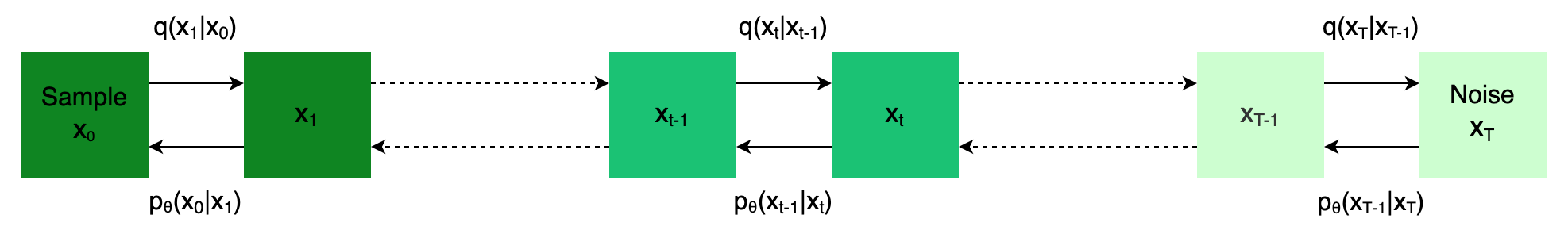
Figure 1: Denoising diffusion model

The forward process.

The forward process transforms a datapoint $\mathbf{x}_{0}\sim\mu$ into a noise distribution $q(\mathbf{x}_{T}|\mathbf{x}_{0})$, via a sequence of conditional distributions $q(\mathbf{x}_{t}|\mathbf{x}_{t-1})$ for $1\leq t\leq T$. It is assumed that the forward process is defined so that for large enough $T$, the distribution $q(\mathbf{x}_{T}|\mathbf{x}_{0})$ is close to a simple noise distribution referred to as the prior distribution $p(\mathbf{x}_{T})$. For instance, Ho et al. (2020) chose $p(\mathbf{x}_{T})=\mathcal{N}\left(\mathbf{x}_{T};\mathbf{0},\mathbf{I}\right)$, the standard normal distribution.

The backward process.

The backward process is a Markov process with parametric transition kernels. The goal of the backward process is to implement the reverse action of the forward process: transforming noise samples into (approximate) samples from distribution $\mu$. Following Ho et al. (2020), we assume the backward process to be defined by Gaussian distributions $p_{\theta}(\mathbf{x}_{t-1}|\mathbf{x}_{t})$ defined for $2\leq t\leq T$ as

$$p_{\theta}(\mathbf{x}_{t-1}|\mathbf{x}_{t})=\mathcal{N}\left(\mathbf{x}_{t-1};g_{\theta}^{t}(\mathbf{x}_{t}),\sigma_{t}^{2}\mathbf{I}\right),$$ (1)

and

$$p_{\theta}(\mathbf{x}_{0}|\mathbf{x}_{1})=g_{\theta}^{1}(\mathbf{x}_{1}),$$ (2)

where the variance parameters $\sigma_{t}\in_{\geq 0}$ are defined by a fixed schedule, the mean functions $g_{\theta}^{t}:^{D}\rightarrow^{D}$ are learned using a neural network for $2\leq t\leq T$, and $g_{\theta}^{1}:^{D}\rightarrow\mathcal{X}$ is a separate function dependent on $\sigma_{1}$. In practice, Ho et al. (2020) used the same network for the functions $g_{\theta}^{t}$ for $2\leq t\leq T$, and a separate discrete decoder for $g_{\theta}^{1}$.

Generating new samples from a trained diffusion model is done by sampling $\mathbf{x}_{t-1}\sim p_{\theta}(\mathbf{x}_{t-1}|\mathbf{x}_{t})$ for $1\leq t\leq T$, starting from a noise vector $\mathbf{x}_{T}\sim p(\mathbf{x}_{T})$ sampled from the prior $p(\mathbf{x}_{T})$.

We make the following assumption on the backward process.

Assumption 1.

We assume for each $1\leq t\leq T$ there exists a constant $K_{\theta}^{t}>0$ such that for every $\mathbf{x}_{1},\mathbf{x}_{2}\in\mathcal{X}$,

$$\left\lVert g_{\theta}^{t}(\mathbf{x}_{1})-g_{\theta}^{t}(\mathbf{x}_{2})\right\rVert\leq K_{\theta}^{t}\left\lVert\mathbf{x}_{1}-\mathbf{x}_{2}\right\rVert.$$

In other words, $g_{\theta}^{t}$ is $K_{\theta}^{t}$-Lipschitz continuous. We discuss this assumption in Remark 3.2.

2.2 Additional Definitions

We define the distribution $\pi_{\theta}(\cdot|\mathbf{x}_{0})$ as

$$\pi_{\theta}(\cdot|\mathbf{x}_{0})=q(\mathbf{x}_{T}|\mathbf{x}_{0})p_{\theta}(\mathbf{x}_{T-1}|\mathbf{x}_{T})p_{\theta}(\mathbf{x}_{T-2}|\mathbf{x}_{T-1})\dots p_{\theta}(\mathbf{x}_{1}|\mathbf{x}_{2})p_{\theta}(\cdot|\mathbf{x}_{1}).$$ (3)

Intuitively, for each $\mathbf{x}_{0}\in\mathcal{X}$, $\pi_{\theta}(\cdot|\mathbf{x}_{0})$ denotes the distribution on $\mathcal{X}$ obtained by reconstructing samples from $q(\mathbf{x}_{T}|\mathbf{x}_{0})$ through the backward process. Another way of seeing this distribution is that for any function $f:\mathcal{X}\rightarrow$, the following equation holds:

$$\operatorname*{\mathbb{E}}_{\pi_{\theta}(\hat{\mathbf{x}}_{0}|\mathbf{x}_{0})}f(\hat{\mathbf{x}}_{0})=\operatorname*{\mathbb{E}}_{q(\mathbf{x}_{T}|\mathbf{x}_{0})}\operatorname*{\mathbb{E}}_{p_{\theta}(\mathbf{x}_{T-1}|\mathbf{x}_{T})}\dots\operatorname*{\mathbb{E}}_{p_{\theta}(\mathbf{x}_{1}|\mathbf{x}_{2})}\operatorname*{\mathbb{E}}_{p_{\theta}(\hat{\mathbf{x}}_{0}|\mathbf{x}_{1})}f(\hat{\mathbf{x}}_{0}).$$ (4)

Given a finite set $S=\{\mathbf{x}_{0}^{1},\dots,\mathbf{x}_{0}^{n}\}\stackrel{{\scriptstyle\textrm{{iid}}}}{{\sim}}\mu$, we define the regenerated distribution as the following mixture of measures:

$$\mu_{\theta}^{n}=\frac{1}{n}\sum_{i=1}^{n}{\pi_{\theta}(\cdot|\mathbf{x}_{0}^{i})}.$$ (5)

This definition is analogous to the empirical regenerated distribution defined by Mbacke et al. (2023) for VAEs. The distribution on $\mathcal{X}$ learned by the diffusion model is denoted $\pi_{\theta}(\cdot)$ and defined as

$$\pi_{\theta}(\cdot)=p(\mathbf{x}_{T})p_{\theta}(\mathbf{x}_{T-1}|\mathbf{x}_{T})p_{\theta}(\mathbf{x}_{T-2}|\mathbf{x}_{T-1})\dots p_{\theta}(\mathbf{x}_{1}|\mathbf{x}_{2})p_{\theta}(\cdot|\mathbf{x}_{1}).$$

In other words, for any function $f:\mathcal{X}\rightarrow$, the expectation of $f$ w.r.t. $\pi_{\theta}(\cdot)$ is

$$\operatorname*{\mathbb{E}}_{\pi_{\theta}(\hat{\mathbf{x}}_{0})}f(\hat{\mathbf{x}}_{0})=\operatorname*{\mathbb{E}}_{p(\mathbf{x}_{T})}\operatorname*{\mathbb{E}}_{p_{\theta}(\mathbf{x}_{T-1}|\mathbf{x}_{T})}\dots\operatorname*{\mathbb{E}}_{p_{\theta}(\mathbf{x}_{1}|\mathbf{x}_{2})}\operatorname*{\mathbb{E}}_{p_{\theta}(\hat{\mathbf{x}}_{0}|\mathbf{x}_{1})}f(\hat{\mathbf{x}}_{0}).$$

Hence, both $\pi_{\theta}(\cdot)$ and $\pi_{\theta}(\cdot|\mathbf{x}_{0})$ are defined using the backward process, with the difference that $\pi_{\theta}(\cdot)$ starts with the prior $p(\mathbf{x}_{T})=\mathcal{N}\left(\mathbf{x}_{T};\mathbf{0},\mathbf{I}\right)$ while $\pi_{\theta}(\cdot|\mathbf{x}_{0})$ starts with the noise distribution $q(\mathbf{x}_{T}|\mathbf{x}_{0})$.

Finally, we define the loss function $\ell^{\theta}:\mathcal{X}\times\mathcal{X}\rightarrow$ as

$$\ell^{\theta}(\mathbf{x}_{T},\mathbf{x}_{0})=\operatorname*{\mathbb{E}}_{p_{\theta}(\mathbf{x}_{T-1}|\mathbf{x}_{T})}\operatorname*{\mathbb{E}}_{p_{\theta}(\mathbf{x}_{T-2}|\mathbf{x}_{T-1})}\dots\operatorname*{\mathbb{E}}_{p_{\theta}(\mathbf{x}_{1}|\mathbf{x}_{2})}\operatorname*{\mathbb{E}}_{p_{\theta}(\hat{\mathbf{x}}_{0}|\mathbf{x}_{1})}\left\lVert\mathbf{x}_{0}-\hat{\mathbf{x}}_{0}\right\rVert.$$ (6)

Hence, given a noise vector $\mathbf{x}_{T}$ and a sample $\mathbf{x}_{0}$, the loss $\ell^{\theta}(\mathbf{x}_{T},\mathbf{x}_{0})$ denotes the average Euclidean distance between $\mathbf{x}_{0}$ and any sample obtained by passing $\mathbf{x}_{T}$ through the backward process.

2.3 Our Approach

The goal is to upper-bound the distance $W_{1}(\mu,\pi_{\theta}(\cdot))$. Since the triangle inequality implies

$$W_{1}(\mu,\pi_{\theta}(\cdot))\leq W_{1}(\mu,\mu_{\theta}^{n})+W_{1}(\mu_{\theta}^{n},\pi_{\theta}(\cdot)),$$ (7)

we can upper-bound the distance $W_{1}(\mu,\pi_{\theta}(\cdot))$ by upper-bounding the two expressions on the right-hand side of equation 7 separately. The upper bound on $W_{1}(\mu,\mu_{\theta}^{n})$ is obtained using a straightforward adaptation of a proof by Mbacke et al. (2023). First, $W_{1}(\mu,\mu_{\theta}^{n})$ is upper-bounded using the expectation of the loss function $\ell^{\theta}$, then the resulting expression is upper-bounded using a PAC-Bayesian-style expression dependent on the empirical risk and the prior-matching term.

The upper bound on the second term $W_{1}(\mu_{\theta}^{n},\pi_{\theta}(\cdot))$ uses the definition of $\mu_{\theta}^{n}$. Intuitively, the difference between $\pi_{\theta}(\cdot|\mathbf{x}_{0}^{i})$ and $\pi_{\theta}(\cdot)$ is determined by the corresponding initial distributions: $q(\mathbf{x}_{T}|\mathbf{x}_{0}^{i})$ for $\pi_{\theta}(\cdot|\mathbf{x}_{0}^{i})$, and $p(\mathbf{x}_{T})$ for $\pi_{\theta}(\cdot)$. Hence, if the two initial distributions are close and if the steps of the backward process are smooth (see Assumption 1), then $\pi_{\theta}(\cdot|\mathbf{x}_{0}^{i})$ and $\pi_{\theta}(\cdot)$ are close to each other.

3 Main Result

3.1 Theorem Statement

We are now ready to state our main result: a quantitative upper bound on the Wasserstein distance between the data-generating distribution $\mu$ and the learned distribution $\pi_{\theta}(\cdot)$.

Theorem 3.1.

Assume the instance space $\mathcal{X}$ has finite diameter $\Delta=\sup_{\mathbf{x},\mathbf{x}^{\prime}\in\mathcal{X}}\left\lVert\mathbf{x}-\mathbf{x}^{\prime}\right\rVert<\infty$, and let $\lambda>0$ and $\delta\in(0,1)$ be real numbers. Using the definitions and assumptions of the previous section, the following inequality holds with probability at least $1-\delta$ over the random draw of $S=\{\mathbf{x}_{0}^{1},\dots,\mathbf{x}_{0}^{n}\}\stackrel{{\scriptstyle\textrm{{iid}}}}{{\sim}}\mu$:

$$\begin{split}W_{1}(\mu,\pi_{\theta}(\cdot))\leq\frac{1}{n}\sum_{i=1}^{n}{\left\{\operatorname*{\mathbb{E}}_{q(\mathbf{x}_{T}|\mathbf{x}_{0}^{i})}\ell^{\theta}(\mathbf{x}_{T},\mathbf{x}_{0}^{i})\right\}}+\frac{1}{\lambda}\left[\sum_{i=1}^{n}{\mathrm{KL}(q(\mathbf{x}_{T}|\mathbf{x}_{0}^{i})\,||\,p(\mathbf{x}_{T}))}+\log\frac{1}{\delta}\right]+\frac{\lambda\Delta^{2}}{8n}+\\ \left(\prod_{t=1}^{T}{K_{\theta}^{t}}\right)\frac{1}{n}\sum_{i=1}^{n}{\left\{\operatorname*{\mathbb{E}}_{q(\mathbf{x}_{T}|\mathbf{x}_{0}^{i})}\operatorname*{\mathbb{E}}_{p(\mathbf{y}_{T})}\left\lVert\mathbf{x}_{T}-\mathbf{y}_{T}\right\rVert\right\}}+\left(\sum_{t=2}^{T}{\left(\prod_{i=1}^{t-1}{K_{i}}\right)\sigma_{t}}\right)\operatorname*{\mathbb{E}}_{\bm{\epsilon},\bm{\epsilon}^{\prime}}\left\lVert\bm{\epsilon}-\bm{\epsilon}^{\prime}\right\rVert,\end{split}$$ (8)

where $\bm{\epsilon},\bm{\epsilon}^{\prime}\sim\mathcal{N}\left(\mathbf{0},\mathbf{I}\right)$.

Remark 3.1.

Before presenting the proof, let us discuss Theorem 3.1.

• Because the right-hand side of equation 8 depends on a quantity computed using a finite i.i.d.  sample $S$, the bound holds with high probability w.r.t. the randomness of $S$. This is the price we pay for having quantitative upper bounds with no exponential dependencies and no assumptions on the data-generating distribution $\mu$.

• The first term on the right-hand side of equation 8 is the average reconstruction loss computed on $S=\{\mathbf{x}_{0}^{1},\dots,\mathbf{x}_{0}^{n}\}$. Note that for each $1\leq i\leq n$, the expectation of $\ell^{\theta}(\mathbf{x}_{T}|\mathbf{x}_{0}^{i})$ is only computed w.r.t. the noise distribution $q(\mathbf{x}_{T}|\mathbf{x}_{0}^{i})$ defined by $\mathbf{x}_{0}^{i}$ itself. Hence, this term measures how well a noise vector $\mathbf{x}_{T}\sim q(\mathbf{x}_{T}|\mathbf{x}_{0}^{i})$ recovers the original sample $\mathbf{x}_{0}^{i}$ using the backward process and averages over $S=\{\mathbf{x}_{0}^{1},\dots,\mathbf{x}_{0}^{n}\}$.

• If the Lipschitz constants satisfy $K_{\theta}^{t}<1$ for $1\leq t\leq T$, then the larger $T$ is, the smaller the upper bound gets because the product of $K_{\theta}^{t}$’s converges to $0$. In Remark 3.2, we show that the assumption that $K_{\theta}^{t}<1$ for all $t$ is a quite reasonable one.

• The hyperparameter $\lambda$ controls the trade-off between the prior-matching term and the diameter term $\frac{\Delta^{2}}{8n}$. If $K_{\theta}^{t}<1$ for all $1\leq t\leq T$ and $T\rightarrow\infty$, then the convergence of the bound largely depends on the choice of $\lambda$. In that case, $\lambda\propto n^{2}$ leads to a faster convergence, while $\lambda\propto n$ leads to a slower convergence to a smaller quantity.

3.2 Proof of the main theorem

The following result is an adaptation of a result by Mbacke et al. (2023).

Lemma 3.2.

Let $\lambda>0$ and $\delta\in(0,1)$ be real numbers. With probability at least $1-\delta$ over the randomness of $S=\{\mathbf{x}_{0}^{1},\dots,\mathbf{x}_{0}^{n}\}\stackrel{{\scriptstyle\textrm{{iid}}}}{{\sim}}\mu$, the following holds

$$\begin{split}W_{1}(\mu,\mu_{\theta}^{n})\leq\frac{1}{n}\sum_{i=1}^{n}{\left\{\operatorname*{\mathbb{E}}_{q(\mathbf{x}_{T}|\mathbf{x}_{0}^{i})}\ell^{\theta}(\mathbf{x}_{T},\mathbf{x}_{0}^{i})\right\}}+\frac{1}{\lambda}\left[\sum_{i=1}^{n}{\mathrm{KL}(q(\mathbf{x}_{T}|\mathbf{x}_{0}^{i})\,||\,p(\mathbf{x}_{T}))}+\log\frac{1}{\delta}\right]+\frac{\lambda\Delta^{2}}{8n}.\end{split}$$ (9)

The proof of this result is a straightforward adaptation of Mbacke et al. (2023, Lemma D.1). We provide the proof in the supplementary material (Section A.1) for completeness.

Now, let us focus our attention on the second term of the right-hand side of equation 7, namely $W_{1}(\mu_{\theta}^{n},\pi_{\theta}(\cdot))$. This part is trickier than for VAEs, for which the generative model’s distribution is simply a pushforward measure. Here, we have a non-deterministic sampling process with $T$ steps.

Assumption 1 leads to the following lemma on the backward process.

Lemma 3.3.

For any given $\mathbf{x}_{1},\mathbf{y}_{1}\in\mathcal{X}$ we have

$$\operatorname*{\mathbb{E}}_{p_{\theta}(\mathbf{x}_{0}|\mathbf{x}_{1})}\operatorname*{\mathbb{E}}_{p_{\theta}(\mathbf{y}_{0}|\mathbf{y}_{1})}\left\lVert\mathbf{x}_{0}-\mathbf{y}_{0}\right\rVert\leq K_{1}\left\lVert\mathbf{x}_{1}-\mathbf{y}_{1}\right\rVert.$$

Moreover, if $2\leq t\leq T$, then for any given $\mathbf{x}_{t},\mathbf{y}_{t}\in\mathcal{X}$ we have

$$\operatorname*{\mathbb{E}}_{p_{\theta}(\mathbf{x}_{t-1}|\mathbf{x}_{t})}\operatorname*{\mathbb{E}}_{p_{\theta}(\mathbf{y}_{t-1}|\mathbf{y}_{t})}\left\lVert\mathbf{x}_{t-1}-\mathbf{y}_{t-1}\right\rVert\leq K_{\theta}^{t}\left\lVert\mathbf{x}_{t}-\mathbf{y}_{t}\right\rVert+\sigma_{t}\operatorname*{\mathbb{E}}_{\bm{\epsilon},\bm{\epsilon}^{\prime}}\left\lVert\bm{\epsilon}-\bm{\epsilon}^{\prime}\right\rVert,$$

where $\bm{\epsilon},\bm{\epsilon}^{\prime}\sim\mathcal{N}\left(\mathbf{0},\mathbf{I}\right)$, meaning $\operatorname*{\mathbb{E}}_{\bm{\epsilon},\bm{\epsilon}^{\prime}}$ is a shorthand for $\operatorname*{\mathbb{E}}_{\bm{\epsilon},\bm{\epsilon}^{\prime}\sim\mathcal{N}\left(\mathbf{0},\mathbf{I}\right)}$.

Proof.

For the first part, let $\mathbf{x}_{1},\mathbf{y}_{1}\in\mathcal{X}$. Since according to equation 2 $p_{\theta}(\mathbf{x}_{0}|\mathbf{x}_{1})=\delta_{g_{\theta}^{1}(\mathbf{x}_{1})}(\mathbf{x}_{0})$ and $p_{\theta}(\mathbf{y}_{0}|\mathbf{y}_{1})=\delta_{g_{\theta}^{1}(\mathbf{y}_{1})}(\mathbf{y}_{0})$, we have

$$\operatorname*{\mathbb{E}}_{p_{\theta}(\mathbf{x}_{0}|\mathbf{x}_{1})}\operatorname*{\mathbb{E}}_{p_{\theta}(\mathbf{y}_{0}|\mathbf{y}_{1})}\left\lVert\mathbf{x}_{0}-\mathbf{y}_{0}\right\rVert=\left\lVert g_{\theta}^{1}(\mathbf{x}_{1})-g_{\theta}^{1}(\mathbf{y}_{1})\right\rVert\leq K_{1}\left\lVert\mathbf{x}_{1}-\mathbf{y}_{1}\right\rVert.$$

For the second part, let $2\leq t\leq T$ and $\mathbf{x}_{t},\mathbf{y}_{t}\in\mathcal{X}$. Since $p_{\theta}(\mathbf{x}_{t-1}|\mathbf{x}_{t})=\mathcal{N}\left(\mathbf{x}_{t-1};g_{\theta}^{t}(\mathbf{x}_{t}),\sigma_{t}^{2}\mathbf{I}\right)$ the reparameterization trick (Kingma & Welling, 2014) implies that sampling

$$\mathbf{x}_{t-1}\sim p_{\theta}(\mathbf{x}_{t-1}|\mathbf{x}_{t})$$

is equivalent to setting

$$\mathbf{x}_{t-1}=g_{\theta}^{t}(\mathbf{x}_{t})+\sigma_{t}\bm{\epsilon}_{t},\quad\text{ with }\bm{\epsilon}_{t}\sim\mathcal{N}\left(\mathbf{0},\mathbf{I}\right).$$ (10)

Using equation 10, the triangle inequality, and Assumption 1, we obtain

$$\begin{split}\operatorname*{\mathbb{E}}_{p_{\theta}(\mathbf{x}_{t-1}|\mathbf{x}_{t})}\operatorname*{\mathbb{E}}_{p_{\theta}(\mathbf{y}_{t-1}|\mathbf{y}_{t})}\left\lVert\mathbf{x}_{t-1}-\mathbf{y}_{t-1}\right\rVert&=\operatorname*{\mathbb{E}}_{\bm{\epsilon}_{t}}\operatorname*{\mathbb{E}}_{\bm{\epsilon}_{t}^{\prime}}\left\lVert g_{\theta}^{t}(\mathbf{x}_{t})+\sigma_{t}\bm{\epsilon}_{t}-g_{\theta}^{t}(\mathbf{y}_{t})-\sigma_{t}\bm{\epsilon}_{t}^{\prime}\right\rVert\\ &\leq\operatorname*{\mathbb{E}}_{\bm{\epsilon}_{t}}\operatorname*{\mathbb{E}}_{\bm{\epsilon}_{t}^{\prime}}\left\lVert g_{\theta}^{t}(\mathbf{x}_{t})-g_{\theta}^{t}(\mathbf{y}_{t})\right\rVert+\sigma_{t}\operatorname*{\mathbb{E}}_{\bm{\epsilon}_{t}}\operatorname*{\mathbb{E}}_{\bm{\epsilon}_{t}^{\prime}}\left\lVert\bm{\epsilon}_{t}-\bm{\epsilon}_{t}^{\prime}\right\rVert\\ &=\left\lVert g_{\theta}^{t}(\mathbf{x}_{t})-g_{\theta}^{t}(\mathbf{y}_{t})\right\rVert+\sigma_{t}\operatorname*{\mathbb{E}}_{\bm{\epsilon}_{t}}\operatorname*{\mathbb{E}}_{\bm{\epsilon}_{t}^{\prime}}\left\lVert\bm{\epsilon}_{t}-\bm{\epsilon}_{t}^{\prime}\right\rVert\\ &\leq K_{\theta}^{t}\left\lVert\mathbf{x}_{t}-\mathbf{y}_{t}\right\rVert+\sigma_{t}\operatorname*{\mathbb{E}}_{\bm{\epsilon}}\operatorname*{\mathbb{E}}_{\bm{\epsilon}^{\prime}}\left\lVert\bm{\epsilon}-\bm{\epsilon}^{\prime}\right\rVert,\end{split}$$

where $\bm{\epsilon},\bm{\epsilon}^{\prime}\sim\mathcal{N}\left(\mathbf{0},\mathbf{I}\right)$. ∎

Next, we can use the inequalities of Lemma 3.3, to prove the following result.

Lemma 3.4.

Let $T\geq 1$. The following inequality holds.

$$\begin{split}\operatorname*{\mathbb{E}}_{p_{\theta}(\mathbf{x}_{T-1}|\mathbf{x}_{T})}\operatorname*{\mathbb{E}}_{p_{\theta}(\mathbf{y}_{T-1}|\mathbf{y}_{T})}\operatorname*{\mathbb{E}}_{p_{\theta}(\mathbf{x}_{T-2}|\mathbf{x}_{T-1})}\operatorname*{\mathbb{E}}_{p_{\theta}(\mathbf{y}_{T-2}|\mathbf{y}_{T-1})}\dots\operatorname*{\mathbb{E}}_{p_{\theta}(\mathbf{x}_{0}|\mathbf{x}_{1})}\operatorname*{\mathbb{E}}_{p_{\theta}(\mathbf{y}_{0}|\mathbf{y}_{1})}\left\lVert\mathbf{x}_{0}-\mathbf{y}_{0}\right\rVert\leq\\ \left(\prod_{t=1}^{T}{K_{\theta}^{t}}\right)\left\lVert\mathbf{x}_{T}-\mathbf{y}_{T}\right\rVert+\left(\sum_{t=2}^{T}{\left(\prod_{i=1}^{t-1}{K_{i}}\right)\sigma_{t}}\right)\operatorname*{\mathbb{E}}_{\bm{\epsilon},\bm{\epsilon}^{\prime}}\left[\left\lVert\bm{\epsilon}-\bm{\epsilon}^{\prime}\right\rVert\right],\end{split}$$

where $\bm{\epsilon},\bm{\epsilon}^{\prime}\sim\mathcal{N}\left(\mathbf{0},\mathbf{I}\right)$.

Proof Idea.

Lemma 3.4 is proven by induction using Lemma 3.3 in the induction step. The details are in the supplementary material (Section A.2). ∎

Using the two previous lemmas, we obtain the following upper bound on $W_{1}(\mu_{\theta}^{n},\pi_{\theta}(\cdot))$.

Lemma 3.5.

The following inequality holds

$$W_{1}(\mu_{\theta}^{n},\pi_{\theta}(\cdot))\leq\left(\prod_{t=1}^{T}{K_{\theta}^{t}}\right)\frac{1}{n}\sum_{i=1}^{n}{\left\{\operatorname*{\mathbb{E}}_{q(\mathbf{x}_{T}|\mathbf{x}_{0}^{i})}\operatorname*{\mathbb{E}}_{p(\mathbf{y}_{T})}\left\lVert\mathbf{x}_{T}-\mathbf{y}_{T}\right\rVert\right\}}+\left(\sum_{t=2}^{T}{\left(\prod_{i=1}^{t-1}{K_{i}}\right)\sigma_{t}}\right)\operatorname*{\mathbb{E}}_{\bm{\epsilon},\bm{\epsilon}^{\prime}}\left\lVert\bm{\epsilon}-\bm{\epsilon}^{\prime}\right\rVert,$$

where $\bm{\epsilon},\bm{\epsilon}^{\prime}\sim\mathcal{N}\left(\mathbf{0},\mathbf{I}\right)$.

Proof.

Using the definition of $W_{1}$, the trivial coupling, the definitions of $\mu_{\theta}^{n}$ and $\pi_{\theta}(\cdot)$, and Lemma 3.4, we get

$$\begin{split}W_{1}(\mu_{\theta}^{n},\pi_{\theta}{(\cdot)})&=\inf_{\pi\in\Gamma(\mu_{\theta}^{n},\pi_{\theta}{(\cdot)})}\int d(\mathbf{x},\mathbf{y})\,d\pi(\mathbf{x},\mathbf{y})\\ &\leq\operatorname*{\mathbb{E}}_{\mathbf{x}\sim\mu_{\theta}^{n}}\operatorname*{\mathbb{E}}_{\mathbf{y}\sim\pi_{\theta}{(\mathbf{y})}}\left[\left\lVert\mathbf{x}-\mathbf{y}\right\rVert\right]\\ &=\frac{1}{n}\sum_{i=1}^{n}{\left\{\operatorname*{\mathbb{E}}_{q(\mathbf{x}_{T}|\mathbf{x}_{0}^{i})}\operatorname*{\mathbb{E}}_{p(\mathbf{y}_{T})}\operatorname*{\mathbb{E}}_{p_{\theta}(\mathbf{x}_{T-1}|\mathbf{x}_{T})}\operatorname*{\mathbb{E}}_{p_{\theta}(\mathbf{y}_{T-1}|\mathbf{y}_{T})}\dots\operatorname*{\mathbb{E}}_{p_{\theta}(\mathbf{x}_{0}|\mathbf{x}_{1})}\operatorname*{\mathbb{E}}_{p_{\theta}(\mathbf{y}_{0}|\mathbf{y}_{1})}\left\lVert\mathbf{x}_{0}-\mathbf{y}_{0}\right\rVert\right\}}\\[4.2679pt] &\leq\frac{1}{n}\sum_{i=1}^{n}{\left\{\operatorname*{\mathbb{E}}_{q(\mathbf{x}_{T}|\mathbf{x}_{0}^{i})}\operatorname*{\mathbb{E}}_{p(\mathbf{y}_{T})}\left[\left(\prod_{t=1}^{T}{K_{\theta}^{t}}\right)\left\lVert\mathbf{x}_{T}-\mathbf{y}_{T}\right\rVert+\left(\sum_{t=2}^{T}{\left(\prod_{j=1}^{t-1}{K_{j}}\right)\sigma_{t}}\right)\operatorname*{\mathbb{E}}_{\bm{\epsilon},\bm{\epsilon}^{\prime}}\left[\left\lVert\bm{\epsilon}-\bm{\epsilon}^{\prime}\right\rVert\right]\right]\right\}}\\[4.2679pt] &=\left(\prod_{t=1}^{T}{K_{\theta}^{t}}\right)\frac{1}{n}\sum_{i=1}^{n}{\left\{\operatorname*{\mathbb{E}}_{q(\mathbf{x}_{T}|\mathbf{x}_{0}^{i})}\operatorname*{\mathbb{E}}_{p(\mathbf{y}_{T})}\left\lVert\mathbf{x}_{T}-\mathbf{y}_{T}\right\rVert\right\}}+\left(\sum_{t=2}^{T}{\left(\prod_{i=1}^{t-1}{K_{i}}\right)\sigma_{t}}\right)\operatorname*{\mathbb{E}}_{\bm{\epsilon},\bm{\epsilon}^{\prime}}\left\lVert\bm{\epsilon}-\bm{\epsilon}^{\prime}\right\rVert\end{split}$$

∎

Combining Lemmas 3.2 and 3.5 with equation 7 yields Theorem 3.1 .

3.3 Special case using the forward process of Ho et al. (2020)

Note that the general theorem holds for any forward process, as long as the backward process satisfies Assumption 1. Now, we give the statement of the theorem in the special case of the forward process defined by Ho et al. (2020).

Let $\mathcal{X}\subseteq^{D}$. In Ho et al. (2020), the forward process is a Gauss-Markov process defined as

$$q(\mathbf{x}_{t}|\mathbf{x}_{t-1})=\mathcal{N}\left(\mathbf{x}_{t};\sqrt{\alpha_{t}}\mathbf{x}_{t},(1-\alpha_{t})\mathbf{I}\right),$$

where $\alpha_{1},\dots,\alpha_{T}$ is a fixed noise schedule such that $0<\alpha_{t}<1$ for all $t$. This definition implies that for each $1\leq t\leq T$,

$$q(\mathbf{x}_{t}|\mathbf{x}_{0})=\mathcal{N}\left(\mathbf{x}_{t};\sqrt{\bar{\alpha}_{t}}\mathbf{x}_{0},(1-\bar{\alpha}_{t}\mathbf{I})\right),\quad\text{ with }\bar{\alpha_{t}}=\prod_{i=1}^{t}{\alpha_{i}}.$$

Now, we discuss Assumption 1 under these definitions.

Remark 3.2.

We can get a glimpse at the range of $K_{\theta}^{t}$ for a trained DDPM by looking at the distribution $q(\mathbf{x}_{t-1}|\mathbf{x}_{t},\mathbf{x}_{0})$, since $p_{\theta}(\mathbf{x}_{t-1}|\mathbf{x}_{t})$ is optimized to be as close as possible to $q(\mathbf{x}_{t-1}|\mathbf{x}_{t},\mathbf{x}_{0})$. Ho et al. (2020) showed that

$$q(\mathbf{x}_{t-1}|\mathbf{x}_{t},\mathbf{x}_{0})=\mathcal{N}\left(\mathbf{x}_{t-1};\mu_{q}^{t}(\mathbf{x}_{t},\mathbf{x}_{0}),\sigma_{t}^{2}\mathbf{I}\right),$$

where

$$\mu_{q}^{t}(\mathbf{x}_{t},\mathbf{x}_{0})=\frac{\sqrt{\alpha_{t}}(1-\bar{\alpha}_{t-1})}{1-\bar{\alpha}_{t}}\mathbf{x}_{t}+\frac{\sqrt{\bar{\alpha}_{t-1}}(1-\alpha_{t})}{1-\bar{\alpha}_{t}}\mathbf{x}_{0}.$$ (11)

For a given $\mathbf{x}_{0}\sim\mu$, let us take a look at the Lipschitz norm of $\mathbf{x}\mapsto\mu_{q}^{t}(\mathbf{x},\mathbf{x}_{0})$. Using equation 11, we have

$$\mu_{q}^{t}(\mathbf{x}_{t},\mathbf{x}_{0})-\mu_{q}^{t}(\mathbf{y}_{t},\mathbf{x}_{0})=\frac{\sqrt{\alpha_{t}}(1-\bar{\alpha}_{t-1})}{1-\bar{\alpha}_{t}}(\mathbf{x}_{t}-\mathbf{y}_{t}).$$

Hence, $\mathbf{x}\mapsto\mu_{q}^{t}(\mathbf{x},\mathbf{x}_{0})$ is $K^{\prime}_{t}$-Lipschitz continuous with

$$K^{\prime}_{t}=\frac{\sqrt{\alpha_{t}}(1-\bar{\alpha}_{t-1})}{1-\bar{\alpha}_{t}}.$$

Now, if for all $1\leq t\leq T$, $\alpha_{t}<1$, then we have $1-\bar{\alpha}_{t}>1-\bar{\alpha}_{t-1}$ which implies $K^{\prime}_{t}<1$ for all $1\leq t\leq T$.

The prior-matching term.

With the definitions of this section, the prior matching term $\mathrm{KL}(q(\mathbf{x}_{T}|\mathbf{x}_{0})\,||\,p(\mathbf{x}_{T}))$ has the following closed form:

$$\mathrm{KL}(q(\mathbf{x}_{T}|\mathbf{x}_{0})\,||\,p(\mathbf{x}_{T}))=\frac{1}{2}\left[-D\log(1-\bar{\alpha}_{T})-D\bar{\alpha}_{T}+\bar{\alpha}_{T}\left\lVert\mathbf{x}_{0}\right\rVert^{2}\right].$$

Upper-bounds on the average distance between Gaussian vectors.

If $\bm{\epsilon},\bm{\epsilon}^{\prime}$ are $D$-dimensional vectors sampled from $\mathcal{N}\left(\mathbf{0},\mathbf{I}\right)$, then

$$\operatorname*{\mathbb{E}}_{\bm{\epsilon},\bm{\epsilon}^{\prime}}\left\lVert\bm{\epsilon}-\bm{\epsilon}^{\prime}\right\rVert\leq\sqrt{2D}.$$

Moreover, since $q(\mathbf{x}_{T}|\mathbf{x}_{0}^{i})=\mathcal{N}\left(\mathbf{x}_{T};\bar{\alpha}_{T}\mathbf{x}_{0}^{i},(1-\bar{\alpha}_{T})\mathbf{I}\right)$ and the prior $p(\mathbf{y}_{T})=\mathcal{N}\left(\mathbf{y}_{T};\mathbf{0},\mathbf{I}\right)$,

$$\operatorname*{\mathbb{E}}_{q(\mathbf{x}_{T}|\mathbf{x}_{0}^{i})}\operatorname*{\mathbb{E}}_{p(\mathbf{y}_{T})}\left\lVert\mathbf{x}_{T}-\mathbf{y}_{T}\right\rVert\leq\sqrt{\bar{\alpha}_{T}\left\lVert\mathbf{x}_{0}^{i}\right\rVert^{2}+(2-\bar{\alpha}_{T})D}.$$

Special case of the main theorem.

With the definitions of this section, the inequality of Theorem 3.1 implies that with probability at least $1-\delta$ over the randomness of $\{\mathbf{x}_{0}^{1},\dots,\mathbf{x}_{0}^{n}\}\stackrel{{\scriptstyle\textrm{{iid}}}}{{\sim}}\mu$:

$$\begin{split}W_{1}(\mu,\pi_{\theta}(\cdot))\leq\frac{1}{n}\sum_{i=1}^{n}{\left\{\operatorname*{\mathbb{E}}_{q(\mathbf{x}_{T}|\mathbf{x}_{0}^{i})}\ell^{\theta}(\mathbf{x}_{T},\mathbf{x}_{0}^{i})\right\}}\ +\ \frac{1}{\lambda}\left[\frac{1}{2}\sum_{i=1}^{n}{\left[-D\log(1-\bar{\alpha}_{T})-D\bar{\alpha}_{T}+\bar{\alpha}_{T}\left\lVert\mathbf{x}_{0}^{i}\right\rVert^{2}\right]}+\log\frac{1}{\delta}\right]\ +\ \\ \frac{\lambda\Delta^{2}}{8n}\ +\ \left(\prod_{t=1}^{T}{K_{\theta}^{t}}\right)\frac{1}{n}\sum_{i=1}^{n}{\sqrt{\bar{\alpha}_{T}\left\lVert\mathbf{x}_{0}^{i}\right\rVert^{2}+(2-\bar{\alpha}_{T})D}}\ +\ \sqrt{2D}\left(\sum_{t=2}^{T}{\left(\prod_{i=1}^{t-1}{K_{i}}\right)\sigma_{t}}\right)\,.\end{split}$$

4 Conclusion

This note presents a novel upper bound on the Wasserstein distance between the data-generating distribution and the distribution learned by a diffusion model. Unlike previous works in the field, our main result simultaneously avoids strong assumptions on the data-generating distribution, assumptions on the learned score function, and exponential dependencies, while still providing a quantitative upper bound. However, our bound holds with high probability on the randomness of a finite i.i.d. sample, on which a loss function is computed. Since the loss is a chain of expectations w.r.t. Gaussian distributions, it can either be estimated with high precision or upper bounded using the properties of Gaussian distributions.

Acknowledgments

This research is supported by the Canada CIFAR AI Chair Program, and the NSERC Discovery grant RGPIN-2020- 07223. The authors sincerely thank Pascal Germain for interesting discussions and suggestions. The first author thanks Mathieu Bazinet and Florence Clerc for proof-reading the manuscript.

Appendix A Omitted Proofs

A.1 Proof of Lemma 3.2

Recall Lemma 3.2 states that the following inequality holds with probability $1-\delta$:

$$\begin{split}W_{1}(\mu,\mu_{\theta}^{n})\leq\frac{1}{n}\sum_{i=1}^{n}{\left\{\operatorname*{\mathbb{E}}_{q(\mathbf{x}_{T}|\mathbf{x}_{0}^{i})}\ell^{\theta}(\mathbf{x}_{T},\mathbf{x}_{0}^{i})\right\}}+\frac{1}{\lambda}\left[\sum_{i=1}^{n}{\mathrm{KL}(q(\mathbf{x}_{T}|\mathbf{x}_{0}^{i})\,||\,p(\mathbf{x}_{T}))}+\log\frac{1}{\delta}\right]+\frac{\lambda\Delta^{2}}{8n}.\end{split}$$

Proof of Lemma 3.2.

Using the trivial coupling (product of marginals), the definition of $\mu_{\theta}^{n}$ (equation 5), and the definition of the loss function $\ell^{\theta}$, we get

$$\begin{split}W_{1}(\mu,\mu_{\theta}^{n})&=\inf_{\pi\in\Gamma(\mu,\mu_{\theta}^{n})}\int_{\mathcal{X}\times\mathcal{X}}\left\lVert\mathbf{x}-\mathbf{y}\right\rVert\,d\pi(\mathbf{x},\mathbf{y})\\ &\leq\int_{\mathcal{X}}\int_{\mathcal{X}}\left\lVert\mathbf{x}-\mathbf{y}\right\rVert\,d\mu(\mathbf{x})\,d\mu_{\theta}^{n}(\mathbf{y})\\ &=\operatorname*{\mathbb{E}}_{\mathbf{x}\sim\mu}\operatorname*{\mathbb{E}}_{\mathbf{y}\sim\mu_{\theta}^{n}}\left\lVert\mathbf{x}-\mathbf{y}\right\rVert\\ &=\operatorname*{\mathbb{E}}_{\mathbf{x}\sim\mu}\left[\frac{1}{n}\sum_{i=1}^{n}{\left(\operatorname*{\mathbb{E}}_{q(\mathbf{x}_{T}|\mathbf{x}_{0}^{i})}\operatorname*{\mathbb{E}}_{p_{\theta}(\mathbf{x}_{T-1}|\mathbf{x}_{T})}\dots\operatorname*{\mathbb{E}}_{p_{\theta}(\mathbf{x}_{1}|\mathbf{x}_{2})}\operatorname*{\mathbb{E}}_{p_{\theta}(\mathbf{y}|\mathbf{x}_{1})}\left\lVert\mathbf{x}-\mathbf{y}\right\rVert\right)}\right]\\ &=\operatorname*{\mathbb{E}}_{\mathbf{x}\sim\mu}\left[\frac{1}{n}\sum_{i=1}^{n}{\operatorname*{\mathbb{E}}_{q(\mathbf{x}_{T}|\mathbf{x}_{0}^{i})}\ell^{\theta}(\mathbf{x}_{T},\mathbf{x})}\right].\end{split}$$

Using Mbacke et al. (2023, Lemma B.1), the following inequality holds with probability $1-\delta$:

$$\begin{split}W_{1}(\mu,\mu_{\theta}^{n})\leq\frac{1}{n}\sum_{i=1}^{n}{\left\{\operatorname*{\mathbb{E}}_{q(\mathbf{x}_{T}|\mathbf{x}_{0}^{i})}\ell^{\theta}(\mathbf{x}_{T},\mathbf{x}_{0}^{i})\right\}}+\frac{1}{\lambda}\left[\sum_{i=1}^{n}{\mathrm{KL}(q(\mathbf{x}_{T}|\mathbf{x}_{0}^{i})\,||\,p(\mathbf{x}_{T}))}+\log\frac{1}{\delta}+\right.\\ \left.n\log\operatorname*{\mathbb{E}}_{\mathbf{x}_{0}\sim\mu^{\otimes n}}\operatorname*{\mathbb{E}}_{\mathbf{x}_{T}\sim p(\mathbf{x}_{T})}e^{\lambda\left(\operatorname*{\mathbb{E}}_{\mathbf{y}_{0}\sim\mu}\left[\ell^{\theta}(\mathbf{x}_{T},\mathbf{y}_{0})\right]-\frac{1}{n}\sum_{i=1}^{n}{\ell^{\theta}(\mathbf{x}_{T},\mathbf{x}_{0})}\right)}\right].\end{split}$$ (12)

Now, it remains to upper-bound the exponential moment of equation 9. If $\sup_{\mathbf{x},\mathbf{x}^{\prime}\in\mathcal{X}}\left\lVert\mathbf{x}-\mathbf{x}^{\prime}\right\rVert=\Delta<\infty$, and $\lambda>0$ is a real number, then the definition of the loss function $\ell^{\theta}$ and Hoeffding’s lemma yield

$$n\log\operatorname*{\mathbb{E}}_{\mathbf{x}_{0}\sim\mu}\operatorname*{\mathbb{E}}_{\mathbf{x}_{T}\sim p(\mathbf{x}_{T})}e^{\lambda\left(\operatorname*{\mathbb{E}}_{\mathbf{x}^{\prime}\sim\mu}\left[\ell^{\theta}(\mathbf{x}_{T},\mathbf{x}^{\prime})\right]-\frac{1}{n}\sum_{i=1}^{n}{\ell^{\theta}(\mathbf{x}_{T},\mathbf{x}_{0})}\right)}\leq n\log\textnormal{exp}\left[\frac{\lambda^{2}\Delta^{2}}{8n^{2}}\right]=\frac{\lambda^{2}\Delta^{2}}{8n}.$$

∎

A.2 Proof of Lemma 3.4

Recall Lemma 3.4 states that the following inequality holds:

$$\begin{split}\operatorname*{\mathbb{E}}_{p_{\theta}(\mathbf{x}_{T-1}|\mathbf{x}_{T})}\operatorname*{\mathbb{E}}_{p_{\theta}(\mathbf{y}_{T-1}|\mathbf{y}_{T})}\operatorname*{\mathbb{E}}_{p_{\theta}(\mathbf{x}_{T-2}|\mathbf{x}_{T-1})}\operatorname*{\mathbb{E}}_{p_{\theta}(\mathbf{y}_{T-2}|\mathbf{y}_{T-1})}\dots\operatorname*{\mathbb{E}}_{p_{\theta}(\mathbf{x}_{0}|\mathbf{x}_{1})}\operatorname*{\mathbb{E}}_{p_{\theta}(\mathbf{y}_{0}|\mathbf{y}_{1})}\left\lVert\mathbf{x}_{0}-\mathbf{y}_{0}\right\rVert\leq\\ \left(\prod_{t=1}^{T}{K_{\theta}^{t}}\right)\left\lVert\mathbf{x}_{T}-\mathbf{y}_{T}\right\rVert+\left(\sum_{t=2}^{T}{\left(\prod_{i=1}^{t-1}{K_{i}}\right)\sigma_{t}}\right)\operatorname*{\mathbb{E}}_{\bm{\epsilon},\bm{\epsilon}^{\prime}}\left[\left\lVert\bm{\epsilon}-\bm{\epsilon}^{\prime}\right\rVert\right],\end{split}$$

Proof of Lemma 3.4.

Let’s do a proof by induction on $T$.

• Base case. $T=1$. The inequality becomes

  $$\operatorname*{\mathbb{E}}_{p_{\theta}(\mathbf{x}_{0}|\mathbf{x}_{1})}\operatorname*{\mathbb{E}}_{p_{\theta}(\mathbf{y}_{0}|\mathbf{y}_{1})}\left\lVert\mathbf{x}_{0}-\mathbf{y}_{0}\right\rVert\leq K_{1}\left\lVert\mathbf{x}_{1}-\mathbf{y}_{1}\right\rVert$$ (13)

  which holds by the first part of Lemma 3.3.

• Induction step. Assume $T>1$. The induction hypothesis is

  $$\begin{split}\operatorname*{\mathbb{E}}_{p_{\theta}(\mathbf{x}_{T-2}|\mathbf{x}_{T-1})}\operatorname*{\mathbb{E}}_{p_{\theta}(\mathbf{y}_{T-2}|\mathbf{y}_{T-1})}\dots\operatorname*{\mathbb{E}}_{p_{\theta}(\mathbf{x}_{0}|\mathbf{x}_{1})}\operatorname*{\mathbb{E}}_{p_{\theta}(\mathbf{y}_{0}|\mathbf{y}_{1})}\left\lVert\mathbf{x}_{0}-\mathbf{y}_{0}\right\rVert\leq\\ \left(\prod_{t=1}^{T-1}{K_{\theta}^{t}}\right)\left\lVert\mathbf{x}_{T-1}-\mathbf{y}_{T-1}\right\rVert+\left(\sum_{t=2}^{T-1}{\left(\prod_{i=1}^{t-1}{K_{i}}\right)\sigma_{t}}\right)\operatorname*{\mathbb{E}}_{\bm{\epsilon},\bm{\epsilon}^{\prime}}\left[\left\lVert\bm{\epsilon}-\bm{\epsilon}^{\prime}\right\rVert\right].\end{split}$$ (14)

  Using the induction hypothesis, the linearity of the expectation, Lemma 3.3 with $t:=T$,

  $$\begin{split}&\operatorname*{\mathbb{E}}_{p_{\theta}(\mathbf{x}_{T-1}|\mathbf{x}_{T})}\operatorname*{\mathbb{E}}_{p_{\theta}(\mathbf{y}_{T-1}|\mathbf{y}_{T})}\dots\operatorname*{\mathbb{E}}_{p_{\theta}(\mathbf{x}_{0}|\mathbf{x}_{1})}\operatorname*{\mathbb{E}}_{p_{\theta}(\mathbf{y}_{0}|\mathbf{y}_{1})}\left\lVert\mathbf{x}_{0}-\mathbf{y}_{0}\right\rVert\\ &\leq\operatorname*{\mathbb{E}}_{p_{\theta}(\mathbf{x}_{T-1}|\mathbf{x}_{T})}\operatorname*{\mathbb{E}}_{p_{\theta}(\mathbf{y}_{T-1}|\mathbf{y}_{T})}\left[\left(\prod_{t=1}^{T-1}{K_{\theta}^{t}}\right)\left\lVert\mathbf{x}_{T-1}-\mathbf{y}_{T-1}\right\rVert+\left(\sum_{t=2}^{T-1}{\left(\prod_{i=1}^{t-1}{K_{i}}\right)\sigma_{t}}\right)\operatorname*{\mathbb{E}}_{\bm{\epsilon},\bm{\epsilon}^{\prime}}\left[\left\lVert\bm{\epsilon}-\bm{\epsilon}^{\prime}\right\rVert\right]\right]\\ &=\left(\prod_{t=1}^{T-1}{K_{\theta}^{t}}\right)\operatorname*{\mathbb{E}}_{p_{\theta}(\mathbf{x}_{T-1}|\mathbf{x}_{T})}\operatorname*{\mathbb{E}}_{p_{\theta}(\mathbf{y}_{T-1}|\mathbf{y}_{T})}\left[\left\lVert\mathbf{x}_{T-1}-\mathbf{y}_{T-1}\right\rVert\right]+\left(\sum_{t=2}^{T-1}{\left(\prod_{i=1}^{t-1}{K_{i}}\right)\sigma_{t}}\right)\operatorname*{\mathbb{E}}_{\bm{\epsilon},\bm{\epsilon}^{\prime}}\left[\left\lVert\bm{\epsilon}-\bm{\epsilon}^{\prime}\right\rVert\right]\\ &\leq\left(\prod_{t=1}^{T-1}{K_{\theta}^{t}}\right)\left[K_{\theta}^{t}\left\lVert\mathbf{x}_{T}-\mathbf{y}_{T}\right\rVert+\sigma_{T}\operatorname*{\mathbb{E}}_{\bm{\epsilon},\bm{\epsilon}^{\prime}}\left\lVert\bm{\epsilon}-\bm{\epsilon}^{\prime}\right\rVert\right]+\left(\sum_{t=2}^{T-1}{\left(\prod_{i=1}^{t-1}{K_{i}}\right)\sigma_{t}}\right)\operatorname*{\mathbb{E}}_{\bm{\epsilon},\bm{\epsilon}^{\prime}}\left[\left\lVert\bm{\epsilon}-\bm{\epsilon}^{\prime}\right\rVert\right]\\ &=\left(\prod_{t=1}^{T}{K_{\theta}^{t}}\right)\left\lVert\mathbf{x}_{T}-\mathbf{y}_{T}\right\rVert+\left[\left(\prod_{t=1}^{T-1}{K_{\theta}^{t}}\right)\sigma_{T}+\sum_{t=2}^{T-1}{\left(\prod_{i=1}^{t-1}{K_{i}}\right)\sigma_{t}}\right]\operatorname*{\mathbb{E}}_{\bm{\epsilon},\bm{\epsilon}^{\prime}}\left[\left\lVert\bm{\epsilon}-\bm{\epsilon}^{\prime}\right\rVert\right]\\ &=\left(\prod_{t=1}^{T}{K_{\theta}^{t}}\right)\left\lVert\mathbf{x}_{T}-\mathbf{y}_{T}\right\rVert+\left[\left(\prod_{i=1}^{T-1}{K_{i}}\right)\sigma_{T}+\sum_{t=2}^{T-1}{\left(\prod_{i=1}^{t-1}{K_{i}}\right)\sigma_{t}}\right]\operatorname*{\mathbb{E}}_{\bm{\epsilon},\bm{\epsilon}^{\prime}}\left[\left\lVert\bm{\epsilon}-\bm{\epsilon}^{\prime}\right\rVert\right]\\ &=\left(\prod_{t=1}^{T}{K_{\theta}^{t}}\right)\left\lVert\mathbf{x}_{T}-\mathbf{y}_{T}\right\rVert+\left(\sum_{t=2}^{T}{\left(\prod_{i=1}^{t-1}{K_{i}}\right)\sigma_{t}}\right)\operatorname*{\mathbb{E}}_{\bm{\epsilon},\bm{\epsilon}^{\prime}}\left[\left\lVert\bm{\epsilon}-\bm{\epsilon}^{\prime}\right\rVert\right].\end{split}$$

∎

References

• Block et al. (2020) Adam Block, Youssef Mroueh, and Alexander Rakhlin. Generative modeling with denoising auto-encoders and langevin sampling. arXiv preprint arXiv:2002.00107, 2020.
• Chen et al. (2021) Nanxin Chen, Yu Zhang, Heiga Zen, Ron J Weiss, Mohammad Norouzi, and William Chan. Wavegrad: Estimating gradients for waveform generation. In International Conference on Learning Representations, 2021.
• Chen et al. (2023) Sitan Chen, Sinho Chewi, Jerry Li, Yuanzhi Li, Adil Salim, and Anru Zhang. Sampling is as easy as learning the score: theory for diffusion models with minimal data assumptions. In The Eleventh International Conference on Learning Representations, 2023.
• De Bortoli (2022) Valentin De Bortoli. Convergence of denoising diffusion models under the manifold hypothesis. Transactions on Machine Learning Research, 2022. ISSN 2835-8856.
• De Bortoli et al. (2021) Valentin De Bortoli, James Thornton, Jeremy Heng, and Arnaud Doucet. Diffusion schrödinger bridge with applications to score-based generative modeling. Advances in Neural Information Processing Systems, 34:17695–17709, 2021.
• Dhariwal & Nichol (2021) Prafulla Dhariwal and Alexander Nichol. Diffusion models beat gans on image synthesis. Advances in neural information processing systems, 34:8780–8794, 2021.
• Fefferman et al. (2016) Charles Fefferman, Sanjoy Mitter, and Hariharan Narayanan. Testing the manifold hypothesis. Journal of the American Mathematical Society, 29(4):983–1049, 2016.
• Goodfellow et al. (2014) Ian Goodfellow, Jean Pouget-Abadie, Mehdi Mirza, Bing Xu, David Warde-Farley, Sherjil Ozair, Aaron Courville, and Yoshua Bengio. Generative adversarial nets. In Advances in Neural Information Processing Systems, volume 27, 2014.
• Ho et al. (2020) Jonathan Ho, Ajay Jain, and Pieter Abbeel. Denoising diffusion probabilistic models. Advances in Neural Information Processing Systems, 33:6840–6851, 2020.
• Ho et al. (2022) Jonathan Ho, Chitwan Saharia, William Chan, David J Fleet, Mohammad Norouzi, and Tim Salimans. Cascaded diffusion models for high fidelity image generation. The Journal of Machine Learning Research, 23(1):2249–2281, 2022.
• Hyvärinen & Dayan (2005) Aapo Hyvärinen and Peter Dayan. Estimation of non-normalized statistical models by score matching. Journal of Machine Learning Research, 6(4), 2005.
• Kingma & Welling (2014) Diederik P. Kingma and M. Welling. Auto-encoding variational Bayes. CoRR, abs/1312.6114, 2014.
• Kwon et al. (2022) Dohyun Kwon, Ying Fan, and Kangwook Lee. Score-based generative modeling secretly minimizes the wasserstein distance. Advances in Neural Information Processing Systems, 35:20205–20217, 2022.
• Lee et al. (2022) Holden Lee, Jianfeng Lu, and Yixin Tan. Convergence for score-based generative modeling with polynomial complexity. Advances in Neural Information Processing Systems, 35:22870–22882, 2022.
• Lee et al. (2023) Holden Lee, Jianfeng Lu, and Yixin Tan. Convergence of score-based generative modeling for general data distributions. In International Conference on Algorithmic Learning Theory, pp.  946–985. PMLR, 2023.
• Li et al. (2023) Gen Li, Yuting Wei, Yuxin Chen, and Yuejie Chi. Towards faster non-asymptotic convergence for diffusion-based generative models. arXiv preprint arXiv:2306.09251, 2023.
• Li et al. (2022) Haoying Li, Yifan Yang, Meng Chang, Shiqi Chen, Huajun Feng, Zhihai Xu, Qi Li, and Yueting Chen. Srdiff: Single image super-resolution with diffusion probabilistic models. Neurocomputing, 479:47–59, 2022.
• Luo (2022) Calvin Luo. Understanding diffusion models: A unified perspective. arXiv preprint arXiv:2208.11970, 2022.
• Mbacke et al. (2023) Sokhna Diarra Mbacke, Florence Clerc, and Pascal Germain. Statistical guarantees for variational autoencoders using PAC-bayesian theory. In Thirty-seventh Conference on Neural Information Processing Systems, 2023.
• Narayanan & Mitter (2010) Hariharan Narayanan and Sanjoy Mitter. Sample complexity of testing the manifold hypothesis. Advances in neural information processing systems, 23, 2010.
• Pidstrigach (2022) Jakiw Pidstrigach. Score-based generative models detect manifolds. Advances in Neural Information Processing Systems, 35:35852–35865, 2022.
• Pope et al. (2021) Phil Pope, Chen Zhu, Ahmed Abdelkader, Micah Goldblum, and Tom Goldstein. The intrinsic dimension of images and its impact on learning. In International Conference on Learning Representations, 2021.
• Popov et al. (2021) Vadim Popov, Ivan Vovk, Vladimir Gogoryan, Tasnima Sadekova, and Mikhail Kudinov. Grad-tts: A diffusion probabilistic model for text-to-speech. In International Conference on Machine Learning, pp.  8599–8608. PMLR, 2021.
• Rezende et al. (2014) Danilo Jimenez Rezende, Shakir Mohamed, and Daan Wierstra. Stochastic backpropagation and approximate inference in deep generative models. In International conference on machine learning, pp.  1278–1286. PMLR, 2014.
• Sasaki et al. (2021) Hiroshi Sasaki, Chris G Willcocks, and Toby P Breckon. Unit-ddpm: Unpaired image translation with denoising diffusion probabilistic models. arXiv preprint arXiv:2104.05358, 2021.
• Sohl-Dickstein et al. (2015) Jascha Sohl-Dickstein, Eric Weiss, Niru Maheswaranathan, and Surya Ganguli. Deep unsupervised learning using nonequilibrium thermodynamics. In International conference on machine learning, pp.  2256–2265. PMLR, 2015.
• Song & Ermon (2019) Yang Song and Stefano Ermon. Generative modeling by estimating gradients of the data distribution. Advances in neural information processing systems, 32, 2019.
• Song et al. (2021a) Yang Song, Conor Durkan, Iain Murray, and Stefano Ermon. Maximum likelihood training of score-based diffusion models. Advances in Neural Information Processing Systems, 34:1415–1428, 2021a.
• Song et al. (2021b) Yang Song, Jascha Sohl-Dickstein, Diederik P Kingma, Abhishek Kumar, Stefano Ermon, and Ben Poole. Score-based generative modeling through stochastic differential equations. In International Conference on Learning Representations, 2021b.
• Trabucco et al. (2023) Brandon Trabucco, Kyle Doherty, Max Gurinas, and Ruslan Salakhutdinov. Effective data augmentation with diffusion models. arXiv preprint arXiv:2302.07944, 2023.
• Villani (2009) Cédric Villani. Optimal transport: old and new, volume 338. Springer, 2009.
• Vincent (2011) Pascal Vincent. A connection between score matching and denoising autoencoders. Neural computation, 23(7):1661–1674, 2011.
• Zhou et al. (2021) Linqi Zhou, Yilun Du, and Jiajun Wu. 3d shape generation and completion through point-voxel diffusion. In Proceedings of the IEEE/CVF International Conference on Computer Vision, pp.  5826–5835, 2021.