Fused Extended Two-Way Fixed Effects for Difference-in-Differences with Staggered Adoptions

Abstract

To address the bias of the canonical two-way fixed effects estimator for difference-in-differences under staggered adoptions, Wooldridge (2021) proposed the extended two-way fixed effects estimator, which adds many parameters. However, this reduces efficiency. Restricting some of these parameters to be equal helps, but ad hoc restrictions may reintroduce bias. We propose a machine learning estimator with a single tuning parameter, fused extended two-way fixed effects (FETWFE), that enables automatic data-driven selection of these restrictions. We prove that under an appropriate sparsity assumption FETWFE identifies the correct restrictions with probability tending to one. We also prove the consistency, asymptotic normality, and oracle efficiency of FETWFE for two classes of heterogeneous marginal treatment effect estimators under either conditional or marginal parallel trends, and we prove consistency for two classes of conditional average treatment effects under conditional parallel trends. We demonstrate FETWFE in simulation studies and an empirical application.

1 Introduction

We investigate difference-in-differences estimation under staggered adoptions. Suppose $N$ units are observed at $T\geq 2$ times, where our theoretical results will assume $N$ grows asymptotically while $T$ is fixed. For convenience we assume a balanced panel where all units are observed at all times, so we have $NT$ observations, though this is straightforward to relax under missingness completely at random.

Suppose $R\leq T-1$ cohorts start receiving a treatment at times $r\in\mathcal{R}=\{r_{1},r_{2},\ldots,r_{R}\}\subseteq\{2,\ldots,T\}$. For example, we might want to investigate the effect of a law or policy that is implemented state-by-state across time (Callaway and Sant’Anna, 2021; Goodman-Bacon, 2021; Borusyak et al., 2023), or the effect of a product or service that is released across different regions over time (De Chaisemartin and d’Haultfoeuille, 2020). We consider settings where the treatment is an absorbing state, so that once a unit starts being treated, they continue receiving treatment thereafter, but this can be relaxed with little complication. Since no cohort enters at time $t=1$ and we assume the probability of never selecting into treatment is strictly positive for all units (see Assumption F2 in Section 2), for sufficiently large $N$ we have untreated units available as a baseline comparison for all treated cohorts at all times.

For $i\in\{1,\ldots,N\}=:[N]$ and $t\in[T]$, we encode the treatment status for each unit in a random variable $W_{i}\in\{0\}\cup\mathcal{R}$, where $W_{i}=r$ if unit $i$ is in cohort $r\in\mathcal{R}$ or $W_{i}=0$ if unit $i$ is never treated. Let $\tilde{y}_{(it)}(r)$ be the potential outcome for unit $i$ at time $t$ if they were in cohort $r$. We will be interested in estimating treatment effects of the form

$$\tau_{\text{ATT}}(r,t):=\mathbb{E}\left[\tilde{y}_{(it)}(r)-\tilde{y}_{(it)}(0)\mid W_{i}=r\right],\qquad r\in\mathcal{R},t\geq r,$$ (1)

as well as conditional treatment effects that depend on the value of unit covariates; see (5), to come. It is well-known that in the $T=2$, $\mathcal{R}=\{2\}$ case, under no anticipation and parallel trends assumptions

$$\tau_{\text{ATT}}(2,2)=\mathbb{E}\left[\tilde{y}_{i2}(2)-\tilde{y}_{i1}(2)\mid W_{i}=2\right]-\mathbb{E}\left[\tilde{y}_{i2}(0)-\tilde{y}_{i1}(0)\mid W_{i}=0\right],$$ (2)

and this treatment effect can be estimated consistently by the canonical two-way fixed effects regression

$$\tilde{y}_{it}=\alpha_{i}^{*}+\gamma_{t}^{*}+\tau^{*}\cdot\sum_{r\in\mathcal{R}}\mathbbm{1}\{W_{i}=r\}\mathbbm{1}\{t\geq r\}+\epsilon_{it},$$ (3)

where $\alpha_{i}^{*}$ are fixed effects corresponding to units, $\gamma_{t}^{*}$ are fixed effects corresponding to time, $\mathbbm{1}\{\cdot\}$ is an indicator variable that equals 1 on the event $\cdot$ and 0 otherwise, $\epsilon_{it}$ is a noise term, and for conciseness we denote $y_{it}:=y_{it}(W_{i})$, the observed response for unit $i$ at time $t$.

In the more general $T\geq 2$ and arbitrary $\mathcal{R}$ setting, one might hope that regression (3) would aggregate the treatment effects in a sensible way to estimate some form of an average treatment effect, but it is now well-known that this isn’t the case, and many alternative estimators have been proposed (Borusyak and Jaravel, 2018; De Chaisemartin and d’Haultfoeuille, 2020; Sun and Abraham, 2021; Goodman-Bacon, 2021; Callaway and Sant’Anna, 2021).

1.1 The Extended Two-Way Fixed Effects Estimator

Most of the alternative estimators proposed in these and other works depart from ordinary least squares (OLS) estimation, but Wooldridge (2021) shows that linear regression can still be unbiased provided that enough parameters are estimated. Among other proposed estimators, Wooldridge proposes estimating a linear model on cohort dummy variables, time dummies, covariates, treatment indicators, and interactions of those terms. For all $i\in[N]$, $t\in[T]$, and $r\in\mathcal{R}$, he proposes the OLS regression

$$\tilde{y}_{it}=\eta^{*}+\gamma_{t}^{*}+\boldsymbol{X}_{i}^{\top}(\boldsymbol{\kappa}^{*}+\boldsymbol{\xi}_{t}^{*})+\sum_{r\in\mathcal{R}}\mathbbm{1}\{W_{i}=r\}\left(\nu_{r}^{*}+\boldsymbol{X}_{i}\boldsymbol{\zeta}_{r}^{*}+\mathbbm{1}\{t\geq r\}(\tau_{rt}^{*}+\boldsymbol{\dot{X}}_{(ir)}^{\top}\boldsymbol{\rho}_{rt}^{*})\right)+\epsilon_{it},$$ (4)

where $\gamma_{t}^{*}$ are fixed effect coefficients for times $\{2,\ldots,T\}$, $\boldsymbol{X}_{i}\in\mathbb{R}^{d}$ is a set of time-invariant (pre-treatment) covariates, $\boldsymbol{\kappa}^{*}\in\mathbb{R}^{d}$ are coefficients, $\boldsymbol{\xi}_{t}^{*}\in\mathbb{R}^{d}$ and $\boldsymbol{\zeta}_{r}^{*}\in\mathbb{R}^{d}$ are time-specific and cohort-specific coefficients (coefficients on the interactions between the covariates and the time and cohort dummies), $\nu_{r}^{*}$ are cohort fixed effect coefficients, $\tau_{rt}^{*}$ are interactions between cohort indicators and time dummies that correspond to $\tau_{\text{ATT}}(r,t)$ under certain assumptions, $\boldsymbol{\rho}_{rt}^{*}\in\mathbb{R}^{d}$ are coefficients governing the interactions between treatment dummies and covariates, and $\boldsymbol{\dot{X}}_{(ir)}:=\boldsymbol{X}_{i}-\mathbb{E}[\boldsymbol{X}_{i}\mid W_{i}=r]$ are covariate vectors that are centered with respect to their cohort means.

Wooldridge calls this the extended two-way fixed effects (ETWFE) estimator (Wooldridge, 2021, Equation 6.33) and shows that it is unbiased under conditional no-anticipation and parallel trends assumptions; see Assumptions (CNAS) and (CCTS) in Section 3. The ETWFE estimator can estimate not only marginal average treatment effects (1) but also conditional average treatment effects on the treated units

$$\tau_{\text{CATT}}(r,t,\boldsymbol{x}):=\mathbb{E}[\tilde{y}_{(it)}(r)-\tilde{y}_{(it)}(0)\mid W_{i}=r,\boldsymbol{X}_{i}=\boldsymbol{x}],\qquad i\in[N],r\in\mathcal{R},t\in\{r,\ldots,T\}.$$ (5)

1.2 Restrictions in the ETWFE Model

As Wooldridge (2021, Section 6.5) points out, the ETWFE estimator (4) may contain a large number of parameters to estimate if $R$, $T$, or $d$ is moderately large relative to $N$. In this case, ordinary least squares estimation of (4) may lead to very imprecise estimates of at least some of the parameters, trading the bias problem that model (3) has for a low-efficiency (or high-variance) problem.

Wooldridge (2021) suggests some possible ways to mitigate this problem by imposing restrictions in order to reduce the number of parameters to be estimated. For example, one might assume that the treatment effects only vary across cohorts and not with time, so that $\tau_{rt}=\tau_{r}$ for all $r\in\mathcal{R}$, $t\geq r$. (Other works that consider similar restrictions include Borusyak and Jaravel (2018) and Borusyak et al. (2023).) If many of these restrictions hold, then imposing them results in more efficient estimation of the treatment effects than regression (4). However, imposing these restrictions in an ad hoc way could reintroduce bias if the wrong restrictions are imposed, or leave unnecessary inefficiency if not enough restrictions are imposed.

The first goal of this paper is to propose a novel estimator that imposes these restrictions in an automatic, data-driven way. We propose the fused extended two-way fixed effects (FETWFE) estimator, a novel machine learning method for difference-in-differences estimation. Before we describe FETWFE, we discuss sparse fusion penalties in linear regression, which play a key role in our estimator.

1.3 Sparse Fusion Penalties

Given a $N\times p$ real-valued design matrix $\boldsymbol{X}$ and a response $\boldsymbol{y}\in\mathbb{R}^{N}$, the well-known lasso (Tibshirani, 1996) estimator is defined by the optimization problem

$$\boldsymbol{\hat{\beta}}(\lambda_{N})\in\leavevmode\nobreak\ \underset{\boldsymbol{\beta}\in\mathbb{R}^{p}}{\arg\min}\left\{\sum_{i=1}^{N}\left(y_{i}-\boldsymbol{\beta}^{\top}\boldsymbol{X}_{i}\right)^{2}+\lambda_{N}\sum_{j=1}^{p}|\beta_{j}|\right\}$$

$$=\leavevmode\nobreak\ \underset{\boldsymbol{\beta}\in\mathbb{R}^{p}}{\arg\min}\left\{\left\lVert\boldsymbol{y}-\boldsymbol{X}\boldsymbol{\beta}\right\rVert_{2}^{2}+\lambda_{N}\lVert\boldsymbol{\beta}\rVert_{1}\right\},$$

where $\lambda_{N}$ is a tuning parameter that can be chosen from a set of candidate values by cross-validation or a criterion like BIC, and recall that the $\ell_{q}$ norm of an $n$-vector $\boldsymbol{v}=(v_{1},v_{2},\ldots,v_{n})^{\top}$ is defined as $\lVert\boldsymbol{v}\rVert_{q}:=\left(\sum_{i=1}^{n}|v_{i}|^{q}\right)^{1/q}$ . The $\ell_{1}$ penalty term leads to sparse estimated coefficients $\boldsymbol{\hat{\beta}}(\lambda_{N})$ with entries set exactly equal to 0.

The fused lasso (Tibshirani et al., 2005) adds a second tuning parameter and $\ell_{1}$ penalty term:

$$\boldsymbol{\hat{\beta}}(\lambda_{N}^{(1)},\lambda_{N}^{(2)})\in\leavevmode\nobreak\ \underset{\boldsymbol{\beta}\in\mathbb{R}^{p}}{\arg\min}\left\{\sum_{i=1}^{N}\left(y_{i}-\boldsymbol{\beta}^{\top}\boldsymbol{X}_{i}\right)^{2}+\lambda_{N}^{(1)}\sum_{j=1}^{p}|\beta_{j}|+\lambda_{N}^{(2)}\sum_{j=2}^{p}|\beta_{j}-\beta_{j-1}|\right\}.$$

The fused lasso tends to yield solutions that both set some individual coefficients exactly equal to 0 (due to the first $\ell_{1}$ penalty term) and also set the differences between some adjacent pairs of coefficients exactly equal to 0 (due to the second $\ell_{1}$ penalty term). That is, some adjacent pairs of coefficients are set exactly equal to each other, or fused together.

FETWFE uses $\ell_{q}$ fusion penalties for $q\in(0,2]$ (bridge regularization) to shrink certain sets of parameters in (4) towards each other in a way that aligns with intuition and previously proposed restrictions. See Figure 1 for a visual depiction of which of the marginal average treatment effects $\hat{\tau}_{rt}$ we propose penalizing towards each other, and see further details about the FETWFE penalty term (26) in Section 5. A lasso estimator is within our framework if one chooses $q=1$. Choices of $q\in(0,1]$ will result in sparse solutions, and choices of $q\in(0,1)$ will allow for convergence at $1/\sqrt{N}$ rates and asymptotic normality of the estimated coefficients. These fusion penalties allow the restrictions to be selected in a hands-off, automatic way that comes with theoretical guarantees.

Figure 1: Visualization of which of the estimated marginal average treatment effect terms $\hat{\tau}_{rt}$ from regression (4) (which estimate the average treatment effects $\tau_{\text{ATT}}(r,t)$ from Equation 1) we penalize towards each other in the FETWFE penalty (26). In this setting, $T=6$ and $\mathcal{R}=\{2,\ldots,5\}$. The horizontal axis depicts time and the vertical axis depicts cohorts. FETWFE works well under an assumption that the linked treatment effects tend to be close together, and at least some of them are exactly equal. See further details in Section 5.

1.4 Demonstrating the Efficacy of FETWFE

The second goal of this paper is to provide theoretical guarantees for the performance of FETWFE. We prove that under a suitable sparsity assumption on the true coefficients and regularity conditions, FETWFE learns the correct restrictions with probability tending to one (Theorem 6.2). FETWFE then estimates only the needed parameters, improving efficiency. We also prove that for $q\in(0,2]$ our proposed estimators of two classes of heterogeneous marginal average treatment effects are consistent under either conditional or marginal parallel trends, and two classes of conditional average treatment effect estimators are consistent under conditional parallel trends (Theorem 6.1). To the best of our knowledge, this is the first work establishing the consistency of a difference-in-differences estimator for marginal average treatment effects under either form of parallel trends.

We show that our classes of marginal average treatment effect estimators are asymptotically normal for $q\in(0,1)$ and we provide feasible, provably consistent finite-sample variance estimators (Theorem 6.4). For propensity-weighted treatment effect estimates, we propose both an asymptotically normal test statistic if the generalized propensity scores are estimated on a separate data set from FETWFE (Theorem 6.4b) and an asymptotically subgaussian test statistic if both models are estimated on the same data set (Theorem 6.4c). The data-driven restrictions FETWFE learns improve parameter estimation while preserving asymptotic unbiasedness and consistency, allowing for the construction of asymptotically valid confidence intervals.

Under the assumptions of Theorem 6.3 we show that FETWFE has oracle efficiency (Fan and Li, 2001; Fan and Peng, 2004): the asymptotic variance of its estimates depend only on the parameters of the smaller restricted model, and it converges at the same $1/\sqrt{N}$ rate as an OLS-estimated model on the true restricted model even if the number of covariates grows to infinity with $N$. Our theoretical guarantees leverage extensions of the bridge regression theory of Kock (2013) (Theorems E.4 and E.5 in the appendix) that may be of independent interest.

Finally, a third goal of this paper is to show that FETWFE is useful in practice through simulation studies that we conduct in Section 7 comparing the FETWFE estimator to competitor estimators. We also illustrate FETWFE in an empirical application in Section 8.

1.5 Related Literature

There has been an abundance of recent research on difference-in-differences and it is not possible to cite all of the work in this stream; see De Chaisemartin and d’Haultfoeuille (2022); Sun and Shapiro (2022); Roth et al. (2023), and Callaway (2023) for recent reviews. Lechner et al. (2011) reviews earlier literature. Chiu et al. (2023) review the literature from a political science perspective. de Chaisemartin and D’Haultfœuille (2023) and Arkhangelsky and Imbens (2023) review causal inference in panel data more broadly. Beyond those reviews and the papers we have already cited, throughout the paper we cite papers in the difference-in-differences literature and relate them to FETWFE; see Sections 3 and 4 and Appendix A, in particular.

Besides Wooldridge (2021), there are many other estimators that target similar estimands to ours, and we discuss these in Section 4, though none of these are machine learning estimators. It is also natural to compare FETWFE to other machine learning and non- and semi-parametric difference-in-differences estimators. Generally these methods are more flexible in the kinds of models than they can estimate than FETWFE (which is a regularized linear model, though our theoretical results allow for nonparametric estimation of the generalized propensity scores), but much less flexible in the estimands they target. Further, these methods tend to require assumptions that an estimator is available that achieves consistency at particular rates, so applying these results would involve further checking the required assumptions for a particular estimator. In contrast, we provide “end-to-end" assumptions for the consistency of three classes of estimators (31), (34), and (35) and the oracle efficiency and asymptotic normality of (34) and (35).

The parametric and semi-parametric estimators proposed by Zimmert (2020), Sant’Anna and Zhao (2020), and Chang (2020) yield theoretical results for a wide variety of machine learning estimators with theoretical guarantees under conditional parallel trends assumptions, but only in the $T=2$ setting and only for a single average treatment effect estimand (specifically, our estimand in Equation 25). Blackwell et al. (2022) accomplish similar goals with different estimands under different assumptions, focusing mainly on a setting with $T=2$ and a single mediator of interest. Nie et al. (2021) propose related non-parametric estimators that achieve $1/\sqrt{N}$ convergence and asymptotic normality in the $T=2$ setting only for an average treatment effect, and consistency for conditional average treatment effects at much slower rates. Hatamyar et al. (2023) provide similar semi-parametric estimators for both marginal and conditional average treatment effects in the staggered adoptions setting with arbitrary $T$, but they do not provide any theoretical guarantees.

Gavrilova et al. (2023) propose an approach using random forests that is somewhat more flexible in its estimands. Their approach allows for arbitrary $T$, though they focus on the case with only one treated cohort that starts an absorbing treatment at time $t=2$, providing a brief sketch as to how their method might be extended to allow for staggered adoptions. Further, their method requires splitting the data and estimating completely separate models to estimate the treatment effect of the treated cohort at each time $2,3,\ldots,T$, while FETWFE allows for the full sample to be used to jointly estimate all treatment effects simultaneously. Indeed, a central idea of our method is that the fusion penalties we use allow FETWFE to borrow strength across cohorts and time in order to improve estimation efficiency. (None of the above works mentions fusion penalties.)

Our work also contributes to the much broader topic of estimating conditional average treatment effects. In Section 4 we mention some prominent works in this stream of literature.

Outside of causal inference, our approach is clearly closely related to both the fused lasso (Tibshirani et al., 2005) and the generalized lasso (Tibshirani and Taylor, 2011); see (29). Our work also draws much from the bridge regression theory of Kock (2013), and, in turn, Huang et al. (2008). Kaddoura and Westerlund (2022) propose a linear panel data model with a fused lasso-like penalty, though not for causal inference. Park and Yamauchi (2023) propose a related Bayesian approach. Heiler and Mareckova (2021) also propose a penalized panel data model that combines categories, but not in the causal inference setting. Similarly, Kwon (2021) proposes a shrinkage estimator for linear panel data models (though not for causal inference) and cites more related work in this stream.

FETWFE also relates more specifically to the generalized fused lasso (Höfling et al., 2010; Xin et al., 2014). Like FETWFE, the generalized fused lasso involves applying $\ell_{q}$ penalties to the absolute differences between a variety of pairs of coefficients, though the generalized fused lasso only uses the $q=1$ case. Some works that prove theoretical results for the generalized fused lasso include Viallon et al. (2013) and Viallon et al. (2016). Viallon et al. (2013) prove consistency for the generalized fused lasso under different assumptions from ours, including a restriction to the fixed $p$ case. They prove selection consistency and asymptotic normality only for an adaptive (Zou, 2006) version of their method. Again, they do not prove results for a more general bridge penalty. Viallon et al. (2016) prove similar results (with similar limitations) for a broader class of generalized linear models.

1.6 Organization of the Paper

After we introduce some notation, we establish our setup and basic assumptions in Section 2 and present our difference-in-differences assumptions in Section 3. In particular, we provide a testable sufficient condition (CIUU) for several kinds of estimators, including FETWFE, to be consistent under either marginal or conditional parallel trends. In Section 4 we introduce causal estimands that FETWFE can be used to estimate, and in Section 5 we propose the fused extended two-way fixed effects model, as well as our estimators for our proposed causal estimands. We present our theoretical guarantees for FETWFE in Section 6. In Section 7 we demonstrate the superior performance of FETWFE in our setting against extended two-way fixed effects (ETWFE), bridge-penalized ETWFE, and a slightly more flexible model than (3) in simulation studies. We illustrate the usefulness of FETWFE in an empirical application using data from Stevenson and Wolfers (2006) in Section 8. Finally, Section 9 concludes.

1.7 Notation

Throughout we will use subscripts like $\tilde{y}_{(it)}$ to refer to the $i^{\text{th}}$ unit at the $t^{\text{th}}$ time, $\boldsymbol{\tilde{y}}_{(i\cdot)}\in\mathbb{R}^{T}$ to refer to all response observations corresponding to unit $i$, and so on. For matrices, $\boldsymbol{Z}_{(it)\cdot}$ refers to the row corresponding to unit $i$ at time $t$, $\boldsymbol{Z}_{(i\cdot)j}$ refers to the $T$ observations of the $j^{\text{th}}$ feature in unit $i$, and so on. We will assume that unit-specific covariates are time invariant, and it will be more convenient to refer to the covariates for unit $i$ with the notation $\boldsymbol{X}_{i}$.

Recall that for a sequence of random variables $\{X_{N}\}$ and a sequence of positive real numbers $\{a_{N}\}$, we say that $X_{N}=\mathcal{O}_{\mathbb{P}}(a_{N})$ if for every $\epsilon>0$ there exists a finite $M_{\epsilon}>0$ and $N_{\epsilon}>0$ such that for all $N>N_{\epsilon}$,

$$\mathbb{P}\left(\left|\frac{X_{N}}{a_{N}}\right|>M_{\epsilon}\right)<\epsilon.$$

If $a_{N}\to 0$, $X_{N}=\mathcal{O}_{\mathbb{P}}(a_{N})$ is sufficient for $X_{N}\xrightarrow{p}0$ (DasGupta, 2008, Chapter 1).

2 Basic Setup and Assumptions

We will expand on the setup from the introduction. For each $i\in[N]$, assume

$$\boldsymbol{\tilde{y}}_{(i\cdot)}=\mathbb{E}[\boldsymbol{\tilde{y}}_{(i\cdot)}\mid W_{i},\boldsymbol{X}_{i}]+c_{i}\boldsymbol{1}_{T}+\boldsymbol{u}_{(i\cdot)},$$

where $c_{i}\in\mathbb{R}$ and $\boldsymbol{u}_{(i\cdot)}\in\mathbb{R}^{T}$ are both random variables and $\boldsymbol{1}_{T}$ is a $T$-vector with 1 in every entry.

Assumption (F1): $\mathbb{E}[c_{i}\mid W_{i},\boldsymbol{X}_{i}]=0$, $\mathbb{E}[\boldsymbol{u}_{(i\cdot)}\mid c_{i},W_{i},\boldsymbol{X}_{i}]=\boldsymbol{0},$ $\mathrm{Var}(c_{i}\mid W_{i},\boldsymbol{X}_{i})=\sigma_{c}^{2}$, and $\mathrm{Var}(\boldsymbol{u}_{(i\cdot)}\mid c_{i},W_{i},\boldsymbol{X}_{i})=\sigma^{2}\boldsymbol{I}_{T}$ almost surely, where $\sigma_{c}^{2}$ and $\sigma^{2}$ are assumed to be known and finite and $\boldsymbol{I}_{T}\in\mathbb{R}^{T\times T}$ is the identity matrix.

With Assumption (F1) we can use a generalized least squares transform to create a data set with uncorrelated rows. Let $\boldsymbol{\epsilon}_{(i\cdot)}:=c_{i}\boldsymbol{1}_{T}+\boldsymbol{u}_{(i\cdot)}$, and observe that for every $i\in[N]$ almost surely $\mathrm{Var}(\boldsymbol{\epsilon}_{(i\cdot)}\mid W_{i},\boldsymbol{X}_{i})=\sigma^{2}\boldsymbol{I}_{T}+\sigma_{c}^{2}\boldsymbol{1}_{T}\boldsymbol{1}_{T}^{\top}=:\boldsymbol{\Omega}\in\mathbb{R}^{T\times T}$. Under (F1), for every $i\in[N]$ almost surely $\mathbb{E}[\sigma\boldsymbol{\Omega}^{-1/2}\boldsymbol{\epsilon}_{(i\cdot)}\mid W_{i},\boldsymbol{X}_{i}]=\boldsymbol{0}$ and

$$\mathrm{Var}(\sigma\boldsymbol{\Omega}^{-1/2}\boldsymbol{\epsilon}_{(i\cdot)}\mid W_{i},\boldsymbol{X}_{i})=\sigma^{2}\boldsymbol{\Omega}^{-1/2}\mathrm{Var}(\boldsymbol{\epsilon}_{(i\cdot)}\mid W_{i},\boldsymbol{X}_{i})\boldsymbol{\Omega}^{-1/2}=\sigma^{2}\boldsymbol{I}_{T}.$$ (6)

We can carry out this transformation for any known finite and symmetric positive definite $\boldsymbol{\Omega}=\mathrm{Var}(\boldsymbol{\epsilon}_{(i\cdot)}\mid W_{i},\boldsymbol{X}_{i})$. All of our results can be easily adapted to apply for any such $\boldsymbol{\Omega}$, though we focus on the specified setting for concreteness.

Next we make an assumption on the joint distribution of the potential outcomes, treatment, and covariates. Let

$$\pi_{r}(\boldsymbol{x}):=\mathbb{P}(W_{i}=r\mid\boldsymbol{X}_{i}=\boldsymbol{x}),\qquad r\in\{0\}\cup\mathcal{R}$$ (7)

be the conditional probability of a unit’s treatment status, a propensity score.

Assumption (F2): The $N$ joint random variables $(W_{i},\boldsymbol{X}_{i},c_{i},\boldsymbol{u}_{(i\cdot)})_{i=1}^{N}$ are independent and identically distributed (iid). Further, assume that for all $r\in\{0\}\cup\mathcal{R}$, almost surely $0<\pi_{r}(\boldsymbol{X}_{i})<1$.

Notice that for each $\boldsymbol{X}_{i}$ all of the potential outcomes $\tilde{y}_{it}(r)$ are well-defined under Assumption (F2) since treatment probabilities are always strictly between 0 and 1. So far we have made no assumptions on the relationship between the treatment assignments and the potential outcomes for a given unit, but we do so in the next section.

3 Difference-in-Differences Assumptions

We will use the generalizations of the no anticipation and common trends assumptions described in the introduction—Assumptions (CNAS) and (CCTS), respectively—that were proposed by Wooldridge (2021), in addition to some variations and other assumptions.

Assumption (CNAS) (“conditional no-anticipation with staggered interventions"): For treatment cohorts $r\in\mathcal{R}$, almost surely

$$\mathbb{E}[\tilde{y}_{(it)}(r)-\tilde{y}_{(it)}(0)\mid W_{i}=r,\boldsymbol{X}_{i}]=0\qquad\forall i\in[N],t<r.$$

This requires that before treatment, in conditional expectation each individual’s expected outcome is identical to what it would have been if the unit were never treated. Some works (two recent examples are Caetano et al. (2022) and Ghanem et al. 2023) define the potential outcomes of the units at each time in terms of their treatment status at that time rather than in terms of their cohort membership. In our notation, this amounts to assuming that $\tilde{y}_{(it)}(r)=\tilde{y}_{(it)}(0)$ almost surely for $t<r$. As Wooldridge (2021, Section 6.3) points out, this stronger assumption is sufficient for (CNAS). Such a framework may not be troubling, but we only need the weaker assumption (CNAS). See further discussion in Wooldridge (2021, Sections 5.3, 6.1, 6.3).

3.1 Parallel Trends Assumptions

We will discuss and use a variety of parallel or common trends assumptions.

Assumption (CCTS) (“conditional common trends with staggered interventions"): For all $r\in\mathcal{R}$, $i\in[N],t\in\{2,\ldots,T\}$, almost surely

$$\mathbb{E}[\tilde{y}_{(it)}(0)-\tilde{y}_{(i1)}(0)\mid W_{i}=r,\boldsymbol{X}_{i}]=\mathbb{E}[\tilde{y}_{(it)}(0)-\tilde{y}_{(i1)}(0)\mid W_{i}=0,\boldsymbol{X}_{i}].$$ (8)

Assumption (CCTS) requires that each unit’s untreated potential outcomes $\tilde{y}_{(it)}(0)$ follow the same trend over time in conditional expectation regardless of when or if they are treated. Assumption (CCTS) is used by Callaway (2023, Assumption 5), and also by Gavrilova et al. (2023, Assumption 1) in the $\mathcal{R}=\{2\}$ case. Assumption (CCTS) has become widely adopted in the $T=2$ setting; early examples include Heckman et al. (1997, Assumption A-5), Heckman et al. (1998, Equation 12), and Abadie (2005, Assumption 3.1), and some more recent examples include Sant’Anna and Zhao (2020, Assumption 2), Zimmert (2020, Assumption 6(iv)), Chang (2020, Assumption 2.1), Roth et al. (2023, Assumption 6), and Ghanem et al. (2023, Assumption PT-X).

We also consider versions of (CCTS) that only apply before or after treatment begins for each cohort.

Assumption (CCTSB) (“conditional common trends before treatment"): (8) holds almost surely for all $r\in\mathcal{R}\setminus\{2\}$, $i\in[N]$, and $t\in\{2,\ldots,r-1\}$.

Assumption (CCTSA) (“conditional common trends after treatment"): (8) holds almost surely for all $r\in\mathcal{R}$, $i\in[N]$, and $t\in\{r,\ldots,T\}$.

Assumption (CCTSB) requires that (CCTS) holds only until the period before each unit is treated, while (CCTSA) requires (CCTS) to hold after treatment begins. Many previous works have distinguished between the parallel trends before treatment versus after treatment, noting that (CCTSB) can be directly tested under assumption (CNAS) while (CCTSA) cannot, since untreated potential outcomes are not observed for units after treatment, and noting that parallel trends holding before treatment is no guarantee of holding after treatment. See Bilinski and Hatfield (2018); Kahn-Lang and Lang (2020); Dette (2020); Sun and Abraham (2021); Ban and Kedagni (2022); Callaway and Sant’Anna (2022); Roth (2022), Henderson and Sperlich (2022, Equation 22), Borusyak et al. (2023); Rambachan and Roth (2023), and Callaway (2023, Section 3.3). See Wooldridge (2021, Section 7.1, Equation 7.4) for an example of how (CCTSB) can be tested under (CNAS).

We can contrast (CCTS) with an unconditional or marginal version, which Wooldridge (2021) calls Assumption (CTS).

Assumption (CTS) (“common trends with staggered interventions"): Almost surely for all $r\in\mathcal{R}$

$$\mathbb{E}[\tilde{y}_{(it)}(0)-\tilde{y}_{(i1)}(0)\mid W_{i}=r]=\mathbb{E}[\tilde{y}_{(it)}(0)-\tilde{y}_{(i1)}(0)\mid W_{i}=0],\qquad i\in[N],t\in\{2,\ldots,T\}.$$ (9)

We will also refer to a version of (CTS) that holds only after treatment:

Assumption (CTSA) (“common trends with staggered interventions after treatment"): (9) holds almost surely for all $i\in[N]$, $r\in\mathcal{R}$, and $t\in\{r,\ldots,T\}$.

Because (CTS) does not account for covariates, (CCTS) is often thought of as more plausible than (CTS). We generally agree, though in Appendix A.2 we add some nuance by pointing out that (CTS) can hold when (CCTS) does not hold (Theorem A.2). In such a setting it is not possible to estimate conditional average treatment effects using regression (4) (we show this formally in Theorem A.5(a) in the appendix). Further, it turns out that even marginal average treatment effect estimates from models like FETWFE that rely on (CCTS) will in general be inconsistent.

However, (CTS) holding is enough to estimate marginal average treatment effects consistently using many estimators, so it is reasonable to wonder whether regression (4) might be able to estimate treatment effects consistently under (CTS) and some additional assumptions. The following assumption will turn out to allow FETWFE to consistently estimate marginal average treatment effects if (CTS) holds, even if (CCTS) does not.

Assumption (CIUU) (“conditional independence of trends of the untreated potential outcomes for untreated units"): Almost surely for all $i\in[N]$ and any $t\in\{2,\ldots,T\}$,

$$\mathbb{E}\left[\tilde{y}_{(it)}(0)-\tilde{y}_{(i1)}(0)\mid W_{i}=0\right]=\mathbb{E}\left[\tilde{y}_{(it)}(0)-\tilde{y}_{(i1)}(0)\mid W_{i}=0,\boldsymbol{X}_{i}\right].$$

Assumption (CIUU) requires that the trends in the untreated potential outcomes are mean-independent of the covariates conditional on treatment status for units that are untreated. Since (CIUU) depends only on the observed potential outcomes, it can be tested, as we discuss in the next section.

3.2 Linearity Assumption (Assumption LINS)

We present an assumption that is slightly different than one introduced by Wooldridge (2021) on the functional forms of the conditional distributions of the untreated potential outcomes, the trends $\tilde{y}_{(it)}(0)-\tilde{y}_{(i1)}(0)$, and the difference-in-differences estimands.

Assumption (LINS): For each $N\in\mathbb{N}$, assume we observe $d_{N}$ covariates, where $d_{N}$ may be fixed or increasing in $N$. There exist fixed parameters $\eta^{*}\in\mathbb{R},\{\nu_{r}^{*}\}_{r\in\mathcal{R}}\in\mathbb{R}$, $\{\gamma_{t}^{*}\}_{t\in\{2,\ldots,T\}}\in\mathbb{R}$, and $\{\tau_{rt}^{*}\}_{r\in\mathcal{R},t\geq r}\in\mathbb{R}$, along with fixed sequences of parameters $\{\boldsymbol{\kappa}_{N}^{*}\}_{N\in\mathbb{N}}\in\mathbb{R}^{d_{N}},\{\boldsymbol{\zeta}_{rN}^{*}\}_{r\in\mathcal{R},N\in\mathbb{N}}\in\mathbb{R}^{d_{N}},\{\boldsymbol{\xi}_{tN}^{*}\}_{t\in\{2,\ldots,T\},N\in\mathbb{N}}\in\mathbb{R}^{d_{N}}$, and $\{\boldsymbol{\rho}_{rtN}^{*}\}_{r\in\mathcal{R},t\geq r,N\in\mathbb{N}}\in\mathbb{R}^{d_{N}}$ such that for each $N\in\mathbb{N}$, for all $i\in[N]$ and any fixed $\boldsymbol{x}\in\mathbb{R}^{d_{N}}$ in the support of the random vector $\boldsymbol{X}_{i}$ it holds that

$$\mathbb{E}\left[\tilde{y}_{(i1)}(0)\mid W_{i}=0,\boldsymbol{X}_{i}=\boldsymbol{x}\right]=\leavevmode\nobreak\ \eta^{*}+\boldsymbol{x}^{\top}\boldsymbol{\kappa}_{N}^{*},$$ (10)

$$\mathbb{E}\left[\tilde{y}_{(i1)}(0)\mid W_{i}=r,\boldsymbol{X}_{i}=\boldsymbol{x}\right]\qquad$$

$$-\mathbb{E}\left[\tilde{y}_{(i1)}(0)\mid W_{i}=0,\boldsymbol{X}_{i}=\boldsymbol{x}\right]=\leavevmode\nobreak\ \nu_{r}^{*}+\boldsymbol{x}^{\top}\boldsymbol{\zeta}_{rN}^{*}\qquad\forall r\in\mathcal{R},$$ (11)

$$\mathbb{E}\left[\tilde{y}_{(it)}(0)-\tilde{y}_{(i1)}(0)\mid W_{i}=0,\boldsymbol{X}_{i}=\boldsymbol{x}\right]=\leavevmode\nobreak\ \gamma_{t}^{*}+\boldsymbol{x}^{\top}\boldsymbol{\xi}_{tN}^{*},\qquad t\in\{2,\ldots,T\},\qquad\text{and}$$ (12)

$$\mathbb{E}\left[\tilde{y}_{(it)}(r)-\tilde{y}_{(i1)}(r)\mid W_{i}=r,\boldsymbol{X}_{i}=\boldsymbol{x}\right]\qquad$$

$$-\mathbb{E}\left[\tilde{y}_{(it)}(0)-\tilde{y}_{(i1)}(0)\mid W_{i}=0,\boldsymbol{X}_{i}=\boldsymbol{x}\right]=\leavevmode\nobreak\ \tau_{rt}^{*}+\boldsymbol{\dot{x}}_{r}^{\top}\boldsymbol{\rho}_{rtN}^{*},\qquad r\in\mathcal{R},t\geq r,$$ (13)

where

$$\boldsymbol{\dot{x}}_{r}:=\boldsymbol{x}-\mathbb{E}\left[\boldsymbol{X}_{i}\mid W_{i}=r\right]$$

are covariate vectors that are centered with respect to their cohort means. (For conciseness, hereafter we omit $N$ from the subscripts of the parameters defined here that may vary with $N$.)

The version of this assumption presented by Wooldridge (2021) requires $d_{N}=d$ to be fixed and uses a slightly different expression for (13). Notice the similarity of the quantity on the left side of (13) to the canonical two-period difference-in-differences estimand (2). Wooldridge (2021) shows that Assumption (LINS), along with Assumptions (CNAS) and (CCTS), make (4) correctly specified for the potential outcomes and the the left side of (13) equal to the conditional average treatment effects. See also our derivation (A.8) and Theorem C.1(a) in the appendix.

Remark 3.1.

We can gain insight on (CCTS) by re-arranging and using the conditional independence from $W_{i}$ to arrive at the following equivalent condition:

$$\mathbb{E}[\tilde{y}_{(it)}(0)\mid W_{i}=r,\boldsymbol{X}_{i}]-\mathbb{E}[\tilde{y}_{(it)}(0)\mid W_{i}=0,\boldsymbol{X}_{i}]$$

$$=\leavevmode\nobreak\ \mathbb{E}[\tilde{y}_{(i1)}(0)\mid W_{i}=r,\boldsymbol{X}_{i}]-\mathbb{E}[\tilde{y}_{(i1)}(0)\mid W_{i}=0,\boldsymbol{X}_{i}],\qquad r\in\mathcal{R},i\in[N],t\in\{2,\ldots,T\}.$$ (14)

(This is similar to a framing used by, for example, Heckman et al. (1998, Equations 10 and 12), Lechner et al. (2011, Equation 3.2), Henderson and Sperlich (2022, Assumption 1), Ban and Kedagni (2022, Section 2.1), and Park and Tchetgen (2023, Section 2.2) in the $T=2$ setting.) Under (CCTS) and (LINS), (11) quantifies the time-invariant difference in conditionally expected potential outcomes between units in each cohort and units in the never-treated cohort that appears on each side of (14). The inclusion of the terms in (11) provides robustness against time-invariant confounding (see Proposition A.1(a) in the appendix).

On the other hand, under unconfoundedness of the untreated potential outcomes (which we define formally and discuss in more detail in (A.1) in the appendix), (11) (and each side of Equation 14) is identically 0. Although including these covariates in a regression does not harm unbiasedness under unconfoundedness, it reduces efficiency. Fortunately, we will see later that under the assumptions of Theorem 6.3, if the estimated model contains any coefficients that equal 0 exactly, FETWFE successfully screens out these covariates and achieves the same asymptotic efficiency as a model that omitted them. In this way FETWFE provides robustness without compromising asymptotic efficiency under unconfoundedness, avoiding the kind of trade-off between robustness and asymptotic efficiency that Zimmert (2020) discusses.

Many previous works have also noted that difference-in-differences estimation allows for selection bias and can effectively control for some kinds of unobserved time-invariant confounding. Imai and Kim (2019) explore this idea in depth, and also raise interesting issues surrounding the plausibility of an assumption that time-varying covariates do not affect the observed response and the implications when this assumption is violated. Imai et al. (2023) propose a matching estimator in a setting with time-varying covariates. For more in-depth investigations into the parallel trends assumption, see Ghanem et al. (2023), Roth and Sant’Anna (2023), and Marx et al. (forthcoming). See also our further discussion in Appendix A.

Under Assumption (CIUU) and (LINS), the covariates $\boldsymbol{\xi}_{t}^{*}$ all equal $\boldsymbol{0}$. So a test of this null hypothesis (for example, a Wald test) serves as a test for the null hypothesis that both (CIUU) and (LINS) hold.

4 Causal Estimands

Next we will discuss several classes of causal estimands we hope to estimate using FETWFE. The building block of our estimands will be the conditional average treatment effects on the treated units $\tau_{\text{CATT}}(r,t,\boldsymbol{x})$ from (5), which matches definition (6.23) in Wooldridge (2021). Estimating $\tau_{\text{CATT}}(r,t,\boldsymbol{x})$ is useful if we are interested in identifying which units are most affected by the treatment at a specific time. Besides economics (Florens et al., 2008; Djebbari and Smith, 2008), domains where conditional average treatment effect estimation have been found useful include personalized medicine (Feinstein et al., 1972; Lesko, 2007; Frankovich et al., 2011; Foster et al., 2011), education (Morgan, 2001; Brand and Xie, 2010; Murphy et al., 2016), targeted marketing (Bottou et al., 2013; Athey et al., 2018; Hitsch and Misra, 2018; Ascarza, 2018; Yang et al., 2020; Ellickson et al., 2022), psychology (Bolger et al., 2019; Winkelbeiner et al., 2019), sociology (Xie et al., 2012; Breen et al., 2015), and political science (Imai and Strauss, 2011; Grimmer et al., 2017).

Many methods for estimating conditional average (or heterogeneous) treatment effects have been developed within econometrics over the last decade; see Abrevaya et al. (2015); Athey and Imbens (2016); Wager and Athey (2018a); Nie and Wager (2021); Semenova and Chernozhukov (2021), and Fan et al. (2022) for a few examples.

4.1 Conditional Average Treatment Effect Estimands

We can use (5) to construct a variety of causal estimands. For any set of finite constants $\{\psi_{rt}\}_{r\in\mathcal{R},t\in\{r,\ldots,T\}}$, consider the estimand

$$\sum_{r\in\mathcal{R}}\sum_{t=r}^{T}\psi_{rt}\tau_{\text{CATT}}(r,t,\boldsymbol{x}),$$ (15)

a weighted average of the cohort- and time-specific conditional average treatment effects. This is similar to the framework of estimation targets of Borusyak et al. (2023) and Callaway and Sant’Anna (2021, Equation 3.1), though they study average treatment effects (like our estimand (22), to come) rather than conditional average treatment effects. Refer to these papers for many examples of choices of $\{\psi_{rt}\}$. Similar aggregations are also discussed by Brown and Butts (2022, Remark 3.2) and Wooldridge (2021, Section 6.5).

To give one example among many possible estimands of interest using specific $\{\psi_{rt}\}$, we could choose for some $r^{\prime}\in\mathcal{R}$

$$\psi_{rt}=\begin{cases}\frac{1}{T-r^{\prime}+1},&r=r^{\prime},\\ 0,&\text{otherwise}\end{cases}$$ (16)

to define the conditional average treatment effect across time for a unit in cohort $r^{\prime}$ with covariates $\boldsymbol{x}$:

$$\tau_{\text{CATT}}(r^{\prime},\boldsymbol{x}):=\leavevmode\nobreak\ \frac{1}{T-r^{\prime}+1}\sum_{t=r^{\prime}}^{T}\tau_{\text{CATT}}(r^{\prime},\boldsymbol{x},t)$$ (17)

$$=\leavevmode\nobreak\ \frac{1}{T-r^{\prime}+1}\sum_{t=r^{\prime}}^{T}\mathbb{E}[\tilde{y}_{(it)}(r^{\prime})-\tilde{y}_{(it)}(0)\mid W_{i}=r^{\prime},\boldsymbol{X}_{i}=\boldsymbol{x}].$$

A version of (17) for average (rather than conditional average) treatment effects was considered by Wooldridge (2021, Equation 6.41), and a slightly more general form (also accommodated by our framework) was considered by Goodman-Bacon (2021, Equation 12).

4.1.1 Propensity-Weighted Conditional Average Treatment Effects

A second class of causal estimands can be generated by weighting each $\tau_{\text{CATT}}(r,t,\boldsymbol{x})$ by the probability a unit is in cohort $r$ given that they are treated conditional on $\boldsymbol{x}$,

$$\tilde{\pi}_{r}(\boldsymbol{x}):=\mathbb{P}(W_{i}=r\mid W_{i}\neq 0,\boldsymbol{X}_{i}=\boldsymbol{x})=\left(\sum_{r^{\prime}\in\mathcal{R}}\pi_{r^{\prime}}(\boldsymbol{x})\right)^{-1}\pi_{r}(\boldsymbol{x})\qquad\forall r\in\mathcal{R}.$$ (18)

In particular, for any set of finite constants $\{\psi_{rt}\}$, consider the estimands

$$\sum_{r\in\mathcal{R}}\sum_{t=r}^{T}\psi_{rt}\tilde{\pi}_{r}(\boldsymbol{x})\tau_{\text{CATT}}(r,t,\boldsymbol{x}).$$ (19)

One example of an estimand we can form in this class arises from choosing

$$\psi_{rt}:=\begin{cases}0,&r=0,\\ \frac{1}{T-r+1},&\text{otherwise,}\end{cases}$$ (20)

which yields a conditional average treatment effect by marginalizing (17) across treatment status:

$$\tau_{\text{CATT}}(\boldsymbol{x}):=\leavevmode\nobreak\ \sum_{r\in\mathcal{R}}\sum_{t=r}^{T}\frac{1}{T-r+1}\tilde{\pi}_{r}(\boldsymbol{x})\tau_{\text{CATT}}(r,t,\boldsymbol{x})$$ (21)

$$=\leavevmode\nobreak\ \sum_{r\in\mathcal{R}}\tilde{\pi}_{r}(\boldsymbol{x})\tau_{\text{CATT}}(r,\boldsymbol{x})$$

$$=\leavevmode\nobreak\ \mathbb{E}\left[\tau_{\text{CATT}}(W_{i},\boldsymbol{X}_{i})\mid W_{i}\neq 0,\boldsymbol{X}_{i}=\boldsymbol{x}\right].$$

This estimand is closely related to many previously considered heterogenous treatment effects; one of many works that considers a similar estimand (outside of the specific context of difference-in-differences) is Wager and Athey (2018b, Equation 1).

4.2 Marginal Average Treatment Effects

Outside of conditional average treatment effects, we can also marginalize these conditional treatment effects over the distribution of $\boldsymbol{X}_{i}$ to get average treatment effects. Since these estimands are "coarser," it may be possible to get more precise estimates of these estimands given a fixed sample size.

For $\tau_{\text{ATT}}(r,t)=\mathbb{E}\left[\tau_{\text{CATT}}(r,t,\boldsymbol{X}_{i})\right]$ from (1), consider the classes of estimands

$$\sum_{r\in\mathcal{R}}\sum_{t=r}^{T}\psi_{rt}\tau_{\text{ATT}}(r,t))$$ (22)

and

$$\sum_{r\in\mathcal{R}}\sum_{t=r}^{T}\psi_{rt}\tilde{\pi}_{r}\tau_{\text{ATT}}(r,t),$$ (23)

where $\tilde{\pi}_{r}:=\mathbb{P}(W_{i}=r\mid W_{i}\neq 0)=\mathbb{E}[\tilde{\pi}_{r}(\boldsymbol{X}_{i})]$ is the marginal probability of a unit being in cohort $r$ given that it is treated.

Estimand (1) was used by Callaway and Sant’Anna (2021) and Hatamyar et al. (2023, Equation 1), and it matches the estimand from Wooldridge (2021, Equation 6.2) and Brown and Butts (2022, Equation 3). It is also closely related to the cohort-specific average treatment effect on the treated (3) from Sun and Abraham (2021) (though we use the acronym CATT to refer to conditional, not cohort, effects) and estimands from Goodman-Bacon (2021).

As we mentioned earlier, the class of estimands (22) is the same framework of estimation targets considered by Borusyak et al. (2023) and is similar to aggregations considered by Callaway and Sant’Anna (2021, Equation 3.1), Wooldridge (2021, Section 6.5), Brown and Butts (2022, Remark 3.2), and Hatamyar et al. (2023, Equation 18).

The probability-weighted class of estimands (23) bears a resemblance to the probability-weighted estimands proposed by Callaway and Sant’Anna (2021). Theorem E.5(c) in the appendix shows that it would be fairly straightforward for us to extend our theory to accommodate classes of estimands with much broader forms of estimated probability weights than (19) and (23) like estimand (26) of Sun and Abraham (2021) or the broad class of estimands used by Callaway and Sant’Anna (2021).

As a particular choice of $\{\psi_{rt}\}$, we will again highlight (16) for any $r^{\prime}\in\mathcal{R}$, which for estimand (22) marginalizes $\tau_{\text{CATT}}(r^{\prime},\boldsymbol{X}_{i})$ over the distribution of $\boldsymbol{X}_{i}$:

$$\tau_{\text{ATT}}(r^{\prime}):=\leavevmode\nobreak\ \frac{1}{T-r^{\prime}+1}\sum_{t=r^{\prime}}^{T}\tau_{\text{ATT}}(r^{\prime},t)$$ (24)

$$=\leavevmode\nobreak\ \frac{1}{T-r^{\prime}+1}\sum_{t=r^{\prime}}^{T}\mathbb{E}\left[\tilde{y}_{(it)}(r^{\prime})-\tilde{y}_{(it)}(0)\mid W_{i}=r^{\prime}\right]$$

$$=\leavevmode\nobreak\ \mathbb{E}\left[\tau_{\text{CATT}}(r^{\prime},\boldsymbol{X}_{i})\right].$$

Estimand (24) is identical to estimand (3.7) in Callaway and Sant’Anna (2021), and is also the estimand of estimator (6.41) in Wooldridge (2021).

4.2.1 The Average Effect of the Treatment on Treated Units

Lastly, one of the most basic causal parameters of interest is the average effect of treatment on the treated group (ATT). By using the $\psi_{rt}$ from (20) with (23), we can express this estimand as

$$\tau_{\text{ATT}}:=\leavevmode\nobreak\ \mathbb{E}\left[\tau_{\text{CATT}}(\boldsymbol{X}_{i})\mid W_{i}\neq 0\right]=\mathbb{E}\left[\sum_{r\in\mathcal{R}}\tilde{\pi}_{r}(\boldsymbol{X}_{i})\tau_{\text{CATT}}(r,\boldsymbol{X}_{i})\right].$$ (25)

Estimand (25) is similar to estimand (6.40) proposed by Wooldridge (2021) (a similar estimand is also mentioned by Borusyak et al. 2023), though we weight the cohort average treatment effects $\tau_{\text{CATT}}(r,\boldsymbol{X}_{i})$ by the probabilities $\tilde{\pi}_{r}(\boldsymbol{X}_{i})$ rather than taking an average where each average treatment effect in each time period is weighted equally (we could also take an equal average with our estimand from Equation 22). This probability-weighted average is closely related to estimand (26) from Sun and Abraham (2021).

The virtues of estimand $\tau_{\text{ATT}}$ include summarizing the effect of the treatment in a single number and potentially being a less noisy quantity to estimate. Estimating $\tau_{\text{ATT}}$ will involve taking a weighted average over many estimated coefficients rather than relying on a single, less precise, estimated coefficient. In contrast, more specific estimands like $\tau_{\text{CATT}}(r,t,\boldsymbol{x})$ will typically be difficult to estimate with precision because their estimators will depend heavily on a small subset of the observed data (though this problem will be mitigated by our fusion penalty, discussed in the next section, which allows us to borrow information from nearby estimators).

Notice that $\tau_{\text{ATT}}$ can be obtained not just by marginalizing $\tau_{\text{CATT}}(\boldsymbol{X}_{i})$ over the distribution of $\boldsymbol{X}_{i}$, but also by marginalizing $\tau_{\text{ATT}}(W_{i})$ over the distribution of cohort assignments:

$$\tau_{\text{ATT}}=\leavevmode\nobreak\ \mathbb{E}\left[\tau_{\text{CATT}}(W_{i},\boldsymbol{X}_{i})\mid W_{i}\neq 0\right]=\mathbb{E}\left[\mathbb{E}\left[\tau_{\text{CATT}}(W_{i},\boldsymbol{X}_{i})\mid W_{i}\right]\mid W_{i}\neq 0\right]$$

$$=\leavevmode\nobreak\ \sum_{r\in\mathcal{R}}\tilde{\pi}_{r}\cdot\mathbb{E}[\tau_{\text{CATT}}(W_{i},\boldsymbol{X}_{i})\mid W_{i}=r]=\sum_{r\in\mathcal{R}}\tilde{\pi}_{r}\tau_{\text{ATT}}(r)$$

$$=\leavevmode\nobreak\ \sum_{r\in\mathcal{R}}\tilde{\pi}_{r}\frac{1}{T-r+1}\sum_{t=r}^{T}\tau_{\text{ATT}}(r,t),$$

which shows that estimand (25) is in the class defined by (23) given the choice of $\psi_{rt}$ from (20) and matches estimand (3.11) from Callaway and Sant’Anna (2021). This formulation will also be useful for estimation.

5 Fused Extended Two-Way Fixed Effects

We will carry out regression on the same design matrix $\boldsymbol{\tilde{Z}}$ proposed by Wooldridge (2021) to estimate regression (4) by OLS, but we will add fusion penalties to leverage our belief that some of the parameters are equal to each other. This design matrix contains $R$ columns of cohort dummies, $T-1$ columns of time dummies for times $\{2,\ldots,T\}$, $d_{N}$ covariates (where, unlike Wooldridge (2021), we will allow the number of covariates $d_{N}$ to grow asymptotically with $N$ subject to regularity conditions), $\mathfrak{W}:=\sum_{r\in\mathcal{R}}(T-r+1)$ treatment dummies for each possible base treatment effect $\tau_{rt}$, and $d_{N}(R+T-1+\mathfrak{W})$ interactions between covariates and the cohort dummies, time dummies, and treatment dummies. As is typical in penalized regression, we will center $\boldsymbol{\tilde{y}}$ and the columns of $\boldsymbol{\tilde{Z}}$ before estimating our regression. It is not necessary to estimate the intercept term $\eta^{*}$ in order to estimate the treatment effects.

5.1 Restrictions in the ETWFE Estimator

Let $p_{N}$ be the number of columns of $\boldsymbol{\tilde{Z}}$; that is, $\boldsymbol{\tilde{Z}}\in\mathbb{R}^{NT\times p_{N}}$. We will assume $p_{N}\leq NT$ (see Assumption R2 later), but as we discussed in the introduction, it is clear that $p_{N}=R+T-1+\mathfrak{W}+d_{N}(1+R+T-1+\mathfrak{W})$ may be fairly large compared to $NT$, particularly if $d_{N}$ is not very small, which could lead to imprecise treatment effect estimates if (4) is estimated by OLS. Wooldridge (2021, Section 6.5) suggests alleviating this problem by assuming restrictions in the model—assuming some of these parameters equal each other. Some of the possibilities Wooldridge suggests include assuming that the treatment-covariate interactions $\boldsymbol{\rho}_{rt}$ are fixed across time or assuming the within-cohort treatment effects $\tau_{rt}$ are fixed across time. Goodman-Bacon (2021) also considers the possibility of treatment effects that are fixed across time. Another weaker assumption Wooldridge (2021) proposes is assuming that different treatment effects do not need to be estimated for every individual time period since treatment starts; instead, these times could be condensed into “early treated" and “late treated" effects, for example.

These suggestions seem sensible, but making these simplifying assumptions without strong justification risks re-introducing the bias that was removed by adding these parameters to begin with. In settings where a practitioner believes some of these restrictions hold but has no clear way to choose which particular parameters may be equal, we instead propose a data-driven approach to estimate which, if any, of these parameters may be equal.

5.2 Fusion Penalization in FETWFE

As described in the introduction, we will assign $\ell_{q}$ fusion (Tibshirani et al., 2005) penalties to the differences between estimated parameters which may be equal, and then carry out a penalized linear regression. For example, for the treatment effects, we propose penalizing the absolute differences between treatment effects within the same cohort at adjacent times, $|\tau_{r_{k},t}-\tau_{r_{k},t-1}|$, and we propose the same penalty structure for interaction effects, $|\rho_{r_{k},t,j}-\rho_{r_{k},t-1,j}|$ separately for each $j\in[d_{N}]$. This leverages our belief that some of these effects may be fixed across time while allowing the optimization problem to learn from the data which restrictions to choose.

We also propose penalizing the absolute differences between initial treatment effects for each cohort, $|\tau_{r_{k},r_{k}}-\tau_{r_{k-1},r_{k-1}}|$, and likewise we penalize the absolute differences between adjacent initial interaction effects $|\rho_{r_{k},r_{k},j}-\rho_{r_{k-1},r_{k-1},j}|$ for each $j$. This is motivated by the idea that perhaps time since beginning treatment could be the only dimension in which treatment effect changes. It is also natural to penalize the adjacent cohort fixed effects absolute differences $|\nu_{r_{k}}-\nu_{r_{k-1}}|$ and time fixed effects absolute differences $|\gamma_{t}-\gamma_{t-1}|$ towards each other, with analogous penalties for the interaction terms $|\zeta_{r_{k}j}-\zeta_{r_{k-1},j}|$ and $|\xi_{tj}-\xi_{t-1,j}|$.

Finally, we may also want to regularize the coefficients directly, as is common in regressions with large numbers of parameters to estimate relative to the number of observations. Because of the fusion penalties we employ, regularizing only a handful of base terms allows for this regularization. We can also penalize all of the base covariate coefficients directly, allowing us to screen out irrelevant covariates as $d_{N}$ grows.

In summary, we propose estimating a model like (4) but with a penalty term

$$p(\boldsymbol{\beta};q):=\leavevmode\nobreak\ \sum_{k=2}^{R}|\nu_{r_{k}}-\nu_{r_{k-1}}|^{q}+|\nu_{r_{R}}|^{q}+\sum_{t=3}^{T}|\gamma_{t}-\gamma_{t-1}|^{q}+|\gamma_{T}|^{q}$$

$$+\sum_{j=1}^{d_{N}}\left(|\kappa_{j}|^{q}+\sum_{k=2}^{R}|\zeta_{r_{k},j}-\zeta_{r_{k-1},j}|^{q}+|\zeta_{r_{R},j}|^{q}+\sum_{t=3}^{T}|\xi_{tj}-\xi_{t-1,j}|^{q}+|\xi_{Tj}|^{q}\right)$$

$$+|\tau_{r_{1},r_{1}}|^{q}+\sum_{k=2}^{R}\left(|\tau_{r_{k},r_{k}}-\tau_{r_{k-1},r_{k-1}}|^{q}+\sum_{t\geq r_{k}+1}|\tau_{r_{k},t}-\tau_{r_{k},t-1}|^{q}\right)$$

$$+\sum_{j=1}^{d_{N}}\left[|\rho_{r_{1},r_{1},j}|^{q}+\sum_{k=2}^{R}\left(|\rho_{r_{k},r_{k},j}-\rho_{r_{k-1},r_{k-1},j}|^{q}+\sum_{t\geq r_{k}+1}|\rho_{r_{k},t,j}-\rho_{r_{k},t-1,j}|^{q}\right)\right],$$ (26)

where $\boldsymbol{\beta}\in\mathbb{R}^{p_{N}}$ collects all of the coefficients. (Refer again to Figure 1 for a graphical depiction of the penalty terms on the estimated treatment effects $\tau_{rt}$.) We can more compactly express this as

$$p(\boldsymbol{\beta};q)=\lVert\boldsymbol{D}_{N}\boldsymbol{\beta}\rVert_{q}^{q},$$ (27)

where $\boldsymbol{D}_{N}\in\mathbb{R}^{p_{N}\times p_{N}}$ is a suitably defined differences matrix which we later define explicitly in (D.1).

Remark 5.1.

Our theory could easily be extended to allow a much broader class of penalties than the one penalty we specify in (26). Any choice of $\boldsymbol{D}_{N}$ that has all finite entries, is invertible, and is block diagonal with blocks of sizes not increasing in $N$ would work for our theoretical results. Such modifications would lead to a change only in constant factors in our theory. For example, one could choose to only use fusion penalties for the treatment parameters $\tau_{rt}$ and $\rho_{rt}$ and directly penalize all of the remaining parameters. For another example, if it is believed that treatment effects are more likely to be equal in time since treatment rather than within cohorts, one could replace our structure of treatment effect penalties with fusion penalties across treatment effects at the same time since treatment; see Figure 2 for a graphical depiction of such a structure. It is important that the chosen $\boldsymbol{D}_{N}$ makes Assumption $S(s_{N})$, which we describe later in Section 6.1, plausible.

Figure 2: Another example of a possible valid penalty structure that mainly penalizes treatment effects across cohorts towards each other based on time since the start of treatment, as mentioned in Remark 5.1. Compare to Figure 1. All of our theoretical results for FETWFE would work with such a penalty structure up to a change in constants in the results.

It is much easier to see that these candidate restrictions are plausible due to the time-structured nature of the parameters than it is to know exactly which restrictions to choose. FETWFE allows practitioners to leverage this structure to improve estimation efficiency without requiring them to choose restrictions by hand, which could introduce bias if too many restrictions are chosen or compromise efficiency if too few restrictions are chosen.

5.3 Constructing the FETWFE Optimization Problem

Finally, we take care of some details. First we account for the random effects discussed in Section 2. As suggested by (6), in practice we will arrange the rows of $\boldsymbol{\tilde{Z}}$ to contain consecutive blocks of $T$ rows for each observation and carry out a regression on $\boldsymbol{\tilde{y}}$ and $\boldsymbol{\tilde{Z}}$ transformed by

$$\boldsymbol{G}_{N}:=\sigma\boldsymbol{I}_{N}\otimes\boldsymbol{\Omega}^{-1/2}\in\mathbb{R}^{NT\times NT},$$ (28)

where $\otimes$ denotes the Kronecker product (recall that $\boldsymbol{\Omega}$ was defined in Section 2). We will also center both the response $\boldsymbol{G}_{N}\boldsymbol{\tilde{y}}$ and each column of the covariates $\boldsymbol{G}_{N}\boldsymbol{\tilde{Z}}$, as is common in penalized regression. Denote these centered objects by $\boldsymbol{y}$ and $\boldsymbol{Z}$. Then our optimization problem is

$$\boldsymbol{\hat{\beta}}_{N}^{(q)}(\lambda_{N}):=\underset{\boldsymbol{\beta}\in\mathbb{R}^{p_{N}}}{\arg\min}\left\{\lVert\boldsymbol{y}-\boldsymbol{Z}\boldsymbol{\beta}\rVert_{2}^{2}+\lambda_{N}\lVert\boldsymbol{D}_{N}\boldsymbol{\beta}\rVert_{q}^{q}\right\},$$ (29)

where $\lambda_{N}$ is a tuning parameter. For brevity, we will hereafter write $\boldsymbol{\hat{\beta}}_{N}^{(q)}(\lambda_{N})=\boldsymbol{\hat{\beta}}^{(q)}$.

5.4 Causal Estimators

As shown in Theorem A.5(a), under (CNAS), (LINS), and (CCTS)

$$\tau_{\text{CATT}}(r,t,\boldsymbol{x})=\tau_{rt}^{*}+(\boldsymbol{x}-\mathbb{E}\left[\boldsymbol{X}_{i}\mid W_{i}=r\right])^{\top}\boldsymbol{\rho}_{rt}^{*}$$

for any fixed $\boldsymbol{x}$. Since under these assumptions (and other regularity conditions) FETWFE consistently estimates $\tau_{rt}^{*}$ and $\boldsymbol{\rho}_{rt}^{*}$, we can estimate this quantity by

$$\hat{\tau}_{\text{CATT}}(r,t,\boldsymbol{x}):=\hat{\tau}_{rt}^{(q)}+\left(\boldsymbol{x}-\boldsymbol{\overline{X}}_{r}\right)^{\top}\hat{\rho}_{rt}^{(q)},\qquad r\in\mathcal{R},t\geq r,$$ (30)

where $\hat{\tau}_{rt}^{(q)}$ and $\hat{\rho}_{rt}^{(q)}$ are the estimators of $\tau_{rt}$ and $\rho_{rt}$ from $\boldsymbol{\hat{\beta}}^{(q)}$ as defined in (29) and

$$\boldsymbol{\overline{X}}_{r}=\frac{1}{N_{r}}\sum_{\{i:W_{i}=r\}}\boldsymbol{X}_{i}$$

is the sample mean of the covariates for units observed in cohort $r$, with $N_{r}:=\sum_{i=1}^{N}\mathbbm{1}\{W_{i}=r\}$ the total number of units in cohort $r$. The forms of (15) and (19) then naturally suggest the estimators

$$\sum_{r\in\mathcal{R}}\sum_{t=r}^{T}\psi_{rt}\hat{\tau}_{\text{CATT}}(r,t,\boldsymbol{x}))$$ (31)

and

$$\sum_{r\in\mathcal{R}}\sum_{t=r}^{T}\psi_{rt}\left(\frac{\hat{\pi}_{r}(\boldsymbol{x})}{\sum_{r^{\prime}\in\mathcal{R}}\hat{\pi}_{r^{\prime}}(\boldsymbol{x})}\right)\hat{\tau}_{\text{CATT}}(r,t,\boldsymbol{x}),$$ (32)

where $\hat{\pi}_{r}(\boldsymbol{x})$ is an estimator of the propensity scores $\pi_{r}(\boldsymbol{x})$. We will discuss what properties this estimator $\hat{\pi}_{r}(\boldsymbol{x})$ should have in more detail in Section 6.1.

Finally we discuss estimating the average treatment effects marginalized over $\boldsymbol{X}_{i}$. As we showed in Theorem A.5(a) and (b), because the treatment effects are interacted with the covariates centered with respect to their cohort means, under either (CCTS) or (CTS) and (CIUU) we can estimate the average treatment effects using

$$\hat{\tau}_{\text{ATT}}(r,t):=\hat{\tau}_{rt}^{(q)}$$ (33)

as proposed by Wooldridge (2021, Sections 5.3 and 6.3). In particular, we propose the estimators

$$\sum_{r\in\mathcal{R}}\sum_{t=r}^{T}\psi_{rt}\hat{\tau}_{\text{ATT}}(r,t)$$ (34)

and

$$\sum_{r\in\mathcal{R}}\sum_{t=r}^{T}\psi_{rt}\frac{N_{r}}{N_{\tau}}\hat{\tau}_{\text{ATT}}(r,t)$$ (35)

for estimands (22) and (23), respectively. Notice that estimator (35) avoids requiring the specification of an estimator $\boldsymbol{\hat{\pi}}(\boldsymbol{x})$ of the generalized propensity scores by instead using the observed cohort counts to estimate the marginal propensity scores, as we alluded to at the end of Section 4.2.1.

6 Theoretical Guarantees

Before we present theoretical guarantees for FETWFE, we will state a sparsity assumption that we will require along with some additional regularity conditions. We will require fewer assumptions to prove consistency alone than we will to prove restriction selection consistency and asymptotic normality. We emphasize that the conceptually most important assumptions are (CCTSB), (CCTSA), and (CTSA), which validate the difference-in-differences approach; (LINS), which justifies a model that is linear in the covariates $\boldsymbol{X}_{i}$; and Assumption S($s_{N}$), defined below, which assumes sparsity in a sense that matches our penalty (27). (See Remark 5.1 for some comments on how this can be made more flexible.)

6.1 Consistency

Assumption S($s_{N}$): Assume the vector $\boldsymbol{D}_{N}\boldsymbol{\beta}_{N}^{*}$ (where the differences matrix $\boldsymbol{D}_{N}$ associated with our penalty (27) is defined in Equation D.1) is sparse, with indices $\mathcal{S}\subseteq[p_{N}]$ nonzero and the remaining indices in $[p_{N}]\setminus\mathcal{S}$ equal to 0, where $|\mathcal{S}|=s_{N}$.

Assumption S($s_{N}$) allows us to have sparsity in the appropriate sense: the differences between parameters that we penalized in (27) are sparse, and irrelevant covariates have true coefficient equal to 0. That is, all but $s_{N}$ of the restrictions that we expect to hold will in fact hold, though crucially Assumption S($s_{N}$) does not require us to know which restrictions to select, or even how many restrictions to select—the value of $s_{N}$ does not need to be known. Our consistency and selection consistency theorems will allow $s_{N}$ to grow with $N$ subject to certain constraints in later assumptions.

The remaining regularity conditions for Theorem 6.1 are more routine. Before we describe them in detail, we briefly characterize them informally.

• Assumption (R1) requires the tails of the covariates to not be too heavy, but accommodates a wide variety of random variables.

• Assumption (R2) requires the eigenvalues of the empirical Gram matrix to be reasonably well-behaved, which is a mild assumption as long as (1) none of the covariates are very highly correlated and (2) none of the cohort propensity scores tend too closely to 0. For example, an overlap assumption that $\pi_{r}(\boldsymbol{x})\geq\pi_{\text{low}}$ for some $\pi_{\text{low}}>0$ for all $N\in\mathbb{N}$, $r\in\{0\}\cup\mathcal{R}$, and $\boldsymbol{x}$ in the support of $\boldsymbol{X}_{i}$ would help the plausibility of this assumption.

• In Assumption (R2), the assumptions on the penalty parameter $\lambda_{N}$ are not of practical importance because in practice $\lambda_{N}$ can be selected from a set of candidate values by a criterion like BIC. (We show in simulation studies in Section 7 that the theoretical guarantees from this section seem to hold in practice when $\lambda_{N}$ is selected in this way.)

• Assumption (R3) is essentially a technical assumption.

In particular, these assumptions allow the number of covariates $d_{N}$ and the number of relevant coefficients $s_{N}$ to grow to infinity with $N$ and allow for unbounded distributions of the covariates.

We now state and describe the assumptions.

Assumption (R1): For each $i\in[N]$, $\mathbb{E}[X_{ij}^{4}]<\infty$ for all $j\in[d_{N}]$ and $\mathbb{E}[u_{(it)}^{4}]<\infty$ for all $t\in[T]$. Further, $\mathbb{E}[\boldsymbol{X}_{i}\boldsymbol{X}_{i}^{\top}\mid W_{i}=r]$ is finite and positive definite for all $r\in\{0\}\cup\mathcal{R}$. Finally, for some $K<\infty$,

$$\sup_{1\leq N\leq\infty}\left\{\frac{1}{p_{N}}\sum_{t=1}^{T}\sum_{j=1}^{p_{N}}\mathbb{E}\left[(\boldsymbol{Z}\boldsymbol{D}_{N}^{-1})_{(1t)j}^{2}\right]\right\}\leq K.$$

We show later (Lemma D.1) that $\boldsymbol{D}_{N}$ is invertible. The matrix $\boldsymbol{Z}\boldsymbol{D}_{N}^{-1}$ is of interest because it turns out this is the design matrix we will actually use for estimation; see the proof of Theorem C.1 for details. Because the singular values of $\boldsymbol{D}_{N}^{-1}$ are bounded away from 0 and from above for all $N$ even if $d_{N}\to\infty$ (see Lemma E.1), this is qualitatively similar to making the same statement about $\boldsymbol{Z}$ itself.

Before we state Assumption (R2), we will define some needed notation. For any matrix $\boldsymbol{A}\in\mathbb{R}^{N\times p_{N}}$, denote the empirical Gram matrix by $\boldsymbol{\hat{\Sigma}}(\boldsymbol{A})$:

$$\boldsymbol{\hat{\Sigma}}(\boldsymbol{A}):=\frac{1}{N}\boldsymbol{A}^{\top}\boldsymbol{A}\in\mathbb{R}^{p_{N}\times p_{N}}.$$ (36)

Notice that if $\boldsymbol{A}$ has centered columns then $\boldsymbol{\hat{\Sigma}}(\boldsymbol{A})$ is the estimated covariance matrix. Let $e_{1N}$ and $e_{2N}$ be the smallest and largest eigenvalues of $\boldsymbol{\hat{\Sigma}}(\boldsymbol{Z})$.(Since $\boldsymbol{\hat{\Sigma}}(\boldsymbol{Z})$ is random, $e_{1N}$ and $e_{2N}$ are as well.)

Assumption (R2): Assume $e_{1N}$ is almost surely upper-bounded by a constant for all $N$ and $h_{N}^{\prime}\xrightarrow{a.s.}0$, where

$$h_{N}^{\prime}:=\sqrt{\frac{p_{N}+\lambda_{N}s_{N}}{Ne_{1N}}}$$ (37)

and $\xrightarrow{a.s.}$ denotes almost sure convergence. Also, assume $\lim_{N\to\infty}\lambda_{N}\sqrt{\frac{s_{N}}{N}}=0$.

Kock (2013) points out that (37) requires the design matrix to be full rank, so this assumption requires that $p_{N}$ grows slower than $N$, $\lambda_{N}$ does not grow too quickly, and $e_{1N}$ does not vanish too quickly. (In practice, in finite samples $\lambda_{N}$ can be selected by cross-validation or a criterion like BIC, similarly to the lasso.) Although the relationship between the eigenvalues of $\boldsymbol{\hat{\Sigma}}(\boldsymbol{Z})$ and $\boldsymbol{\hat{\Sigma}}(\boldsymbol{G}_{N}\boldsymbol{\tilde{Z}})$ is complicated, under the qualitative assumption that they are “close," (R2) roughly requires that $\boldsymbol{G}_{N}\boldsymbol{\tilde{Z}}$ is full rank, and we can provide sufficient conditions for this to hold. First, the singular values of $\boldsymbol{G}_{N}$ are bounded from above and below by positive constants for all $N$ (see Lemma H.1 in the appendix), so $\boldsymbol{\tilde{Z}}$ being full rank is enough for $\boldsymbol{G}_{N}\boldsymbol{\tilde{Z}}$ to be full rank. For $\boldsymbol{\tilde{Z}}$ to be full rank, we require at least $d_{N}+1$ observed units in each cohort (see Lemma H.2 in the appendix), all of the marginal cohort probabilities must be large enough relative to the growth rate of $d_{N}$ as $N\to\infty$, and the distribution of $\boldsymbol{X}_{i}$ must be well-behaved as $N\to\infty$.

Assumption (R3): There exist constants $0<b_{0}<b_{1}<\infty$ such that $b_{0}\leq\min_{j\in\mathcal{S}}\left\{\left|(\boldsymbol{D}_{N}\boldsymbol{\beta}_{N}^{*})_{j}\right|\right\}\leq\max_{j\in\mathcal{S}}\left\{\left|(\boldsymbol{D}_{N}\boldsymbol{\beta}_{N}^{*})_{j}\right|\right\}\leq b_{1}$.

The lower bound in Assumption (R3) is essentially a signal strength assumption.

Note that we allow $s_{N}\to\infty$ and $p_{N}\to\infty$ as long as the above assumptions are satisfied.

We are now prepared to state our consistency theorem.

Theorem 6.1 (Consistency of FETWFE).

Assume that Assumptions (CNAS), (CCTSB), and (LINS) hold, as well as Assumptions (F1), (F2), S($s_{N}$), and (R1) - (R3). Let $q>0$.

1. Suppose that either Assumptions (CTSA) and (CIUU) hold or Assumption (CCTSA) holds. Then for any set of finite constants $\{\psi_{rt}\}$,

   $$\left|\sum_{r\in\mathcal{R}}\sum_{t=r}^{T}\psi_{rt}\left(\hat{\tau}_{\text{ATT}}(r,t)-\tau_{\text{ATT}}(r,t)\right)\right|=\mathcal{O}_{\mathbb{P}}\left(\min\{h_{N},h_{N}^{\prime}\}\right)$$

   and

   $$\left|\sum_{r\in\mathcal{R}}\sum_{t=r}^{T}\psi_{rt}\left(\frac{N_{r}}{N_{\tau}}\hat{\tau}_{\text{ATT}}(r,t)-\tilde{\pi}_{r}\tau_{\text{ATT}}(r,t)\right)\right|=\mathcal{O}_{\mathbb{P}}\left(\min\{h_{N},h_{N}^{\prime}\}\right),$$

   where

   $$h_{N}:=\frac{1}{e_{1N}}\sqrt{\frac{p_{N}}{N}}$$ (38)

   and $h_{N}^{\prime}$ is as defined in (37).

2. Suppose Assumption (CCTSA) holds and $d_{N}=d$ is fixed. Then for any set of finite constants $\{\psi_{rt}\}$ and any fixed $\boldsymbol{x}$ in the support of $\boldsymbol{X}_{i}$,

   $$\left|\sum_{r\in\mathcal{R}}\sum_{t=r}^{T}\psi_{rt}\left(\hat{\tau}_{\text{CATT}}(r,t,\boldsymbol{x})-\tau_{\text{CATT}}(r,t,\boldsymbol{x})\right)\right|=\mathcal{O}_{\mathbb{P}}(\min\{h_{N},h_{N}^{\prime}\}).$$

   Further, if $\hat{\pi}_{r}(\boldsymbol{x})$ is an estimator of $\pi_{r}(\boldsymbol{x})$ that satisfies $\hat{\pi}_{r}(\boldsymbol{x})\xrightarrow{p}\pi_{r}(\boldsymbol{x})$ for each $r\in\mathcal{R}$, then

   $$\left|\sum_{r\in\mathcal{R}}\sum_{t=r}^{T}\psi_{rt}\left(\frac{\hat{\pi}_{r}(\boldsymbol{x})}{\sum_{r^{\prime}\in\mathcal{R}}\hat{\pi}_{r^{\prime}}(\boldsymbol{x})}\hat{\tau}_{\text{CATT}}(r,t,\boldsymbol{x})-\tilde{\pi}_{r}(\boldsymbol{x})\tau_{\text{CATT}}(r,t,\boldsymbol{x})\right)\right|\xrightarrow{p}\leavevmode\nobreak\ 0.$$

   In particular, if

   $$\left|\frac{\hat{\pi}_{r}(\boldsymbol{x})}{\sum_{r^{\prime}\in\mathcal{R}}\hat{\pi}_{r^{\prime}}(\boldsymbol{x})}-\tilde{\pi}_{r}(\boldsymbol{x})\right|=\mathcal{O}_{\mathbb{P}}(a_{N})$$

   for some sequence $\{a_{N}\}$, then

   $$\left|\sum_{r\in\mathcal{R}}\sum_{t=r}^{T}\psi_{rt}\left(\frac{\hat{\pi}_{r}(\boldsymbol{x})}{\sum_{r^{\prime}\in\mathcal{R}}\hat{\pi}_{r^{\prime}}(\boldsymbol{x})}\hat{\tau}_{\text{CATT}}(r,t,\boldsymbol{x})-\tilde{\pi}_{r}(\boldsymbol{x})\tau_{\text{CATT}}(r,t,\boldsymbol{x})\right)\right|$$

   $$=\leavevmode\nobreak\ \mathcal{O}_{\mathbb{P}}(\min\{h_{N},h_{N}^{\prime}\}\vee a_{N}).$$

Proof.

Provided in Section D of the appendix. ∎

Theorem 6.1 shows that all of our causal estimators are consistent and characterizes their rates of consistency. In particular, it also shows that the classes of marginal parallel trends estimators (34) and (35) are consistent under either (CCTSA) or (CIUU) and (CTSA) for the classes of estimators marginal average treatment effects (22) and (23). Although we require (CCTSB) to hold regardless of whether (CIUU) holds, (CCTSB) also depends only on the observed outcomes and is testable. In the next section, we show that under mild assumptions FETWFE automatically provides a valid estimate of whether (CIUU) holds (by estimating whether the $\boldsymbol{\xi}_{t}^{*}$ coefficients all equal $\boldsymbol{0}$).

To interpret the rate of convergence $\min\{h_{N},h_{N}^{\prime}\}$, consider the upper bound $h_{N}$ from (38). Suppose the minimum eigenvalue $e_{1N}$ is bounded away from 0 with high probability, which happens under relatively mild assumptions in our $p_{N}\leq NT$ setting (see our more detailed discussion later in Section 6.3 about Assumption R6). Then $\mathcal{O}_{\mathbb{P}}\left(\min\{h_{N},h_{N}^{\prime}\}\right)=\mathcal{O}_{\mathbb{P}}\left(\sqrt{p_{N}/N}\right)$; see Lemma H.3 in the appendix.

In general we will focus more on $q\in(0,1)$ as required by Theorems 6.2, 6.3, and 6.4, but we note that Theorem 6.1 holds for any $q>0$. This is useful because the convex lasso ($q=1$) and ridge ($q=2$) optimization problems, for example, may be more tractable on very large data sets than the nonconvex bridge estimator with $q<1$.

To give a concrete example of an estimator $\boldsymbol{\hat{\pi}}(\boldsymbol{x})$, consider a setting where the treatment assignments are generated by a multinomial logit model. In the setting of Theorem 6.1(b) where $d_{N}=d$ is fixed, the multinomial logit model is consistent for the generalized propensity scores by standard maximum likelihood theory (see, for example, Theorem 13.2 from Wooldridge 2010). If this model is overly simplistic or $d$ is large relative to $N$, regularized machine learning methods with theoretical convergence guarantees, like the $\ell_{1}$-penalized classifiers of Levy and Abramovich (2023), would also work. On the other hand, since the cohorts have a natural ordering, we could add more structure by using an ordinal response estimator like the proportional odds model (McCullagh, 1980).

It may be possible to relax Assumption (LINS) so that linearity only has to hold approximately, along the lines of e.g. Condition ASTE in Belloni et al. (2014). (At a high level, we might expect that if approximate linearity holds so that the error due to misspecification is on the same order as the estimation error of the population least squares model, we can achieve convergence at the same rate as when the linearity assumption holds exactly.)

It may also be possible to relax the fixed $d$ assumption in part $(b)$ by using high-dimensional central limit theorems like those in Lopes (2022) and Chernozhukov et al. (2023), to name two recent examples among many papers containing such results.

Lastly, we point out that under Theorem 6.1 the generalized propensity scores and treatment effects can be estimated on the same data sets; that is, the full data set can be used for both. Intuitively, this is because these estimators are used for the distinct tasks of estimating the effects $\tau_{\text{CATT}}(r,t,\boldsymbol{x})$ and estimating the weights used to combine them in a weighted average. For technical details, see the proof of Theorem 6.1 in Appendix D.

6.2 Restriction Selection Consistency

Again, we first state some additional needed regularity conditions and then present our selection consistency result, Theorem 6.2. Theorem 6.2 shows that with probability tending towards one FETWFE identifies the correct restrictions, resulting in fusing together parameters that equal each other, screening out irrelevant covariates, and improving estimation efficiency. At a high level, Assumptions (R4) and (R5) add the following requirements:

• Assumption (R4) is most plausible if the covariates have bounded support and if $d_{N}$ is not increasing in $N$. Intuitively, this means that in finite samples results relying on Assumption (R4) will be most likely to hold when $NT$ is reasonably large compared to $p_{N}$, though we show in the simulation studies in Section 7 that in practice the conclusion of Theorem 6.2 seems to hold even when $N$ is not all that large and $p_{N}$ is fairly close to $NT$.

• Assumption (R5) is a technical assumption that does not require much more than (R2). (R5) is easier to satisfy if $d_{N}$ is increasing only slowly in $N$ and if the sparsity $s_{N}$ is fixed. (In finite samples, we would expect better results if $p_{N}$ and the sparsity $s_{N}$ are small relative to $NT$.)

Assumption (R4): There exists a positive constant $e_{\text{max}}<\infty$ such that $e_{2N}\leq e_{\text{max}}$ almost surely (recall from Section 6.1 that $e_{2N}$ is the largest eigenvalue of $\boldsymbol{\hat{\Sigma}}(\boldsymbol{Z})$).

A sufficient condition for Assumption (R4) is that the distribution of $\boldsymbol{X}_{i}$ has bounded support in the sense that $\lVert\boldsymbol{X}_{i}\rVert_{2}\leq B$ almost surely for some $B<\infty$.

Assumption (R5):

$$\lambda_{N}\frac{e_{1N}^{2-q}}{\sqrt{N^{q}p_{N}^{2-q}}}\xrightarrow{a.s.}\infty.$$

We will briefly examine how Assumption (R5) interacts with Assumption (R2). For simplicity, assume the minimum eigenvalue  $e_{1N}\geq c$ for some $c>0$ with probability tending towards 1, so that we can ignore $e_{1N}$ asymptotically (using a similar argument to the one in the proof of Lemma H.3 in the appendix). Then Assumption (R5) is equivalent to the deterministic condition

$$\lambda_{N}\frac{1}{N^{q/2}p_{N}^{1-q/2}}\to\infty.$$

If we also assume $s_{N}=s$ is fixed, we have from Assumption (R2) that

$$\frac{\lambda_{N}}{N}\to 0\qquad\text{and}\qquad\lim_{N\to\infty}\frac{\lambda_{N}}{N^{1/2}}=0.$$

We will require $q\in(0,1)$, and we see that under these assumptions for (R5) and (R2) to hold simultaneously we require $N^{q/2}p_{N}^{1-q/2}$ to grow slower than $N^{1/2}$; that is, $p_{N}$ must grow slower than

$$\left(\frac{N^{1/2}}{N^{q/2}}\right)^{2/(2-q)}=N^{(1-q)/(2-q)}.$$

Even if $e_{1N}$ is not bounded away from 0 with high probability, Assumption (R5) requires that $e_{1N}$ does not vanish too quickly. As we discussed in reference to Assumption (R2), this requires that the probability of being in any one cohort does not vanish too quickly as $N\to\infty$. It also requires that $\lambda_{N}$ not decrease too quickly.

Notice that other than these relatively mild regularity conditions on the eigenvalues of $\boldsymbol{\hat{\Sigma}}(\boldsymbol{Z})$, we do not require a condition like the irrepresentable condition (Zhao and Yu, 2006) or neighborhood stability condition (Meinshausen and Bühlmann, 2006) that are required for selection consistency of the lasso. However, our restriction selection consistency result will only work for $q<1$; we do not prove selection consistency of FETWFE with a lasso ($q=1$) penalty.

Theorem 6.2 (Selection consistency).

For the FETWFE estimator $\boldsymbol{\hat{\beta}}^{(q)}$ defined in (29), define

$$\hat{\mathcal{S}}:=\left\{j\in[p_{N}]:(\boldsymbol{D}_{N}\boldsymbol{\hat{\beta}}^{(q)})_{j}\neq 0\right\}$$

to be the set of nonzero values in $\boldsymbol{D}_{N}\boldsymbol{\hat{\beta}}^{(q)}$. Recall from Assumption S($s_{N}$) that

$$\mathcal{S}=\left\{j\in[p_{N}]:(\boldsymbol{D}_{N}\boldsymbol{\beta}_{N}^{*})_{j}\neq 0\right\}.$$

Assume that Assumptions (CNAS), (CCTSB), and (LINS) hold, as well as Assumptions (F1), (F2), S($s_{N}$), and (R1) - (R5). Assume $q\in(0,1)$. Then $\lim_{N\to\infty}\mathbb{P}\left(\hat{\mathcal{S}}=\mathcal{S}\right)=1$.

Proof.

This is immediate from Theorem C.1(c) in the appendix. ∎

Theorem 6.2 shows that FETWFE fulfills its promise to identify the correct restrictions in accordance with our $\ell_{q}$ penalty structure, as discussed in Section 5. This serves our goal of improving estimation by avoiding unnecessarily estimating parameters that are in fact equal.

FETWFE also screens out irrelevant covariates and interactions. As mentioned in Section 3.2, if Assumptions (LINS) and (CIUU) both hold than the $\boldsymbol{\xi}_{t}^{*}$ coefficients must all equal 0. If this is true, in large enough samples FETWFE will estimate $\boldsymbol{\xi}_{t}^{*}$ to equal exactly $\boldsymbol{0}$ with high probability.

The proof of Theorem 6.2 relies on an extension of Theorem 2 of Kock (2013) (Theorem E.4 in the appendix) to show that not only does the bridge estimator exclude false selections, it also selects all of the relevant components of $\boldsymbol{D}_{N}\boldsymbol{\beta}_{N}^{*}$ with probability tending to 1. Note that this is slightly stronger than convergence in probability, and that Theorem E.4 requires no added assumptions from Theorem 2 of Kock (2013).

One consequence of Theorem 6.2 is that if $\tau_{\text{ATT}}(r,t)=0$ for any $r$, then

$$\lim_{N\to\infty}\mathbb{P}\left(\hat{\tau}_{\text{ATT}}(r,t)=0\right)=1.$$

The same is true of all of the other causal estimators. This stronger notion of convergence turns out to be a key ingredient in the proof of Theorems 6.3 and 6.4, to come.

6.3 Asymptotic Normality and Oracle Efficiency

Our asymptotic convergence results (Theorems 6.3 and 6.4 below) require one additional regularity condition, an eigenvalue condition which does not require much more than Assumptions (R2) and (R5).

Assumption (R6): The minimum eigenvalue of

$$\mathbb{E}\left[\boldsymbol{\hat{\Sigma}}\left(\boldsymbol{Z}\boldsymbol{D}_{N}^{-1}\right)\right]$$ (39)

is greater than or equal to a fixed $\delta>0$, and

$$\frac{1}{e_{1N}}\in o_{\mathbb{P}}\left(\frac{\sqrt{N}}{\lambda_{N}}\right).$$ (40)

The assumption that the minimum eigenvalue of (39) is bounded away from 0 is fairly mild since we already require $\boldsymbol{\hat{\Sigma}}(\boldsymbol{Z})$ to be full rank and for its minimum eigenvalue to not vanish too quickly, and the minimum singular value of $\boldsymbol{D}_{N}$ is bounded from below by a positive constant; see Lemma E.1 in the appendix.

Condition (40) is another assumption that requires $e_{1N}$ to not vanish too quickly, which is qualitatively similar to Assumptions (R2) and (R5). Holding $s=s_{N}$ fixed (as is required in Theorems 6.3 and 6.4) and ignoring the distinction between almost sure convergence and convergence in probability, (40) is more restrictive on the growth rate of $\lambda_{N}$ than (R2) since (R2) requires

$$\frac{\lambda_{N}}{Ne_{1N}}\to 0$$

while (40) requires

$$\frac{\lambda_{N}}{\sqrt{N}e_{1N}}\to 0.$$

However, if $e_{1N}$ is bounded away from 0 with high probability, using a similar argument to the one in the proof of Lemma H.3 in the appendix, (40) is essentially equivalent to the other requirement in (R2) that $\lim_{N\to\infty}\lambda_{N}\sqrt{s_{N}/N}=0$ (in the setting of Theorem 6.4 where $s_{N}=s$ is fixed). If the smallest eigenvalue of $\mathbb{E}\left[\boldsymbol{\hat{\Sigma}}(\boldsymbol{Z})\right]$ is bounded away from 0, one can show that the asymptotic distribution for the minimum eigenvalue of $\boldsymbol{\hat{\Sigma}}(\boldsymbol{Z})$ has support bounded away from 0 in our setting where $\boldsymbol{X}_{i}$ has finite fourth moments and $p_{N}\leq NT$ (Marchenko and Pastur, 1967). If we also assume that $\boldsymbol{X}_{i}$ is subgaussian (a weaker assumption than requiring $\boldsymbol{X}_{i}$ to have bounded support), under Theorem 5.39 from Vershynin (2012) $e_{1N}$ is bounded away from 0 with high probability for finite $N$ large enough relative to $p_{N}$.

6.3.1 Oracle Efficiency

Next we show that the estimators (34) and (35) are both oracle estimators (Fan and Li, 2001; Fan and Peng, 2004).

Theorem 6.3 (Oracle Efficiency of FETWFE).

Assume that Assumptions (CNAS), (CCTSB), and (LINS) hold, as well as Assumptions (F1), (F2), S($s$) for a fixed $s$, and (R1) - (R6). Assume $q\in(0,1)$. Suppose that either Assumptions (CTSA) and (CIUU) hold or Assumption (CCTSA) holds.

For an arbitrary set of finite constants $\{\psi_{rt}\}$, if at least one of the $\tau_{\text{ATT}}(r,t)$ with a nonzero $\psi_{rt}$ is nonzero, then the sequence of random variables

$$\sqrt{NT}\sum_{r\in\mathcal{R}}\sum_{t=r}^{T}\psi_{rt}(\hat{\tau}_{\text{ATT}}(r,t)-\tau_{\text{ATT}}(r,t))$$

converges in distribution to mean zero Gaussian random variables with variances that depend only on the $s$ parameters of the model with all restrictions correctly identified.

Further, if $\hat{\tau}_{\text{ATT}}(r,t)$ and the probability ratios $N_{r}/N_{\tau}$ are estimated on two independent data sets of size $N$, then the sequence of random variables

$$\sqrt{NT}\sum_{r\in\mathcal{R}}\sum_{t=r}^{T}\psi_{rt}\left(\frac{N_{r}}{N_{\tau}}\hat{\tau}_{\text{ATT}}(r,t)-\tilde{\pi}_{r}\tau_{\text{ATT}}(r,t)\right)$$

also converges in distribution to mean zero Gaussian random variables with variances that depend only on the $s$ parameters of the model with all restrictions correctly identified.

(If all of the $\tau_{\text{ATT}}(r,t)$ with nonzero $\psi_{rt}$ terms equal 0, both sequences of random variables converge in probability to 0.)

Proof.

Provided in Section D of the appendix. ∎

Theorems 6.3 and 6.4 leverage novel (to the best of our knowledge) extensions of Theorem 2 from Kock (2013) that establish finite-sample variance estimators, including when the weights in a linear combination of the estimated coefficients are themselves estimated; see Theorem E.5 in the appendix.

Theorem 6.3 (and, more directly, Theorem C.1(d) and (f) in the appendix) show that even if $p_{N}\to\infty$ FETWFE converges at a $1/\sqrt{N}$ rate and its asymptotic covariance matrix depends only on the $s$ parameters of the correct model. That is, FETWFE estimates the model with the same asymptotic efficiency as an OLS-estimated ETWFE estimator that knows the $p_{N}-s$ correct restrictions. FETWFE leverages the possible restrictions in the ETWFE estimator to improve efficiency without requiring the practitioner to make assumptions on which restrictions to choose, which could induce asymptotic bias if the wrong restrictions are chosen or compromise asymptotic efficiency if not enough restrictions are chosen. This addresses the need to consider both bias and variance when estimating treatment effects (Gelman and Vákár, 2021).

In Remark 3.1 we mentioned that the inclusion of the parameters (11) in our regression allows for unbiased estimation of treatment effects under both (CCTS) and unconfoundedness of the untreated potential outcomes, but under unconfoundedness the parameters equal exactly 0 and are inefficient to include. However, Theorem 6.3 shows that when coefficients that equal 0 are included, FETWFE sets these coefficients equal to exactly 0 with high probability and estimates the nonzero coefficients with the same asymptotic efficiency as if those coefficients were omitted from the model. FETWFE is therefore a good model to choose if one wants to maximize robustness without compromising asymptotic efficiency. The same is true if (CIUU) holds and the regression estimands $\boldsymbol{\xi}_{t}^{*}$ all equal $\boldsymbol{0}$, or if any irrelevant covariates are included in the regression. So practitioners do not need to hesitate to include a possibly relevant covariate that could be helpful for the plausibility of Assumption (CCTSB) or (CCTS) as long as $\boldsymbol{Z}$ has full column rank.

6.3.2 Asymptotically Valid Confidence Intervals

Theorem 6.3 is conceptual and yields insight on the kind of behavior we can expect from FETWFE in large samples. The following result, which has the same assumptions as Theorem 6.3, is more practical and provides explicit formulas for variance estimators for asymptotically valid confidence intervals of treatment effect estimates.

Theorem 6.4 (Asymptotic Confidence Intervals for FETWFE).

Assume that Assumptions (CNAS), (CCTSB), and (LINS) hold, as well as Assumptions (F1), (F2), S($s$) for a fixed $s$, and (R1) - (R6). Assume $q\in(0,1)$. Suppose that either Assumptions (CTSA) and (CIUU) hold or Assumption (CCTSA) holds. Let $\{\psi_{rt}\}$ be an arbitrary set of finite constants, and for all of the below results, assume at least one of the $\tau_{\text{ATT}}(r,t)$ corresponding to a nonzero $\psi_{rt}$ is nonzero (otherwise, all of the below sequences of random variables converge in probability to 0).

1. For the estimator (34) it holds that

   $$\sqrt{\frac{NT}{\hat{v}_{N}^{(\text{C})}}}\sum_{r\in\mathcal{R}}\sum_{t=r}^{T}\psi_{rt}(\hat{\tau}_{\text{ATT}}(r,t)-\tau_{\text{ATT}}(r,t))\xrightarrow{d}\leavevmode\nobreak\ \mathcal{N}(0,1),$$

   where $\hat{v}_{N}^{(\text{C})}$ is a finite-sample variance estimator defined in (D.6). (All variance estimators depend only on the known $\sigma^{2}$ and the observed data.)

2. Suppose one set of data of size $N$ is used to estimate the cohort probabilities $N_{r}/N_{\tau}$ and another independent data set of size $N$ is used to estimate each $\hat{\tau}_{\text{ATT}}(r,t)$. Then for the estimator (35) it holds that

   $$\sqrt{\frac{NT}{\hat{v}_{N}^{\text{C};\hat{\pi}}}}\sum_{r\in\mathcal{R}}\sum_{t=r}^{T}\psi_{rt}\left(\frac{N_{r}}{N_{\tau}}\hat{\tau}_{\text{ATT}}(r,t)-\tilde{\pi}_{r}\tau_{\text{ATT}}(r,t)\right)\xrightarrow{d}\leavevmode\nobreak\ \mathcal{N}(0,1),$$

   where $\hat{v}_{N}^{\text{C};\hat{\pi}}$ is a finite-sample variance estimator defined in (D.10).

3. Suppose a single set of data of size $N$ is used to estimate both the cohort probabilities $N_{r}/N_{\tau}$ and each $\hat{\tau}_{\text{ATT}}(r,t)$. Then the estimator (35) is asymptotically subgaussian: the sequence of random variables

   $$\sqrt{\frac{NT}{\hat{v}_{N}^{\text{C, (cons)};\hat{\pi}}}}\sum_{r\in\mathcal{R}}\sum_{t=r}^{T}\psi_{rt}\left(\frac{N_{r}}{N_{\tau}}\hat{\tau}_{\text{ATT}}(r,t)-\tilde{\pi}_{r}\tau_{\text{ATT}}(r,t)\right)$$

   converges in distribution to a mean-zero subgaussian random variable with variance at most 1, where $\hat{v}_{N}^{\text{C, (cons)};\hat{\pi}}$ is a finite-sample conservative variance estimator defined in (D.11).

Proof.

Provided in Section D of the appendix. ∎

Theorem 6.4(b) requires data splitting for asymptotic normality of the estimator (35). However, the data used for estimating the marginal cohort probabilities do not need to include observed responses. In some domains, such unlabeled data is more widely available than labeled data (Candès et al., 2018, Section 1.3.2). In a setting like this, asymptotic normality can be achieved without reducing the amount of data used to estimate the model. (It is straightforward to adjust the variance estimator appropriately if the sample sizes of the two data sets are not equal.)

Theorem 6.4(c) does not require sample splitting, at the price of sacrificing asymptotic normality for mere asymptotic subgaussianity and necessitating a conservative variance estimator. Because a subgaussian random variable can be defined as a variable $X$ satisfying $\mathbb{P}(|X|\geq x)\leq 2\exp\{-x^{2}/K^{2}\}$ for some $K>0$ for all $x\geq 0$ (Vershynin, 2018, Proposition 2.5.2(a)), the tails of such a variable decay at least as quickly as a Gaussian random variable, so we might expect $95\%$ confidence intervals to have similar asymptotic validity to the confidence intervals from part (b). In practice, we show in the simulation studies in Section 7 that these confidence intervals do seem to retain validity.

We cannot test the null hypothesis of treatment effects equalling 0 under Theorem 6.4, since these test statistics are not asymptotically normal if the estimated coefficients all equal 0; instead they converge in probability to 0 (even after scaling by $\sqrt{NT}$).

Finally, we note that Theorems 6.3 and 6.4 can be extended to analogous results for the estimated conditional average treatment effect estimators (31) and (32) in the fixed $d_{N}=d$ setting.

7 Simulation Studies

To test the efficacy of FETWFE under our assumptions, we conduct simulation studies in R using the simulator package (Bien, 2016). We choose parameters that bear resemblance to the empirical application from Section III of Goodman-Bacon (2021) ($N=51,T=33,R=12,d_{N}=3$), which we explore in Section 8. We use fewer cohorts for simplicity of presentation, more covariates to increase $p_{N}$ in compensation for the smaller $R$, and more units to avoid realizations where no units are assigned to a cohort by random chance. We generate data with $N=120$ units, $T=30$ time periods, $R=5$ cohorts entering at times $\{2,\ldots,6\}$, and $d_{N}=12$ features, which results in a total of $p_{N}=2209$ covariates and $NT=3600$ observations. To generate a $\boldsymbol{\beta}_{N}^{*}$ such that $\boldsymbol{D}_{N}\boldsymbol{\beta}_{N}^{*}$ is sparse, we generate a single random sparse $\boldsymbol{\theta}_{N}^{*}\in\mathbb{R}^{p_{N}}$, then transform this into a coefficient vector $\boldsymbol{\beta}_{N}^{*}=\boldsymbol{D}_{N}^{-1}\boldsymbol{\theta}_{N}^{*}$ to use across all simulations. We generate $\boldsymbol{\theta}_{N}^{*}$ by taking a $p_{N}$-vector of all 0 entries and setting each entry equal to 2 randomly with probability 0.1. We set the sign of each term randomly, but since each entry of $\boldsymbol{\beta}_{N}^{*}$ is a sum of terms in $\boldsymbol{\theta}_{N}^{*}$, we bias the signs to avoid treatment effects that are too close to 0: individual nonzero terms in $\boldsymbol{\theta}_{N}^{*}$ are positive with probability 0.6 and negative otherwise.

On each of 700 simulations, we randomly generate $N$ independent realizations of $\boldsymbol{X}_{(i)}\sim\mathcal{N}(\boldsymbol{0},\boldsymbol{I}_{d_{N}})$ for the time-invariant covariates. We randomly assign treatments with probabilities $(\pi_{0},\pi_{1},\ldots,\pi_{R})=(1/(R+1),\ldots,1/(R+1))$, where

$$\pi_{r}:=\begin{cases}\mathbb{P}(W_{i}=0),&r=0,\\ \mathbb{P}(W_{i}=r),&r\in\mathcal{R},\end{cases}$$ (41)

are the marginal probabilities of treatment assignments. To ensure the model is estimable, in the rare instances where there are no untreated units or one cohort has no observed units, we draw another set of random assignments.

After drawing covariates and treatment assignments, we construct $\boldsymbol{\tilde{Z}}$. Then we draw $N$ independent random effects $c_{i}\sim\mathcal{N}(0,5)$ as well as $NT$ independent noise terms $u_{(it)}\sim\mathcal{N}(0,5)$ to generate $\boldsymbol{\epsilon}_{(i\cdot)}=c_{i}\boldsymbol{1}_{T}+\boldsymbol{u}_{(i\cdot)}$ and finally generate $\boldsymbol{\tilde{y}}=\boldsymbol{\tilde{Z}}\boldsymbol{\beta}_{N}^{*}+\boldsymbol{\epsilon}_{(\cdot\cdot)}$.

Besides FETWFE, we also consider three competitor methods. The first is ETWFE, estimated by OLS on $\boldsymbol{\tilde{Z}}$. We also consider bridge regression on $\boldsymbol{Z}$ directly penalizing $\boldsymbol{\beta}$ rather than penalizing $\boldsymbol{D}_{N}\boldsymbol{\beta}$ (BETWFE). For both FETWFE and BETWFE, we follow the experiments of Kock (2013) and use $q=0.5$, selecting the penalty $\lambda_{N}$ over a grid of 100 values (equally spaced on a logarithmic scale) using BIC. We implement bridge regression for both BETWFE and FETWFE using the R grpreg package (Breheny and Huang, 2009). Finally, we also consider a slightly more flexible version of (3), where we estimate the model

$$\tilde{y}_{it}=\nu_{r}+\gamma_{t}+\boldsymbol{X}\boldsymbol{\kappa}+\sum_{r\in\mathcal{R}}\tau_{r}\cdot\mathbbm{1}\{W_{i}=r\}\mathbbm{1}\{t\geq r\}+\epsilon_{it}$$

by OLS (TWFE_COVS). (Notice that adding unit-specific covariates to Model (3) induces collinearity. Fitting the model instead on cohort fixed effects, like ETWFE, also matches, e.g., Equation 3.2 in Callaway and Sant’Anna 2021.) The inclusion of covariates might make it seem more plausible that Assumptions (CNAS) and (CCTS) could hold in this model, though Wooldridge (2021, Section 6) points out that adding time-invariant covariates does not change the estimates of the treatment effects. Separate treatment effects for each cohort, while insufficient to avoid bias and capture the variation in treatment effects, should improve estimation relative to (3) and allows for the estimation of cohort-specific treatment effects to compare to the other methods.

7.1 Estimation Error

We start by evaluating the error of each method in estimating the average treatment effect (25). The assumptions of Theorem 6.1 are satisfied, so we expect FETWFE to estimate the treatment effects more accurately than ETWFE, which will suffer from high variance; BETWFE, which does not assume the correct form of sparsity; and TWFE_COVS, which is asymptotically biased. We estimate the average treatment effect using the FETWFE estimator (35) with $\psi_{rt}$ from (20), as well as analogous estimators using the competitor estimated regression coefficients and observed cohort counts.

We calculate the squared error of each average treatment effect estimate for each method on each iteration. Boxplots of the results are displayed in Figure 3. We also provide the means and standard errors for the squared errors of each method in Table 1. Table 2 contains $p$-values for paired one-tailed $t$-tests of the alternative hypothesis that the squared error for FETWFE is less than the squared error for each competitor method; all results show significantly better performance for FETWFE at the 0.05 significance level.

These results show that even if most of the restrictions we would naturally consider hold and we are only interested in overall average treatment effect (25), a simple model like TWFE_COVS is an unsuitable estimator. This aligns with the conclusions of previous works, as we discussed in the introduction. We see that ETWFE has better estimation error, though in practice it still does not perform as well as FETWFE because it estimates about ten times as many parameters as are needed, leading to imprecise estimates.

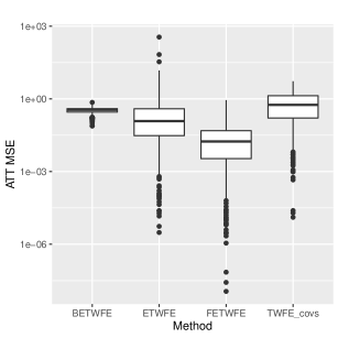
Figure 3: Boxplots of squared errors for each treatment effect estimate across all 700 simulations. Vertical axis is on a log scale.

Table 1: Means and standard errors for the squared error of the estimator of the ATT (25) for each method across all 700 simulations in the first simulation study from Section 7.

FETWFE	ETWFE	BETWFE	TWFE_COVS
0.0399 (0.00263)	1.19 (0.633)	0.339 (0.00336)	0.938 (0.0395)

Table 2: $p$-values from paired one-tailed $t$-tests of the alternative hypothesis that the FETWFE ATT estimator (35) has a lower squared estimation error for the ATT (25) than each competitor method calculated across all 700 simulations in the first simulation study from Section 7. (Low $p$-values indicate better predictive performance for FETWFE.)

ETWFE	BETWFE	TWFE_COVS
0.0343	1.24e-320	1.68e-86

In Appendix B, we also present estimation error results for the cohort-specific average treatment effects $\tau_{\text{ATT}}(r)$ as defined in (24) for each of the five cohorts, and estimation error for the coefficients of $\boldsymbol{\beta}_{N}^{*}$ corresponding to the interaction effects, $\boldsymbol{\rho}^{*}$. These results show that FETWFE outperforms the competitor methods for these estimands as well.

7.2 Restriction Selection Consistency

Next, we examine the extent to which we can trust FETWFE to select the correct restrictions, as we know it does with asymptotically high probability under Theorem 6.2. In the same experiment as before, on each simulation we calculate the percentage of restrictions FETWFE successfully identifies among the treatment parameters. In particular, we calculate the percentage of entries of $\boldsymbol{D}\boldsymbol{\beta}_{N}^{*}$ that FETWFE successfully estimates as either zero or nonzero.

On average across the 700 simulations, FETWFE successfully decides whether to use a restriction or not in $95.0\%$ of the $p_{N}$ possible cases, with a standard error of $0.025\%$. Of the true restrictions (that is, the entries of $\boldsymbol{D}\boldsymbol{\beta}_{N}^{*}$ that equal 0), on average $97.5\%$ ($0.021\%$) are correctly identified. This suggests that FETWFE is effective at identifying restrictions in practice, which contributes to FETWFE’s success in estimating treatment effects that we saw in the previous section. (Figure 4 in Appendix B shows a boxplot of the proportion of restrictions successfully identified across all 700 simulations.)

To get a better sense of the asymptotics, we conduct an additional simulation study in the same way as the first one, but with $T=5$, $R=3,d_{N}=2$ (resulting in $p_{N}=50$), and $N=1200$ observations (resulting in 300 observations per cohort in expectation). The sparse $\boldsymbol{\theta}_{N}^{*}$ is generated as before, but with entries each equalling 0 with probability 0.5. Again, we conduct 700 simulations. In this second simulation study, FETWFE successfully decides whether to use a restriction or not in $99.3\%$ ($0.042\%$) of the $p_{N}$ possible cases across the 700 simulations, and on average FETWFE identifies $98.5\%$ ($0.096\%$) of the true restrictions.

7.3 Asymptotic Distribution

Finally we investigate the asymptotic distribution of the FETWFE estimators. On each simulation, we estimate nominal $95\%$ confidence intervals for the cohort average treatment effects using the variance estimator from Theorem 6.4(a). In the first simulation study, we find coverage rates of 0.791 for the $r=2$ cohort (standard error 0.015), 0.884 for the $r=3$ cohort (standard error 0.012), $0.854$ (0.013) for the $r=4$ cohort, $0.803$ (0.015) for the $r=5$ cohort, and $0.850$ (0.014) for the $r=6$ cohort. We see that the coverage is unsatisfactory for FETWFE in this relatively small sample size, where in expectation 20 units are observed in each cohort.

We also estimate conservative confidence intervals for the average treatment effect with the conservative variance estimator from Theorem 6.4(c), yielding a coverage rate of 0.993 (0.001). That is, the conservative confidence intervals seem to satisfy the desired coverage level in practice, even though the asymptotic distribution of the test statistic is not known to be Gaussian (merely subgaussian).

Lastly, we examine the non-conservative estimator from Theorem 6.4(b): on each simulation study, we generate $N$ independent unlabeled samples where only cohort assignments (drawn from the same distribution as the $N$ labeled units) are observed, and we use these to estimate asymptotically exact confidence intervals for the average treatment effect. The resulting coverage is 0.986 (0.001). The coverage may be better for the average treatment effect than the cohort average treatment effects because the number of observations that are relevant for estimating the overall average treatment effect is much larger than that for each of the cohort average treatment effects.

In the second simulation study, described previously in Section 7.2, we find coverage rates of 0.944 (0.009) for the $r=2$ cohort, 0.941 (0.009) for the $r=3$ cohort, and 0.930 (0.010) for the third cohort. The conservative confidence intervals for the average treatment effects have coverage 0.997 (0.001), and the asymptotically exact confidence intervals have coverage 0.973 (0.002). Overall, the coverage rates are close to the nominal $95\%$ level in this finite $N$ setting.

8 Empirical Application

We analyze the data from Stevenson and Wolfers (2006), as collected in the divorce data set from Flack and Jee (2020). Stevenson and Wolfers estimate the causal effect of unilateral or “no-fault" divorce laws on suicide rates among women. The data set consists of observations from $N=51$ states (including the District of Columbia) for $T=33$ years, along with demographic covariates. The response variable is the aggregate state suicide rate among women by year (as in the first column of Table 1 of Stevenson and Wolfers 2006). See Stevenson and Wolfers (2006) and Goodman-Bacon (2021, Section III) for more details on the data.

We remove states treated at time $T=1$ from the data, leaving $N=42$ observations. 5 states are never treated, and $R=12$ cohorts are treated at various times. Similarly to the analysis in Goodman-Bacon (2021, Section IV(B)), we consider the time-varying covariates murderrate (state female homicide rate), lnpersinc (natural log of state personal income per capita), and afdcrolls (state welfare participation rate), including the values from time $t=1$ as time-invariant controls. However, murderrate is missing for some observations at $t=1$ and is omitted, leaving $d_{N}=2$ covariates. In total, we have $NT=1386$ observations and $p_{N}=908$ coefficients to estimate.

We estimate the variances $\sigma_{c}^{2}$ (the variance of the unit random effects) and $\sigma^{2}$ (the variance of the added noise) using the estimators from Pesaran (2015, Section 26.5.1) with ridge regression. We use FETWFE with $q=0.5$ to estimate the marginal average treatment effects, again leveraging the R grpreg package as in the simulation studies and selecting $\lambda_{N}$ by BIC. We estimate that the overall average percent change to the suicide rate for women is $-3.76\%$, which is similar to the estimate of $-2.52\%$ (standard error $1.09\%$) that Goodman-Bacon (2021) calculates when using similar controls. Applying Theorem 6.4(c), we estimate a conservative standard error of $4.70\%$, yielding a conservative $95\%$ confidence interval of $(-12.97\%,5.45\%)$ for the average treatment effect.

In Table 3 we present point estimates for the estimated average treatment effects for each of the cohorts. (We omit standard errors since the individual cohorts have very small sample sizes.) We estimate that four cohorts have non-zero treatment effects, with the 1970 cohort (consisting of California and Iowa) having by far the largest treatment effect estimate. We emphasize that these individual estimates are likely less reliable than the average treatment effect estimate since most cohorts have a small number of units.

Table 3: Cohort average treatment effect estimates from the empirical application in Section 8, targeting estimand $\tau_{\text{ATT}}(r)$ as defined in (24).

Cohort	$\hat{\tau}_{\text{ATT}}(r)$
1969	$0\%$
1970	-$40.142\%$
1971	$0\%$
1972	$0\%$
1973	-$3.466\%$
1974	$0\%$
1975	$0\%$
1976	-$4.703\%$
1977	-$5.338\%$
1980	$0\%$
1984	$0\%$
1985	$0\%$

9 Conclusion

In this work, we have proposed the fused extended two-way fixed effects estimator for difference-in-differences with staggered adoptions. Our estimator leverages the fact that the extended two-way fixed effects estimator includes coefficients that are likely to be similar (for example, because of their proximity in time), but it selects appropriate restrictions automatically rather than relying on hand-selected restrictions, which could be biased. FETWFE retains the asymptotic unbiasedness (and normality) of ETWFE but leverages sparsity for large efficiency gains. In particular, we showed that our estimator is consistent, selection consistent, asymptotically Gaussian, and oracle efficient for several classes of heterogeneous marginal and conditional average treatment effects. Finally, we demonstrated the usefulness of FETWFE in practice in both simulation studies and an empirical application.

9.1 Future Work

Throughout the paper we have mentioned places where our work might be relatively straightforward to extend. Here we specify some other possible extensions. It would be useful to develop theory allowing for FETWFE to be estimated when the design matrix $\boldsymbol{Z}$ is deficient in column rank; for example, when $p_{N}>NT$. One could extend our method to this setting by suitably adapting the marginal bridge estimator of Kock (2013), which involves a screening step to remove irrelevant covariates before estimating a regression on the reduced design matrix in a second step. This allows for consistency and asymptotic normality of the second-step estimator under similar assumptions to those that we have used in this work. Alternatively, consistency (but not asymptotic normality) could be established under weaker assumptions in the $q=1$ case by suitably adapting theory for lasso estimators like Corollary 2 from Negahban et al. (2012).

Another potentially useful extension would be relaxing the parallel trends assumption to allow for heterogeneous trends as described in Wooldridge (2021, Section 7.2). This requires adding extra parameters to the ETWFE estimator, but FETWFE is well-poised to adapt to this setting because it can automatically restrict to 0 any parameters that are added unnecessarily.

In Appendix A we investigate in more detail the relatively plausibility of conditional and marginal parallel trends, how Assumption (CIUU) interacts with these assumptions, and how we can achieve consistency of FETWFE for marginal average treatment effects under either form of parallel trends if (CIUU) holds. We present additional results from the simulation studies from Section 7 in Appendix B. We state Theorem C.1, which Theorems 6.1, 6.2, 6.3, and 6.4 all depend on, in Appendix C, and we prove it in Appendix E. We prove Theorems 6.1, 6.3, and 6.4 in Appendix D. In Appendix F we provide proofs for results that were stated but not proven in Appendix A and supporting results required to prove Theorems 6.1, 6.2, 6.3, and 6.4. We prove supporting results for Theorem C.1 in Appendix G. Finally, in Appendix H we explore the relationship between conditional and marginal parallel trends in more detail and state and prove some technical lemmas.

Appendix A More on Parallel Trends and Assumption (CIUU)

In Section A.1 we discuss the plausibility of marginal and conditional parallel trends in relation to an assumption of marginal or conditional (respectively) independence of the treatment and the potential outcomes. The latter assumptions imply the former, which motivates difference-in-differences estimators like FETWFE as more plausible than identification strategies that rely on stronger untestable assumptions.

We point out that no such strict hierarchy exists to relate marginal and conditional parallel trends in Section A.2—there exist settings where either assumption can hold without the other holding. Investigating this sheds light on when conditional or marginal parallel trends may be more plausible. We later show (Theorem A.5) that conditional parallel trends is necessary to estimate conditional average treatment effects via FETWFE, but there are estimators that are consistent for marginal average treatment effects under either conditional or marginal parallel trends. So it is natural to wonder whether an estimator could be consistent for marginal average treatment effects under either assumption. In Section A.3 we explore when this might hold, ultimately investigating Assumption (CIUU) in more detail and showing how it affects the consistency of regression (4). These ideas underlie the proof of Theorem 6.1.

A.1 Relationships Between Unconfounded Treatment Assignment, Marginally Randomized Treatment Assignment, and Parallel Trends Assumptions

In this section we present Proposition A.1, which relates the plausibility of several assumptions on the potential outcomes. Ultimately, this motivates difference-in-differences estimators like FETWFE as having more plausible untestable assumptions than methods that rely on unconfoundedness (like matching) or randomized assignment.

We consider an assumption of unconfoundedness of the untreated potential outcomes, which we define in this setting as

$$\tilde{y}_{it}(0)\mathchoice{\mathrel{\hbox to0.0pt{$\displaystyle\perp$\hss}\mkern 2.0mu{\displaystyle\perp}}}{\mathrel{\hbox to0.0pt{$\textstyle\perp$\hss}\mkern 2.0mu{\textstyle\perp}}}{\mathrel{\hbox to0.0pt{$\scriptstyle\perp$\hss}\mkern 2.0mu{\scriptstyle\perp}}}{\mathrel{\hbox to0.0pt{$\scriptscriptstyle\perp$\hss}\mkern 2.0mu{\scriptscriptstyle\perp}}}W_{i}\ \mid\ \boldsymbol{X}_{i}\qquad i\in[N],t\in\{1,\ldots,T\}.$$ (A.1)

This requires that treatment assignment is independent of the untreated potential outcomes conditional on the time-invariant (pre-treatment) covariates $\boldsymbol{X}_{i}$. Abadie [2005, Section 3.2.2] considered a similar assumption in the $T=2$ case. As we discuss in more detail later in this section, it has previously been noted that the assumption of unconfoundedness [Imbens and Rubin, 2015, Def. 3.6] that is common in causal inference is a stronger assumption than (CCTS).

Sometimes unconfoundedness is taken to be a stronger assumption that all of the potential outcomes are independent of treatment status conditional on covariates; such a condition would imply (A.1). Shaikh and Toulis [2021, Assumption 2.1] is one example of a work that uses such a stronger assumption in a setting with continuous treatment status.

We note that different notions of unconfoundedness have been considered in the difference-in-differences setting. For example, Imbens and Wooldridge [2009, Section 6.5.4] consider unconfoundedness in a two-period difference-in-differences setting with no covariates, where the lagged outcome is conditioned on rather than covariates. Similarly, Callaway and Li [2023] consider unconfoundedness conditional on several lagged time-varying variables. Ding and Li [2019] and Lindner and McConnell [2019] consider an ignorability condition where the untreated potential outcome is independent of treatment assignment status conditional on covariates and the lagged outcome.

We also refer to an assumption of marginal independence of the untreated potential outcomes and treatment status,

$$\tilde{y}_{it}(0)\mathchoice{\mathrel{\hbox to0.0pt{$\displaystyle\perp$\hss}\mkern 2.0mu{\displaystyle\perp}}}{\mathrel{\hbox to0.0pt{$\textstyle\perp$\hss}\mkern 2.0mu{\textstyle\perp}}}{\mathrel{\hbox to0.0pt{$\scriptstyle\perp$\hss}\mkern 2.0mu{\scriptstyle\perp}}}{\mathrel{\hbox to0.0pt{$\scriptscriptstyle\perp$\hss}\mkern 2.0mu{\scriptscriptstyle\perp}}}W_{i}\qquad i\in[N],t\in\{1,\ldots,T\}.$$ (A.2)

Completely randomized assignment, an assumption considered by, for example, Athey and Imbens [2022, Assumption 1] and Roth and Sant’Anna [2023, Case 1], is sufficient for (A.2).

Lastly, we say that (CCTS) or (CTS) holds in a transformation-invariant sense if (8) or (9) (respectively) hold under any transformation $g(\tilde{y}_{it}(r))$ of the potential outcomes such that the expectations exist. Some works have expressed concern that parallel trends assumptions are fragile because they may hold only if the response is not transformed, or only under a specific transformation [Meyer, 1995, Athey and Imbens, 2006, Kahn-Lang and Lang, 2020]. Roth and Sant’Anna [2023] investigate in detail when marginal parallel trends assumptions are transformation-invariant in the $T=2$ setting, and they point out that their arguments extend straightforwardly to the arbitrary $T$ setting as well as to conditional parallel trends assumptions. Proposition A.1 explicitly draws attention to an implication of their Propositions 3.1 and 3.2 when extended to these more general settings.

Proposition A.1.

Assume that the conditional expectations in (8) and (9) exist and are finite.

1. Unconfoundedness of the untreated potential outcomes is a strictly stronger assumption than conditional parallel trends: (A.1) is sufficient for Assumption CCTS to hold in a transformation-invariant sense, but (CCTS) does not imply unconfoundedness of the untreated potential outcomes.

2. Marginal independence of treatment status and the untreated potential outcomes is a strictly stronger assumption than marginal parallel trends: (A.2) is sufficient for Assumption CTS to hold in a transformation-invariant sense, but (CTS) does not imply (A.2).

Proof.

1. Under unconfoundedness (A.1), for any $i\in[N]$, $t\in\{1,\ldots,T\},r\in\mathcal{R}$ almost surely it holds that

   $$\mathbb{E}[h(\tilde{y}_{(it)}(0))\mid W_{i},\boldsymbol{X}_{i}]=\mathbb{E}[h(\tilde{y}_{(it)}(0))\mid\boldsymbol{X}_{i}]$$ (A.3)

   for any arbitrary $h(\cdot)$ such that the above expectation exists. For (CCTS) to hold with transformational invariance, we need that for any $h(\cdot)$ such that the expectations exist and any $i\in[N]$, $t\in\{2,\ldots,T\},r\in\mathcal{R}$, almost surely

   $$\mathbb{E}[h(\tilde{y}_{(it)}(0))-h(\tilde{y}_{(i1)}(0))\mid W_{i},\boldsymbol{X}_{i}]=\mathbb{E}[h(\tilde{y}_{(it)}(0))-h(\tilde{y}_{(i1)}(0))\mid\boldsymbol{X}_{i}].$$

   But this is immediate from (A.3). We show that the reverse implication does not hold by constructing a counterexample. (CCTS) can be rearranged as

   $$\mathbb{E}[\tilde{y}_{(it)}(0)\mid W_{i},\boldsymbol{X}_{i}]-\mathbb{E}[\tilde{y}_{(it)}(0)\mid\boldsymbol{X}_{i}]=\mathbb{E}[\tilde{y}_{(i1)}(0)\mid W_{i},\boldsymbol{X}_{i}]-\mathbb{E}[\tilde{y}_{(i1)}(0)\mid\boldsymbol{X}_{i}]\leavevmode\nobreak\ \forall t\in[T].$$ (A.4)

   Suppose that for all $t\in\{1,2,\ldots,T\}$, it holds that $\mathbb{E}[\tilde{y}_{(it)}(0)\mid W_{i},\boldsymbol{X}_{i}]-\mathbb{E}[\tilde{y}_{(it)}(0)\mid\boldsymbol{X}_{i}]=f(W_{i},\boldsymbol{X}_{i})$ almost surely for an arbitrary $f(\cdot,\cdot)$ that is not identically 0. Then from (A.4) we see that (CCTS) will hold. However, unconfoundedness does not hold since (A.3) with $h(\cdot)$ as the identity function is violated.

2. This proof is similar. Under marginal independence of treatment status and the untreated potential outcomes (A.2), for any $i\in[N]$, $t\in\{1,\ldots,T\},r\in\mathcal{R}$ almost surely it holds that

   $$\mathbb{E}[h(\tilde{y}_{(it)}(0))\mid W_{i}]=\mathbb{E}[h(\tilde{y}_{(it)}(0))]$$ (A.5)

   for any $h(\cdot)$ such that the expectation holds. It is immediate that for any such $h(\cdot)$ and any $i\in[N]$, $t\in\{2,\ldots,T\},r\in\mathcal{R}$, almost surely $\mathbb{E}[h(\tilde{y}_{(it)}(0))-h(\tilde{y}_{(i1)}(0))\mid W_{i}]=\mathbb{E}[h(\tilde{y}_{(it)}(0))-h(\tilde{y}_{(i1)}(0))]$, so (CTS) holds with transformational invariance. On the other hand, (CTS) can be rearranged as

   $$\mathbb{E}[\tilde{y}_{(it)}(0)\mid W_{i}]-\mathbb{E}[\tilde{y}_{(it)}(0)]=\mathbb{E}[\tilde{y}_{(i1)}(0)\mid W_{i}]-\mathbb{E}[\tilde{y}_{(i1)}(0)]\qquad\forall t\in[T].$$ (A.6)

   If for all $t\in\{1,2,\ldots,T\}$ we have $\mathbb{E}[\tilde{y}_{(it)}(0)\mid W_{i}]-\mathbb{E}[\tilde{y}_{(it)}(0)]=g(W_{i})$ almost surely for an arbitrary $g(\cdot)$ that is not identically 0, then (A.6) holds but (A.5) with $h(\cdot)$ as the identity function is violated. So (CTS) holds but marginal independence of treatment status and the untreated potential outcomes does not.

∎

Since unconfoundedness often seems more plausible than marginal independence of the potential outcomes and treatment status, Proposition A.1(a) and (b) considered together suggest an intuition that conditional parallel trends may often be more plausible than marginal parallel trends. Proposition A.1 also points out that difference-in-differences estimators are strictly more robust than identification strategies that rely on assumptions of completely randomized assignment or unconfoundedness.

Proposition A.1(a) verifies that (CCTS) is a strictly weaker assumption than unconfoundedness. As we mentioned earlier, this is a fairly straightforward observation that has been noted before; for example, Abadie [2005], Heckman et al. [1997], and Heckman et al. [1998] mention that this fact holds in the $T=2$ case. Besides the previously mentioned intuition that Proposition A.1(a) and (b) provide that conditional parallel trends may be more plausible in many applications than marginal parallel trends, we also draw attention to the facts in Proposition A.1(a) to point out explicitly that difference-in-differences identification strategies like FETWFE that rely on (CCTS) are more robust than methods like matching on time-invariant covariates that rely on an unconfoundedness assumption [Abadie and Imbens, 2006, Imbens and Rubin, 2015]. Proposition A.1(a) aligns with works like Chabé-Ferret [2015] which suggest that difference-in-differences with time-invariant covariates is more robust than matching. It is also consistent with the works like Chabé-Ferret [2017], Daw and Hatfield [2018], and Lindner and McConnell [2019], which show that combining matching on pre-treatment or time-invariant covariates with difference-in-differences estimation can fail to reduce bias, or even induce bias in treatment effect estimation in settings where difference-in-differences is unbiased.

The implications of Proposition A.1(b) are analogous, and previous works have also shown that random or “as good as random" treatment assignment is sufficient for (CTS) [Athey and Imbens, 2022, Roth and Sant’Anna, 2023, Ghanem et al., 2023].

A.2 Neither Conditional Nor Marginal Parallel Trends is Strictly More Plausible

Proposition A.1 showed that (CTS) and (CCTS) are strictly more plausible than (respectively) marginal independence of the potential outcomes and treatment and unconfoundedness. Theorem A.2 shows that (CTS) and (CCTS) cannot be related in this way—neither is strictly more plausible than the other.

Theorem A.2.

Assume that the conditional expectations in (8) and (9) exist and are finite. Neither of conditional parallel trends or marginal parallel trends is a relaxation of the other: Assumption CCTS (8) (conditional parallel trends) does not imply Assumption CTS (9) (marginal parallel trends), nor does (CTS) imply (CCTS).

Proof.

Provided in Appendix F.1.

∎

We prove Theorem A.2 by providing counterexamples where one of the parallel trends assumptions holds but the other does not. We briefly provide some intuition behind the counterexamples here in order to highlight some of the relative strengths and weaknesses of each assumption.

(CCTS) may hold when the time-invariant covariates have a time-varying effect on the potential outcomes, while (CTS) will not hold. This seems plausible if external conditions change that change the relevance of some features for the response. Ham and Miratrix [2022] and Callaway and Karami [2023] touch on closely related issues, investigating settings where parallel trends does not hold because time-invariant confounders have time-varying effects on the potential outcomes. We also expand on related ideas in Section A.3.

On the other hand, (CCTS) requires parallel trends to hold on every subgroup of $\boldsymbol{X}_{i}$. But (CTS) can hold if this is violated and parallel trends holds merely on average across the distribution of the covariates. That is, for any $r\in\{0\}\cup\mathcal{R}$, the quantity

$$\mathbb{E}[\tilde{y}_{(it)}(0)-\tilde{y}_{(i1)}(0)\mid W_{i}=r,\boldsymbol{X}_{i}]-\mathbb{E}[\tilde{y}_{(it)}(0)-\tilde{y}_{(i1)}(0)\mid\boldsymbol{X}_{i}]$$ (A.7)

may be positive on some subgroups of $\boldsymbol{X}_{i}$ if this is canceled out by (A.7) being negative on other subgroups such that (9) holds after marginalizing the left side of (8) across the distribution of $\boldsymbol{X}_{i}$ conditional on $W_{i}=r$ and the right side across the distribution of $\boldsymbol{X}_{i}$ conditional on $W_{i}=0$. In this particular sense, (CTS) allows for more variation in the time trends across the distribution of $\boldsymbol{X}_{i}$ than (CCTS). We also emphasize that both (CCTS) and (CTS) allow for heterogeneity in the sense that the values of $\mathbb{E}[\tilde{y}_{(it)}(0)-\tilde{y}_{(i1)}(0)\mid W_{i},\boldsymbol{X}_{i}]$ and $\mathbb{E}[\tilde{y}_{(it)}(0)-\tilde{y}_{(i1)}(0)\mid\boldsymbol{X}_{i}]$ may vary with $\boldsymbol{X}_{i}$.

However, if (8) does not hold, (9) holding exactly after marginalizing (8) appropriately may seem somewhat implausible. Nonetheless, it could be the case that (8) is not close to holding, but (9) approximately holds. Relaxing (CTS) by allowing small violations has been considered in recent works on sensitivity analyses for difference-in-differences estimation [Manski and Pepper, 2018, Ban and Kedagni, 2022, Rambachan and Roth, 2023, Ghanem et al., 2023]. That said, Ghanem et al. [2023, Section 7.2] point out that adjusting for covariates (that is, performing a sensitivity analysis under an assumption of conditional parallel trends that may not hold exactly) can result in smaller plausible ranges of marginal average treatment effects.

Overall, this suggests an intuition that (CCTS) may be somewhat more plausible in practice than (CTS), but since neither assumption nests the other, an ideal estimator would be asymptotically unbiased under either assumption. We discuss this in more detail in the next section.

A.3 Parallel Trends, Assumption (CIUU), and Regression (4)

Theorem A.2 motivates interest in estimators of marginal average treatment effects that are consistent under either conditional or marginal parallel trends. We have seen that Assumption (CIUU) is helpful for this—under the conditions of Theorem 6.1, FETWFE consistently estimates heterogeneous marginal average treatment effects under either conditional or marginal parallel trends if (CIUU) holds. In this section we fill in more detail about (CIUU), build some intuition for its role in the consistency of difference-in-differences estimators, and establish the consistency of regression (4) under (CIUU).

We first introduce a related assumption that, unlike (CIUU), is not directly testable.

Assumption (CIU) (“conditional independence of trends of the untreated potential outcomes"): Almost surely for all $r\in\{0\}\cup\mathcal{R}$, $i\in[N]$, and any $t\in\{2,\ldots,T\}$,

$$\mathbb{E}\left[\tilde{y}_{(it)}(0)-\tilde{y}_{(i1)}(0)\mid W_{i}=r\right]=\leavevmode\nobreak\ \mathbb{E}\left[\tilde{y}_{(it)}(0)-\tilde{y}_{(i1)}(0)\mid W_{i}=r,\boldsymbol{X}_{i}\right].$$

(CIU) is similar to (CIUU), but it requires the trends in the untreated potential outcomes to be mean-independent of $\boldsymbol{X}_{i}$ for units in all cohorts, so it cannot be tested.

It is immediate that (CCTS) and (CTS) are equivalent under (CIU).

Proposition A.3.

Under (CIU), conditional parallel trends (CCTS) and marginal parallel trends (CTS) are equivalent.

Proof.

We can apply (CIU) on each side of (CTS) to immediately yield that for any $i\in[N]$, $r\in\mathcal{R}$, and any $t\geq 2$,

$$\mathbb{E}[\tilde{y}_{(it)}(0)-\tilde{y}_{(i1)}(0)\mid W_{i}=r]=\leavevmode\nobreak\ \mathbb{E}[\tilde{y}_{(it)}(0)-\tilde{y}_{(i1)}(0)\mid W_{i}=0]$$

$$\iff\qquad\mathbb{E}[\tilde{y}_{(it)}(0)-\tilde{y}_{(i1)}(0)\mid W_{i}=r,\boldsymbol{X}_{i}]=\leavevmode\nobreak\ \mathbb{E}[\tilde{y}_{(it)}(0)-\tilde{y}_{(i1)}(0)\mid W_{i}=0,\boldsymbol{X}_{i}].$$

∎

One implication of Proposition A.3 is that any method that consistently estimates the marginal average treatment effects under either (CCTS) or (CTS) is parallel trends doubly-robust if (CIU) holds.

Although (CIUU) does not guarantee the equivalence of (CTS) and (CCTS), under (CIUU) conditional and marginal parallel trends are still connected.

Proposition A.4.

Suppose (CIUU) holds. Then conditional parallel trends (CCTS) implies marginal parallel trends (CTS).

Proof.

Applying (CIUU) to one side of (CCTS), we have that for any $i\in[N]$, $r\in\mathcal{R}$, and any $t\geq 2$,

$$\mathbb{E}[\tilde{y}_{(it)}(0)-\tilde{y}_{(i1)}(0)\mid W_{i}=r,\boldsymbol{X}_{i}]=\leavevmode\nobreak\ \mathbb{E}[\tilde{y}_{(it)}(0)-\tilde{y}_{(i1)}(0)\mid W_{i}=0,\boldsymbol{X}_{i}]$$

$$\iff\qquad\mathbb{E}[\tilde{y}_{(it)}(0)-\tilde{y}_{(i1)}(0)\mid W_{i}=r,\boldsymbol{X}_{i}]=\leavevmode\nobreak\ \mathbb{E}[\tilde{y}_{(it)}(0)-\tilde{y}_{(i1)}(0)\mid W_{i}=0]$$

$$\implies\leavevmode\nobreak\ \mathbb{E}\left[\mathbb{E}[\tilde{y}_{(it)}(0)-\tilde{y}_{(i1)}(0)\mid W_{i}=r,\boldsymbol{X}_{i}]\mid W_{i}=r\right]=\leavevmode\nobreak\ \mathbb{E}\left[\mathbb{E}[\tilde{y}_{(it)}(0)-\tilde{y}_{(i1)}(0)\mid W_{i}=0]\mid W_{i}=r\right]$$

$$\iff\qquad\mathbb{E}\left[\tilde{y}_{(it)}(0)-\tilde{y}_{(i1)}(0)\mid W_{i}=r\right]=\leavevmode\nobreak\ \mathbb{E}[\tilde{y}_{(it)}(0)-\tilde{y}_{(i1)}(0)\mid W_{i}=0].$$

∎

Proposition A.4 shows that any method that consistently estimates the marginal average treatment effects is also consistent under (CIUU) and (CCTS).

Notice that Assumptions (CIU) and (CIUU) are closely related to the time-varying effects of the covariates on the potential outcomes that we mentioned in our discussion of Theorem A.2 in Section A.2, which can cause marginal parallel trends to fail to hold even if conditional parallel trends holds. Proposition A.4 shows that (CIUU) rules out such settings.

Next we present a key result that underlies Theorem C.1, and in turn Theorems 6.1, 6.3, and 6.4.

Theorem A.5 (Assumption (CIUU) and the Consistency of Regression 4).

Assume that (CNAS) and (13) from (LINS) hold.

1. (Consistency under conditional parallel trends.) The following are equivalent: (i) conditional parallel trends after treatment (CCTSA) holds, and (ii) for all $r\in\mathcal{R}$ and all $t\geq r$, for the regression estimands $\tau_{rt}^{*}$ and $\boldsymbol{\rho}_{rt}^{*}$ defined in (13) it holds almost surely that the conditional average treatment effects $\tau_{\text{CATT}}(r,t,\boldsymbol{X}_{i})$ defined in (5) equal $\tau_{rt}^{*}+\left(\boldsymbol{X}_{i}-\mathbb{E}\left[\boldsymbol{X}_{i}\mid W_{i}=r\right]\right)^{\top}\boldsymbol{\rho}_{rt}^{*}$.

   (It follows from (ii) that each $\tau_{rt}^{*}$ is equal to the marginal average treatment effect $\tau_{\text{ATT}}(r,t)$ from Equation 1.)

2. (Consistency under marginal parallel trends and CIUU.) If (CIUU) and marginal parallel trends after treatment (CTSA) hold, then for all $r\in\mathcal{R}$ and all $t\geq r$ the regression estimand $\tau_{rt}^{*}$ is equal to the marginal average treatment effect $\tau_{\text{ATT}}(r,t)$.

3. (Identifying the bias-inducing covariates under CTSA if CIUU does not hold.) Suppose (CTSA) and (12) from (LINS) hold. Then for any $r\in\mathcal{R}$ and $t\in\{r,\ldots,T\}$,

   $$\tau_{rt}^{*}=\tau_{\text{ATT}}(r,t)-\left(\mathbb{E}[\boldsymbol{X}_{i}\mid W_{i}=r]-\mathbb{E}\left[\boldsymbol{X}_{i}\mid W_{i}=0\right]\right)^{\top}\boldsymbol{\xi}_{t}^{*}.$$

Proof.

The proofs of parts (b) and (c) are provided in Appendix F.1. Part (a) follows from Wooldridge [2021, Sections 6.3 and 6.4], but for illustrative purposes we provide a proof in our notation here. For all $r\in\mathcal{R},t\geq r$ and any $\boldsymbol{x}$ in the support of $\boldsymbol{X}_{i}$,

$$\tau_{rt}^{*}+\boldsymbol{\dot{x}}_{r}^{\top}\boldsymbol{\rho}_{rt}^{*}$$

$$\stackrel{{\scriptstyle(a)}}{{=}}\leavevmode\nobreak\ \mathbb{E}\left[\tilde{y}_{(it)}(r)-\tilde{y}_{(i1)}(r)\mid W_{i}=r,\boldsymbol{X}_{i}=\boldsymbol{x}\right]-\mathbb{E}\left[\tilde{y}_{(it)}(0)-\tilde{y}_{(i1)}(0)\mid W_{i}=0,\boldsymbol{X}_{i}=\boldsymbol{x}\right]$$

$$\stackrel{{\scriptstyle(b)}}{{=}}\leavevmode\nobreak\ \mathbb{E}[\tilde{y}_{(it)}(r)\mid W_{i}=r,\boldsymbol{X}_{i}=\boldsymbol{x}]-\bigg{(}\mathbb{E}[\tilde{y}_{(i1)}(0)\mid W_{i}=r,\boldsymbol{X}_{i}=\boldsymbol{x}]$$

$$+\mathbb{E}[\tilde{y}_{(it)}(0)-\tilde{y}_{(i1)}(0)\mid W_{i}=0,\boldsymbol{X}_{i}=\boldsymbol{x}]\bigg{)}$$

$$\stackrel{{\scriptstyle(c)}}{{=}}\leavevmode\nobreak\ \mathbb{E}[\tilde{y}_{(it)}(r)\mid W_{i}=r,\boldsymbol{X}_{i}=\boldsymbol{x}]-\mathbb{E}[\tilde{y}_{(it)}(0)\mid W_{i}=r,\boldsymbol{X}_{i}=\boldsymbol{x}]$$

$$=\leavevmode\nobreak\ \tau_{\text{CATT}}(r,t,\boldsymbol{x}),$$ (A.8)

where in $(a)$ we used (13) from (LINS), in $(b)$ we used (CNAS), and $(c)$ follows from rearranging (CCTSA).

∎

A.3.1 Discussion of Theorem A.5

Theorem A.5(a) and (b) show the consistency of regression (4): if (LINS), (CNAS), and (CIUU) hold, any estimator that is consistent for the regression estimands in (13) is also consistent for the marginal average treatment effects under either conditional parallel trends after treatment or marginal parallel trends after treatment. Theorem A.5(a) and (b) applies to ETWFE immediately under the conditions of Theorem 6.1(ii) in Wooldridge [2021], which shows that the ETWFE estimator of $\tau_{rt}^{*}$ is consistent. It also applies to FETWFE in light of Theorem C.1(b), which is used to prove Theorem 6.1.

Theorem A.5(c) shows that it is specifically the covariates $\boldsymbol{X}_{i}\mathbbm{1}\{t=t^{\prime}\}$ for $t^{\prime}\in\{2,\ldots,T\}$ (which correspond to regression estimands $\boldsymbol{\xi}_{t}^{*}$) included in regression (4) that induce an asymptotic bias in the estimated marginal average treatment effects $\tau_{\text{ATT}}(r,t^{\prime})$ if (CIUU) does not hold. Suppose we assume that (12) from (LINS) holds and $\boldsymbol{X}_{i}$ and $W_{i}$ are not mean-independent; in particular, for all $r\in\mathcal{R}$ we have $\mathbb{E}[\boldsymbol{X}_{i}\mid W_{i}=r]\neq\mathbb{E}[\boldsymbol{X}_{i}\mid W_{i}=0]$. Then if (CCTSA) and (CIUU) both do not hold, not only does Theorem A.5(a) show that there is no hope of estimating conditional average treatment effects, Theorem A.5(c) shows that in general including the covariates $\boldsymbol{X}_{i}\mathbbm{1}\{t=t^{\prime}\}$ in a regression induces bias in the estimated average treatment effects (since if (CIUU) does not hold and (12) from (LINS) does then $\boldsymbol{\xi}_{t}^{*}\neq\boldsymbol{0}$ for at least some $t$). This is true even if (CTS) holds and the marginal average treatment effects are estimable (by, for example, model (6.15) in Wooldridge 2021, which omits these covariates). That is, the covariates $\boldsymbol{X}_{i}\mathbbm{1}\{t=t^{\prime}\}$ for $t^{\prime}\in\{2,\ldots,T\}$ are “bad controls," in the language of Cinelli et al. [2022]. This observation aligns with the observation that Wooldridge [2021, Section 6.3] makes that including time-invariant covariates and their interactions with cohort dummies has no effect on the estimated marginal average treatment effects—it is specifically the inclusion of the covariate/time dummy interactions that changes the estimand for each $\tau_{rt}^{*}$.

Notice that these covariates correspond exactly to the kind of effect of the covariates on the untreated trends that is ruled out by Assumptions (CIU) and (CIUU), as well as the time-varying effects of the covariates on the potential outcomes that we mentioned in our discussion of Theorem A.2 in Section A.2.

However, if (12) holds, we see that under (CIUU) the coefficients $\boldsymbol{\xi}_{t}^{*}$ must all equal $\boldsymbol{0}$. In this case, Theorem A.5(c) shows that no harm is done to asymptotic unbiasedness by including those coefficients in the regression, and any estimator that is consistent for $\tau_{rt}^{*}$ from (13) is consistent for $\tau_{\text{ATT}}(r,t)$. (This aligns with part (b), which shows that if (CIUU) holds then we can consistently estimate the marginal average treatment effects under (CTSA) with regression 4.)

As we showed in Theorem 6.3, under the required assumptions no harm is done to the asymptotic efficiency of FETWFE by including irrelevant covariates (as we mentioned earlier in Remark 3.1), like when (CIUU) holds and all of the $\boldsymbol{\xi}_{t}^{*}$ equal $\boldsymbol{0}$.

Theorem A.5(c) has similarities to Theorems 4.1 and 5.1 from Ham and Miratrix [2022], which analyze the $T=2$, $\mathcal{R}=\{2\}$ and arbitrary $T$, $\mathcal{R}=\{T\}$ cases, respectively. In particular, their estimand $\mathbb{E}[\hat{\tau}_{\text{DiD}}^{X}]$ matches our estimand $\tau_{rt}^{*}$ under our assumptions, and they also identify the bias of this estimand in order to investigate when conditional parallel trends might be more plausible than marginal parallel trends. Besides the fact that we consider a more general staggered adoptions (arbitrary $\mathcal{R}$) setting, they also consider different structural equations for the potential outcomes (for example, they omit interactions between the covariates and treatment status or cohort membership, though they do allow for time-varying coefficients on the covariates) and they consider a setting with a latent confounder.

Appendix B Additional Results For Simulation Studies

Table 4 contains results for the cohort-specific squared estimation errors for the cohort-specific average treatment effects $\tau_{\text{ATT}}(r)$ as defined in (24). We see that on average FETWFE outperforms every method for most cohorts, except that BETWFE outperforms FETWFE for cohort 2. This is because the true treatment effect for Cohort 2 is close to 0 (0.069), so BETWFE’s direct penalization of the treatment coefficients directly towards 0 happens to be useful. Table 5 contains $p$-values for paired one-tailed $t$-tests of the alternative hypothesis that FETWFE has lower squared estimation error than the competitor methods, showing that the differences are statistically significant at the $0.01$ level in all settings except for the Cohort 2 BETWFE estimate and the last two ETWFE estimates, which are not significant because the ETWFE estimator has very high variance (see Table 4).

Table 6 contains results for the sum of squared errors of all methods’ estimates of the treatment interaction coefficients $\rho^{*}$. We see that FETWFE outperforms every method. Table 7 contains $p$-values for paired one-tailed $t$-tests of the alternative hypothesis that FETWFE has lower squared estimation error than the competitor methods, showing that the differences are statistically significant at the $0.05$ level.

Figure 4 depicts a boxplot of the proportion of the $p_{N}$ possible restrictions that FETWFE selects correctly in the first simulation study. Figures 5, 6, 7, 8, and 9 display boxplots of these squared errors, similar to Figure 3 for the average treatment effect. These plots also indicate that FETWFE typically outperforms the other methods.

Table 4: Means and standard errors for the squared errors of estimates of $\tau_{\text{ATT}}(r)$ by each method for each cohort in the simulation study from Section 7.

	FETWFE	ETWFE	BETWFE	TWFE_COVS
Cohort 2	0.035 (0.006)	1.502 (0.312)	0.008 (0)	7.265 (0.163)
Cohort 3	0.037 (0.004)	0.943 (0.19)	0.425 (0.011)	1.881 (0.091)
Cohort 4	0.129 (0.009)	0.856 (0.179)	3.492 (0.016)	1.269 (0.062)
Cohort 5	0.093 (0.007)	4.12 (3.079)	4.794 (0.011)	1.685 (0.082)
Cohort 6	0.068 (0.005)	3.212 (2.016)	3.759 (0.016)	0.949 (0.049)

Table 5: $p$-values for paired one-tailed $t$-tests of the alternative hypothesis that the FETWFE estimate of $\tau_{\text{ATT}}(r)$ has lower squared error than the competitor methods for each cohort in the simulation study from Section 7.

	ETWFE	BETWFE	TWFE_COVS
Cohort 2	1.14e-05	1	8.2e-206
Cohort 3	8.06e-06	2.35e-145	1.85e-72
Cohort 4	0.000119	0	3.89e-63
Cohort 5	0.118	0	1.12e-68
Cohort 6	0.0795	0	8.71e-60

Table 6: Means and standard errors for the summed squared errors of estimates of the treatment interaction coefficients $\boldsymbol{\rho}^{*}$ by each method for each cohort in the simulation study from Section 7.

fetwfe	etwfe	bridge_etwfe
0.529 (0.00827)	38.1 (18.3)	4.82 (0.0119)

Table 7: $p$-values for paired one-tailed $t$-tests of the alternative hypothesis that the FETWFE estimates of the treatment interaction coefficients $\boldsymbol{\rho}^{*}$ have lower summed squared error than the competitor methods for each cohort in the simulation study from Section 7.

etwfe	bridge_etwfe
0.02	0

Figure 4: Boxplot displaying proportions of correct treatment effect restriction decisions correctly made by FETWFE across each of the 700 simulations from the first simulation study in Section 7.

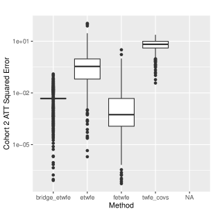
Figure 5: Boxplots of squared errors for each method’s estimate of $\tau_{\text{ATT}}(2)$ across all 700 simulations. Vertical axis is on a log scale.

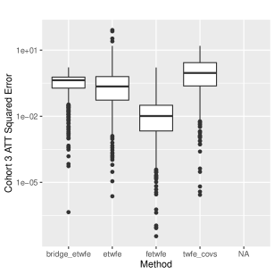
Figure 6: Boxplots of squared errors for each method’s estimate of $\tau_{\text{ATT}}(3)$ across all 700 simulations. Vertical axis is on a log scale.

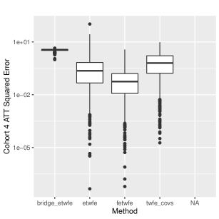
Figure 7: Boxplots of squared errors for each method’s estimate of $\tau_{\text{ATT}}(4)$ across all 700 simulations. Vertical axis is on a log scale.

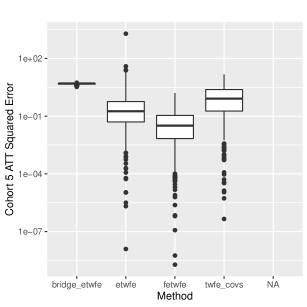
Figure 8: Boxplots of squared errors for each method’s estimate of $\tau_{\text{ATT}}(5)$ across all 700 simulations. Vertical axis is on a log scale.

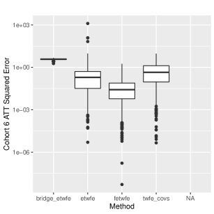
Figure 9: Boxplots of squared errors for each method’s estimate of $\tau_{\text{ATT}}(6)$ across all 700 simulations. Vertical axis is on a log scale.

Appendix C Theorem C.1

Theorem C.1 connects the bridge regression theory of Kock [2013] to the difference-in-differences theory of Wooldridge [2021]. It also makes use of some extensions of the theory of Kock [2013] (Theorem E.4, Theorem E.5). Equipped with Theorem C.1, Theorems 6.1, 6.2, and 6.4 are relatively straightforward to prove.

Theorem C.1.

1. (Correct specification.) Suppose Assumptions (CNAS), (CCTSB), and (LINS) hold. Then for all $i\in[N]$, $t\in[T]$, $r\in\mathcal{R}$,

   $$\mathbb{E}[\tilde{y}_{(it)}\mid W_{i}=0,\boldsymbol{X}_{i}]=\leavevmode\nobreak\ \eta^{*}+\gamma_{t}^{*}+\boldsymbol{X}_{i}^{\top}(\boldsymbol{\kappa}^{*}+\boldsymbol{\xi}_{t}^{*})\qquad\text{and}$$

   $$\mathbb{E}[\tilde{y}_{(it)}\mid W_{i}=r,\boldsymbol{X}_{i}]=\leavevmode\nobreak\ \eta^{*}+\gamma_{t}^{*}+\nu_{r}^{*}+\boldsymbol{X}_{i}^{\top}(\boldsymbol{\kappa}^{*}+\boldsymbol{\xi}_{t}^{*}+\boldsymbol{\zeta}_{r}^{*})+\mathbbm{1}\{t\geq r\}(\tau_{rt}^{*}+\boldsymbol{\dot{X}}_{(ir)}^{\top}\boldsymbol{\rho}_{rt}^{*}),$$

   where $\boldsymbol{\dot{X}}_{(ir)}=\boldsymbol{X}_{i}-\mathbb{E}[\boldsymbol{X}_{i}\mid W_{i}=r]$, for identifiability we define the time-dependent parameters to equal 0 at $t=1$, and recall that $\eta^{*},\gamma_{t}^{*}$, etc. are the regression estimands defined in (LINS).

2. (Estimation consistency.) In addition to the assumptions from part $(a)$, suppose Assumptions (F1), (F2), S($s_{N}$), and (R1) - (R3) hold. Then for any $q>0$, $\lVert\boldsymbol{\hat{\beta}}^{(q)}-\boldsymbol{\beta}_{N}^{*}\rVert_{2}=\mathcal{O}_{\mathbb{P}}\left(\min\{h_{N},h^{\prime}_{N}\}\right)$, where $h_{N}$ is defined in (38) and $h_{N}^{\prime}$ is defined in (37).

3. (Selection consistency.) Define

   $$\boldsymbol{\theta}_{N}^{*}:=\boldsymbol{D}_{N}\boldsymbol{\beta}_{N}^{*}$$ (C.1)

   and $\boldsymbol{\hat{\theta}}^{(q)}:=\boldsymbol{D}_{N}\boldsymbol{\hat{\beta}}^{(q)}$. In addition to the previous assumptions, assume that $q\in(0,1)$ and Assumptions (R4) - (R5) hold. Then $\lim_{N\to\infty}\mathbb{P}\left(\boldsymbol{\hat{\theta}}^{(q)}_{\mathcal{S}^{c}}=\boldsymbol{0}\right)=1$. (This also implies that $\boldsymbol{\hat{\theta}}^{(q)}_{\mathcal{S}^{c}}\xrightarrow{p}\boldsymbol{0}$, $\lim_{N\to\infty}\mathbb{P}\left(\sqrt{NT}\boldsymbol{\hat{\theta}}^{(q)}_{\mathcal{S}^{c}}=\boldsymbol{0}\right)=1$, and $\lim_{N\to\infty}\mathbb{P}\left(\sqrt{NT}\boldsymbol{v}_{N}^{\top}\boldsymbol{\hat{\theta}}^{(q)}_{\mathcal{S}^{c}}=0\right)=1$ for any sequence of finite vectors $\boldsymbol{v}_{N}\ \in\mathbb{R}^{p_{N}}$.)

   Further, let $\hat{\mathcal{S}}_{N}:=\{j:\hat{\theta}^{(q)}_{j}\neq 0\}$, and similarly let $\mathcal{S}_{N}\subseteq[p_{N}]$ be the set of components of $\boldsymbol{\theta}_{N}^{*}$ that are nonzero. Then

   $$\lim_{N\to\infty}\mathbb{P}\left(\hat{\mathcal{S}}_{N}=\mathcal{S}_{N}\right)=1.$$

4. (Asymptotic normality and oracle efficiency.) In addition to the previous assumptions, assume Assumption (R6) holds and Assumption S($s$) holds for a fixed $s_{N}=s$, so $\mathcal{S}_{N}=\mathcal{S}$ is fixed as well. Let $\{\boldsymbol{\psi}_{N}\}_{N=1}^{\infty}$ be a sequence of real-valued vectors where for each $\boldsymbol{\psi}_{N}\in\mathbb{R}^{p_{N}}$, $(\boldsymbol{\psi}_{N})_{\mathcal{S}}=\boldsymbol{\alpha}\in\mathbb{R}^{s}$ is fixed and finite and $(\boldsymbol{\psi}_{N})_{[p_{N}]\setminus\mathcal{S}}=\boldsymbol{b}_{N}$, where $\{\boldsymbol{b}_{N}\}_{N=1}^{\infty}$ is any sequence of constants where each $\boldsymbol{b}_{N}\in\mathbb{R}^{p_{N}-s}$ contains all finite entries. Then if $\boldsymbol{\alpha}\neq\boldsymbol{0}$,

   $$\sqrt{NT}\boldsymbol{\psi}_{N}^{\top}(\boldsymbol{\hat{\theta}}^{(q)}-\boldsymbol{\theta}_{N}^{*})\xrightarrow{d}\mathcal{N}\left(0,\sigma^{2}\boldsymbol{\alpha}^{\top}\left(\mathrm{Cov}\left(\boldsymbol{Z}\boldsymbol{D}_{N}^{-1}\right)_{(\cdot\cdot)\mathcal{S}}\right)^{-1}\boldsymbol{\alpha}\right),$$

   where $\mathrm{Cov}\left(\boldsymbol{Z}\boldsymbol{D}_{N}^{-1}\right)_{(\cdot\cdot)\mathcal{S}}$ is the columns and rows of the covariance matrix corresponding to the nonzero components of $\boldsymbol{\theta}_{N}^{*}$.

5. (Asymptotic normality with feasible variance estimator.) Maintain the assumptions from part $(d)$. For a random matrix $\boldsymbol{A}\in\mathbb{R}^{NT\times p_{N}}$, define

   $$\widehat{\mathrm{Cov}}(\boldsymbol{A}):=\frac{1}{NT}\left(\boldsymbol{A}-\mathbb{E}\boldsymbol{A}\right)^{\top}\left(\boldsymbol{A}-\mathbb{E}\boldsymbol{A}\right)$$ (C.2)

   to be the sample covariance matrix of $\boldsymbol{A}$. For any $\mathcal{A}_{N}\subseteq[p_{N}]$ such that $\mathcal{A}_{N}\neq\emptyset$, consider $\widehat{\mathrm{Cov}}\left((\boldsymbol{Z}\boldsymbol{D}_{N}^{-1})_{(\cdot\cdot)\mathcal{A}_{N}}\right)$, the estimated covariance matrix of the columns of $\boldsymbol{Z}\boldsymbol{D}_{N}^{-1}$ corresponding to $\mathcal{A}_{N}$. For sets $(\mathcal{A}_{N})_{N=1}^{\infty}$, define $\boldsymbol{\alpha}(\mathcal{A}_{N})\in\mathbb{R}^{|\mathcal{A}_{N}|}$ to be a fixed, finite vector for each unique $\mathcal{A}_{N}$, and define the sequence of $p_{N}$-vectors $\{\boldsymbol{\psi}_{N}(\mathcal{A}_{N})\}_{N=1}^{\infty}$ to have components in the entries corresponding to $\mathcal{A}_{N}$ equal to $\boldsymbol{\alpha}(\mathcal{A}_{N})$ and remaining entries $\boldsymbol{b}_{n}(\mathcal{A}_{N})$ all finite (but otherwise arbitrary). Define the sequence of random variables $U_{1}(\mathcal{A}_{N})$ to equal

   $$\frac{1}{\sigma}\sqrt{\frac{NT}{\boldsymbol{\alpha}(\mathcal{A}_{N})^{\top}\left(\widehat{\mathrm{Cov}}\left((\boldsymbol{Z}\boldsymbol{D}_{N}^{-1})_{(\cdot\cdot)\mathcal{A}_{N}}\right)\right)^{-1}\boldsymbol{\alpha}(\mathcal{A}_{N})}}\cdot\left(\boldsymbol{\psi}_{N}(\mathcal{A}_{N})^{\top}\boldsymbol{\hat{\theta}}^{(q)}-\boldsymbol{\psi}_{N}(\mathcal{S})^{\top}\boldsymbol{\theta}_{N}^{*}\right)$$

   if $\mathcal{A}_{N}\neq\emptyset$ and $\widehat{\mathrm{Cov}}\left((\boldsymbol{Z}\boldsymbol{D}_{N}^{-1})_{(\cdot\cdot)\mathcal{A}_{N}}\right)$ is invertible and 0 otherwise. Then if $\boldsymbol{\alpha}(\mathcal{S})\neq\boldsymbol{0}$,

   $$U_{1}(\hat{\mathcal{S}}_{N})\xrightarrow{d}\mathcal{N}(0,1).$$

6. (Asymptotic normality when $\boldsymbol{\alpha}$ is estimated independently from $\boldsymbol{\hat{\theta}}^{(q)}$.) Maintain the assumptions from part $(e)$. For sets $(\mathcal{A}_{N})_{N=1}^{\infty}$, let $\boldsymbol{\hat{\alpha}}_{N}(\mathcal{A}_{N})\in\mathbb{R}^{|\mathcal{A}_{N}|}$ be a sequence of random variables for each $\mathcal{A}_{N}$ with the properties that (1) for a given data set, $\mathcal{A}=\mathcal{A}^{\prime}$ implies $\boldsymbol{\hat{\alpha}}_{N}(\mathcal{A})=\boldsymbol{\hat{\alpha}}_{N}(\mathcal{A^{\prime}})$, (2) $\boldsymbol{\hat{\alpha}}_{N}(\mathcal{S})\xrightarrow{p}\boldsymbol{\alpha}$, and (3)

   $$\sqrt{NT}\left(\boldsymbol{\hat{\alpha}}_{N}(\mathcal{S})-\boldsymbol{\alpha}\right)\xrightarrow{d}\mathcal{N}(\boldsymbol{0}_{s},\boldsymbol{V}_{\psi}(\boldsymbol{\alpha}))$$

   for some positive semidefinite $\boldsymbol{V}_{\psi}(\boldsymbol{\alpha})\in\mathbb{R}^{s\times s}$. Define the sequence of random vectors $\{\boldsymbol{\hat{\psi}}_{N}(\mathcal{A}_{N})\}_{N=1}^{\infty}$ to have components in $\mathcal{A}_{N}$ equal to $\boldsymbol{\hat{\alpha}}(\mathcal{A}_{N})$ and components $\boldsymbol{\hat{b}}_{N}(\mathcal{A}_{N})$ in the components corresponding to $[p_{N}]\setminus\mathcal{A}_{N}$ that are all almost surely finite for all $N$. Define the sequence of random variables

   $$U_{2}(\mathcal{A}_{N}):=\sqrt{NT}\cdot\left(\boldsymbol{\hat{\psi}}_{N}(\mathcal{A}_{N})^{\top}\boldsymbol{\hat{\theta}}^{(q)}-\boldsymbol{\psi}_{N}(\mathcal{S})^{\top}\boldsymbol{\theta}_{N}^{*}\right).$$

   Assume $\boldsymbol{\hat{\alpha}}_{N}(\mathcal{A}_{N})$ and $\boldsymbol{\hat{\theta}}^{(q)}$ are estimated on independent data sets of size $N$. Then if $\boldsymbol{\alpha}\neq\boldsymbol{0}$,

   $$U_{2}(\hat{\mathcal{S}}_{N})\xrightarrow{d}\mathcal{N}\left(0,\sigma^{2}\boldsymbol{\alpha}^{\top}\left(\mathrm{Cov}\left((\boldsymbol{Z}\boldsymbol{D}_{N}^{-1})_{(\cdot\cdot)\mathcal{S}}\right)\right)^{-1}\boldsymbol{\alpha}+(\boldsymbol{\theta}_{N}^{*})^{\top}\boldsymbol{V}_{\psi}(\boldsymbol{\alpha})\boldsymbol{\theta}_{N}^{*}\right).$$

7. (Asymptotic normality when $\boldsymbol{\alpha}$ is estimated independently from $\boldsymbol{\hat{\theta}}^{(q)}$ with feasible variance estimator.) Maintain the assumptions from part $(f)$. Define the sequence of random variables $U_{3}(\mathcal{A}_{N})$ to equal

   $$\sqrt{\frac{NT}{\hat{v}_{N}(\mathcal{A}_{N})}}\cdot\left(\boldsymbol{\hat{\psi}}_{N}(\mathcal{A}_{N})^{\top}\boldsymbol{\hat{\theta}}^{(q)}-\boldsymbol{\psi}_{N}(\mathcal{S})^{\top}\boldsymbol{\theta}_{N}^{*}\right)$$

   if $\mathcal{A}_{N}\neq\emptyset$, $\boldsymbol{\hat{\alpha}}(\mathcal{A}_{N})\neq\boldsymbol{0}$, and $\widehat{\mathrm{Cov}}\left((\boldsymbol{Z}\boldsymbol{D}_{N}^{-1})_{(\cdot\cdot)\mathcal{A}_{N}}\right)$ is invertible and 0 otherwise, where

   $$\hat{v}_{N}(\mathcal{A}_{N}):=\sigma^{2}\boldsymbol{\hat{\alpha}}(\mathcal{A}_{N})^{\top}\left(\widehat{\mathrm{Cov}}\left((\boldsymbol{Z}\boldsymbol{D}_{N}^{-1})_{(\cdot\cdot)\mathcal{A}_{N}}\right)\right)^{-1}\boldsymbol{\hat{\alpha}}(\mathcal{A}_{N})+(\boldsymbol{\hat{\theta}}^{(q)})^{\top}\boldsymbol{\hat{V}}_{\psi}(\boldsymbol{\hat{\alpha}}_{N}(\mathcal{A}_{N}))\boldsymbol{\hat{\theta}}^{(q)}$$ (C.3)

   and $\boldsymbol{\hat{V}}_{\psi}(\boldsymbol{\hat{\alpha}}_{N}(\mathcal{A}_{N}))$ is an estimator of $\boldsymbol{V}_{\psi}(\boldsymbol{\alpha})$ that satisfies

   $$(\boldsymbol{\hat{\theta}}^{(q)}_{\mathcal{S}})^{\top}\boldsymbol{\hat{V}}_{\psi}(\boldsymbol{\hat{\alpha}}_{N}(\mathcal{S}))\boldsymbol{\hat{\theta}}^{(q)}_{\mathcal{S}}\xrightarrow{p}((\boldsymbol{\theta}^{*}_{N})_{\mathcal{S}})^{\top}\boldsymbol{V}_{\psi}(\boldsymbol{\alpha})(\boldsymbol{\theta}^{*}_{N})_{\mathcal{S}}.$$

   Assume $\boldsymbol{\hat{\alpha}}_{N}(\mathcal{A}_{N})$ and $\boldsymbol{\hat{\theta}}^{(q)}$ are estimated on independent data sets of size $N$. Then if $\boldsymbol{\alpha}\neq\boldsymbol{0}$,

   $$U_{3}(\hat{\mathcal{S}}_{N})\xrightarrow{d}\mathcal{N}(0,1).$$

8. (Asymptotic subgaussianity when $\boldsymbol{\alpha}$ is estimated on the same data set as $\boldsymbol{\hat{\theta}}^{(q)}$ with feasible variance estimator.) Maintain the assumptions from part $(g)$. Define the sequence of random variables $U_{4}(\mathcal{A}_{N})$ to equal

   $$\sqrt{\frac{NT}{\hat{v}_{N}^{(\text{cons})}(\mathcal{A}_{N})}}\cdot\left(\boldsymbol{\hat{\psi}}_{N}(\mathcal{A}_{N})^{\top}\boldsymbol{\hat{\theta}}^{(q)}-\boldsymbol{\psi}_{N}(\mathcal{S})^{\top}\boldsymbol{\theta}_{N}^{*}\right)$$

   if $\mathcal{A}_{N}\neq\emptyset$, $\boldsymbol{\hat{\alpha}}(\mathcal{A}_{N})\neq\boldsymbol{0}$, and $\widehat{\mathrm{Cov}}\left((\boldsymbol{Z}\boldsymbol{D}_{N}^{-1})_{(\cdot\cdot)\mathcal{A}_{N}}\right)$ is invertible and 0 otherwise, where $\hat{v}_{N}^{(\text{cons})}(\mathcal{A}_{N})$ is defined as

   $$\sigma^{2}\boldsymbol{\hat{\alpha}}(\mathcal{A}_{N})^{\top}\left(\widehat{\mathrm{Cov}}\left((\boldsymbol{Z}\boldsymbol{D}_{N}^{-1})_{(\cdot\cdot)\mathcal{A}_{N}}\right)\right)^{-1}\boldsymbol{\hat{\alpha}}(\mathcal{A}_{N})$$

   $$+2\sqrt{\sigma^{2}\boldsymbol{\hat{\alpha}}(\mathcal{A}_{N})^{\top}\left(\widehat{\mathrm{Cov}}\left((\boldsymbol{Z}\boldsymbol{D}_{N}^{-1})_{(\cdot\cdot)\mathcal{A}_{N}}\right)\right)^{-1}\boldsymbol{\hat{\alpha}}(\mathcal{A}_{N})(\boldsymbol{\hat{\theta}}^{(q)})^{\top}\boldsymbol{\hat{V}}_{\psi}(\boldsymbol{\hat{\alpha}}_{N}(\mathcal{A}_{N}))\boldsymbol{\hat{\theta}}^{(q)}}$$

   $$+(\boldsymbol{\hat{\theta}}^{(q)})^{\top}\boldsymbol{\hat{V}}_{\psi}(\boldsymbol{\hat{\alpha}}_{N}(\mathcal{A}_{N}))\boldsymbol{\hat{\theta}}^{(q)}$$ (C.4)

   and $\boldsymbol{\hat{V}}_{\psi}(\boldsymbol{\hat{\alpha}}_{N}(\mathcal{A}_{N}))$ is an estimator of $\boldsymbol{V}_{\psi}(\boldsymbol{\alpha})$ that satisfies

   $$(\boldsymbol{\hat{\theta}}^{(q)}_{\mathcal{S}})^{\top}\boldsymbol{\hat{V}}_{\psi}(\boldsymbol{\hat{\alpha}}_{N}(\mathcal{S}))\boldsymbol{\hat{\theta}}^{(q)}_{\mathcal{S}}\xrightarrow{p}((\boldsymbol{\theta}^{*}_{N})_{\mathcal{S}})^{\top}\boldsymbol{V}_{\psi}(\boldsymbol{\alpha})(\boldsymbol{\theta}^{*}_{N})_{\mathcal{S}}.$$

   Assume $\boldsymbol{\hat{\alpha}}_{N}(\mathcal{A}_{N})$ and $\boldsymbol{\hat{\theta}}^{(q)}$ are estimated on independent data sets of size $N$. Then if $\boldsymbol{\alpha}\neq\boldsymbol{0}$, $U_{4}(\hat{\mathcal{S}}_{N})$ converges in distribution to a mean-zero subgaussian random variable with variance at most 1.

Proof.

Provided in Section E. ∎

Appendix D Proofs of Main Results

D.1 Proofs of Theorems 6.1, 6.3, and 6.4

We present two lemmas we will use in the following proofs.

Lemma D.1.

The number of treatment effects $\mathfrak{W}$ is at most $(T-1)^{2}$. Further, after re-ordering the columns of $\boldsymbol{\tilde{Z}}$, we can write $\boldsymbol{D}_{N}$ as

$$\operatorname{diag}\big{(}\boldsymbol{D}^{(1)}(R),\boldsymbol{D}^{(1)}(T-1),\boldsymbol{I}_{d_{N}},\boldsymbol{I}_{d_{N}}\otimes\boldsymbol{D}^{(1)}(R),\boldsymbol{I}_{d_{N}}\otimes\boldsymbol{D}^{(1)}(T-1),\boldsymbol{D}^{(2)}(\mathcal{R}),\boldsymbol{I}_{d_{N}}\otimes\boldsymbol{D}^{(2)}(\mathcal{R})\big{)},$$ (D.1)

where $\boldsymbol{D}^{(1)}(t)\in\mathbb{R}^{t\times t}$ is defined in (F.4) and $\boldsymbol{D}^{(2)}(\mathcal{R})\in\mathbb{R}^{\mathfrak{W}\times\mathfrak{W}}$ is defined in (F.5). Further, $\boldsymbol{D}_{N}$ is invertible, and $\boldsymbol{D}_{N}^{-1}$ can be written as

$$\operatorname{diag}\Big{(} \boldsymbol{D}^{(1)}(R)^{-1},((\boldsymbol{D}^{(1)}(T-1))^{-1},\boldsymbol{I}_{d_{N}},\boldsymbol{I}_{d_{N}}\otimes\boldsymbol{D}^{(1)}(R)^{-1},\boldsymbol{I}_{d_{N}}\otimes((\boldsymbol{D}^{(1)}(T-1))^{-1},$$

$$(\boldsymbol{D}^{(2)}(\mathcal{R}))^{-1},\boldsymbol{I}_{d_{N}}\otimes(\boldsymbol{D}^{(2)}(\mathcal{R}))^{-1}\Big{)}.$$ (D.2)

Finally, both $\boldsymbol{D}_{N}$ and $\boldsymbol{D}_{N}^{-1}$ consists of blocks of size at most $(T-1)^{2}\times(T-1)^{2}$. For $\boldsymbol{D}_{N}$ the entries of these blocks are either $-1$, 0, or 1; and $\boldsymbol{D}_{N}^{-1}$ the entries of these blocks are either 0 or 1. Both matrices equal 0 elsewhere.

Lemma D.2.

Under Assumption (R3), $\max_{j\in p_{N}}\{|(\boldsymbol{\beta}_{N}^{*})_{j}|\}\leq(T-1)^{2}b_{1}$.

Proofs of both results are provided in Appendix F.2.

Proof of Theorem 6.1.

1. Observe that under our assumptions our model is correctly specified due to Theorem C.1(a). Recall that due to Theorem A.5,under our assumptions the regression estimands correspond to our causal estimands.

   Examining our estimator $\hat{\tau}_{\text{ATT}}(r,t)$ for the average treatment effect for a unit in cohort $r$ at time $t$ from (33), we see that we can then apply Theorem C.1(b) to immediately obtain that for every $r\in\mathcal{R}$ and $t\geq r$,

   $$\left|\hat{\tau}_{\text{ATT}}(r,t)-\tau_{\text{ATT}}(r,t)\right|=\left|\hat{\tau}_{rt}^{(q)}-\tau_{rt}^{*}\right|\leq\lVert\boldsymbol{\hat{\beta}}^{(q)}-\boldsymbol{\beta}_{N}^{*}\rVert_{2}=\mathcal{O}_{\mathbb{P}}\left(\min\{h_{N},h_{N}^{\prime}\}\right).$$ (D.3)

   Similarly, for any deterministic fixed linear combination of average treatment effects, using (D.3) and Theorem A.5 we have that for our class of estimators (34) and estimands (22),

   $$\left|\sum_{r\in\mathcal{R}}\sum_{t=r}^{T}\psi_{rt}\hat{\tau}_{\text{ATT}}(r,t)-\sum_{r\in\mathcal{R}}\sum_{t=r}^{T}\psi_{rt}\tau_{\text{ATT}}(r,t)\right|\leq\leavevmode\nobreak\ \sum_{r\in\mathcal{R}}\sum_{t=r}^{T}|\psi_{rt}|\left|\hat{\tau}_{\text{ATT}}(r,t)-\tau_{\text{ATT}}(r,t)\right|$$

   $$=\leavevmode\nobreak\ \mathcal{O}_{\mathbb{P}}\left(\min\{h_{N},h_{N}^{\prime}\}\right),$$

   where we used the fact that $T$ is fixed (and upper bounds $R$). Finally, for our class of estimators (35) and estimands (23), we have

   $$\left|\sum_{r\in\mathcal{R}}\sum_{t=r}^{T}\psi_{rt}\frac{N_{r}}{N_{\tau}}\hat{\tau}_{\text{ATT}}(r,t)-\psi_{rt}\tilde{\pi}_{r}\tau_{\text{ATT}}(r,t)\right|$$

   $$=\leavevmode\nobreak\ \left|\sum_{r\in\mathcal{R}}\sum_{t=r}^{T}\psi_{rt}\left(\frac{N_{r}}{N_{\tau}}\left(\hat{\tau}_{\text{ATT}}(r,t)-\tau_{\text{ATT}}(r,t)\right)-\left(\tilde{\pi}_{r}-\frac{N_{r}}{N_{\tau}}\right)\tau_{\text{ATT}}(r,t)\right)\right|$$

   $$\leq\leavevmode\nobreak\ \sum_{r\in\mathcal{R}}\sum_{t=r}^{T}|\psi_{rt}|\frac{N_{r}}{N_{\tau}}\left|\hat{\tau}_{\text{ATT}}(r,t)-\tau_{\text{ATT}}(r,t)\right|+\sum_{r\in\mathcal{R}}\sum_{t=r}^{T}\psi_{rt}\left|\tilde{\pi}_{r}-\frac{N_{r}}{N_{\tau}}\right|\left|\tau_{\text{ATT}}(r,t)\right|$$

   $$=\leavevmode\nobreak\ \mathcal{O}_{\mathbb{P}}(\min\{h_{N},h_{N}^{\prime}\})+\sum_{r\in\mathcal{R}}\left|\tilde{\pi}_{r}-\frac{N_{r}}{N_{\tau}}\right|\left|\frac{1}{T-r+1}\sum_{t=r}^{T}\tau_{rt}^{*}\right|,$$

   where we used that $N_{r}/N_{\tau}\in[0,1]$ for all $r$ and (D.3). (Recall that $N_{r}=\sum_{i=1}^{N}\mathbbm{1}\{W_{i}=r\}$ the total number of units in cohort $r$ and $N_{\tau}=N^{-1}\sum_{i=1}^{N}\mathbbm{1}\{W_{i}\neq 0\}=\sum_{r^{\prime}\in\mathcal{R}}N_{r^{\prime}}$ is the total number of treated units.) We will show that the second term in this sum is $\mathcal{O}_{\mathbb{P}}(1/\sqrt{N})$. By Theorem 14.6 in Wasserman [2004],

   $$\sqrt{N}\left(\frac{N_{0}}{N}-\pi_{0},\frac{N_{r_{1}}}{N}-\pi_{r_{1}},\ldots,\frac{N_{r_{R}}}{N}-\pi_{r_{R}}\right)\xrightarrow{d}\mathcal{N}\left(\boldsymbol{0},\boldsymbol{\Sigma}_{M}\right),$$

   where

   $$\boldsymbol{\Sigma}_{M}:=\begin{pmatrix}\pi_{0}(1-\pi_{0})&-\pi_{0}\pi_{r_{1}}&\cdots&-\pi_{0}\pi_{r_{R}}\\ -\pi_{0}\pi_{r_{1}}&\pi_{r_{1}}(1-\pi_{r_{1}})&\cdots&-\pi_{r_{1}}\pi_{r_{R}}\\ \vdots&\vdots&\ddots&\vdots\\ -\pi_{0}\pi_{r_{R}}&-\pi_{r_{1}}\pi_{r_{R}}&\cdots&\pi_{r_{R}}(1-\pi_{r_{R}})\end{pmatrix}\in\mathbb{R}^{(R+1)\times(R+1)}.$$ (D.4)

   Therefore

   $$\left\lVert\sqrt{N}\left(\frac{N_{0}}{N}-\pi_{0},\frac{N_{r_{1}}}{N}-\pi_{r_{1}},\ldots,\frac{N_{r_{R}}}{N}-\pi_{r_{R}}\right)-\mathcal{N}\left(\boldsymbol{0},\boldsymbol{\Sigma}_{M}\right)\right\rVert_{2}=o_{\mathbb{P}}(1),$$

   so

   $$\sqrt{N}\left\lVert\left(\frac{N_{0}}{N}-\pi_{0},\frac{N_{r_{1}}}{N}-\pi_{r_{1}},\ldots,\frac{N_{r_{R}}}{N}-\pi_{r_{R}}\right)\right\rVert_{2}\leq\lVert\mathcal{N}\left(\boldsymbol{0},\boldsymbol{\Sigma}_{M}\right)\rVert_{2}+o_{\mathbb{P}}(1)=\mathcal{O}_{\mathbb{P}}(1),$$

   so

   $$\left\lVert\left(\frac{N_{0}}{N}-\pi_{0},\frac{N_{r_{1}}}{N}-\pi_{r_{1}},\ldots,\frac{N_{r_{R}}}{N}-\pi_{r_{R}}\right)\right\rVert_{2}=\mathcal{O}_{\mathbb{P}}\left(\frac{1}{\sqrt{N}}\right)$$

   and for all $r\in\mathcal{R}$

   $$\left|\tilde{\pi}_{r}-\frac{N_{r}}{N_{\tau}}\right|\leq\left\lVert\left(\frac{N_{0}}{N}-\pi_{0},\frac{N_{r_{1}}}{N}-\pi_{r_{1}},\ldots,\frac{N_{r_{R}}}{N}-\pi_{r_{R}}\right)\right\rVert_{2}=\mathcal{O}_{\mathbb{P}}\left(\frac{1}{\sqrt{N}}\right).$$

   Since

   $$\left|\frac{1}{T-r+1}\sum_{t=r}^{T}\tau_{rt}^{*}\right|$$

   is finite under our assumptions due to Lemma D.2 (and the fact that $T$ is finite), we have

   $$\left|\sum_{r\in\mathcal{R}}\sum_{t=r}^{T}\psi_{rt}\frac{N_{r}}{N_{\tau}}\hat{\tau}_{\text{ATT}}(r,t)-\psi_{rt}\tilde{\pi}_{r}\tau_{\text{ATT}}(r,t)\right|=\leavevmode\nobreak\ \mathcal{O}_{\mathbb{P}}(\min\{h_{N},h_{N}^{\prime}\})+\mathcal{O}_{\mathbb{P}}(1/\sqrt{N})$$

   $$=\leavevmode\nobreak\ \mathcal{O}_{\mathbb{P}}(\min\{h_{N},h_{N}^{\prime}\}),$$

   where in the last step we used that $1/\sqrt{N}=\mathcal{O}(h_{N})$ since $e_{1N}$ is upper-bounded by a constant and $p_{N}$ is nondecreasing.

2. Again, using Theorem A.5,

   $$\tau_{\text{CATT}}(\boldsymbol{x},r,t)=\tau_{rt}^{*}+(\boldsymbol{\rho}_{rt}^{*})^{\top}\left(\boldsymbol{x}-\mathbb{E}\left[\boldsymbol{X}_{(1t)\cdot}\mid W_{i}=r\right]\right)=\tau_{rt}^{*}+(\boldsymbol{\rho}_{rt}^{*})^{\top}\left(\boldsymbol{x}-\boldsymbol{\mu}_{r}\right),$$

   where $\boldsymbol{\mu}_{r}:=\mathbb{E}\left[\boldsymbol{X}_{(it)\cdot}\mid W_{i}=r\right]$. Using this and (30) we have

   $$\left|\hat{\tau}_{\text{CATT}}(r,t,\boldsymbol{x})-\tau_{\text{CATT}}(r,t,\boldsymbol{x})\right|$$

   $$=\leavevmode\nobreak\ \left|\hat{\tau}_{rt}^{(q)}-\tau_{rt}^{*}+(\boldsymbol{x}-\boldsymbol{\overline{X}}_{r})^{\top}\boldsymbol{\hat{\rho}}_{rt}-\left(\boldsymbol{x}-\boldsymbol{\mu}_{r}\right)^{\top}\boldsymbol{\rho}_{rt}^{*}\right|$$

   $$=\leavevmode\nobreak\ \left|\hat{\tau}_{rt}^{(q)}-\tau_{rt}^{*}+\left(\boldsymbol{x}-\boldsymbol{\mu}_{r}\right)^{\top}\left(\boldsymbol{\hat{\rho}}_{rt}-\boldsymbol{\rho}_{rt}^{*}\right)+\left(\boldsymbol{\mu}_{r}-\boldsymbol{\overline{X}}_{r}\right)^{\top}\left(\boldsymbol{\hat{\rho}}_{rt}-\boldsymbol{\rho}_{rt}^{*}\right)-\left(\boldsymbol{\overline{X}}_{r}-\boldsymbol{\mu}_{r}\right)^{\top}\boldsymbol{\rho}_{rt}^{*}\right|$$

   $$\leq\leavevmode\nobreak\ \left|\hat{\tau}_{rt}^{(q)}-\tau_{rt}^{*}\right|+\left|\left(\boldsymbol{x}-\boldsymbol{\mu}_{r}\right)^{\top}\left(\boldsymbol{\hat{\rho}}_{rt}-\boldsymbol{\rho}_{rt}^{*}\right)\right|+\left|\left(\boldsymbol{\mu}_{r}-\boldsymbol{\overline{X}}_{r}\right)^{\top}\left(\boldsymbol{\hat{\rho}}_{rt}-\boldsymbol{\rho}_{rt}^{*}\right)\right|+\left|\left(\boldsymbol{\overline{X}}_{r}-\boldsymbol{\mu}_{r}\right)^{\top}\boldsymbol{\rho}_{rt}^{*}\right|$$

   $$\stackrel{{\scriptstyle(a)}}{{\leq}}\leavevmode\nobreak\ \left|\hat{\tau}_{rt}^{(q)}-\tau_{rt}^{*}\right|+\left\lVert\boldsymbol{x}-\boldsymbol{\mu}_{r}\right\rVert_{2}\left\lVert\boldsymbol{\hat{\rho}}_{rt}-\boldsymbol{\rho}_{rt}^{*}\right\rVert_{2}+\left\lVert\boldsymbol{\mu}_{r}-\boldsymbol{\overline{X}}_{r}\right\rVert_{2}\left\lVert\boldsymbol{\hat{\rho}}_{rt}-\boldsymbol{\rho}_{rt}^{*}\right\rVert_{2}+\left\lVert\boldsymbol{\overline{X}}_{r}-\boldsymbol{\mu}_{r}\right\rVert_{2}\left\lVert\boldsymbol{\rho}_{rt}^{*}\right\rVert_{2}$$

   $$\stackrel{{\scriptstyle(b)}}{{=}}\leavevmode\nobreak\ \mathcal{O}_{\mathbb{P}}(\min\{h_{N},h_{N}^{\prime}\})+\mathcal{O}_{\mathbb{P}}(\min\{h_{N},h_{N}^{\prime}\})+\mathcal{O}_{\mathbb{P}}\left(1/\sqrt{N}\right)\mathcal{O}_{\mathbb{P}}\left(\min\{h_{N},h_{N}^{\prime}\}\right)+\mathcal{O}_{\mathbb{P}}\left(1/\sqrt{N}\right)$$

   $$=\leavevmode\nobreak\ \mathcal{O}_{\mathbb{P}}(\min\{h_{N},h_{N}^{\prime}\}),$$

   where in $(a)$ we applied Cauchy-Schwarz and $(b)$ follows from Theorem C.1, the fact that $\left\lVert\boldsymbol{\rho}_{rt}^{*}\right\rVert_{2}$ is fixed and bounded since $d$ is fixed and each coefficient is finite due to Lemma D.2, and Lemma D.3:

   Lemma D.3.

   Suppose $d_{N}=d$ is fixed. Then under Assumption (R1),

   $$\left\lVert\boldsymbol{\overline{X}}_{r}-\boldsymbol{\mu}_{r}\right\rVert_{2}=\leavevmode\nobreak\ \mathcal{O}_{\mathbb{P}}\left(\frac{1}{\sqrt{N}}\right).$$

   Proof.

   Provided in Appendix F.2. ∎

   Next, for any deterministic fixed set of constants $\{\psi_{rt}\}$, the above result gives us

   $$\left|\sum_{r\in\mathcal{R}}\sum_{t=r}^{T}\psi_{rt}\hat{\tau}_{\text{CATT}}(r,t,\boldsymbol{x})-\sum_{r\in\mathcal{R}}\sum_{t=r}^{T}\psi_{rt}\tau_{\text{CATT}}(r,t,\boldsymbol{x})\right|$$

   $$\leq\leavevmode\nobreak\ \sum_{r\in\mathcal{R}}\sum_{t=r}^{T}|\psi_{rt}|\left|\hat{\tau}_{\text{CATT}}(r,t,\boldsymbol{x})-\tau_{\text{CATT}}(r,t,\boldsymbol{x})\right|$$

   $$=\leavevmode\nobreak\ \mathcal{O}_{\mathbb{P}}(\min\{h_{N},h_{N}^{\prime}\}).$$ (D.5)

   Finally, for any deterministic fixed set of constants $\{\psi_{rt}\}$ we have

   $$\left|\sum_{r\in\mathcal{R}}\sum_{t=r}^{T}\psi_{rt}\left(\frac{\hat{\pi}_{r}(\boldsymbol{x})}{\sum_{r^{\prime}\in\mathcal{R}}\hat{\pi}_{r^{\prime}}(\boldsymbol{x})}\right)\hat{\tau}_{\text{CATT}}(r,t,\boldsymbol{x})-\sum_{r\in\mathcal{R}}\sum_{t=r}^{T}\psi_{rt}\tilde{\pi}_{r}(\boldsymbol{x})\tau_{\text{CATT}}(r,t,\boldsymbol{x})\right|$$

   $$=\leavevmode\nobreak\ \Bigg{|}\sum_{r\in\mathcal{R}}\sum_{t=r}^{T}\psi_{rt}\left(\frac{\hat{\pi}_{r}(\boldsymbol{x})}{\sum_{r^{\prime}\in\mathcal{R}}\hat{\pi}_{r^{\prime}}(\boldsymbol{x})}\right)(\hat{\tau}_{\text{CATT}}(r,\boldsymbol{x},t)-\tau_{\text{CATT}}(r,t,\boldsymbol{x}))$$

   $$-\sum_{r\in\mathcal{R}}\sum_{t=r}^{T}\psi_{rt}\left[\tilde{\pi}_{r}(\boldsymbol{x})-\frac{\hat{\pi}_{r}(\boldsymbol{x})}{\sum_{r^{\prime}\in\mathcal{R}}\hat{\pi}_{r^{\prime}}(\boldsymbol{x})}\right]\tau_{\text{CATT}}(r,t,\boldsymbol{x})\Bigg{|}$$

   $$\leq\leavevmode\nobreak\ \sum_{r\in\mathcal{R}}\sum_{t=r}^{T}|\psi_{rt}|\left|\frac{\hat{\pi}_{r}(\boldsymbol{x})}{\sum_{r^{\prime}\in\mathcal{R}}\hat{\pi}_{r^{\prime}}(\boldsymbol{x})}\right|\left|\hat{\tau}_{\text{CATT}}(r,\boldsymbol{x},t)-\tau_{\text{CATT}}(r,t,\boldsymbol{x})\right|$$

   $$+\sum_{r\in\mathcal{R}}\sum_{t=r}^{T}|\psi_{rt}|\left|\tilde{\pi}_{r}(\boldsymbol{x})-\frac{\hat{\pi}_{r}(\boldsymbol{x})}{\sum_{r^{\prime}\in\mathcal{R}}\hat{\pi}_{r^{\prime}}(\boldsymbol{x})}\right|\left|\tau_{\text{CATT}}(r,t,\boldsymbol{x})\right|$$

   $$\leq\leavevmode\nobreak\ \sum_{r\in\mathcal{R}}\sum_{t=r}^{T}|\psi_{rt}|\left|\hat{\tau}_{\text{CATT}}(r,t,\boldsymbol{x})-\tau_{\text{CATT}}(r,t,\boldsymbol{x})\right|$$

   $$+\sum_{r\in\mathcal{R}}\sum_{t=r}^{T}|\psi_{rt}|\left|\tilde{\pi}_{r}(\boldsymbol{x})-\frac{\hat{\pi}_{r}(\boldsymbol{x})}{\sum_{r^{\prime}\in\mathcal{R}}\hat{\pi}_{r^{\prime}}(\boldsymbol{x})}\right|\left|\tau_{\text{CATT}}(r,t,\boldsymbol{x})\right|$$

   $$=\leavevmode\nobreak\ \mathcal{O}_{\mathbb{P}}(\min\{h_{N},h_{N}^{\prime}\})+\sum_{r\in\mathcal{R}}\sum_{t=r}^{T}|\psi_{rt}|\left|\tilde{\pi}_{r}(\boldsymbol{x})-\frac{\hat{\pi}_{r}(\boldsymbol{x})}{\sum_{r^{\prime}\in\mathcal{R}}\hat{\pi}_{r^{\prime}}(\boldsymbol{x})}\right|\left|\tau_{\text{CATT}}(r,t,\boldsymbol{x})\right|,$$

   where we used (D.5) and the fact that $|\psi_{rt}|$ is bounded for any fixed $\boldsymbol{x}$ for all $r\in\mathcal{R}$ due to Lemma D.2. The second part of the result then follows from our assumption that

   $$\left|\tilde{\pi}_{r}(\boldsymbol{x})-\frac{\hat{\pi}_{r}(\boldsymbol{x})}{\sum_{r^{\prime}\in\mathcal{R}}\hat{\pi}_{r^{\prime}}(\boldsymbol{x})}\right|=\mathcal{O}_{\mathbb{P}}(a_{N})$$

   and the fact that $|\psi_{rt}|\left|\tau_{\text{CATT}}(r,t,\boldsymbol{x})\right|$ is bounded for any fixed $\boldsymbol{x}$. The first part follows from this argument: since $\hat{\pi}_{r}(\boldsymbol{x})\xrightarrow{p}\pi_{r}(\boldsymbol{x})$ for any fixed $\boldsymbol{x}$ for all $r\in\{0\}\cup\mathcal{R}$ and $\pi_{r}(\boldsymbol{x})>0$ for all $r\in\{0\}\cup\mathcal{R}$ by Assumption (F2), the continuous mapping theorem implies

   $$\frac{\hat{\pi}_{r}(\boldsymbol{x})}{\sum_{r^{\prime}\in\mathcal{R}}\hat{\pi}_{r^{\prime}}(\boldsymbol{x})}\xrightarrow{p}\frac{\pi_{r}(\boldsymbol{x})}{\sum_{r^{\prime}\in\mathcal{R}}\pi_{r^{\prime}}(\boldsymbol{x})}=\tilde{\pi}_{r}(\boldsymbol{x})$$

   for all $r\in\mathcal{R}$. It follows that

   $$\sum_{r\in\mathcal{R}}\left|\tilde{\pi}_{r}(\boldsymbol{x})-\frac{\hat{\pi}_{r}(\boldsymbol{x})}{\sum_{r^{\prime}\in\mathcal{R}}\hat{\pi}_{r^{\prime}}(\boldsymbol{x})}\right|\left|\tau_{\text{CATT}}(r,\boldsymbol{x})\right|\xrightarrow{p}0.$$

   In combination with (D.5) and Slutsky’s theorem, this proves the result.

∎

We prove Theorem 6.4 before proving Theorem 6.3.

Proof of Theorem 6.4.

By Theorem A.5, the average treatment effect $\tau_{\text{ATT}}(r,t)$ is equal to the regression estimand $\tau_{rt}^{*}$. We will prove Theorem 6.4 by applying Theorem C.1(e), (g), and (h) with particular choices of vectors $\boldsymbol{\psi}_{N}$ and $\boldsymbol{\hat{\psi}}_{N}$.

1. Let $i(r,t)$ be the index of the row of $\boldsymbol{D}_{N}$ corresponding to $\hat{\tau}_{rt}^{(q)}$ (that is, the column of $\boldsymbol{\tilde{Z}}$ corresponding to this regression coefficient), so that

   $$\hat{\tau}_{rt}^{(q)}=(\boldsymbol{D}_{N}^{-1})_{i(r,t)\cdot}\boldsymbol{\hat{\theta}}^{(q)}$$

   and

   $$\tau_{rt}^{*}=(\boldsymbol{D}_{N}^{-1})_{i(r,t)\cdot}\boldsymbol{\theta}_{N}^{*}.$$

   Since we can see from Lemma D.1 that each row of $\boldsymbol{D}_{N}^{-1}$ contains at most $(T-1)^{2}$ nonzero entries, all of the nonzero entries equal 1, and the entries corresponding to the $s$ relevant features will stay fixed even if $p_{N}\to\infty$, the vector $\boldsymbol{\psi}_{N}=\left((\boldsymbol{D}_{N}^{-1})_{i(r,t),\cdot}\right)^{\top}$ is a valid choice for Theorem C.1(d), (e), and (f). In fact, any fixed, finite linear combination of rows $(\boldsymbol{D}_{N}^{-1})_{i(r,t),\cdot}$ is a valid choice. We therefore have from Theorem C.1(e) that if at least one of the nonzero components of $(\boldsymbol{D}_{N}^{-1})_{i(r,t),\cdot}$ corresponds to one of the $s$ features in $\mathcal{S}$,

   $$\sqrt{\frac{NT}{\hat{v}_{N}^{\text{ATT};r,t}}}\left((\boldsymbol{D}_{N}^{-1})_{i(r,t),\cdot}\boldsymbol{\hat{\theta}}^{(q)}-(\boldsymbol{D}_{N}^{-1})_{i(r,t),\cdot}\boldsymbol{\theta}_{N}^{*}\right)\xrightarrow{d}\leavevmode\nobreak\ \mathcal{N}(0,1)$$

   $$\iff\qquad\sqrt{\frac{NT}{\hat{v}_{N}^{\text{ATT};r,t}}}\left(\hat{\tau}_{\text{ATT}}(r,t)-\tau_{\text{ATT}}(r,t)\right)\xrightarrow{d}\leavevmode\nobreak\ \mathcal{N}(0,1),$$

   where

   $$\hat{v}_{N}^{\text{ATT};r,t}:=\sigma^{2}(\boldsymbol{D}_{N}^{-1})_{i(r,t),\hat{\mathcal{S}}}\left(\widehat{\mathrm{Cov}}\left((\boldsymbol{Z}[\boldsymbol{D}_{N}^{-1}]^{\top})_{(\cdot\cdot)\hat{\mathcal{S}}}\right)\right)^{-1}((\boldsymbol{D}_{N}^{-1})_{i(r,t),\hat{\mathcal{S}}})^{\top},$$

   $\widehat{\mathrm{Cov}}(\cdot)$ is defined in (C.2) and $(\boldsymbol{D}_{N}^{-1})_{i(r,t),\hat{\mathcal{S}}}\in\mathbb{R}^{|\hat{\mathcal{S}}|}$ is a row vector that contains the $|\hat{\mathcal{S}}|$ components of the $i(r,t)$ row of $\boldsymbol{D}_{N}^{-1}$ corresponding to the selected features. Similarly, for any deterministic fixed set of constants $\{\psi_{rt}\}$, since

   $$\sum_{r\in\mathcal{R}}\sum_{t=r}^{T}\psi_{rt}\tau_{rt}^{*}=\sum_{r\in\mathcal{R}}\sum_{t=r}^{T}\psi_{rt}(\boldsymbol{D}_{N}^{-1})_{i(r,t),\cdot}\boldsymbol{\theta}_{N}^{*},$$

   we can choose $\boldsymbol{\psi}_{N}^{(\text{C})}:=\sum_{r\in\mathcal{R}}\sum_{t=r}^{T}\psi_{rt}(\boldsymbol{D}_{N}^{-1})_{i(r,t),\cdot}^{\top}$ to establish that

   $$\sqrt{\frac{NT}{\hat{v}_{N}^{(\text{C})}}}\left((\boldsymbol{\psi}_{N}^{(\text{C})})^{\top}(\boldsymbol{\hat{\theta}}^{(q)}-\boldsymbol{\theta}_{N}^{*})\right)\xrightarrow{d}\leavevmode\nobreak\ \mathcal{N}(0,1)$$

   $$\iff\qquad\sqrt{\frac{NT}{\hat{v}_{N}^{(\text{C})}}}\sum_{r\in\mathcal{R}}\sum_{t=r}^{T}\psi_{rt}(\hat{\tau}_{\text{ATT}}(r,t)-\tau_{\text{ATT}}(r,t))\xrightarrow{d}\leavevmode\nobreak\ \mathcal{N}(0,1),$$

   where

   $$\hat{v}_{N}^{(\text{C})}:=\sigma^{2}\left((\boldsymbol{\psi}_{N}^{(\text{C})})_{\hat{\mathcal{S}}}\right)^{\top}\left(\widehat{\mathrm{Cov}}\left((\boldsymbol{Z}[\boldsymbol{D}_{N}^{-1}]^{\top})_{(\cdot\cdot)\hat{\mathcal{S}}}\right)\right)^{-1}(\boldsymbol{\psi}_{N}^{(\text{C})})_{\hat{\mathcal{S}}}.$$ (D.6)

2. We will prove the convergence of the results with estimated generalized propensity scores by applying Theorem C.1(g). Consider the random vector

   $$\boldsymbol{\hat{\psi}}_{N}^{(\text{C; }\hat{\pi})}:=\sum_{r\in\mathcal{R}}\frac{N_{r}}{N_{\tau}}\sum_{t=r}^{T}\psi_{rt}(\boldsymbol{D}_{N}^{-1})_{i(r,t),\cdot}\in\mathbb{R}^{p_{N}}$$ (D.7)

   and define

   $$\boldsymbol{\psi}_{N}^{(\text{C; }\pi)}:=\sum_{r\in\mathcal{R}}\tilde{\pi}_{r}\sum_{t=r}^{T}\psi_{rt}(\boldsymbol{D}_{N}^{-1})_{i(r,t),\cdot}\in\mathbb{R}^{p_{N}}.$$

   We will show that $(\boldsymbol{\hat{\psi}}_{N}^{(\text{C; }\hat{\pi})})_{\mathcal{S}}\xrightarrow{p}(\boldsymbol{\psi}_{N}^{(\text{C; }\pi)})_{\mathcal{S}}$. By the weak law of large numbers,

   $$\left(\frac{N_{r_{1}}}{N},\frac{N_{r_{2}}}{N},\ldots,\frac{N_{r_{R}}}{N}\right)\xrightarrow{p}\left(\pi_{r_{1}},\pi_{r_{2}},\ldots,\pi_{r_{R}}\right),$$

   where $\pi_{r}=\mathbb{E}[\pi_{r}(\boldsymbol{X})]$ are the marginal probabilities of treatment assignments, as defined in (41). By the continuous mapping theorem, this also implies that

   $$\frac{N_{\tau}}{N}=\frac{1}{N}\sum_{k=1}^{R}N_{r_{k}}\xrightarrow{p}\sum_{k=1}^{R}\pi_{r_{k}}=:\pi_{\tau}.$$

   Therefore by the continuous mapping theorem and using the fact that under Assumption (F2) $\pi_{r}>0$ for all $r$, we have that for all $r\in\mathcal{R}$

   $$\left|\tilde{\pi}_{r}-\frac{N_{r}}{N_{\tau}}\right|=\left|\tilde{\pi}_{r}-\frac{N_{r}/N}{N_{\tau}/N}\right|\xrightarrow{p}\left|\tilde{\pi}_{r}-\frac{\pi_{r}}{\pi_{\tau}}\right|=\left|\tilde{\pi}_{r}-\tilde{\pi}_{r}\right|=0.$$ (D.8)

   Therefore by the continuous mapping theorem $(\boldsymbol{\hat{\psi}}_{N}^{(\text{C; }\hat{\pi})})_{\mathcal{S}}\xrightarrow{p}(\boldsymbol{\psi}_{N}^{(\text{C; }\pi)})_{\mathcal{S}}$.

   Next we will show that $\sqrt{NT}\left((\boldsymbol{\hat{\psi}}_{N}^{(\text{C; }\hat{\pi})})_{\mathcal{S}}-(\boldsymbol{\psi}_{N}^{(\text{C; }\pi)})_{\mathcal{S}}\right)$ is asymptotically normal. Using the asymptotic normality of the maximum likelihood estimator $\left(\frac{N_{r_{1}}}{N},\frac{N_{r_{2}}}{N},\ldots,\frac{N_{r_{R}}}{N}\right)$, by the multivariate delta method (Theorem 3.1 in van der Vaart 2000),

   $$\sqrt{N}\left((\boldsymbol{\hat{\psi}}_{N}^{(\text{C; }\hat{\pi})})_{\mathcal{S}}-(\boldsymbol{\psi}_{N}^{(\text{C; }\pi)})_{\mathcal{S}}\right)\xrightarrow{d}\leavevmode\nobreak\ \mathcal{N}\left(\boldsymbol{0}_{s},(\nabla\boldsymbol{\psi}_{N}^{(\text{C; }\pi)})_{\mathcal{S}}^{\top}\boldsymbol{\Sigma}_{M}(\nabla\boldsymbol{\psi}_{N}^{(\text{C; }\pi)})_{\mathcal{S}}\right)$$

   $$\implies\qquad\sqrt{NT}\left((\boldsymbol{\hat{\psi}}_{N}^{(\text{C; }\hat{\pi})})_{\mathcal{S}}-(\boldsymbol{\psi}_{N}^{(\text{C; }\pi)})_{\mathcal{S}}\right)\xrightarrow{d}\leavevmode\nobreak\ \mathcal{N}\left(\boldsymbol{0}_{s},T(\nabla\boldsymbol{\psi}_{N}^{(\text{C; }\pi)})_{\mathcal{S}}^{\top}\boldsymbol{\Sigma}_{M}(\nabla\boldsymbol{\psi}_{N}^{(\text{C; }\pi)})_{\mathcal{S}}\right),$$

   where $\boldsymbol{\Sigma}_{M}$ is defined in (D.4), and $(\nabla\boldsymbol{\psi}_{N}^{(\text{C; }\pi)})_{\mathcal{S}}\in\mathbb{R}^{(R+1)\times s}$, the Jacobian of $(\boldsymbol{\psi}_{N}^{(\text{C; }\pi)})_{\mathcal{S}}$, is defined as

   $$\begin{pmatrix}\boldsymbol{0}_{s}^{\top},\\ \frac{\sum_{r^{\prime}\in\mathcal{R}\setminus r_{1}}\pi_{r^{\prime}}}{\left(\sum_{r^{\prime}\in\mathcal{R}}\pi_{r^{\prime}}\right)^{2}}\sum_{t=r_{1}}^{T}\psi_{r_{1}t}(\boldsymbol{D}_{N}^{-1})_{i(r_{1},t),\mathcal{S}}-\sum_{r^{\prime\prime}\in\mathcal{R}\setminus r_{1}}\frac{\pi_{r_{r^{\prime\prime}}}}{\left(\sum_{r^{\prime}\in\mathcal{R}}\pi_{r^{\prime}}\right)^{2}}\sum_{t=r^{\prime\prime}}^{T}\psi_{r^{\prime\prime}t}(\boldsymbol{D}_{N}^{-1})_{i(r^{\prime\prime},t),\mathcal{S}}\\ \vdots\\ \frac{\sum_{r^{\prime}\in\mathcal{R}\setminus r_{R}}\pi_{r^{\prime}}}{\left(\sum_{r^{\prime}\in\mathcal{R}}\pi_{r^{\prime}}\right)^{2}}\sum_{t=r_{R}}^{T}\psi_{r_{R}t}(\boldsymbol{D}_{N}^{-1})_{i(r_{R},t),\mathcal{S}}-\sum_{r^{\prime\prime}\in\mathcal{R}\setminus r_{R}}\frac{\pi_{r_{r^{\prime\prime}}}}{\left(\sum_{r^{\prime}\in\mathcal{R}}\pi_{r^{\prime}}\right)^{2}}\sum_{t=r^{\prime\prime}}^{T}\psi_{r^{\prime\prime}t}(\boldsymbol{D}_{N}^{-1})_{i(r^{\prime\prime},t),\mathcal{S}}\end{pmatrix}.$$

   Further, we can estimate this covariance matrix by $\boldsymbol{\hat{V}}(\mathcal{A}_{N})$ defined for any $\mathcal{A}_{N}\subseteq[p_{N}]$ by

   $$\boldsymbol{\hat{V}}(\mathcal{A}_{N})=T(\nabla\boldsymbol{\hat{\psi}}_{N}^{(\text{C; }\hat{\pi})})_{\mathcal{A}_{N}}^{\top}\boldsymbol{\hat{\Sigma}}_{M}(\boldsymbol{\hat{\psi}}_{N}^{(\text{C; }\hat{\pi})})_{\mathcal{A}_{N}},$$ (D.9)

   where

   $$\boldsymbol{\hat{\Sigma}}_{M}:=\frac{1}{N^{2}}\begin{pmatrix}N_{0}(N-N_{0})&-N_{0}N_{r_{1}}&\cdots&-N_{0}N_{r_{R}}\\ -N_{0}N_{r_{1}}&N_{r_{1}}(N-N_{r_{1}})&\cdots&-N_{r_{1}}N_{r_{R}}\\ \vdots&\vdots&\ddots&\vdots\\ -N_{0}N_{r_{R}}&-N_{r_{1}}N_{r_{R}}&\cdots&N_{r_{R}}(N-N_{r_{R}})\end{pmatrix}\in\mathbb{R}^{(R+1)\times(R+1)}$$

   and $(\nabla\boldsymbol{\hat{\psi}}_{N}^{(\text{C; }\hat{\pi})})_{\mathcal{A}_{N}}\in\mathbb{R}^{(R+1)\times|\mathcal{A}_{N}|}$ is defined as

   $$N\begin{pmatrix}\boldsymbol{0}_{|\mathcal{A}_{N}|}^{\top},\\ \frac{\sum_{r^{\prime}\in\mathcal{R}\setminus r_{1}}N_{r^{\prime}}}{\left(\sum_{r^{\prime}\in\mathcal{R}}N_{r^{\prime}}\right)^{2}}\sum_{t=r_{1}}^{T}\psi_{r_{1}t}(\boldsymbol{D}_{N}^{-1})_{i(r_{1},t),\mathcal{A}_{N}}-\sum_{r^{\prime\prime}\in\mathcal{R}\setminus r_{1}}\frac{N_{r_{r^{\prime\prime}}}}{\left(\sum_{r^{\prime}\in\mathcal{R}}N_{r^{\prime}}\right)^{2}}\sum_{t=r^{\prime\prime}}^{T}\psi_{r^{\prime\prime}t}(\boldsymbol{D}_{N}^{-1})_{i(r^{\prime\prime},t),\mathcal{A}_{N}}\\ \vdots\\ \frac{\sum_{r^{\prime}\in\mathcal{R}\setminus r_{R}}N_{r^{\prime}}}{\left(\sum_{r^{\prime}\in\mathcal{R}}N_{r^{\prime}}\right)^{2}}\sum_{t=r_{R}}^{T}\psi_{r_{R}t}(\boldsymbol{D}_{N}^{-1})_{i(r_{R},t),\mathcal{A}_{N}}-\sum_{r^{\prime\prime}\in\mathcal{R}\setminus r_{R}}\frac{N_{r_{r^{\prime\prime}}}}{\left(\sum_{r^{\prime}\in\mathcal{R}}N_{r^{\prime}}\right)^{2}}\sum_{t=r^{\prime\prime}}^{T}\psi_{r^{\prime\prime}t}(\boldsymbol{D}_{N}^{-1})_{i(r^{\prime\prime},t),\mathcal{A}_{N}}\end{pmatrix}.$$

   Using the consistency of $\boldsymbol{\hat{\theta}}^{(q)}$ and the sample covariance matrix, the continuous mapping theorem yields that

   $$(\boldsymbol{\hat{\theta}}^{(q)})_{\mathcal{S}}^{\top}\boldsymbol{\hat{V}}(\mathcal{S})\boldsymbol{\hat{\theta}}^{(q)}_{\mathcal{S}}\xrightarrow{p}T(\boldsymbol{\theta}_{N}^{*})_{\mathcal{S}}^{\top}(\nabla\boldsymbol{\psi}_{N}^{(\text{C; }\pi)})_{\mathcal{S}}^{\top}\boldsymbol{\Sigma}_{M}(\nabla\boldsymbol{\psi}_{N}^{(\text{C; }\pi)})_{\mathcal{S}}(\boldsymbol{\theta}_{N}^{*})_{\mathcal{S}}.$$

   It follows from Theorem C.1(f) that if at least one of the nonzero components of $\boldsymbol{\psi}_{N}^{(\text{C; }\pi)}$ corresponds to one of the $s$ features in $\mathcal{S}$, we have

   $$\sqrt{\frac{NT}{\hat{v}_{N}^{\text{C};\hat{\pi}}}}\left((\boldsymbol{\hat{\psi}}_{N}^{(\text{C; }\hat{\pi})})^{\top}\boldsymbol{\hat{\theta}}^{(q)}-(\boldsymbol{\psi}_{N}^{(\text{C; }\pi)})^{\top}\boldsymbol{\theta}_{N}^{*}\right)\xrightarrow{d}\leavevmode\nobreak\ \mathcal{N}(0,1)$$

   $$\iff\qquad\sqrt{\frac{NT}{\hat{v}_{N}^{\text{C};\hat{\pi}}}}\sum_{r\in\mathcal{R}}\sum_{t=r}^{T}\psi_{rt}\left(\frac{N_{r}}{N_{\tau}}\hat{\tau}_{\text{ATT}}(r,t)-\tilde{\pi}_{r}\tau_{\text{ATT}}(r,t)\right)\xrightarrow{d}\leavevmode\nobreak\ \mathcal{N}(0,1),$$

   where

   $$\hat{v}_{N}^{\text{C};\hat{\pi}}:=\sigma^{2}(\boldsymbol{\hat{\psi}}_{N}^{(\text{C; }\hat{\pi})})_{\hat{\mathcal{S}}}^{\top}\left(\widehat{\mathrm{Cov}}\left((\boldsymbol{Z}[\boldsymbol{D}_{N}^{-1}]^{\top})_{(\cdot\cdot)\hat{\mathcal{S}}}\right)\right)^{-1}(\boldsymbol{\hat{\psi}}_{N}^{(\text{C; }\hat{\pi})})_{\hat{\mathcal{S}}}+(\boldsymbol{\hat{\theta}}^{(q)})_{\hat{\mathcal{S}}}^{\top}\boldsymbol{\hat{V}}(\hat{\mathcal{S}})(\boldsymbol{\hat{\theta}}^{(q)})_{\hat{\mathcal{S}}}.$$ (D.10)

3. Part (c) follows from the same argument as part (b) but applying Theorem C.1(h) to yield the stated convergence when using the conservative variance estimator

   $$\hat{v}_{N}^{\text{C, (cons)};\hat{\pi}}$$

   $$:=\leavevmode\nobreak\ \sigma^{2}(\boldsymbol{\hat{\psi}}_{N}^{(\text{C; }\hat{\pi})})_{\hat{\mathcal{S}}}^{\top}\left(\widehat{\mathrm{Cov}}\left((\boldsymbol{Z}[\boldsymbol{D}_{N}^{-1}]^{\top})_{(\cdot\cdot)\hat{\mathcal{S}}}\right)\right)^{-1}(\boldsymbol{\hat{\psi}}_{N}^{(\text{C; }\hat{\pi})})_{\hat{\mathcal{S}}}+(\boldsymbol{\hat{\theta}}^{(q)})_{\hat{\mathcal{S}}}^{\top}\boldsymbol{\hat{V}}(\hat{\mathcal{S}})(\boldsymbol{\hat{\theta}}^{(q)})_{\hat{\mathcal{S}}}$$

   $$+2\sqrt{\sigma^{2}(\boldsymbol{\hat{\psi}}_{N}^{(\text{C; }\hat{\pi})})_{\hat{\mathcal{S}}}^{\top}\left(\widehat{\mathrm{Cov}}\left((\boldsymbol{Z}[\boldsymbol{D}_{N}^{-1}]^{\top})_{(\cdot\cdot)\hat{\mathcal{S}}}\right)\right)^{-1}(\boldsymbol{\hat{\psi}}_{N}^{(\text{C; }\hat{\pi})})_{\hat{\mathcal{S}}}\cdot(\boldsymbol{\hat{\theta}}^{(q)})_{\hat{\mathcal{S}}}^{\top}\boldsymbol{\hat{V}}(\hat{\mathcal{S}})(\boldsymbol{\hat{\theta}}^{(q)})_{\hat{\mathcal{S}}}}.$$ (D.11)

   (Recall that the random vector $\boldsymbol{\hat{\psi}}_{N}^{(\text{C; }\hat{\pi})}$ was defined in Equation D.7 and the covariance matrix estimator $\boldsymbol{\hat{V}}(\hat{\mathcal{S}})$ was defined in Equation D.9.)

∎

Proof of Theorem 6.3.

In the case where the treatment effects are nonzero, this result follows from the same arguments that we used in the proof of Theorem 6.4, but applying Theorem C.1(d) and (f). The oracle properties persist even in the case that the treatment effects equal 0 because, as noted in Theorem 6.2, in this case the random variables scaled by $\sqrt{NT}$ converge in probability (and distribution) to 0. ∎

Appendix E Proof of Theorem C.1

Before we prove the individual statements, we outline our general approach. Notice that the assumptions leading to equation (6.33) in Wooldridge [2021, Section 6.3] are satisfied, so we have for any $i\in[N]$

$$\mathbb{E}\left[\boldsymbol{\tilde{y}}_{(i\cdot)}\mid W_{i},\boldsymbol{X}_{i}\right]=\boldsymbol{\tilde{Z}}_{(i\cdot)\cdot}\boldsymbol{\beta}_{N}^{*},$$ (E.1)

where the subscript $(i\cdot)$ refers to the $T$ observations corresponding to unit $i$. (This verifies part (a) of Theorem C.1.) We propose estimating the bridge regression (29),

$$\boldsymbol{\hat{\beta}}^{(q)}=\underset{\boldsymbol{\beta}\in\mathbb{R}^{p_{N}}}{\arg\min}\left\{\lVert\boldsymbol{y}-\boldsymbol{Z}\boldsymbol{\beta}\rVert_{2}^{2}+\lambda_{N}\lVert\boldsymbol{D}_{N}\boldsymbol{\beta}\rVert_{q}^{q}\right\}.$$

We proved in Lemma D.1 that the differences matrix $\boldsymbol{D}_{N}$ is invertible. We can therefore solve (29) through the reparameterization $\boldsymbol{\hat{\theta}}^{(q)}=\boldsymbol{D}_{N}\boldsymbol{\hat{\beta}}^{(q)}$, solving for

$$\boldsymbol{\hat{\theta}}^{(q)}=\underset{\boldsymbol{\theta}\in\mathbb{R}^{p_{N}}}{\arg\min}\left\{\lVert\boldsymbol{y}-\boldsymbol{Z}\boldsymbol{D}_{N}^{-1}\boldsymbol{\theta}\rVert_{2}^{2}+\lambda_{N}\lVert\boldsymbol{\theta}\rVert_{q}^{q}\right\}$$

using standard bridge regression. Then $\boldsymbol{\hat{\beta}}^{(q)}=\boldsymbol{D}_{N}^{-1}\boldsymbol{\hat{\theta}}^{(q)}$ is identical to the solution to (29) [Tibshirani and Taylor, 2011, Section 3].

Having cast (29) as a standard bridge regression optimization problem, our results will follow from Theorem 1, Lemma 3, and Theorem 2(ii) from Kock [2013] if we show the assumptions are met in our setting where

$$\boldsymbol{\tilde{Y}}_{iN}=\leavevmode\nobreak\ \boldsymbol{\tilde{y}}_{(i\cdot)},$$

$$\boldsymbol{\tilde{X}}_{iN}=\leavevmode\nobreak\ \boldsymbol{\tilde{Z}}_{(i\cdot)\cdot}\boldsymbol{D}_{N}^{-1},$$

$$\beta_{0}=\leavevmode\nobreak\ \boldsymbol{\theta}_{N}^{*},$$

$$\boldsymbol{c}_{iN}=\leavevmode\nobreak\ c_{i}\boldsymbol{1}_{T},$$

$$\boldsymbol{\tilde{\epsilon}}_{iN}=\leavevmode\nobreak\ \boldsymbol{u}_{(i\cdot)},$$

$$\boldsymbol{Y}_{iN}=\leavevmode\nobreak\ \boldsymbol{y}_{(i\cdot)},$$

$$\boldsymbol{X}_{iN}=\leavevmode\nobreak\ \boldsymbol{Z}_{(i\cdot)\cdot}\boldsymbol{D}_{N}^{-1},$$

$$\boldsymbol{X}_{N}=\leavevmode\nobreak\ \boldsymbol{Z}\boldsymbol{D}_{N}^{-1},$$

$$\boldsymbol{W}_{N}=\leavevmode\nobreak\ (\boldsymbol{Z}\boldsymbol{D}_{N}^{-1})_{(\cdot\cdot)\mathcal{S}},$$

$$\boldsymbol{\Sigma}_{1N}=\leavevmode\nobreak\ \boldsymbol{\hat{\Sigma}}((\boldsymbol{Z}\boldsymbol{D}_{N}^{-1})_{(\cdot\cdot)\mathcal{S}}),$$

$$\boldsymbol{\epsilon}_{iN}=\leavevmode\nobreak\ \sigma\boldsymbol{\Omega}^{-1/2}\boldsymbol{\epsilon}_{(i\cdot)},$$

$$\gamma=\leavevmode\nobreak\ q,\qquad\text{and}$$

$$k_{N}=\leavevmode\nobreak\ s_{N},$$

where the left side of each equation uses the notation from Kock [2013] and the right side uses the notation in our setting. We focus on the random effects setting of Kock [2013] because we cannot perform the forward orthogonal deviations transform since $\boldsymbol{\tilde{Z}}$ (and $\boldsymbol{\tilde{Z}}\boldsymbol{D}_{N}^{-1}$) contain (linear combinations of) time-invariant covariates and cohort indicators.

Now we are prepared to prove each statement.

1. As mentioned earlier, under our assumptions correct specification is immediate from Equation (6.33) in Wooldridge [2021, Section 6.3]. We also provide a derivation for the correct specification here in our notation. Observe that for any $i\in[N]$,

   $$\mathbb{E}\left[\tilde{y}_{(i1)}\mid W_{i},\boldsymbol{X}_{i}=\boldsymbol{x}\right]$$

   $$=\leavevmode\nobreak\ \mathbbm{1}\{W_{i}=0\}\mathbb{E}\left[\tilde{y}_{(i1)}(0)\mid W_{i}=0,\boldsymbol{X}_{i}=\boldsymbol{x}\right]+\sum_{r\in\mathcal{R}}\mathbbm{1}\{W_{i}=r\}\mathbb{E}\left[\tilde{y}_{(i1)}(r)\mid W_{i}=r,\boldsymbol{X}_{i}=\boldsymbol{x}\right]$$

   $$\stackrel{{\scriptstyle(a)}}{{=}}\leavevmode\nobreak\ \mathbbm{1}\{W_{i}=0\}\mathbb{E}\left[\tilde{y}_{(i1)}(0)\mid W_{i}=0,\boldsymbol{X}_{i}=\boldsymbol{x}\right]+\sum_{r\in\mathcal{R}}\mathbbm{1}\{W_{i}=r\}\mathbb{E}\left[\tilde{y}_{(i1)}(0)\mid W_{i}=r,\boldsymbol{X}_{i}=\boldsymbol{x}\right]$$

   $$\stackrel{{\scriptstyle(b)}}{{=}}\leavevmode\nobreak\ \mathbbm{1}\{W_{i}=0\}\left(\eta^{*}+\boldsymbol{x}^{\top}\boldsymbol{\kappa}^{*}\right)+\sum_{r\in\mathcal{R}}\mathbbm{1}\{W_{i}=r\}\left(\eta^{*}+\nu_{r}^{*}+\boldsymbol{x}^{\top}\left(\boldsymbol{\kappa}^{*}+\boldsymbol{\zeta}_{r}^{*}\right)\right)$$

   $$=\leavevmode\nobreak\ \eta^{*}+\boldsymbol{x}^{\top}\boldsymbol{\kappa}^{*}+\sum_{r\in\mathcal{R}}\mathbbm{1}\{W_{i}=r\}\left(\nu_{r}^{*}+\boldsymbol{x}^{\top}\boldsymbol{\zeta}_{r}^{*}\right),$$ (E.2)

   where in $(a)$ we used Assumption (CNAS) and in $(b)$ we used (10) and (11) from (LINS). Next, for any $t\in\{2,\ldots,T\}$ and $i$ such that $W_{i}=0$,

   $$\mathbb{E}\left[\tilde{y}_{(it)}\mid W_{i}=0,\boldsymbol{X}_{i}\right]$$

   $$=\leavevmode\nobreak\ \mathbb{E}\left[\tilde{y}_{(it)}(0)-\tilde{y}_{(i1)}(0)\mid W_{i}=0,\boldsymbol{X}_{i}=\boldsymbol{x}\right]+\mathbb{E}\left[\tilde{y}_{(i1)}(0)\mid W_{i}=0,\boldsymbol{X}_{i}=\boldsymbol{x}\right]$$

   $$\stackrel{{\scriptstyle(c)}}{{=}}\leavevmode\nobreak\ \eta^{*}+\gamma_{t}^{*}+\boldsymbol{x}^{\top}(\boldsymbol{\xi}_{t}^{*}+\boldsymbol{\kappa}^{*}),$$

   where in $(c)$ we used (12) from (LINS) and (E.2). Then for any $i$ such that $W_{i}=r\in\mathcal{R}\setminus\{2\}$ and $t\in\{2,\ldots,r-1\}$,

   $$\mathbb{E}\left[\tilde{y}_{(it)}\mid W_{i}=r,\boldsymbol{X}_{i}=\boldsymbol{x}\right]$$

   $$=\leavevmode\nobreak\ \mathbb{E}\left[\tilde{y}_{(i1)}\mid W_{i}=r,\boldsymbol{X}_{i}=\boldsymbol{x}\right]+\mathbb{E}\left[\tilde{y}_{(it)}(r)-\tilde{y}_{(i1)}(r)\mid W_{i}=r,\boldsymbol{X}_{i}=\boldsymbol{x}\right]$$

   $$\stackrel{{\scriptstyle(e)}}{{=}}\leavevmode\nobreak\ \mathbb{E}\left[\tilde{y}_{(i1)}\mid W_{i}=r,\boldsymbol{X}_{i}=\boldsymbol{x}\right]+\mathbb{E}\left[\tilde{y}_{(it)}(0)-\tilde{y}_{(i1)}(0)\mid W_{i}=r,\boldsymbol{X}_{i}=\boldsymbol{x}\right]$$

   $$\stackrel{{\scriptstyle(f)}}{{=}}\leavevmode\nobreak\ \mathbb{E}\left[\tilde{y}_{(i1)}\mid W_{i}=r,\boldsymbol{X}_{i}=\boldsymbol{x}\right]+\mathbb{E}\left[\tilde{y}_{(it)}(0)-\tilde{y}_{(i1)}(0)\mid W_{i}=0,\boldsymbol{X}_{i}=\boldsymbol{x}\right]$$

   $$\stackrel{{\scriptstyle(g)}}{{=}}\leavevmode\nobreak\ \eta^{*}+\nu_{r}^{*}+\boldsymbol{x}^{\top}(\boldsymbol{\kappa}^{*}+\boldsymbol{\zeta}_{r}^{*}+\boldsymbol{\xi}_{t}^{*})+\gamma_{t}^{*},$$

   where in $(e)$ we used (CNAS), in $(f)$ we used (CCTSB), and in $(g)$ we used (E.2) and (12) from (LINS). Finally, for any $i$ such that $W_{i}=r\in\mathcal{R}$ and $t\in\{r,\ldots,T\}$,

   $$\mathbb{E}\left[\tilde{y}_{(it)}\mid W_{i}=r,\boldsymbol{X}_{i}=\boldsymbol{x}\right]$$

   $$=\leavevmode\nobreak\ \mathbb{E}\left[\tilde{y}_{(i1)}\mid W_{i}=r,\boldsymbol{X}_{i}=\boldsymbol{x}\right]+\mathbb{E}\left[\tilde{y}_{(it)}(0)-\tilde{y}_{(i1)}(0)\mid W_{i}=0,\boldsymbol{X}_{i}=\boldsymbol{x}\right]$$

   $$+\mathbb{E}\left[\tilde{y}_{(it)}(r)-\tilde{y}_{(i1)}(r)\mid W_{i}=r,\boldsymbol{X}_{i}=\boldsymbol{x}\right]-\mathbb{E}\left[\tilde{y}_{(it)}(0)-\tilde{y}_{(i1)}(0)\mid W_{i}=0,\boldsymbol{X}_{i}=\boldsymbol{x}\right]$$

   $$\stackrel{{\scriptstyle(h)}}{{=}}\leavevmode\nobreak\ \eta^{*}+\nu_{r}^{*}+\boldsymbol{x}^{\top}(\boldsymbol{\kappa}^{*}+\boldsymbol{\zeta}_{r}^{*}+\boldsymbol{\xi}_{t}^{*})+\gamma_{t}^{*}+\tau_{rt}^{*}+\boldsymbol{\dot{x}}_{r}\boldsymbol{\rho}_{rt}^{*},$$ (E.3)

   where in $(h)$ we used (E.2) and (12) and (13) from (LINS). Therefore regression (4) is correctly specified and (E.1) holds.

2. First we will show that Assumptions (FE1) - (FE3), (RE4), (A1), (A3), (A5), and (A6) from Kock [2013] are satisfied. Then we will show that the conclusion of Theorem 1 in Kock [2013] about $\boldsymbol{\theta}_{N}^{*}$ leads to our statement about $\boldsymbol{\beta}_{N}^{*}$. We will use three lemmas:

   Lemma E.1.

   The smallest and largest singular values of $\boldsymbol{D}_{N}$ are bounded as follows: $\sigma_{\text{max}}(\boldsymbol{D}_{N})\leq 3$ and $\sigma_{\text{min}}\left(\boldsymbol{D}_{N}\right)\geq\frac{1}{T\sqrt{2T}}$.

   Lemma E.2.

   Under Assumption (R1) it holds that

   $$\mathbb{E}\left[(\boldsymbol{\tilde{Z}}_{(i\cdot)\cdot}\boldsymbol{D}_{N}^{-1})_{(it)j}^{4}\right]\leq\kappa_{4}\qquad\forall i\in[N],j\in[p_{N}],t\in[T]$$

   for some finite $\kappa_{4}>0$.

   Lemma E.3.

   Under the assumptions of Theorem C.1(b),

   $$\rho_{1N}=\lambda_{\text{min}}\left(\boldsymbol{\hat{\Sigma}}\left(\boldsymbol{Z}\boldsymbol{D}_{N}^{-1}\right)\right)\geq\leavevmode\nobreak\ \frac{1}{9}e_{1N}\qquad\text{and}$$

   $$\rho_{2N}=\lambda_{\text{max}}\left(\boldsymbol{\hat{\Sigma}}\left(\boldsymbol{Z}\boldsymbol{D}_{N}^{-1}\right)\right)\leq\leavevmode\nobreak\ e_{2N}\cdot 2T^{3}.$$

   The proofs of all three of these lemmas are provided in Appendix G. Now we will verify one assumption at a time.

   • In our notation, Assumption (FE1) from Kock [2013] requires that $(\boldsymbol{\tilde{Z}}_{(i\cdot)\cdot}\boldsymbol{D}_{N}^{-1},c_{i},\boldsymbol{u}_{(i\cdot)})_{i=1}^{N}$ are iid. This is satisfied by our Assumption (F2) since $\boldsymbol{\tilde{Z}}_{(i\cdot)\cdot}$ is a deterministic, invertible function of $(W_{i},\boldsymbol{X}_{i})$, and $\boldsymbol{D}_{N}^{-1}$ is also deterministic and invertible conditional on $(W_{i},\boldsymbol{X}_{i})$.

   • Assumption (FE2) requires that $\mathbb{E}[(\boldsymbol{\tilde{Z}}\boldsymbol{D}_{N}^{-1})_{(it)j}^{4}]$ and $\mathbb{E}[u_{(it)}^{4}]$ are finite for all $i\in[N],j\in[d_{N}],t\in[T]$. We assumed the latter in Assumption (R1). We proved that the former is satisfied in Lemma E.2.

   • Next, Assumption (FE3) requires that

     $$\mathbb{E}\left[\boldsymbol{u}_{(i\cdot)}\mid\boldsymbol{\tilde{Z}}_{(i\cdot)\cdot}\boldsymbol{D}_{N}^{-1},c_{i}\right]=\leavevmode\nobreak\ \boldsymbol{0}\qquad\text{and}$$

     $$\mathrm{Var}\left[\boldsymbol{u}_{(i\cdot)}\mid\boldsymbol{\tilde{Z}}_{(i\cdot)\cdot}\boldsymbol{D}_{N}^{-1},c_{i}\right]=\leavevmode\nobreak\ \sigma^{2}\boldsymbol{I}_{T},\qquad i\in[N],$$

     and Assumption (RE4) requires

     $$\mathbb{E}\left[c_{i}\mid\boldsymbol{\tilde{Z}}_{(i\cdot)\cdot}\boldsymbol{D}_{N}^{-1}\right]=\leavevmode\nobreak\ 0,$$

     $$\mathrm{Var}\left[c_{i}\mid\boldsymbol{\tilde{Z}}_{(i\cdot)\cdot}\boldsymbol{D}_{N}^{-1}\right]=\leavevmode\nobreak\ \sigma_{c}^{2},$$

     and that $\sigma$ and $\sigma_{c}^{2}$ are known and finite. Our Assumption (F1) is sufficient for this because conditioning on $W_{i},\boldsymbol{X}_{i}$ is the same as conditioning on $\boldsymbol{\tilde{Z}}_{(i\cdot)\cdot}\boldsymbol{D}_{N}^{-1}$ by the following argument. Because $\boldsymbol{D}_{N}^{-1}$ is invertible, the $\sigma$-algebra generated by $\boldsymbol{\tilde{Z}}_{(i\cdot)\cdot}\boldsymbol{D}_{N}^{-1}$, $\sigma(\boldsymbol{\tilde{Z}}_{(i\cdot)\cdot}\boldsymbol{D}_{N}^{-1})$, contains the same information as $\sigma(\boldsymbol{\tilde{Z}}_{(i\cdot)\cdot})$. Similarly, for each $(W_{i},\boldsymbol{X}_{i})$ there is only one valid $\boldsymbol{\tilde{Z}}_{(i\cdot)\cdot}$, and every valid $\boldsymbol{\tilde{Z}}_{(i\cdot)\cdot}$ corresponds to a unique $(W_{i},\boldsymbol{X}_{i})$—that is, the mapping from $(W_{i},\boldsymbol{X}_{i})$ to $\boldsymbol{\tilde{Z}}_{(i\cdot)\cdot}$ is also invertible, so $\sigma(W_{i},\boldsymbol{X}_{i})=\sigma(\boldsymbol{\tilde{Z}}_{(i\cdot)\cdot})$.

   • Our Assumptions (R1), (R2), and (R3) exactly match assumptions (A1), (A3), and (A5), respectively, from Kock [2013] (in our setting where we assume $T$ is fixed).

   • Finally, Assumption (A6) in Kock [2013] requires that

     $$\frac{p_{N}+\lambda_{N}s_{N}}{N\rho_{1N}}\xrightarrow{a.s.}0,$$

     where $\rho_{1N}$ is the smallest eigenvalue of the random matrix $\boldsymbol{\hat{\Sigma}}\left(\boldsymbol{Z}\boldsymbol{D}_{N}^{-1}\right)$. Under Lemma E.3 the smallest eigenvalue of $\boldsymbol{\hat{\Sigma}}(\boldsymbol{Z})$, $e_{1N}$, is within a constant factor of $\rho_{1N}$, so our Assumption (R2) suffices to satisfy this condition.

   We have shown that the assumptions of Theorem 1 in Kock [2013] are satisfied, so we have $\lVert\boldsymbol{\hat{\theta}}^{(q)}-\boldsymbol{\theta}_{N}^{*}\rVert_{2}=\mathcal{O}_{\mathbb{P}}\left(\min\{h_{N},h^{\prime}_{N}\}\right)$. Finally, part (2) is proven because $\left\lVert\boldsymbol{\hat{\beta}}^{(q)}-\boldsymbol{\beta}_{N}^{*}\right\rVert_{2}$ is within a constant factor of $\lVert\boldsymbol{\hat{\theta}}^{(q)}-\boldsymbol{\theta}_{N}^{*}\rVert_{2}$:

   $$\lVert\boldsymbol{\hat{\beta}}^{(q)}-\boldsymbol{\beta}_{N}^{*}\rVert_{2}=\leavevmode\nobreak\ \left\lVert\boldsymbol{D}_{N}^{-1}\left(\boldsymbol{\hat{\theta}}^{(q)}-\boldsymbol{\theta}_{N}^{*}\right)\right\rVert_{2}\leq\left\lVert\boldsymbol{D}_{N}^{-1}\right\rVert_{\text{op}}\left\lVert\boldsymbol{\hat{\theta}}^{(q)}-\boldsymbol{\theta}_{N}^{*}\right\rVert_{2}\leq T\sqrt{2T}\left\lVert\boldsymbol{\hat{\theta}}^{(q)}-\boldsymbol{\theta}_{N}^{*}\right\rVert_{2},$$

   where in the last step we applied Lemma E.1.

3. In light of the results from part (a), part (c) follows from Theorem E.4 below, which extends Lemma 3 from Kock [2013], under our assumptions. In particular, we will show that our Assumptions (R4) and (R5) suffice for Kock [2013]’s Assumptions (A4) and (A7), as well as the needed part of Assumption (A2) for Lemma 3, in Kock [2013].

   Theorem E.4 (Extension of Lemma 3 from Kock 2013).

   Under the assumptions of Lemma 3 from Kock [2013],

   $$\lim_{N\to\infty}\mathbb{P}\left(\hat{\mathcal{S}}=\mathcal{S}\right)=1.$$

   Proof.

   Provided in Appendix G. ∎

   Remark E.1.

   It appears that the strategy for the proof of of Theorem E.4 could be used to analogously extend Lemma 2, and Theorem 2(i), in Huang et al. [2008].

   Again we verify one assumption at a time.

   • Although Lemma 3 from Kock [2013] requires their Assumption (A2) in the statement of the theorem, examining the proof we see that a lower bound on the minimum eigenvalue is not needed—the only thing that is needed is an almost sure upper bound on the maximum eigenvalue of $\boldsymbol{\hat{\Sigma}}\left((\boldsymbol{Z}\boldsymbol{D}_{N}^{-1})_{(\cdot\cdot)\mathcal{S}}\right)$, the empirical Gram matrix of the columns of $\boldsymbol{Z}\boldsymbol{D}_{N}^{-1}$ corresponding to the relevant features in $\boldsymbol{\theta}_{N}^{*}$. (In the proof, note the use of $\tau_{2}$ on p. 140, and note that $\tau_{1}$ is not needed.) Our Assumption (R4) is sufficient for this, since we assume the maximum eigenvalue of the empirical Gram matrix for $\boldsymbol{\tilde{Z}}$, $e_{2N}$ is finite, which ensures that the maximum eigenvalue of the Gram matrix for the full $\boldsymbol{Z}\boldsymbol{D}_{N}^{-1}$ is finite due to Lemma E.3. This maximum eigenvalue upper-bounds the maximum eigenvalue of the submatrix $\boldsymbol{\hat{\Sigma}}\left((\boldsymbol{Z}\boldsymbol{D}_{N}^{-1})_{(\cdot\cdot)\mathcal{S}}\right)$.

   • Our Assumption (R5) matches Assumption (A4) in Kock [2013] in our setting where $T_{N}=T$ is fixed.

   • Finally, we show that Assumption (A7) in Kock [2013] is satisfied under our Assumption (R4). We need to show that

     $$e_{1N}\sqrt{\frac{e_{2N}}{p_{N}}}=\mathcal{O}_{p}(1).$$

     But since $e_{1N}\leq e_{2N}$, almost surely

     $$e_{1N}\sqrt{\frac{e_{2N}}{p_{N}}}\leq\sqrt{\frac{e_{2N}^{3}}{p_{N}}}\leq\sqrt{\frac{e_{\text{max}}^{3}}{p_{N}}}=\mathcal{O}\left(\frac{1}{\sqrt{p_{N}}}\right),$$

     so $e_{1N}\sqrt{e_{2N}/p_{N}}=\mathcal{O}_{p}(1)$.

   So the first part of the result is now immediate. It only remains to show that

   $$\lim_{N\to\infty}\mathbb{P}\left(\sqrt{NT}\boldsymbol{\hat{\theta}}^{(q)}_{\mathcal{S}^{c}}=\boldsymbol{0}\right)=1.$$

   From part $(c)$, we have that $\lim_{n\to\infty}\mathbb{P}\left(\boldsymbol{\hat{\theta}}_{\mathcal{S}^{C}}^{(q)}=\boldsymbol{0}\right)=1$, so using $\{\sqrt{NT}\boldsymbol{\hat{\theta}}^{(q)}_{\mathcal{S}^{c}}=0\}=\{\boldsymbol{\hat{\theta}}^{(q)}_{\mathcal{S}^{c}}=0\}$,

   $$\lim_{N\to\infty}\mathbb{P}\left(\sqrt{NT}\boldsymbol{\hat{\theta}}^{(q)}_{\mathcal{S}^{c}}=0\right)=\lim_{N\to\infty}\mathbb{P}\left(\boldsymbol{\hat{\theta}}^{(q)}_{\mathcal{S}^{c}}=0\right)=1.$$

4. To prove parts (d) - (h), we will present an extension of Theorem 2(ii) from Kock [2013] that yields our result when in applied in our setting. Then we will show that the needed assumptions are satisfied to conclude the proof. In particular, our extension (a) obtains the asymptotic convergence of linear combinations of the coefficients of both relevant and irrelevant features; (b) establishes the asymptotic convergence of a statistic formed using the estimated Gram matrix on the selected set of coefficients, not the population covariance matrix of the true active set; (c) is like (a) when $\boldsymbol{\psi}_{N}$ is estimated rather than known and is independent of $\hat{\beta}_{N}$; (d) is like (b) when $\boldsymbol{\psi}_{N}$ is estimated rather than known; and (e) is like (d) when $\hat{\beta}_{N}$ and $\boldsymbol{\hat{\psi}}_{N}$ are estimated on the same data set, so they are dependent.

   Theorem E.5 (Extension of Theorem 2(ii) from Kock 2013).

   Suppose the assumptions of Theorem 2(ii) from Kock [2013] are satisfied.

   1. (Asymptotic normality when coefficients equal to 0 are included.) Let $\{\boldsymbol{\psi}_{N}\}_{N=1}^{\infty}$ be a sequence of real-valued vectors where $\boldsymbol{\psi}_{N}\in\mathbb{R}^{p_{N}}$ has the structure $(\boldsymbol{\alpha}^{\top},\boldsymbol{b}_{N}^{\top})^{\top}$ where $\boldsymbol{\alpha}\in\mathbb{R}^{k}$ is a fixed, finite, nonzero vector and $\{\boldsymbol{b}_{N}\}_{N=1}^{\infty}$ is any sequence of constants where each $\boldsymbol{b}_{N}\in\mathbb{R}^{p_{N}-k}$ contains all finite entries. Then

      $$\sqrt{NT}\boldsymbol{\psi}_{N}^{\top}(\hat{\beta}_{N}-\beta_{0})\xrightarrow{d}\mathcal{N}\left(0,\sigma^{2}\boldsymbol{\alpha}^{\top}\left(\lim_{N\to\infty}\mathbb{E}\left[\Sigma_{1N}\right]\right)^{-1}\boldsymbol{\alpha}\right).$$

   2. (Asymptotic normality when coefficients equal to 0 are included and the covariance matrix and selected set are estimated.) Define a function $\boldsymbol{\alpha}$ that maps any $\mathcal{A}\in\mathcal{P}(\mathbb{N})$ to a fixed vector $\boldsymbol{\alpha}(\mathcal{A})\in(\mathbb{R}\setminus\{0\})^{|\mathcal{A}|}$. Define the sequence of vectors $\{\boldsymbol{\psi}_{N}(\mathcal{A}_{N})\}_{N=1}^{\infty}$ to have components in $\mathcal{A}_{N}$ equal to $\boldsymbol{\alpha}(\mathcal{A}_{N})$ and components $\{\boldsymbol{b}_{N}(\mathcal{A}_{N})\}_{N=1}^{\infty}$ in the components corresponding to $[p_{N}]\setminus\mathcal{A}_{N}$ that are all finite for all $N$ (but are otherwise arbitrary). Define the sequence of random variables $U_{b}(\mathcal{A})$ to equal

      $$\frac{1}{\sigma}\sqrt{\frac{NT}{\boldsymbol{\alpha}(\mathcal{A})^{\top}\left(\boldsymbol{\hat{\Sigma}}(\boldsymbol{X}_{(\cdot\cdot)\mathcal{A}})\right)^{-1}\boldsymbol{\alpha}(\mathcal{A})}}\cdot\left(\boldsymbol{\psi}_{N}(\mathcal{A})^{\top}\left(\hat{\beta}-\beta_{0}\right)\right),$$

      if $\mathcal{A}\neq\emptyset$ and $\boldsymbol{\hat{\Sigma}}(\boldsymbol{X}_{(\cdot\cdot)\mathcal{A}})$ is invertible and 0 otherwise, where $\hat{\beta}$ is the bridge estimator of Kock [2013, Section 3]. Let $\hat{\mathcal{S}}_{N}:=\{j:\hat{\beta}_{Nj}\neq 0\}$ be the estimated selected set on a data set of size $N$, and suppose $\beta_{0}\neq\boldsymbol{0}$. Then if $\boldsymbol{\alpha}(\mathcal{S})\neq\boldsymbol{0}$, the sequence $\{U_{b}(\hat{\mathcal{S}}_{N})\}$ converges in distribution to a standard Gaussian random variable.

   3. (Asymptotic normality when coefficients equal to 0 are included and the weights are estimated.) For any $\mathcal{A}\in\mathcal{P}(\mathbb{N})$, suppose that $\boldsymbol{\hat{\alpha}}_{N}(\mathcal{A}_{N})$ is a random vector with the properties that (1) for a given data set, $\mathcal{A}=\mathcal{A}^{\prime}$ implies $\boldsymbol{\hat{\alpha}}_{N}(\mathcal{A})=\boldsymbol{\hat{\alpha}}_{N}(\mathcal{A}^{\prime})$, and (2) $\boldsymbol{\hat{\alpha}}_{N}(\mathcal{S})$ converges in probability entrywise to $\boldsymbol{\alpha}\neq\boldsymbol{0}$ as $N\to\infty$. Define the sequence of random vectors $\{\boldsymbol{\hat{\psi}}_{N}(\mathcal{A}_{N})\}_{N=1}^{\infty}$ to have components in $\mathcal{A}_{N}$ equal to $\boldsymbol{\hat{\alpha}}_{N}(\mathcal{A}_{N})$ and components $\{\boldsymbol{\hat{b}}_{N}(\mathcal{A}_{N})\}_{N=1}^{\infty}$ in the components corresponding to $[p_{N}]\setminus\mathcal{A}_{N}$ that are all almost surely finite for all $N$ (but are otherwise arbitrary). Assume that for any fixed $\beta_{0}\in\mathbb{R}^{p_{N}}$ with the $k$ entries in the $\mathcal{S}$ positions finite and the remaining entries all equal to 0,

      $$\sqrt{NT}\beta_{0}^{\top}\left(\boldsymbol{\hat{\psi}}_{N}(\mathcal{S})-\boldsymbol{\psi}_{N}(\mathcal{S})\right)\xrightarrow{d}\mathcal{N}(0,v_{\psi}(\beta_{0},\mathcal{S})).$$

      Define the sequence of random variables $U_{c}(\mathcal{A})$ to equal

      $$\sqrt{NT}\left(\boldsymbol{\hat{\psi}}_{N}(\mathcal{A})^{\top}\hat{\beta}_{N}-\boldsymbol{\psi}_{N}(\mathcal{A})\beta_{0}\right),$$

      where $\hat{\beta}_{N}$ is the bridge estimator of Kock [2013, Section 3]. Assume $\boldsymbol{\hat{\alpha}}_{N}(\mathcal{A}_{N})$ is independent of $\hat{\beta}_{N}$. Let $\hat{\mathcal{S}}_{N}:=\{j:\hat{\beta}_{Nj}\neq 0\}$ be the estimated selected set on a data set of size $N$, and suppose $\beta_{0}\neq\boldsymbol{0}$. Then $U_{c}(\hat{\mathcal{S}}_{N})$ converges in distribution to a standard Gaussian random variable.

   4. (Asymptotic normality when coefficients equal to 0 are included and the weights, covariance matrix, and selected set are estimated.) Define $\boldsymbol{\hat{\alpha}}_{N}(\mathcal{A}_{N})$ and the sequence of random vectors $\{\boldsymbol{\hat{\psi}}_{N}(\mathcal{A}_{N})\}_{N=1}^{\infty}$ as in part $(c)$, and assume they have the same properties. Define the sequence of random variables $U_{d}(\mathcal{A})$ to equal

      $$\sqrt{\frac{NT}{\hat{v}_{N}(\mathcal{A})}}\left(\boldsymbol{\hat{\psi}}_{N}(\mathcal{A})^{\top}\hat{\beta}_{N}-\boldsymbol{\psi}_{N}(\mathcal{A})^{\top}\beta_{0}\right)$$

      if $\mathcal{A}\neq\emptyset,\boldsymbol{\hat{\Sigma}}(\boldsymbol{X}_{(\cdot\cdot)\mathcal{A}})\text{ is invertible, and }\boldsymbol{\hat{\alpha}}_{N}(\mathcal{A})\neq\boldsymbol{0}$; and equals 0 otherwise; where $\hat{\beta}_{N}$ is the bridge estimator of Kock [2013, Section 3],

      $$\hat{v}_{N}(\mathcal{A}):=\sigma^{2}\boldsymbol{\hat{\alpha}}(\mathcal{A})^{\top}\left(\boldsymbol{\hat{\Sigma}}(\boldsymbol{X}_{(\cdot\cdot)\mathcal{A}})\right)^{-1}\boldsymbol{\hat{\alpha}}(\mathcal{A})+\hat{v}_{\psi}(\hat{\beta}_{N},\mathcal{A}),$$ (E.4)

      and $\hat{v}_{\psi}(\hat{\beta}_{N},\mathcal{A})$ is an estimator of $v_{\psi}(\beta_{0},\mathcal{A})$ that satisfies $\hat{v}_{\psi}(\hat{\beta}_{N},\mathcal{S})\xrightarrow{p}v_{\psi}(\beta_{0},\mathcal{S})$. Assume $\boldsymbol{\hat{\alpha}}_{N}(\mathcal{A}_{N})$ is independent of $\hat{\beta}_{N}$, and suppose $\beta_{0}\neq\boldsymbol{0}$. Then $U_{d}(\hat{\mathcal{S}}_{N})$ converges in distribution to a standard Gaussian random variable.

   5. (Asymptotic subgaussianity when coefficients equal to 0 are included and the weights, covariance matrix, and selected set are estimated.) Let the sequence of random variables $U_{e}(\mathcal{A})$ be defined the same was as $U_{d}(\mathcal{A})$, except that we assume that $\boldsymbol{\hat{\alpha}}_{N}(\mathcal{A}_{N})$ is estimated on the same data as $\hat{\beta}_{N}$, so they are not independent, and we use a different variance estimator:

      $$U_{e}(\mathcal{A}):=\sqrt{\frac{NT}{\hat{v}_{N}^{(\text{cons})}(\mathcal{A})}}\left(\boldsymbol{\hat{\psi}}_{N}(\mathcal{A})^{\top}\hat{\beta}_{N}-\boldsymbol{\psi}_{N}(\mathcal{A})^{\top}\beta_{0}\right)$$

      (unless $\hat{v}_{N}^{(\text{cons})}(\mathcal{A})$ is not well-defined or equals 0), where

      $$\hat{v}_{N}^{(\text{cons})}(\mathcal{A}):=\leavevmode\nobreak\ \sigma^{2}\boldsymbol{\hat{\alpha}}(\mathcal{A})^{\top}\left(\boldsymbol{\hat{\Sigma}}(\boldsymbol{X}_{(\cdot\cdot)\mathcal{A}})\right)^{-1}\boldsymbol{\hat{\alpha}}(\mathcal{A})+\hat{v}_{\psi}(\hat{\beta}_{N},\mathcal{A})$$

      $$+2\sqrt{\sigma^{2}\boldsymbol{\hat{\alpha}}(\mathcal{A})^{\top}\left(\boldsymbol{\hat{\Sigma}}(\boldsymbol{X}_{(\cdot\cdot)\mathcal{A}})\right)^{-1}\boldsymbol{\hat{\alpha}}(\mathcal{A})\cdot\hat{v}_{\psi}(\hat{\beta}_{N},\mathcal{A})}$$ (E.5)

      is a conservative variance estimator. Assume again that $\hat{v}_{\psi}(\hat{\beta}_{N},\mathcal{S})\xrightarrow{p}v_{\psi}(\beta_{0},\mathcal{S})$ and $\beta_{0}\neq\boldsymbol{0}$. Then $U_{e}(\hat{\mathcal{S}}_{N})$ converges in distribution to a mean-zero subgaussian random variable with variance at most 1.

   Proof.

   Provided in Appendix G. ∎

   Remark E.2.

   It appears that the strategies used to prove Theorem E.5 could be used to analogously extend Theorem 2(ii) in Huang et al. [2008].

   It only remains to show that the assumptions of Theorem E.5 are satisfied in our setting. First, we note that Kock [2013] states on p. 123 that a fixed $T$ is enough to satisfy the last two assumptions of Theorem 2(ii). We have already shown that Assumptions (FE1), (FE2), (FE3), (RE4), (A1), (A3), (A4), (A5), (A6), and (A7) in Kock [2013] are satisfied. Due to Theorem 3(i) from Kock [2013], our fixed $T$ setting ensures that the uniform integrability assumption of Theorem 2(ii) from Kock [2013] is satisfied. We have assumed fixed sparsity in Assumption S($s$), and on p. 122 Kock [2013] explains why our fixed $T$ setting satisfies all of the remaining assumptions except for (A2).

   We conclude by showing that the conditions implied by Assumption (A2) in Kock [2013] are satisfied. Kock [2013] makes an assumption that the minimum eigenvalue of the empirical Gram matrix of the columns of $\boldsymbol{Z}\boldsymbol{D}_{N}^{-1}$ corresponding to the nonzero features in $\boldsymbol{\theta}_{N}^{*}$,

   $$\frac{1}{NT}\left((\boldsymbol{Z}\boldsymbol{D}_{N}^{-1})_{(\cdot\cdot)\mathcal{S}}\right)^{\top}(\boldsymbol{Z}\boldsymbol{D}_{N}^{-1})_{(\cdot\cdot)\mathcal{S}},$$

   is bounded away from 0 almost surely. Call this minimum eigenvalue $e_{1\mathcal{S}N}$. This assumption is used in two places, both in the proof of Theorem 2(ii).

   1. On p. 142, this assumption is used to establish that

      $$\frac{q}{2}\frac{1}{e_{1\mathcal{S}N}}\left(\frac{b_{0}}{2}\right)^{q-1}\lambda_{N}\sqrt{\frac{s_{N}}{NT}}\xrightarrow{p}\leavevmode\nobreak\ 0$$

      $$\iff\frac{1}{e_{1\mathcal{S}N}}\frac{\lambda_{N}}{\sqrt{N}}\xrightarrow{p}\leavevmode\nobreak\ 0$$

      $$\iff\frac{1}{e_{1\mathcal{S}N}}\in\leavevmode\nobreak\ o_{\mathbb{P}}\left(\frac{\sqrt{N}}{\lambda_{N}}\right),$$

      where the first equivalence follows because the removed quantities are constant under our assumptions (specifically, that $T$ and $s_{N}$ are fixed). Note that our assumption (40) ensures that this condition holds for the full empirical Gram matrix due to Lemma E.3. The minimum eigenvalue of the full empirical Gram matrix lower bounds $e_{1\mathcal{S}N}$, so (40) is sufficient for this condition to hold.

   2. The assumption is used again on p. 144 of Kock [2013], where it is sufficient for the minimum eigenvalue of the (population) matrix $\mathbb{E}\left[\boldsymbol{\hat{\Sigma}}\left(\left(\boldsymbol{Z}\boldsymbol{D}_{N}^{-1}\right)_{(\cdot\cdot)\mathcal{S}}\right)\right]$ to be bounded away from 0. This is a submatrix of (39), so the minimum eigenvalue of (39) is a lower bound for the minimum eigenvalue of $\mathbb{E}\left[\boldsymbol{\hat{\Sigma}}\left(\left(\boldsymbol{Z}\boldsymbol{D}_{N}^{-1}\right)_{(\cdot\cdot)\mathcal{S}}\right)\right]$. Therefore our assumption in (R6) that the minimum eigenvalue of (39) is bounded away from 0 is enough to satisfy this assumption.

   So our Assumption (R6), in combination with all of the previous assumptions, is enough to apply Theorem E.5, and the proof is complete.

Appendix F Proofs of Results Stated in the Appendix

In Appendix F.1 we prove results that were stated but not proven in Appendix A. In Appendix F.2 we prove supporting results for our main theorems.

F.1 Proofs of Results from Appendix A

Proof of Theorem A.2.

First we provide a counterexample to show that (CCTS) does not imply (CTS). This counterexample is inspired by discussions in Sections 2 and 3 of Callaway and Karami [2023] that touch on closely related issues. For simplicity, let $T=2$ and $\mathcal{R}=\{2\}$. Assume that treatment status is not independent of the covariates, so $\mathbb{E}[\boldsymbol{X}_{i}\mid W_{i}=2]\neq\mathbb{E}[\boldsymbol{X}_{i}\mid W_{i}=0]$. Consider a setting where (12) from Assumption (LINS) holds with $\boldsymbol{\xi}_{2}^{*}\neq\boldsymbol{0}$:

$$\mathbb{E}\left[\tilde{y}_{(i2)}(0)-\tilde{y}_{(i1)}(0)\mid W_{i}=0,\boldsymbol{X}_{i}\right]=\gamma_{2}^{*}+\boldsymbol{X}_{i}^{\top}\boldsymbol{\xi}_{2}^{*}\qquad a.s.,$$

and the same condition holds for the untreated potential outcomes of the treated units:

$$\mathbb{E}\left[\tilde{y}_{(i2)}(0)-\tilde{y}_{(i1)}(0)\mid W_{i}=2,\boldsymbol{X}_{i}\right]=\gamma_{2}^{*}+\boldsymbol{X}_{i}^{\top}\boldsymbol{\xi}_{2}^{*}\qquad a.s.$$

(CCTS) holds since $\mathbb{E}[\tilde{y}_{(i2)}(0)-\tilde{y}_{(i1)}(0)\mid W_{i}=2,\boldsymbol{X}_{i}]=\mathbb{E}[\tilde{y}_{(i2)}(0)-\tilde{y}_{(i1)}(0)\mid W_{i}=0,\boldsymbol{X}_{i}]$ almost surely. But for $r\in\{0,2\}$,

$$\mathbb{E}[\tilde{y}_{(i2)}(0)-\tilde{y}_{(i1)}(0)\mid W_{i}=r]=\leavevmode\nobreak\ \mathbb{E}\left[\mathbb{E}\left[\tilde{y}_{(i2)}(0)-\tilde{y}_{(i1)}(0)\mid W_{i}=r,\boldsymbol{X}_{i}\right]\mid W_{i}=r\right]$$

$$=\leavevmode\nobreak\ \gamma_{2}^{*}+\mathbb{E}[\boldsymbol{X}_{i}\mid W_{i}=r]^{\top}\boldsymbol{\xi}_{2}^{*},$$

so $\mathbb{E}[\tilde{y}_{(i2)}(0)-\tilde{y}_{(i1)}(0)\mid W_{i}=2]\neq\mathbb{E}[\tilde{y}_{(i2)}(0)-\tilde{y}_{(i1)}(0)\mid W_{i}=0]$ since $\mathbb{E}[\boldsymbol{X}_{i}\mid W_{i}=2]\neq\mathbb{E}[\boldsymbol{X}_{i}\mid W_{i}=0]$.

Next we show an example where (CTS) holds but (CCTS) does not. Let $\mathcal{R}=\{2,\ldots,T\}$, and suppose $\boldsymbol{X}_{i}$ has a discrete distribution, only taking on values $\boldsymbol{x}_{1}$ and $\boldsymbol{x}_{2}$. To simplify notation, define $G_{it}:=\tilde{y}_{(it)}(0)-\tilde{y}_{(i1)}(0)$ for all $t\in\{2,\ldots,T\}$. Then (CTS) is equivalent to

$$\mathbb{E}[G_{it}\mid W_{i}]=\leavevmode\nobreak\ \mathbb{E}[G_{it}],\qquad i\in[N],t\in\{2,\ldots,T\}$$

$$\iff\qquad\mathbb{E}[G_{it}\mid W_{i}=0]=\leavevmode\nobreak\ \mathbb{E}[G_{it}\mid W_{i}=r],\qquad r\in\mathcal{R},i\in[N],t\in\{2,\ldots,T\}$$ (F.1)

and (CCTS) is equivalent to, for all $i\in[N]$ and $t\in\{2,\ldots,T\}$,

$$\mathbb{E}[G_{it}\mid W_{i},\boldsymbol{X}_{i}]=\leavevmode\nobreak\ \mathbb{E}[G_{it}\mid\boldsymbol{X}_{i}]$$

$$\iff\qquad\mathbb{E}[G_{it}\mid W_{i}=0,\boldsymbol{X}_{i}=\boldsymbol{x}_{j}]=\leavevmode\nobreak\ \mathbb{E}[G_{it}\mid W_{i}=r,\boldsymbol{X}_{i}=\boldsymbol{x}_{j}],\qquad j\in\{1,2\},r\in\mathcal{R}.$$ (F.2)

Our goal is to construct an example where (F.1) holds and (F.2) does not hold. Suppose that for some $a>0$, for all $i\in[N]$, $t\in\{2,\ldots,T\}$

$$\mathbb{E}[G_{it}\mid W_{i}=0,\boldsymbol{X}_{i}=\boldsymbol{x}_{1}]=\leavevmode\nobreak\ -a,$$

$$\mathbb{E}[G_{it}\mid W_{i}=r,\boldsymbol{X}_{i}=\boldsymbol{x}_{1}]=\leavevmode\nobreak\ -ra,\qquad r\in\mathcal{R},$$

$$\mathbb{E}[G_{it}\mid W_{i}=0,\boldsymbol{X}_{i}=\boldsymbol{x}_{2}]=\leavevmode\nobreak\ a,\qquad\text{and}$$

$$\mathbb{E}[G_{it}\mid W_{i}=r,\boldsymbol{X}_{i}=\boldsymbol{x}_{2}]=\leavevmode\nobreak\ ra,\qquad r\in\mathcal{R}.$$

By inspection, one can see that (F.2) does not hold. We are done if we show that (F.1) does. Suppose $W_{i}$ and $\boldsymbol{X}_{i}$ are independent: let $\mathbb{P}(W_{i}=w,\boldsymbol{X}_{i}=\boldsymbol{x}_{j})=1/(2[R+1])=1/(2T)$ for $w\in\{0\}\cup\mathcal{R}$ and $j\in\{1,2\}$. We have

$$\mathbb{E}[G_{it}\mid W_{i}=0]$$

$$=\leavevmode\nobreak\ \frac{1}{\mathbb{P}(W_{i}=0)}\big{(}\mathbb{E}[G_{it}\mid W_{i}=0,\boldsymbol{X}_{i}=\boldsymbol{x}_{1}]\mathbb{P}(W_{i}=0,\boldsymbol{X}_{i}=\boldsymbol{x}_{1})$$

$$+\mathbb{E}[G_{it}\mid W_{i}=0,\boldsymbol{X}_{i}=\boldsymbol{x}_{2}]\mathbb{P}(W_{i}=0,\boldsymbol{X}_{i}=\boldsymbol{x}_{2})\big{)}$$

$$=\leavevmode\nobreak\ T\left(-a\cdot\frac{1}{2T}+a\cdot\frac{1}{2T}\right)$$

$$=\leavevmode\nobreak\ 0$$

and for any $r\in\mathcal{R}$,

$$\mathbb{E}[G_{it}\mid W_{i}=r]$$

$$=\leavevmode\nobreak\ \frac{1}{\mathbb{P}(W_{i}=r)}\big{(}\mathbb{E}[G_{it}\mid W_{i}=r,\boldsymbol{X}_{i}=\boldsymbol{x}_{1}]\mathbb{P}(W_{i}=r,\boldsymbol{X}_{i}=\boldsymbol{x}_{1})$$

$$+\mathbb{E}[G_{it}\mid W_{i}=r,\boldsymbol{X}_{i}=\boldsymbol{x}_{2}]\mathbb{P}(W_{i}=r,\boldsymbol{X}_{i}=\boldsymbol{x}_{2})\big{)}$$

$$=\leavevmode\nobreak\ T\left(-ra\cdot\frac{1}{2T}+ra\cdot\frac{1}{2T}\right)$$

$$=\leavevmode\nobreak\ 0.$$

∎

Proof of Theorem A.5(b) and (c).

For any $r\in\mathcal{R}$ and $t\in\{r,\ldots,T\}$,

$$\tau_{rt}^{*}$$

$$=\leavevmode\nobreak\ \mathbb{E}[\tau_{rt}^{*}+\left(\boldsymbol{X}_{i}-\mathbb{E}\left[\boldsymbol{X}_{i}\mid W_{i}=r\right]\right)^{\top}\boldsymbol{\rho}_{rt}^{*}\mid W_{i}=r]$$

$$\stackrel{{\scriptstyle(a)}}{{=}}\leavevmode\nobreak\ \mathbb{E}\left[\mathbb{E}\left[\tilde{y}_{(it)}(r)-\tilde{y}_{(i1)}(r)\mid W_{i}=r,\boldsymbol{X}_{i}\right]\mid W_{i}=r\right]-\mathbb{E}\left[\mathbb{E}\left[\tilde{y}_{(it)}(0)-\tilde{y}_{(i1)}(0)\mid W_{i}=0,\boldsymbol{X}_{i}\right]\mid W_{i}=r\right]$$

$$\stackrel{{\scriptstyle(b)}}{{=}}\leavevmode\nobreak\ \mathbb{E}\left[\mathbb{E}[\tilde{y}_{(it)}(r)\mid W_{i}=r,\boldsymbol{X}_{i}]\mid W_{i}=r\right]-\mathbb{E}\bigg{[}\bigg{(}\mathbb{E}[\tilde{y}_{(i1)}(0)\mid W_{i}=r,\boldsymbol{X}_{i}]$$

$$+\mathbb{E}[\tilde{y}_{(it)}(0)-\tilde{y}_{(i1)}(0)\mid W_{i}=0,\boldsymbol{X}_{i}]\bigg{)}\mid W_{i}=r\bigg{]}$$ (F.3)

$$\stackrel{{\scriptstyle(c)}}{{=}}\leavevmode\nobreak\ \mathbb{E}\left[\mathbb{E}[\tilde{y}_{(it)}(r)\mid W_{i}=r,\boldsymbol{X}_{i}]\mid W_{i}=r\right]-\mathbb{E}\bigg{[}\bigg{(}\mathbb{E}[\tilde{y}_{(i1)}(0)\mid W_{i}=r,\boldsymbol{X}_{i}]$$

$$+\mathbb{E}[\tilde{y}_{(it)}(0)-\tilde{y}_{(i1)}(0)\mid W_{i}=0]\bigg{)}\mid W_{i}=r\bigg{]}$$

$$=\leavevmode\nobreak\ \mathbb{E}\left[\tilde{y}_{(it)}(r)\mid W_{i}=r\right]-\Big{(}\mathbb{E}[\tilde{y}_{(i1)}(0)\mid W_{i}=r]+\mathbb{E}\left[\tilde{y}_{(it)}(0)-\tilde{y}_{(i1)}(0)\mid W_{i}=0\right]\Big{)}$$

$$\stackrel{{\scriptstyle(d)}}{{=}}\leavevmode\nobreak\ \mathbb{E}\left[\tilde{y}_{(it)}(r)\mid W_{i}=r\right]-\mathbb{E}\left[\tilde{y}_{(it)}(0)\mid W_{i}=r\right]$$

$$=\leavevmode\nobreak\ \tau_{\text{ATT}}(r,t),$$

where in $(a)$ we used (13) from (LINS), in $(b)$ we used (CNAS), in $(c)$ we used (CIUU), and in $(d)$ we used (CTSA). This proves part (b).

Next we prove part (c). Observe that under (12) and (13) from (LINS), for any $r\in\mathcal{R}$ and $t\in\{r,\ldots,T\}$, starting from (F.3) we have

$$\tau_{rt}^{*}$$

$$=\leavevmode\nobreak\ \mathbb{E}\left[\mathbb{E}[\tilde{y}_{(it)}(r)\mid W_{i}=r,\boldsymbol{X}_{i}]\mid W_{i}=r\right]-\mathbb{E}\bigg{[}\bigg{(}\mathbb{E}[\tilde{y}_{(i1)}(0)\mid W_{i}=r,\boldsymbol{X}_{i}]$$

$$+\mathbb{E}[\tilde{y}_{(it)}(0)-\tilde{y}_{(i1)}(0)\mid W_{i}=0,\boldsymbol{X}_{i}]\bigg{)}\mid W_{i}=r\bigg{]}$$

$$\stackrel{{\scriptstyle(e)}}{{=}}\leavevmode\nobreak\ \mathbb{E}\left[\mathbb{E}[\tilde{y}_{(it)}(r)\mid W_{i}=r,\boldsymbol{X}_{i}]\mid W_{i}=r\right]-\mathbb{E}\bigg{[}\bigg{(}\mathbb{E}[\tilde{y}_{(i1)}(0)\mid W_{i}=r,\boldsymbol{X}_{i}]$$

$$+\gamma_{t}^{*}+\boldsymbol{X}_{i}^{\top}\boldsymbol{\xi}_{t}^{*}\bigg{)}\mid W_{i}=r\bigg{]}$$

$$=\leavevmode\nobreak\ \mathbb{E}\left[\tilde{y}_{(it)}(r)\mid W_{i}=r\right]-\left(\mathbb{E}[\tilde{y}_{(i1)}(0)\mid W_{i}=r]+\gamma_{t}^{*}+\mathbb{E}[\boldsymbol{X}_{i}\mid W_{i}=r]^{\top}\boldsymbol{\xi}_{t}^{*}\right)$$

$$\stackrel{{\scriptstyle(f)}}{{=}}\leavevmode\nobreak\ \mathbb{E}\left[\tilde{y}_{(it)}(r)\mid W_{i}=r\right]-\Big{(}\mathbb{E}[\tilde{y}_{(i1)}(0)\mid W_{i}=r]$$

$$+\mathbb{E}\left[\tilde{y}_{(it)}(0)-\tilde{y}_{(i1)}(0)\mid W_{i}=0,\boldsymbol{X}_{i}=\mathbb{E}[\boldsymbol{X}_{i}\mid W_{i}=r]\right]\Big{)}$$

$$=\leavevmode\nobreak\ \mathbb{E}\left[\tilde{y}_{(it)}(r)-\tilde{y}_{(i1)}(0)\mid W_{i}=r\right]-\mathbb{E}\left[\tilde{y}_{(it)}(0)-\tilde{y}_{(i1)}(0)\mid W_{i}=0\right]$$

$$+\mathbb{E}\left[\tilde{y}_{(it)}(0)-\tilde{y}_{(i1)}(0)\mid W_{i}=0\right]-\mathbb{E}\left[\tilde{y}_{(it)}(0)-\tilde{y}_{(i1)}(0)\mid W_{i}=0,\boldsymbol{X}_{i}=\mathbb{E}[\boldsymbol{X}_{i}\mid W_{i}=r]\right]$$

$$\stackrel{{\scriptstyle(g)}}{{=}}\leavevmode\nobreak\ \tau_{\text{ATT}}(r,t)+\mathbb{E}\left[\mathbb{E}\left[\tilde{y}_{(it)}(0)-\tilde{y}_{(i1)}(0)\mid W_{i}=0,\boldsymbol{X}_{i}\right]\mid W_{i}=0\right]-\left(\gamma_{t}^{*}+\mathbb{E}[\boldsymbol{X}_{i}\mid W_{i}=r]^{\top}\boldsymbol{\xi}_{t}^{*}\right)$$

$$\stackrel{{\scriptstyle(h)}}{{=}}\leavevmode\nobreak\ \tau_{\text{ATT}}(r,t)+\mathbb{E}\left[\gamma_{t}^{*}+\boldsymbol{X}_{i}^{\top}\boldsymbol{\xi}_{t}^{*}\mid W_{i}=0\right]-\left(\gamma_{t}^{*}+\mathbb{E}[\boldsymbol{X}_{i}\mid W_{i}=r]^{\top}\boldsymbol{\xi}_{t}^{*}\right)$$

$$=\leavevmode\nobreak\ \tau_{\text{ATT}}(r,t)+\gamma_{t}^{*}+\mathbb{E}\left[\boldsymbol{X}_{i}\mid W_{i}=0\right]^{\top}\boldsymbol{\xi}_{t}^{*}-\left(\gamma_{t}^{*}+\mathbb{E}[\boldsymbol{X}_{i}\mid W_{i}=r]^{\top}\boldsymbol{\xi}_{t}^{*}\right)$$

$$=\leavevmode\nobreak\ \tau_{\text{ATT}}(r,t)+\left(\mathbb{E}\left[\boldsymbol{X}_{i}\mid W_{i}=0\right]-\mathbb{E}[\boldsymbol{X}_{i}\mid W_{i}=r]\right)^{\top}\boldsymbol{\xi}_{t}^{*},$$

where in (e), (f), and (h) we used (12) from (LINS) and (g) uses an equality we found under (CTSA) in the proof of part (b) above as well as (12) from (LINS).

∎

F.2 Proofs of Supporting Results for Main Theorems

Proof of Lemma D.1.

First, $\mathfrak{W}\leq(T-1)^{2}$ because treatment effects are interactions between the $R\leq T-1$ cohort indicators and (at most) $T-1$ treatment times.

Next, for any $t\in\mathbb{N}$, define

$$\boldsymbol{D}^{(1)}(t):=\begin{pmatrix}1&-1&0&0&\cdots&0&0\\ 0&1&-1&0&\cdots&0&0\\ 0&0&1&-1&\cdots&0&0\\ \vdots&\vdots&\vdots&\vdots&\ddots&\vdots&\vdots\\ 0&0&0&0&\cdots&1&-1\\ 0&0&0&0&\cdots&0&1\end{pmatrix}\in\mathbb{R}^{t\times t}.$$ (F.4)

Note that this is the linear transformation we apply to several groups of coefficients in $\boldsymbol{\beta}$. For example, for the vector of cohort fixed effects if $\boldsymbol{\nu}\in\mathbb{R}^{R}$,

$$\boldsymbol{D}^{(1)}(R)\boldsymbol{\nu}=\begin{pmatrix}\nu_{2}-\nu_{1}\\ \vdots\\ \nu_{R}-\nu_{R-1}\\ \nu_{R}\end{pmatrix},$$

which are the transformed coefficients to which we apply an $\ell_{q}$ penalty. We similarly penalize $\boldsymbol{\gamma}$ as well as $\boldsymbol{\zeta}_{j}$, the coefficients for the interactions of the cohort fixed effects and covariate $j$ (separately for each of the $d$ covariates) and $\boldsymbol{\xi}_{j}$, the coefficients for the interactions of the time fixed effects and covariate $j$. So if we rearrange the columns of $\boldsymbol{\tilde{Z}}$ corresponding to the cohort-covariate interactions so that all of the cohort interactions with the base effect of feature $j=1$ come first, then the cohort interactions with feature 2, and so on, we can write this $Rd_{N}\times Rd_{N}$ block diagonal part of $\boldsymbol{D}_{N}$ as $\boldsymbol{I}_{d_{N}}\otimes\boldsymbol{D}^{(1)}(R)$, where $\otimes$ denotes the Kronecker product. We can likewise rearrange the columns of $\boldsymbol{\tilde{Z}}$ and write the part of $\boldsymbol{D}_{N}$ corresponding to the time-covariate interactions as $\boldsymbol{I}_{d_{N}}\otimes\boldsymbol{D}^{(1)}(T-1)$.

We penalize the coefficients $\boldsymbol{\kappa}$ directly, so this part of $\boldsymbol{D}$ can be represented simply as $\boldsymbol{I}_{d_{N}}$.

Next we consider the matrix $\boldsymbol{D}^{(2)}(\mathcal{R})$ we use to transform the base treatment effects $\boldsymbol{\tau}$ for $\ell_{1}$ penalization. The matrix $\boldsymbol{D}^{(2)}(\mathcal{R})$ has a similar structure to $\boldsymbol{D}^{(1)}(t)$, except that we directly penalize each cohort’s first treatment effect, not the last one, and we penalize each cohort’s first treatment effect towards the previous cohort’s first treatment effect. So denoting $\mathcal{R}=(r_{1},r_{2},\ldots,r_{R})$, $\boldsymbol{D}^{(2)}(\mathcal{R})$ has a nearly block diagonal structure

$$\boldsymbol{D}^{(2)}(\mathcal{R}):=\begin{pmatrix}\boldsymbol{D}^{(1)}(r_{1})^{\top}&\boldsymbol{0}&\boldsymbol{0}&\cdots&\boldsymbol{0}&\boldsymbol{0}\\ \boldsymbol{U}(r_{1})&\boldsymbol{D}^{(1)}(r_{2})^{\top}&\boldsymbol{0}&\cdots&\boldsymbol{0}&\boldsymbol{0}\\ \boldsymbol{0}&\boldsymbol{U}(r_{2})&\boldsymbol{D}^{(1)}(r_{3})^{\top}&\cdots&\boldsymbol{0}&\boldsymbol{0}\\ \vdots&\vdots&\vdots&\ddots&\vdots&\vdots\\ \boldsymbol{0}&\boldsymbol{0}&\boldsymbol{0}&\cdots&\boldsymbol{U}(r_{R})&\boldsymbol{D}^{(1)}(r_{R})^{\top}\end{pmatrix}\in\mathbb{R}^{\mathfrak{W}\times\mathfrak{W}},$$ (F.5)

where

$$\boldsymbol{U}(w):=\begin{pmatrix}-1&\boldsymbol{0}_{1\times(T-w)}\\ \boldsymbol{0}_{(T-w)\times 1}&\boldsymbol{0}_{(T-w)\times(T-w)}\end{pmatrix}\in\mathbb{R}^{(T-w+1)\times(T-w+1)}.x$$

Then $\boldsymbol{D}^{(2)}(\mathcal{R})\boldsymbol{\tau}$ yields the transformed treatment effects to which we apply an $\ell_{q}$ penalty, and similarly, for every $j\in[d_{N}]$, $\boldsymbol{D}^{(2)}(\mathcal{R})\boldsymbol{\rho}_{j}$ yields the transformed coefficients of the interactions between the $j^{\text{th}}$ centered covariate and the treatment effects. Putting this all together, after re-ordering the columns appropriately we can write $\boldsymbol{D}_{N}$ as (D.1).

Next we show that these matrices are invertible by explicitly presenting their inverses. One can verify by matrix multiplication that

$$\boldsymbol{D}^{(1)}(t)^{-1}=\begin{pmatrix}1&1&1&\cdots&1\\ 0&1&1&\cdots&1\\ 0&0&1&\cdots&1\\ \vdots&\vdots&\vdots&\ddots&\vdots\\ 0&0&0&\cdots&1\end{pmatrix}\in\mathbb{R}^{t\times t},$$ (F.6)

Similarly,

$$(\boldsymbol{D}^{(2)}(\mathcal{R}))^{-1}=\leavevmode\nobreak\ \begin{pmatrix}\boldsymbol{\tilde{D}}(1)^{\top}&\boldsymbol{0}&\cdots&\boldsymbol{0}&\boldsymbol{0}\\ \boldsymbol{\tilde{U}}(r_{1},r_{2})&\boldsymbol{\tilde{D}}(2)^{\top}&\cdots&\boldsymbol{0}&\boldsymbol{0}\\ \vdots&\vdots&\ddots&\vdots&\vdots\\ \boldsymbol{\tilde{U}}(r_{1},r_{R})&\boldsymbol{\tilde{U}}(r_{2},r_{R})&\cdots&\boldsymbol{\tilde{U}}(r_{R-1},r_{R})&\boldsymbol{\tilde{D}}(R)^{\top}\end{pmatrix},$$ (F.7)

where $\boldsymbol{\tilde{D}}(x):=\boldsymbol{D}^{(1)}(T-r_{x}+1)^{-1}$ and

$$\boldsymbol{\tilde{U}}(w_{1},w_{2})=\begin{pmatrix}1&0&0&\cdots&0\\ 1&0&0&\cdots&0\\ \vdots&\vdots&\vdots&\ddots&\vdots\\ 1&0&0&\cdots&0\end{pmatrix}\in\mathbb{R}^{(T-w_{2}+1)\times(T-w_{1}+1)}.$$

Finally, using the properties of block diagonal matrices and the fact that $\boldsymbol{D}^{(1)}(t)$ and $\boldsymbol{D}^{(2)}(\mathcal{R})$ are invertible, we have from (D.1) that $\boldsymbol{D}_{N}^{-1}$ is

$$\operatorname{diag}\Big{(} \boldsymbol{D}^{(1)}(R)^{-1},((\boldsymbol{D}^{(1)}(T-1))^{-1},\boldsymbol{I}_{d_{N}},\boldsymbol{I}_{d_{N}}\otimes\boldsymbol{D}^{(1)}(R)^{-1},\boldsymbol{I}_{d_{N}}\otimes((\boldsymbol{D}^{(1)}(T-1))^{-1},$$

$$(\boldsymbol{D}^{(2)}(\mathcal{R}))^{-1},\boldsymbol{I}_{d_{N}}\otimes(\boldsymbol{D}^{(2)}(\mathcal{R}))^{-1}\Big{)},$$

matching the expression from (D.2).

Lastly, we show the claimed block diagonal structure of $\boldsymbol{D}_{N}$ and $\boldsymbol{D}_{N}^{-1}$. Examining the expressions for $\boldsymbol{D}_{N}$ and $\boldsymbol{D}_{N}^{-1}$, it is clear that they are both block diagonal with blocks of size $R\leq T-1$, $T-1$, and $\mathfrak{W}\leq(T-1)^{2}$ (from Lemma D.1). We have shown in this proof that all of the blocks contain entries equal to 0, -1, or 1.

∎

Proof of Lemma D.2.

By Lemma D.1, $\boldsymbol{D}_{N}^{-1}$ has a block diagonal structure with blocks of size at most $(T-1)^{2}\times(T-1)^{2}$ containing entries that equal either 0 or 1, so $\lVert\boldsymbol{D}_{N}^{-1}\rVert_{\infty}\leq(T-1)^{2}$, where for a matrix $\lVert\cdot\rVert_{\infty}$ denotes the maximum absolute row sum. Therefore

$$\lVert\boldsymbol{\beta}_{N}^{*}\rVert_{\infty}=\leavevmode\nobreak\ \left\lVert\boldsymbol{D}_{N}^{-1}\boldsymbol{\theta}_{N}^{*}\right\rVert_{\infty}\leq\left\lVert\boldsymbol{D}_{N}^{-1}\right\rVert_{\infty}\left\lVert\boldsymbol{\theta}_{N}^{*}\right\rVert_{\infty}\leq(T-1)^{2}b_{1},$$

where in the last step we used Assumption (R3). ∎

Proof of Lemma D.3.

In order to characterize the stochastic boundedness of $\left\lVert\boldsymbol{\overline{X}}_{r}-\boldsymbol{\mu}_{r}\right\rVert_{2}$ for any $r\in\mathcal{R}$, we will use the fact that

$$\left\lVert\boldsymbol{\overline{X}}_{r}-\boldsymbol{\mu}_{r}\right\rVert_{2}=\leavevmode\nobreak\ \left\lVert\boldsymbol{\overline{X}}_{r}-\pi_{r}\frac{N}{N_{r}}\boldsymbol{\mu}_{r}+\pi_{r}\frac{N}{N_{r}}\boldsymbol{\mu}_{r}-\boldsymbol{\mu}_{r}\right\rVert_{2}$$

$$\leq\leavevmode\nobreak\ \left\lVert\boldsymbol{\overline{X}}_{r}-\pi_{r}\frac{N}{N_{r}}\boldsymbol{\mu}_{r}\right\rVert_{2}+\left\lVert\pi_{r}\frac{N}{N_{r}}\boldsymbol{\mu}_{r}-\boldsymbol{\mu}_{r}\right\rVert_{2}$$ (F.8)

and focus on characterizing the stochastic boundedness of each term in (F.8) separately.

We begin with the first term. We have (for any $r\in\mathcal{R}$)

$$\mathbb{E}\left[\boldsymbol{X}_{i}\mathbbm{1}\{W_{i}=r\}\right]=\leavevmode\nobreak\ \mathbb{E}\left[\mathbbm{1}\{W_{i}=r\}\right]\mathbb{E}\left[\boldsymbol{X}_{i}\mid W_{i}=r\right]=\pi_{r}\boldsymbol{\mu}_{r},$$

where $\pi_{r}=\mathbb{E}[\pi_{r}(\boldsymbol{X}_{i})]$, and

$$\mathbb{E}\left[\boldsymbol{X}_{i}\boldsymbol{X}_{i}^{\top}\mathbbm{1}\{W_{i}=r\}\right]=\leavevmode\nobreak\ \mathbb{E}\left[\mathbbm{1}\{W_{i}=r\}\right]\mathbb{E}\left[\boldsymbol{X}_{i}\boldsymbol{X}_{i}^{\top}\mid W_{i}=r\right]$$

$$=\leavevmode\nobreak\ \pi_{r}\mathbb{E}\left[\boldsymbol{X}_{i}\boldsymbol{X}_{i}^{\top}\mid W_{i}=r\right],$$

where we used the fact that $\mathbb{E}\left[\boldsymbol{X}_{i}\boldsymbol{X}_{i}^{\top}\mid W_{i}=r\right]$ is finite from Assumption (R1). Then by the multivariate central limit theorem (letting $N_{r}:=\sum_{i=1}^{N}\mathbbm{1}\{W_{i}=r\}$),

$$\sqrt{N}\left(\frac{1}{N}\sum_{i=1}^{N}\mathbbm{1}\{W_{i}=r\}\boldsymbol{X}_{i}-\pi_{r}\boldsymbol{\mu}_{r}\right)\xrightarrow{d}\leavevmode\nobreak\ \mathcal{N}\left(\boldsymbol{0},\pi_{r}\mathbb{E}\left[\boldsymbol{X}_{i}\boldsymbol{X}_{i}^{\top}\mid W_{i}=r\right]-\pi_{r}^{2}\boldsymbol{\mu}_{r}\boldsymbol{\mu}_{r}^{\top}\right)$$

$$\iff\qquad\sqrt{N}\left(\frac{N_{r}}{N}\frac{1}{N_{r}}\sum_{\{i:W_{i}=r\}}\boldsymbol{X}_{i}-\pi_{r}\boldsymbol{\mu}_{r}\right)\xrightarrow{d}\leavevmode\nobreak\ \mathcal{N}\left(\boldsymbol{0},\pi_{r}\mathbb{E}\left[\boldsymbol{X}_{i}\boldsymbol{X}_{i}^{\top}\mid W_{i}=r\right]-\pi_{r}^{2}\boldsymbol{\mu}_{r}\boldsymbol{\mu}_{r}^{\top}\right)$$

$$\stackrel{{\scriptstyle(a)}}{{\implies}}\qquad\sqrt{N}\left(\frac{1}{N_{r}}\sum_{\{i:W_{i}=r\}}\boldsymbol{X}_{i}-\pi_{r}\frac{N}{N_{r}}\boldsymbol{\mu}_{r}\right)\xrightarrow{d}\leavevmode\nobreak\ \mathcal{N}\left(\boldsymbol{0},\frac{1}{\pi_{r}}\mathbb{E}\left[\boldsymbol{X}_{i}\boldsymbol{X}_{i}^{\top}\mid W_{i}=r\right]-\boldsymbol{\mu}_{r}\boldsymbol{\mu}_{r}^{\top}\right),$$

where in $(a)$ we used Slutsky’s theorem and the fact that by the continuous mapping theorem

$$\frac{N_{r}}{N}\xrightarrow{p}\pi_{r}\qquad\implies\qquad\frac{N}{N_{r}}\xrightarrow{p}\frac{1}{\pi_{r}}$$

(and $1/\pi_{r}<\infty$ due to Assumption F2). Then by the continuous mapping theorem,

$$\left\lVert\sqrt{N}\left(\frac{1}{N_{r}}\sum_{\{i:W_{i}=r\}}\boldsymbol{X}_{i}-\pi_{r}\frac{N}{N_{r}}\boldsymbol{\mu}_{r}\right)\right\rVert_{2}^{2}=\leavevmode\nobreak\ N\left\lVert\boldsymbol{\overline{X}}_{r}-\pi_{r}\frac{N}{N_{r}}\boldsymbol{\mu}_{r}\right\rVert_{2}^{2}$$

converges in distribution to a generalized chi-squared distribution. So by Theorem 1.3(a) in DasGupta [2008], we have that

$$N\left\lVert\boldsymbol{\overline{X}}_{r}-\pi_{r}\frac{N}{N_{r}}\boldsymbol{\mu}_{r}\right\rVert_{2}^{2}=\mathcal{O}_{\mathbb{P}}\left(1\right),$$

and therefore

$$\qquad\left\lVert\boldsymbol{\overline{X}}_{r}-\pi_{r}\frac{N}{N_{r}}\boldsymbol{\mu}_{r}\right\rVert_{2}=\mathcal{O}_{\mathbb{P}}\left(\frac{1}{\sqrt{N}}\right).$$ (F.9)

Next we bound the second term in (F.8). Since

$$\sqrt{N}\left(\frac{N_{r}}{N}-\pi_{r}\right)\xrightarrow{d}\mathcal{N}(0,\pi_{r}(1-\pi_{r})),$$

using the delta method (Theorem 3.1 in van der Vaart 2000), multivariate Slutsky’s theorem (Theorem 5.1.6 in Lehmann 1999), and the fact that $\pi_{r}>0$ due to Assumption (F2), we have

$$\sqrt{N}\left(\frac{N}{N_{r}}-\frac{1}{\pi_{r}}\right)\xrightarrow{d}\leavevmode\nobreak\ \mathcal{N}\left(0,\pi_{r}(1-\pi_{r})\left(-\frac{1}{\pi_{r}^{2}}\right)^{2}\right)$$

$$\implies\qquad\sqrt{N}\boldsymbol{\mu}_{r}\pi_{r}\left(\frac{N}{N_{r}}-\frac{1}{\pi_{r}}\right)\xrightarrow{d}\leavevmode\nobreak\ \mathcal{N}\left(\boldsymbol{0},\frac{1-\pi_{r}}{\pi_{r}}\boldsymbol{\mu}_{r}\boldsymbol{\mu}_{r}^{\top}\right),$$

so by the continuous mapping theorem

$$\left\lVert\sqrt{N}\boldsymbol{\mu}_{r}\pi_{r}\left(\frac{N}{N_{r}}-\frac{1}{\pi_{r}}\right)\right\rVert_{2}^{2}$$

converges in distribution to a generalized chi-squared distribution, and we have

$$N\left\lVert\boldsymbol{\mu}_{r}\pi_{r}\left(\frac{N}{N_{r}}-\frac{1}{\pi_{r}}\right)\right\rVert_{2}^{2}=\leavevmode\nobreak\ \mathcal{O}_{\mathbb{P}}\left(1\right)$$

$$\implies\qquad\left\lVert\pi_{r}\frac{N}{N_{r}}\boldsymbol{\mu}_{r}-\boldsymbol{\mu}_{r}\right\rVert_{2}=\leavevmode\nobreak\ \mathcal{O}_{\mathbb{P}}\left(\frac{1}{\sqrt{N}}\right).$$ (F.10)

Finally, applying both (F.9) and (F.10) to (F.8) yields the result.

∎

Appendix G Proofs of Lemmas From Proof of Theorem C.1

Proof of Lemma E.1.

Notice from (D.1) and the expressions in the proof of Lemma D.1 that the $\ell_{1}$ norm of each row or column of $\boldsymbol{D}_{N}$ is at most 3, so we have

$$\sigma_{\text{max}}(\boldsymbol{D}_{N})\leq\sqrt{\lVert\boldsymbol{D}_{N}\rVert_{1}\lVert\boldsymbol{D}_{N}\rVert_{\infty}}\leq\sqrt{3\cdot 3}=3,$$

where for matrices $\lVert\cdot\rVert_{1}$ denotes the maximum absolute column sum of a matrix and $\lVert\cdot\rVert_{\infty}$ denotes the maximum absolute row sum. Now we lower bound $\sigma_{\text{min}}\left(\boldsymbol{D}_{N}\right)$. We have that for any matrix $\boldsymbol{A}$

$$\sigma_{\text{min}}\left(\boldsymbol{A}\right)\geq\frac{1}{\sqrt{\lVert\boldsymbol{A}^{-1}\rVert_{1}\lVert\boldsymbol{A}^{-1}\rVert_{\infty}}}.$$ (G.1)

Recall our expression for $\boldsymbol{D}_{N}^{-1}$ from (D.2). The singular values of a block diagonal matrix are the union of the singular values of the individual matrices on the diagonal, so it is enough to lower bound the singular values of each of these individual matrices using (G.1) and then take the minimum of all of the lower bounds.

Using the expression for $\boldsymbol{D}^{(1)}(t)^{-1}$ from (F.6) and (G.1),

$$\lVert\boldsymbol{D}^{(1)}(t)^{-1}\rVert_{1}\lVert\boldsymbol{D}^{(1)}(t)^{-1}\rVert_{\infty}\leq t^{2}\qquad\implies\qquad\sigma_{\text{min}}\left(\boldsymbol{D}^{(1)}(t)^{-1}\right)\geq 1/t.$$ (G.2)

Therefore the maximum column $\ell_{1}$ norm of $(\boldsymbol{D}^{(2)}(\mathcal{R}))^{-1}$ is $\mathfrak{W}$, the $\ell_{1}$ norm of the first column of $(\boldsymbol{D}^{(2)}(\mathcal{R}))^{-1}.$

Similarly, using the expression for $(\boldsymbol{D}^{(2)}(\mathcal{R}))^{-1}$ from (F.7), we see that the maximum row $\ell_{1}$ norm, in the bottom block of $(\boldsymbol{D}^{(2)}(\mathcal{R}))^{-1}$, is at most $R-1+T-r_{R}+1\leq R+1$, because each of the $R-1$ blocks of $\boldsymbol{\tilde{U}}$ matrices has a single 1 in each row and $\left(\boldsymbol{D}^{(1)}(T-r_{R}+1)^{-1}\right)^{\top}$ has a row of $T-r_{R}+1$ ones. So

$$\lVert(\boldsymbol{D}^{(2)}(\mathcal{R}))^{-1}\rVert_{1}\lVert(\boldsymbol{D}^{(2)}(\mathcal{R}))^{-1}\rVert_{\infty}\leq\leavevmode\nobreak\ \mathfrak{W}(T+R)$$

$$\implies\qquad\sigma_{\text{min}}\left((\boldsymbol{D}^{(2)}(\mathcal{R}))^{-1}\right)\geq\leavevmode\nobreak\ \frac{1}{\sqrt{\mathfrak{W}(T+R)}}.$$

Using the fact that $\mathfrak{W}\leq(T-1)^{2}$ from Lemma D.1, we have

$$\sigma_{\text{min}}\left((\boldsymbol{D}^{(2)}(\mathcal{R}))^{-1}\right)\geq\frac{1}{(T-1)\sqrt{T+R}}\geq\frac{1}{(T-1)\sqrt{2T-1}}.$$ (G.3)

Finally, using (G.2) and (G.3), $T\geq 2$, and the fact that the smallest singular value of the identity matrix is 1, we have

$$\sigma_{\text{min}}\left(\boldsymbol{D}_{N}\right)\geq\leavevmode\nobreak\ \min\left\{\frac{1}{R},\frac{1}{T-1},1,\frac{1}{(T-1)\sqrt{2T-1}}\right\}\geq\frac{1}{(T-1)\sqrt{2T-1}}\geq\frac{1}{T\sqrt{2T}}.$$

∎

Proof of Lemma E.2.

We will first show that $\boldsymbol{X}_{i}$ having finite fourth moments under Assumption (R1) is enough for $\boldsymbol{\tilde{Z}}_{(i\cdot)\cdot}$ to have finite fourth moments as well. We will show that each entry of $\boldsymbol{\tilde{Z}}_{(i\cdot)\cdot}\boldsymbol{D}_{N}^{-1}$ is a bounded linear combination of a finite number of elements of $\boldsymbol{\tilde{Z}}_{(i\cdot)\cdot}$, and likewise for $\boldsymbol{G}_{N}\boldsymbol{\tilde{Z}}_{(i\cdot)\cdot}\boldsymbol{D}_{N}^{-1}$. Then the finite moments will follow using our Assumption (R1), Cauchy-Schwarz, and Hölder’s inequality.

Besides $\boldsymbol{X}_{i}$, the entries of $\boldsymbol{\tilde{Z}}_{i}$ consist of indicator variables and interactions of the indicator variables with themselves and $\boldsymbol{X}_{i}$. All of these terms are upper-bounded by the greater of 1 or $\boldsymbol{X}_{i}$. Using this, our assumption that $\mathbb{E}[X_{(i)j}^{4}]$ is finite for all $j\in[p_{N}]$, and the fact that $\boldsymbol{X}_{i}$ is time-invariant, we have that for any fixed $N$, $\max_{j\in[d_{N}],t\in[T]}\{\mathbb{E}[Z_{(it)j}^{4}]\}$ is finite.

Now we consider the entries of $\boldsymbol{\tilde{Z}}_{(i\cdot)\cdot}\boldsymbol{D}_{N}^{-1}\in\mathbb{R}^{NT\times p_{N}}$. The columns of $\boldsymbol{\tilde{Z}}_{(i\cdot)\cdot}\boldsymbol{D}_{N}^{-1}$ are linear combinations of the columns of $\boldsymbol{\tilde{Z}}_{(i\cdot)\cdot}$; in particular, the $j^{\text{th}}$ column of $\boldsymbol{\tilde{Z}}_{(i\cdot)\cdot}\boldsymbol{D}_{N}^{-1}$ is $\boldsymbol{\tilde{Z}}_{(i\cdot)\cdot}(\boldsymbol{D}_{N}^{-1})_{\cdot j}\in\mathbb{R}^{NT}$, where $(\boldsymbol{D}_{N}^{-1})_{\cdot j}$ is the $j^{\text{th}}$ column of $\boldsymbol{D}_{N}^{-1}$. From (D.2) and the expressions in the proof of Lemma D.1 we see that $\boldsymbol{D}_{N}^{-1}$ contains only entries that equal 1 or 0, so for any $t\in[T]$ and $j\in[p_{N}]$,

$$(\boldsymbol{\tilde{Z}}_{(i\cdot)\cdot}\boldsymbol{D}_{N}^{-1})_{(1t)j}^{4}=\left[\left(\boldsymbol{\tilde{Z}}_{(i\cdot)\cdot}(\boldsymbol{D}_{N}^{-1})_{\cdot j}\right)_{(1t)}\right]^{4}=\left(\sum_{\{j^{\prime}:(\boldsymbol{D}_{N}^{-1})_{j^{\prime}j}\neq 0\}}Z_{(1t)j^{\prime}}\right)^{4}.$$

From (D.2) and the expressions in the proof of Lemma D.1 we have that $\boldsymbol{D}_{N}^{-1}$ has a block diagonal structure with blocks of size at most $\mathfrak{W}\leq(T-1)^{2}$ (an upper bound we established in Lemma D.1), so this sum contains at most $(T-1)^{2}$ terms before expansion. By the multinomial theorem, the number of terms after expansion is therefore at most

$$\binom{4+(T-1)^{2}-1}{(T-1)^{2}-1}.$$

$T$ is fixed and finite, so the number of terms after expansion is finite as well. Therefore if we can show that each summand after expansion has finite $4^{\text{th}}$ moment, we have shown that each entry of $\boldsymbol{\tilde{Z}}_{(i\cdot)\cdot}\boldsymbol{D}_{N}^{-1}$ has finite $4^{\text{th}}$ moment.

This sum when expanded contains terms of the form $\tilde{Z}_{(1t)j^{\prime}}^{4}$, $\tilde{Z}_{(1t)j^{\prime}}^{2}\tilde{Z}_{(1t)j^{\prime\prime}}^{2}$ for $j^{\prime}\neq j^{\prime\prime}$, $\tilde{Z}_{(1t)j^{\prime}}^{3}\tilde{Z}_{(1t)j^{\prime\prime}}$, $\tilde{Z}_{(1t)j^{\prime}}^{2}\tilde{Z}_{(1t)j^{\prime\prime}}\tilde{Z}_{(1t)j^{\prime\prime\prime}}$ and $\tilde{Z}_{(1t)j^{\prime}}\tilde{Z}_{(1t)j^{\prime\prime}}\tilde{Z}_{(1t)j^{\prime\prime\prime}}\tilde{Z}_{(1t)j^{\prime\prime\prime\prime}}$ (disregarding constant factors). We demonstrate that each of these terms has finite fourth moment below using Cauchy-Schwarz and Hölder’s inequality:

• We have already shown that $\mathbb{E}[\tilde{Z}_{(1t)j^{\prime}}^{4}]$ is finite.

• $\mathbb{E}[\tilde{Z}_{(1t)j^{\prime}}^{2}\tilde{Z}_{(1t)j^{\prime\prime}}^{2}]\leq\sqrt{\mathbb{E}[\tilde{Z}_{(1t)j^{\prime}}^{4}]\mathbb{E}[\tilde{Z}_{(1t)j^{\prime\prime}}^{4}]}$, and terms of this form are finite using the finite fourth moments of $\boldsymbol{\tilde{Z}}_{(i\cdot)\cdot}$.

• Recall that by Hölder’s inequality, for any $p,q>1$ such that $1/p+1/q=1$, if $X$ and $Y$ are random variables with $\left(\mathbb{E}|X|^{p}\right)^{1/p}$ and $\left(\mathbb{E}|Y|^{q}\right)^{1/q}$ finite then

  $$\mathbb{E}|XY|\leq\left(\mathbb{E}|X|^{p}\right)^{1/p}\left(\mathbb{E}|Y|^{q}\right)^{1/q}.$$

  Choosing $p=4/3$ and $q=4$, we have

  $$\mathbb{E}[\tilde{Z}_{(1t)j^{\prime}}^{3}\tilde{Z}_{(1t)j^{\prime\prime}}]\leq\leavevmode\nobreak\ \mathbb{E}[|\tilde{Z}_{(1t)j^{\prime}}|^{3}|\tilde{Z}_{(1t)j^{\prime\prime}}|]\leq\left(\mathbb{E}\left[(|\tilde{Z}_{(1t)j^{\prime}}|^{3})^{4/3}\right]\right)^{3/4}\left(\mathbb{E}\left[|\tilde{Z}_{(1t)j^{\prime\prime}}|^{4}\right]\right)^{1/4}$$

  $$=\leavevmode\nobreak\ \left(\mathbb{E}|\tilde{Z}_{(1t)j^{\prime}}|^{4}\right)^{3/4}\left(\mathbb{E}|\tilde{Z}_{(1t)j^{\prime\prime}}|^{4}\right)^{1/4},$$

  which is finite.

• $\mathbb{E}[\tilde{Z}_{(1t)j^{\prime}}^{2}\tilde{Z}_{(1t)j^{\prime\prime}}\tilde{Z}_{(1t)j^{\prime\prime\prime}}]\leq\sqrt{\mathbb{E}[\tilde{Z}_{(1t)j^{\prime}}^{4}]}\sqrt{\mathbb{E}[\tilde{Z}_{(1t)j^{\prime\prime}}^{2}\tilde{Z}_{(1t)j^{\prime\prime\prime}}^{2}}]$, and we already showed that terms of this form are finite.

• $\mathbb{E}[\tilde{Z}_{(1t)j^{\prime}}\tilde{Z}_{(1t)j^{\prime\prime}}\tilde{Z}_{(1t)j^{\prime\prime\prime}}\tilde{Z}_{(1t)j^{\prime\prime\prime\prime}}]\leq\sqrt{\mathbb{E}[\tilde{Z}_{(1t)j^{\prime}}^{2}\tilde{Z}_{(1t)j^{\prime\prime}}^{2}]\mathbb{E}[\tilde{Z}_{(1t)j^{\prime\prime\prime}}^{2}\tilde{Z}_{(1t)j^{\prime\prime\prime\prime}}^{2}]}$, and we already showed that terms of this form are finite.

∎

Proof of Lemma E.3.

Recall that for any matrix $\boldsymbol{A}$, the eigenvalues of $\boldsymbol{A}^{\top}\boldsymbol{A}$ are the squares of the singular values of $\boldsymbol{A}$. So $\lambda_{\text{min}}\left(\frac{1}{NT}\left(\boldsymbol{Z}\boldsymbol{D}_{N}^{-1}\right)^{\top}\boldsymbol{Z}\boldsymbol{D}_{N}^{-1}\right)=\sigma_{\text{min}}\left(\boldsymbol{Z}\boldsymbol{D}_{N}^{-1}\right)^{2}/(NT)$ and

$$\lambda_{\text{max}}\left(\frac{1}{NT}\left(\boldsymbol{Z}\boldsymbol{D}_{N}^{-1}\right)^{\top}\boldsymbol{Z}\boldsymbol{D}_{N}^{-1}\right)=\sigma_{\text{max}}\left(\boldsymbol{Z}\boldsymbol{D}_{N}^{-1}\right)^{2}/(NT),$$

and it is enough to bound the singular values of $\boldsymbol{Z}\boldsymbol{D}_{N}^{-1}$, which we can do with Lemma G.1:

Lemma G.1.

Let $\boldsymbol{A}$ and $\boldsymbol{B}$ be conformable real matrices where $\boldsymbol{B}$ has full column rank.

1. (Theorem 2 in Güngör 2007.)

   $$\sigma_{\text{min}}\left(\boldsymbol{A}\boldsymbol{B}\right)\geq\sigma_{\text{min}}\left(\boldsymbol{A}\right)\sigma_{\text{min}}\left(\boldsymbol{B}\right).$$

2. (Theorem 3.3.4 in Horn and Johnson [1991].)

   $$\sigma_{\text{max}}\left(\boldsymbol{A}\boldsymbol{B}\right)\leq\sigma_{\text{max}}\left(\boldsymbol{A}\right)\sigma_{\text{max}}\left(\boldsymbol{B}\right).$$

We bounded the singular values of the deterministic $\boldsymbol{D}_{N}^{-1}$ in Lemma E.1. Using that and the fact that $\frac{1}{NT}\sigma_{\text{min}}\left(\boldsymbol{Z}\right)^{2}=\lambda_{\text{min}}\left(\frac{1}{NT}\boldsymbol{Z}^{\top}\boldsymbol{Z}\right)=e_{1N}$, we have

$$\lambda_{\text{min}}\left(\frac{1}{NT}\left(\boldsymbol{Z}\boldsymbol{D}_{N}^{-1}\right)^{\top}\boldsymbol{Z}\boldsymbol{D}_{N}^{-1}\right)\geq\leavevmode\nobreak\ \frac{1}{NT}\sigma_{\text{min}}\left(\boldsymbol{Z}\right)^{2}\sigma_{\text{min}}\left(\boldsymbol{D}_{N}^{-1}\right)^{2}$$

$$\geq\leavevmode\nobreak\ \lambda_{\text{min}}\left(\frac{1}{NT}\boldsymbol{\tilde{Z}}^{\top}\boldsymbol{\tilde{Z}}\right)\left(\frac{1}{3}\right)^{2}$$

$$\geq\leavevmode\nobreak\ \frac{1}{9}e_{1N},$$

where we used that from Lemma E.1,

$$\sigma_{\text{max}}(\boldsymbol{D}_{N})\leq 3\qquad\iff\qquad\sigma_{\text{min}}(\boldsymbol{D}_{N}^{-1})\geq\frac{1}{3}.$$

Similarly,

$$\lambda_{\text{max}}\left(\frac{1}{NT}\left(\boldsymbol{Z}\boldsymbol{D}_{N}^{-1}\right)^{\top}\boldsymbol{Z}\boldsymbol{D}_{N}^{-1}\right)\leq\leavevmode\nobreak\ \lambda_{\text{max}}\left(\frac{1}{NT}\boldsymbol{\tilde{Z}}^{\top}\boldsymbol{\tilde{Z}}\right)\left(T\sqrt{2T}\right)^{2}\leq e_{2N}\cdot 2T^{3},$$

where we used that from Lemma E.1,

$$\sigma_{\text{min}}(\boldsymbol{D}_{N})\geq\frac{1}{T\sqrt{2T}}\qquad\iff\qquad\sigma_{\text{max}}(\boldsymbol{D}_{N}^{-1})\leq T\sqrt{2T}.$$

∎

Proof of Theorem E.4.

For clarity, we use the notation of Kock [2013]. To extend Lemma 3 from Kock [2013], we use a similar strategy to the one used to prove Theorem 11.3(d) in Hastie et al. [2015]. Since under Assumption (A5) from Kock [2013] we have $\min_{1\leq j\leq k_{N}}\{|\beta_{10j|}\}\geq b_{0}$, it is enough to show that with high probability $\hat{\beta}_{2N}=\boldsymbol{0}$ and $\lVert\hat{\beta}_{N}-\beta_{N}\rVert_{\infty}\leq b_{0}/2$. That is,

$$\left\{\hat{\beta}_{2N}=\boldsymbol{0}\right\}\cap\left\{\left\lVert\hat{\beta}_{N}-\beta_{N}\right\rVert_{\infty}\leq\frac{b_{0}}{2}\right\}\subseteq\leavevmode\nobreak\ \left\{\hat{\mathcal{S}}=\mathcal{S}\right\}$$

$$\implies\qquad\left\{\hat{\mathcal{S}}\neq\mathcal{S}\right\}\subseteq\leavevmode\nobreak\ \left\{\hat{\beta}_{2N}\neq\boldsymbol{0}\right\}\cup\left\{\left\lVert\hat{\beta}_{N}-\beta_{N}\right\rVert_{\infty}>\frac{b_{0}}{2}\right\}$$

$$\stackrel{{\scriptstyle(a)}}{{\implies}}\qquad\mathbb{P}\left(\hat{\mathcal{S}}\neq\mathcal{S}\right)\leq\leavevmode\nobreak\ \mathbb{P}\left(\left\{\hat{\beta}_{2N}\neq\boldsymbol{0}\right\}\cup\left\{\left\lVert\hat{\beta}_{N}-\beta_{N}\right\rVert_{2}>\frac{b_{0}}{2}\right\}\right)$$

$$\leq\leavevmode\nobreak\ \mathbb{P}\left(\hat{\beta}_{2N}\neq\boldsymbol{0}\right)+\mathbb{P}\left(\left\lVert\hat{\beta}_{N}-\beta_{N}\right\rVert_{2}>\frac{b_{0}}{2}\right),$$

where in $(a)$ we used $\lVert\cdot\rVert_{\infty}\leq\lVert\cdot\rVert_{2}$. Lemma 3 from Kock [2013] establishes that

$$\lim_{N\to\infty}\mathbb{P}\left(\hat{\beta}_{2N}\neq\boldsymbol{0}\right)=0,$$

and Theorem 1 in Kock [2013] (the assumptions of which are satisfied under the assumptions of Lemma 3 in Kock 2013) establishes the consistency of $\hat{\beta}_{N}$, which is sufficient for

$$\lim_{N\to\infty}\mathbb{P}\left(\left\lVert\hat{\beta}_{N}-\beta_{N}\right\rVert_{2}>\frac{b_{0}}{2}\right)=0.$$

∎

Proof of Theorem E.5.

1. Again, for clarity we use the notation of Kock [2013]. Since

   $$\sqrt{NT_{N}}\boldsymbol{\psi}_{N}^{\top}(\hat{\beta}_{N}-\beta_{0})=\leavevmode\nobreak\ \sqrt{NT_{N}}\boldsymbol{\alpha}^{\top}(\hat{\beta}_{1N}-\beta_{10})+\sqrt{NT_{N}}\boldsymbol{b}_{N}^{\top}(\hat{\beta}_{2N}-\beta_{20})$$

   $$=\leavevmode\nobreak\ \sqrt{NT_{N}}\boldsymbol{\alpha}^{\top}(\hat{\beta}_{1N}-\beta_{10})+\sqrt{NT_{N}}\boldsymbol{b}_{N}^{\top}\hat{\beta}_{2N},$$

   if we can show that

   $$\sqrt{NT_{N}}\boldsymbol{b}_{N}^{\top}\hat{\beta}_{2N}\xrightarrow{p}0$$

   then the result follows from Theorem 2(ii) from Kock [2013] (in particular, Equation 7.5 in the proof) and Slutsky’s theorem. Theorem 2(i) from Kock [2013] establishes that

   $$\lim_{N\to\infty}\mathbb{P}\left(\hat{\beta}_{2N}=\boldsymbol{0}\right)=1.$$

   Since for any $N$

   $$\left\{\hat{\beta}_{2N}=\boldsymbol{0}\right\}\subseteq\left\{\sqrt{NT_{N}}\sum_{j=1}^{p_{N}-k}\left|(\boldsymbol{b}_{N})_{j}(\hat{\beta}_{2N})_{j}\right|=0\right\},$$

   we have

   $$\mathbb{P}\left(\hat{\beta}_{2N}=\boldsymbol{0}\right)\leq\mathbb{P}\left(\sqrt{NT_{N}}\sum_{j=1}^{p_{N}-k}\left|(\boldsymbol{b}_{N})_{j}(\hat{\beta}_{2N})_{j}\right|=0\right),$$

   so

   $$1\geq\lim_{N\to\infty}\mathbb{P}\left(\sqrt{NT_{N}}\sum_{j=1}^{p_{N}-k}\left|(\boldsymbol{b}_{N})_{j}\hat{\beta}_{2N}\right|=0\right)\geq\lim_{N\to\infty}\mathbb{P}\left(\hat{\beta}_{2N}=\boldsymbol{0}\right)=1,$$

   establishing

   $$\lim_{N\to\infty}\mathbb{P}\left(\sqrt{NT_{N}}\sum_{j=1}^{p_{N}-k}\left|(\boldsymbol{b}_{N})_{j}(\hat{\beta}_{2N})_{j}\right|=0\right)=1.$$

   Since this notion of convergence is stronger than convergence in probability, it follows that

   $$\sqrt{NT_{N}}\sum_{j=1}^{p_{N}-k}(\boldsymbol{b}_{N})_{j}(\hat{\beta}_{2N})_{j}\xrightarrow{p}\leavevmode\nobreak\ 0,$$

   proving the result.

2. Since by the consistency of the sample covariance matrix and the continuous mapping theorem

   $$\frac{1}{\sigma}\sqrt{\frac{T}{\boldsymbol{\alpha}(\mathcal{S})^{\top}\left(\boldsymbol{\hat{\Sigma}}(\boldsymbol{X}_{(\cdot\cdot)\mathcal{S}})\right)^{-1}\boldsymbol{\alpha}(\mathcal{S})}}\xrightarrow{p}\frac{1}{\sigma}\sqrt{\frac{T}{\boldsymbol{\alpha}(\mathcal{S})^{\top}\left(\lim_{N\to\infty}\mathbb{E}\left[\Sigma_{1N}\right]\right)^{-1}\boldsymbol{\alpha}(\mathcal{S})}},$$

   by part (a) and Slutsky’s theorem we have that $U_{b}(\mathcal{S})$ converges in distribution to a standard Gaussian random variable. We will use this to show that $U_{b}(\hat{\mathcal{S}}_{N})\xrightarrow{d}\mathcal{N}(0,1)$. Using the definition of convergence in distribution (see, for example, Definition 5.5.10 in Casella and Berger 2021), it is enough to show that for any $t\in\mathbb{R}$,

   $$\lim_{N\to\infty}\mathbb{P}\left(U_{b}(\hat{\mathcal{S}}_{N})\leq t\right)=\Phi(t),$$

   where $\Phi(\cdot)$ is the standard Gaussian cumulative distribution function. From the convergence of $U_{b}(\mathcal{S})$ we have that for every $t\in\mathbb{R}$,

   $$\lim_{N\to\infty}\mathbb{P}\left(U_{b}(\mathcal{S})\leq t\right)=\Phi(t).$$ (G.4)

   We have for any $N$ and any $t\in\mathbb{R}$,

   $$\mathbb{P}\left(U_{b}(\hat{\mathcal{S}}_{N})>t\right)\geq\leavevmode\nobreak\ \mathbb{P}\left(\left\{U_{b}(\mathcal{S})>t\right\}\cap\left\{\hat{\mathcal{S}}_{N}=\mathcal{S}\right\}\right)$$

   $$\iff\qquad\mathbb{P}\left(U_{b}(\hat{\mathcal{S}}_{N})\leq t\right)\leq\leavevmode\nobreak\ \mathbb{P}\left(\left\{U_{b}(\mathcal{S})\leq t\right\}\cup\left\{\hat{\mathcal{S}}_{N}\neq\mathcal{S}\right\}\right)$$

   $$\leq\leavevmode\nobreak\ \mathbb{P}\left(U_{b}(\mathcal{S})\leq t\right)+\mathbb{P}\left(\hat{\mathcal{S}}_{N}\neq\mathcal{S}\right),$$

   where in the last step we used the union bound. Similarly,

   $$\mathbb{P}\left(U_{b}(\hat{\mathcal{S}}_{N})\leq t\right)\geq\leavevmode\nobreak\ \mathbb{P}\left(\left\{U_{b}(\mathcal{S})\leq t\right\}\cap\left\{\hat{\mathcal{S}}_{N}=\mathcal{S}\right\}\right)$$

   $$\iff\qquad\mathbb{P}\left(U_{b}(\hat{\mathcal{S}}_{N})>t\right)\leq\leavevmode\nobreak\ \mathbb{P}\left(\left\{U_{b}(\mathcal{S})>t\right\}\cup\left\{\hat{\mathcal{S}}_{N}\neq\mathcal{S}\right\}\right)$$

   $$\leq\leavevmode\nobreak\ \mathbb{P}\left(U_{b}(\mathcal{S})>t\right)+\mathbb{P}\left(\hat{\mathcal{S}}_{N}\neq\mathcal{S}\right)$$

   $$\iff\qquad 1-\mathbb{P}\left(U_{b}(\hat{\mathcal{S}}_{N})\leq t\right)\leq\leavevmode\nobreak\ 1-\mathbb{P}\left(U_{b}(\mathcal{S})\leq t\right)+\mathbb{P}\left(\hat{\mathcal{S}}_{N}\neq\mathcal{S}\right)$$

   $$\iff\qquad\mathbb{P}\left(U_{b}(\hat{\mathcal{S}}_{N})\leq t\right)\geq\leavevmode\nobreak\ \mathbb{P}\left(U_{b}(\mathcal{S})\leq t\right)-\mathbb{P}\left(\hat{\mathcal{S}}_{N}\neq\mathcal{S}\right).$$

   So

   $$\mathbb{P}\left(U_{b}(\mathcal{S})\leq t\right)-\mathbb{P}\left(\hat{\mathcal{S}}_{N}\neq\mathcal{S}\right)\leq\leavevmode\nobreak\ \mathbb{P}\left(U_{b}(\hat{\mathcal{S}}_{N})\leq t\right)\leq\mathbb{P}\left(U_{b}(\mathcal{S})\leq t\right)+\mathbb{P}\left(\hat{\mathcal{S}}_{N}\neq\mathcal{S}\right).$$

   Then using (G.4) and Theorem E.4, we have that for any $t\in\mathbb{R}$,

   $$\lim_{N\to\infty}\mathbb{P}\left(U_{b}(\hat{\mathcal{S}}_{N})\leq t\right)=\Phi(t).$$

3. We begin by decomposing our sequence of random variables:

   $$U_{c}(\mathcal{A})=\leavevmode\nobreak\ \sqrt{NT}\left(\boldsymbol{\hat{\psi}}_{N}(\mathcal{A})^{\top}\hat{\beta}-\boldsymbol{\psi}_{N}(\mathcal{A})^{\top}\beta_{0}\right)$$

   $$=\leavevmode\nobreak\ \sqrt{NT}\left(\boldsymbol{\hat{\psi}}_{N}(\mathcal{A})^{\top}(\hat{\beta}-\beta_{0})+\left(\boldsymbol{\hat{\psi}}_{N}(\mathcal{A})-\boldsymbol{\psi}_{N}(\mathcal{A})\right)^{\top}\beta_{0}\right).$$ (G.5)

   By assumption, for any fixed $\beta_{0}\in\mathbb{R}^{k}$ with $k$ entries nonzero and finite and the remaining entries equal to 0,

   $$\sqrt{NT}\left(\boldsymbol{\hat{\psi}}_{N}(\mathcal{S})-\boldsymbol{\psi}_{N}(\mathcal{S})\right)^{\top}\beta_{0}\xrightarrow{d}\mathcal{N}(0,v_{\psi}(\beta_{0},\mathcal{S})).$$

   To establish the convergence of $\sqrt{NT}\boldsymbol{\hat{\psi}}_{N}(\mathcal{S})^{\top}(\hat{\beta}-\beta_{0})$, we will apply Theorem 5.1.7 in Lehmann [1999], which we reproduce here:

   Theorem G.2 (Theorem 5.1.7 from Lehmann [1999]).

   Let $\boldsymbol{a}=(a_{1},\ldots,a_{k})$ be a vector of constants, and let $\{\boldsymbol{X}^{(N)}\}$ and $\{\boldsymbol{A}^{(N)}\}$ be sequences of random variables, with $\boldsymbol{X}^{(N)}=(X_{1}^{(N)},\ldots,X_{k}^{(N)})$ and $\boldsymbol{A}^{(N)}=(A_{1}^{(N)},\ldots,A_{k}^{(N)})$. Suppose the sequence of random variables $T_{N}=\sum_{j=1}^{k}a_{j}X_{j}^{(N)}$ converges in distribution to a random variable $T$, the random variables $A_{j}^{(N)}\xrightarrow{p}a_{j}$ for each $j\in\{1,\ldots,k\}$, and the random variables $X_{j}^{(N)}$ are bounded in probability as $N\to\infty$. Then the sequence of random variables $\sum_{j=1}^{k}A_{j}^{(n)}X_{j}^{(N)}$ converges in distribution to $T$.

   By the argument from part (a), it is enough to establish the convergence of the nonzero terms:

   $$\sqrt{NT}\boldsymbol{\hat{\psi}}_{N}(\mathcal{A})^{\top}(\hat{\beta}-\beta_{0}).$$

   From part (a), we have that

   $$\sqrt{NT}\boldsymbol{\alpha}^{\top}(\hat{\beta}_{1N}-\beta_{10})\xrightarrow{d}\mathcal{N}\left(0,\sigma^{2}\boldsymbol{\alpha}^{\top}\left(\lim_{N\to\infty}\mathbb{E}[\Sigma_{1N}]\right)^{-1}\boldsymbol{\alpha}\right).$$

   Because each of the random variables $\sqrt{NT}(\hat{\beta}_{1Nj}-\beta_{10j})$ for $j\in\{j:\boldsymbol{\psi}_{N}(\mathcal{S})_{j}\neq 0\}$ individually converges in distribution to a Gaussian random variable, they are bounded in probability as $N\to\infty$. By assumption, $\hat{\alpha}_{Nj}(\mathcal{S})\xrightarrow{p}\alpha_{j}$ for all $j\in\{1,\ldots,k\}$. So Theorem 5.1.7 yields that

   $$\sum_{j=1}^{k}\hat{\alpha}_{Nj}(\mathcal{S})\sqrt{NT}(\hat{\beta}_{1Nj}-\beta_{10j})\xrightarrow{d}\leavevmode\nobreak\ \mathcal{N}\left(0,\sigma^{2}\boldsymbol{\alpha}^{\top}\left(\lim_{N\to\infty}\mathbb{E}[\Sigma_{1N}]\right)^{-1}\boldsymbol{\alpha}\right).$$

   Then the arguments from part (a) yield that

   $$\sqrt{NT}\boldsymbol{\hat{\psi}}_{N}(\mathcal{S})^{\top}(\hat{\beta}_{N}-\beta_{0})\xrightarrow{d}\mathcal{N}\left(0,\sigma^{2}\boldsymbol{\alpha}^{\top}\left(\lim_{N\to\infty}\mathbb{E}[\Sigma_{1N}]\right)^{-1}\boldsymbol{\alpha}\ \right).$$

   Next, the independence of $\hat{\beta}_{N}$ and $\boldsymbol{\hat{\psi}}_{N}(\mathcal{S})$ yield that

   $$U_{c}(\mathcal{S})=\leavevmode\nobreak\ \sqrt{NT}\left(\boldsymbol{\hat{\psi}}_{N}(\mathcal{S})^{\top}(\hat{\beta}_{N}-\beta_{0})+\left(\boldsymbol{\hat{\psi}}_{N}(\mathcal{S})-\boldsymbol{\psi}_{N}(\mathcal{S})\right)^{\top}\beta_{0}\right)$$

   $$\xrightarrow{d}\leavevmode\nobreak\ \mathcal{N}\left(0,\sigma^{2}\boldsymbol{\alpha}^{\top}\left(\lim_{N\to\infty}\mathbb{E}[\Sigma_{1N}]\right)^{-1}\boldsymbol{\alpha}+v_{\psi}(\beta_{0},\mathcal{S})\right).$$

   Finally, the same argument we used in part (b) yields $U_{c}(\hat{\mathcal{S}})\xrightarrow{d}\mathcal{N}(0,1)$.

4. Using the consistency of the sample covariance matrix, the assumed consistency of $\boldsymbol{\hat{\alpha}}(\mathcal{S})$, the assumed consistency of $\hat{v}_{\psi}(\hat{\beta}_{N},\mathcal{S})$, and the continuous mapping theorem,

   $$\frac{1}{\sqrt{\hat{v}_{N}(\mathcal{S})}}$$

   $$=\leavevmode\nobreak\ \frac{1}{\sqrt{\boldsymbol{\hat{\alpha}}(\mathcal{S})^{\top}\left(\boldsymbol{\hat{\Sigma}}(\boldsymbol{X}_{(\cdot\cdot)\mathcal{S}})\right)^{-1}\boldsymbol{\hat{\alpha}}(\mathcal{S})+\hat{v}_{\psi}(\hat{\beta}_{N},\mathcal{S})}}$$

   $$\xrightarrow{p}\leavevmode\nobreak\ \frac{1}{\sqrt{\boldsymbol{\alpha}^{\top}\left(\lim_{N\to\infty}\mathbb{E}[\Sigma_{1N}]\right)^{-1}\boldsymbol{\alpha}+v_{\psi}(\beta_{0},\mathcal{S})}},$$

   so part $(c)$ and Slutsky’s theorem yield that $U_{d}(\mathcal{S})=\frac{1}{\sqrt{\hat{v}_{N}(\mathcal{S})}}U_{c}(\mathcal{S})\xrightarrow{d}\mathcal{N}(0,1)$, where our finite-sample variance estimator $\hat{v}_{N}(\mathcal{S})$ was defined in (E.4). Finally, the same argument we used in part (b) yields $U_{d}(\hat{\mathcal{S}})\xrightarrow{d}\mathcal{N}(0,1)$.

5. If $\hat{\beta}_{N}$ and $\boldsymbol{\hat{\psi}}_{N}(\mathcal{S})$ are estimated on the same data set, they are not independent. So by the same argument we used in part $(c)$ we still have

   $$\sqrt{NT}\left(\boldsymbol{\hat{\psi}}_{N}(\mathcal{S})^{\top}(\hat{\beta}_{N}-\beta_{0})+\left(\boldsymbol{\hat{\psi}}_{N}(\mathcal{S})-\boldsymbol{\psi}_{N}(\mathcal{S})\right)^{\top}\beta_{0}\right)$$

   $$\xrightarrow{d}\leavevmode\nobreak\ \mathcal{N}\left(0,\sigma^{2}\boldsymbol{\alpha}^{\top}\left(\lim_{N\to\infty}\mathbb{E}[\Sigma_{1N}]\right)^{-1}\boldsymbol{\alpha}\right)+\mathcal{N}\left(0,v_{\psi}(\beta_{0},\mathcal{S})\right),$$

   but because the two Gaussian random variables are neither independent nor do we know that they are jointly Gaussian, we cannot say as much about the distribution of their sum. However, due to Lemma G.3 we do know that they are subgaussian.

   Lemma G.3.

   If $X$ and $Y$ are mean-zero subgaussian random variables, then $X+Y$ is mean zero and subgaussian.

   Proof.

   Provided in Appendix H. ∎

   Further, since for any two random variables with finite variance by Cauchy-Schwarz

   $$\mathrm{Var}(X+Y)=\leavevmode\nobreak\ \mathrm{Var}(X)+2\mathrm{Cov}(X,Y)+\mathrm{Var}(Y)$$

   $$\leq\leavevmode\nobreak\ \mathrm{Var}(X)+2\sqrt{\mathrm{Var}(X)\mathrm{Var}(Y)}+\mathrm{Var}(Y),$$

   we have that the above sequence of random variables converges in distribution to a subgaussian random variable with variance at most

   $$\sigma^{2}\boldsymbol{\alpha}^{\top}\left(\lim_{N\to\infty}\mathbb{E}[\Sigma_{1N}]\right)^{-1}\boldsymbol{\alpha}+2\sqrt{\sigma^{2}\boldsymbol{\alpha}^{\top}\left(\lim_{N\to\infty}\mathbb{E}[\Sigma_{1N}]\right)^{-1}\boldsymbol{\alpha}\cdot v_{\psi}(\beta_{0},\mathcal{S})}+v_{\psi}(\beta_{0},\mathcal{S}).$$

   Using the assumed consistency of $\hat{v}_{\psi}(\hat{\beta}_{N},\mathcal{S})$, we have by the continuous mapping theorem that for $\hat{v}_{N}^{(\text{cons})}(\mathcal{A})$ as defined in (E.5),

   $$\hat{v}_{N}^{(\text{cons})}(\mathcal{S})=\leavevmode\nobreak\ \sigma^{2}\boldsymbol{\hat{\alpha}}(\mathcal{S})^{\top}\left(\boldsymbol{\hat{\Sigma}}(\boldsymbol{X}_{(\cdot\cdot)\mathcal{S}})\right)^{-1}\boldsymbol{\hat{\alpha}}(\mathcal{S})+\hat{v}_{\psi}(\hat{\beta}_{N},\mathcal{S})$$

   $$+2\sqrt{\sigma^{2}\boldsymbol{\hat{\alpha}}(\mathcal{S})^{\top}\left(\boldsymbol{\hat{\Sigma}}(\boldsymbol{X}_{(\cdot\cdot)\mathcal{S}})\right)^{-1}\boldsymbol{\hat{\alpha}}(\mathcal{S})\cdot\hat{v}_{\psi}(\hat{\beta}_{N},\mathcal{S})}$$

   $$\xrightarrow{p}\leavevmode\nobreak\ \sigma^{2}\boldsymbol{\alpha}^{\top}\left(\lim_{N\to\infty}\mathbb{E}[\Sigma_{1N}]\right)^{-1}\boldsymbol{\alpha}+v_{\psi}(\beta_{0},\mathcal{S})$$

   $$+2\sqrt{\sigma^{2}\boldsymbol{\alpha}^{\top}\left(\lim_{N\to\infty}\mathbb{E}[\Sigma_{1N}]\right)^{-1}\boldsymbol{\alpha}\cdot v_{\psi}(\beta_{0},\mathcal{S})}.$$

   Therefore by Slutsky’s theorem, $U_{e}(\mathcal{S})$ converges in distribution to a mean-zero subgaussian random variable with variance at most 1. Finally, once again a similar argument to the one we used in part (b) yields that $U_{e}(\hat{\mathcal{S}})$ converges in distribution to the same random variable as $U_{e}(\mathcal{S})$.

∎

Appendix H Statements and Proofs of Other Results

Proof of Lemma G.3.

The sum $X+Y$ has mean zero due to linearity of expectation. To show subgaussianity, it is enough to show that $\mathbb{E}\exp\left\{t(X+Y)\right\}\leq\exp\left\{K^{2}t^{2}\right\}$ for some finite $K^{2}$ for all $t\in\mathbb{R}$ [Vershynin, 2018, Proposition 2.5.2]. Because $X$ and $Y$ are subgaussian, we have that $\mathbb{E}\left[\exp\left\{tX\right\}\right]\leq\exp\left\{K_{X}^{2}t^{2}\right\}$ and $\mathbb{E}\left[\exp\left\{tY\right\}\right]\leq\exp\left\{K_{Y}^{2}t^{2}\right\}$ for all $t\in\mathbb{R}$. So using these facts and Cauchy-Schwarz, we have for any $t\in\mathcal{R}$

$$\mathbb{E}\exp\left\{t(X+Y)\right\}=\leavevmode\nobreak\ \mathbb{E}\left[\exp\left\{tX\right\}\exp\left\{tY\right\}\right]$$

$$\leq\leavevmode\nobreak\ \sqrt{\mathbb{E}\left[\exp\left\{2tX\right\}\right]\mathbb{E}\left[\exp\left\{2tY\right\}\right]}$$

$$\leq\leavevmode\nobreak\ \sqrt{\exp\left\{K_{X}^{2}\cdot 4t^{2}\right\}\exp\left\{K_{Y}^{2}\cdot 4t^{2}\right\}}$$

$$=\leavevmode\nobreak\ \exp\left\{2t^{2}\left(K_{X}^{2}+K_{Y}^{2}\right)\right\},$$

and the result is proven with $K^{2}:=2\left(K_{X}^{2}+K_{Y}^{2}\right)$.

∎

Lemma H.1.

The smallest and largest singular values of $\boldsymbol{G}_{N}$ are bounded as follows: $\sigma_{\text{max}}(\boldsymbol{G}_{N})\leq\sqrt{2}$ and $\sigma_{\text{min}}\left(\boldsymbol{G}_{N}\right)\geq\sigma/\sqrt{T\sigma_{c}^{2}+\sigma^{2}}$.

Proof of Lemma H.1.

We will prove the result in a similar way to the proof of Lemma E.1. By properties of the Kronecker product, it is enough to bound the singular values of $\boldsymbol{\Omega}$. We have

$$\sigma_{\text{max}}(\boldsymbol{\Omega})\leq\sqrt{\lVert\boldsymbol{\Omega}\rVert_{1}\lVert\boldsymbol{\Omega}\rVert_{\infty}}\leq\sqrt{[T\cdot\sigma_{c}^{2}+\sigma^{2}]^{2}}=T\cdot\sigma_{c}^{2}+\sigma^{2},$$

where for matrices $\lVert\cdot\rVert_{1}$ denotes the maximum absolute column sum of a matrix and $\lVert\cdot\rVert_{\infty}$ denotes the maximum absolute row sum. We will use (G.1) to lower-bound $\sigma_{\text{min}}(\boldsymbol{\Omega})$. First we will find $\boldsymbol{\Omega}^{-1}$. Observe that we can express $\boldsymbol{\Omega}$ as

$$\boldsymbol{\Omega}=\sigma^{2}\boldsymbol{I}_{T}+\boldsymbol{v}\boldsymbol{v}^{\top}$$

where $\boldsymbol{v}=(\sigma_{c},\ldots,\sigma_{c})\in\mathbb{R}^{T}$. Therefore we can invert $\boldsymbol{\Omega}$ using the Sherman-Morrison formula:

$$\boldsymbol{\Omega}^{-1}=\leavevmode\nobreak\ \frac{1}{\sigma^{2}}\boldsymbol{I}_{T}-\frac{\frac{1}{\sigma^{2}}\boldsymbol{I}_{T}\boldsymbol{v}\boldsymbol{v}^{\top}\frac{1}{\sigma^{2}}\boldsymbol{I}_{T}}{1+\boldsymbol{v}^{\top}\frac{1}{\sigma^{2}}\boldsymbol{I}_{T}\boldsymbol{v}}=\frac{1}{\sigma^{2}}\left(\boldsymbol{I}_{T}-\frac{\frac{1}{\sigma^{2}}\boldsymbol{v}\boldsymbol{v}^{\top}}{1+\frac{1}{\sigma^{2}}\boldsymbol{v}^{\top}\boldsymbol{v}}\right)=\frac{1}{\sigma^{2}}\left(\boldsymbol{I}_{T}-\frac{\boldsymbol{v}\boldsymbol{v}^{\top}}{\sigma^{2}+T\sigma_{c}^{2}}\right)$$

$$=\leavevmode\nobreak\ \frac{1}{\sigma^{2}}\begin{pmatrix}1-\frac{\sigma_{c}^{2}}{\sigma^{2}+T\sigma_{c}^{2}}&-\frac{\sigma_{c}^{2}}{\sigma^{2}+T\sigma_{c}^{2}}&\cdots&-\frac{\sigma_{c}^{2}}{\sigma^{2}+T\sigma_{c}^{2}}\\ -\frac{\sigma_{c}^{2}}{\sigma^{2}+T\sigma_{c}^{2}}&1-\frac{\sigma_{c}^{2}}{\sigma^{2}+T\sigma_{c}^{2}}&\cdots&-\frac{\sigma_{c}^{2}}{\sigma^{2}+T\sigma_{c}^{2}}\\ \vdots&\vdots&\ddots&\vdots\\ -\frac{\sigma_{c}^{2}}{\sigma^{2}+T\sigma_{c}^{2}}&-\frac{\sigma_{c}^{2}}{\sigma^{2}+T\sigma_{c}^{2}}&\cdots&1-\frac{\sigma_{c}^{2}}{\sigma^{2}+T\sigma_{c}^{2}}\end{pmatrix}.$$

Therefore

$$\sigma_{\text{min}}\left(\boldsymbol{\Omega}\right)\geq\leavevmode\nobreak\ \frac{1}{\sqrt{\lVert\boldsymbol{\Omega}^{-1}\rVert_{1}\lVert\boldsymbol{\Omega}^{-1}\rVert_{\infty}}}\geq\sigma^{2}\left(1+T\frac{\sigma_{c}^{2}}{\sigma^{2}+T\sigma_{c}^{2}}\right)^{-1}=\sigma^{2}\left(\frac{\sigma^{2}+2T\sigma_{c}^{2}}{\sigma^{2}+T\sigma_{c}^{2}}\right)^{-1}$$

$$=\leavevmode\nobreak\ \frac{\sigma^{2}\left(\sigma^{2}+T\sigma_{c}^{2}\right)}{\sigma^{2}+2T\sigma_{c}^{2}}\geq\frac{\sigma^{2}\left(\sigma^{2}+T\sigma_{c}^{2}\right)}{2\left(\sigma^{2}+T\sigma_{c}^{2}\right)}=\frac{\sigma^{2}}{2}.$$

Finally, using these results we have $\sigma_{\text{min}}\left(\boldsymbol{\Omega}^{-1/2}\right)\geq 1/\sqrt{T\sigma_{c}^{2}+\sigma^{2}}$ and $\sigma_{\text{max}}\left(\boldsymbol{\Omega}^{-1/2}\right)\leq\sqrt{2}/\sigma$. By properties of the Kronecker product, these bounds hold for $\boldsymbol{G}_{N}=\sigma\boldsymbol{I}_{T}\otimes\boldsymbol{\Omega}^{-1/2}$ as well after multiplying by $\sigma$.

∎

Lemma H.2.

Suppose one treated cohort has fewer than $d_{N}+1$ units. Then $\boldsymbol{\tilde{Z}}$ is rank-deficient.

Proof of Lemma H.2.

The treatment effect dummies can be seen as interaction effects between the cohort dummies and (a subset of) the time dummies. In particular, the treatment effect for cohort $r$ at time $t$ is equal to the column for the $r^{\text{th}}$ cohort dummy, but with entries for all times except $t$ set equal to 0. The $T-r+1$ treatment dummies for cohort $r$ are mutually orthogonal and span a $(T-r+1)$-dimensional subspace, and they occupy an $N_{r}(T-r+1)$-dimensional subspace, where $N_{r}$ is the number of units in cohort $r$.

Because the covariates (like the cohort indicators) are time-invariant, the time-covariate interactions are closely related to the treatment effect dummies. The covariate-time interactions for cohort $r$ lie in the same $N_{r}(T-r+1)$-dimensional subspace as the treatment effects for cohort $r$ and are either linearly dependent or span a subspace of dimension $d_{N}(T-r+1)$. $\boldsymbol{\tilde{Z}}$ is rank deficient in the former setting, so we assume the latter. Then the treatment dummies and covariate-time interactions for cohort $r$ span a subspace of dimension $(d_{N}+1)(T-r+1)$ within this $N_{r}(T-r+1)$-dimensional subspace. So if $N_{r}<d_{N}+1$, these columns must be linearly dependent, and $\boldsymbol{\tilde{Z}}$ is rank-deficient.

∎

Lemma H.3.

Suppose $e_{1N}$ is bounded away from 0 with high probability: for some finite $N^{*},c>0$, for all $N>N^{*}$ it holds that $\mathbb{P}(e_{1N}<c)<a_{N}$ for some vanishing sequence $\{a_{N}\}$. Let $\{X_{N}\}$ be a sequence of random variables, and suppose that $X_{N}=\mathcal{O}_{\mathbb{P}}(\frac{1}{e_{1N}}\sqrt{p_{N}/N})$. Then $X_{N}=\mathcal{O}_{\mathbb{P}}(\sqrt{p_{N}/N})$.

Proof of Lemma H.3.

By assumption, for every $\epsilon>0$ there exists a finite $M^{(1)}_{\epsilon}>0$ and $N^{(1)}_{\epsilon}>0$ such that for all $N>N^{(1)}_{\epsilon}$,

$$\mathbb{P}\left(\left|\frac{e_{1N}X_{N}}{\sqrt{p_{N}/N}}\right|>M^{(1)}_{\epsilon}\right)<\epsilon.$$

Now for all $N>\max\{N^{*},N^{(1)}_{\epsilon/2}\}$,

$$\mathbb{P}\left(\left|\frac{X_{N}}{\sqrt{p_{N}/N}}\right|>\frac{M_{\epsilon/2}^{(1)}}{c}\right)$$

$$=\leavevmode\nobreak\ \mathbb{P}\left(\left|\frac{X_{N}}{\sqrt{p_{N}/N}}\right|>\frac{M_{\epsilon/2}^{(1)}}{c}\mid e_{1N}\geq c\right)\mathbb{P}(e_{1N}\geq c)+\mathbb{P}\left(\left|\frac{X_{N}}{\sqrt{p_{N}/N}}\right|>\frac{M_{\epsilon/2}^{(1)}}{c}\mid e_{1N}<c\right)\mathbb{P}(e_{1N}<c)$$

$$\leq\leavevmode\nobreak\ \mathbb{P}\left(\left|\frac{X_{N}}{\sqrt{p_{N}/N}}\right|>\frac{M_{\epsilon/2}^{(1)}}{c}\mid e_{1N}\geq c\right)\mathbb{P}(e_{1N}\geq c)+\mathbb{P}(e_{1N}<c)$$

$$\leq\leavevmode\nobreak\ \mathbb{P}\left(\left|\frac{X_{N}}{\sqrt{p_{N}/N}}\right|>\frac{M_{\epsilon/2}^{(1)}}{e_{1N}}\mid e_{1N}\geq c\right)\mathbb{P}(e_{1N}\geq c)+\mathbb{P}(e_{1N}<c)$$

$$=\leavevmode\nobreak\ \mathbb{P}\left(\left|\frac{e_{1N}X_{N}}{\sqrt{p_{N}/N}}\right|>M_{\epsilon/2}^{(1)}\mid e_{1N}\geq c\right)\mathbb{P}(e_{1N}\geq c)+\mathbb{P}(e_{1N}<c)$$

$$\leq\leavevmode\nobreak\ \mathbb{P}\left(\left|\frac{e_{1N}X_{N}}{\sqrt{p_{N}/N}}\right|>M_{\epsilon/2}^{(1)}\mid e_{1N}\geq c\right)\mathbb{P}(e_{1N}\geq c)+\mathbb{P}\left(\left|\frac{e_{1N}X_{N}}{\sqrt{p_{N}/N}}\right|>M_{\epsilon/2}^{(1)}\mid e_{1N}<c\right)\mathbb{P}(e_{1N}<c)$$

$$+\mathbb{P}(e_{1N}<c)$$

$$=\leavevmode\nobreak\ \mathbb{P}\left(\left|\frac{e_{1N}X_{N}}{\sqrt{p_{N}/N}}\right|>M_{\epsilon/2}^{(1)}\right)+\mathbb{P}(e_{1N}<c)$$

$$<\leavevmode\nobreak\ \frac{\epsilon}{2}+a_{N}.$$

Since $a_{N}$ is vanishing, there exists a finite $N^{(2)}_{\epsilon}$ so that $a_{N}\leq\epsilon/2$ for all $N>N^{(2)}_{\epsilon}$. Then we have established that for any $\epsilon>0$, for $M_{\epsilon}:=M_{\epsilon/2}^{(1)}/c$ and $N_{\epsilon}:=\max\{N^{*},N^{(1)}_{\epsilon/2},N^{(2)}_{\epsilon}\}$, for all $N>N_{\epsilon}$ it holds that

$$\mathbb{P}\left(\left|\frac{X_{N}}{\sqrt{p_{N}/N}}\right|>M_{\epsilon}\right)<\leavevmode\nobreak\ \epsilon.$$

∎

References

• Abadie [2005] A. Abadie. Semiparametric difference-in-differences estimators. The review of economic studies, 72(1):1–19, 2005.
• Abadie and Imbens [2006] A. Abadie and G. W. Imbens. Large sample properties of matching estimators for average treatment effects. econometrica, 74(1):235–267, 2006.
• Abrevaya et al. [2015] J. Abrevaya, Y.-C. Hsu, and R. P. Lieli. Estimating conditional average treatment effects. Journal of Business & Economic Statistics, 33(4):485–505, 2015.
• Arkhangelsky and Imbens [2023] D. Arkhangelsky and G. Imbens. Causal models for longitudinal and panel data: A survey, 2023. URL https://arxiv.org/abs/2311.15458.
• Ascarza [2018] E. Ascarza. Retention futility: Targeting high-risk customers might be ineffective. Journal of Marketing Research, 55(1):80–98, 2018.
• Athey and Imbens [2016] S. Athey and G. Imbens. Recursive partitioning for heterogeneous causal effects: Table 1. Proceedings of the National Academy of Sciences, 113(27):7353–7360, May 2016. doi: 10.1073/pnas.1510489113.
• Athey and Imbens [2006] S. Athey and G. W. Imbens. Identification and inference in nonlinear difference-in-differences models. Econometrica, 74(2):431–497, 2006.
• Athey and Imbens [2022] S. Athey and G. W. Imbens. Design-based analysis in difference-in-differences settings with staggered adoption. Journal of Econometrics, 226(1):62–79, 2022.
• Athey et al. [2018] S. Athey, D. Blei, R. Donnelly, F. Ruiz, and T. Schmidt. Estimating Heterogeneous Consumer Preferences for Restaurants and Travel Time Using Mobile Location Data. ArXiv e-prints, Jan. 2018.
• Ban and Kedagni [2022] K. Ban and D. Kedagni. Generalized difference-in-differences models: Robust bounds. arXiv preprint arXiv:2211.06710, 2022.
• Belloni et al. [2014] A. Belloni, V. Chernozhukov, and C. Hansen. Inference on treatment effects after selection among high-dimensional controls. The Review of Economic Studies, 81(2):608–650, 2014.
• Bien [2016] J. Bien. The simulator: an engine to streamline simulations. arXiv preprint arXiv:1607.00021, 2016.
• Bilinski and Hatfield [2018] A. Bilinski and L. A. Hatfield. Seeking evidence of absence: Reconsidering tests of model assumptions. arXiv preprint arXiv:1805.03273, 2018.
• Blackwell et al. [2022] M. Blackwell, A. Glynn, H. Hilbig, and C. H. Phillips. Difference-in-differences designs for controlled direct effects. 2022.
• Bolger et al. [2019] N. Bolger, K. S. Zee, M. Rossignac-Milon, and R. R. Hassin. Causal processes in psychology are heterogeneous. Journal of Experimental Psychology: General, 148(4):601, 2019.
• Borusyak and Jaravel [2018] K. Borusyak and X. Jaravel. Revisiting event study designs. SSRN, 2018.
• Borusyak et al. [2023] K. Borusyak, X. Jaravel, and J. Spiess. Revisiting event study designs: Robust and efficient estimation, 2023.
• Bottou et al. [2013] L. Bottou, J. Peters, J. Quiñonero-Candela, D. X. Charles, D. M. Chickering, E. Portugaly, D. Ray, P. Simard, and E. Snelson. Counterfactual reasoning and learning systems: The example of computational advertising. Journal of Machine Learning Research, 14(11), 2013.
• Brand and Xie [2010] J. E. Brand and Y. Xie. Who benefits most from college? evidence for negative selection in heterogeneous economic returns to higher education. American sociological review, 75(2):273–302, 2010.
• Breen et al. [2015] R. Breen, S. Choi, and A. Holm. Heterogeneous causal effects and sample selection bias. Sociological Science, 2:351–369, 2015.
• Breheny and Huang [2009] P. Breheny and J. Huang. Penalized methods for bi-level variable selection. Statistics and its interface, 2(3):369, 2009.
• Brown and Butts [2022] N. Brown and K. Butts. A Unified Framework for Dynamic Treatment Effect Estimation in Interactive Fixed Effect Models. Working Paper 1495, Economics Department, Queen’s University, Nov. 2022. URL https://ideas.repec.org/p/qed/wpaper/1495.html.
• Caetano et al. [2022] C. Caetano, B. Callaway, S. Payne, and H. S. Rodrigues. Difference in differences with time-varying covariates. arXiv preprint arXiv:2202.02903, 2022.
• Callaway [2023] B. Callaway. Handbook of Labor, Human Resources and Population Economics, chapter Difference-in-Differences for Policy Evaluation, pages 1–61. Springer International Publishing, 2023.
• Callaway and Karami [2023] B. Callaway and S. Karami. Treatment effects in interactive fixed effects models with a small number of time periods. Journal of Econometrics, 233(1):184–208, 2023.
• Callaway and Li [2023] B. Callaway and T. Li. Policy evaluation during a pandemic. Journal of Econometrics, 236(1):105454, 2023.
• Callaway and Sant’Anna [2022] B. Callaway and P. Sant’Anna. Pre–testing in a did setup using the did package. Vignette URL https://bcallaway11. github. io/did/articles/pre-testing. html, 2022.
• Callaway and Sant’Anna [2021] B. Callaway and P. H. Sant’Anna. Difference-in-differences with multiple time periods. Journal of Econometrics, 225(2):200–230, 2021.
• Candès et al. [2018] E. Candès, Y. Fan, L. Janson, and J. Lv. Panning for gold: ‘model-X’ knockoffs for high dimensional controlled variable selection. Journal of the Royal Statistical Society. Series B: Statistical Methodology, 80(3):551–577, 2018. ISSN 14679868. doi: 10.1111/rssb.12265. URL https://rss-onlinelibrary-wiley-com.libproxy1.usc.edu/doi/pdf/10.1111/rssb.12265.
• Casella and Berger [2021] G. Casella and R. L. Berger. Statistical inference. Cengage Learning, 2021.
• Chabé-Ferret [2015] S. Chabé-Ferret. Analysis of the bias of matching and difference-in-difference under alternative earnings and selection processes. Journal of Econometrics, 185(1):110–123, 2015.
• Chabé-Ferret [2017] S. Chabé-Ferret. Should we combine difference in differences with conditioning on pre-treatment outcomes? 2017.
• Chang [2020] N.-C. Chang. Double/debiased machine learning for difference-in-differences models. The Econometrics Journal, 23(2):177–191, 2020.
• Chernozhukov et al. [2023] V. Chernozhukov, D. Chetverikov, and Y. Koike. Nearly optimal central limit theorem and bootstrap approximations in high dimensions. The Annals of Applied Probability, 33(3):2374–2425, 2023.
• Chiu et al. [2023] A. Chiu, X. Lan, Z. Liu, and Y. Xu. What to do (and not to do) with causal panel analysis under parallel trends: Lessons from a large reanalysis study. Available at SSRN 4490035, 2023.
• Cinelli et al. [2022] C. Cinelli, A. Forney, and J. Pearl. A crash course in good and bad controls. Sociological Methods & Research, page 00491241221099552, 2022.
• DasGupta [2008] A. DasGupta. Asymptotic theory of statistics and probability, volume 180. Springer, 2008.
• Daw and Hatfield [2018] J. R. Daw and L. A. Hatfield. Matching and regression to the mean in difference-in-differences analysis. Health services research, 53(6):4138–4156, 2018.
• De Chaisemartin and d’Haultfoeuille [2020] C. De Chaisemartin and X. d’Haultfoeuille. Two-way fixed effects estimators with heterogeneous treatment effects. American Economic Review, 110(9):2964–2996, 2020.
• De Chaisemartin and d’Haultfoeuille [2022] C. De Chaisemartin and X. d’Haultfoeuille. Two-way fixed effects and differences-in-differences with heterogeneous treatment effects: A survey. Technical report, National Bureau of Economic Research, 2022.
• de Chaisemartin and D’Haultfœuille [2023] C. de Chaisemartin and X. D’Haultfœuille. Modern panel data methods for causal inference. Available at SSRN, September 2023. URL https://ssrn.com/abstract=4487202.
• Dette [2020] H. Dette. Difference-in-differences estimation under non-parallel trends. 2020.
• Ding and Li [2019] P. Ding and F. Li. A bracketing relationship between difference-in-differences and lagged-dependent-variable adjustment. Political Analysis, 27(4):605–615, 2019.
• Djebbari and Smith [2008] H. Djebbari and J. Smith. Heterogeneous impacts in progresa. Journal of Econometrics, 145(1-2):64–80, 2008.
• Ellickson et al. [2022] P. B. Ellickson, W. Kar, and J. C. Reeder III. Estimating marketing component effects: Double machine learning from targeted digital promotions. Marketing Science, 2022.
• Fan and Li [2001] J. Fan and R. Li. Variable selection via nonconcave penalized likelihood and its oracle properties. Journal of the American statistical Association, 96(456):1348–1360, 2001.
• Fan and Peng [2004] J. Fan and H. Peng. Nonconcave penalized likelihood with a diverging number of parameters. 2004.
• Fan et al. [2022] Q. Fan, Y.-C. Hsu, R. P. Lieli, and Y. Zhang. Estimation of conditional average treatment effects with high-dimensional data. Journal of Business & Economic Statistics, 40(1):313–327, 2022.
• Feinstein et al. [1972] A. R. Feinstein, J. F. Rubinstein, and W. A. Ramshaw. Estimating prognosis with the aid of a conversational-mode computer program. Annals of Internal Medicine, 76(6):911–921, 1972.
• Flack and Jee [2020] E. Flack and E. Jee. bacondecomp: Goodman-Bacon Decomposition, 2020. URL https://CRAN.R-project.org/package=bacondecomp. R package version 0.1.1.
• Florens et al. [2008] J.-P. Florens, J. J. Heckman, C. Meghir, and E. Vytlacil. Identification of treatment effects using control functions in models with continuous, endogenous treatment and heterogeneous effects. Econometrica, 76(5):1191–1206, 2008.
• Foster et al. [2011] J. C. Foster, J. M. Taylor, and S. J. Ruberg. Subgroup identification from randomized clinical trial data. Statistics in medicine, 30(24):2867–2880, 2011.
• Frankovich et al. [2011] J. Frankovich, C. A. Longhurst, and S. M. Sutherland. Evidence-based medicine in the emr era. N Engl J Med, 365(19):1758–1759, 2011.
• Gavrilova et al. [2023] E. Gavrilova, A. Langørgen, and F. Zoutman. Dynamic causal forests, with an application to payroll tax incidence in norway, 2023.
• Gelman and Vákár [2021] A. Gelman and M. Vákár. Slamming the sham: A bayesian model for adaptive adjustment with noisy control data. Statistics in medicine, 40(15):3403–3424, 2021.
• Ghanem et al. [2023] D. Ghanem, P. H. C. Sant’Anna, and K. Wüthrich. Selection and parallel trends, 2023. URL https://arxiv.org/abs/2203.09001.
• Goodman-Bacon [2021] A. Goodman-Bacon. Difference-in-differences with variation in treatment timing. Journal of Econometrics, 225(2):254–277, 2021.
• Grimmer et al. [2017] J. Grimmer, S. Messing, and S. J. Westwood. Estimating heterogeneous treatment effects and the effects of heterogeneous treatments with ensemble methods. Political Analysis, 25(4):413–434, 2017.
• Güngör [2007] A. D. Güngör. Some bounds for the product of singular values. Int. J. Contemp. Math. Sciences, 2(26):1285–1292, 2007.
• Ham and Miratrix [2022] D. W. Ham and L. Miratrix. Benefits and costs of matching prior to a difference in differences analysis when parallel trends does not hold. arXiv preprint arXiv:2205.08644, 2022.
• Hastie et al. [2015] T. Hastie, R. Tibshirani, and M. Wainwright. Statistical learning with sparsity. Monographs on statistics and applied probability, 143:143, 2015.
• Hatamyar et al. [2023] J. Hatamyar, N. Kreif, R. Rocha, and M. Huber. Machine learning for staggered difference-in-differences and dynamic treatment effect heterogeneity, 2023. URL https://arxiv.org/abs/2310.11962.
• Heckman et al. [1997] J. J. Heckman, H. Ichimura, and P. E. Todd. Matching as an econometric evaluation estimator: Evidence from evaluating a job training programme. The review of economic studies, 64(4):605–654, 1997.
• Heckman et al. [1998] J. J. Heckman, H. Ichimura, J. A. Smith, and P. E. Todd. Characterizing selection bias using experimental data, 1998.
• Heiler and Mareckova [2021] P. Heiler and J. Mareckova. Shrinkage for categorical regressors. Journal of Econometrics, 223(1):161–189, 2021.
• Henderson and Sperlich [2022] D. J. Henderson and S. Sperlich. A complete framework for model-free difference-in-differences estimation. Available at SSRN: https://ssrn.com/abstract=4300808, (No. 15799), 2022. URL http://dx.doi.org/10.2139/ssrn.4300808.
• Hitsch and Misra [2018] G. J. Hitsch and S. Misra. Heterogeneous treatment effects and optimal targeting policy evaluation. Available at SSRN 3111957, 2018.
• Höfling et al. [2010] H. Höfling, H. Binder, and M. Schumacher. A coordinate-wise optimization algorithm for the fused lasso. arXiv preprint arXiv:1011.6409, 2010.
• Horn and Johnson [1991] R. A. Horn and C. R. Johnson. Topics in Matrix Analysis. Cambridge University Press, 1991. doi: 10.1017/CBO9780511840371.
• Huang et al. [2008] J. Huang, J. L. Horowitz, and S. Ma. Asymptotic properties of bridge estimators in sparse high-dimensional regression models. Annals of Statistics, 36(2):587–613, 2008. ISSN 00905364. doi: 10.1214/009053607000000875.
• Imai and Kim [2019] K. Imai and I. S. Kim. When should we use unit fixed effects regression models for causal inference with longitudinal data? American Journal of Political Science, 63(2):467–490, 2019.
• Imai and Strauss [2011] K. Imai and A. Strauss. Estimation of heterogeneous treatment effects from randomized experiments, with application to the optimal planning of the get-out-the-vote campaign. Political Analysis, 19(1):1–19, 2011.
• Imai et al. [2023] K. Imai, I. S. Kim, and E. H. Wang. Matching methods for causal inference with time-series cross-sectional data. American Journal of Political Science, 67(3):587–605, 2023.
• Imbens and Rubin [2015] G. Imbens and D. B. Rubin. Causal inference for statistics, social, and biomedical sciences: an introduction. Cambridge University Press, 2015.
• Imbens and Wooldridge [2009] G. W. Imbens and J. M. Wooldridge. Recent developments in the econometrics of program evaluation. Journal of economic literature, 47(1):5–86, 2009.
• Kaddoura and Westerlund [2022] Y. Kaddoura and J. Westerlund. Estimation of panel data models with random interactive effects and multiple structural breaks when t is fixed. Journal of Business & Economic Statistics, pages 1–13, 2022.
• Kahn-Lang and Lang [2020] A. Kahn-Lang and K. Lang. The promise and pitfalls of differences-in-differences: Reflections on 16 and pregnant and other applications. Journal of Business & Economic Statistics, 38(3):613–620, 2020.
• Kock [2013] A. B. Kock. Oracle efficient variable selection in random and fixed effects panel data models. Econometric Theory, 29(1):115–152, 2013.
• Kwon [2021] S. Kwon. Optimal shrinkage estimation of fixed effects in linear panel data models. EliScholar–A Digital Platform for Scholarly Publishing at Yal e, page 1, 2021.
• Lechner et al. [2011] M. Lechner et al. The estimation of causal effects by difference-in-difference methods. Foundations and Trends® in Econometrics, 4(3):165–224, 2011.
• Lehmann [1999] E. L. Lehmann. Elements of large-sample theory. Springer, 1999.
• Lesko [2007] L. Lesko. Personalized medicine: elusive dream or imminent reality? Clinical Pharmacology & Therapeutics, 81(6):807–816, 2007.
• Levy and Abramovich [2023] T. Levy and F. Abramovich. Generalization error bounds for multiclass sparse linear classifiers. Journal of Machine Learning Research, 24(151):1–35, 2023.
• Lindner and McConnell [2019] S. Lindner and K. J. McConnell. Difference-in-differences and matching on outcomes: a tale of two unobservables. Health Services and Outcomes Research Methodology, 19:127–144, 2019.
• Lopes [2022] M. E. Lopes. Central limit theorem and bootstrap approximation in high dimensions: Near 1/n rates via implicit smoothing. The Annals of Statistics, 50(5):2492–2513, 2022.
• Manski and Pepper [2018] C. F. Manski and J. V. Pepper. How do right-to-carry laws affect crime rates? coping with ambiguity using bounded-variation assumptions. Review of Economics and Statistics, 100(2):232–244, 2018.
• Marchenko and Pastur [1967] V. A. Marchenko and L. A. Pastur. Distribution of eigenvalues for some sets of random matrices. Matematicheskii Sbornik, 114(4):507–536, 1967.
• Marx et al. [forthcoming] P. Marx, E. Tamer, and X. Tang. Parallel trends and dynamic choices. Journal of Political Economy Microeconomics, 0(ja):null, forthcoming. doi: 10.1086/727363. URL https://doi.org/10.1086/727363.
• McCullagh [1980] P. McCullagh. Regression models for ordinal data. Journal of the Royal Statistical Society: Series B (Methodological), 42(2):109–127, 1980.
• Meinshausen and Bühlmann [2006] N. Meinshausen and P. Bühlmann. High-dimensional graphs and variable selection with the lasso. 2006.
• Meyer [1995] B. D. Meyer. Natural and quasi-experiments in economics. Journal of business & economic statistics, 13(2):151–161, 1995.
• Morgan [2001] S. L. Morgan. Counterfactuals, causal effect heterogeneity, and the catholic school effect on learning. Sociology of education, pages 341–374, 2001.
• Murphy et al. [2016] M. Murphy, S. Redding, and J. Twyman. Handbook on personalized learning for states, districts, and schools. IAP, 2016.
• Negahban et al. [2012] S. N. Negahban, P. Ravikumar, M. J. Wainwright, and B. Yu. A unified framework for high-dimensional analysis of m-estimators with decomposable regularizers. 2012.
• Nie and Wager [2021] X. Nie and S. Wager. Quasi-oracle estimation of heterogeneous treatment effects. Biometrika, 108(2):299–319, 2021.
• Nie et al. [2021] X. Nie, C. Lu, and S. Wager. Nonparametric heterogeneous treatment effect estimation in repeated cross sectional designs, 2021. URL https://arxiv.org/abs/1905.11622.
• Park and Tchetgen [2023] C. Park and E. T. Tchetgen. A universal difference-in-differences approach for causal inference. 2023. URL https://arxiv.org/abs/2212.13641.
• Park and Yamauchi [2023] J. H. Park and S. Yamauchi. Change-point detection and regularization in time series cross-sectional data analysis. Political Analysis, 31(2):257–277, 2023.
• Pesaran [2015] M. H. Pesaran. Time Series and Panel Data Econometrics. Number 9780198759980 in OUP Catalogue. Oxford University Press, 2015. URL https://ideas.repec.org/b/oxp/obooks/9780198759980.html.
• Rambachan and Roth [2023] A. Rambachan and J. Roth. A more credible approach to parallel trends. Review of Economic Studies, page rdad018, 2023.
• Roth [2022] J. Roth. Pretest with caution: Event-study estimates after testing for parallel trends. American Economic Review: Insights, 4(3):305–322, 2022.
• Roth and Sant’Anna [2023] J. Roth and P. H. Sant’Anna. When is parallel trends sensitive to functional form? Econometrica, 91(2):737–747, 2023.
• Roth et al. [2023] J. Roth, P. H. Sant’Anna, A. Bilinski, and J. Poe. What’s trending in difference-in-differences? a synthesis of the recent econometrics literature. Journal of Econometrics, 2023.
• Sant’Anna and Zhao [2020] P. H. Sant’Anna and J. Zhao. Doubly robust difference-in-differences estimators. Journal of Econometrics, 219(1):101–122, 2020.
• Semenova and Chernozhukov [2021] V. Semenova and V. Chernozhukov. Debiased machine learning of conditional average treatment effects and other causal functions. The Econometrics Journal, 24(2):264–289, 2021.
• Shaikh and Toulis [2021] A. M. Shaikh and P. Toulis. Randomization tests in observational studies with staggered adoption of treatment. Journal of the American Statistical Association, 116(536):1835–1848, 2021.
• Stevenson and Wolfers [2006] B. Stevenson and J. Wolfers. Bargaining in the shadow of the law: Divorce laws and family distress. The Quarterly Journal of Economics, 121(1):267–288, 2006.
• Sun and Abraham [2021] L. Sun and S. Abraham. Estimating dynamic treatment effects in event studies with heterogeneous treatment effects. Journal of Econometrics, 225(2):175–199, 2021.
• Sun and Shapiro [2022] L. Sun and J. M. Shapiro. A linear panel model with heterogeneous coefficients and variation in exposure. Journal of Economic Perspectives, 36(4):193–204, 2022.
• Tibshirani [1996] R. Tibshirani. Regression Shrinkage and Selection via the Lasso. Journal of the Royal Statistical Society. Series B: Statistical Methodology, 58(1):267–288, 1996.
• Tibshirani et al. [2005] R. Tibshirani, M. Saunders, S. Rosset, J. Zhu, and K. Knight. Sparsity and smoothness via the fused lasso. Journal of the Royal Statistical Society: Series B (Statistical Methodology), 67(1):91–108, 2005.
• Tibshirani and Taylor [2011] R. J. Tibshirani and J. Taylor. The solution path of the generalized lasso. The annals of statistics, 39(3):1335–1371, 2011.
• van der Vaart [2000] A. van der Vaart. Asymptotic Statistics. Asymptotic Statistics. Cambridge University Press, 2000. ISBN 9780521784504. URL https://books.google.com/books?id=UEuQEM5RjWgC.
• Vershynin [2012] R. Vershynin. Introduction to the non-asymptotic analysis of random matrices, pages 210–268. Cambridge University Press, 2012. doi: 10.1017/CBO9780511794308.006.
• Vershynin [2018] R. Vershynin. High-Dimensional Probability: An Introduction with Applications in Data Science. Cambridge Series in Statistical and Probabilistic Mathematics. Cambridge University Press, 2018. ISBN 9781108415194. URL https://books.google.com/books?id=J-VjswEACAAJ.
• Viallon et al. [2013] V. Viallon, S. Lambert-Lacroix, H. Höfling, and F. Picard. Adaptive generalized fused-lasso: Asymptotic properties and applications. 2013.
• Viallon et al. [2016] V. Viallon, S. Lambert-Lacroix, H. Hoefling, and F. Picard. On the robustness of the generalized fused lasso to prior specifications. Statistics and Computing, 26(1-2):285–301, 2016.
• Wager and Athey [2018a] S. Wager and S. Athey. Estimation and Inference of Heterogeneous Treatment Effects using Random Forests. Journal of the American Statistical Association, 113(523):1228–1242, jul 2018a. ISSN 0162-1459. doi: 10.1080/01621459.2017.1319839. URL https://www.tandfonline.com/doi/full/10.1080/01621459.2017.1319839.
• Wager and Athey [2018b] S. Wager and S. Athey. Estimation and inference of heterogeneous treatment effects using random forests. Journal of the American Statistical Association, 113(523):1228–1242, 2018b.
• Wasserman [2004] L. Wasserman. All of statistics: a concise course in statistical inference, volume 26. Springer, 2004.
• Winkelbeiner et al. [2019] S. Winkelbeiner, S. Leucht, J. M. Kane, and P. Homan. Evaluation of differences in individual treatment response in schizophrenia spectrum disorders: a meta-analysis. JAMA psychiatry, 76(10):1063–1073, 2019.
• Wooldridge [2010] J. M. Wooldridge. Econometric analysis of cross section and panel data. MIT press, 2010.
• Wooldridge [2021] J. M. Wooldridge. Two-way fixed effects, the two-way mundlak regression, and difference-in-differences estimators. Available at SSRN 3906345, 2021.
• Xie et al. [2012] Y. Xie, J. E. Brand, and B. Jann. Estimating heterogeneous treatment effects with observational data. Sociological methodology, 42(1):314–347, 2012.
• Xin et al. [2014] B. Xin, Y. Kawahara, Y. Wang, and W. Gao. Efficient generalized fused lasso and its application to the diagnosis of alzheimer’s disease. In Proceedings of the AAAI Conference on Artificial Intelligence, volume 28, 2014.
• Yang et al. [2020] J. Yang, D. Eckles, P. Dhillon, and S. Aral. Targeting for long-term outcomes. arXiv preprint arXiv:2010.15835, 2020.
• Zhao and Yu [2006] P. Zhao and B. Yu. On Model Selection Consistency of Lasso. Journal of Machine Learning Research, 7:2541–2563, 2006.
• Zimmert [2020] M. Zimmert. Efficient difference-in-differences estimation with high-dimensional common trend confounding, 2020. URL https://arxiv.org/abs/1809.01643.
• Zou [2006] H. Zou. The adaptive lasso and its oracle properties. J. Amer. Statist. Assoc., 101(476):1418–1429, 2006. ISSN 0162-1459. URL https://doi.org/10.1198/016214506000000735.