Properties of an interplanetary shock observed at 0.07 and 0.7 Astronomical Units by Parker Solar Probe and Solar Orbiter.

Abstract

The Parker Solar Probe (PSP) and Solar Orbiter (SolO) missions opened a new observational window in the inner heliosphere, which is finally accessible to direct measurements. On September 05, 2022, a coronal mass ejection (CME)-driven interplanetary (IP) shock has been observed as close as 0.07 au by PSP. The CME then reached SolO, which was well radially-aligned at 0.7 au, thus providing us with the opportunity to study the shock properties at so different heliocentric distances. We characterize the shock, investigate its typical parameters and compare its small-scale features at both locations. Using the PSP observations, we investigate how magnetic switchbacks and ion cyclotron waves are processed upon shock crossing. We find that switchbacks preserve their V–B correlation while compressed upon the shock passage, and that the signature of ion cyclotron waves disappears downstream of the shock. By contrast, the SolO observations reveal a very structured shock transition, with a population of shock-accelerated protons of up to about 2 MeV, showing irregularities in the shock downstream, which we correlate with solar wind structures propagating across the shock. At SolO, we also report the presence of low-energy ($\sim$ 100 eV) electrons scattering due to upstream shocklets. This study elucidates how the local features of IP shocks and their environments can be very different as they propagate through the heliosphere.

revtex4-1.clsrevtex4-2.cls

1 Introduction

Collisionless shock waves are present in a large number of astrophysical systems, and are pivotal for efficient energy conversion and particle acceleration in our universe (e.g., Richardson, 2011; Bykov et al., 2019). Generally speaking, shocks convert directed flow energy (upstream) into heat and magnetic energy (downstream), and, in the collisionless case, a fraction of the available energy is channeled into the production of energetic particles.

Shocks in the heliosphere are unique, being directly accessible by spacecraft exploration, thus providing the missing link to the remote observations of astrophysical systems (Richardson, 2011). Most of our knowledge about the in-situ properties of collisionless shocks comes from the Earth’s bow shock (Eastwood et al., 2015), due to its convenient location (Dungey, 1979; Wilkinson, 2003). Shocks besides the Earth’s bow shock are not as well observed and understood. Interplanetary (IP) shocks are generated as a consequence of solar activity phenomena, such as coronal mass ejections (CMEs, e.g., Gosling et al., 1974; Webb & Howard, 2012; Kilpua et al., 2017) and stream interaction regions (SIR, e.g., Dessler & Fejer, 1963; Richardson, 2018; Pérez-Alanis et al., 2023). As elucidated in decades of observations, IP shocks are generally weaker and show larger radii of curvature with respect to the Earth’s bow shock, thus allowing the study of collisionless shocks in highly different regimes (see Kilpua et al., 2015).

IP shocks play an important role for the overall heliosphere energetics, due to their ability to accelerate particles to high energies and influence the plasma environment in their surroundings (see Reames, 1999, for a review). Interestingly, the nature of such an interaction between IP shocks and the complex, turbulent solar wind is still largely unknown (Guo et al., 2021). Several studies addressed the interaction of IP shocks with various kinds of pre-existing structures (e.g., Nakanotani et al., 2021; Zank et al., 2021; Pitna et al., 2023) as well as fully-developed turbulence (Zhao et al., 2021; Pitňa et al., 2017; Zank et al., 2021). From this point of view, important insights have also been provided by means of numerical modelling, looking at large-scale, MagnetoHydroDynamics (MHD) behaviour (Giacalone, 2005; Wijsen et al., 2023) as well as the small-scale, kinetic behaviour of the shock system (Trotta et al., 2021; Nakanotani et al., 2022). A complex picture is emerging, where shocks strongly influence the plasma environment in which they propagate, while they are strongly influenced by the self-induced and pre-existing irregularities they encounter (Kajdič et al., 2021; Turc et al., 2023). Such a picture, corroborated by theoretical studies of the shock-turbulence interaction (Zank et al., 2015, 2021), and has been tested in the framework of Earth’s bow shock (Sundberg et al., 2016; Schwartz et al., 2022).

IP shocks have also been shown to evolve and change their behaviour at different heliocentric distances, as elucidated by early Helios observations in the inner heliosphere (Lai et al., 2012), and Ulysses between 1 and 5 AU (e.g., Burton et al., 1992; Zhao et al., 2018), making the study of IP shocks in different heliospheric environments particularly interesting. From this point of view, the Parker Solar Probe (PSP, Fox et al., 2016) and Solar Orbiter (SolO, Müller et al., 2020) missions are opening a novel observational window for IP shocks at previously unexplored, small heliocentric distances. Therefore, the early stages of shock evolution can be probed, and it is possible to investigate how collisionless shocks influence the plasma environment close to the Sun. Examples of studies where such new observational capabilities have been exploited are the new multi-spaceraft observations of Solar Energetic Particle events (Dresing et al., 2023), the CMEs exhibiting ion dropouts as observed by PSP (Giacalone et al., 2021), and the recent crossing of a CME leg by PSP at a distance of 14 Solar Radii (McComas et al., 2023). A thorough investigation of the event reported in this paper, addressing the interaction between the CME and the heliospheric current sheet with a combination of remote and in-situ PSP observations is reported in  Romeo et al. (2023). Long et al. (2023) investigated the presence and eruption of a magnetic flux rope for this event, also combining remote-sensing and direct observations. SolO in-situ measurements were also recently used together with Wind (at 1 au) to understand how shocks interact with and influence their environments at different heliocentric distances (e.g., Zhao et al., 2021). Recently, joint PSP-SolO observations elucidated the evolution of a slow plasma parcel from the solar corona to the inner heliosphere (Adhikari et al., 2022), SolO also provided important insights into the production and dynamics of energetic particles at IP shocks (Yang et al., 2023), exploiting the unprecedented quality of energetic particle measurements of the Energetic Particle Detector (EPD, Rodríguez-Pacheco et al., 2020) suite.

In this work, we study a CME-driven IP shock seen by PSP at very small heliocentric distances (0.07 AU). We characterize the shock parameters and environment, and study how the shock interacts with upstream switchbacks (SBs), i.e., Alfvénic fluctuations typical of the inner heliosphere. SB observations have been pivotal for the PSP mission, and are emerging as a fundamental building block of the solar wind at low heliocentric distances (e.g. Bale et al., 2019; Kasper et al., 2019; Dudok de Wit et al., 2020; Raouafi et al., 2023; Bale et al., 2023), making the study of their interaction with collisionless shock waves novel and of particular interest. The CME was later observed by SolO, at a heliocentric distance of 0.7 au. SolO was well radially-aligned with PSP, thus providing us with the opportunity to study the associated shock at larger heliocentric distances and therefore later evolution time (see Figure 1). The shock at SolO is characterized by a much more structured transition, and is stronger with respect to the PSP crossing.

The paper is organized as follows: in Section 2 we describe the datasets used and the basic parameter estimation techniques; in Section 3 we present and discuss the results, and the conclusions are reported in Section 4.

2 Data

This study focuses on the analysis of in-situ magnetic field and plasma data for PSP and SolO. At PSP, we use magnetic field data from the FIELDS instrument (Bale et al., 2016), while proton density, bulk flow velocity and temperature are obtained using the Solar Probe ANalyzer-Ions (SPAN-I, Livi et al., 2022), which is part of the Solar Wind Electrons Alphas and Protons (SWEAP) investigation suite (Kasper et al., 2016). The electron density was also estimated using the quasi-thermal noise technique (Moncuquet et al., 2020).

This work uses the entire in-situ SolO instrument suite. The magnetic field is measured by the flux-gate magnetometer (MAG, Horbury et al., 2020). Ion bulk flow speed, plasma density and temperature and electron distribution functions are obtained from the Solar Wind Analyser suite (SWA, Owen et al., 2020). The plasma density was also estimated using the SolO Radio and Plasma Waves instrument (RPW, Maksimovic, M. et al., 2020). The SolO Energetic Particle Detector (EPD, Rodríguez-Pacheco et al., 2020) is used to investigate the properties of energetic particles at SolO. Throughout the shock event studied here, we find a discrepancy between the density estimated from the moments of the distribution function measured by Proton and Alpha Sensor (PAS) of the SolO SWA suite and the density estimated from the spacecraft potential using RPW (Khotyaintsev et al., 2021) (see Figure 2). After analysing the density computed as a moment of the electron distribution function (see Nicolaou et al., 2021), we decided to use the density estimated from RPW for our analysis.

3 Results

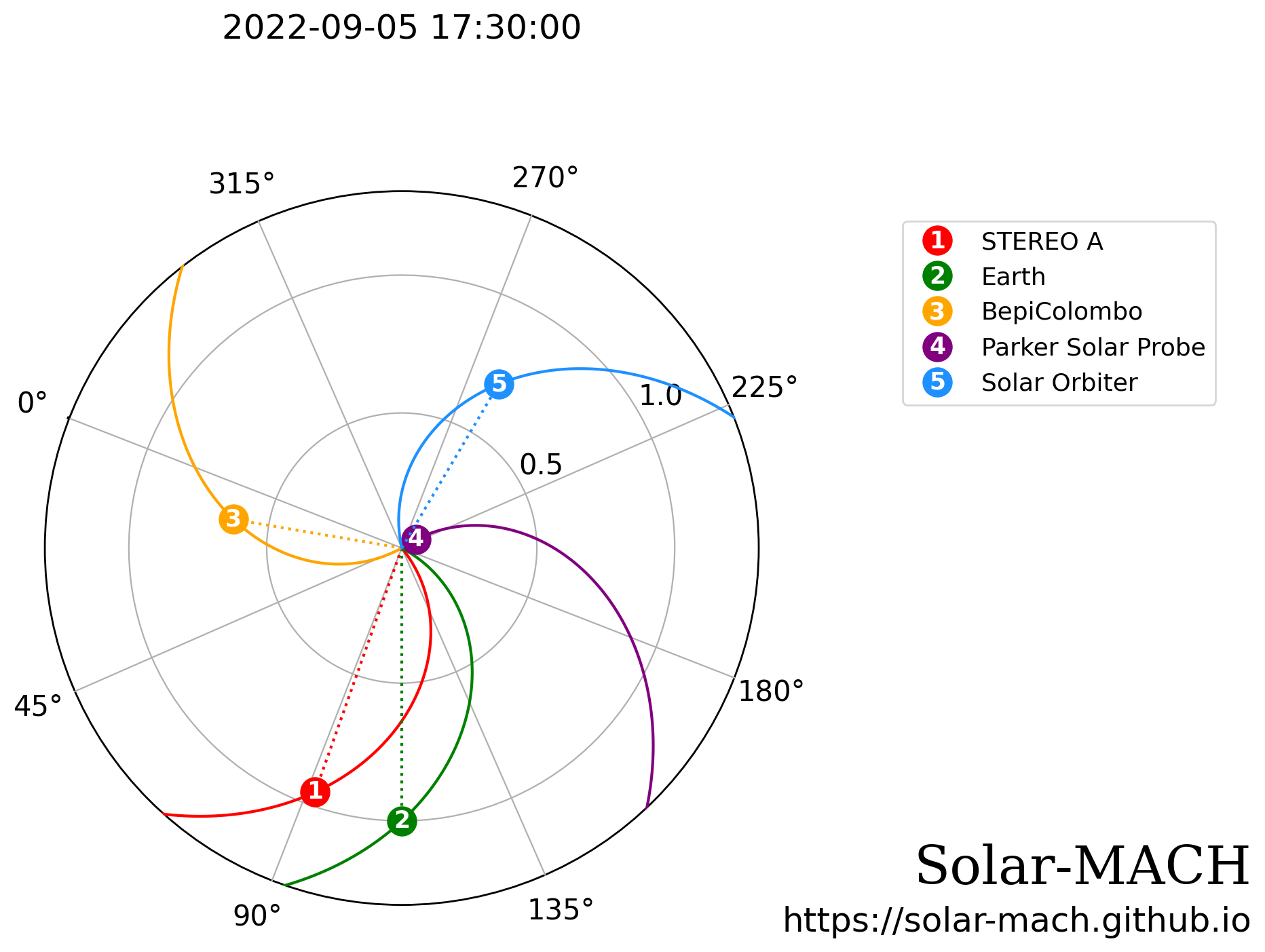
Figure 1: Spacecraft configuration at 17:30 UT of Sep. 05, 2022 (immediately after the IP shock crossed PSP). In this plot (generated using the Solar MAgnetic Connection HAUS tool  (Solar-MACH, Gieseler et al., 2023)), the Sun is at the center, the Earth is represented by the green circle, and the dashed (solid) lines indicate the spacecraft radial (along a Parker Spiral with a nominal speed of 400 km/s) connection.

3.1 Event Overview

On September 5, 2022, a CME erupted from the Sun and into interplanetary space. The CME was not Earth directed as the eruption happened on the far side of the Sun. An overview of the orbital configuration is shown in Figure 1.

A fast-forward shock, driven by the CME, was detected by PSP as close as 0.07 AU ($\sim$ 15 $\mathrm{R}_{\sun}$) at 17:27:19 UT, making this observation the closest to the Sun to date. An overview of the in-situ magnetic field and plasma quantities is shown on the left-hand side of Figure 2. A sharp transition in magnetic field, with a jump from about 600 to about 1600 nT occurs at the shock. The velocity profile across the shock transition shows two interesting features, namely a large flow speed deflection in the transverse direction $\mathrm{V_{T}}$, and a steady rise in $\mathrm{V_{R}}$ further downstream, up to about 17:35. We have marked this time as the end of the downstream (sheath) region of the event, i.e., the point where the leading edge of the CME flux rope likely starts (see also Romeo et al., 2023). However, we note that the boundary between the sheath and CME flux rope is not clear for this event. The properties of the CME sheath at such low heliocentric distances (and therefore early evolutionary stages) are very interesting and will be object of future work, comparing them with substructures and properties of CMEs at larger heliocentric distances (Kilpua et al., 2017).

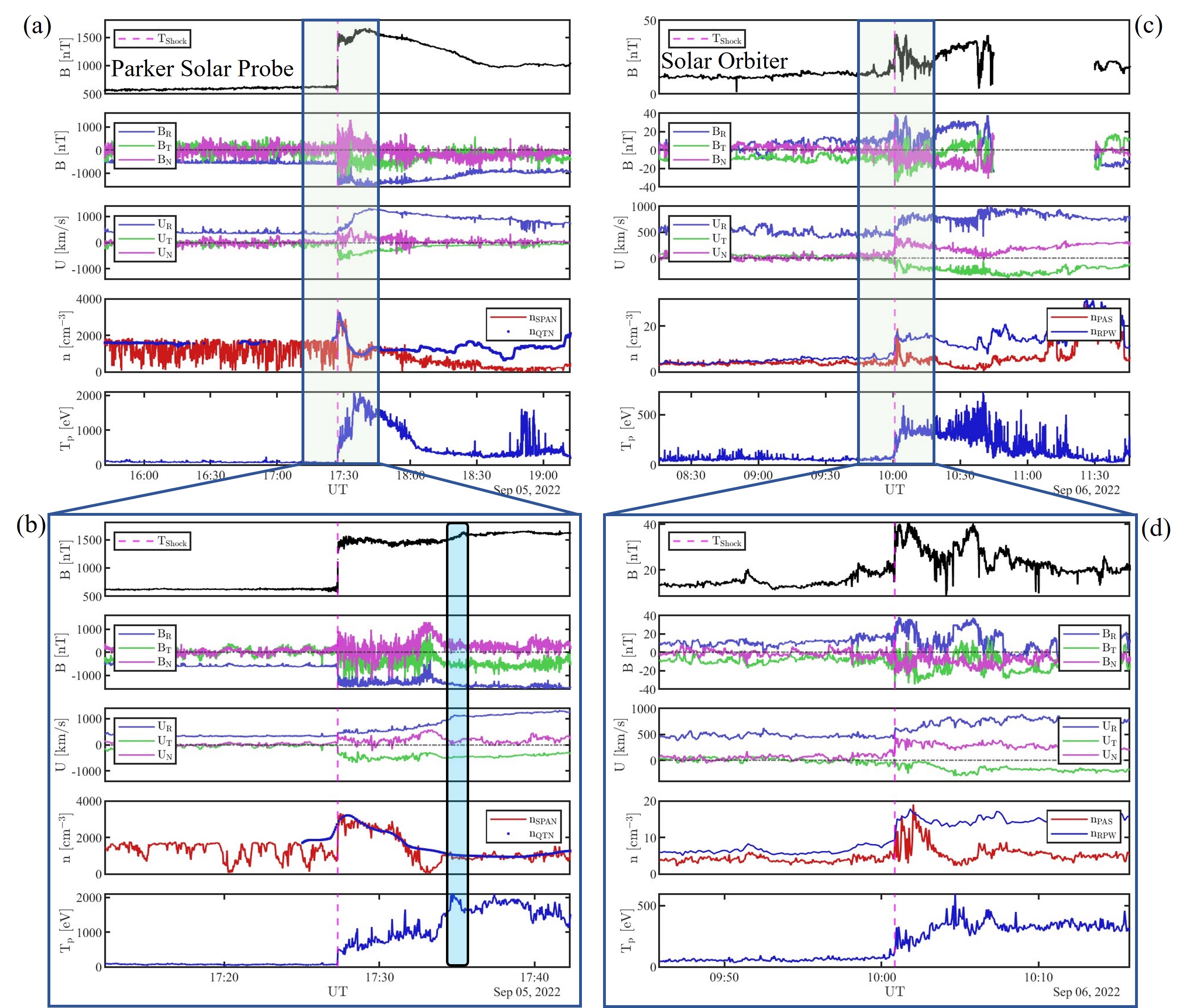
Figure 2: Magnetic field magnitude, its components in the RTN system, ion bulk flow velocity, density and temperature as measured by PSP (left) and later on by SolO (right). The plots show an overview of the event (a,c) with a zoom around the shock transition at both spacecraft (b,d). The dashed magenta line marks the shock transition, and the blue shaded area in panel (b) indicates the approximate end of the CME sheath as observed by PSP.

Table 1: In-situ shock parameters at PSP (left) and SolO (right). In the table are displayed, from top to bottom, the shock arrival time, Carrington longitude and latitude at the time of shock arrival, spacecraft heliocentric distance at the time of shock arrival, shock normal vector in $\mathrm{RTN}$ coordinates, shock normal angle $\langle\theta_{Bn}\rangle$, magnetic compression ratio $\langle\rm{r}_{B}\rangle$, gas compression ratio $\langle\rm{r}\rangle$, shock speed $v_{\mathrm{sh}}$, upstream plasma beta $\beta_{\mathrm{up}}$, fast magnetosonic and Alfvénic Mach numbers ($\rm{M_{\rm{fms}}}$ and $\rm{M_{\rm{A}}}$, respectively). The shock speed $v_{\mathrm{sh}}$ is along the shock normal and computed in the spacecraft rest frame using the mass flux conservation law.

	Parker Solar Probe	Solar Orbiter
Shock Time [UT]	05 Sep 2022, 17:27:19	06 Sep 2022, 10:00:51
Carrington longitude [∘]	232	251.9
Carrington latitude [∘]	-1.8	-3.6
Heliocentric dist. [AU]	0.07	0.7
$\langle\hat{\mathrm{n}}_{\mathrm{RTN}}\rangle$	[0.5 -0.8 0.2]	[0.6 -0.2 0.7]
$\langle\theta_{Bn}\rangle$ [∘]	53	51
$\langle\rm{r}_{B}\rangle$	2.3	1.9
$\langle\rm{r}\rangle$	1.6	2
$\langle v_{\rm{sh}}\rangle$ [km/s]	1520	942
$\beta_{\mathrm{up}}$	0.1	0.6
$\rm{M_{\rm{fms}}}$	3.8	3.2
$\rm{M_{\rm{A}}}$	3.9	3.8

We carried out a comprehensive characterization of the shock parameters locally observed by PSP. Given the density drops visible in the upstream region in Figure 2(b), due to the core of the ion distribution function not being well-inside the SPAN-i field of view (Livi et al., 2022), we estimated the density using the spacecraft quasi-thermal noise (QTN) for our shock analysis. Using a systematic collection of averaging windows spanning a few seconds to three minutes (with the technique described in Trotta et al. (2022a)) upstream/downstream of the shock, we used the Mixed Mode 3 method (MX3 Paschmann & Schwartz, 2000) to estimate the average shock normal $\langle n\rangle=[0.5,-0.8,0.2]$, though similar values are obtained with the other MX methods as well as magnetic coplanarity. Propagation direction deviating clearly from the radial direction is comptatible with the picture in which PSP is crossing a flank of the CME event. Our estimation of $\theta_{Bn}$ , i.e., the angle between the shock normal and the upstream magnetic field, a crucial parameter influencing shock behaviour, reveals that we are in the presence of an oblique ($\theta_{Bn}$ $\sim 53^{\circ}$), supercritical shock with moderate Alfvénic and fast magnetosonic Mach numbers ($\mathrm{M_{A}\simeq 3.9\,,\,M_{fms}\simeq 3.8}$, respectively) with respect to other IP shocks observed at or near 1 au (Kilpua et al., 2015). Furthermore, we find that the shock propagates at the very high speed of about 1500 km/s in the spacecraft frame and along the estimated shock normal. At PSP, upstream of the shock the magnetic field is mostly radial and interspersed with one-sided Alfvénic fluctuations (Gosling et al., 2009) of the magnetic field and ion bulk velocity, known as magnetic switchbacks, with angular deflections in the magnetic field of moderate amplitude, as expected for very low heliocentric distances (e.g. Jagarlamudi et al., 2023). SBs are a crucial feature of the solar wind in the inner heliosphere, as extensively shown in previous literature (Dudok de Wit et al., 2020; Krasnoselskikh et al., 2020; Larosa et al., 2021; Liang et al., 2021; Pecora et al., 2022; Liu et al., 2023; Jagarlamudi et al., 2023; Raouafi et al., 2023). Here, we have the opportunity to study how such structures are processed by shock waves, a crucial point of this work summarized in Section 3.2.

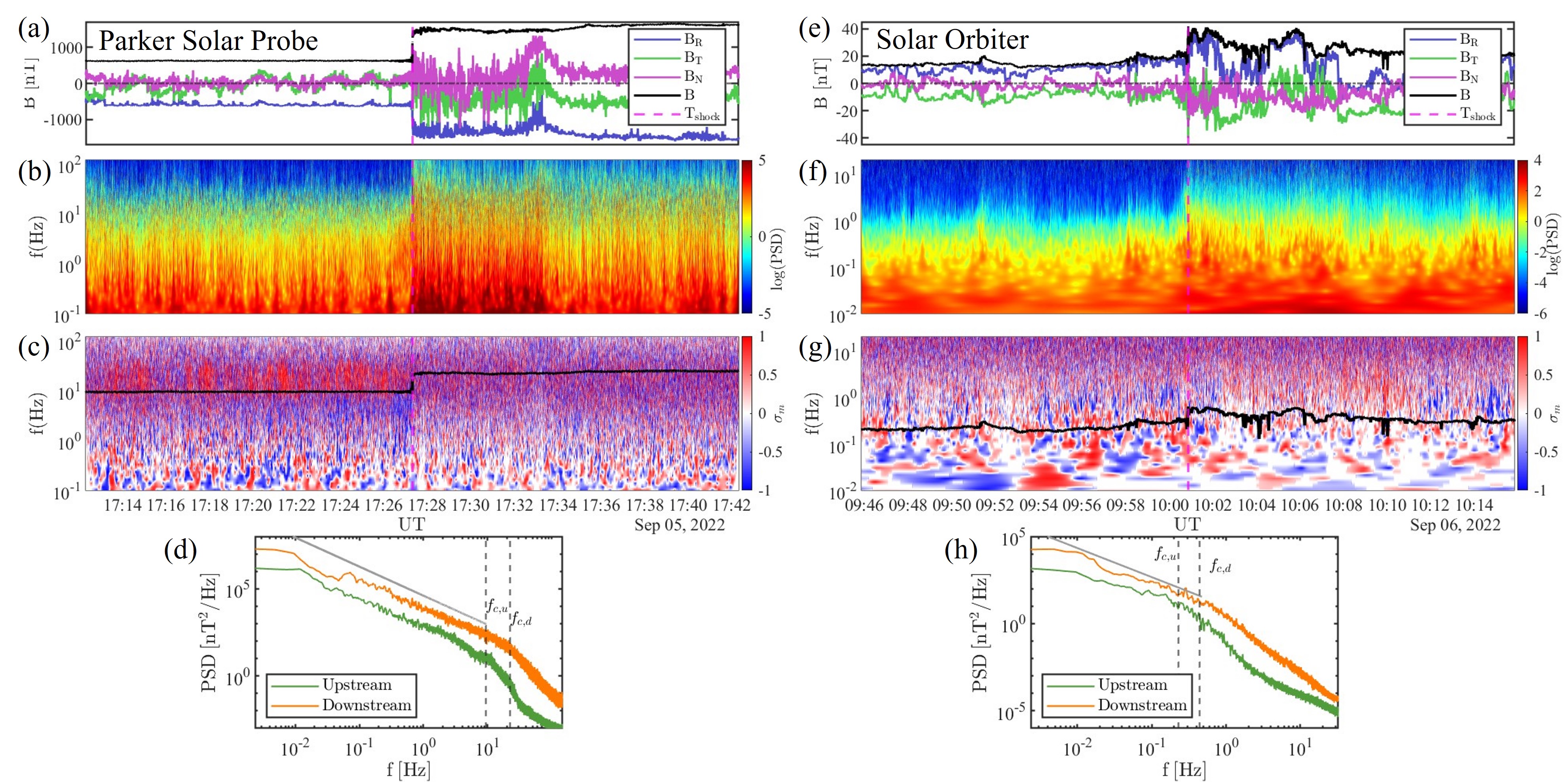
Figure 3: Magnetic fluctuations in the shock environment at PSP (left) and SolO (right). The Figure shows, from top to bottom: magnetic field magnitude and its components, trace wavelet spectrogram of the magnetic field (colormap), the normalised magnetic helicity $\sigma_{m}$ spectrogram, with the proton cyclotron frequency in the interval (black line), magnetic field power spectral densities (PSDs) computed in the 10 minutes upstream (green) and downstream (orange) of the shock.

At SolO (Fig. 2 right), the shock crossing appears much more structured compared to the PSP observation. Strong transverse flow deflections are still present, with a strong increase in $\mathrm{V_{N}}$ at the shock transition. The plasma density, as measured from the SWA-PAS and RPW instruments, yields two different values. For the shock parameter estimation, we used the density as measured by the RPW, since it is in agreement with the value obtained from EAS electron moments (Figure 8). However, locally computed shock parameters do not change dramatically when using the density derived from PAS. Steep upstream enhancements of magnetic field magnitude are found ahead of the shock (09:52, 09:56 UT), compatible with very rarely observed shocklets at strong IP shocks (Wilson et al., 2009; Trotta et al., 2023a). A high degree of magnetic field structuring is also found downstream of the shock, indicating a high level of complexity for this shock crossing. At SolO, the shock parameters estimation shows values very close to the ones observed at PSP (see Table 1). However, such values are obtained using very local averaging windows for the upstream/downstream quantities ($\sim$ 10 seconds to 1 minute). The overall behaviour of the shock at SolO indicates a high level of variability. Indeed, using larger averaging windows (about 6 to 10 minutes up/downstream), we find parameters compatible with a quasi-parallel shock transition ($\theta_{Bn}$ $\sim 30^{\circ}$) with high Mach numbers ($\mathrm{M_{A}\sim M_{fms}\sim 7}$). It is worth mentioning that, in addition to the local variability examined here, a different behaviour of the two shocks at PSP and SolO is expected, due to the crossing of the event at two different points in space and time. The longitudinal separation of PSP and SolO is of about 20^∘, and depending on the CME width, the shock will be crossed in different locations. However, such a comparison of shock parameters, summarized in Table 1, is useful when addressing the evolution of the whole event, and it may be important to support remote-sensing observations of the event as well as modelling of the CME evolution.

It is interesting, at this point, to characterize the environment in which the shock at PSP and SolO are propagating and how it is influenced by the shock passage. To this end, we studied the magnetic fluctuations in the $\sim$ 15 minutes before/after the shock arrival, with the relevant analyses shown in Figure 3.

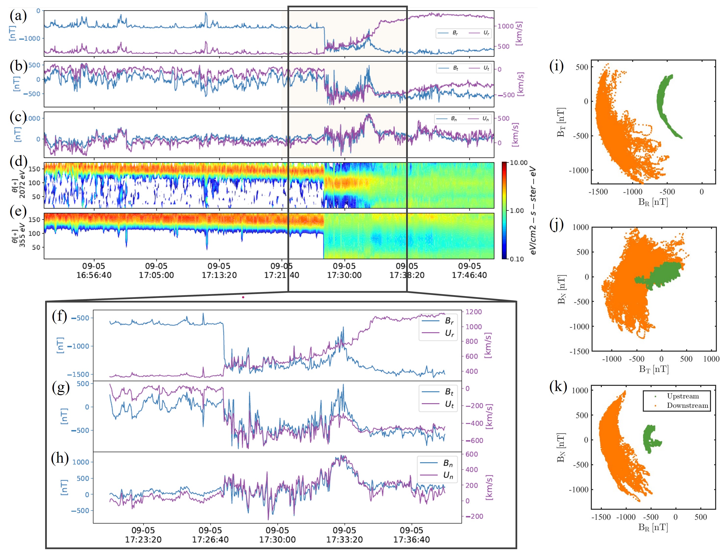
Figure 4: PSP observations of magnetic switchbacks transmission across the shock. (a) to (c): magnetic field (blue) and ion bulk flow velocity (plum) components. (d) and (e): pitch angle distributions for electrons with 2072 and 355 eV energy, respectively. (f) to (h): zoom around the shock crossing (shaded area in top panels). Scatterplots of radial and tangential (i), tangential and normal (j) and radial to normal (k) components of the magnetic field for the 4 minutes upstream of the shock crossing (green) and 4 minutes downstream of it (orange).

The shock crossing at PSP is characterized by a sharp transition, with no signs of upstream wave foreshock, as elucidated by the trace wavelet spectrogram in Figure 3(b). This is compatible with other observations of IP shocks, particularly at such oblique geometries (e.g. Blanco-Cano et al., 2016). It is worth noting that micro-instabilities of the shock front happening at ion kinetic scales, such as rippling (Trotta et al., 2023b) may still be present, albeit not well resolved by PSP. The level of magnetic fluctuations is enhanced in the downstream sheath region, lasting about 6 minutes. Such an enhancement in magnetic fluctuations is further shown in Figure 3(d), where the power spectral density in the 5 minutes upstream/downstream of the shock has been computed (green and orange lines, respectively). Here, it can be seen that the level of fluctuations increases by a factor of 4, and the downstream spectra show a flattening around the ion cyclotron frequency, a behaviour compatible with the spectral behaviour of IP shocks (Pitňa et al., 2021), with some observations of turbulence in the Earth’s bow shock environment (e.g. Sahraoui et al., 2020) and also compatible with modelling of turbulence transmission across shocks (see Fig. 18 in Zank et al., 2021). However, because the downstream flow speed is much larger than the upstream, and the shock changes the plasma parameters abruptly, the level of fluctuations may be overestimated. While the increase in the level of the frequency spectrum has been documented in previous literature (Zhao et al., 2021; Park et al., 2023), it remains to be understood if IP shocks inject new turbulence or they simply modify the background plasma properties. However, preliminary analysis shows that the spectral break happens around the ion skin depth $d_{i}$, compatible with statistical work carried out by Park et al. (2023). Further studies on the matter, relevant also for understanding the behaviour of turbulence at very low heliocentric distances (Zank et al., 2020) are further complicated by the geometrical constraints imposed by the single-spacecraft nature of the observations. These will be the objects of future work.

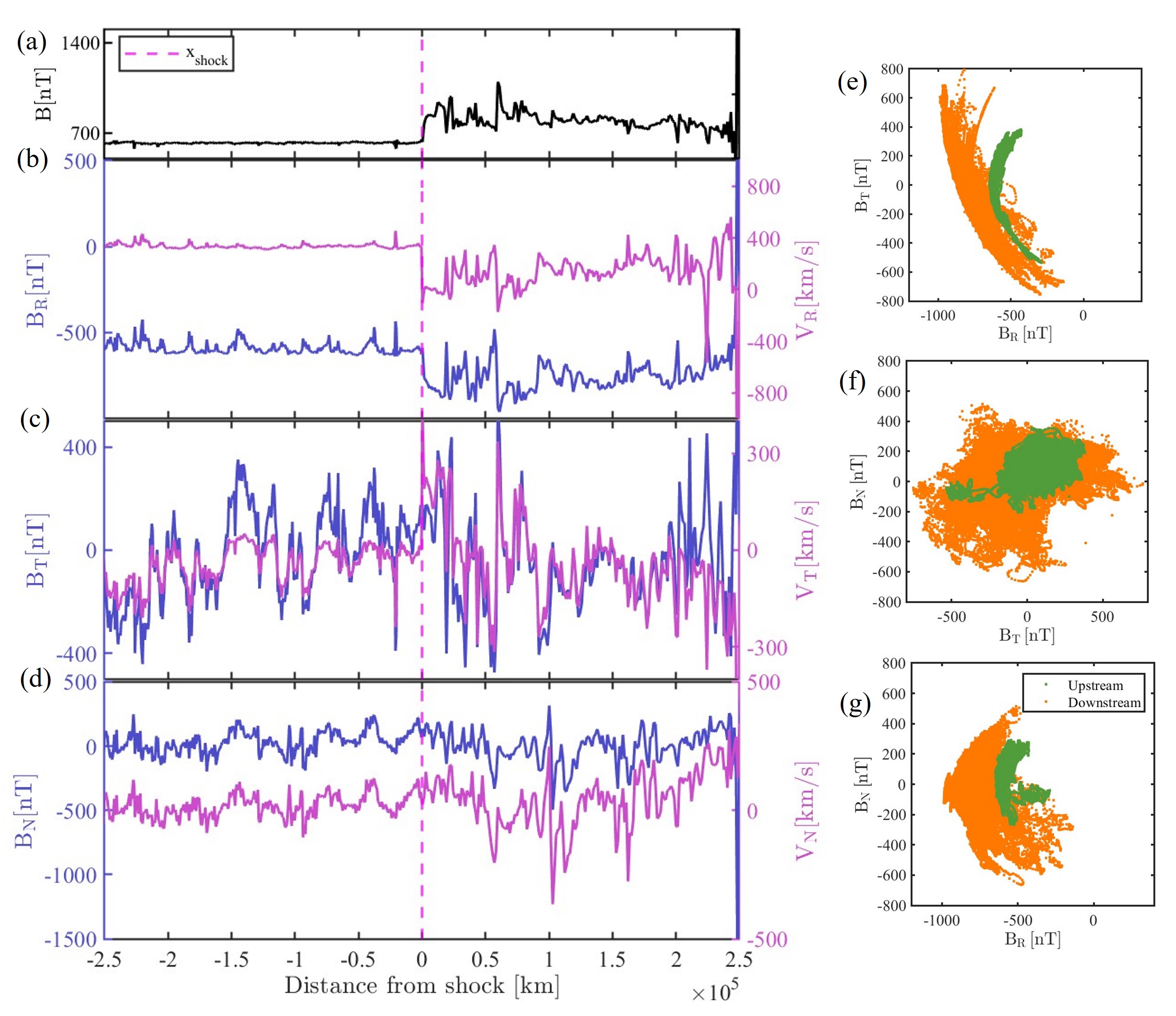
Figure 5: PSP observations of: (a)-(d): Magnetic field magnitude (black), magnetic field components (blue) and ion bulk flow speed components (plum) as a function of distance from the shock, where the downstream quantities have been decompressed using the Rankine-Hugoniot relations with the average shock parameters reported in Table 1. (e)-(g): Magnetic field excursion scatter plots as in Figure 4, performed on the decompressed quantities. Note that the scales in panels (e)-(g) are different from the ones used in Figure 4.

To further investigate the wave properties across the shock, we computed the normalised magnetic helicity, defined as

$$\sigma_{m}=\frac{2\Im\left(\tilde{B_{T}^{\star}}\tilde{B_{N}}\right)}{|\tilde{B_{R}}|^{2}+|\tilde{B_{T}}|^{2}+|\tilde{B_{N}}|^{2}},$$ (1)

where $\mathrm{B}$ indicates the magnetic field components, the $\tilde{}$ represents the wavelet- transformed quantities and $\star$ represents the complex conjugation operation (Matthaeus et al., 1982). Upstream of the shock at PSP, we observe a clear signature of consistently high $\sigma_{m}$ at ion scales, compatible with ion cyclotron wave activity (see the red patches by the ion plasma frequency line in Figure 3(c)). Ion cyclotron waves, crucial components of the solar wind as elucidated by PSP observations (Telloni et al., 2019; Verniero et al., 2020), have been shown to be very important for energy dissipation and solar wind heating (e.g. Woodham et al., 2018; Bowen et al., 2022). In our observations, we note that the magnetic helicity signature of ion cyclotron waves found upstream of the shock is lost in the shock downstream, as discussed in Section 3.2, together with an explanation of why such a behaviour is observed.

The magnetic fluctuations environment at SolO is different than that found at PSP (right-hand side of Figure 3). Here, the shock transition appears much more complex, especially due to the presence of larger scale structures at the SolO shock with respect to the PSP one. In the wavelet spectrum of the magnetic field, enhanced power extending to small ($\sim$ 1 Hz) scales is found corresponding to the upstream shocklet activity. The downstream appears populated with strong compressive and non compressive magnetic field fluctuations, indicative of the fact that the shock propagated through a very structured portion of the solar wind, as it can be noted from the magnetic field behaviour in the 10 minutes downstream of the shock (Blanco-Cano et al., 2019; Kropotina et al., 2021). The spectral behaviour of turbulence in being transmitted from the shock upstream to downstream is similar to the one observed for the shock at PSP, and compatible with previous multi- spacecraft studies of turbulence processed by IP shocks (Zhao et al., 2021). It is interesting to note that, in the IP case, an inertial range is always recovered downstream of IP shocks, in contrast with some observations of Earth’s magnetosheath where an inertial range is not observed downstream of Earth’s bow shock (Sahraoui et al., 2020), often interpreted as the Earth’s bow shock “resetting” the turbulent cascade. Finally, we note that some features of ion-cyclotron wave activity are seen upstream of the SolO event, though they are much less clear than the PSP observation.

3.2 The shock at Parker Solar Probe

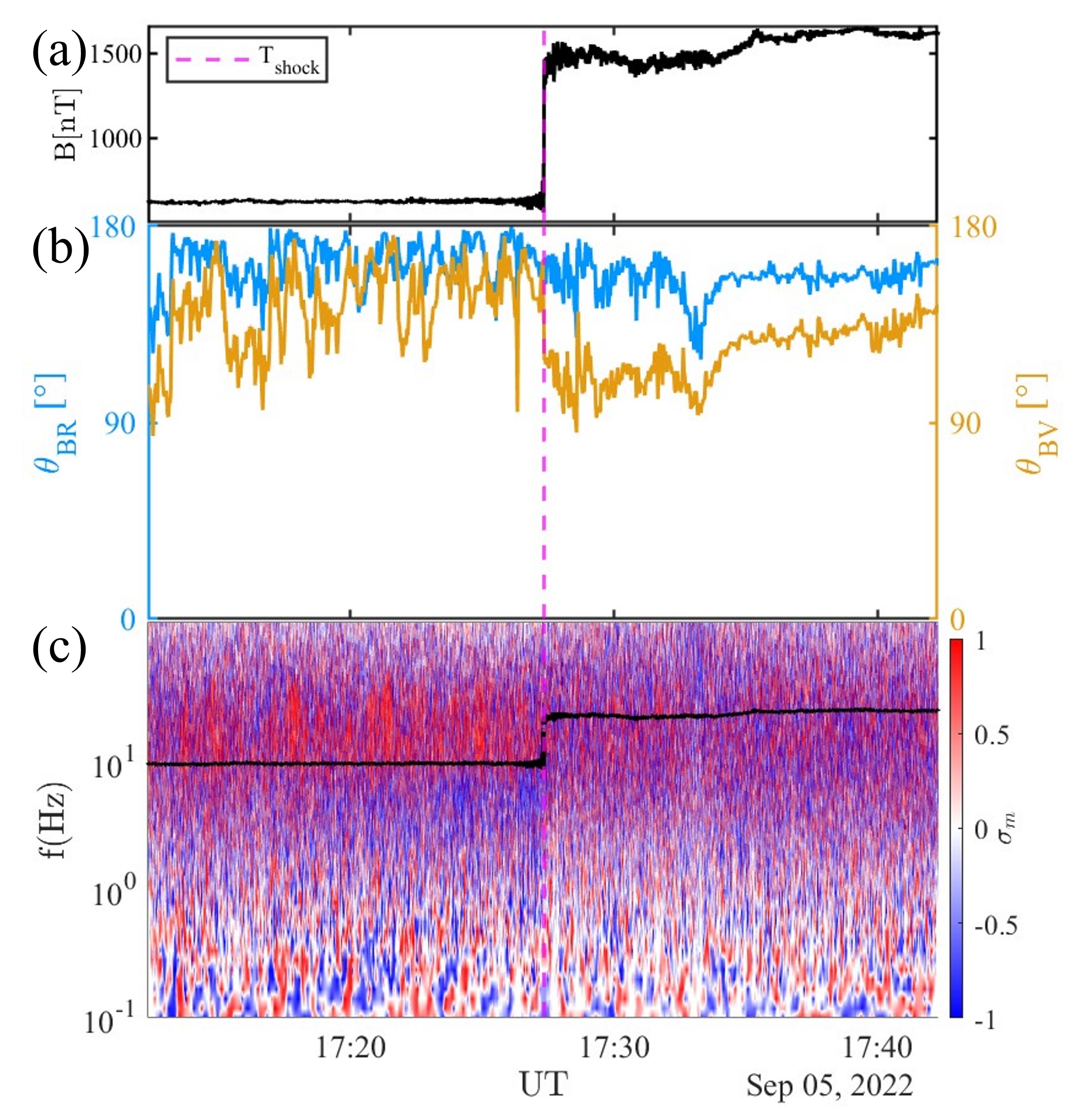
Figure 6: The IP shock interaction with ion cyclotron waves. (a): magnetic field magnitude around the shock crossing by PSP. (b) Angle between local magnetic field and radial direction ($\theta_{\mathrm{BR}}$ , blue) and ion velocity ($\theta_{\mathrm{BV}}$ , yellow). (c): Reduced magnetic helicity for the interval (as in Figure 3).

In this section, we focus on the PSP observations of the shock interacting with pre-existing fluctuations in the inner-heliospheric solar wind and its features. Particular interest is focused on how switchbacks (SBs) are processed by the IP shock wave.

In Figure 4 we observe the high degree of correlation between the magnetic and velocity fields. The presence of moderate amplitude SBs and their one-sided nature (Gosling et al., 2009), is evident especially in the $\mathrm{B_{R}}$ and $\mathrm{V_{R}}$ components (Figure 4(a)) upstream of the shock. In the downstream (sheath) region, the high degree of correlation is preserved, as elucidated by the Figure zoom (panels f, g, h). These observations reveal that the Alfvénic nature of the SBs is preserved downstream of the shock. However, the downstream SBs present larger, shock-driven variations in the field magnitude. Small deviations from a constant B state have been already observed at SBs boundaries (Krasnoselskikh et al., 2020; Farrell et al., 2020; Larosa et al., 2021). Here we show a different compressive effect, resulting from the propagation across the IP shock. As discussed in Section 3.1, the downstream region is characterized by stronger fluctuations driven by the shock, including small-scale, compressive fluctuations that are not Alfvénic.

From this point of view, it is interesting to note that the SBs signature is not completely lost upon shock passage, but rather the SBs are processed by the shock. Considering the Rankine-Hugoniot relations describing the change in plasma parameters across MHD shocks (e.g. Krehl, 2015), we expect, for the SBs, a compression along the shock normal direction, and a stretch along the two shock transverse directions. The extremely short duration of the sheath poses a strong limitation on a more quantitative study of how SB are affected by the shock. For instance, the Z parameter would be helpful in addressing such an issue (Dudok de Wit et al., 2020). Such an investigation will be carried out in future works focusing on several shocks at low heliocentric distances.

To further investigate how the shock affects the upstream SBs, we study the magnetic field excursion in the regions upstream and downstream of the shock (Figure 4(i-m)), as done in other studies elucidating the nature of fluctuations in the solar wind (e.g., Matteini et al., 2015). Two effects arise in the magnetic field fluctuations after the shock crossing. First of all, due the change in background field magnitude, the arc of polarization upon which the magnetic field fluctuates become wider, as particularly evident in the $\mathrm{B_{R}}$-$\mathrm{B_{T}}$ scatter plot (Figure 4(i)). It is also possible to observe that downstream magnetic field fluctuations cover a larger area in the magnetic field excursion space, due to the presence of compressive fluctuations in the shock downstream. From Figure 4(i-j-k), it is possible to note that the arc of polarization is displaced from the R-T plane into both the R-T and R-N plane when comparing the shock upstream to the downstream, consistent with compression along the normal and the stretching along the perpendicular directions. The shock-SBs interaction may have important consequences for the SBs’ ability to propagate without dispersive effects, and therefore it may affect the SBs lifetime, since the constant B magnitude is a necessary condition for the unperturbed propagation of large amplitude Alfvén waves (Barnes & Hollweg, 1974).

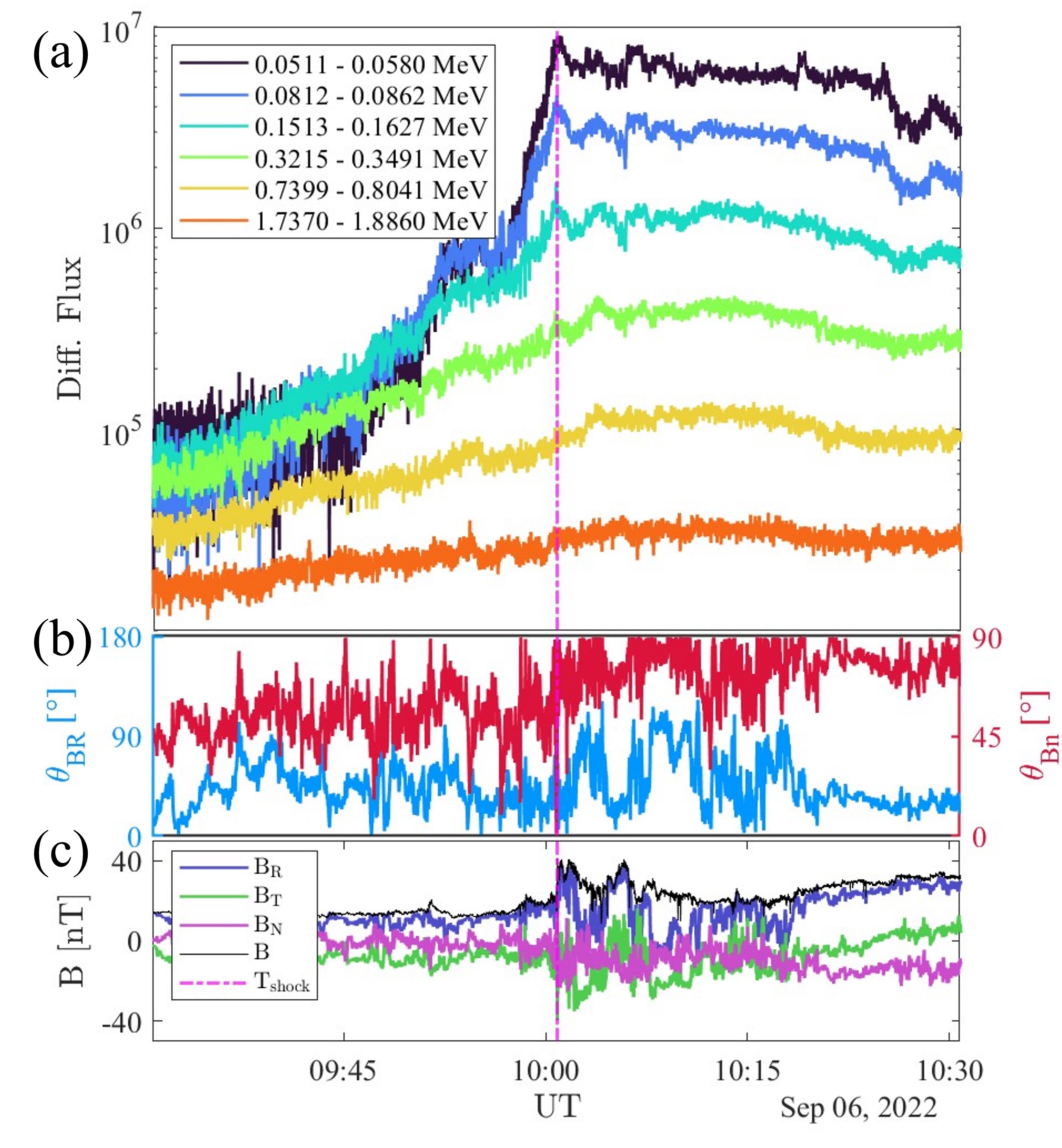
Figure 7: (a): Energetic ion fluxes in the $\sim$0.05 - 2 MeV energy range as observed by the Sun telescope of EPD-EPT instrument of Solar Orbiter. (b): Local $\theta_{\mathrm{BR}}$ (blue) and $\theta_{Bn}$ (red) angles. (c) Magnetic field magnitude (black) and its components. The dashed magenta line indicates the shock crossing time.

The above assessment of the SBs features upstream/downstream of the shock suffers from limitations related to the single-spacecraft nature of the observations. First, it is known that the features of SBs (deflections, duration) tend to have broad distributions (e.g., Larosa et al., 2021), making it difficult to estimate the extent to which the processed, downstream SBs were comparable to their upstream, unshocked counterparts before they crossed the shock. Furthermore, how plasma is sampled by PSP throughout the observation introduces a geometrical constraint on the observations, where fluctuations are sampled differently from upstream to downstream. This latter point is further expanded in Figure 6(b) and related discussion. Another crucial caveat stems from the downstream flow speed in the spacecraft frame being much larger than that upstream, allowing more plasma to flow over the spacecraft per unit time, causing the downstream SBs to appear shorter than their upstream counterparts, an effect that appears in addition to the compression induced by the shock. Furthermore, the field increase due to the presence of the shock influences the discussion of the downstream SBs deflection amplitude (Figure 4(i)).

For this reason, we decided to “unshock” the magnetic field and plasma time series across the PSP shock crossing. This analysis is carried out in two steps. First, using the mean upstream and downstream flow speeds, we plot the PSP measurements in units of distance from shock using the Taylor hypothesis (Taylor, 1938). Then, we used the Rankine-Hugoniot jump conditions to remove the shock compression. Here, knowing the downstream quantities and the shock parameters as estimated from the spacecraft crossing (see Table 1), we derived the upstream quantities, i.e., we estimated the magnetic field and plasma conditions prior to the shock passage. Further details about this method of decompression can be found in the Appendix A. The resulting, decompressed timeseries is shown in Figure 5. As can be seen in panels (a)-(d), the jump in the magnetic field and speed is greatly reduced with this technique. It is possible to see that, some compression in magnetic field persists even after the plasma has been “unshocked”. This is due to the decompression method having several limitations. First, the shock parameters are assumed to be fixed throughout the decompression, and are estimated using a single spacecraft technique, inherently affected by uncertainties (Trotta et al., 2022a). The shock variability, particularly important for supercritical shocks, on a variety of scales (e.g. Marghitu et al., 2017; Kajdič et al., 2019, 2021) may therefore introduce fluctuations in the decompression. Finally, as discussed in the appendix, the decompression method makes use of the Rankine-Hugoniot jump conditions without including waves and/or turbulence (e.g., Zank et al., 2002; Gedalin, 2023). This technique can be further improved, in future studies, to mitigate the above limitations.

The preservation of the SBs Alfvénicity is evident from Figure 5 (a)-(d), where the downstream behaviour of the magnetic field and velocity fluctuations is remarkably similar to the upstream one. The analysis of magnetic field excursions further strengthens this point, where compatible behaviour between downstream and upstream fluctuations is found. The magnetic field excursion space covered by the downstream fluctuations is still larger, due to some compressive features downstream of the shock not fully removed by the Rankine-Hugoniot decompression. However, we observe that downstream of the shock we find larger deflections of the magnetic field. It is also worth noting that, after decompression, the difference in the $\mathrm{B_{R}}$-$\mathrm{B_{N}}$ plane becomes less evident.

A totally different behaviour from that found for SBs is found for the upstream ion cyclotron waves discussed in Section 3.1. The signature of these waves, a clearly visible feature in the reduced magnetic helicity spectrogram (red patches of $\sigma_{m}=1$, near ion plasma frequency, Figure 3), is completely lost downstream of the shock. We address this interesting feature in Figure 6, where we study how PSP crosses the wave environment surrounding the shock. To this end, we compute the angle between the local magnetic field and the radial direction, $\theta_{\mathrm{BR}}$, and the angle between the local magnetic field and the local velocity $\theta_{\mathrm{BV}}$, where $\mathbf{V}=\mathbf{V}-\mathbf{V_{PSP}}$, where $\mathbf{V}_{\mathbf{PSP}}$ is the velocity of PSP in the inertial RTN frame. In Figure 6(b) ion cyclotron waves are clearly observed when $\theta_{\mathrm{BV}}$ is close to 180 degrees and lost when $\theta_{\mathrm{BV}}$ is of the order of 90 degrees. This behaviour could be simply due to an observational bias. As shown by  Bowen et al. (2020), this phenomenon is the result of measuring a quasi-parallel wave vector at oblique angles combined with the higher amplitude in the perpendicular direction of the anisotropic turbulent fluctuations. Furthermore, the conditions downstream of the shock inhibit the possibility of resonant beam-field interaction, due to the strongly turbulent environment diffusing the beam in velocity space (e.g., Valentini et al., 2010). We analysed the ion velocity distribution functions as measured by SPANi, albeit their being complicated by the limited field of view of the instrument, we did not find any beam signature downstream of the shock, suggesting that the production mechanisms of ion cyclotron waves are indeed suppressed. A detailed investigation of such features is out of scope for this work and will be the object of further studies.

3.3 The shock at Solar Orbiter

In this Section, we discuss the event as observed by SolO. The shock crossed the spacecraft at 10:00:51 on Sep 6, 2022. The shock parameters, reported in Table 1, are compatible with the PSP observations. However, as discussed in Section 3.1, shock variability plays a major role in the SolO observations. Here, the shock transition appears far more structured, with an overall behaviour compatible with strong shocks.

Such interesting aspects of the SolO shock observations are investigated in Figure 7. The structuring observed in the shock surroundings is particularly evident in the 20 minutes downstream of the shock, populated with many sharp changes of magnetic field (Figure 7). First of all, using the EPD-EPT instrument, we address how the production of energetic particles is affected by such disturbed conditions. As can be seen in Figure 7(a), energetic ions of up to $\sim$ 2 MeV are accelerated by the shock, with fluxes rising as the shock crossing is approached, a behaviour typical of ion acceleration at IP shocks (Giacalone, 2012; Lario et al., 2022). Interestingly, some of the fluxes (e.g. the ones for $\sim$0.33 and $\sim$ 0.7 MeV, green and yellow lines, respectively) have their peak at a time which is not coincident with the shock crossing time at SolO, but instead is downstream of the shock. This behaviour, consistent with the statistical study presented in Lario et al. (2003), has implications on the production and propagation of shock accelerated particles (Perri et al., 2022), and may well be due to additional acceleration mechanisms downstream of the shock (Zank et al., 2015; Zhao et al., 2018; Kilpua et al., 2023).

A crucial feature found for the energetic particle population is the fluctuations found in their fluxes immediately downstream of the shock with typical timescales of 1 to 2 minutes, particularly evident for the lower energy channels (0.05 to 0.35 MeV, dark blue to green). Such fluctuations correlate well with the magnetic field structuring (Figure 7(a)-(c)), thus suggesting that particle acceleration is indeed happening in an irregular fashion for this IP shock, where additional acceleration may be provided by the magnetic structures (Zhao et al., 2018; Trotta et al., 2022b; Nakanotani et al., 2021). To quantify the variability associated with the shock crossing, the $\theta_{Bn}$ and local $\theta_{\mathrm{BR}}$ angles have been estimated using the local magnetic field, the radial direction and the average shock normal as reported in Table 1. It is evident from this analysis, shown in in Figure 7(b), that the shock geometry changes significantly on the timescales examined here, moving from quasi-perpendicular to quasi-parallel geometries and thus supporting the picture of irregular particle acceleration. Complementing the theme of shock variability, it is worth discussing the role of plasma structures in particle acceleration. The typical gyroradii of the particles showing such irregular behaviour have been estimated using the local magnetic field, $\mathrm{r}_{L}\sim 10^{4}$ km. Using the Taylor’s hypothesis, such lengths compare to 1/10th of the typical size of the downstream structures, thus suggesting that trapping of accelerated particles may play a role into the variability observed in the particle fluxes, an important source of extra particle acceleration beyond the shock (see Zank et al., 2015; Zhao et al., 2018; Trotta et al., 2020; Roux et al., 2019; Pezzi et al., 2022).

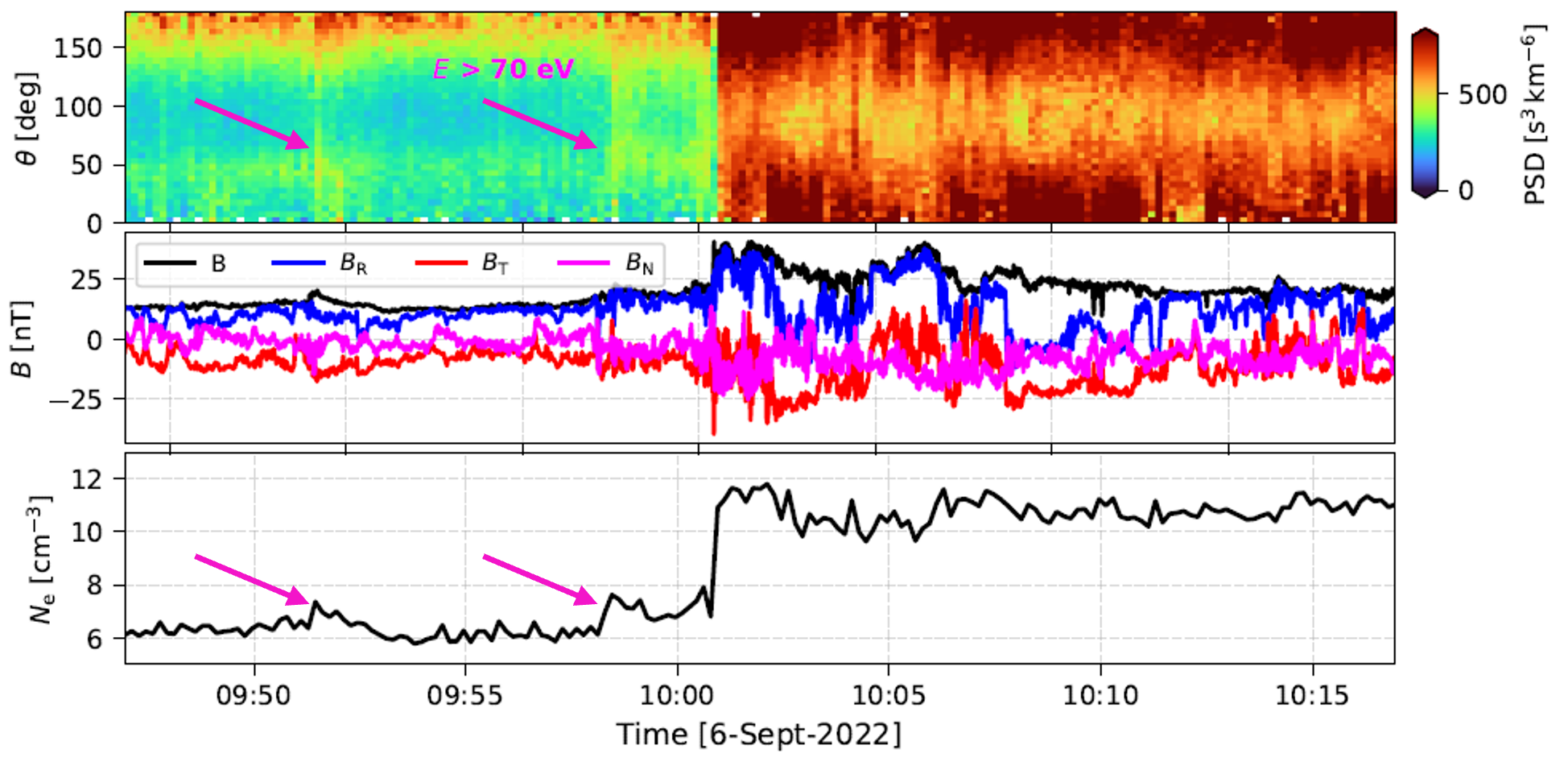
Figure 8: Overview of electron behaviour at SolO. Top: EAS electron pitch angle distributions for particles with energy larger than 70 eV. Middle: Magnetic field measurements in RTN.Bottom: electron density computed from EAS measurements.

Another extremely interesting feature of the SolO observations is the steep magnetic field enhancements observed in the 10 minutes upstream of the shock (Figure 8). Such steep enhancements are compatible with upstream shocklets, typically arising from the interplay between shock-reflected, energetic ions and upstream waves which, in the case of Earth’s bow shock, are the Ultra Low Frequency (ULF) waves routinely found in the foreshock (Stasiewicz et al., 2003). Shocklets are important as they influence the plasma environment upstream of the shock transition, thus pre-conditioning the shock inflow (Lucek et al., 2008). Most of our knowledge of shocklets is built on observations upstream of Earth’s bow shock (Plaschke et al., 2018), being rarely observed at IP shocks with only three cases previously reported (Lucek & Balogh, 1997; Wilson et al., 2009; Trotta et al., 2023a), making this observation particularly interesting.

Two shocklets were observed upstream of the shock at SolO, compatible with the fact that, when estimated at $\sim$ 20 minute timescales, the shock Mach number is high and the geometry quasi-parallel (see discussion in Section 3.1). In Figure 8, we show how the shocklets influence the low-energy electron population using SolO-EAS measurements. First of all, shocklets are associated with rises in the electron density, identified by the magenta arrows in Figure 8(c), a behaviour recently found also at Venus (Collinson et al., 2023). Furthermore, by analysing the pitch-angle distributions of electrons with energy greater than 70 eV, we found that electrons are more isotropic in pitch angle space in the vicinity of the shocklets, probably due to pitch-angle scattering induced by the compressive structures, as observed in the Earth’s bow shock environment (Wilson III et al., 2013). This behaviour, namely the pre-conditioning of the upstream particle population, may have important consequences for electron injection and acceleration to higher energies (Katou & Amano, 2019; Dresing et al., 2022; Wijsen et al., 2023).

4 Conclusions

The September 05, 2022 CME event provided an opportunity to study a CME-driven IP shock at unprecedentedly low heliocentric distance, with PSP crossing the event at 0.07 au. Furthermore, well-radially aligned SolO at 0.7 au provided important insights about the evolution of the event.

We focused on the small-scale behaviour of CME-driven shocks associated with this event. The PSP spacecraft observed the shock very early in its evolution. The shock had moderate Mach numbers ($\mathrm{M_{A}}\sim\mathrm{M_{fms}}\sim 4)$), as inferred using local shock parameter estimation. The average shock normal was found to be $\mathrm{\hat{n}}=(0.5,-0.8,0.2)$, significantly departing from the radial direction, indicating that the crossing of the shock likely happened on one flank of the CME event. This has also important implications when addressing the joint PSP-SolO observations, as due the shock will be crossed in different loactions, with features depending on the CME width and spacecraft longitudinal separation. The shock at PSP has a notably short sheath region due to its early evolutionary stage, an interesting property that may have fundamental implications for the possibility of accelerating particles to high energies, as preliminary shown in Cohen et al. (2023). We however emphasize that as this event was crossed at the flanks of the sheath - CME flux rope boundary cannot be determined accurately.

We studied how switchbacks, fundamental constituents of the solar wind as elucidated by several, previous PSP observations (e.g. Bale et al., 2019; Kasper et al., 2019; Dudok de Wit et al., 2020), are processed in the shock crossing. We found that the SBs are compressed along the shock normal direction and stretched along the other two directions. Interestingly, many SBs properties are preserved in the shock downstream. Furthermore, SBs with larger magnetic field deflections were found in the shock downstream, an important ingredient to consider when addressing their statistical properties. Such statistical properties of how SBs are processed by IP shocks will be object of future investigation, now increasingly possible thanks to the novel PSP ShOck Detection Algorithm (SODA) IP shock list https://parker.gsfc.nasa.gov/shocks.html. This behaviour has been investigated in detail by looking at the decompressed magnetic field and plasma quantities, obtained using the Rankine-Hugoniot shock jump conditions. This technique of decompression is useful to estimate how quantities were before their interaction with the shock. It can also be used to yield an estimate of how the ambient plasma conditions could change due to the passage of a shock with a given set of parameters, as will be shown in future work.

How ion cyclotron waves are transmitted across the shock was also addressed. This study is particularly interesting due to the role that ion cyclotron waves play for energy dissipation (e.g., Bowen et al., 2022). We observe that the signature of pre-existing ion cyclotron waves, identified in the shock upstream at PSP, disappears downstream of the shock (Figure 6). This may be due to the sudden change in plasma conditions at the shock, injecting strong fluctuations in the downstream, making the conditions for ion cyclotron waves propagation less favourable. Through the analysis of the $\theta_{\mathrm{BV}}$ and $\theta_{\mathrm{BR}}$ angles, we also found unfavourable conditions to detecting ion cyclotron activity downstream (Bowen et al., 2020), due to the change of the mean magnetic field direction upon the shock passage.

SolO observations of the same event are extremely interesting to address the role of evolution for the CME shock region in its propagation to larger heliocentric distances. On the large scales, we note that the large transverse flow deflections are still present, with a $\mathrm{V_{N}}$ increase comparable to the one observed in $\mathrm{V_{R}}$.

The shock environment at SolO is much more disturbed than the one observed at PSP. A shock parameter estimation using very short averaging windows ($\sim$ 1 minute, thus addressing the very local shock properties) yields similar values with respect to the PSP observations (see Table 1). However, analysing the 30 minutes across the shock transition, we find an environment compatible with a quasi-parallel shock and relatively high Mach number, propagating in a very structured portion of the solar wind. Two shocklets, structures that grow favourably upstream of high Mach number, quasi-parallel shocks, were found upstream of the shock, a rare observation for the interplanetary case. Signature of $\sim 100$ eV electrons scattering was found corresponding to the shocklets, an important ingredient to be considered for pre-conditioning of the upstream particle population at the shock. It is worth noting that these shocklets, with duration much larger than those observed at Earth’s bow shock, probably arise from pre-existing upstream waves and not from shock-generated upstream waves, a behaviour observed also for the case in  Trotta et al. (2023a). Therefore, this observation points to the idea that the origin of the IP shocklets is different than those observed in the Earth’s foreshock.

Energetic ions up to 2 MeV were found in association with the shock at SolO. A detailed analysis of the high time resolution EPD-EPT energetic particle fluxes reveal structuring corresponding to the magnetic field structures processed by the shock, indicating a potential role of trapping as an extra source of energy for particle acceleration.

Finally, we underline that this event is a very good example of the novel observational window provided by missions exploring the inner heliosphere such as PSP and SolO, exploited in this study to highlight the fact that the features of IP shock environments can be very different as they propagate through the heliosphere, with important consequences on the modelling effort accuracy and possibility of prediction associated with such energetic events.

5 acknowledgments

This work has received funding from the European Unions Horizon 2020 research and innovation programme under grant agreement No. 101004159 (SERPENTINE, www.serpentine-h2020.eu). AL is supported by STFC Consolidated Grant ST/T00018X/1. CHKC is supported by UKRI Future Leaders Fellowship MR/W007657/1 and STFC Consolidated Grants ST/T00018X/1 and ST/X000974/1. H.H. is supported by the Royal Society University Research Fellowship URF/R1/180671. N.D. is grateful for support by the Academy of Finland (SHOCKSEE, grant No. 346902). The PSP/FIELDS experiment was developed and is operated under NASA contract NNN06AA01C. Work at IRAP is supported by CNRS, UPS, and CNES.E.E.D acknowledges funding by the European Union (ERC, HELIO4CAST, 101042188). Views and opinions expressed are however those of the author(s) only and do not necessarily reflect those of the European Union or the European Research Council Executive Agency. Neither the European Union nor the granting authority can be held responsible for them. XBC is grateful to PAPIIT DGAPA grant IN110921. This work was supported by the UK Science and Technology Facilities Council (STFC) grant ST/W001071/1.L.F. .is supported by the Royal Society University Research Fellowship No. URF\R1\231710. RFWS thanks the German Space Agency (DLR) for its support of SOLO/EPD under grant 50OT2002.

Appendix A Rankine-Hugoniot decompression method

Heliospheric shocks crossing spacecraft can be directly measured. An hypothesis that is often made when interpreting spacecraft measurements is the Taylor hypothesis (Taylor, 1938), linking time-variations in the spacecraft measured quantities to spatial variations. Thus, upon shock crossing, it is possible to address the properties of the upstream/downstream shock environments (see Figure 2). However, it is often the case that it would be interesting to address the shock downstream plasma before it was shocked, as discussed in Section 3.2. Here we present a technique providing a proxy to address the plasma condition before the shock propagation.

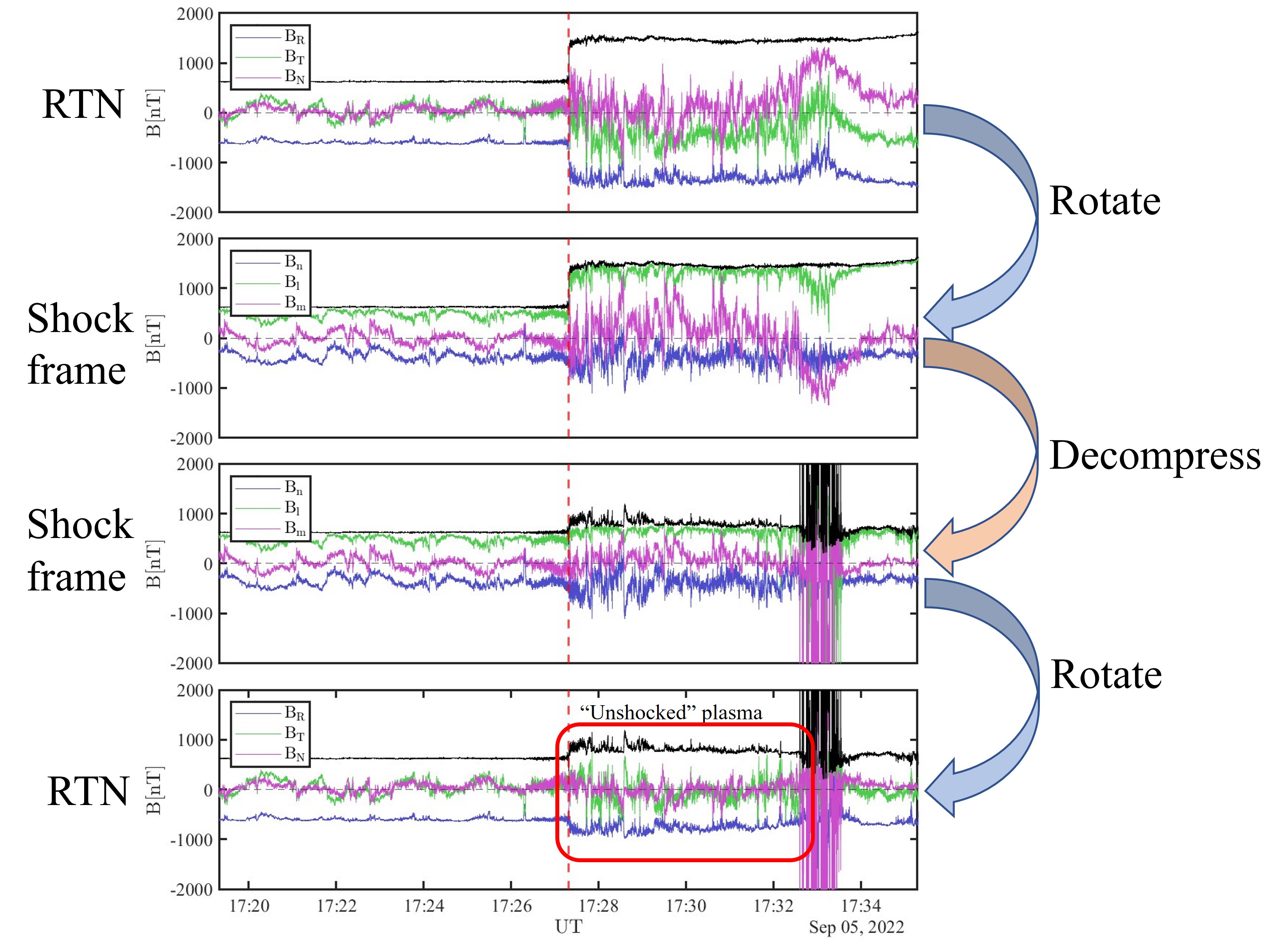
Figure 9: Overview of the procedure of magnetic field decompression.

The Rankine-Hugoniot jump conditions (e.g., Burgess & Scholer, 2015) have been widely used to model the plasma properties across a shock. Here, the shock is treated as a planar, one-dimensional, time stationary structure. Following an integration of the MHD equations for mass, momentum and energy conservation, and the divergence-free condition for the magnetic field, the Rankine-Hugoniot relations linking the properties of upstream and downstream plasmas can be written as follows:

$$\frac{\rho_{m2}}{\rho_{m1}} =\mathrm{r_{gas}}$$ (A1)

$$\frac{V_{n2}}{V_{n1}} =\frac{1}{\mathrm{r_{gas}}}$$ (A2)

$$\frac{V_{t2}}{V_{t1}} =\frac{M^{2}_{A1}-1}{M^{2}_{A1}-\mathrm{r_{gas}}}$$ (A3)

$$\frac{B_{n2}}{B_{n1}} =1$$ (A4)

$$\frac{B_{t2}}{B_{t1}} =\mathrm{r_{gas}}\frac{M^{2}_{A1}-1}{M^{2}_{A1}-\mathrm{r_{gas}}}$$ (A5)

$$\frac{P_{2}}{P_{1}} =\mathrm{r_{gas}}+\frac{(\gamma-1)\mathrm{r_{gas}}V_{1}^{2}}{2V_{S}1}\left(1-\frac{V_{2}^{2}}{V_{1}^{2}}\right).$$ (A6)

The above equations for density, bulk flow velocity, magnetic field and pressure ($\rho_{m},V,B$ and $P$, respectively) are expressed in the deHoffmann-Teller frame, i.e., a frame aligned to the shock normal that moves at a speed such that the upstream convective electric field ($\mathbf{E}_{1}=-\mathbf{V}_{1}\times\mathbf{B}_{1}$) vanishes (de Hoffmann & Teller, 1950). Here, the subscripts 1 and 2 are referred to the upstream and downstream states, respectively. The subscripts $n$ and $t$, instead, indicate the shock normal and tangential directions. $\mathrm{r_{gas}}$ is the shock gas compression ratio, and $M_{A1}\equiv V_{n1}\sqrt{\mu_{0}\rho_{m1}}/B_{n1}$ is the Alfvénic Mach number. $V_{S1}$ is the upstream sound speed.

Often, the Rankine-Hugoniot equations are used to address shock parameters. What we do in our decompression technique is instead to use the downstream measurements and the shock parameters to compute the upstream conditions, thus “unshocking” the plasma according to Equations A1-A6. The procedure, given a time-series of spacecraft measurements, is performed as follows, and displayed in Figure 9. First, the data is rotated in a shock normal frame. Here, we choose the $nlm$ frame, where the $n$ direction is aligned with the shock normal (computed using the MX3 method (Paschmann & Schwartz, 2000)), $m$ is perpendicular both to the shock normal and to the upstream magnetic field, and $l$ completes the triad. A boost is performed to then move to the deHoffman-Teller frame. Then, Equations A1-A6 are used to derive the upstream quantities given the downstream measurements and the shock parameters, i.e., the decompression is performed. The data is then returned in the spacecraft frame. Finally, using the mean upstream and downstream flow speeds, it is possible to shock the measurements in units of distance from shock (see Figure 5).

This technique, while giving a proxy for the plasma conditions before shock processing, has several limtations. The decompression is performed assuming that the shock parameters do not change throughout the event, thus neglecting the inherent variability of shock system. Shock parameters are estimated from single spacecraft measurements, and therefore are associated to uncertainties. The Rankine-Hugoniot relations used to decompress the plasma assume a one-dimensional, planar, time-stationary MHD shock with laminar upstream/downstream regions, which is notoriously a stringent assumption for heliosphere shocks, that are characterised by several space/time variabilities and propagate in the turbulent solar wind.

For the above reasons, it is readily understood that the decompression is more reliable for closer measurements with respect to the shock crossing. In Figure 9, it is possible to see how unphysical results are introduced by the large structure embedded in the plasma happening around 17:33 UT. Future improvements of the diagnostic for example including wave transmission will be object of future work.

References

- Adhikari et al. (2022) Adhikari, L., Zank, G. P., Telloni, D., & Zhao, L.-L. 2022, The Astrophysical Journal Letters, 937, L29, doi: 10.3847/2041-8213/ac91c6
- Bale et al. (2016) Bale, S. D., Goetz, K., Harvey, P. R., et al. 2016, Space Sci. Rev., 204, 49, doi: 10.1007/s11214-016-0244-5
- Bale et al. (2019) Bale, S. D., Badman, S. T., Bonnell, J. W., et al. 2019, Nature, 576, 237, doi: 10.1038/s41586-019-1818-7
- Bale et al. (2023) Bale, S. D., Drake, J. F., McManus, M. D., et al. 2023, Nature, 618, 252, doi: 10.1038/s41586-023-05955-3
- Barnes & Hollweg (1974) Barnes, A., & Hollweg, J. V. 1974, J. Geophys. Res., 79, 2302, doi: 10.1029/JA079i016p02302
- Blanco-Cano et al. (2019) Blanco-Cano, X., Burgess, D., Sundberg, T., & Kajdič, P. 2019, Journal of Geophysical Research: Space Physics, 124, 9760, doi: https://doi.org/10.1029/2019JA026748
- Blanco-Cano et al. (2016) Blanco-Cano, X., Kajdič, P., Aguilar-Rodríguez, E., et al. 2016, Journal of Geophysical Research: Space Physics, 121, 992, doi: https://doi.org/10.1002/2015JA021645
- Bowen et al. (2020) Bowen, T. A., Mallet, A., Huang, J., et al. 2020, ApJS, 246, 66, doi: 10.3847/1538-4365/ab6c65
- Bowen et al. (2022) Bowen, T. A., Chandran, B. D. G., Squire, J., et al. 2022, Phys. Rev. Lett., 129, 165101, doi: 10.1103/PhysRevLett.129.165101
- Burgess & Scholer (2015) Burgess, D., & Scholer, M. 2015, Collisionless Shocks in Space Plasmas (Cambridge University Press), doi: 10.1017/CBO9781139044097
- Burton et al. (1992) Burton, M. E., Smith, E. J., Goldstein, B. E., et al. 1992, Geophysical Research Letters, 19, 1287, doi: https://doi.org/10.1029/92GL01284
- Bykov et al. (2019) Bykov, A. M., Vazza, F., Kropotina, J. A., Levenfish, K. P., & Paerels, F. B. S. 2019, Space Sci. Rev., 215, 14, doi: 10.1007/s11214-019-0585-y
- Cohen et al. (2023) Cohen, C., Christian, E., Cummings, A. C., et al. 2023, PoS, ICRC2023, 1276, doi: 10.22323/1.444.1276
- Collinson et al. (2023) Collinson, G. A., Hietala, H., Plaschke, F., et al. 2023, Geophysical Research Letters, 50, e2023GL104610, doi: https://doi.org/10.1029/2023GL104610
- de Hoffmann & Teller (1950) de Hoffmann, F., & Teller, E. 1950, Physical Review, 80, 692, doi: 10.1103/PhysRev.80.692
- Dessler & Fejer (1963) Dessler, A. J., & Fejer, J. A. 1963, Planetary and Space Science, 11, 505, doi: 10.1016/0032-0633(63)90074-6
- Dresing et al. (2023) Dresing, Rodríguez-García, L., Jebaraj, I. C., et al. 2023, A&A, 674, A105, doi: 10.1051/0004-6361/202345938
- Dresing et al. (2022) Dresing, N., Kouloumvakos, A., Vainio, R., & Rouillard, A. 2022, The Astrophysical Journal Letters, 925, L21, doi: 10.3847/2041-8213/ac4ca7
- Dudok de Wit et al. (2020) Dudok de Wit, T., Krasnoselskikh, V. V., Bale, S. D., et al. 2020, ApJS, 246, 39, doi: 10.3847/1538-4365/ab5853
- Dungey (1979) Dungey, J. W. 1979, Nuovo Cimento C Geophysics Space Physics C, 2C, 655, doi: 10.1007/BF02558123
- Eastwood et al. (2015) Eastwood, J. P., Hietala, H., Toth, G., et al. 2015, Space Sci Rev, 188, 251, doi: 10.1007/s11214-014-0050-x
- Farrell et al. (2020) Farrell, W. M., MacDowall, R. J., Gruesbeck, J. R., Bale, S. D., & Kasper, J. C. 2020, ApJS, 249, 28, doi: 10.3847/1538-4365/ab9eba
- Fox et al. (2016) Fox, N. J., Velli, M. C., Bale, S. D., et al. 2016, Space Sci. Rev., 204, 7, doi: 10.1007/s11214-015-0211-6
- Gedalin (2023) Gedalin, M. 2023, The Astrophysical Journal, 958, 2, doi: 10.3847/1538-4357/ad0461
- Giacalone (2005) Giacalone, J. 2005, ApJ, 628, L37, doi: 10.1086/432510
- Giacalone (2012) Giacalone, J. 2012, The Astrophysical Journal, 761, 28, doi: 10.1088/0004-637X/761/1/28
- Giacalone et al. (2021) Giacalone, J., Burgess, D., Bale, S. D., et al. 2021, The Astrophysical Journal, 921, 102, doi: 10.3847/1538-4357/ac1ce1
- Gieseler et al. (2023) Gieseler, J., Dresing, N., Palmroos, C., et al. 2023, Frontiers in Astronomy and Space Sciences, 9, doi: 10.3389/fspas.2022.1058810
- Gosling et al. (1974) Gosling, J. T., Hildner, E., MacQueen, R. M., et al. 1974, Journal of Geophysical Research, 79, 4581, doi: 10.1029/JA079I031P04581
- Gosling et al. (2009) Gosling, J. T., McComas, D. J., Roberts, D. A., & Skoug, R. M. 2009, ApJ, 695, L213, doi: 10.1088/0004-637X/695/2/L213
- Guo et al. (2021) Guo, F., Giacalone, J., & Zhao, L. 2021, Frontiers in Astronomy and Space Sciences, 8, doi: 10.3389/fspas.2021.644354
- Horbury et al. (2020) Horbury, T. S., O’Brien, H., Carrasco Blazquez, I., et al. 2020, Astronomy & Astrophysics, 642, A9, doi: 10.1051/0004-6361/201937257
- Jagarlamudi et al. (2023) Jagarlamudi, V. K., Raouafi, N. E., Bourouaine, S., et al. 2023, The Astrophysical Journal Letters, 950, L7, doi: 10.3847/2041-8213/acd778
- Kajdič et al. (2019) Kajdič, P., Preisser, L., Blanco-Cano, X., Burgess, D., & Trotta, D. 2019, ApJ, 874, L13, doi: 10.3847/2041-8213/ab0e84
- Kajdič et al. (2021) Kajdič, P., Pfau-Kempf, Y., Turc, L., et al. 2021, Journal of Geophysical Research: Space Physics, 126, e2021JA029283, doi: https://doi.org/10.1029/2021JA029283
- Kasper et al. (2016) Kasper, J. C., Abiad, R., Austin, G., et al. 2016, Space Sci. Rev., 204, 131, doi: 10.1007/s11214-015-0206-3
- Kasper et al. (2019) Kasper, J. C., Bale, S. D., Belcher, J. W., et al. 2019, Nature, 576, 228, doi: 10.1038/s41586-019-1813-z
- Katou & Amano (2019) Katou, T., & Amano, T. 2019, ApJ, 874, 119, doi: 10.3847/1538-4357/ab0d8a
- Khotyaintsev et al. (2021) Khotyaintsev, Graham, D. B., Vaivads, A., et al. 2021, A&A, 656, A19, doi: 10.1051/0004-6361/202140936
- Kilpua et al. (2017) Kilpua, E., Koskinen, H. E. J., & Pulkkinen, T. I. 2017, Living Reviews in Solar Physics, 14, 5, doi: 10.1007/s41116-017-0009-6
- Kilpua et al. (2023) Kilpua, E., Vainio, R., Cohen, C., et al. 2023, Ap&SS, 368, 66, doi: 10.1007/s10509-023-04201-6
- Kilpua et al. (2015) Kilpua, E. K., Lumme, E., Andreeova, K., Isavnin, A., & Koskinen, H. E. 2015, Journal of Geophysical Research: Space Physics, 120, 4112, doi: 10.1002/2015JA021138
- Krasnoselskikh et al. (2020) Krasnoselskikh, V., Larosa, A., Agapitov, O., et al. 2020, ApJ, 893, 93, doi: 10.3847/1538-4357/ab7f2d
- Krehl (2015) Krehl, P. O. K. 2015, European Physical Journal H, 40, doi: 10.1140/epjh/e2015-50010-4
- Kropotina et al. (2021) Kropotina, J. A., Webster, L., Artemyev, A. V., et al. 2021, The Astrophysical Journal, 913, 142, doi: 10.3847/1538-4357/abf6c7
- Lai et al. (2012) Lai, H. R., Russell, C. T., Jian, L. K., et al. 2012, Sol. Phys., 278, 421, doi: 10.1007/s11207-012-9955-2
- Lario et al. (2003) Lario, D., Ho, G. C., Decker, R. B., et al. 2003, AIP Conference Proceedings, 679, 640, doi: 10.1063/1.1618676
- Lario et al. (2022) Lario, D., Richardson, I. G., Wilson, L. B., I., et al. 2022, ApJ, 925, 198, doi: 10.3847/1538-4357/ac3c47
- Larosa et al. (2021) Larosa, A., Krasnoselskikh, V., Dudok de Wit, T., et al. 2021, A&A, 650, A3, doi: 10.1051/0004-6361/202039442
- Liang et al. (2021) Liang, H., Zank, G. P., Nakanotani, M., & Zhao, L.-L. 2021, The Astrophysical Journal, 917, 110, doi: 10.3847/1538-4357/ac0a73
- Liu et al. (2023) Liu, Y. D., Ran, H., Hu, H., & Bale, S. D. 2023, ApJ, 944, 116, doi: 10.3847/1538-4357/acb345
- Livi et al. (2022) Livi, R., Larson, D. E., Kasper, J. C., et al. 2022, The Astrophysical Journal, 938, 138, doi: 10.3847/1538-4357/ac93f5
- Long et al. (2023) Long, D. M., Green, L. M., Pecora, F., et al. 2023, The Astrophysical Journal, 955, 152, doi: 10.3847/1538-4357/acefd5
- Lucek & Balogh (1997) Lucek, E. A., & Balogh, A. 1997, Geophysical Research Letters, 24, 2387, doi: 10.1029/97GL52471
- Lucek et al. (2008) Lucek, E. A., Horbury, T. S., Dandouras, I., & Rème, H. 2008, Journal of Geophysical Research: Space Physics, 113, doi: https://doi.org/10.1029/2007JA012756
- Maksimovic, M. et al. (2020) Maksimovic, M., Bale, S. D., Chust, T., et al. 2020, A&A, 642, A12, doi: 10.1051/0004-6361/201936214
- Marghitu et al. (2017) Marghitu, O., Comişel, H., & Scholer, M. 2017, Geophysical Research Letters, 44, 6500, doi: https://doi.org/10.1002/2017GL073241
- Matteini et al. (2015) Matteini, L., Horbury, T. S., Pantellini, F., Velli, M., & Schwartz, S. J. 2015, The Astrophysical Journal, 802, 11, doi: 10.1088/0004-637X/802/1/11
- Matthaeus et al. (1982) Matthaeus, W. H., Goldstein, M. L., & Smith, C. 1982, Phys. Rev. Lett., 48, 1256, doi: 10.1103/PhysRevLett.48.1256
- McComas et al. (2023) McComas, D. J., Sharma, T., Christian, E. R., et al. 2023, The Astrophysical Journal, 943, 71, doi: 10.3847/1538-4357/acab5e
- Moncuquet et al. (2020) Moncuquet, M., Meyer-Vernet, N., Issautier, K., et al. 2020, The Astrophysical Journal Supplement Series, 246, 44, doi: 10.3847/1538-4365/ab5a84
- Müller et al. (2020) Müller, St. Cyr, O. C., Zouganelis, I., et al. 2020, A&A, 642, A1, doi: 10.1051/0004-6361/202038467
- Nakanotani et al. (2021) Nakanotani, M., Zank, G. P., & Zhao, L.-L. 2021, The Astrophysical Journal, 922, 219, doi: 10.3847/1538-4357/ac2e06
- Nakanotani et al. (2022) —. 2022, The Astrophysical Journal, 926, 109, doi: 10.3847/1538-4357/ac4781
- Nicolaou et al. (2021) Nicolaou, Wicks, R. T., Owen, C. J., et al. 2021, A&A, 656, A10, doi: 10.1051/0004-6361/202140875
- Owen et al. (2020) Owen, C. J., Bruno, R., Livi, S., et al. 2020, Astronomy & Astrophysics, 642, doi: 10.1051/0004-6361/201937259
- Park et al. (2023) Park, B., Pitňa, A., Šafránková, J., et al. 2023, The Astrophysical Journal Letters, 954, L51, doi: 10.3847/2041-8213/acf4ff
- Paschmann & Schwartz (2000) Paschmann, G., & Schwartz, S. J. 2000, ESA Special Publication, Vol. 449, ISSI Book on Analysis Methods for Multi-Spacecraft Data, ed. R. A. Harris, 99
- Pecora et al. (2022) Pecora, F., Matthaeus, W. H., Primavera, L., et al. 2022, ApJ, 929, L10, doi: 10.3847/2041-8213/ac62d4
- Pérez-Alanis et al. (2023) Pérez-Alanis, C. A., Janvier, M., Nieves-Chinchilla, T., et al. 2023, Sol. Phys., 298, 60, doi: 10.1007/s11207-023-02152-3
- Perri et al. (2022) Perri, S., Bykov, A., Fahr, H., Fichtner, H., & Giacalone, J. 2022, Space Sci. Rev., 218, 26, doi: 10.1007/s11214-022-00892-5
- Pezzi et al. (2022) Pezzi, O., Blasi, P., & Matthaeus, W. H. 2022, ApJ, 928, 25, doi: 10.3847/1538-4357/ac5332
- Pitna et al. (2023) Pitna, A., Zank, G. P., Nakanotani, M., et al. 2023, Journal of Physics: Conference Series, 2544, 012009, doi: 10.1088/1742-6596/2544/1/012009
- Pitňa et al. (2017) Pitňa, A., Šafránková, J., Němeček, Z., & Franci, L. 2017, ApJ, 844, 51, doi: 10.3847/1538-4357/aa7bef
- Pitňa et al. (2021) Pitňa, A., Šafránková, J., Němeček, Z., Ďurovcová, T., & Kis, A. 2021, Frontiers in Physics, 8, doi: 10.3389/fphy.2020.626768
- Plaschke et al. (2018) Plaschke, F., Hietala, H., Archer, M., et al. 2018, Space Science Reviews, 214, doi: 10.1007/S11214-018-0516-3
- Raouafi et al. (2023) Raouafi, N. E., Matteini, L., Squire, J., et al. 2023, Space Sci. Rev., 219, 8, doi: 10.1007/s11214-023-00952-4
- Reames (1999) Reames, D. V. 1999, Space Sci. Rev., 90, 413, doi: 10.1023/A:1005105831781
- Richardson (2018) Richardson, I. G. 2018, Living Reviews in Solar Physics, 15, 1, doi: 10.1007/s41116-017-0011-z
- Richardson (2011) Richardson, J. D. 2011, Journal of Atmospheric and Solar-Terrestrial Physics, 73, 1385, doi: https://doi.org/10.1016/j.jastp.2010.06.005
- Rodríguez-Pacheco et al. (2020) Rodríguez-Pacheco, Wimmer-Schweingruber, R. F., Mason, G. M., et al. 2020, A&A, 642, A7, doi: 10.1051/0004-6361/201935287
- Romeo et al. (2023) Romeo, O. M., Braga, C. R., Badman, S. T., et al. 2023, The Astrophysical Journal, 954, 168, doi: 10.3847/1538-4357/ace62e
- Roux et al. (2019) Roux, J. A. L., Webb, G. M., Khabarova, O. V., Zhao, L.-L., & Adhikari, L. 2019, The Astrophysical Journal, 887, 77, doi: 10.3847/1538-4357/ab521f
- Sahraoui et al. (2020) Sahraoui, F., Hadid, L., & Huang, S. 2020, Reviews of Modern Plasma Physics, 4, 4, doi: 10.1007/s41614-020-0040-2
- Schwartz et al. (2022) Schwartz, S. J., Goodrich, K. A., Wilson III, L. B., et al. 2022, Journal of Geophysical Research: Space Physics, 127, doi: https://doi.org/10.1029/2022JA030637
- Stasiewicz et al. (2003) Stasiewicz, K., Longmore, M., Buchert, S., et al. 2003, Geophysical Research Letters, 30, doi: https://doi.org/10.1029/2003GL017971
- Sundberg et al. (2016) Sundberg, T., Haynes, C. T., Burgess, D., & Mazelle, C. X. 2016, The Astrophysical Journal, 820, 21, doi: 10.3847/0004-637X/820/1/21
- Taylor (1938) Taylor, G. I. 1938, Proceedings of the Royal Society of London Series A, 164, 476, doi: 10.1098/rspa.1938.0032
- Telloni et al. (2019) Telloni, D., Carbone, F., Bruno, R., et al. 2019, The Astrophysical Journal Letters, 885, L5, doi: 10.3847/2041-8213/ab4c44
- Trotta et al. (2020) Trotta, D., Franci, L., Burgess, D., & Hellinger, P. 2020, ApJ, 894, 136, doi: 10.3847/1538-4357/ab873c
- Trotta et al. (2023a) Trotta, D., Hietala, H., Horbury, T., et al. 2023a, Monthly Notices of the Royal Astronomical Society, 520, 437, doi: 10.1093/mnras/stad104
- Trotta et al. (2021) Trotta, D., Valentini, F., Burgess, D., & Servidio, S. 2021, Proceedings of the National Academy of Sciences, 118, e2026764118, doi: 10.1073/pnas.2026764118
- Trotta et al. (2022a) Trotta, D., Vuorinen, L., Hietala, H., et al. 2022a, Frontiers in Astronomy and Space Sciences, 9, doi: 10.3389/fspas.2022.1005672
- Trotta et al. (2022b) Trotta, D., Pecora, F., Settino, A., et al. 2022b, The Astrophysical Journal, 933, 167, doi: 10.3847/1538-4357/ac7798
- Trotta et al. (2023b) Trotta, D., Pezzi, O., Burgess, D., et al. 2023b, Monthly Notices of the Royal Astronomical Society, 525, 1856, doi: 10.1093/mnras/stad2384
- Turc et al. (2023) Turc, L., Roberts, O. W., Verscharen, D., et al. 2023, Nature Physics, 19, 78, doi: 10.1038/s41567-022-01837-z
- Valentini et al. (2010) Valentini, F., Iazzolino, A., & Veltri, P. 2010, Physics of Plasmas, 17, 052104, doi: 10.1063/1.3420278
- Verniero et al. (2020) Verniero, J. L., Larson, D. E., Livi, R., et al. 2020, ApJS, 248, 5, doi: 10.3847/1538-4365/ab86af
- Webb & Howard (2012) Webb, D. F., & Howard, T. A. 2012, Living Reviews in Solar Physics, 9, 3, doi: 10.12942/lrsp-2012-3
- Wijsen et al. (2023) Wijsen, N., Lario, D., Sánchez-Cano, B., et al. 2023, The Astrophysical Journal, 950, 172, doi: 10.3847/1538-4357/acd1ed
- Wilkinson (2003) Wilkinson, W. P. 2003, Planetary and Space Science, 51, 629, doi: https://doi.org/10.1016/S0032-0633(03)00099-0
- Wilson et al. (2009) Wilson, L. B. I., Cattell, C. A., Kellogg, P. J., et al. 2009, Journal of Geophysical Research: Space Physics, 114, doi: https://doi.org/10.1029/2009JA014376
- Wilson III et al. (2013) Wilson III, L. B., Koval, A., Sibeck, D. G., et al. 2013, Journal of Geophysical Research: Space Physics, 118, 957, doi: https://doi.org/10.1029/2012JA018186
- Woodham et al. (2018) Woodham, L. D., Wicks, R. T., Verscharen, D., & Owen, C. J. 2018, The Astrophysical Journal, 856, 49, doi: 10.3847/1538-4357/aab03d
- Yang et al. (2023) Yang, L., Heidrich-Meisner, V., Berger, L., et al. 2023, Astronomy & Astrophysics, in press
- Zank et al. (2020) Zank, G. P., Nakanotani, M., Zhao, L.-L., Adhikari, L., & Telloni, D. 2020, The Astrophysical Journal, 900, 115, doi: 10.3847/1538-4357/abad30
- Zank et al. (2021) Zank, G. P., Nakanotani, M., Zhao, L. L., et al. 2021, The Astrophysical Journal, 913, 127, doi: 10.3847/1538-4357/abf7c8
- Zank et al. (2002) Zank, G. P., Zhou, Y., Matthaeus, W. H., & Rice, W. K. M. 2002, Physics of Fluids, 14, 3766, doi: 10.1063/1.1507772
- Zank et al. (2015) Zank, G. P., Hunana, P., Mostafavi, P., et al. 2015, ApJ, 814, 137, doi: 10.1088/0004-637X/814/2/137
- Zhao et al. (2021) Zhao, Zank, G. P., He, J. S., et al. 2021, A&A, 656, A3, doi: 10.1051/0004-6361/202140450
- Zhao et al. (2018) Zhao, L.-L., Zank, G. P., Khabarova, O., et al. 2018, The Astrophysical Journal Letters, 864, L34, doi: 10.3847/2041-8213/aaddf6