FM-G-CAM: A Holistic Approach for Explainable AI in Computer Vision

Abstract

Explainability is an aspect of modern AI that is vital for impact and usability in the real world. The main objective of this paper is to emphasise the need to understand the predictions of Computer Vision models, specifically Convolutional Neural Network (CNN) based models. Existing methods of explaining CNN predictions are mostly based on Gradient-weighted Class Activation Maps (Grad-CAM) and solely focus on a single target class. We show that from the point of the target class selection, we make an assumption on the prediction process, hence neglecting a large portion of the predictor CNN model’s thinking process. In this paper, we present an exhaustive methodology called Fused Multi-class Gradient-weighted Class Activation Map (FM-G-CAM) that considers multiple top predicted classes, which provides a holistic explanation of the predictor CNN’s thinking rationale. We also provide a detailed and comprehensive mathematical and algorithmic description of our method. Furthermore, along with a concise comparison of existing methods, we compare FM-G-CAM with Grad-CAM, highlighting its benefits through real-world practical use cases. Finally, we present an open-source Python library with FM-G-CAM implementation to conveniently generate saliency maps for CNN-based model predictions.

Keywords Explainable AI  $\cdot$ Computer Vision  $\cdot$ Image Classification

1 Introduction

Explainability is an aspect of Artificial Intelligence (AI) that is gaining prominence today. Explainable AI (XAI) enables humans to more comprehensively understand model predictions as opposed to black box approaches, which is of paramount importance for the use of such technologies in the real world[1, 2, 3]. Among many other fields, computer vision is a field that often benefits from XAI, in part due to its visual nature [4, 5, 2]. In the field of Computer Vision, both Convolutional Neural Networks (CNNs) and Transformer-based models are widely used for image classification[6, 7, 8]. It is worth noting that several transformer-based approaches use convolutional layers.

Despite the strengths of CNNs, they are often considered a black-box approach [9], that is, their predictions are difficult to analyse and interpret. In critical situations where machine learning models are used in the real world, the process that leads to a certain decision may be just as important as the ability of the model itself. The Gradient Class Activation Mapping (Grad-CAM) approach[10] was proposed to visually display the convolutional processes in an easy-to-understand manner. The Grad-CAM algorithm generates a saliency map that explains the areas of a given image that are most important for a classification prediction.

The Grad-CAM saliency map is based on the activations that the CNN model produces when making a prediction and the gradients of them with respect to them. Based on this foundational theory, more advanced studies have been published that introduce improved techniques, such as the use of the second derivative of the resulting activations with respect to the final prediction[11]. However, all of these studies only consider a single class when they produce their saliency maps. This is commonly the top predicted class. In this study, we argue that, except for binary classification, this does not represent the complete rationale of the model for making a given prediction; the class with the highest probability is shown, regardless of the context of other prediction values. This is mainly because it generates the saliency map on a class that may or may not even be the desired one. The saliency map is thus highly dependent on the model output with the highest probability. The difference in the top-1 and top-5 accuracy rates of models [6, 12] trained on ImageNet [13] argues that even the most accurate models are not always able to predict the correct class as the top prediction. In this study, we present FM-G-CAM, an approach to generate saliency maps considering multiple predicted classes, providing a holistic visual explanation on the CNN predictions.

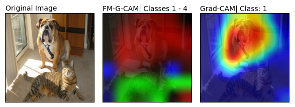
Figure 1: FM-G-CAM for general image classification tasks against Grad-CAM

In this paper, we propose a novel approach to produce a saliency map that could provide a unified approach to the visualisation of multiple class predictions; an example of the proposed approach can be observed in Figure 1. Our approach can be configured to consider any number of top classes to consider when generating the saliency map. The paper begins with a comparison of the existing methods to explain CNN predictions. Then, our new approach, FM-G-CAM and the theory behind it are explained mathematically and implemented as a Python package for public download. Following the theory, a list of practical use cases for which our approach could be effectively used is comparatively presented to the existing methods. Finally, the paper concludes with an in-depth discussion of how FM-G-CAM can be widely used to explain CNN predictions, drawbacks of it, and potential avenues to further improve it. The main scientific contributions of this work are as follows:

• A concise review of the existing saliency map generation techniques. Similarities, differences and drawbacks of them are discussed in the review, highlighting the gaps that exist. We explain the main three techniques in explaining CNN prediction and investigate further into the Activation-based saliency map generation methods.

• A Holistic approach to explain CNN prediction with example practical use cases. Addressing one of the main drawbacks we highlighted in the review of the existing work, a novel technique, Fused Multi-class Gradient-weighted Activation Map (FM-G-CAM), is introduced. FM-G-CAM is capable of considering multiple predictor classes in generating saliency maps and thereby providing a holistic explanation to CNN-based model predictions. We also provide an exhaustive mathematical and algorithmic explanation for FM-G-CAM, discussing the main concepts behind the novel technique in-depth.

• A practical usage examples comparative to Grad-CAM, highlighting FM-G-CAM’s benefits. The examples cover general use cases and a potential use case for Medical AI in Chest X-ray diagnosis. We used open-source, state-of-the-art models and datasets for the prediction tasks.

• A Python package for convenient generation of saliency maps for CNN predictions. We released this Pytorch-oriented library to the Python Package Index (PyPI), allowing the research community to use FM-G-CAM freely and conveniently via a Python library. The library supports different configurations of FM-G-CAM as well as the original Grad-CAM. We plan to maintain and improve this library to serve as a universal inferencing library that is focused on the Explainability of the predictions.

2 Existing Work

In this section, we critically evaluate the existing techniques to generate saliency maps for CNN-based predictions. We begin our discussion by discussing different methods of explaining the convolutions that happen in a CNN-based model. Then we summarise virtually all published CAM-based techniques, allowing the reader to clearly see the differences among each. Finally, we conclude the review of existing work by discussing the characteristics that make up a good saliency map.

2.1 Explaining Convolutions

Convolutions Neural Networks were long considered a black box [14] mainly due to the inability to logically explain CNN predictions. Currently, several methods exist to attempt to visually explain the inner workings of a CNN-based model, including CNN-based transformer models [15, 16, 17]. These visualisation methods predominantly use model properties such as, filter weights[18, 19], hidden neurons[20, 21, 22], and inference values which are discussed in the next section.

2.1.1 Inference values

Inference values of a CNN represent the inner workings of the model. These values include neuron activations, calculated gradients, main input, and main output. However, it is not very straightforward to visualise these values in a sensible way. To date, three main techniques have been used to meaningfully convert these quantitative values into a qualitative saliency map. Table 1 presents existing studies classified according to their techniques and drawbacks.

Table 1: Main techniques of CNN prediction visualisation

Technique	Studies
Perturbation	Blinded grey patches were used by Zeiler et al [23] to identify the areas of the image that have been affecting the prediction results. The variation of the targeted class score is recorded and then used to generate a saliency map visualising the areas that are important for the prediction. Later, this technique was further advanced, replacing the grey square with different pixel value alteration techniques like masking[24]. Although this technique is relatively straightforward, it is very inefficient since each altered patch has to be evaluated by inferencing the patched image through the model. The technique becomes even more inefficient when there is more than one patched/altered area in the image.
Propagation	This technique only requires the image to be propagated once forward and once backwards [25]. The bare gradients calculated while inferencing is used to generate the saliency map. This technique was much faster than pertubation-based techniques. However, the generated saliency maps were occasionally very noisy. Later, more studies were published addressing this noise issue by adding slight modifications to the back-propagation algorithm [26, 27, 28, 29]. The main drawback of this technique is the noisiness of the saliency maps.
Activation	Saliency maps generated using activations of the models while inferencing is commonly called a Class Activation Map (CAM). This was first introduced by Zhou et at. [30] using the activations of the feature maps at the penultimate layer. This was done by identifying the relevance of the activations to the final fully connected output related to the target class. However, this was only possible when the penultimate layer is a Global Average Pooling layer, which was the case back then for most of the typical CNN architectures. Later, Selvaraju et al. [10] presented a way to generate a saliency map with any CNN-based model by getting the CAM of the last convolutional layer and weigting them with the average of their gradients. This is currently the most popular method for generating saliency maps. Grad-CAM was further advanced by using also the second-order derivative in Grad-CAM++ [11]. The idea of Gradient-weighted Activations then created a series of techniques presented in the section 2.2. Lower resolution of the saliency map is one of the main drawbacks of this technique.

2.2 CAM-based techniques in summary

Class activations have shown prominent results in explaining CNN predictions mainly due to the information that CNN activations holds regarding the CNN’s decision making process in predictions. Table 2 presents a summary of the major CAM-based saliency map generation methods widely used.

Table 2: Common techniques for CNN prediction visualisation.

CAM Method	Brief
Grad-CAM [10]	Takes the activations of the last convolutional layer and weights them with the average gradients of the same layer with respect to the final fully connected output related to the target class
XGradCAM [31]	Follows a very similar technique to Grad-CAM in weighting activations. However, the calculated gradients were normalised prior to weighting.
HiResCAM [32]	No improvement is the the resolution of the CAM as the name suggests. However, instead of averaging the calculated gradients, in this study the authors multiply the activations element-wise by its corresponding gradient.
Seg-XRes-CAM [33]	A CAM method inspired by HiResCAM for generating saliency maps for segmentation maps, with a primary focus on object detection.
Ablation-CAM [34]	Generates the saliency map in a similar way to performing a ablation test. Sets the prediction activations to zero and measures the deviation in the prediction score. This measured deviation corresponding to the areas of the original image is then used to create the final saliency map.
Score-CAM [35]	Score-CAM removes the dependency on gradients for the generation of the saliency map using a two-stage approach. Instead of gradients, the importance of the activations is determined by a perturbation method similar to that of Ablation-CAM in the second stage.
Eigen-CAM [36]	Differently from most of the other CAM methods, Eigen-CAM uses the first principle component of the feature maps produced following a prediction. This technique can also generate a saliency map without a target class.
Layer-CAM [37]	Very similar to the Grad-CAM’s core techniques but can use an arbitrarily selected convolutional layer of the predictor CNN model.

In addition to the aforementioned methods, Collins et al. [38] propose a matrix factorisation-based method that segments the image intro areas based on prediction classes.

2.3 What makes up a good saliency map?

Investigating the existing literature, we identified four main areas that could potentially define the quality of a saliency map; activation weighting technique, colourmap type, resolution, and multiclass support.

The activation weighting technique affects the accuracy of the saliency map at the very fundamental level. It matters mainly because it is not only the activation that represents the "thinking" process of the CNN, but also the gradients that correspond to them. However, these gradients can be noisy and could cause unrelated activations to be boosted up in the weighting process [9].

Lui et al. [39] present a detailed analysis of different types of quantified colour maps used for data visualisation. Current CAM methods generally use ’viridis’ or ’jet’ colour maps in presenting the saliency map. Our opinion is that the ’viridis’ colourmap is more appropriate than ’jet’ for saliency maps since multiple colours included in the ’jet’ map can make the map more confusing. Colourmap ’viridis’ is also more suitable since we do not need to represent a narrower ranges for intensity in the map.

Generally, the resolution is low in saliency maps and will depend on the properties of the predictor model. If the predictor model has larger kernels the resulting saliency maps will also have larger resolution. However, the kernels tend to become smaller going deeper into the model. Morbidelli et al. [40] present a way to use image augmentation techniques to increase the resolution of the saliency map while having smaller activation maps. This is useful for classification problems with relatively smaller visual targets.

Lastly, we argue that the saliency map must consider multiple classes if and when available. Most of the CAM methods focus only on one targeted class and do not represent the whole context of the CNN model’s thinking process. As an attempt to address this issue, we introduce FM-G-CAM in this work.

3 Method

The Fused Multi-class Gradient-weighted Class Activation Map (FM-G-CAM) introduced in this study investigates the reasoning behind the model prediction in a broader way compared to the existing methods, thereby aiming to increase explainability. This section begins with a brief discussion of the background that led to the development of FM-G-CAM. Then, the proposed FM-G-CAM algorithm is presented and described.

According to the relevant literature, there is a knowledge gap in XAI for computer vision predictions where more than one class is possible for an input image. Although techniques such as Deep Feature Factorisation [38] work towards this problem, these approaches focus moreso on dissecting an area classified as a single class into multiple classes. The proposed FM-G-CAM approach aims to provide a more holistic explanation of a CNN prediction without relying on one class.

3.1 Theory

Building on the basic concepts of the Grad-CAM approach[10], FM-G-CAM targets multiple classes instead of a single class which affect the final prediction results. Grad-CAM focuses on a single output at a time, leaving out important information, especially in the case of multi-class classification. FM-G-CAM attempts to overcome this drawback by producing a multicoloured saliency map which highlights the spatial areas of the image corresponding to the top ($N^{*}$) predictions. This can be arbitrarily selected; in this study, the top 3 classes ($K=3$) are selected.

Here ($N=\left\{Prediction\ class\ numbers\right\}$), ($n\in N$) and ($N^{*}$) is defined as below:

$$N^{*}=\{n_{k}^{*}:\ \ n_{k}^{*}\in N,\ P\left(n_{1}^{*}\right)>\ldots>P\left(n_{K}^{*}\right)\ and\ k\mathbb{\in N,\ }1\leq k\leq K\}.$$ (1)

($P(n)$) denotes the predicted probability of the n^th class. For example, ($n_{1}^{*}$) represents the class number of the most probable predicted class. ($y^{n}$) represents the output of the final layer related to the n^th class:

$$\alpha_{c}^{n_{k}^{*}}=\ \frac{1}{I\times J}\sum_{i=1}^{I}{\sum_{j=1}^{J}{\ \frac{\partial y^{n_{k}^{*}}}{\partial a_{i,j}^{n_{k}^{*}}}}},\ where\ a^{n_{k}^{*}}\in\ \mathbb{R}^{I\times J}.$$ (2)

In equation 2, ($\alpha_{c}^{n_{k}^{*}}$) represents the importance matrix with respect to the class ($n_{k}^{*}$) and feature channel ($c$) while ($a$) represents the activated outputs of the convolutions. This will then be weighted based on their corresponding activations:

$$R^{n_{k}^{*}}=\frac{1}{C}\sum_{c=1}^{C}{\alpha_{c}^{n_{k}^{*}}a^{c},}\ where\ R^{n_{k}^{*}}\in\ \mathbb{R}^{I\times J}.$$ (3)

In equation 3, ($R^{n_{k}^{*}}$) represents the unfiltered saliency map related to the class ($n_{k}^{*}$) while ($N$) represents the number of classes.

The matrix ($S^{n_{k}^{*}}$) represent filtered saliency map sized ($I\times J$) related to the class ($n_{k}^{*}$). Each element ($S_{i,j}^{n_{k}^{*}}$) is defined as follows:

$$S_{i,j}^{n_{k}^{*}}=\left\{\begin{aligned} R_{i,j}^{n_{k}^{*}},\ \ &R_{i,j}^{n_{k}^{*}}=max(R_{i,j}^{n_{1}^{*}},\ldots,R_{i,j}^{n_{K}^{*}})\\ 0,\ \ &R_{i,j}^{n_{k}^{*}}\neq max(R_{i,j}^{n_{1}^{*}},\ldots,R_{i,j}^{n_{K}^{*}})\end{aligned}\right.\ ,\ \ where\ S^{n_{k}^{*}}\in\ \mathbb{R}^{I\times J}.$$ (4)

As mathematically shown in the above equation 4, the filtered saliency map only contains the highest value across the selected ($K$) classes for each element in a 2D matrix ($S^{n_{k}^{*}}$). Other elements are set to zero.

Then, differently from Grad-CAM, L2-normalisation is performed on a concatenated K-dimensional matrix ($S^{{}^{\prime}}$):

$$S^{{}^{\prime}}=\ \begin{bmatrix}S^{n_{1}^{*}}&\ldots&S^{n_{K}^{*}}\end{bmatrix},\ \ where\ S^{{}^{\prime}}\in\ \mathbb{R}^{I\times J\times K},$$ (5)

and passed into the ReLU activation function to get the final saliency map matrix ($S_{FM-G-CAM}$):

$$S_{FM-G-CAM}=ReLU\left(\frac{S^{{}^{\prime}}}{\left\|S^{{}^{\prime}}\right\|_{2}}\right).$$ (6)

As mentioned, ($K$) is set to 3 in this paper for ease of explanation. Deciding a value for ($K$) is discussed in section 3.3.

The L2-normalisation helps to normalise the feature maps across the classes, making the lower activations more pronounced and visible when visually displayed. A comprehensive visual demonstration and comparison between Grad-CAM and FM-G-CAM is done in section 5.

3.2 Algorithm

In this section, we present the algorithm that realises the mathematical equations explained in Section 3.1. This can be used as a guide when implementing this technique from scratch. Figure 2 visually shows the step-by-step generation of FM-G-CAM from the generation of Gradient-weighted activation maps to the final FM-G-CAM saliency map.

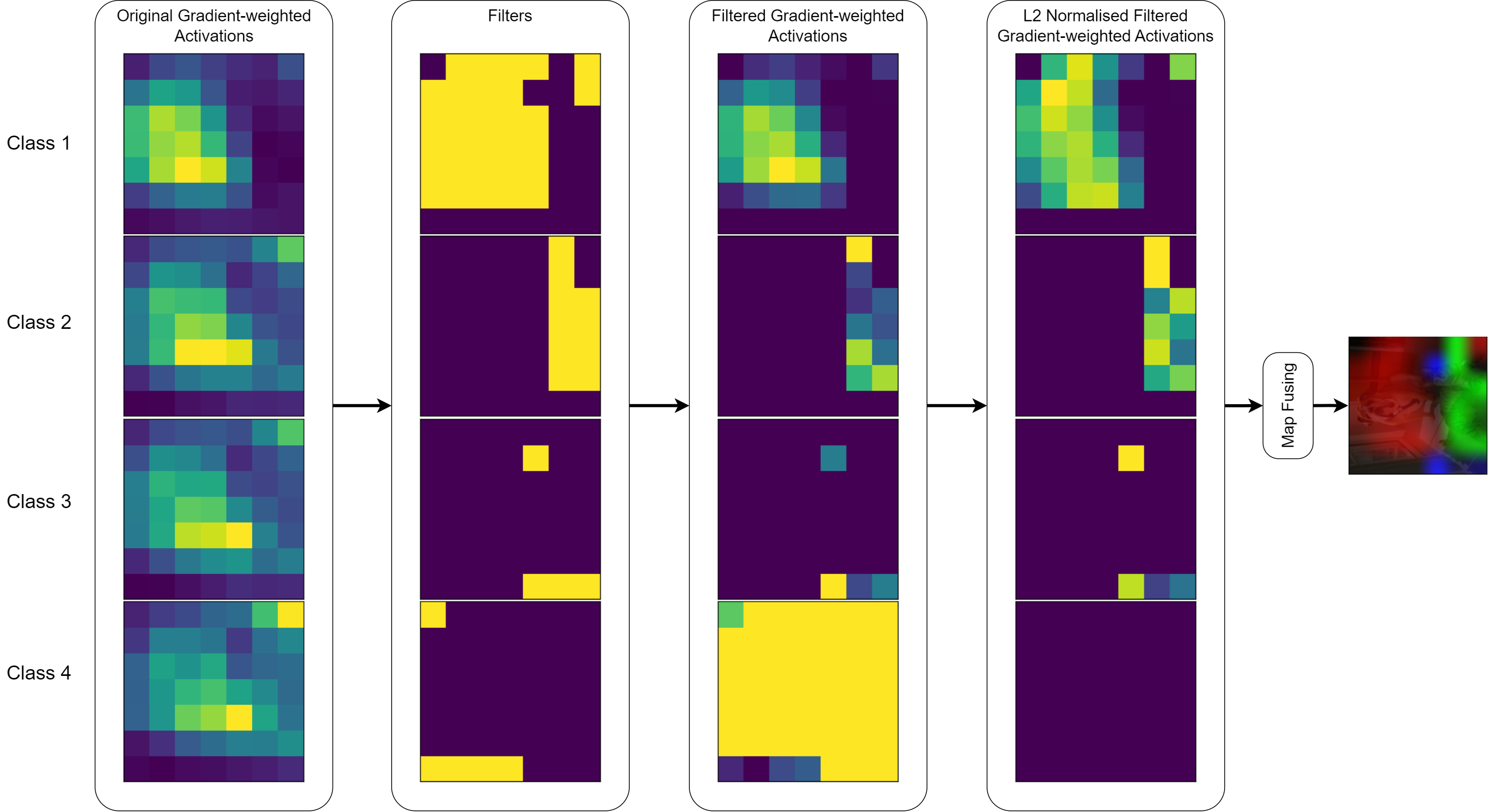
Figure 2: The process of generating FM-G-CAM.

Algorithm 1 Algorithm for generating FM-G-CAM

$n\geq 1$

$c\geq n$

$y\leftarrow 1$

$C\leftarrow c$

$N\leftarrow n$

$M=[]$

while $N\leq C$ do $\triangleright$ Calculation of Gradient-weighted Activation for each class

     $A_{C}\leftarrow$ Activations based on class $C$

     $W_{C}\leftarrow$ Gradients of the the activations of class $C$ w.r.t to the selected convolutional layer

     $M_{C}\leftarrow A_{C}*W_{C}$

     Append $M_{C}$ to $M$

end while

Filtering $\triangleright$ see section 3.1

Normalise $M$ $\triangleright$ L2 Norm

3.3 Choosing an optimal value for (K)

Unlike other saliency map generation methods, FM-G-CAM utilises multiple classes to generate the final saliency map. We recommend choosing the top predicted classes to be used. The top 3 or top 5 classes are recommended to be used with FM-G-CAM even though the algorithm allows any number of arbitrarily chosen classes to be used in the saliency map generation. However, this can be different and will depend mainly based below three factors: 1) The nature of the use case, 2) Average area of interest on the image for each predictive class, 3) Average number of distinct predictive labels per image.

Based on the above factors, an optimal number of classes to be used for the generation of saliency maps should be decided. Furthermore, these three factors reveal the complexity of the saliency map required to provide a holistic explanation of the model predictions.

3.3.1 Importance of L2 Normalisation

As shown in Figure 3, L2-Normalisation across the class gradient maps makes FM-G-CAM sensitive and unbiased, especially in the presence of classes with relatively lower weighted activations, while remaining accurate based on the content of the image. Also, as explained in the algorithm 1, normalisation is applied only after the filtering process. This allows filtering to be done based on raw gradient-weighted activations, and independent of the normalisation process. L2 normalisation also aids in the reduction of unwanted noise, as shown in figure 2. This is due to the fact that it is applied across the saliency maps by comparing the values against each other.

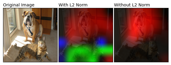
Figure 3: Effect of L2 Norm for saliency map generation in FM-G-CAM.

3.3.2 Choice of Colour Maps

Based on the findings presented in Section 2.3, we recommend using a single-colour colour map for each class when K in Section 3.3 is set to the recommended value of four. This will allow proper visualisation of the CNN’s decision-making process without overly complicating the saliency map. We comparatively test these in section 5 with existing methods.

4 Implementation: XAI Inference Engine

For convenient use of FM-G-CAM, a Python library is available to the community. The implementation is based on the algorithm 1. The code is open source and available on GitHub. The library allows the user to use their trained PyTorch CNN-based models with our library. The library will output the prediction results along with the generated FM-G-CAM saliency map explaining the results. Figure 4 shows the overview of the XAI Inference Engine.

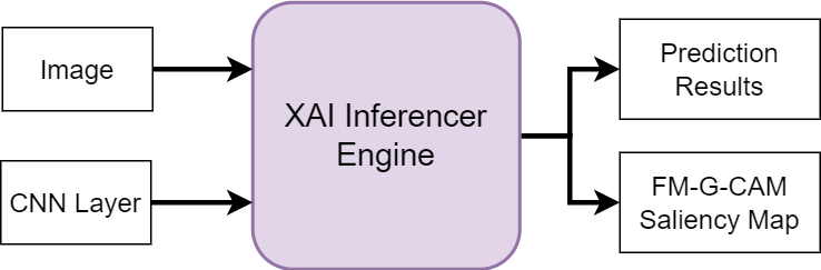
Figure 4: Overview of the XAI Inference Engine.

The library also allows changing the end activation function used in the saliency map generation to ReLU, ELU, or GeLU. Figure 5 shows the comparative results of the use of the different activation functions available. It shows that GeLU and ELU tend to attract more noise than ReLU. However, at the same time, those can be useful when we want the saliency maps to be more sensitive. In contrast, Grad-CAM remains identical across all activation functions.

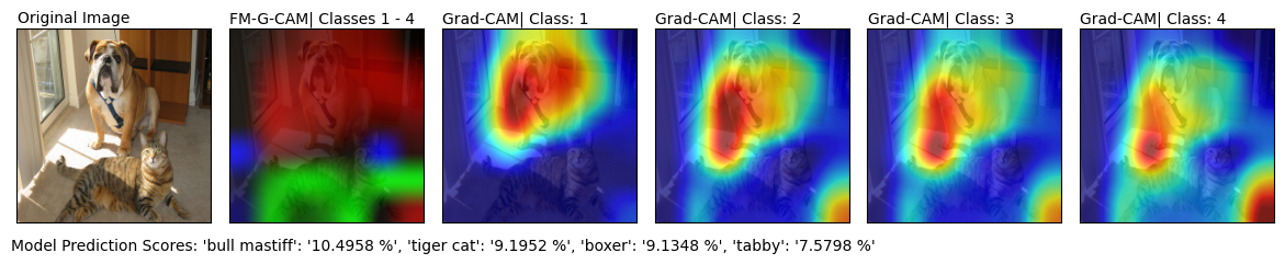
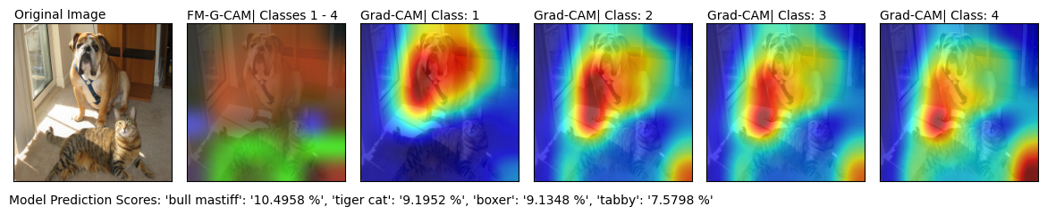
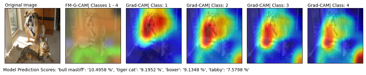
Figure 5: Overview of the XAI Inference Engine. Column 2 shows the output for FM-G-CAM, while columns 3 to 6 show the corresponding saliency map outputs from Grad-CAM.

5 Use cases: A Comparative Practical Guide for FM-G-CAM

In this section, we compare our method with the existing methods in generative saliency maps via a small subset of use cases. It is worth noting that the method we propose is characteristically different from virtually all of the existing methods due to the nature of considering multiple classes for the saliency map. To be as fair as possible, we perform Grad-CAM on all the classes that FM-G-CAM uses to generate the saliency map, as can be seen in the following sections. Also, we purposefully compare our technique only with Grad-CAM since any other improved or advanced version of Grad-CAM can be used within FM-G-CAM in the generation of the saliency map. We did not intend to improve the underlying theory of gradient-weighted activations for saliency map generation but to utilise that idea in a way to provide a more holistic explanation of CNN predictions. The following sections describe some example use cases of FM-G-CAM in comparison to Grad-CAM.

5.1 Image Classification

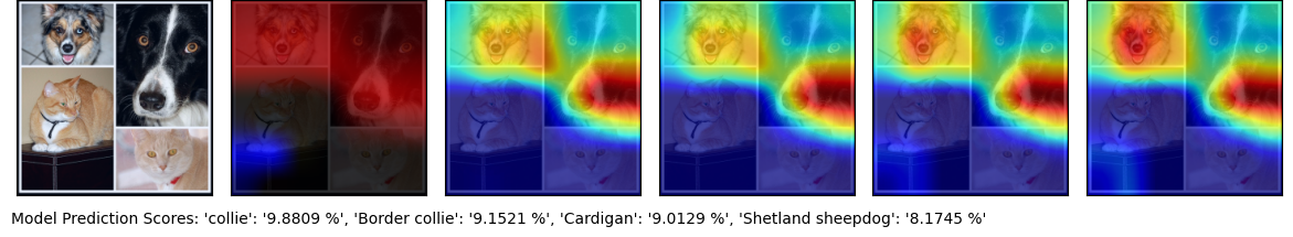
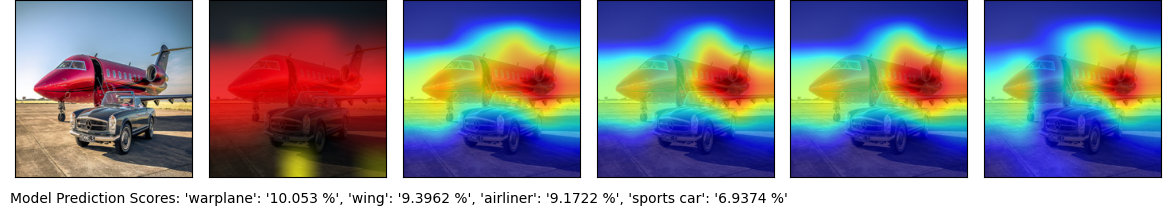
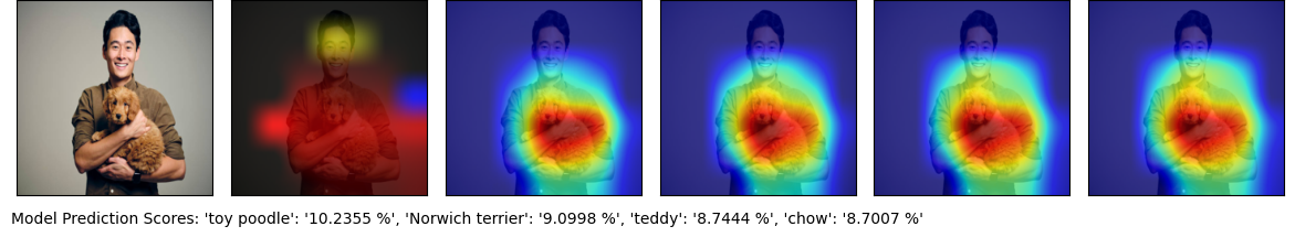
Figure 6: FM-G-CAM for general image classification tasks in comparison with Grad-CAM. Column 2 shows the output for FM-G-CAM, while columns 3 to 6 show the corresponding saliency map outputs from Grad-CAM.

Figure 6 shows some examples of using FM-G-CAM on random images. The predictor model used here is ResNet50V2 [41] with pre-trained ImageNet [13] weights available in the PyTorch model registry. The native preprocessing pipeline was used to preprocess the input image.

The prediction in the top row of figure 6 shows that even when Grad-CAM was generated for the top-4 classes, none of them clearly gives an indication of the existence of the ’tiger cat’ class. The proposed approach shows that there are two main classes that the model has focused on and then highlights the areas of them in the image. The intensity of the colour represents the importance of the highlighted area for the prediction. The prediction in the bottom row shows an interesting result since the model top-4 prediction list does not include a correct label for the human in the image. However, FM-G-CAM shows that there are two separate entities, while all four Grad-CAMs are similar.

5.2 Medical AI

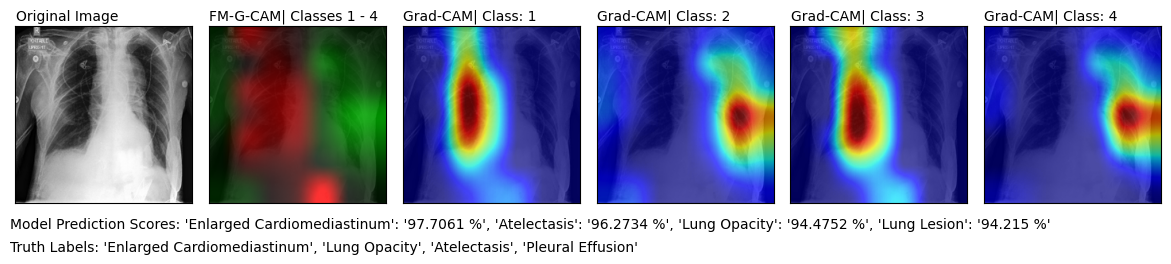
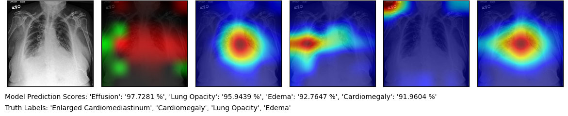
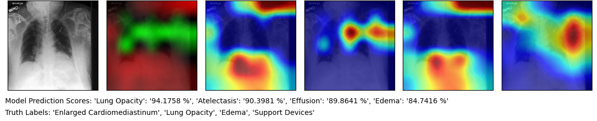
Figure 7: FM-G-CAM for general image classification tasks in comparison with Grad-CAM. Column 2 shows the output for FM-G-CAM, while columns 3 to 6 show the corresponding saliency map outputs from Grad-CAM.

Another very interesting and important area where the proposed approach can be utilised is in medical AI. According to the literature, CNNs are a popular approach in the field of medical AI for a variety of diagnosis modalities [42, 43, 44, 45]. Therefore, an application of FM-G-CAM is explored in the diagnosis of chest X-Ray images. To this end, TorchXRayVision[46] weights are used for the DenseNet model[47]. Figure 7 shows explained outputs when classifying images selected from the validation set. The samples show that the FM-G-CAM presents a holistic and singular saliency map that can replace all other class-based Grad-CAM saliency maps. Further, FM-G-CAM comparatively visualises the saliency maps of the selected classes, portraying their relative importance, whereas Grad-CAM considers each class in isolation, completely neglecting the fact that they are all part of the same prediction result.

6 Discussion

Using the CNN activations to explain their prediction was first introduced by [30], based on previous work investigating the capabilities of CNNs in object detection [48]. These works formed a basis for the idea of Grad-CAM [10]. However, these studies only consider a target class and, by doing so, disregard a considerable portion of information regarding the CNN classification process. This study proposes that the activations should be calculated for the top-k classes, weighing them accordingly using their gradients, normalising them for fair representation, and finally fusing them. Hence, while Grad-CAM and FM-G-CAM are based on the aforementioned studies, they are characteristically and mathematically different.

The previously discussed Figure 6 shows that the single-class Grad-CAM approach is not always useful in situations where a bigger-picture approach is needed. Instead, it only shows why a specified class has its related prediction score. In most cases, this class is selected as the top predicted class. However, there is a significant difference in the majority of CNN-based predictor models in top-1 accuracy vs top-5 accuracy. The difference between the accuracy of top-1 and the accuracy of top-5 can be substantial[41, 47]. Situations such as those arising from the interpretation of chest X-rays show that, in some cases, the top-k predictions where $k>1$ hold significantly useful information when interpreting the predictions.

7 Conclusion and Future Work

This work has highlighted the importance of using holistic visual explanations for CNN predictions. It is observed that most of the existing saliency map generation methods, such as Grad-CAM solely focus on a single target class, which can neglect important information related to the reasoning behind CNN’s prediction. While investigating the related literature, it was identified that the substantial differences observed in top-1 and top-5 predictions can cause saliency maps to lose relevance when focusing only on the most probable model output.

To overcome the identified gaps in the existing methodologies, this work introduced FM-G-CAM, an unbiased methodology that generates saliency maps capable of providing a comprehensive interpretation of the CNN model decision-making process. FM-G-CAM can be configured to consider multiple top classes in the saliency map generation, providing a more holistic visual explanation for CNN predictions. FM-G-CAM is presented using detailed mathematical and algorithmic explanations, along with a practical implementation guide. Further, to highlight FM-G-CAM’s capabilities, its effectiveness was compared with that of Grad-CAM via real-world use cases. All code for the approach is released under an open-source licence.

For future work, the proposed approach uses gradient-weighted activations, though there are other approaches such as Grad-CAM++[11]. Toward this, future work could utilise other methods to provide further comparison to the proposed FM-G-CAM approach. One limitation of this study is within the approach to increase the visibility of lower activations, which promotes unwanted noise in some cases. Therefore, future work could explore methods to eliminate unwanted noise while retaining the visibility of lower-weighted neuroneal activations.

Further analysis could also be performed, such as for the use cases of document analysis[49], climate predictions[50], and segmentation tasks[51, 52], to name a few. The possibility of using FM-G-CAM in object detection could also be investigated.

To finally conclude, this work proposes a form of explainable artificial intelligence and contributes to the ongoing discussion surrounding more holistic approaches to explainability in image classification problems.

References

- [1] Alejandro Barredo Arrieta, Natalia Díaz-Rodríguez, Javier Del Ser, Adrien Bennetot, Siham Tabik, Alberto Barbado, Salvador García, Sergio Gil-López, Daniel Molina, Richard Benjamins, et al. Explainable artificial intelligence (xai): Concepts, taxonomies, opportunities and challenges toward responsible ai. Information fusion, 58:82–115, 2020.
- [2] Dang Minh, H Xiang Wang, Y Fen Li, and Tan N Nguyen. Explainable artificial intelligence: a comprehensive review. Artificial Intelligence Review, pages 1–66, 2022.
- [3] Hui Wen Loh, Chui Ping Ooi, Silvia Seoni, Prabal Datta Barua, Filippo Molinari, and U Rajendra Acharya. Application of explainable artificial intelligence for healthcare: A systematic review of the last decade (2011–2022). Computer Methods and Programs in Biomedicine, page 107161, 2022.
- [4] Saad I Nafisah and Ghulam Muhammad. Tuberculosis detection in chest radiograph using convolutional neural network architecture and explainable artificial intelligence. Neural Computing and Applications, pages 1–21, 2022.
- [5] K Muthamil Sudar, P Nagaraj, S Nithisaa, R Aishwarya, M Aakash, and S Ishwarya Lakshmi. Alzheimer’s disease analysis using explainable artificial intelligence (xai). In 2022 International Conference on Sustainable Computing and Data Communication Systems (ICSCDS), pages 419–423. IEEE, 2022.
- [6] Laith Alzubaidi, Jinglan Zhang, Amjad J Humaidi, Ayad Al-Dujaili, Ye Duan, Omran Al-Shamma, José Santamaría, Mohammed A Fadhel, Muthana Al-Amidie, and Laith Farhan. Review of deep learning: Concepts, cnn architectures, challenges, applications, future directions. Journal of big Data, 8:1–74, 2021.
- [7] Kai Han, Yunhe Wang, Hanting Chen, Xinghao Chen, Jianyuan Guo, Zhenhua Liu, Yehui Tang, An Xiao, Chunjing Xu, Yixing Xu, et al. A survey on vision transformer. IEEE transactions on pattern analysis and machine intelligence, 45(1):87–110, 2022.
- [8] Salman Khan, Muzammal Naseer, Munawar Hayat, Syed Waqas Zamir, Fahad Shahbaz Khan, and Mubarak Shah. Transformers in vision: A survey. ACM computing surveys (CSUR), 54(10s):1–41, 2022.
- [9] Riccardo Guidotti, Anna Monreale, Salvatore Ruggieri, Franco Turini, Fosca Giannotti, and Dino Pedreschi. A survey of methods for explaining black box models. 51(5), aug 2018.
- [10] Ramprasaath R Selvaraju, Michael Cogswell, Abhishek Das, Ramakrishna Vedantam, Devi Parikh, and Dhruv Batra. Grad-cam: Visual explanations from deep networks via gradient-based localization. In Proceedings of the IEEE international conference on computer vision, pages 618–626, 2017.
- [11] Aditya Chattopadhay, Anirban Sarkar, Prantik Howlader, and Vineeth N Balasubramanian. Grad-cam++: Generalized gradient-based visual explanations for deep convolutional networks. In 2018 IEEE winter conference on applications of computer vision (WACV), pages 839–847. IEEE, 2018.
- [12] Jaya Gupta, Sunil Pathak, and Gireesh Kumar. Deep learning (cnn) and transfer learning: a review. In Journal of Physics: Conference Series, volume 2273, page 012029. IOP Publishing, 2022.
- [13] Jia Deng, Wei Dong, Richard Socher, Li-Jia Li, Kai Li, and Li Fei-Fei. Imagenet: A large-scale hierarchical image database. In 2009 IEEE conference on computer vision and pattern recognition, pages 248–255. Ieee, 2009.
- [14] Riccardo Guidotti, Anna Monreale, Salvatore Ruggieri, Franco Turini, Fosca Giannotti, and Dino Pedreschi. A survey of methods for explaining black box models. ACM Comput. Surv., 51(5), aug 2018.
- [15] Nebras Sobahi, Orhan Atila, Erkan Deniz, Abdulkadir Sengur, and U. Rajendra Acharya. Explainable covid-19 detection using fractal dimension and vision transformer with grad-cam on cough sounds. Biocybernetics and Biomedical Engineering, 42(3):1066–1080, 2022.
- [16] Hila Chefer, Shir Gur, and Lior Wolf. Transformer interpretability beyond attention visualization. In Proceedings of the IEEE/CVF Conference on Computer Vision and Pattern Recognition (CVPR), pages 782–791, June 2021.
- [17] Michal Jungiewicz, Piotr Jastrzebski, Piotr Wawryka, Karol Przystalski, Karol Sabatowski, and Stanisław Bartus. Vision transformer in stenosis detection of coronary arteries. Expert Systems with Applications, 228:120234, 2023.
- [18] Alex Krizhevsky, Ilya Sutskever, and Geoffrey E Hinton. Imagenet classification with deep convolutional neural networks. In F. Pereira, C.J. Burges, L. Bottou, and K.Q. Weinberger, editors, Advances in Neural Information Processing Systems, volume 25. Curran Associates, Inc., 2012.
- [19] Shuo Wang, Tonghai Wu, and Kunpeng Wang. Automated 3d ferrograph image analysis for similar particle identification with the knowledge-embedded double-cnn model. Wear, 476:203696, 2021. 23rd International Conference on Wear of Materials.
- [20] Paulo E. Rauber, Samuel G. Fadel, Alexandre X. Falcão, and Alexandru C. Telea. Visualizing the hidden activity of artificial neural networks. IEEE Transactions on Visualization and Computer Graphics, 23(1):101–110, 2017.
- [21] Aravindh Mahendran and Andrea Vedaldi. Visualizing deep convolutional neural networks using natural pre-images. International Journal of Computer Vision, 120(3):233–255, 2016. Communicated by Cordelia Schmid.
- [22] David Bau, Bolei Zhou, Aditya Khosla, Aude Oliva, and Antonio Torralba. Network dissection: Quantifying interpretability of deep visual representations. In 2017 IEEE Conference on Computer Vision and Pattern Recognition (CVPR), pages 3319–3327, 2017.
- [23] Matthew D. Zeiler and Rob Fergus. Visualizing and understanding convolutional networks. In David Fleet, Tomas Pajdla, Bernt Schiele, and Tinne Tuytelaars, editors, Computer Vision – ECCV 2014, pages 818–833, Cham, 2014. Springer International Publishing.
- [24] Luisa M Zintgraf, Taco S Cohen, Tameem Adel, and Max Welling. Visualizing deep neural network decisions: Prediction difference analysis. arXiv e-prints, pages arXiv–1702, 2017.
- [25] K Simonyan, A Vedaldi, and A Zisserman. Deep inside convolutional networks: visualising image classification models and saliency maps. In Proceedings of the International Conference on Learning Representations (ICLR). ICLR, 2014.
- [26] J Springenberg, Alexey Dosovitskiy, Thomas Brox, and M Riedmiller. Striving for simplicity: The all convolutional net. In ICLR (workshop track), 2015.
- [27] Sebastian Bach, Alexander Binder, Gregoire Montavon, Frederick Klauschen, Klaus-Robert Muller, and Wojciech Samek. On pixel-wise explanations for non-linear classifier decisions by layer-wise relevance propagation. PloS one, 10(7):e0130140, 2015.
- [28] Mukund Sundararajan, Ankur Taly, and Qiqi Yan. Axiomatic attribution for deep networks. In International conference on machine learning, pages 3319–3328. PMLR, 2017.
- [29] Grégoire Montavon, Sebastian Lapuschkin, Alexander Binder, Wojciech Samek, and Klaus-Robert Müller. Explaining nonlinear classification decisions with deep taylor decomposition. Pattern recognition, 65:211–222, 2017.
- [30] Bolei Zhou, Aditya Khosla, Agata Lapedriza, Aude Oliva, and Antonio Torralba. Learning deep features for discriminative localization. In Proceedings of the IEEE conference on computer vision and pattern recognition, pages 2921–2929, 2016.
- [31] Ruigang Fu, Qingyong Hu, Xiaohu Dong, Yulan Guo, Yinghui Gao, and Biao Li. Axiom-based grad-cam: Towards accurate visualization and explanation of cnns. arXiv preprint arXiv:2008.02312, 2020.
- [32] Rachel Lea Draelos and Lawrence Carin. Use hirescam instead of grad-cam for faithful explanations of convolutional neural networks. arXiv preprint arXiv:2011.08891, 2020.
- [33] Syed Nouman Hasany, Caroline Petitjean, and Fabrice Mériaudeau. Seg-xres-cam: Explaining spatially local regions in image segmentation. In Proceedings of the IEEE/CVF Conference on Computer Vision and Pattern Recognition (CVPR) Workshops, pages 3733–3738, June 2023.
- [34] Saurabh Desai and Harish G. Ramaswamy. Ablation-cam: Visual explanations for deep convolutional network via gradient-free localization. In 2020 IEEE Winter Conference on Applications of Computer Vision (WACV), pages 972–980, 2020.
- [35] Haofan Wang, Zifan Wang, Mengnan Du, Fan Yang, Zijian Zhang, Sirui Ding, Piotr Mardziel, and Xia Hu. Score-cam: Score-weighted visual explanations for convolutional neural networks. In Proceedings of the IEEE/CVF conference on computer vision and pattern recognition workshops, pages 24–25, 2020.
- [36] Mohammed Bany Muhammad and Mohammed Yeasin. Eigen-cam: Class activation map using principal components. In 2020 international joint conference on neural networks (IJCNN), pages 1–7. IEEE, 2020.
- [37] Peng-Tao Jiang, Chang-Bin Zhang, Qibin Hou, Ming-Ming Cheng, and Yunchao Wei. Layercam: Exploring hierarchical class activation maps for localization. IEEE Transactions on Image Processing, 30:5875–5888, 2021.
- [38] Edo Collins, Radhakrishna Achanta, and Sabine Susstrunk. Deep feature factorization for concept discovery. In Proceedings of the European Conference on Computer Vision (ECCV), pages 336–352, 2018.
- [39] Yang Liu and Jeffrey Heer. Somewhere over the rainbow: An empirical assessment of quantitative colormaps. In Proceedings of the 2018 CHI Conference on Human Factors in Computing Systems, CHI ’18, page 1–12, New York, NY, USA, 2018. Association for Computing Machinery.
- [40] Pietro Morbidelli, Diego Carrera, Beatrice Rossi, Pasqualina Fragneto, and Giacomo Boracchi. Augmented grad-cam: Heat-maps super resolution through augmentation. In ICASSP 2020 - 2020 IEEE International Conference on Acoustics, Speech and Signal Processing (ICASSP), pages 4067–4071, 2020.
- [41] Kaiming He, Xiangyu Zhang, Shaoqing Ren, and Jian Sun. Identity mappings in deep residual networks. In Computer Vision–ECCV 2016: 14th European Conference, Amsterdam, The Netherlands, October 11–14, 2016, Proceedings, Part IV 14, pages 630–645. Springer, 2016.
- [42] DR Sarvamangala and Raghavendra V Kulkarni. Convolutional neural networks in medical image understanding: a survey. Evolutionary intelligence, 15(1):1–22, 2022.
- [43] Jeremy Irvin, Pranav Rajpurkar, Michael Ko, Yifan Yu, Silviana Ciurea-Ilcus, Chris Chute, Henrik Marklund, Behzad Haghgoo, Robyn Ball, Katie Shpanskaya, et al. Chexpert: A large chest radiograph dataset with uncertainty labels and expert comparison. In Proceedings of the AAAI conference on artificial intelligence, volume 33, pages 590–597, 2019.
- [44] Ahmad Waleed Salehi, Preety Baglat, Brij Bhushan Sharma, Gaurav Gupta, and Ankita Upadhya. A cnn model: earlier diagnosis and classification of alzheimer disease using mri. In 2020 International Conference on Smart Electronics and Communication (ICOSEC), pages 156–161. IEEE, 2020.
- [45] Woo Kyung Moon, Yan-Wei Lee, Hao-Hsiang Ke, Su Hyun Lee, Chiun-Sheng Huang, and Ruey-Feng Chang. Computer-aided diagnosis of breast ultrasound images using ensemble learning from convolutional neural networks. Computer methods and programs in biomedicine, 190:105361, 2020.
- [46] Joseph Paul Cohen, Joseph D Viviano, Paul Bertin, Paul Morrison, Parsa Torabian, Matteo Guarrera, Matthew P Lungren, Akshay Chaudhari, Rupert Brooks, Mohammad Hashir, et al. Torchxrayvision: A library of chest x-ray datasets and models. In International Conference on Medical Imaging with Deep Learning, pages 231–249. PMLR, 2022.
- [47] Gao Huang, Zhuang Liu, Laurens Van Der Maaten, and Kilian Q Weinberger. Densely connected convolutional networks. In Proceedings of the IEEE conference on computer vision and pattern recognition, pages 4700–4708, 2017.
- [48] Zhou Bolei, Aditya Khosla, Agata Lapedriza, Aude Oliva, and Antonio Torralba. Object detectors emerge in deep scene cnns. 2015.
- [49] Sai Chandra Kosaraju, Mohammed Masum, Nelson Zange Tsaku, Pritesh Patel, Tanju Bayramoglu, Girish Modgil, and Mingon Kang. Dot-net: Document layout classification using texture-based cnn. In 2019 International Conference on Document Analysis and Recognition (ICDAR), pages 1029–1034, 2019.
- [50] Ashesh Chattopadhyay, Pedram Hassanzadeh, and Saba Pasha. Predicting clustered weather patterns: A test case for applications of convolutional neural networks to spatio-temporal climate data. Scientific reports, 10(1):1317, 2020.
- [51] Konstantinos Kamnitsas, Christian Ledig, Virginia FJ Newcombe, Joanna P Simpson, Andrew D Kane, David K Menon, Daniel Rueckert, and Ben Glocker. Efficient multi-scale 3d cnn with fully connected crf for accurate brain lesion segmentation. Medical image analysis, 36:61–78, 2017.
- [52] Jose Dolz, Karthik Gopinath, Jing Yuan, Herve Lombaert, Christian Desrosiers, and Ismail Ben Ayed. Hyperdense-net: a hyper-densely connected cnn for multi-modal image segmentation. IEEE transactions on medical imaging, 38(5):1116–1126, 2018.