Spin fractionalization and zero modes in the spin-$\frac{1}{2}$ XXZ chain with boundary fields

Abstract

In this work we argue that the antiferromagnetic spin $\frac{1}{2}$ XXZ chain in the gapped phase with boundary magnetic fields hosts fractional spin $\frac{1}{4}$ at its edges. Using a combination of Bethe ansatz and the density matrix renormalization group we show that these fractional spins are sharp quantum observables in both the ground and the first excited state as the associated fractional spin operators have zero variance. In the limit of zero edge fields, we argue that these fractional spin operators once projected onto the low energy subspace spanned by the ground state and the first excited state, identify with the strong zero energy mode discovered by P. Fendley Fendley (2016).

I Introduction

Since the discovery of solitons carrying half of the electron charge Jackiw and Rebbi (1976); Su et al. (1979) it has been widely recognized Goldstone and Wilczek (1981); Kivelson and Schriefer (1982); Jackiw et al. (1983) that some states of matter can be characterized by fractional quantum numbers. Maybe the most celebrated example is the fractional quantum Hall state where quasiparticles carry fractional charges Laughlin (1983); Tsui et al. (1982). Other prominent examples coming from topological phases with short range topological order, such as symmetry protected topological (SPT) systems in one dimension, include spin-$1/2$ edge states in the spin one Haldane chain Haldane (1983); Affleck et al. (1987) as well as spin-$1/4$ zero energy modes (ZEM) localized at the edges of one dimensional spin triplet superconductors Keselman and Berg (2015); Pasnoori et al. (2020, 2021). In higher dimensions, surface states in topological insulators as well as disordered magnetic systems like spin ice Castelnovo et al. (2012) and spin liquids also exhibits signatures of fractionalization Banerjee et al. (2016).

In this work we shall demonstrate that fractionalization can also occur in more conventional magnetic systems which exhibit long range magnetic order. To this end we shall consider the paradigmatic XXZ spin $1/2$ chain with magnetic fields at its two edges, that we solve exactly with the Bethe ansatz and numerically using the density matrix renormalization group (DMRG), and show that in the low energy sector it hosts quantum spin-$1/4$ states localized at the edges. We shall further argue that this fractional quarter spins are sharp quantum observables. We believe that this result might have some impact in understanding dynamics Liu and Andrei (2014); Lancaster and Mitra (2010); Pozsgay et al. (2014); Mestyán et al. (2015); Foster et al. (2011); Joel et al. (2013); Misguich et al. (2017), heat and spin transport Bertini et al. (2016); De Luca et al. (2017); Bulchandani et al. (2018).

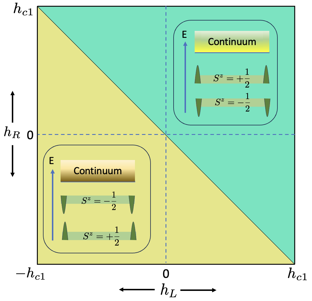
Figure 1: Ground state phase diagram of the XXZ model with edge fields smaller than the critical field $|h_{L,R}|<h_{c}=\Delta-1$ and for an odd number of sites. In each of the two phases separated by the line $h_{L}+h_{R}=0$ we show the ground state as well as the first excited state which is a midgap state below the continuum. Both states host fractional quarter spins ${\cal S}_{L,R}=\pm 1/4$ at both edges of the chain. These fractional spins are sharp quantum observables which reconstruct the total spin of each state $S^{z}={\cal S}_{L}+{\cal S}_{R}=\pm 1/2$. The $\pm 1/4$ quarter spins are depicted by triangles pointing upward and downward respectively. On the separatrix $h_{L}+h_{R}=0$ there is spontaneous symmetry breaking and the edge spin operator becomes a zero energy mode.

We consider the XXZ hamiltonian with boundary magnetic fields $(h_{L},h_{R})$ at the left and the right edges of an open chain

$$H = \sum_{j=1}^{N-1}\sigma^{x}_{j}\sigma^{x}_{j+1}+\sigma^{y}_{j}\sigma^{y}_{j+1}+\Delta(\sigma^{z}_{j}\sigma^{z}_{j+1}-1)$$ (1)

$$+ h_{L}\sigma^{z}_{1}+h_{R}\sigma^{z}_{N}$$

where $\sigma_{j}^{x,y,z}$ are the Pauli matrices and $\Delta>1$ is the anisotropy parameter. In the limit where the boundary fields are zero, on top of being $U(1)$ symmetric, (1) is space parity $\mathbb{P}$ and time reversal $\mathbb{T}$ invariant. It is also invariant under the $\mathbb{Z}_{2}=\{1,\tau\}$ spin flip symmetry, i.e: $[H,\tau]=0$ where $\tau=\Pi_{1}^{N}\sigma_{j}^{x}$. For generic non zero boundary fields $h_{L,R},\neq 0$, both $\mathbb{P}$ and $\mathbb{Z}_{2}$ symmetries are explicitly broken. However, on the two lines $h_{L}=\pm h_{R}$ the hamiltonian (1) displays $\mathbb{P}$ and $\mathbb{P}\circ\mathbb{Z}_{2}$ symmetries respectively.

The Hamiltonian in Eq. (1) is integrable by the method of the Bethe ansatz for arbitrary boundary fields $h_{L,R}$ and $\Delta$, which is used in the present paper to determine the low energy eigenstates analytically. The system with periodic boundary conditions was first solved by Bethe Bethe (1931) in the isotropic limit, $\Delta\rightarrow 1$. The solution was later extended to include anisotropy along the z-direction Orbach (1958); Walker (1959); Yang and Yang (1966a, b, c); Babelon et al. (1983). In the gapped regime ($\Delta>1$) it exhibits a continuous $U(1)$ symmetry and also a discrete $\mathbb{Z}_{2}$ spin flip symmetry. The discrete $\mathbb{Z}_{2}$ symmetry is spontaneously broken Syljuåsen (2003) and in the thermodynamic limit the system exhibits two degenerate symmetry broken ground states Takahashi (1999). The Bethe ansatz method to include the boundaries was developed in Alcaraz et al. (1987); Cherednik (1984); Sklyanin (1988) and the ground state and boundary excitations in various bulk phases exhibited by the XXZ spin chain were found in Skorik and Saleur (1995); S.Skorik and A.Kapustin (1995); Grijalva et al. (2019); Nassar and Tirkkonen (1998). An independent method to diagonalize the Hamiltonian using vertex operators was developed in Davies et al. (1993); Jimbo et al. (1992), and was later extended to include the boundary fields in Jimbo et al. (1995) where the boundary S-matrix and the integral formula for correlation functions have been found. Recently new band structures in the spectrum at large anisotropies have been found Sharma and Haque (2014).

Numerically we solve the model using DMRG, implemented through the TeNPy software Hauschild and Pollmann (2018), that allows access to the ground state and midgap state with arbitrary precision thanks to the gapped nature of both of these states. We take a maximum bond dimension of 400, with a minimal singular value decomposition cut off of $10^{-10}$, and converge the energy up to a maximal energy error on the order of $\sim 10^{-10}$.

When $\Delta>1$ the ground state $|g\rangle$ displays antiferromagnetic order with non zero staggered magnetization $\sigma=\lim_{N\rightarrow\infty}N^{-1}\sum_{j=1}^{N}(-1)^{j}\langle g|\sigma_{j}^{z}|g\rangle$ and is gapped. Indeed, for all values of the edge fields, there is a gap ($m$) in the spectrum to single particle spin $1/2$ spinon excitations

$$m=\sinh\gamma\sum_{n\in\mathbb{Z}}\frac{(-1)^{n}}{\cosh\gamma n},\;\Delta=\cosh{\gamma}.$$ (2)

However at low fields, i.e: $|h_{L,R}|<\Delta-1$, the lowest excited state is a midgap state $|e\rangle$ which lies below the continuum. We obtain the bound state energies which are given by

$$m_{\alpha}=h_{\alpha}+\sinh\gamma\sum_{n\in\mathbb{Z}}(-1)^{n}\;\frac{\sinh(\gamma{\epsilon}_{\alpha}|n|)}{\cosh\gamma n}e^{-\gamma|n|}$$ (3)

where $\alpha=(L,R)$. This midgap state is reminiscent of the existence of spin $1/2$ boundary bound states, localized at the two left and right edges. The spin quantum numbers and energies of the ground state as well as the midgap state depend on both the parity of the number of sites, $(-1)^{N}$, as well as on the boundary fields $h_{L,R}$. When $N$ is odd, the two states $|g\rangle$ and $|e\rangle$ have opposite total spins $S^{z}=\pm 1/2$. Taking as a reference state the $|-\frac{1}{2}\rangle$ state with energy $E_{0}$, the $|+\frac{1}{2}\rangle$ state is obtained by adding a localized bound state at each edge. This state has energy $E_{0}+m_{L}+m_{R}$. Depending on the edge magnetic fields, and hence on the sign of $m_{L}+m_{R}$, the ground state and the midgap state ($|g\rangle$,$|e\rangle$) are ($|-\frac{1}{2}\rangle,|+\frac{1}{2}\rangle$) when $h_{L}+h_{R}>0$ and ($|\frac{1}{2}\rangle,|-\frac{1}{2}\rangle$) when $h_{L}+h_{R}<0$. Notice that on the line $h_{L}+h_{R}=0$, the two states $|\pm\frac{1}{2}\rangle$ are degenerate. In the $N\rightarrow\infty$ limit, there is spontaneous symmetry breaking (SSB) of the $\mathbb{P}\circ\mathbb{Z}_{2}$ symmetry. In the particular case of zero edge fields, both $\mathbb{P}$ and $\mathbb{Z}_{2}$ symmetries are spontaneously broken. For $N$ even both ($|g\rangle$,$|e\rangle$) states have total spins $S^{z}=0$ and the bound state construction is presented in the Appendix. We display in Fig.(1) the phase diagram for low fields for an odd number of sites $N$.

II Spin Profiles

Due to the open boundaries and the presence of the edge fields $(h_{L},h_{R})$, the spin profiles $S^{z}_{j}=\langle\sigma_{j}^{z}\rangle/2$ in both the ground state and the midgap state differ from the bulk antiferromagnetic order close to the boundaries. For large enough $N$ we may write

$$S^{z}_{j}=(-1)^{j}\frac{\sigma}{2}+\Delta S^{z}(j),$$ (4)

where

$$\sigma=\pm\left(\Pi_{n=1}^{\infty}(\frac{1-q^{2n}}{1+q^{2n}})\right)^{2},\;q=e^{-\gamma},$$ (5)

is the exact staggered magnetization of the XXZ chain in the thermodynamical limit and $\Delta S^{z}(j)$ is the relative deviation with respect to the AF bulk profile. Due to the gap in the bulk these deviations are expected to be localized close to both the left and the right edges

$$\Delta S^{z}(j)=\Delta S^{z}_{L}(j)+\Delta S^{z}_{R}(j),$$ (6)

where $\Delta S^{z}_{L,R}(j)$ are localized close to $j=1$ and $j=N$ respectively (i.e: $\Delta S^{z}_{L,R}({N/2})\sim e^{-N/2}$). This is indeed what we find. We plot in Fig. 2 our DMRG results for $\Delta S^{z}_{L}(j)$ in both the ground state and the midgap state. We clearly observe an exponential localization of the relative spin accumulation for various values of $\Delta$ at constant boundary fields $h_{L}=h_{R}=0.2$ (see insets of Fig. 2).

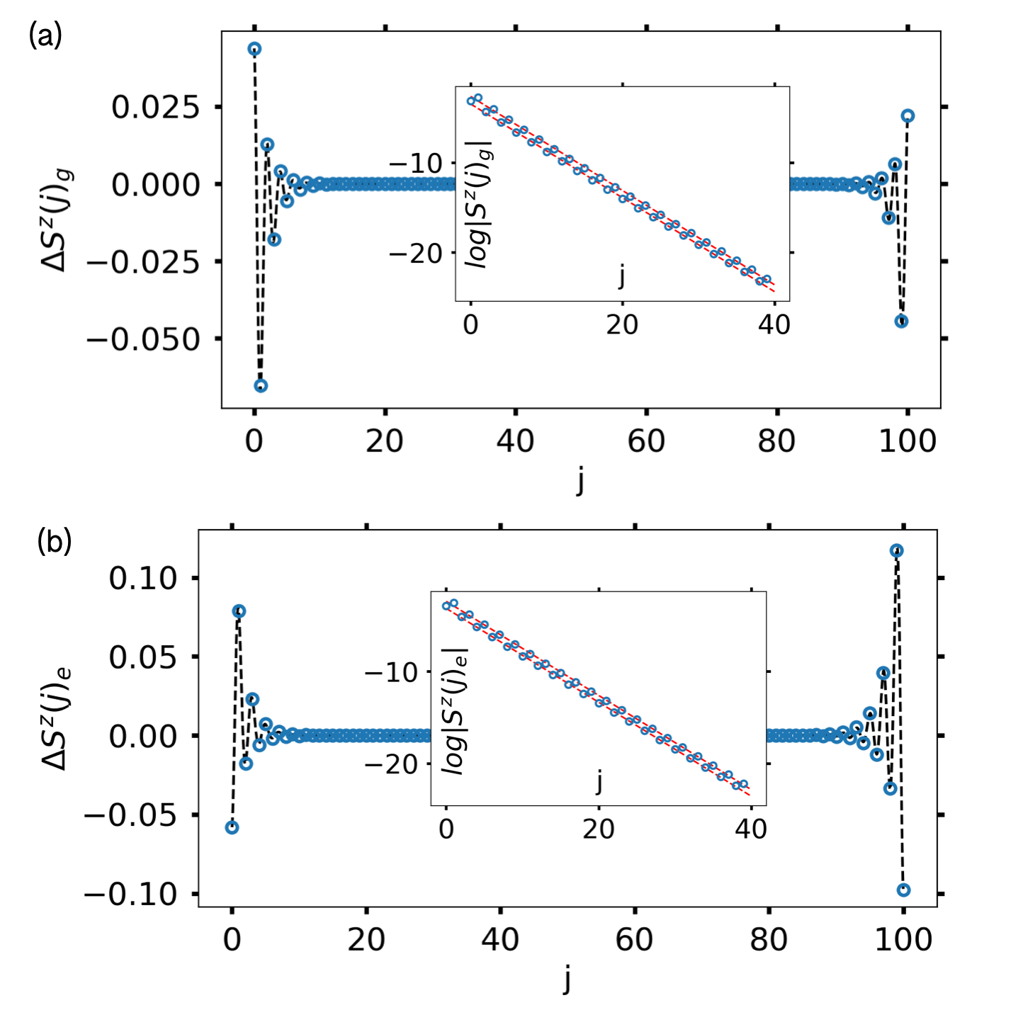
Figure 2: Spin profile $\Delta S^{z}(j)$ and the fitting of ansatz (a) in the ground state $|g\rangle$ with total spin $S^{z}=-\frac{1}{2}$ (b) in the midgap state $|e\rangle$ with total spin $S^{z}=\frac{1}{2}$ for model parameters $N=101$, $h_{L}=0.1,h_{R}=0.5$ and $\Delta=3$. The insets show that the relative spin are indeed localized exponentially on the edge, with red dashed lines representing excellent linear fits on the log-scale.

III Spin fractionalization

The above spin accumulations, or depletion, do not come as a surprise and are expected due to the open boundaries and the presence of the edge fields. What is non trivial is that they correspond to a genuine spin fractionalization in both the ground state and the midgap state. As we shall now demonstrate, in the thermodynamical limit and for all $\Delta>1,h_{{L},{R}}$, there exist fractionalized quarter spin operators associated with each edge, ${\cal\hat{S}}^{z}_{L}$ and ${\cal\hat{S}}^{z}_{R}$, which have well defined fractional eigenvalues

$${\cal\hat{S}}^{z}_{{L},{R}}|g(e)\rangle={\cal S}_{{L},{R}}|g(e)\rangle,\;{\cal S}^{z}_{L,R}=\pm\frac{1}{4}.$$ (7)

In the basis $(|g\rangle,|e\rangle)$ the above fractional spin operators commute with each other, and anticommute with the spin flip operator, i.e: $[{\cal\hat{S}}^{z}_{L},{\hat{S}}^{z}_{R}]=0$, $\{\tau,{\cal\hat{S}}^{z}_{L,R}\}=0$. Together, they reconstruct the z-component of the total spin $\hat{S}^{z}=\sum_{i=1}^{N}\hat{S}_{i}^{z}$, namely

$$\hat{S}^{z}={\cal\hat{S}}^{z}_{L}+{\cal{\hat{S}}}^{z}_{R}.$$ (8)

Since the edge spin operators have fractional spin $\pm 1/4$ one may verify that the $\hat{S}^{z}$ have eigenvalues $0$ or $\pm 1/2$ depending on whether $N$ is even or odd. For the fractional spin operators (7) to describe sharp quantum observables in the subspace spanned by $(|g\rangle,|e\rangle)$, not only they have to average to $\pm 1/4$ in both states, but also their variance must vanish in the thermodynamical limit, i.e:

$$\langle{\hat{S}}^{z}_{{L},{R}}\rangle = {\cal S}_{{L},{R}},$$ (9)

and

$$\delta{\cal S}^{2}_{{L},{R}} {\color[rgb]{0,0,1}\equiv} \langle({\cal\hat{S}}^{z}_{{L},{R}})^{2}\rangle-({\cal S}_{{L},{R}})^{2}=0,$$ (10)

where the average $\langle...\rangle$ is taken in each of the two states $(|g\rangle$ and $|e\rangle)$.

Following the authors of Refs.Kivelson and Schriefer (1982); Jackiw et al. (1983) we define the fractional spin operators as their convolution with a decaying function $f(x)$, here we take $f(x)=e^{-\alpha x}$ to write

$${\cal\hat{S}}^{z}_{L} = \lim_{\alpha\rightarrow 0}\lim_{N\rightarrow\infty}\sum_{j=1}^{N}f(j)\frac{\sigma^{z}_{j}}{2},$$ (11)

$${\cal\hat{S}}^{z}_{R} = \lim_{\alpha\rightarrow 0}\lim_{N\rightarrow\infty}\sum_{j=1}^{N}f(N+1-j)\frac{\sigma^{z}_{j}}{2},$$ (12)

which takes the limit $\alpha\rightarrow 0$ after the limit $N\rightarrow\infty$. We stress that the order of limits in (12) is important since by taking the limit $\alpha\rightarrow 0$ first, both ${\cal S}^{z}_{{L},{R}}$ would identify with the total magnetization $S^{z}$.

Due to the AF long range order it is convenient to distinguish between the contributions of the staggered part of the spin profile and that of the exponentially localized contributions

$${\cal\hat{S}}^{z}_{{L}}=-\frac{\sigma}{4}+{\Delta\cal\hat{S}}^{z}_{{L}},\;{\cal\hat{S}}^{z}_{{R}}=-\frac{\sigma}{4}(-1)^{N}+{\Delta\cal\hat{S}}^{z}_{{R}}.$$ (13)

where the relative accumulation operators are given by

$${\Delta\cal\hat{S}}^{z}_{{L}} = \lim_{\alpha\rightarrow 0}\lim_{N\rightarrow\infty}\frac{1}{2}\sum_{j=1}^{N}[\sigma_{j}^{z}-\sigma(-1)^{j}]e^{-\alpha j},$$

$${\Delta\cal\hat{S}}^{z}_{{R}} = \lim_{\alpha\rightarrow 0}\lim_{N\rightarrow\infty}\frac{1}{2}\sum_{j=1}^{N}[\sigma_{j}^{z}-\sigma(-1)^{j}]e^{-\alpha(N+1-j)}.$$ (14)

We have used the identity $\lim_{\alpha\rightarrow 0}\sum_{j=1}^{\infty}(-1)^{j}e^{-\alpha j}=-\frac{1}{2}$. Numerically (14) are much easier to investigate since the relative spin accumulations (2) are exponentially localized. In practice one may set $\alpha=0$ in (14) provided the summation over $j$ extends to the middle of the chain $j_{\rm max}=N/2$. Convergence is then expected to be of order $e^{-N/2}$. Before going further, it is worthy to point out that although the relative accumulations defined in Eq.(14) have the same variance as the fractional spin operators (12) they do not qualify as spin operators in the sense that they do not anticommute with the spin flip operator $\tau$, i.e: $\{\Delta{\cal\hat{S}}_{{L},{R}},\tau\}\neq 0$ . These relative accumulations would have fractional eigenvalues which depend on the anisotropy parameter $\Delta$. Taking into account the AF long range order in the bulk is essential for the spin accumulations to have fractional eigenvalues $\pm 1/4$ independently of the model parameters as we shall see.

Spin $\pm\frac{1}{4}$ accumulations.

We have computed, using extensive DMRG calculations, the edge spin accumulations ${\cal S}_{L}=\langle{\cal\hat{S}}^{z}_{L}\rangle$ and ${\cal S}_{R}=\langle{\cal\hat{S}}^{z}_{R}\rangle$ in both the ground state and the midgap state for a wide range of boundary fields $|h_{L,R}|<\Delta-1$ and parameters $\Delta>1$. All together our results are consistent with an accumulation of a spin ${\cal S}_{L,R}=\pm 1/4$ at the two edges of the system in both the ground state and the midgap state. Furthermore we verify explicitly that these quarter spins reconstruct the total spin $S^{z}$, as given by Eq.(8), of the ground state and the midgap state for both $N$ even and $N$ odd. We show here our results for an odd number of sites fixing $\Delta=3$ and an anisotropic edge fields configuration $h_{L}=0$ with varying $h_{R}$ in the Figs.(3). To check that the quarter spins observed so far do not depend on the value of $\Delta>1$, we also show the spin accumulations fixing $h_{L}=h_{R}=0.2$ (in this case ${\cal S}_{L}={\cal S}_{R}$ thanks to the $\mathbb{P}$ symmetry) and varying $\Delta$. More results are given in the Supplementary Materials.

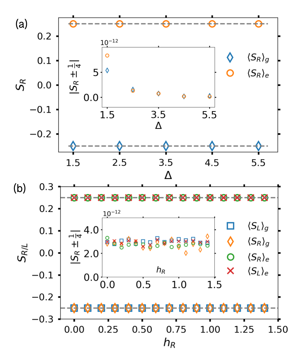
Figure 3: Edge spin accumulation ${\cal S}_{L/R}=\langle{\cal\hat{S}}^{z}_{L/R}\rangle$ in the ground state $|g\rangle$, with total spin $S^{z}=-\frac{1}{2}$, and in the midgap state $|e\rangle$, with total spin $S^{z}=\frac{1}{2}$. The model parameters used are (a) $N=1001$, $h_{R}=h_{L}=0.2$ with varying $\Delta$. (b) $N=1001$, $h_{L}=0$ and $\Delta=3$ with varying $h_{R}$. The dashed grey lines are on the curve $S=\pm 1/4$ to represent the expected value. Insets show the difference of numerical values from the expected value, which is on the order of the DMRG accuracy $\sim 10^{-12}$.

Variance.

We also calculated the spin variance to directly verify that the quarter spins found so far are sharp quantum observables. To this end we define the spin variance at, say, the left edge for a finite system $N$ and cutoff $\alpha$ as

$$\delta{\cal S}^{2}_{L}(N,\alpha)=\langle{\cal S}_{L}^{z}(N,\alpha)^{2}\rangle-\langle S_{L}^{z}(N,\alpha)\rangle^{2},$$ (15)

where the average is taken in either the ground state or the midgap state $|g\rangle$ and $|e\rangle$. In the thermodynamic limit, the variance as defined in Eq.(10), is then obtained as

$$\delta S_{L}^{2}\equiv\lim_{\alpha\rightarrow 0}\lim_{N\to\infty}\delta S^{2}(N,\alpha).$$ (16)

Taking the $N\rightarrow\infty$ is challenging and we circumvent this issue by assuming an ansatz relating $\delta S^{2}_{L}(N,\alpha)$ and $\delta S^{2}_{L}(\infty,\alpha)$

$$\delta S^{2}_{L}(N,\alpha)=\delta S^{2}(\infty,\alpha)-\frac{A}{\Delta}\alpha e^{-B\alpha N}.$$ (17)

With the above ansatz $\delta S^{2}_{L}=\lim_{\alpha\rightarrow 0}S(\infty,\alpha)=0$, and we can hence calculate $\delta S^{2}_{L}$ without taking explicitly the thermodynamic limit. We have verified this ansatz by taking the difference of $\delta S^{2}_{L}(N,\alpha)$ for different $N$’s. This is shown in Fig.4, where one can see that the ansatz fits the data very well. The fitted parameter $B\approx 2$ is nearly independent of the boundary fields, while $A$ takes a non-universal value.

In summary we find that in the low energy subspace spanned by the ground state $|g\rangle$ and the midgap state $|e\rangle$ one can assign to the left and the right edges a fractional spin state with eigenvalues ${\cal S}_{{L},{R}}=\pm\frac{1}{4}$. On the basis of our results we find it safe to expect that this is to be the case irrespective of the anisotropy parameter $\Delta>1$ and the values of the edge fields $[h_{L,R}|<\Delta-1$. Due to the zero variance of the fractional spin operators (12), the quarter spins ${\cal S}_{{L},{R}}$ are not simple quantum averages of half-integers spins at different sites but rather sharp quantum observables. The orientations of these quarter spins depend on the boundary fields and on the parity of the number of sites $N$ in such a way that (8) is satisfied in all ground states. Since the fractional spins at each edge are good quantum numbers we may then label the ground state and the midgap state as $|g(e)\rangle=|{\cal S}_{{L}},{\cal S}_{{R}}\rangle$. For odd $N$ spin chains these states are given by $|\pm 1/4,\pm 1/4\rangle$ whereas for even chains they are given by $|\pm 1/4,\mp 1/4\rangle$. One can easily verify that the total spin is $S^{z}=\pm 1/2$ and $S^{z}=0$ for the odd and even cases.

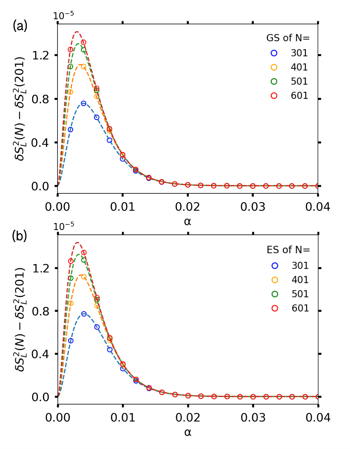
Figure 4: Edge spin variance $\delta S_{L}^{2}(N,\alpha)$ in (a) the ground state (GS) $S^{z}=-\frac{1}{2}$ and (b) the midgap state (ES) $S^{z}=\frac{1}{2}$ with model parameters $\Delta=3$, $h_{L}=h_{R}=0.2$ and varying $N$.

We want to point out that the existence of a gap above the ground state and the midgap state seems to be crucial for the quarter spins to be sharp quantum observables. Indeed, in the limit $\Delta\rightarrow 1$ where the mass gap goes to zero, we end up with the $XXX$ Heisenberg chain. In this case it was found in Pasnoori et al. (2023) that although the fractional spin $\pm 1/4$ exist in the ground state, their variance is not zero and hence the fractional spins are not genuine quantum observables.

IV Discussion

The first natural question that arises is whether or not the quarter spins found so far survive in the higher excited states of the spectrum of the XXZ chain. However, excited states above the midgap state contain propagating spinons. In such case, even if a quarter spin can be defined on average, we do not expect its variance to be zero as found for the XXX spin chain with edge fields Pasnoori et al. (2023). Another related question is whether these quarter spins survive edge fields higher than the critical value $h_{c}=\Delta-1$. In this regimes there are no midgap states Skorik and Saleur (1995); S.Skorik and A.Kapustin (1995); Grijalva et al. (2019); Nassar and Tirkkonen (1998) but we believe that sharp quarter spins exist in the ground state due to the existence of the spectral gap.

We shall end by commenting about the relation between the quarter spins found in this work with spontaneous symmetry breaking of the $\mathbb{Z}_{2}$ symmetry in the case of zero edge fields, i.e: $h_{L}=h_{R}=0$. In the limit of zero edge fields the two states $|g(e)\rangle$ become degenerate in the thermodynamical limit as the bound state energies (3) vanish. Without loss of generality one may then choose $|g\rangle=|-1/4,-1/4\rangle$ for $N$ odd and $|g\rangle=|1/4,-1/4\rangle$ for $N$ even. The two linear combinations $|\pm\rangle=(|g\rangle\pm|e\rangle)/\sqrt{2}$ are eigenstates of $\tau$, i.e: $\tau|\pm\rangle=\pm|\pm\rangle$. Since, in the same limit each of the two states $|g(e)\rangle$ are eigenstates of ${\hat{S}}^{z}_{L,R}$, the fractional spin operators map the two states $|\pm\rangle$ onto each other, i.e: ${\hat{S}}^{z}_{L,R}|\pm\rangle=(-1)^{N}\frac{1}{4}|\mp\rangle$. Hence the fractional spin operators are zero energy modes (ZEM) in the basis $|g\rangle$ and $|e\rangle$. Notice that, since in this subspace ${\hat{S}}^{z}_{L,R}$ are not independent as ${\hat{S}}^{z}_{L}=\pm{\hat{S}}^{z}_{R}$ in both states, there exits only one ZEM say ${\hat{S}}^{z}_{L}$. At this point it is worth mentioning that the hamiltonian (1) displays the remarkable property, discovered by P. FendleyFendley (2016), of having a strong zero energy mode $\Psi_{F}$ in the thermodynamical limit satisfying the following properties

$$[\Psi_{F},H]=0,\,\,\,\{\Psi_{F},\tau\}=0,\,\,\,\Psi_{F}^{2}=1.$$ (18)

The existence of the later operator insure that in the $N\rightarrow\infty$ limit the Hilbert space associated with the XXZ spin chain fractionalizes into two degenerated towers with eigenvalues $\tau=\pm 1$ which are mapped onto each other by the action of $\Psi_{F}$. We may therefore conclude that when projected in the low energy subspace spanned by the ground state and the midgap state the Fendley operator identifies with the fractional spin operator

$$\Psi_{F}\equiv 4{\hat{S}}^{z}_{L}.$$ (19)

Of course, since we do not expect a quarter fractional spin to be sharp in all the excited states, ${\hat{S}}^{z}_{L}$ is not a strong ZEM in contrast with the Fendley operator $\Psi_{F}$ but rather a soft ZEM. We finally notice that, following the same lines of arguments as given above, the fractional spin ${\hat{S}}^{z}_{L}$ is also a soft ZEM on the two lines $h_{L}=h_{R}$ for $N$ even and $h_{L}=-h_{R}$ for $N$ odd where the symmetries $\mathbb{P}\circ\mathbb{Z}_{2}$ and $\mathbb{P}$ are spontaneously broken. It would interesting to know if a strong zero mode similar to (18) exists on these two symmetric lines. We hope that the quarter spins found in this work could be probed in experiments using ultra cold atoms in optical lattices Duan et al. (2003).

Appendix A Even N DMRG

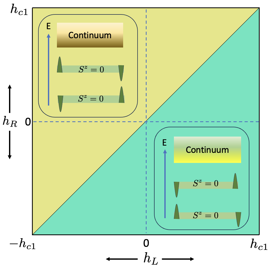
Figure 5: Ground state phase diagram of the XXZ model with edge fields smaller than the critical field $|h_{L,R}|<h_{c}=\Delta-1$ and for an even number of sites. The ground state as well as the first excited state which is a midgap state have total spin $S^{z}=0$. Both states host fractional quarter spins ${\cal S}_{L,R}=\pm 1/4$ at both edges of the chain. These fractional spins are sharp quantum observables which reconstruct the total spin of each state $S^{z}={\cal S}_{L}+{\cal S}_{R}=0$. The $\pm 1/4$ quarter spins are depicted by triangles pointing upward and downward respectively. On the separatrix $h_{L}-h_{R}=0$ the two states are degenerate and the edge spin operator become a zero energy mode.

A.1 Edge spin accumulation

The lowest-energy state of the XXZ Hamiltonian defined in Eqn.(1) can be solved numerically in a matrix product (MPS) form by the density matrix renormalization group (DMRG) method. The magnetization at site $j$ can be computed as $S^{z}_{j}=\frac{1}{2}\langle\psi|\sigma^{z}_{x}|\psi\rangle$. Also, we define an Ansatz for the spin profile as

$$\begin{split}S^{z}_{j}=&\Delta S^{z}(j)+\frac{1}{2}\sigma(\Delta)(-1)^{x}\end{split}$$ (20)

with $\sigma(\Delta)$ is the bulk staggered magnetization for a periodic $XXZ$ chain with anisotropy $\Delta$. The numerical results for the validity of fitting in the lowest two excited states are shown in Figs.(6,7) for even cites and in Figs.(2) for the odd sites.

With the definition of the edge spin accumulation as

$${\cal S}_{L}=\lim_{\alpha\to 0}\lim_{N\to\infty}\sum_{j}e^{-\alpha x}S^{z}(j,N)=\lim_{\alpha\to 0}\lim_{N\to\infty}S^{z}_{L}(N,\alpha),$$ (21)

then ${\cal S}_{L/R}=\pm\frac{1}{4}$ in both of the two lowest energy states, and they sum up to ${\cal S}_{L}+{\cal S}_{R}=S^{z}$. Noticing, that the non-converging part is the bulk magnetization if we want to define the edge spin accumulation on a finite system, we introduce the quantity $S_{\alpha}=\pm\frac{1}{4}=\sum_{x}\Delta S_{\alpha}^{z}(x)\pm\frac{1}{2}\sigma(\Delta)$ with $\alpha=L,R$. The edge spin accumulation is shown in Fig.(8) for a chain with even number of sites and Fig.(3) for a chain with odd number of sites.

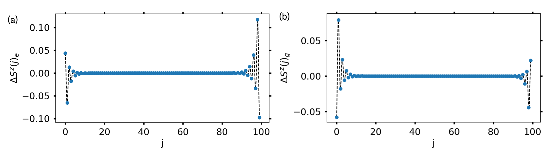
Figure 6: Spin profile $\Delta S^{z}(j)$ and the fitting of ansatz (a) in the ground state $|e\rangle$ (b) in the midgap state $|g\rangle$ with model parameters $N=100$, $h_{L}=0.1,h_{R}=0.5$ and for $\Delta=3$.

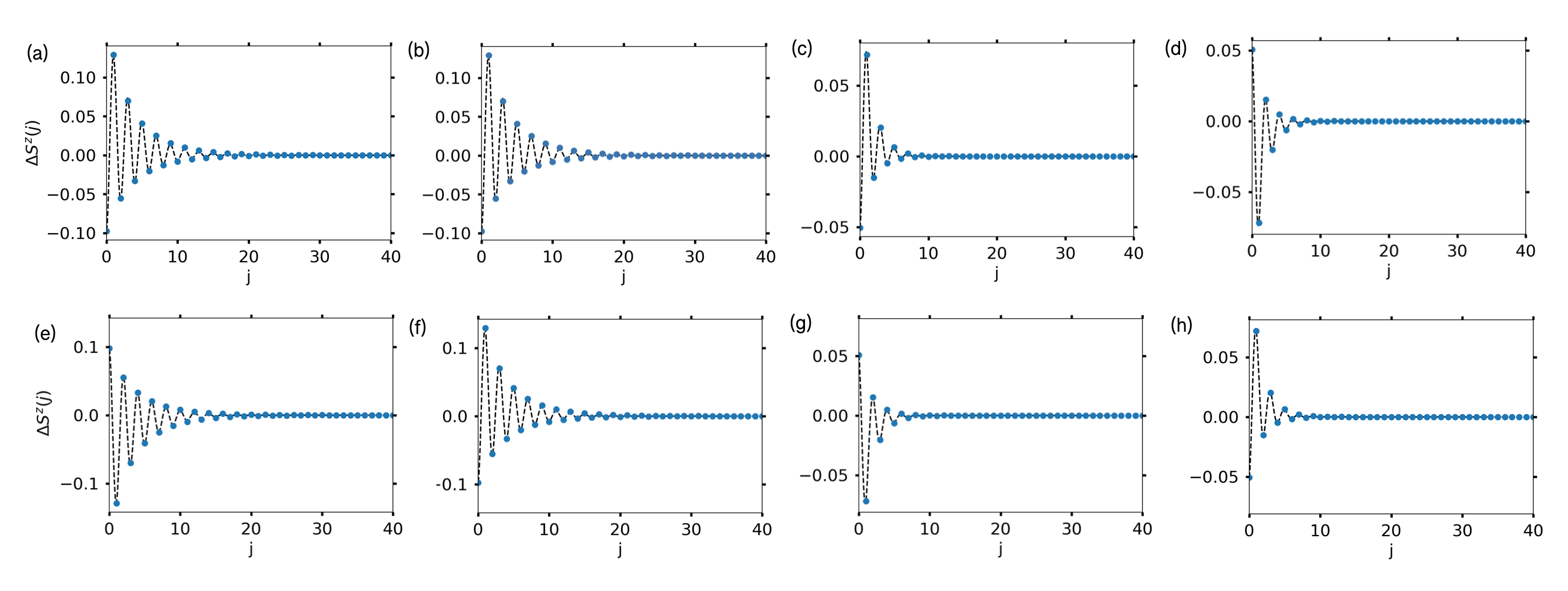
Figure 7: Spin profile on the left hand side $\Delta S^{z}_{L}(j)$ of the two degenerated ground states without the presence of magnetic field $h_{L}=h_{R}=0$ for system size $N=1001$ and (a,b) $\Delta=2$ and (c,d) $\Delta=3$. Spin profile on the left hand side $\Delta S^{z}_{L}(j)$ of the two degenerated ground states without the presence of magnetic field $h_{L}=h_{R}=0$ for system size $N=1000$ and (e,f) $\Delta=2$ and (g,h) $\Delta=3$.

A.2 Edge Spin Variance

Defining the spin variance operator at the edge for a finite system $N$ and cutoff $\alpha$ as

$$\delta S^{2}_{L}(N,\alpha)=\langle S_{L}^{z}(N,\alpha)^{2}\rangle-\langle S_{L}^{z}(N,\alpha)\rangle^{2}.$$ (22)

The thermodynamic spin variance is defined through the same limit as in Eq.(21), and the condition that the fractional spin ${\cal S}_{L/R}$ is a sharp quantum observable is that the variance vanishes:

$$\delta S^{2}_{L}\equiv\lim_{\alpha\to\infty}\lim_{N\to\infty}\delta S_{L}^{2}(N,\alpha)=0.$$ (23)

Taking the limit $N\rightarrow\infty$ is challenging, and we circumvent this issue by assuming an ansatz relating $\delta S^{2}_{L}(N,\alpha)$ and $\delta S^{2}_{L}(\infty,\alpha)$

$$\delta S^{2}_{L}(N,\alpha)=\delta S_{L}^{2}(\infty,\alpha)-\frac{A}{\Delta}\alpha e^{-B\alpha L}.$$ (24)

Then, $\delta S^{2}_{L}=\lim_{\alpha\rightarrow 0}S(\infty,\alpha)$, and we can calculation the value of $\delta S^{2}_{L}$ in the thermodynamic limit. We verify this ansatz by taking the difference of $\delta S^{2}_{L}(N,\alpha)$ for different $N$’s. This is shown in Fig.(9) for even chain and Fig.(4) for odd chain, where one can see that the ansatz fits the data very well.

Therefore, the thermodynamic limit of the variance does vanish, $\delta S^{2}=0$, and the edge spin is indeed a well-defined quantum observable.

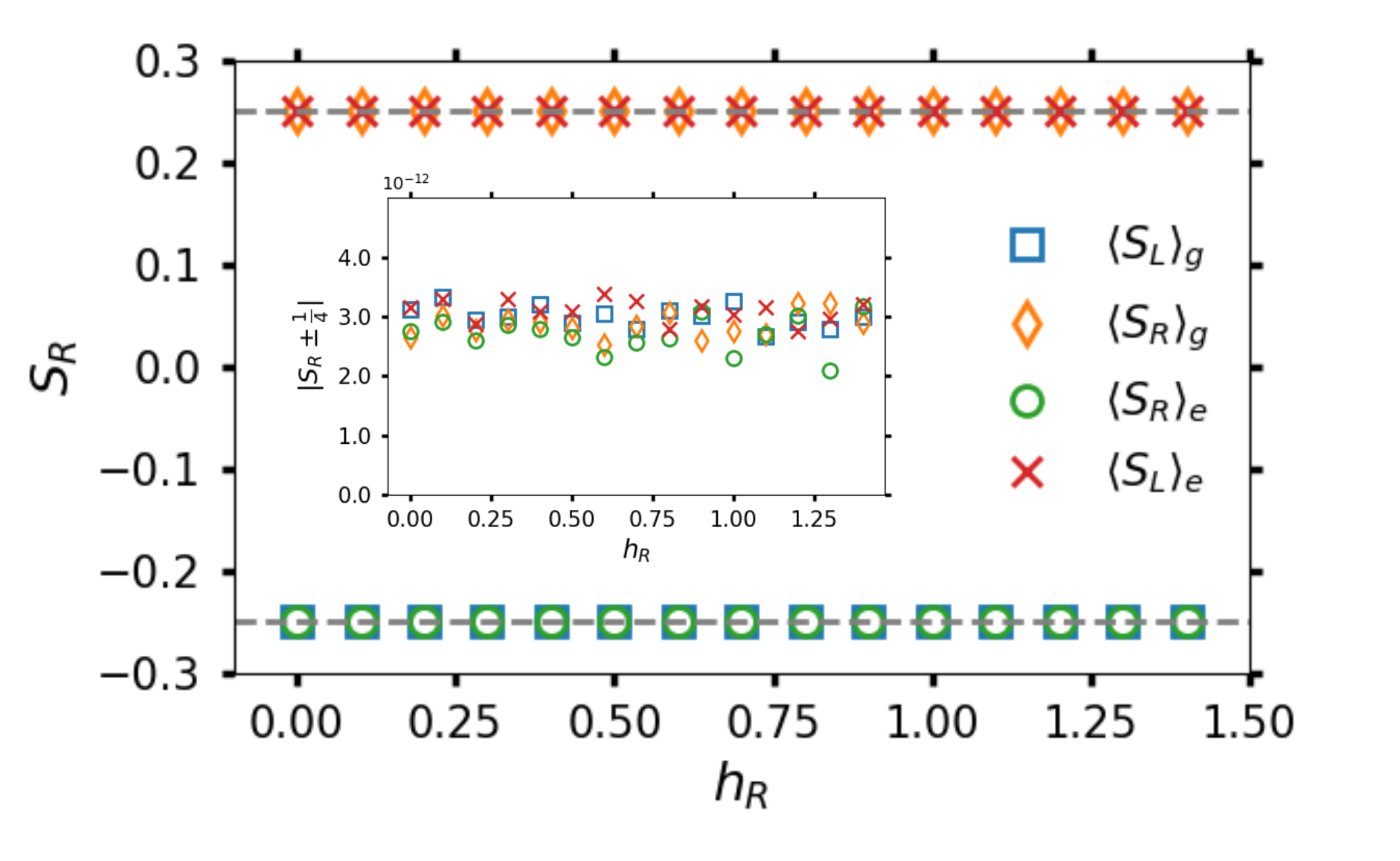
Figure 8: Edge spin accumulation ${\cal\hat{S}}_{\cal L/\cal R}=\langle{\cal\hat{S}}^{z}_{\cal L/\cal R}\rangle$ in the ground state $|g\rangle$, and in the midgap state $|e\rangle$. The model parameters used are $N=1000$, $h_{\cal L}=0$ and $\Delta=3$ with varying $h_{\cal R}$.

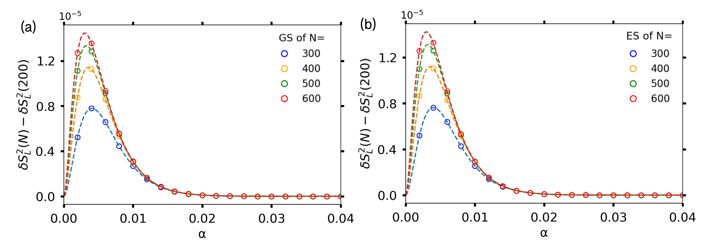
Figure 9: Edge spin variance $\delta S_{\cal L}^{2}(N,\alpha)$ in (a) the ground state $S^{z}=-\frac{1}{2}$ and (b) the midgap state $S^{z}=\frac{1}{2}$ with model parameters $\Delta=3$, $h_{\cal L}=h_{\cal R}=0.2$ and varying $N$.

Appendix B Bethe Ansatz

B.1 Hamiltonian

Recalling the Hamiltonian of the system:

$$H=\sum_{j=1}^{N-1}\left[\sigma^{x}_{j}\sigma^{x}_{j+1}+\sigma^{y}_{j}\sigma^{y}_{j+1}+\Delta(\sigma^{z}_{j}\sigma^{z}_{j+1}-1)\right]$$

$$+h_{L}\sigma^{z}_{1}+h_{R}\sigma^{z}_{N},$$ (25)

where $h_{L},h_{R}$ are magnetic fields at the left and the right edges respectively. We can introduce new parameters $\gamma$, $h_{c1}$, $h_{c2}$ such that

$$\Delta=\cosh\gamma,\gamma>0,\;\;\;\;\;h_{c1}=\Delta-1,\;\;\;\;\;h_{c2}=\Delta+1$$ (26)

The Bethe equations can be obtained by following the method of coordinate or algebraic Bethe ansatz Alcaraz et al. (1987); Sklyanin (1988); Wang et al. (2015). One obtains the following Bethe equations for the reference state with all spin up

$$\left(\frac{\sin\frac{1}{2}(\lambda_{j}-i\gamma)}{\sin\frac{1}{2}(\lambda_{j}+i\gamma)}\right)^{2N}\prod_{\alpha}^{L,R}\left(\frac{\sin\frac{1}{2}(\lambda_{j}+i\gamma(1+\epsilon_{\alpha}))}{\sin\frac{1}{2}(\lambda_{j}+i\gamma(1+\epsilon_{\alpha}))}\right)$$

$$=\prod_{\sigma=\pm}\prod_{k=1}^{M}\left(\frac{\sin\frac{1}{2}(\lambda_{j}+\sigma\lambda_{k}-2i\gamma)}{\sin\frac{1}{2}(\lambda_{j}+\sigma\lambda_{k}+2i\gamma)}\right)$$ (27)

where

$$h_{\alpha}=-\sinh\gamma\coth(\frac{\epsilon_{\alpha}\gamma}{2}),\;\;\;\epsilon_{\alpha}=\tilde{\epsilon}_{\alpha}+i\delta_{\alpha}\frac{\pi}{\gamma},$$

$$\delta_{\alpha}=\begin{cases}1&|h_{\alpha}|<\sinh\gamma\\ 0&|h_{\alpha}|>\sinh\gamma\end{cases}$$ (28)

Note that $h_{c1}<\sinh\gamma<h_{c2}$. The Bethe equations for reference state with all spin down can be obtained by the transformation $\epsilon_{\alpha}\rightarrow-\epsilon_{\alpha}$ Sklyanin (1988). The energy of a state described by the set of Bethe roots $\lambda_{j}$ is given by

$$E=\frac{1}{2}\left[(N-1)\cosh\gamma+h_{L}+h_{R}\right]$$

$$-2\sinh\gamma\sum_{j=1}^{M}\frac{\sinh\gamma}{\cosh\gamma-\cos\lambda_{j}}$$ (29)

The boundary magnetic fields break the $\mathbb{Z}_{2}$ spin flip symmetry. Under the spin flip of all the sites, the bulk remains invariant but the boundary terms remain invariant only after the direction of both the magnetic fields is reversed, hence we have the following isometry

$$\prod_{i=1}^{N}\sigma^{x}_{i}H\sigma^{x}_{i},\;\;h_{L}\rightarrow-h_{L},\;\;h_{R}\rightarrow-h_{R}.$$ (30)

B.2 Bethe Solution

In this section we construct the ground states and the boundary excitations with the lowest energy in each of the four sub-phases $A_{j=(1,2,3,4)}$, corresponding to the domains of the boundary fields $(0\leq h_{L}\leq h_{c1},0\leq h_{R}\leq h_{c1}),(0\geq h_{L}\geq-h_{c1},0\leq h_{R}\leq h_{c1}),(0\geq h_{L}\geq-h_{c1},0\geq h_{R}\geq-h_{c1})$ and $(0\leq h_{L}\leq h_{c1},0\geq h_{R}\geq-h_{c1})$ respectively.

B.2.1 Region $A_{1}$: odd number of sites

The region $A_{1}$ corresponds to the following values of the boundary magnetic fields: $0<h_{L},h_{R}<h_{c1}$. This corresponds to $\epsilon_{\alpha}=-\tilde{\epsilon}_{\alpha}+i\pi$, with $\tilde{\epsilon}_{\alpha}<1$, $\alpha=L,R$.

First consider the state with all real $\lambda$, which take values between $(-\pi,\pi]$. Applying logarithm to B.1 we obtain

$$2N\varphi(\lambda_{j},1)-\sum_{\alpha=L,R}\varphi(\lambda_{j},1-\tilde{\epsilon}_{\alpha})+\varphi(\lambda_{j},1)+\varphi^{\prime}(\lambda_{j},1)=2\pi I_{j}+\sum_{\sigma=\pm}\sum_{k\neq j}\varphi(\lambda_{j}+\sigma\lambda_{k},2).$$

where

$$\varphi(x,y)=\ln\left(\frac{\sin\frac{1}{2}(x-i\gamma y)}{\sin\frac{1}{2}(x+i\gamma y)}\right),\;\;\;\;\varphi^{\prime}(x,y)=\ln\left(\frac{\cos\frac{1}{2}(x-i\gamma y)}{\cos\frac{1}{2}(x+i\gamma y)}\right).$$ (32)

We define the counting function $\nu(\lambda)$ such that $\nu(\lambda_{j})=I_{j}$. Differentiating B.2.1 and using $\frac{d}{d\lambda}\nu(\lambda)=\rho(\lambda)$, we obtain

$$(2N+1)a(\lambda,1)-\sum_{\alpha=L,R}a(\lambda-\pi,1-\tilde{\epsilon}_{\alpha})+a(\lambda-\pi,1)-2\pi\delta(\lambda)-2\pi\delta(\lambda-\pi)=2\pi\rho(\lambda)+\sum_{\sigma=\pm}\int a(\lambda+\sigma\mu,2)\rho(\mu)d\mu,$$

where we have removed the solutions $\lambda=0,\pi$ as they lead to a vanishing wavefunction Skorik and Saleur (1995). Here

$$a(x,y)=\frac{\sinh(\gamma y)}{\cosh(\gamma y)-\cos(\lambda)}.$$ (34)

The above equation can be solved by applying Fourier transform

$$f(x)=\sum_{k=-\infty}^{\infty}\hat{f}(\omega)e^{i\omega x},\;\;\;\;\;\;\;\;\hat{f}(\omega)=\frac{1}{2\pi}\int_{-\pi}^{\pi}f(x)e^{-i\omega x}dx.$$ (35)

Using $\hat{a}(\omega,y)=e^{-\gamma y|\omega|}$, we obtain the following density distribution for the state with all real roots

$$\hat{\rho}_{\left|\frac{1}{2}\right>_{A_{1}}}(\omega)=\frac{(2N+1)e^{-\gamma|\omega|}+(-1)^{\omega}e^{-\gamma|\omega|}-(1+(-1)^{\omega})-\sum_{\alpha=L,R}(-1)^{\omega}e^{-\gamma(1-\tilde{\epsilon}_{\alpha})|\omega|}}{4\pi(1+e^{-2\gamma|\omega|})}.$$ (36)

The reason for the subscripts will become evident when we find the spin $S^{z}$ of the state. The number of Bethe roots can be obtained by using the relation

$$M=\int_{-\pi}^{\pi}\rho(\lambda)d\lambda.$$ (37)

The total spin $S^{z}$ of the state can be found using the relation $S^{z}=\frac{N}{2}-M$. Using 36 in the above relations we find that the total spin $S^{z}$ of the state described by the distribution $\hat{\rho}_{\left|\frac{1}{2}\right>_{A_{1}}}(\omega)$ is $S^{z}=\frac{1}{2}$. We denote this state by $\left|\frac{1}{2}\right>_{A_{1}}$.

By starting with the Bethe equations corresponding to all spin down reference state we have

$$(2N+1)a(\lambda,1)-\sum_{\alpha=L,R}a(\lambda-\pi,1+\tilde{\epsilon}_{\alpha})+a(\lambda-\pi,1)-2\pi\delta(\lambda)-2\pi\delta(\lambda-\pi)=2\pi\rho(\lambda)+\sum_{\sigma=\pm}\int a(\lambda+\sigma\mu,2)\rho(\mu)d\mu$$

Following the same procedure as above, we obtain the following distribution for a state with all real $\lambda$

$$\hat{\rho}_{\left|-\frac{1}{2}\right>_{A_{1}}}(\omega)=\frac{(2N+1)e^{-\gamma|\omega|}+(-1)^{\omega}e^{-\gamma|\omega|}-(1+(-1)^{\omega})-\sum_{\alpha=L,R}(-1)^{\omega}e^{-\gamma(1+\tilde{\epsilon}_{\alpha})|\omega|}}{4\pi(1+e^{-2\gamma|\omega|})}.$$ (39)

The total spin $S^{z}$ of this state is $S^{z}=-\frac{1}{2}$. We denote this state by $\left|-\frac{1}{2}\right>_{A_{1}}$.

Using B.1 we can calculate the energy difference between the two states $\left|\frac{1}{2}\right>_{A_{1}}$ and $\left|-\frac{1}{2}\right>_{A_{1}}$.

We have

$$E_{\left|\frac{1}{2}\right>_{A_{1}}}-E_{\left|-\frac{1}{2}\right>_{A_{1}}}=h_{L}+h_{R}-2\sinh\gamma\sum_{\alpha=L,R}\int_{-\pi}^{\pi}a(\lambda,1)\;\delta\rho_{\tiny{\left|\frac{1}{2}\right>,\left|-\frac{1}{2}\right>}}(\lambda)d\lambda,$$ (40)

where $\delta\rho_{\tiny{\left|\frac{1}{2}\right>,\left|-\frac{1}{2}\right>}}(\lambda)$ is the difference in the density distributions of the states $\left|\frac{1}{2}\right>_{A_{1}}$ and $\left|-\frac{1}{2}\right>_{A_{1}}$. The expression 40 can be written as

$$E_{\left|\frac{1}{2}\right>_{A_{1}}}-E_{\left|-\frac{1}{2}\right>_{A_{1}}}=h_{L}+h_{R}+4\pi\sinh\gamma\sum_{\omega=-\infty}^{\infty}\hat{a}(\omega,1)\Delta\hat{\rho}_{\tiny{\left|\frac{1}{2}\right>,\left|-\frac{1}{2}\right>}}(\omega).$$ (41)

Using 36 and 39 in the above expression we obtain

$$E_{\left|\frac{1}{2}\right>_{A_{1}}}-E_{\left|-\frac{1}{2}\right>_{A_{1}}}=h_{L}+h_{R}+\sinh\gamma\sum_{\alpha=L,R}\sum_{\omega=-\infty}^{\infty}(-1)^{\omega}\;\frac{\sinh(\gamma\tilde{\epsilon}_{\alpha}|\omega|)}{\cosh(\gamma\omega)}e^{-\gamma|\omega|},$$ (42)

which can be written as

$$E_{\left|\frac{1}{2}\right>_{A_{1}}}-E_{\left|-\frac{1}{2}\right>_{A_{1}}}=m_{L}+m_{R},$$ (43)

where

$$m_{\alpha}=h_{\alpha}+\sinh\gamma\sum_{\omega=-\infty}^{\infty}(-1)^{\omega}\;\frac{\sinh(\gamma\tilde{\epsilon}_{\alpha}|\omega|)}{\cosh(\gamma\omega)}e^{-\gamma|\omega|}.$$ (44)

The ground state is $\left|-\frac{1}{2}\right>_{A_{1}}.$

B.2.2 Region $A_{1}$: Even number of sites

The Bethe equations corresponding to all spin up reference state have two boundary string solutions $\lambda_{bs\alpha}=\pi+\pm i\gamma(1-\tilde{\epsilon}_{\alpha})$, $\alpha=L,R$ . Adding either of these two boundary strings to the Bethe equations B.1 and taking logarithm we obtain

$$2N\varphi(\lambda_{j},1)-\sum_{\alpha=L,R}\varphi(\lambda_{j}-\pi,1-\tilde{\epsilon}_{\alpha})+\varphi(\lambda_{j},1)+\varphi^{\prime}(\lambda_{j},1)-\varphi(\lambda,(3-\tilde{\epsilon}_{\beta}))-\varphi(\lambda,(1+\tilde{\epsilon}_{\beta}))$$

$$=2\pi I_{j}+\sum_{\sigma=\pm}\sum_{k\neq j}\varphi(\lambda_{j}+\sigma\lambda_{k},2),$$ (45)

where $\beta$ is either $L$ or $R$. Differentiating the above equation with respect to $\lambda$ and taking the Fourier transform we obtain

$$\tilde{\rho}_{\left|0\right>_{\beta A_{1}}}(\omega)=\tilde{\rho}_{\left|\frac{1}{2}\right>_{A_{1}}}(\omega)+\Delta\tilde{\rho}_{\beta}(\omega),$$ (46)

where

$$\Delta\tilde{\rho}_{\beta}(\omega)=-\frac{1}{4\pi}(-1)^{\omega}\frac{e^{-\gamma(3-\tilde{\epsilon}_{\beta})|\omega|}+e^{-\gamma(1+\tilde{\epsilon}_{\beta})|\omega|}}{1+e^{-2\gamma|\omega|}}.$$ (47)

The spin of the state containing this boundary string can be calculated using $S^{z}=\frac{N}{2}-M$, where

$$M=1+\int_{-\pi}^{\pi}\rho_{\left|0\right>_{\beta A_{1}}}(\lambda)d\lambda.$$ (48)

We obtain $S^{z}_{\left|0\right>_{\beta A_{1}}}=0$, $\beta=L,R$. Hence there are two states with $S^{z}=0$ that correspond to the presence of the boundary strings $\lambda_{bsL}$ and $\lambda_{bsR}$.

The energy of the boundary string can be calculated using B.1. We have

$$E_{\lambda_{bs\beta}}=-\frac{2\sinh^{2}\gamma}{\cosh\gamma+\cosh\gamma(1-\tilde{\epsilon}_{\beta})}-2\sinh\gamma\int_{-\pi}^{\pi}a(\lambda-\pi,1)\Delta\rho_{\beta}(\lambda)d\lambda.$$ (49)

Using 46 and evaluating the integral one obtains,

$$E_{\lambda_{bs\beta}}=-\frac{2\sinh^{2}\gamma}{\cosh\gamma+\cosh\gamma(1-\tilde{\epsilon}_{\beta})}+\sinh\gamma\sum_{\omega}(-1)^{\omega}e^{-2\gamma|\omega|}\frac{\cosh(\gamma(1-\tilde{\epsilon}_{\beta})\omega)}{\cosh(\gamma\omega)}=-m_{\beta}.$$ (50)

Hence the ground state is either $\left|0\right>_{L,A_{1}}$ or $\left|0\right>_{R,A_{1}}$ depending on the values of $h_{L},h_{R}$.

B.2.3 $A_{2}$: Odd number of sites

The region $A_{2}$ corresponds to the following values of the boundary magnetic fields: $0<h_{R}<h_{c1}$, $-h_{c1}<h_{L}<0$. In this region the logarithmic form of the Bethe equations can be obtained from B.2.1 by the transformation $\tilde{\epsilon}_{L}\rightarrow-\tilde{\epsilon}_{L}$. We have

$$(2N+1)a(\lambda,1)-a(\lambda-\pi,1-\tilde{\epsilon}_{R})-a(\lambda-\pi,1+\tilde{\epsilon}_{L})+a(\lambda-\pi,1)-2\pi\delta(\lambda)-2\pi\delta(\lambda-\pi)$$

$$=2\pi\rho(\lambda)+\sum_{\sigma=\pm}\int a(\lambda+\sigma\mu,2)\rho(\mu)d\mu.$$ (51)

Taking Fourier transform we obtain

$$\hat{\rho}_{\left|\frac{1}{2}\right>_{A_{2}}}(\omega)=\frac{(2N+1)e^{-\gamma|\omega|}+(-1)^{\omega}e^{-\gamma|\omega|}-(1+(-1)^{\omega})-(-1)^{\omega}e^{-\gamma(1-\tilde{\epsilon}_{R})|\omega|}-(-1)^{\omega}e^{-\gamma(1+\tilde{\epsilon}_{L})|\omega|}}{4\pi(1+e^{-2\gamma|\omega|})}.$$ (52)

The number of Bethe roots can be obtained by using the relation

$$M=\int_{-\pi}^{\pi}\rho(\lambda)d\lambda.$$ (53)

The total spin $S^{z}$ of the state can be found using the relation $S^{z}=\frac{N}{2}-M$. Using 52 in the above relations we find that the total spin $S^{z}$ of the state described by the distribution $\hat{\rho}_{\left|\frac{1}{2}\right>_{A_{2}}}(\omega)$ is $S^{z}=\frac{1}{2}$. We denote this state by $\left|\frac{1}{2}\right>_{A_{2}}$.

By starting with the Bethe equations corresponding to all spin down reference state we have

$$(2N+1)a(\lambda,1)-a(\lambda-\pi,1+\tilde{\epsilon}_{R})-a(\lambda-\pi,1-\tilde{\epsilon}_{L})+a(\lambda-\pi,1)-2\pi\delta(\lambda)-2\pi\delta(\lambda-\pi)$$

$$=2\pi\rho(\lambda)+\sum_{\sigma=\pm}\int a(\lambda+\sigma\mu,2)\rho(\mu)d\mu.$$ (54)

Following the same procedure as above, we obtain the following distribution for a state with all real $\lambda$

$$\hat{\rho}_{\left|-\frac{1}{2}\right>_{A_{1}}}(\omega)=\frac{(2N+1)e^{-\gamma|\omega|}+(-1)^{\omega}e^{-\gamma|\omega|}-(1+(-1)^{\omega})-(-1)^{\omega}e^{-\gamma(1+\tilde{\epsilon}_{R})|\omega|}-(-1)^{\omega}e^{-\gamma(1-\tilde{\epsilon}_{L})|\omega|}}{4\pi(1+e^{-2\gamma|\omega|})}.$$ (55)

The total spin $S^{z}$ of this state is $S^{z}=-\frac{1}{2}$. We denote this state by $\left|-\frac{1}{2}\right>_{A_{2}}$.

Using B.1 we can calculate the energy difference between the two states $\left|\frac{1}{2}\right>_{A_{2}}$ and $\left|-\frac{1}{2}\right>_{A_{2}}$.

We have

$$E_{\left|\frac{1}{2}\right>_{A_{2}}}-E_{\left|-\frac{1}{2}\right>_{A_{2}}}=-h_{L}+h_{R}-2\sinh\gamma\sum_{\alpha=L,R}\int_{-\pi}^{\pi}a(\lambda,1)\;\delta\rho_{\tiny{\left|\frac{1}{2}\right>,\left|-\frac{1}{2}\right>}}(\lambda)d\lambda,$$ (56)

where $\delta\rho_{\tiny{\left|\frac{1}{2}\right>,\left|-\frac{1}{2}\right>}}(\lambda)$ is the difference in the density distributions of the states $\left|\frac{1}{2}\right>$ and $\left|-\frac{1}{2}\right>$. The expression 56 can be written as

$$E_{\left|\frac{1}{2}\right>_{A_{2}}}-E_{\left|-\frac{1}{2}\right>_{A_{2}}}=-h_{L}+h_{R}+4\pi\sinh\gamma\sum_{\omega=-\infty}^{\infty}\hat{a}(\omega,1)\Delta\hat{\rho}_{\tiny{\left|\frac{1}{2}\right>,\left|-\frac{1}{2}\right>}}(\omega).$$ (57)

Using 52 and 55 in the above expression we obtain

$$E_{\left|\frac{1}{2}\right>_{A_{2}}}-E_{\left|-\frac{1}{2}\right>_{A_{2}}}=-h_{L}+h_{R}+\sinh\gamma(-1)^{\omega}\;\frac{\sinh(\gamma\tilde{\epsilon}_{R}|\omega|)}{\cosh(\gamma\omega)}e^{-\gamma|\omega|}-\sinh\gamma(-1)^{\omega}\;\frac{\sinh(\gamma\tilde{\epsilon}_{L}|\omega|)}{\cosh(\gamma\omega)}e^{-\gamma|\omega|},$$ (58)

which can be written as

$$E_{\left|\frac{1}{2}\right>_{A_{2}}}-E_{\left|-\frac{1}{2}\right>_{A_{2}}}=m_{R}-m_{L}.$$ (59)

Hence the ground state for odd number of sites is $\left|\pm\frac{1}{2}\right>_{A_{2}}$ depending on the values of $h_{L},h_{R}$.

B.2.4 $A_{2}$: Even number of sites

The Bethe equations corresponding to all spin up reference state have two boundary string solutions $\lambda_{bsR}=\pi\pm i\gamma(1-\tilde{\epsilon}_{R})$, $\lambda_{bsL^{\prime}}=\pi\pm i\gamma(1+\tilde{\epsilon}_{L})$. Adding $\lambda_{bsR}$ to the state $\left|\frac{1}{2}\right>_{A_{2}}$ leads to the state with following root distribution

$$\tilde{\rho}_{\left|0\right>_{\beta A_{2}}}(\omega)=\tilde{\rho}_{\left|\frac{1}{2}\right>_{A_{2}}}(\omega)+\Delta\tilde{\rho}_{R}(\omega),$$ (60)

where $\Delta\tilde{\rho}_{R}$ is given by 47 with $\beta=R$. The spin of the state containing this boundary string can be calculated using $S^{z}=\frac{N}{2}-M$, where

$$M=1+\int_{-\pi}^{\pi}\rho_{\left|0\right>_{RA_{2}}}(\lambda)d\lambda.$$ (61)

We obtain $S^{z}_{\left|0\right>_{RA_{2}}}=0$. The energy of the boundary string is given by 50, which is $-m_{R}$.

Adding the boundary string $\lambda_{bsL^{\prime}}$ to the state $\left|\frac{1}{2}\right>_{A_{2}}$, we obtain

$$\tilde{\rho}_{\left|0\right>_{L^{\prime}A_{2}}}(\omega)=\tilde{\rho}_{\left|\frac{1}{2}\right>_{A_{2}}}(\omega)+\Delta\tilde{\rho}_{L^{\prime}}(\omega),$$ (62)

where

$$\Delta\tilde{\rho}_{L^{\prime}}(\omega)=-\frac{1}{4\pi}(-1)^{\omega}\frac{e^{-\gamma(3+\tilde{\epsilon}_{L})|\omega|}+e^{-\gamma(1-\tilde{\epsilon}_{L})|\omega|}}{1+e^{-2\gamma|\omega|}}.$$ (63)

The spin of the state containing this boundary string can be calculated using $S^{z}=\frac{N}{2}-M$, where

$$M=1+\int_{-\pi}^{\pi}\rho_{\left|0\right>_{L^{\prime}A_{2}}}(\lambda)d\lambda.$$ (64)

We obtain $S^{z}_{\left|0\right>_{L^{\prime}A_{2}}}=0$. The energy of the boundary string $\lambda_{bsL^{\prime}}$ is given by

$$E_{\lambda_{bs\beta^{\prime}}}=-\frac{2\sinh^{2}\gamma}{\cosh\gamma+\cosh\gamma(1+\tilde{\epsilon}_{\beta})}+\sinh\gamma\sum_{\omega}(-1)^{\omega}e^{-2\gamma|\omega|}\frac{\cosh(\gamma(1+\tilde{\epsilon}_{\beta})\omega)}{\cosh(\gamma\omega)}=m_{\beta},$$ (65)

with $\beta=L$. The energy difference between the states $\left|0\right>_{L^{\prime}A_{2}}$ and $\left|0\right>_{RA_{2}}$ can be calculated similar to the previous section, we obtain

$$E_{\left|0\right>_{L^{\prime}A_{2}}}-E_{\left|0\right>_{RA_{2}}}=m_{L}+m_{R}.$$ (66)

Hence the ground state for even number of sites is $\left|0\right>_{RA_{2}}$.

B.2.5 $A_{3}$ and $A_{4}$ sub-phases

In constructing a state in the phase $A_{3}$ or $A_{4}$, we can use the construction of the respective state in the phase $A_{1}$ or $A_{2}$ respectively, and use the following transformation:

$$|\uparrow\uparrow...\uparrow\rangle\leftrightarrow|\downarrow\downarrow...\downarrow\rangle,\hskip 14.22636pth_{L}\rightarrow-h_{L},\hskip 11.38109pth_{R}\rightarrow h_{R},$$ (67)

where the all spin up and all spin down reference states are interchanged and the boundary magnetic fields change sign.

B.3 Summary of Bethe Solution

In this section we summarize the construction of the Bethe solution obtained above

B.3.1 Odd number of sites

The $A_{1}$ and $A_{3}$ sub-phases.

In these cases both boundary magnetic fields point towards the same direction: along the positive $z$ axis for the $A_{1}$ sub-phase and negative $z$ axis for the $A_{3}$ sub-phase. Both cases are related by the isometry (30). Qualitatively speaking, in the sub-phases $A_{1,3}$ and for $N$ odd, the boundary magnetic fields are not frustrating in the sense that in the Ising limit of (B.1) the ground-state would exhibit perfect antiferromagnetic order.

1) In the $A_{1}$ phase we find that the ground-state is unique and has a total spin $S^{z}=-\frac{1}{2}$. It is constructed by starting with all spin down reference state and contains $\frac{N-1}{2}$ real roots. This state is labelled by $\left|-\frac{1}{2}\right>_{A1}$.

2) In the $A_{1}$ phase, there exists an excited state with total spin $S^{z}=+\frac{1}{2}$, which does not contain any spinons. It is constructed by starting with all spin up reference state and contains $\frac{N-1}{2}$ real roots. This state is labelled by $\left|+\frac{1}{2}\right>_{A1}$.

3)The energy difference between these two states in the $A_{1}$ phase is

$$E_{\left|\frac{1}{2}\right>_{A_{1}}}-E_{\left|-\frac{1}{2}\right>_{A_{1}}}=m_{L}+m_{R}.$$ (68)

4) All the states in the $A_{3}$ phase can be obtained by using the symmetry 67 described above.

The $A_{2}$ and $A_{4}$ sub-phases.

In these cases the boundary fields are frustrating for $N$ odd in the sense discussed above.

1) In the $A_{2}$ phase, for $|h_{L}|<|h_{R}|$, the ground state has total spin $S^{z}=-\frac{1}{2}$. It is constructed by starting with all spin down reference state and contains $\frac{N-1}{2}$ real roots. This state is labelled as $\left|-\frac{1}{2}\right>_{A2}$.

2) In the $A_{2}$ phase, there exists an excited state with total spin $S^{z}=+\frac{1}{2}$, which does not contain any spinons. It is constructed by starting with all spin up reference state and contains $\frac{N-1}{2}$ real roots. This state is labelled by $\left|+\frac{1}{2}\right>_{A2}$.

3)The energy difference between these two states in the $A_{2}$ phase is

$$E_{\left|\frac{1}{2}\right>_{A_{2}}}-E_{\left|-\frac{1}{2}\right>_{A_{2}}}=m_{R}-m_{L}.$$ (69)

4) From the above expression, one can infer that in the $A_{2}$ phase, for $|h_{L}|>|h_{R}|$, the state $\left|+\frac{1}{2}\right>_{A2}$ is the ground state and the state $\left|-\frac{1}{2}\right>_{A2}$ is an excited state.

5) Using the symmetry 30, we can obtain all the states in the sub-phase $A_{4}$ from the states in the sub-phase $A_{2}$.

Phase diagram

Having obtained the solution in the region where $|h_{L,R}|<h_{c1}$ for odd number of sites chain, we can now obtain the phase diagram shown in the main text 1. The region which corresponds to $h_{R}+h_{L}>0$, can be divided into three regions: (a) $h_{R},h_{L}>0$ (b) $h_{R}>0,h_{L}<0,|h_{R}|>|h_{L}|$ (c) $h_{R}<0,h_{L}>0,|h_{R}|<|h_{L}|$.

1) The region (a) is just the phase $A_{1}$ described previously. The ground state and the first excited states are $\left|-\frac{1}{2}\right>$ and $\left|\frac{1}{2}\right>$ respectively.

2) The region (b) is contained within the phase $A_{2}$. From the energy difference between the states $\left|-\frac{1}{2}\right>$ and $\left|\frac{1}{2}\right>$ 69, we can infer that the ground state and the first excited states are $\left|-\frac{1}{2}\right>$ and $\left|\frac{1}{2}\right>$ respectively.

3) The region (c) is contained within the phase $A_{4}$. The energy difference between the states $\left|-\frac{1}{2}\right>$ and $\left|\frac{1}{2}\right>$ can be obtained by using 30, 69:

$$E_{\left|\frac{1}{2}\right>_{A_{2}}}-E_{\left|-\frac{1}{2}\right>_{A_{2}}}=-m_{R}+m_{L}$$ (70)

Hence, the ground state and the first excited states are again $\left|-\frac{1}{2}\right>$ and $\left|\frac{1}{2}\right>$ respectively.

4) Using 30, one can obtain all the states on the other side of the separatrix $h_{R}+h_{L}=0$, which corresponds to $h_{L}+h_{R}<0$. We find that the ground state and the first excited states in this region are $\left|\frac{1}{2}\right>$ and $\left|-\frac{1}{2}\right>$ respectively.

5) On the separatrix, using 69, 70, we find that the two states $\left|-\frac{1}{2}\right>$ and $\left|\frac{1}{2}\right>$ are degenerate.

B.3.2 Even number of sites

The $A_{1}$ and $A_{3}$ sub-phases.

1)In the $A_{1}$ phase, for $h_{R}<h_{L}$, the ground state has total spin $S^{z}=0$. It is constructed by starting with all spin up reference state and contains $\frac{N-2}{2}$ real roots and the boundary string corresponding to the left edge $\lambda_{bsL}=\pi+\pm i\gamma(1-\tilde{\epsilon}_{L})$. This state is represented by $\left|0\right>_{L,A_{1}}$.

2) In the $A_{1}$ phase, for $h_{R}<h_{L}$, there exists an excited state which does not contain any spinons. This state has total spin $S^{z}=0$ and is constructed by starting with all spin up reference state and contains $\frac{N-2}{2}$ real roots and the boundary string corresponding to the right edge $\lambda_{bsR}=\pi+\pm i\gamma(1-\tilde{\epsilon}_{R})$. This state is represented by $\left|0\right>_{R}$.

3) The energy difference between these two states is

$$E_{\left|0\right>_{L,A_{1}}}-E_{\left|0\right>_{R,A_{1}}}=m_{R}-m_{L}.$$ (71)

4) One can infer from the above expression that, for $h_{R}>h_{L}$, the state $\left|0\right>_{R,A_{1}}$ is the ground state and the state $\left|0\right>_{L,A_{1}}$ is the excited state which does not contain any spinons.

5) Using the symmetry 30, we can obtain all the states in the sub-phase $A_{3}$ from the states in the sub-phase $A_{1}$.

The $A_{2}$ and $A_{4}$ sub-phases.

1) In the sub-phase $A_{2}$, the ground state has total spin $S^{z}=0$. It is constructed by starting with all spin up reference state and contains $\frac{N-2}{2}$ real roots and the boundary string corresponding to the right edge $\lambda_{bsR}=\pi+\pm i\gamma(1-\tilde{\epsilon}_{R})$. This state is represented by $\left|0\right>_{R,A_{2}}$.

2) In the sub-phase $A_{2}$, there exists an excited state which does not contain any spinons, and has total spin $S^{z}=0$. It is constructed by starting with all spin up reference state and contains $\frac{N-2}{2}$ real roots and the boundary string corresponding to the left edge $\lambda_{bsL^{\prime}}=\pi+\pm i\gamma(1+\tilde{\epsilon}_{L})$. This state is represented by $\left|0\right>_{L^{\prime},A_{2}}$.

3) The energy difference between these two states is

$$E_{\left|0\right>_{L^{\prime}A_{2}}}-E_{\left|0\right>_{RA_{2}}}=m_{L}+m_{R}.$$ (72)

4) Using the symmetry 30, we can obtain all the states in the sub-phase $A_{4}$ from the states in the sub-phase $A_{2}$.

Phase diagram

Having obtained the solution in the region where $|h_{L,R}|<h_{c1}$ for even number of sites chain, we can now obtain the phase diagram for even number of sites 5. The region which corresponds to $h_{R}>h_{L}$, can be divided into three regions: (d) $h_{R}>h_{L}>0$ (e) $h_{R}>0,h_{L}<0$ (f) $h_{R}<0,h_{L}<0,|h_{R}|<|h_{L}|$.

1) The region (e) is just the phase $A_{2}$ described previously. The ground state and the first excited states have total spin $S^{z}=0$ containing boundary strings $\lambda_{bsR}$, $\lambda_{bsL^{\prime}}$ respectively as discussed above.

2) The region (d) is contained within the phase $A_{1}$. From the energy difference between the two states 71, we can infer that the ground state and the first excited states have total spin $S^{z}=0$ and contain the boundary strings $\lambda_{bsR}$, $\lambda_{bsL}$ respectively as described above.

3) The region (f) is contained within the phase $A_{3}$. The ground state and the first excited states and their energies can be obtained by using 30, 71, and we find that the ground state and the first excited states are again same as in the region (e) described above.

4) Using 30, one can obtain all the states on the other side of the separatrix $h_{R}=h_{L}$, which corresponds to $h_{L}>h_{R}$. We find that the ground state and the first excited states in this region are respectively the first excited state and the ground state corresponding to the region $h_{L}<h_{R}$ discussed above.

5) On the separatrix, using 71, 72, we find that these two states are degenerate.