Approximate Dynamic Programming based
Model Predictive Control of Nonlinear systems

Abstract

This paper studies the optimal control problem for discrete-time nonlinear systems and an approximate dynamic programming-based Model Predictive Control (MPC) scheme is proposed for minimizing a quadratic performance measure. In the proposed approach, the value function is approximated as a quadratic function for which the parametric matrix is computed using a switched system approximate of the nonlinear system. The approach is modified further using a multi-stage scheme to improve the control accuracy and an extension to incorporate state constraints. The MPC scheme is validated experimentally on a multi-tank system which is modeled as a third-order nonlinear system. The experimental results show the proposed MPC scheme results in significantly lesser online computation compared to the Nonlinear MPC scheme.

Keywords Optimal control  $\cdot$ Model Predictive Control  $\cdot$ Approximate Dynamic Programming  $\cdot$ Nonlinear systems.

1 Introduction

Model predictive control is an advanced control technique that can handle complex multivariable dynamics, respecting its constraints that might have a competing set of objectives [1]. Hence MPC is widely used in industrial systems that operate with strict performance criteria having limitations on state and control. MPC involves periodic online optimization along with a receding horizon implementation of the control law. In MPC, the optimization problem is normally solved using either nonlinear programming (NLP) or dynamic programming (DP) approaches. The NLP is based on iterative algorithms in which the elements of the decision vector are optimized together, whereas DP is a recursive approach in which the elements of the decision vector are optimized recursively, i.e., one at a time. The computational complexity of both NLP and DP increases with the prediction horizon which limits the application of MPC to a wide range of systems. Techniques have been devised to solve the issue of intractable optimal policy by an approximate policy. Approximate dynamic programming (ADP) is a solution to the computational complexity of the DP approach[2]. ADP is an optimization algorithm that aims at computational tractability for complex systems by efficiently approximating the value function in DP. ADP is used to compute the near-optimal control actions using the approximate value function [3]. ADP can be categorized into the following classes based on the type of approximation:

1. Policy approximation: which is based on approximation in the policy (feedback control) space.

2. Value approximation: which is based on approximation in the value function (optimal cost-to-go function). In this paper, we focus on the value function approximation.

3. Direct look ahead: is based on the direct enumeration with receding horizon implementation. It can be either a single-step look ahead or a multi-step look ahead. This approach can be combined with both the policy and value approximation to reduce the computation further.

ADP enables DP to be applied to a wider range of applications that require the solution of a large-scale dynamic system [4, 5, 28]. Recently, ADP has emerged as a promising technique and is now used for a wide variety of applications which includes battery storage applications [8], robotic surveillance [9], mechanical systems [10], etc. The ADP along with neural network identification of unknown dynamics is proposed [7], where the neural network identification is used to relax the knowledge of the system dynamics. A multi-step heuristic ADP algorithm [11] has a discounted performance index to convert the problem to a regulation problem. This algorithm uses a neural network-based actor-critic approach for implementation. A kernel-based ADP [12] is derived and applied on an inverted pendulum which is based on policy approximation. The convergence analysis of DP for a nonlinear system is detailed for an event-based control [13]. Switched control strategies to minimize the cost function over an infinite time horizon are given [22] which proposes the idea of ADP in switched systems. ADP is used to solve resource allocation problems [24] for both finite and infinite horizon problems, which focuses on the specific application of resource allocation that can be modeled as a stochastic problem. Another approach that discusses computationally tractability in a stochastic framework was recently proposed [25]. The connection between the MPC and ADP was established in [14, 15]. ADP based MPC of nonlinear systems is discussed [16]. While each of these approaches has its advantages and disadvantages, none of them utilize the switched system framework to approximate the value function.

One of the major application areas of the MPC is the process control industries. Process control systems generally have a large number of state variables and control inputs with physical constraints[27]. MPC has the ability to handle multi-variable systems and can incorporate input/state constraints which makes it a suitable choice for the process control industries [17, 6]. In practice, most of the process control systems are nonlinear which makes the MPC optimization problem nonlinear and can be non-convex. Online learning and optimization is costly as we cannot operate the process at random points to explore the state and control space[18]. Although a large number of simulations can be carried out offline, the dynamics of the process control system are quite complex that it limits the exploration of state space offline [6]. All these factors render the application of MPC for process control systems a challenging task.

In this paper, we discuss the design and analysis of an ADP based MPC scheme and its validation in a multi-tank system. The proposed approach is based on a direct look ahead with value function approximation using a switched system model of the nonlinear system. Firstly, the paper discusses the proposal of single-stage ADP based MPC and its issues. Then move on to discuss the multi-stage ADP based MPC which overcomes the issues caused by single-stage ADP and improves the performance of the MPC algorithm significantly. The MPC scheme is implemented in a multi-tank system [26, 21] which serves as a benchmark system to test control algorithms. Our objective is to maintain the levels of the tanks by controlling the speed of the motor. The variable cross-section of the tanks contributes to the non-linearity in the system rendering the level control a challenging task. Other factors which contribute to the non-linearity are the flow dynamics and valve characteristics. The control algorithms are tested in this setup to verify their efficiency. In the final section, we suggest the method to handle state constraints and a comparison of all the proposed methods with nonlinear model predictive control. We believe, this work is the first attempt to combine the concept of switched dynamics to efficiently approximate value functions and apply them to multi-tank dynamic optimization problems. The primary contributions of this paper focusing on the design of ADP based MPC are summarized below:

1. ADP-based MPC using switched system model: In the proposed MPC strategy, the value function from next instant is approximated as a quadratic function using a switched affine system (SAS) model of the nonlinear system. Using the SAS model, the parameter matrices which approximates the value function are computed offline. This reduces the online computation required for the proposed scheme. Further, we modify the MPC algorithm using a multi-stage scheme to improve the control accuracy.

2. Extension of the MPC scheme to incorporate state constraints: This paper focuses on the MPC with an unconstrained state case, i.e., only the control input is constrained. However, in Section 5, the ADP-based MPC scheme is extended to nonlinear systems with both input and state constraints where the state constraints are considered bounded.

3. Experimental validation: Experimental study carried out on a multi-tank system to prove the efficacy of the proposed technique. The performance of the ADP based MPC scheme is compared with Nonlinear MPC scheme in terms of online computation time and integral square error which illustrated the effectiveness of the proposed scheme in terms of computation reduction.

1.1 Notations

The set of all positive integers, real numbers, natural numbers and the n-dimensional Euclidean space are denoted by $\mathbb{Z}_{+},\mathbb{R}_{+},\mathbb{N},$ and $\mathbb{R}^{n}$ respectively. The cardinality of the set $\mathbb{S}$ is denoted as $|\mathbb{S}|$. The Euclidean norm with weight Q is represented as $\left\lVert{x}\right\rVert_{Q}$:$\sqrt{x^{T}Qx}$. The notation $x_{l|k}$ represents the state at $l-{th}$ instant predicted using the model, given the state at $k-{th}$ instant. ${P}>0$ $({P}\geq 0)$ denotes ${P}$ is a real symmetric positive definite (semidefinite) matrix. Finally, ${I}_{n}$ represents the identity matrix of order $n\times n$.

2 Problem Formulation

Consider the nonlinear system in discrete-time

$$x_{k+1}=f(x_{k},u_{k})$$ (1)

where $k\in\mathbb{Z}_{+}$ is the discrete time instant, $x_{{k}}\in\mathbb{X}\subseteq\mathbb{R}^{n}$ is the state vector, $u_{k}\in\mathbb{U}\subseteq\mathbb{R}^{m}$ is the control input vector and $\mathbb{X},\mathbb{U}$ are the constraint sets for the state and control vectors. To simplify the problem, we consider MPC of discrete-time nonlinear systems (1) for which the state is considered to be unconstrained (i.e., $\mathbb{X}=\mathbb{R}^{n}$) and the control input is constrained. The extension of the proposed approach to MPC with bounded state constraints (polytopic constraints) will be discussed in section 5. Let $x_{r}$ be the set-point given to the controller. The control input sequence for the MPC at time instant $k$ is

$$U_{k}=(u_{k|k},u_{k+1|k},...,u_{k+N-1|k})$$ (2)

The cost function for the MPC scheme at time instant $k$ with prediction horizon $N$ is defined as

$$J_{N}(x_{k},U_{k})=x_{k+N|k}^{T}Q_{N}x_{k+N|k}+\sum_{l=k}^{k+N-1}x_{l|k}^{T}Qx_{l|k}+u_{l|k}^{T}Ru_{l|k}$$ (3)

where $Q_{N}\geq 0,Q\geq 0,R>0$ are the weighting matrices. To simplify the notation, we denote $L(x_{l|k},u_{l|k})=x_{l|k}^{T}Qx_{l|k}+u_{l|k}^{T}Ru_{l|k}.$ Now, the MPC problem for nonlinear system is defined as follows

Problem 1.

For the nonlinear system (1) with the current state $x_{k}$ given, compute the control input sequence $U_{k}$ by solving the optimization problem

$$\underset{U_{k}}{min}\hskip 5.69046ptJ_{N}(x_{k},U_{k})$$ (4)

$$subject\hskip 2.84544ptto: U_{k}\in\mathbb{U}^{N}$$

$$x_{l+1|k}=f(x_{l|k},u_{l|k}),\hskip 14.22636ptk\in\mathbb{Z}^{+},\hskip 2.84544ptl=k,...,k+N-1.$$

In MPC the optimization problem (4) is solved at each instant and the first element of the control sequence: $u_{k|k}^{*}$ is applied to the system which results in a receding horizon scheme. In the proposed MPC scheme, the control input $u_{k|k}^{*}$ is computed using an approximate dynamic programming method that uses a switched system model of the nonlinear system. For a given operating point $(x_{o},u_{o}),$ the nonlinear system (1) can be linearized as

$$x_{k+1}=Ax_{k}+Bu_{k}$$ (5)

We denote $\mathbb{U}_{v}=\{v_{1},v_{2},...,v_{M}\}$ as the discrete (quantized) set of control inputs and $\mathbb{U}_{v}\subset\mathbb{U}.$ Now, the LTI system (5) with discrete set of controls can be represented as a switched affine system

$$x_{k+1}=Ax_{k}+B_{\sigma_{k}}$$ (6)

where $\sigma_{k}\in\{1,2,...,M\}$ is the switching index and $B_{\sigma_{k}}=Bv_{\sigma_{k}}.$ By defining the augmented state vector $\bar{x}=\left[\begin{matrix}x\\ 1\end{matrix}\right]\in\mathbb{R}^{n+1},$ the state equation (6) can be compactly represented as [19]

$$\bar{x}_{k+1}=\bar{A}_{\sigma_{k}}\bar{x}_{k}$$ (7)

where $\bar{A}_{\sigma_{k}}=\left[\begin{matrix}A&B_{\sigma_{k}}\\ 0&1\end{matrix}\right]\in\mathbb{R}^{(n+1)\times(n+1)}$. Similarly the cost function (3) can be represented using the augmented state as

$$J_{N}=\bar{x}_{k+N}\bar{Q}_{N}\bar{x}_{k+N}+\sum_{l=k}^{k+N-1}\bar{x}_{l|k}^{T}\bar{Q}_{\sigma_{l|k}}\bar{x}_{l|k}$$ (8)

where $\bar{Q}_{\sigma_{k}}=\left[\begin{matrix}Q&0\\ 0&v_{\sigma_{k}}^{T}Rv_{\sigma_{k}}\end{matrix}\right]\in\mathbb{R}^{(n+1)\times(n+1)}$ and $\bar{Q}_{N}=\left[\begin{matrix}Q&0\\ 0&0\end{matrix}\right]\in\mathbb{R}^{(n+1)\times(n+1)}.$

3 Preliminaries

3.1 The Dynamic Programming approach

Dynamic programming solves the optimal control problem recursively using a cost-to-go function $V_{k},$ where $V_{k}$ is the cost accumulated from the current instant till the end. For the dynamic programming-based MPC scheme, we denote the cost-to-go function $V_{l|k}$ which is the cost accumulated from the time instant $l$ till the instant $k+N.$ For the optimal cost function (2), $V_{l|k}$ is defined as

$$V_{l|k}=L(x_{l|k},u_{l|k})+V_{l+1|k}\hskip 28.45274ptV_{k+N|k}=x_{k+N|k}^{T}Q_{N}x_{k+N|k}$$ (9)

where $l=k+N-1,...,k+1,k.$ In dynamic programming, the optimal cost-to-go function (value function) and the optimal control input are computed recursively by solving

$$V_{l|k}^{*}=\underset{u_{l|k}\in\mathbb{U}}{min}\hskip 5.69046ptL(x_{l|k},u_{l|k})+V_{l+1|k}^{*}(x_{l+1|k})$$ (10)

$$u_{l|k}^{*}=\underset{u_{l|k}\in\mathbb{U}}{arg\hskip 2.84544ptmin}\hskip 5.69046pt[L(x_{l|k},u_{l|k})+V_{l+1|k}^{*}(x_{l+1|k})]$$

where $l=k+N-1,...,k+1,k.$ In MPC, during each time instant only the first element of $U_{k}$ is applied to the system. Consequently, we only need to compute $u_{k|k}$ which can be computed as

$$u_{k|k}^{*}=\underset{u_{k|k}\in\mathbb{U}}{arg\hskip 2.84544ptmin}\hskip 5.69046pt\big{[}L(x_{k|k},u_{k|k})+V_{k+1|k}^{*}(x_{k+1|k})\big{]}$$ (11)

This implies that to compute $u_{k|k}$ we need to know $V_{k+1|k}^{*},$ which is the value function from the next instant. To simplify the notations, we denote $u_{k|k}=u_{k},x_{k|k}=x_{k},x_{k+1|k}=x_{k+1},V_{k|k}=V_{k},V_{k+1|k}=V_{k+1}$ using which (11) can be rewritten as

$$u_{k}^{*}=\underset{u_{k}\in\mathbb{U}}{arg\hskip 2.84544ptmin}\hskip 5.69046pt\big{[}L(x_{k},u_{k})+V_{k+1}^{*}(x_{k+1})\big{]}$$ (12)

For linear systems with quadratic cost, the value function will be a quadratic function and can be characterized using the Riccati matrix, i.e., $V_{k}=x_{k}^{T}P_{k}x_{k}$ where $P_{k}$ is the Riccati matrix [14]. But for nonlinear systems, there is no general expression for the value function and it is difficult to find an analytical expression for the value function even for the simplest cases. Therefore we have to go for numerical computation in which we discretize the state and control spaces and compute the value function for each state-control pair. In this case, the computation and storage required for the value function increase exponentially with the length of the time horizon. In general, if there are $n_{x},n_{u}$ possible values for the states and control input (after discretization of the state space and control input space), then the computation cost for the exact value function at time instant $k$ is of order $(n_{x}n_{u})^{N-k}$ (this is known as the curse of dimensionality) [14].

3.2 Approximate Dynamic Programming (ADP)

One possible solution to the computational complexity of dynamic programming or the curse of dimensionality is the ADP [15]. Approximate dynamic programming uses an approximation to the value function denoted by $\hat{V}_{k}$ which is usually computed offline. Then the control input at each time instant is computed by solving the approximate Bellman equation

$$\hat{u}_{k}=\underset{u_{k}\in\mathbb{U}}{arg\hskip 2.84544ptmin}\hskip 5.69046pt[L(x_{k},u_{k})+\hat{V}_{k+1}(x_{k+1})]$$ (13)

Note that here the approximate value function $\hat{V}_{k}$ is computed offline, therefore the online computation consists of solving the approximate Bellman equation. If we have $n_{u}$ possible values for the control input, then solving (13) consists of comparing $n_{u}$ values of the cost-to-go function which can be performed easily.

In the proposed approach, we use a quadratic approximation to the value function as

$$\hat{V}_{k+1}(x_{k+1})=\bar{x}_{k+1}^{T}\bar{P}_{k+1}\bar{x}_{k+1}$$ (14)

where $\bar{P}_{k+1}$ is the parametric matrix which is to be determined.

4 ADP based MPC Scheme

We denote $\mathbb{P}_{a}$ as the set of matrices used to approximate the value function:

$$\mathbb{P}_{a}=\{\bar{P}_{1},\bar{P}_{2},...,\bar{P}_{\mu}\}$$ (15)

where $\mu=|\mathbb{P}_{a}|$ and we define $\mathbb{H}=\{1,2,...,\mu\}.$ Then the approximate value function is computed as

$$\hat{V}_{k+1}(x_{k+1})=\underset{i\in\mathbb{H}}{min}\hskip 5.69046pt\bar{x}_{k+1}^{T}\bar{P}_{i}\bar{x}_{k+1}\hskip 14.22636pt\bar{P}_{i}\in\mathbb{P}_{a}$$ (16)

Now the main task is to compute the set $\mathbb{P}_{a}.$ In the proposed approach, we compute $\mathbb{P}_{a}$ offline using the switched system model of the nonlinear system.

4.1 Offline Computation

In the offline computation part, the switched system model (7) of the nonlinear system (1) is used to compute the set $\mathbb{P}_{a}.$ For a given switching sequence $\sigma=\{\sigma_{0},\sigma_{1},...,\sigma_{N-1}\},$ the switched system (7) becomes a deterministic linear time-varying (LTV) system. For LTV system with a quadratic cost function, the following Lemma can be easily obtained from the standard LQR approach [14].

Lemma 1.

The cost-to-go function for the linear time-varying system with quadratic cost will be quadratic:

$$V_{k}=\bar{x}_{k}^{T}\bar{P}_{k}\bar{x}_{k}$$ (17)

where $\bar{P}_{k}=\bar{Q}_{k}+\bar{A}_{k}^{T}\bar{P}_{k+1}\bar{A}_{k},\hskip 8.5359pt\bar{P}_{N}=\bar{Q}_{N}.$

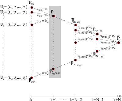
Figure 1: Switching tree: MPC with prediction horizon $N$

Now for each control sequence $U_{k}\in\mathbb{U}_{v}^{N},$ we can have a switching sequence $\sigma$ and the switched system (7) becomes an LTV system. Since $\mathbb{U}_{v}$ has $M$ number of control inputs, there will be $M^{N}$ control sequences in $\mathbb{U}_{v}^{N}$ which are shown in the switching tree in Fig. 1. For a fixed $N,\bar{P}_{N},$ the set of Riccati matrices for the switching tree will be time invariant. In the proposed MPC scheme, a receding horizon scheme with a fixed $N,\bar{P}_{N}$ is used. Therefore, in MPC the value function $V_{1}^{*}$ in the switching tree can be used as an approximation for $V_{k+1}^{*}$ and the value $V_{1}^{*}$ is characterized by the set of Riccati matrices $\mathbb{P}_{1}=\{\bar{P}_{1_{1}},\bar{P}_{1_{2}},...,\bar{P}_{1_{M^{{N}-1}}}\},$ i.e., we have

$$V_{1}^{*}(x)=\bar{x}^{T}\bar{P}_{1_{i^{*}}}\bar{x}$$ (18)

where $\bar{P}_{1_{i^{*}}}\in\mathbb{P}_{1}$ and $i^{*}=\underset{i=1,...,M^{N-1}}{arg\hskip 2.84544ptmin}\hskip 5.69046pt\bar{x}^{T}\bar{P}_{1_{i}}\bar{x}.$ In practice, computing and storing $\mathbb{P}_{1}$ will be computationally difficult for problems with larger ${N}.$ Therefore in the proposed method, we use the relaxed pruning scheme introduced [22] for reducing the size of $\mathbb{P}_{1}$ by eliminating the redundant matrices from the set. We denote $\mathbb{P}_{1\epsilon}$ as the $\epsilon-$ equivalent subset of $\mathbb{P}_{1}$ which is obtained by removing the Riccati matrices that are $\epsilon-$ redundant. We have the following definition for $\epsilon-$ redundancy:

Definition 1.

[22] For any $\epsilon\geq 0,$ a matrix $\bar{P}_{j}\in\mathbb{P}_{1}$ is called $\epsilon-$ redundant with respect to $\mathbb{P}_{1}$ if,

$$\underset{\bar{P}\in\mathbb{P}_{1}\backslash\bar{P}_{j}}{\mbox{min}}\hskip 5.69046pt\bar{x}^{T}\bar{P}\bar{x}\leq\underset{\bar{P}\in\mathbb{P}_{1}}{\mbox{min}}\hskip 5.69046pt\bar{x}^{T}\bar{P}\bar{x}+\epsilon{\parallel\bar{x}\parallel}^{2}$$ (19)

for any $\bar{x}\in\mathbb{R}^{n+1}.$

In that case we prune the matrix ${P}_{j}$ from $\mathbb{P}_{1}$ and the effect of pruning on the value function is the additional cost $\epsilon{\parallel\bar{x}\parallel}^{2}$. Next lemma [20] gives a sufficient condition for $\epsilon-$ redundancy, which is a special case of Lemma 1 in [22].

Lemma 2.

$\bar{P}_{j}\in\mathbb{P}_{1}$ is $\epsilon-$ redundant if there exists a $\bar{P}_{i}\in\mathbb{P}_{1}$ that satisfies

$$\bar{x}^{T}\bar{P}_{i}\bar{x}\leq\bar{x}^{T}\bar{P}_{j}\bar{x}+\epsilon{\parallel\bar{x}\parallel}^{2}\hskip 14.22636pt\forall\bar{x}\in\mathbb{R}^{n+1}$$ (20)

We can rewrite (20) as

$$\bar{x}^{T}[(\bar{P}_{j}+\epsilon I_{n+1})-\bar{P}_{i}]\bar{x}\geq 0\hskip 14.22636pt\forall\bar{x}\in\mathbb{R}^{n+1}$$ (21)

This can be verified using any numerical criteria for checking positive definiteness of $(\bar{P}_{j}+\epsilon I_{n+1})-\bar{P}_{i}$ and the algorithm for pruning is given in [20].

In the proposed approach we use $\mathbb{P}_{a}=\mathbb{P}_{1\epsilon}.$ This results in the approximate value function as

$$\hat{V}_{k+1}(x_{k+1})=\underset{i\in\mathbb{H}}{min}\hskip 5.69046pt\bar{x}_{k+1}^{T}\bar{P}_{i}\bar{x}_{k+1}\hskip 14.22636pt\bar{P}_{i}\in\mathbb{P}_{1\epsilon}$$ (22)

where $\mathbb{H}=\{1,2,...,\mu\},\hskip 2.84544pt\mu=|\mathbb{P}_{1\epsilon}|.$ The architecture of the proposed ADP approach and the flowchart of the offline computation are given in Fig. 2.

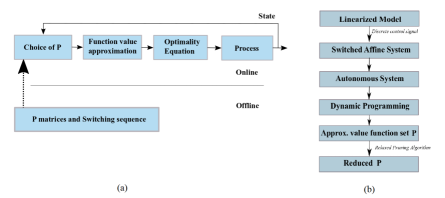
Figure 2: (a) Architecture of the proposed ADP approach (b) Flow chart of the offline Computation

4.2 Online Computation

4.2.1 ADP based MPC Scheme: Single-stage

In ADP based MPC scheme, a suboptimal control input is computed at each instant by solving

$$\hat{u}_{k}=v_{k}^{*}=\underset{v\in\mathbb{U}_{v}}{arg\hskip 2.84544ptmin}\hskip 5.69046pt[L(x_{k},v)+\hat{V}_{k+1}(x_{k+1})]$$ (23)

where $\hat{V}_{k+1}$ is the approximate value function computed using (22). Here for each control input $v\in\mathbb{U}_{v},$ we have to find the approximate value function $\hat{V}_{k+1}(x_{k+1}).$ Now $\mathbb{U}_{v}$ contains $M$ number of control inputs and to compute $\hat{V}_{k+1}$ we have to compare $\mu$ number of cost values. Therefore the online computation required for the MPC scheme is of order $\mu M.$

Algorithm 1 Online computation

  Input $x_{k}$, k, ${N}$

  for $j=1~{}to~{}M$ do

     Calculate $x_{k+1|v_{j}}$

     for $i=1~{}to~{}\mu$ do

        $V_{i}=\hat{V}_{k+1}(x_{k+1|v_{j}})$

     end for

     $V^{*}$ = min(V)

     $J_{j}=L(x_{k},v_{j})+V^{*}$

  end for

  $q$=arg min (J)

  $u_{k}=v_{q}$

  Apply $u_{k}$

  

4.2.2 ADP based MPC Scheme: Multi-stage

The control law (23) can be improved by using a multi-stage scheme, in which the control input is computed by considering additional samples around $v_{k}^{*}$ and optimizing over the samples. We denote $\mathbb{U}_{w}=\{w_{-W},...,w_{-1},w_{0},w_{1},...,w_{W}\},$ $w_{0}=0,$ which consist of $2W+1$ samples around zero. In the case of uniform sampling with a sampling interval $\varDelta u,$ we select $w_{q}=q\varDelta u,q=-W,..-1,0,1,...,W.$ Then in the second stage of optimization, the decision variable becomes $v_{k}^{*}+w$ where $w\in\mathbb{U}_{w}$ and results in the control input:

$$\hat{u}_{k}=v_{k}^{*}+w_{k}^{*}=v_{k}^{*}+\underset{w\in\mathbb{U}_{w}}{arg\hskip 2.84544ptmin}\hskip 5.69046pt[L(x_{k},v_{k}^{*}+w)+\hat{V}_{k+1}(x_{k+1})]$$ (24)

to reduce the online computation we use the same $\hat{V}_{k+1}$ (i.e., same $P$ matrix) obtained in stage 1.

5 MPC with bounded state constraints

So far we considered the MPC problem with an unconstrained state case, i.e., only the control input is constrained. In this section, we extend the ADP-based MPC scheme to nonlinear systems with both input and state constraints (bounded). We consider ${x}_{k}\in\mathbb{X},$ ${u}_{k}\in\mathbb{U},$ and $\mathbb{X},$ $\mathbb{U}$ are considered as polytopes in $\mathbb{R}^{n},\mathbb{R}^{m}$ respectively.

In the unconstrained state case we used the set of matrices $\mathbb{P}_{a}$ to approximate the value function. The set $\mathbb{P}_{a}$ is computed by pruning the set of initial matrices of the switching tree, and the pruning criteria is needed to be satisfied for all values of the state $\bar{x}.$ Now in the constrained state case we can use the set $\mathbb{P}_{a}$ and the size of $\mathbb{P}_{a}$ can be reduced further by considering the matrices that result in an optimal cost function for the states in the region $\mathbb{X},$ instead of the entire state space $\mathbb{R}^{n}.$ We define the set $\mathbb{P}_{a_{d}}$ as the set of initial matrices for the constraint state case. Then to compute $\mathbb{P}_{a_{d}},$ we discretize the constraint set $\mathbb{X}$ into $n_{\mathbb{X}}$ points and the set is denoted as $\mathbb{X}_{d}=\{x_{d_{1}},x_{d_{2}},...,x_{d_{n_{\mathbb{X}}}}\}\subset\mathbb{X}.$ Then for each ${x}_{d}\in\mathbb{X}_{d}$ we use the augmented state $\bar{x}_{d}$ to find the optimal Riccati matrix from $\mathbb{P}_{a}$ as below

$$\bar{P}^{*}=\underset{\bar{P}_{i}\in\mathbb{P}_{a}}{arg\hskip 2.84544ptmin}\hskip 5.69046pt\bar{x}_{d}^{T}\bar{P}_{i}\bar{x}_{d}\hskip 14.22636pt\bar{P}_{i}\in\mathbb{P}_{a},i\in\{1,2,...,\mu\}$$ (25)

and each time when we get a new $\bar{P}^{*}$ we add it to the set $\mathbb{P}_{a_{d}}.$ Clearly $\mathbb{P}_{a_{d}}\subseteq\mathbb{P}_{a}$ and in the constraint state case we use the set $\mathbb{P}_{a_{d}}$ for the computation of $\hat{V}_{k+1}$. Then the control input for the MPC is computed at each instant by solving

$$\hat{u}_{k}=v_{k}^{*}=\underset{v\in\mathbb{U}_{v}}{arg\hskip 2.84544ptmin}\hskip 5.69046pt[L(x_{k},v)+\hat{V}_{k+1}(x_{k+1})]$$ (26)

$$subject\hskip 2.84544ptto\hskip 5.69046ptf(x_{k},v)\in\mathbb{X}$$

The online computation can be reduced further by dividing the constraint set $\mathbb{X}$ into a finite number of polytopes $\mathbb{X}_{1},\mathbb{X}_{2},...\mathbb{X}_{z}$ and then find the set of initial matrices for each of these regions, which results in $\mathbb{P}_{a_{d_{1}}},\mathbb{P}_{a_{d_{2}}},...,\mathbb{P}_{a_{d_{z}}}.$ Then during the online computation, if $x_{k}\in\mathbb{X}_{j}$ we use the set $\mathbb{P}_{a_{d_{j}}}$ for approximating the value function. Here we have $\mathbb{P}_{a_{d_{j}}}\subseteq\mathbb{P}_{a_{d}}$ for each $j\in\{1,2,...,z\}.$ Therefore this approach can be used for reducing online computation.

6 Stability Analysis

Next, we discuss the stability of the proposed MPC scheme in which we focus on a posteriori stability analysis. In general, stability of MPC schemes is achieved by considering the optimal cost function $J_{N}^{*}(x_{k})$ as a candidate Lyapunov function. For the proposed MPC scheme (23) we obtained the cost $J_{N}^{*}(x_{k})$ as

$$J_{N}^{*}(x_{k}) =\underset{v\in\mathbb{U}_{v}}{min}\hskip 5.69046pt[L(x_{k},v)+\hat{V}_{k+1}(x_{k+1})]=L(x_{k},v^{*})+\bar{x}_{k+1}^{T}\bar{P}_{{i}^{*}}\bar{x}_{k+1}$$ (27)

$$=L(x_{k},v^{*})+\left[\begin{matrix}f(x_{k},v^{*})\\ 1\end{matrix}\right]^{T}\bar{P}_{{i}^{*}}\left[\begin{matrix}f(x_{k},v^{*})\\ 1\end{matrix}\right]$$

which is a nonlinear function of $x_{k}$ and can be non-quadratic as well because of the nonlinear mapping $f(x_{k},v^{*}).$ This complicates the stability analysis of the proposed MPC scheme since proving $J_{N}^{*}$ will be a Lyapunov function for the nonlinear system a priori will be difficult. This motivates us to go for a posteriori stability analysis [23], in which we give sufficient conditions for $J_{N}^{*}$ to be a Lyapunov function for the nonlinear system which can be verified numerically.

In the posteriori analysis, we aim to numerically show that for the proposed MPC scheme the cost $J_{N}^{*}$ will be a Lyapunov function so that the corresponding closed-loop dynamics is asymptotically stable. Before proceeding further, the following assumption is made:

Assumption 1.

The nonlinear function $f(x,u)$ is continuous and locally Lypchitz with respect to $x$ in $\mathbb{X}\times\mathbb{U},$ i.e., there exists a constant $L_{c}\in\mathbb{R}_{+}$ such that

$$\parallel f(x_{1},u)-f(x_{2},u)\parallel\leq L_{c}\parallel x_{1}-x_{2}\parallel,\hskip 14.22636pt\forall x_{1},x_{2}\in\mathbb{X},u\in\mathbb{U}.$$ (28)

Assumption 1 ensures the mapping $f(x,u)$ does not go unbounded for small changes of $x.$ Next, we analyze the stability of the nonlinear system and we had transformed the system in such a way that the origin ${x}_{k}=0$ will be the equilibrium point. We have the following theorem on stability [23]

Theorem 1.

The nonlinear system (1) with the MPC scheme is asymptotically stable on $\mathbb{X}$, if there exists a Lyapunov function $L_{f}(x_{k})$ which satisfies

$$L_{f}({x}_{k})\geq c_{1}||{x}_{k}||^{2}_{2},\hskip 14.22636pt\forall\hskip 2.84544pt{x}_{k}\in\mathbb{X}\backslash\{0\},\hskip 5.69046ptc_{1}>0,\hskip 5.69046ptL_{f}(0)=0$$ (29)

and

$$L_{f}({x}_{k+1})-L_{f}({x}_{k})\leq-c_{2}||{x}_{k}||^{2}_{2},\hskip 14.22636pt\forall\hskip 2.84544pt{x}_{k}\in\mathbb{X}\backslash\{0\},\hskip 5.69046ptc_{2}>0.$$ (30)

For the proposed MPC scheme, the value function is considered as a candidate Lyapunov function, i.e. $L_{f}(x_{k})=J_{N}^{*}(x_{k}).$ If the above conditions are satisfied for $L_{f}(x)=J_{N}^{*}(x),$ then the nonlinear system with the MPC scheme is asymptotically stable within the constrained set $\mathbb{X}$. Clearly, the first condition (29) is satisfied by $J_{N}^{*}(x_{k})$ with $c_{1}=\lambda_{min}(Q),$ since $\bar{P}_{i^{*}}\geq 0$ in (27). In order to verify the second condition, we discretize $\mathbb{X}$ into $\mathbb{X}_{d}\subset\mathbb{X}\backslash\{0\}$ and for each $x\in\mathbb{X}_{d}$ check whether $J_{N}^{*}$ satisfies the condition (30). By considering sufficiently large number of points in $\mathbb{X}_{d},$ we can find $c_{2}$ with a desired accuracy. For example if we discretize each component of the state vector with a step size $10^{-h}$ then the posteriori stability bounds computed using $\mathbb{X}_{d}$ holds up to $h$ digit precision. In order to compute $c_{2},$ for each $x\in\mathbb{X}_{d},$ we compute

$$c(x)=\frac{L_{f}\big{(}f(x,v^{*})\big{)}-L_{f}({x})}{||{x}||^{2}_{2}}=\frac{J_{N}^{*}\big{(}f(x,v^{*})\big{)}-J_{N}^{*}({x})}{||{x}||^{2}_{2}}$$ (31)

from which we obtain

$$-c_{2}=\underset{x\in\mathbb{X}_{d}}{max}\hskip 5.69046ptc(x).$$ (32)

Now, if $-c_{2}<0$ (i.e., $c_{2}>0$), then $J_{N}^{*}$ satisfies (30) and can be used as a Lyapunov function for the nonlinear system with the MPC scheme.

7 Experimental study: Multi-Tank System

Figure 3(a) shows the block diagram of the multi-tank system and 3(b) shows the actual experimental setup. Our target is to maintain the water levels of the three tanks at the desired values. In the computer, we specify the set point and load the control algorithm. The water levels $H_{1}$,$H_{2}$, and $H_{3}$ are controlled either by controlling the valve or by controlling the speed of the motor. In this paper, we keep the valve position fixed and give the control signal to vary the speed of the motor that pumps water to the tank. The differential pressure sensor measures the water level and sends it back to the computer through the data acquisition system.

In the multi-tank system, we pump the water to the top tank from the reservoir located at the bottom. The liquid inflow $q$ is controlled by the pump. The valve $C_{1}$ restricts the flow of the liquid from the topmost tank to the intermediate tank. The water flows down due to gravity from the second tank to the third tank passing through valve $C_{2}$. And the liquid finally reaches the reservoir through valve $C_{3}$. The computer communicates with the level sensors, pumps, and valves by a dedicated input-output board and power interface [21]. A real-time software operating in MATLAB Real-Time Windows Target (RTWT) rapid prototyping environment controls the input-output board. The MATLAB version on the computer is R2018b and Intel Core i7 processor at 3GHz with 32GB RAM. The run time of the experiment is 250 sec with a sampling time of 0.01 sec.

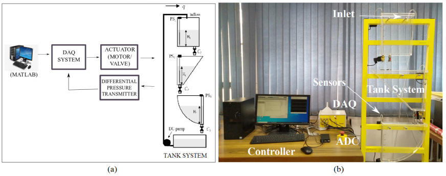
Figure 3: Multi-Tank Control System (a) Block diagram (b) Experimental setup

7.1 System Equations

Bernoulli’s law governs the outflow rate of the fluid from a tank. The outflow rate of a tank is given by:

$$Q_{r}=f_{0}S\sqrt{2gH_{0}}$$ (33)

where $f_{0}$ is orifice outflow coefficient and S is the output area of orifice.
The nonlinear model of the multi-tank system [21] is given by:

$$\frac{dH_{1}}{dt} =\frac{1}{\beta_{1}(H_{1})}q-\frac{1}{\beta_{1}(H_{1})}C_{1}H_{1}^{\alpha_{1}}$$ (34)

$$\frac{dH_{2}}{dt} =\frac{1}{\beta_{2}(H_{2})}C_{1}H_{1}^{\alpha_{1}}-\frac{1}{\beta_{2}(H_{2})}C_{2}H_{2}^{\alpha_{2}}$$ (35)

$$\frac{dH_{3}}{dt} =\frac{1}{\beta_{3}(H_{3})}C_{2}H_{2}^{\alpha_{2}}-\frac{1}{\beta_{3}(H_{3})}C_{3}H_{3}^{\alpha_{3}}$$ (36)

where height of fluid, resistance of output orifice, flow coefficients are $H_{i}$, $C_{i}$, $\alpha_{i}$ respectively for $i-{th}$ tank, $i=1,2,3$. The parameter values are given in the next section.
$\beta_{1}(H_{1})=aw_{t}$ - Cross sectional area of topmost tank; $\beta_{2}(H_{2})=cw_{t}+\frac{H_{2}}{H_{2max}}bw_{t}$ - Cross sectional area of intermediate tank; $\beta_{3}(H_{3})=w_{t}\sqrt{R^{2}-(R-H_{3})^{2}}$ - Cross sectional area of bottom tank. The variable cross-section of the tanks, the contribution of valve geometry & flow dynamics, and the pump & valve input-output characteristics are the potential factors that challenge the control design.

7.2 Model and Parameters

The linearized dynamical model of the three-tank system, linearized around ($H_{10},H_{20},H_{30}$), is described as: $h_{k+1}=Ah_{k}+Bu_{k}$

$$A=\begin{bmatrix}\frac{-C_{1}\alpha_{1}}{aw_{t}H_{10}^{1-\alpha_{1}}}&0&0\\ \frac{C_{1}\alpha_{1}}{w_{t}\bigg{(}c+b\frac{H_{2}0}{H_{2max}}\bigg{)}H_{10}^{1-\alpha_{1}}}&\frac{-C_{2}\alpha_{2}}{w_{t}\bigg{(}c+b\frac{H_{2}0}{H_{2max}}\bigg{)}H_{20}^{1-\alpha_{2}}}&0\\ 0&\frac{C_{2}\alpha_{2}}{w_{t}\sqrt{R^{2}-(H_{3max}-H_{3}0)^{2}}H_{20}^{1-\alpha_{2}}}&\frac{-C_{3}\alpha_{3}}{w_{t}\sqrt{R^{2}-(H_{3max}-H_{3}0)^{2}}H_{30}^{1-\alpha_{3}}}\end{bmatrix},\hskip 2.84544ptB=\begin{bmatrix}\frac{1}{aw_{t}}\\ 0\\ 0\end{bmatrix}$$ (37)

The experimental setup uses the parameter values $H_{1max},H_{2max},H_{3max}$ = 0.35 m, $a$ = 0.25 m, $b$ = 0.345 m, $w_{t}$ = 0.035 m, $c$ = 0.10 m, $R$ = 0.365 m. The constraints are the maximum height of the tank is 0.35 m and the control input could be varied from 0.54 to 1 volt corresponding to the minimum and the maximum motor speed respectively.We discrete (quantized) set of control inputs into $\mathbb{U}_{v}=\{v_{1},v_{2},...,v_{6}\}$ and $\mathbb{U}_{v}\subset\mathbb{U}.$ The LTI system with discrete set of controls $\mathbb{U}_{v}$ is represented as a switched affine system as in (6) with $M=6$ subsystems.

7.3 Results

We have implemented algorithm 1 in the setup. Figure 4(a) shows the responses of single-stage ADP (ADP-1) when applied to the multi-tank system. The corresponding control signal is shown in figure 4(b). We observe continuous chattering of the control signal due to the disturbance in state measurement.

A more accurate control at each instant is obtained by the use of multi-stage ADP (ADP-2). The evolution of states for multi-stage ADP applied to the multi-tank system is shown in figure 5(a). And the corresponding control signal is shown in figure 5(b). We notice that the control signal in figure 5(b) has become more smooth compared to figure 4(b).

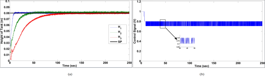
Figure 4: Single-stage ADP (a) Evolution of states (b) Control signal

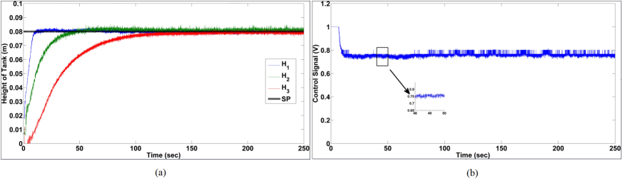
Figure 5: Multi-stage ADP (a) Evolution of states (b) Control signal

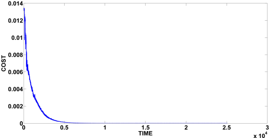
Figure 6: Value of Cost function along closed loop trajectory

By carrying out a posteriori analysis, we observed that the proposed controller leads to asymptotical stability. For the proposed MPC, we have obtained $c_{2}=0.4318$ for the Lyapunov function $L_{f}(x_{k})=J_{N}^{*}(x_{k}).$ This is obtained by discretizing the constraint set $\mathbb{X}$ in to $\mathbb{X}_{d}$ which contains $10^{9}$ points (step size $10^{-3}$, i.e. $h=3$) and computing $c(x)$ as in (31) for each $x\in\mathbb{X}_{d}.$ From which the maximum value gives $c_{2}$ and for the multi-tank system with proposed MPC scheme we obtained $c_{2}=0.4318>0$. Consequently, the cost $J_{N}^{*}(x_{k})$ becomes a Lyapunov function and the proposed MPC scheme results in asymptotically stable closed loop dynamics with $3$ digit precision as per Theorem 1. From Fig. 6, we can see that the value function is decreasing along the trajectory. We observe that the performance function reduces to zero as the states reach the equilibrium point.

7.4 Comparison

The comparison of the computation time is shown in table 1. The computation of Nonlinear Model Predictive Control (NMPC) is more (27%) compared to ADP-based MPC. ADP-1 is the single-stage Approximated Dynamic Programming based MPC and ADP-2 is the multi-stage ADP based MPC. The computation time of ADP-2 is slightly higher (0.39%) compared to ADP-1 due to the additional computation time taken for the second stage of iteration to find a more suitable control signal. But in multi-stage ADP we get smoother control compared to a single-stage as observed from 4(b) and 5(b). The ADP-3 shows the case where we considered the state constraints. The computation time got further reduced as we were able to reduce the set of P matrices. The table 1 also shows the comparison of Integral Square Error (ISE=${\sum_{k=0}^{T}}{||e_{k}||}_{2}^{2}$; where $e_{k}=x_{k}-x_{r}$ ) for different strategies. The value is least for NMPC, but the proposed strategies have comparable performance compared to NMPC.

Table 1: Comparison of Different Strategies

Control Scheme	Time (sec)	ISE
NMPC	0.0012	10.3225
ADP-1	$4.2810\times 10^{-5}$	12.3790
ADP-2	$7.0993\times 10^{-5}$	11.5444
ADP-3	$9.1070\times 10^{-6}$	13.2071

8 Conclusion

In this paper, we have proposed an approximate dynamic programming-based MPC to reduce the online computation time. To evaluate the advantage of the proposed schemes they were applied to a multi-tank nonlinear system. A smoother control was obtained in the multi-stage MPC scheme compared to the single-stage MPC scheme. The computation time was further reduced by considering state bounds. The method reduces the computation time significantly, while the performance in terms of ISE is comparable.

References

- [1] K. Basil, C. Mark, “Model Predictive Control- Classical, Robust and Stochastic”, Springer, 2015.
- [2] J. M. Lee and J. H. Lee, “Approximate dynamic programming-based approaches for input–output data-driven control of nonlinear processes”, Automatica, vol. 41, pp. 1281-1288, 2005.
- [3] F. Lewis and D. Liu, “Reinforcement Learning and Approximate Dynamic Programming for Feedback Control”, John Wiley and Sons, 2012.
- [4] P. Rokhforoz, H Kebriaei, and M. Ahmadabadi,“Large scale dynamic system optimization using dual decomposition method with approximate dynamic programming,” Systems and Control Letters, vol. 150, pp. 550-565, 2021.
- [5] A. Keyser, H. Vansompel, and G. Crevecoeuri,“Real-Time Energy-Efficient Actuation of Induction Motor Drives Using Approximate Dynamic Programming,” IEEE Transactions on Industrial Electronics, vol. 68, 2021.
- [6] J. M. Lee and J. H. Lee, “Approximate Dynamic Programming Strategies and Their Applicability for Process Control: A Review and Future Directions”, International Journal of Control, Automation, and Systems, vol. 3, pp. 263-278, 2004.
- [7] L. Dong, J. Yan, X. Yuan, H. He, and C. Sun, “Functional Nonlinear Model Predictive Control Based on Adaptive Dynamic Programming”, IEEE Transactions On Cybernetics, vol. 49, pp. 23-35, 2019.
- [8] N. Zhang, B. Leibowicz, and G. Hanasusanto, “Optimal Residential Battery Storage Operations Using Robust Data-Driven Dynamic Programming”, IEEE Transactions on Smart Grid, vol. 11, pp. 1771-1780, 2020.
- [9] M. Park, K. Kalyanam, S. Darbha, P. Khargonekar, M. Pachter, and P. Chandler, “Optimal Residential Battery Storage Operations Using Robust Data-Driven Dynamic Programming”, IEEE Transactions on Automation Science and Engineering, vol. 13, pp. 564-578, 2016.
- [10] T. Sun and X. Sun, “Adaptive Dynamic Programming Scheme for Nonlinear Optimal Control With Unknown Dynamics and Its Application to Turbofan Engines”, IEEE Transactions on Industrial Informatics", vol. 17, pp. 367-376, 2021.
- [11] B. Luo, D. Liu, T. Huang, and J. Liu, “Tracking Control Based on Adaptive Dynamic Programming With Multistep Policy Evaluation”, IEEE Transactions on Systems, Man, and Cybernetics: Systems, vol. 49, pp. 2155-2165, 2019.
- [12] X. Xu, C. Lian, L. Zuo, and H. He, “Kernel-Based Approximate Dynamic Programming for Real-Time Online Learning Control: An Experimental Study”, IEEE Transactions on Systems, Man, and Cybernetics: Systems, vol. 22, pp. 146-156, 2014.
- [13] H. Zhang, H. Su, K. Zhang, and Y. Luo, “Event-Triggered Adaptive Dynamic Programming for Non-Zero-Sum Games of Unknown Nonlinear Systems via Generalized Fuzzy Hyperbolic Models”, IEEE Transactions on Fuzzy Systems, vol. 27, pp. 2202-2214, 2019.
- [14] D. Bertsekas, “Dynamic Programming and Optimal Control”, IEEE Transactions on Fuzzy Systems, Athena Scientific, 2005.
- [15] D. Bertsekas, “Dynamic Programming and Optimal Control, Vol II: Approximate Dynamic Programming”, Athena Scientific, 2012.
- [16] L. Grune and J. Pannek “Nonlinear Model Predictive Control Theory and Algorithms”, Springer, 2011.
- [17] J. Liu, D. Pena, and P. Christofides, “Distributed Model Predictive Control of Nonlinear Process Systems”, AIChE Journal, vol. 55, pp. 1171-1184, 2009.
- [18] M. Maiworm, D. Limon, and R. Findeisen, “Online learning-based model predictive control with Gaussian process models and stability guarantees”, International Journal of Robust and Nonlinear Control, vol. 31, pp. 8785-8812, 2020.
- [19] M. Augustine and D. Patil, “A Practically Stabilizing Model Predictive Control Scheme for Switched Affine Systems,” IEEE Control System Letters, vol. 7, pp. 625-630, Sep. 2022.
- [20] M. Augustine and D. Patil, “A Computationally efficient LQR based Model Predictive Control Scheme for Discrete-time Switched Linear Systems,”, IEEE Conference on Decision and Control, Texas, USA, Dec. 2021
- [21] Inteco, “Multi-Tank User Manual,” Inteco Ltd, Krakow, 2003.
- [22] W. Zhang, J. Hu and A. Abate,“Infinite-Horizon Switched LQR Problems in Discrete Time: A Suboptimal Algorithm With Performance Analysis,” IEEE Transactions on Automatic Control, vol. 57, no. 7, pp. 1815-1821, Jul. 2012.
- [23] T. Geyer, G. Papafotiou, and M. Morari,“Hybrid model predictive control of the step-down dc-dc converter,” IEEE Transactions on Control Systems Technology, vol. 16, pp. 1112-1124, Nov. 2008.
- [24] A. Forootani, R. Iervolino, M. Tipaldi, and J. Neilson,“Approximate Dynamic Programming for Stochastic Resource Allocation Problems,” IEEE/CAA Journal of Automatica Sinica, vol. 7, pp. 975-990, 2020.
- [25] P. Beuchat, J. Warrington, and J. Lygeros,“Point Wise Maximum Approach to Approximate Dynamic Programming,” IEEE Transactions on Automatic Control, vol. 67, pp. 251-266, 2022.
- [26] K. Chacko, S. Janardhanan, and I. Kar,“Computationally Efficient Nonlinear MPC for Discrete System with Disturbances,” International Journal of Control, Automation and Systems, vol. 15, 2022.
- [27] K. Chacko, S. Janardhanan, and I. Kar,“Efficient Nonlinear Model Predictive Control for Discrete System with Disturbances,” Int. Conf. on Control, Automation, Robotics and Vision, Singapore, 2018.
- [28] S. Huang, Z. Hu, G. Cao, G Jing, and Y. Liu,“Input-Constrained-Nonlinear-Dynamic-Model-Based Predictive Position Control of Planar Motors,” IEEE Transactions on Industrial Electronics, vol. 68, pp. 50-60, 2021.