Dealer Strategies in Agent-Based Models

Abstract

This paper explores the utility of agent-based simulations in realistically modelling market structures and sheds light on the nuances of optimal dealer strategies. It underscores the contrast between conclusions drawn from probabilistic modelling and agent-based simulations, but also highlights the importance of employing a realistic test bed to analyse intricate dynamics. This is achieved by extending the agent-based model for auction markets by Chiarella et al. (2008) to include liquidity providers. By constantly and passively quoting, the dealers influence their own wealth but also have ramifications on the market as a whole and the other participating agents. Through synthetic market simulations, the optimal behaviour of different dealer strategies and their consequences on market dynamics are examined. The analysis reveals that dealers exhibiting greater risk aversion tend to yield better performance outcomes. The choice of quote sizes by dealers is strategy-dependent: one strategy demonstrates enhanced performance with larger quote sizes, whereas the other strategy show a better results with smaller ones. Increasing quote size shows positive influence on the market in terms of volatility and kurtosis with both dealer strategies. However, the impact stemming from larger risk aversion is mixed. While one of the dealer strategies shows no discernible effect, the other strategy results in mixed outcomes, encompassing both positive and negative effects.

JEL classification: C63, G15, D80.

Keywords: agent-based model, limit orderbook, market maker, liquidity provider.

1 Introduction

This paper develops an agent-based model centred around a limit orderbook (hereafter LOB) as a mainstay for information dissemination among market participants, facilitating opinion formation and subsequent price discovery. It emphasises the introduction of a passive dealer who acts as a liquidity provider. In contemporary financial markets, auctions are the prevailing operational mode, where buyers and sellers simultaneously set their quotes. This results in complex dynamics that have yet to be understood from both a behavioural finance and economic perspective. In the subsequent sections, the model will be used as a test bed to analyse the dealer’s optimal behaviour but also the impact on market dynamics.

The presented work is primarily concerned with the introduction of a liquidity provider which is an essential part of financial markets. The impact of such agents has garnered attention from various perspectives. While numerous studies suggest that high frequency trading can disrupt price discovery, increase volatility beyond fundamentals, there is an equal body of research asserting that liquidity has expanded, as measured by increased order book depth and size. Additionally, spreads have significantly narrowed resulting in less room for manipulation and predatory strategies. Given the complexity of financial markets and growing influence of computer-driven traders, it is important to further investigate the influence of liquidity providers.

This work primarily relates to Vuorenmaa and Wang (2014) where the authors utilise the classical agent-based model developed in Chiarella and Iori (2002) and Chiarella et al. (2008). Vuorenmaa and Wang’s (2014) goal is to study high frequency traders (HFT; throughout the paper, also referred to as dealer) more realistically in situations of flash crashes. As in Avellaneda and Stoikov (2008), HFTs optimise their inventory risk while providing continuous liquidity. The study incorporates an institutional trader who is able to initiate a flash crash through specific types of selling strategies. They find that the probability of a flash crash increases with more HFT agents or smaller inventory size. Market volatility is negatively correlated with the aforementioned factors and deriving optimality conditions without knowledge of the decision maker’s preferences is unfeasible.

This model builds upon previous work of Chiarella and Iori (2002) and Chiarella et al. (2008). The papers introduce an order-driven market with multiple types of representative agents including fundamentalists, chartists and noise traders. The later extension of Chiarella et al. (2008) allows agents to submit orders by maximising their expected utility and apply varying time horizons for different types of strategies. In addition, a passive liquidity provider is introduced to the model following Avellaneda and Stoikov (2008) where a strategy is developed for stock dealers who provide liquidity in a LOB. The authors combine the utility framework of Ho and Stoll (1981) with results of microstructure literature on the limit orderbook. Following a two-step procedure the dealer determines an indifference price for a given asset by taking his inventory position as well as risk aversion into account. Afterwards, bid-ask quotes are derived from the probability of order arrivals and risk aversion.

The aim of this work is to contribute to the literature on financial agent-based models of auction markets and the research on optimal dealer quoting. In particular I will contribute with a detailed study of the wealth implications and price discovery driven by dealer behaviour.

The first part serves as a prelude to subsequent topics concerning the main model and addresses the necessity of agent-based models by critically examining probabilistic simulations as in Avellaneda and Stoikov (2008). Subsequently, I integrate a risk-averse dealer in a LOB framework enabling a more realistic modelling of price discovery and feedback loops. The study will analyse two distinct dealer strategies: 1) An agent that optimises profits and inventory risk akin to Avellaneda and Stoikov (2008) and 2) a dealer resembling the approach in Fushimi and González Rojas (2018) who uses a practitioners rule to manage inventory risk. Furthermore, I compare the strategies with a naive liquidity provider who simply provides fixed volume around the mid-price. Other agent types deployed choose their allocation in the risky instrument by maximising their utility under constant relative risk aversion. While this extension adds complications to the simulation by introducing wealth-dependent allocations, it enables a realistic assessment of the feedback loop between an agent’s wealth and different parameter sensitivities.

My second contribution is to shed light on the influence of preference parameters on the dealer’s optimal behaviour. For this purpose, several parameters in the behavioural function of the dealer have to be calibrated in order to create realistic dynamics. Establishing a baseline parameter set is crucial as it ensures the dealer’s profitability which is her primary motivation. Moreover, I present the endogenous feedback loop and its implications for price changes and wealth. By choosing parameter values the dealer influences the market dynamics which the dealer and other agents then react to in turn. Conclusions on the optimal behaviour of the dealer will be derived along with the implications on the market. Given the dealer’s decisions are entangled with price dynamics but also personal wealth, it is important to clearly present dependencies.

The findings underscore the importance of agent-based simulations as a valuable tool for achieving more realistic market-like structures. It is shown that conclusions on the dealer strategy under probabilistic modelling may be contradictory to agent-based simulations. Further, several critical features such as time dependent effects of inventory and its management cannot be analysed in full depth without a realistic test bed. The study explores sensitivities with respect to the dealer’s preferences to understand their impact on both the dealer’s wealth and market dynamics. An increase in the dealer’s risk aversion is found to elevate market volatility while reducing kurtosis of market returns. Overall dealers gain more wealth by operating more risk averse. Adjusting the dealer’s maximum order size leads to opposing outcomes as the optimising dealer benefits through capitalising on larger trades while the other experiences constant wealth loss. Markets clearly favour larger quote size as visible in decreased volatility and kurtosis. Stylised agents, in particular fundamentalists and chartists, augment their wealth gains as max. order size increases. Decreasing the dealer’s sensitivity to her inventory will lead to a less abrupt downward adjustment of quoted volume and shows a positive impact on her wealth. Similarly market return variance and kurtosis are dampened as order size is adjusted less drastically.

The paper is organised as follows: Section 2 provides an overview of the literature. In particular the models most closely related to this work will be discussed. Section 3 continues by demonstrating the difficulties and limits of a theoretical and probabilistic evaluation of the market maker’s optimal quoting rule. In section 4, the main model is described and linked to the original literature presented earlier. Finally, section 5 presents the results and section 6 concludes.

2 Literature Review

Agent-based models have gained increasing attention over the last decades. Much of economics research condense human behaviour into structural models with (boundedly) rational agents aiming to characterise features in an easily interpretable way. The findings in the area of behavioural finance have supported the approach which is taken by agent-based financial markets research. Using a simulation environment in which individual behaviour is explicitly defined and agents interact with each other, sophisticated macro features can be generated that replicate facts of financial markets. This part will serve as an introduction into the topic, highlighting the, for this work, important contributions. Note that the review is rather exhaustive which is required to have the background for the model deployed in the main part. Models designed by Chiarella and Iori (2002) and Chiarella et al. (2008) are the foundation for the work presented here. The authors studied how different trading strategies affect price discovery in an order driven market as well as the effect of market design features on liquidity.

Like the majority of real world trading, the model centres around a so called limit orderbook which serves as a platform for price discovery. The LOB takes all incoming orders, stores them as decreasing/increasing sequence for buy/sell orders in price-time priority, and finally matches buyers and sellers when bids and asks cross. In their model, agents decide sequentially about sending orders which have a finite lifetime $\tau$. A simple mechanism is put in place to remove the oldest $\tau$ orders: at every timestamp $t$, $\nu$ is drawn from a uniform distribution, if $\nu<\omega$, a constant, the oldest $\tau$ orders are cleared. The platform determines the price at timestamp $t$ as the last transaction price in case a transaction occurred, otherwise it is calculated as $p_{t}=(p_{t}^{bid,best}+p_{t}^{ask,best})/2$. If no bids (asks) are present, then the previous price is used. In this model prices are generally positive and can take only pre-specified values on a grid determined by the tick size $\Delta$.

Chiarella and Iori (2002) assume a representative agent that combines fundamentalist, chartist and noise trader behaviour to forecast returns denoted with $\hat{r}$

$$\hat{r}^{i}_{t,t+\tau}=g^{i}_{1}\frac{(p^{f}-p_{t})}{p_{t}}+g^{i}_{2}\bar{r}_{L^{i}}+n_{i}\epsilon_{t}$$ (1)

where $g^{i}_{1}>0$, $g^{i}_{2}$ and $n_{i}$ are weights assigned to fundamentalists, chartists and noise traders respectively. The latter have zero intelligence, thus base their prediction on a Gaussian random variable, $\epsilon_{t}$. The fundamental price, $p^{f}$, is only known to fundamentalists, upon which they base their trading decision. In particular, they want to buy (sell) the security if the market price is below (above) the fundamental price. Chartists extrapolate recent trends and, hence, base their decision on past returns, $\bar{r}_{L^{i}}$, calculated as the average return over the interval $L^{i}$ sampled from a uniform distribution $\mathcal{U}(0,L^{max})$

$$\bar{r}_{L^{i}}=\frac{1}{L^{i}}\sum_{j=1}^{L^{i}}ln\frac{p_{t-j}}{p_{t-j-1}}\text{.}$$ (2)

At every timestamp $t$, an agent is chosen to submit an order with a price to the LOB which is determined as $\hat{p}_{t+\tau}^{i}=p_{t}\exp(\hat{r}^{i}_{t+\tau})$. If the agent forecasts a price increase she decides to buy a unit of the stock and vice versa. It is implicitly assumed in this formulation that the agents know the price history as well as the prevailing fundamental price.

In their findings, the authors conclude that all three types of agents are necessary to create realistic return dynamics: the chartist reaction function generates large price jumps and clustering of volatility while fundamentalists tend to reduce the excursions away from the fundamental price. Chartists reinforce the clustering as they experience higher submission rates of matched orders in more volatile markets. Similarly the bid-ask spread is correlated with trading volume as the LOB is increasingly depleted around the mid-price.

Chiarella et al. (2008) extend the original version to allow agents to submit orders by maximising their expected utility and apply varying time horizons for the different types of strategies. Specifically, agents are assumed to maximise their utility of wealth, $u$, under constant absolute relative risk aversion (hereafter, CARA)

$$\operatorname*{max}_{Z^{i}_{t+\tau}}\mathbb{E}\left[u(W^{i}_{t+\tau},\gamma^{i})\right]$$ (3)

$$u(W,\gamma)=-e^{-\gamma^{i}W^{i}_{t+\tau}}$$ (4)

where $\gamma$ is the risk aversion of agent $i$. The wealth, $W$, of each agent at timestamp $t$ is defined as the sum of the market value of their individual stock portfolio and cash

$$W_{t}^{i}=q_{t}^{i}p_{t}+C_{t}^{i}$$ (5)

where $q_{t}^{i}\geq 0$ and $C_{t}^{i}\geq 0$ are respectively stock and cash positions. As implied by the inequalities, short-selling is not permitted. Given the CARA utility defined above, the agents can calculate their optimal allocation, $Z$, towards the risky asset by

$$Z_{t}^{i}=\frac{ln(\hat{p}_{t+\tau}^{i}/p_{t})}{\gamma^{i}{\sigma_{t}^{2}}W^{i}_{t}}$$ (6)

where the actual investment made is independent of the individual wealth as $W^{i}_{t}$ is cancelled out. The market volatility is denoted by $\sigma^{2}$.

In this extended model, the authors provide evidence that a significant chartists component is needed to emphasise trends and create jumps, which are typical of real financial markets. Further it is shown that all types of agents are required to create a realistic shape of the LOB: fundamentalists reduce the imbalance between buy/sell orders stemming from noise trader behaviour and chartists widen the distribution away from mid-prices.

A strand of the operations research literature is concerned with defining optimal rules on how dealers should place their quotes conditional on a set of objectives. Avellaneda and Stoikov (2008) define the problem in terms of an expected utility framework where the dealer optimises her inventory through setting bid-ask quotes under uncertainty from the transaction risk caused by the stochastic movement of the stock price and arrival rate of orders. The stock price is assumed to evolve according to a Brownian Motion without drift while the arrival of orders is modelled as a Poisson intensity.

A two step process is derived where the dealer first estimates a reservation price, $p_{t}^{r}$, making her indifferent to trade

$$p_{t}^{r}=p_{t}-q_{t}\gamma\sigma^{2}_{t}(T-t)$$ (7)

where $q_{t}$ is the dealer’s inventory at timestamp $t$, $\gamma$ defines her risk aversion and $\sigma^{2}_{t}$ is the variance of market returns. The reservation price is the difference between the current price and the inventory adjusted for risk aversion and variance. Hence, the reservation price is tilted away from the inventory side. In the subsequent step, the bid-ask spread, $\delta^{a}+\delta^{b}$, is computed around the reservation price

$$\delta^{a}+\delta^{b}=\gamma\sigma^{2}_{t}(T-t)+\frac{2}{\gamma}ln(1+\frac{\gamma}{\kappa})$$ (8)

where $\kappa$ is the arrival intensity. As the intensity of order arrivals rises, dealers are willing to trade more frequently. Simultaneously, they reduce the spread, thereby decreasing the likelihood of holding an unbalanced inventory. Likewise the spread increases in risk aversion and variance, but is reduced closer to session end. The latter is used by the dealer to increase the probability to end the day flat in terms of her inventory and is reflected in the term $T-t$ with $T$ referring to the session’s closing time. Probabilistic simulations were performed which show that the optimal strategy has a lower variance in the P&L profile and final inventory compared to a naive benchmark strategy.

After the flash crash of 2010, academics began to investigate the impact of high-frequency traders on market stability. Vuorenmaa and Wang (2014) combine the work by Chiarella et al. (2008) and Avellaneda and Stoikov (2008) described above to model HFT agents more realistically in situations of flash crashes. The authors introduce an institutional investor who uses an execution algorithm which follows a selling strategy that triggers a flash crash. They find that the probability of a flash crash rises with an increasing number of HFT agents or tighter inventory control. Contrary, market volatility will decrease with higher number of HFT agents. It was noted that setting variables optimally is not possible without knowing the preferences of the regulator/decision maker.

The here presented work will build on the models developed in the above-described contributions. In particular I am going to unite agent-based models from economics literature and theoretical results from operations research of optimising dealers to derive insights in an simulation environment.

3 Inventory Risk in Liquidity Provision Strategies

This section will review the baseline Avellaneda and Stoikov (2008) model (AS model, dealer or strategy) and demonstrate shortcomings when considering large order sizes or inventory risks. Further, this part deals as a prologue to the model derived in the next section by emphasising the importance of agent-based simulations.

The AS model is simulated by iterating through time $T$ in $dt$ increments. At every timestamp $t$, the dealer computes bid and ask prices according to equation (8) based on the prevailing market price and her inventory. At the next timestamp, $t+dt$, the market price is updated by a random increment of $\pm\sigma\sqrt{dt}$. With a probability of $\lambda^{a}(\delta^{a})dt$ the dealer’s inventory decreases by one unit while her cash increases by $p_{t}+\delta^{a}$. Conversely, with a probability of $\lambda^{b}(\delta^{b})dt$ the inventory increases by one unit while cash decreases by $p_{t}-\delta^{b}$. The probabilities $\lambda^{a}(\delta^{a})$ and $\lambda^{b}(\delta^{b})$ denote the execution intensity of the dealer’s orders where each single term stands for the arrival of buy and sell orders respectively. Thus, a change in wealth is determined as the difference between execution price, derived from equations (7) and (8), and the prevailing market price, which follows a Brownian Motion. Figure 3 displays the distribution of terminal wealth.

Notably, the AS model is a probabilistic simulation where a single unit of the underlying is traded and the market price is independent from the actual trading - both assumptions are not realistic. To demonstrate the issue of simplification to an unitary order size, the simulation is adjusted by introducing a random variable $x_{t}$ drawn from a Gamma distribution, specifically $\Gamma(\alpha=2,\beta=15)$. At every timestamp $t$ where the dealer makes a transaction, $x_{t}$ determines the trade size; inventory as well as wealth are adjusted incorporating the random size.

Figure 3 illustrates profit distributions for a range of strategies. The AS model is simulated following their work with a unitary order size. Additionally, the profit distribution of the adjusted AS model is shown when order size varies randomly, as described above. To draw a meaningful comparison a naive dealer strategy is created. The naive strategy quotes a constant order size of $\phi_{t}^{max}=15$ around the market price. To support the underlying thesis, the spread is calculated the same way as in the AS model in equation (8).

The terminal profit distribution clearly shows a profit decrease with the adjusted AS strategy as mean profits are visibly shifted to the left. This is a consequence of a larger inventory and thus a greater effect on wealth from market price fluctations. In contrast, the baseline strategy with unitary order sizes maintains a low inventory and as such allows the bid-ask spread revenue to largely neutralize the impact of price fluctuations. However, this compensatory mechanism is absent in the adjusted AS strategy. Counter to what would be expected, the naive strategy significantly outperforms the AS dealer. The reason can be found in the adjustment of the reference price. The naive dealer uses a symmetric quote around the mid-price. This earns her a higher compensation from the bid-ask spread than the AS dealer who shifts her reservation price toward the inventory side, thereby losing out on potential profit.

In practice, risk managers often introduce value-at-risk limits which, simply put, translates into inventory size limits. To show how the wealth is impacted by a risk management rule, an inventory adjustment from Fushimi and González Rojas (2018) is used (hereafter referred to IR model, dealer or strategy). The authors extend the AS model by introducing a dynamic order sizing framework to rule out excessive inventory by placing smaller order sizes in the direction of the excess inventory

$$\phi_{t}^{bid}=\begin{cases}\phi_{t}^{bid,max}&\text{if }q_{t}\leq 0\\ \phi_{t}^{bid,max}e^{\eta^{bid}q_{t}}&\text{if }q_{t}>0\\ \end{cases}$$ (9)

$$\phi_{t}^{ask}=\begin{cases}\phi_{t}^{ask,max}&\text{if }q_{t}\geq 0\\ \phi_{t}^{ask,max}e^{-\eta^{ask}q_{t}}&\text{if }q_{t}<0\\ \end{cases}$$ (10)

where $\phi_{t}^{ask,max}$ and $\phi_{t}^{bid,max}$ are the maximum ask and bid order sizes the dealer is willing to quote at any point in time, $\eta^{ask}$ and $\eta^{bid}$ are the adjustment factors (also called inventory skew) that will decrease the quote size as soon as the inventory is different from zero. Simulating this strategy like the previous examples, a similarly good performance as with the naive strategy can be achieved. The higher mean is attributable to a larger quote size at the reversing transaction and, thus, greater compensation through the bid-ask spread while lower variance is due to a more constrained inventory position.

Fig. 1.: Terminal wealth distributions for the AS model with unitary (light grey) and random order size (light blue) as well as the IR strategy (blue) taking the inventory adjustment of Fushimi and González Rojas (2018) into account. For a complete comparison a naive strategy (dark blue) is included. The histograms contain 1000 simulation runs which are based on the same parameter space as in Avellaneda and Stoikov (2008) if not stated differently.

To motivate the subsequent part of this work, these examples highlight the general need for having deeper analysis within a simulation framework. The profit distribution in Figure 3 raises the obvious question why a naive strategy outperforms an optimised model. A simple rule based stock management shows superior profits. The absence of a realistic simulation platform renders it impractical to analyze the underlying behavior, especially when trying to determine the causes of specific instances of under-/overperformance. Most notably, the dealer impact on market dynamics remains unexplained. An accumulation of inventory was eliminated in the simulations as the probabilities will eventually be high enough so that a reverse transaction will take place pulling the inventory towards zero. Unfortunately, real markets do not strictly following any well known distribution; as such mean reverting behaviour to the zero inventory is not granted. In fact, without restricting the dealer, she may accumulate vast amounts of stocks. By introducing the inventory rule, the impact on price discovery is seemingly different. Take a situation where the dealer’s inventory is saturated so that she removes one side of the quote. Considering the LOB’s depth and the distance between orders, the calculated mid-price may experience jumps. Similarly, the AS dealer will set her quotes around an reservation price which can tilt the market price in a particular direction. These effects will move through the market by means of feedback loops with the other participants and eventually lead to a different price path. Further, the AS strategy assumes that the market returns follow a Brownian motion. However, prices may experience trends and perpetuating behaviour in real markets. To account for endogenous effects, market participants and their interactions have to be modelled explicitly. To understand these time-dependent effects enforced by inventory risk management and dynamic interaction, the need for an agent-based model is bolstered.

4 The Model

I introduce a new model that improves on the results shown in the previous section. It is suitable as a test-bed to analyse optimal behaviour of the dealer and agents and can outline market reactions. In the following I will describe the different components of the model including the assets traded, agents who interact with each other through a limit orderbook and the simulation procedure.

4.1 Assets

For simplicity, assume a single tradable asset in the form of an arbitrary stock. The price of the stock is determined through the interaction of the different agents via a LOB. Furthermore, agents exchange cash and stock in their individual transactions. Cash is assumed to carry zero interest and to have a constant currency value. While the stock price is determined by agent interactions, fundamental type agents (described below) are said to know the fundamental value $p^{f}$ of the asset. The value is determined at every timestamp $t$ and assumed to follow a random process which causes jumps and subsequently leads to readjustment of the agent behaviour

$$p_{t}^{f}=\begin{cases}p_{t-1}^{f}(1+j)&\text{if }u_{t}<\iota\\ p_{t-1}^{f}&\text{otherwise}\\ \end{cases}$$ (11)

where $j$ is an information adjustment constant by which the previous fundamental value is updated, $\iota$ is the information threshold which determines when new information shall be incorporated in the price and $u_{t}$ is drawn from a uniform distribution $\mathcal{U}(0,1)$.

4.2 Agents

Four types of agents are modelled to create realistic dynamics, namely fundamentalists, chartists, noise traders (hereafter, as a group, also called stylised traders or agents) and dealers. While Chiarella et al. (2008) model a representative agent by combining fundamental, chartist and noise trader forecasts, this article deals with the different behaviours separately. Hence, one can think of it as splitting the representative agent in equation (1) into its parts. Stylised traders derive their return forecast ($\hat{r}$) by applying the following rules:

fundamentalist $$\hat{r}_{t}^{f}=\frac{p_{t}^{f}-p_{t}}{p_{t}}+\eta_{t}^{f}$$

chartist

noise trader

(12)

where $\eta_{t}$ and $\epsilon_{t}$ follow normal distributions with zero mean and $\sigma_{\eta}$ and $\sigma_{\epsilon}$ variances, respectively.

Further, stylised agents maximise their expected wealth under a CRRA utility. To the best of my knowledge this is the first work assuming that agents’ allocation decisions in a LOB setting depend on their wealth. In previously published research, CARA utility functions are applied as it relaxes the computational need to keep track every agent’s wealth in every simulation iteration. However, this approach limits the dynamic nature of investment decisions as it decouples the number of shares an agent holds from their wealth. In contrast, the utility chosen for this study

$$u^{i}(W,\gamma)=\frac{1}{1-\gamma^{i}}W^{1-\gamma^{i}}\text{.}$$ (13)

allows for a more sophisticated modeling of agent behavior, integrating wealth as a key determinant in decision-making. This model is essential for accurately representing how agents determine their share allocations, providing a realistic context that extends beyond price information, which is the single influence in a CARA setting. Furthermore, the selected utility enables the implementation of short-selling constraints, allowing stylized agents to short sell a multiple of their wealth, which is challenging to incorporate effectively under a CARA framework.

Under simplifying assumptions, such as Gaussian returns, the investment fraction at timestamp $t$, $Z$, is defined as

$$Z_{t}^{i}=\frac{ln(\hat{p}_{t+1}^{i}/p_{t})}{\gamma^{i}{\sigma_{t}^{2}}}\text{.}$$ (14)

with $\sigma_{t}^{2}$ being the market variance leaving out the superscript for agent $i$ for better readability.

After forecasting the return of the next period and determining their order size, stylised agents have to decide about the order price to be transmitted to the exchange. Results by Bouchaud et al. (2002) about fat-tailed distribution of volumes and the relatively small fraction of market orders in a LOB are incorporated. The latter is to some extent addressed by simply allowing only limit orders to be submitted; additionally it simplifies the order matching process. To include the distribution of volumes, the order prices $p^{bid}$ and $p^{ask}$ are determined by a linear transformation of a random value drawn from a log-normal distribution $\zeta$ inspired by Bartolozzi (2010)

$$p^{bid}=p^{bid,best}-(\zeta-Q_{0.5})$$ (15)

$$p^{ask}=p^{ask,best}+(\zeta-Q_{0.5})$$

where the index best indicates the highest bid and the lowest ask price in the market and $Q_{0.5}$ is the median of the log-normal distribution.

In addition to the stylised agents described above, a monopolistic dealer, in the fashion of Avellaneda and Stoikov (2008), is introduced who passively provides liquidity and earns rebates from the exchange for facilitating transactions. While the dealer is incentivised to quote by earning the bid-ask spread, she faces inventory and asymmetric information risk. Inventory risk arises from the uncertainty of the asset’s future value and asymmetric information accounts for the risk that a better informed trader takes positions against the liquidity provider knowing that the asset bought or sold will move in a specific direction.

Note that the Avellaneda and Stoikov (2008) deploy a CARA utility rather than the utility type used here for stylised agents. Introducing CRRA utility to the dealer behaviour will complicate the model and reduce tractability. The liquidity provider would need to choose the order size at every point in time depending on her wealth and subsequently influence market dynamics significantly. Ceteris paribus comparisons will become increasingly involved. Moving closer to session end, $T-t$ will reduce the spread which in turn increases probability to end the session with a balanced inventory. To improve model tractability the dealer framework (equations (7) and (8)) is adjusted by omitting the time aspect. Ignoring this feature allows to reduce an influence which may tilt the result in a particular way and complicate the interpretation.

The extension by Fushimi and González Rojas (2018) already introduced in equations (9) and (10) will also be analysed. The authors introduce a simple rule for managing inventory to avoid excess build up. Hence, the extension itself is not outcome of the utility maximisation problem, but rather a practitioner’s heuristic. Agent-based simulations have demonstrated that the authors’ extensions do not yield the desired outcomes as claimed when integrated with the reservation price framework. Due to this observation the heuristic will be used under the assumption that the reservation price is set to the currently prevailing market price, $p_{t}^{r}=p_{t}$. Additionally, the AS model suffers a drawback given the relationship between risk aversion and spread remains positive only for relatively large values of $\sigma$. As soon as it is below unity, the spread in equation (8) becomes a decreasing function of risk aversion. Given that it is not intended by the authors, I am going to refer to risk aversion as $\frac{2}{\gamma}$ to keep the analogy the same surrendering some interpretability of absolute levels of risk aversion in the following parts. Considering that the agent-based model delivers simulations for high-frequency interactions, the computation of realised-variance leads to very small values. Applying those in the model will not lead to meaningful results which is why a scaling factor is added to the variance.

Contrary to most of the published work on financial ABMs, all agents are allowed to short-sell. Stylised traders can hold long positions up to the maximum of their wealth and take short positions in an equivalent currency amount. Note, when the price moves up against a short position, the relative investment fraction $Z_{t}^{i}$ ones instantiated moves below $-1$. As soon as the agent is re-selected to take an investment decision, the new wealth is taken into account and the position has to be cut. While a dealer as depicted above can also be both long and short, she does not face any constraints on the investment fraction.

4.3 Simulation

At initiation of every simulation the fundamental price $p^{f}$ is set to 1,000. 100 simulations each with 40,000 simulation steps are conducted to be able to robustly estimate statistics while stile limiting computational costs. The simulation involves a population of $N^{A}=1,000$ agents of which one is a monopolistic dealer. The remaining population is split across fundamentalists with $N^{f}=450$, chartists $N^{c}=450$ and noise traders $N^{n}=99$. Stylised traders are randomly assigned an amount of stock $S^{i}$ and cash $C^{i}$, both drawn from a uniform distribution - $S_{0}\in[N_{S}^{-},N_{S}^{+}]$, $C_{0}\in[N_{C}^{-},N_{C}^{+}]$. $N_{S}^{-}(-1)=N_{S}^{+}=2,000$, $N_{C}^{-}=2,000$ and $N_{C}^{+}=10,000$ were used across all runs. The dealer receives no shares to start the simulation with a balanced inventory but $C_{0}^{dealer}$ is set to $5,000,000$. Also, following parameters are fixed: $\Delta=0.1$, $\tau=50$, $\omega=0.1$, $\sigma^{f}=\sigma^{n}=0.0005$, $\sigma^{f}=0.001$, $\gamma=0.1$ for the dealer and $\gamma=10$ for stylised agents, $\kappa=0.6$, $\phi^{bid}=\phi^{ask}=5,000$ and $\eta^{bid}=\eta^{ask}=\frac{log(1/\phi)}{\phi}$. The behavioural rules of all agents take some form of variance into account which will be computed in all circumstances as an exponential moving average with decay $\alpha=0.25$.

At every timestamp $t$ either dealer or stylised traders can place their orders. If stylised traders are selected, one agent is randomly drawn from the population. Note, if the dealer is selected, she can place up to two orders and, hence, consumes two consecutive timestamps. All other agents can only place one order at a time. After the order submission of the dealer, only the stylised traders can place their order.

5 Results

This section presents the results of an agent-based simulation on how liquidity provision affects market behaviour. I begin with defining a set of financial objectives and parameters to guide the analysis. Afterwards a contextual transition from probabilistic simulations to agent-based modelling in the context of the earlier defined dealers and comparison of their performance in the main test environment, optimal behaviour and preferences of strategies are discussed. Lastly, the derived optimal behaviour is put into the context of impact on market dynamics and stylised agents.

5.1 Financial Objectives of Liquidity Providers

Avellaneda and Stoikov (2008) developed a model for optimal liquidity provision that is primarily concerned with inventory risk management. Their derivation uses an expected utility framework which creates a dependence between dealer quoting (indirectly influencing the order flow) and wealth. As such, in a probabilistic environment the dealer is always able to manage her inventory position and maintain a balance. However, financial markets are raising the bar as they do not necessary follow probabilistic assumptions made. To better capture observed financial market behaviour in an agent-based simulation I summerise the dealer objectives as follows.

1. Performance objectives. As in Avellaneda and Stoikov (2008) the dealer maximises her expected utility of wealth and does so by increasing her profits. This is the goal of any market participant, however, the difference lies in the source of wealth gain. While majority of investors try to harvest some sort of risk premia, a dealer - especially a liquidity provider - is primarily focused on capturing the bid-ask spread along with rebates for quoting. These returns are expected to be relatively stable in nature as they are unaffected by trends in the underlying.

2. Risk objectives. To achieve maximum utility, the dealer will adjust her quotes to shift the chances of order flow in her favour. The idea is to mitigate inventory risk by keeping it as neutral as possible to avoid being impacted by uncertainty about the underlying price. Put differently, accumulating large inventories has to be avoided, also for the reason to not become a substantial holder of the underlying and thereby turn out to be systemic for the whole market. By introducing Fushimi and González Rojas (2018) adjustment, in addition to explicitly avoiding accumulation of large positions one can also limit the risk of adverse selection by setting a cap for the maximum order size.

5.2 The Importance of Inventory Risk Management in Agent-Based Limit Orderbooks

The results that follow are based on agent-based simulations of the baseline models to introduce the behaviour of the different type of dealers described earlier. The goal is to highlight the importance of managing inventory, so a naive liquidity provider is used as a benchmark. In comparison to the probabilistic simulations in section 3 the naive dealer is able to generate significant profits from her activities. She experiences an average total return on wealth of 30.0% comparing it with the AS and IR model of 25.3% and only 1.5%, respectively. However, the wealth evolution path of the naive model is materially more risky with an average volatility of 48.9% versus only 2.7%/1.3% of the AS/IR model. Risk-adjusted performance clearly favours the strategies that explicitly controls inventory. Strikingly, the performance dominance has now changed in favour of the AS dealer as opposed to the probabilistic simulation where the IR dealer was the clear winner.

To draw a full picture of the comparison it is important to understand why one can see such a large difference in total return and volatility. When taking a closer look at the evolution path of the dealer’s wealth and the underlying, it becomes obvious that the naive dealer’s wealth is highly correlated to the underlying. The reason becomes very apparent as the dealer accumulates large inventories over time without the possibility to get rid of it. Hence, her wealth becomes highly dependent on the movement of the stock. A positive correlation but to a lesser extent is also visible for the AS dealer. The origin is similarly related to the accumulation of stock: While being able to keep the inventory in balance, she is on average exposed to a positive inventory and as such positively correlated to the stock market. The left panel of Figure 5.2 contains a histogram of the wealth and underlying correlation across all simulation runs and visually shows these findings. The right panel visualises the correlation between wealth and trade value. While the naive strategy holds significant amounts of stocks, her trades are slightly negatively correlated to her wealth, a pattern consistent with purely passive quoting. Simply said, the market price has to move down to her bid (and vice versa) to create the inverse association. The other two strategies show no meaningful correlation different from zero.

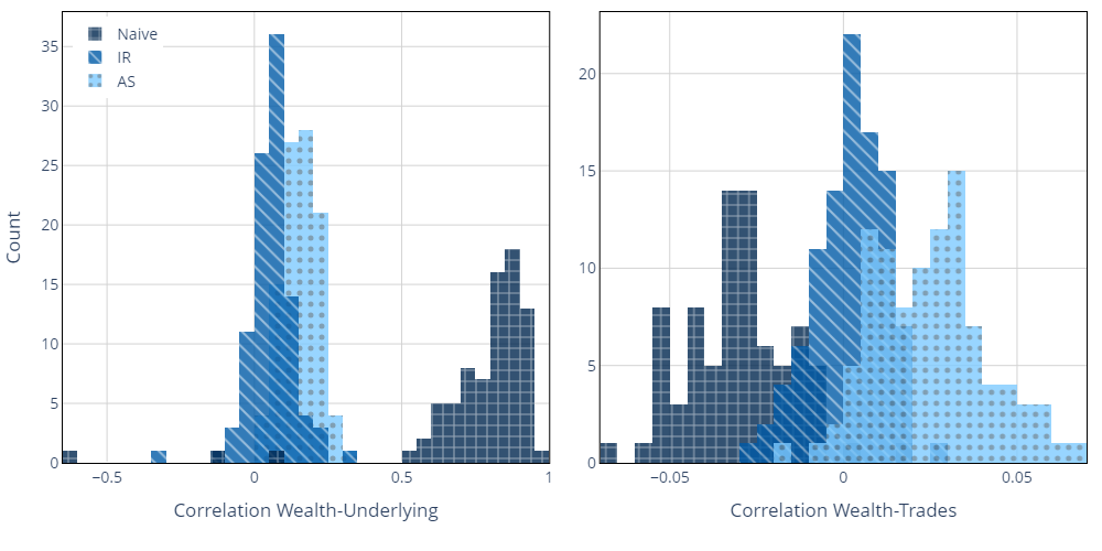
Fig. 2.: Histogram of correlations for all simulation runs.

In attempting to reconcile the results with the financial objectives defined in section 5.1, it becomes apparent that neither objective is satisfied by the naive model. While the dealer is able to generate significant profits, her returns are inferior on a risk-adjusted basis benchmarked with an AS dealer. Moreover, neutrality towards trends in the underlying is not achieved, but even worse so, the naive dealer becomes a systemic risk through accumulation of stocks. The strength of the AS model emerges very tangibly by ticking the box of a majority of the objectives. Risk-adjusted returns are high and the dealer does not influence the market with her inventory, but a positive correlation to the underlying remains and it is yet to be understood how receptive the accumulation of stock is towards parameter sensitivity. The IR model clearly lacks performance and trades off risk adjusted returns for strictly managing inventory. The performance difference to the probabilistic simulation which favoured the AR model is sizeable and demonstrates the need for a more realistic simulation environment. Thus, the next sections will delve into greater detail on the sensitivities of the dealer’s parametrisation.

5.3 Optimal Behaviour of Liquidity Providers

In this section the optimal behaviour of liquidity providers will be analysed by simulating different preference specifications. In particular, I study how risk aversion preferences, maximum order size limitations and inventory skewness (IR model only) influence optimal behaviour.

Risk aversion influences the dealer’s behaviour in two distinct ways:

1. Higher risk aversion tilts the reservation price away from the inventory side. To be precise, assuming the dealer has a long position in the stock, a higher risk aversion will lower the reservation price and vice versa. The dealer is offering to sell down her inventory at a lower price than traded in the market or is willing to collect more stocks but only at a discount. The same logic can be applied to a short position in the asset.

2. The quoted bid-ask spread around the reservation price is wider for higher risk aversion. This implies a more conservative stance of the dealer as she requires a larger premium for providing liquidity.

As can be seen in Figure 5.3, both type of dealers experience higher wealth growth at increasing levels of risk aversion. A significant gap opens in favour of the AS model which outperforms the IR model by large margins. However, while favouring higher levels of risk aversion, the AS dealer’s improvement experiences diminishing marginal returns. In contrast, the IR model has a seemingly linear effect in improvement. The reason lies in the statistical properties of the order book: Given that the quotes are set wider, the probability of being executed on the resting orders becomes increasingly low, which in turn reduces the trading frequency and so the number of opportunities one can capitalise on.

Contrasting, lowering risk aversion comes at an increasing downside. This is aggravated by the fact that quotes will be at the top-of-the-book most of the time and thus putting chances high that taking the trade with the stylised traders too early at prices too close to the mid. From a different perspective, the premium one can gain from the bid-ask spread narrows through self-inflicted behaviour of the dealer. These effects are intensified by the constant order size of the AS model, while the IR model can mitigate them via the prudent inventory management rules. This is visible in the lower threshold that both strategies show at the lower end of the parameter range where the AS dealer starts to significantly underperform its counterpart.

Considering the variance of their returns and taking a closer look into the trading volume, it becomes obvious that the AS model outperforms because it is able to trade and hold a higher amount of shares. While the average trade size is twice as large for the AS model compared to the AR model, the average inventory grows exponentially supporting this fact. On a risk-adjusted basis, the IR model can reach fairly high Sharpe ratios at the maximum parameter range which is supported by the unchanging volatility. The AS agent requires fairly low risk aversion levels to maximise risk-adjusted returns and will not see any benefits of further increases due to compensating effects of volatility which originates from longer holding periods and larger inventory of stocks. Higher order moments like skewness and kurtosis benefit from increasing risk aversion. Allowing the IR agent to adjust her risk aversion leads to a significantly better achievement of the performance objectives compared to the baseline but is still outperformed by the AS model.

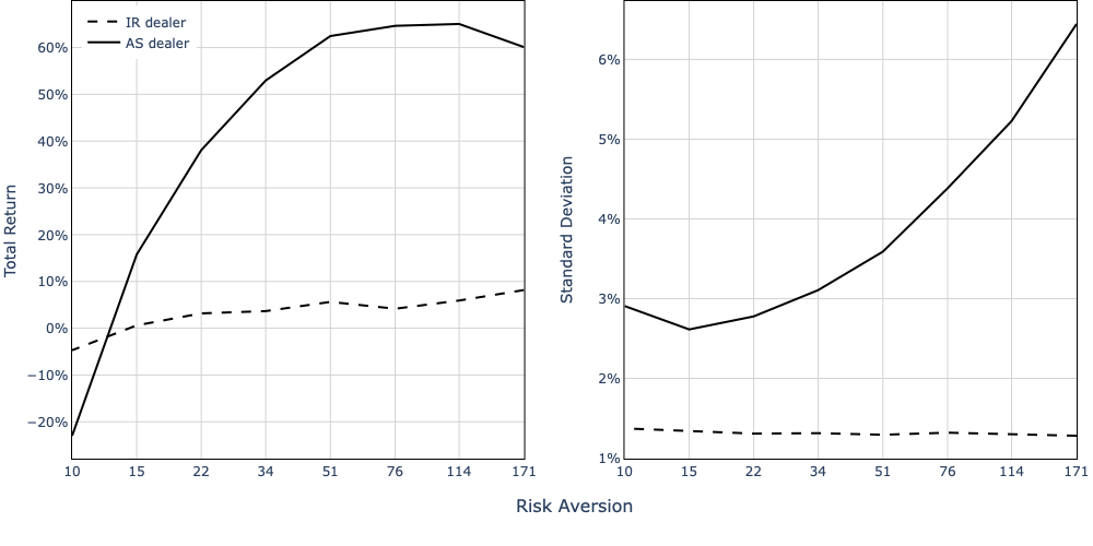
Fig. 3.: The sensitivity of wealth return statistics such as standard deviation and total return to changes in the dealer’s risk aversion. Note that the x-axis displays risk aversion as $\frac{2}{\gamma}$.

Exploring the sensitivity towards the maximum order size, asymmetric effects emerge. I observe a similar pattern in adjusting maximum order size as I did for changes in risk aversion: The AS dealer experiences diminishing returns for increasing order size. The results are visualised in Figure 5.3. Strikingly, a very asymmetric quoting, e.g. low ask (bid) quote and high bid (ask) quote leads to negative returns, also lower than the IR dealer. This is related to the fact that when building up stock position with a larger bid size, the agent cannot balance back the inventory similarly fast with a lower ask size and vice versa. It is supported by the significantly higher volatility of wealth returns at a high degree of quote asymmetry and an average inventory that is tilted to the positive side for larger bid size. Interestingly the skewness increases for the asymmetric quoting and kurtosis sinks. The latter is attributable to the increased variance of the inventory position which results in a higher wealth volatility and as such creates a wider distribution. The effects on skewness do not seem to follow a fundamental reason and as such are not possible to explain. To conclude on asymmetric quote sizes, both dealer experience a significant increase in magnitude of correlation of their wealth to the underlying towards unity, both positive and negative depending on the tilt of the quote size. This is introduced by the accumulation of inventory that is not easily balanced off any more and thus is also sub-optimal from the risk objectives perspective.

While the IR dealer sees impacts of total return on a much smaller scale, she prefers lower order sizes and does not have any asymmetric effects. Additionally, her volatility of wealth returns is much more contained but she experiences worse 3rd and 4th moments overall. Surprisingly both dealers experience shrinking correlation of wealth and underlying return with increasing (symmetric) order size in line with better risk objectives. The correlation for the AS dealer sinks from 0.25 towards 0.15 whereas the IR dealer sees a drop from 0.1 to 0.05. While not fully explainable it appears to be related to the increasing correlation of wealth and trades, which rise towards zero from low negative values.

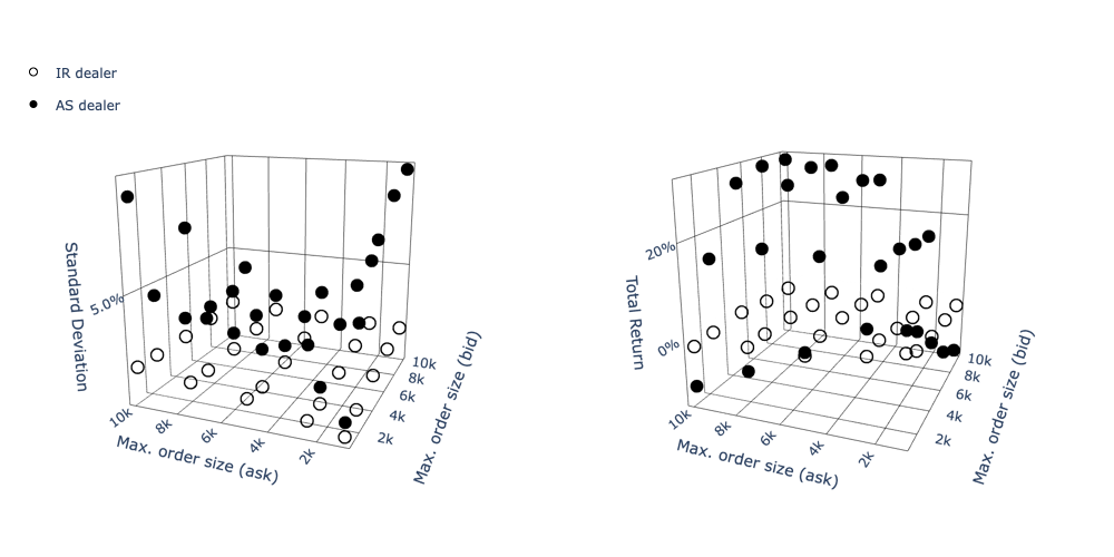
Fig. 4.: The sensitivity of wealth return statistics such as standard deviation and total return to changes in the dealer’s maximum order size $\phi^{max}$.

As inventory skew is only relevant to our IR agent, this part cannot be compared to the AS model. When lowering the inventory skew towards zero the quote size will approach the maximum ($\phi^{max}$) that is also used by the AS dealer. It is visible in Figure 5.3 that the total return increases significantly and comes close to ranks achieved by the AS dealer at lowest skew levels. This is accomplished by removing restrictions on the inventory accumulation and rather letting it be dictated by the market. That is also the reason why correlation of wealth to the underlying increases at the lowest specification simulated. Contrary to the AS model, the IR dealer does not tilt her reservation price but rather keeps it constant and thus does not alter the probability of keeping inventory as neutral as possible. This is supported by a large increase of the average inventory size and volatility, which rises to nearly three-fold of the base specification. A slightly lower skew than in the base specification however leads also to a large increase in total returns (to about 26%) without the negative side effects just mentioned and by that maximises risk-adjusted returns. The strategy is able also to perform closely to the AS model on a risk adjusted basis. Similarly to the already analysed asymmetric max. order size, asymmetric inventory skew results in accumulation of stock, along with it a high correlation to the underlying and, thus, can be rejected from the optimality discussion.

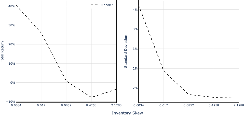
Fig. 5.: The sensitivity of wealth return statistics such as standard deviation and total return to changes in the dealer’s inventory skew $\eta$ in absolute terms. The graph shows symmetric inventory skew for bid and ask. Note that parameters are scaled by factor 100 for better readability and are displayed on a log-scale.

Both dealer strategies show great differences in their wealth moments and as such possess partly contrasting preferences towards their parameter specification. Ultimately both AS and IR dealer are able to meet financial performance as well as risk objectives and at the same time also optimise the their relevant metrics. While both dealer prefer higher risk aversion, the IR model prefers the highest specification in terms of risk-adjusted returns whereas the AS model does best for low-to-middle risk aversion levels. Both models show congruent distaste for asymmetric order size. In regard to symmetric quoting, the IR model prefers lower order size with which she comes close to the Sharpe ratios gained by the AS dealer. The AS dealer, here again, sees diminishing risk-adjusted returns and can already reap all benefits with max. order size of medium range (at around 5000 shares). The IR dealer can adjust her inventory skew towards the lower tested spectrum to increase the total return significantly. Going to the lowest inventory skew results in a similar behaviour as in the naive strategy since the reference price is not tilted to balance the inventory.

5.4 The Effects on Price Discovery

After carefully examining the optimal behaviour of the dealers, it is now time to understand their impact on market dynamics and other agents.

While being an important determinant in personal wealth for both dealers, risk aversion in the IR model has no significant effects on market dynamics. However for the AS model, higher risk aversion results in greater market volatility and a lower return kurtosis as shown in Figure 5.4. The lower return kurtosis is a direct consequence of the increased volatility which in turn stems from a larger bid-ask spread of the dealer so that the price has more room to fluctuate. If an order arrives to the market, it will be first matched at price priorities and if large enough it will be eventually matched with the dealer. However, in such a situation it is highly unlikely that it will not be filled completely and matched against the quotes further away from the mid. It can be thought as if the dealer sets a hard stop for the price to fluctuate above or below her quotes. From a different perspective, the likelihood of hitting a dealer order with lower risk aversion is increased along with the likelihood that the order ripples through the LOB and as such increases the tails. Notably, a market with an AS dealer experiences a generally lower level of kurtosis and volatility as compared to the IR dealer.

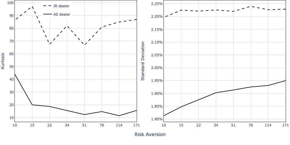
Fig. 6.: The sensitivity of market return statistics such as kurtosis and standard deviation to changes in the dealer’s risk aversion. Note that the x-axis displays risk aversion as $\frac{2}{\gamma}$.

Similarly, stylised agents are not affected by the IR strategy but show some effects in the AS model. Here, fundamentalists are the major beneficiaries and can increase their total return. This can be explained by their superior information regarding the fundamental price which they can exploit more easily given a lower bid-ask spread at low risk aversion.

For both dealers, a larger order size lowers market volatility, as shown in Figure 5.4. Contrary to the findings for risk aversion, a larger order size also lowers the market returns’ kurtosis. The principle mechanism is that a higher order size acts like a roadblock for incoming orders, as described above. The larger the size, the smaller the probability that an order can pass it. Comparably, also stylised agents benefit from a larger max. order size. Both, fundamentalist and chartist exhibit higher total returns, lower volatility and kurtosis of wealth which results in superior Sharpe ratios. The effects of larger order size are more pronounced in markets operated with an AS dealer.

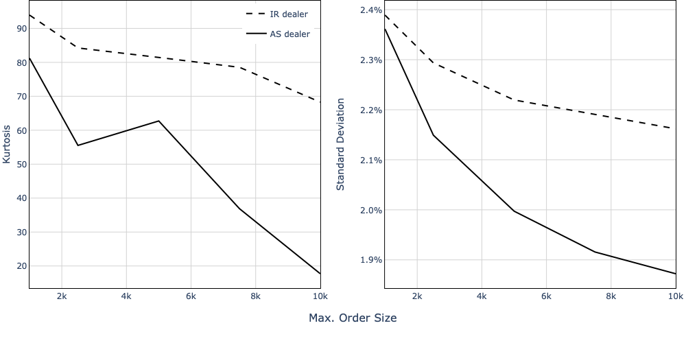
Fig. 7.: The sensitivity of market return statistics such as kurtosis and standard deviation to changes in the dealer’s max. order size.

As expected from a lower inventory skew it lowers market volatility around 20% and is established through larger dealer quotes and longer time in force. Through the lower skew, the size of the quote is less drastically reduced and, consequently, translates into limit orders being longer in the market. Note that if saturated, the IR dealer can even reduce the quote to zero, which is less likely the lower the inventory skew. The influence on market kurtosis is unintuitive at first as it peaks at the base specification and drops by 35% and 58%, both, in the directions of larger and lower inventory skew. While the drop in kurtosis towards lower skewness is related to larger absorption rate of trades of stylised agents and leads to a similar effect as increasing order size, the impact from higher skewness seems to stem from the larger variance which in turn lowers the kurtosis of market returns. Lower market volatility also translates into stylised agent wealth. While the chartists benefit from higher risk adjusted returns at lower inventory skew, which are both driven by lower volatility and higher total returns, fundamentalists’ Sharpe ratios suffer from it. They are favoured by higher skewness but experience diminishing marginal risk-adjusted returns which are already maximised by the base specification. The additional return gained through higher skew is offset by the larger volatility. However, all stylised agents experience negative wealth evolution here as well.

Putting preferences and market impact together, both mutually beneficial but also detrimental behaviour can be derived. As laid out in the previous section, the optimum from a risk-adjusted return perspective in the AS model is in the low-to-mid range of risk aversions, and, hence does not lower volatility as much as it can but reduces kurtosis. Here, the IR strategy’s impact on the market is comparably small. The question about optimality from an objective perspective cannot be answered as the preferences from other market participants are not known. In particular this relates to the trade-off whether agents prefer lower volatility or kurtosis. The AS and IR models show opposite effects on their wealth concerning the order size. While the later prefers lower order size the former favours larger size, but comes at a diminishing return. Markets clearly honour larger quote size as is apparent in both lower kurtosis and volatility. This results in market-aligned behaviour of AS dealer while the IR model’s impact is generally negative. Lower inventory skew imposes positive effects on the market by both lowering volatility and kurtosis along with being preferred by the IR dealer who can increase her performance significantly. The effects on stylised agents are ambiguous as chartists clearly benefit from lower inventory skew while fundamentalists suffer and vice versa. For the IR model, the total effect is somewhat compensating as the dealer would favour lower order size and lower skewness. As just mentioned, the latter would be beneficial for market dynamics while the first would be partially counteracted.

6 Conclusion

This paper developed an agent-based model which centres around a limit orderbook allowing market participants to share information and thereby lead price discovery. Market participants are three types of stylised agents - fundamentalists, chartists and noise traders - additionally I introduce passive dealers who act as liquidity providers. The importance of agent-based modelling for trading simulation is shown by providing evidence of different conclusions depending on which framework to use as a test bed. The probabilistic model neglects dynamic interactions and endogenous behaviour that are an important part of real financial markets. As such, evidence was presented that naive dealer strategies accumulate large amount inventory and experience large correlations of their wealth to the underlying, which both could be found through the agent-based framework. The extension by Fushimi and González Rojas (2018) (IR dealer) showed much lower performance when deploying it in an agent-based simulation and was outperformed by the model developed in Avellaneda and Stoikov (2008) (AS dealer).

Both dealer models have been further studied to understand their preferences and subsequent effects on market dynamics. Dealers have commonalities by preferring higher risk aversion as it significantly impacts their wealth. However, this has ambiguous effects on the market which is visible in higher return volatility but shallower tails. With respect to max. order size, the AS model benefits from larger quotes which was shown to be in the interest of markets by reducing both volatility and kurtosis. By comparison, the IR dealer prefers lower quote size and would in fact impact markets negatively. Inventory skewness has large implications for the dealer’s wealth as she prefers to lower her quote size moderately and, thus, also has positive impact market dynamics. At the same time chartist benefit but fundamentalists are disadvantaged, both of which is visible in their total returns. The analysis has shown that agent’s returns clearly depends on the dealer’s implementation what her preferences are and how those loop back to market dynamics.

This work uncovered some important relationships between preference parameters on market dynamics and wealth evolution. This framework can be extended to include other variables by incorporating completely new rules or environments similar to the work done by Vuorenmaa and Wang (2014). However, the model should remain tractable when introducing significant extensions. Future work can include more realistic behaviour of stylised agents to make them profitable or a more active market maker strategy.

A

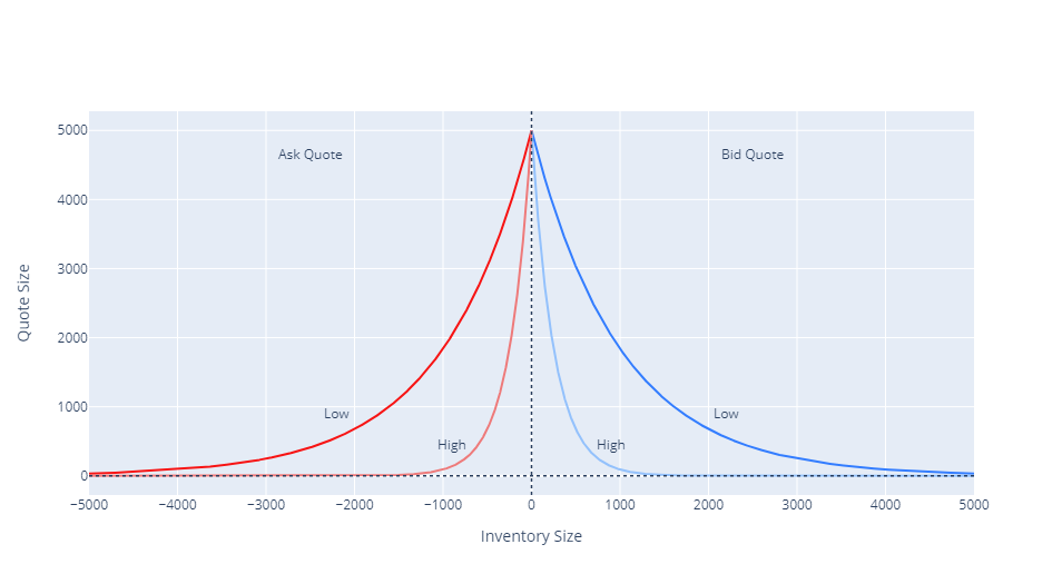
Fig. 8.: Demonstration of effects of low and high inventory skew on quote size given different values of inventory size. High (low) inventory skew leads to faster (slower) decay of quoted volume in the direction inventory. Maximum order size is set at 5000, low (high) skew demonstrates a parameter value of 0.001 (0.004).

References

- Andrei A. Kirilenko et al. (2011) Andrei A. Kirilenko, Albert S. Kyle, Mehrdad Samadi, Tugkan Tuzun, 2011. The flash crash: The impact of high frequency trading on an electronic market. SSRN Electronic Journal .