SGNet: Structure Guided Network via Gradient-Frequency Awareness
for Depth Map Super-Resolution
Abstract
Depth super-resolution (DSR) aims to restore high-resolution (HR) depth from low-resolution (LR) one, where RGB image is often used to promote this task. Recent image guided DSR approaches mainly focus on spatial domain to rebuild depth structure. However, since the structure of LR depth is usually blurry, only considering spatial domain is not very sufficient to acquire satisfactory results. In this paper, we propose structure guided network (SGNet), a method that pays more attention to gradient and frequency domains, both of which have the inherent ability to capture high-frequency structure. Specifically, we first introduce the gradient calibration module (GCM), which employs the accurate gradient prior of RGB to sharpen the LR depth structure. Then we present the Frequency Awareness Module (FAM) that recursively conducts multiple spectrum differencing blocks (SDB), each of which propagates the precise high-frequency components of RGB into the LR depth. Extensive experimental results on both real and synthetic datasets demonstrate the superiority of our SGNet, reaching the state-of-the-art (see Fig. 1). Codes and pre-trained models are available at https://github.com/yanzq95/SGNet.
Introduction
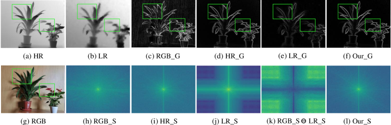
Image guided DSR has been widely applied in various fields, such as 3D reconstruction (Yuan et al. 2023a), virtual reality (Bonetti, Warnaby, and Quinn 2018), and augmented reality (Xiong et al. 2021). However, the blurry structure of LR depth caused by complex imaging environment still impedes their performance. For example, Fig. 2 (LR) shows that, the LR depth contain rich low-frequency content but are severely deficient in clear high-frequency structure. Recently, many DSR approaches (Yuan et al. 2023a; Shi, Ye, and Du 2022) are proposed to tackle this issue. However, most of them focus only on the spatial domain for recovery, which is not very sufficient to obtain desired results.
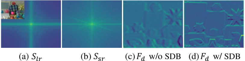
For one thing, from (c)-(f) of Fig. 2 we discover that, the gradient features of RGB and HR contain highly discriminative object structure. Besides, although the degraded LR is terribly blurry, the gradient feature can still delineate its structure clearly. For another thing, from (h)-(j) of Fig. 2 we find that, the spectrum features of RGB and HR reserve not only low-frequency content (central area) but also high-frequency structure (corner area). In contrast, the spectrum feature of LR lacks a large number of high-frequency components. These evidences indicate that the gradient and spectrum information can accurately depict the distribution of high-frequency structure. Consequently, motivated by these two observations, in this paper we pay more attention to gradient and frequency domains to take advantage of their inherent properties for clear structure recovery.
Gradient domain. We design the gradient calibration module (GCM) to leverage the powerful structure representation capability of gradient feature. Specifically, RGB and LR are first mapped into gradient domain (Ma et al. 2020). Then the accurate RGB gradient prior is employed to calibrate the blurry structure of LR. Besides, we introduce a gradient-aware loss to further sharpen the structure via narrowing the distance between the intermediate feature of GCM and that of HR in gradient domain.
Frequency domain. We present the Frequency Awareness Module (FAM), which recursively conducts multiple spectrum differencing blocks (SDB) to propagate the precise high-frequency components (Yan et al. 2022b) of RGB. Concretely, SDB first maps RGB and LR into the same frequency domain. To explicitly compensate for the absent high-frequency components, i.e., the blank corner area of Fig. 2(j), SDB next employs subtraction between the spectrum feature of RGB and that of LR in Fig. 2(k), which is then merged with the spectrum feature of LR to enhance the structure. Besides, we initiate a frequency-aware loss to further strengthen the response of FAM in frequency space.
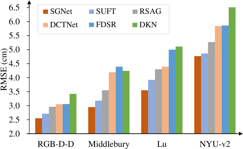
Owing to the ingenious designs of GCM and FAM, (f) and (l) of Fig. 2 show that our approach can obtain very sharp and highlighted structure in gradient and frequency domains, respectively. As a result in Fig. 1, our SGNet surpasses the five state-of-the-art methods by 16% (RGB-D-D), 24% (Middlebury), 21% (Lu) and 15% (NYU-v2) in average. In summary, our contributions are as follows:
-
•
Apart from the spatial domain, we introduce a novel perspective that exploits the gradient and frequency domains for the structure enhancement of DSR task.
-
•
We propose SGNet that consists of novel GCM and FAM, where GCM leverages the gradient prior to adaptively calibrate and sharpen LR structure, whilst FAM employs recursive SDB to propagate the high-frequency components into LR for clear structure recovery.
-
•
SGNet achieves significantly superior performance on both real-world and synthetic datasets. Codes and pre-trained models are released for peer research.
Related Work
Depth Map Super-Resolution
Benefiting from the rich structure of RGB image, guided DSR (Song et al. 2020; Yang et al. 2022; Zhong et al. 2021) have attracted broad attention. For example, (Shi, Ye, and Du 2022) introduce a symmetric uncertainty method to select RGB information that is effective for HR depth recovery whilst skipping harmful texture. (Kim, Ponce, and Ham 2021) design joint image filtering to adaptively output the neighbors and their weights for each pixel. (Deng and Dragotti 2020) propose a multi-modal convolutional sparse coding to automatically split common and private features among different modalities. Similarly, (Zhao et al. 2022) build a discrete cosine network that extracts both shared and specific multi-modal information through a semi-decoupled feature extraction module. Besides, some methods present multi-task learning frameworks to leverage complementary knowledge. For instance, (Yan et al. 2022a) introduce an auxiliary depth completion branch to propagate the correlation of dense depth into the DSR branch. (Tang et al. 2021) transmit RGB into a space that is close the depth space via depth estimation, thus facilitating the RGB-D fusion for DSR. Furthermore, (Sun et al. 2021) develop cross-task knowledge distillation to exchange correlation between DSR and depth estimation branches. Most recently, (Yuan et al. 2023a) propose recursive structure attention to gradually estimate high-frequency structure. Meanwhile, (Yuan et al. 2023b) design a structure flow-guided network to learn the edge-focused guidance feature for depth structure enhancement. In addition, graph regularization (De Lutio et al. 2022) and anisotropic diffusion (Metzger, Daudt, and Schindler 2023) are applied to enhance the recovery of depth structure. Different from these approaches, most of which concentrate only on spatial domain, we pay more attention to gradient and frequency domains, employing the high-frequency components of RGB to guide depth structure.
Gradient and Frequency Learning
Since the inherent characteristics of gradient and spectrum are quite helpful to represent structure, various related methods (Sun, Xu, and Shum 2010; Lin et al. 2023) have been proposed. In gradient domain, (Qiao et al. 2023) employ low-cut filtering to extract gradient information and then fuse at multiple scales and stages for DSR. (Sun, Xu, and Shum 2010) introduce a gradient field transformation to constrain the gradient fields of the HR image during the execution of SISR. (Ma et al. 2020) develop a structure-preserving method for single image super-resolution (SISR), which propagates gradient knowledge into the RGB branch. (Zhu et al. 2015) build a gradient pattern dictionary to simulate deformable gradient of SISR. In frequency domain, (Zhou et al. 2022b, c) integrate spatial and spectrum features for multi-spectrum pan-sharpening. (Jiang et al. 2021) design a focal frequency loss to narrow the frequency domain gap between real image and generated image. (Mao et al. 2023) introduce a frequency selective network to adaptively learn kernel-level features for image deblurring. (Lin et al. 2023) carry out frequency-enhanced variational autoencoders to restore the high-frequency components lost during the image compression process. Inspired by these methods, we employ the gradient and spectrum of RGB to fully guide depth structure in both gradient and frequency domains.
Method
Problem Formulation
Given input LR depth and HR RGB image , guided DSR aims to predict HR depth that is supervised by HR ground-truth depth . , , refer to the height, width, and scaling factor, respectively.
Network Architecture
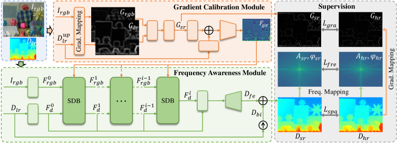
As illustrated in Fig. 3, the proposed SGNet is mainly composed of two modules, i.e., Gradient Calibration Module (GCM) and Frequency Awareness Module (FAM) that contains multiple Spectrum Differencing Blocks (SDB), aiming to recover more accurate depth structure in gradient and frequency domains, respectively.
Firstly, RGB and up-sampled depth are fed into GCM, obtaining gradient representation and by gradient mapping (Ma et al. 2020). Secondly, some residual groups (Zhang et al. 2018) and channel attention (Woo et al. 2018) are involved to calibrate the gradient of via , yielding that is with the same resolution as . Thirdly, GCM outputs the guided feature by down-sampling the sum of the gradient feature and spatial feature . Fourthly, and are encoded to generate and respectively, both of which are then input into the first SDB of FAM together with . Fifthly, FAM recursively conducts SDB to obtain . Finally, the HR prediction is produced by summing and the bicubic interpolation of . During training process, our SGNet employs three loss functions of different domains, i.e., gradient-aware loss , frequency-aware loss and spatial-aware loss . Specifically, takes as input and the gradient mapping of ground-truth , while inputs the corresponding mappings of and .
Gradient Calibration Module
Our GCM is depicted in the orange part of Fig. 3. We first employ a gradient mapping function (Ma et al. 2020) to transmit and into gradient domain. Specifically, given input , the general definition of is:
| (1) |
where refers to the pixel value at coordinates . Then the gradient features of and are mapped as:
| (2) |
Next we conduct that is composed of two residual groups (Zhang et al. 2018) and a channel attention block (Woo et al. 2018), to calibrate the gradient of , obtaining :
| (3) |
Supposing that the residual groups (orange and green rectangles in Fig. 3) are denoted as . Then, we fuse the gradient feature and depth feature to sharpen the depth structure. Finally, a down-sampling convolution is deployed to decrease the resolution from to , yielding the gradient-enhanced depth feature :
| (4) |
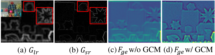
Fig. 4 (b) and (d) show that our GCM successfully produce very clear gradient feature and sharp depth feature.
Frequency Awareness Module
Our FAM is shown in the green part of Fig. 3. The input and are first mapped as:
| (5) |
Next, given the gradient-enhanced feature , and , FAM recursively conducts SDB to refine depth feature:
| (6) |
where refers to ith SDB. To leverage all of the history depth features, FAM concatenates . Then FAM encodes the combined feature via a residual group and an up-sampling convolutional layer to produce the frequency-enhanced feature . Finally, FAM outputs the predicted HR depth by fusing with , i.e., the bicubic interpolation result of :
| (7) |
where denotes concatenation.
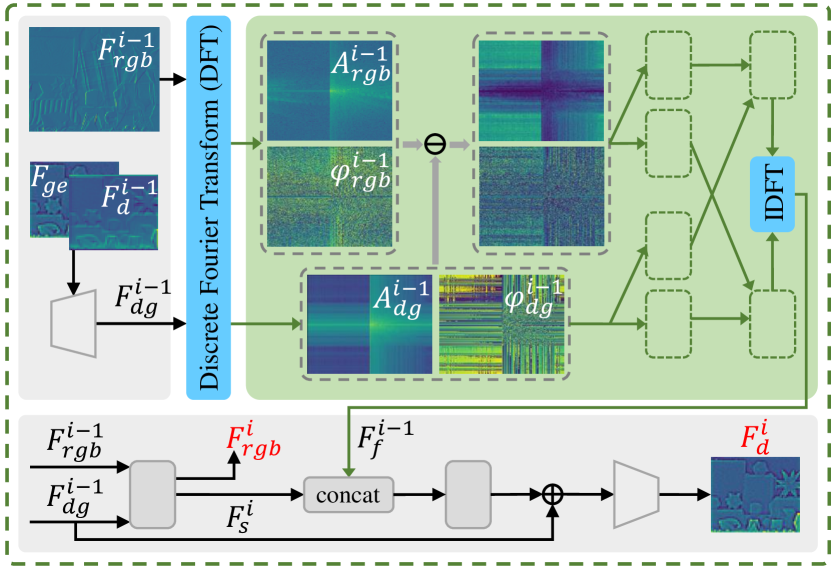
Spectrum Differencing Block.
Fig. 5 shows that SDB first fuses and up-samples and with a convolution and , producing HR :
| (8) |
Next, the discrete fourier transform (DFT) is employed to map and into the frequency domain, generating RGB spectrum and depth spectrum , both of which are decomposed into amplitude and phase:
| (9) |
where and . denotes spectral decomposition function. and refer to the amplitude and phase of , respectively, while and are the amplitude and phase of .
AS depicted in the green part of Fig. 5, we first calculate the amplitude subtraction and phase subtraction between and to produce and , both of which are fed into multiple convolutional layers followed by activation function to learn high-frequency knowledge. Meanwhile, we also perform to extract the spectrum features of and . Then, the inverse discrete fourier transform (IDFT) is employed to map the fused amplitude feature and phase feature into spatial domain, producing :
| (10) |
where consists of a convolution and concatenation.
Finally, to strengthen the correlation between spatial domain and frequency domain, we employ the invertible neural network (Zhou et al. 2022a) and down-sampling to fuse the spatial domain feature and :
| (11) |
where . and refer to the output depth feature and RGB feature of ith SDB, respectively. As shown in Fig. 6 (b) and (d), our SDB succeeds recovering high-frequency components and clear structure.
| Scale | Bicubic | TGV | DJF | DMSG | GbFT | DKN | FDSR | CTKT | DCTNet | AHMF | RSAG | SUFT | SGNet |
|---|---|---|---|---|---|---|---|---|---|---|---|---|---|
| 8.16 | 4.98 | 3.54 | 3.02 | 3.35 | 1.62 | 1.61 | 1.49 | 1.59 | 1.40 | 1.23 | 1.12 | 1.10 | |
| 14.22 | 11.23 | 6.20 | 2.99 | 5.73 | 3.26 | 3.18 | 2.73 | 3.16 | 2.89 | 2.51 | 2.51 | 2.44 | |
| 22.32 | 28.13 | 10.21 | 9.17 | 9.01 | 6.51 | 5.86 | 5.11 | 5.84 | 5.64 | 5.27 | 4.86 | 4.77 |
| Scale | Bicubic | SDF | DJF | PAC | DJFR | DKN | FDKN | FDSR | JIIF | DCTNet | RSAG | SUFT | SGNet |
|---|---|---|---|---|---|---|---|---|---|---|---|---|---|
| 2.00 | 4.06 | 3.41 | 1.25 | 3.35 | 1.30 | 1.18 | 1.16 | 1.17 | 1.08 | 1.14 | 1.10 | 1.10 | |
| 3.23 | 5.51 | 5.57 | 1.98 | 5.57 | 1.96 | 1.91 | 1.82 | 1.79 | 1.74 | 1.75 | 1.69 | 1.64 | |
| 5.16 | 7.39 | 8.15 | 3.49 | 7.99 | 3.42 | 3.41 | 3.06 | 2.87 | 3.05 | 2.96 | 2.71 | 2.55 |
| Methods | Middlebury | Lu | ||||
|---|---|---|---|---|---|---|
| DJF | 1.68 | 3.24 | 5.62 | 1.65 | 3.96 | 6.75 |
| DJFR | 1.32 | 3.19 | 5.57 | 1.15 | 3.57 | 6.77 |
| FDKN | 1.08 | 2.17 | 4.50 | 0.82 | 2.10 | 5.05 |
| DKN | 1.23 | 2.12 | 4.24 | 0.96 | 2.16 | 5.11 |
| FDSR | 1.13 | 2.08 | 4.39 | 1.29 | 2.19 | 5.00 |
| DCTNet | 1.10 | 2.05 | 4.19 | 0.88 | 1.85 | 4.39 |
| RSAG | 1.13 | 1.74 | 3.55 | 0.79 | 1.67 | 4.30 |
| SUFT | 1.07 | 1.75 | 3.18 | 1.10 | 1.74 | 3.92 |
| SGNet | 1.15 | 1.64 | 2.95 | 1.03 | 1.61 | 3.55 |
Loss Function
Given RGB-D pairs, a spatial-aware loss is used:
| (12) |
Next we utilize a gradient-aware loss to facilitate the calibration of LR gradient information:
| (13) |
where denote the ground-truth gradient.
Then we introduce a frequency-aware loss to learn the HR spectrum, which consists of an amplitude loss and a phase loss :
| (14) |
where and severally refer to the amplitude and phase of the HR depth prediction, while and correspond to those of the ground-truth depth. and are hyper-parameters.
Finally, the total training loss is defined as:
| (15) |
where , are hyper-parameters.
Experiments
Experimental Settings
Datasets.
We conduct experiments on both synthetic NYU-v2 (Silberman et al. 2012), Middlebury (Hirschmuller and Scharstein 2007; Scharstein and Pal 2007), Lu (Lu, Ren, and Liu 2014), and real-world RGB-D-D (He et al. 2021) datasets. Following previous works (Sun et al. 2021; Yuan et al. 2023a; Zhao et al. 2023), on NYU-v2 dataset, the training set contains 1000 RGB-D pairs, while the test set consists of 449 pairs. Besides, the pre-trained model on NYU-v2 is also tested on Middlebury (30 pairs), Lu (6 pairs), and RGB-D-D (405 pairs). In these synthetic scenarios, the LR depth input is produced by bicubic down-sampling from the HR depth ground-truth. To validate the generalization of our method in real-world environment, we implement our SGNet on the real-world RGB-D-D dataset, including 2,215 RGB-D pairs for training and 405 for testing, where the LR depth is obtained via the ToF camera of Huawei P30 Pro.
Metrics and Implementation Details.
Following previous methods (Kim, Ponce, and Ham 2021; Zhao et al. 2022), the root mean square error (RMSE) in centimeter is employed as the evaluation metric. During the training, we randomly crop the RGB image and HR depth into . Adam optimizer (Kingma and Ba 2014) with an initial learning rate of is used to train SGNet with a single TITAN RTX GPU. The hyper-parameters are set as , and .
Comparison with the state-of-the-art
Tabs. 1-4 compare SGNet with state-of-the-art methods on , and DSR, including TGV (Ferstl et al. 2013), SDF (Ham, Cho, and Ponce 2017), DJF (Li et al. 2016), DJFR (Li et al. 2019), PAC (Su et al. 2019), DMSG (Hui, Loy, and Tang 2016), GbFT (AlBahar and Huang 2019), DKN (Kim, Ponce, and Ham 2021), FDKN (Kim, Ponce, and Ham 2021), FDSR (He et al. 2021), JIIF (Tang, Chen, and Zeng 2021), CTKT (Sun et al. 2021), AHMF (Zhong et al. 2021), DCTNet (Zhao et al. 2022), SUFT (Shi, Ye, and Du 2022) and RSAG (Yuan et al. 2023a).
Quantitative Comparison.
Overall, Tabs. 1-4 report that our SGNet achieves state-of-the-art performance on both the synthetic (Tabs. 1-3) and real-world (Tab. 4) datasets. Specifically, From Tabs. 1 and 2 we observe that SGNet is superior to the most of other methods on NYU-v2 and RGB-D-D datasets. For example, compared to the second best methods, our SGNet decreases the RMSE by (NYU-v2) and (RGB-D-D) on DSR. Besides, Tab. 3 verifies the generalization ability of our SGNet on Middlebury and Lu datasets. We discover that our SGNet is significantly superior to others on and DSR and obtains competitive result on DSR. When comparing to the suboptimal methods on DSR, the RMSE of our SGNet is (Middlebury) and (Lu) lower.
Tab. 4 lists the comparison on the real-world RGB-D-D dataset. Following previous methods (Zhao et al. 2022; Yuan et al. 2023a), we first test the pre-trained models of NYU-v2 on RGB-D-D (without *), then retrain and test FDSR, DCTNet, SUFT and SGNet on RGB-D-D (with *). We find that both our SGNet and SGNet* achieve the best performance. For example, SGNet* surpasses the second best SUFT* by in RMSE. In short, these evidences confirm that SGNet contributes to better performance and generalization.
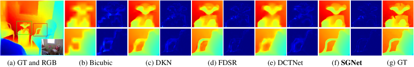
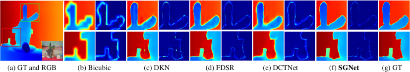
Visual Comparison.
Figs. 7-9 present visual comparison results. Obviously, our method can restore more precise depth predictions with clearer and sharper structure. For example, the edges of chair and doll in () in Figs. 7 and 8 are more discriminative than others, while the errors maps shows the higher accuracy. Although previous methods that mainly focus on spatial domain are able to recover the most of depth information, the detailed structure is still difficult to predict. In contrast, our SGNet pays more attention to both gradient and frequency domains to leverage their inherent advantages of modeling structure.
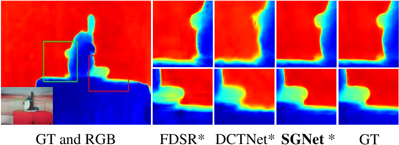
Furthermore, the DSR task is more challenging in real-world scenarios because the LR depth is often blurry and distorted. Fig. 9 demonstrates the visual comparison on the real-world RGB-D-D dataset. Compared to the state-of-the-art FDSR* and DCTNet*, our SGNet* can obtain more accurate HR depth with clear structure that is very close to the ground-truth depth. These visual results validate that our method can effectively enhance depth structure.
| Methods | Train | RMSE | Methods | Train | RMSE |
|---|---|---|---|---|---|
| DJF | NYU-v2 | 7.90 | DCTNet | NYU-v2 | 7.37 |
| DJFR | NYU-v2 | 8.01 | SUFT | NYU-v2 | 7.22 |
| FDKN | NYU-v2 | 7.50 | FDSR* | RGB-D-D | 5.49 |
| DKN | NYU-v2 | 7.38 | DCTNet* | RGB-D-D | 5.43 |
| FDSR | NYU-v2 | 7.50 | SUFT* | RGB-D-D | 5.41 |
| SGNet | NYU-v2 | 7.22 | SGNet* | RGB-D-D | 5.32 |
Ablation Study
GCM and FAM.
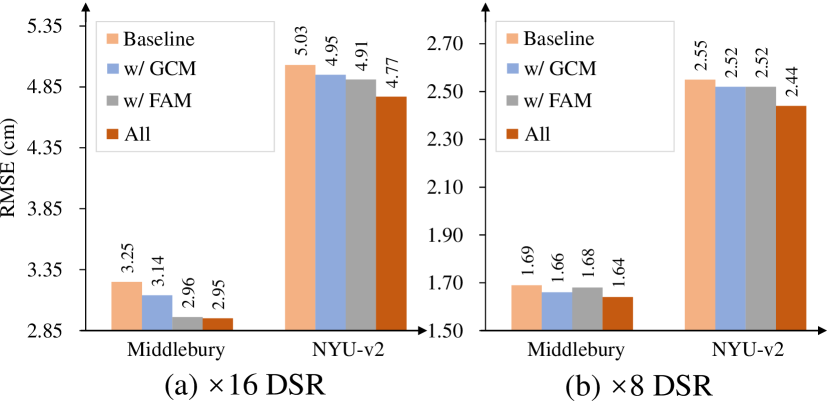
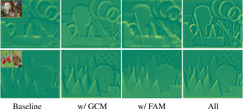
Figs. 10 and 11 show the ablation study of GCM and FAM. For the baseline, we first remove GCM completely. Then in SDB (Fig. 5) of FAM, the frequency operation is removed, only retaining the bottom gray part.
As shown in Fig. 10, both GCM and FAM can reduce RMSE by propagating the high-frequency components of RGB into depth in the gradient and frequency domains. When combining GCM and FAM, SGNet achieves the best performance. For example, compared to the baseline, GCM is superior on Middlebury and on NYU-v2. FAM also reduces the error by and , respectively. Finally, our SGNet surpasses the baseline by on Middlebury and on NYU-v2.
Tab. 5 lists the complexity comparison. It is observed that GCM & FAM are lightweight, i.e., 1.68M & 0.39M cost in Parameters, 1.30G & 1.53G cost in Memory, and 235.0G & 42.6G cost in FLOPs, respectively. When GCM & FAM are combined to, the performance is significantly improved with acceptable sacrifice in complexity.
In addition, Fig. 11 illustrates the visual results of intermediate depth features. We discover that both GCM and FAM are able to generate clearer depth structure than the baseline. Furthermore, when GCM and FAM are deployed together, our SGNet can produce much sharper structure.
These numerical and visual evidences indicate that, by exploiting the structure representation in gradient and frequency domains, our SGNet can significantly enhance depth structure and thus improve the performance.
| Methods | Params (M) | FLOPs (G) | Memory (G) | Time (ms) |
|---|---|---|---|---|
| Baseline | 37.18 | 4346.3 | 8.02 | 63 |
| +GCM | 38.86 | 4581.3 | 9.32 | 69 |
| +FAM | 37.57 | 4388.9 | 9.55 | 67 |
| All | 39.25 | 4623.9 | 10.77 | 73 |
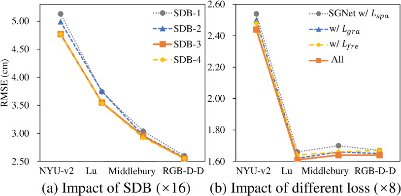
Different Recursion Numbers of SDB.
Fig. 12 (a) shows the ablation study of different numbers of SDB. The baseline is SGNet with GCM, FAM and all loss functions. It can be observed that the performance gradually improves as the number of SDB increases. When employing SDB-4, the errors decrease a little on Lu and Middlebury but maintain unchanged on NYU-v2 and RGB-D-D. Therefore, for better trade-off between the model complexity and accuracy, we select SDB-3 ( the orange solid line) as the default setting.
Different Loss Functions.
Fig. 12 (b) shows the ablation study of different loss functions. The baseline is SGNet with GCM, FAM and only. We find that both the gradient-aware and frequency-aware contribute to performance improvement. When and are deployed together, the model achieves the best performance, i.e., averagely surpassing the basic SGNet by on NYU-v2, Lu, Middlebury and RGB-D-D datasets.
Conclusion
In this paper, we proposed SGNet, a novel DSR solution that payed more attention to gradient and frequency domains, employing the high-frequency components of RGB to enhance depth structure. For gradient domain, we designed the gradient calibration module to adaptively sharpen the blurry structure of LR depth via clear RGB gradient prior. For frequency domain, we developed the frequency awareness module, which recursively conducted multiple spectrum differencing blocks to propagate the high-frequency knowledge of RGB spectrum into the depth. Besides, we introduced the gradient-aware loss and frequency-aware loss to further narrow the structure distance of the prediction and target in both gradient and frequency domains. Extensive experiments demonstrated that our SGNet achieved state-of-the-art performance on four benchmark datasets.
Acknowledgements
The authors thank all reviewers for their instructive comments. This work was supported by the Postgraduate Research & Practice Innovation Program of Jiangsu Province (KYCX23_0471). Note that the PCA Lab is associated with, Key Lab of Intelligent Perception and Systems for High-Dimensional Information of Ministry of Education, and Jiangsu Key Lab of Image and Video Understanding for Social Security, School of Computer Science and Engineering, Nanjing University of Science and Technology.
References
- AlBahar and Huang (2019) AlBahar, B.; and Huang, J.-B. 2019. Guided image-to-image translation with bi-directional feature transformation. In ICCV, 9016–9025.
- Bonetti, Warnaby, and Quinn (2018) Bonetti, F.; Warnaby, G.; and Quinn, L. 2018. Augmented reality and virtual reality in physical and online retailing: A review, synthesis and research agenda. Augmented reality and virtual reality: Empowering human, place and business, 119–132.
- De Lutio et al. (2022) De Lutio, R.; Becker, A.; D’Aronco, S.; Russo, S.; Wegner, J. D.; and Schindler, K. 2022. Learning graph regularisation for guided super-resolution. In CVPR, 1979–1988.
- Deng and Dragotti (2020) Deng, X.; and Dragotti, P. L. 2020. Deep convolutional neural network for multi-modal image restoration and fusion. IEEE transactions on pattern analysis and machine intelligence, 43(10): 3333–3348.
- Ferstl et al. (2013) Ferstl, D.; Reinbacher, C.; Ranftl, R.; Rüther, M.; and Bischof, H. 2013. Image guided depth upsampling using anisotropic total generalized variation. In ICCV, 993–1000.
- Ham, Cho, and Ponce (2017) Ham, B.; Cho, M.; and Ponce, J. 2017. Robust guided image filtering using nonconvex potentials. IEEE transactions on pattern analysis and machine intelligence, 40(1): 192–207.
- He et al. (2021) He, L.; Zhu, H.; Li, F.; Bai, H.; Cong, R.; Zhang, C.; Lin, C.; Liu, M.; and Zhao, Y. 2021. Towards Fast and Accurate Real-World Depth Super-Resolution: Benchmark Dataset and Baseline. In CVPR, 9229–9238.
- Hirschmuller and Scharstein (2007) Hirschmuller, H.; and Scharstein, D. 2007. Evaluation of cost functions for stereo matching. In CVPR, 1–8.
- Hui, Loy, and Tang (2016) Hui, T.-W.; Loy, C. C.; and Tang, X. 2016. Depth map super-resolution by deep multi-scale guidance. In ECCV, 353–369.
- Jiang et al. (2021) Jiang, L.; Dai, B.; Wu, W.; and Loy, C. C. 2021. Focal frequency loss for image reconstruction and synthesis. In ICCV, 13919–13929.
- Kim, Ponce, and Ham (2021) Kim, B.; Ponce, J.; and Ham, B. 2021. Deformable kernel networks for joint image filtering. International Journal of Computer Vision, 129(2): 579–600.
- Kingma and Ba (2014) Kingma, D. P.; and Ba, J. 2014. Adam: A Method for Stochastic Optimization. Computer Science.
- Li et al. (2016) Li, Y.; Huang, J.-B.; Ahuja, N.; and Yang, M.-H. 2016. Deep joint image filtering. In ECCV, 154–169.
- Li et al. (2019) Li, Y.; Huang, J.-B.; Ahuja, N.; and Yang, M.-H. 2019. Joint image filtering with deep convolutional networks. IEEE transactions on pattern analysis and machine intelligence, 41(8): 1909–1923.
- Lin et al. (2023) Lin, X.; Li, Y.; Hsiao, J.; Ho, C.; and Kong, Y. 2023. Catch Missing Details: Image Reconstruction with Frequency Augmented Variational Autoencoder. In CVPR, 1736–1745.
- Lu, Ren, and Liu (2014) Lu, S.; Ren, X.; and Liu, F. 2014. Depth enhancement via low-rank matrix completion. In CVPR, 3390–3397.
- Ma et al. (2020) Ma, C.; Rao, Y.; Cheng, Y.; Chen, C.; Lu, J.; and Zhou, J. 2020. Structure-preserving super resolution with gradient guidance. In CVPR, 7769–7778.
- Mao et al. (2023) Mao, X.; Liu, Y.; Liu, F.; Li, Q.; Shen, W.; and Wang, Y. 2023. Intriguing findings of frequency selection for image deblurring. In AAAI, 1905–1913.
- Metzger, Daudt, and Schindler (2023) Metzger, N.; Daudt, R. C.; and Schindler, K. 2023. Guided Depth Super-Resolution by Deep Anisotropic Diffusion. In CVPR, 18237–18246.
- Qiao et al. (2023) Qiao, X.; Ge, C.; Zhang, Y.; Zhou, Y.; Tosi, F.; Poggi, M.; and Mattoccia, S. 2023. Depth Super-Resolution from Explicit and Implicit High-Frequency Features. arXiv preprint arXiv:2303.09307.
- Scharstein and Pal (2007) Scharstein, D.; and Pal, C. 2007. Learning conditional random fields for stereo. In CVPR, 1–8.
- Shi, Ye, and Du (2022) Shi, W.; Ye, M.; and Du, B. 2022. Symmetric Uncertainty-Aware Feature Transmission for Depth Super-Resolution. In ACM MM, 3867–3876.
- Silberman et al. (2012) Silberman, N.; Hoiem, D.; Kohli, P.; and Fergus, R. 2012. Indoor segmentation and support inference from rgbd images. In ECCV, 746–760.
- Song et al. (2020) Song, X.; Dai, Y.; Zhou, D.; Liu, L.; Li, W.; Li, H.; and Yang, R. 2020. Channel attention based iterative residual learning for depth map super-resolution. In CVPR, 5631–5640.
- Su et al. (2019) Su, H.; Jampani, V.; Sun, D.; Gallo, O.; Learned-Miller, E.; and Kautz, J. 2019. Pixel-adaptive convolutional neural networks. In CVPR, 11166–11175.
- Sun et al. (2021) Sun, B.; Ye, X.; Li, B.; Li, H.; Wang, Z.; and Xu, R. 2021. Learning scene structure guidance via cross-task knowledge transfer for single depth super-resolution. In CVPR, 7792–7801.
- Sun, Xu, and Shum (2010) Sun, J.; Xu, Z.; and Shum, H.-Y. 2010. Gradient profile prior and its applications in image super-resolution and enhancement. IEEE Transactions on Image Processing, 20(6): 1529–1542.
- Tang, Chen, and Zeng (2021) Tang, J.; Chen, X.; and Zeng, G. 2021. Joint implicit image function for guided depth super-resolution. In ACM MM, 4390–4399.
- Tang et al. (2021) Tang, Q.; Cong, R.; Sheng, R.; He, L.; Zhang, D.; Zhao, Y.; and Kwong, S. 2021. Bridgenet: A joint learning network of depth map super-resolution and monocular depth estimation. In ACM MM, 2148–2157.
- Woo et al. (2018) Woo, S.; Park, J.; Lee, J.-Y.; and Kweon, I. S. 2018. Cbam: Convolutional block attention module. In ECCV, 3–19.
- Xiong et al. (2021) Xiong, J.; Hsiang, E.-L.; He, Z.; Zhan, T.; and Wu, S.-T. 2021. Augmented reality and virtual reality displays: emerging technologies and future perspectives. Light: Science & Applications, 10(1): 216.
- Yan et al. (2022a) Yan, Z.; Wang, K.; Li, X.; Zhang, Z.; Li, G.; Li, J.; and Yang, J. 2022a. Learning complementary correlations for depth super-resolution with incomplete data in real world. IEEE transactions on neural networks and learning systems.
- Yan et al. (2022b) Yan, Z.; Wang, K.; Li, X.; Zhang, Z.; Li, J.; and Yang, J. 2022b. RigNet: Repetitive image guided network for depth completion. In ECCV, 214–230. Springer.
- Yang et al. (2022) Yang, Y.; Cao, Q.; Zhang, J.; and Tao, D. 2022. CODON: on orchestrating cross-domain attentions for depth super-resolution. International Journal of Computer Vision, 130(2): 267–284.
- Yuan et al. (2023a) Yuan, J.; Jiang, H.; Li, X.; Qian, J.; Li, J.; and Yang, J. 2023a. Recurrent Structure Attention Guidance for Depth Super-Resolution. arXiv preprint arXiv:2301.13419.
- Yuan et al. (2023b) Yuan, J.; Jiang, H.; Li, X.; Qian, J.; Li, J.; and Yang, J. 2023b. Structure Flow-Guided Network for Real Depth Super-Resolution. arXiv preprint arXiv:2301.13416.
- Zhang et al. (2018) Zhang, Y.; Li, K.; Li, K.; Wang, L.; Zhong, B.; and Fu, Y. 2018. Image super-resolution using very deep residual channel attention networks. In ECCV, 286–301.
- Zhao et al. (2023) Zhao, Z.; Zhang, J.; Gu, X.; Tan, C.; Xu, S.; Zhang, Y.; Timofte, R.; and Van Gool, L. 2023. Spherical space feature decomposition for guided depth map super-resolution. arXiv preprint arXiv:2303.08942.
- Zhao et al. (2022) Zhao, Z.; Zhang, J.; Xu, S.; Lin, Z.; and Pfister, H. 2022. Discrete cosine transform network for guided depth map super-resolution. In CVPR, 5697–5707.
- Zhong et al. (2021) Zhong, Z.; Liu, X.; Jiang, J.; Zhao, D.; Chen, Z.; and Ji, X. 2021. High-resolution depth maps imaging via attention-based hierarchical multi-modal fusion. IEEE Transactions on Image Processing, 31: 648–663.
- Zhou et al. (2022a) Zhou, M.; Huang, J.; Fang, Y.; Fu, X.; and Liu, A. 2022a. Pan-sharpening with customized transformer and invertible neural network. In AAAI, volume 36, 3553–3561.
- Zhou et al. (2022b) Zhou, M.; Huang, J.; Li, C.; Yu, H.; Yan, K.; Zheng, N.; and Zhao, F. 2022b. Adaptively learning low-high frequency information integration for pan-sharpening. In ACM MM, 3375–3384.
- Zhou et al. (2022c) Zhou, M.; Huang, J.; Yan, K.; Yu, H.; Fu, X.; Liu, A.; Wei, X.; and Zhao, F. 2022c. Spatial-frequency domain information integration for pan-sharpening. In ECCV, 274–291.
- Zhu et al. (2015) Zhu, Y.; Zhang, Y.; Bonev, B.; and Yuille, A. L. 2015. Modeling deformable gradient compositions for single-image super-resolution. In CVPR, 5417–5425.