Statistical Spatially Inhomogeneous Diffusion Inference

Abstract

Inferring a diffusion equation from discretely-observed measurements is a statistical challenge of significant importance in a variety of fields, from single-molecule tracking in biophysical systems to modeling financial instruments. Assuming that the underlying dynamical process obeys a $d$-dimensional stochastic differential equation of the form

$$\mathrm{d}\boldsymbol{x}_{t}=\boldsymbol{b}(\boldsymbol{x}_{t})\mathrm{d}t+\Sigma(\boldsymbol{x}_{t})\mathrm{d}\boldsymbol{w}_{t},$$

we propose neural network-based estimators of both the drift $\boldsymbol{b}$ and the spatially-inhomogeneous diffusion tensor $D=\Sigma\Sigma^{T}$ and provide statistical convergence guarantees when $\boldsymbol{b}$ and $D$ are $s$-Hölder continuous. Notably, our bound aligns with the minimax optimal rate $N^{-\frac{2s}{2s+d}}$ for nonparametric function estimation even in the presence of correlation within observational data, which necessitates careful handling when establishing fast-rate generalization bounds. Our theoretical results are bolstered by numerical experiments demonstrating accurate inference of spatially-inhomogeneous diffusion tensors.

1 Introduction

The dynamical evolution of a wide variety of natural processes, from molecular motion within cells to atmospheric systems, involves an interplay between deterministic forces and noise from the surrounding environment. While it is possible to observe time series data from such systems, in general the underlying equation of motion is not known analytically. Stochastic differential equations offer a powerful and versatile framework for modeling these complex systems, but inferring the deterministic drift and diffusion tensor from time series data remains challenging, especially in high-dimensional settings. Among the many strategies proposed (Crommelin and Vanden-Eijnden 2011; Frishman and Ronceray 2020; Nickl 2022), there are few rigorous results on the optimality and convergence properties of estimators of, in particular, spatially-inhomogeneous diffusion tensors.

Many numerical algorithms have been proposed to infer the drift and diffusion, accommodating various settings, including one-dimensional (Sura and Barsugli 2002; Papaspiliopoulos et al. 2012; Davis and Buffett 2022) and multidimensional SDEs (Pokern, Stuart, and Vanden-Eijnden 2009; Frishman and Ronceray 2020; Crommelin and Vanden-Eijnden 2011). Also, the statistical convergence rate has been extensively studied for both the one-dimensional case (Dalalyan 2005; Dalalyan and Reiß 2006; Pokern, Stuart, and van Zanten 2013; Aeckerle-Willems and Strauch 2018) and the multidimensional cases (Van der Meulen, Van Der Vaart, and Van Zanten 2006; Dalalyan and Reiß 2007; van Waaij and van Zanten 2016; Nickl and Söhl 2017; Nickl and Ray 2020; Oga and Koike 2021; Nickl 2022). For parametric estimators using a Fourier or wavelet basis, the statistical limits of estimating the spatially-inhomogeneous diffusion tensor have been rigorously characterized (Hoffmann 1997, 1999a). However, strategies based on such decompositions do not scale to high-dimensional problems, which has motivated the investigation of neural networks as a more flexible representation of the SDE coefficients (Han, Jentzen, and E 2018; Rotskoff, Mitchell, and Vanden-Eijnden 2022; Khoo, Lu, and Ying 2021; Li et al. 2021).

Thus, we consider the nonparametric neural network estimator (Suzuki 2018; Oono and Suzuki 2019; Schmidt-Hieber 2020) as our ansatz function class, which has achieved great success in estimating SDE coefficients empirically (Xie et al. 2007; Zhang et al. 2018; Han, Jentzen, and E 2018; Wang et al. 2022; Lin, Li, and Ren 2023). We aim to build statistical guarantees for such neural network-based estimators. The most related concurrent work is (Gu et al. 2023), where the authors provide a convergence guarantee for the neural network estimation of the drift vector and the homogeneous diffusion tensor of an SDE by solving appropriate supervised learning tasks. However, their approach assumes that the data observed along the trajectory are independently and identically distributed from the stationary distribution. Additionally, the generalization bound used in (Gu et al. 2023) is not the fast rate generalization bound (Bartlett, Bousquet, and Mendelson 2005; Koltchinskii 2006), resulting in a suboptimal final guarantee. Therefore, we seek to bridge the gap between the i.i.d. setting and the non-i.i.d. ergodic setting using mixing conditions and extend the algorithm and analysis to the spatially-inhomogeneous diffusion estimation. We show that neural estimators have the ability to achieve standard minimax optimal nonparametric function estimation rates even when the data are non-i.i.d.

1.1 Contribution

In this paper, we construct a fast-rate error bound for estimating a multi-dimensional spatially-inhomogeneous diffusion process based on non-i.i.d ergodic data along a single trajectory. Our contributions are as follows:

• We derive for neural network-based diffusion estimators a convergence rate that matches the minimax optimal nonparametric function estimation rate for the $s$-Hölder continuous function class (Tsybakov and Zaiats 2009);

• Our analysis explores the $\upbeta$-mixing condition to address the correlation present among observed data along the trajectory, making our result readily applicable to a wide range of ergodic diffusion processes;

• We present numerical experiments, providing empirical support for our derived convergence rate and facilitating further applications of neural diffusion estimators in various contexts with theoretical assurance.

Our theoretical bound depicts the relationships between the error of nonparametric regression, numerical discretization, and ergodic approximation, and provides a general guideline for designing data-efficient, scale-minimal, and statistically-optimal neural estimators for diffusion inference.

1.2 Related Works

Inference of diffusion processes from data

The problem of inferring the drift and diffusion coefficients of an SDE from data has been studied extensively in the literature. The setting with access to the whole continuous trajectory is studied by (Dalalyan and Reiß 2006, 2007; Strauch 2015, 2016; Nickl and Ray 2020; Rotskoff and Vanden-Eijnden 2019), in which the diffusion tensor can be exactly identified using quadratic variation arguments, and thus only the drift inference is considered. Many works focus on the numerical recovery of both the drift vector and the diffusion tensor in the more realistic setting when only discrete observations are available, including methods based on local linearization (Ozaki 1992; Shoji and Ozaki 1998), martingale estimating functions (Bibby and Sørensen 1995), maximum likelihood estimation (Pedersen 1995; Aït-Sahalia 2002), and Markov chain Monte Carlo (Elerian, Chib, and Shephard 2001). We refer readers to (Sørensen 2004; López-Pérez, Febrero-Bande, and González-Manteiga 2021) for an overview of parametric approaches. A spectral method that estimates the eigenpairs of the Markov semigroup operator is proposed in (Crommelin and Vanden-Eijnden 2011), and a nonparametric Bayesian inference scheme based on the finite element method is studied in (Papaspiliopoulos et al. 2012). As for the statistical convergence rate of the drift and diffusion inference, a line of pioneering works is by (Hoffmann 1997, 1999a, 1999b), where the minimax convergence rate of the one-dimensional diffusion process is derived for Besov spaces and matched by adaptive wavelet estimators. Alternative analyses mainly follow a Bayesian methodology, with notable results by (Nickl and Söhl 2017; Nickl and Ray 2020; Nickl 2022) in both high- and low-frequency schemes.

Solving high-dimensional PDEs with deep neural networks

The curse of dimensionality has stymied efforts to solve high-dimensional partial differential equations (PDEs) numerically. However, deep learning has demonstrated remarkable flexibility and adaptivity in approximating high-dimensional functions, which indeed has led to significant advances in computer vision and natural language processing. Recently, a series of works (Han, Jentzen, and E 2018; Yu et al. 2018; Karniadakis et al. 2021; Khoo, Lu, and Ying 2021; Long et al. 2018; Zang et al. 2020; Kovachki et al. 2021; Lu, Jin, and Karniadakis 2019; Li et al. 2022; Rotskoff, Mitchell, and Vanden-Eijnden 2022) have explored solving PDEs with deep neural networks, achieving impressive results for a diverse collection of tasks. These approaches rely on representing PDE solutions using neural networks, and various schemes propose different loss functions to obtain a solution. For instance, (Han, Jentzen, and E 2018) uses the Feynman-Kac formulation to convert PDE solving into a stochastic control problem, (Karniadakis et al. 2021) solves the PDE minimizing the strong form, while (Zang et al. 2020) solves weak formulations of PDEs with an adversarial approach.

Theoretical guarantees for neural network-based PDE solvers

Statistical learning theory offers a powerful toolkit to prove theoretical convergence results for PDE solvers based on deep learning. For example, (Weinan and Wojtowytsch 2022; Chen, Lu, and Lu 2021; Marwah, Lipton, and Risteski 2021; Marwah et al. 2022) investigated the regularity of PDEs approximated by neural networks and (Nickl, van de Geer, and Wang 2020; Duan et al. 2021; Lu et al. 2021; Hütter and Rigollet 2021; Lu, Blanchet, and Ying 2022) consider the statistical convergence rate of various machine learning-based PDE solvers. However, most of these optimality results are based on concentration results that assume the sampled data are independent and identically distributed. This i.i.d. assumption is often violated in various financial and biophysical applications, for example, time series prediction, complex system analysis, and signal processing. Among many possible relaxations to this i.i.d. setting, the scenario, where data are drawn from a strong mixing process, has been widely adopted (Bradley 2005). Inspired by the first work of this kind (Yu 1994), many authors exploited a set of mixing concepts such as $\alpha$-mixing (Zhang 2004; Steinwart and Christmann 2009), $\beta$- and $\phi$-mixing (Mohri and Rostamizadeh 2008, 2010; Kuznetsov and Mohri 2017; Ziemann, Sandberg, and Matni 2022), and $\mathcal{C}$-mixing (Hang and Steinwart 2017). We refer readers to (Hang et al. 2016) for an overview of this line of research.

Notations

We will use $\lesssim$ and $\gtrsim$ to denote the inequality up to a constant factor and $\asymp$ the equality up to a constant factor.

Definition 1 (Hölder space).

We denote the Hölder space of order $s\in\mathbb{R}$ with constant $M>0$ by $\mathcal{C}^{s}(\mathbb{R}^{d},M)$, i.e.

$$\mathcal{C}^{s}(\mathbb{R}^{d},M)=\bigg{\{}f:\mathbb{R}^{d}\to\mathbb{R}\bigg{|}$$

$$\sum_{|\boldsymbol{\alpha}|<s}\left\|\partial^{\boldsymbol{\alpha}}f\right\|_{\infty}+\sum_{|\boldsymbol{\alpha}|=\lfloor s\rfloor}\sup_{\boldsymbol{x}\neq\boldsymbol{y}}\frac{\left|\partial^{\boldsymbol{\alpha}}f(\boldsymbol{x})-\partial^{\boldsymbol{\alpha}}f(\boldsymbol{y})\right|}{|\boldsymbol{x}-\boldsymbol{y}|^{s-\lfloor s\rfloor}}<M\bigg{\}}.$$

2 Problem Setting

Suppose we have access to a sequence of $N$ discrete position snapshots $(\boldsymbol{x}_{k\tau})_{k=0}^{N}$ along a single trajectory $(\boldsymbol{x}_{t})_{0\leq t\leq T}$, where the time step $\tau=T/N$ and $(\boldsymbol{x}_{t})_{t\geq 0}$ is the solution to the following Itô stochastic differential equation:

$$\mathrm{d}\boldsymbol{x}_{t}=\boldsymbol{b}(\boldsymbol{x}_{t})\mathrm{d}t+\Sigma(\boldsymbol{x}_{t})\mathrm{d}\boldsymbol{w}_{t},$$ (1)

where $\boldsymbol{b}:\mathbb{R}^{\mathrm{d}}\to\mathbb{R}^{d}$, $\Sigma:\mathbb{R}^{d}\to\mathbb{R}^{d\times r}$, and $(\boldsymbol{w}_{t})_{t\geq 0}$ is an $r$-dimensional Wiener process. We refer the vector field $\boldsymbol{b}(\boldsymbol{x})$ as the drift vector, and define the diffusion tensor as $D(\cdot)=\tfrac{1}{2}\Sigma(\cdot)\Sigma(\cdot)^{\top}$. As noted in (Lau and Lubensky 2007), any interpolation between the Itô convention and other conventions for stochastic calculus can be transformed into the Itô convention by an additional term to the drift vector, and therefore, we work with the Itô convention throughout this paper.

Remark 1.

Our focus on the inhomogeneity in the space variable stems from the fact that when the SDE coefficients are time-dependent, it becomes very challenging to infer them from a singular observational trajectory, i.e. with only one observation at each time point and we would leave this case with multiple trajectories for future work.

For simplicity, we will be working on $\Omega=[0,1)^{d}$ with periodic boundaries, i.e. the $d$-dimensional torus $\widetilde{\Omega}=\mathbb{R}^{d}/\mathbb{Z}^{d}$. Points on the torus $\widetilde{\Omega}$ are represented by $\widetilde{\boldsymbol{x}}$, where $\widetilde{\cdot}$ denotes the canonical map and $\boldsymbol{x}\in\mathbb{R}^{d}$ is a representative of the equivalence class $\widetilde{\boldsymbol{x}}$. The Borel $\sigma$-algebra on $\widetilde{\Omega}$ coincides with the sub-$\sigma$ algebra of 1-periodic Borel sets of $\mathbb{R}^{d}$. We refer readers to (Papanicolau, Bensoussan, and Lions 1978) for further mathematical details of homogenization with tori. We further assume the drift and diffusion coefficients in (1) satisfy the following regularity assumptions:

Assumption 2a (Periodicity).

$\boldsymbol{b}(\boldsymbol{x})$, $\Sigma(\boldsymbol{x})$, and $D(\boldsymbol{x})$ are 1-periodic for all variables.

Remark 2.

This assumption is primarily for simplicity, and has been adopted in many previous works on the statistical inference of SDE coefficients, e.g. (Nickl and Ray 2020). This allows us to bypass the technicalities concerning boundary conditions, which might detract from our main contributions.

Assumption 2b (Hölder-smoothness).

Each entry $b_{i}(\boldsymbol{x}),\Sigma_{ij}(\boldsymbol{x}),D_{ij}(\boldsymbol{x})\in\mathcal{C}^{s}(\mathbb{R}^{d},M)$ for some $s\geq 2$ and $M>0$.

Assumption 2c (Uniform ellipticity).

It holds that $r\geq d$ and there exists a constant $c>0$ such that $D(\boldsymbol{x})\succ cI$, i.e. $\sum_{i,j=1}^{d}D_{ij}(\boldsymbol{x})\xi_{i}\xi_{j}\geq c\|\xi\|^{2}$ for any $\xi\in\mathbb{R}^{d}$, holds uniformly for any $\boldsymbol{x}\in\mathbb{R}^{d}$.

Remark 3.

This uniform ellipticity is commonly assumed across the analysis of the Fokker-Planck equation. It guarantees the Fokker-Planck equation has a unique strong solution with regularity properties that are essential for the analysis of asymptotic behavior and numerical approximation of the solution. We refer readers to (Stroock and Varadhan 1997; Bogachev et al. 2022) for more detailed discussions.

Since $\boldsymbol{b}(\boldsymbol{x})$ and $\Sigma(\boldsymbol{x})$ are 1-periodic, the process $(\boldsymbol{x}_{t})_{t\geq 0}$ in (1) can thus be viewed as a process $(\widetilde{\boldsymbol{x}}_{t})_{t\geq 0}:=(\widetilde{\boldsymbol{x}_{t}})_{t\geq 0}$ on the torus $\widetilde{\Omega}$. Denote the transition kernel of the process $\boldsymbol{x}_{t}$ by $\mathbb{P}^{t}(\boldsymbol{x},\cdot):=\mathbb{P}(\boldsymbol{x}_{t}\in\cdot|\boldsymbol{x}_{0}=\boldsymbol{x})$, the transition kernel of the corresponding process $\widetilde{\boldsymbol{x}}_{t}$ satisfies:

$$\widetilde{\mathbb{P}}^{t}(\widetilde{\boldsymbol{x}},\cdot)=\sum_{\boldsymbol{k}=(k_{1},\cdots,k_{d})\in\mathbb{Z}^{d}}\mathbb{P}^{t}\left(\boldsymbol{x},\cdot+\sum_{i=1}^{d}k_{i}\boldsymbol{e}_{i}\right),$$ (2)

where $\boldsymbol{e}_{i}$ is the $i$-th standard basis vector in $\mathbb{R}^{d}$. When no confusion arises, we will use $\widetilde{\boldsymbol{x}}$ to denote its representative in the fundamental domain $\Omega$ in the following.

3 Spatially Inhomogeneous Diffusion Estimator

In this section, we aim to build neural estimators of both the drift and diffusion coefficients based on a sequence of $N$ discrete observations $\left(\boldsymbol{x}_{k\tau}\right)_{k=0}^{N}$ along a single trajectory of the SDE (1). A straightforward neural drift estimator allows us to subsequently construct a simple neural estimator of the diffusion tensor. In what follows, we introduce and prove the convergence of these neural estimators. Without loss of generality, we assume $\tau\leq 1$ and $T\geq 1$, and denote the $\sigma$-algebra generated by all possible sequences $\left(\boldsymbol{x}_{k\tau}\right)_{k=0}^{N}$ as $\mathcal{F}_{\tau,N}(\boldsymbol{b},D)$.

3.1 Neural Estimators

We define $\mathcal{L}_{T}^{\boldsymbol{b}}(\hat{\boldsymbol{b}})$ and $\mathcal{L}_{T}^{D}(\hat{D})$ as the objective function for drift and diffusion estimation, respectively, by noticing that the ground truth drift vector $\boldsymbol{b}$ can be represented as the minimizer of the following objective function as the time step $\tau\to 0$ and the time horizon $T\to\infty$:

$$\mathcal{L}_{T}^{\boldsymbol{b}}(\hat{\boldsymbol{b}};(\boldsymbol{x}_{t})_{0\leq t\leq T}):=\dfrac{1}{T}\int_{0}^{T}\left\|{\hat{\boldsymbol{b}}}(\boldsymbol{x}_{t})-\dfrac{1}{\tau}\Delta\boldsymbol{x}_{t}\right\|_{2}^{2}\mathrm{d}t,$$ (3)

where $\Delta\boldsymbol{x}_{t}=\boldsymbol{x}_{t+\tau}-\boldsymbol{x}_{t}$. With the ground truth drift vector $\boldsymbol{b}$, the ground truth diffusion tensor can also be represented as the minimizer of the following objective function as $\tau\to 0$ and $T\to\infty$:

$$\mathcal{L}_{T}^{D}(\hat{D};(\boldsymbol{x}_{t})_{0\leq t\leq T},\boldsymbol{b}):=$$ (4)

$$\dfrac{1}{T}\int_{0}^{T}\bigg{\|}\hat{D}(\boldsymbol{x}_{t})-\dfrac{\left(\Delta\boldsymbol{x}_{t}-\boldsymbol{b}(\boldsymbol{x}_{t})\tau\right)\left(\Delta\boldsymbol{x}_{t}-\boldsymbol{b}(\boldsymbol{x}_{t})\tau\right)^{\top}}{2\tau}\bigg{\|}_{F}^{2}\mathrm{d}t,$$

where $\|\cdot\|_{F}$ is the Frobenius norm of a matrix.

Based on the discussions in the last section, we will only estimate the value of $\hat{\boldsymbol{b}}$ and $\hat{D}$ in the fundamental domain $\Omega$ and then extend it to the whole space by periodicity. Therefore, using our data $(\boldsymbol{x}_{k\tau})_{k=0}^{N}$ as quadrature points, we approximate the objective function for drift estimation (3) as:

$$\tilde{\mathcal{L}}_{N}^{\boldsymbol{b}}(\hat{\boldsymbol{b}};(\boldsymbol{x}_{k\tau})_{k=0}^{N}):=\dfrac{1}{N}\sum_{k=0}^{N-1}\left\|\dfrac{\boldsymbol{x}_{(k+1)\tau}-\boldsymbol{x}_{k\tau}}{\tau}-\hat{\boldsymbol{b}}(\widetilde{\boldsymbol{x}}_{k\tau})\right\|_{2}^{2},$$ (5)

and the objective function for diffusion estimation (4) as

$$\tilde{\mathcal{L}}_{N}^{D}(\hat{D};(\boldsymbol{x}_{k\tau})_{k=0}^{N},\boldsymbol{b}):=\dfrac{1}{N}\sum_{k=0}^{N-1}$$ (6)

$$\left\|\dfrac{\left(\Delta\boldsymbol{x}_{k\tau}-{\boldsymbol{b}}(\widetilde{\boldsymbol{x}}_{k\tau})\tau\right)\left(\Delta\boldsymbol{x}_{k\tau}-{\boldsymbol{b}}(\widetilde{\boldsymbol{x}}_{k\tau})\tau\right)^{\top}}{2\tau}-\hat{D}(\widetilde{\boldsymbol{x}}_{k\tau})\right\|_{F}^{2}.$$

We will refer to $\tilde{\mathcal{L}}_{N}^{\boldsymbol{b}}(\hat{\boldsymbol{b}};(\boldsymbol{x}_{k\tau})_{k=0}^{N})$ and $\tilde{\mathcal{L}}_{N}^{D}(\hat{D};(\boldsymbol{x}_{k\tau})_{k=0}^{N},\boldsymbol{b})$ as the estimated empirical loss for drift and diffusion estimation, respectively.

Algorithm 1 Diffusion inference within function class $\mathfrak{G}$

1:  Find the drift estimator

$$\hat{\boldsymbol{b}}:=\operatorname*{arg\,min}_{\bar{\boldsymbol{b}}\in\mathfrak{G}^{d}}\tilde{\mathcal{L}}^{\boldsymbol{b}}_{N}(\bar{\boldsymbol{b}};(\boldsymbol{x}_{k\tau})_{k=0}^{N});$$

2:  Find the diffusion estimator

$$\hat{D}:=\operatorname*{arg\,min}_{\bar{D}\in\mathfrak{G}^{d\times d}}\tilde{\mathcal{L}}^{D}_{N}(\bar{D};(\boldsymbol{x}_{k\tau})_{k=0}^{N},\hat{\boldsymbol{b}}),$$

where $\hat{\boldsymbol{b}}$ is the drift estimator obtained in the first step as an approximation for the ground truth $\boldsymbol{b}$.

We then parametrize the drift vector and the diffusion tensor within a hypothesis function class $\mathfrak{G}$ and solve for the estimators by optimizing the corresponding estimated empirical loss, as in Algorithm 1. Following foundational works including (Oono and Suzuki 2019; Schmidt-Hieber 2020; Chen et al. 2022), we adopt sparse neural networks $\mathfrak{N}(L,\boldsymbol{p},S,M)$ as our hypothesis function class $\mathfrak{G}$, which is defined as follows. A neural network with depth $L$ and width vector $\boldsymbol{p}=(p_{0},\cdots,p_{L+1})$ has the following form $f:\mathbb{R}^{p_{0}}\to\mathbb{R}^{p_{L+1}}$ with

$$\boldsymbol{x}\mapsto f(\boldsymbol{x})=W_{L}(\sigma(W_{L-1}(\cdots\sigma(W_{0}\boldsymbol{x}-\boldsymbol{w}_{1})\cdots)-\boldsymbol{w}_{L})),$$ (7)

where $W_{i}\in\mathbb{R}^{p_{i+1}\times p_{i}}$ are the weight matrices, $\boldsymbol{w}_{i}\in\mathbb{R}^{p_{i}}$ are the shift vectors, and $\sigma(\cdot)$ is the element-wise ReLU activation function. We also bound all parameters in the neural network by unity as in (Schmidt-Hieber 2020; Suzuki 2018).

Definition 3 (Sparse neural network).

Let $\mathfrak{N}(L,\boldsymbol{p},S,M)$ be the function class of ReLU-activated neural networks with depth $L$ and width $\boldsymbol{p}$ that has at most $S$ non-zero entries with the function value uniformly bounded by $M$ and all parameters bounded by 1, i.e.

$$\mathfrak{N}(L,\boldsymbol{p},S,M)=\bigg{\{}f(\boldsymbol{x})\text{ has the form of~{}\eqref{eq:nn}}\bigg{|}$$

$$\quad\quad\quad\sum_{i=0}^{L}\|W_{i}\|_{0}+\sum_{i=1}^{L}\|\boldsymbol{w}_{i}\|_{0}\leq S,\|f\|_{\infty}\leq M$$

$$\quad\quad\quad\quad\max_{i=0,\cdots,L}\|W_{i}\|_{\infty}\vee\max_{i=1,\cdots,L}\|\boldsymbol{w}_{i}\|_{\infty}\leq 1\bigg{\}},$$

where $\|\cdot\|_{0}$ is the number of non-zero entries of a matrix (or a vector) and $\|\cdot\|_{\infty}$ is the maximum absolute value of a matrix (or a vector).

Since we are using the neural network for nonparametric estimation in $\Omega\subset\mathbb{R}^{d}$, we will assume $p_{0}=d$ and $p_{L+1}=1$ in the following discussion.

3.2 Ergodicity

Optimal convergence rates of neural network-based PDE solvers, as showcased in (Nickl, van de Geer, and Wang 2020; Lu et al. 2021; Gu et al. 2023), are typically established under the assumption of data independence. However, the presence of time correlations in the observational data $\left(\boldsymbol{x}_{k\tau}\right)_{k=0}^{N}$ from a single trajectory significantly complicates the task of setting an upper bound for the convergence of the neural estimators obtained by Algorithm 1. In this context, we fully explore the ergodicity of the diffusion process, bound the ergodic approximation error by the $\upbeta$-mixing coefficient, and show that the exponential ergodicity condition, which is naturally satisfied by a wide range of diffusion processes, is sufficient for the fast rate convergence of the proposed neural estimators.

We first introduce the definition of exponential ergodicity:

Definition 4 (Exponential ergodicity (Down, Meyn, and Tweedie 1995)).

A diffusion process $(X_{t})_{t\geq 0}$ with domain $\Omega$ is uniformly exponential ergodic if there exists a unique stationary distribution $\mu$ that for any $x\in\Omega$,

$$\|\mathbb{P}^{t}(x,\cdot)-\mu\|_{\mathrm{TV}}\leq M_{\mu}(x)\exp(-C_{\mu}t),$$

where $M_{\mu}(x),C_{\mu}>0$.

As a direct consequence of (Papanicolau, Bensoussan, and Lions 1978, Theorem 3.2) and the compactness of the torus $\widetilde{\Omega}$, we have the following result:

Proposition 1 (Exponential ergodicity of $(\widetilde{\boldsymbol{x}}_{t})_{t\geq 0}$).

The diffusion process $(\widetilde{\boldsymbol{x}}_{t})_{t\geq 0}$, the image of $(\boldsymbol{x}_{t})_{t\geq 0}$ in (1) under the quotient map, is uniformly exponential ergodic with respect to a unique stationary distribution $\widetilde{\Pi}$ on the torus $\widetilde{\Omega}$ under Assumptions 2a, 2b, and 2c. Especially, there exist constants $M_{\widetilde{\Pi}},C_{\widetilde{\Pi}}>0$ that only depend on $c$, $\boldsymbol{b}$, and $D$, such that for any $\widetilde{\boldsymbol{x}}\in\Omega$,

$$\|\widetilde{\mathbb{P}}^{t}(\widetilde{\boldsymbol{x}},\cdot)-\widetilde{\Pi}\|_{\mathrm{TV}}\leq M_{\widetilde{\Pi}}\exp(-C_{\widetilde{\Pi}}t).$$

See (Kulik 2017) for further discussions and required regularities for this property beyond the torus setting.

The ergodicity of stochastic processes is closely related to the notion of mixing conditions, which quantifies the “asymptotic independence” of random sequences. One of the most utilized mixing conditions for stochastic processes is the following $\upbeta$-mixing condition:

Definition 5 ($\upbeta$-mixing condition (Kuznetsov and Mohri 2017)).

The $\upbeta$-mixing coefficient of a stochastic process $(X_{t})_{t\geq 0}$ with respect to a probability measure $\mu$ is defined as

$$\upbeta(t;(X_{t})_{t\geq 0},\mu):=\sup_{s\geq 0}\mathbb{E}_{\mathcal{F}_{0}^{t}}\left[\|\mu-\mathbb{P}_{t+s}^{\infty}(\cdot|\mathcal{F}_{0}^{t})\|_{\mathrm{TV}}\right],$$

where $\mathcal{F}_{a}^{b}$ is the $\sigma$-algebra generated by $(X_{t})_{a\leq t\leq b}$, and $\mathbb{P}_{a}^{b}$ is the law of $(X_{t})_{a\leq t\leq b}$. Especially, when $\upbeta(t;(X_{t})_{t\geq 0},\Pi)\leq M_{\upbeta}\exp(-C_{\upbeta}t)$ for some constants $M_{\upbeta},C_{\upbeta}>0$, we say $X_{t}$ is geometrically $\upbeta$-mixing with respect to $\mu$.

By taking $\mu$ as the stationary distribution $\widetilde{\Pi}$ in the definition above, the proposition follows:

Proposition 2 ($\upbeta$-mixing condition of $(\widetilde{\boldsymbol{x}}_{t})_{t\geq 0}$).

$\upbeta(t;(\widetilde{\boldsymbol{x}}_{t})_{t\geq 0},\widetilde{\Pi})\leq M_{\widetilde{\Pi}}\exp(-C_{\widetilde{\Pi}}t)$, i.e. $\widetilde{\boldsymbol{x}}_{t}$ is geometrically $\upbeta$-mixing with respect to $\widetilde{\Pi}$.

We will denote the pushforward of the invariant measure $\widetilde{\Pi}$ under the following inverse of the canonical map $\iota^{-1}:\widetilde{\Omega}\to\Omega$ also as $\widetilde{\Pi}$.

3.3 Convergence Guarantee

In this section, we describe the main upper bound for the neural estimators in Algorithm 1. We also present a theoretical guarantee for drift and diffusion estimation in Theorem 3 and 9, respectively. Our main result shows that estimating the drift and diffusion tensor can achieve the standard minimax optimal nonparametric function estimation convergence rate, even with non-i.i.d. data.

Due to the ergodic theorem (Kulik 2017, Theorem 5.3.3) under the exponential ergodicity condition and the property of Itô process, the bias part of the objective functions $\mathcal{L}_{T}^{\boldsymbol{b}}(\hat{\boldsymbol{b}};(\boldsymbol{x}_{t})_{0\leq t\leq T})$ and $\mathcal{L}_{T}^{D}(\hat{D};(\boldsymbol{x}_{t})_{0\leq t\leq T},\boldsymbol{b})$ for drift and diffusion estimation as defined in (3) and (4) converge to

$$\mathcal{L}^{\boldsymbol{b}}_{\widetilde{\Pi}}(\hat{\boldsymbol{b}}) :=\mathbb{E}_{\widetilde{\boldsymbol{x}}\sim\widetilde{\Pi}}\left[\|\hat{\boldsymbol{b}}(\widetilde{\boldsymbol{x}})-\boldsymbol{b}(\widetilde{\boldsymbol{x}})\|_{2}^{2}\right]$$ (8)

$$\text{and}\quad\mathcal{L}^{D}_{\widetilde{\Pi}}(\hat{D}) :=\mathbb{E}_{\widetilde{\boldsymbol{x}}\sim\widetilde{\Pi}}\left[\|\hat{D}(\widetilde{\boldsymbol{x}})-D(\widetilde{\boldsymbol{x}})\|^{2}_{F}\right],$$

as $\tau\to 0$ and $T\to\infty$, which we will refer to as the population loss for drift and diffusion estimation, respectively. Our convergence guarantee is thus built on these population losses.

Theorem 3 (Upper bound for drift estimation in $\mathfrak{N}(L,\boldsymbol{p},S,M)$).

Suppose the drift vector $\boldsymbol{b}\in\mathcal{C}^{s}(\Omega,M)$, and the hypothesis class $\mathfrak{G}=\mathfrak{N}(L,\boldsymbol{p},S,M)$ with

$$K\asymp T^{\frac{d}{2s+d}},\quad L\lesssim\log K,\quad\|\boldsymbol{p}\|_{\infty}\lesssim K,\quad S\lesssim K\log K.$$

Then with high probability the minimizer $\hat{\boldsymbol{b}}$ obtained by Algorithm 1 satisfies

$$\mathbb{E}_{(\boldsymbol{x}_{k\tau})_{k=0}^{N}\sim\mathcal{F}_{\tau,N}(\boldsymbol{b},D)}\left[\mathcal{L}^{b}_{\widetilde{\Pi}}(\hat{\boldsymbol{b}})\right]\lesssim T^{-\frac{2s}{2s+d}}\log^{3}T+\tau.$$

Theorem 4 (Upper bound for diffusion estimation in $\mathfrak{N}(L,\boldsymbol{p},S,M)$).

Suppose the diffusion tensor $D\in\mathcal{C}^{s}(\Omega,M)$, and the hypothesis class $\mathfrak{G}=\mathfrak{N}(L,\boldsymbol{p},S,M)$ with

$$K\asymp N^{\frac{d}{2s+d}},\quad L\lesssim\log K,\quad\|\boldsymbol{p}\|_{\infty}\lesssim K,\quad S\lesssim K\log K.$$

Then with high probability the minimizer $\hat{D}$ obtained by Algorithm 1 satisfies

$$\mathbb{E}_{(\boldsymbol{x}_{k\tau})_{k=0}^{N}\sim\mathcal{F}_{\tau,N}(\boldsymbol{b},D)}\left[\mathcal{L}^{D}_{\widetilde{\Pi}}(\hat{D})\right]\lesssim N^{-\frac{2s}{2s+d}}\log^{3}N+\tau+\dfrac{\log^{2}N}{T}.$$ (9)

Remark 4.

In this remark, we explain the meaning of each term in the convergence rate (9):

• The term $N^{-\frac{2s}{2s+d}}\log^{3}N$ matches the standard minimax optimal rate $N^{-\frac{2s}{2s+d}}$ up to an extra $\mathrm{poly}(\log n)$ factor. This is characteristic of performing nonparametric regression for $s$-Hölder continuous functions with $N$ noisy observations (Tsybakov and Zaiats 2009). This is different from the drift estimation (Theorem 3) in which the nonparametric dependency is on $T$ instead of $N$ with a further $\frac{\log^{2}N}{T}$ term which is discussed below.

• The term $\tau$ represents a bias term that arises due to the finite resolution of the observations $(\boldsymbol{x}_{k\tau})_{t=0}^{N}$. Specifically, this term encapsulates the error incurred while approximating the objective function $\mathcal{L}_{T}^{D}(\hat{D};(\boldsymbol{x}_{t})_{0\leq t\leq T},\boldsymbol{b})$ by the estimated empirical loss $\tilde{\mathcal{L}}_{N}^{D}(\hat{D};(\boldsymbol{x}_{k\tau})_{k=0}^{N},\hat{\boldsymbol{b}})$ with numerical quadrature and finite difference computations;

• The term $\frac{\log^{2}N}{T}$ quantifies the error in approximating the population loss $\mathcal{L}^{D}_{\widetilde{\Pi}}(\hat{D})$ by the objective function $\mathcal{L}_{T}^{D}(\hat{D};(\boldsymbol{x}_{t})_{0\leq t\leq T},\boldsymbol{b})$ by applying the ergodic theorem up to time horizon $T$. This term essentially signifies the portion of the domain that the trajectory has not yet traversed. Refs. (Hoffmann 1997, 1999a) only provide guarantee for $\mathcal{L}_{T}^{D}(\hat{D};(\boldsymbol{x}_{t})_{0\leq t\leq T},\boldsymbol{b})$ and thus this term is not included.

3.4 Proof Sketch

In this section, we omit the dependency of the losses on the data $(\boldsymbol{x}_{k\tau})_{k=0}^{N}$ for notational simplicity.

To obtain a unified proving approach for both drift and diffusion estimation, it is useful to think of our neural estimator as a function regressor with imperfect supervision signals. We consider an estimator $\hat{g}\in\mathfrak{G}$ of an arbitrary function $g^{0}$ as the ground truth obtained by minimizing over the estimated empirical loss

$$\tilde{\mathcal{L}}_{N}^{g^{0}}(\hat{g})=\dfrac{1}{N}\sum_{k=0}^{N-1}\left(g^{0}(\widetilde{\boldsymbol{x}}_{k\tau})+\Delta Z_{k\tau}-\hat{g}(\widetilde{\boldsymbol{x}}_{k\tau})\right)^{2},$$ (10)

where the supervision signal is polluted by the noise given by $\Delta Z_{k\tau}=Z_{(k+1)\tau}-Z_{k\tau}$, with $Z_{t}$ being an $\mathcal{F}_{t}$-adapted continuous semimartingale. Following Doob’s decomposition, we write $Z_{t}=A_{t}+M_{t}$, where $(A_{t})_{t\geq 0}$ is a continuous process with finite variation and is deterministic on $[k\tau,(k+1)\tau]$ conditioned on $\mathcal{F}_{0}^{k\tau}$ as

$$A_{t}=\sum_{k=0}^{N-1}\left(\mathbb{E}\left[Z_{t\wedge(k+1)\tau}\mid\mathcal{F}_{t\wedge k\tau}\right]-Z_{t\wedge k\tau}\right)$$

and $(M_{t})_{t\geq 0}$ forms a local martingale as

$$M_{t}=\sum_{k=0}^{N-1}\left(Z_{t\wedge(k+1)\tau}-\mathbb{E}\left[Z_{t\wedge(k+1)\tau}\mid\mathcal{F}_{t\wedge k\tau}\right]\right).$$

The population loss $\mathcal{L}^{g^{0}}_{\widetilde{\Pi}}(\hat{g})$ can also be similarly defined as in (8). Additionally, we define the empirical loss for the estimator $\hat{g}$ as

$$\hat{\mathcal{L}}_{N}^{g^{0}}(\hat{g}):=\dfrac{1}{N}\sum_{k=0}^{N-1}\left(g^{0}(\widetilde{\boldsymbol{x}}_{k\tau})-\hat{g}(\widetilde{\boldsymbol{x}}_{k\tau})\right)^{2}.$$

In our proof, we first show that as long as the following two conditions hold for the noise $(\Delta Z_{k\tau})_{k=0}^{N}$, the minimax optimal nonparametric function estimation rate would be achieved:

Assumption 6.

For any $k$, the continuous finite variation process $(A_{t})_{t\geq 0}$ satisfies

$$\mathbb{E}\left[\dfrac{1}{N}\sum_{k=0}^{N-1}(\Delta A_{k\tau})^{2}\right]\leq C_{A}\tau.$$

Assumption 7.

For some $\gamma\leq 1$, the local martingale $(M_{t})_{t\geq 0}$ satisfies

$$\max_{k}\left|\mathbb{E}\left[\Delta\left\langle M\right\rangle_{k\tau}\big{|}\mathcal{F}_{0}^{k\tau}\right]\right|\leq C_{M}\tau^{-\gamma},$$

where $\left\langle\cdot\right\rangle$ denotes the quadratic variation.

Remark 5.

Based on the noise decomposition $\Delta Z_{k\tau}=\Delta A_{k\tau}+\Delta M_{k\tau}$, the term $\Delta A_{k\tau}$ can be intuitively understood as the bias of the data. This bias is caused by the numerical scheme employed for computing $g^{0}_{k\tau}$. On the other hand, the term $\Delta M_{k\tau}$ represents the martingale noise added to the data, which can be considered analogous to the i.i.d. noise in the common nonparametric estimation settings. Assumption 6 essentially implies that the estimator $\hat{g}$ is consistent, for its expectation converges to $g^{0}$ as $\tau\to 0$. Meanwhile, Assumption 7 assumes that the variance of the noise present in the data is at most of order $\mathcal{O}(\tau^{-1})$.

To overcome the correlation of the observed data, we adopt the following sub-sampling technique as in (Yu 1994; Mohri and Rostamizadeh 2008; Hang and Steinwart 2017): For a sufficiently large $l\geq 1$ such that $N=nl$, we split the original $N$ correlated samples $S^{N}:=(\boldsymbol{x}_{k\tau})_{k=0}^{N}$ into $l$ sub-sequences $S^{n}_{(a)}:=(\boldsymbol{x}_{(kl+a)\tau})_{k=0}^{n-1}$ for $a=0,\cdots,l-1$. The main idea of this technique is that under fast $\upbeta$-mixing conditions, each sub-sequence can be treated approximately as $n$ i.i.d. samples from the distribution $\widetilde{\Pi}$ to which the classical generalization results may apply, with an error that can be controlled by the mixing coefficient via the following lemma:

Lemma 5 ((Kuznetsov and Mohri 2017, Proposition 2)).

Let $h$ be any function on $\widetilde{\Omega}^{n}$ with $-M_{1}\leq h\leq M_{2}$ for $M_{1},M_{2}\geq 0$. Then for any $0\leq a\leq l-1$, we have

$$\left|\mathbb{E}_{\widetilde{S}^{n}_{\widetilde{\Pi}}\sim{\widetilde{\Pi}}^{\otimes n}}\left[h(\widetilde{S}^{n}_{\widetilde{\Pi}})\right]-\mathbb{E}\left[h(\widetilde{S^{n}_{(a)}})\right]\right|\leq(M_{0}+M_{1})n\upbeta(l\tau),$$

where the second expectation is taken over the sub-$\sigma$-algebra of $\mathcal{F}_{0}^{T}$ generated by the sub-sequence $S^{n}_{(a)}=(\boldsymbol{x}_{(kl+a)\tau})_{k=0}^{n-1}$ and $\widetilde{S^{n}_{(a)}}:=(\widetilde{\boldsymbol{x}}_{(kl+a)\tau})_{k=0}^{n-1}$.

Based on Lemma 5, we derive the following fast rate generalization bound via local Rademacher complexity arguments (Bartlett, Bousquet, and Mendelson 2005; Koltchinskii 2006). The proof is shown in Appendix A.1.

Theorem 6.

Let $N=nl$. Suppose the localized Rademacher complexity satisfies

$$\mathfrak{R}_{N}(\{\ell\circ g|g\in\mathfrak{G},\mathbb{E}_{\Pi}[\ell\circ g]\leq r\})\leq\phi(r),$$

where $\phi(r)$ is a sub-root function and $\mathfrak{R}_{N}(\mathfrak{F})$ is the Rademacher complexity of a function class $\mathfrak{F}$ with respect to $N$ i.i.d. samples from the stationary distribution $\widetilde{\Pi}$, i.e.

$$\mathfrak{R}_{N}(\mathfrak{F})=\mathbb{E}_{(\widetilde{X}_{i})_{i=1}^{N}\sim{\widetilde{\Pi}}^{\otimes N},\boldsymbol{\sigma}\sim\mathrm{Unif}(\{\pm 1\}^{N})}\left[\sup_{f\in\mathfrak{F}}\dfrac{1}{N}\sum_{i=1}^{N}\sigma_{i}f(\widetilde{X}_{i})\right].$$ (11)

Let $r^{*}$ be the unique solution to the fixed-point equation $\phi(r)=r$. Then for any $\delta>N\upbeta(l\tau)$ and $\epsilon>0$, we have with probability $1-\delta$ for any $g\in\mathfrak{G}$,

$$\mathcal{L}_{\widetilde{\Pi}}^{g^{0}}(\hat{g})\leq\dfrac{1}{1-\epsilon}\hat{\mathcal{L}}_{N}^{g^{0}}(\hat{g})+\dfrac{176}{M^{2}\epsilon}r^{*}+\dfrac{\left(44\epsilon+104\right)M^{2}\log\left(\frac{l}{\delta^{\prime}}\right)}{\epsilon n},$$ (12)

where $\delta^{\prime}=\delta-N\upbeta(l\tau)$.

Bias and noise in the objective function certainly affect the optimization. Thus, we need to seek an oracle-type inequality for the expectation of the population loss $\hat{\mathcal{L}}_{N}^{g^{0}}(\hat{g})$ over the data, which is proved in Appendix A.2. The main technique is a uniform martingale concentration inequality (cf. Lemma 12).

Theorem 7.

Suppose $\mathfrak{G}$ is separable with respect to the $L^{\infty}$ norm with $\rho$-covering number $\mathcal{N}(\rho,\mathfrak{G},\|\cdot\|_{\infty})\geq 2$. Then under Assumption 6 and 7, we have

$$\mathbb{E}\left[\hat{\mathcal{L}}_{N}^{g^{0}}(\hat{g})\right]\leq\dfrac{1+\epsilon}{1-\epsilon}\inf_{\bar{g}\in\mathfrak{G}}\mathbb{E}\left[\hat{\mathcal{L}}_{N}^{g^{0}}(\bar{g})\right]+\dfrac{3C_{A}}{\epsilon}\tau$$

$$\quad\quad+\dfrac{12C_{M}\log\mathcal{N}(\rho,\mathfrak{G},\|\cdot\|_{\infty})}{\epsilon N\tau^{\gamma}}+2\sqrt{\dfrac{4C_{M}\rho^{2}\log 2}{N\tau^{\gamma}}},$$

where the expectation is taken over the sub-$\sigma$-algebra of $\mathcal{F}_{0}^{T}$ generated by the trajectory $(\boldsymbol{x}_{k\tau})_{k=0}^{N}$ from which $\hat{g}$ is constructed by minimizing over the estimate empirical loss $\tilde{\mathcal{L}}_{N}^{g^{0}}(\hat{g};(\boldsymbol{x}_{k\tau})_{k=0}^{N})$.

Especially, when we choose the hypothesis class $\mathfrak{G}$ as the sparse neural network class $\mathfrak{N}(L,\boldsymbol{p},S,M)$ and combine Theorem 6 and Theorem 7, we have the following theorem with the proof given in Appendix A.3:

Theorem 8.

Suppose Assumption 6 and 7 are satisfied and the ground truth $g^{0}\in\mathcal{C}^{s}(\Omega,M)$, and the hypothesis class $\mathfrak{G}=\mathfrak{N}(L,\boldsymbol{p},S,M)$ with

$$K\asymp(N(\tau^{\gamma}\wedge 1))^{\frac{d}{2s+d}} ,\quad L\lesssim\log K,$$

$$\|\boldsymbol{p}\|_{\infty}\lesssim K ,\quad S\lesssim K\log K.$$

Then with high probability the minimizer $\hat{g}$ obtained by minimizing the estimated empirical loss $\tilde{\mathcal{L}}_{N}^{g^{0}}(\hat{g};(\boldsymbol{x}_{k\tau})_{k=0}^{N})$ satisfies

$$\mathbb{E}\left[\mathcal{L}_{\widetilde{\Pi}}^{g^{0}}(\hat{g})\right]\lesssim\left(N(\tau^{\gamma}\wedge 1)\right)^{-\frac{2s}{2s+d}}\log^{3}(N(\tau^{\gamma}\wedge 1))+\tau+\dfrac{\log^{2}N}{N\tau},$$ (13)

where the expectation has the same interpretation as in Theorem 7.

With Theorem 8, the detailed proofs of Theorem 3 and 9 are given in Appendix B.1 and B.2, respectively.

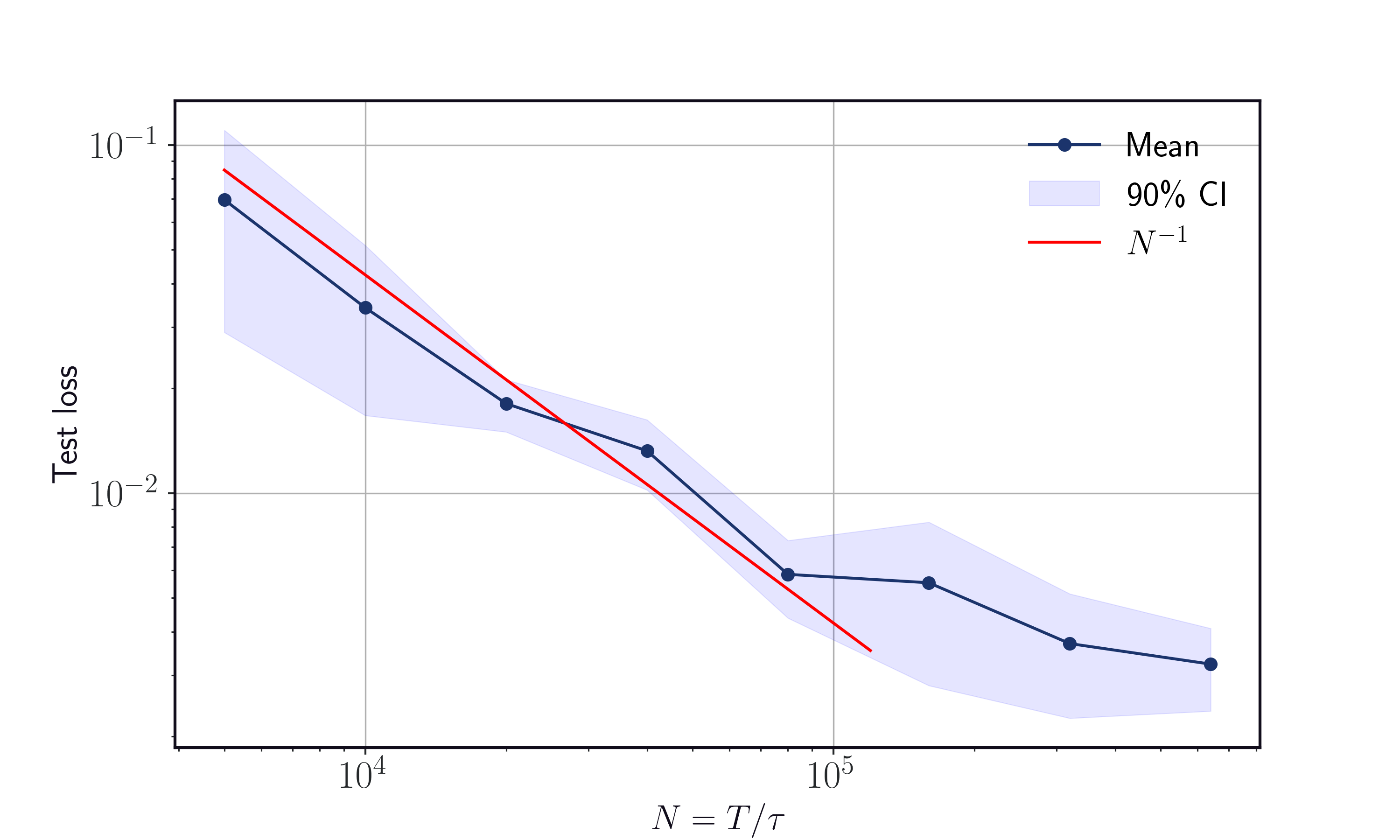
(a) $\tau=10^{-3}$ with varying $N$ and $T$

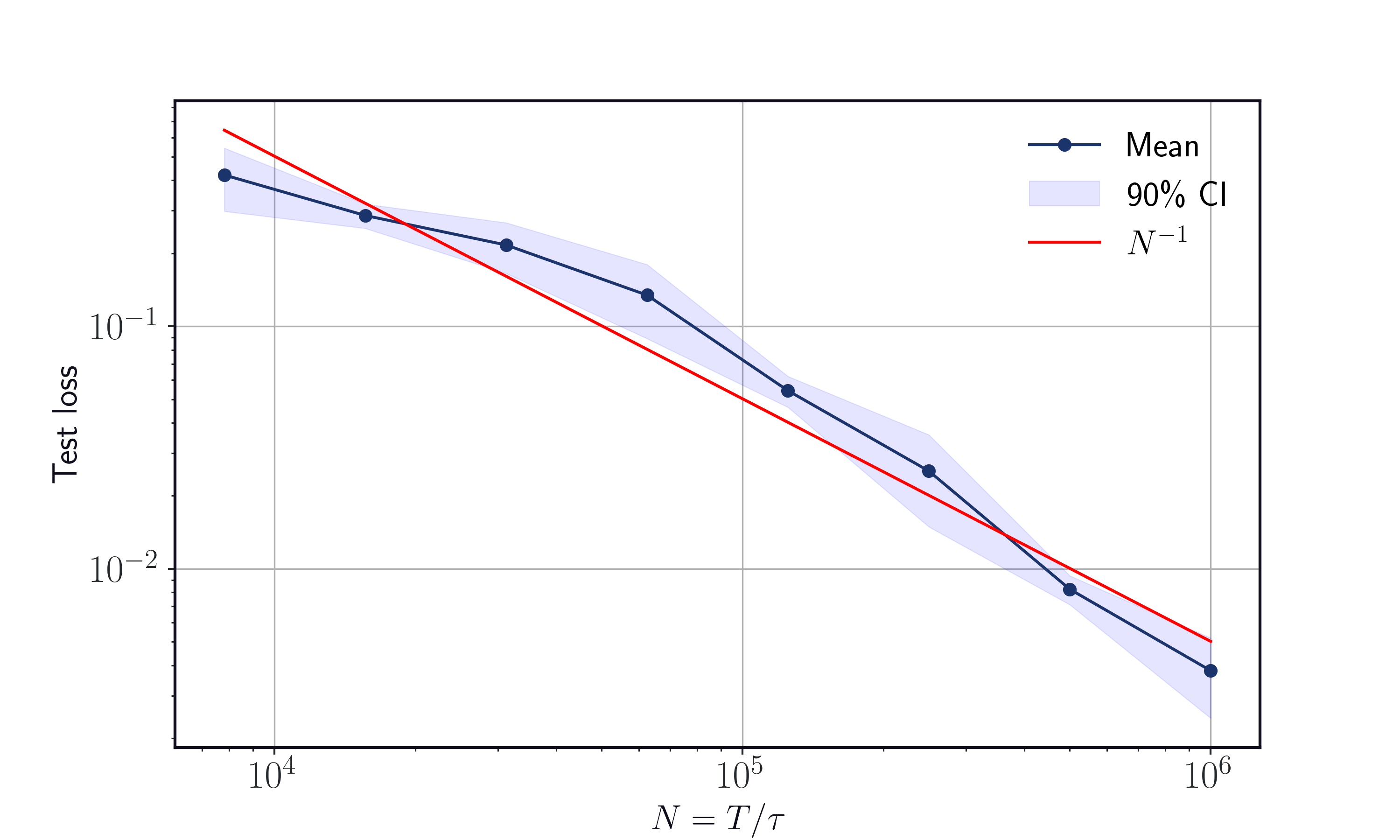
(b) $T=10^{3}$ with varying $N$ and $\tau$

Figure 1: Numerical results of the proposed neural diffusion estimator are consistent with the scaling expected from the theoretical bound. We probe this by varying $N$ and $T=N\tau$ with fixed lag time $\tau$ and also by varying $N$ and $\tau=T/N$ with fixed time horizon $T$.

4 Experiments

In this section, we present numerical results on a two-dimensional example, to illustrate the accordance between our theoretical convergence rates and those of our proposed neural diffusion estimator. Consider the following SDE in $\mathbb{R}^{2}$:

$$\mathrm{d}\boldsymbol{x}_{t}=f(\boldsymbol{x}_{t})\nabla f(\boldsymbol{x}_{t})\mathrm{d}t+f(\boldsymbol{x}_{t})\mathrm{d}\boldsymbol{w}_{t},$$ (14)

where

$$f(\boldsymbol{x})=1+\frac{1}{2}\cos(2\pi(x_{1}+x_{2})),$$

i.e. $\boldsymbol{b}(\boldsymbol{x})=f(\boldsymbol{x})\nabla f(\boldsymbol{x})$ and $D(\boldsymbol{x})=\frac{f(\boldsymbol{x})^{2}}{2}I$, where $I$ is the $2\times 2$ identity matrix. Then it is straightforward to verify that this diffusion process satisfies Assumption 2a, 2b, and 2c with smoothness $s=\infty$. Our goal is to estimate the value of the function $f(\boldsymbol{x})$ within $\Omega=[0,1)^{2}$. We employ Algorithm 1 for estimating both $\boldsymbol{b}(\boldsymbol{x})$ and $D(\boldsymbol{x})$ with separate neural networks and treat them entirely independently in the inference task. One may also prove that the stationary distribution $\widetilde{\Pi}$ of this diffusion process is given by the Lebesgue measure on the two-dimensional torus, which makes evaluating errors easier and more precise.

To impose the periodic boundary, we introduce an explicit regularization term to our training loss

$$\mathcal{L}_{\rm per}(\hat{g})=\mathbb{E}_{(\boldsymbol{x},\boldsymbol{y})\sim\mathrm{Unif}(\partial\Omega^{2}),\widetilde{\boldsymbol{x}}=\widetilde{\boldsymbol{y}}}\left[\left(\hat{g}(\boldsymbol{x})-\hat{g}(\boldsymbol{y})\right)^{2}\right],$$

approximated by $\hat{\mathcal{L}}_{\rm per}(\hat{g})$ with 1000 pairs of random samples empirically. The final training loss is thus $\tilde{\mathcal{L}}^{N}(\hat{g})+\lambda\hat{\mathcal{L}}_{\rm per}(\hat{g})$, where $\lambda$ is a hyperparameter and $\hat{g}$ can be either $\hat{\boldsymbol{b}}$ or $\hat{D}$.

We first generate data using the Euler-Maruyama method with a time step $\tau_{0}=2\times 10^{-5}$ up to $T_{0}=10^{4}$, and then sub-sample data at varying time steps $\tau$ and time horizons $T$ for each experiment instance from this common trajectory. We use a ResNet as our neural network structure with two residual blocks, each containing a fully-connected layer with a hidden dimension of 1000. Test data are generated by randomly selecting $5\times 10^{4}$ samples from another sufficiently long trajectory, which are shared by all experiment instances. The training process is executed on one Tesla V100 GPU.

According to our theoretical result (Theorem 9), the convergence rate of this implementation should be approximately of order $N^{-1}+\tau+T^{-1}$ up to $\log$ terms. We thus consider two schemes in our experiment. The first involves a fixed time step $\tau=10^{-3}$ with an expected rate of $\tau+N^{-1}$, and the other maintains a fixed $T=10^{3}$ with an expected rate of $N^{-1}+T^{-1}$. Each of the aforementioned instances is carried out five times. Figure 1 presents the mean values along with their corresponding confidence intervals from these runs. Additionally, reference lines indicating the expected convergence rate $N^{-1}$ are shown in red. Both schemes roughly exhibit the exponential decay phenomenon, aligning with our theoretical expectations. As depicted in Figure 1(a), the decreasing rate of the test error decelerates as $N$ exceeds a certain threshold. This can be attributed to the fact that when $N$ and $T$ are sufficiently large, the bias term $\tau$ arising from the discretization becomes the dominant factor in the error.

5 Conclusion

The ubiquity of correlated data in processes modeled with spatially-inhomogeneous diffusions has created substantial barriers to analysis. In this paper, we construct and analyze a neural network-based numerical algorithm for estimating multidimensional spatially-inhomogeneous diffusion processes based on discretely-observed data obtained from a single trajectory. Utilizing $\upbeta$-mixing conditions and local Rademacher complexity arguments, we establish the convergence rate for our neural diffusion estimator. Our upper bound has recovered the minimax optimal nonparametric function estimation rate in the common i.i.d. setting, even with correlated data. We expect our proof techniques serve as a model for general exponential ergodic diffusion processes beyond the toroidal setting considered here. Numerical experiments validate our theoretical findings and demonstrate the potential of applying the neural diffusion estimators across various contexts with provable accuracy guarantees. Extending our results to typical biophysical settings, e.g. compact domains with reflective boundaries and motion blur due to measurement error, could help establish more rigorous error estimates for physical inference problems.

Appendix A Detailed Proofs of Section 3.4

Besides $\hat{\mathcal{L}}_{N}^{g^{0}}(\hat{g})$ defined in the main text, we will use the following notation to denote the empirical loss over a sample set $S$ another than the sequence $S^{N}=(\boldsymbol{x}_{k\tau})_{k=0}^{N}$,

$$\hat{\mathcal{L}}_{|S|}^{g^{0}}(\hat{g};S):=\dfrac{1}{|S|}\sum_{X_{k}\in S}\left(g^{0}(\widetilde{X}_{k})-\hat{g}(\widetilde{X}_{k})\right)^{2},$$

where applying $\widetilde{\cdot}$ is to make sure each $\widetilde{X}_{k}\in\widetilde{\Omega}$. We will denote the squared loss $(g-g^{0})^{2}$ by $\ell\circ g$, and adopt the shorthand notation $f_{k\tau}=f(\widetilde{\boldsymbol{x}}(k\tau))$ for any function $f:\mathbb{R}^{d}\to\mathbb{R}$ throughout this section for simplicity, when the sequence $S^{N}=(\boldsymbol{x}_{k\tau})_{k=0}^{N}$ is clear from the context.

A.1 Proof of Theorem 6

In the following, we use $\widetilde{S}^{n}_{\widetilde{\Pi}}$ to denote a sample set consisting of $n$ i.i.d. samples drawn from the distribution $\widetilde{\Pi}$, i.e. $\widetilde{S}^{n}_{\widetilde{\Pi}}=\{\widetilde{X}_{1},\widetilde{X}_{2},\cdots,\widetilde{X}_{n}\}\sim{\widetilde{\Pi}}^{\otimes n}$.

To achieve the fast-rate generalization bound, we will make use of the following local Rademacher complexity argument:

Lemma 9 ((Bartlett, Bousquet, and Mendelson 2005, Theorem 3.3)).

Let $\mathfrak{F}$ be a function class and for each $f\in\mathfrak{F}$, $M_{1}\leq f\leq M_{2}$ and $\mathrm{Var}_{\widetilde{\Pi}}[f]\leq B\mathbb{E}_{\widetilde{\Pi}}[f]$ hold. Suppose $\mathfrak{R}_{N}(\{f\in\mathfrak{F}|\mathbb{E}_{\widetilde{\Pi}}[f]\leq r\})\leq\phi(r)$, where $\phi(r)$ is a sub-root function with a fixed point $r^{*}$. Then with probability at least $1-\delta$, we have for any $f\in\mathfrak{F}$

$$\mathbb{E}_{\widetilde{\Pi}}[f]\leq\dfrac{1}{1-\epsilon}\dfrac{1}{n}\sum_{\widetilde{X}_{k}\in\widetilde{S}_{\widetilde{\Pi}}^{n}}f(\widetilde{X}_{k})+\dfrac{704}{B\epsilon}r^{*}+\dfrac{\left(11(M_{2}-M_{1})\epsilon+26B\right)\log\frac{1}{\delta}}{\epsilon n}.$$

Remark 6.

Compared with Rademacher complexity, the arguments of local Rademacher complexity enables adaptation to the local quadratic geometry of the loss function and recovers the fast rate generalization bound (Bartlett, Bousquet, and Mendelson 2005). One of our contributions is showing how to adapt the local Rademacher arguments to the non-i.i.d data along the diffusion process and providing near-optimal bounds for diffusion estimation.

For completeness, we also provide the proof of Lemma 5:

Proof of Lemma 5.

Notice that each sub-sequence $S^{n}_{(a)}=(\boldsymbol{x}_{(kl+a)})_{k=0}^{n-1}$ is a sequence separated with time interval $l\tau$. Then the result follows directly from (Kuznetsov and Mohri 2017, Proposition 2) by setting the distribution $\Pi$ and sub-sample $\boldsymbol{Z}^{(j)}$ as $\widetilde{\Pi}$ and $S^{n}_{(a)}$, respectively. ∎

Remark 7.

Lemma 5 serves as a crucial tool for addressing the challenges presented by non-i.i.d. data points. To give an intuitive explanation, consider the way we segment the initial observations, represented by $S^{N}=(\boldsymbol{x}_{k\tau})_{k=0}^{N}$. We divide them into $l$ sub-sequences, denoted as $S^{n}_{(a)}=(\boldsymbol{x}_{(kl+a)\tau})_{k=0}^{n-1}$, for $a=0,\cdots,l-1$. In each of these sub-sequences, the observational gaps are $l\tau$, in contrast to the $\tau$ gap found in the initial sequence. By employing $\upbeta$-mixing and strategically choosing a sufficiently large value for $l$, we can effectively treat each sub-sequence as though it follows an i.i.d. distribution. The accuracy of this approximation is then determined by the mixing coefficient, as quantified in Lemma 5. With this setup, we can apply local Rademacher arguments to the approximated i.i.d. sequences, paving the way for fast convergence rates.

With Lemma 5 and Lemma 9, we are ready to present the proof of Theorem 6.

Proof of Theorem 6.

First, it is straightforward to check by Assumption 2b that for any $\widetilde{\boldsymbol{x}}\in\widetilde{\Omega}$,

$$|\ell\circ g^{*}(\widetilde{\boldsymbol{x}})-\mathbb{E}_{\widetilde{\Pi}}[\ell\circ g^{*}(\widetilde{\boldsymbol{x}})]|\leq 4M^{2},$$ (15)

and

$$\mathrm{Var}_{\widetilde{\Pi}}\left[\ell\circ g^{*}\right]\leq\mathbb{E}_{\widetilde{\Pi}}\left[\left(\ell\circ g^{*}\right)^{2}\right]=\mathbb{E}_{\widetilde{\Pi}}\left[\left(g^{*}-g^{0}\right)^{4}\right]\leq 4M^{2}\mathbb{E}_{\widetilde{\Pi}}[\ell\circ g^{*}],$$ (16)

Applying Lemma 9 for $f=\ell\circ\hat{g}$ with $B=4M^{2}$, $M_{1}=0$, and $M_{2}=4M^{2}$, yields that with probability at least $1-\delta^{\prime}/l$, we have

$$\mathcal{L}_{\widetilde{\Pi}}^{g^{0}}(\hat{g})\leq\dfrac{1}{1-\epsilon}\hat{\mathcal{L}}_{n}^{g^{0}}(\hat{g};\widetilde{S}^{n}_{\widetilde{\Pi}})+\dfrac{176}{M^{2}\epsilon}r^{*}+\dfrac{\left(44+\frac{104}{\epsilon}\right)M^{2}\log\left(\frac{l}{\delta^{\prime}}\right)}{n}.$$

Now we split the empirical loss $\hat{\mathcal{L}}_{N}^{g^{0}}(\hat{g})$ into the mean of $l$ empirical losses $\hat{\mathcal{L}}_{N}^{g^{0}}(\hat{g};S^{n}_{(a)})$, where $S^{n}_{(a)}$ are the sub-sequences of $S^{N}=(\boldsymbol{x}_{k\tau})_{k=0}^{N}$ obtained by sub-sampling:

$$\mathcal{L}_{\widetilde{\Pi}}^{g^{0}}(\hat{g})-\dfrac{1}{1-\epsilon}\hat{\mathcal{L}}_{N}^{g^{0}}(\hat{g}) =\dfrac{1}{N}\sum_{k=0}^{N-1}\left(\mathcal{L}_{\widetilde{\Pi}}^{g^{0}}(\hat{g})-\dfrac{1}{1-\epsilon}\ell\circ\hat{g}(\widetilde{\boldsymbol{x}}_{k\tau})\right)$$

$$=\dfrac{1}{l}\sum_{a=0}^{l-1}\left(\mathcal{L}_{\widetilde{\Pi}}^{g^{0}}(\hat{g})-\dfrac{1}{1-\epsilon}\dfrac{1}{n}\sum_{k=0}^{n-1}\ell\circ\hat{g}(\widetilde{\boldsymbol{x}}_{(kl+a)\tau})\right)$$

$$=\dfrac{1}{l}\sum_{a=0}^{l-1}\left(\mathcal{L}_{\widetilde{\Pi}}^{g^{0}}(\hat{g})-\dfrac{1}{1-\epsilon}\hat{\mathcal{L}}_{n}^{g^{0}}(\hat{g};S^{n}_{(a)})\right),$$

and for each summand, we apply Lemma 5 to the indicator function of the event $\left\{\mathcal{L}_{\widetilde{\Pi}}^{g^{0}}(\hat{g})-\frac{1}{1-\epsilon}\hat{\mathcal{L}}_{n}^{g^{0}}(\hat{g};S^{n}_{(a)})>\alpha\right\}$ and obtain

$$\mathbb{P}\left(\mathcal{L}_{\widetilde{\Pi}}^{g^{0}}(\hat{g})-\dfrac{1}{1-\epsilon}\hat{\mathcal{L}}_{n}^{g^{0}}(\hat{g};S^{n}_{(a)})>\alpha\right)\leq\mathbb{P}\left(\mathcal{L}_{\widetilde{\Pi}}^{g^{0}}(\hat{g})-\dfrac{1}{1-\epsilon}\hat{\mathcal{L}}_{n}^{g^{0}}(\hat{g};\widetilde{S}^{n}_{\widetilde{\Pi}})>\alpha\right)+n\upbeta(l\tau).$$

Then let $\alpha=\frac{176}{M^{2}\epsilon}r^{*}+\frac{\left(44+\frac{104}{\epsilon}\right)M^{2}\log\left(\frac{l}{\delta^{\prime}}\right)}{n}$, we have by the union bound

$$\mathbb{P}\left(\mathcal{L}_{\widetilde{\Pi}}^{g^{0}}(\hat{g})-\dfrac{1}{1-\epsilon}\hat{\mathcal{L}}_{N}^{g^{0}}(\hat{g})>\alpha\right) \leq\mathbb{P}\left(\dfrac{1}{l}\sum_{a=0}^{l-1}\left(\mathcal{L}_{\widetilde{\Pi}}^{g^{0}}(\hat{g})-\dfrac{1}{1-\epsilon}\hat{\mathcal{L}}_{n}^{g^{0}}(\hat{g};S^{n}_{(a)})\right)>\alpha\right)$$

$$\leq\sum_{a=0}^{l-1}\left(\mathbb{P}\left(\mathcal{L}_{\widetilde{\Pi}}^{g^{0}}(\hat{g})-\dfrac{1}{1-\epsilon}\hat{\mathcal{L}}_{n}^{g^{0}}(\hat{g};S^{n}_{(a)})>\alpha\right)\right)$$

$$\leq\sum_{a=0}^{l-1}\left(\mathbb{P}\left(\mathcal{L}_{\widetilde{\Pi}}^{g^{0}}(\hat{g})-\dfrac{1}{1-\epsilon}\hat{\mathcal{L}}_{n}^{g^{0}}(\hat{g};\widetilde{S}^{n}_{\widetilde{\Pi}})>\alpha\right)+n\upbeta(l\tau)\right)$$

$$\leq l\mathbb{P}\left(\mathcal{L}_{\widetilde{\Pi}}^{g^{0}}(\hat{g})-\dfrac{1}{1-\epsilon}\hat{\mathcal{L}}_{N}^{g^{0}}(\hat{g};\widetilde{S}^{n}_{\widetilde{\Pi}})>\alpha\right)+N\upbeta(l\tau)$$

$$\leq\delta^{\prime}+N\upbeta(l\tau)=\delta,$$

and the result follows. ∎

A.2 Proof of Theorem 7

In this section, the expectiation $\mathbb{E}$ should be referred to as being taken over the sub-$\sigma$-algebra of $\mathcal{F}_{0}^{T}$ generated by the trajectory $(\boldsymbol{x}_{k\tau})_{k=0}^{N}$ from which $\hat{g}$ is constructed by minimizing over the estimate empirical loss $\tilde{\mathcal{L}}_{N}^{g^{0}}(\hat{g};(\boldsymbol{x}_{k\tau})_{k=0}^{N})$.

We first consider the following decomposition of the expectation of the empirical loss $\hat{\mathcal{L}}_{N}^{g^{0}}(\hat{g})$:

Lemma 10.

For an arbitrary $\bar{g}\in\mathfrak{G}$, we have

$$\mathbb{E}\left[\hat{\mathcal{L}}_{N}^{g^{0}}(\hat{g})\right]\leq\mathbb{E}\left[\hat{\mathcal{L}}_{N}^{g^{0}}(\bar{g})\right]+\dfrac{2}{N}\mathbb{E}\left[\sum_{k=0}^{N-1}\Delta A_{k\tau}\left(\hat{g}_{k\tau}-\bar{g}_{k\tau}\right)\right]+\dfrac{2}{N}\mathbb{E}\left[\sum_{k=0}^{N-1}\Delta M_{k\tau}\left(\hat{g}_{k\tau}-g^{0}_{k\tau}\right)\right].$$ (17)

Proof.

By the definition of the estimator $\hat{g}$, we have $\tilde{\mathcal{L}}_{N}^{g^{0}}(\hat{g};(\boldsymbol{x}_{k\tau})_{k=0}^{N})\leq\tilde{\mathcal{L}}_{N}^{g^{0}}(\bar{g};(\boldsymbol{x}_{k\tau})_{k=0}^{N})$ for every possible sequence $(\boldsymbol{x}_{k\tau})_{k=0}^{N}$. Recall that

$$\tilde{\mathcal{L}}_{N}^{g^{0}}(g;(\boldsymbol{x}_{k\tau})_{k=0}^{N})=\dfrac{1}{N}\sum_{k=0}^{N-1}\left(g^{0}_{k\tau}+\Delta Z_{k\tau}-g_{k\tau}\right)^{2}=\hat{\mathcal{L}}_{N}^{g^{0}}(g)+\dfrac{2}{N}\sum_{k=0}^{N-1}\Delta Z_{k\tau}(g^{0}_{k\tau}-g_{k\tau})+\dfrac{1}{N}\sum_{k=0}^{N-1}(\Delta Z_{k\tau})^{2},$$

we have by taking expectation to both sides,

$$\mathbb{E}\left[\hat{\mathcal{L}}_{N}^{g^{0}}(\hat{g})\right]-\mathbb{E}\left[\hat{\mathcal{L}}_{N}^{g^{0}}(\bar{g})\right]$$

$$= \mathbb{E}\left[\tilde{\mathcal{L}}_{N}^{g^{0}}(\hat{g};(\boldsymbol{x}_{k\tau})_{k=0}^{N})\right]+\mathbb{E}\left[\dfrac{2}{N}\sum_{k=0}^{N-1}\Delta Z_{k\tau}\left(\hat{g}_{k\tau}-g^{0}_{k\tau}\right)\right]-\mathbb{E}\left[\dfrac{1}{N}\sum_{k=0}^{N-1}(\Delta Z_{k\tau})^{2}\right]$$

$$- \mathbb{E}\left[\tilde{\mathcal{L}}_{N}^{g^{0}}(\bar{g};(\boldsymbol{x}_{k\tau})_{k=0}^{N})\right]-\mathbb{E}\left[\dfrac{2}{N}\sum_{k=0}^{N-1}\Delta Z_{k\tau}\left(\bar{g}_{k\tau}-g^{0}_{k\tau}\right)\right]+\mathbb{E}\left[\dfrac{1}{N}\sum_{k=0}^{N-1}(\Delta Z_{k\tau})^{2}\right]$$

$$\leq \dfrac{2}{N}\mathbb{E}\left[\sum_{k=0}^{N-1}\Delta Z_{k\tau}\left(\hat{g}_{k\tau}-\bar{g}_{k\tau}\right)\right],$$

where we used the fact that the noise $(\Delta Z_{k\tau})_{k=0}^{N-1}$ only depends on the ground truth $g^{0}$ and the sequence $(\boldsymbol{x}_{k\tau})_{k=0}^{N}$.

Since $(M_{k\tau})_{k=0}^{N}$ forms a martingale, we have

$$\mathbb{E}\left[\sum_{k=0}^{N-1}\Delta M_{k\tau}\left(\bar{g}_{k\tau}-g^{0}_{k\tau}\right)\right]=\mathbb{E}\left[\sum_{k=0}^{N-1}\mathbb{E}\left[\Delta M_{k\tau}\left(\bar{g}_{k\tau}-g^{0}_{k\tau}\right)|\mathcal{F}_{0}^{k\tau}\right]\right]=0,$$

and thus

$$\mathbb{E}\left[\sum_{k=0}^{N-1}\Delta Z_{k\tau}\left(\hat{g}_{k\tau}-\bar{g}_{k\tau}\right)\right]$$

$$= \mathbb{E}\left[\sum_{k=0}^{N-1}\Delta A_{k\tau}\left(\hat{g}_{k\tau}-\bar{g}_{k\tau}\right)\right]+\mathbb{E}\left[\sum_{k=0}^{N-1}\Delta M_{k\tau}\left(\hat{g}_{k\tau}-\bar{g}_{k\tau}\right)\right]+\mathbb{E}\left[\sum_{k=0}^{N-1}\Delta M_{k\tau}\left(\bar{g}_{k\tau}-g^{0}_{k\tau}\right)\right]$$

$$= \mathbb{E}\left[\sum_{k=0}^{N-1}\Delta A_{k\tau}\left(\hat{g}_{k\tau}-\bar{g}_{k\tau}\right)\right]+\mathbb{E}\left[\sum_{k=0}^{N-1}\Delta M_{k\tau}\left(\hat{g}_{k\tau}-g^{0}_{k\tau}\right)\right],$$

and the result follows. ∎

Following Remark 5 in the main text, we will refer to the second term in the RHS of (17) as the bias term and the last as the martingale noise term.

For the bias term, we have the following simple bound:

Lemma 11.

For any $\epsilon>0$, we have

$$\mathbb{E}\left[\dfrac{1}{N}\sum_{k=0}^{N-1}\Delta A_{k\tau}\left(\hat{g}_{k\tau}-\bar{g}_{k\tau}\right)\right]\leq\dfrac{\epsilon}{4}\mathbb{E}\left[\hat{\mathcal{L}}_{N}^{g^{0}}(\hat{g})\right]+\dfrac{\epsilon}{2}\mathbb{E}\left[\hat{\mathcal{L}}_{N}^{g^{0}}(\bar{g})\right]+\dfrac{3}{2\epsilon}\mathbb{E}\left[\dfrac{1}{N}\sum_{k=0}^{N-1}(\Delta A_{k\tau})^{2}\right].$$

Proof.

$$\mathbb{E}\left[\dfrac{1}{N}\sum_{k=0}^{N-1}\Delta A_{k\tau}\left(\hat{g}_{k\tau}-\bar{g}_{k\tau}\right)\right]$$

$$= \mathbb{E}\left[\dfrac{1}{N}\sum_{k=0}^{N-1}\left(\Delta A_{k\tau}\left(\hat{g}_{k\tau}-g^{0}_{k\tau}\right)+\Delta A_{k\tau}\left(g^{0}_{k\tau}-\bar{g}_{k\tau}\right)\right)\right]$$

$$\leq \mathbb{E}\left[\dfrac{1}{N}\sum_{k=0}^{N-1}\left(\dfrac{1}{\epsilon}(\Delta A_{k\tau})^{2}+\dfrac{\epsilon}{4}\left(\hat{g}_{k\tau}-g^{0}_{k\tau}\right)^{2}+\dfrac{1}{2\epsilon}(\Delta A_{k\tau})^{2}+\dfrac{\epsilon}{2}\left(g^{0}_{k\tau}-\bar{g}_{k\tau}\right)^{2}\right)\right]$$

$$= \dfrac{\epsilon}{4}\mathbb{E}\left[\hat{\mathcal{L}}_{N}^{g^{0}}(\hat{g})\right]+\dfrac{\epsilon}{2}\mathbb{E}\left[\hat{\mathcal{L}}_{N}^{g^{0}}(\bar{g})\right]+\dfrac{3}{2\epsilon}\mathbb{E}\left[\dfrac{1}{N}\sum_{k=0}^{N-1}(\Delta A_{k\tau})^{2}\right],$$

where the inequality is by AM-GM and the last equality is due to Assumption 6. ∎

The following proof of the martingale noise term bound is inspired by the proof of (Schmidt-Hieber 2020, Lemma 4), where i.i.d. Gaussian noise is considered for nonparametric regression.

Definition 8 ($\epsilon$-covering).

We define the $\epsilon$-covering $\mathfrak{F}_{\epsilon}$ of a function class $\mathfrak{F}$ with respect to the norm $\|\cdot\|$ as the subset of $\mathfrak{F}$ with the smallest possible cardinality such that for any $f\in\mathfrak{F}$, there exists an $f^{\prime}\in\mathfrak{F}_{\epsilon}$ satisfying $\|f^{\prime}-f\|\leq\epsilon$. The cardinality of $\mathfrak{F}_{\epsilon}$ is denoted by $\mathcal{N}(\epsilon,\mathfrak{F},\|\cdot\|)$.

For a fixed $\rho>0$, let $\mathfrak{G}_{\rho}$ be the $\rho$-net of the function class $\mathfrak{G}$ with respect to the norm $\|\cdot\|_{\infty}$, where $\rho>0$. Without loss of generality, we assume that $\mathcal{N}(\rho,\mathfrak{G},\|\cdot\|_{\infty})\geq 2$.

We now introduce the following exponential inequality for local martingales.

Lemma 12.

Let $L_{t}$ be a continuous local martingale and $\left\langle L\right\rangle_{t}$ be the corresponding quadratic variation of $L_{t}$. If $\mathbb{E}\left[\sqrt{\langle L\rangle_{t}}\right]>0$, then for any $t,y>0$,

$$\mathbb{E}\left[\dfrac{y}{\sqrt{\langle L\rangle_{t}+y^{2}}}\exp\left(\frac{L_{t}^{2}}{2\left(\langle L\rangle_{t}+y^{2}\right)}\right)\right]\leq 1.$$

Moreover, then

$$\mathbb{E}\left[\exp\left(\dfrac{L_{t}^{2}}{4\left(\langle L\rangle_{t}+\mathbb{E}\left[\langle L\rangle_{t}\right]\right)}\right)\right]\leq\sqrt{2}.$$

Proof.

The result follows directly from (de la Peña, Klass, and Leung Lai 2004, Theorem 2.1) by setting $A=L_{t}$ and $B=\sqrt{\left\langle L\right\rangle_{t}}$, and noticing that

$$\mathbb{E}\left[\exp\left(\lambda L_{t}-\dfrac{\lambda^{2}}{2}\left\langle L\right\rangle_{t}\right)\right]\leq\mathbb{E}\left[\exp\left(\lambda L_{0}-\dfrac{\lambda^{2}}{2}\left\langle L\right\rangle_{0}\right)\right]=1$$

holds for any $t\geq 0$ and $\lambda\in\mathbb{R}$ by (de la Peña, Klass, and Leung Lai 2004, Lemma 1.2). Especially, the second inequality follows from

$$\mathbb{E}\left[\exp\left(\dfrac{L_{t}^{2}}{4\left(\langle L\rangle_{t}+\mathbb{E}\left[\langle L\rangle_{t}\right]\right)}\right)\right]\leq\mathbb{E}\left[\exp\left(\dfrac{L_{t}^{2}}{4\left(\langle L\rangle_{t}+\left(\mathbb{E}\left[\sqrt{\left\langle L\right\rangle_{t}}\right]\right)^{2}\right)}\right)\right]\leq\sqrt{2}.$$

∎

Lemma 12 enables us to give the following concentration inequality for the martingale noise term.

Lemma 13.

Let $g^{\prime}\in\mathfrak{G}_{\rho}$ such that $\|\hat{g}-g^{\prime}\|_{\infty}\leq\rho$, then for any $\epsilon>0$ and $g\in\mathfrak{G}_{\rho}$, we have

$$\mathbb{E}\left[\dfrac{1}{N}\sum_{k=0}^{N-1}\Delta M_{k\tau}\left(g^{\prime}_{k\tau}-g^{0}_{k\tau}\right)\right]\leq\dfrac{6\max_{k}\left|\mathbb{E}\left[\Delta\left\langle M\right\rangle_{k\tau}\big{|}\mathcal{F}_{0}^{k\tau}\right]\right|\log\mathcal{N}(\rho,\mathfrak{G},\|\cdot\|_{\infty})}{\epsilon N}+\dfrac{\epsilon}{4}\mathbb{E}\left[\hat{L}_{N}^{g^{0}}(g^{\prime})\right].$$ (18)

Proof.

First, for any $g\in\mathfrak{G}_{\rho}$, we define the following local martingale

$$L[g-g^{0}]_{t}=\sum_{k=0}^{N-1}(g_{k\tau}-g^{0}_{k\tau})\left(M_{t\wedge(k+1)\tau}-M_{t\wedge k\tau}\right),$$

for any $t\geq 0$ so that the LHS of (18) is $\frac{1}{N}\mathbb{E}\left[L[g-g^{0}]_{T}\right]$.

By martingale representation theorem, $(M_{t})_{t\geq 0}$ as a continuous local martingale is an Itô integral and thus the corresponding quadratic variation $(\left\langle M\right\rangle_{t})_{t\geq 0}$ exists. As a result, the quadratic variation of $L[g-g^{0}]$ is

$$\langle L[g-g^{0}]\rangle_{t}=\sum_{k=0}^{N-1}(g_{k\tau}-g^{0}_{k\tau})^{2}\left(\left\langle M\right\rangle_{t\wedge(k+1)\tau}-\left\langle M\right\rangle_{t\wedge k\tau}\right).$$

Take $y=\sqrt{\mathbb{E}\left[\left\langle L[g-g^{0}]\right\rangle_{T}\right]+\eta}$, where $\eta>0$, we have by Lemma 12,

$$\mathbb{E}\left[\dfrac{y}{\sqrt{\left\langle L[g-g^{0}]\right\rangle_{T}+y^{2}}}\exp\left(\dfrac{L[g-g^{0}]_{T}^{2}}{2\left(\left\langle L[g-g^{0}]\right\rangle_{T}+y^{2}\right)}\right)\right]\leq 1.$$

Therefore, by Jensen’s inequality and Cauchy-Schwarz, we have

$$\exp\mathbb{E}\left[\dfrac{L[g^{\prime}-g^{0}]_{T}^{2}}{4\left(\left\langle L[g^{\prime}-g^{0}]\right\rangle_{T}+y^{2}\right)}\right]\leq\mathbb{E}\left[\exp\left(\dfrac{L[g^{\prime}-g^{0}]_{T}^{2}}{4\left(\left\langle L[g^{\prime}-g^{0}]\right\rangle_{T}+y^{2}\right)}\right)\right]$$

$$\leq \sqrt{\mathbb{E}\left[\dfrac{y}{\sqrt{\left\langle L[g^{\prime}-g^{0}]\right\rangle_{T}+y^{2}}}\exp\left(\dfrac{L[g^{\prime}-g^{0}]_{T}^{2}}{2\left(\left\langle L[g^{\prime}-g^{0}]\right\rangle_{T}+y^{2}\right)}\right)\right]\mathbb{E}\left[\dfrac{\sqrt{\left\langle L[g^{\prime}-g^{0}]\right\rangle_{T}+y^{2}}}{y}\right]}$$

$$\leq \sqrt{\sum_{g\in\mathfrak{G}_{\rho}}\mathbb{E}\left[\dfrac{y}{\sqrt{\left\langle L[g-g^{0}]\right\rangle_{T}+y^{2}}}\exp\left(\dfrac{L[g-g^{0}]_{T}^{2}}{2\left(\left\langle L[g-g^{0}]\right\rangle_{T}+y^{2}\right)}\right)\right]\mathbb{E}\left[\dfrac{\sqrt{2y^{2}-\eta}}{y}\right]}$$

$$\leq \sqrt{\mathcal{N}(\rho,\mathfrak{G},\|\cdot\|_{\infty})\sqrt{2}},$$

where the second to last inequality is due to the fact $g^{\prime}\in\mathfrak{G}_{\rho}$ and thus the first expectation must be bounded by the summation over all possible $g\in\mathfrak{G}_{\rho}$.

Again by Cauchy-Schwarz,

$$\dfrac{1}{N}\mathbb{E}\left[L[g^{\prime}-g^{0}]_{T}\right] =\dfrac{1}{N}\mathbb{E}\left[\dfrac{L[g^{\prime}-g^{0}]_{T}}{2\sqrt{\left\langle L[g^{\prime}-g^{0}]\right\rangle_{T}+y^{2}}}2\sqrt{\left\langle L[g^{\prime}-g^{0}]\right\rangle_{T}+y^{2}}\right]$$

$$\leq\sqrt{\dfrac{4}{N^{2}}\mathbb{E}\left[\dfrac{L[g^{\prime}-g^{0}]_{T}^{2}}{4\left(\left\langle L[g^{\prime}-g^{0}]\right\rangle_{T}+y^{2}\right)}\right]\mathbb{E}\left[\left\langle L[g^{\prime}-g^{0}]\right\rangle_{T}+y^{2}\right]}$$

$$\leq\sqrt{\dfrac{2\log\mathcal{N}(\rho,\mathfrak{G},\|\cdot\|_{\infty})+\log 2}{N^{2}}\mathbb{E}\left[2\sum_{k=0}^{N-1}\left(g^{\prime}_{k\tau}-g^{0}_{k\tau}\right)^{2}\Delta\left\langle M\right\rangle_{k\tau}+\eta\right]}.$$

Finally, let $\eta\to 0$,

$$\dfrac{1}{N}\mathbb{E}\left[L[g^{\prime}-g^{0}]_{T}\right] \leq\sqrt{\dfrac{3\log\mathcal{N}(\rho,\mathfrak{G},\|\cdot\|_{\infty})}{N^{2}}2\mathbb{E}\left[\sum_{k=0}^{N-1}\left(g^{\prime}_{k\tau}-g^{0}_{k\tau}\right)^{2}\Delta\left\langle M\right\rangle_{k\tau}\right]}$$

$$\leq\sqrt{\dfrac{6\log\mathcal{N}(\rho,\mathfrak{G},\|\cdot\|_{\infty})}{N}\max_{k}\left|\mathbb{E}\left[\Delta\left\langle M\right\rangle_{k\tau}\big{|}\mathcal{F}_{0}^{k\tau}\right]\right|\mathbb{E}\left[\dfrac{1}{N}\sum_{k=0}^{N-1}\left(g^{\prime}_{k\tau}-g^{0}_{k\tau}\right)^{2}\right]}$$

$$\leq\dfrac{6\max_{k}\left|\mathbb{E}\left[\Delta\left\langle M\right\rangle_{k\tau}\big{|}\mathcal{F}_{0}^{k\tau}\right]\right|\log\mathcal{N}(\rho,\mathfrak{G},\|\cdot\|_{\infty})}{\epsilon N}+\dfrac{\epsilon}{4}\mathbb{E}\left[\hat{L}_{N}^{g^{0}}(g^{\prime})\right],$$

where the second inequality is due to the tower property

$$\mathbb{E}\left[\sum_{k=0}^{N-1}\left(g^{\prime}_{k\tau}-g^{0}_{k\tau}\right)^{2}\Delta\left\langle M\right\rangle_{k\tau}\right] =\sum_{k=0}^{N-1}\mathbb{E}\left[\left(g^{\prime}_{k\tau}-g^{0}_{k\tau}\right)^{2}\Delta\left\langle M\right\rangle_{k\tau}\right]$$ (19)

$$=\mathbb{E}\left[\sum_{k=0}^{N-1}\mathbb{E}\left[\left(g^{\prime}_{k\tau}-g^{0}_{k\tau}\right)^{2}\Delta\left\langle M\right\rangle_{k\tau}\big{|}\mathcal{F}_{0}^{k\tau}\right]\right]$$

$$=\mathbb{E}\left[\sum_{k=0}^{N-1}\left(g^{\prime}_{k\tau}-g^{0}_{k\tau}\right)^{2}\mathbb{E}\left[\Delta\left\langle M\right\rangle_{k\tau}\big{|}\mathcal{F}_{0}^{k\tau}\right]\right]$$

$$\leq\max_{k}\left|\mathbb{E}\left[\Delta\left\langle M\right\rangle_{k\tau}\big{|}\mathcal{F}_{0}^{k\tau}\right]\right|\mathbb{E}\left[\sum_{k=0}^{N-1}\left(g^{\prime}_{k\tau}-g^{0}_{k\tau}\right)^{2}\right]$$

and the last inequality is by AM-GM. ∎

It remains to bound the error by projecting the estimator $\hat{g}$ to the $\rho$-covering $\mathfrak{G}_{\rho}$, which is given by the following lemma.

Lemma 14.

Let $g^{\prime}\in\mathfrak{G}_{\rho}$ such that $\|\hat{g}-g^{\prime}\|_{\infty}\leq\rho$, then

$$\mathbb{E}\left[\dfrac{1}{N}\sum_{k=0}^{N-1}\Delta M_{k\tau}\left(\hat{g}_{k\tau}-g^{\prime}_{k\tau}\right)\right]\leq\sqrt{\dfrac{4\max_{k}\left|\mathbb{E}\left[\Delta\left\langle M\right\rangle_{k\tau}\big{|}\mathcal{F}_{0}^{k\tau}\right]\right|\rho^{2}\log 2}{N}}.$$

Proof.

We will follow the notations in the proof of Lemma 18. If $\left\langle L[\hat{g}-g^{\prime}]\right\rangle_{T}=0$, $L[\hat{g}-g^{\prime}]_{t}=0$ almost everywhere and the result holds trivially.

Now suppose $\left\langle L[\hat{g}-g^{\prime}]\right\rangle_{T}>0$, applying Lemma 12 and Jensen’s inequality yields

$$\mathbb{E}\left[\left(\dfrac{L[\hat{g}-g^{\prime}]_{T}^{2}}{4\left(\left\langle L[\hat{g}-g^{\prime}]\right\rangle_{T}+\mathbb{E}\left[\left\langle L[\hat{g}-g^{\prime}]\right\rangle_{T}\right]\right)}\right)\right]$$

$$\leq \log\mathbb{E}\left[\exp\left(\dfrac{L[\hat{g}-g^{\prime}]_{T}^{2}}{4\left(\left\langle L[\hat{g}-g^{\prime}]\right\rangle_{T}+\mathbb{E}\left[\left\langle L[\hat{g}-g^{\prime}]\right\rangle_{T}\right]\right)}\right)\right]\leq\dfrac{\log 2}{2}.$$

With a similar argument as in (19), we have

$$\mathbb{E}\left[\left\langle L[\hat{g}-g^{\prime}]\right\rangle_{T}\right]=\mathbb{E}\left[\sum_{k=0}^{N-1}\left(\hat{g}_{k\tau}-g^{\prime}_{k\tau}\right)^{2}\Delta\left\langle M\right\rangle_{k\tau}\right]$$

$$\leq \max_{k}\left|\mathbb{E}\left[\Delta\left\langle M\right\rangle_{k\tau}\big{|}\mathcal{F}_{0}^{k\tau}\right]\right|\mathbb{E}\left[\sum_{k=0}^{N-1}\left(\hat{g}_{k\tau}-g^{\prime}_{k\tau}\right)^{2}\right]\leq N\max_{k}\left|\mathbb{E}\left[\Delta\left\langle M\right\rangle_{k\tau}\big{|}\mathcal{F}_{0}^{k\tau}\right]\right|\rho^{2}.$$

Therefore, we have

$$\dfrac{1}{N}\mathbb{E}\left[L[\hat{g}-g^{\prime}]_{T}\right] =\dfrac{1}{N}\mathbb{E}\left[\dfrac{L[\hat{g}-g^{\prime}]_{T}}{2\sqrt{\left\langle L[\hat{g}-g^{\prime}]\right\rangle_{T}+\mathbb{E}\left[\left\langle L[\hat{g}-g^{\prime}]\right\rangle_{T}\right]}}2\sqrt{\left\langle L[\hat{g}-g^{\prime}]\right\rangle_{T}+\mathbb{E}\left[\left\langle L[\hat{g}-g^{\prime}]\right\rangle_{T}\right]}\right]$$

$$\leq\dfrac{2}{N}\sqrt{\mathbb{E}\left[\dfrac{L[\hat{g}-g^{\prime}]_{T}^{2}}{4\left(\left\langle L[\hat{g}-g^{\prime}]\right\rangle_{T}+\mathbb{E}\left[\left\langle L[\hat{g}-g^{\prime}]\right\rangle_{T}\right]\right)}\right]2\mathbb{E}\left[\left\langle L[\hat{g}-g^{\prime}]\right\rangle_{T}\right]}$$

$$\leq\sqrt{\dfrac{4\max_{k}\left|\mathbb{E}\left[\Delta\left\langle M\right\rangle_{k\tau}\big{|}\mathcal{F}_{0}^{k\tau}\right]\right|\rho^{2}\log 2}{N}}.$$

∎

Now we are ready to present the proof of Theorem 7.

Proof of Theorem 7.

Plug Lemma 11, 18, and 14 into Lemma 17, we have

$$\mathbb{E}\left[\hat{\mathcal{L}}_{N}^{g^{0}}(\hat{g})\right]\leq \mathbb{E}\left[\hat{\mathcal{L}}_{N}^{g^{0}}(\bar{g})\right]+\dfrac{2}{N}\mathbb{E}\left[\sum_{k=0}^{N-1}\Delta A_{k\tau}\left(\hat{g}_{k\tau}-\bar{g}_{k\tau}\right)\right]+\dfrac{2}{N}\mathbb{E}\left[\sum_{k=0}^{N-1}\Delta M_{k\tau}\left(\hat{g}_{k\tau}-g^{0}_{k\tau}\right)\right]$$

$$\leq \mathbb{E}\left[\hat{\mathcal{L}}_{N}^{g^{0}}(\bar{g})\right]+\dfrac{2}{N}\mathbb{E}\left[\sum_{k=0}^{N-1}\Delta A_{k\tau}\left(\hat{g}_{k\tau}-\bar{g}_{k\tau}\right)\right]$$

$$+\dfrac{2}{N}\mathbb{E}\left[\sum_{k=0}^{N-1}\Delta M_{k\tau}\left(\hat{g}_{k\tau}-g^{\prime}_{k\tau}\right)\right]+\dfrac{2}{N}\mathbb{E}\left[\sum_{k=0}^{N-1}\Delta M_{k\tau}\left(g^{\prime}_{k\tau}-g^{0}_{k\tau}\right)\right]$$

$$\leq \mathbb{E}\left[\hat{\mathcal{L}}_{N}^{g^{0}}(\bar{g})\right]+\dfrac{\epsilon}{2}\mathbb{E}\left[\hat{\mathcal{L}}_{N}^{g^{0}}(\hat{g})\right]+\epsilon\mathbb{E}\left[\hat{\mathcal{L}}_{N}^{g^{0}}(\bar{g})\right]+\dfrac{3}{\epsilon}\mathbb{E}\left[\dfrac{1}{N}\sum_{k=0}^{N-1}(\Delta A_{k\tau})^{2}\right]$$

$$+\dfrac{12\max_{k}\left|\mathbb{E}\left[\Delta\left\langle M\right\rangle_{k\tau}\big{|}\mathcal{F}_{0}^{k\tau}\right]\right|\log\mathcal{N}(\rho,\mathfrak{G},\|\cdot\|_{\infty})}{\epsilon N}+\dfrac{\epsilon}{2}\hat{L}^{N}(g)$$

$$+2\sqrt{\dfrac{4\max_{k}\left|\mathbb{E}\left[\Delta\left\langle M\right\rangle_{k\tau}\big{|}\mathcal{F}_{0}^{k\tau}\right]\right|\rho^{2}\log 2}{N}}.$$

Then we rearrange the terms and take infimum over all $\bar{g},\in\mathfrak{G}$,

$$\mathbb{E}\left[\hat{\mathcal{L}}_{N}^{g^{0}}(\hat{g})\right]\leq\dfrac{1+\epsilon}{1-\epsilon}\inf_{\bar{g}\in\mathfrak{G}}\mathbb{E}\left[\hat{\mathcal{L}}_{N}^{g^{0}}(\bar{g})\right]+\dfrac{3}{\epsilon}\mathbb{E}\left[\dfrac{1}{N}\sum_{k=0}^{N-1}(\Delta A_{k\tau})^{2}\right]$$

$$+\dfrac{12\max_{k}\left|\mathbb{E}\left[\Delta\left\langle M\right\rangle_{k\tau}\big{|}\mathcal{F}_{0}^{k\tau}\right]\right|\log\mathcal{N}(\rho,\mathfrak{G},\|\cdot\|_{\infty})}{\epsilon N}+2\sqrt{\dfrac{4\max_{k}\left|\mathbb{E}\left[\Delta\left\langle M\right\rangle_{k\tau}\big{|}\mathcal{F}_{0}^{k\tau}\right]\right|\rho^{2}\log 2}{N}}$$

$$\leq\dfrac{1+\epsilon}{1-\epsilon}\inf_{\bar{g}\in\mathfrak{G}}\mathbb{E}\left[\hat{\mathcal{L}}_{N}^{g^{0}}(\bar{g})\right]+\dfrac{3C_{A}}{\epsilon}\tau+\dfrac{12C_{M}\log\mathcal{N}(\rho,\mathfrak{G},\|\cdot\|_{\infty})}{\epsilon N\tau^{\gamma}}+2\sqrt{\dfrac{4C_{M}\rho^{2}\log 2}{N\tau^{\gamma}}},$$

where the last inequality is by Assumption 6 and 7.

∎

A.3 Proof of Theorem 8

Before we present the proof, we introduce the following lemma concerning the complexity of the sparse neural network function class, which will serve as the fundamental building block of our proof via local Rademacher arguments.

Lemma 15 ($\log$-covering number of $\mathfrak{N}(L,\boldsymbol{p},S,M)$ (Schmidt-Hieber 2020, Lemma 5)).

$$\log\mathcal{N}(\rho,\mathfrak{N}(L,\boldsymbol{p},S,\infty),\|\cdot\|_{\infty})\leq(S+1)\log\left(2^{2L+5}\rho^{-1}(L+1)d^{2}(S+1)^{2L}\right).$$

In fact, the Rademacher complexity $\mathfrak{R}_{N}(\mathfrak{F})$ can be bounded by $\log$-covering number via the following lemma.

Lemma 16 (Localized Dudley’s theorem).

For any function class $\mathfrak{F}$,

$$\mathfrak{R}_{N}(\mathfrak{F})\leq\mathbb{E}_{\mu^{\otimes N}}\left[\inf_{\rho>0}\left(4\rho+12\int_{\rho}^{\infty}\sqrt{\dfrac{\log\mathcal{N}(u,\mathfrak{F},\|\cdot\|_{2,S})}{N}}\mathrm{d}u\right)\right],$$

where the expectation in the definition of $\mathfrak{R}_{N}(\mathfrak{F})$ is taken over a sample set $S$ of $N$ i.i.d. samples $X_{1},\cdots,X_{N}$ drawn from a distribution $\mu$, and $\|\cdot\|_{2,S}$ denotes the $L^{2}$ norm with respect to the empirical measure $\frac{1}{N}\sum_{i=1}^{N}\delta(x-X_{i})$.

The following lemma will also be used in the proof of Theorem 8.

Lemma 17 (Talagrand’s contraction lemma).

Let $\phi:\mathbb{R}\to\mathbb{R}$ be a $L$-Lipschitz continuous function and $\mathfrak{F}$ be a function class, then

$$\mathfrak{R}_{N}(\mathfrak{F})\leq L\mathfrak{R}_{N}(\phi\circ\mathfrak{F}),$$

where $\phi\circ\mathfrak{F}=\{\phi\circ f|f\in\mathfrak{F}\}$.

With all lemmas aforementioned, we first bound the local Rademacher complexity of the sparse neural network class $\mathfrak{N}(L,\boldsymbol{p},S,M)$.

Lemma 18 (Local Rademacher complexity of $\mathfrak{N}(L,\boldsymbol{p},S,M)$).

The local Rademacher complexity of the sparse neural network class $\mathfrak{N}(L,\boldsymbol{p},S,M)$

$$\mathfrak{R}_{N}(\{\ell\circ g|g\in\mathfrak{N}(L,\boldsymbol{p},S,M),\mathbb{E}_{\widetilde{\Pi}}[\ell\circ g]\leq r\})$$

as appeared in Theorem 6 is bounded by the sub-root function

$$\phi(r)\leq \dfrac{32M}{N}+96M\sqrt{\dfrac{r(S+1)\log\left(2^{2L+5}N(L+1)d^{2}(S+1)^{2L}\right)}{N}}$$

$$+\dfrac{2304M^{2}(S+1)\log\left(2^{2L+5}N(L+1)d^{2}(S+1)^{2L}\right)}{N},$$

with the fixed point $r^{*}$ bounded by

$$r^{*}\leq\dfrac{64M+18432M^{2}(S+1)\log\left(2^{2L+5}N(L+1)d^{2}(S+1)^{2L}\right)}{N}.$$

Proof.

First, by applying Talagrand’s contraction lemma with Assumption 2b, and the localized Dudley’s theorem, we have

$$\mathfrak{R}_{N}(\{\ell\circ g|g\in\mathfrak{N}(L,\boldsymbol{p},S,M),\mathbb{E}_{\widetilde{\Pi}}[\ell\circ g]\leq r\})$$ (20)

$$\leq 4M\mathfrak{R}_{N}\left(\left\{g-g^{0}\big{|}g\in\mathfrak{N}(L,\boldsymbol{p},S,M),\mathbb{E}_{\widetilde{\Pi}}[(g-g^{0})^{2}]\leq r\right\}\right)$$

$$\leq 4M\mathbb{E}_{\Pi^{\otimes N}}\left[\inf_{\rho>0}\left(4\rho+12\int_{\rho}^{\sqrt{\hat{r}}}\sqrt{\dfrac{\log\mathcal{N}\left(u,\left\{g-g^{0}\big{|}g\in\mathfrak{N}(L,\boldsymbol{p},S,M),\mathbb{E}_{\widetilde{\Pi}}[(g-g^{0})^{2}]\leq r\right\},\|\cdot\|_{2,S}\right)}{N}}\mathrm{d}u\right)\right],$$

where the empirical localization radius depending on the sample set $S\sim\Pi^{\otimes N}$ is defined as

$$\hat{r}:=\sup_{g\in\mathfrak{N}(L,\boldsymbol{p},S,M),\mathbb{E}_{\widetilde{\Pi}}\left[(g-g^{0})^{2}\right]\leq r}\|g-g^{0}\|_{2,S}^{2},$$

and the last inequality is due to the fact that whenever $u>\sqrt{\hat{r}}$, the $u$-covering number with respect to $\|\cdot\|_{2,S}$ is exactly 1 and the integrand thus vanishes.

By choosing $\rho=\frac{1}{N}$ on the RHS of (20), we have

$$\inf_{\rho>0}\left(4\rho+12\int_{\rho}^{\sqrt{\hat{r}}}\sqrt{\dfrac{\log\mathcal{N}\left(u,\left\{g-g^{0}\big{|}g\in\mathfrak{N}(L,\boldsymbol{p},S,M),\mathbb{E}_{\widetilde{\Pi}}[(g-g^{0})^{2}]\leq r\right\},\|\cdot\|_{2,S}\right)}{N}}\mathrm{d}u\right)$$

$$\leq \dfrac{4}{N}+12\int_{1/N}^{\sqrt{\hat{r}}}\sqrt{\dfrac{\log\mathcal{N}\left(u,\left\{g-g^{0}\big{|}g\in\mathfrak{N}(L,\boldsymbol{p},S,M),\mathbb{E}_{\widetilde{\Pi}}[(g-g^{0})^{2}]\leq r\right\},\|\cdot\|_{2,S}\right)}{N}}\mathrm{d}u$$

$$\leq \dfrac{4}{N}+12\int_{1/N}^{\sqrt{\hat{r}}}\sqrt{\dfrac{\log\mathcal{N}\left(u,\left\{g-g^{0}|g\in\mathfrak{N}(L,\boldsymbol{p},S,M)\right\},\|\cdot\|_{2,S}\right)}{N}}\mathrm{d}u$$

$$\leq \dfrac{4}{N}+12\int_{1/N}^{\sqrt{\hat{r}}}\sqrt{\dfrac{\log\mathcal{N}\left(u,\mathfrak{N}(L,\boldsymbol{p},S,M),\|\cdot\|_{\infty}\right)}{N}}\mathrm{d}u$$

$$\leq \dfrac{4}{N}+12\int_{1/N}^{\sqrt{\hat{r}}}\sqrt{\dfrac{(S+1)\log\left(2^{2L+5}u^{-1}(L+1)d^{2}(S+1)^{2L}\right)}{N}}\mathrm{d}u$$

$$\leq \dfrac{4}{N}+12\sqrt{\hat{r}}\sqrt{\dfrac{(S+1)\log\left(2^{2L+5}N(L+1)d^{2}(S+1)^{2L}\right)}{N}},$$

where the third inequality is because of $\|\cdot\|_{2,S}\leq\|\cdot\|_{\infty}$, and the second to last equality is by Lemma 15.

Now set

$$\phi(r)=4M\mathbb{E}_{\Pi^{\otimes N}}\left[\dfrac{4}{N}+12\sqrt{\hat{r}}\sqrt{\dfrac{(S+1)\log\left(2^{2L+5}N(L+1)d^{2}(S+1)^{2L}\right)}{N}}\right],$$ (21)

then

$$\mathfrak{R}_{N}\left(\left\{\ell\circ g|g\in\mathfrak{N}(L,\boldsymbol{p},S,M),\mathbb{E}_{\widetilde{\Pi}}[\ell\circ g]\leq r\right\}\right)\leq\phi(r)$$

following the reasoning above.

Now we turn to bound the empirical localization radius $\hat{r}$ again by the local Rademacher complexity.

$$\mathbb{E}_{\Pi^{\otimes N}}\left[\hat{r}\right] =\mathbb{E}_{\Pi^{\otimes N}}\left[\sup_{g\in\mathfrak{N}(L,\boldsymbol{p},S,M),\mathbb{E}_{\widetilde{\Pi}}\left[(g-g^{0})^{2}\right]\leq r}\|g-g^{0}\|_{2,S}^{2}\right]$$

$$=\mathbb{E}_{\Pi^{\otimes N}}\left[\sup_{g\in\mathfrak{N}(L,\boldsymbol{p},S,M),\mathbb{E}_{\widetilde{\Pi}}\left[(g-g^{0})^{2}\right]\leq r}\dfrac{1}{N}\sum_{i=1}^{N}\left(g(X_{i})-g^{0}(X_{i})\right)^{2}\right]$$

$$=\mathbb{E}_{\Pi^{\otimes N}}\left[\sup_{g\in\mathfrak{N}(L,\boldsymbol{p},S,M),\mathbb{E}_{\widetilde{\Pi}}\left[(g-g^{0})^{2}\right]\leq r}\dfrac{1}{N}\sum_{i=1}^{N}\left(\left(g(X_{i})-g^{0}(X_{i})\right)^{2}-\mathbb{E}_{\widetilde{\Pi}}\left[(g-g^{0})^{2}\right]\right)\right]+r$$

$$\leq 2\mathfrak{R}_{N}\left(\left\{(g-g^{0})^{2}|g\in\mathfrak{N}(L,\boldsymbol{p},S,M),\mathbb{E}_{\widetilde{\Pi}}[(g-g^{0})^{2}]\leq r\right\}\right)+r\leq 2\phi(r)+r,$$

where the last inequality is by symmetrization (Boucheron, Lugosi, and Massart 2013).

Then from (21), we have by Jensen’s inequality,

$$\phi(r)\leq 4M\left(\dfrac{4}{N}+12\sqrt{\mathbb{E}_{\Pi^{\otimes N}}\left[\hat{r}\right]}\sqrt{\dfrac{(S+1)\log\left(2^{2L+5}N(L+1)d^{2}(S+1)^{2L}\right)}{N}}\right)$$

$$\leq 4M\left(\dfrac{4}{N}+12\sqrt{2\phi(r)+r}\sqrt{\dfrac{(S+1)\log\left(2^{2L+5}N(L+1)d^{2}(S+1)^{2L}\right)}{N}}\right)$$

$$\leq 4M\left(\dfrac{4}{N}+12\left(\sqrt{r}+\sqrt{2\phi(r)}\right)\sqrt{\dfrac{(S+1)\log\left(2^{2L+5}N(L+1)d^{2}(S+1)^{2L}\right)}{N}}\right)$$

$$\leq \dfrac{16M}{N}+48M\sqrt{\dfrac{r(S+1)\log\left(2^{2L+5}N(L+1)d^{2}(S+1)^{2L}\right)}{N}}$$

$$+\dfrac{\phi(r)}{2}+\dfrac{2304M^{2}(S+1)\log\left(2^{2L+5}N(L+1)d^{2}(S+1)^{2L}\right)}{N},$$

from which we deduce that

$$\mathfrak{R}_{N}\left(\left\{\ell\circ g|g\in\mathfrak{N}(L,\boldsymbol{p},S,M),\mathbb{E}_{\widetilde{\Pi}}[\ell\circ g]\leq r\right\}\right)$$

$$\leq \phi(r)\leq\dfrac{32M}{N}+96M\sqrt{\dfrac{r(S+1)\log\left(2^{2L+5}N(L+1)d^{2}(S+1)^{2L}\right)}{N}}$$

$$\ \ \ \ \ \ \ \ \ \ +\dfrac{4608M^{2}(S+1)\log\left(2^{2L+5}N(L+1)d^{2}(S+1)^{2L}\right)}{N},$$

which is clearly a sub-root function. Furthermore, by direct calculation, the fixed point $r^{*}$ of $\phi(r)$ satisfies

$$r^{*}\leq\dfrac{64M+18432M^{2}(S+1)\log\left(2^{2L+5}N(L+1)d^{2}(S+1)^{2L}\right)}{N},$$

which concludes the proof. ∎

The following lemma describes the approximation capability of $\mathfrak{N}(L,\boldsymbol{p},S,\infty)$:

Lemma 19 (Approximation error of $\mathfrak{N}(L,\boldsymbol{p},S,\infty)$ (Schmidt-Hieber 2020, Theorem 5)).

For any $g\in\mathcal{C}^{s}(\Omega,M)$ and any integer $m\geq 1$ and $K\geq(s+1)^{d}\vee(M+1)e^{d}$, there exists $\bar{g}\in\mathfrak{N}(L,\boldsymbol{p},S,\infty)$, where

$$L =8+(m+5)(1+\lceil\log_{2}(d\vee s)\rceil)$$

$$\boldsymbol{p} =\left(d,6(d+\lceil s\rceil)K,\cdots,6(d+\lceil s\rceil)K,1\right)$$

$$S \leq 141(d+s+1)^{3+r}K(m+6),$$

such that

$$\|\bar{g}-g\|_{L^{\infty}(\Omega)}\leq(2M+1)(1+d^{2}+s^{2})6^{d}K2^{-m}+M3^{s}K^{-s/d}.$$

With all the above preparations, we are ready to prove Theorem 8.

Proof of Theorem 8.

Choose $m$ to be the smallest integer such that $K2^{-m}\leq K^{-s/d}$, i.e.

$$m=\left\lceil\frac{(1+s/d)\log K}{\log 2}\right\rceil\lesssim\log K,$$

by Lemma 19, for any $g\in\mathcal{C}^{s}(\Omega,M)$, there exists $\bar{g}\in\mathfrak{N}(L,\boldsymbol{p},S,\infty)$, where

$$L\lesssim\log K,\quad\|\boldsymbol{p}\|_{\infty}\lesssim K,\quad S\lesssim K\log K,\$$ (22)

such that

$$\|\bar{g}-g\|_{L^{\infty}(\Omega)}\lesssim K^{-s/d}.$$

Thus in Lemma 18, we have

$$r^{*}\lesssim \dfrac{M+M^{2}(K\log K+1)\left((2\log K+5)\log 2+\log N+\log(\log K+1)+2\log d+2\log K\log(K\log K+1)\right)}{N}$$

$$\lesssim \dfrac{K\log K(\log K\log(K\log K)+\log N)}{N}\lesssim\dfrac{K\log^{3}K+K\log K\log N}{N}.$$

In Theorem 6, we take $\delta^{\prime}=N\upbeta(l\tau)=N^{-\alpha}$ with an arbitrary $\alpha>0$, i.e.

$$l=\dfrac{\log M_{\widetilde{\Pi}}+(1+\alpha)\log N}{C_{\widetilde{\Pi}}\tau}\lesssim\dfrac{\log N}{\tau}.$$

Then with probability at least $1-2N^{-\alpha}$, we have

$$\mathcal{L}_{\widetilde{\Pi}}^{g^{0}}(\hat{g})\leq \dfrac{1}{1-\epsilon}\hat{\mathcal{L}}_{N}^{g^{0}}(\hat{g})+\dfrac{176}{M^{2}\epsilon}r^{*}+\dfrac{l\left(44\epsilon+104\right)M^{2}\log\left(lN^{\alpha}\right)}{\epsilon N}$$

$$\lesssim \hat{\mathcal{L}}_{N}^{g^{0}}(\hat{g})+\dfrac{K\log^{3}K+K\log K\log N}{N}+\dfrac{\log^{2}N}{N\tau}.$$

In Lemma 15, take $\rho=1/N$ and $L$, $\boldsymbol{p}$, and $S$ as in (22), we have

$$\log\mathcal{N}(\rho,\mathfrak{N}(L,\boldsymbol{p},S,\infty),\|\cdot\|_{\infty})\leq K\log^{3}K+K\log K\log N,$$

and thus in Theorem 7 with also $\rho=1/N$,

$$\mathbb{E}\left[\hat{\mathcal{L}}_{N}^{g^{0}}(\hat{g})\right]\lesssim \inf_{\hat{g}\in\mathfrak{G}}\mathbb{E}\left[\hat{\mathcal{L}}_{N}^{g^{0}}(\hat{g})\right]+\tau+\dfrac{\log\mathcal{N}(1/N,\mathfrak{N}(L,\boldsymbol{p},S,M),\|\cdot\|_{\infty})}{N\tau^{\gamma}}+\sqrt{\dfrac{\rho^{2}}{N\tau^{\gamma}}}$$

$$\lesssim \inf_{\hat{g}\in\mathfrak{G}}\|\hat{g}-g^{0}\|_{\infty}^{2}+\tau+\dfrac{\log\mathcal{N}(1/N,\mathfrak{N}(L,\boldsymbol{p},S,\infty),\|\cdot\|_{\infty})}{N\tau^{\gamma}}+\sqrt{\dfrac{1}{N^{3}\tau^{\gamma}}}$$

$$\lesssim K^{-2s/d}+\tau+\dfrac{K\log^{3}K+K\log K\log N}{N\tau^{\gamma}}+\dfrac{1}{N},$$

where we used $N\tau^{\gamma}\geq N\tau\geq 1$.

Finally, we conclude

$$\mathbb{E}\left[\mathcal{L}_{\widetilde{\Pi}}^{g^{0}}(\hat{g})\right]\lesssim \mathbb{E}\left[\hat{\mathcal{L}}_{N}^{g^{0}}(\hat{g})\right]+\dfrac{K\log^{3}K+K\log K\log N}{N}+\dfrac{\log^{2}N}{N\tau}$$

$$\lesssim K^{-2s/d}+\tau+\dfrac{K\log^{3}K+K\log K\log N}{N(\tau^{\gamma}\wedge 1)}+\dfrac{1}{N}+\dfrac{\log^{2}N}{N\tau}$$

$$\lesssim \left(N(\tau^{\gamma}\wedge 1)\right)^{-\frac{2s}{2s+d}}\log^{3}(N(\tau^{\gamma}\wedge 1))+\tau+\dfrac{\log^{2}N}{N\tau},$$

by taking $K\asymp(N(\tau^{\gamma}\wedge 1))^{\frac{d}{2s+d}}$.

∎

Appendix B Detailed Proofs of Section 3.3

In this section, we present the detailed proofs of the results in Section 3.3, including Theorem 3 and Theorem 9. Both proofs are based on Theorem 8 that we have proved in Appendix A. Specifically, we would like to verify the conditions of Theorem 8 for the drift and diffusion estimation problems, respectively. To this end, we first compute the noise $\Delta Z_{k\tau}$ of the drift and diffusion estimators as in (10), analyze its decomposition into the bias term $\Delta A_{k\tau}$ and the variance term $\Delta M_{k\tau}$, and then verify Assumption 6 and find the exponent $\gamma$ in Assumption 7 for both drift and diffusion estimators.

Lemma 20.

For $s\in[k\tau,(k+1)\tau]$,

$$\mathbb{E}\left[\|\boldsymbol{x}_{t}-\boldsymbol{x}_{k\tau}\|^{2}\mid\mathcal{F}_{0}^{k\tau}\right]\leq e^{\tau}(M^{2}d+2Md^{2})(t-k\tau).$$

Proof.

By Itô’s formula, we have for $s\in[k\tau,(k+1)\tau]$,

$$\mathrm{d}\|\boldsymbol{x}_{s}-\boldsymbol{x}_{k\tau}\|^{2} =2(\boldsymbol{x}_{s}-\boldsymbol{x}_{k\tau})^{\top}\mathrm{d}\boldsymbol{x}_{s}+d\mathrm{d}\langle\boldsymbol{x}_{s}-\boldsymbol{x}_{k\tau},\boldsymbol{x}_{s}-\boldsymbol{x}_{k\tau}\rangle$$

$$=2(\boldsymbol{x}_{s}-\boldsymbol{x}_{k\tau})^{\top}\left(\boldsymbol{b}_{s}\mathrm{d}s+\Sigma_{s}\mathrm{d}\boldsymbol{w}_{s}\right)+d\mathrm{d}\langle\boldsymbol{x}_{s}-\boldsymbol{x}_{k\tau},\boldsymbol{x}_{s}-\boldsymbol{x}_{k\tau}\rangle$$

$$=2(\boldsymbol{x}_{s}-\boldsymbol{x}_{k\tau})^{\top}\left(\boldsymbol{b}_{s}\mathrm{d}s+\Sigma_{s}\mathrm{d}\boldsymbol{w}_{s}\right)+d\mathrm{tr}\left(\Sigma_{s}^{\top}\Sigma_{s}\right)\mathrm{d}s$$

$$=\left(2(\boldsymbol{x}_{s}-\boldsymbol{x}_{k\tau})^{\top}\boldsymbol{b}_{s}+2d\mathrm{tr}D_{s}\right)\mathrm{d}s+2(\boldsymbol{x}_{s}-\boldsymbol{x}_{k\tau})^{\top}\Sigma_{s}\mathrm{d}\boldsymbol{w}_{s}.$$

Therefore for any $t\in[k\tau,(k+1)\tau]$,

$$\mathbb{E}\left[\|\boldsymbol{x}_{t}-\boldsymbol{x}_{k\tau}\|^{2}\mid\mathcal{F}_{0}^{k\tau}\right] =\mathbb{E}\left[\int_{k\tau}^{t}\left(2(\boldsymbol{x}_{s}-\boldsymbol{x}_{k\tau})^{\top}\boldsymbol{b}_{s}+2d\mathrm{tr}D_{s}\right)\mathrm{d}s\bigg{|}\mathcal{F}_{0}^{k\tau}\right]$$

$$\leq(M^{2}d+2Md)(t-k\tau)+\int_{k\tau}^{t}\mathbb{E}\left[\|\boldsymbol{x}_{s}-\boldsymbol{x}_{k\tau}\|^{2}\mid\mathcal{F}_{0}^{k\tau}\right]\mathrm{d}s,$$

and by Gronwall’s inequality, we have

$$\mathbb{E}\left[\|\boldsymbol{x}_{t}-\boldsymbol{x}_{k\tau}\|^{2}\mid\mathcal{F}_{0}^{k\tau}\right]\leq e^{\tau}(M^{2}d+2Md^{2})(t-k\tau).$$

∎

B.1 Proof of Theorem 3

As a warm-up for the proof of Theorem 9, we first prove the corresponding upper bound for drift estimation:

Proof of Theorem 3.

Suppose that $1\leq i\leq d$. Let $b^{i}_{t}$, the $i$-th component of the drift $\boldsymbol{b}_{t}$, be our target function $g^{0}$. We also use $Z^{i}_{t}$, $A^{i}_{t}$, and $M^{i}_{t}$ to denote the corresponding noise terms.

For any $0\leq k\leq N-1$, we have by Itô’s formula,

$$\dfrac{x^{i}_{(k+1)\tau}-x^{i}_{k\tau}}{\tau}=b^{i}_{k\tau}+\dfrac{1}{\tau}\int_{k\tau}^{(k+1)\tau}\left(b^{i}_{t}-b^{i}_{k\tau}\right)\mathrm{d}t+\dfrac{1}{\tau}\int_{k\tau}^{(k+1)\tau}\boldsymbol{\Sigma}_{t}^{i}\mathrm{d}\boldsymbol{w}_{t},$$

and compare the estimated empirical loss for drift inference (5) with the general form (10), we have

$$\Delta Z^{i}_{k\tau}=\dfrac{1}{\tau}\int_{k\tau}^{(k+1)\tau}\left(b^{i}_{t}-b^{i}_{k\tau}\right)\mathrm{d}t+\dfrac{1}{\tau}\int_{k\tau}^{(k+1)\tau}\boldsymbol{\Sigma}_{t}^{i}\mathrm{d}\boldsymbol{w}_{t}.$$

By definition, we also have

$$\Delta A^{i}_{k\tau}=\mathbb{E}\left[\dfrac{1}{\tau}\int_{k\tau}^{(k+1)\tau}\left(b^{i}_{t}-b^{i}_{k\tau}\right)\mathrm{d}t\right],\quad\Delta M^{i}_{k\tau}=\dfrac{1}{\tau}\int_{k\tau}^{(k+1)\tau}\boldsymbol{\Sigma}_{t}^{i}\mathrm{d}\boldsymbol{w}_{t}.$$

The following simple argument

$$\Delta\left\langle M^{i}\right\rangle_{k\tau}=\dfrac{1}{\tau^{2}}\int_{k\tau}^{(k+1)\tau}\|\boldsymbol{\Sigma}_{t}^{i}\|_{2}^{2}\mathrm{d}t\leq M^{2}d\tau^{-1}$$

validates Assumption 7 with $\gamma=1$.

Also, by Cauchy-Schwarz and Lemma 20, we have

$$\mathbb{E}\left[\left(\Delta A^{i}_{k\tau}\right)^{2}\big{|}\mathcal{F}_{0}^{k\tau}\right]\leq \mathbb{E}\left[\dfrac{1}{\tau^{2}}\left(\int_{k\tau}^{(k+1)\tau}\left(b^{i}_{t}-b^{i}_{k\tau}\right)\mathrm{d}t\right)^{2}\bigg{|}\mathcal{F}_{0}^{k\tau}\right]$$

$$\leq \mathbb{E}\left[\dfrac{1}{\tau}\int_{k\tau}^{(k+1)\tau}\left(b^{i}_{t}-b^{i}_{k\tau}\right)^{2}\mathrm{d}t\bigg{|}\mathcal{F}_{0}^{k\tau}\right]$$

$$\leq \mathbb{E}\left[\dfrac{M^{2}}{\tau}\int_{k\tau}^{(k+1)\tau}\left\|\boldsymbol{x}_{t}-\boldsymbol{x}_{k\tau}\right\|^{2}\mathrm{d}t\bigg{|}\mathcal{F}_{0}^{k\tau}\right]$$

$$\leq \dfrac{1}{\tau}\int_{k\tau}^{(k+1)\tau}e^{\tau}(M^{2}d+2Md^{2})(t-k\tau)\mathrm{d}t$$

$$\leq \dfrac{1}{2}e^{\tau}(M^{2}d+2Md^{2})\tau,$$

and Assumption 6 is thus satisfied.

Finally, we apply Theorem 8 to $g^{0}=b^{i}$, and obtain the final rate

$$\mathbb{E}\left[\hat{\mathcal{L}}_{N}^{g^{0}}(\hat{b^{i}})\right]\lesssim \left(N\tau\right)^{-\frac{2s}{2s+d}}\log^{3}(N\tau)+\tau+\dfrac{\log^{2}N}{N\tau}$$

$$\lesssim T^{-\frac{2s}{2s+d}}\log^{3}T+\tau,$$

and the proof is thus complete by repeating for all $1\leq i\leq d$. ∎

B.2 Proof of Theorem 9

The proof for diffusion estimation requires a even more delicate analysis on the dynamics of the SDE (1).

Proof of Theorem 9.

Following the notations introduced in the proof of Theorem 9, for $1\leq i,j\leq d$, let $D^{ij}$ be the target function and $Z^{ij}$, $A^{ij}$, $M^{ij}$ be the corresponding noise terms.

For any $0\leq k\leq N-1$, define the following auxiliary process for $s\in[0,\tau]$,

$$Y_{k,s}^{i}:=x^{i}_{k\tau+s}-x^{i}_{k\tau}-\hat{b}^{i}_{k\tau}s=\int_{k\tau}^{k\tau+s}\left(b^{i}_{t}-\hat{b}^{i}_{k\tau}\right)\mathrm{d}t+\int_{k\tau}^{k\tau+s}\boldsymbol{\Sigma}_{t}^{i}\mathrm{d}\boldsymbol{w}_{t},$$ (23)

where $\boldsymbol{\Sigma}^{i}$ denotes the $i$-th row of $\Sigma$ (a row vector). Plugging (23) into the estimated empirical loss for diffusion estimation (6), we have by definition

$$\Delta Z^{ij}_{k\tau} =(2\tau)^{-1}Y_{k,\tau}^{i}Y_{k,\tau}^{j}-D^{ij}_{k\tau}$$

$$\Delta A^{ij}_{k\tau} =(2\tau)^{-1}\mathbb{E}\left[Y_{k,\tau}^{i}Y_{k,\tau}^{j}\right]-D^{ij}_{k\tau}$$

$$\Delta\left\langle M^{ij}\right\rangle_{k\tau} =(2\tau)^{-2}\left\langle Y_{k}^{i}Y_{k}^{j}\right\rangle_{\tau}.$$

The process $Y_{k,s}^{i}$ satisfies the following SDE:

$$\mathrm{d}Y_{k,s}^{i}=\left(b_{k\tau+s}^{i}-\hat{b}_{k\tau}^{i}\right)\mathrm{d}s+\boldsymbol{\Sigma}_{k\tau+s}^{i}\mathrm{d}\boldsymbol{w}_{s}.$$

By Itô’s formula, the process $\left(Y_{k,s}^{i}Y_{k,s}^{j}\right)_{0\leq s\leq\tau}$ as the product of $Y_{k,s}^{i}$ and $Y_{k,s}^{j}$ also satisfies an SDE as follows:

$$\mathrm{d}\left(Y_{k,s}^{i}Y_{k,s}^{j}\right)=Y_{k,s}^{i}\mathrm{d}Y_{k,s}^{j}+Y_{k,s}^{j}\mathrm{d}Y_{k,s}^{i}+\mathrm{d}\left\langle Y_{k,s}^{i},Y_{k,s}^{j}\right\rangle$$

$$= \left[Y_{k,s}^{i}\left(b_{k\tau+s}^{j}-\hat{b}_{k\tau}^{j}\right)+Y_{k,s}^{j}\left(b_{k\tau+s}^{i}-\hat{b}_{k\tau}^{i}\right)+\boldsymbol{\Sigma}^{i}_{k\tau+s}\left(\boldsymbol{\Sigma}^{j}_{k\tau+s}\right)^{\top}\right]\mathrm{d}s+\left[Y_{k,s}^{i}\boldsymbol{\Sigma}_{k\tau+s}^{j}+Y_{k,s}^{j}\boldsymbol{\Sigma}_{k\tau+s}^{i}\right]\mathrm{d}\boldsymbol{w}_{s}$$

with its quadratic variation satisfying

$$\mathrm{d}\left\langle Y_{k}^{i}Y_{k}^{j}\right\rangle_{s}=\left|Y_{k,s}^{i}\boldsymbol{\Sigma}_{k\tau+s}^{j}+Y_{k,s}^{j}\boldsymbol{\Sigma}_{k\tau+s}^{i}\right|^{2}\mathrm{d}s.$$

By direct calculation, we have

$$\mathbb{E}\left[Y_{k,s}^{i}Y_{k,s}^{j}\big{|}\mathcal{F}_{0}^{k\tau}\right]$$ (24)

$$= \mathbb{E}\left[\int_{0}^{s}\left(\int_{0}^{s_{1}}\left(b_{k\tau+s_{2}}^{i}-\hat{b}_{k\tau}^{i}\right)\mathrm{d}s_{2}+\int_{0}^{s_{1}}\boldsymbol{\Sigma}_{k\tau+s_{2}}^{i}\mathrm{d}\boldsymbol{w}_{s_{2}}\right)\left(b_{k\tau+s_{1}}^{j}-\hat{b}_{k\tau}^{j}\right)\mathrm{d}s_{1}\bigg{|}\mathcal{F}_{0}^{k\tau}\right]$$

$$+ \mathbb{E}\left[\int_{0}^{s}\left(\int_{0}^{s_{2}}\left(b_{k\tau+s_{1}}^{j}-\hat{b}_{k\tau}^{j}\right)\mathrm{d}s_{1}+\int_{0}^{s_{2}}\boldsymbol{\Sigma}_{k\tau+s_{1}}^{j}\mathrm{d}\boldsymbol{w}_{s_{1}}\right)\left(b_{k\tau+s_{2}}^{i}-\hat{b}_{k\tau}^{i}\right)\mathrm{d}s_{2}\bigg{|}\mathcal{F}_{0}^{k\tau}\right]$$

$$+ \mathbb{E}\left[\int_{0}^{s}\boldsymbol{\Sigma}^{i}_{k\tau+s^{\prime}}\left(\boldsymbol{\Sigma}^{j}_{k\tau+s^{\prime}}-\boldsymbol{\Sigma}_{k\tau}^{j}\right)^{\top}+\left(\boldsymbol{\Sigma}^{i}_{k\tau+s^{\prime}}-\boldsymbol{\Sigma}^{i}_{k\tau}\right)\left(\boldsymbol{\Sigma}_{k\tau}^{j}\right)^{\top}\mathrm{d}s^{\prime}\bigg{|}\mathcal{F}_{0}^{k\tau}\right]+s\boldsymbol{\Sigma}_{k\tau}^{i}\left(\boldsymbol{\Sigma}_{k\tau}^{j}\right)^{\top}$$

$$= \int_{0}^{s}\int_{0}^{s}\mathbb{E}\left[\left(b_{k\tau+s_{1}}^{i}-\hat{b}_{k\tau}^{i}\right)\left(b_{k\tau+s_{2}}^{j}-\hat{b}_{k\tau}^{j}\right)\bigg{|}\mathcal{F}_{0}^{k\tau}\right]\mathrm{d}s_{1}\mathrm{d}s_{2}$$

$$+\mathbb{E}\left[\int_{0}^{s}\boldsymbol{\Sigma}^{i}_{k\tau+s^{\prime}}\left(\boldsymbol{\Sigma}^{j}_{k\tau+s^{\prime}}-\boldsymbol{\Sigma}_{k\tau}^{j}\right)^{\top}+\left(\boldsymbol{\Sigma}^{i}_{k\tau+s^{\prime}}-\boldsymbol{\Sigma}^{i}_{k\tau}\right)\left(\boldsymbol{\Sigma}_{k\tau}^{j}\right)^{\top}\mathrm{d}s^{\prime}\bigg{|}\mathcal{F}_{0}^{k\tau}\right]+2sD^{ij}_{k\tau}.$$

For the first term of (24), we have the following bound by applying Cauchy-Schwarz

$$\left(\int_{0}^{s}\int_{0}^{s}\mathbb{E}\left[\left(b_{k\tau+s_{1}}^{i}-\hat{b}_{k\tau}^{i}\right)\left(b_{k\tau+s_{2}}^{j}-\hat{b}_{k\tau}^{j}\right)\bigg{|}\mathcal{F}_{0}^{k\tau}\right]\mathrm{d}s_{1}\mathrm{d}s_{2}\right)^{2}$$

$$\lesssim \left(\int_{0}^{s}\int_{0}^{s}\mathbb{E}\left[\left(b_{k\tau+s_{1}}^{i}-b_{k\tau}^{i}\right)\left(b_{k\tau+s_{2}}^{j}-b_{k\tau}^{j}\right)\bigg{|}\mathcal{F}_{0}^{k\tau}\right]\mathrm{d}s_{1}\mathrm{d}s_{2}\right)^{2}$$

$$+ \left(\int_{0}^{s}\int_{0}^{s}\mathbb{E}\left[\left(b_{k\tau}^{i}-\hat{b}_{k\tau}^{i}\right)\left(b_{k\tau+s_{2}}^{j}-b_{k\tau}^{j}\right)\bigg{|}\mathcal{F}_{0}^{k\tau}\right]\mathrm{d}s_{1}\mathrm{d}s_{2}\right)^{2}$$

$$+ \left(\int_{0}^{s}\int_{0}^{s}\mathbb{E}\left[\left(b_{k\tau+s_{1}}^{i}-b_{k\tau}^{i}\right)\left(b_{k\tau}^{j}-\hat{b}_{k\tau}^{j}\right)\bigg{|}\mathcal{F}_{0}^{k\tau}\right]\mathrm{d}s_{1}\mathrm{d}s_{2}\right)^{2}$$

$$+ \left(\int_{0}^{s}\int_{0}^{s}\mathbb{E}\left[\left(b_{k\tau}^{i}-\hat{b}_{k\tau}^{i}\right)\left(b_{k\tau}^{j}-\hat{b}_{k\tau}^{j}\right)\bigg{|}\mathcal{F}_{0}^{k\tau}\right]\mathrm{d}s_{1}\mathrm{d}s_{2}\right)^{2}$$

$$\lesssim s^{2}\int_{0}^{s}\int_{0}^{s}\mathbb{E}\left[\|\boldsymbol{x}_{k\tau+s_{1}}-\boldsymbol{x}_{k\tau}\|^{2}\|\boldsymbol{x}_{k\tau+s_{2}}-\boldsymbol{x}_{k\tau}\|^{2}|\mathcal{F}_{0}^{k\tau}\right]\mathrm{d}s_{1}\mathrm{d}s_{2}$$

$$+ s^{3}\left(b_{k\tau}^{i}-\hat{b}_{k\tau}^{i}\right)^{2}\int_{0}^{s}\mathbb{E}\left[\|\boldsymbol{x}_{k\tau+s_{1}}-\boldsymbol{x}_{k\tau}\|^{2}|\mathcal{F}_{0}^{k\tau}\right]\mathrm{d}s_{1}$$

$$+ s^{3}\left(b_{k\tau}^{j}-\hat{b}_{k\tau}^{j}\right)^{2}\int_{0}^{s}\mathbb{E}\left[\|\boldsymbol{x}_{k\tau+s_{2}}-\boldsymbol{x}_{k\tau}\|^{2}|\mathcal{F}_{0}^{k\tau}\right]\mathrm{d}s_{2}+s^{4}\left(b_{k\tau}^{i}-\hat{b}_{k\tau}^{i}\right)^{2}\left(b_{k\tau}^{j}-\hat{b}_{k\tau}^{j}\right)^{2}$$

$$\lesssim s^{6}+s^{5}\left[\left(b_{k\tau}^{i}-\hat{b}_{k\tau}^{i}\right)^{2}+\left(b_{k\tau}^{j}-\hat{b}_{k\tau}^{j}\right)^{2}\right]+s^{4}\left(b_{k\tau}^{i}-\hat{b}_{k\tau}^{i}\right)^{2}\left(b_{k\tau}^{j}-\hat{b}_{k\tau}^{j}\right)^{2},$$

where the last inequality follows from Lemma 20.

For the second term of (24),

$$\left(\mathbb{E}\left[\int_{0}^{s}\boldsymbol{\Sigma}^{i}_{k\tau+s^{\prime}}\left(\boldsymbol{\Sigma}^{j}_{k\tau+s^{\prime}}-\boldsymbol{\Sigma}_{k\tau}^{j}\right)^{\top}+\left(\boldsymbol{\Sigma}^{i}_{k\tau+s^{\prime}}-\boldsymbol{\Sigma}^{i}_{k\tau}\right)\left(\boldsymbol{\Sigma}_{k\tau}^{j}\right)^{\top}\mathrm{d}s^{\prime}\bigg{|}\mathcal{F}_{0}^{k\tau}\right]\right)^{2}$$ (25)

$$\leq \mathbb{E}\left[\left(\int_{0}^{s}\boldsymbol{\Sigma}^{i}_{k\tau+s^{\prime}}\left(\boldsymbol{\Sigma}^{j}_{k\tau+s^{\prime}}-\boldsymbol{\Sigma}_{k\tau}^{j}\right)^{\top}+\left(\boldsymbol{\Sigma}^{i}_{k\tau+s^{\prime}}-\boldsymbol{\Sigma}^{i}_{k\tau}\right)\left(\boldsymbol{\Sigma}_{k\tau}^{j}\right)^{\top}\mathrm{d}s^{\prime}\right)^{2}\bigg{|}\mathcal{F}_{0}^{k\tau}\right]$$

$$\lesssim s\int_{0}^{s}\mathbb{E}\left[\left\|\boldsymbol{\Sigma}^{j}_{k\tau+s^{\prime}}-\boldsymbol{\Sigma}^{j}_{k\tau}\right\|^{2}\bigg{|}\mathcal{F}_{0}^{k\tau}\right]\mathrm{d}s^{\prime}+s\int_{0}^{s}\mathbb{E}\left[\left\|\boldsymbol{\Sigma}^{i}_{k\tau+s^{\prime}}-\boldsymbol{\Sigma}^{i}_{k\tau}\right\|^{2}\bigg{|}\mathcal{F}_{0}^{k\tau}\right]\mathrm{d}s^{\prime}$$

$$\lesssim s\int_{0}^{s}\mathbb{E}\left[\left\|\boldsymbol{x}_{k\tau+s^{\prime}}-\boldsymbol{x}_{k\tau}\right\|^{2}\right]\mathrm{d}s^{\prime}=s^{3}.$$

Combining the two estimations above, we have

$$\begin{aligned} &\left(\mathbb{E}\left[\left(Y_{k,s}^{i}Y_{k,s}^{j}\right)\big{|}\mathcal{F}_{0}^{k\tau}\right]\right)^{2}\\ \lesssim&s^{6}+s^{5}\left[\left(b_{k\tau}^{i}-\hat{b}_{k\tau}^{i}\right)^{2}+\left(b_{k\tau}^{j}-\hat{b}_{k\tau}^{j}\right)^{2}\right]+s^{4}\left(b_{k\tau}^{i}-\hat{b}_{k\tau}^{i}\right)^{2}\left(b_{k\tau}^{j}-\hat{b}_{k\tau}^{j}\right)^{2}+s^{3}+s^{2}\left(D_{k}^{ij}\right)^{2}\lesssim s^{2},\end{aligned}\$$ (26)

and thus

$$\mathbb{E}\left[\dfrac{1}{N}\sum_{k=0}^{N-1}(\Delta A_{k\tau})^{2}\right]=\mathbb{E}\left[\dfrac{1}{N}\sum_{k=0}^{N-1}\left((2\tau)^{-1}\mathbb{E}\left[Y_{k,\tau}^{i}Y_{k,\tau}^{j}\big{|}\mathcal{F}_{0}^{k\tau}\right]-D^{ij}_{k\tau}\right)^{2}\right]$$

$$\lesssim \tau^{-2}\left(\tau^{6}+\tau^{5}\left[\left(b_{k\tau}^{i}-\hat{b}_{k\tau}^{i}\right)^{2}+\left(b_{k\tau}^{j}-\hat{b}_{k\tau}^{j}\right)^{2}\right]+\tau^{4}\left(b_{k\tau}^{i}-\hat{b}_{k\tau}^{i}\right)^{2}\left(b_{k\tau}^{j}-\hat{b}_{k\tau}^{j}\right)^{2}+\tau^{3}\right)\lesssim\tau,$$

confirming Assumption 6 for diffusion estimation.

Moreover, Assumption 7 is also satisfied with $\gamma=0$ by checking

$$\mathbb{E}\left[\Delta\left\langle M^{ij}\right\rangle_{k\tau}\big{|}\mathcal{F}_{0}^{k\tau}\right] =\mathbb{E}\left[(2\tau)^{-2}\left\langle Y_{k}^{i}Y_{k}^{j}\right\rangle_{\tau}\big{|}\mathcal{F}_{0}^{k\tau}\right]$$

$$=(2\tau)^{-2}\int_{0}^{\tau}\mathbb{E}\left[\left|Y_{k,s}^{i}\boldsymbol{\Sigma}_{s}^{j}+Y_{k,s}^{j}\boldsymbol{\Sigma}_{s}^{i}\right|^{2}\big{|}\mathcal{F}_{0}^{k\tau}\right]\mathrm{d}s$$

$$\lesssim\tau^{-2}\int_{0}^{\tau}\mathbb{E}\left[\left(Y_{k,s}^{i}\right)^{2}+\left(Y_{k,s}^{j}\right)^{2}\big{|}\mathcal{F}_{0}^{k\tau}\right]\mathrm{d}s$$

$$\lesssim\tau^{-2}\sqrt{\tau\int_{0}^{\tau}\left(\mathbb{E}\left[(Y_{k,s}^{i})^{2}\right]\right)^{2}\mathrm{d}s}$$

$$\lesssim\tau^{-2}\sqrt{\tau\int_{0}^{\tau}s^{2}\mathrm{d}s}\lesssim 1,$$

where the second to last inequality is by taking $i=j$ in (26).

Finally, we apply Theorem 8 to $g^{0}=D^{ij}$, and obtain the final rate

$$\mathbb{E}\left[\hat{\mathcal{L}}_{N}^{g^{0}}(\hat{D^{ij}})\right]\lesssim N^{-\frac{2s}{2s+d}}\log^{3}N+\tau+\dfrac{\log^{2}N}{N\tau}\lesssim N^{-\frac{2s}{2s+d}}\log^{3}N+\tau+\dfrac{\log^{2}N}{T}.$$

The proof is thus complete by repeating for all $1\leq i,j\leq d$.

∎

Remark 8.

In Algorithm 1, we used the estimator $\hat{\boldsymbol{b}}$ obtained in the first step as an approximation of the true drift $\boldsymbol{b}$ in $\tilde{\mathcal{L}}^{D}_{N}(\bar{D};(\boldsymbol{x}_{k\tau})_{k=0}^{N},\hat{\boldsymbol{b}})$. It turns out that this approximation does not affect the overall convergence rate, since we concluded that the leading bias term is (25), which is caused by the finite resolution of the observations. However, an accurate estiamtor $\hat{\boldsymbol{b}}$ would reduce the variance indeed and thus improve the performance of the neural diffusion estiamtor.

References

• Aeckerle-Willems and Strauch (2018) Aeckerle-Willems, C.; and Strauch, C. 2018. Sup-norm adaptive simultaneous drift estimation for ergodic diffusions. arXiv:1808.10660.
• Aït-Sahalia (2002) Aït-Sahalia, Y. 2002. Maximum likelihood estimation of discretely sampled diffusions: a closed-form approximation approach. Econometrica, 70(1): 223–262.
• Bartlett, Bousquet, and Mendelson (2005) Bartlett, P. L.; Bousquet, O.; and Mendelson, S. 2005. Local rademacher complexities. The Annals of Statistics, 33(4): 1497 – 1537.
• Bibby and Sørensen (1995) Bibby, B. M.; and Sørensen, M. 1995. Martingale estimation functions for discretely observed diffusion processes. Bernoulli, 17–39.
• Bogachev et al. (2022) Bogachev, V. I.; Krylov, N. V.; Röckner, M.; and Shaposhnikov, S. V. 2022. Fokker–Planck–Kolmogorov Equations, volume 207. American Mathematical Society.
• Boucheron, Lugosi, and Massart (2013) Boucheron, S.; Lugosi, G.; and Massart, P. 2013. Concentration inequalities: A nonasymptotic theory of independence. Oxford university press.
• Bradley (2005) Bradley, R. C. 2005. Basic properties of strong mixing conditions. A survey and some open questions. Probability Surveys, 2(none): 107 – 144.
• Chen et al. (2022) Chen, M.; Jiang, H.; Liao, W.; and Zhao, T. 2022. Nonparametric regression on low-dimensional manifolds using deep ReLU networks: Function approximation and statistical recovery. Information and Inference: A Journal of the IMA, 11(4): 1203–1253.
• Chen, Lu, and Lu (2021) Chen, Z.; Lu, J.; and Lu, Y. 2021. On the representation of solutions to elliptic pdes in barron spaces. Advances in neural information processing systems, 34: 6454–6465.
• Crommelin and Vanden-Eijnden (2011) Crommelin, D.; and Vanden-Eijnden, E. 2011. Diffusion estimation from multiscale data by operator eigenpairs. Multiscale Modeling & Simulation, 9(4): 1588–1623.
• Dalalyan (2005) Dalalyan, A. 2005. Sharp adaptive estimation of the drift function for ergodic diffusions. The Annals of Statistics, 33(6): 2507 – 2528.
• Dalalyan and Reiß (2006) Dalalyan, A.; and Reiß, M. 2006. Asymptotic statistical equivalence for scalar ergodic diffusions. Probability theory and related fields, 134: 248–282.
• Dalalyan and Reiß (2007) Dalalyan, A.; and Reiß, M. 2007. Asymptotic statistical equivalence for ergodic diffusions: the multidimensional case. Probability theory and related fields, 137: 25–47.
• Davis and Buffett (2022) Davis, W.; and Buffett, B. 2022. Estimation of drift and diffusion functions from unevenly sampled time-series data. Physical Review E, 106(1): 014140.
• de la Peña, Klass, and Leung Lai (2004) de la Peña, V. H.; Klass, M. J.; and Leung Lai, T. 2004. Self-normalized processes: exponential inequalities, moment bounds and iterated logarithm laws. The Annals of Probability, 32(3): 1902 – 1933.
• Down, Meyn, and Tweedie (1995) Down, D.; Meyn, S. P.; and Tweedie, R. L. 1995. Exponential and uniform ergodicity of Markov processes. The Annals of Probability, 23(4): 1671–1691.
• Duan et al. (2021) Duan, C.; Jiao, Y.; Lai, Y.; Lu, X.; and Yang, Z. 2021. Convergence rate analysis for deep ritz method. arXiv:2103.13330.
• Elerian, Chib, and Shephard (2001) Elerian, O.; Chib, S.; and Shephard, N. 2001. Likelihood inference for discretely observed nonlinear diffusions. Econometrica, 69(4): 959–993.
• Frishman and Ronceray (2020) Frishman, A.; and Ronceray, P. 2020. Learning force fields from stochastic trajectories. Physical Review X, 10(2): 021009.
• Gu et al. (2023) Gu, Y.; Harlim, J.; Liang, S.; and Yang, H. 2023. Stationary density estimation of itô diffusions using deep learning. SIAM Journal on Numerical Analysis, 61(1): 45–82.
• Han, Jentzen, and E (2018) Han, J.; Jentzen, A.; and E, W. 2018. Solving high-dimensional partial differential equations using deep learning. Proceedings of the National Academy of Sciences, 115(34): 8505–8510.
• Hang et al. (2016) Hang, H.; Feng, Y.; Steinwart, I.; and Suykens, J. A. 2016. Learning theory estimates with observations from general stationary stochastic processes. Neural computation, 28(12): 2853–2889.
• Hang and Steinwart (2017) Hang, H.; and Steinwart, I. 2017. A Bernstein-type inequality for some mixing processes and dynamical systems with an application to learning. The Annals of Statistics, 45(2): 708 – 743.
• Hoffmann (1997) Hoffmann, M. 1997. Minimax estimation of the diffusion coefficient through irregular samplings. Statistics & probability letters, 32(1): 11–24.
• Hoffmann (1999a) Hoffmann, M. 1999a. Adaptive estimation in diffusion processes. Stochastic processes and their Applications, 79(1): 135–163.
• Hoffmann (1999b) Hoffmann, M. 1999b. Lp estimation of the diffusion coefficient. Bernoulli, 447–481.
• Hütter and Rigollet (2021) Hütter, J.-C.; and Rigollet, P. 2021. Minimax estimation of smooth optimal transport maps. The Annals of Statistics, 49(2): 1166 – 1194.
• Karniadakis et al. (2021) Karniadakis, G. E.; Kevrekidis, I. G.; Lu, L.; Perdikaris, P.; Wang, S.; and Yang, L. 2021. Physics-informed machine learning. Nature Reviews Physics, 3(6): 422–440.
• Khoo, Lu, and Ying (2021) Khoo, Y.; Lu, J.; and Ying, L. 2021. Solving parametric PDE problems with artificial neural networks. European Journal of Applied Mathematics, 32(3): 421–435.
• Koltchinskii (2006) Koltchinskii, V. 2006. Local Rademacher complexities and oracle inequalities in risk minimization. The Annals of Statistics, 34(6): 2593 – 2656.
• Kovachki et al. (2021) Kovachki, N.; Li, Z.; Liu, B.; Azizzadenesheli, K.; Bhattacharya, K.; Stuart, A.; and Anandkumar, A. 2021. Neural operator: Learning maps between function spaces. arXiv:2108.08481.
• Kulik (2017) Kulik, A. 2017. Ergodic behavior of Markov processes. In Ergodic Behavior of Markov Processes. de Gruyter.
• Kuznetsov and Mohri (2017) Kuznetsov, V.; and Mohri, M. 2017. Generalization bounds for non-stationary mixing processes. Machine Learning, 106(1): 93–117.
• Lau and Lubensky (2007) Lau, A. W.; and Lubensky, T. C. 2007. State-dependent diffusion: Thermodynamic consistency and its path integral formulation. Physical Review E, 76(1): 011123.
• Li et al. (2022) Li, H.; Khoo, Y.; Ren, Y.; and Ying, L. 2022. A semigroup method for high dimensional committor functions based on neural network. In Mathematical and Scientific Machine Learning, 598–618. PMLR.
• Li et al. (2021) Li, Z.; Kovachki, N.; Azizzadenesheli, K.; Liu, B.; Bhattacharya, K.; Stuart, A.; and Anandkumar, A. 2021. Markov neural operators for learning chaotic systems. arXiv:2106.06898.
• Lin, Li, and Ren (2023) Lin, B.; Li, Q.; and Ren, W. 2023. Computing high-dimensional invariant distributions from noisy data. Journal of Computational Physics, 474: 111783.
• Long et al. (2018) Long, Z.; Lu, Y.; Ma, X.; and Dong, B. 2018. Pde-net: Learning pdes from data. In International conference on machine learning, 3208–3216. PMLR.
• López-Pérez, Febrero-Bande, and González-Manteiga (2021) López-Pérez, A.; Febrero-Bande, M.; and González-Manteiga, W. 2021. Parametric estimation of diffusion processes: A review and comparative study. Mathematics, 9(8): 859.
• Lu, Jin, and Karniadakis (2019) Lu, L.; Jin, P.; and Karniadakis, G. E. 2019. Deeponet: Learning nonlinear operators for identifying differential equations based on the universal approximation theorem of operators. arXiv:1910.03193.
• Lu, Blanchet, and Ying (2022) Lu, Y.; Blanchet, J.; and Ying, L. 2022. Sobolev acceleration and statistical optimality for learning elliptic equations via gradient descent. arXiv:2205.07331.
• Lu et al. (2021) Lu, Y.; Chen, H.; Lu, J.; Ying, L.; and Blanchet, J. 2021. Machine learning for elliptic pdes: fast rate generalization bound, neural scaling law and minimax optimality. arXiv:2110.06897.
• Marwah, Lipton, and Risteski (2021) Marwah, T.; Lipton, Z.; and Risteski, A. 2021. Parametric complexity bounds for approximating PDEs with neural networks. Advances in Neural Information Processing Systems, 34: 15044–15055.
• Marwah et al. (2022) Marwah, T.; Lipton, Z. C.; Lu, J.; and Risteski, A. 2022. Neural Network Approximations of PDEs Beyond Linearity: Representational Perspective. arXiv:2210.12101.
• Mohri and Rostamizadeh (2008) Mohri, M.; and Rostamizadeh, A. 2008. Rademacher complexity bounds for non-iid processes. Advances in Neural Information Processing Systems, 21.
• Mohri and Rostamizadeh (2010) Mohri, M.; and Rostamizadeh, A. 2010. Stability Bounds for Stationary $\varphi$-mixing and $\beta$-mixing Processes. Journal of Machine Learning Research, 11(2).
• Nickl (2022) Nickl, R. 2022. Inference for diffusions from low frequency measurements. arXiv:2210.13008.
• Nickl and Ray (2020) Nickl, R.; and Ray, K. 2020. Nonparametric statistical inference for drift vector fields of multi-dimensional diffusions. The Annals of Statistics, 48(3): 1383 – 1408.
• Nickl and Söhl (2017) Nickl, R.; and Söhl, J. 2017. Nonparametric Bayesian posterior contraction rates for discretely observed scalar diffusions. The Annals of Statistics, 45(4): 1664 – 1693.
• Nickl, van de Geer, and Wang (2020) Nickl, R.; van de Geer, S.; and Wang, S. 2020. Convergence rates for penalized least squares estimators in PDE constrained regression problems. SIAM/ASA Journal on Uncertainty Quantification, 8(1): 374–413.
• Oga and Koike (2021) Oga, A.; and Koike, Y. 2021. Drift estimation for a multi-dimensional diffusion process using deep neural networks. arXiv:2112.13332.
• Oono and Suzuki (2019) Oono, K.; and Suzuki, T. 2019. Approximation and non-parametric estimation of ResNet-type convolutional neural networks. In International conference on machine learning, 4922–4931. PMLR.
• Ozaki (1992) Ozaki, T. 1992. A bridge between nonlinear time series models and nonlinear stochastic dynamical systems: a local linearization approach. Statistica Sinica, 113–135.
• Papanicolau, Bensoussan, and Lions (1978) Papanicolau, G.; Bensoussan, A.; and Lions, J.-L. 1978. Asymptotic analysis for periodic structures. Elsevier.
• Papaspiliopoulos et al. (2012) Papaspiliopoulos, O.; Pokern, Y.; Roberts, G. O.; and Stuart, A. M. 2012. Nonparametric estimation of diffusions: a differential equations approach. Biometrika, 99(3): 511–531.
• Pedersen (1995) Pedersen, A. R. 1995. Consistency and asymptotic normality of an approximate maximum likelihood estimator for discretely observed diffusion processes. Bernoulli, 257–279.
• Pokern, Stuart, and van Zanten (2013) Pokern, Y.; Stuart, A. M.; and van Zanten, J. H. 2013. Posterior consistency via precision operators for Bayesian nonparametric drift estimation in SDEs. Stochastic Processes and their Applications, 123(2): 603–628.
• Pokern, Stuart, and Vanden-Eijnden (2009) Pokern, Y.; Stuart, A. M.; and Vanden-Eijnden, E. 2009. Remarks on drift estimation for diffusion processes. Multiscale modeling & simulation, 8(1): 69–95.
• Rotskoff, Mitchell, and Vanden-Eijnden (2022) Rotskoff, G. M.; Mitchell, A. R.; and Vanden-Eijnden, E. 2022. Active importance sampling for variational objectives dominated by rare events: Consequences for optimization and generalization. In Mathematical and Scientific Machine Learning, 757–780. PMLR.
• Rotskoff and Vanden-Eijnden (2019) Rotskoff, G. M.; and Vanden-Eijnden, E. 2019. Dynamical computation of the density of states and Bayes factors using nonequilibrium importance sampling. Physical review letters, 122(15): 150602.
• Schmidt-Hieber (2020) Schmidt-Hieber, J. 2020. Nonparametric regression using deep neural networks with ReLU activation function. The Annals of Statistics, 48(4): 1875 – 1897.
• Shoji and Ozaki (1998) Shoji, I.; and Ozaki, T. 1998. Estimation for nonlinear stochastic differential equations by a local linearization method. Stochastic Analysis and Applications, 16(4): 733–752.
• Sørensen (2004) Sørensen, H. 2004. Parametric inference for diffusion processes observed at discrete points in time: a survey. International Statistical Review, 72(3): 337–354.
• Steinwart and Christmann (2009) Steinwart, I.; and Christmann, A. 2009. Fast learning from non-iid observations. Advances in neural information processing systems, 22.
• Strauch (2015) Strauch, C. 2015. Sharp adaptive drift estimation for ergodic diffusions: the multivariate case. Stochastic Processes and their Applications, 125(7): 2562–2602.
• Strauch (2016) Strauch, C. 2016. Exact adaptive pointwise drift estimation for multidimensional ergodic diffusions. Probability Theory and Related Fields, 164: 361–400.
• Stroock and Varadhan (1997) Stroock, D. W.; and Varadhan, S. S. 1997. Multidimensional diffusion processes, volume 233. Springer Science & Business Media.
• Sura and Barsugli (2002) Sura, P.; and Barsugli, J. 2002. A note on estimating drift and diffusion parameters from timeseries. Physics Letters A, 305(5): 304–311.
• Suzuki (2018) Suzuki, T. 2018. Adaptivity of deep ReLU network for learning in Besov and mixed smooth Besov spaces: optimal rate and curse of dimensionality. arXiv:1810.08033.
• Tsybakov and Zaiats (2009) Tsybakov, A. B.; and Zaiats, V. G. 2009. Introduction to nonparametric estimation. Springer-Verlag New York.
• Van der Meulen, Van Der Vaart, and Van Zanten (2006) Van der Meulen, F.; Van Der Vaart, A. W.; and Van Zanten, J. 2006. Convergence rates of posterior distributions for Brownian semimartingale models. Bernoulli, 12(5): 863–888.
• van Waaij and van Zanten (2016) van Waaij, J.; and van Zanten, H. 2016. Gaussian process methods for one-dimensional diffusions: Optimal rates and adaptation. Electronic Journal of Statistics, 10(1): 628 – 645.
• Wang et al. (2022) Wang, X.; Feng, J.; Liu, Q.; Li, Y.; and Xu, Y. 2022. Neural network-based parameter estimation of stochastic differential equations driven by Lévy noise. Physica A: Statistical Mechanics and its Applications, 606: 128146.
• Weinan and Wojtowytsch (2022) Weinan, E.; and Wojtowytsch, S. 2022. Some observations on high-dimensional partial differential equations with Barron data. In Mathematical and Scientific Machine Learning, 253–269. PMLR.
• Xie et al. (2007) Xie, Z.; Kulasiri, D.; Samarasinghe, S.; and Rajanayaka, C. 2007. The estimation of parameters for stochastic differential equations using neural networks. Inverse Problems in Science and Engineering, 15(6): 629–641.
• Yu (1994) Yu, B. 1994. Rates of convergence for empirical processes of stationary mixing sequences. The Annals of Probability, 94–116.
• Yu et al. (2018) Yu, B.; et al. 2018. The deep Ritz method: a deep learning-based numerical algorithm for solving variational problems. Communications in Mathematics and Statistics, 6(1): 1–12.
• Zang et al. (2020) Zang, Y.; Bao, G.; Ye, X.; and Zhou, H. 2020. Weak adversarial networks for high-dimensional partial differential equations. Journal of Computational Physics, 411: 109409.
• Zhang et al. (2018) Zhang, L.; Han, J.; Wang, H.; Car, R.; and Weinan, E. 2018. Deep potential molecular dynamics: a scalable model with the accuracy of quantum mechanics. Physical review letters, 120(14): 143001.
• Zhang (2004) Zhang, T. 2004. Statistical behavior and consistency of classification methods based on convex risk minimization. The Annals of Statistics, 32(1): 56–85.
• Ziemann, Sandberg, and Matni (2022) Ziemann, I. M.; Sandberg, H.; and Matni, N. 2022. Single trajectory nonparametric learning of nonlinear dynamics. In conference on Learning Theory, 3333–3364. PMLR.