On Possible Indicators of Negative Selection in Germinal Centers
Abstract
A central feature of vertebrate immune response is affinity maturation, wherein antibody-producing B cells undergo evolutionary selection in microanatomical structures called germinal centers, which form in secondary lymphoid organs upon antigen exposure. While it has been shown that the median B cell affinity dependably increases over the course of maturation, the exact logic behind this evolution remains vague. Three potential selection methods include encouraging the reproduction of high affinity cells (“birth/positive selection”), encouraging cell death in low affinity cells (“death/negative selection”), and adjusting the mutation rate based on cell affinity (“mutational selection”). While all three forms of selection would lead to a net increase in affinity, different selection methods may lead to distinct statistical dynamics. We present a tractable model of selection, and analyze proposed signatures of negative selection. Given the simplicity of the model, such signatures should be stronger here than in real systems. However, we find a number of intuitively appealing metrics – such as preferential ancestry ratios, terminal node counts, and mutation count skewness – are all ill-suited for detecting selection method.
I Introduction
In mathematical biology, the term “evolution” has two common associations. The first is the natural selection of living organisms over time [1] – the second is the algorithmic optimization of some fitness variable [2, 3, 4, 5, 6]. At times, these two meanings are conflated. In both, a system contains species of diverse fitnesses, with fitter genotypes persisting longer in time, and mutation generating novel genotypes. In the case of the computational algorithm, “fitness” is a well defined attribute which directs the dynamics to a concrete objective. However, real living systems have no universal definition of fitness, so it is hard to frame it as an optimization process. However, there is one place where natural and algorithmic evolution coexist – affinity maturation.
A vertebrate’s body is exposed to an endless onslaught of pathogens, to which it responds by producing a large variety of tailored antibodies that bind to and ultimately neutralize these threats. Antibodies are initially generated by a genetic reshuffling process known as V(D)J recombination [7]. While the efficacy of these initial antibodies is poor, during infection the body starts generating higher and higher quality antibodies [8, 9], thanks to process known as affinity maturation. Affinity maturation is a process which occurs in germinal centers (GCs), microanatomical structures that form within secondary lymphoid organs (e.g. lymph nodes, spleen) upon exposure to antigen. Here, a diverse population of B cells (each producing their own antibody) is subjected to evolutionary pressure and high levels of mutation [10]. The objective is to find an antibody with a high binding affinity to the target antigen11footnotetext: There is also interest in the topic of broadly neutralizing antibodies [43, 44, 45], but here we will focus on narrow affinity maximization. [11, 12, 13].
In essence, the immune system is running an evolutionary optimization algorithm, with fitness corresponding to antigen-antibody binding affinity. But what is unknown is the actual algorithm. Historically, some GC models used birth-limited selection (also known as positive selection), where high fitness cells have accelerated division rates, whereas others used death-limited selection (also known as negative selection), where high fitness cells have diminished death rates [14, 15, 16, 17]. Presently, there is empirical evidence for birth-selection, but a demand for evidence of death selection [12].
A naive way to model fitness is to just treat it as the difference of birth and death rates, making it a 1D variable [18]. However, there are many contexts in which it is important to make fitness multidimensional. For example, in the world of network Moran models, there is a split between birth-selective and death-selective models [19, 20]. Despite what the 1D perspective would imply, these seemingly equivalent Moran models can have different outcomes. This is starkly true in fractional takeover times (the time for a single strain to take over x% of the population), where swapping the selection method can cause drastic distributional changes [21].
Unfortunately, results for network Moran model takeover times are not amiable to GCs. Not only do GCs lack a convenient graph structure, but Moran takeover times are usually calculated in a low-mutation limit, whereas GCs feature Somatic Hyper-Mutation (SHM). Thanks to SHM, a B cell’s antibody-encoding gene experience on average one mutation per base pairs per division, a million times the baseline rate [12, 10, 22].
Interestingly, there is some evidence that this mutation rate is not constant. So-called “clonal bursts” may occur in germinal centers, where a single B cell divides over and over again with apparently low rates of mutation [23, 12]. This suggests the possibility of there being mutational selection. All things being equal, having a lower mutation rate leads to longer-lasting strains throughout the generations. Having a differential mutation rate between high and low affinity B cells would introduce a third form of selection, independent of birth or death selection.
In this paper, we will build an analytically tractable model for selection that incorporates birth, death, and mutational selection as independent parameters, rendering a multidimensional fitness. For the sake of having our results be generalizable to other, non-GC evolutionary systems, we will avoid incorporating detailed germinal center mechanics, such as cyclic reentry, interactions with follicular dendritic cells or helper T cells, and receptor-antigen molecular dynamics [24, 25, 26, 27, 12].
By building such a simple model, we avoid messy confounding factors, so all signals of negative selection should appear with maximum fidelity. Despite this, we find many seemingly valid signatures of negative selection to produce no meaningful signal whatsoever. We will start by introducing the model, as well as its steady state. Then, we examine patterns in how different genotypes emerge. And finally, we examine the statistics of the mutation count distribution. We conclude that while many of the static quantities we evaluate fail to act as a signal of negative selection, many dynamical quantities we identify could potentially work.
II Model of Generic Selection
We will develop a reduced model of cells evolving in a well-mixed environment. For the sake of simplicity, we will assume there to be only two distinct affinity phenotypes, high affinity (H) and low affinity (L). This is not an unprecedented restriction [28], especially since there are cases where a single mutation can increase affinity by a factor of ten [29], essentially rendering the rest of the genome into a high-dimensional neutral space.
We use a discrete time formulation, where exactly one event (a division or a death) occurs every timestep. We say that the germinal center has a carrying capacity of , and the event is a birth with probability proportional to , and a death with probability proportional to (so the population is stable at , with logistic-style growth [30, 31].) The odds that a cell dies during a death step is inversely proportional to its death fitness, which is 1 for low affinity cells and for high affinity cells. Similarly, the odds that a cell divides during a birth step is proportional to its birth fitness, which is 1 for low affinity cells and for high affinity cells. That is, controls the level of positive selection, and controls negative selection. We will take and to be finite in the main body of the text, and cover the infinite cases in appendix B in the supplemental information.
Since we may have mutational selection, the mutation rates for one affinity line may be larger than the other. On division, H cells will have a mutation rate of , with a chance of the mutant being low affinity and chance of remaining high affinity (thus being a neutral mutation). Similarly, L cells have a mutation rate of , with a chance of the mutant being high affinity, and a chance of remaining low affinity. It is often more useful to use the net transfer rates, so
| , | , |
| , | . |
is the rate of neutral mutations, that is, HH and L L mutations. Meanwhile is the rate of mutating into a different affinity HL and LH. Note and .
On a technical note, cellular division is typically symmetric, so one would expect both daughter cells to have equal odds of being a mutant . However, somatic hypermutation in the germinal center is powered by the action of AID on a single strand of DNA at a time. So it is possible for one daughter cell to have a mutation rate that is a million times greater than its sister cell [32, 33]. With that in mind, and for the sake of notational cleanness, we will only allow one daughter cell of the two to be a potential mutant, with the other being a copy of the mother cell. In appendix A, we cover the generic case of arbitrary mutation rates for both daughters.
III Net Selection
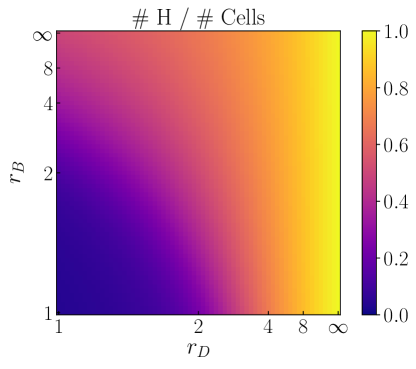
The most immediate quantity to calculate is the overall level of selection – that is, what is the final percentage of high affinity cells, number of H cells/?
Per timestep, let be the probability of a birth/division, and the probability of death. So,
To find the probability of a certain strain dividing, we let and use
where is just a normalization factor, and the individual probabilities are proportional to the strain’s population and birth fitness.
Similarly, to find the probability of a certain strain having a death, we use
where is a normalization factor, and the individual probabilities are proportional to the strain’s population and inversely proportional to its death fitness.
We will now use these probabilities to estimate the average change in H cells/ over time. First, the probability that the H population goes down by one is simply the probability that an H cell dies, so . To find the probability of a new H cell appearing, we need to consider three sources: an H cell divides (w/o mutation), an H cell divides (with an H H mutation), and an L cell divides (with an L H mutation). Putting these together, we get:
The average population of high affinity cells changes by every time step, so for large we can approximate by
| (1) |
We want to find the steady-state value of , so let’s assume we already hit , and therefore . So we want to solve
or equivalently,
For reasons which will be obvious later, let’s assume . Substituting in and rearranging, we get
Solving for (and taking the solution) gives
where
Therefore,
| (2) |
with the special case at being
| (3) |
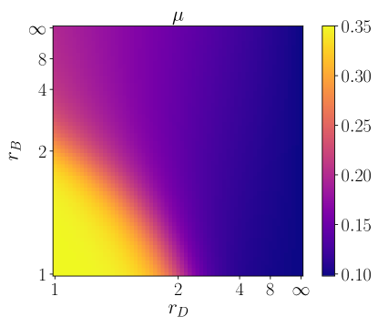
Notably, while is symmetric in and , the net level of selection is asymmetric in birth and death selectivity, as seen in figure 1. Consider the case where and , so high affinity cells are dividing at a much higher rate than low affinity cells. However, because the transition rate is nonzero, many of those new cells will be low affinity as well, and will stick around for a while because the negative selection pressure is nonexistent. In the limit of large , then
This means that there is an effective ceiling of selection for positive selection, wherein you will always have a mixture of high and low affinity, not matter how selective the system is. Meanwhile, with negative selection,
So negative selection has no ceiling whatsoever.
In particular, if a real-world evolutionary system is observed to have
then said system must have negative selection, since the force of positive selection alone is insufficient to attain that level of pressure.
Returning to the specific case of germinal centers, it is well established that a diversity of affinity levels persists. In experiments, even after three weeks, cells can be observed with a lower affinity than the initial seed population [34]. With this logic, if negative selection is present in germinal centers it should not be extremely strong, though this may also be an artifact of the gap between division and selection being long enough for us to observe cells slated for death.
IV The Ancestry Hypothesis
While this model may only two affinity levels, we can still have a diversity of genotypic strains via neutral mutations (e.g., high high affinity mutation). In principle, we can keep track of where these strains come from, therefore giving each strain an ancestor strain. We assume that the genotype space is large compared to the population of cells, so every new mutation produces a novel strain. That is to say, if strain A has a mutation during division, it will produce strain B, and if strain A has another mutation later on, that second mutation will be distinct from strain B.
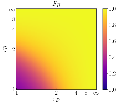
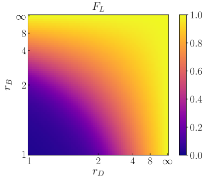
Looking at such phylogenetic trees, one might hypothesize that there may be a hidden signature of negative selection. One candidate signature is preferential ancestry. That is, we count how many high affinity cells have a high affinity strain as their ancestor, denoted by . Similarly, we let be the fraction of low affinity cells with a high affinity strain as an ancestor.
There are three distinct sources of high affinity cells. Per timestep, we attain an average of high affinity cells from nonmutating high affinity divisions, from mutating high affinity divisions, and from low to high affinity divisions. Similarly, there are two sources of H cells with H ancestors: on average we get such cells from non-mutating divisions, and from H cells mutating into other H cells.
Taking a steady-state, this means
Keeping in mind , then we have
| (4) |
By a similar accounting, we find that
| (5) |
Notably, both and only depend on positive and negative selection through their product . As seen by figures 2 and 3, these preferential ancestry ratios are perfectly symmetric in these two fitness parameters. Therefore, in this model, such metrics are ill suited for identifying the presence or absence of negative selection, since it makes no distinction between and .
Terminal Nodes
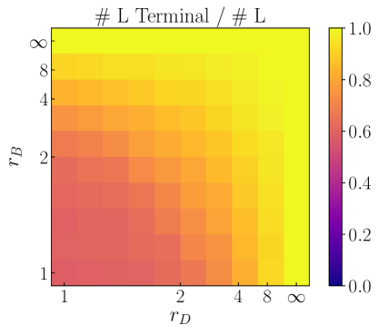
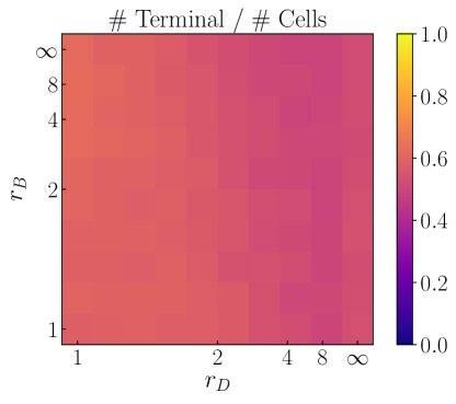
One related metric worth discussing here is the concept of “terminal nodes.” As the system of cells continues to divide and reproduce, strains will produce novel mutant descendants, creating a phylogenetic tree of ancestries. At any point of time, this tree will have terminal nodes, which are strains with no extant descendants. It can be conjectured that if most low affinity cells are in terminal nodes, then there ought to be negative selection at work.
A proper analytic exploration of this metric is somewhat out of scope of this paper, but we can generate examples numerically. In figure 4, we show the number of L cells in terminal nodes divided by the total number of L cells. Notice that this figure appears symmetric in and . Intuitively, this makes sense: if L cells only appear as terminal nodes, then either they die before they divide (high negative selection), or they don’t get a chance to divide in the first place (high positive selection).
Similarly, the total fraction of cells which are in terminal nodes shows poor signal in in figure 4. While it might be tempting to tease out a trend, it should be noted in real-world datasets, phylogenetic trees have to be attained via statistical reconstruction. The simulations here create the tree with perfect knowledge, whereas in practice there will be ambiguity over cell terminality, which would likely drown out whatever slight signal may be present.
In addition, most other ratios involving number of terminal cells can be derived from the prior two metrics, , , and the total selection level . While some terminal node metrics may have signals of negative selection, they would simply be from the signal present in the much easier to measure . Moreover, pilot simulations for counting number of genotypes (instead of number of cells) suggest the same results.
As such, it is hard to recommend any terminal node metric as a measure of negative selection.
V Mutation Count Distribution
Even though this model has only two phenotypes (low and high affinity), because of the large neutral space, the number of potential genotypes is extremely high. As before, we will assert that no two mutation events will ever be identical. That is, it is unlikely two separate mutation events will lead to the exact same base pair sequence. If we initialize the germinal center with a population of genetically identical cells, we should be able to count how many mutations are accumulated in each cell line.
If a species grows at a rate and has a mutation rate , then you’d expect the population to accrue mutations at an average rate of . In our model, we have two separate growth rates and mutation rates, & and & , but the actual average accumulation rate is somewhat more complicated due to the L H and H L mutations coupling the two mutation distributions.
More to the point, dynamically measuring a population’s mutational distribution is not always a good option. For many biological systems, doing a genotypic survey can be expensive and/or destructive (e.g., needing to destroy a germinal center to analyze its B cells), so measuring dynamical properties is usually unappealing.
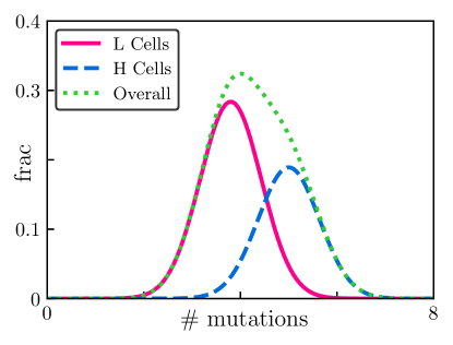
However, if the distribution of mutation counts is different between low and high affinity cells, then intuitively the overall mutation count distribution ought to be asymmetric. That is, we can hypothesize that the mutation count distribution ought to have some level of skew over long times, as in figure 6. Moreover, a back of the envelope calculations suggests that the skew would approach a constant value over time. Skew is calculated via the central moments , and a naive examination would suggest . Therefore, the skew would look like
Because this is a prediction of the long-term shape of the distribution, and not its dynamics, it can be measured and approximated by a single snapshot genotypic survey. The experimental advantage of taking one measurement over a longitudinal study need not be elaborated upon. Moreover, this final skew value should be a function of the different fitness parameters. Therefore, one can hypothesize that measuring mutational skew may be a good indicator of negative selection.
What follows is an explanation as to why this hypothesis is false.
To investigate the mutation count distribution, let’s assume that the overall affinity of the population has hit a steady state. Next, let us define to be the number of high affinity cells with mutations, divided by the total number of cells . Similarly, we let be the fraction of cells which are low affinity and have mutations, and . Note that , and .
To construct the dynamics for , we do some basic accounting. Sources for H cells with mutations are H and L cells with mutations, as well as H cells with mutations. In the single-mutant dynamics, the only sink is the natural death rate. Therefore, the dynamics are given by
To get the central moments , we first need the regular moments. To find the moments of the mutational distributions, we define the moments and for the H and L populations respectively. Taking of both sides, we get
| (6) | ||||
| (7) |
where we handled and by changing the sum index and using the binomial theorem, and taking .
While unpleasant to look at, this is fundamentally a linear system of equations. Moreover, since each ’th moment only depends on moments to , this gives it a block lower-triangular structure, which should be amenable to analysis. In principle, a closed-form solution involving matrix exponentials should be possible. However, in appendix C, we show that this approach is both numerically and theoretically fraught, due to the dynamical matrix becoming poorly conditioned over time. Therefore, a slightly different approach is needed.
To make analysis easier, we will instead use the following change of variables, and assume at least one of and are larger than 1:
| (8) | ||||
| (9) |
represents the ’th moment of the mutation count distribution for the overall population, including both H and L cells. Meanwhile, the definition of was just chosen to make the dynamics cleaner, as given by
| (10) | ||||
| (11) |
The prefactors are given by
and
is given by
Notice that always, so it functions as a proper timescale for the system.
Also note that only depends on lower order terms, meaning that it is possible to get exact solutions by iteratively solving. Both and will be polynomials in time with a maximum degree , plus some other terms that decay exponentially with rate .
Looking at the definitions of and in (8) and (9), it is easy to see and . By solving the differential equations for , we get
where the terms are just initial conditions, and . That is to say, the growth rate of the average number of mutations over time is , which can be rewritten as
| (12) |
Omitting the details of the recursion (which can be found in appendix D), we get that the leading order behavior for the ’th moment is given by
| (13) |
As expected, the ’th moment grows like , and the leading rate follows a simple form. The expression for the first correction (which is needed to calculate the distribution’s skew) is somewhat more unwelcoming, with
| (14) |
In order to calculate the mutation distribution’s skew and variance, we will need the central moments. The ’th central moment is defined by
Just as with the regular moments, these should be polynomials of maxium degree and decaying exponential corrections.
We don’t need the full solution for the central moment, just the leading growth term. But by some careful manipulation (also found in appendix D), we find that the supposed “leading” term is always zero,
| (15) |
When we try the next leading order term, we similarly find for that
| (16) |
However, for the special case of , we get
| (17) |
While has a term, we find has no term, has no term, and so on.
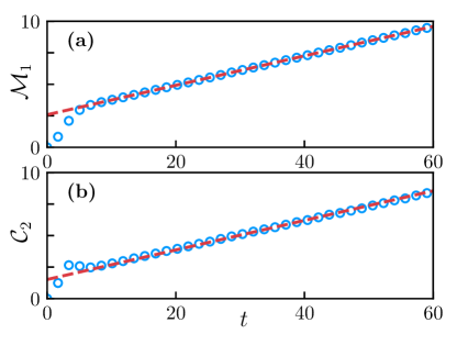
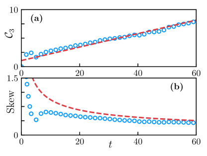
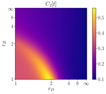
In particular, we now know that the variance (given by ) and the third central moment () must grow linearly in time. This is corroborated by simulation in figures 7a,7b, and 8a.
With this knowledge, we can finally estimate the skew of the mutant distribution. Plugging into the definition of skew, we find
| (18) |
This is supported by simulation results in 8b, where the skew indeed decays as . Therefore, there will be no long-term skew in the mutation count histogram, regardless of the choice of fitnesses. And so, the hypothesis outlined at the start of the section is false.
VI Discussion
Uncovering the mechanisms behind an evolutionary process is key – not only for advancing understanding and recreating natural systems [35, 36], but also for improving our own optimizing algorithms [2, 37, 38], and providing avenues for better medical interventions [22].
Based on our work, certain proposed metrics for measuring such mechanisms are ill suited for the task. Preferential ancestry ratios and mutational count asymmetry are particularly poor at the task, since in stable limits, all signature of mechanism vanishes.
The net selectivity, , is asymmetric in positive and negative fitness. However, it remains problematic for practical use. Outside of extreme cases, interpreting values of and out of a single would require detailed knowledge of mutation rates. However, since an evolutionary system may employ time-variable mutational adaptation (e.g., a cell line mutating rapidly while exposed to stress), rates measured in vitro may differ in vivo. Many other metrics we could propose here would have similar problems, or are simply redundant with . For example, if we were to take the average number of mutations in L cells and divide by the average among H cells, the ratio would converge to . While this is certainly asymmetric, it gives no new information compared to the more accessible metric .
This is not to say that no signature of mechanism exist – it is just that snapshot-style metrics have difficulty capturing dynamical differences. For example, the growth rate of average mutation count expresses mild asymmetry in figure 9, which only grows more pronounced when looking at the variance in figure 10. However, genotypic surveys, especially for microscopic cells, tend to be highly invasive, so the experimental burden of measuring any of these quantities may be too great to recommend.
However, perfect symmetry is rare in the real world. In an actual examination, one might expect that a quantity such as would have some asymmetry, or that the mutational skew would take on some long-term value, simply by the vagaries of nature. While the germinal center may have many black boxes, there are many in silica and in vitro experiments one can do which have highly controlled evolutionary mechanisms, some of which may contradict such perfect results. However, the model presented here is highly generic, especially considering the results from appendix A. If such a discrepancy were to be acknowledged, then it would cast doubt on many classes of mathematical evolutionary models.
One final complication specific to GCs may lie in the details of cyclic reentry. The essence of this scheme is that B cells move back and forth between two zones within the GC – a “dark zone” where division takes place, and a “light zone” where B cells are evaluated for affinity [24, 25, 39, 27, 12]. Many evolutionary models treat reproduction and fitness measurement as simultaneous. Here, there is ostensibly a period of “fitness blindness,” where cells live and divide unaware of their own affinity/fitness, introducing noise in the fitness landscape [40, 41]. Moreover, depending on how the mutation-proffering AID is used, the actual mutation rates of cell lines may wildly fluctuate, leading to hypothetical scenarios where the number of mutations is unproportional to the number of divisions. If that is the case, we may need to use a multistage, seasonal growth model [42].
Acknowledgements
This research was supported by the Center for Studies in Physics and Biology at Rockefeller University (B.O.-L.). We thank Arup Chakraborty, Kevin O’Keffee, Daniel Abrams, and Juhee Pae for the helpful comments.
Author Contributions
Bertrand Ottino-Loffler provided the main text, mathematical analysis, and numerics. Gabriel D. Victora provided the biological background and motivation.
References
- Darwin [1859] C. Darwin, On the origin of species (1859).
- Vrugt and Robinson [2007] J. A. Vrugt and B. A. Robinson, Improved evolutionary optimization from genetically adaptive multimethod search, Proceedings of the National Academy of Sciences 104, 708 (2007).
- Bäck and Schwefel [1993] T. Bäck and H.-P. Schwefel, An overview of evolutionary algorithms for parameter optimization, Evolutionary computation 1, 1 (1993).
- Bartz-Beielstein et al. [2014] T. Bartz-Beielstein, J. Branke, J. Mehnen, and O. Mersmann, Evolutionary algorithms, Wiley Interdisciplinary Reviews: Data Mining and Knowledge Discovery 4, 178 (2014).
- Yu and Gen [2010] X. Yu and M. Gen, Introduction to evolutionary algorithms (Springer Science & Business Media, 2010).
- Whitley et al. [1996] D. Whitley, S. Rana, J. Dzubera, and K. E. Mathias, Evaluating evolutionary algorithms, Artificial intelligence 85, 245 (1996).
- Tonegawa [1983] S. Tonegawa, Somatic generation of antibody diversity, Nature 302, 575 (1983).
- Eisen and Siskind [1964] H. N. Eisen and G. W. Siskind, Variations in affinities of antibodies during the immune response, Biochemistry 3, 996 (1964).
- Ada and Nossal [1987] G. L. Ada and S. G. Nossal, The clonal-selection theory, Scientific American 257, 62 (1987).
- McKean et al. [1984] D. McKean, K. Huppi, M. Bell, L. Staudt, W. Gerhard, and M. Weigert, Generation of antibody diversity in the immune response of balb/c mice to influenza virus hemagglutinin., Proceedings of the National Academy of Sciences 81, 3180 (1984).
- Note [1] There is also interest in the topic of broadly neutralizing antibodies [43, 44, 45], but here we will focus on narrow affinity maximization.
- Victora and Nussenzweig [2012] G. D. Victora and M. C. Nussenzweig, Germinal centers, Annual review of immunology 30, 429 (2012).
- Berek et al. [1991] C. Berek, A. Berger, and M. Apel, Maturation of the immune response in germinal centers, Cell 67, 1121 (1991).
- Amitai et al. [2017] A. Amitai, L. Mesin, G. D. Victora, M. Kardar, and A. K. Chakraborty, A population dynamics model for clonal diversity in a germinal center, Frontiers in microbiology 8, 1693 (2017).
- Gitlin et al. [2014] A. D. Gitlin, Z. Shulman, and M. C. Nussenzweig, Clonal selection in the germinal centre by regulated proliferation and hypermutation, Nature 509, 637 (2014).
- Liu et al. [1989] Y. Liu, D. Joshua, G. Williams, C. Smith, J. Gordon, and I. MacLennan, Mechanism of antigen-driven selection in germinal centres, Nature 342, 929 (1989).
- Meyer-Hermann [2021] M. Meyer-Hermann, A molecular theory of germinal center b cell selection and division, Cell Reports 36 (2021).
- Murray [1993] J. D. Murray, Mathematical biology (Springer, 1993).
- Kaveh et al. [2015] K. Kaveh, N. L. Komarova, and M. Kohandel, The duality of spatial death–birth and birth–death processes and limitations of the isothermal theorem, Royal Society open science 2, 140465 (2015).
- Yagoobi et al. [2023] S. Yagoobi, N. Sharma, and A. Traulsen, Categorizing update mechanisms for graph-structured metapopulations, Journal of the Royal Society Interface 20, 20220769 (2023).
- Ottino-Loffler et al. [2017] B. Ottino-Loffler, J. G. Scott, and S. H. Strogatz, Evolutionary dynamics of incubation periods, ELife 6, e30212 (2017).
- Young and Brink [2021] C. Young and R. Brink, The unique biology of germinal center b cells, Immunity 54, 1652 (2021).
- Tas et al. [2016] J. M. Tas, L. Mesin, G. Pasqual, S. Targ, J. T. Jacobsen, Y. M. Mano, C. S. Chen, J.-C. Weill, C.-A. Reynaud, E. P. Browne, et al., Visualizing antibody affinity maturation in germinal centers, Science 351, 1048 (2016).
- Oprea et al. [2000] M. Oprea, E. Van Nimwegen, and A. S. Perelson, Dynamics of one-pass germinal center models: implications for affinity maturation, Bulletin of mathematical biology 62, 121 (2000).
- Yaari et al. [2015] G. Yaari, J. I. Benichou, J. A. Vander Heiden, S. H. Kleinstein, and Y. Louzoun, The mutation patterns in b-cell immunoglobulin receptors reflect the influence of selection acting at multiple time-scales, Philosophical Transactions of the Royal Society B: Biological Sciences 370, 20140242 (2015).
- Victora et al. [2012] G. D. Victora, D. Dominguez-Sola, A. B. Holmes, S. Deroubaix, R. Dalla-Favera, and M. C. Nussenzweig, Identification of human germinal center light and dark zone cells and their relationship to human b-cell lymphomas, Blood, The Journal of the American Society of Hematology 120, 2240 (2012).
- Bannard et al. [2013] O. Bannard, R. M. Horton, C. D. Allen, J. An, T. Nagasawa, and J. G. Cyster, Germinal center centroblasts transition to a centrocyte phenotype according to a timed program and depend on the dark zone for effective selection, Immunity 39, 912 (2013).
- Oprea and Perelson [1997] M. Oprea and A. S. Perelson, Somatic mutation leads to efficient affinity maturation when centrocytes recycle back to centroblasts., Journal of immunology (Baltimore, Md.: 1950) 158, 5155 (1997).
- Allen et al. [1988] D. Allen, T. Simon, F. Sablitzky, K. Rajewsky, and A. Cumano, Antibody engineering for the analysis of affinity maturation of an anti-hapten response., The EMBO journal 7, 1995 (1988).
- Verhulst [1838] P.-F. Verhulst, Notice sur la loi que la population poursuit dans son accroissement, Correspondance Mathématique et Physique 10, 113 (1838).
- Cramer [2002] J. S. Cramer, The origins of logistic regression, Report (Tinbergen Institute, 2002).
- Petersen-Mahrt et al. [2002] S. K. Petersen-Mahrt, R. S. Harris, and M. S. Neuberger, Aid mutates e. coli suggesting a dna deamination mechanism for antibody diversification, Nature 418, 99 (2002).
- Muramatsu et al. [1999] M. Muramatsu, V. Sankaranand, S. Anant, M. Sugai, K. Kinoshita, N. O. Davidson, and T. Honjo, Specific expression of activation-induced cytidine deaminase (aid), a novel member of the rna-editing deaminase family in germinal center b cells, Journal of Biological Chemistry 274, 18470 (1999).
- Araki [2023] T. Araki, Replaying Life’s Tape With Intraclonal Germinal Center Evolution, Phd thesis, Rockefeller University (2023), available at https://digitalcommons.rockefeller.edu/student_theses_and_dissertations/720/.
- Sepkoski [2016] D. Sepkoski, “replaying life’s tape”: Simulations, metaphors, and historicity in stephen jay gould’s view of life, Studies in History and Philosophy of Science Part C: Studies in History and Philosophy of Biological and Biomedical Sciences 58, 73 (2016).
- Gould [1989] S. J. Gould, Wonderful life: the Burgess Shale and the nature of history (WW Norton & Company, 1989).
- Sharma and Traulsen [2022] N. Sharma and A. Traulsen, Suppressors of fixation can increase average fitness beyond amplifiers of selection, Proceedings of the National Academy of Sciences 119, e2205424119 (2022).
- Tkadlec et al. [2020] J. Tkadlec, A. Pavlogiannis, K. Chatterjee, and M. A. Nowak, Limits on amplifiers of natural selection under death-birth updating, PLoS computational biology 16, e1007494 (2020).
- Victora et al. [2010] G. D. Victora, T. A. Schwickert, D. R. Fooksman, A. O. Kamphorst, M. Meyer-Hermann, M. L. Dustin, and M. C. Nussenzweig, Germinal center dynamics revealed by multiphoton microscopy with a photoactivatable fluorescent reporter, Cell 143, 592 (2010).
- Trubenová et al. [2019] B. Trubenová, M. S. Krejca, P. K. Lehre, and T. Kötzing, Surfing on the seascape: Adaptation in a changing environment, Evolution 73, 1356 (2019).
- Merrell [1994] D. J. Merrell, The adaptive seascape: the mechanism of evolution (U of Minnesota Press, 1994).
- Swartz et al. [2022] D. W. Swartz, B. Ottino-Löffler, and M. Kardar, Seascape origin of richards growth, Physical Review E 105, 014417 (2022).
- Sok et al. [2013] D. Sok, U. Laserson, J. Laserson, Y. Liu, F. Vigneault, J.-P. Julien, B. Briney, A. Ramos, K. F. Saye, K. Le, et al., The effects of somatic hypermutation on neutralization and binding in the pgt121 family of broadly neutralizing hiv antibodies, PLoS pathogens 9, e1003754 (2013).
- Doria-Rose and Joyce [2015] N. A. Doria-Rose and M. G. Joyce, Strategies to guide the antibody affinity maturation process, Current opinion in virology 11, 137 (2015).
- Ferretti and Kardar [2023] F. Ferretti and M. Kardar, Universal characterization of epitope immunodominance from a multi-scale model of clonal competition in germinal centers, arXiv preprint arXiv:2310.10966 (2023).
Supplemental Information: On Possible Indicators of Negative Selection in Germinal Centers
Appendix A Asymmetric Mutation Rates
In this section, we will show that having non-identical mutation rates between the daughter cells produces the same results.
In particular, if an H cell divides, its first daughter has a chance of mutating into another H cell and a chance of becoming a L cell, and the second daughter has and . Similarly, the individual daughters of an L cell have an LL transition rate of and , and an LH transition rate of and respectively. We define the total transition rates as , , , and . To avoid trivial fixed points, we require and to be nonzero.
Note that while we require and to be nonzero, nothing prevents, say, . Here, one daughter would always be indistinguishable from the parent, which recreates the case from the main paper and some models of sexual reproduction. Similarly, if we want a more typical asexual reproduction model, setting the two daughters to have identical rates will do that for you.
Also, while instances of extreme mutation can be interesting, we shall also require and to be less than 1 to avoid some pathological regimes. For example, if , then would unintuitively cause the high fitness population to go extinct, since decreases per division.
On a division event, the total population of high fitness (H) cells can change by +2, +1, 0, -1, depending on the identity of the parent and the offspring. For example, if a low fitness (L) cell divides, and the first daughter mutates into a H cell and the second daughter is a nonmutated L cell, this would cause +1 new H cells. We notate this event as (), where the ’s identify the daughters as mutants, and the order tracks the identity of the daughters. Using this notation, we can write down all the H-changing events as
Given that is the fraction of the population which is H cells and is the fraction which is L cells, we can write the above events as probabilities to get
where and are defined as before. This simplifies into
This is identical to the equation in the single mutation case (section III in the main body), so all the results from that section would apply with the substitution and and the like. In particular,
If we are careful about accounting cells in the same manner as about, we retrieve familiar ancestry ratios and
We also get familiar equations for the number of mutations within strains, with
Hence, all results from the main body also apply to the general case of asymmetrically mutating daughters.
Appendix B Infinite fitness edge cases
Throughout this paper we considered only finite fitnesses, but on various heat plots, we include the case of and . Here we will discuss the approach for each. Moreover, for the sake of completeness, we will allow both daughters to be mutants, as in appendix A.
B.1 Limit of large positive selection.
In the case of infinite birth fitness, only high fitness cells divide. So and so long as . In such as case,
This means the average growth rate of high-fitness cells becomes
The steady state can be solved from here to get
Similarly, the equations for the mutant populations also get simplified, with
While simpler, the structure is similar to that in section V in the main body, so we can just take the results from there and take the limit of to quickly get the results. Notably, we have
As applied to the building blocks of equations for and (from section V in the main body), we have
Although some terms go to zero, this does not disrupt the rest of the analysis, leading to the same conclusion about the skew approaching zero.
B.2 Limit of large negative selection.
Although the limit of large positive selection was routine, a little more care must be taken with large negative selection. For example, trying to naively take the limit to the results of the main body’s section V leads to the timescale diverging.
Because of the high level of negative selection, so long as any L cells exist, no H cells will die. In fact, an attempt to write an equation for yields
Notably, this is strictly positive so long as . So, absent finite-size errors, is assured.
Because there is no low-fitness population worth talking about, we have that the H population is the full population, so . In particular, we have
where the term comes from the fact that at steady state, . We therefore have
This is recursively solvable, recalling that . Letting , the first three orders are given by
Therefore, the variance is given by
and the third central moment is given by
That is to say, the mean, variance, and third central moment all grow with at the exact same rate of . Therefore, the skew goes as
So, just as in the main case, we have no long-term skew appearing.
Appendix C The Matrix Exponential Solution
In the main body, we got equations for the moments of L and H populations
| (S1) | |||||||
| (S2) |
Let us vectorize the system in equations (S1) and (S2) by letting where we truncate to , since our goal is to find the skew. Therefore, the dynamics are given by
where the odd entries of are and the even entries are . Meanwhile, is a block matrix of the form:
with
and
So long as the determinant of is nonzero, this means that the moments are, in principle, exactly solvable, via
The determinant of is decided by . So calculating gives
If we calculate at population steady-state (), then we have
Therefore,
and so we get
As the system approaches a phenotypic equilibrium, we have . So if we want to find long-time dynamics (or worse, stationary state dynamics), then this vectorized formulation is ill suited for numerical and analytical examination.
Appendix D Recusion for Mutant Moments
In this section, we will produce the recursion equations that define the growth of the moments of the mutant distribution , and give the leading-order results for the central moments .
Specifically, we have the following system of equations
| (S3) | ||||
| (S4) |
where
| (S5) | ||||
| (S6) |
for all .
By hypothesis, we assume the solutions take the form of polynomials, with
| (S7) |
and
| (S8) |
where , , , and are coefficients to be determined, and we take coefficients with index to be zero.
Just as in the main text, the step is easy to verify. We start with the equation, and substitute appropriate values for and based on their definitions in (S5) and (S6), and get
For future notational convenience, we define
| (S9) |
Therefore, we have , where we use and .
Similarly, we have
Integrating gives us
so to leading order, the mean mutation count grows at a rate .
With a base established, we can create the inductive step to establish a recursion relation for the various coefficients. By subbing equations (S8) and (S7) into (S4), we get
where
| (S10) | ||||
| (S11) |
where we used lemma 3 in appendix E to collect terms appropriately, and we take the convention that when .
By a similar procedure, we have that
with
| (S15) | ||||
| (S16) |
If we plug these into the expressions in lemma 2 in appendix E, we then get
with
| (S17) | ||||
| (S18) | ||||
| (S19) |
If we insert (S16) and (S15) into equation (S17) and evaluate at , we get
| (S20) |
Similarly, if we insert (S11) and (S10) into equation (S12) and evaluate at , we find
| (S21) |
Putting equations (S20) and (S21) together gives the following closed forms via induction, using the fact that :
| (S22) | ||||
| (S23) |
If we instead evaluate (S12) and (S17) at , we get
Naturally, we can insert one into the other to find
If we then solve this via the lemma 4 in appendix E, we get for
Therefore, the subleading coefficient for the th moment is
| (S24) |
To recap, equation (S22) is the leading order coefficient of the growth of the th moment of mutation counts, and (S24) is the subleading coefficient. This gives us enough information to calculate the behavior of the central moments, which characterize the shape of the mutation count histogram.
The th central moment is given by
We take , since the first central moment is definitionally zero.
If we substitute in the polynomial forms of the terms and collect all the exponential terms under , we get
If we collect terms, this takes on the following form:
| (S25) | |||
where the bounds on the sum are from the first argument of needing to be less than , the second has to be less than , and their sum must be .
Via the general form of the moments (Equation (S8)), we know the leading term of the central moments grows at most as . So to get the proper coefficient, we evaluate the term to get
Note the use of equation (S22). Therefore, we have that for all , then
| (S26) |
In other words, every central moment grows at most as .
To find the order coefficient, we pull the term from Equation (S25). Here,
where we already inserted (S22). If we also insert (S24), we find
While this is unpleasant to look at, all the sums simplify to various Kronecker deltas . Keeping in mind and eliminating the appropriate deltas, this simplifies to
| (S27) |
This is nonzero when , and zero otherwise. This returns us to the results in the main text.
Appendix E Useful Lemmas
A number of elementary lemmas appear in our induction proofs, so for ease of reference they have been collected here.
Lemma 1.
Given the following equation for ,
we have the solution
with
Lemma 2.
Given the following equation for ,
we have the solution
with
Lemma 3.
Lemma 4.
If , then