A GLSM realization of derived equivalence
in $U(1)\times U(2)$ models

Abstract

The paper [1] has studied a derived equivalence between two Calabi-Yau fivefolds. In this paper, we propose a new understanding from the viewpoint of the GLSM, by realizing these two Calabi-Yau fivefolds in two different phases of a $U(1)\times U(2)$ GLSM. We find that this method can be generalized to construct other examples of derived equivalence. The functor for the equivalence can be realized by the brane transport along a path across different phases. To implement the brane transport, we compute the small window categories for anomalous $U(2)$ theories, extending previous results on window categories.

1 Introduction

The gauged linear sigma model (GLSM) with $\mathcal{N}=(2,2)$ supersymmetry has been a thriving research area that spawned many topics in both physics and mathematics. The boundary conditions of GLSMs that preserve a particular subset of the supersymmetries, known as B-branes, form a category, which is an important tool in analyzing the GLSMs. The objects of this category are matrix factorizations of the superpotential. The Kähler moduli space of a GLSM can be divided into several phases. If the low energy behaviour of a phase can be described by a nonlinear sigma model (NLSM) with target space $X$, then the B-brane category projects onto $D^{b}(X)$ the derived category of $X$ [2, 3, 4]. On the other hand, if the low energy behaviour of a phase is described by a Landau-Ginzburg (LG) model, then the low energy image of a GLSM brane in that phase is a matrix factorization of the LG model. Different phases have different sets of empty brane relations in general. Brane transport provides a functor between the B-brane categories of different phases of a GLSM [2, 5, 6]. In certain cases, this functor gives rise to an equivalence between the categories of B-branes. In particular, if two phases are described by two NLSMs with different target space $X_{+}$ and $X_{-}$ and the functor induced by the brane transport is an equivalence, then we get a derived equivalence between $X_{+}$ and $X_{-}$, i.e. $D^{b}(X_{+})\cong D^{b}(X_{-})$. Therefore GLSMs have been used to study a quite large class of manifolds and their derived equivalence (see for example [7, 8, 9, 10, 11, 12]).

There are certain constraints on brane transport. The situation depends on whether the Fayet-Iliopoulos (FI) parameter is renormalized under RG flow along the direction of the brane transport. In the Calabi-Yau (CY) case (also known as the non-anomalous case, meaning that the axial U(1) R-symmetry is anomaly free), in which the FI parameter is marginal, there are a number of sigular points on the Kähler moduli space (parameterized by the FI parameters) between the two phases, so the path along which the brane is transported must avoid these singularities. Given such a path, only the branes satisfying the grade restriction rule (GRR) can be smoothly transported from one phase to the other. The branes satisfying the grade restriction rule constitute a subcategory of the category of matrix factorizations of the GLSM, which is called the window category [2].

In the non-Calabi-Yau case (also known as the anomalous case, meaning that the axial $U(1)$ R-symmetry has anomaly), there are no singularities in the middle, but in order to determine the low energy image of a B-brane, one has to find an IR equivalent brane that is in the big window category, namely the category of branes satisfying the GRR. The low energy physics typically include a Higgs branch and some Coulomb/mixed branches, therefore the low energy limit of an anomalous GLSM matrix factorization has components on both Higgs and Coulomb/mixed branches. The small window category is a subcategory of the big window category, the objects in the small window category only have components on the Higgs branch in the low energy limit [6]. The grade restriction rules depend on the choice of the theta angle, and a shift of the theta-angle by certain amount results in a different but equivalent window category. In summary,

$$\begin{gathered}\text{{Matrix factorization}: GLSM B-branes}\\ \cup\\ \text{{Big window}: Branes that flow to both Higgs and mixed branches}\\ \cup\\ \text{{Small window}: Branes that only flow to Higgs branches}\end{gathered}$$

The GRR in both CY and non-CY cases have been studied and determined for abelian GLSMs [2, 5, 6]. However, the GRR for nonabelian GLSMs are not well understood. At this stage, there exists no general results and one has to resort to a case-by-case study. There are a few nonabelian examples where the GRR can be deduced (see, for example [5, 13]). In this paper, we advance this course by studying the GRR for nonabelian GLSMs with $U(2)$ gauge group and chiral fields in fundamental and determinantal representations. To get the result, we follow a categorical reasoning and an analysis of the hemisphere partition function.

In addition, with the GRR in hand, we study the derived equivalence between two manifolds, $X_{+}$ and $X_{-}$, by realizing them as the Higgs branches in different phases of a two-parameter nonabelian GLSM (the GLSM has two independent FI parameters) whose pure geometric phase realizes another manifold $\hat{X}$. In the examples we are going to consider, $\hat{X}$ will be either Fano or CY. Other than the pure geometric phase, there are also two other phases consisting of the Higgs branches $X_{\pm}$ and mixed branches $\mathcal{C}_{\pm}$. The derived equivalence between $X_{+}$ and $X_{-}$ is implemented by the brane transport along a path across the phases of this GLSM. This idea is sketched in Fig. 1. As a two-parameter model for the variety $\hat{X}$, it has two paths to transport the branes, one is from $\hat{X}$ to $(X_{+},\mathcal{C}_{+})$ and the other one is from $\hat{X}$ to $(X_{-},\mathcal{C}_{-})$. The fact we will use extensively in this paper is that the total Witten index in different phases are the same and this implies

$$\chi(\hat{X})\>=\>\chi(\hat{X}_{+})+\chi(\mathcal{C}_{+})\>=\>\chi(\hat{X}_{-})+\chi(\mathcal{C}_{-})\,.$$

With this picture in mind, we will show the derived equivalence between $X_{+}$ and $X_{-}$ via brane transport: for any object in $D^{b}(X_{+})$, we first lift it to a GLSM brane, use empty branes to grade restrict it if necessary, then transport it to the phase of $X_{-}$, where it can be projected to an object in $D^{b}(X_{-})$. One necessary condition for $X_{+}$ and $X_{-}$ to be derived equivalent is that their Euler characteristics should be equal to each other, namely, $\chi(X_{+})=\chi(X_{-})$. This condition implies nontrivial conditions on $X_{+}$ and $X_{-}$, and so on $\hat{X}$. This point will be more clear in section 4. However, sometimes it is difficult to compute their characteristics directly. For these cases, we instead compute the Witten indices of the mixed branches $\mathcal{C}_{\pm}$ which are easier to calculate. Matching of the Witten indices of $\mathcal{C}_{\pm}$ induces the same constraint due to the fact that the total Witten index is always the same.

$$\begindc{\commdiag}[300]\obj(1,3)[G]{GLSM}\obj(1,1)[xh]{\hat{X}}\obj(-1,0)[xp]{X_{+},\mathcal{C}_{+}}\obj(3,0)[xm]{X_{-},\mathcal{C}_{-}}\par\obj(-3,3)[uv]{UV}\obj(-3,1)[ir]{IR}\mor{uv}{ir}{}[\atright,\solidarrow]\par\mor{G}{xh}{\hat{\pi}}\mor{G}{xp}{\pi_{+}}\mor{G}{xm}{\pi_{-}}\par\mor{xp}{xh}{\mathbb{W}_{+}}[\atright,\dashArrow]\mor{xh}{xm}{\mathbb{W}_{-}}[\atright,\dashArrow]\enddc$$

Figure 1: Schematic diagram for the derived equivalence.

In order to implement the brane transport, we need to know the window categories of the local models at the phase boundaries [2, 12]. For the examples explored in this paper, the corresponding local models could be either abelian or non-abelian, and they could be non-anomalous or anomalous. Some of these local models are abelian gauge theories which have been previously studied [2, 6] and we will use their results directly. While the rest of the local models we will meet are $U(2)$ gauge theories with fundamental and determinantal representations. Although analysis of the window categories for such theories in the non-anomalous case exists [11], there are no known results in the anomalous cases. So before studying the B-branes in the $U(1)\times U(2)$ theories, we first analyze the window categories of the $U(2)$ theories in section 3.

Our original motivation of this work is to understand Segal’s proof of the derived equivalence between two non-compact Calabi-Yau fivefolds in [1] from a physics point of view. There, the two Calabi-Yau fivefolds, $X_{+}$ and $X_{-}$, are defined as the following:

$$X_{+}\>=\>\text{Tot}[(\wedge^{2}\mathcal{S})\otimes\mathcal{S}\to SGr(2,4)]\,,\quad X_{-}\>=\>\text{Tot}[(\mathcal{L}^{\perp}/\mathcal{L})\otimes\mathcal{L}^{2}\to\mathbb{P}^{3}]\,.$$

We will see this derived equivalence can be realized by an anomalous two-parameter GLSM with gauge group $U(1)\times U(2)$. The pure geometric phase has the target space

$$\hat{X}\>=\>{\rm Tot}[\mathcal{L}\otimes\wedge^{2}S\to SF(1,2,4)]\,,$$

where $SF(1,2,4)$ is the symplectic flag manifold. The full analysis for this example can be found in section 4.4. We also give a general construction and go beyond this example.

The organization of this paper is the following: in section 2, we will give a brief review of hemisphere partition functions and brane transport. Then, we generalize the idea to $U(2)$ gauge theories and derive the window categories in section 3. In section 4, we explicitly study several concrete examples, we start with an abelian gauge theory with gauge group $U(1)\times U(1)$ to illustrate the idea. Then we study the nonabelian theories with gauge group $U(1)\times U(2)$ including the theory corresponding to the derived equivalence between the Calabi-Yau fivefolds $X_{+}$ and $X_{-}$ mentioned above. At the end, we will give some concluding remarks and potential future directions in section 5. The appendix includes supplementary materials such as counting of Coulomb vacua and the analysis for the GLSM for a class of flag manifolds.

2 Review on hemisphere partition functions and window categories

In this section, we give a short review on the hemisphere partition functions of GLSMs. In particular, we review how we can extract big/small window categories from these hemisphere partitions, and this will be crucial for later sections. For more details, please refer to [2, 5, 6] and references therein.

2.1 Hemisphere partition functions

The data of a $\mathcal{N}=(2,2)$ GLSM model consists of gauge field content $\sigma_{a}$ valued in the Cartan subalgebra of the gauge group $G$, and the matter content:

$$\begin{array}[]{c|cc}&G&U(1)_{R}\\ \hline\cr X_{I}^{a}&Q_{I}^{a}&R_{I}\end{array}$$

for $I$ runs over all chiral fields and $a$ over weights under the Cartan subalgebra of $G$. The gauge charge for non-abelian $G$ is defined with respect to its Cartan subalgebra. $R_{I}$ is the charge under the $U(1)$ R-symmetry. A superpotential is a generic quasi-homogeneous polynomial $W(X)$ of matter fields, with its gauge charge $0$ and R-charge $2$. In the infrared, the classical Higgs branch, if exists, of this theory is the field configuration under gauging, known as geometric invariant theory quotient (GIT quotient). This geometry is represented as

$$X_{\xi}\>=\>\left\{\frac{\mathbb{C}^{I}-\Delta_{\xi}}{G}\right\}\cap\left\{\partial_{I}W(X)=0\right\}\,,$$ (1)

where $X_{\xi}$ depends on the Kähler cone of FI parameter $\xi$, and $\Delta_{\xi}$ is the discriminant locus in this phase. The dependence on $\xi$ is what is called the phase structure in [14].

One can assign different types of boundary conditions when the GLSM is put on a hemisphere [2, 5] and we are interested in the B-type boundary condition, which corresponds to a bound state coming from boundary terms of GLSM action of open string tachyon between Wilson line branes carrying gauge charges. The boundary condition is represented by a pair $\mathcal{B}=(Q,M)$ as a matrix factorization of the superpotential $W$ and a Lagrangian submanifold in the complexified Cartan subalgebra of the gauge group [15]. The pair $\mathcal{B}$ consists of an odd endomorphism $Q$ on a graded vector space $M$ such that

$$Q\circ Q=W\cdot\operatorname{Id}_{M}\,.$$ (2)

This matrix $Q$ has entries in polynomial ring of matter fields $X_{I}^{a}$, and it has gauge charge $0$ and R-charge $1$:

$$\begin{gathered}\rho_{G}(g)^{-1}\circ Q(g\circ X)\circ\rho_{G}(g)=Q(X)\,,\\ \rho_{R}(\lambda)\circ Q(\lambda\circ X)\circ\rho_{R}(\lambda)^{-1}=\lambda Q(X)\,,\end{gathered}$$

where $\rho_{R}$ and $\rho_{G}$ are the induced action on matrix factorization. It is useful to realize such $Q$ and $M$ in Clifford algebra and Clifford module. Given a factorization of polynomial $W$ as

$$W(X)\>=\>\sum_{i}g_{i}(X)\cdot f_{i}(X)\,,$$

if we introduce a pair of complex fermion operators $\psi_{i}$ and $\overline{\psi}_{i}$ satisfying the following anti-commutator relation:

$$\{\psi_{i},\overline{\psi}_{j}\}=\delta_{ij}\,.$$ (3)

Then, after assigning the proper R charge and gauge charges to fermion operators, one can write a matrix factorization as

$$Q=\sum_{i}g_{i}(X)\psi_{i}+f_{i}(X)\overline{\psi}_{i}$$ (4)

with graded module as the Hilbert space of free fermions

$$M=\bigoplus_{n}\bigoplus_{i_{1}<\cdots<i_{n}}\overline{\psi}_{i_{1}}\cdots\overline{\psi}_{i_{n}}|0\rangle\,,$$ (5)

where $\psi|0\rangle=0$. Using the anti-commutation relation (3), one can immediately see that

$$Q^{2}=\sum_{i}f_{i}(X)g_{i}(X)=W(X)\,.$$ (6)

The support of this brane as the zero locus of boundary fermion energy

$$\text{supp}(Q)=\big{\{}X\in\mathbb{C}^{I},\{Q(X),Q(X)^{\dagger}\}=0\big{\}}\,.$$ (7)

Gauge invariance of matrix factorization permits it to flow to the complex of coherent sheaves in the IR Higgs branch $X_{\xi}$, in which the support region $\mathrm{supp}(Q)$ determines the tachyon decay mode in different phases according to the discriminant locus $\Delta_{\xi}$.

The hemisphere partition function of a brane in $\mathcal{N}=(2,2)$ GLSM can be computed via the supersymmetric localization technique and was given in [5] as

$$Z_{\mathcal{B}}(t)\>=\>\int_{\gamma}d^{|G|}\sigma\prod_{\alpha\in\Delta^{+}_{G}}\alpha(\sigma)\sinh\pi\alpha(\sigma)\ \prod_{I}\Gamma\left(\sum_{a}iQ_{I}^{a}\sigma_{a}+\frac{R_{I}}{2}\right)e^{it(\sigma)}f_{\mathcal{B}}(\sigma)\,,$$ (8)

where $|G|$ denotes the dimension of Cartan subalgebra of $G$, $t(\sigma):=\langle t,\sigma\rangle$ is the pairing between the complexified FI-parameter $t=\xi-i\theta$ and the gauge field $\sigma$. Denote ${\hat{q}}_{a}$ and $\hat{R}$ as the charge operator for the induced action of $\rho_{G}$ and $\rho_{R}$ respectively, $f_{\mathcal{B}}(\sigma)$ is the brane factor evaluated on the gauge charge and R charges of graded module:

$$f_{\mathcal{B}}(\sigma)={\rm Tr}_{M}e^{i\pi\hat{R}}e^{2\pi\hat{q}_{a}\sigma_{a}}\,.$$ (9)

The integral in Eq. (8) is evaluated along a contour $\gamma$, which is a middle dimensional real class in the $\sigma$ space (a Lagrangian submanifold of the complexified Cartan subalgebra). In particular, this contour should be considered as a deformation from the real hyperplane in this space such that it avoids singularities of the gamma functions. Then the partition function can be computed as a sum of infinite many residues of gamma poles in a proper region depending on the phase determined by the FI-parameter $\xi$. After a specific choice of $\xi$, the poles are determined by the convergent region of the contour $\gamma$. In the large volume limit where $e^{-t}\rightarrow 0$, the leading term of $Z_{\mathcal{B}}$ evaluates the $\Gamma$-class of the bundle corresponding to $\mathcal{B}$, which is the data computed by boundary B-twisted theory, while the complete infinite summation comes from instanton effect computed by bulk A-twisted theory [5].

It is worth remarking that all methods above apply to the non-compact case $W=0$, where matrix factorization of zero is simply a differential. In this case, any R-charge of matter fields should be set to zero and separating poles in gamma-function may fail. However, a compact brane factor can be evaluated by regularizing gamma poles with small R-charge and taking the zero limit. A more systematic approach can be done by using the transformation law of residues in [16]. On the level of partition function, the existence of superpotential is known by R-charge assignment. Later, in section 4, we will see the example of Calabi-Yau 5-fold is a mixed case, i.e. it will have both a non-trivial superpotential and the non-compact direction.

2.2 Window and derived equivalence

In practice, there is a subtlety in choosing the contour $\gamma$ for $\mathcal{B}$, namely it may not have a convergent region for contour on a phase boundary for an arbitrary brane factor. Using Stirling’s formula, the partition function can be written asymptotically as

$$Z_{\mathcal{B}}(t)\sim\int d\sigma e^{F(\sigma,q,t)}$$ (10)

$$\sim\int_{\gamma}d^{|G|}\sigma\exp\bigg{\{}\sum_{I}iQ_{I}(\sigma)\log Q_{I}(\sigma)-\sum_{I}iQ_{I}(\sigma)+\pi\sum_{\Delta^{+}_{G}}|\alpha(\sigma)|+it(\sigma)-\sum_{M}2\pi q(\sigma)\bigg{\}}\,.$$

The absolutely convergent condition requires the negativity of the real part of the exponential in the integrand, which is

$$\mathrm{Re}[F(\sigma,q,t)]\>= \sum_{\Delta^{+}}\pi|\alpha(\tau)|+\big{(}-\xi_{R}(\nu)+(\theta+2\pi q)(\tau)\big{)}$$ (11)

$$+\sum_{I}Q_{I}(\nu)\big{[}\log|Q_{I}(\sigma)|-1\big{]}-|Q_{I}(\tau)|\left[\frac{\pi}{2}+\arctan\frac{Q_{I}(\nu)}{|Q_{I}(\tau)|}\right]\,,$$

with

$$\sigma=\tau+i\nu,\quad\operatorname{Arg}(iz)=\operatorname{sgn}(\mathrm{Re}[z])\left(\frac{\pi}{2}+\arctan\frac{\mathrm{Im}[z]}{\mathrm{Re}[z]}\right)\,,$$

for sufficiently large $|\sigma|$ on the contour when we move the parameter $t$ close to the radius of convergence. This condition picks out a specific range of admissible gauge charges in the brane. This range of gauge charges is called the window on a phase boundary. For example, a window of boundary $\xi=0$ in the $U(1)$ model of [2, section 7.3.1] is obtained by setting $\nu=0$ in the real exponential, $(\theta+2\pi q)\tau-\frac{\pi}{2}\sum_{I}|Q_{I}|\tau<0$, resulting in the grade restriction rule (GRR)

$$-\frac{\sum_{I}|Q_{I}|}{4}<q+\frac{\theta}{2\pi}<\frac{\sum_{I}|Q_{I}|}{4}\,.$$ (12)

One can see that the set of charges satisfying GRR depends on the choice of the $\theta$-angle, and this set is subject to an overall shift upon a $2\pi$-shift in the $\theta$ parameter. Different window categories defined by different $\theta$, whose objects are the branes with gauge charges satisfying the GRR, are categorically equivalent.

It was conjectured in [5] that branes with charges in the window correspond to the exceptional collection of the derived category of the geometry in the IR Higgs branch. The shift due to the $\theta$-angle corresponds to an automorphism of this collection by the Serre twist. The windows of non-abelian models are also systematically considered in [10, 11]. In the localization formula for the hemisphere partition function of the non-abelian models [5], the factors from positive roots of the gauge group will put non-trivial constraints on non-abelian charges. Depending on the matter content, it turns out that the window category of the GLSM for bundles over $Gr(k,n)$ can be either Kapranov’s, Kuznetsov’s or other exceptional collection.

In the non-anomalous case, the window only occurs on a phase boundary where parameters $e^{t}$ hit the radius of convergence. In the large volume limit, there should be no window constraints. The singularity on a phase boundary of $\xi$ is classical, however, this singularity can be lifted by quantum corrections due to the $\theta$-angle. Therefore, $Z_{\mathcal{B}}(t)$ can be analytically continued from one phase to another and this process is called brane transport. The derived equivalence of branes (sheaves) in different phases can be understood in this way.

In the case with superpotential, admissible branes are not only sheaves but also complexes of sheaves corresponding to matrix factorizations, which may not always lie in a window. As mentioned above, $\Delta_{\xi}$ corresponds to the semi-stable locus which is deleted in $X_{\xi}$, and this means a brane supported on this locus will be empty in this phase since it finds no where to take in $X_{\xi}$ as boundary condition. Then this bound state of branes is trivial as vacuum in $D^{b}(X_{\xi})$, or, equivalently, the corresponding complex is exact. Exactness of this bound state implies the annihilation from decayed open string tachyonic modes. This is known as the tachyon condensation of brane-anti-brane system. These trivial branes are called empty branes. By combining with empty branes, one can transform a brane complex exceeding the window to create a new but homologically equivalent brane complex, such that it is inside the window. This process is called grade restriction in [2].

In the IR limit, branes naturally decay via tachyon condensation. These IR branes can be lifted back to the UV Wilson line branes up to empty brane states. In conclusion, the derived equivalence in different phases of non-anomalous GLSMs are realized by brane transport, which is understood as an analytic continuation of hemisphere partition function of grade restricted brane across the phase boundaries. Such transport connects boundary conditions from one phase to another phase.

2.3 Big window v.s. small window

The discussion in the previous section only concerns the non-anomalous (Calabi-Yau) case. For the anomalous case, the situation is different. As mentioned in section 1, one has to distinguish between the big window and small window categories. In this case, the FI-parameters are subject to RG-flow. If the flow is from phase A to phase B, then in the IR we can only see phase B. But phase A can be reached by taking the gauge-decoupling limit, where the FI-parameter is fixed in the region corresponding to phase A at some fixed energy scale while the gauge coupling constant is taken to infinity [6]. Therefore, we can still use the techniques of brane transport to construct a functor between the categories of B-branes of phase A and phase B.

For any B-brane in phase A, we can lift it to a UV GLSM brane. Since there is an RG-flow on the space of FI-parameters, in order to read off the IR image of the GLSM brane, it has to be graded restricted so that the hemisphere partition function can be computed by a saddle point analysis. These grade restricted branes constitute the big window category. In general, phase B may consist of a Higgs branch and several Coulomb/mixed branches, so the IR brane will have components on Higgs and/or Coulomb/mixed branches. Only a subset of branes in the big window category has images only on the Higgs branch, which gives rise to the small window category. Therefore, the category of B-branes of the Higgs branch in the IR limit is equivalent to the small window category. Note that a $2\pi$-shift in $\theta$ angle will result in a different but equivalent big/small window category. In the Calabi-Yau case, the FI-parameters are marginal, and the big window and small window categories coincide.

As shown in [6], for any brane in the big window category, the contour integral can be computed by a saddle point analysis. The hemisphere partition function can then be written as a sum of residues corresponding to the Higgs branch and a contribution from the saddle points. The existence of the saddle points is an indication that the brane has components on the Coulomb/mixed branches in the IR limit. Therefore, for the image to be in the small window category, it should be possible to choose the contour such that there are no contribution to the hemisphere partition function from the saddle points. The saddle points are given by solutions to

$$\partial_{\sigma}F(\sigma,q,t)=0\,,$$ (13)

where $F$ is defined by the first line of Eq. (10). We will test this condition numerically and determine the possible region for small window. To do that, we plot the hypersurfaces determined by the saddle point equations on the contour, like in Fig.3, label the position of gauge charges admitting a solution, and then derive the maximal set of possible charges within them. By integrality we only need to test among the charges such that

$$q+\frac{\theta}{2\pi}\in\frac{1}{2}{\mathbb{Z}}\,.$$ (14)

We will demonstrate this analysis for $U(2)$ theories in the next section.

3 Small window of $U(2)$ theories

In this section, we will apply the above procedures in two concrete examples with $U(2)$ gauge group and obtain their small window categories. These two examples will later arise as the effective boundary theories (local model at the phase boundary [12]) in section 4, either on $\xi_{1}=0$ or on $\xi_{2}=0$. In principle, this method could be generalized to cases with higher rank gauge groups, but we leave this to future work.

3.1 One determinantal field

Let us first consider an $U(2)$ gauge theory with $n$ fundamental fields, $X_{i}$, $i=1,\dots,n$, and one field $P$ in the determinantal representation, $\det^{-m}$, with $m\leq n$, as summarized below

$$X_{i}$$

(15)

where $\xi$ is the associated FI parameter. This model has a vanishing superpotential, $W=0$. For later purpose, we will only focus on the cases with $n=3$ and $n=4$, and the same analysis in principle can be generalized to arbitrary $n$.

According to the D-term equations, the region $\xi\gg 0$ is a phase described by a total space of $m$-fold determinantal bundle over $Gr(2,n)$, i.e.

$$\mathrm{Tot}\left({\det}^{-m}\mathcal{S}\to Gr(2,n)\right)\,,$$

where $\mathcal{S}$ is the tautological bundle over the Grassmannian $Gr(2,n)$. Therefore, the total Witten index in this phase should be the Euler characteristic of this geometry, which is $\binom{n}{2}\,,$ This is also the number of generators of the big window category as we will see later.

Another region where $\xi\ll 0$ consists of a Higgs branch and some Coulomb vacua. The Coulomb branch behaviour at the large $\sigma$ region is determined by the one-loop corrected twisted superpotential and the Coulomb vacua equations are

$$\sigma_{a}^{n}\>=\>-q(-m)^{m}(\sigma_{1}+\sigma_{2})^{m},\quad a=1,2\,,$$

with excluded loci condition $\sigma_{1}\neq\pm\sigma_{2}$. One can count the number of Coulomb vacua and obtain

$$\left\lfloor\frac{n-1}{2}\right\rfloor(n-m)\,.$$ (16)

(The detailed computation is presented in appendix A.) The Higgs branch in this region is more complicated and, for our purpose, we need to extract the small window category which has pure Higgs branch contributions. And we will use the fact that the number of small window generators plus the number of Coulomb vacua equals the number of big window generators, as a consistency check.

To understand the Higgs branch of the phase with $\xi\ll 0$ and the small window category, let us do a category-theoretical analysis first, in the cases $n=3$ and $n=4$.

3.1.1 Higgs branch of the negative phase and its category of B-branes

When $m=n=3$, the negative phase can be understood via the IR duality of [17, 18]. The $U(2)$ theory (15) with $m=n=3$ is dual to the abelian GLSM, which has gauge group $U(1)$, three chirals with charge $1$ and one chiral with charge $-3$. The dual abelian GLSM has a phase corresponding to the limit $\xi\gg 0$ with target $\mathrm{Tot}(\mathcal{O}(-3)\rightarrow\mathbb{P}^{2})$, a noncompact Calabi-Yau manifold. The target space of the phase with $\xi\ll 0$ is the orbifold $\mathbb{C}^{3}/\mathbb{Z}_{3}$. The category of B-branes in this phase is the derived category $D^{b}(\mathbb{C}^{3}/\mathbb{Z}_{3})$, which is equivalent to the derived category of graded modules of $\mathcal{A}=\mathbb{C}[x_{1},x_{2},x_{3}]$, i.e. $D(\mathrm{gr}\text{-}\mathcal{A})$. This category is generated by $\mathcal{A}_{0},\mathcal{A}_{1},\mathcal{A}_{2}$, where $\mathcal{A}_{l}$ denotes the graded $\mathcal{A}$-module $\mathcal{A}$ with grading $l$ (the $\mathbb{Z}_{3}$-charge). $\mathcal{A}_{0},\mathcal{A}_{1},\mathcal{A}_{2}$ are mapped to $\pi^{*}\mathcal{O}_{\mathbb{P}^{3}},\pi^{*}\mathcal{O}_{\mathbb{P}^{3}}(1),\pi^{*}\mathcal{O}_{\mathbb{P}^{3}}(2)$ respectively via brane transport to the phase with $\xi\gg 0$, where $\pi$ is the projection onto the base $\mathbb{P}^{3}$. From the duality, we see the category of B-branes in the negative phase of the original $U(2)$ theory with $m=n=3$ is equivalent to $D(\mathrm{gr}\text{-}\mathcal{A})=\langle\mathcal{A}_{0},\mathcal{A}_{1},\mathcal{A}_{2}\rangle$. Because the orbifold group $\mathbb{Z}_{3}$ in this theory is a subgroup of $\det U(2)$, we see that $\mathcal{A}_{i}$ can be lifted to the GLSM brane $\mathcal{W}_{\det^{i+3l}}$. The window category is generated by $\mathcal{W}_{\det^{3l}},\mathcal{W}_{\det^{3l+1}},\mathcal{W}_{\det^{3l+2}}$ ($l$ depends on the choice of the theta-angle), which are mapped to $\det(\mathcal{S}^{\vee})^{3l},\det(\mathcal{S}^{\vee})^{3l+1},\det(\mathcal{S}^{\vee})^{3l+2}$ in the positive phase.

When $0<m<n=3$, there are $3-m$ Coulomb vacua in the negative phase and the category of B-branes of the Higgs branch, due to the $\mathbb{Z}_{m}$ orbifold, is generated by $m$ objects, namely $\mathcal{A}_{0},\cdots,\mathcal{A}_{m-1}$. Accordingly, the small window category is generated by $\mathcal{W}_{\det^{ml}},\mathcal{W}_{\det^{ml+1}},\cdots,\allowbreak\mathcal{W}_{\det^{ml+(m-1)}}$. The big window category remains the same as the window category of the $m=n=3$ theory.

The window category of the theory with $m=n=4$ is studied in [11]. The idea is as follows. The target space of the positive phase is the canonical line bundle $K_{Gr(2,4)}$. In the negative phase ($\xi\ll 0$), the $P$ field acquires a nonzero vev, which breaks $\det U(2)$ to a $\mathbb{Z}_{4}$ subgroup. Upon integrating out the fluctuation of $P$, we are left with a $SU(2)\times\mathbb{Z}_{4}$ gauge group, the $SU(2)$ fundamentals $X^{a}_{i}$ all have charge one under $\mathbb{Z}_{4}$. In the IR limit, the $SU(2)$ gauge group is decoupled, and the low energy degrees of freedom are described by the baryons

$$B_{ij}=\epsilon_{ab}X^{a}_{i}X^{b}_{j},\quad 1\leq i<j\leq 4\,,$$

which all have $\mathbb{Z}_{4}$ charge two.

Because $B_{ij}$ are the Plücker coordinates of the Grassmannian $Gr(2,4)$, the negative phase is expected to be a NLSM with target space

$$CGr(2,4)/\mathbb{Z}_{4}\,,$$

where $CGr(2,4)$ is the affine cone of the Plücker embedding of $Gr(2,4)$ in $\mathbb{P}^{5}$,

$$CGr(2,4)=\{(B_{12},B_{13},B_{14},B_{23},B_{24},B_{34})\in\mathbb{C}^{6}|f(B)=0\}\,,$$

where

$$f(B)=B_{12}B_{34}-B_{13}B_{24}+B_{14}B_{23}\,.$$

Indeed, there is a one-to-one correspondence between the generators of $D^{b}(K_{Gr(2,4)})$ and the generators of $D^{b}(CGr(2,4)/\mathbb{Z}_{4})$. Let $\mathcal{A}$ be the coordinate ring of $CGr(2,4)$, i.e.

$$\mathcal{A}\>=\>\mathbb{C}[B_{12},B_{13},B_{14},B_{23},B_{24},B_{34}]/\langle f(B)\rangle\,.$$

Then $D^{b}(CGr(2,4))\cong D(\mathrm{gr}\text{-}\mathcal{A})$, the derived category of graded $\mathcal{A}$-modules. Denote by $Perf(\mathcal{A})$ the subcategory of $D(\mathrm{gr}\text{-}\mathcal{A})$ whose objects are equivalent to finite-length complexes of free $\mathcal{A}$-modules of finite rank, and

$$D_{\mathrm{sg}}(\mathcal{A})\>=\>D(\mathrm{gr}\text{-}\mathcal{A})/Perf(\mathcal{A})\,.$$

We know $Perf(\mathcal{A})=\langle\mathcal{A}\rangle$, and (see [20, 21])

$$D_{\mathrm{sg}}(\mathcal{A})\>\cong\>\mathrm{MF}(f)\,,$$

where $\mathrm{MF}(f)$ is the category of matrix factorizations of $f$. Therefore there is a decomposition

$$D^{b}(CGr(2,4))\>=\>\langle\mathcal{A},\mathrm{MF}(f)\rangle\,.$$

Upon taking the $\mathbb{Z}_{4}$ orbifold action, we get

$$D(CGr(2,4)/\mathbb{Z}_{4})\>=\>\langle\mathcal{A}_{0},\mathcal{A}_{1},\mathcal{A}_{2},\mathcal{A}_{3},\mathrm{MF}_{\mathbb{Z}_{2}}(f)\rangle\,,$$ (17)

where $\mathcal{A}_{i}$ is the $\mathcal{A}$-module $\mathcal{A}$ with $\mathbb{Z}_{4}$ charge $i$. Notice that the $B_{ij}$’s all have $\mathbb{Z}_{4}$ charge 2 and $f$ is quadratic in $B_{ij}$, so we have $\mathrm{MF}_{\mathbb{Z}_{2}}(f)$ in Eq. (17) instead of $\mathrm{MF}_{\mathbb{Z}_{4}}(f)$.

The category $\mathrm{MF}_{\mathbb{Z}_{2}}(f)$ is the category of B-branes of the Higgs branch in the $\zeta\ll 0$ phase of the $U(1)$ GLSM with matter content

$$\begin{array}[]{c|ccccccc|c}&\Phi_{0}&\Phi_{1}&\Phi_{2}&\Phi_{3}&\Phi_{4}&\Phi_{5}&P&\\ \hline\cr U(1)&1&1&1&1&1&1&-2&\zeta\end{array}$$ (18)

and superpotential $W=Pf(\Phi)$. The phase with $\zeta\gg 0$ has pure Higgs branch whose target space is the quadric $\{f=0\}$ in $\mathbb{P}^{5}$, which is the image of $Gr(2,4)$ under the Plücker embedding. The category $\mathrm{MF}_{\mathbb{Z}_{2}}(f)$ is generated by the matrix factorization

and its $\mathbb{Z}_{2}$-twisted version (where the $\mathbb{Z}_{2}$ charges of the Chan-Paton spaces are flipped), where $\mathcal{M}=\mathbb{C}[\Phi_{0},\cdots,\Phi_{5}]^{\oplus 4}$ and the subscript indicates the $\mathbb{Z}_{2}$ charge. This fact can be seen from the fact that the small window category of the GLSM specified by (18) can only accommodate two consecutive $U(1)$ charges, and by counting the number of Coulomb vacua in the negative phase, it is clear that $\mathrm{MF}_{\mathbb{Z}_{2}}(f)$ is generated by two independent objects. These two matrix factorizations are mapped to the two spinor bundles[22] of the quadric via brane transport. The spinor bundles on $Gr(2,4)$ are the dual of the tautological bundle $\mathcal{S}^{\vee}$ and the universal quotient bundle $\mathcal{Q}$. Therefore, under the equivalence $D^{b}(CGr(2,4)/\mathbb{Z}_{4})\cong D^{b}(K_{Gr(2,4)})$, $\mathrm{MF}_{\mathbb{Z}_{2}}(f)$ is mapped to the subcategory of $D^{b}(K_{Gr(2,4)})$ generated by $\pi^{*}\mathcal{S}^{\vee}$ and $\pi^{*}\mathcal{Q}$, where $\pi$ is the projection $\pi:K_{Gr(2,4)}\rightarrow Gr(2,4)$.

In the $U(2)$ GLSM (15) with $n=m=4$ describing $K_{Gr(2,4)}$, because $\mathcal{A}_{i}$ has $\mathbb{Z}_{4}$ charge $i$, $\mathcal{A}_{i}$ can be lifted to a GLSM brane in the $\det^{i}$ representation, and it is mapped to $\pi^{*}(\det\mathcal{S}^{\vee})^{\otimes i}$ via brane transport.

Therefore, we have the following identification

$$\mathcal{A}_{i}\leftrightarrow\pi^{*}(\det\mathcal{S}^{\vee})^{\otimes i},\quad\mathrm{MF}_{\mathbb{Z}_{2}}(f)\leftrightarrow\langle\pi^{*}\mathcal{S}^{\vee},\pi^{*}\mathcal{Q}\rangle$$ (19)

for the equivalence

$$D^{b}(CGr(2,4)/\mathbb{Z}_{4})\>=\>\langle\mathcal{A}_{0},\mathcal{A}_{1},\mathcal{A}_{2},\mathcal{A}_{3},\mathrm{MF}_{\mathbb{Z}_{2}}(f)\rangle\cong D^{b}(K_{Gr(2,4)})\,.$$ (20)

Notice that

$$\mathcal{Q}\>\cong\>\det\mathcal{Q}\otimes\mathcal{Q}^{\vee}\>\cong\>\det\mathcal{S}^{\vee}\otimes(\mathcal{O}^{\oplus 4}\rightarrow\mathcal{S}^{\vee})\,,$$

the window category is generated by

$${\mathcal{W}}_{\cdot},{\mathcal{W}}_{\tiny{\yng(1)}},{\mathcal{W}}_{\tiny{\yng(1,1)}},{\mathcal{W}}_{\tiny{\yng(2,1)}},{\mathcal{W}}_{\tiny{\yng(2,2)}},{\mathcal{W}}_{\tiny{\yng(3,3)}}$$ (21)

up to a shift by $\mathcal{W}_{\det^{l}}$ induced by changing the theta-angle. The set of branes in (21) reduces to the semi-orthogonal decomposition

$$D^{b}(K_{Gr(2,4)})\>=\>\langle\mathcal{O},\mathcal{S}^{\vee},\det\mathcal{S}^{\vee},\det\mathcal{S}^{\vee}\otimes\mathcal{S}^{\vee},(\det\mathcal{S}^{\vee})^{\otimes 2},(\det\mathcal{S}^{\vee})^{\otimes 3}\rangle$$

in the positive phase. The equivalence (20) is an evidence that the IR theory of the negative phase is described by a NLSM with target space $CGr(2,4)/\mathbb{Z}_{4}$.

When $0<m<n=4$, the nonzero vev of $P$ breaks $\det U(2)$ to $\mathbb{Z}_{m}$, so we conjecture that the Higgs branch of the negative phase is described by a NLSM with target space $CGr(2,4)/\mathbb{Z}_{m}$. The subcategory $Perf(\mathcal{A})$ is thus generated by $m$ objects $\mathcal{A}_{0},\cdots,\mathcal{A}_{m-1}$. In addition, there are $4-m$ Coulomb vacua in this phases, therefore the singular subcategory $D_{\mathrm{sg}}(\mathcal{A})$ is still generated by ${4\choose 2}-m-(4-m)=2$ objects and we conjecture they are still mapped to $\pi^{*}\mathcal{S}^{\vee}$ and $\pi^{*}\mathcal{Q}$ in the positive phase. The small window category is thus expected to be generated by some $\det^{l_{1}}$ shift of $\langle\mathcal{W}_{\cdot},\mathcal{W}_{\tiny{\yng(1,1)}},\cdots,\mathcal{W}_{(m-1,m-1)}\rangle$ and some $\det^{l_{2}}$ shift of $\langle\mathcal{W}_{\tiny{\yng(1)}},\mathcal{W}_{\tiny{\yng(2,1)}}\rangle$, where $l_{1}-l_{2}$ can be determined by analyzing the hemisphere partition function, and the overall shift is determined by the theta-angle.

3.1.2 Hemisphere partition function and the window categories

Now let us obtain the big and small windows from the hemisphere partition functions, as discussed in section 2. For general $m\leq n$, the real exponential factor is given by ($\sigma_{a}=\tau_{a}+i\nu_{a}$, $t=\xi-i\theta$)

$$A_{q}(t)\>= \pi|\tau_{1}-\tau_{2}|-\xi(\nu_{1}+\nu_{2})+\theta(\tau_{1}+\nu_{1})+2\pi(q_{1}\tau_{1}+q_{2}\tau_{2})$$ (22)

$$+m(-\nu_{1}-\nu_{2})\left(\log|m(\sigma_{1}+\sigma_{2})|-1\right)-m|\tau_{1}+\tau_{2}|\left(\frac{\pi}{2}-\arctan\frac{\nu_{1}+\nu_{2}}{|\tau_{1}+\tau_{2}|}\right)$$

$$+n\left[\nu_{1}\left(\log|\sigma_{1}|-1\right)-|\tau_{1}|\left(\frac{\pi}{2}+\arctan\frac{\nu_{1}}{|\tau_{1}|}\right)\right]$$

$$+n\left[\nu_{2}\left(\log|\sigma_{2}|-1\right)-|\tau_{2}|\left(\frac{\pi}{2}+\arctan\frac{\nu_{2}}{|\tau_{2}|}\right)\right]\,.$$

If we take the contour [11]

$$\gamma\>=\>\left\{\nu_{1}\>=\>-\nu_{2}\>=\>\tau_{1}^{2}-\tau_{2}^{2}\right\}\,,$$ (23)

then the following wedge conditions [5, 11]

$$\tau_{1}\>=\>0\quad\Rightarrow \quad\nu_{1}\>\leq\>0\,;$$ (24)

$$\tau_{2}\>=\>0\quad\Rightarrow \quad\nu_{2}\>\leq\>0\,;$$ (25)

$$\tau_{1}+\tau_{2}\>=\>0\quad\Rightarrow \quad\nu_{1}+\nu_{2}\>\geq\>0$$ (26)

are satisfied so the contour will not hit the singularities. Along the contour (23), we have

$$A_{q}(t)\>= \pi|\tau_{1}-\tau_{2}|+\left(\theta+2\pi q_{1}\right)\tau_{1}+\left(\theta+2\pi q_{2}\right)\tau_{2}-\pi\frac{m}{2}|\tau_{1}+\tau_{2}|-\pi\frac{n}{2}(|\tau_{1}|+|\tau_{2}|)$$ (27)

$$-n|\tau_{1}|\arctan\left(\frac{(\tau_{1})^{2}-(\tau_{2})^{2}}{|\tau_{1}|}\right)-n|\tau_{2}|\arctan\left(\frac{(\tau_{1})^{2}-(\tau_{2})^{2}}{|\tau_{2}|}\right)$$

$$+((\tau_{1})^{2}-(\tau_{2})^{2})\frac{n}{2}\log\frac{(\tau_{1})^{2}+((\tau_{1})^{2}-(\tau_{2})^{2})^{2}}{(\tau_{2})^{2}+((\tau_{1})^{2}-(\tau_{2})^{2})^{2}}\,.$$

Then the convergence condition is given by [11, 12]

$$\begin{gathered}\left|\frac{\theta}{2\pi}+q_{1}+\frac{\theta}{2\pi}+q_{2}\right|\>\leq\>\frac{n+m}{2}\,,\\ \left|\frac{\theta}{2\pi}+q_{\alpha}\right|\>\leq\>\frac{2n-2+m}{4}\,,\\ \left|q_{1}-q_{2}\right|\>\leq\>\frac{n-2}{2}\,.\end{gathered}$$ (28)

However, this condition is not restrict enough and it gives more charges in the window than expected. Fortunately, there are certain relationships from the Eagon-Northcott complex associated to a matrix, among the branes in the relaxed window [23], so the number of independent generators in the window will be exactly the Euler characteristic of $Gr(2,n)$. For $m=n$, the convergent region is shown in Fig. 2, in which the axis are parameterized by $q_{a}+\theta/{2\pi}$, where $q_{1}$ and $q_{2}$ are the charges under the Cartan of $U(2)$.

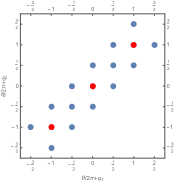
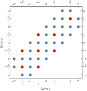
Figure 2: Admissible charges in $\frac{1}{2}\mathbb{Z}$ and an integral choice of $\mathbb{W}_{\mathrm{Big}}$ in red for $n=3$ (left) and $n=4$ (right).

The admissible charges are marked as blue dots in Fig. 2, among which the big window category consists of charges marked red, which correspond to representations

$$\mathbb{W}_{\mathrm{Big}}\>=\>\left\{\begin{array}[]{cl}\left\langle\cdot,\ \tiny{\yng(1)},\ \tiny{\yng(1,1)}\right\rangle\,,&n=3\,,\\ \\ \left\langle\cdot,\ \tiny{\yng(1)},\ \tiny{\yng(1,1)},\ \tiny{\yng(2)},\ \tiny{\yng(2,2)},\ \tiny{\yng(3,3)}\right\rangle\,,&n=4\,.\end{array}\right.$$ (29)

They correspond to the semi-orthogonal decomposition of the derived category of ${\mathbb{P}}^{2}(\cong Gr(2,3))$ and $Gr(2,4)$ respectively. Note that in the case of $n=4$, half of the off-diagonal charges is equivalent to the other half by binding with the empty branes [11].

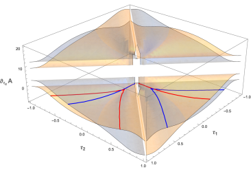
Figure 3: Numerical illustration of $\partial_{\tau_{a}}A_{q}(\tau_{1},\tau_{2})$ and zero contours. The light yellow sheet is the plot for $\partial_{\tau_{1}}A_{q}(\tau_{1},\tau_{2})$ while the red contour indicates the solutions to $\partial_{\tau_{1}}A_{q}(\tau_{1},\tau_{2})=0$. The light blue sheet and the blue contour are for $\partial_{\tau_{2}}A_{q}(\tau_{1},\tau_{2})$ and its zero loci.

Next, in order to obtain the small window, one should rule out the solutions to the saddle point equations

$$\partial_{\tau_{\alpha}}A_{q}(\tau_{1},\tau_{2})\>=\>0,\quad\alpha=1,2\,,$$ (30)

among the admissible charges on the contour $\gamma$, (23). More explicitly, $\partial_{\tau_{\alpha}}A_{q}$ restricted on $\gamma$ are given as

$$\partial_{\tau_{1}}A_{q}|_{\gamma}\>= \left(2\pi q_{1}+\theta\right)+n\tau_{1}\log\left(\frac{(\tau_{1})^{2}+((\tau_{1})^{2}-(\tau_{2})^{2})^{2}}{(\tau_{2})^{2}+((\tau_{1})^{2}-(\tau_{2})^{2})^{2}}\right)-n\tan^{-1}\left(\frac{(\tau_{1})^{2}-(\tau_{2})^{2}}{\tau_{1}}\right)$$ (31)

$$-2n\frac{\tau_{1}(\tau_{1}-\tau_{2})(\tau_{1}+\tau_{2})(((\tau_{1})^{2}-(\tau_{2})^{2})^{2}-(\tau_{2})^{2})}{((\tau_{1})^{4}+(\tau_{2})^{4}+(\tau_{1})^{2}(1-2(\tau_{2})^{2}))((\tau_{2})^{2}+((\tau_{1})^{2}-(\tau_{2})^{2})^{2})}$$

$$-\frac{\pi}{2}\left(n\operatorname{sign}(\tau_{1})+m\operatorname{sign}(\tau_{1}+\tau_{2})-2\operatorname{sign}(\tau_{1}-\tau_{2})\right)\,,$$

and

$$\partial_{\tau_{2}}A_{q}|_{\gamma}\>= \left(2\pi q_{2}+\theta\right)+n\tau_{2}\log\left(\frac{(\tau_{2})^{2}+((\tau_{1})^{2}-(\tau_{2})^{2})^{2}}{(\tau_{1})^{2}+((\tau_{1})^{2}-(\tau_{2})^{2})^{2}}\right)-n\tan^{-1}\left(\frac{(\tau_{1})^{2}-(\tau_{2})^{2}}{\tau_{2}}\right)$$ (32)

$$-2n\frac{\tau_{2}(\tau_{2}-\tau_{1})(\tau_{1}+\tau_{2})(((\tau_{2})^{2}-(\tau_{1})^{2})^{2}-(\tau_{1})^{2})}{((\tau_{1})^{4}+(\tau_{2})^{4}+(\tau_{1})^{2}(1-2(\tau_{2})^{2}))((\tau_{2})^{2}+((\tau_{1})^{2}-(\tau_{2})^{2})^{2})}$$

$$-\frac{\pi}{2}\left(n\operatorname{sign}(\tau_{2})+m\operatorname{sign}(\tau_{1}+\tau_{2})+2\operatorname{sign}(\tau_{1}-\tau_{2})\right)\,.$$

To see when Eq. (30) has no solution, we apply a numerical method. For example, for $n=3,m=1$ with $q_{\alpha}+\theta/2\pi=(-1/2,-1/2)$, $\partial_{\tau_{1}}A_{q}(\tau_{1},\tau_{2})=0$ and $\partial_{\tau_{2}}A_{q}(\tau_{1},\tau_{2})=0$ are plotted as the red and blue contours in Fig. 3. Then, the transversal intersection between the red and blue contours implies the solutions to the Coulomb vacuum equations, and therefore the corresponding representation should be ruled out from the small window.

The numerical results are summarized as in Fig. 4, where the gray background indicates convergent region, black points are the charges such that Eq. (30) has saddle point solutions, which should be ruled out, and the red points correspond to the charges in the small window.

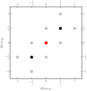
(a) n=3,m=1

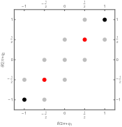
(b) n=3,m=2

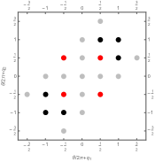
(c) n=4,m=1

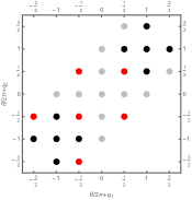
(d) n=4,m=2

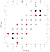
(e) n=4,m=3

Figure 4: Saddle point solutions (black) and the admissible integer charges in small window (red).

According to the numerical results, one can conclude that small windows of this non-abelian GLSM are given as the following:

• $n=3$

  $${\begin{array}[]{ll}m=1,&\mathbb{W}_{\mathrm{Small}}\>=\>\left\langle\cdot\right\rangle\\ m=2,&\mathbb{W}_{\mathrm{Small}}\>=\>\left\langle\cdot,\quad{\tiny\yng(1,1)}\right\rangle\\ m=3,&\mathbb{W}_{\mathrm{Small}}\>=\>\left\langle\cdot,\quad{\tiny\yng(1,1)},\quad{\tiny\yng(2,2)}\right\rangle\end{array}}$$ (33)

• $n=4$

  $${\begin{array}[]{ll}m=1,&\mathbb{W}_{\mathrm{Small}}\>=\>\left\langle\cdot,\quad\tiny\yng(1),\quad\tiny\yng(1,1)\right\rangle\\ m=2,&\mathbb{W}_{\mathrm{Small}}\>=\>\left\langle\tiny\yng(1),\quad\tiny\yng(1,1),\quad\tiny\yng(2,1),\quad\tiny\yng(2,2)\right\rangle\\ m=3,&\mathbb{W}_{\mathrm{Small}}\>=\>\left\langle\tiny\yng(1),\quad\tiny\yng(1,1),\quad\tiny\yng(2,1),\quad\tiny\yng(2,2),\quad\tiny\yng(3,3)\right\rangle\\ m=4,&\mathbb{W}_{\mathrm{Small}}=\left\langle\cdot,\quad\tiny\yng(1),\quad\tiny\yng(1,1),\quad\tiny\yng(2,1),\quad\tiny\yng(2,2),\quad\tiny\yng(3,3)\right\rangle\end{array}}$$ (34)

If one counts the number of generators in the small windows, one can conclude that, in the cases of $n=3$ and $n=4$,

$$\chi_{-}\>=\>\text{the number of generators of~{}}\mathbb{W}_{\mathrm{Small}}\>=\>\left\{\begin{array}[]{ll}m\,,&n=3\,,\\ m+2\,,&n=4\,,\end{array}\right.$$

and together with the number of Coulomb vacua (16), one can see that they match the total Witten index and the above analysis is consistent:

$$\chi_{+}\>=\>\text{the number of generators of~{}}\mathbb{W}_{\mathrm{Big}}\>=\>\chi_{-}+\left\lfloor\frac{n-1}{2}\right\rfloor(n-m)\>=\>\binom{n}{2}\,.$$ (35)

3.2 Two determinantal fields

Let us consider a slightly generalized model with one more determinantal fields, namely it is defined by the following GLSM data

$$X_{i}$$

and the superpotential is again zero, $W=0$. One can see that this GLSM realizes a similar pure Higgs branch in the positive FI region,

$$\mathrm{Tot}\left[{\det}^{m_{1}}(\mathcal{S})\oplus{\det}^{m_{2}}(\mathcal{S})\rightarrow Gr(2,n)\right]\,,$$ (36)

which has the same Witten index as $Gr(2,n)$. On the other hand, the negative FI region consists of a Higgs branch and some Coulomb vacua. The Coulomb vacua are determined by the equations

$$\sigma_{a}^{n}=-q(-m_{1})^{m_{1}}(-m_{2})^{m_{2}}(\sigma_{1}+\sigma_{2})^{m_{1}+m_{2}},\quad a=1,2\,.$$

Again, one can count the number of Coulomb vacua as in appendix A,

$$N(n,m_{1},m_{2})\>=\>\left\lfloor\frac{n-1}{2}\right\rfloor(n-m_{1}-m_{2})\,.$$

On the Higgs branch of the negative phase, the nonzero vev of $P_{1}$ and $P_{2}$ furnishes the weighted projective space $W\mathbb{P}(m_{1},m_{2})$. The baryons $B_{ij}=\varepsilon_{\alpha\beta}X^{\alpha}_{i}X^{\beta}_{j}$ are coordinates along the fiber of the vector bundle $\mathcal{O}^{\oplus{n\choose 2}}(-1)$ over the weighted projective space. But there are relationships between the baryon fields, so the target space in the negative phase is a fiber bundle over $W\mathbb{P}(m_{1},m_{2})$ with each fiber being isomorphic to the affine cone of $Gr(2,n)$.

In the case $n=3$, the affine cone of $Gr(2,3)$ is just $\mathbb{C}^{3}$, therefore the target space is just $Y=\mathrm{Tot}(\mathcal{O}^{\oplus 3}(-1)\rightarrow W\mathbb{P}(m_{1},m_{2}))$, and $D^{b}(Y)$ is generated by $\mathcal{O}(i)$, $i=0,1,\cdots,m_{1}+m_{2}-1$. So the number of generators of $D^{b}(Y)$ plus the number of Coulomb vacua is 3, which is exactly the Euler characteristic of $Gr(2,3)$ as expected.

In the case $n=4$, the target space $Y$ is a fiber bundle over $W\mathbb{P}(m_{1},m_{2})$ with each fiber being the quadric in $\mathbb{C}^{6}$ corresponding to the affine cone of the Grassmannian $Gr(2,4)$. Even though the orbifold groups in the coordinate patches of $W\mathbb{P}(m_{1},m_{2})$ are generally different from each other, the number of generators corresponding to the spinor bundles should be independent of the orbifold structure as argued in section 3.1.1, and thus independent of $m_{1}$ and $m_{2}$. So the spinor bundles constitute two generators of $D^{b}(Y)$. In addition, there are $m_{1}+m_{2}$ generators given by $\mathcal{O}(i)$, $i=0,1,\cdots,m_{1}+m_{2}-1$. Again, the the number of generators of $D^{b}(Y)$, which is $m_{1}+m_{2}+2$, plus the number of Coulomb vacua, which is $4-m_{1}-m_{2}$, is 6, which is equal to the Euler characteristic of $Gr(2,4)$.

One can analyze the hemisphere partition function as before to find out the small and big windows, and in this case the exponential factor is similarly given by:

$$A_{q}(t)\>= \pi(\tau_{1}-\tau_{2})-\xi(\nu_{1}+\nu_{2})+\theta(\tau_{1}+\nu_{1})+2\pi(q_{1}\tau_{1}+q_{2}\tau_{2})$$ (37)

$$+(m_{1}+m_{2})(-\nu_{1}-\nu_{2})\left(\log|m_{1}(\sigma_{1}+\sigma_{2})|-1\right)$$

$$-(m_{1}+m_{2})|\tau_{1}+\tau_{2}|\left(\frac{\pi}{2}-\arctan\frac{\nu_{1}+\nu_{2}}{|\tau_{1}+\tau_{2}|}\right)$$

$$+n\left[\nu_{1}\left(\log|\sigma_{1}|-1\right)-|\tau_{1}|\left(\frac{\pi}{2}+\arctan\frac{\nu_{1}}{|\tau_{1}|}\right)\right]$$

$$+n\left[\nu_{2}\left(\log|\sigma_{2}|-1\right)-|\tau_{2}|\left(\frac{\pi}{2}+\arctan\frac{\nu_{2}}{|\tau_{2}|}\right)\right]\,,$$

and on the contour $\gamma$, it is reduced to

$$A_{q}(t)\>= \pi|\tau_{1}-\tau_{2}|+\left(\theta+2\pi q_{1}\right)\tau_{1}+\left(\theta+2\pi q_{2}\right)\tau_{2}-\pi\frac{m_{1}+m_{2}}{2}|\tau_{1}+\tau_{2}|-\pi\frac{n}{2}(|\tau_{1}|+|\tau_{2}|)$$ (38)

$$-n|\tau_{1}|\arctan\left(\frac{(\tau_{1})^{2}-(\tau_{2})^{2}}{|\tau_{1}|}\right)-n|\tau_{2}|\arctan\left(\frac{(\tau_{1})^{2}-(\tau_{2})^{2}}{|\tau_{2}|}\right)$$

$$+((\tau_{1})^{2}-(\tau_{2})^{2})\frac{n}{2}\log\frac{(\tau_{1})^{2}+((\tau_{1})^{2}-(\tau_{2})^{2})^{2}}{(\tau_{2})^{2}+((\tau_{1})^{2}-(\tau_{2})^{2})^{2}}\,,$$

which is the same as (27) when $m=m_{1}+m_{2}$. Therefore, the previous discussions and computations can be directly applied here by changing $m$ to $m_{1}+m_{2}$. So, the small and big windows are given by that of $m=m_{1}+m_{2}$ in the examples given in the last subsection. For the cases we are interested in, $n=3$ and $n=4$, the consistency relation still holds as in Eq. (35).

4 Examples

In this section, we will implement the method broadcast in the introduction and use results from the previous section to study the derived equivalence in concrete examples. As a warmup, we first start with an abelian example in section 4.1, which highlights many of the features of this analysis. In sections 4.2, 4.3 and 4.4, we then study three nonabelian examples and analyze the corresponding derived equivalences.

Remarks on the notation.

For all the examples considered in this section, we will always use $\hat{X}$ to denote the target space of the geometric phase of the GLSM, while $X_{\pm}$ as the target space of the Higgs branch, accompanied by a mixed branch $\mathcal{C}_{\pm}$, in a different phase of the same GLSM.

4.1 Orbibundle over projective space

As the first example, we will consider the derived equivalence between two orbibundles, $X_{+}$ and $X_{-}$, which are defined as the following

$$X_{+}\>=\>[{\rm Tot}(\mathcal{O}(-n/m)^{\oplus M}\to\mathbb{P}^{N-1})/(\mathbb{Z}_{m^{\prime}}\times\mathbb{Z}_{g})]\,,$$ (39)

$$X_{-}\>=\>[{\rm Tot}(\mathcal{O}(-m/n)^{\oplus N}\to\mathbb{P}^{M-1})/(\mathbb{Z}_{n^{\prime}}\times\mathbb{Z}_{g})]\,,$$

where $g=\gcd(m,n)$, $n^{\prime}=n/g$, $m^{\prime}=m/g$. $X_{+}$ and $X_{-}$ can be realized in two different phases of a GLSM with $\hat{X}$ as its target space in the pure geometric phase, where

$$\hat{X}\>=\>{\rm Tot}(\mathcal{O}(-m,-n)\to\mathbb{P}^{M-1}\times\mathbb{P}^{N-1})\,.$$ (40)

In order to ensure the derived equivalence between $X_{+}$ and $X_{-}$, the constraint $mN=nM$ must hold, which is also the Calabi-Yau condition for both $X_{+}$ and $X_{-}$.

4.1.1 GLSM construction

To realize $\hat{X}$ , we consider the GLSM with $U(1)\times U(1)$ gauge group and it is defined by the following matter content for the chiral fields

$$\Phi_{a}$$

with $a=1,\dots,M$ and $i=1,\dots,N$. $\xi_{1}$ and $\xi_{2}$ are the FI parameters. We assume $m<M,n<N$ so the axial $U(1)$ R-symmetry has anomaly. There is no superpotential in this model and the classical vacua are determined by the $D$-term equations, which are

$$\sum_{a=1}^{M}|\Phi_{a}|^{2}-m|P|^{2}\>=\>\xi_{1}\,,\quad\sum_{i=1}^{N}|X_{i}|^{2}-n|P|^{2}\>=\>\xi_{2}\,.$$ (41)

The effective twisted superpotential on the Coulomb branch is given as

$$\widetilde{W}_{\rm eff}(\sigma_{1},\sigma_{2})\>= -t_{1}\sigma_{1}-t_{2}\sigma_{2}-M\sigma_{1}\left(\log\sigma_{1}-1\right)-N\sigma_{2}\left(\log\sigma_{2}-1\right)$$

$$-(-m\sigma_{1}-n\sigma_{2})\left(\log(-m\sigma_{1}-n\sigma_{2})-1\right)\,$$

and therefore the Coulomb branch equations are

$$\sigma_{1}^{M} \>=\>q_{1}(-m\sigma_{1}-n\sigma_{2})^{m}\,,$$ (42)

$$\sigma_{2}^{N} \>=\>q_{2}(-m\sigma_{1}-n\sigma_{2})^{n}\,,$$

with $q_{a}=\exp(-t_{a})$ and the $t_{a}$’s are the FI-$\theta$ parameters.

4.1.2 Phases

As depicted in Fig. 5, this GLSM has three different phases: $\{\xi_{1}\gg 0,\xi_{2}\gg 0\}$, $\{\xi_{1}\ll 0,n\xi_{1}\ll m\xi_{2}\}$ and $\{\xi_{2}\ll 0,n\xi_{1}\gg m\xi_{2}\}$. Let us go through these phases and analyze their IR behaviour.

Figure 5: Phases for the abelian two-parameter model.

Phase I: $\xi_{1}\gg 0$ and $\xi_{2}\gg 0$.

This phase is a pure geometric phase, and the target space is

$$\hat{X}\>=\>{\rm Tot}(\mathcal{O}(-m,-n)\to\mathbb{P}^{M-1}\times\mathbb{P}^{N-1})\,,$$

which can be read off from the D-term equations (41). One can also confirm this by analysing the asymptotic behaviour of the Coulomb branch equations (42) in the deep phase limit, $\xi_{1}\to+\infty$ and $\xi_{2}\to+\infty$. In this limit, the only solution to the Coulomb vacuum equations is $\sigma_{1}=\sigma_{2}=0$, which indicates that this phase only has a pure Higgs branch.

Then the Witten index in this phase only has contributions from the Euler characteristic of the target space $\hat{X}$, which is $MN$.

Phase II: $\xi_{1}\ll 0$ and $n\xi_{1}\ll m\xi_{2}$.

This phase consists of a Higgs branch and some mixed Higgs-Coulomb branches. One can see this by looking at the behaviour of solutions to the Coulomb branch equations (42) in the limit $\xi_{1}\to-\infty$ and $\xi_{2}\to+\infty$ such that $n\xi_{1}<m\xi_{2}$. In this limit, $\sigma_{2}\to 0$ and then the first equation becomes

$$\sigma_{1}^{M}=q_{1}(-m)^{m}\sigma_{1}^{m}\,,$$

which has total $M$ solutions and $m$ of them are zero solutions while the other $(M-m)$ solutions are non-zero. Namely, now we have $m$ zero solutions $(\sigma_{1},\sigma_{2})=(0,0)$ and $(M-m)$ solutions with $(\sigma_{1},\sigma_{2})=(\ast,0)$ where $\ast$ is one of the solutions to equation $\sigma_{1}^{M-m}=q_{1}(-m)^{m}$.

The solution $(\sigma_{1},\sigma_{2})=(0,0)$ suggests that there exists a pure Higgs branch, which can be read from the D-term equations. To describe the Higgs branch, one can change the basis for the Lie algebra of the gauge group and obtain

$$\Phi_{a}$$ P

0

where $g=\mathrm{gcd}(m,n)$, and $\mu$ and $\nu$ are a pair of integers such that $\mu m^{\prime}+\nu n^{\prime}=1$. Since $\xi_{1}\ll 0$, the $P$ field should take the non-vanishing expectation value $\left<P\right>=\sqrt{-\xi_{1}/m}$. As such, the gauge group breaks to a subgroup $U(1)_{s}\times\mathbb{Z}_{g}$, where $U(1)_{s}:=n^{\prime}U(1)_{1}-m^{\prime}U(1)_{2}$ and its associated FI parameter is $\xi_{s}:=n^{\prime}\xi_{1}-m^{\prime}\xi_{2}$. Once the fluctuation of the $P$ field is integrated out, the remaining massless degrees of freedom are

$$\Phi_{a}$$

(43)

and because $\xi_{s}\ll 0$, one can immediately find out that the pure Higgs branch has target space

$$X_{+}\>=\>[{\rm Tot}(\mathcal{O}(-n^{\prime}/m^{\prime})^{\oplus M}\to\mathbb{P}^{N-1})/({\mathbb{Z}}_{m^{\prime}}\times{\mathbb{Z}}_{g})]\,,$$

where the orbifold group acts trivally on the base space, and its action on the fiber can be read from (43). The Euler characteristic of $X_{+}$ can be computed as

$$\chi(X_{+})\>=\>|{\mathbb{Z}}_{m^{\prime}}\times{\mathbb{Z}}_{g}|\cdot\chi(\mathbb{P}^{N-1})\>=\>mN\,.$$

At the nonzero solutions $(\sigma_{1},\sigma_{2})=(\ast,0)$, the fields $\Phi_{a}$ and $P$ will be massive and should be integrated out. What left is an effective GLSM for $\mathbb{P}^{N-1}$ defined by $U(1)_{2}$ with $N$ chiral fields $X_{i}$ of charge $1$. In summary, the whole structure of this phase can be described as in Fig. 6.

Figure 6: Mixed structure of Phase II.

Now, let us count the Witten index as a consistency check. There are two types of contributions: one is from the pure Higgs branch $X_{+}$ and the other one is from the $(M-m)$ mixed Higgs-Coulomb branches ($M-m$ copies of $\mathbb{P}^{N-1}$). Therefore, the total Witten index is the sum of these two contributions

$$mN+(M-m)N=MN\,,$$

matching the result in Phase I.

Phase III: $\xi_{2}\ll 0$ and $n\xi_{1}\gg m\xi_{2}$.

This phase has a similar mixed structure as Phase II, including: one Higgs branch, which is $X_{-}=[{\rm Tot}(\mathcal{O}(-m^{\prime}/n^{\prime})^{\oplus N}\to\mathbb{P}^{M-1})/{\mathbb{Z}}_{n^{\prime}}\times{\mathbb{Z}}_{g}]$, and $(N-n)$ mixed Higgs-Coulomb branches, namely $\mathbb{P}^{M-1}$ located at $(N-n)$ non-zero points on the $\sigma_{2}$-plane. We skipped the details here, but one can also check the matching of the total Witten index

$$nM+(N-n)M=MN.$$

4.1.3 Effective theories on the phase boundaries

Now we want to implement the brane transport along the path illustrated in Fig. 5 to find a functor realizing the equivalence between $D^{b}(X_{+})$ and $D^{b}(X_{-})$. Apparently, this requires the understanding of the effective local models at the phase boundaries, $\{\xi_{1}=0,\xi_{2}\gg 0\}$ and $\{\xi_{1}\gg 0,\xi_{2}=0\}$, and the small window categories thereof.

The local model at the phase boundary $\{\xi_{1}=0,\xi_{2}\gg 0\}$ has the following matter content

$$\Phi_{a}$$

(44)

Therefore, the small window category consists of the branes with $U(1)_{1}$ charges $q_{1}$ satisfying

$$\left|q_{1}+\frac{\theta_{1}}{2\pi}\right|<\frac{m}{2},$$

which is termed band restriction rule in [2]. Thus, with a suitable choice of the $\theta$-angle, the small window category at the phase boundary $\{\xi_{1}=0,\xi_{2}\gg 0\}$ is generated by branes of the form $\mathcal{W}(i,q)$, where $0\leq i\leq m-1,q\in{\mathbb{Z}}$.

The local model at the phase boundary $\{\xi_{1}\gg 0,\xi_{2}=0\}$ has the following matter content

$$X_{i}$$

(45)

Therefore, the small window category consists of the branes with $U(1)_{2}$ charges $q_{2}$ satisfying the band restriction rule

$$\left|q_{2}+\frac{\theta_{2}}{2\pi}\right|<\frac{n}{2}.$$

Thus, with a suitable choice of the theta-angle, the small window category at the phase boundary $\{\xi_{1}\gg 0,\xi_{2}=0\}$ is generated by branes of the form $\mathcal{W}(q,j)$, where $-n+1\leq j\leq 0,q\in{\mathbb{Z}}$.

4.1.4 Brane transport and derived equivalence

We are interested in studying the derived equivalence between $X_{+}$ and $X_{-}$. One necessary condition is that their Euler characteristics coincide, namely $mN=nM$. As discussed before, we have realized them in different phases of the GLSM for $\hat{X}={\rm Tot}(\mathcal{O}(-m,-n)\to\mathbb{P}^{M-1}\times\mathbb{P}^{N-1})$. In the GLSM construction, $X_{\pm}$ are accompanied with the mixed Higgs-Coulomb branches $\mathcal{C}_{\pm}$ respectively. In this example,

$$\mathcal{C}_{+}\>=\>\left\{(M-m)\text{ copies of }\mathbb{P}^{N-1}\ \text{located at $(M-m)$ nonzero points on $\sigma_{1}$-plane}\right\}\,,$$

$$\mathcal{C}_{-}\>=\>\left\{(N-n)\text{ copies of }\mathbb{P}^{M-1}\ \text{located at $(N-n)$ nonzero points on $\sigma_{2}$-plane}\right\}\,.$$

The Witten index contributions from $\mathcal{C}_{\pm}$ should also match, i.e. $(M-m)N=(N-n)M$, which is exactly the same as $mN=nM$ as one would expect. One also immediately recognize that the condition, $mN=nM$, is also the Calabi-Yau condition for both $X_{+}$ and $X_{-}$.

The deleted sets on the phases are given by

$$X_{+}: \ \{X=0\}\cup\{P=0\}$$ (46)

$$\hat{X}: \ \{X=0\}\cup\{\Phi=0\}$$

$$X_{-}: \ \{\Phi=0\}\cup\{P=0\}$$

and the corresponding Koszul complexes of empty branes on these deleted sets are

$$\begin{gathered}\mathcal{E}_{X}:\quad\mathcal{W}(q,-N)\xrightarrow{X}\mathcal{W}(q,-N+1)^{\oplus N}\xrightarrow{X}\cdots\xrightarrow{X}\mathcal{W}(q,-1)^{\oplus N}\xrightarrow{X}\mathcal{W}(q,0),\\ \mathcal{E}_{\Phi}:\quad\mathcal{W}(-M,q)\xrightarrow{\Phi}\mathcal{W}(-M+1,q)^{\oplus M}\xrightarrow{\Phi}\cdots\xrightarrow{\Phi}\mathcal{W}(-1,q)^{\oplus M}\xrightarrow{\Phi}\mathcal{W}(0,q),\\ \mathcal{E}_{P}:\quad\mathcal{W}(m,n)\xrightarrow{P}\mathcal{W}(0,0),\end{gathered}$$ (47)

from which $\mathcal{E}_{P}$ will be used to grade restrict UV brane complexes into the small windows. As we assume $m<M,n<N$, the FI parameters are subject to renormalization. If the FI parameters $(\xi_{1},\xi_{2})$ are above the line $n\xi_{1}=m\xi_{2}$, then they will end up in the phase of $X_{+}$ in the IR limit under RG flow. The RG flow will take a UV GLSM brane $\mathcal{W}(p_{1},p_{2})$ to an IR brane on $X_{+}$ as

$$\mathcal{W}(p_{1},p_{2})\xrightarrow{\pi_{+}}\mathcal{O}_{X_{+}}\left(\frac{p_{2}m^{\prime}-p_{1}n^{\prime}}{m^{\prime}}\right)_{s},$$ (48)

where $s\equiv\mu p_{1}+\nu p_{2}~{}(\mathrm{mod}~{}g)$ labels the twisted sector of $\mathbb{Z}_{g}$. On the other hand, if the FI parameters $(\xi_{1},\xi_{2})$ are below the line $n\xi_{1}=m\xi_{2}$, then they will end up in the phase of $X_{-}$ in the IR limit. A UV GLSM brane $\mathcal{W}(p_{1},p_{2})$ will descend to an IR brane on $X_{-}$ as

$$\mathcal{W}(p_{1},p_{2})\xrightarrow{\pi_{-}}\mathcal{O}_{X_{-}}\left(\frac{p_{1}n^{\prime}-p_{2}m^{\prime}}{n^{\prime}}\right)_{s}.$$ (49)

Notice that if we use $\mathcal{E}_{P}$ to replace $\mathcal{W}(p_{1},p_{2})$ with an IR equivalent brane $\mathcal{W}(p_{1}-lm,p_{2}-ln)$ for some integer $l$, then both $i=q_{2}m^{\prime}-q_{1}n^{\prime}$ and $s\equiv\mu(p_{1}-lm)+\nu(p_{2}-ln)\equiv\mu p_{1}+\nu p_{2}~{}(\mathrm{mod}~{}g)$ are invariant, therefore the IR images under $\pi_{+}$ and $\pi_{-}$ are indeed unchanged.

Consequently, the brane transport between $D^{b}(X_{+})$ and $D^{b}(X_{-})$ is given by the following procedure:

• For any $i\in\{0,1,\cdots,m^{\prime}N-1\},s\in{\mathbb{Z}}_{g}$, choose a pair of integers $(p_{1},p_{2})$ such that $i=p_{2}m^{\prime}-p_{1}n^{\prime}$ and $s\equiv\mu p_{1}+\nu p_{2}~{}(\mathrm{mod}~{}g)$. For example,

  $$p_{1}=-\nu i+m^{\prime}s+lm,\ p_{2}=\mu i+n^{\prime}s+ln,\ \forall~{}l\in\mathbb{Z}.$$

• Then, from Eq. (48), The lift of a brane $\mathcal{O}_{X_{+}}\left(\frac{i}{m^{\prime}}\right)_{s}$ in the phase of $X_{+}$ (above the line $n\xi_{1}=m\xi_{2}$) is

  $$\mathcal{O}_{X_{+}}\left(\frac{i}{m^{\prime}}\right)_{s}\xrightarrow{\pi_{+}^{-1}}\mathcal{W}(p_{1},p_{2}),$$ (50)

• Use the IR empty brane $\mathcal{E}_{P}$ to grade restrict $\mathcal{W}(p_{1},p_{2})$ so the resulting brane is in the small window category at the phase boundary $\{\xi_{1}=0,\xi_{2}\gg 0\}$, i.e. $p_{1}=0,\cdots,m-1$, so it can pass through this phase boundary.

• Once in the phase $\{\xi_{1}\gg 0,\xi_{2}\gg 0\}$, we can move it below the line $n\xi_{1}=m\xi_{2}$ and use the IR empty brane $\mathcal{E}_{P}$ to grade restrict it such that it is in the small window category at the phase boundary $\{\xi_{1}\gg 0,\xi_{2}=0\}$, i.e. $p_{2}\in\{-n+1,-n+2,\cdots,1,0\}$. Then the brane can be transported to the phase of $X_{-}$.

• Due to Eq. (49), the brane can be projected to give the image:

  $$\mathcal{W}(\overline{p}_{1},\overline{p}_{2})\xrightarrow{\pi_{-}}\mathcal{O}_{X_{-}}\left(-\frac{i}{n^{\prime}}\right)_{s},$$

  where $\overline{p}_{1}$ and $\overline{p}_{2}$ are the resulting gauge charges after the grade restriction has been applied.

In conclusion, with our choice of the small windows, the brane transport yields the following map between the generators of $D^{b}(X_{+})$ and $D^{b}(X_{-})$:

$$\mathcal{O}_{X_{+}}\left(\frac{i}{m^{\prime}}\right)_{s}\Rightarrow\mathcal{O}_{X_{-}}\left(-\frac{i}{n^{\prime}}\right)_{s}$$

for $i=0,1,\cdots,m^{\prime}N-1,~{}s\in{\mathbb{Z}}_{g}$.

Example:

$m=4,n=6$, $M=6$, $N=9$.
In this case, $g=\gcd(m,n)=2,m^{\prime}=2,n^{\prime}=3$ and we can take $\mu=-1,\nu=1$. The geometries are

$$\begin{gathered}X_{+}=[\mathrm{Tot}(\mathcal{O}(-3/2)^{\oplus 6}\rightarrow\mathbb{P}^{8})/(\mathbb{Z}_{2}\times\mathbb{Z}_{2})]\,,\\ X_{-}=[\mathrm{Tot}(\mathcal{O}(-2/3)^{\oplus 9}\rightarrow\mathbb{P}^{5})/(\mathbb{Z}_{3}\times\mathbb{Z}_{2})]\,.\end{gathered}$$

The small window at the phase boundary $\{\xi_{1}=0,\xi_{2}\gg 0\}$ is generated by $\mathcal{W}(i,p_{2})$, where $i=0,1,2,3$ and $p_{2}$ is any $U(1)_{2}$ charge. The small window at the phase boundary $\{\xi_{1}\gg 0,\xi_{2}=0\}$ is generated by $\mathcal{W}(p_{1},j)$, where $j=-5,-4,\cdots,0$ and $p_{1}$ is any $U(1)_{1}$ charge.

The derived category $D^{b}(X_{+})$ is generated by ${\mathcal{O}}_{X_{+}}\left(\frac{i}{2}\right)_{s}$ with $i=0,1,\cdots,17,~{}s=0,1$. The derived category $D^{b}(X_{-})$ is generated by ${\mathcal{O}}_{X_{-}}\left(-\frac{j}{3}\right)_{t}$ with $j=0,1,\cdots,17,~{}t=0,1$. For any $i$ and $s$ in the range indicated above, take

$$p_{1}=-i+2s,\quad p_{2}=-i+3s.$$

The lift of ${\mathcal{O}}_{X_{+}}\left(\frac{i}{2}\right)_{s}$ is $\mathcal{W}(p_{1}+4l,p_{2}+6l)$ for any integer $l$. We can first choose $l$ such that $p_{1}+4l\in\{0,1,2,3\}$. After the brane is transported to the phase $\{\xi_{1}\gg 0,\xi_{2}\gg 0\}$, we can choose another integer $l^{\prime}$ such that $p_{2}+6l+6l^{\prime}\in\{-5,-4,\cdots,0\}$ so the grade restricted brane can be transported to the phase of $X_{-}$, where its IR image is ${\mathcal{O}}_{X_{-}}\left(-\frac{i}{3}\right)_{s}$.

4.2 Product of a projective space and a Grassmannian

In the previous section, we have presented our strategy for showing the derived equivalence in an abelian gauge theory. Now, in this section, we start to consider a nonabelian example and show the derived equivalence between $X_{+}$, a vector bundle over Grassmannian as defined by Eq. (56), and $X_{-}$, a fibre bundle over projective space as defined by Eq. (58). We follow a similar construction as discussed in the previous section and find that $X_{+}$ and $X_{-}$ can be realized in two different phases of the GLSM for $\hat{X}$, which is a fiber bundle over the product of a projective space and a Grassmannian, Eq. (53).

4.2.1 GLSM construction

The GLSM has the gauge group $U(1)\times U(2)$ and the following matter content

$$X_{a}$$

1 0

(51)

with $\alpha=1,2$ the $U(2)$ color index, $a=1,\cdots,M$ and $j=1,\dots,N$ are flavor indices, and we assume $m\leq M,n\leq N$. In this model, the superpotential $W=0$. The Coulomb vacuum equations are

$$\sigma^{M} =q_{1}(-m\sigma-n\sigma_{1}-n\sigma_{2})^{m}\,,$$ (52)

$$\sigma_{\alpha}^{N} =-q_{2}(-m\sigma-n\sigma_{1}-n\sigma_{2})^{n}\,,\alpha=1,2\,,$$

where $\sigma$ is the scalar component of the gauge field strength associated with $U(1)$, while $\sigma_{\alpha},\alpha=1,2$ are those associated with the Cartan subalgebra of $U(2)$. In the above, $q_{s}:=\exp(-t_{s})$ and $t_{s}$ is the FI-$\theta$ parameter corresponding to $\xi_{s}$.

4.2.2 Phases

The phase diagram for this GLSM is the same as the previous example, i.e. Fig. 5. Clearly, in the $\xi_{1}\gg 0,\xi_{2}\gg 0$ region, there is only a pure Higgs branch with target space

$$\hat{X}\>=\>\mathrm{Tot}\left(\mathcal{O}_{\mathbb{P}^{M-1}}(-m)\otimes\left(\det\mathcal{S}\right)^{\otimes n}\rightarrow\mathbb{P}^{M-1}\times Gr(2,N)\right)\,,$$ (53)

where $\mathcal{S}$ is the tautological bundle over $Gr(2,N)$. The total Witten index in this phase equals the Euler characteristic of $\hat{X}$, which is

$$\chi(\hat{X})\>=\>M\binom{N}{2}\,.$$ (54)

If either $\xi_{1}\ll 0$ or $\xi_{2}\ll 0$, the $P$ field gets a nonzero vev due to the D-term equations and breaks the $U(1)\times\det U(2)$ gauge group to a subgroup $U(1)_{s}\times{\mathbb{Z}}_{\gcd(m,n)}$ with the FI parameter of $U(1)_{s}$ given by $\xi_{s}:=n^{\prime}\xi_{1}-m^{\prime}\xi_{2}$, where $m^{\prime}=m/{\gcd(m,n)},n^{\prime}=n/{\gcd(m,n)}$. Under the $U(1)_{s}$ gauge group, the $SU(2)$ invariant fields $X_{a}$ and the baryon fields $B_{ij}=\varepsilon_{\alpha\beta}\Phi^{\alpha}_{i}\Phi^{\beta}_{j}$ have charges

$$X_{a}$$

When $\xi_{s}\ll 0,\xi_{1}\ll 0$, $X_{a}$ and $B_{ij}$ become the fiber and base coordinates of

$$\mathrm{Tot}\left(\mathcal{O}(-n/m)^{\oplus M}\rightarrow\mathbb{P}^{{N\choose 2}-1}\right)$$ (55)

respectively at low energy scale. The relations satisfied by the $B_{ij}$’s then tell us that in this phase, there is a Higgs branch whose target space $X_{+}$ is an orbifold of the vector bundle (55) restricted to the image of the Plücker embedding of $Gr(2,N)$ in $\mathbb{P}^{{N\choose 2}-1}$. Therefore, $X_{+}$ is defined as

$$X_{+}\>=\>[\mathrm{Tot}\left(\mathcal{O}(-n/m)^{\oplus M}\rightarrow Gr(2,N)\right)/({\mathbb{Z}}_{m^{\prime}}\times{\mathbb{Z}}_{\gcd(m,n)})]\,,$$ (56)

The Euler characteristic of $X_{+}$ can be computed directly,

$$\chi(X_{+})\>=\>m\binom{N}{2}\,.$$

In this region, there are also mixed Higgs-Coulomb branches, as can be read from nonvanishing Coulomb vacua when $\xi_{s}\ll 0,\xi_{1}\ll 0$. When we take $\xi_{s}\to-\infty$, one can see from (52) that

$$\sigma_{\alpha}^{Nm}\>=\>-q_{s}\sigma^{Mn}\to 0\,,$$

which means $\sigma_{\alpha}\to 0$. The remaining Coulomb vacua equation is

$$\sigma^{M}\>=\>q_{1}(-m)^{m}\sigma^{m}\,,$$

and this equation suggests that $\sigma$ has zero solutions, which is consistent with the existence of the pure Higgs branch, namely $X_{+}$. In addition, this equation also has $(M-m)$ nonzero solutions, which indicates the existence of the mixed Higgs-Coulomb branches. One can find that the effective theory corresponding to each mixed branch can be described by a NLSM with target space the Grassmannian $Gr(2,N)$. Therefore, the mixed Higgs-Coulomb branch is

$$\mathcal{C}_{+}\>=\>\left\{(M-m)\text{ copies of }Gr(2,N)\text{ located at }(M-m)\text{ nonzero points on $\sigma$-plane}\right\}\,.$$

One can check that the total Witten index equals

$$\chi(X_{+})+\chi(\mathcal{C}_{+})\>=\>m\binom{N}{2}+(M-m)\binom{N}{2}\>=\>M\binom{N}{2}\,,$$

which is consistent with the total Witten index (54).

When $\xi_{s}\gg 0,\xi_{2}\ll 0$, $X_{a}$ and $B_{ij}$ become the base and fiber coordinates of

$$\mathrm{Tot}\left(\mathcal{O}(-m/n)^{\oplus{N\choose 2}}\rightarrow\mathbb{P}^{M-1}\right)$$ (57)

respectively at low energy scale. The relations satisfied by the $B_{ij}$’s then tell us that in this phase, there is a Higgs branch whose target space $X_{-}$ is an orbifold of the fiber bundle over $\mathbb{P}^{M-1}$ with each fiber being the affine cone of $Gr(2,N)$ (we denote the affine cone by $CGr(2,N)$). Let us call the fiber bundle $\mathcal{X}(2,N)$. In short the target space in this phase is

$$X_{-}\>=\>\left[\left(\mathrm{Tot}\left(\mathcal{X}(2,N)\rightarrow\mathbb{P}^{M-1}\right)\right)/(\mathbb{Z}_{n^{\prime}}\times{\mathbb{Z}}_{\gcd(m,n)})\right]\,.$$ (58)

Note that $X_{-}$ is not an ordinary smooth fiber bundle and it is not straight forward to calculate its Euler characteristic, but we can easily obtain the Euler characteristic of $X_{-}$ by subtracting the mixed Higgs-Coulomb branch contributions from the total Witten index. One way to do this computation is to take the standpoint that each fiber arises as the Higgs branch of the negative phase of the $U(2)$ GLSM with $N$ fundamentals and one field in the $\det^{-n}$ representation. The positive phase of this $U(2)$ theory has a pure Higgs branch which realizes a vector bundle over the Grassmannian $Gr(2,N)$, so the total Witten index is ${N\choose 2}$. From the computation in appendix A, we see there are $(N-n)\lfloor\frac{N-1}{2}\rfloor$ Coulomb vacua in the negative phase of the $U(2)$ theory. Therefore the Witten index of the Higgs branch of the negative phase of this $U(2)$ theory is ${N\choose 2}-(N-n)\left\lfloor\frac{N-1}{2}\right\rfloor$. Consequently, the Witten index of $X_{-}$ is

$$\chi(X_{-})\>=\>M\binom{N}{2}-M(N-n)\left\lfloor\frac{N-1}{2}\right\rfloor\,,$$

The mixed Higgs-Coulomb branch can be found following the same procedure as before. In the limit $\xi_{s}\to+\infty$, one will find the mixed Higgs-Coulomb branches located at $\sigma=0$ and $(N-n)\lfloor\frac{N-1}{2}\rfloor$ nonvanishing solutions for $(\sigma_{1},\sigma_{2})$ . Further, on each such nonvainishing point in the $\{\sigma_{1},\sigma_{2}\}$-plane, there is a projective space $\mathbb{P}^{M-1}$. Namely, we have

$$\mathcal{C}_{-}\>=\>\left\{(N-n)\left\lfloor\frac{N-1}{2}\right\rfloor\text{ copies of }\mathbb{P}^{M-1}\text{ located at the nonzero points on $\{\sigma_{1},\sigma_{2}\}$-plane}\right\}\,.$$

At the end, this leads to the matching of the Witten indices

$$\chi(X_{-})\>=\>\chi(\hat{X})-\chi(\mathcal{C}_{-})\,.$$

In particular,

$$\chi(X_{-})\>=\>\begin{dcases}\frac{nM(N-1)}{2},&N\text{ is odd}\,,\\ \frac{nM(N-2)}{2}+\frac{MN}{2},&N\text{ is even}\,.\end{dcases}$$

Comparing $\chi(X_{+})$ and $\chi(X_{-})$, the derived equivalence between $X_{+}$ and $X_{-}$ suggests

$$\begin{dcases}mN\>=\>nM,&N\text{ is odd}\,,\\ mN(N-1)-nM(N-2)\>=\>MN,&N\text{ is even}\,.\end{dcases}$$ (59)

One shall note that the condition with $N$ odd is also the Calabi-Yau condition for $X_{\pm}$, while $\hat{X}$ is not necessarily a Calabi-Yau. When $N$ is even, if we further apply the Calabi-Yau condition for $X_{\pm}$, i.e. $mN=nM$, then the second equation becomes

$$(N-n)M\>=\>0\,,$$

namely, we should have $M=m$ and $N=n$, which is also the Calabi-Yau condition for $\hat{X}$.

In particular, when $N=3$, the first equation gives $nM=3m$. When $N=4$, the second equation gives $(n+2)M=6m$ and in this case, if the Calabi-Yau condition is further applied, we can only take $M=m$ and $n=N=4$. In the following, we will consider the cases of $X_{\pm}$ being Calabi-Yau’s.

4.2.3 Effective theories on the phase boundaries

The local model at the phase boundary of $\{\xi_{1}=0,\xi_{2}\gg 0\}$ is a $U(1)$ gauge theory with the following matter content

$$X_{a}$$

1

(60)

The small window of this abelian GLSM is

$$\left|q_{1}+\frac{\theta_{1}}{2\pi}\right|<\frac{m}{2}\,,$$ (61)

where $q_{1}$ and $\theta_{1}$ are the gauge charge and theta angle of $U(1)$. Eq. (61) suggests that the window category at the phase boundary $\{\xi_{1}=0,\xi_{2}\gg 0\}$ can be chosen to be generated by branes of the form $\mathcal{W}(q_{1},\lambda)$, where $q_{1}\in\{0,1,\cdots m-1\}$ and $\lambda$ is any $U(2)$ representation.

The local model at the phase boundary of $\{\xi_{2}=0,\xi_{1}\gg 0\}$ is the $U(2)$ gauge theory with the following matter content

$$\Phi^{\alpha}_{j}$$

(62)

For the cases with $n\leq N$, $N=3$ and $4$, this model has been studied in section 3 and the small window is given by Eq. (33) and Eq. (34). Therefore, the small window category at the phase boundary $\{\xi_{2}=0,\xi_{1}\gg 0\}$ can be chosen to be generated by branes of the form $\mathcal{W}(q_{1},\lambda)$, where $\lambda$ is given by Eq. (33) and Eq. (34) in the cases of $N=3$ and $N=4$ respectively and $q_{1}$ is any $U(1)$ charge.

4.2.4 Brane transport and derived equivalence

The theory (51) with $N=3$ is dual in the IR limit to an abelian theory with matter content

$$X_{a}$$

1 0

0 1

which reduces to one of the cases studied in section 4.1. In this section, we focus on the behaviour of brane transport in the case of $N=4$.

As discussed before, the Calabi-Yau condition for $X_{\pm}$ requires that $n=N=4$ and $m=M$. In this cae, $\hat{X}$ is also Calabi-Yau, and we have the derived equivalence

$$D^{b}(X_{+})\cong D^{b}(\hat{X})\cong D^{b}(X_{-}),$$

where the geometries in the three phases are

$$X_{+}\>=\>\left[\mathrm{Tot}\left(\mathcal{O}(-4/m)^{\oplus m}\stackrel{{\scriptstyle\pi_{+}}}{{\rightarrow}}Gr(2,4)\right)/({\mathbb{Z}}_{m/\gcd(m,4)}\times{\mathbb{Z}}_{\gcd(m,4)})\right],$$

$$X_{-}\>=\>\left[\left(\mathcal{X}(2,4)\stackrel{{\scriptstyle\pi_{-}}}{{\rightarrow}}\mathbb{P}^{m-1}\right)/({\mathbb{Z}}_{4/\gcd(m,4)}\times{\mathbb{Z}}_{\gcd(m,4)})\right],$$

$$\hat{X}\>=\>\mathrm{Tot}\left(\mathcal{O}_{{\mathbb{P}}_{m-1}}(-m)\otimes(\wedge^{2}\mathcal{S})^{\otimes 4})\stackrel{{\scriptstyle\pi}}{{\rightarrow}}\mathbb{P}^{m-1}\times Gr(2,4)\right).$$

In this case, the axial $U(1)$ R-symmetry is non-anomalous, the small window category and the big window category coincide. Moreover, because the FI parameters are not renormalized, the brane transport amounts to the following steps:

• For any brane $B_{+}$ in $D^{b}(X_{+})$, lift it to a GLSM brane $\mathcal{W}_{+}$ such that it is in the window category of the local model (60), so it can be smoothly transported to the phase of $\hat{X}$.

• Once in the phase of $\hat{X}$, we can read off its image in $D^{b}(\hat{X})$.

• Use empty branes to grade restrict $\mathcal{W}_{+}$ and obtain an IR equivalent brane $\mathcal{W}_{-}$, which is in the window category of the local model (62).

• $\mathcal{W}_{-}$ can be smoothly transported to the phase of $X_{-}$, where its image in $D^{b}(X_{-})$ can be determined.

The affine cone of $Gr(2,4)$ is given by the pre-image of $\det U(2)$ GIT quotient as

$$CGr(2,4)/{\mathbb{Z}}_{4}=\mathbb{C}^{6}/(B_{12}B_{34}-B_{13}B_{24}+B_{14}B_{23}).$$

As discussed in section 3.1.1, $CGr(2,4)/{\mathbb{Z}}_{4}$ can be viewed as arising from the negative phase of the $U(2)$ GLSM with four fundamentals and one field in the $\det^{-4}$ representation. There and also in [11], we see $D^{b}(CGr(2,4)/{\mathbb{Z}}_{4})$ is generated by the perfect subcategory $\langle\mathcal{A}_{0},\mathcal{A}_{1},\mathcal{A}_{2},\mathcal{A}_{3}\rangle$, which correspond to the $\det^{l}$, $l=0,1,2,3$, representations of $U(2)$. There is also a singular subcategory $\langle\mathcal{M}_{0},\mathcal{M}_{1}\rangle$, where $\mathcal{M}_{0}$ corresponds to the $U(2)$ representation $\tiny\yng(1)$, and $\mathcal{M}_{1}$ corresponds to the $\tiny\yng(1)\otimes\det$ representation. Let us assume that $\mathcal{M}_{0}$ can be glued together nicely to give a sheaf $\tilde{\mathcal{S}}^{\vee}$ on $\mathcal{X}(2,4)$.

Let us investigate some examples to see how the above steps are implemented. Assume that $M=m=3$ for simplicity. In this case, the empty branes for grade restriction at the phase boundary $\{\xi_{1}\gg 0,\xi_{2}=0\}$ are derived from exact sequences on $Gr(2,4)$ generated by Eagon-Northcott type complexes, such as

$${\tiny\yng(3,2)}\rightarrow{\tiny\yng(2,2)}^{\oplus 4}\rightarrow{\tiny\yng(1,1)}^{\oplus 4}\rightarrow{\tiny\yng(1)},$$ (63)

$${\tiny\yng(4,4)}\rightarrow{\tiny\yng(3,3)}^{\oplus 6}\rightarrow{\tiny\yng(3,2)}^{\oplus 4}\rightarrow{\tiny\yng(2,1)}^{\oplus 4}\rightarrow{\tiny\yng(1,1)}^{\oplus 6}\rightarrow{\mathcal{O}}.$$ (64)

On the other hand, the empty branes for grade restriction at the phase boundary $\{\xi_{1}=0,\xi_{2}\gg 0\}$ are of the form

$$W(q_{1},\lambda)\rightarrow W(q_{1}+1,\lambda)^{\oplus 3}\rightarrow W(q_{1}+2,\lambda)^{\oplus 3}\rightarrow W(q_{1}+3,\lambda),$$

where the arrows are maps given by $X_{a},a=1,2,3$, and $\lambda$ is any $U(2)$ representation. Notice that a GLSM brane of the form $\mathcal{W}(z_{1},\det^{z_{2}})$ is projected to ${\mathcal{O}}_{X_{+}}((3z_{2}-4z_{1})/3)$ in the phase of $X_{+}$, and to ${\mathcal{O}}_{X_{-}}((4z_{1}-3z_{2})/4)$ in the phase of $X_{-}$, as explained in section 4.1.4.

• $\mathcal{O}_{X_{+}}(1)$ can be lifted to the GLSM brane $\mathcal{W}(0,\det)$, which is in the window category of (60) so it can be transported to the phase $\xi_{1}\gg 0,\xi_{2}\gg 0$. It can be projected to $\pi^{*}({\mathcal{O}}_{{\mathbb{P}}^{2}}\otimes\wedge^{2}\mathcal{S}^{\vee})$ on $\hat{X}$. Because $\mathcal{W}(0,\det)$ is also in the window category of (62), it can be transported to the phase of $X_{-}$, where it can be projected to ${\mathcal{O}}_{X_{-}}(-3/4)$.

• $\mathcal{S}^{\vee}\otimes{\mathcal{O}}_{X_{+}}(1/3)$ can be lifted to the GLSM brane $\mathcal{W}(3,{\tiny\yng(1)}\otimes\det^{2})$, which is in the window category of (60) so it can be transported to the phase $\xi_{1}\gg 0,\xi_{2}\gg 0$, where it can be projected to $\pi^{*}({\mathcal{O}}_{{\mathbb{P}}^{2}}(3)\otimes(\wedge^{2}\mathcal{S}^{\vee})^{\otimes 2}\otimes\mathcal{S}^{\vee})$ on $\hat{X}$. As $\mathcal{W}(3,{\tiny\yng(1)}\otimes\det^{2})$ is not in the window category of (62), we need to grade restrict it. This can be done by using the exact sequence (63). The grade restricted brane is then

  $$\mathcal{W}(3,{\det}^{2})^{\oplus 4}\rightarrow\mathcal{W}(3,\det)^{\oplus 4}\rightarrow\mathcal{W}(3,{\tiny\yng(1)}),$$

  which is now in the window category so it can be transported to give the image

  $${\mathcal{O}}_{X_{-}}\left(\frac{3}{2}\right)^{\oplus 4}\rightarrow{\mathcal{O}}_{X_{-}}\left(\frac{9}{4}\right)^{\oplus 4}\rightarrow{\mathcal{O}}_{X_{-}}\left(3\right)\otimes\tilde{\mathcal{S}}^{\vee}.$$

• ${\mathcal{O}}_{X_{+}}(4/3)$ can be lifted to the GLSM brane $\mathcal{W}(2,\det^{4})$, which is in the window category of (60) so it can be transported to the phase $\xi_{1}\gg 0,\xi_{2}\gg 0$, where it can be projected to $\pi^{*}({\mathcal{O}}_{{\mathbb{P}}^{2}}(2)\otimes(\wedge^{2}\mathcal{S}^{\vee})^{\otimes 4})$ on $\hat{X}$. $\mathcal{W}(3,{\tiny\yng(1)}\otimes\det^{2})$ is not in the window category of (62), but it can be grade restricted with the help of the cone of the exact sequences (64) and four copies of (63), in which the representation ${\tiny\yng(3,2)}$ is cancelled. The grade restricted brane reads

  $$\mathcal{W}(2,{\det}^{3})^{\oplus 6}\rightarrow\mathcal{W}(2,{\det}^{2})^{\oplus 16}\rightarrow\mathcal{W}(2,\det)^{\oplus 16}\rightarrow\mathcal{W}(2,{\tiny\yng(1)})^{\oplus 4},$$

  which is now in the window category so it can be transported to give the image

  $${\mathcal{O}}_{X_{-}}\left(-\frac{1}{4}\right)^{\oplus 6}\rightarrow{\mathcal{O}}_{X_{-}}\left(\frac{1}{2}\right)^{\oplus 16}\rightarrow{\mathcal{O}}_{X_{-}}\left(\frac{5}{4}\right)^{\oplus 16}\rightarrow\left({\mathcal{O}}_{X_{-}}\left(2\right)\otimes\tilde{\mathcal{S}}^{\vee}\right)^{\oplus 4}.$$

• Let us look at an example of brane transport in the reverse direction. Starting with the brane ${\mathcal{O}}_{X_{-}}(3/4)$ in the phase of $X_{-}$, we get a GLSM brane $\mathcal{W}(3,\det^{3})$, which is in the window category of (62), so it can be transported to the phase of $\hat{X}$ and projected to $\pi^{*}({\mathcal{O}}_{{\mathbb{P}}^{2}}(3)\otimes(\wedge^{2}\mathcal{S}^{\vee})^{\otimes 3})$. $\mathcal{W}(3,\det^{3})$ is not in the window category of (60), but can be grade restricted using the exact sequence

  $$W(0,{\det}^{3})\rightarrow W(1,{\det}^{3})^{\oplus 3}\rightarrow W(2,{\det}^{3})^{\oplus 3}\rightarrow W(3,{\det}^{3}).$$

  Therefore, the image of the brane transport in the phase of $X_{+}$ is

  $${\mathcal{O}}_{X_{+}}(3)\rightarrow{\mathcal{O}}_{X_{+}}\left(\frac{5}{3}\right)^{\oplus 3}\rightarrow{\mathcal{O}}_{X_{+}}\left(\frac{1}{3}\right)^{\oplus 3}.$$

Other cases can be analyzed in the same way.

4.3 Two-step flag manifold

In this subsection, we discuss the derived equivalence between $X_{+}$ and $X_{-}$ defined as

$$X_{+}\>=\>{\rm Tot}[\mathcal{S}\otimes\det\mathcal{S}\to Gr(2,N)],\quad\quad X_{-}\>=\>{\rm Tot}[\mathcal{L}^{2}\otimes\left(\mathcal{O}^{\oplus N}/\mathcal{L}\right)\to\mathbb{P}^{N-1}]\,,$$

where $\mathcal{S}$ and $\mathcal{L}$ are the tautological bundles over $Gr(2,N)$ and $\mathbb{P}^{N-1}$ respectively. It turns out that $X_{+}$ and $X_{-}$ can be constructed by a $U(1)\times U(2)$ GLSM whose target space in the pure geometric phase is

$$\hat{X}\>=\>{\rm Tot}[\mathcal{L}\otimes\det\mathcal{S}\to Fl(1,2,N)]\,,$$

where $\mathcal{L}$ and $\mathcal{S}$ are the first and second tautological bundles of the two-step flag manifold $Fl(1,2,N)$.

Note that some analysis in this section can also be applied to the two-step flag manifolds without fiber directions. Therefore, we have included some discussions on $Fl(1,2,N)$ in appendix B for comparison.

4.3.1 GLSM construction for $\hat{X}$

The GLSM data for $\hat{X}$ is given as the following

$$\Phi_{\alpha}$$

1 0

with the color index $\alpha=1,2$ and the flavor index $i=1,\dots,N$. The D-terms associated with $U(1)$ and $U(2)$ are

$$D \sim\sum_{\alpha=1}^{2}|\Phi_{\alpha}|^{2}-|P|^{2}-\xi_{1}\,,$$ (65)

$$D^{\alpha}_{\beta} \sim-\overline{\Phi}^{\alpha}\Phi_{\beta}+\sum_{i}\overline{X}_{\beta,i}X^{\alpha}_{i}-|P|^{2}\delta^{\alpha}_{\beta}-\xi_{2}\delta^{\alpha}_{\beta}\,.$$

The equations for Coulomb vacua derived from the effective twisted superpotential are

$$\prod_{\alpha=1}^{2}\left(\sigma^{(1)}-\sigma^{(2)}_{\alpha}\right)=-q_{1}\left(\sigma^{(1)}+\sigma^{(2)}_{1}+\sigma^{(2)}_{2}\right)\,,$$ (66)

$${\sigma^{(2)}_{\alpha}}^{N}=q_{2}\left(\sigma^{(1)}-\sigma^{(2)}_{\alpha}\right)\left(\sigma^{(1)}+\sigma^{(2)}_{1}+\sigma^{(2)}_{2}\right)\,,$$

for $\alpha=1,2$ and $q_{a}=\exp(-t_{a})$ with $t_{1}$ and $t_{2}$ the complex FI parameter associated with $U(1)$ and $U(2)$ respectively. In the above equations, $\sigma^{(1)}$ is the scalar component of the $U(1)$ gauge field strength, while $\sigma_{\alpha}^{(2)}$ are the scalar components of the Cartan part of $U(2)$ gauge field strength.

4.3.2 Phase structure

The phase structure is shown in Fig. 7. For the purpose of this paper, we are only interested in Phase I,  II and  III below.

Figure 7: Phase diagram.

Phase I: $\xi_{1}\gg 0$ and $\xi_{2}\gg 0$.

In this phase, the gauge groups are totally broken. Following the analysis of the asymptotic behaviour of solutions to Coulomb branch equations in the limit of $\xi_{1}\to+\infty$ and $\xi_{2}\to+\infty$, one can see that the only solution for $\sigma^{(1)}$ and $\sigma^{(2)}_{\alpha}$ is the zero solution. Therefore, this phase only has a Higgs branch, whose target space is determined by the D-term equations $\{D=0,D^{\alpha}_{\beta}=0\}$, which is the space $\hat{X}$ as expected,

$$\hat{X}\>=\>{\rm Tot}[\mathcal{L}\otimes\det\mathcal{S}\to Fl(1,2,N)]\,.$$

The base $Fl(1,2,N)$ is determined by $\Phi_{\alpha}$ and $X^{\alpha}_{i}$ (see e.g. [29] for more details) and the fiber direction is described by the field $P$.

Phase II: $\xi_{1}\ll 0$ and $\xi_{2}\gg 0$.

Let us first analyze the asymptotic behaviour of the Coulomb vacua in the large $\xi$ region, namely, the limit $\xi_{1}\to-\infty$ and $\xi_{2}\to+\infty$. In this limit, $\sigma^{(2)}_{\alpha}\to 0$ and the first equation of motion becomes

$$\left(\sigma^{(1)}\right)^{2}=-q_{1}\sigma^{(1)}\,,$$

which has two solutions, $\sigma^{(1)}=0$ and $\sigma^{(1)}=-q_{1}$. Therefore, there is a Higgs branch suggested by the solution $\sigma^{(1)}=\sigma^{(2)}_{\alpha}=0$ and a mixed Higgs-Coulomb branch at $\sigma^{(1)}=-q_{1}$ and $\sigma^{(2)}_{\alpha}=0$.

The pure Higgs branch can be described by an effective $U(2)$ GLSM defined by fundamentals $X^{\alpha}_{i}$ and composite fields $Y_{\alpha}:=P\Phi_{\alpha}$, namely, $Y_{\alpha}$ is in the representation $\det^{-1}\otimes\mathbb{\bar{2}}$ . One can read off the geometry from the corresponding D-term equation, which is

$$X_{+}\>=\>{\rm Tot}[\mathcal{S}\otimes\det\mathcal{S}\to Gr(2,N)]\,.$$

For the mixed Higgs-Coulomb branch, since $\Phi_{\alpha}$ and $P$ are charged under $U(1)$, they are massive on this branch and should be integrated out. What is left is an effective $U(2)$ GLSM for the Grassmannian $Gr(2,N)$, defined by $N$ chiral fields $X^{\alpha}_{i}$ in the fundamental representation of $U(2)$ gauge group. In other words, the mixed Higgs-Coulomb in this phase is

$$\mathcal{C}_{+}\>=\>\left\{\text{one }Gr(2,N)\text{ located at one non-zero point on the }\sigma\text{-plane}\right\}\,.$$

The contributions to the total Witten index from the mixed Higgs-Coulomb branch $\mathcal{C}^{N}_{+}$ is easy to count, which is just the Euler characteristic of $Gr(2,N)$, i.e. $\binom{N}{2}\,.$

Phase III: $\xi_{1}\gg 0$ and $\xi_{1}+2\xi_{2}\gg 0$.

Again, let us get some hints from the asymptotic behaviour of the Coulomb vacua equations in this phase. In the limit, $\xi_{1}\to+\infty$, $\prod_{\alpha=1}^{2}\left(\sigma^{(1)}-\sigma^{(2)}_{\alpha}\right)=0$ and so there are two solutions for $\sigma^{(1)}$, namely $\sigma^{(1)}=\sigma^{(2)}_{1}$ or $\sigma^{(1)}=\sigma^{(2)}_{2}$. Also, note that

$$\left(\sigma^{(2)}_{1}\sigma^{(2)}_{2}\right)^{N}=q_{2}^{2}\left(\prod_{\alpha=1}^{2}\left(\sigma^{(1)}-\sigma^{(2)}_{\alpha}\right)\right)\left(\sigma^{(1)}+\sigma^{(2)}_{1}+\sigma^{(2)}_{2}\right)=-q_{1}q_{2}^{2}\left(\sigma^{(1)}+\sigma^{(2)}_{1}+\sigma^{(2)}_{2}\right)^{2}\,,$$

and, due to $\xi_{1}+2\xi_{2}>0$, $q_{1}q_{2}^{2}\to 0$ in the large $\xi$ region of this phase, we shall have the solution $\sigma^{(2)}_{1}=0$ or $\sigma^{(2)}_{2}=0$. We choose $\sigma^{(2)}_{1}=0$ for convenience in the following discussion. Due to the Weyl symmetry, the case of $\sigma^{(2)}_{2}=0$ follows the same analysis but will not contribute more to the Witten index. If take $\sigma^{(1)}=\sigma^{(2)}_{1}=0$, Eq. (66) reduces to an equation for $\sigma^{(2)}_{2}$ taking the following form,

$$\left(\sigma^{(2)}_{2}\right)^{N}=-q_{2}\,\left(\sigma^{(2)}_{2}\right)^{2}\,.$$

This equation has $N-2$ non-vanishing solutions and the rest is $\sigma^{(2)}_{2}=0$. While if take $\sigma^{(1)}=\sigma^{(2)}_{2}$, then the remaining equation for $\sigma^{(2)}_{2}$ only has zero solutions. In summary, the asymptotic behaviour of the Coulomb vacua suggests that this phase consists of a Higgs branch together with $(N-2)$ mixed Higgs-Coulomb branches.

Now let us give more details on the Higgs branch and the mixed Higgs-Coulomb branches in phase III. To describe the effective theory, we follow the strategy described in [29, section 2.2] by Plücker embedding into a product of projective space. See also some similar discussions in appendix B. We need to introduce two sets of $SU(2)$ invariant coordinates: $Z_{i}:=\Phi_{\alpha}X^{\alpha}_{i}$ and $B_{ij}:=\epsilon_{\alpha\beta}X^{\alpha}_{i}X^{\beta}_{j}$. The effective theory is a gauged nonlinear sigma model defined by

$$Z_{i}$$

1 0

with nontrivial nonlinear relations for $N\geq 4$ among coordinates $B_{ij}$’s determined by their definitions. Moreover, the definition of $Z_{i}$ suggests that $Z_{i}$ is a vector in the vector space spanned by $X^{1}$ and $X^{2}$. However, different from the example discussed in appendix B, in this example both $D$-term equations will have solutions.

Because $\xi_{2}\ll 0$, $P$ gets a nonzero vev and break the gauge group to $U(1)-\det U(2)$ whose FI-parameter is large and positive. Moreover, due to the D-term equations from (65),

$$\sum_{i=1}^{N}|Z_{i}|^{2} \>=\>\sum_{i=1}^{N}\sum_{\alpha,\beta}\overline{\Phi}^{\beta}\Phi_{\alpha}\overline{X}_{\beta,i}X^{\alpha}_{i}=\sum_{\alpha,\beta}\overline{\Phi}^{\beta}\Phi_{\alpha}(\overline{\Phi}^{\alpha}\Phi_{\beta}+|P|^{2}\delta^{\alpha}_{\beta}+\xi_{2}\delta^{\alpha}_{\beta}),$$

$$\>=\>\sum_{\alpha=1}^{2}|\Phi_{\alpha}|^{2}(\sum_{\beta=1}^{2}|\Phi_{\beta}|^{2}+|P|^{2}+\xi_{2})=(2|P|^{2}+\xi_{1}+\xi_{2})\sum_{\alpha=1}^{2}|\Phi_{\alpha}|^{2}>0\,,$$

thus the $Z_{i}$’s cannot vanish simultaneously in this phase. Therefore the $Z_{i}$’s become the homogeneous coordinates of $\mathbb{P}^{N-1}$, and the $B_{ij}$’s represent the vector subspace in $\mathbb{C}^{N}$ spanned by $X^{1}$ and $X^{2}$ which contains $Z_{i}$. Since such a subspace can be determined by a vector in $\mathbb{C}^{N}$ which is either a nonzero vector in a direction different from that of $Z_{i}$ or a zero vector (In the latter case, it simply means $X^{1}$ and $X^{2}$ are linearly dependent so their span is one dimensional), we see the $B_{ij}$’s furnish the vector bundle $\mathcal{L}^{2}\otimes\left(\mathcal{O}^{\oplus N}/\mathcal{L}\right)$ over $\mathbb{P}^{N-1}$. The extra $\mathcal{L}$ factor is due to the fact that $B_{ij}$ has $U(1)-\det U(2)$ charge $-1$. Therefore, we have

$$X_{-}\>=\>\mathrm{Tot}\left(\mathcal{L}^{2}\otimes\left(\mathcal{O}^{\oplus N}/\mathcal{L}\right)\rightarrow\mathbb{P}^{N-1}\right)\,,$$

and

$$\mathcal{C}_{-}\>=\>\left\{(N-2)\text{ copies of }\mathbb{P}^{N-1}\text{ located at }(N-2)\text{~{}non-zero points in the }\sigma\text{-plane}\right\}\,.$$

Since we will discuss the derived equivalence between $X_{+}$ and $X_{-}$, the first requirement is the matching of their Euler characteristics. Instead of direct computation, we compare the Witten indices of the mixed Higgs-Coulomb branches. Since the total Witten index should be invariant across different phases, matching of contributions from mixed Higgs-Coulomb branches will indicate the Euler characteristics of the Higgs branches are the same. In the current example, we need

$$\chi(Gr(2,N))\>=\>(N-2)\chi(\mathbb{P}^{N-1})\,,$$

namely, $N=3$ is the only choice.

4.3.3 Effective theories on the phase boundaries

The local model at the phase boundary of $\{\xi_{1}=0,\xi_{2}\gg 0\}$ is the $U(1)$ gauge theory with the following matter content

$$\Phi_{\alpha}$$

1

(67)

The small window of this model consists of only one $U(1)$ charge. By a suitable choice of theta angle, this charge can be taken to be zero.

The local model at the phase boundary of $\{\xi_{2}=0,\xi_{1}\gg 0\}$ is the $U(2)$ gauge theory with the following matter content

$$X_{i}^{\alpha}$$

(68)

The small window is given by Eq. (33), from the $m=1$ case, we see the small window consists of a single $U(2)$ representation with dimensional one. We can choose the theta angle such that the representation in the small window is the trivial representation.

4.3.4 Brane transport and derived equivalence

Now we can compute the functor for the equivalence of $D^{b}(X_{+})$ and $D^{b}(X_{-})$. Let $\pi_{\pm}$ be the projection of the vector bundle $X_{\pm}$ onto the corresponding base space. We choose the generators of $D^{b}(X_{+})$ to be $\pi_{+}^{*}{\mathcal{O}}_{Gr(2,3)}$, $\pi_{+}^{*}\mathcal{S}_{Gr(2,3)}^{\vee}$ and $\pi_{+}^{*}\wedge^{2}\mathcal{S}_{Gr(2,3)}^{\vee}$.

$\pi_{+}^{*}{\mathcal{O}}_{Gr(2,3)}$ can be lifted to the GLSM brane $W(0,\cdot)$, which fits in the small windows of both (67) and (68), so it can be directly transported and projected to give the image $\pi_{-}^{*}{\mathcal{O}}_{\mathbb{P}^{2}}$.

$\pi_{+}^{*}\wedge^{2}\mathcal{S}_{Gr(2,3)}^{\vee}$ can be lifted to the GLSM brane $W(0,\wedge^{2}\tiny{\yng(1)})$, which fits in the small window of the local model (67) at the first boundary. Due to the empty brane

$${W(0,\wedge^{2}\tiny{\yng(1)})}\stackrel{{\scriptstyle P}}{{\longrightarrow}}W(-1,\cdot),$$

it is IR equivalent to $W(-1,\cdot)$, which is then in the small window of the local model (68) at the second boundary. Consequently, it can be projected to give the image $\pi_{-}^{*}{\mathcal{O}}_{\mathbb{P}^{2}}(-1)$.

For $\pi_{+}^{*}\mathcal{S}_{Gr(2,3)}^{\vee}$, we need another empty brane because the $P$ field cannot turn a fundamental representation into a trivial representation. Instead, we use the IR empty brane given by the short exact sequence

$$\lx@xy@svg{\hbox{\raise 0.0pt\hbox{\kern 26.74998pt\hbox{\ignorespaces\ignorespaces\ignorespaces\hbox{\vtop{\kern 0.0pt\offinterlineskip\halign{\entry@#!@&&\entry@@#!@\cr&&&&\crcr}}}\ignorespaces{\hbox{\kern-26.74998pt\raise 0.0pt\hbox{\hbox{\kern 0.0pt\raise 0.0pt\hbox{\hbox{\kern 3.0pt\raise 0.0pt\hbox{$\textstyle{W(-1,\det)\ignorespaces\ignorespaces\ignorespaces\ignorespaces}$}}}}}}}\ignorespaces\ignorespaces\ignorespaces\ignorespaces{}{\hbox{\lx@xy@droprule}}\ignorespaces\ignorespaces\ignorespaces{\hbox{\kern 38.996pt\raise 12.96744pt\hbox{{}\hbox{\kern 0.0pt\raise 0.0pt\hbox{\hbox{\kern 3.0pt\hbox{\hbox{\kern 0.0pt\raise-6.06467pt\hbox{$\scriptstyle{\left({\footnotesize\begin{array}[]{c}\Phi_{1}\\ \Phi_{2}\end{array}}\right)}$}}}\kern 3.0pt}}}}}}\ignorespaces{\hbox{\kern 80.74998pt\raise 2.15277pt\hbox{\hbox{\kern 0.0pt\raise 0.0pt\hbox{\lx@xy@tip{1}\lx@xy@tip{-1}}}}}}{\hbox{\lx@xy@droprule}}{\hbox{\lx@xy@droprule}}{\hbox{\kern 50.74998pt\raise 0.0pt\hbox{\hbox{\kern 0.0pt\raise 0.0pt\hbox{\hbox{\kern 3.0pt\raise 0.0pt\hbox{$\textstyle{}$}}}}}}}{\hbox{\kern 80.74998pt\raise 0.0pt\hbox{\hbox{\kern 0.0pt\raise 0.0pt\hbox{\hbox{\kern 3.0pt\raise 0.0pt\hbox{$\textstyle{{W(0,{\tiny\yng(1)})}\ignorespaces\ignorespaces\ignorespaces\ignorespaces}$}}}}}}}\ignorespaces\ignorespaces\ignorespaces\ignorespaces{}{\hbox{\lx@xy@droprule}}\ignorespaces\ignorespaces\ignorespaces{\hbox{\kern 136.14584pt\raise 8.65277pt\hbox{{}\hbox{\kern 0.0pt\raise 0.0pt\hbox{\hbox{\kern 3.0pt\hbox{\hbox{\kern 0.0pt\raise-1.75pt\hbox{$\scriptstyle{(\Phi_{2},-\Phi_{1})}$}}}\kern 3.0pt}}}}}}\ignorespaces{\hbox{\kern 178.06252pt\raise 2.15277pt\hbox{\hbox{\kern 0.0pt\raise 0.0pt\hbox{\lx@xy@tip{1}\lx@xy@tip{-1}}}}}}{\hbox{\lx@xy@droprule}}{\hbox{\lx@xy@droprule}}{\hbox{\kern 148.06252pt\raise 0.0pt\hbox{\hbox{\kern 0.0pt\raise 0.0pt\hbox{\hbox{\kern 3.0pt\raise 0.0pt\hbox{$\textstyle{}$}}}}}}}{\hbox{\kern 178.06252pt\raise 0.0pt\hbox{\hbox{\kern 0.0pt\raise 0.0pt\hbox{\hbox{\kern 3.0pt\raise 0.0pt\hbox{$\textstyle{W(1,\cdot)}$}}}}}}}\ignorespaces}}}}\ignorespaces\,. \textstyle{W(-1,\det)\ignorespaces\ignorespaces\ignorespaces\ignorespaces} \scriptstyle{\left({\footnotesize\begin{array}[]{c}\Phi_{1}\\ \Phi_{2}\end{array}}\right)} \textstyle{{W(0,{\tiny\yng(1)})}\ignorespaces\ignorespaces\ignorespaces\ignorespaces} \scriptstyle{(\Phi_{2},-\Phi_{1})} \textstyle{W(1,\cdot)} \textstyle{W(-1,\det)\ignorespaces\ignorespaces\ignorespaces\ignorespaces} \scriptstyle{\left({\footnotesize\begin{array}[]{c}\Phi_{1}\\ \Phi_{2}\end{array}}\right)} \textstyle{{W(0,{\tiny\yng(1)})}\ignorespaces\ignorespaces\ignorespaces\ignorespaces} \scriptstyle{(\Phi_{2},-\Phi_{1})} \textstyle{W(1,\cdot)}$$ (69)

Together with the empty brane

$$W(-1,\det)\stackrel{{\scriptstyle P}}{{\longrightarrow}}W(-2,\cdot)\,,$$

we get the IR equivalence

$$W(0,{\tiny\yng(1)})\cong\text{Cone}\left(W(1,\cdot)[-1]\rightarrow W(-2,\cdot)\right)\,.$$

Therefore the IR image in the phase $X_{-}$ is the complex $\text{Cone}(\pi_{-}^{*}{\mathcal{O}}_{\mathbb{P}^{2}}(1)[-1]\rightarrow\pi_{-}^{*}{\mathcal{O}}_{\mathbb{P}^{2}}(-2))$.

In summary, the brane transport with the choice of small windows mentioned above gives rise to the following map between the generators of $D^{b}(X_{+})$ and $D^{b}(X_{-})$:

$$\pi_{+}^{*}{\mathcal{O}}_{Gr(2,3)} \Longrightarrow\pi_{-}^{*}{\mathcal{O}}_{\mathbb{P}^{2}}\,,$$

$$\pi_{+}^{*}\mathcal{S}_{Gr(2,3)}^{\vee} \Longrightarrow\text{Cone}\left(\pi_{-}^{*}{\mathcal{O}}_{\mathbb{P}^{2}}(1)[-1]\rightarrow\pi_{-}^{*}{\mathcal{O}}_{\mathbb{P}^{2}}(-2)\right)\,,$$

$$\pi_{+}^{*}\wedge^{2}\mathcal{S}_{Gr(2,3)}^{\vee} \Longrightarrow\pi_{-}^{*}{\mathcal{O}}_{\mathbb{P}^{2}}(-1)\,.$$

4.4 Derived equivalence between Calabi-Yau 5-folds

In this section, we generalize the example considered in the previous section by introducing a symplectic structure, which is realized by a superpotential. We will consider $\hat{X}$ as the total space of a fiber bundle over the two-step symplectic flag manifold $SF(1,2,N)$,

$$SF(1,2,N)\>=\>\{\mathbb{C}\subset\mathbb{C}^{2}\subset V~{}|~{}V\text{ is an $N$-dimensional symplectic vector space },\mathbb{C}^{2}\text{ is isotropic }\}.$$

When $N=4$, this becomes Segal’s example in [1], which has

$$\hat{X}\>=\>{\rm Tot}[\mathcal{L}\otimes\wedge^{2}\mathcal{S}\to SF(1,2,4)]\,,$$

where $\mathcal{L}$ and $\mathcal{S}$ are the first and second tautological bundles over $SF(1,2,4)$. The Calabi-Yau fivefolds, $X_{+}$ and $X_{-}$, are defined as

$$X_{+}\>=\>{\rm Tot}[S\otimes\wedge^{2}S\to SGr(2,4)]\ ,$$

and

$$X_{-}\>=\>{\rm Tot}[(\mathcal{L}^{\perp}/\mathcal{L})\otimes\mathcal{L}^{2}\to{\mathbb{P}}^{3}]\ ,$$

where $\mathcal{L}^{\perp}$ is the symplectic orthogonal to $\mathcal{L}$ with respect to the symplectic structure on ${\mathcal{O}}^{\oplus 4}$. This example was studied in detail in [1] from the mathematical perspective, in which it was showed that there are birational maps from $\hat{X}$ to $X_{+}$ and $X_{-}$ which makes $X_{+}$ and $X_{-}$ birational, and further arguments showed that there is a derived equivalence between $X_{+}$ and $X_{-}$. Here we use a GLSM construction to realize this equivalence and derive the functor between $D^{b}(X_{+})$ and $D^{b}(X_{-})$ induced by brane transport.

4.4.1 GLSM for $\hat{X}$

The GLSM for $\hat{X}$ is a $U(1)\times U(2)$ gauge theory with chiral matters $\Phi_{\alpha}$, $X^{\alpha}_{i}$, $Q_{\alpha\beta}$ and $P_{\alpha\beta}$ with $\alpha=1,2$ and $i=1,2,3,4$. These fields transform under the gauge group action as follows

$$\Phi_{\alpha}$$

1 0 0

and there is a superpotential

$$W\>=\>\sum_{i,j}\sum_{\alpha,\beta}Q_{\alpha\beta}X_{i}^{\alpha}X_{j}^{\beta}\Omega^{ij}\>\equiv\>\sum_{i,j}\sum_{\alpha,\beta}Q_{\alpha\beta}X_{i}^{\alpha}\wedge X_{j}^{\beta}\,,$$ (70)

where $\Omega^{ij}$ is a symplectic form in ${\mathbb{C}}^{4}$. The $D$-term equations read

$$\sum_{\alpha}|\Phi_{\alpha}|^{2}-\sum_{\alpha<\beta}|P_{\alpha\beta}|^{2}\>=\>\sum_{\alpha}|\Phi_{\alpha}|^{2}-|P|^{2} \>=\>\xi_{1}\ ,$$ (71)

$$\sum_{i}\overline{X}_{i,\alpha}X_{i}^{\beta}-\Phi_{\alpha}\overline{\Phi}^{\beta}-\left(|P|^{2}+|Q|^{2}\right)\delta_{\alpha}^{\beta} \>=\>\xi_{2}\delta_{\alpha}^{\beta}\ .$$

In the above, we have denoted $P_{\alpha\beta}=P\epsilon_{\alpha\beta}$ and $Q_{\alpha\beta}=Q\epsilon_{\alpha\beta}$, $\alpha,\beta=1,2$, where $\epsilon_{\alpha\beta}$ is the Levi-Civita symbol. To see this GLSM indeed realizes the space $\hat{X}$, one can do a similar analysis following [30, 31] and find that, in the phase $\xi_{1},\xi_{2}\gg 0$, the solutions to the $D$-term and $F$-term equations tell us that the vevs of $\Phi_{\alpha}$ and $X_{i}^{\alpha}$ constitute the symplectic flag manifold $SF(1,2,4)$ (the F-term equations derived from (70) imposes the symplectic condition and force the $Q$ field to vanish), which is the base for $\hat{X}$, while $P_{\alpha\beta}$ contributes the fibers of $\hat{X}$.

The Coulomb branch equations are

$$\prod_{\alpha=1}^{2}\left(\sigma^{(1)}-\sigma^{(2)}_{\alpha}\right)=q_{1}(\sigma^{(1)}+\sigma^{(2)}_{1}+\sigma^{(2)}_{2}),$$

$$\left(\sigma^{(2)}_{\alpha}\right)^{N}=q_{2}\left(\sigma^{(1)}-\sigma^{(2)}_{\alpha}\right)(\sigma^{(2)}_{1}+\sigma^{(2)}_{2})(\sigma^{(1)}+\sigma^{(2)}_{1}+\sigma^{(2)}_{2}).$$

One can check that $\hat{X}$ is a Fano variety by investigating at the charges of any $U(1)\subset U(1)\times U(2)$.

4.4.2 The phases for $X_{+}$ and $X_{-}$

The phase diagram of the GLSM for $\hat{X}$ can also be illustrated by Fig. 7. The previous subsection has shown that phase I, namely, $\xi_{1},\xi_{2}\gg 0$, consists of a pure Higgs branch, realizing the manifold $\hat{X}$. In this subsection, we explore other phases and we will see that the Calabi-Yau fivefolds $X_{\pm}$ arise as Higgs branches in these phases.

Phase II: $\xi_{1}\ll 0$ and $\xi_{2}\gg 0$.

The $U(2)$ $D$-term equation tells that $X_{i}^{\alpha}$ is non-degenerate, so they become homogeneous coordinates of $Gr(2,4)$ at low energy scale. The F-term equations impose the symplectic condition and force $Q$ to vanish. The $U(1)$ invariant field $P\Phi_{\alpha}$ is in the $U(2)$ representation $\overline{\tiny{\yng(1)}}\otimes\wedge^{2}\overline{\tiny{\yng(1)}}$, which become the coordinates along the fiber. Therefore the vacuum manifold in this phase is

$$X_{+}\>=\>{\rm Tot}\left(\mathcal{S}\oplus\wedge^{2}\mathcal{S}\to SGr(2,4)\right)\ .$$

Phase III: $\xi_{1}\gg 0$, $\xi_{2}\ll 0$ and $\xi_{1}+2\xi_{2}\gg 0$.

If we take the trace of the second equation of (71), we get

$$\sum_{\alpha,i}|X^{\alpha}_{i}|^{2}-\sum_{\alpha}|\Phi_{\alpha}|^{2}-2\left(|P|^{2}+|Q|^{2}\right)=2\xi_{2}\,.$$

Adding the first equation of (71) to the equation above, we get

$$\sum_{\alpha,i}|X^{\alpha}_{i}|^{2}-3|P|^{2}-2|Q|^{2}=\xi_{1}+2\xi_{2}\,,$$

therefore, $X^{\alpha}_{i}$ cannot vanish simultaneously in this phase. Consequently, the F-term equations force the $Q$ field to vanish. Define the $SU(2)$ invariant fields $Z_{i}=\Phi_{\alpha}X^{\alpha}_{i}$ and $B_{ij}=\epsilon_{\alpha\beta}X^{\alpha}_{i}X^{\beta}_{j}$, then the remaining degrees of freedom can be summarized as

$$Z_{i}$$

1 0

Moreover, from the D-term equations,

$$\sum_{i}|Z_{i}|^{2} \>=\>\sum_{i=1}\sum_{\alpha,\beta}\overline{\Phi}^{\beta}\Phi_{\alpha}\overline{X}_{\beta,i}X^{\alpha}_{i}=\sum_{\alpha,\beta}\overline{\Phi}^{\beta}\Phi_{\alpha}(\overline{\Phi}^{\alpha}\Phi_{\beta}+(|P|^{2}+|Q|^{2}+\xi_{2})\delta^{\alpha}_{\beta})\,,$$

$$\>=\>\sum_{\alpha}|\Phi_{\alpha}|^{2}(\sum_{\beta}|\Phi_{\beta}|^{2}+|P|^{2}+|Q|^{2}+\xi_{2})=(\xi_{1}+\xi_{2}+2|P|^{2}+|Q|^{2})(\xi_{1}+|P|^{2})>0\,,$$

so the $Z_{i}$’s cannot vanish simultaneously. Then following the same analysis as that for phase III of section 4.3.2, we see $Z_{i}$ become the homogeneous coordinates of $\mathbb{P}^{3}$ and $B_{ij}$’s encode the subspace spanned by $X^{1}$ and $X^{2}$ in $\mathbb{C}^{4}$ containing $Z_{i}$. In addition, $X^{1}$ and $X^{2}$ must be orthogonal to each other with respect to the symplectic form on $\mathbb{C}^{4}$ due to the F-term equations, so the $B_{ij}$’s give us the vector bundle $(\mathcal{L}^{\perp}/\mathcal{L})\otimes\mathcal{L}^{2}$. As such, the vacuum manifold in this phase is

$$X_{-}\>=\>{\rm Tot}\left((\mathcal{L}^{\perp}/\mathcal{L})\otimes\mathcal{L}^{2}\to{\mathbb{P}}^{3}\right)\,.$$

4.4.3 Effective theories on the phase boundaries

The local model at the phase boundary of $\{\xi_{1}=0,\xi_{2}\gg 0\}$ is the $U(1)$ gauge theory with the following matter content

$$\Phi_{\alpha}$$

1

(72)

The small window of this model consists of only one $U(1)$ charge. By a suitable choice of theta angle, this charge can be taken to be zero.

The local model at the phase boundary of $\{\xi_{2}=0,\xi_{1}\gg 0\}$ is the $U(2)$ gauge theory with the following matter content

$$X_{i}^{\alpha}$$ Q

(73)

Based on the discussion of section 3.2, the small window is given by Eq. (34) with $m=2$. With a suitable choice of the theta angle, we can take the small window to be

$$\left\langle{\tiny\yng(1)}\otimes{\det}^{-2},~{}{\det}^{-1},~{}{\tiny\yng(1)}\otimes{\det}^{-1},~{}\cdot\right\rangle\,.$$

4.4.4 Derived equivalence induced by brane transport

Now we can compute the functor for the equivalence of $D^{b}(X_{+})$ and $D^{b}(X_{-})$. Let $\pi_{\pm}$ be the projection of the vector bundle $X_{\pm}$ onto the corresponding base space. We choose the generators of $D^{b}(X_{+})$ to be $\pi_{+}^{*}{\mathcal{O}}_{SGr(2,4)}$, $\pi_{+}^{*}\mathcal{S}_{SGr(2,4)}^{\vee}$, $\pi_{+}^{*}\wedge^{2}\mathcal{S}_{SGr(2,4)}^{\vee}$ and $\pi_{+}^{*}(\wedge^{2}\mathcal{S}_{SGr(2,4)}^{\vee})^{\otimes 2}$. Since now we have a superpotential $W=Q\Omega(X^{1},X^{2})$, the lift of an IR brane is a matrix factorization of $W$.

$\pi_{+}^{*}{\mathcal{O}}_{SGr(2,4)}$ can be lifted to the matrix factorization

$$\lx@xy@svg{\hbox{\raise 0.0pt\hbox{\kern 26.30557pt\hbox{\ignorespaces\ignorespaces\ignorespaces\hbox{\vtop{\kern 0.0pt\offinterlineskip\halign{\entry@#!@&&\entry@@#!@\cr&&\crcr}}}\ignorespaces{\hbox{\kern-26.30557pt\raise 0.0pt\hbox{\hbox{\kern 0.0pt\raise 0.0pt\hbox{\hbox{\kern 3.0pt\raise 0.0pt\hbox{$\textstyle{W(0,\det^{-1})\ignorespaces\ignorespaces\ignorespaces\ignorespaces}$}}}}}}}\ignorespaces\ignorespaces\ignorespaces\ignorespaces{}{\hbox{\lx@xy@droprule}}\ignorespaces\ignorespaces\ignorespaces{\hbox{\kern 35.73474pt\raise 9.06387pt\hbox{{}\hbox{\kern 0.0pt\raise 0.0pt\hbox{\hbox{\kern 3.0pt\hbox{\hbox{\kern 0.0pt\raise-2.1611pt\hbox{$\scriptstyle{\Omega(X^{1},X^{2})}$}}}\kern 3.0pt}}}}}}\ignorespaces{\hbox{\kern 80.30557pt\raise 2.15277pt\hbox{\hbox{\kern 0.0pt\raise 0.0pt\hbox{\lx@xy@tip{1}\lx@xy@tip{-1}}}}}}{\hbox{\lx@xy@droprule}}{\hbox{\lx@xy@droprule}}{\hbox{\kern 50.30557pt\raise 0.0pt\hbox{\hbox{\kern 0.0pt\raise 0.0pt\hbox{\hbox{\kern 3.0pt\raise 0.0pt\hbox{$\textstyle{}$}}}}}}}{\hbox{\kern 80.30557pt\raise 0.0pt\hbox{\hbox{\kern 0.0pt\raise 0.0pt\hbox{\hbox{\kern 3.0pt\raise 0.0pt\hbox{$\textstyle{{W(0,\cdot)}\ignorespaces\ignorespaces\ignorespaces\ignorespaces}$}}}}}}}\ignorespaces\ignorespaces\ignorespaces\ignorespaces{}{\hbox{\lx@xy@droprule}}\ignorespaces\ignorespaces\ignorespaces{\hbox{\kern 47.53864pt\raise-8.22498pt\hbox{{}\hbox{\kern 0.0pt\raise 0.0pt\hbox{\hbox{\kern 3.0pt\hbox{\hbox{\kern 0.0pt\raise-1.71112pt\hbox{$\scriptstyle{Q}$}}}\kern 3.0pt}}}}}}\ignorespaces{\hbox{\kern 26.30557pt\raise-2.15277pt\hbox{\hbox{\kern 0.0pt\raise 0.0pt\hbox{\lx@xy@tip{1}\lx@xy@tip{-1}}}}}}{\hbox{\lx@xy@droprule}}{\hbox{\lx@xy@droprule}}\ignorespaces}}}}\ignorespaces\,, \textstyle{W(0,\det^{-1})\ignorespaces\ignorespaces\ignorespaces\ignorespaces} \scriptstyle{\Omega(X^{1},X^{2})} \textstyle{{W(0,\cdot)}\ignorespaces\ignorespaces\ignorespaces\ignorespaces} \scriptstyle{Q} \textstyle{W(0,\det^{-1})\ignorespaces\ignorespaces\ignorespaces\ignorespaces} \scriptstyle{\Omega(X^{1},X^{2})} \textstyle{{W(0,\cdot)}\ignorespaces\ignorespaces\ignorespaces\ignorespaces} \scriptstyle{Q}$$

which fits in the small windows of both (72) and (73), so it can be directly transported and projected to give the image $\pi_{-}^{*}{\mathcal{O}}_{\mathbb{P}^{3}}$.

$\pi_{+}^{*}\wedge^{2}\mathcal{S}_{SGr(2,4)}^{\vee}$ can be lifted to the matrix factorization

$$\lx@xy@svg{\hbox{\raise 0.0pt\hbox{\kern 17.58336pt\hbox{\ignorespaces\ignorespaces\ignorespaces\hbox{\vtop{\kern 0.0pt\offinterlineskip\halign{\entry@#!@&&\entry@@#!@\cr&&\crcr}}}\ignorespaces{\hbox{\kern-17.58336pt\raise 0.0pt\hbox{\hbox{\kern 0.0pt\raise 0.0pt\hbox{\hbox{\kern 3.0pt\raise 0.0pt\hbox{$\textstyle{W(0,\cdot)\ignorespaces\ignorespaces\ignorespaces\ignorespaces}$}}}}}}}\ignorespaces\ignorespaces\ignorespaces\ignorespaces{}{\hbox{\lx@xy@droprule}}\ignorespaces\ignorespaces\ignorespaces{\hbox{\kern 27.01253pt\raise 9.06387pt\hbox{{}\hbox{\kern 0.0pt\raise 0.0pt\hbox{\hbox{\kern 3.0pt\hbox{\hbox{\kern 0.0pt\raise-2.1611pt\hbox{$\scriptstyle{\Omega(X^{1},X^{2})}$}}}\kern 3.0pt}}}}}}\ignorespaces{\hbox{\kern 71.58336pt\raise 2.15277pt\hbox{\hbox{\kern 0.0pt\raise 0.0pt\hbox{\lx@xy@tip{1}\lx@xy@tip{-1}}}}}}{\hbox{\lx@xy@droprule}}{\hbox{\lx@xy@droprule}}{\hbox{\kern 41.58336pt\raise 0.0pt\hbox{\hbox{\kern 0.0pt\raise 0.0pt\hbox{\hbox{\kern 3.0pt\raise 0.0pt\hbox{$\textstyle{}$}}}}}}}{\hbox{\kern 71.58336pt\raise 0.0pt\hbox{\hbox{\kern 0.0pt\raise 0.0pt\hbox{\hbox{\kern 3.0pt\raise 0.0pt\hbox{$\textstyle{{W(0,\det)}\ignorespaces\ignorespaces\ignorespaces\ignorespaces}$}}}}}}}\ignorespaces\ignorespaces\ignorespaces\ignorespaces{}{\hbox{\lx@xy@droprule}}\ignorespaces\ignorespaces\ignorespaces{\hbox{\kern 38.81644pt\raise-8.22498pt\hbox{{}\hbox{\kern 0.0pt\raise 0.0pt\hbox{\hbox{\kern 3.0pt\hbox{\hbox{\kern 0.0pt\raise-1.71112pt\hbox{$\scriptstyle{Q}$}}}\kern 3.0pt}}}}}}\ignorespaces{\hbox{\kern 17.58337pt\raise-2.15277pt\hbox{\hbox{\kern 0.0pt\raise 0.0pt\hbox{\lx@xy@tip{1}\lx@xy@tip{-1}}}}}}{\hbox{\lx@xy@droprule}}{\hbox{\lx@xy@droprule}}\ignorespaces}}}}\ignorespaces\,, \textstyle{W(0,\cdot)\ignorespaces\ignorespaces\ignorespaces\ignorespaces} \scriptstyle{\Omega(X^{1},X^{2})} \textstyle{{W(0,\det)}\ignorespaces\ignorespaces\ignorespaces\ignorespaces} \scriptstyle{Q} \textstyle{W(0,\cdot)\ignorespaces\ignorespaces\ignorespaces\ignorespaces} \scriptstyle{\Omega(X^{1},X^{2})} \textstyle{{W(0,\det)}\ignorespaces\ignorespaces\ignorespaces\ignorespaces} \scriptstyle{Q}$$

which fits in the small window of the local model (72) at the first boundary. Because the vev of the $P$ field, which is in the $(-1,{\det}^{-1})$ representation, is nonzero in the IR limit, the matrix factorization above is IR equivalent to

$$\lx@xy@svg{\hbox{\raise 0.0pt\hbox{\kern 29.08331pt\hbox{\ignorespaces\ignorespaces\ignorespaces\hbox{\vtop{\kern 0.0pt\offinterlineskip\halign{\entry@#!@&&\entry@@#!@\cr&&\crcr}}}\ignorespaces{\hbox{\kern-29.08331pt\raise 0.0pt\hbox{\hbox{\kern 0.0pt\raise 0.0pt\hbox{\hbox{\kern 3.0pt\raise 0.0pt\hbox{$\textstyle{W(-1,{\det}^{-1})\ignorespaces\ignorespaces\ignorespaces\ignorespaces}$}}}}}}}\ignorespaces\ignorespaces\ignorespaces\ignorespaces{}{\hbox{\lx@xy@droprule}}\ignorespaces\ignorespaces\ignorespaces{\hbox{\kern 38.51248pt\raise 9.06387pt\hbox{{}\hbox{\kern 0.0pt\raise 0.0pt\hbox{\hbox{\kern 3.0pt\hbox{\hbox{\kern 0.0pt\raise-2.1611pt\hbox{$\scriptstyle{\Omega(X^{1},X^{2})}$}}}\kern 3.0pt}}}}}}\ignorespaces{\hbox{\kern 83.08331pt\raise 2.15277pt\hbox{\hbox{\kern 0.0pt\raise 0.0pt\hbox{\lx@xy@tip{1}\lx@xy@tip{-1}}}}}}{\hbox{\lx@xy@droprule}}{\hbox{\lx@xy@droprule}}{\hbox{\kern 53.08331pt\raise 0.0pt\hbox{\hbox{\kern 0.0pt\raise 0.0pt\hbox{\hbox{\kern 3.0pt\raise 0.0pt\hbox{$\textstyle{}$}}}}}}}{\hbox{\kern 83.08331pt\raise 0.0pt\hbox{\hbox{\kern 0.0pt\raise 0.0pt\hbox{\hbox{\kern 3.0pt\raise 0.0pt\hbox{$\textstyle{{W(-1,\cdot)}\ignorespaces\ignorespaces\ignorespaces\ignorespaces}$}}}}}}}\ignorespaces\ignorespaces\ignorespaces\ignorespaces{}{\hbox{\lx@xy@droprule}}\ignorespaces\ignorespaces\ignorespaces{\hbox{\kern 50.31639pt\raise-8.22498pt\hbox{{}\hbox{\kern 0.0pt\raise 0.0pt\hbox{\hbox{\kern 3.0pt\hbox{\hbox{\kern 0.0pt\raise-1.71112pt\hbox{$\scriptstyle{Q}$}}}\kern 3.0pt}}}}}}\ignorespaces{\hbox{\kern 29.08333pt\raise-2.15277pt\hbox{\hbox{\kern 0.0pt\raise 0.0pt\hbox{\lx@xy@tip{1}\lx@xy@tip{-1}}}}}}{\hbox{\lx@xy@droprule}}{\hbox{\lx@xy@droprule}}\ignorespaces}}}}\ignorespaces\,, \textstyle{W(-1,{\det}^{-1})\ignorespaces\ignorespaces\ignorespaces\ignorespaces} \scriptstyle{\Omega(X^{1},X^{2})} \textstyle{{W(-1,\cdot)}\ignorespaces\ignorespaces\ignorespaces\ignorespaces} \scriptstyle{Q} \textstyle{W(-1,{\det}^{-1})\ignorespaces\ignorespaces\ignorespaces\ignorespaces} \scriptstyle{\Omega(X^{1},X^{2})} \textstyle{{W(-1,\cdot)}\ignorespaces\ignorespaces\ignorespaces\ignorespaces} \scriptstyle{Q}$$

which is in the small window of the local model (73) at the second boundary. Consequently, it can be projected to give the image $\pi_{-}^{*}{\mathcal{O}}_{\mathbb{P}^{3}}(-1)$.

Similarly, $\pi_{+}^{*}(\wedge^{2}\mathcal{S}_{SGr(2,4)}^{\vee})^{\otimes 2}$ can be transported to give the image $\pi_{-}^{*}{\mathcal{O}}_{\mathbb{P}^{3}}(-2)$.

As in the previous example, for $\pi_{+}^{*}\mathcal{S}_{SGr(2,4)}^{\vee}$, we need another empty brane. We can use the IR empty brane given by the exact sequence

(74)

to construct an empty brane. The lift of $\pi_{+}^{*}\mathcal{S}_{SGr(2,4)}^{\vee}$ is

$$\lx@xy@svg{\hbox{\raise 0.0pt\hbox{\kern 29.48955pt\hbox{\ignorespaces\ignorespaces\ignorespaces\hbox{\vtop{\kern 0.0pt\offinterlineskip\halign{\entry@#!@&&\entry@@#!@\cr&&\crcr}}}\ignorespaces{\hbox{\kern-29.48955pt\raise 0.0pt\hbox{\hbox{\kern 0.0pt\raise 0.0pt\hbox{\hbox{\kern 3.0pt\raise 0.0pt\hbox{$\textstyle{W(0,\tiny{\yng(1)}\otimes{\det}^{-1})\ignorespaces\ignorespaces\ignorespaces\ignorespaces}$}}}}}}}\ignorespaces\ignorespaces\ignorespaces\ignorespaces{}{\hbox{\lx@xy@droprule}}\ignorespaces\ignorespaces\ignorespaces{\hbox{\kern 38.91872pt\raise 9.06387pt\hbox{{}\hbox{\kern 0.0pt\raise 0.0pt\hbox{\hbox{\kern 3.0pt\hbox{\hbox{\kern 0.0pt\raise-2.1611pt\hbox{$\scriptstyle{\Omega(X^{1},X^{2})}$}}}\kern 3.0pt}}}}}}\ignorespaces{\hbox{\kern 83.48955pt\raise 2.15277pt\hbox{\hbox{\kern 0.0pt\raise 0.0pt\hbox{\lx@xy@tip{1}\lx@xy@tip{-1}}}}}}{\hbox{\lx@xy@droprule}}{\hbox{\lx@xy@droprule}}{\hbox{\kern 53.48955pt\raise 0.0pt\hbox{\hbox{\kern 0.0pt\raise 0.0pt\hbox{\hbox{\kern 3.0pt\raise 0.0pt\hbox{$\textstyle{}$}}}}}}}{\hbox{\kern 83.48955pt\raise 0.0pt\hbox{\hbox{\kern 0.0pt\raise 0.0pt\hbox{\hbox{\kern 3.0pt\raise 0.0pt\hbox{$\textstyle{{W(0,\tiny{\yng(1)})}\ignorespaces\ignorespaces\ignorespaces\ignorespaces}$}}}}}}}\ignorespaces\ignorespaces\ignorespaces\ignorespaces{}{\hbox{\lx@xy@droprule}}\ignorespaces\ignorespaces\ignorespaces{\hbox{\kern 50.72261pt\raise-8.22498pt\hbox{{}\hbox{\kern 0.0pt\raise 0.0pt\hbox{\hbox{\kern 3.0pt\hbox{\hbox{\kern 0.0pt\raise-1.71112pt\hbox{$\scriptstyle{Q}$}}}\kern 3.0pt}}}}}}\ignorespaces{\hbox{\kern 29.48955pt\raise-2.15277pt\hbox{\hbox{\kern 0.0pt\raise 0.0pt\hbox{\lx@xy@tip{1}\lx@xy@tip{-1}}}}}}{\hbox{\lx@xy@droprule}}{\hbox{\lx@xy@droprule}}\ignorespaces}}}}\ignorespaces\,. \textstyle{W(0,\tiny{\yng(1)}\otimes{\det}^{-1})\ignorespaces\ignorespaces\ignorespaces\ignorespaces} \scriptstyle{\Omega(X^{1},X^{2})} \textstyle{{W(0,\tiny{\yng(1)})}\ignorespaces\ignorespaces\ignorespaces\ignorespaces} \scriptstyle{Q} \textstyle{W(0,\tiny{\yng(1)}\otimes{\det}^{-1})\ignorespaces\ignorespaces\ignorespaces\ignorespaces} \scriptstyle{\Omega(X^{1},X^{2})} \textstyle{{W(0,\tiny{\yng(1)})}\ignorespaces\ignorespaces\ignorespaces\ignorespaces} \scriptstyle{Q}$$ (75)

From the empty brane (74) and the equivalence

$$\left(\lx@xy@svg{\hbox{\raise 0.0pt\hbox{\kern 20.36111pt\hbox{\ignorespaces\ignorespaces\ignorespaces\hbox{\vtop{\kern 0.0pt\offinterlineskip\halign{\entry@#!@&&\entry@@#!@\cr&&\crcr}}}\ignorespaces{\hbox{\kern-20.36111pt\raise 0.0pt\hbox{\hbox{\kern 0.0pt\raise 0.0pt\hbox{\hbox{\kern 3.0pt\raise 0.0pt\hbox{$\textstyle{W(-1,\cdot)\ignorespaces\ignorespaces\ignorespaces\ignorespaces}$}}}}}}}\ignorespaces\ignorespaces\ignorespaces\ignorespaces{}{\hbox{\lx@xy@droprule}}\ignorespaces\ignorespaces\ignorespaces{\hbox{\kern 29.79028pt\raise 9.06387pt\hbox{{}\hbox{\kern 0.0pt\raise 0.0pt\hbox{\hbox{\kern 3.0pt\hbox{\hbox{\kern 0.0pt\raise-2.1611pt\hbox{$\scriptstyle{\Omega(X^{1},X^{2})}$}}}\kern 3.0pt}}}}}}\ignorespaces{\hbox{\kern 74.36111pt\raise 2.15277pt\hbox{\hbox{\kern 0.0pt\raise 0.0pt\hbox{\lx@xy@tip{1}\lx@xy@tip{-1}}}}}}{\hbox{\lx@xy@droprule}}{\hbox{\lx@xy@droprule}}{\hbox{\kern 44.36111pt\raise 0.0pt\hbox{\hbox{\kern 0.0pt\raise 0.0pt\hbox{\hbox{\kern 3.0pt\raise 0.0pt\hbox{$\textstyle{}$}}}}}}}{\hbox{\kern 74.36111pt\raise 0.0pt\hbox{\hbox{\kern 0.0pt\raise 0.0pt\hbox{\hbox{\kern 3.0pt\raise 0.0pt\hbox{$\textstyle{{W(-1,\det)}\ignorespaces\ignorespaces\ignorespaces\ignorespaces}$}}}}}}}\ignorespaces\ignorespaces\ignorespaces\ignorespaces{}{\hbox{\lx@xy@droprule}}\ignorespaces\ignorespaces\ignorespaces{\hbox{\kern 41.59418pt\raise-8.22498pt\hbox{{}\hbox{\kern 0.0pt\raise 0.0pt\hbox{\hbox{\kern 3.0pt\hbox{\hbox{\kern 0.0pt\raise-1.71112pt\hbox{$\scriptstyle{Q}$}}}\kern 3.0pt}}}}}}\ignorespaces{\hbox{\kern 20.36111pt\raise-2.15277pt\hbox{\hbox{\kern 0.0pt\raise 0.0pt\hbox{\lx@xy@tip{1}\lx@xy@tip{-1}}}}}}{\hbox{\lx@xy@droprule}}{\hbox{\lx@xy@droprule}}\ignorespaces}}}}\ignorespaces\right)\cong\left(\lx@xy@svg{\hbox{\raise 0.0pt\hbox{\kern 29.08331pt\hbox{\ignorespaces\ignorespaces\ignorespaces\hbox{\vtop{\kern 0.0pt\offinterlineskip\halign{\entry@#!@&&\entry@@#!@\cr&&\crcr}}}\ignorespaces{\hbox{\kern-29.08331pt\raise 0.0pt\hbox{\hbox{\kern 0.0pt\raise 0.0pt\hbox{\hbox{\kern 3.0pt\raise 0.0pt\hbox{$\textstyle{W(-2,\det^{-1})\ignorespaces\ignorespaces\ignorespaces\ignorespaces}$}}}}}}}\ignorespaces\ignorespaces\ignorespaces\ignorespaces{}{\hbox{\lx@xy@droprule}}\ignorespaces\ignorespaces\ignorespaces{\hbox{\kern 38.51248pt\raise 9.06387pt\hbox{{}\hbox{\kern 0.0pt\raise 0.0pt\hbox{\hbox{\kern 3.0pt\hbox{\hbox{\kern 0.0pt\raise-2.1611pt\hbox{$\scriptstyle{\Omega(X^{1},X^{2})}$}}}\kern 3.0pt}}}}}}\ignorespaces{\hbox{\kern 83.08331pt\raise 2.15277pt\hbox{\hbox{\kern 0.0pt\raise 0.0pt\hbox{\lx@xy@tip{1}\lx@xy@tip{-1}}}}}}{\hbox{\lx@xy@droprule}}{\hbox{\lx@xy@droprule}}{\hbox{\kern 53.08331pt\raise 0.0pt\hbox{\hbox{\kern 0.0pt\raise 0.0pt\hbox{\hbox{\kern 3.0pt\raise 0.0pt\hbox{$\textstyle{}$}}}}}}}{\hbox{\kern 83.08331pt\raise 0.0pt\hbox{\hbox{\kern 0.0pt\raise 0.0pt\hbox{\hbox{\kern 3.0pt\raise 0.0pt\hbox{$\textstyle{{W(-2,\cdot)}\ignorespaces\ignorespaces\ignorespaces\ignorespaces}$}}}}}}}\ignorespaces\ignorespaces\ignorespaces\ignorespaces{}{\hbox{\lx@xy@droprule}}\ignorespaces\ignorespaces\ignorespaces{\hbox{\kern 50.31639pt\raise-8.22498pt\hbox{{}\hbox{\kern 0.0pt\raise 0.0pt\hbox{\hbox{\kern 3.0pt\hbox{\hbox{\kern 0.0pt\raise-1.71112pt\hbox{$\scriptstyle{Q}$}}}\kern 3.0pt}}}}}}\ignorespaces{\hbox{\kern 29.08333pt\raise-2.15277pt\hbox{\hbox{\kern 0.0pt\raise 0.0pt\hbox{\lx@xy@tip{1}\lx@xy@tip{-1}}}}}}{\hbox{\lx@xy@droprule}}{\hbox{\lx@xy@droprule}}\ignorespaces}}}}\ignorespaces\right) \textstyle{W(-1,\cdot)\ignorespaces\ignorespaces\ignorespaces\ignorespaces} \scriptstyle{\Omega(X^{1},X^{2})} \textstyle{{W(-1,\det)}\ignorespaces\ignorespaces\ignorespaces\ignorespaces} \scriptstyle{Q} \textstyle{W(-2,\det^{-1})\ignorespaces\ignorespaces\ignorespaces\ignorespaces} \scriptstyle{\Omega(X^{1},X^{2})} \textstyle{{W(-2,\cdot)}\ignorespaces\ignorespaces\ignorespaces\ignorespaces} \scriptstyle{Q} \textstyle{W(-1,\cdot)\ignorespaces\ignorespaces\ignorespaces\ignorespaces} \scriptstyle{\Omega(X^{1},X^{2})} \textstyle{{W(-1,\det)}\ignorespaces\ignorespaces\ignorespaces\ignorespaces} \scriptstyle{Q} \textstyle{W(-2,\det^{-1})\ignorespaces\ignorespaces\ignorespaces\ignorespaces} \scriptstyle{\Omega(X^{1},X^{2})} \textstyle{{W(-2,\cdot)}\ignorespaces\ignorespaces\ignorespaces\ignorespaces} \scriptstyle{Q}$$

induced by the action of the $P$ field, we see the IR image of (75) in the phase of $X_{-}$ is the complex $\text{Cone}(\pi_{-}^{*}{\mathcal{O}}_{\mathbb{P}^{3}}(1)[-1]\rightarrow\pi_{-}^{*}{\mathcal{O}}_{\mathbb{P}^{3}}(-2))$.

In summary, the brane transport with the choice of small windows mentioned above gives rise to the following map between the generators of $D^{b}(X_{+})$ and $D^{b}(X_{-})$:

$$\pi_{+}^{*}{\mathcal{O}}_{SGr(2,4)} \Longrightarrow\pi_{-}^{*}{\mathcal{O}}_{\mathbb{P}^{3}}\,,$$

$$\pi_{+}^{*}\mathcal{S}_{SGr(2,4)}^{\vee} \Longrightarrow\text{Cone}\left(\pi_{-}^{*}{\mathcal{O}}_{\mathbb{P}^{3}}(1)[-1]\rightarrow\pi_{-}^{*}{\mathcal{O}}_{\mathbb{P}^{3}}(-2)\right)\,,$$

$$\pi_{+}^{*}\wedge^{2}\mathcal{S}_{SGr(2,4)}^{\vee} \Longrightarrow\pi_{-}^{*}{\mathcal{O}}_{\mathbb{P}^{3}}(-1)\,,$$

$$\pi_{+}^{*}(\wedge^{2}\mathcal{S}_{SGr(2,4)}^{\vee})^{\otimes 2} \Longrightarrow\pi_{-}^{*}{\mathcal{O}}_{\mathbb{P}^{3}}(-2)\,.$$

5 Conclusion

In this paper, we have proposed a realization of the derived equivalence between pairs of Calabi-Yau varieties, denoted as $(X_{+},X_{-})$, through a GLSM framework. Our approach involves embedding $X_{+}$ and $X_{-}$ into distinct phases of a GLSM for $\hat{X}$, as depicted in Fig. 1. This embedding is designed to encode essential mixed branches $\mathcal{C}_{\pm}$ to ensure the well-defined nature of the model. The matching of Euler characteristics, or equivalently, the Witten indices in different phases, imposes the initial constraint on this construction.

Subsequently, we constructed the functor of the equivalence between $D^{b}(X_{+})$ and $D^{b}(X_{-})$ by tracing the brane transport across various phases. Given that $\hat{X}$ typically constitutes a Fano variety in our constructions, we computed the small window categories for some anomalous $U(2)$ gauge theories outlined in section 3. This computational analysis plays a pivotal role in our brane transport strategy. In section 4, we illustrated our methodology through four concrete examples.

There are some limitations in the examples we have considered. For example, we have only considered the gauge group $U(2)$ in the nonabelian part. As two-parameter GLSMs, we have also only considered gauge groups $U(1)\times U(1)$ and $U(1)\times U(2)$. But we expect our construction can be generalized to other two-parameter GLSMs with higher rank gauge groups straightforwardly. This extension hinges on computing small windows in corresponding nonabelian gauge theories. Also, as a very first attempt in computing the small window of a non-abelian GLSM, it remains further explanation as well as examination on the small window we found. Moreover, it is also interesting to apply a similar method as presented in this paper to comprehend the generalized flip induced derived equivalence as in [32] from a GLSM point of view. We shall leave such considerations for future work.

Appendix A Count the Coulomb vacua

In this appendix, we give details about how the number of Coulomb vacua was counted for the two examples discussed in section 3. The Coulomb vacuum equations of the example in section 3.1 are given as

$$\sigma_{1}^{n}=-q(-m\sigma_{1}-m\sigma_{2})^{m}\,,\quad\sigma_{2}^{n}=-q(-m\sigma_{1}-m\sigma_{2})^{m},$$

where $\sigma_{1,2}\neq 0$ and $\sigma_{1}\neq\pm\sigma_{2}$. The above two equations immediately give $\sigma_{1}^{n}=\sigma_{2}^{n}$, which means one can take

$$\sigma_{1}=\eta\sigma_{2},$$

with $\eta$ being a $n$-th root of unity, $\eta^{n}=1$. Due to the exclusive condition, $\sigma_{1}\neq\pm\sigma_{2}$, we should have $\eta\neq\pm 1$. When $n$ is even $\eta$ has $n-2$ choices, while when $n$ is odd $\eta$ has $n-1$ choices. Then, given a choice of the above $\eta$, one needs to solve the following equation

$$\sigma_{2}^{n}=-q(-m)^{m}(1+\eta)^{m}\sigma_{2}^{m},$$

and it has $(n-m)$ nonzero solutions. However, due to the Weyl symmetry between $\sigma_{1}$ and $\sigma_{2}$, the total number of Coulomb vacua, $N(n,m)$, should be

$$N(n,m)=\begin{dcases}\frac{(n-2)(n-m)}{2}&n~{}\text{even}\,,\\ \frac{(n-1)(n-m)}{2}&n~{}\text{odd}\,,\end{dcases}$$

or, in short,

$$N(n,m)=\left\lfloor\frac{n-1}{2}\right\rfloor(n-m)\,.$$

Note that, for the case of $m=0$, we do not need to exclude the solution such that $\sigma_{1}+\sigma_{2}=0$. The above derivation needs modification and, therefore, $N(n,0)=\binom{n}{2}$.

Similarly, the Coulomb vacua equations of the example in section 3.2 are

$$\sigma_{1}^{n} =-(-m_{1})^{m_{1}}(-m_{2})^{m_{2}}(\sigma_{1}+\sigma_{2})^{m_{1}+m_{2}}\,,$$

$$\sigma_{2}^{n} =-(-m_{1})^{m_{1}}(-m_{2})^{m_{2}}(\sigma_{1}+\sigma_{2})^{m_{1}+m_{2}}\,$$

with $\sigma_{1,2}\neq 0$ and $\sigma_{1}\neq\pm\sigma_{2}$. Following the same analysis as before, one can obtain the number of Coulomb vacua of this example, $N(n,m_{1},m_{2})$, is given as

$$N(n,m_{1},m_{2})=\left\lfloor\frac{n-1}{2}\right\rfloor(n-m_{1}-m_{2})\,.$$

Appendix B Phases of the GLSM for $Fl(1,2,N)$

Gauge theories have been constructed to study the flag manifold in [29, 33, 34], but their phase structures were less explored. However, this would be helpful for our discussion in the main context. Therefore, in this appendix, we take a closer look at the two-step flag manifold $Fl(1,2,N)$. The GLSM for the flag manifold $Fl(1,2,N)$ is a $U(1)\times U(2)$ gauge theory with chiral matters $\Phi_{\alpha}$ and $X^{\alpha}_{i}$ with $\alpha=1,2$ and $i=1,\dots,N$.

$$\Phi_{\alpha}$$

1 0

(76)

where $\xi_{1}$ and $\xi_{2}$ are the FI-parameters associated with the gauge group $U(1)$ and $U(2)$ respectively. The supersymmetric vacuum is determined by the D-term equations given as

$$D \sim\sum_{\alpha=1}^{2}|\Phi_{\alpha}|^{2}-\xi_{1}\,,$$ (77)

$$D^{\alpha}_{\beta} \sim-\overline{\Phi}^{\alpha}\Phi_{\beta}+\sum_{i}\overline{X}_{\beta,i}X^{\alpha}_{i}-\xi_{2}\delta^{\alpha}_{\beta}\,.$$

The Coulomb vacua equations are

$$q_{1}\>=\>(\sigma-\sigma_{1})(\sigma-\sigma_{2})\,,$$ (78)

$$\sigma_{\alpha}^{N}\>=\>-q_{2}(\sigma-\sigma_{\alpha})\,,$$

for $\alpha=1,2$. Here, we denote by $\sigma$ the scalar component of the gauge field strength of $U(1)$, while $\sigma_{\alpha}$ the scalar components of the gauge field strength valued in the Cartan part of $U(2)$.

The classical configurations determined by the above $D$-term equations can be separated into four phases by different values of FI-parameters, as pictured in Fig. 8. A detailed semi-classical discussion on each phases is presented as follows:

Phase I: $\xi_{1},\xi_{2}\gg 0$.

This region consists of a pure Higgs branch, which realizes the flag manifold $Fl(1,2,N)$ as the symplectic quotient [29]. One can also look at the solution to the Coulomb vacua equations in large $\xi$ limit. Here, we take $\xi_{1}\to+\infty$ and $\xi_{2}\to+\infty$, and the Coulomb vacua equations (78) become

$$(\sigma-\sigma_{1})(\sigma-\sigma_{2})=0\,,\quad\sigma_{1}^{N}=\sigma_{2}^{N}=0\,.$$

The only solution is $\sigma=\sigma_{1}=\sigma_{2}=0$, indicating that there is only one pure Higgs branch. This pure Higgs branch can be obtained following [29], and it is the two-step flag manifold $Fl(1,2,N)$. Therefore, the Witten index in this phase is just the Euler characteristic of the flag manifold $Fl(1,2,N)$, which is

$$\chi(Fl(1,2,N))\>=\>\binom{N}{2}\binom{2}{1}=N(N-1)\,.$$

Figure 8: Phase diagram for $Fl(1,2,N)$.

Phase II: $\xi_{1}\ll 0,\xi_{2}\gg 0$.

Let us first look at the asymptotic behaviour of the Coulomb vacua in the limit $\xi_{1}\to-\infty$ and $\xi_{2}\to+\infty$. Taking $\xi_{2}\to+\infty$, we will have

$$\sigma_{1}^{N}=\sigma_{2}^{N}=0\,.$$

There is only a zero solution to the above equation $\sigma_{1}=\sigma_{2}=0$. While the first equation becomes $\sigma^{2}=q_{1}$, there are two non-zero solutions for $\sigma$: $\sigma=\pm\sqrt{q_{1}}$. The structure of vacua solutions suggests that there are only mixed Higgs-Coulomb branches in this phase.

Now let us find out what the mixed Higgs-Coulomb branches look like. When $\xi_{1}$ goes from positive to negative, there is no classical solution to the $U(1)$ D-term equation. In fact, the $U(1)$ part flows to the large $\sigma$ region as discussed in the previous paragraph. The field $\Phi_{\alpha}$ has mass proportional to $|\sigma|$ and should be integrated out. On the other hand, the fields $X^{\alpha}_{i}$ remain massless, and should satisfy the remaining $U(2)$ D-term equations which now become

$$\sum_{i=1}^{N}\overline{X}_{\beta,i}X^{\alpha}_{i}\>=\>\xi_{2}\delta^{\alpha}_{\beta}\,.$$

This leads to nothing but the $Gr(2,N)$ [14, 35]. Therefore, the mixed Higgs-Coulomb branch in this phase consists of two copies of $Gr(2,N)$, each of which is located at a non-zero point in the $\sigma$-plane. Please see part (a) of Fig. 9 for the case of $N=4$. Therefore, the total Witten index in this region is

$$2\times\chi(Gr(2,N))\>=\>2\times\binom{N}{2}\>=\>N(N-1)\,.$$

This is consistent with the total Witten index obtained in Phase I.

Figure 9: Structure of the mixed Higgs-Coulomb branches in different phases when $N=4$.

Phase III: $\xi_{1}+\xi_{2}\gg 0,\xi_{2}\ll 0$.

Let us again first look at the asymptotic behaviour of the Coulomb vacua equations (78). In the limit $\xi_{1}\to+\infty$, the first equation becomes

$$(\sigma-\sigma_{1})(\sigma-\sigma_{2})=0\,,$$

and therefore $\sigma=\sigma_{1}$ or $\sigma=\sigma_{2}$. Without loss of generality, we can choose $\sigma=\sigma_{1}$ to fix the Weyl symmetry. Then, we have $\sigma_{1}^{N}=0$, and so $\sigma=\sigma_{1}=0$. The remaining vacua equation is

$$\sigma_{2}^{N}=q_{2}\sigma_{2}\,,$$

which has one zero solution $\sigma_{2}=0$ and $N-1$ nonzero solutions $\sigma_{2}=e^{2\pi i\frac{\ell}{N-1}}q_{2}^{\frac{1}{N-1}}$ with $\ell=0,\dots,N-2$. Namely, in this phase, it seems that we have two sets of solutions:

$$\{\sigma=\sigma_{1}=\sigma_{2}=0\}\quad\text{and}\quad\{\sigma=\sigma_{1}=0,\sigma_{2}=e^{2\pi i\frac{\ell}{N-1}}q_{2}^{\frac{1}{N-1}}|\ell=0,\dots,N-2\}\,.$$

However, the zero solution, $\{\sigma=\sigma_{1}=\sigma_{2}=0\}$, is in fact not a honest solution, since there is no solutions to the $D$-term equation associated with $U(2)$ when $\xi_{2}\ll 0$, by viewing $X^{\alpha}_{i}$ as entries of a hermitian matrix.

Another way to see this is to look at the IR effective theory. In fact, the GLSM flows to an effective gauged nonlinear sigma model defined by $Z_{i}:=\Phi_{\alpha}X^{\alpha}_{i}$ and $B_{ij}:=\epsilon_{\alpha\beta}X^{\alpha}_{i}X^{\beta}_{j}$ with gauge group and charges:

$$Z_{i}$$

1 0

0 1

The nonlinearity resides in the relations among coordinates $B_{ij}$ by definition, and this is the reason why we call this effective theory as a gauged nonlinear sigma model. One should note that the coordinates $Z_{i}$ and $B_{ij}$ are also introduced in [29, section 2.2] for studying the Plücker embedding of the flag manifolds. Apparently, the second equation in (77) has no classical solution when $\xi_{2}$ is negative, which contradicts with the pure Higgs branch suggested by the zero Coulomb vacua solution.

While for each one of the remaining $N-1$ non-zero solutions, we have to integrate out $B_{ij}$’s as they are now massive and then the effective GLSM is just a $U(1)$ gauge theory with $N$ charge-1 chiral fields. Of course, we have to check the corresponding D-term equation has solutions in the present phase. Note that

$$\sum_{i=1}^{N}|Z_{i}|^{2} =\sum_{i=1}^{N}\sum_{\alpha,\beta}\overline{\Phi}^{\beta}\Phi_{\alpha}\overline{X}_{\beta,i}X^{\alpha}_{i}=\sum_{\alpha,\beta}\overline{\Phi}^{\beta}\Phi_{\alpha}(\overline{\Phi}^{\alpha}\Phi_{\beta}+\xi_{2}\delta^{\alpha}_{\beta}),$$

$$=\sum_{\alpha=1}^{2}|\Phi_{\alpha}|^{2}(\sum_{\beta=1}^{2}|\Phi_{\beta}|^{2}+\xi_{2})=(\xi_{1}+\xi_{2})\sum_{\alpha=1}^{2}|\Phi_{\alpha}|^{2}=\xi_{1}(\xi_{1}+\xi_{2})>0$$

in the region $\xi_{1}\gg 0$, $\xi_{2}\ll 0$ and $\xi_{1}+\xi_{2}\gg 0$, the D-term equation indeed has solutions, giving rise to the vacuum manifold inside the mixed Higgs-Coulomb branch, which is a projective space $\mathbb{P}^{N-1}$.

Thus, this phase only has mixed Higgs-Coulomb branches, and, more specifically, they are $N-1$ copies of $\mathbb{P}^{N-1}$ located at $N-1$ non-zero points on the Coulomb branch, see part (b) of Fig. 9 for the $N=4$ case. Based on this picture, one can calculate the total Witten index in this phase, which is

$$(N-1)\times\chi({\mathbb{P}}^{N-1})\>=\>N(N-1)\,,$$

matching the results from the other phases.

Phase IV: $\xi_{1}+\xi_{2}\ll 0,\xi_{2}\ll 0$.

This is a pure Coulomb branch. First, it is clear that the region where $\xi_{1}\ll 0$ and $\xi_{2}\ll 0$ is of a pure Coulomb branch. Then, one can argue that there are no solutions to the D-term equations in the region $\xi_{1}\gg 0$ and $\xi_{1}+\xi_{2}\ll 0$, by following the previous discussions.

In this case, the total Witten index only has contributions from the Coulomb vacua, and the total number of solutions to the Coulomb vacua equations is indeed $N(N-1)$.

References

- [1] E. Segal, “A new 5-fold flop and derived equivalence,” Bulletin of the London Mathematical Society 48 no. 3, (Apr, 2016) 533–538.
- [2] M. Herbst, K. Hori, and D. Page, “Phases Of N=2 Theories In 1+1 Dimensions With Boundary,” arXiv:0803.2045 [hep-th].
- [3] E. R. Sharpe, “D-branes, derived categories, and Grothendieck groups,” Nucl. Phys. B 561 (1999) 433–450, arXiv:hep-th/9902116.
- [4] M. R. Douglas, “D-branes, categories and N=1 supersymmetry,” J. Math. Phys. 42 (2001) 2818–2843, arXiv:hep-th/0011017.
- [5] K. Hori and M. Romo, “Exact Results In Two-Dimensional (2,2) Supersymmetric Gauge Theories With Boundary,” arXiv:1308.2438 [hep-th].
- [6] J. Clingempeel, B. Le Floch, and M. Romo, “Brane transport in anomalous (2,2) models and localization,” arXiv:1811.12385 [hep-th].
- [7] W. Donovan, “Grassmannian twists, derived equivalences and brane transport,” Proc. Symp. Pure Math. 90 (2015) 251–264, arXiv:1304.2913 [math.AG].
- [8] A. Gerhardus and H. Jockers, “Dual pairs of gauged linear sigma models and derived equivalences of Calabi–Yau threefolds,” J. Geom. Phys. 114 (2017) 223–259, arXiv:1505.00099 [hep-th].
- [9] K. Hori and J. Knapp, “A pair of Calabi-Yau manifolds from a two parameter non-Abelian gauged linear sigma model,” arXiv:1612.06214 [hep-th].
- [10] B. Lin and M. Romo, “B-brane Transport and Grade Restriction Rule for Determinantal Varieties,” To appear .
- [11] J. Guo, M. Romo, and L. Smith To appear .
- [12] K. Hori, J. Knapp, and M. Romo To appear .
- [13] R. Eager, K. Hori, J. Knapp, and M. Romo, “Beijing lectures on the grade restriction rule,” Chinese Annals of Mathematics, Series B 38 no. 4, (Jul, 2017) 901–912.
- [14] E. Witten, “Phases of N=2 theories in two-dimensions,” Nucl. Phys. B 403 (1993) 159–222, arXiv:hep-th/9301042.
- [15] K. Hori and J. Walcher, “D-branes from matrix factorizations,” Comptes Rendus Physique 5 (2004) 1061–1070, arXiv:hep-th/0409204.
- [16] P. Griffiths and J. Harris, Principles of algebraic geometry. John Wiley & Sons, 2014.
- [17] K. Hori and D. Tong, “Aspects of Non-Abelian Gauge Dynamics in Two-Dimensional N=(2,2) Theories,” JHEP 05 (2007) 079, arXiv:hep-th/0609032.
- [18] K. Hori, “Duality In Two-Dimensional (2,2) Supersymmetric Non-Abelian Gauge Theories,” JHEP 10 (2013) 121, arXiv:1104.2853 [hep-th].
- [19] W. Lerche, P. Mayr, and J. Walcher, “A New kind of McKay correspondence from nonAbelian gauge theories,” arXiv:hep-th/0103114.
- [20] D. Orlov, “Derived categories of coherent sheaves and triangulated categories of singularities,” Algebra, Arithmetic, and Geometry: Volume II: In Honor of Yu. I. Manin (2009) 503–531, arXiv:math/0503632 [math.AG].
- [21] P. S. Aspinwall, “The Landau-Ginzburg to Calabi-Yau dictionary for D-branes,” J. Math. Phys. 48 (2007) 082304, arXiv:hep-th/0610209.
- [22] G. Ottaviani, “Spinor bundles on quadrics,” Transactions of the American mathematical society 307 no. 1, (1988) 301–316.
- [23] J. A. Eagon and D. G. Northcott, “Ideals defined by matrices and a certain complex associated with them,” Proceedings of the Royal Society of London. Series A. Mathematical and Physical Sciences 269 no. 1337, (1962) 188–204.
- [24] M. Bertolini, I. V. Melnikov, and M. R. Plesser, “Hybrid conformal field theories,” JHEP 05 (2014) 043, arXiv:1307.7063 [hep-th].
- [25] D. Erkinger and J. Knapp, “On genus-0 invariants of Calabi-Yau hybrid models,” JHEP 05 (2023) 071, arXiv:2210.01226 [hep-th].
- [26] A. Adem, J. Leida, and Y. Ruan, Orbifolds and Stringy Topology. Cambridge Tracts in Mathematics. Cambridge University Press, 2007.
- [27] N. M. Addington, E. P. Segal, and E. Sharpe, “D-brane probes, branched double covers, and noncommutative resolutions,” Adv. Theor. Math. Phys. 18 no. 6, (2014) 1369–1436, arXiv:1211.2446 [hep-th].
- [28] Z. Chen, J. Guo, and M. Romo, “A GLSM View on Homological Projective Duality,” Commun. Math. Phys. 394 no. 1, (2022) 355–407, arXiv:2012.14109 [hep-th].
- [29] R. Donagi and E. Sharpe, “GLSM’s for partial flag manifolds,” J. Geom. Phys. 58 (2008) 1662–1692, arXiv:0704.1761 [hep-th].
- [30] W. Gu, E. Sharpe, and H. Zou, “GLSMs for exotic Grassmannians,” JHEP 10 (2020) 200, arXiv:2008.02281 [hep-th].
- [31] J. Guo and H. Zou, “Quantum cohomology of symplectic flag manifolds,” J. Phys. A 55 no. 27, (2022) 275401, arXiv:2107.09880 [hep-th].
- [32] A. Bondal and D. Orlov, “Derived categories of coherent sheaves,” arXiv Mathematics e-prints (June, 2002) math/0206295, arXiv:math/0206295 [math.AG].
- [33] K. Ohmori, N. Seiberg, and S.-H. Shao, “Sigma Models on Flags,” SciPost Phys. 6 no. 2, (2019) 017, arXiv:1809.10604 [hep-th].
- [34] J. Guo, “Quantum Sheaf Cohomology and Duality of Flag Manifolds,” Commun. Math. Phys. 374 no. 2, (2019) 661–688, arXiv:1808.00716 [hep-th].
- [35] E. Witten, “The Verlinde algebra and the cohomology of the Grassmannian,” arXiv:hep-th/9312104.