On Convergence Rates of Quadratic Transform and WMMSE Methods

Abstract

Fractional programming (FP) plays an important role in information science because of the Cramér-Rao bound, the Fisher information, and the signal-to-interference-plus-noise ratio (SINR). A state-of-the-art method called the quadratic transform has been extensively used to address the FP problems. This work aims to accelerate the quadratic transform-based iterative optimization via gradient projection and extrapolation. The main contributions of this work are three-fold. First, we relate the quadratic transform to the gradient projection, thereby eliminating the matrix inverse operation from the iterative optimization; our result generalizes the weighted sum-of-rates (WSR) maximization algorithm in [1] to a wide range of FP problems. Second, based on this connection to gradient projection, we incorporate Nesterov’s extrapolation strategy [2] into the quadratic transform so as to accelerate the convergence of the iterative optimization. Third, from a minorization-maximization (MM) point of view, we examine the convergence rates of the conventional quadratic transform methods—which include the weighted minimum mean square error (WMMSE) algorithm as a special case—and the proposed accelerated ones. Moreover, we illustrate the practical use of the accelerated quadratic transform in two popular application cases of future wireless networks: (i) integrated sensing and communication (ISAC) and (ii) massive multiple-input multiple-output (MIMO).

I Overview

Fractional programming (FP) is the study of optimization aimed at the ratio terms. For the matrix coefficients $\bm{A},\bm{B}_{1},\ldots,\bm{B}_{n}$ and the vector variables $\bm{x}_{1},\ldots,\bm{x}_{n}$ with their sizes properly defined, this paper focuses on the following type of ratio term:

$$\big{(}\bm{A}\bm{x}_{i}\big{)}^{\mathrm{H}}\Bigg{(}\sum^{n}_{j=1}\bm{B}_{j}\bm{x}_{j}\bm{x}_{j}^{\mathrm{H}}\bm{B}_{j}^{\mathrm{H}}\Bigg{)}^{-1}\big{(}\bm{A}\bm{x}_{i}\big{)},$$

or its generalization with the matrix variables $\bm{X}_{1},\ldots,\bm{X}_{n}$ as

$$\big{(}\bm{A}\bm{X}_{i}\big{)}^{\mathrm{H}}\Bigg{(}\sum^{n}_{j=1}\bm{B}_{j}\bm{X}_{j}\bm{X}_{j}^{\mathrm{H}}\bm{B}_{j}^{\mathrm{H}}\Bigg{)}^{-1}\big{(}\bm{A}\bm{X}_{i}\big{)},$$

where $(\cdot)^{\mathrm{H}}$ denotes the conjugate transpose,. The above ratio term is of significant research interest not only because it is a natural extension of the Rayleigh quotient, but also because several key metrics in the information science field are written in this form, e.g., the Cramér-Rao bound, the Fisher information, and the signal-to-interference-plus-noise ratio (SINR).

The quadratic transform [3, 4] is a state-of-the-art tool for FP. Its main idea is to decouple each ratio term and thereby reformulate the FP problem as a quadratic program that can be addressed efficiently (and often in closed form) in an iterative manner. As shown in [4], the quadratic transform has a connecting link to the minorization-maximization (MM) theory [5, 6], so it immediately follows that the quadratic transform method guarantees monotonic convergence to some stationary point provided that the original problem is differentiable. In particular, [7] shows that the quadratic transform method encompasses the well-known weighted minimum mean square error (WMMSE) algorithm [8, 9] as a special case; [7] further proposes a better way of applying the quadratic transform than WMMSE when dealing with discrete variables. Despite the extensive studies on the quadratic transform, its convergence rate remains a complete mystery (even for the WMMSE algorithm case), with the following open problems:

1. How fast does the quadratic transform converge?

2. How is it compared to the gradient method?

3. Can we further accelerate the quadratic transform?

Roughly speaking, the answers given in this paper are: when the starting point is sufficiently close to a strict local optimum, the quadratic transform yields an objective-value error bound of $O(1/k)$, where $k$ is the iteration index; it can be faster than the gradient method in iterations, but slower in time; the error bound can be further reduced to $O(1/k^{2})$ by incorporating Nesterov’s extrapolation strategy [2].

The classic study on fractional programming concerns the ratio between the scalar-valued numerator and denominator [10]. The simplest case is the single-ratio problem. Under the concave-convex condition [3], even though the single-ratio problem is still nonconvex, its optimal solution can be efficiently obtained by the Charnes-Cooper algorithm [11, 12] or Dinkelbach’s algorithm [13]. In contrast, the multi-ratio problem is much more challenging. Except for the max-min-ratio problem that can be efficiently solved by a generalized Dinkelbach’s algorithm [14], most multi-ratio problems can only be handled by the branch-and-bound algorithms [15, 16, 17, 18, 19, 20, 21, 22, 23, 24]. Actually, [15] shows that the multi-ratio problems are NP-complete. Differing from the traditional literature that aims at the global optimum of the multi-ratio problems, [3] seeks a stationary point—which can be readily obtained after every ratio term is decoupled by the quadratic transform. Furthermore, a line of works [3, 7, 4, 25, 26] extend the quadratic transform to the various FP cases.

As a special case of the quadratic transform, the WMMSE algorithm [8, 9] has been extensively considered in the literature for its own sake because of the weighted sum-of-rates (WSR) maximization problem in wireless networks. The computational complexity is however a major bottleneck of the WMMSE algorithm. The algorithm incurs frequent computation of the matrix inverse—which is costly in modern wireless networks because the matrix size is proportional to the number of antennas. Assuming that the channel matrices are all full row-rank, the recent work [27] takes advantage of the WSR problem structure to facilitate the matrix inverse computation. The more recent work [1] goes further: it does not require any channel assumptions and yet can get rid of the matrix inverse operation completely. Most importantly, [1] shows that an improved WMMSE algorithm can be interpreted as a gradient projection. One main contribution of the present work is to extend the results in [1] to a broad range of FP problems (not limited to the WSR problem). Moreover, another recent work [28] suggests combining Nesterov’s extrapolation and WMMSE in a heuristic way, but its proposed algorithm still involves the matrix inverse operation and cannot provide any performance guarantee.

The main results of this paper are summarized below:

• Accelerated Quadratic Transform: We establish a connection between the quadratic transform and the gradient projection. As a result, the WSR maximization algorithm proposed in [1] can then be extended to a wide range of FP problems. Furthermore, in light of this connection, Nesterov’s extrapolation strategy [2] can be incorporated into the quadratic transform to accelerate the convergence of the corresponding iterative optimization.

• Convergence Rate Analysis: We examine the local convergence behaviors of the various quadratic transform methods. We show that the conventional quadratic transform (including the WMMSE algorithm [8, 9] as a special case) yields faster convergence than the proposed nonhomogeneous quadratic transform in iterations, but slower in time, both of which guarantee an objective-value error bound of $O(1/k)$ given the iteration number $k$. The proposed extrapolated quadratic transform can further reduce the error bound to $O(1/k^{2})$.

• Application Cases: We illustrate the use of the proposed accelerated quadratic transform in two popular application cases of the 6G network, i.e., the integrated sensing and communications (ISAC) and the massive multiple-input multiple-output (MIMO) transmission. Notice that the ISAC problem contains the Fisher information and SINRs, while the massive MIMO problem contains the SINRs which are nested in logarithms.

The rest of the paper is organized as follows. Section II states the sum-of-weighted-ratios FP problem. Section III reviews the conventional quadratic transform in [3], and then shows how the quadratic transform can be accelerated by using the gradient projection and Nesterov’s extrapolation strategy, thus obtaining the nonhomogeneous quadratic transform and the extrapolated quadratic transform. Section V gives the convergence rate analysis for the different quadratic transform methods. Section VI discusses other FP problems. Section VII discusses the extension to the matrix ratio case. Two application cases are presented in Section VIII. Finally, Section IX concludes the paper.

Here and throughout, bold lower-case letters represent vectors while bold upper-case letters represent matrices. For a vector $\bm{a}$, $\bm{a}^{c}$ is its complex conjugate, $\bm{a}^{\mathrm{H}}$ is its conjugate transpose, and $\|\bm{a}\|_{2}$ is its $\ell_{2}$ norm. For a matrix $\bm{A}$, $\bm{A}^{c}$ is its complex conjugate, $\bm{A}^{\top}$ is its transpose, $\bm{A}^{\mathrm{H}}$ is its conjugate transpose, $\lambda_{\max}(\bm{A})$ is its largest eigenvalue, and $\|\bm{A}\|_{F}$ is its Frobenius norm. For a square matrix $\bm{A}$, $\mathrm{tr}(A)$ is its trace. For a positive semi-definite matrix $\bm{A}$, $\bm{A}^{\frac{1}{2}}$ is its square root. Denote by $\bm{I}$ the identity matrix, $\mathbb{C}^{\ell}$ the set of $\ell\times 1$ vectors, $\mathbb{C}^{d\times m}$ the set of $d\times m$ matrices, and $\mathbb{S}_{++}^{d\times d}$ the set of $d\times d$ positive definite matrices. For a complex number $a\in\mathbb{C}$, $\Re\{a\}$ is its real part. The underlined letters represent the collections of the associated vectors or matrices, e.g., for $\bm{a}_{1},\ldots,\bm{a}_{n}\in\mathbb{C}^{d}$ we write $\underline{\bm{a}}=[\bm{a}_{1},\bm{a}_{2},\ldots,\bm{a}_{n}]^{\top}\in\mathbb{C}^{nd}$.

II Problem Statement

Consider a total of $n$ ratio terms, each written as

$$M_{i}(\underline{\bm{x}})=\big{(}\bm{A}_{i}\bm{x}_{i}\big{)}^{\mathrm{H}}\Bigg{(}\sum^{n}_{j=1}\bm{B}_{ij}\bm{x}_{j}\bm{x}_{j}^{\mathrm{H}}\bm{B}_{ij}^{\mathrm{H}}\Bigg{)}^{-1}\big{(}\bm{A}_{i}\bm{x}_{i}\big{)},$$ (1)

where $\bm{A}_{i}\in\mathbb{C}^{\ell\times d},\bm{B}_{ij}\in\mathbb{C}^{\ell\times d},\bm{x}_{j}\in\mathbb{C}^{d}$ for all $i,j=1,\ldots,n$. Assume that each $M_{i}(\underline{\bm{x}})$ is differentiable. Denote by $f_{o}(\underline{\bm{x}})$ the sum-of-weighted-ratios objective function:

$$f_{o}(\underline{\bm{x}})=\sum^{n}_{i=1}\omega_{i}M_{i}(\underline{\bm{x}}),$$ (2)

where each weight $\omega_{i}>0$. We consider the constrained sum-of-weighted-ratios FP problem:

$$\underset{\underline{\bm{x}}}{\text{maximize}} \quad f_{o}(\underline{\bm{x}})$$ (3a)

subject to $$\quad\bm{x}_{i}\in\mathcal{X}_{i},\;\text{for}\;i=1,\ldots,n,$$ (3b)

where $\mathcal{X}_{i}$ is a nonempty convex set for $\bm{x}_{i}$. Let the Cartesian product $\mathcal{X}=\mathcal{X}_{1}\times\mathcal{X}_{2}\times\ldots\times\mathcal{X}_{n}$ be the corresponding constraint set for $\underline{\bm{x}}$.

It is worth pointing out that we can include constant terms in the numerators and denominators by introducing some dummy variables $\bm{x}_{j}=[1,\ldots,1]^{\top}$. Furthermore, with the variables being matrices $\bm{X}_{i}\in\mathbb{C}^{d\times m}$, each ratio term becomes

$$\bm{M}_{i}(\underline{\bm{X}})=\big{(}\bm{A}_{i}\bm{X}_{i}\big{)}^{\mathrm{H}}\Bigg{(}\sum^{n}_{j=1}\bm{B}_{ij}\bm{X}_{j}\bm{X}_{j}^{\mathrm{H}}\bm{B}_{ij}^{\mathrm{H}}\Bigg{)}^{-1}\big{(}\bm{A}_{i}\bm{X}_{i}\big{)}.$$ (4)

The resulting matrix-FP case is discussed in Section VII.

III Quadratic Transform

We start by reviewing a state-of-the-art FP method called the quadratic transform [3, 7], and then establish its connection to the gradient projection method, based on which the accelerated quadratic transform is developed.

III-A Preliminary

The previous work [3] proposes using the quadratic transform to decouple every ratio term as follows:

Proposition 1 (Theorem 2 in [3])

For a nonempty constraint set $\mathcal{X}$ as well as a sequence of function $\bm{s}_{i}:\mathcal{X}\rightarrow\mathbb{C}^{\ell}$ and function $\bm{G}_{i}:\mathcal{X}\rightarrow\mathbb{S}_{++}^{\ell\times\ell}$, $i=1,\ldots,n$, the FP problem

$$\underset{\underline{\bm{x}}}{\text{maximize}} \quad\sum^{n}_{i=1}\bm{s}_{i}^{\mathrm{H}}(\underline{\bm{x}})\bm{G}_{i}^{-1}(\underline{\bm{x}})\bm{s}_{i}(\underline{\bm{x}})$$

subject to $$\quad\underline{\bm{x}}\in\mathcal{X}$$

is equivalent to

$$\underset{\underline{\bm{x}},\,\underline{\bm{y}}}{\text{maximize}} \quad\sum^{n}_{i=1}\Big{[}2\Re\{\bm{s}^{\mathrm{H}}_{i}(\underline{\bm{x}})\bm{y}_{i}\}-\bm{y}^{\mathrm{H}}_{i}\bm{G}_{i}(\underline{\bm{x}})\bm{y}_{i}\Big{]}$$

subject to $$\quad\underline{\bm{x}}\in\mathcal{X},\;\bm{y}_{i}\in\mathbb{C}^{\ell},\;\text{for}\;i=1,\ldots,n$$

in the sense that $\underline{\bm{x}}^{\star}$ is a solution to the original problem if and only if $(\underline{\bm{x}}^{\star},\underline{\bm{y}}^{\star})$ is a solution to the new problem with an optimal $\underline{\bm{y}}^{\star}$.

The above quadratic transform can be readily extended to the sum-of-weighted-ratios case in (2); the original objective function $f_{o}(\underline{\bm{x}})$ is then converted to a new objective function:

$$f_{q}(\underline{\bm{x}},\underline{\bm{y}})=\sum^{n}_{i=1}\omega_{i}\Bigg{[}2\Re\{\bm{x}^{\mathrm{H}}_{i}\bm{A}^{\mathrm{H}}_{i}\bm{y}_{i}\}-\sum^{n}_{j=1}\bm{y}^{\mathrm{H}}_{i}\bm{B}_{ij}\bm{x}_{j}\bm{x}^{\mathrm{H}}_{j}\bm{B}^{\mathrm{H}}_{ij}\bm{y}_{i}\Bigg{]}.$$ (5)

The benefit of adopting this new objective is that the primal variable $\underline{\bm{x}}$ and the auxiliary variable $\underline{\bm{y}}$ can be alternatingly optimized in closed form. By completing the square for each $\bm{y}_{i}$ in (5), the optimal $\bm{y}_{i}$ can be obtained as

$$\bm{y}_{i}^{\star}=\Bigg{(}\sum^{n}_{j=1}\bm{B}_{ij}\bm{x}_{j}\bm{x}^{\mathrm{H}}_{j}\bm{B}^{\mathrm{H}}_{ij}\Bigg{)}^{-1}\big{(}\bm{A}_{i}\bm{x}_{i}\big{)}.$$ (6)

To solve for $\underline{\bm{x}}$ with $\underline{\bm{y}}$ held fixed, we rewrite $f_{q}(\underline{\bm{x}},\underline{\bm{y}})$ as

$$f_{q}(\underline{\bm{x}},\underline{\bm{y}})=\sum^{n}_{i=1}\Big{[}2\Re\{\omega_{i}\bm{x}^{\mathrm{H}}_{i}\bm{A}^{\mathrm{H}}_{i}\bm{y}_{i}\}-\bm{x}^{\mathrm{H}}_{i}\bm{D}_{i}\bm{x}_{i}\Big{]},$$ (7)

where

$$\bm{D}_{i}=\sum^{n}_{j=1}\omega_{j}\bm{B}_{ji}^{\mathrm{H}}\bm{y}_{j}\bm{y}^{\mathrm{H}}_{j}\bm{B}_{ji},$$ (8)

and then optimally determine $\bm{x}_{i}$ as

$$\bm{x}^{\star}_{i}=\arg\min_{\bm{x}_{i}\in\mathcal{X}_{i}}\big{\|}\bm{D}^{\frac{1}{2}}_{i}\big{(}\bm{x}_{i}-\omega_{i}\bm{D}_{i}^{-1}\bm{A}^{\mathrm{H}}_{i}\bm{y}_{i}\big{)}\big{\|}_{2}.$$ (9)

In particular, if $\omega_{i}\bm{D}_{i}^{-1}\bm{A}^{\mathrm{H}}_{i}\bm{y}_{i}\in\mathcal{X}_{i}$, then the optimal update of $\bm{x}_{i}$ is given by

$$\bm{x}_{i}^{\star}=\omega_{i}\bm{D}_{i}^{-1}\bm{A}^{\mathrm{H}}_{i}\bm{y}_{i}.$$

Algorithm 1 summarizes the above steps of the conventional quadratic transform method. Moreover, as shown in [4], Algorithm 1 yields a monotonic convergence to a stationary point of the original FP problem so long as $f_{o}(\underline{\bm{x}})$ is differentiable.

Algorithm 1 Conventional Quadratic Transform [3]

1:  Initialize $\underline{\bm{x}}$ to a feasible value.

2:  repeat

3:     Update each $\bm{y}_{i}$ according to (6).

4:     Update each $\bm{x}_{i}$ according to (9).

5:  until the value of $f_{o}(\underline{\bm{x}})$ converges

The computation in (9) can be quite costly when $\bm{D}_{i}$ is a large matrix. In Section III-B, we show that (9) can be recognized as the projection on an ellipsoid, and suggest converting it to the projection on a sphere—which is computationally much easier to carry out.

III-B Connection with Gradient Projection Method

The following result is inspired by the WSR maximization algorithm recently proposed in [1]. We first introduce two lemmas.

Lemma 1

After $\underline{\bm{y}}$ has been updated as in (6) for the current $\underline{\bm{x}}$, the partial derivative of each fractional function $M_{i}(\underline{\bm{x}})$ with respect to the complex conjugate of $\bm{x}_{j}$ is given by

$$\frac{\partial M_{i}(\underline{\bm{x}})}{\partial\bm{x}^{c}_{j}}=\left\{\begin{array}[]{lc}\!\!2\bm{A}^{\mathrm{H}}_{i}\bm{y}_{i}-2\bm{B}_{ii}^{\mathrm{H}}\bm{y}_{i}\bm{y}_{i}^{\mathrm{H}}\bm{B}_{ii}\bm{x}_{i}&\text{if}\;j=i;\vspace{0.5em}\\ \!\!-2\bm{B}_{ji}^{\mathrm{H}}\bm{y}_{j}\bm{y}_{j}^{\mathrm{H}}\bm{B}_{ji}\bm{x}_{i}&\text{if}\;j\neq i.\\ \end{array}\right.$$

Lemma 2 (Nonhomogeneous Bound [6])

Suppose that the two Hermitian matrices $\bm{L},\bm{K}\in\mathbb{C}^{d\times d}$ satisfy the condition $\bm{L}\preceq\bm{K}$. Then for any two vectors $\bm{x},\bm{z}\in\mathbb{C}^{d}$, one has

$$\bm{x}^{\mathrm{H}}\bm{L}\bm{x}\leq\bm{x}^{\mathrm{H}}\bm{K}\bm{x}+2\Re\{\bm{x}^{\mathrm{H}}(\bm{L}-\bm{K})\bm{z}\}+\bm{z}^{\mathrm{H}}(\bm{K}-\bm{L})\bm{z},$$ (10)

where the equality holds if $\bm{z}=\bm{x}$. The above bound is called nonhomogeneous due to the linear term $2\Re\{\bm{x}^{\mathrm{H}}(\bm{L}-\bm{K})\bm{z}\}$.

Treating $\bm{D}_{i}$ as $\bm{L}$ in (10), we let

$$\bm{K}=\lambda_{i}\bm{I}\quad\text{where}\;\;\lambda_{i}\geq\lambda_{\max}(\bm{D}_{i})$$ (11)

so as to have $\bm{L}\preceq\bm{K}$; one possible choice is $\lambda_{i}=\|\bm{D}_{i}\|_{F}$. Thus, by virtue of Lemma 2, we can bound $f_{q}(\underline{\bm{x}},\underline{\bm{y}})$ in (7) from below as

$$f_{q}(\underline{\bm{x}},\underline{\bm{y}})\geq f_{t}(\underline{\bm{x}},\underline{\bm{y}},\underline{\bm{z}})$$ (12)

for any $(\underline{\bm{x}},\underline{\bm{y}},\underline{\bm{z}})$, where

$$f_{t}(\underline{\bm{x}},\underline{\bm{y}},\underline{\bm{z}})=\sum^{n}_{i=1}\Big{[}2\Re\big{\{}\omega_{i}\bm{x}^{\mathrm{H}}_{i}\bm{A}^{\mathrm{H}}_{i}\bm{y}_{i}+\bm{x}^{\mathrm{H}}_{i}(\lambda_{i}\bm{I}-\bm{D}_{i})\bm{z}_{i}\big{\}}\\ +\bm{z}^{\mathrm{H}}_{i}(\bm{D}_{i}-\lambda_{i}\bm{I})\bm{z}_{i}-\lambda_{i}\bm{x}^{\mathrm{H}}_{i}\bm{x}_{i}\Big{]}.$$ (13)

In particular, the equality in (12) holds if $\bm{z}_{i}=\bm{x}_{i}$ for all $i$.

We take $f_{t}(\underline{\bm{x}},\underline{\bm{y}},\underline{\bm{z}})$ as a lower-bound approximation of $f_{q}(\underline{\bm{x}},\underline{\bm{y}})$ and optimize the three variables $(\underline{\bm{x}},\underline{\bm{y}},\underline{\bm{z}})$ iteratively. Observe that each iterate can be performed in closed form. When $\underline{\bm{y}}$ and $\underline{\bm{x}}$ are both held fixed, the optimal update of $\underline{\bm{z}}$ follows by the equality condition in Lemma 2 as

$$\bm{z}_{i}^{\star}=\bm{x}_{i},\;\;\text{for}\;i=1,\ldots,n.$$ (14)

After $\underline{\bm{z}}$ has been updated to $\underline{\bm{x}}$, for $\underline{\bm{z}}$ and $\underline{\bm{x}}$ both fixed, the optimal $\bm{y}_{i}$ in (13) is still determined as in (6). Next, when $\underline{\bm{y}}$ and $\underline{\bm{z}}$ are both held fixed, the optimal $\bm{x}_{i}$ in (13) is given by

$$\bm{x}_{i}^{\star} =\arg\min_{\bm{x}_{i}\in\mathcal{X}_{i}}\big{\|}\lambda_{i}\bm{x}_{i}-\omega_{i}\bm{A}^{\mathrm{H}}_{i}\bm{y}_{i}-\big{(}\lambda_{i}\bm{I}-\bm{D}_{i}\big{)}\bm{z}_{i}\big{\|}_{2}$$

$$=\mathcal{P}_{\mathcal{X}_{i}}\bigg{(}\bm{z}_{i}+\frac{1}{\lambda_{i}}\Big{(}\omega_{i}\bm{A}^{\mathrm{H}}_{i}\bm{y}_{i}-\bm{D}_{i}\bm{z}_{i}\Big{)}\bigg{)},$$ (15)

where $\mathcal{P}_{\mathcal{X}_{i}}(\cdot)$ is the projection on $\mathcal{X}_{i}$ in the Euclidean distance.

We are now ready to interpret the above iterative optimization as a gradient projection method. We use the superscript $k=1,2,\ldots$ to index the iteration, and assume that the three variables $(\underline{\bm{x}},\underline{\bm{y}},\underline{\bm{z}})$ are cyclically updated as

$$\underline{\bm{x}}^{0}\rightarrow\cdots\rightarrow\underline{\bm{x}}^{k-1}\rightarrow\underline{\bm{z}}^{k}\rightarrow\underline{\bm{y}}^{k}\rightarrow\underline{\bm{x}}^{k}\rightarrow\underline{\bm{z}}^{k+1}\rightarrow\cdots.$$

With the optimal $\underline{\bm{y}}$ in (6) and the optimal $\underline{\bm{z}}$ in (14) substituted into (15), the optimal update of $\bm{x}_{i}$ in iteration $k$ boils down to a gradient projection:

$$\bm{x}^{k}_{i} =\mathcal{P}_{\mathcal{X}_{i}}\bigg{(}\bm{z}^{k}_{i}+\frac{1}{\lambda^{k}_{i}}\Big{(}\omega_{i}\bm{A}^{\mathrm{H}}_{i}\bm{y}^{k}_{i}-\bm{D}^{k}_{i}\bm{z}^{k}_{i}\Big{)}\bigg{)}$$

$$\overset{(a)}{=}\mathcal{P}_{\mathcal{X}_{i}}\bigg{(}\bm{x}^{k-1}_{i}+\frac{1}{\lambda^{k}_{i}}\Big{(}\omega_{i}\bm{A}^{\mathrm{H}}_{i}\bm{y}^{k}_{i}-\bm{D}^{k}_{i}\bm{x}^{k-1}_{i}\Big{)}\bigg{)}$$

$$\overset{(b)}{=}\mathcal{P}_{\mathcal{X}_{i}}\Bigg{(}\bm{x}^{k-1}_{i}+\frac{1}{2\lambda^{k}_{i}}\sum^{n}_{j=1}\Bigg{[}\omega_{j}\cdot\frac{\partial M_{j}(\underline{\bm{x}}^{k-1})}{\partial\bm{x}^{c}_{i}}\Bigg{]}\Bigg{)}$$

$$=\mathcal{P}_{\mathcal{X}_{i}}\bigg{(}\bm{x}^{k-1}_{i}+\frac{1}{2\lambda^{k}_{i}}\cdot\frac{\partial f_{o}(\underline{\bm{x}}^{k-1})}{\partial\bm{x}^{c}_{i}}\bigg{)},$$

in which $\bm{D}_{i}$ is assigned the iteration index $k$ because it has been updated by (8) for $\underline{\bm{y}}^{k}$, and $\lambda_{i}$ is assigned the iteration index $k$ because it has been updated by (11) for $\bm{D}^{k}_{i}$. Here, step $(a)$ follows by (14), and step $(b)$ follows by Lemma 1.

Remark 1

The gradient projection interpretation was first proposed in [1] for its WSR maximization algorithm, wherein each $\bm{x}_{i}$ is a transmit beamforming vector and $\mathcal{X}_{i}$ is the power constraint set. This is discussed in more detail in Section VI.

Remark 2

From a geometric perspective, Algorithm 1 requires the projection on an ellipsoid as in (9), while Algorithm 2 requires the projection on a sphere as in (15); the latter task is computationally much easier.

IV Accelerated Quadratic Transform

When connecting the quadratic transform to the gradient projection in Section III-B, we already implicitly devise an iterative algorithm for the FP problem, as summarized in Algorithm 2 and referred to as the nonhomogeneous quadratic transform method because of the use of Lemma 2. But is Algorithm 2 more efficient than Algorithm 1?

In terms of the per-iteration complexity, it is evident that Algorithm 2 is more efficient since it does not require computing matrix inverse for the iterative update of $\underline{\bm{x}}$.

The overall complexity is however much more difficult to examine because it also depends on how many iterations the algorithm entails to reach the convergence. Algorithm 1 uses $f_{q}(\underline{\bm{x}},\underline{\bm{y}})$ to approximate the original objective $f_{o}(\underline{\bm{x}})$ from below, while Algorithm 2 further uses $f_{t}(\underline{\bm{x}},\underline{\bm{y}},\underline{\bm{z}})$ to approximate $f_{q}(\underline{\bm{x}},\underline{\bm{y}})$ from below, i.e.,

$$f_{o}(\underline{\bm{x}})\geq f_{q}(\underline{\bm{x}},\underline{\bm{y}})\geq f_{t}(\underline{\bm{x}},\underline{\bm{y}},\underline{\bm{z}}).$$

Intuitively speaking, Algorithm 1 should converge faster in iterations because its approximation of $f_{o}(\underline{\bm{x}})$ is tighter. A formal analysis of their convergence rates is provided in Section V.

Algorithm 2 Nonhomogeneous Quadratic Transform

1:  Initialize $\underline{\bm{x}}$ to a feasible value.

2:  repeat

3:     Update each $\bm{z}_{i}$ according to (14).

4:     Update each $\bm{y}_{i}$ according to (6).

5:     Update each $\bm{x}_{i}$ according to (15).

6:  until the value of $f_{o}(\underline{\bm{x}})$ converges

To sum up, Algorithm 2 is more efficient per iteration, but in the meanwhile requires more iterations to attain convergence. One can find a balance between Algorithm 1 and Algorithm 2 via timesharing; the convergence to a stationary point is still guaranteed by the MM theory as shown in Section V.

Nevertheless, our idea is to reduce the number of iterations for Algorithm 2 by means of extrapolation. In principle, since the nonhomogeneous quadratic transform in essence utilizes the gradients, its convergence can be accelerated by momentum or heavy-ball method. Specifically, following Nesterov’s extrapolation strategy [2], we propose to extrapolate each $\bm{x}_{i}$ along the direction of the difference between the preceding two iterates before the gradient projection, i.e.,

$$\bm{\nu}^{k-1}_{i} =\bm{x}^{k-1}_{i}+\eta_{k-1}(\bm{x}^{k-1}_{i}-\bm{x}^{k-2}_{i}),$$ (16)

$$\bm{x}^{k}_{i} =\mathcal{P}_{\mathcal{X}_{i}}\bigg{(}\bm{\nu}_{i}^{k-1}+\frac{1}{2\lambda^{k}_{i}}\cdot\frac{\partial f_{o}(\underline{\bm{\nu}}^{k-1})}{\partial\bm{x}^{c}_{i}}\bigg{)},$$ (17)

where the extrapolation step $\eta_{k}$ is chosen as

$$\eta_{k}=\max\bigg{\{}\frac{k-2}{k+1},0\bigg{\}},\;\;\text{for}\;k=1,2,\ldots,$$

and the starting point is $\bm{x}^{-1}=\bm{x}^{0}$. The above gradient projection with extrapolation can be implemented with the assistance of the auxiliary variables $(\underline{\bm{y}},\underline{\bm{z}})$ as shown in Algorithm 3, which is referred to as the extrapolated quadratic transform.

Fig. 1 compares the above three algorithms numerically. Aside from Algorithms 1 to 3, we consider the gradient method with a diminishing stepsize $1/k$ where $k$ is the iteration index, and also a variant of Algorithm 3 by using Polyak’s extrapolation strategy [30] in place of Nesterov’s extrapolation strategy (i.e., the projection step is now performed prior to the extrapolation step). Observe that Algorithm 1 converges faster than Algorithm 3 in iterations according to Fig. 1(a), but this is no longer the case when the convergence is considered in terms of time as shown in Fig. 1(b).

Algorithm 3 Extrapolated Quadratic Transform

1:  Initialize $\underline{\bm{x}}$ to a feasible value.

2:  repeat

3:     Update each $\bm{\nu}_{i}$ according to (16) and set $\bm{x}_{i}=\bm{\nu}_{i}$.

4:     Update each $\bm{z}_{i}$ according to (14).

5:     Update each $\bm{y}_{i}$ according to (6).

6:     Update each $\bm{x}_{i}$ according to (15).

7:  until the value of $f_{o}(\underline{\bm{x}})$ converges

V Convergence Analysis

In this section, we first show that the various quadratic transform methods all guarantee convergence to a stationary point of the FP problem in (3), and then analyze their rates of convergence.

The proof of the stationary-point convergence is based on the MM theory. Write the optimal update of $\underline{\bm{y}}$ in (6) as a function of $\underline{\bm{x}}$:

$$\mathcal{Y}(\underline{\bm{x}})=\underline{\bm{y}}\;\,\text{with each}\;\,\bm{y}_{i}=\Bigg{(}\sum^{n}_{i=1}\bm{B}_{ij}\bm{x}_{j}\bm{x}^{\mathrm{H}}_{j}\bm{B}^{\mathrm{H}}_{ij}\Bigg{)}^{-1}\big{(}\bm{A}_{i}\bm{x}_{i}\big{)}.$$

By Algorithm 1, after $\underline{\bm{y}}^{k}$ is optimally updated for the previous $\underline{\bm{x}}^{k-1}$, the current new objective function $f_{q}(\underline{\bm{x}},\underline{\bm{y}})$ can be rewritten as a function $r_{q}(\underline{\bm{x}}|\underline{\bm{x}}^{k-1})$ of $\underline{\bm{x}}$ conditioned on $\underline{\bm{x}}^{k-1}$:

$$r_{q}(\underline{\bm{x}}|\underline{\bm{x}}^{k-1})=f_{q}(\underline{\bm{x}},\mathcal{Y}(\underline{\bm{x}}^{k-1})),$$ (18)

and accordingly the update of $\underline{\bm{x}}$ in (9) can be rewritten as

$$\underline{\bm{x}}^{k}=\arg\max_{\underline{\bm{x}}\in\mathcal{X}}r_{q}(\underline{\bm{x}}|\underline{\bm{x}}^{k-1}).$$ (19)

Importantly, it always holds that

$$r_{q}(\underline{\bm{x}}|\underline{\bm{x}}^{k-1})\leq f_{o}(\underline{\bm{x}})\;\;\text{and}\;\;r_{q}(\underline{\bm{x}}^{k-1}|\underline{\bm{x}}^{k-1})=f_{o}(\underline{\bm{x}}^{k-1}),$$

so updating $\underline{\bm{y}}$ for $\underline{\bm{x}}^{k-1}$ is equivalent to constructing a surrogate function $r_{q}(\underline{\bm{x}}|\underline{\bm{x}}^{k-1})$ for $f_{o}(\underline{\bm{x}})$ at $\underline{\bm{x}}^{k-1}$, namely the minorization step. Moreover, (19) can be recognized as the maximization step. As such, Algorithm 1 turns out to be an MM method, and hence it guarantees convergence to a stationary point of problem (3). By a similar argument, we can also interpret Algorithm 2 as an MM method, with the surrogate function

$$r_{t}(\underline{\bm{x}}|\underline{\bm{x}}^{k-1})=f_{t}(\underline{\bm{x}},\mathcal{Y}(\underline{\bm{x}}^{k-1}),\underline{\bm{x}}^{k-1}).$$ (20)

Besides, the tradeoff between Algorithm 1 and Algorithm 2 via timesharing constitutes an MM algorithm as well and hence preserves the stationary-point convergence. Furthermore, recall that Algorithm 2 can also be interpreted as a gradient projection method; since it has provable convergence to a stationary point, so does its accelerated version Algorithm 3. The following proposition summarizes the above results.

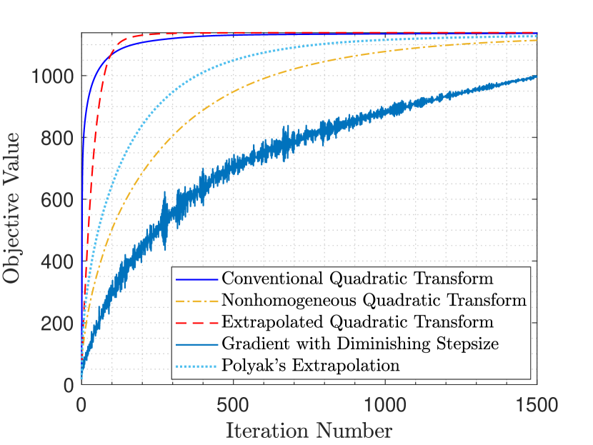
Figure 1: Solving the FP problem (3) in which $n=5$, $d=9$, $\ell=4$ each $\omega_{i}=1$, each $\mathcal{X}_{i}=\{\bm{X}\in\mathbb{C}^{d\times\ell}:\text{tr}(\bm{X}\bm{X}^{\mathrm{H}})\leq 10\}$, and each entry of $\bm{A}_{i}$ and $\bm{B}_{ij}$ drawn i.i.d. according to the complex Gaussian distribution $\mathcal{CN}(0,1)$; further, we add $\bm{I}$ to each matrix denominator to ensure positive definiteness. We plot the average convergence of the different algorithms over 100 random realizations. Figure (a) displays the convergence in iterations, while figure (b) displays the convergence in time.

Proposition 2

Algorithms 1 and 2 are both the MM methods. Algorithms 1, 2, and 3 all guarantee convergence to some stationary point of the FP problem 3.

We then analyze the rate of convergence for the various quadratic transform methods. Due to the nonconvexity of the FP problem, the global analysis (assuming that the starting point is far from any stationary point) is intractable. We would like to give a local analysis by restricting the constraint set to a small neighborhood of a strict local optimum (so that the starting point is not far away), i.e.,

$$\mathcal{X}=\big{\{}\underline{\bm{x}}:\|\underline{\bm{x}}-\underline{\bm{x}}^{*}\|_{2}\leq R\big{\}},$$ (21)

where $\underline{\bm{x}}^{*}$ is a strict local optimum of (3) satisfying

$$\nabla^{2}f_{o}(\underline{\bm{x}}^{*})\preceq-\xi\bm{I}\prec\mathbf{0}$$

for some strictly positive constant $\xi>0$, and the radius $R>0$ is sufficiently small so that $f_{o}(\underline{\bm{x}})$ is concave on $\mathcal{X}$. Assume that the Hessian of $f_{o}(\underline{\bm{x}})$ is $L$-Lipschitz continuous on $\mathcal{X}$, i.e.,

$$\|\nabla^{2}f_{o}(\underline{\bm{x}})-\nabla^{2}f_{o}(\underline{\bm{x}}^{\prime})\|_{2}\leq L\|\underline{\bm{x}}-\underline{\bm{x}}^{\prime}\|_{2}$$

for any $\underline{\bm{x}},\underline{\bm{x}}^{\prime}\in\mathcal{X}$. By Corollary 1.2.2 of [2], we have

$$\nabla^{2}f_{o}(\underline{\bm{x}})\preceq\nabla^{2}f_{o}(\underline{\bm{x}}^{*})+L\|\underline{\bm{x}}-\underline{\bm{x}}^{*}\|_{2}\bm{I},$$

so it suffices to require $R\leq\xi/L$ in order to ensure that $f_{o}(\underline{\bm{x}})$ is concave on $\mathcal{X}$.

The following analysis uses the MM interpretation in Proposition 2. Conditioned on $\underline{\bm{x}}^{\prime}\in\mathcal{X}$, define the gaps between $f_{o}(\underline{\bm{x}})$ and the two surrogate functions to be two functions of $\underline{\bm{x}}\in\mathcal{X}$ as

$$\delta_{q}(\underline{\bm{x}}|\underline{\bm{x}}^{\prime}) =f_{o}(\underline{\bm{x}})-f_{q}(\underline{\bm{x}},\mathcal{Y}(\underline{\bm{x}}^{\prime})),$$

$$\delta_{t}(\underline{\bm{x}}|\underline{\bm{x}}^{\prime}) =f_{o}(\underline{\bm{x}})-f_{t}(\underline{\bm{x}},\mathcal{Y}(\underline{\bm{x}}^{\prime}),\underline{\bm{x}}^{\prime}).$$

It can be readily shown that

$$\delta_{q}(\underline{\bm{x}}^{k}|\underline{\bm{x}}^{k})=\delta_{t}(\underline{\bm{x}}^{k}|\underline{\bm{x}}^{k})=0,$$ (22a)

$$\nabla\delta_{q}(\underline{\bm{x}}^{k}|\underline{\bm{x}}^{k})=\nabla\delta_{t}(\underline{\bm{x}}^{k}|\underline{\bm{x}}^{k})=\mathbf{0}.$$ (22b)

Moreover, define the two quantities:

$$\Lambda_{q} =\max_{\underline{\bm{x}}\in\mathcal{X}}\lambda_{1}\big{(}\nabla^{2}\delta_{q}(\underline{\bm{x}}|\underline{\bm{x}})\big{)},$$

$$\Lambda_{t} =\max_{\underline{\bm{x}}\in\mathcal{X}}\lambda_{1}\big{(}\nabla^{2}\delta_{t}(\underline{\bm{x}}|\underline{\bm{x}})\big{)}.$$

Recall each ratio $M_{i}(\underline{\bm{x}})$ is finite with nonsingular denominator matrix $\sum^{n}_{i=1}\bm{B}_{ij}\bm{x}_{j}\bm{x}^{\mathrm{H}}_{j}\bm{B}^{\mathrm{H}}_{ij}$, so each entry of $\underline{\bm{y}}$ is finite and hence each $\lambda_{1}(\bm{D}_{i})<\infty$ according to (8). As a result, $\lambda_{1}(\nabla^{2}_{\underline{\bm{x}}}f_{t}(\underline{\bm{x}},\underline{\bm{y}},\underline{\bm{z}})=-\max_{i}2\lambda_{1}(\bm{D}_{i})>-\infty$. Further, $\Lambda_{t}\leq\lambda_{1}(\nabla^{2}_{\underline{\bm{x}}}f_{o}(\underline{\bm{x}}))-\lambda_{1}(\nabla^{2}_{\underline{\bm{x}}}f_{t}(\underline{\bm{x}},\mathcal{Y}(\underline{\bm{x}}^{\prime}),\underline{\bm{x}}^{\prime}))<\infty$. Moreover, because $\nabla^{2}_{\underline{\bm{x}}}f_{t}(\underline{\bm{x}},\mathcal{Y}(\underline{\bm{x}}^{\prime}),\underline{\bm{x}}^{\prime})\preceq\nabla^{2}_{\underline{\bm{x}}}f_{o}(\underline{\bm{x}},\mathcal{Y}(\underline{\bm{x}}^{\prime}))$, we must have $\Lambda_{q}\leq\Lambda_{t}<\infty$. We are now ready to show the (local) convergence rates of Algorithm 1 and Algorithm 2.

Proposition 3 (Convergence Rates of Algorithm 1 and Algorithm 2)

For the FP problem (3), the local convergence rate of Algorithm 1 or Algorithm 2 is

$$f_{o}(\underline{\bm{x}}^{*})-f_{o}(\underline{\bm{x}}^{1}) \leq\frac{\Lambda R^{2}}{2}+\frac{LR^{3}}{6},$$ (23)

$$f_{o}(\underline{\bm{x}}^{*})-f_{o}(\underline{\bm{x}}^{k}) \leq\frac{2\Lambda R^{2}+2LR^{3}/3}{k+3},\;\text{for}\;k\geq 2,$$ (24)

where

$$\Lambda=\left\{\begin{array}[]{ll}\!\!\Lambda_{q}&\text{for Algorithm \ref{algorithm:QT}};\vspace{0.5em}\\ \!\!\Lambda_{t}&\text{for Algorithm \ref{algorithm:GQT}}.\\ \end{array}\right.$$ (25)

Proof:

See Appendix A. ∎

Because $0\leq\Lambda_{q}\leq\Lambda_{t}$, Algorithm 1 converges faster than Algorithm 2 in iterations according to Proposition 3. Notice that $\Lambda_{q}$ and $\Lambda_{t}$ in essence characterize how well their corresponding surrogate functions approximate the second-order profile of $f_{o}(\underline{\bm{x}})$. In the ideal case, the surrogate function and $f_{o}(\underline{\bm{x}})$ have exactly the same second-order profile so that $\Lambda=0$, then the objective-value error bound in Proposition 3 becomes

$$f_{o}(\underline{\bm{x}})-f_{o}(\underline{\bm{x}}^{k})\leq\frac{L}{6}\|\underline{\bm{x}}-\underline{\bm{x}}^{k-1}\|^{3}_{2},$$ (26)

which also holds for the cubically regularized Newton’s method due to Nesterov as shown in [2]. Equipped with the error bound (26), it immediately follows from Theorem 4.1.4 in [2] that

$$f_{o}(\underline{\bm{x}}^{*})-f_{o}(\underline{\bm{x}}^{1}) \leq\frac{LR^{3}}{6},$$ (27)

$$f_{o}(\underline{\bm{x}}^{*})-f_{o}(\underline{\bm{x}}^{k}) \leq\frac{LR^{3}}{2(1+k/3)^{2}},\;\text{for}\;k\geq 2.$$ (28)

We now show that the extrapolated quadratic transform method in Algorithm 3 can achieve fairly close to the ideal case stated in (27) and (28). Since Algorithm 2 is a gradient projection method and Algorithm 3 accelerates it by Nesterov’s extrapolation, we immediately obtain the following convergence rate from Proposition 6.2.1 of [31].

Proposition 4 (Convergence Rate of Algorithm 3)

Suppose that the gradient of $f_{o}(\underline{\bm{x}})$ is $C$-Lipschitz continuous and let $\lambda_{i}^{k}=1/(2C)$. Then Algorithm 3 yields

$$f(\underline{\bm{x}}^{*})-f(\underline{\bm{x}})\leq\frac{2C\cdot[f(\underline{\bm{x}}^{*})-f(\underline{\bm{x}}^{0})]}{(k+1)^{2}},\;\;\text{for}\;k\geq 1.$$ (29)

In summary, as compared to Algorithm 1 and Algorithm 2 that both yield an objective-value error bound of $O(1/k)$, Algorithm 3 yields a smaller error bound of $O(1/k^{2})$.

VI Other FP Problems

Our discussion thus far is limited to the sum-of-weighted-ratios FP problem in (3). The goal of this section is to extend the above results to the other FP problems. We now consider a general FP objective function

$$g_{o}(\underline{\bm{x}})=\mathcal{G}\big{(}M_{1}(\underline{\bm{x}}),\ldots,M_{n}(\underline{\bm{x}})\big{)}$$ (30)

in place of $f_{o}(\underline{\bm{x}})$ in problem (3), where $\mathcal{G}:\mathbb{R}^{n}\rightarrow\mathbb{R}$ is a differentiable function with $n$ ratio arguments.

Assume that $g_{o}(\underline{\bm{x}})$ can be bounded from below as

$$h(\underline{\bm{x}},\bm{t})=\sum^{n}_{i=1}\Big{[}\alpha_{i}(\bm{t})\cdot\hat{M}_{i}(\underline{\bm{x}})\Big{]}+\beta(\bm{t}),$$ (31)

where $\bm{t}$ is an auxiliary variable, $\alpha_{i}(\bm{t})\geq 0$, $i=1,\ldots,n$, and $\beta(\bm{t})$ are all differentiable scalar-valued functions of $\bm{t}$, and

$$\hat{M}_{i}(\underline{\bm{x}})=\big{(}\hat{\bm{A}}_{i}\bm{x}_{i}\big{)}^{\mathrm{H}}\Bigg{(}\sum^{n}_{j=1}\hat{\bm{B}}_{ij}\bm{x}_{j}\bm{x}_{j}^{\mathrm{H}}\hat{\bm{B}}_{ij}^{\mathrm{H}}\Bigg{)}^{-1}\big{(}\hat{\bm{A}}_{i}\bm{x}_{i}\big{)}.$$ (32)

Notice that $\hat{M}_{i}(\underline{\bm{x}})\neq M_{i}(\underline{\bm{x}})$ in general. Assume also that the lower bound is tight, i.e.,

$$g_{o}(\underline{\bm{x}})=\max_{\bm{t}}h(\underline{\bm{x}},\bm{t}).$$ (33)

The optimal value of the auxiliary variable $\bm{t}$ depends on what the current $\underline{\bm{x}}$ is, so it can be written as a function of $\underline{\bm{x}}$, i.e.,

$$\bm{t}^{\star}=\arg\max_{\bm{t}}h(\underline{\bm{x}},\bm{t})\triangleq\mathcal{T}(\underline{\bm{x}}).$$ (34)

A natural idea is to optimize $\underline{\bm{x}}$ and $\bm{t}$ alternatingly in the lower bound $h(\underline{\bm{x}},\bm{t})$. In particular, since the optimization of $\underline{\bm{x}}$ in $h(\underline{\bm{x}},\bm{t})$ under fixed $\bm{t}$ is a sum-of-weighed-ratios FP problem, the various quadratic transform methods can be readily applied.

Algorithm 4 Generalized Quadratic Transform

1:  Initialize $\underline{\bm{x}}$ to a feasible value.

2:  repeat

3:     Update $\bm{t}$ according to (34).

4:     Update $\underline{\bm{x}}$ by applying one iteration of Algorithm 1, or Algorithm 2, or Algorithm 3 to (31) for fixed $\bm{t}$.

5:  until the value of $f_{o}(\underline{\bm{x}})$ converges

The key observation is that updating $\bm{t}$ in (34) amounts to constructing a surrogate function for $g_{o}(\underline{\bm{x}})$; recall that the quadratic transform is also to construct a surrogate function. Thus, updating $t$ followed by one iteration of the quadratic transform method can be recognized as constructing a surrogate function of $g_{o}(\underline{\bm{x}})$ for the current $\underline{\bm{x}}$. In other words, after updating $\bm{t}$, we do not need to run the quadratic transform method (Algorithm 1, or Algorithm 2, or Algorithm 3) with the convergence reached in full; rather, we can just run one iteration of the quadratic transform method, and its convergence is guaranteed by the MM theory. Algorithm 4 summarizes the above method.

An interesting fact is that the connection with the gradient projection carries over to Algorithm 4, as stated in the following proposition.

Proposition 5

If Algorithm 2 is used in step 4 of Algorithm 4, then Algorithm 4 is equivalent to a gradient projection, i.e.,

$$\bm{x}^{k}_{i}=\mathcal{P}_{\mathcal{X}_{i}}\bigg{(}\bm{x}^{k-1}_{i}+c^{k}_{i}\cdot\frac{\partial g_{o}(\underline{\bm{x}}^{k-1})}{\partial\bm{x}^{c}_{i}}\bigg{)},$$ (35)

where $k=1,2,\ldots$ is the iteration index for the loop in Algorithm 4, and $c^{k}_{i}>0$ is the stepsize.

Proof:

See Appendix B. ∎

We now illustrate the result of Proposition 5 through a concrete example which was first proposed in [1] for the WSR problem. Consider the logarithmic FP problem

$$\underset{\underline{\bm{x}}}{\text{maximize}} \quad\sum^{n}_{i=1}\mu_{i}\log\big{(}1+M_{i}(\underline{\bm{x}})\big{)}$$ (36a)

subject to $$\quad\|\bm{x}_{i}\|^{2}_{2}\leq\rho,\;\text{for}\;i=1,\ldots,n,$$ (36b)

where each weight $\mu_{i}>0$. The above type of problem is extensively considered in the communication field.

By the Lagrangian dual transform [7], we can construct the surrogate function $h(\underline{\bm{x}},\bm{t})$ as

$$h(\underline{\bm{x}},\bm{t})=\sum^{n}_{i=1}\Big{[}\mu_{i}(1+t_{i})\cdot\hat{M}_{i}(\underline{\bm{x}})\Big{]}\\ +\sum^{n}_{i=1}\Big{[}\mu_{i}\log(1+t_{i})-\mu_{i}t_{i}\Big{]},$$ (37)

where

$$\hat{M}_{i}(\underline{\bm{x}})=\big{(}\bm{A}_{i}\bm{x}_{i}\big{)}^{\mathrm{H}}\Bigg{(}\bm{A}_{i}\bm{x}_{i}\bm{x}_{i}^{\mathrm{H}}\bm{A}_{i}^{\mathrm{H}}+\sum^{n}_{j=1}\bm{B}_{ij}\bm{x}_{j}\bm{x}_{j}^{\mathrm{H}}\bm{B}_{ij}^{\mathrm{H}}\Bigg{)}^{-1}\\ \big{(}\bm{A}_{i}\bm{x}_{i}\big{)}.$$ (38)

The corresponding new objective function $g_{t}(\underline{\bm{x}},\underline{\bm{y}},\underline{\bm{z}},\bm{t})$ by the nonhomogeneous quadratic transform is

$$g_{t}(\underline{\bm{x}},\underline{\bm{y}},\underline{\bm{z}},\bm{t})=\sum^{n}_{i=1}\Big{[}2\Re\big{\{}\mu_{i}(1+t_{i})\bm{x}^{\mathrm{H}}_{i}\bm{A}^{\mathrm{H}}_{i}\bm{y}_{i}$$

$$\qquad\quad+\bm{x}^{\mathrm{H}}_{i}(\hat{\lambda}_{i}\bm{I}-\hat{\bm{D}}_{i})\bm{z}_{i}\big{\}}+\bm{z}^{\mathrm{H}}_{i}(\hat{\bm{D}}_{i}-\hat{\lambda}_{i}\bm{I})\bm{z}_{i}-\hat{\lambda}_{i}\bm{x}^{\mathrm{H}}_{i}\bm{x}_{i}\Big{]}$$

$$\qquad\quad+\sum^{n}_{i=1}\Big{[}\mu_{i}\log(1+t_{i})-\mu_{i}t_{i}\Big{]},$$ (39)

where

$$\hat{\bm{D}}_{i}=\mu_{i}(1+t_{i})\bm{A}_{i}^{\mathrm{H}}\bm{y}_{i}\bm{y}_{i}^{\mathrm{H}}\bm{A}_{i}+\sum^{n}_{j=1}\mu_{j}(1+t_{j})\bm{B}_{ji}^{\mathrm{H}}\bm{y}_{j}\bm{y}^{\mathrm{H}}_{j}\bm{B}_{ji}.$$

The variables of $g_{t}(\underline{\bm{x}},\underline{\bm{y}},\underline{\bm{z}},\bm{t})$ in (VI) are optimized iteratively. First, by Lemma 2, each $\bm{z}_{i}$ is optimally determined as

$$\bm{z}^{\star}_{i}=\bm{x}_{i}.$$ (40)

By completing the square for each $\bm{y}_{i}$ in (VI), we obtain the optimal $\bm{y}_{i}$ as

$$\bm{y}_{i}^{\star} =\Bigg{(}\bm{A}_{i}\bm{x}_{i}\bm{x}_{i}^{\mathrm{H}}\bm{A}_{i}^{\mathrm{H}}+\sum^{n}_{i=1}\bm{B}_{ij}\bm{x}_{j}\bm{x}^{\mathrm{H}}_{j}\bm{B}^{\mathrm{H}}_{ij}\Bigg{)}^{-1}\bm{A}_{i}\bm{x}_{i}.$$ (41)

With the above $\bm{z}_{i}^{\star}$ and $\bm{y}_{i}^{\star}$ substituted in (VI), each optimal $t_{i}$ can be obtained as

$$t_{i}^{\star} =M_{i}(\underline{\bm{x}}).$$ (42)

Moreover, when $(\underline{\bm{y}},\underline{\bm{z}},\bm{t})$ are all held fixed, we complete the square for each $\bm{x}_{i}$ in $g_{t}(\underline{\bm{x}},\underline{\bm{y}},\underline{\bm{z}},\bm{t})$ and solve for $\bm{x}_{i}$ as

$$\bm{x}^{\star}_{i}=\left\{\begin{array}[]{ll}\!\!\hat{\bm{x}}_{i}&\text{if}\;\|\hat{\bm{x}}_{i}\|^{2}_{2}\leq\rho;\vspace{0.5em}\\ \!\!\big{(}\sqrt{\rho}/\|\hat{\bm{x}}_{i}\|_{2}\big{)}\hat{\bm{x}}_{i}&\text{otherwise},\end{array}\right.$$ (43)

where

$$\hat{\bm{x}}_{i}=\bm{z}_{i}+\frac{1}{\hat{\lambda}_{i}}\Big{(}\mu_{i}(1+t_{i})\bm{A}^{\mathrm{H}}_{i}\bm{y}_{i}-\hat{\bm{D}}_{i}\bm{z}_{i}\Big{)}.$$ (44)

Because $h(\underline{\bm{x}},\bm{t})$ in (37) meets the condition in Proposition 5, we have the following claim:

Corollary 1

For the logarithmic FP problem (36), updating $\underline{\bm{z}}$, $\underline{\bm{y}}$, $\bm{t}$, and $\underline{\bm{x}}$ respectively by (40), (41), (42), and (43) in an iterative fashion is equivalent to the gradient projection:

$$\bm{x}^{k}_{i}=\mathcal{P}_{\|\bm{x}_{i}\|^{2}_{2}\leq\rho}\bigg{(}\bm{x}^{k-1}_{i}+\frac{1}{\hat{\lambda}_{i}}\cdot\frac{\partial g_{o}(\underline{\bm{x}}^{k-1})}{\partial\bm{x}^{c}_{i}}\bigg{)},$$

where $g_{o}(\underline{\bm{x}})=\sum^{n}_{i=1}\mu_{i}\log\big{(}1+M_{i}(\underline{\bm{x}})\big{)}$.

Remark 3

In the above example, we treat each $\mu_{j}(1+t_{j})$ in (37) as the weight of the ratio $\hat{M}_{i}(\underline{\bm{x}})$, and then applying the conventional quadratic transform gives rise to the WMMSE algorithm [8, 9]. Alternatively, we could have let $\hat{M}_{i}(\underline{\bm{x}})$ absorb $\mu_{i}(1+t_{i})$ and then treat $\mu_{i}(1+t_{i})\hat{M}_{i}(\underline{\bm{x}})$ as the ratio term with weight one; [7] shows the above type of ratio term is more suited for the discrete FP solving. In fact, there are infinitely many ways of deciding which part is the ratio term and which part is the weight. The resulting quadratic transform method can be accelerated as in Algorithm 3, regardless.

 

$$f_{q}(\underline{\bm{X}},\underline{\bm{Y}}) =\sum^{n}_{i=1}\Bigg{[}\omega_{i}\cdot\mathrm{tr}\Bigg{(}\bm{X}^{\mathrm{H}}_{i}\bm{A}^{\mathrm{H}}_{i}\bm{Y}_{i}+\bm{Y}_{i}^{\mathrm{H}}\bm{A}_{i}\bm{X}_{i}-\bm{Y}^{\mathrm{H}}_{i}\Bigg{(}\sum^{n}_{j=1}\bm{B}_{ij}\bm{X}_{j}\bm{X}^{\mathrm{H}}_{j}\bm{B}^{\mathrm{H}}_{ij}\Bigg{)}\bm{Y}_{i}\Bigg{)}\Bigg{]}$$ (46)

 

$$f_{t}(\underline{\bm{X}},\underline{\bm{Y}},\underline{\bm{Z}})=\sum^{n}_{i=1}\Bigg{[}\mathrm{tr}\Big{(}\omega_{i}\bm{X}^{\mathrm{H}}_{i}\bm{A}^{\mathrm{H}}_{i}\bm{Y}_{i}+\omega_{i}\bm{Y}^{\mathrm{H}}_{i}\bm{A}_{i}\bm{X}_{i}+2\bm{X}^{\mathrm{H}}_{i}(\lambda_{i}\bm{I}-\bm{D}_{i})\bm{Z}_{i}+\bm{Z}^{\mathrm{H}}_{i}(\bm{D}_{i}-\lambda_{i}\bm{I})\bm{Z}_{i}-\lambda_{i}\bm{X}^{\mathrm{H}}_{i}\bm{X}_{i}\Big{)}\Bigg{]}$$ (50)

VII Matrix Ratio Case

This section extends the preceding results to the generalized matrix ratios with the matrix variables $\bm{X}_{i}\in\mathbb{C}^{d\times m}$ as in (4). The sum-of-weighted-ratios FP problem in (3) now becomes

$$\underset{\underline{\bm{X}}}{\text{maximize}} \quad\sum^{n}_{i=1}\Big{[}\omega_{i}\mathrm{tr}\big{(}\bm{M}_{i}(\underline{\bm{X}})\big{)}\Big{]}$$ (45a)

subject to $$\quad\bm{X}_{i}\in\mathcal{X}_{i},\;\text{for}\;i=1,\ldots,n.$$ (45b)

The new objective function $f_{q}(\underline{\bm{X}},\underline{\bm{Y}})$ by the quadratic transform is shown in (46), where an auxiliary variable $\bm{Y}_{i}\in\mathbb{C}^{d\times M}$ is introduced for each matrix ratio $\bm{M}_{i}(\underline{\bm{X}})$.

Optimizing $\underline{\bm{X}}$ and $\underline{\bm{Y}}$ alternatingly in $f_{q}(\underline{\bm{X}},\underline{\bm{Y}})$ leads us to the matrix-ratio version of Algorithm 1, wherein

$$\bm{Y}_{i}^{\star}=\Bigg{(}\sum^{n}_{i=1}\bm{B}_{ij}\bm{X}_{j}\bm{X}^{\mathrm{H}}_{j}\bm{B}^{\mathrm{H}}_{ij}\Bigg{)}^{-1}\big{(}\bm{A}_{i}\bm{X}_{i}\big{)}$$ (47)

and

$$\bm{X}^{\star}_{i}=\arg\min_{\bm{X}_{i}\in\mathcal{X}_{i}}\big{\|}\bm{D}^{\frac{1}{2}}_{i}\big{(}\bm{X}_{i}-\omega_{i}\bm{D}^{-1}_{i}\bm{A}^{\mathrm{H}}_{i}\bm{Y}_{i}\big{)}\big{\|}_{F}$$ (48)

with

$$\bm{D}_{i}=\sum^{n}_{j=1}\omega_{j}\bm{B}_{ji}^{\mathrm{H}}\bm{Y}_{j}\bm{Y}^{\mathrm{H}}_{j}\bm{B}_{ji}.$$ (49)

We further extend the new objective function $f_{t}(\underline{\bm{X}},\underline{\bm{Y}},\underline{\bm{Z}})$ of the nonhomogeneous quadratic transform as shown in (50), with an auxiliary variable $\bm{Z}_{i}\in\mathbb{C}^{d\times m}$ introduced for each $\bm{D}_{i}$. Again, we optimize the variables of $f_{t}(\underline{\bm{X}},\underline{\bm{Y}},\underline{\bm{Z}})$ in an iterative fashion: $\underline{\bm{Z}}$ is optimally updated to $\underline{\bm{X}}$, $\underline{\bm{Y}}$ is optimally updated as in (47), and $\underline{\bm{X}}$ is optimally updated as

$$\bm{X}_{i}^{\star} =\mathcal{P}_{\mathcal{X}_{i}}\bigg{(}\bm{Z}_{i}+\frac{1}{\lambda_{i}}\Big{(}\omega_{i}\bm{A}^{\mathrm{H}}_{i}\bm{Y}_{i}-\bm{D}_{i}\bm{Z}_{i}\Big{)}\bigg{)}.$$

Combining the above steps gives the matrix-ratio version of Algorithm 2. Its connection with the gradient projection continues to hold:

$$\bm{X}^{k}=\mathcal{P}_{\mathcal{X}_{i}}\bigg{(}\bm{X}^{k-1}_{i}+\frac{1}{2\lambda^{k}_{i}}\cdot\frac{\partial f_{o}(\underline{\bm{X}}^{k-1})}{\partial\bm{X}_{i}^{c}}\bigg{)}.$$ (51)

Equipped with (51), Algorithm 3 can be immediately extended to the matrix ratio case as well.

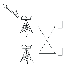
Figure 2: Two BSs serve one downlink user each. One BS performs ISAC while the other BS only performs transmission; the aim of sensing is to recover the angle $\theta$. The dashed arrows represent the interference.

VIII Two Application Cases

VIII-A ISAC

Consider two base-stations (BSs) as depicted in Fig. 2. BS 1 performs ISAC while BS 2 only performs downlink transmission. The two BSs have $M$ transmit antennas each, the two downlink users have $N$ antennas each, and BS 1 has $N_{r}$ radar receive antennas. Denote by $\bm{H}_{ij}\in\mathbb{C}^{N\times M}$ the channel from BS $j$ to downlink user $i$, where $i,j\in\{1,2\}$, $\bm{G}\in\mathbb{C}^{N_{r}\times M}$ the channel from BS 2 to the radar receiver at BS 1, $\sigma^{2}_{i}$ the background noise power at downlink user $i$, and $\sigma^{2}_{r}$ the background noise power at BS 1. Let $\bm{v}_{i}\in\mathbb{C}^{M}$ be the transmit precoder at BS $i$ subject to the power constraint $P_{\max}$, i.e., $\|\bm{v}_{i}\|^{2}_{2}\leq P_{\max}$.

 

$$f_{t}(\underline{\bm{v}},\underline{\bm{y}},\underline{\bm{z}}) =2\Re\Big{\{}\bm{v}^{\mathrm{H}}_{1}\Big{[}\alpha\dot{\bm{A}}^{\mathrm{H}}\bm{y}_{r}+\omega_{1}\bm{H}_{11}^{\mathrm{H}}\bm{y}_{1}+(\lambda_{1}\bm{I}-\bm{D}_{1})\bm{z}_{1}\Big{]}+\bm{v}^{\mathrm{H}}_{2}\Big{[}\omega_{2}\bm{H}_{22}^{\mathrm{H}}\bm{y}_{2}+(\lambda_{2}\bm{I}-\bm{D}_{2})\bm{z}_{2}\Big{]}\Big{\}}$$

$$\qquad\bm{z}^{\mathrm{H}}_{1}(\bm{D}_{1}-\lambda_{1}\bm{I})\bm{z}_{1}+\bm{z}^{\mathrm{H}}_{2}(\bm{D}_{2}-\lambda_{2}\bm{I})\bm{z}_{2}-\lambda_{1}\|\bm{v}_{1}\|^{2}_{2}-\lambda_{2}\|\bm{v}_{2}\|^{2}_{2}-\alpha\sigma^{2}_{r}\|\bm{y}_{r}\|^{2}_{2}-\omega_{1}\sigma^{2}_{1}\|\bm{y}_{1}\|^{2}_{2}-\omega_{2}\sigma^{2}_{2}\|\bm{y}_{2}\|^{2}_{2}$$ (63)

Moreover, for BS 1, consider the transmit steering vector $\bm{a}_{t}(\theta)\in\mathbb{C}^{M}$ and the receive steering vector $\bm{a}_{r}(\theta)\in\mathbb{C}^{N_{r}}$, both dependent on the target angle $\theta$ as shown in Fig. 2:

$$\bm{a}_{t}(\theta) =\big{[}1,e^{-j\pi\sin\theta},\ldots,e^{-j\pi(M-1)\sin\theta}\big{]}^{\top},$$

$$\bm{a}_{r}(\theta) =\big{[}1,e^{-j\pi\sin\theta},\ldots,e^{-j\pi(N_{r}-1)\sin\theta}\big{]}^{\top}.$$

Thus, for the complex Gaussian symbol $\bm{s}_{i}\sim\mathcal{CN}(\mathbf{0},\bm{I})$ from BS $i\in\{1,2\}$, the received echo signal at BS 1 is given by

$$r=\xi\bm{a}_{r}(\theta)\bm{a}_{t}(\theta)^{\top}\bm{v}_{1}\bm{s}_{1}+\bm{G}\bm{v}_{2}\bm{s}_{2}+\bm{z},$$ (52)

where $\xi\in\mathbb{C}$ is the reflection coefficient, and $\bm{z}\sim\mathcal{CN}(\mathbf{0},\sigma^{2}_{r}\bm{I})$ is the background noise at BS 1. Let $\hat{\bm{F}}=\bm{G}\bm{v}_{2}\bm{s}_{2}+\bm{z}$ and define the interference-plus-noise covariance matrix to be

$$\bm{Q}=\mathbb{E}[\hat{\bm{F}}\hat{\bm{F}}^{\text{H}}]=\sigma^{2}_{r}\bm{I}+\bm{G}\bm{v}_{2}\bm{v}_{2}^{\mathrm{H}}\bm{G}^{\mathrm{H}}.$$ (53)

The Fisher information about the target angle $\theta$ in Fig. 2 is then computed as

$$J_{\theta}=\alpha\bm{v}_{1}^{\mathrm{H}}\dot{\bm{A}}^{\mathrm{H}}\bm{Q}^{-1}\dot{\bm{A}}\bm{v}_{1},$$ (54)

where $\bm{A}=\bm{a}_{r}(\theta)\bm{a}_{t}(\theta)^{\top}$, $\dot{\bm{A}}=\partial\bm{A}/\partial\theta$, and $\alpha=2|\xi|^{2}$. The SINRs of the two downlink users are given by

$$\mathrm{SINR}_{1} =\bm{v}_{1}^{\mathrm{H}}\bm{H}_{11}^{\mathrm{H}}\Big{(}\sigma^{2}_{1}\bm{I}+\bm{H}_{12}\bm{v}_{2}\bm{v}_{2}^{\mathrm{H}}\bm{H}_{12}^{\mathrm{H}}\Big{)}^{-1}\bm{H}_{11}\bm{v}_{1},$$ (55)

$$\mathrm{SINR}_{2} =\bm{v}_{2}^{\mathrm{H}}\bm{H}_{22}^{\mathrm{H}}\Big{(}\sigma^{2}_{2}\bm{I}+\bm{H}_{21}\bm{v}_{1}\bm{v}_{1}^{\mathrm{H}}\bm{H}_{21}^{\mathrm{H}}\Big{)}^{-1}\bm{H}_{22}\bm{v}_{2}.$$ (56)

We seek the optimal precoders $\underline{\bm{v}}=\{\bm{v}_{1},\bm{v}_{2}\}$ to maximize a linear combination of the Fisher information (for the sensing purpose) and the two SINRs (for the communication purpose):

$$\underset{\underline{\bm{v}}}{\text{maximize}} \quad J_{\theta}+\omega_{1}\mathrm{SINR}_{1}+\omega_{2}\mathrm{SINR}_{2}$$ (57a)

subject to $$\quad\|\bm{v}_{i}\|^{2}_{2}\leq P_{\max},\;\;i\in\{1,2\},$$ (57b)

where $\omega_{i}>0$ reflects the priority of $\mathrm{SINR}_{i}$ as compared to $J_{\theta}$ in the ISAC task.

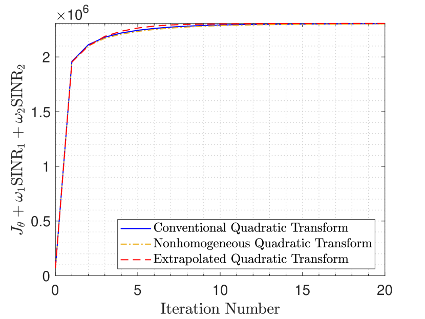
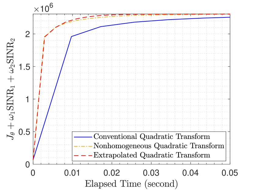
Figure 3: Maximizing a weighted sum of Fisher information and SINRs in the ISAC problem. Figure (a) shows the convergence in iterations, while figure (b) shows the convergence in time.

By the conventional quadratic transform, the original objective function can be recast to

$$f_{q}(\underline{\bm{v}},\underline{\bm{y}})=2\Re\{\alpha\bm{v}_{1}^{\mathrm{H}}\dot{\bm{A}}^{\mathrm{H}}\bm{y}_{r}\}-\alpha\bm{y}_{r}^{\mathrm{H}}\Big{(}\sigma^{2}_{r}\bm{I}+\bm{G}\bm{v}_{2}\bm{v}_{2}^{\mathrm{H}}\bm{G}^{\mathrm{H}}\Big{)}\bm{y}_{r}$$

$$\;+2\Re\{\omega_{1}\bm{v}_{1}^{\mathrm{H}}\bm{H}_{11}^{\mathrm{H}}\bm{y}_{1}\}-\omega_{1}\bm{y}_{1}^{\mathrm{H}}\Big{(}\sigma^{2}_{1}\bm{I}+\bm{H}_{12}\bm{v}_{2}\bm{v}_{2}^{\mathrm{H}}\bm{H}_{12}^{\mathrm{H}}\Big{)}\bm{y}_{1}$$

$$\;+2\Re\{\omega_{2}\bm{v}_{2}^{\mathrm{H}}\bm{H}_{22}^{\mathrm{H}}\bm{y}_{2}\}-\omega_{2}\bm{y}_{2}^{\mathrm{H}}\Big{(}\sigma^{2}_{2}\bm{I}+\bm{H}_{21}\bm{v}_{1}\bm{v}_{1}^{\mathrm{H}}\bm{H}_{21}^{\mathrm{H}}\Big{)}\bm{y}_{2},$$ (58)

where the auxiliary variables $\bm{y}_{r}\in\mathbb{C}^{N_{r}}$, $\bm{y}_{1}\in\mathbb{C}^{N}$, and $\bm{y}_{2}\in\mathbb{C}^{N}$ are introduced for $J_{\theta}$, $\mathrm{SINR}_{1}$, and $\mathrm{SINR}_{2}$, respectively. We optimize the precoders $\underline{\bm{v}}$ and the auxiliary variables $\underline{\bm{y}}=(\bm{y}_{r},\bm{y}_{1},\bm{y}_{2})$ alternatingly as

$$\underline{\bm{v}}^{0}\rightarrow\cdots\rightarrow\underline{\bm{v}}^{k-1}\rightarrow\underline{\bm{y}}^{k}\rightarrow\underline{\bm{v}}^{k}\rightarrow\cdots.$$

When $\underline{\bm{v}}$ is held fixed, all the auxiliary variables can be optimally determined for $f_{q}(\underline{\bm{v}},\underline{\bm{y}})$ in closed form as

$$\bm{y}_{r}^{\star} =\Big{(}\sigma^{2}_{r}\bm{I}+\bm{G}\bm{v}_{2}\bm{v}_{2}^{\mathrm{H}}\bm{G}^{\mathrm{H}}\Big{)}^{-1}\dot{\bm{A}}\bm{v}_{1},$$ (59a)

$$\bm{y}_{1}^{\star} =\Big{(}\sigma^{2}_{1}\bm{I}+\bm{H}_{12}\bm{v}_{2}\bm{v}_{2}^{\mathrm{H}}\bm{H}_{12}^{\mathrm{H}}\Big{)}^{-1}\bm{H}_{11}\bm{v}_{1},$$ (59b)

$$\bm{y}_{2}^{\star} =\Big{(}\sigma^{2}_{2}\bm{I}+\bm{H}_{21}\bm{v}_{1}\bm{v}_{1}^{\mathrm{H}}\bm{H}_{21}^{\mathrm{H}}\Big{)}^{-1}\bm{H}_{22}\bm{v}_{2}.$$ (59c)

After the update of the auxiliary variables, we find the optimal $\underline{\bm{v}}$ in closed form as

$$\bm{v}_{1}^{\star} =\Big{(}\eta_{1}\bm{I}+\bm{D}_{1}\Big{)}^{-1}\Big{(}\alpha\dot{\bm{A}}^{H}\bm{y}_{r}+\omega_{1}\bm{H}_{11}^{\mathrm{H}}\bm{y}_{1}\Big{)},$$ (60a)

$$\bm{v}_{2}^{\star} =\Big{(}\eta_{2}\bm{I}+\bm{D}_{2}\Big{)}^{-1}\omega_{2}\bm{H}_{22}^{\mathrm{H}}\bm{y}_{2},$$ (60b)

where

$$\bm{D}_{1} =\omega_{2}\bm{H}_{21}^{\mathrm{H}}\bm{y}_{2}\bm{y}_{2}^{\mathrm{H}}\bm{H}_{21},$$ (61a)

$$\bm{D}_{2} =\alpha\bm{G}^{\mathrm{H}}\bm{y}_{r}\bm{y}_{r}^{\mathrm{H}}\bm{G}+\omega_{1}\bm{H}_{12}^{\mathrm{H}}\bm{y}_{1}\bm{y}_{1}^{\mathrm{H}}\bm{H}_{12},$$ (61b)

and the Lagrange multipliers $(\eta_{1},\eta_{2})$ for the power constraint are optimally determined as

$$\eta_{i}^{\star}=\min\big{\{}\eta_{i}\geq 0:\|\bm{v}_{i}\|^{2}_{2}\leq P_{\max}\big{\}}.$$ (62)

To implement (62) in practice, we may first try out $\eta^{\star}_{i}=0$ to see if $\|\bm{v}_{i}\|^{2}_{2}\leq P_{\max}$; if not, then we further tune $\eta^{\star}$ via bisection search to render $\|\bm{v}_{i}\|^{2}_{2}=P_{\max}$.

Differing from the above conventional quadratic transform, the nonhomogeneous quadratic transform recasts the original objective function (57a) to $f_{t}(\underline{\bm{v}},\underline{\bm{y}},\underline{\bm{z}})$ as shown in (VIII-A). Again, we optimize the variables in $f_{t}(\underline{\bm{v}},\underline{\bm{y}},\underline{\bm{z}})$ iteratively as

$$\underline{\bm{v}}^{0}\rightarrow\cdots\rightarrow\underline{\bm{v}}^{k-1}\rightarrow\underline{\bm{z}}^{k}\rightarrow\underline{\bm{y}}^{k}\rightarrow\underline{\bm{v}}^{k}\rightarrow\underline{\bm{z}}^{k+1}\rightarrow\cdots.$$

When $\underline{\bm{v}}$ and $\underline{\bm{y}}$ are both held fixed, $\underline{\bm{z}}$ is optimally updated as $\bm{z}_{1}^{\star}=\bm{v}_{1}$, and $\bm{z}_{2}^{\star}=\bm{v}_{2}$. The optimal update of $\underline{\bm{y}}$ is the same as in (59a), (59b), and (59c). When $\underline{\bm{y}}$ and $\underline{\bm{z}}$ are both held fixed, we first compute

$$\hat{\bm{v}}_{1}=\bm{z}_{1}+\frac{1}{\lambda_{1}}\Big{(}\alpha\dot{\bm{A}}^{\mathrm{H}}\bm{y}_{r}+\omega_{1}\bm{H}_{11}^{\mathrm{H}}\bm{y}_{1}-\bm{D}_{1}\bm{z}_{1}\Big{)}$$ (64)

and

$$\hat{\bm{v}}_{2}=\bm{z}_{2}+\frac{1}{\lambda_{2}}\Big{(}\omega_{2}\bm{H}_{22}^{\mathrm{H}}\bm{y}_{2}-\bm{D}_{2}\bm{z}_{2}\Big{)},$$ (65)

and then update $\underline{\bm{v}}$ optimally as

$$\bm{v}^{\star}_{i}=\left\{\begin{array}[]{ll}\!\!\hat{\bm{v}}_{i}&\text{if}\;\|\hat{\bm{v}}_{i}\|^{2}_{2}\leq P_{\max};\vspace{0.5em}\\ \!\!\big{(}\sqrt{P_{\max}}/\|\hat{\bm{v}}_{i}\|_{2}\big{)}\hat{\bm{v}}_{i}&\text{otherwise}.\end{array}\right.$$ (66)

We validate the performance of the various quadratic transform methods in Fig. 3. In our simulation case, $M=64$, $N=2$, $N_{r}=72$, $\omega_{1}=\omega_{2}=10^{5}$, $\sigma_{1}^{2}=\sigma_{2}^{2}=-80$ dBm, $\sigma_{r}^{2}=-80$ dBm, and $P_{\max}=20$ dBm. The path loss (in dB) is computed as $32.6+36.7\log_{10}d$, where $d$ is the distance in meters; the position coordinates of BS 1, BS 2, user 1, user 2, and the sensed object are $(0,0)$, $(250,0)$, $(-10,100)$, $(350,100)$, and $(200,200)$, respectively, all in meters. The Rayleigh fading model is adopted. Algorithm 1, Algorithm 2, and Algorithm 3 are tested. As shown in Fig. 2(a), if the convergence is considered in terms of iterations, then all these algorithms yield almost the same convergence rate. The objective value is monotonically increasing with the iteration number by all these algorithms. If we instead evaluate convergence in terms of the elapsed time as displayed in Fig. 2(b), then the proposed two accelerated methods, Algorithm 2 and Algorithm 3, become much faster than Algorithm 1; the former two algorithms attain convergence after 0.02 seconds, whereas the latter algorithm still does not converge after 0.05 seconds. Algorithm 3 outperforms Algorithm 2, but their gap is marginal.

VIII-B Massive MIMO

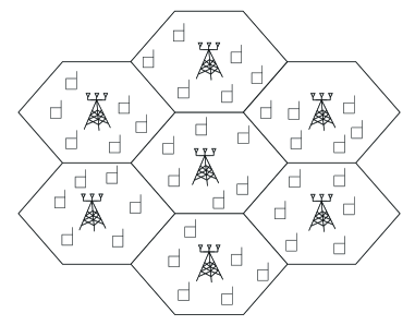
Figure 4: A 7-cell wrapped-around massive MIMO network.

The application case of massive MIMO is closely related to the example stated in Section VI. Consider a downlink multi-cell network with $L$ cells as depicted in Fig. 4. In each cell, one BS with $M$ antennas sends independent messages towards $Q$ downlink user terminals simultaneously by spatial multiplexing; it shall be well understood that $Q\leq M$. Assume also that each user terminal has $N$ receive antennas. In particular, $M\gg N$ under the massive MIMO setting.

Moreover, we use $\ell,i=1,\ldots,L$ to index the cells and the corresponding BSs, and use $q,j=1,\ldots,Q$ to index the users in each cell. Denote by $\bm{H}_{\ell q,i}\in\mathbb{C}^{N\times M}$ the channel from BS $i$ to the $q$th user in cell $\ell$, denote by $\bm{v}_{\ell q}\in\mathbb{C}^{M}$ the transmit precoder of BS $\ell$ for its $q$th associated user, and denote by $\sigma^{2}$ the background noise power. The SINR of the $q$th user in cell $\ell$, denoted by $\mathrm{SINR}_{\ell q}$, is computed as

$$\mathrm{SINR}_{\ell q}=\bm{v}_{\ell q}^{\mathrm{H}}\bm{H}_{\ell q,\ell}^{\mathrm{H}}\Bigg{(}\sigma^{2}\bm{I}+\sum_{(i,j)\neq(\ell,q)}\bm{H}_{\ell q,i}\bm{v}_{ij}\bm{v}_{ij}^{\mathrm{H}}\bm{H}_{\ell q,i}^{\mathrm{H}}\Bigg{)}\\ \bm{H}_{\ell q,\ell}\bm{v}_{\ell q}.$$ (67)

Assigning a positive weight $\mu_{\ell q}>0$ for each user $q$ in cell $\ell$, we seek the optimal set of precoding vectors $\underline{\bm{v}}=\{\bm{v}_{\ell q}\}$ to maximize the weighted sum-of-rates throughout the network:

$$\underset{\underline{\bm{v}}}{\text{maximize}} \quad\sum^{L}_{\ell=1}\sum^{Q}_{q=1}\mu_{\ell q}\log\big{(}1+\mathrm{SINR}_{\ell q}\big{)}$$ (68a)

subject to $$\quad\sum^{Q}_{q=1}\|\bm{v}_{\ell q}\|^{2}_{2}\leq P_{\max},\;\text{for}\;\ell=1,\ldots,L,$$ (68b)

where the constraint (68b) states that the total transmit power at each BS cannot exceed the power budget $P_{\max}$.

The traditional WMMSE method [8, 9] addresses the above problem by performing the following iterative updates:

$$\underline{\bm{v}}^{0}\rightarrow\cdots\rightarrow\underline{\bm{v}}^{k-1}\rightarrow\underline{\bm{y}}^{k}\rightarrow\bm{t}^{k}\rightarrow\underline{\bm{v}}^{k}\rightarrow\cdots,$$

where the auxiliary variable $\bm{t}$ is updated as

$$t^{\star}_{\ell q}=\mathrm{SINR}_{\ell q}$$ (69)

for the current $\underline{\bm{v}}$, and the auxiliary variable $\underline{\bm{y}}$ is updated as

$$\bm{y}^{\star}_{\ell q} =\Bigg{(}\sigma^{2}\bm{I}+\sum^{L}_{i=1}\sum^{Q}_{j=1}\bm{H}_{\ell q,i}\bm{v}_{ij}\bm{v}^{\mathrm{H}}_{ij}\bm{H}^{\mathrm{H}}_{\ell q,i}\Bigg{)}^{-1}\bm{H}_{\ell q,\ell}\bm{v}_{\ell q}.$$ (70)

With the auxiliary variables held fixed, the precoding vectors are optimally updated as

$$\bm{v}_{\ell q}(\eta_{\ell})=\Bigg{(}\eta_{\ell}\bm{I}+\sum^{L}_{i=1}\sum^{Q}_{j=1}\mu_{ij}(1+t_{ij})\bm{H}^{\mathrm{H}}_{ij,\ell}\bm{y}_{ij}\bm{y}^{\mathrm{H}}_{ij}\bm{H}_{ij,\ell}\Bigg{)}^{-1}\\ \mu_{\ell q}(1+t_{\ell q})\bm{H}^{\mathrm{H}}_{\ell q,\ell}\bm{y}_{\ell q},$$ (71)

where the Lagrange multiplier $\eta_{\ell}$ accounts for the power constraint at BS $\ell$ and is optimally determined as

$$\eta_{\ell}^{\star}=\min\Bigg{\{}\eta\geq 0:\sum^{Q}_{q=1}\|\bm{v}_{\ell q}(\eta)\|^{2}_{2}\leq P_{\max}\Bigg{\}}.$$ (72)

In the practical implementation, the above $\eta_{\ell}$ can be obtained via bisection search; an $M\times M$ matrix inverse needs to be computed in (71) for each bisection search iterate, which can be quite costly because $M\gg N$.

In contrast, the nonhomogeneous quadratic transform reformulates the objective function as

$$g_{t}(\underline{\bm{v}},\underline{\bm{y}},\underline{\bm{z}},\bm{t})=\sum^{L}_{\ell=1}\sum^{Q}_{q=1}\Big{[}2\Re\big{\{}\mu_{\ell q}(1+t_{\ell q})\bm{v}^{\mathrm{H}}_{\ell q}\bm{H}^{\mathrm{H}}_{\ell q,\ell}\bm{y}_{\ell q}$$

$$\,+\bm{v}^{\mathrm{H}}_{\ell q}(\hat{\lambda}_{\ell}\bm{I}-\hat{\bm{D}}_{\ell})\bm{z}_{\ell q}\big{\}}+\bm{z}^{\mathrm{H}}_{\ell q}(\hat{\bm{D}}_{\ell}-\hat{\lambda}_{\ell}\bm{I})\bm{z}_{\ell q}-\hat{\lambda}_{\ell}\bm{v}^{\mathrm{H}}_{\ell q}\bm{v}_{\ell q}$$

$$\,-\mu_{\ell q}(1+t_{\ell q})\sigma^{2}\bm{y}_{\ell q}^{\mathrm{H}}\bm{y}_{\ell q}+\mu_{\ell q}\log(1+t_{\ell q})-\mu_{\ell q}t_{\ell q}\Big{]},$$ (73)

for which the iterative updates are carried out as

$$\underline{\bm{v}}^{0}\rightarrow\cdots\rightarrow\underline{\bm{v}}^{k-1}\rightarrow\underline{\bm{z}}^{k}\rightarrow\underline{\bm{y}}^{k}\rightarrow\bm{t}^{k}\rightarrow\underline{\bm{v}}^{k}\rightarrow\cdots,$$

where the auxiliary variable $\underline{\bm{z}}$ is updated as $\bm{z}_{iq}=\bm{v}_{iq}$, and the other two auxiliary variables $\underline{\bm{y}}$ and $\bm{t}$ are updated as in (70) and (69), respectively. To update $\underline{\bm{v}}$, we first compute

$$\hat{\bm{v}}_{\ell q}=\bm{z}_{\ell q}+\frac{1}{\hat{\lambda}_{\ell}}\Big{(}\mu_{\ell q}(1+t_{\ell q})\bm{H}^{\mathrm{H}}_{\ell q,\ell}\bm{y}_{\ell q}-\hat{\bm{D}}_{\ell}\bm{z}_{\ell q}\Big{)},$$ (74)

where

$$\hat{\bm{D}}_{\ell}=\sum^{L}_{i=1}\sum^{Q}_{j=1}\mu_{ij}(1+t_{ij})\bm{H}_{ij,\ell}^{\mathrm{H}}\bm{y}_{ij}\bm{y}^{\mathrm{H}}_{ij}\bm{H}_{ij,\ell},$$ (75)

and then incorporate the power constraint as

$$\bm{v}^{\star}_{\ell q}=\left\{\begin{array}[]{ll}\!\!\hat{\bm{v}}_{\ell q}&\text{if}\;\sum^{Q}_{j=1}\|\hat{\bm{v}}_{\ell j}\|^{2}_{2}\leq P_{\max};\vspace{0.5em}\\ \!\!\sqrt{\frac{{P_{\max}}}{\sum^{Q}_{j=1}\|\hat{\bm{v}}_{\ell j}\|^{2}_{2}}}\hat{\bm{v}}_{\ell q}&\text{otherwise}.\end{array}\right.$$

As opposed to the updating formula (71) of the WMMSE algorithm, the update of $\underline{\bm{v}}$ in Algorithm 2 no longer incurs any matrix inverse. Even though Algorithm 2 still requires computing matrix inverse for updating the auxiliary variable $\underline{\bm{y}}$ as in (70), the matrix size is just $N\times N$ with $N\ll M$ and thus can be neglected. Moreover, the above beamforming method for massive MIMO can be accelerated via extrapolation as in Algorithm 3.

We now test the various quadratic transform methods for massive MIMO in a simulated 7-hexagonal-cell wrapped-around network as considered in [3]. Within each cell, the BS is located at the center and the $6$ downlink users are randomly placed. Each BS has $128$ antennas and each user has $4$ antennas. The BS-to-BS distance is set to be $0.8$ km. The maximum transmit power level at the BS side is set to be $20$ dBm, and the AWGN power level is set to be $-90$ dBm. The downlink distance-dependent path-loss is simulated by $128.1+37.6\log_{10}(d)+\tau$ (in dB), where $d$ represents the BS-to-user distance in km, and $\tau$ is a zero-mean Gaussian random variable with $8$ dB standard deviation for the shadowing effect. We consider sum rate maximization by setting all the weights to $1$. Again, Algorithm 1, Algorithm 2, and Algorithm 3 are the competitors. As shown in Fig. 5(a), Algorithm 1 converges faster than the other two methods in terms of iterations; this result agrees with the former discussion below Proposition 3. When it comes to the convergence evaluated by time, as shown in Fig. 5(b), the two accelerated quadratic transform methods are much more efficient than the conventional method in Algorithm 1. In particular, observe that Algorithm 3 is also much faster than Algorithm 2, as opposed to the ISAC case in Fig. 2. There are two reasons. First, there are more matrix ratio terms in the massive MIMO problem case; second, the FP of massive MIMO has a more complicated structure (with ratios nested in logarithms). When MPF contains more ratios or has a more complicated structure, the surrogate function approximation by the nonhomogeneous quadratic transform tends to be loose, in which case Nesterov’s extrapolation becomes more effective.

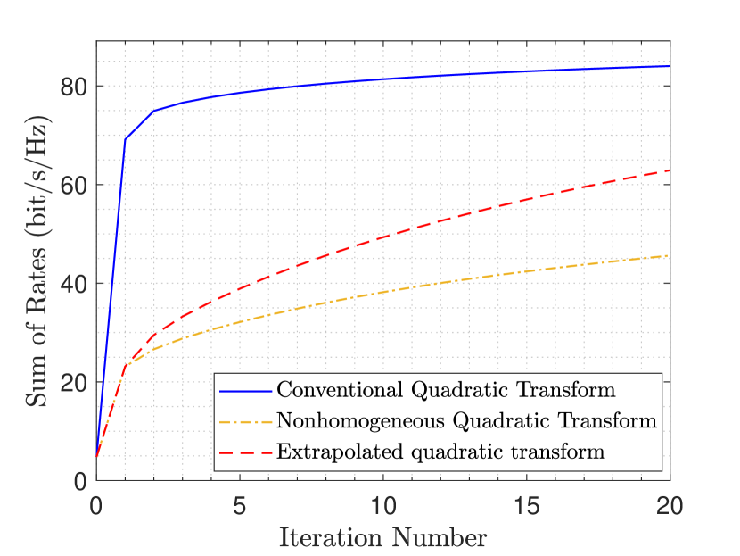
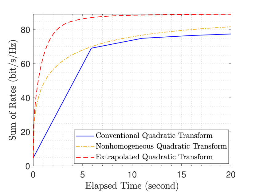
Figure 5: Maximizing the sum of rates in a multi-cell downlink massive MIMO network. Figure (a) shows the convergence in iterations, while figure (b) shows the convergence in time.

IX Conclusion

This work considerably develops the existing theory and algorithm of FP, focusing on their applications in wireless networks. The quadratic transform is a state-of-the-art tool in the FP area. As a starting point, we establish a connection between the quadratic transform and the gradient projection; this connection turns out to be fairly useful in that it enables the iterative optimization to get rid of matrix inverses. We then propose further accelerating the quadratic transform via extrapolation. Of fundamental importance is the convergence rate analysis that follows. To the best of our knowledge, this is the very first work that examines how fast the quadratic transform (including its special case the WMMSE algorithm) converges and also how to render it even faster. Moreover, we demonstrate the practical usefulness of the accelerated quadratic transform through two application cases, ISAC and massive MIMO, both of which are envisioned to be the key components of the next-generation wireless networks.

Appendix A
Proof of Proposition 3

We focus on the convergence rate of Algorithm 1; the convergence rate of Algorithm 2 can be established similarly. Lemma 1.2.4 in [2] states that for any twice-differentiable function $f(\bm{x})$ with $L$-Lipschitz continuous gradient, we have

$$\bigg{|}f(\bm{x}^{\prime})-f(\bm{x})-\nabla f(\bm{x})^{\mathrm{H}}(\bm{x}^{\prime}-\bm{x})\\ -\frac{1}{2}(\bm{x}^{\prime}-\bm{x})^{\mathrm{H}}\nabla^{2}f(\bm{x})(\bm{x}^{\prime}-\bm{x})\bigg{|}\leq\frac{L}{6}\|\bm{x}^{\prime}-\bm{x}\|^{3}_{2}$$

given any two feasible $\bm{x}$ and $\bm{x}^{\prime}$. Applying the above lemma to the function $\delta_{q}(\underline{\bm{x}}|\underline{\bm{x}}^{k-1})$ and using the results in (22) give

$$\quad\;\frac{L}{6}\|\underline{\bm{x}}-\underline{\bm{x}}^{k-1}\|^{3}_{2}$$

$$\geq\delta_{q}(\underline{\bm{x}}|\underline{\bm{x}}^{k-1})$$

$$\quad-\frac{1}{2}(\underline{\bm{x}}-\underline{\bm{x}}^{k-1})^{\mathrm{H}}\nabla^{2}\delta_{q}(\underline{\bm{x}}^{k-1}|\underline{\bm{x}}^{k-1})(\underline{\bm{x}}-\underline{\bm{x}}^{k-1})$$

$$\geq\delta_{q}(\underline{\bm{x}}|\underline{\bm{x}}^{k-1})-\frac{\Lambda_{q}}{2}\|\underline{\bm{x}}-\underline{\bm{x}}^{k-1}\|^{2}_{2}$$

$$=f_{o}(\underline{\bm{x}})-f_{q}(\underline{\bm{x}},\underline{\bm{y}}^{k})-\frac{\Lambda_{q}}{2}\|\underline{\bm{x}}-\underline{\bm{x}}^{k-1}\|^{2}_{2}$$

$$\overset{(a)}{\geq}f_{o}(\underline{\bm{x}})-f_{q}(\underline{\bm{x}}^{k},\underline{\bm{y}}^{k})-\frac{\Lambda_{q}}{2}\|\underline{\bm{x}}-\underline{\bm{x}}^{k-1}\|^{2}_{2}$$

$$\overset{(b)}{\geq}f_{o}(\underline{\bm{x}})-f_{q}(\underline{\bm{x}}^{k},\underline{\bm{y}}^{k+1})-\frac{\Lambda_{q}}{2}\|\underline{\bm{x}}-\underline{\bm{x}}^{k-1}\|^{2}_{2}$$

$$\overset{(c)}{=}f_{o}(\underline{\bm{x}})-f_{o}(\underline{\bm{x}}^{k})-\frac{\Lambda_{q}}{2}\|\underline{\bm{x}}-\underline{\bm{x}}^{k-1}\|^{2}_{2},$$ (76)

where step $(a)$ follows since $\underline{\bm{x}}^{k}$ maximizes $f_{q}(\underline{\bm{x}},\underline{\bm{y}})$ for the current $\underline{\bm{y}}=\underline{\bm{y}}^{k}$, step $(b)$ follows since $\underline{\bm{y}}^{k+1}$ maximizes $f_{q}(\underline{\bm{x}},\underline{\bm{y}})$ for the current $\underline{\bm{x}}=\underline{\bm{x}}^{k}$, and step $(c)$ follows by the property of the surrogate function. Following Nesterov’s proof technique in [2], we let

$$\underline{\bm{x}}=\pi\underline{\bm{x}}^{*}+(1-\pi)\underline{\bm{x}}^{k-1},$$ (77)

where the parameter $\pi\in[0,1]$. Then the concavity of $f_{o}(\underline{\bm{x}})$ on $\mathcal{X}$ gives

$$f_{o}(\underline{\bm{x}})\leq\pi f_{o}(\underline{\bm{x}}^{*})+(1-\pi)f_{o}(\underline{\bm{x}}^{k-1}).$$ (78)

Denote the gap in the objective value as

$$v_{k}=f_{o}(\underline{\bm{x}}^{*})-f_{o}(\underline{\bm{x}}^{k}).$$ (79)

Substituting (77) and (78) into (76) gives rise to

$$v_{k} \leq(1-\pi)v_{k-1}+\frac{\pi^{2}\Lambda_{q}}{2}\|\underline{\bm{x}}-\underline{\bm{x}}^{k-1}\|^{2}_{2}$$

$$\qquad+\frac{\pi^{3}L}{6}\|\underline{\bm{x}}-\underline{\bm{x}}^{k-1}\|^{3}_{2}$$

$$\leq(1-\pi)v_{k-1}+\pi^{2}\bigg{(}\frac{\Lambda_{q}R^{2}}{2}+\frac{LR^{3}}{6}\bigg{)},$$ (80)

where the second inequality follows by (21) and $0\leq\pi\leq 1$. The choice of $\pi$ depends on $k$.

When $k=1$, we let $\pi=1$ in (80) and obtain

$$v_{1}\leq\frac{\Lambda_{q}R^{2}}{2}+\frac{LR^{3}}{6}.$$ (81)

When $k\geq 2$, we let

$$\pi=\frac{v_{k-1}}{\Lambda_{q}R^{2}+LR^{3}/3}.$$ (82)

It can be shown by induction that the above $\pi$ is always feasible (i.e., $0\leq\pi\leq 1$) for all $k\geq 2$. Plugging (82) in (80) yields

$$v_{k}\leq v_{k-1}\bigg{(}1-\frac{v_{k-1}}{2\Lambda_{q}R^{2}+2LR^{3}/3}\bigg{)},$$ (83)

which can be further rewritten as

$$\frac{1}{v_{k}} \geq\frac{1}{v_{k-1}}\cdot\bigg{(}1-\frac{v_{k-1}}{2\Lambda_{q}R^{2}+2LR^{3}/3}\bigg{)}^{-1}$$

$$\geq\frac{1}{v_{k-1}}\cdot\bigg{(}1+\frac{v_{k-1}}{2\Lambda_{q}R^{2}+2LR^{3}/3}\bigg{)}$$

$$=\frac{1}{v_{k-1}}+\frac{1}{2\Lambda_{q}R^{2}+2LR^{3}/3},$$ (84)

where the second inequality follows since $(1-a)^{-1}>1+a$ for any $0\leq a\leq 1$. The result of (84) immediately gives

$$\frac{1}{v_{k}} \geq\frac{1}{v_{1}}+\frac{k-1}{2\Lambda_{q}R^{2}+2LR^{3}/3}$$

$$\geq\frac{k+3}{2\Lambda_{q}R^{2}+2LR^{3}/3},$$ (85)

where the second inequality is due to (81). The proof is then completed for Algorithm 1. The case of Algorithm 2 can be verified similarly.

Appendix B
Proof of Proposition 5

Because optimizing $\bm{t}$ in (34) for fixed $\underline{\bm{x}}$ is an unconstrained differentiable problem, the optimal $\bm{t}^{\star}$ must satisfy the first-order condition

$$\frac{d\beta(\bm{t}^{\star})}{d\bm{t}}+\sum^{n}_{j=1}\bigg{[}\frac{d\alpha_{j}(\bm{t}^{\star})}{d\bm{t}}\cdot\hat{M}_{j}(\underline{\bm{x}})\bigg{]}=0,$$ (86)

in light of which the partial derivative of $g_{o}(\underline{\bm{x}})$ can be considerably simplified as

$$\frac{\partial g_{o}(\underline{\bm{x}})}{\partial\bm{x}^{c}_{i}} =\frac{\partial h(\underline{\bm{x}},\mathcal{T}(\underline{\bm{x}}))}{\partial\bm{x}^{c}_{i}}$$

$$=\sum^{n}_{j=1}\bigg{[}\frac{d\alpha_{j}(\bm{t}^{\star})}{d\bm{t}}\frac{\partial\mathcal{T}(\underline{\bm{x}})}{\partial\bm{x}^{c}_{i}}\hat{M}_{j}(\underline{\bm{x}})+\alpha_{j}(\bm{t}^{\star})\frac{\partial\hat{M}_{j}(\underline{\bm{x}})}{\partial\bm{x}^{c}_{i}}\bigg{]}$$

$$\qquad+\frac{d\beta(\bm{t}^{\star})}{d\bm{t}}\frac{\partial\mathcal{T}(\underline{\bm{x}})}{\partial\bm{x}^{c}_{i}}$$

$$=\sum^{n}_{j=1}\bigg{[}\alpha_{j}(\bm{t}^{\star})\frac{\partial\hat{M}_{j}(\underline{\bm{x}})}{\partial\bm{x}^{c}_{i}}\bigg{]}.$$ (87)

We now apply to $h(\underline{\bm{x}},\bm{t})$ the nonhomogeneous quadratic transform in Section III-B, and thus obtain the new objective function

$$g_{t}(\underline{\bm{x}},\underline{\bm{y}},\underline{\bm{z}},\bm{t})=\sum^{n}_{i=1}\Big{[}2\Re\big{\{}\alpha_{i}(\bm{t})\bm{x}^{\mathrm{H}}_{i}\bm{A}^{\mathrm{H}}_{i}\bm{y}_{i}+\bm{x}^{\mathrm{H}}_{i}(\hat{\lambda}_{i}\bm{I}-\hat{\bm{D}}_{i})\bm{z}_{i}\big{\}}\\ +\bm{z}^{\mathrm{H}}_{i}(\hat{\bm{D}}_{i}-\hat{\lambda}_{i}\bm{I})\bm{z}_{i}-\hat{\lambda}_{i}\bm{x}^{\mathrm{H}}_{i}\bm{x}_{i}\Big{]}+\beta(\bm{t}),$$ (88)

where

$$\hat{\bm{D}}_{i}=\sum^{n}_{j=1}\alpha_{j}(\bm{t})\hat{\bm{B}}_{ji}^{\mathrm{H}}\bm{y}_{j}\bm{y}^{\mathrm{H}}_{j}\hat{\bm{B}}_{ji}$$ (89)

and

$$\hat{\lambda}_{i}\geq\lambda_{\max}(\hat{\bm{D}}_{i}).$$ (90)

We optimize the variables $(\underline{\bm{x}},\underline{\bm{y}},\underline{\bm{z}},\bm{t})$ iteratively as

$$\underline{\bm{x}}^{0}\rightarrow\cdots\rightarrow\underline{\bm{x}}^{k-1}\rightarrow\underline{\bm{z}}^{k}\rightarrow\underline{\bm{y}}^{k}\rightarrow\bm{t}^{k}\rightarrow\underline{\bm{x}}^{k}\rightarrow\cdots.$$

The optimal update of $\bm{x}^{k}_{i}$ is

$$\bm{x}^{k}_{i} \overset{(a)}{=}\mathcal{P}_{\mathcal{X}_{i}}\bigg{(}\bm{x}^{k-1}_{i}+\frac{1}{\hat{\lambda}_{i}^{k}}\Big{(}\alpha_{i}(\bm{t}^{k})\hat{\bm{A}}^{\mathrm{H}}_{i}\bm{y}^{k}_{i}-\hat{\bm{D}}^{k}_{i}\bm{x}^{k-1}_{i}\Big{)}\bigg{)}$$

$$\overset{(b)}{=}\mathcal{P}_{\mathcal{X}_{i}}\Bigg{(}\bm{x}_{i}^{k-1}+\frac{1}{2\hat{\lambda}_{i}^{k}}\sum^{n}_{j=1}\Bigg{[}\alpha_{j}(\bm{t}^{k})\frac{\partial\hat{M}_{j}(\underline{\bm{x}}^{k-1})}{\partial\bm{x}^{c}_{i}}\Bigg{]}\Bigg{)},$$ (91)

where step $(a)$ follows since each $\bm{z}_{i}^{k}$ has been updated to $\bm{x}_{i}^{k-1}$, and step $(b)$ follows by Lemma 1. Substituting (87) in the above equation completes the proof.

References

- [1] Z. Zhang, Z. Zhao, K. Shen, D. P. Palomar, and W. Yu, “Discerning and enhancing the weighted sum-rate maximization algorithms in communications,” Nov. 2023, [Online]. Available: https://arxiv.org/pdf/2311.04546.
- [2] Y. Nesterov, “Lectures on convex optimization (second edition).” Springer, 2018.
- [3] K. Shen and W. Yu, “Fractional programming for communication systems—Part I: Power control and beamforming,” IEEE Trans. Signal Process., vol. 66, no. 10, pp. 2616–2630, Mar. 2018.
- [4] K. Shen, W. Yu, L. Zhao, and D. P. Palomar, “Optimization of MIMO device-to-device networks via matrix fractional programming: A minorization–maximization approach,” IEEE/ACM Trans. Netw., vol. 27, no. 5, pp. 2164–2177, Oct. 2019.
- [5] M. Razaviyayn, M. Hong, and Z.-Q. Luo, “A unified convergence analysis of block successive minimization methods for nonsmooth optimization,” SIAM J. Optim., vol. 23, no. 2, pp. 1126–1153, 2013.
- [6] Y. Sun, P. Babu, and D. P. Palomar, “Majorization-minimization algorithms in signal processing, communications, and machine learning,” IEEE Trans. Signal Process., vol. 65, no. 3, pp. 794–816, Aug. 2016.
- [7] K. Shen and W. Yu, “Fractional programming for communication systems—Part II: Uplink scheduling via matching,” IEEE Trans. Signal Process., vol. 66, no. 10, pp. 2631–2644, Mar. 2018.
- [8] S. S. Christensen, R. Agarwal, E. D. Carvalho, and J. M. Cioffi, “Weighted sum-rate maximization using weighted MMSE for MIMO-BC beamforming design,” IEEE Trans. Wireless Commun., vol. 7, no. 12, pp. 4792–4799, Dec. 2008.
- [9] Q. Shi, M. Razaviyayn, Z.-Q. Luo, and C. He, “An iteratively weighted MMSE approach to distributed sum-utility maximization for a MIMO interfering broadcast channel,” IEEE Trans. Signal Process., vol. 59, no. 9, pp. 4331–4340, Apr. 2011.
- [10] I. M. Stancu-Minasian, Fractional programming: Theory, methods and applications. Norwell, MA, USA: Kluwer, 2012.
- [11] A. Charnes and W. W. Cooper, “Programming with linear fractional functionals,” Nav. Res. Logist., vol. 9, no. 3, pp. 181–186, Dec. 1962.
- [12] S. Schaible, “Parameter-free convex equivalent and dual programs of fractional programming problems,” Zeitschrift für Oper. Res., vol. 18, no. 5, pp. 187–196, Oct. 1974.
- [13] W. Dinkelbach, “On nonlinear fractional programming,” Manage. Sci., vol. 13, no. 7, pp. 492–498, Mar. 1967.
- [14] J. P. Crouzeix, J. A. Ferland, and S. Schaible, “An algorithm for generalized fractional programs,” J. Optim. Theory Appl., vol. 47, no. 1, pp. 35–49, Sep. 1985.
- [15] R. W. Freund and F. Jarre, “Solving the sum-of-ratios problem by an interior-point method,” J. Global Optim., vol. 19, no. 1, pp. 83–102, Jan. 2001.
- [16] N. T. H. Phuong and H. Tuy, “A unified monotonic approach to generalized linear fractional programming,” J. Global Optim., vol. 26, pp. 229–259, July 2003.
- [17] H. Konno and K. Fukaishi, “A branch and bound algorithm for solving low rank linear multiplicative and fractional programming problems,” J. Global Optim., vol. 18, pp. 283–299, Nov. 2000.
- [18] H. P. Benson, “Global optimization of nonlinear sums of ratios,” J. Math. Anal. Appl., vol. 263, no. 1, pp. 301–315, Nov. 2001.
- [19] S. Qu, K. Zhang, and J. Zhao, “An efficient algorithm for globally minimizing sum of quadratic ratios problem with nonconvex quadratic constraints,” Appl. Math. Comput., vol. 189, no. 2, pp. 1624–1636, June 2007.
- [20] T. Kuno, “A branch-and-bound algorithm for maximizing the sum of several linear ratios,” J. Global Optim., vol. 22, pp. 155–174, Jan. 2002.
- [21] X. Liu, Y. Gao, B. Zhang, and F. Tian, “A new global optimization algorithm for a class of linear fractional programming,” MDPI Mathematics, vol. 7, no. 9, p. 867, Sep. 2019.
- [22] H. P. Benson, “Solving sum of ratios fractional programs via concave minimization,” J. Optim. Theory Appl., vol. 135, no. 1, pp. 1–17, June 2007.
- [23] ——, “Global optimization algorithm for the nonlinear sum of ratios problem,” J. Optim. Theory Appl., vol. 112, pp. 1–29, Jan. 2002.
- [24] ——, “Using concave envelopes to globally solve the nonlinear sum of ratios problem,” J. Global Optim., vol. 22, pp. 343–364, Jan. 2002.
- [25] K. Shen, H. V. Cheng, X. Chen, Y. C. Eldar, and W. Yu, “Enhanced channel estimation in massive MIMO via coordinated pilot design,” IEEE Trans. Commun., vol. 68, no. 11, pp. 6872–6885, Nov. 2020.
- [26] Y. Chen, L. Zhao, and K. Shen, “Mixed max-and-min fractional programming for wireless networks,” May 2023, [Online]. Available: https://arxiv.org/pdf/2305.02704.
- [27] X. Zhao, S. Lu, Q. Shi, and Z.-Q. Luo, “Rethinking WMMSE: Can its complexity scale linearly with the number of bs antennas?” IEEE Trans. Signal Process., vol. 71, pp. 433–446, Feb. 2023.
- [28] K. Zhou, Z. Chen, G. Liu, and Z. Chen, “A novel extrapolation technique to accelerate WMMSE,” in Proc. IEEE Int. Conf. Acoust., Speech, Signal Process. (ICASSP), June 2023.
- [29] A. Hjørungnes and D. Gesbert, “Complex-valued matrix differentiation: Techniques and key results,” IEEE Trans. Signal Process., vol. 55, no. 6, pp. 2740–2746, May 2007.
- [30] B. T. Polyak, “Some methods of speeding up the convergence of iteration methods,” USSR Computational Mathematics and Mathematical Physics, vol. 4, no. 5, pp. 1–17, 1964.
- [31] D. P. Bertsekas, “Convex optimization algorithms.” Athena Scientific, 2015.