Schrödinger’s control and estimation paradigm
with spatio-temporal distributions on graphs

Abstract

The problem of reconciling a prior probability law with data was introduced by E. Schrödinger in 1931/32. It represents an early formulation of a maximum likelihood problem. The specific formulation can also be seen as the control problem to modify the law of a diffusion process so as to match specifications on marginal distributions at given times. Thereby, in recent years, this so-called Schrödinger Bridge problem has been at the center of the development of uncertainty control. However, an unstudied facet of this program has been to address uncertainty in space and time, modeling the effect of tasks being completed, instead of imposing specifications at fixed times. The present work is a first study to extend Schrödinger’s paradigm on such an issue. It is developed in the context of Markov chains and random walks on graphs. Specifically, we study the case where one marginal distribution represents the initial state occupation of a Markov chain, while others represent first-arrival time distributions at absorbing states signifying completion of tasks. We establish that when the prior is Markov, a Markov policy is once again optimal with respect to a likelihood cost that follows Schrödinger’s dictum.

Stochastic control, random walks, large deviation theory, stopping times

1 Introduction

In a 1931/32 study [1, 2] E. Schrödinger asked for the most likely evolution of particles between two points in time where their distribution is observed. In this, he laid out elements of a large-deviations (LD) theory for the first time. Indeed, at a time when much of probability theory was in its infancy, and H. Cramer’s and I.N. Sanov’s theorems [3],[4] were still a few years away, Schrödinger single-handedly formulated and solved a maximum likelihood problem that is now known as the Schrödinger Bridge problem (SB problem) [5].

Schrödinger’s paradigm was slow to make inroads into probability theory until about the 1970s with the work of Jamison, Föllmer and others [6, 7, 8, 9, 10]. Since then it has become an integral part of stochastic control, fueling the recent fast development of uncertainty control – a discipline that focuses on regulating the uncertainty profiles of dynamical systems during operation as well as at some terminal time[11, 12, 13, 14, 15, 16, 17].

In contrast to this earlier literature where the typical control task is to bring the system to the vicinity of target states at some specified times, we are interested in regulating the times when target states are reached. Thereby, we introduce a new angle to Schrödinger’s dictum in which we now seek to reconcile stopping-time probability distributions instead of state-marginal distributions at predetermined points in time.

Interestingly, first-passage time statistics grew indispensable in modeling natural processes such as in the integrate-and-fire neuron models [18], bacterial steering via switching [19] and the chemical transport in active molecular processes [20]. A natural next step is to regulate the first-passage statistics via suitable control. For instance, in congestion control, specifying a uniform first-arrival time distribution of agents at the entrance of a site may be of practical use. In another instance, in landing a space probe, the distribution at landing is of essence whereas the precise time of landing may be random. Indeed, the full spectrum of such problems remains to be worked out.

In the present work, we explore such issues for a controlled random walk on a network. Time and space are discrete, namely, values for the time variable $\tau$ belong to some specified finite window $[1,t]\subset\mathbb{N}$ while the position $X_{\tau}$ at time $\tau$ of a random walker takes values on the vertex set $\mathcal{V}$ of a finite directed graph $\mathcal{G}$. The control authority entails altering prior transition probabilities for transferring between states so as to regulate the distribution of first-arrival (stopping) times at absorbing states over the given time window.

We identify the control cost with the value of a likelihood functional in observing a collection of random walkers as they traverse the network to match specifications on first arrivals. Thereby, we frame the control problem as a large deviations problem, in the spirit of Schrödinger’s approach. Remarkably, the solution to our problem takes the form of a Markov law, where control action is based on current information, as in the classical SB problem but for entirely different reasons.

The structure of the paper is as follows. In Section 2, we bring our setting closer to the reader by framing an example of De Moivre’s martingale as an SB with stopping-time marginals. In Section 3, we introduce notation and preliminaries. In Section 4, we delve into an important quality of the classical SBs and, remarkably, of the proposed variant of SB with stopping times, that the posterior law preserves the Markovianity of the prior in both problems. An explicit construction of the solution to modify the prior so as to match specifications on arrival probabilities is provided in Section 5. The analogy between both the estimation and control perspectives is highlighted in Section 6. Section 7 provides academic examples, including De Moivre’s martingale, to elucidate the application of the framework. The paper concludes with a brief discussion in Section 8 on generalizations and potential future directions.

2 De Moivre’s Martingale

We begin our exposition with a motivating example, De Moivre’s martingale which models a gambler’s ruin in a betting game with two stopping conditions [21]. The betting problem involves gamblers reaching a set amount before terminating the gambling game. This model problem distinguishes between the two possible outcomes, success in reaching the goal, or ruin where all the capital is lost. Now imagine that we observe a series of game rounds. In each round, one either wins the bet and increases their current wealth by one token or loses with the opposite effect. Assume the game begins with a set of players having initial wealth distributed on a finite set ${\mathcal{V}_{\rm trs}}=\{1,\ldots,M-1\}$ of values for the corresponding number of tokens, according to an initial distribution $\mu_{0}$. If a player loses all the capital or achieves a cap of cumulative $M$ tokens in any number of rounds, they discontinue the game. We presume our prior law corresponds to a fair game.

Over a discrete window of time $[1,t]\subset\mathbb{N}$, we observe the distribution of players that terminate the game for the above reasons, reaching the goal of $M$ tokens, or due to being ruined by hitting the lower bound $0$. These two distributions are denoted by $\hat{\nu}^{\rm win}(\tau),\hat{\nu}^{\rm ruin}(\tau)$, for $\tau\in[1,t]$, respectively. However, these observed time marginals may not be consistent with the prior law, leading us to suspect foul play. Thus, we seek to identify the most likely perturbation of the prior law that may explain the observed marginals and point to suspect times when foul play may have taken place.

We model this setting via a Markov chain with two absorbing states representing $0$ and $M$ tokens. This Markov chain has a total of $|{\mathcal{V}_{\rm trs}}|+2$ states. The problem being addressed is to determine the most likely law on trajectories that begin at time $0$ with the initial distribution on ${\mathcal{V}_{\rm trs}}$ and gives rise to the recorded time marginals. This example is revisited at the end of the paper after a theory in the spirit of Schrödinger for matching spatio-temporal marginal distributions is in place.

3 Notation and Rudiments on Large Deviations

Consider a directed finite graph $\mathcal{G}=(\mathcal{V},\mathcal{E})$, with vertex set $\mathcal{V}$ and edge set $\mathcal{E}$. We use $x,y\in\mathcal{V}$ to denote nodes, and often adjoin time $\tau\in\mathbb{Z}_{+}$ as a subscript $x_{\tau}\in\mathcal{V}$ to combine space-time indexing. We consider random walks $(X_{\tau})$ on $\mathcal{G}$ with absorbing vertices (states), and time $\tau\in[0,t]\subset\mathbb{Z}_{+}$, where $t$ is typically a bound on times we consider. We denote by ${\mathcal{V}_{\rm abs}}$ the set containing all absorbing vertices, and by ${\mathcal{V}_{\rm trs}}:=\mathcal{V}\setminus{\mathcal{V}_{\rm abs}}$ its complement of transient vertices. The framework may be readily modified to blend the two sets, via time-varying priors, but for simplicity, we will adhere to the assumption that these two sets of states are separate.

Thus, the probability space $\Omega$ that we consider for the random walk is discrete and finite. We typically use the symbols $Q,P$ to denote probability laws (and $L_{N}$ for empirical law of $N$ samples), while we reserve lowercase Greek letters such as $\mu,\nu$ for marginal distributions and $\pi,\Pi$ for transition probability matrices, e.g., $\pi(x,y)=Q(y|x)$, whereas $Q(\omega)$, $Q(x,y)$, and $Q(\mathcal{S})$ denote the probability of an outcome, joint probability ($\omega=(x,y)$), and probability of an event (set) $\mathcal{S}$, respectively. Vectors and matrices will be indexed, when needed, e.g., in $\Pi_{\tau}(x,y)$ with subscript denoting time.

Throughout we let $|{\mathcal{V}_{\rm abs}}|=m$ and $|{\mathcal{V}_{\rm trs}}|=n$. The initial occupation probability of the random walk will be denoted by

$$\mu_{0}(x_{0})=P(X_{0}=x_{0}),$$

for $x_{0}\in\mathcal{V}$ where, for simplicity, we assume that the support of $\mu_{0}$ is restricted to ${\mathcal{V}_{\rm trs}}$, that is,

$$\mu_{0}({\mathcal{V}_{\rm abs}})=0.$$

Next, we consider times when the random walk first arrives at a node $j$ in ${\mathcal{V}_{\rm abs}}$,

$$T_{j}:=\inf\{\tau>0\mid X_{\tau}=j\in{\mathcal{V}_{\rm abs}}\}.$$

Such times represent the completion of a task and are random, they are stopping times, with $X_{\tau}=j\in{\mathcal{V}_{\rm abs}}$ being the stopping criterion. We will be concerned with suitably adjusting the prior law to match specified marginal distributions for stopping times, which will typically be denoted $\nu_{j}(\tau)$, with subscript the absorbing state $j\in{\mathcal{V}_{\rm abs}}$.

In general, a probability law $P$ is said to be absolutely continuous with respect to $Q$, and denoted by $Q\gg P$, when $Q(\omega)=0$ implies that $P(\omega)=0$ for any $\omega\in\Omega$. Alternatively, we also say that the support of $Q$ contains the support of $P$. The Kullback-Leibler divergence between two laws $P,Q$, also known as relative entropy [22, 23], is defined by

$$\mathbb{D}(P\|Q):=\left\{\begin{array}[]{ll}\sum\limits_{\omega\in\Omega}P(\omega)\log\displaystyle\frac{P(\omega)}{Q(\omega)},&\mbox{when }Q\gg P,\\[8.0pt] \infty,&\mbox{otherwise},\end{array}\right.$$ (3)

where $0\cdot\log 0:=0$. It represents a distance between the two laws that quantifies how likely it is to observe an empirical distribution when sampling from a given law, as expressed by the following fundamental result of large deviations theory.

Theorem 3.1

(Sanov’s Theorem [23, 24]) Let $\mathbf{x}_{1},\ldots\mathbf{x}_{N}$ be independent identically distributed (i.i.d.) random vectors taking values in $\mathcal{X}$ with $|\mathcal{X}|<\infty$ and law $Q(\mathbf{x})$. For any set $\Gamma$ of probability distributions on $\mathcal{X}$ that is closed with nonempty interior,

$$\lim_{N\to\infty}-\frac{1}{N}\log Q^{N}(L_{N}\in\Gamma)=\mathbb{D}(P^{\star}\|Q),$$

where $P^{\star}=\arg\min_{P\in\Gamma}\mathbb{D}(P\|Q)$.

In layman’s terms, skipping a technicality in involving $\Gamma$, Sanov’s theorem states that the likelihood of observing an empirical distribution $L_{N}$ decays exponentially fast with the number of samples $N$, in that

$$Q^{N}(L_{N})\approx e^{-N\mathbb{D}(L_{N}\|Q)},$$

up to a suitable normalizing factor. Thus, the rate function $\mathbb{D}(\cdot\|\cdot)$ quantifies the likelihood of rare events, and the most likely event out of all the rare events that agree with a “neighborhood” $\Gamma$ of $L_{N}$, is the one having least divergence from the prior $\mathbb{D}(\cdot\|Q)$.

It is notable that the insights provided by Sanov’s result can be traced to the work of Schrödinger [1, 2]; indeed, in much the same way, Schrödinger discretized the path-space trajectories of Brownian particles to arrive at the most likely law that is consistent with observed marginal distributions – the classical Schrödinger bridge problem.

In closing, we also note that a much-heralded property of the classical Schrödinger bridges, is that the posterior retains the Markovian character of the prior. In general, there is no a priori guarantee for the posterior to retain features of the prior, such as Markovianity. Yet, as we will explain and contrast next, for entirely different reasons than in classical SBs, this is also the case for our problem where we constrain first-absorption time marginals. Having a Markovian law that ensures time marginals essentially allows such constraints to be achieved by active control since transitions can be decided based on the current state of the process.

4 On Markovian structure of posteriors

As a prelude to a key property of our problem, we provide a simple derivation of the same property of the classical Schrödinger Bridges, that when the prior is Markov, so is the posterior. While this property for SBs is standard and underlies the fact that density control can be effected by state feedback [25, Section 3], [14], [5], in the present situation where we design for distribution on first-arrival times, the Markov property for the posterior is far from obvious.

We proceed to show the reasons behind the Markovian property for each case. To this end, we consider paths

$$\mathbf{x}:=(x_{0},x_{1},\ldots,x_{t-1},x_{t})$$ (4)

over the finite time-window $[0,t]\subset\mathbb{N}$, taking values from the vertex set $\mathcal{V}$ as before, and denote by $Q({x_{0},x_{1},\ldots,x_{t}})$ the prior probability law. The law $Q$, or any other law, is Markov if and only if it factors as

$$Q({x_{0},x_{1},\ldots,x_{t-1},x_{t}})=q_{1}({x_{0},x_{1}})\times\cdots\times q_{t}({x_{t-1},x_{t}}),$$ (5)

for any suitably chosen factors. We are not concerned with interpreting the factors as conditional probabilities, as this is secondary at this point. For our purposes, it is only important that the law factors as the product of successive rank-$2$ tensors.

4.1 Classical SBs

In the classical SBs, one seeks the posterior $P^{\star}$ as

$$P^{\star}=\arg\min_{P}\sum_{\mathbf{x}\in\mathcal{V}^{t+1}}P(\mathbf{x})\log\frac{P(\mathbf{x})}{Q(\mathbf{x})},$$ (6a)

subject to

$$\sum_{x_{1},\ldots x_{t}\in\mathcal{V}}P(x_{0},x_{1},\ldots,x_{t-1},x_{t}) =\hat{\mu}_{0}{(x_{0})},$$ (6b)

$$\sum_{x_{0},\ldots x_{t-1}\in\mathcal{V}}P(x_{0},x_{1},\ldots,x_{t-1},x_{t}) =\hat{\mu}_{t}{(x_{t})}.$$ (6c)

Here, and throughout all similar optimization problems, we assume that the conditions are feasible (here (6b) and (6c)) and thereby that strong duality holds. Introducing Lagrange multipliers, we have the Lagrangian
$\displaystyle\mathcal{L}_{\rm SB}(P,\Lambda_{0},\Lambda_{t}):=\sum_{x_{0},\ldots,x_{t}\in\mathcal{V}}\bigg{[}$ $\displaystyle P(x_{0}\ldots,x_{t})\log\frac{P(x_{0},\ldots,x_{t})}{Q(x_{0}\ldots,x_{t})}$ $\displaystyle+$ $\displaystyle\Lambda_{0}(x_{0})\big{(}P(x_{0},\ldots,x_{t})-\hat{\mu}_{0}(x_{0})\big{)}$ $\displaystyle+$ $\displaystyle\Lambda_{t}(x_{t})\big{(}P(x_{0},\ldots,x_{t})-\hat{\mu}_{t}(x_{t})\big{)}\bigg{]}.$
The summation of $\Lambda_{0}(x_{0})P(x_{0},\ldots,x_{t})$ can be re-written as

$$\sum_{i_{0}\in\mathcal{V}}\sum_{x_{0},\ldots,x_{t}\in\mathcal{V}}\Lambda_{0}(i_{0})P(x_{0},\ldots,x_{t})\mathds{1}_{x_{0}=i_{0}}(x_{0},\ldots,x_{t}),$$

and similarly for the other summand, where $\mathds{1}_{\cdot}(\cdot)$ denotes the characteristic (Dirac) function. The minimizer takes the form

$$\begin{split}P^{\star}(x_{0},x_{1},\ldots,x_{t})&=Q(x_{0},x_{1},\ldots,x_{t})\times e^{-1}\\ &\times\scalebox{0.9}{\mbox{$\displaystyle\exp{\left[-\sum_{i_{0}\in\mathcal{V}}\Lambda_{0}(i_{0})\mathds{1}_{x_{0}=i_{0}}(x_{0},x_{1},\ldots,x_{t})\right]}$}}\\ &\times\scalebox{0.9}{\mbox{$\displaystyle\exp{\left[-\sum_{i_{t}\in\mathcal{V}}\Lambda_{t}(i_{t})\mathds{1}_{x_{t}=i_{t}}(x_{0},x_{1},\ldots,x_{t})\right]}$}}.\end{split}$$ (7)

Now note that

$$e^{-\sum_{i_{0}}\Lambda_{0}(i_{0})\mathds{1}_{x_{0}=i_{0}}(x_{0},x_{1},\ldots,x_{t})}=e^{-\Lambda_{0}(x_{0})},$$

and similarly, that

$$e^{-\sum_{i_{t}}\Lambda_{0}(i_{t})\mathds{1}_{x_{t}=i_{t}}(x_{0},x_{1},\ldots,x_{t})}=e^{-\Lambda_{t}(x_{t})}.$$

Thus, $P^{\star}(x_{0},x_{1}\ldots,x_{t})$ is expressed as the product

$$Q(x_{0},x_{1},\ldots,x_{t})\times\underbrace{f_{1}(x_{0},x_{1})\times\cdots\times f_{t}(x_{t-1},x_{t})}_{F(x_{0},\ldots,x_{t})},$$ (8)

where $f_{1}(x_{0},\cdot)=e^{-\Lambda_{0}(x_{0})-1}$ and $f_{t}(\cdot,x_{t})=e^{-\Lambda_{t}(x_{t})}$ are rank-$1$ (since their value depends on one index) and all other factors are trivially equal to $1$. Our choice to display the factorization of the “correction” tensor $F$ in full, serves to draw a parallel and contrast to what follows in the next subsection. This provides a rather transparent derivation of the following well-known result that can be traced to its continuous counterpart [1], [2] pertaining to diffusion processes.

Theorem 4.1

Assume that $Q$ is Markov and that the optimization problem with objective (6a) subject to (6b) and (6c) is feasible. Then, the (unique due to convexity) solution $P^{\star}$ is also Markov.

Proof 4.2.

Since the constraints are affine and the objective strictly convex, strong duality holds and the solution is in the form indicated in (7), and therefore in the follow-up expression (8). The product of tensors in the factored form $q({x_{0},x_{1}})\times\ldots\times q({x_{t-1},x_{t}})$ and $f_{0}(x_{0},x_{1})\times\ldots\times f_{t}(x_{t-1},x_{t})$, is again a tensor of the same form, i.e., a product of successive rank-$2$ tensors. Hence, the probability law $P^{\star}$ is Markov.

4.2 SBs with Absorbing States

Our new SB-type problem aims to reconcile marginals for random variables that are of a different nature. Specifically, these are marginals of $X_{0}$ and of the stopping times $T_{j}$ of the random walk at the absorbing states $j\in{\mathcal{V}_{\rm abs}}$. Thus, the support of marginals $\hat{\nu}_{j}$, one for each stopping time $T_{j}$ at corresponding absorption site $j\in{\mathcal{V}_{\rm abs}}$, is the time interval $[0,t]$, actually $[1,t]$ due to our standing assumption that the probability mass on ${\mathcal{V}_{\rm abs}}$, at $\tau=0$, is zero. The measured marginal $\hat{\mu}_{0}$ corresponds to the desired occupation probability of $X_{0}$ in $\mathcal{V}$, and abides by the same condition, $\hat{\mu}_{0}({\mathcal{V}_{\rm abs}})=0$. Thus, we now seek a solution to the following problem.

Problem 4.3.

Determine a law $P^{\star}$ that minimizes (6a), matches the prescribed starting distribution (6b), and allocates a pre-specified amount of probability mass at the absorbing states for $\tau\in[1,t]$ (see eq. (6d) below). $\Box$

Thus, to contrast with classical SBs, the terminal constraint (6c) is replaced by a running constraint on the absorption rate, as follows. The probability mass that is allocated at the absorbing state $j$ at successive times can be computed from the cumulative mass of absorbed walkers, that is, for $1\leq\tau\leq t$,

$$\sum_{\mathbf{x}\in\mathcal{V}^{t+1}}P({\mathbf{x}})\mathds{1}_{x_{\tau}=j}(\mathbf{x}) =\sum_{s=0}^{\tau}\hat{\nu}_{j}(s).$$ (6d)

At this point, it is helpful to revisit the rule for evaluating the Dirac function $\mathds{1}_{x_{\tau}=j}(\mathbf{x})$. As usual, it assigns the value $1$ when the condition $x_{\tau}=j$ is met and the value zero otherwise. Hence, the left-hand side of (6d) sums up the probability of all paths that may have led to the absorbing state $j$ at any time before and including $\tau$, and is therefore equal to the right-hand side of (6d) as claimed.

The Lagrangian for our problem of SB with stopping times now takes the form
$\displaystyle\mathcal{L}_{\rm SBstp}(P,\Lambda_{0},\Lambda):=\sum_{x_{0},\ldots,x_{t}\in\mathcal{V}}\left[P(x_{0},\ldots,x_{t})\log\frac{P(x_{0},\ldots,x_{t})}{Q(x_{0},\ldots,x_{t})}\right.$ $\displaystyle\ \ \ +\left(\Lambda_{0}(x_{0})+\sum_{j\in{\mathcal{V}_{\rm abs}}}\sum_{\tau=1}^{t}\Lambda(\tau,j)\mathds{1}_{x_{\tau}=j}({x_{0},\ldots,x_{t}})\right)P({x_{0},\ldots,x_{t}})$ $\displaystyle\ \ \ \left.-\Lambda_{0}(x_{0})\hat{\mu}_{0}(x_{0})-\sum_{j\in{\mathcal{V}_{\rm abs}}}\sum_{\tau=1}^{t}\Lambda(\tau,j)\mathds{1}_{x_{\tau}=j}({x_{0},\ldots,x_{t}})\sum_{s=0}^{\tau}\hat{\nu}_{j}(s)\right].$ The Lagrange multipliers $\Lambda_{0}$, and $\Lambda(\tau,j)$, for $\tau\in[1,t]$ enforce the constraints on the initial probability that this is $\hat{\mu}_{0}$, and on the cumulatives at the absorbing sites that these are $\hat{\nu}_{j}(\tau)$, respectively.

Evaluating the partial derivative of the Lagrangian with respect to $Q$ and setting this equal to zero reveals the form of the optimizer as

$$\begin{split}P^{\star}(x_{0},x_{1},\ldots,x_{t})&=Q(x_{0},x_{1},\ldots,x_{t})\times e^{-1}\\ &\times\scalebox{0.9}{\mbox{$\displaystyle\exp{\left[-\sum_{i\in\mathcal{V}}\Lambda_{0}(i)\mathds{1}_{x_{0}=i}(x_{0},x_{1},\ldots,x_{t})\right]}$}}\\ &\times\scalebox{0.9}{\mbox{$\displaystyle\exp{\left[-\sum_{j\in{\mathcal{V}_{\rm abs}}}\sum_{\tau=1}^{t}\Lambda(\tau,j)\mathds{1}_{x_{\tau}=j}({x_{0},x_{1},\ldots,x_{t}})\right]}$}},\end{split}$$ (9)

and this brings us to our first result.

Theorem 4.4.

Assume that $Q$ is Markov and that the optimization problem with the objective (6a) subject to the two constraints (6b) and (6d) is feasible. Then, the (unique due to convexity) minimizer $P^{\star}$ is also Markov and given by (9).

Proof 4.5.

The solution $P^{\star}$ is in the form (9), and thus it is the product of $Q$ with tensors that depend on the Lagrange multipliers. We only need to verify that each tensor factors into a succession of rank-2 tensors, since then, the Markovian character (5) of the prior will be preserved in $P^{\star}$. As in the classical SB case in Subsection 4.1, the term that involves $\Lambda_{0}$, namely

$$e^{-\sum_{i\in\mathcal{V}}\Lambda_{0}(i)\mathds{1}_{x_{0}=i}(x_{0},x_{1},\ldots,x_{t})} =e^{-\Lambda_{0}(x_{0})},$$

is of rank-$1$ as before, and $e^{-1}$ is just a scaling factor. So their contribution is of the required factored form. The new element here is the last factor in (9). Once again, this factors in a similar manner

$$e^{-\sum_{j\in{\mathcal{V}_{\rm abs}}}\sum_{\tau=1}^{t}\Lambda(\tau,j)\mathds{1}_{x_{\tau}=j}({x_{0},x_{1},\ldots,x_{t}})}$$

$$=\prod_{j\in{\mathcal{V}_{\rm abs}}}{F^{j}(x_{0},x_{1},\ldots,x_{t})},$$

for factors $F^{j}$, one for each absorbing state, of the form

$$F^{j}(x_{0},\ldots,x_{t}) =f_{1}^{j}(x_{0},x_{1})\times\ldots\times f_{t}^{j}(x_{t-1},x_{t}),$$

where this next layer of factors are all rank-$1$, scaling only a corresponding direction $x_{\tau}$ as follows

$$f_{\tau}^{j}(x_{\tau-1},x_{\tau}) =e^{-\Lambda(\tau,j)\mathds{1}_{x_{\tau}=j}(x_{0},\ldots,x_{t})}$$

$$=\left\{\begin{array}[]{ll}e^{-\Lambda(\tau,j)}&\mbox{ when }x_{\tau}=j\\ 1&\mbox{ otherwise }.\end{array}\right.$$

In other words, $e^{-\Lambda(\tau,j)\mathds{1}_{x_{\tau}=j}(x_{0},\ldots,x_{t})}$ only depends on its $\tau$-th entries, and $f^{j}_{\tau}(x_{\tau-1},x_{\tau})$ can be viewed as a matrix with all entries equal to $1$ except for the $j$-th column that is scaled by $e^{-\Lambda(\tau,j)}$. The product structure clearly preserves Markovianity and the proof is complete.

Remark 4.6.

Theorem 4.4 holds when

$$\sum_{s=1}^{t}\sum_{j\in{\mathcal{V}_{\rm abs}}}\hat{\nu}_{j}(s)\leq 1$$

implying that a subset (strict or not) of the random walkers arrive at the absorbing destinations by the end of the time interval $[1,t]$. Equality is not necessary for the validity of the theorem, and when strict inequality holds, the remaining probability mass is distributed on the transient states ${\mathcal{V}_{\rm trs}}$. In other words, a subpopulation of random walkers have not reached an absorbing site and are still marching inside the network. In this case, the posterior $P^{\star}$ provides also an estimate on the most likely occupancy of these transitory states at time $t$ that signifies the end of the interval when observations are made at the absorbing nodes. $\square$

5 Transition rates & spatio-temporal control

It is a welcomed surprise that an update of the prior law, compatible with specifications on the spatial marginal at the initial time and with cumulative stopping time probabilities at any collection of sites, exists and shares the Markovian character of the prior (Theorem 4.4). This update of the prior law can be interpreted as both the solution of a maximum likelihood problem à la Schrödinger as well as the solution to a control problem, to steer stochastic flow on the graph between end-point spatio-temporal distributions that are suitably specified.

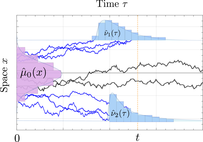
Figure 1: Matching spatio-temporal distributions starting from $\hat{\mu}_{0}$ (spatial) to $\hat{\nu}_{1}$ and $\hat{\nu}_{2}$ (temporal). Paths in blue are random walks that are absorbed over the time window $[1,t]$, while paths in black are walks that are not absorbed over it. The requirement is to find the most likely law $P^{\star}$ on all of these paths.

Thus, to recap, given the starting distribution $\hat{\mu}_{0}$ of random walkers $(X_{\tau})_{\tau\geq 0}$ on the graph $\mathcal{G}$, with support on ${\mathcal{V}_{\rm trs}}$, and spatio-temporal distributions $\hat{\nu}_{1},\ldots,\hat{\nu}_{m}$ with support on ${\mathcal{V}_{\rm abs}}\times\{1,\ldots,t\}$, signifying first-arrivals, the updated law $P^{\star}$ assigns accordant amounts of probability mass on sets of space-time indices and is closest to a given prior law. Figure 1 exemplifies the referred problem at hand as the Schrödinger Bridge Problem between $\hat{\mu}_{0}$ and $\hat{\nu}_{1},\ldots,\hat{\nu}_{m}$. Our control task amounts to specifying a suitable protocol for transition probabilities that allocates mass $\hat{\nu}_{j}$ at a selection $j\in{\mathcal{V}_{\rm abs}}$ of sites at arrival. This is done next.

The salient feature of our approach is that the prior, realized by a sequence of transition probabilities, provides a reference stochastic evolution on the graph. This prior may incorporate knowledge of the cost to traverse edges and serves as a baseline, with the only requirement that it has a Markovian structure. The (most likely) posterior, which we already know is Markov, will be obtained by adjusting the transition probabilities of the prior. This adjustment at each point in time represents the desired control action. Regulating the flow on the graph to meet first absorption time requirements over a finite window is of significant practical interest, and it is the problem at hand.

5.1 Problem Formulation

We express a prior law on paths in $\mathcal{V}^{t+1}$ as

$$Q(\mathbf{x})=\mu_{0}(x_{0})\Pi_{1}(x_{0},x_{1})\Pi_{2}(x_{1},x_{2})\ldots\Pi_{t}(x_{t},x_{t}),$$ (10)

where $\Pi_{\tau}$ denotes a transition kernel on $\mathcal{V}\times\mathcal{V}$. Thus, viewing $\Pi_{\tau}$ as a row-stochastic matrix indexed by time $\tau\in[1,t]\subset\mathbb{N}$, we write

$$\Pi_{\tau}=\begin{bmatrix}I&\mathbf{0}\\ B_{\tau}&A_{\tau}\end{bmatrix},$$ (11)

where $I,\mathbf{0}$ denote identity and the zero matrices, respectively. Therefore,

$$B_{\tau}(x,y)=\Pi_{\tau}(x,y),\ A_{\tau}(x,z)=\Pi_{\tau}(x,z),$$

for all $x,z\in{\mathcal{V}_{\rm trs}}$ and $y\in{\mathcal{V}_{\rm abs}}$. Once again, from Theorem 4.4, we know that the solution to Problem 4.3 is Markov. Hence, our aim now is to construct explicitly the optimal transition kernels $\{\Pi^{\star}_{\tau}\}_{\tau=1}^{t}$ realizing the most likely law $P^{\star}$ with $\hat{\mu}_{0}$ as the given initial distribution and $\hat{\nu}_{1},\ldots,\hat{\nu}_{m}$ as the given time-marginals at the absorption sites $j\in{\mathcal{V}_{\rm abs}}$. That is, our task is to search for the optimal $P^{\star}$ over laws of the form

$$P(\mathbf{x})=\hat{\mu}_{0}(x_{0})\hat{\Pi}_{1}(x_{0},x_{1})\hat{\Pi}_{2}(x_{1},x_{2})\ldots\hat{\Pi}_{t}{(x_{t-1},x_{t})},$$ (12)

with each $\hat{\Pi}_{\tau}$ row-stochastic of a similar form,

$$\hat{\Pi}_{\tau}=\begin{bmatrix}I&\mathbf{0}\\ \hat{B}_{\tau}&\hat{A}_{\tau}\end{bmatrix},$$ (13)

with

$$\hat{B}_{\tau}(x,y)=\hat{\Pi}_{\tau}(x,y),\ \hat{A}_{\tau}(x,z)=\hat{\Pi}_{\tau}(x,z),$$

for $x,z\in{\mathcal{V}_{\rm trs}}$ and $y\in{\mathcal{V}_{\rm abs}}$. The problem is set as follows.

Problem 5.1.

Consider a (prior) Markov law $Q$ on paths in $\mathcal{V}^{t+1}$ as in (10) over the time window $[0,t]$, together with a probability vector $\hat{\mu}_{0}$ with support on ${\mathcal{V}_{\rm trs}}\subset\mathcal{V}$, and non-negative (row) vectors $\{\hat{\nu}_{j}(\tau)\mid j\in{\mathcal{V}_{\rm abs}},\;\tau\in\{1,\ldots,t\}\}$, for first-arrival time distributions at nodes in ${\mathcal{V}_{\rm abs}}$, such that

$$\sum_{j=1}^{m}\sum_{\tau=1}^{t}\hat{\nu}_{j}(\tau)\leq 1.$$

Determine transition kernels $\{\Pi_{\tau}^{\star}\}_{\tau=1}^{t}$ for the (Markov) law

$$P^{\star}=\arg\min_{P}\mathbb{D}(P\|Q),$$ (14a)

with $$P$$ of the form (12) and subject to

$$\hat{\mu}_{0}(x_{0}) =\sum_{x_{1},\ldots,x_{t}\in\mathcal{V}}P(x_{0},x_{1},\ldots,x_{t}),$$ (14b)

$$\hat{\nu}_{j}(\tau) =\sum_{\mathbf{x}\in{\mathcal{X}_{x_{\tau}=j}}}P(\mathbf{x}),$$ (14c)

for any $j\in{\mathcal{V}_{\rm abs}}$, where

$${\mathcal{X}_{x_{\tau}=j}}:=\{\mathbf{x}=(x_{0},\ldots,x_{t})\mid x_{0},\ldots,x_{\tau-1}\neq j,x_{\tau}=j\}$$

is the set of paths that first arrive at $j$ at the time instant $\tau$. $\Box$

We proceed with technical propositions that help us build the solution. At first, we consider a one-step-in-time bridge problem to reconcile partially specified marginals (Section 5.2). This is followed by displaying the form of the optimal Markov kernels (13) building the optimizer $P^{\star}$ via a recursive argument on partially specified marginals (Section 5.3). We conclude with an explicit verification that the solution we provide is optimal (Section 5.4). The explicit construction of the Markov law provides an alternative independent argument that proves Theorem 4.4. The transition kernels of the optimal Markov protocol can be employed to steer random walkers to fulfill the prescribed space-time marginals ($\hat{\mu}_{0},\hat{\nu}_{1},\ldots,\hat{\nu}_{m}$), on average.

5.2 Building Space-Time Bridges I: Single-Stage Optimization with Partial Marginals

Consider an $n\times(m+\ell)$ transition probability matrix $\pi$, partitioned as

$$\pi=\begin{bmatrix}\mathcal{B}&\mathcal{A}\end{bmatrix},$$

with respect to two sets of states in its row span; thus, $\mathcal{B}$ and $\mathcal{A}$ have the same number of rows, whereas $m$ and $\ell$ represent the cardinality of two sets of states. The row-stochasticity,

$$\sum_{y=1}^{m+\ell}\pi(x,y)=1,$$

will be compactly expressed as

$$\pi\mathds{1}=\mathds{1},$$

where $\mathds{1}$ is a (column) vector of $1$’s of suitable size.

We remark that in subsequent sections, referring to our earlier notation, we will take

$$\mathcal{B}=[B_{1},\,A_{1}B_{2},\ldots,\,(A_{1}\cdots A_{t-1})B_{t}],$$

and $\mathcal{A}=(A_{1}\cdots A_{t})$. Then, it will hold that $\ell=n$, but here we let $\ell$ be arbitrary for generality. Incidentally, if the prior kernel is time-invariant, then $\mathcal{B}=[B,\,AB,\ldots,\,A^{t-1}B]$ and $\mathcal{A}=A^{t}$ are simpler and perhaps more familiar.

Consider now that we are given a marginal probability (column) vector $\hat{\mu}\in\mathbb{R}^{n}$, and another partially-specified marginal on the first $m$ states of the row span; that is, we are given a non-negative (column) vector $\hat{\nu}$ with $\sum_{y=1}^{m}\hat{\nu}(y)\leq 1$. Without loss of generality we may assume that

$$\hat{\mu}^{T}\mathcal{B}\neq\hat{\nu}^{T},$$

with ^T being vector transpose, and the task is to determine the transition probability matrix $\pi^{\star}$, partitioned similarly as

$$\pi^{\star}=\begin{bmatrix}\mathcal{B}^{\star}&\mathcal{A}^{\star}\end{bmatrix},$$

so that

$$\hat{\mu}^{T}\mathcal{B}^{\star}=\hat{\nu}^{T},$$

following Schrödinger’s dictum. Thus, we seek the solution to the following problem.

Problem 5.2.

Determine

$$\pi^{\star}=\scalebox{0.9}{\mbox{$\displaystyle{\rm arg}\min_{\hat{\pi}}\left\{\sum_{x,y}\hat{\mu}(x)\hat{\pi}(x,y)\log\frac{\hat{\pi}(x,y)}{\pi(x,y)}\mid\hat{\mu}^{T}\hat{\mathcal{B}}=\hat{\nu}^{T},\;\hat{\pi}\mathds{1}=\mathds{1}\right\}$}}$$

where $\hat{\pi}=\begin{bmatrix}\hat{\mathcal{B}}&\hat{\mathcal{A}}\end{bmatrix}\in\mathbb{R}^{n\times(m+\ell)}$. $\Box$

Remark 5.3.

Throughout, we tacitly assume feasibility when dealing with optimization problems. In the present context, reconciling marginals that are “partially specified on both ends” can also be treated similarly. However, for simplicity, we refrain from this additional layer of generality as it will not be needed in the sequel. $\square$

Assuming feasibility, we readily obtain the form of the minimizer by considering the Lagrangian

$$\mathcal{L}= \sum_{x=1}^{n}\hat{\mu}(x)\left[\sum_{y=1}^{m}\hat{\mathcal{B}}(x,y)\log\frac{\hat{\mathcal{B}}(x,y)}{\mathcal{B}(x,y)}+\sum_{y=1}^{\ell}\hat{\mathcal{A}}(x,y)\log\frac{\hat{\mathcal{A}}(x,y)}{\mathcal{A}(x,y)}\right]$$

$$+\sum_{x=1}^{n}\sum_{y=1}^{m}\lambda(y)\bigg{(}\hat{\mu}(x)\hat{\mathcal{B}}(x,y)-\hat{v}(y)\bigg{)}$$

$$+\sum_{x=1}^{n}d(x)\left(\sum_{y=1}^{m}\hat{\mathcal{B}}(x,y)+\sum_{y=1}^{\ell}\hat{\mathcal{A}}(x,y)-1\right),$$

with $\lambda\in\mathbb{R}^{m}$, $d\in\mathbb{R}^{n}$ being Lagrange multiplier vectors. Setting the partial derivatives with respect to the entries of $\hat{\mathcal{B}},\hat{\mathcal{A}}$ to zero, gives that the minimizer has the form

$$\mathcal{B}^{\star}(x,y) =\mathcal{B}(x,y)e^{{-\frac{1+d(x)}{\hat{\mu}(x)}}}e^{-\lambda(y)},$$

$$\mathcal{A}^{\star}(x,y) =\mathcal{A}(x,y)e^{{-\frac{1+d(x)}{\hat{\mu}(x)}}}.$$

Thus, the Lagrange multipliers effectively scale the two matrices $\mathcal{B}$ and $\mathcal{A}$, via left and right multiplication by diagonal matrices (“diagonal scaling”)

$$\mathbf{D}={\rm diag}(D_{x}),\mbox{ and }\mathbf{\Lambda}={\rm diag}(\Lambda_{y}),$$

with

$$D_{x}(x) :=e^{{-\frac{1+d(x)}{\hat{\mu}(x)}}},$$

$$D_{y}(y) :=e^{-\lambda(y)},$$

and where both $\mathcal{B},\mathcal{A}$ are multiplied on the left by $\mathbf{D}$ and only $\mathcal{B}$ on the right by $\mathbf{\Lambda}$, as stated next. Furthermore, these diagonal scalings are uniquely determined iteratively by a Sinkhorn-type algorithm.

Proposition 5.4.

The solution to Problem 5.2, assuming feasibility, is of the form

$$\mathcal{B}^{\star} =\mathbf{D}\mathcal{B}\mathbf{\Lambda},$$

$$\mathcal{A}^{\star} =\mathbf{D}\mathcal{A},$$

for diagonal matrices $\mathbf{D},\mathbf{\Lambda}$. If $D,\Lambda$ denote the (column) vectors of the respective diagonal entries of $\mathbf{D},\mathbf{\Lambda}$, these vectors can be obtained as the limits to the following Sinkhorn iteration (with $\Lambda^{(k)},D^{(k)},\hat{\mu},\hat{\nu}$ being column vectors):

$$\Lambda^{(k)} \mapsto D^{(k)}=\hat{\mu}\oslash(\mathcal{B}\Lambda^{(k)}+\mathcal{A}\mathds{1}),$$ (15a)

$$D^{(k)} \mapsto \Lambda^{(k+1)}=\hat{\nu}\oslash\mathcal{B}^{T}D^{(k)},$$ (15b)

carried out for $k=1,2,\ldots$ and initialized by taking $\Lambda^{(1)}=\mathds{1}$, where $\oslash$ denotes entry-wise division of column vectors.

Proof 5.5.

The proof follows standard arguments, as in [26], [27, Section 4.2], by noting that each step in (15) is either contractive or isometric in the Hilbert metric.

5.3 Building Space-Time Bridges II: Multi-Stage Optimization with Partial Marginals

We now consider the Markov model (10), (11) and write the probability kernel of the corresponding random walk $(X_{\tau})_{0\leq\tau\leq t}$, transitioning from ${\mathcal{V}_{\rm abs}}$ to

$$\underbrace{{\mathcal{V}_{\rm abs}}\times{\mathcal{V}_{\rm abs}}\times\ldots\times{\mathcal{V}_{\rm abs}}}_{\mbox{stopped process over}\ [1,t]}\times{\mathcal{V}_{\rm trs}}$$

via a “telescopic” expansion of successive transitions

$$\varPi=\begin{bmatrix}B_{1}&A_{1}B_{2}&\ldots&(A_{1}\cdots A_{t-1})B_{t}&(A_{1}\cdots A_{t})\end{bmatrix}.$$

Thus, e.g., the $(x,y)$-entry of $A_{1}B_{2}$ quantifies the probability that a random walker at $X_{0}=x$ first arrives at the absorbing node $y$ at $\tau=2$, and so on. Then, $(A_{1}\cdots A_{t})$ is the transition probability matrix into the transitory states for walkers that have avoided being absorbed over the window $[1,t]$.

We now consider as data the marginal distribution $\hat{\mu}_{0}$ on ${\mathcal{V}_{\rm trs}}$, for the random walk at time $\tau=0$, and the time-space marginal distribution

$$\hat{\nu}^{T}:=[\underbrace{\hat{\nu}_{1}(1),\ldots,\hat{\nu}_{m}(1)}_{\mbox{stopped at $\tau=1$}},\underbrace{\hat{\nu}_{1}(2)\ldots,\hat{\nu}_{m}(2)}_{\mbox{stopped at $\tau=2$}},\ldots,\hat{\nu}_{m}(t)],$$

that encapsulates our complete information on first-time arrivals at the absorption nodes in ${\mathcal{V}_{\rm abs}}$ at different times, from $\tau=1$ to $\tau=t$. We partition $\Pi$ into two submatrices,

$$\varPi=[\underbrace{B_{1},\;A_{1}B_{2},\ldots(A_{1}\cdots A_{t-1})B_{t}}_{\mathcal{B}},\;\underbrace{(A_{1}\cdots A_{t})}_{\mathcal{A}}],$$

and apply Proposition 5.4 directly. We deduce that there exists a unique pair of diagonal scalings, $\mathbf{D}_{0}$ on the left and

$$\mathbf{\Lambda}=\rm{diag}(\mathbf{\Lambda}_{1},\ldots,\mathbf{\Lambda}_{t})$$

on the right, so that the solution to Problem 5.2 is of the form

$$\varPi^{\star}= \mathbf{D}_{0}\varPi\begin{bmatrix}\mathbf{\Lambda}_{1}&0&\ldots&0&0\\ 0&\mathbf{\Lambda}_{2}&\ldots&0&0\\ \vdots&&&&\\ 0&0&\ldots&\mathbf{\Lambda}_{t}&0\\ 0&0&\ldots&0&I\end{bmatrix}.$$ (16)

Note that in (16) $\mathbf{\Lambda}$ is further partitioned in a block diagonal structure, with the blocks being themselves diagonal, conformally with the finer structure of $\mathcal{B}$. Thus, we write $\Pi^{\star}$ as

$$\begin{array}[]{cccccc}[\mathbf{D}_{0}B_{1}\mathbf{\Lambda}_{1},&\mathbf{D}_{0}A_{1}\overbrace{\begin{bmatrix}B_{2}\mathbf{\Lambda}_{2},&A_{2}B_{3}\mathbf{\Lambda}_{3},&\ldots&(A_{2}\cdots A_{t})\end{bmatrix}}^{{\mathcal{C}}_{2:t+1}}].\end{array}$$

Our goal now is to show that $\Pi^{\star}$ arises as a transition probability of a Markov law. For this reason, in the above listing of the block entries of $\Pi^{\star}$ we see a nested structure, and define ${\mathcal{C}}_{2:t+1}$ accordingly, as in the displayed equation above. We will return to exploring the structure of ${\mathcal{C}}_{2:t+1}$ shortly.

The scalings in Proposition 5.4 ensure that the solution is row-stochastic, i.e., $\varPi^{\star}\mathds{1}=\mathds{1}$. Note that the notation ${\mathcal{C}}_{2:t+1}$ subscribes the listing of the block entries, where the last one corresponds to transitioning to ${\mathcal{V}_{\rm trs}}$ at the end of the $t^{th}$ time-step. Note that ${\mathcal{C}}_{2:t+1}$ may not be row stochastic. Next we determine diagonal scaling of ${\mathcal{C}}_{2:t+1}$ to ensure it becomes row stochastic.

To this end, let ${\mathcal{C}}_{2:t+1}\mathds{1}=d_{1}\neq\mathds{1}$, in general. Then, let $\mathbf{D}_{1}={\rm diag}(d_{1})^{-1}$ and rewrite $\Pi^{\star}$ as

$$\begin{array}[]{cccccc}[\mathbf{D}_{0}B_{1}\mathbf{\Lambda}_{1},&\mathbf{D}_{0}A_{1}\mathbf{D}_{1}^{-1}\overbrace{\begin{bmatrix}\mathbf{D}_{1}B_{2}\mathbf{\Lambda}_{2},&\mathbf{D}_{1}A_{2}B_{3}\mathbf{\Lambda}_{3},&\ldots&\end{bmatrix}}^{\mathbf{D}_{1}{\mathcal{C}}_{2:t+1}}].\end{array}$$

Now, since $\mathbf{D}_{1}{\mathcal{C}}_{2:t+1}\mathds{1}=\mathds{1}$ is row-stochastic, so is

$$[\mathbf{D}_{0}B_{1}\mathbf{\Lambda}_{1},\;\mathbf{D}_{0}A_{1}\mathbf{D}_{1}^{-1}].$$

Recursively and in the same way, by considering this telescopic expansion, we construct the sequence of diagonal scalings $\mathbf{D}_{1},\mathbf{D}_{2},\ldots,$ via

$$\mathbf{D}_{\tau}={\rm diag}(d_{\tau})^{-1}\mbox{ for }d_{\tau}={\mathcal{C}}_{\tau+1:t+1}\mathds{1},$$

so that

$$\varPi^{\star}=\begin{bmatrix}B_{1}^{\star}&A_{1}^{\star}B_{2}^{\star}&\ldots&(A_{1}^{\star}\cdots A_{t-1}^{\star})B_{t}^{\star}&(A_{1}^{\star}\cdots A_{t}^{\star})\end{bmatrix},$$

with

$$\begin{split}B^{\star}_{\tau}&=\mathbf{D}_{\tau-1}B_{\tau}\mathbf{\Lambda}_{\tau},\\ A^{\star}_{\tau}&=\mathbf{D}_{\tau-1}A_{\tau}\mathbf{D}_{\tau}^{-1},\end{split}$$ (17)

for $\tau\in\{1,\ldots,t\}$.

Equations (17) provide the parameters of the sought solution to Problem 5.1. We first recap that these provide an admissible Markov law which is consistent with the marginals, and in the next section, we argue that it, in fact, minimizes the likelihood function (14a).

Proposition 5.6.

The Markov law (12) with transition kernel (13) and $B_{\tau}^{\star},A_{\tau}^{\star}$ as in (17) is consistent with the given marginals $\hat{\mu},\hat{\nu}_{1}\ldots,\hat{\nu}_{t}$ for the distribution at $t=0$, and absorption masses prescribed by $\hat{\nu}_{\tau}$.

Proof 5.7.

The proposition has been established by the proceeding arguments in this section. Indeed, $\Pi^{\star}$ is of the required form

$$[B^{\star}_{1},\,A_{1}^{\star}B_{2}^{\star},\ldots],$$

with $[B_{\tau}^{\star},\,A_{\tau}^{\star}]$ row stochastic, and

$$\hat{\mu}^{T}[B_{1}^{\star},\,\ldots(A_{1}^{\star}\cdots A_{t-1}^{\star})B_{t}^{\star}]=\hat{\nu}^{T},$$

as required.

5.4 Building Space-Time Bridges III: Optimality of the Law

We are now in a position to establish our central result, that the Markov law identified in Proposition 5.6 is in fact the optimal solution claimed in Theorem 4.4. It is important to note that so far we have only established that $\Pi^{\star}$ minimizes the relative entropy functional in Problem 5.2; this optimization revealed the structure of the solution. We still need to consider how the law distributes probability mass on individual paths, and that it is optimal in that it minimizes the relative entropy (6a) on paths as well. This is a consequence of the diagonal structure of scalings.

Indeed, the analysis leading to Proposition 5.6 does not take into account how the law weighs in different paths from start to finish. The key to establishing our result is to observe first that the prior law $Q$ and the posterior $P^{\star}$ “share the same bridges,” i.e., under either law the probability of transitioning from $x_{0}$ to $x_{\tau}\in{\mathcal{V}_{\rm abs}}$ (and $x_{\tau-1}\notin{\mathcal{V}_{\rm abs}}$) along any particular path $(x_{0},x_{1},...,x_{\tau})$ is a function of the path and it is the same for either law. Likewise, the probability of transitioning from $x_{0}$ to $x_{t}\in{\mathcal{V}_{\rm trs}}$ is also a function of the path but again identical for both laws. This is shown next.

Proposition 5.8.

Consider Markov laws (10) and (12), with transition kernels $\Pi_{\tau}$ and $\hat{\Pi}_{\tau}$ as in (11) and (13), respectively. If $\hat{\Pi}=\Pi^{\star}$ as in (17), with matrices $\mathbf{D},\mathbf{\Lambda}$ being diagonal, then the probability mass on any path $\mathbf{x}=(x_{0},\ldots,x_{\tau})$, with $x_{\tau}\in{\mathcal{V}_{\rm abs}}$ and $x_{\tau^{\prime}}\notin{\mathcal{V}_{\rm abs}}$ for $\tau^{\prime}<\tau$, is the same for both laws. The same is true for any path $\mathbf{x}$ when $\tau=t$ and $x_{t}\in{\mathcal{V}_{\rm trs}}$.

Proof 5.9.

If we specify the starting and ending nodes of a path, in general,

$$Q(\mathbf{x}\mid x_{0},x_{\tau})=\Pi_{1}(x_{0},x_{1})\cdots\Pi_{\tau}(x_{\tau-1},x_{\tau})/Z$$ (18)

where

$$Z=\sum_{x_{1},\ldots,x_{\tau-1}\in{\mathcal{V}_{\rm trs}}}\Pi_{1}(x_{0},x_{1})\cdots\Pi_{\tau}(x_{\tau-1},x_{\tau})$$

is a normalizing factor (though its exact value is unimportant). Bringing in the form of the kernels in (11), in the case where $x_{\tau}\in{\mathcal{V}_{\rm abs}}$ while $x_{\tau^{\prime}}\notin{\mathcal{V}_{\rm abs}}$ for $\tau^{\prime}<\tau$, we have that the product $\Pi_{1}(x_{0},x_{1})\cdots\Pi_{\tau}(x_{\tau-1},x_{\tau})$ in (18) is proportional to

$$A_{1}(x_{0},x_{1})\cdots A_{\tau-1}(x_{\tau-2},x_{\tau-1})B_{\tau}(x_{\tau-1},x_{\tau}).$$

Similarly, we obtain that $P^{\star}(\mathbf{x}\mid x_{0},x_{\tau})$ is proportional to

$$D_{0}(x_{0})A_{1}(x_{0},x_{1})\!\cdots\!A_{\tau-1}(x_{\tau-2},x_{\tau-1})B_{\tau}(x_{\tau-1},x_{\tau})\Lambda_{\tau}(x_{\tau}).$$

Since $x_{0}$ and $x_{\tau}$ are fixed, $D_{0}(x_{0})\Lambda_{\tau}(x_{\tau})$ is independent of $(x_{1},\ldots,x_{\tau-1})$. Thus, the probability of traversing the segment $(x_{1},\ldots,x_{\tau-1})$, starting from $x_{0}$ and reaching ${\mathcal{V}_{\rm abs}}$ at $\tau$ and at a particular $x_{\tau}$ is identical for the two laws.

Similarly, if we pin the bridge to values $x_{0}\in{\mathcal{V}_{\rm trs}}$ and $x_{t}\in{\mathcal{V}_{\rm trs}}$ at the two endpoints, the probability mass on any particular path, while also a function of the path, is once again the same for the two laws. The verification is identical.

We close the section by stating and proving one of our main results.

Theorem 5.10.

The Markov law (12) with transition kernel (13) and $\hat{B}_{\tau}=B_{\tau}^{\star},\hat{A}_{\tau}=A_{\tau}^{\star}$ as in (17), is the unique solution $P^{\star}$ to Problem 5.1.

Proof 5.11.

Recall that the construction of $B_{\tau}^{\star},A_{\tau}^{\star}$ involves diagonal scalings selected so as to satisfy the given marginals $\hat{\mu},\hat{\nu}_{1}\ldots,\hat{\nu}_{m}$ for the distribution at $t=0$, and first arrival probabilities $\hat{\nu}_{y}$ at the nodes $y\in{\mathcal{V}_{\rm abs}}$. To establish the optimality of the relative entropy functional, the basic idea is to disintegrate the probability mass on paths into a product of two terms. In this, one term represents the joint between marginals at end-points $x_{0}$ and $x_{\tau}$ (with $x_{0}\in{\mathcal{V}_{\rm trs}}$ and $(\tau,x_{\tau})$ in $\{1,\ldots t\}\times{\mathcal{V}_{\rm abs}}$ or in $\{t\}\times{\mathcal{V}_{\rm trs}}$) and the other represents the probability mass on the in-between choice of path. The relative entropy between the prior $Q$ and the posterior $P$, upon substitution, decomposes into summands that correspond to the respective terms of the disintegrated measure. One summand has already been optimized in our selection of $P^{\star}$ whereas the other vanishes, since $Q$ and $P^{\star}$ share the same mass on their pinned bridges (Proposition 5.8). We now explain this in detail. To this end, we partition the set of possible paths into a union of disjoint sets

$$\mathcal{V}_{\rm trs}^{t+1}\mbox{ and }\left\{\mathcal{X}_{x_{\tau}=j}\mid\tau\in\{1,\ldots,\,t\},j\in{\mathcal{V}_{\rm abs}}\right\}.$$

These are $1+tm$ sets, since $|{\mathcal{V}_{\rm abs}}|=m$. For notational convenience we enumerate these sets letting $\mathcal{S}_{0}=\mathcal{V}_{\rm trs}^{t+1}$ and $\mathcal{S}_{k}=\mathcal{X}_{x_{\tau}=j}$, for $k=1,\ldots,\,tm$, listing the sets lexicographically, numbering sequentially states in ${\mathcal{V}_{\rm abs}}$ in subsequent time instances. Then, consider the relative entropy $\mathbb{D}(P^{\star}\|Q)$ and observe that

$$\mathbb{D}(P^{\star}\|Q)=\sum_{k=0}^{tm}P^{\star}(\mathcal{S}_{k})\log\frac{P^{\star}(\mathcal{S}_{k})}{Q(\mathcal{S}_{k})}.$$

Accordingly, we disintegrate the measures $P^{\star}$ and $Q$, and write

$$Q(\mathbf{x})=Q(\mathbf{x}|x_{0},x_{\tau})Q(x_{0},x_{\tau})$$

where $Q(x_{0},x_{\tau})$ is the end-point marginal. The same applies to $P^{\star}$. By Proposition 5.8, $Q(\mathbf{x}|x_{0},x_{\tau})=P^{\star}(\mathbf{x}|x_{0},x_{\tau})$ for all $\mathbf{x}$’s on each of those sets. Therefore, $\mathbb{D}(P^{\star}\|Q)$ equals

$$\sum_{k=0}^{tm}\sum_{\mathbf{x}\in\mathcal{S}_{k}}P^{\star}(x_{0},x_{\tau})P^{\star}(\mathbf{x}|x_{0},x_{\tau})\log\frac{P^{\star}(x_{0},x_{\tau})}{Q(x_{0},x_{\tau})}.$$

Evidently, $P^{\star}(\mathbf{x}|x_{0},x_{\tau})$, when summing over $x_{1},\ldots,x_{\tau-1}$ is $1$, and therefore the relative entropy between the two laws is dictated by the restriction of the laws on the coupling between their respective marginal distributions, namely,

$$\mathbb{D}(P^{\star}\|Q)=\sum_{k=0}^{tm}\sum_{\mathbf{x}\in\mathcal{S}_{k}}P^{\star}(x_{0},x_{\tau})\log\frac{P^{\star}(x_{0},x_{\tau})}{Q(x_{0},x_{\tau})}.$$

Disintegrating one more time, we have that $Q(x_{0},x_{\tau})=\mu(x_{0})\pi(x_{0},x_{\tau})$ where $\pi(x_{0},x_{\tau})=Q(x_{\tau}|x_{0})$ is the conditional, and similarly, $P^{\star}(x_{0},x_{\tau})=\hat{\mu}(x_{0})\pi^{\star}(x_{0},x_{\tau})$. Then,

$$\mathbb{D}(P^{\star}\|Q)= \sum_{k=0}^{tm}\sum_{\mathbf{x}\in\mathcal{S}_{k}}\hat{\mu}(x_{0})\pi^{\star}(x_{0},x_{\tau})\left(\log\frac{\hat{\mu}(x_{0})}{\mu(x_{0})}\right)$$

$$+\sum_{k=0}^{tm}\sum_{\mathbf{x}\in\mathcal{S}_{k}}\hat{\mu}(x_{0})\pi^{\star}(x_{0},x_{\tau})\left(\log\frac{\pi^{\star}(x_{0},x_{\tau})}{\pi(x_{0},x_{\tau})}\right).$$

Since $\pi^{\star}(x_{0},x_{\tau})$, when summed over all admissible $x_{\tau}$, is $1$,

$$\mathbb{D}(P^{\star}\|Q)= \sum_{x_{0}\in{\mathcal{V}_{\rm trs}}}\hat{\mu}(x_{0})\left(\log\frac{\hat{\mu}(x_{0})}{\mu(x_{0})}\right)$$

$$+\sum_{k=0}^{tm}\sum_{\mathbf{x}\in\mathcal{S}_{k}}\hat{\mu}(x_{0})\pi^{\star}(x_{0},x_{\tau})\left(\log\frac{\pi^{\star}(x_{0},x_{\tau})}{\pi(x_{0},x_{\tau})}\right).$$

The first term is independent of our choice of $P^{\star}$ whereas the second is optimal by Proposition 5.4, attesting optimality in the context of Problem 5.2 that sought coupling transition probabilities to match space-time marginals. This completes the proof.

6 Regularized transport on Graphs

The variational formalism where, in the spirit of Schrödinger we minimize a relative entropy functional, is fairly flexible and can incorporate the cost of transportation into our model. Specifically, suppose that we would like to select a Markovian policy for guiding walkers on a graph so as to minimize on average a transportation cost in their journey between their original starting distribution to their respective destinations. As in the setting of the earlier theory, their distribution at the end of their journey can be both in space and time, reaching with specified arrival distributions absorbing states.

Now assume that the cost of traversing an edge $(x_{\tau},x_{\tau+1})$ at time $\tau$ is known and quantified by a function $U_{\tau}(x_{\tau},x_{\tau+1})$. Evidently, the cost of transporting along $\mathbf{x}=(x_{0},\ldots,x_{t})$ is

$$U(\mathbf{x}):=\sum_{\tau\in\{0,\ldots,t-1\}}U_{\tau}(x_{\tau},x_{\tau+1}),$$

and the cumulative cost of transporting a distribution of random walkers with law $P$ over a window in time $[0,t]$ is

$$\mathbb{J}(P) =\sum_{\mathbf{x}}P(\mathbf{x})U(\mathbf{x}),$$

where the summation runs over paths that satisfy specifications. As explained in [15, 5], there are often practical advantages in modifying the cost functional of our control problem by adding a regularizing entropic term to the control cost, e.g., to minimize

$$\mathbb{J}(P)+\beta^{-1}\sum_{\mathbf{x}}P(\mathbf{x})\log P(\mathbf{x}).$$

The constant $\beta^{-1}$ is thought of as “temperature” and helps match the units to those of $U$. From another angle, increased “temperature” promotes randomness in selecting alternative paths and thereby trades off cost for robustness [15].

More generally we may choose to penalize the entropic (relative entropy) distance of the sought solution $P$ from a given prior law $Q$. As before $Q$ may be available as a point of reference. Thus, we may adopt a “free energy” functional,

$$\mathbb{F}(P\|Q):=\mathbb{J}(P)+\beta^{-1}\mathbb{D}(P\|Q),$$

to replace $\mathbb{J}$ as our optimization functional, and seek solutions to the following problem.

Problem 6.1.

Consider a (prior) Markov law $Q$ on paths in $\mathcal{V}^{t+1}$ as in (10) over the time window $[0,t]$, together with a probability vector $\hat{\mu}_{0}$ with support on ${\mathcal{V}_{\rm trs}}\subset\mathcal{V}$, and non-negative (row) vectors $\{\hat{\nu}_{j}(\tau)\mid j\in{\mathcal{V}_{\rm abs}},\;\tau\in\{1,\ldots,t\}\}$, for first-arrival time distributions at nodes in ${\mathcal{V}_{\rm abs}}$, such that

$$\sum_{j=1}^{m}\sum_{\tau=1}^{t}\hat{\nu}_{j}(\tau)\leq 1.$$

Determine transition kernels $\{\Pi_{\tau}^{\star}\}_{\tau=1}^{t}$ for the law

$$P^{\star}=\arg\min_{P}\mathbb{F}(P\|Q),$$ (19a)

subject to

$$\hat{\mu}_{0}(x_{0}) =\sum_{x_{1},\ldots,x_{t}\in\mathcal{V}}P(x_{0},x_{1},\ldots,x_{t}),$$ (19b)

$$\hat{\nu}_{j}(\tau) =\sum_{\mathbf{x}\in{\mathcal{X}_{x_{\tau}=j}}}P(\mathbf{x}),$$ (19c)

for any $j\in{\mathcal{V}_{\rm abs}}$. $\Box$

Observing that

$$\mathbb{J}(P)=-\beta^{-1}\sum_{\mathbf{x}}P(\mathbf{x})\log e^{-\beta U(\mathbf{x})},$$

we can write that

$$\mathbb{F}(P\|Q)=\mathbb{D}(P\|Qe^{-\beta U}).$$

This is identical in form to the relative entropy, albeit, the second term $Qe^{-\beta U}$ that combines cost and prior is a positive measure that may not be normalized (hence, not necessarily a probability measure). Yet, all the steps in our previous analysis carry through and a law $P$ to optimize this mix of “cost” $+$ “distance from the nominal $Q$,” can be similarly obtained. The new “prior” $Qe^{-\beta U}$ inherits the Markovian factor structure from $Q$, since $e^{-\beta U}$ factors similarly as

$$e^{-\beta U}=f^{\rm cost}_{1}(x_{0},x_{1})\ldots f^{\rm cost}_{t}(x_{t-1},x_{t})$$

for

$$f^{\rm cost}_{\tau}(x_{\tau-1},x_{\tau})=e^{-\beta U_{\tau}(x_{\tau-1},x_{\tau})}.$$

Therefore, the posterior $P^{\star}$ that is obtained by minimizing $\mathbb{F}(P\|Q)$ subject to constraints on spatio-temporal marginals as before is also Markovian. We summarize as follows.

Theorem 6.2.

Assuming that Problem 6.1 is feasible, the solution $P^{\star}$ is unique and it is Markov.

Remark 6.3.

The construction of solutions to Problem 6.1 proceeds in precisely the same way as in the earlier sections where the prior is normalized. Moreover, if $P^{\star}_{\beta}$ denotes the solution as a function of $\beta$, taking $\beta^{-1}\to 0$ recovers the minimizing solution for $\mathbb{J}$. Entropic regularization, besides its practical significance, is often used in computation tools since minimizing $\mathbb{F}$ is more efficient than minimizing $\mathbb{J}$, and thus, standard practice in the recent literature of optimal mass transport and machine learning [28, 27]. $\Box$

7 Examples

Below we first return to our motivating example of reconciling wins and losses in a martingale game, where unlikely time marginals may reveal a foul play. Next, we discuss a second academic example, to schedule probabilistic flow in a traffic network so as to regulate the flow rate across critical points. The setting is framed as transportation through bridges that link a city to its downtown. Passing through either bridge is a stopping criterion. We then postulate that one of the bridges closes during peak traffic hours, and seek to redirect traffic with a Markov policy so that we abide by a prescribed time marginal for the traffic going across to meet, e.g., capacity constraints.

7.1 De Moivre’s Martingale

We now reexamine the betting game in Section 2, abstracted via the graph in Figure 2. Consider that the players start the game with $1$ to $4$ tokens. Each state is represented as a node. In addition, node $0$ represents ruin while node $5$ represents the cap on profit that triggers exit from the game. Thus, nodes $0$ and $5$ are absorbing. Assume that the wealth of the players is distributed uniformly over the nodes $\{1,2,3,4\}$ at the start of the game. We let the prior law be that of a fair game, with equal probabilities of winning and losing. The prior transition probabilities are shown in Figure 2.

Figure 2: Network Topology

We assume that we observe three consecutive rounds. The portion of players exiting the game due to ruin or success is recorded, giving time marginals

$$\hat{\nu}^{\rm ruin}=\begin{bmatrix}1/8&\leavevmode\resizebox{15.00005pt}{7.5pt}{{1/5}}&1/16\end{bmatrix},\;\hat{\nu}^{\rm win}=\begin{bmatrix}1/8&1/16&1/16\end{bmatrix}.$$

While the fair game should result in $\hat{\nu}^{\rm ruin}=\hat{\nu}^{\rm win}$, we notice an unexpectedly large percentage of players exiting in the second round due to ruin. We seek to pinpoint possible cheating that could explain the marginals. To this end, we determine the most likely transition kernels $\{\Pi^{\star}_{\tau}\}_{\tau=1}^{3}$, in the format (13). Applying (17), we obtain

$$B^{\star}_{1} =\begin{bmatrix}\phantom{0}0.5\phantom{0}&0\\ 0&0\\ 0&0\\ 0&\phantom{0}0.5\phantom{0}\end{bmatrix},A^{\star}_{1}=\begin{bmatrix}0&\phantom{0}0.5\phantom{0}&0&0\\ \leavevmode\resizebox{18.22229pt}{5.15555pt}{{0.858}}&0&\leavevmode\resizebox{18.22229pt}{5.15555pt}{{0.142}}&0\\ 0&\phantom{0}0.5\phantom{0}&0&\phantom{0}0.5\phantom{0}\\ 0&0&\phantom{0}0.5\phantom{0}&0\\ \end{bmatrix},$$

$$B^{\star}_{2} =\begin{bmatrix}\leavevmode\resizebox{18.22229pt}{5.15555pt}{{0.933}}&0\\ 0&0\\ 0&0\\ 0&\phantom{0}0.5\phantom{0}\hskip 1.0pt\end{bmatrix},A^{\star}_{2}=\begin{bmatrix}0&\leavevmode\resizebox{18.22229pt}{5.15555pt}{{0.067}}&0&0\\ \phantom{0}0.5\phantom{0}\hskip 2.0pt&0&\phantom{0}0.5\phantom{0}&0\\ 0&\leavevmode\resizebox{18.22229pt}{5.15555pt}{{0.407}}&0&\leavevmode\resizebox{18.22229pt}{5.15555pt}{{0.593}}\\ 0&0&\phantom{0}0.5\phantom{0}&0\\ \end{bmatrix},$$

$$B^{\star}_{3} =\begin{bmatrix}\phantom{0}0.5\phantom{0}&0\\ 0&0\\ 0&0\\ 0&\leavevmode\resizebox{18.22229pt}{5.15555pt}{{0.657}}\end{bmatrix},A^{\star}_{3}=\begin{bmatrix}0&\phantom{0}0.5\phantom{0}&0&0\\ \phantom{0}0.5\phantom{0}&0&\phantom{0}0.5\phantom{0}&0\\ 0&\phantom{0}0.5\phantom{0}&0&\phantom{0}0.5\phantom{0}\\ 0&0&\leavevmode\resizebox{18.22229pt}{5.15555pt}{{0.343}}&0\\ \end{bmatrix},$$

that make up the desired transition kernels. The result suggests that the game may have been staged, in that with high probability ($80\%$ chance), players starting with two tokens will reach ruin in the second round. This shows up in the values of elements $A_{1}^{\star}(2,1)$ and $B_{2}^{\star}(1,0)$. In the third round, the chances of winning may have been tampered with again, so that the higher betters are more likely to win. This could be intentionally arranged to make the game look fair in the third round.

7.2 Traffic flow regulation

The graph in Fig. 3 abstracts traffic flow in a city, where nodes $3$ through $7$ represent neighborhoods while nodes $1$ and $2$ represent two bridges that connect the city to its downtown. We consider traffic flow during early rush hours and assume that the overwhelming majority of passengers cross either of the two bridges in one direction, towards the downtown, during the time window at hand. Thereby, we treat the bridges as absorption nodes and an eventual destination for all traffic.

With a plan to repair one of the bridges, the city hall aims to redirect traffic for the three hours of scheduled maintenance. During this time traffic must not exceed the capacity of the operating bridge to avoid traffic jams. We model this problem on a network with two absorbing states ${\mathcal{V}_{\rm abs}}=\{1,2\}$, with node $1$ being the bridge to be mended and $2$ being the one remaining operational. Traffic flow rates between nodes are seen as transition probabilities. Typical flow rates that serve to define the prior are shown in Figure 3. During times $\tau\in\{3,4,5\}$ of maintenance, a possible policy is to adjust the prior kernel redirecting towards the bridge that remains open, completing the prior by taking,

$$\Pi_{3}=\Pi_{4}=\Pi_{5}=\left[\begin{array}[]{c|c}\begin{matrix}1&0\\ 0&1\\ \end{matrix}&\begin{matrix}0\phantom{0}&&\cdots&&\phantom{0}0\\ 0\phantom{0}&&\cdots&&\phantom{0}0\end{matrix}\\ \hline\cr&\\[-10.0pt] \begin{matrix}0&0\\ 0&0\\ 0&0\\ 0&\frac{1}{2}\\[1.5pt] 0&\frac{1}{2}\end{matrix}&\begin{matrix}\frac{1}{3}&0&\frac{2}{3}&0&0\\ 0&\frac{1}{3}&0&0&\frac{2}{3}\\ 0&0&0&1&0\\[1.5pt] 0&0&\frac{1}{4}&0&\frac{1}{4}\\[1.5pt] 0&0&0&\frac{1}{2}&0\end{matrix}\end{array}\right].$$

Let the initial density on nodes be

$$\hat{\mu}=\begin{bmatrix}0.4&0.4&0.05&0.1&0.05\end{bmatrix}^{T}.$$

Figure 3: Cartoon Representation of A City Neighborhood with Normal Operation of The City Bridges

With both bridges open, the density at the bridges at all times remains $\leq 0.158$, but with the closing of one and the above prior, these become

$$\nu_{1} =\begin{bmatrix}0.05&0.158&0&0&0&0\end{bmatrix}$$

$$\nu_{2} =\begin{bmatrix}0.05&0.158&\leavevmode\resizebox{22.77785pt}{6.44444pt}{{0.197}}&0.127&0.101\end{bmatrix}.$$

We seek to adjust flow rates so as not to exceed capacity, say this being $0.17$, and thereby target obtaining time marginals

$$\hat{\nu}_{1} =\begin{bmatrix}0.05&0.158&0&0&0&0\end{bmatrix},$$

$$\hat{\nu}_{2} =\begin{bmatrix}0.05&0.158&0.142&0.142&0.142\end{bmatrix}.$$

Indeed, this is achieved by solving Problem 5.1 to obtain the respective optimal kernel via (17), giving,

$$D_{0}=\begin{bmatrix}0.975\\ 1.034\\ 1.008\\ 1.024\\ 1.008\end{bmatrix} ,\begin{bmatrix}\Lambda_{1}^{T}\\ \Lambda_{2}^{T}\\ \Lambda_{3}^{T}\\ \Lambda_{4}^{T}\\ \Lambda_{5}^{T}\end{bmatrix}=\begin{bmatrix}0.984&0.984\\ 1.019&0.97\\ 0&0.711\\ 0&1.108\\ 0&1.4\end{bmatrix},d_{1}=\begin{bmatrix}1.114\\ 0.987\\ 0.981\\ 1\\ 0.957\end{bmatrix},$$

$$d_{2}=\begin{bmatrix}1.133\\ 1.147\\ 1.104\\ 0.944\\ 0.908\end{bmatrix} ,d_{3}=\begin{bmatrix}1\\ 1.133\\ 1.2\\ 1.104\\ 1.154\end{bmatrix},d_{4}=\begin{bmatrix}1\\ 1\\ 1\\ 1.2\\ 1.2\\ \end{bmatrix},d_{5}=\begin{bmatrix}1\\ \vdots\\ 1\end{bmatrix}.$$

8 Concluding remarks

It is natural to consider analogous problems in continuous time and space, where a process is stopped when specific targets are reached and stopping criteria are met. Such problems are of evident practical significance. The present work shows that in discrete time and space, such problems can be treated within the theory of Schrödinger bridges. It is envisioned that the possibility to meet spatio-temporal distributional objectives, and with such specifications in place to solve optimization problems, will open a new phase in the developing topic of uncertainty control, see [16, 29, 30, 31, 32, 33, 34, 35].

References

• [1] E. Schrödinger, “Über die Umkehrung der Naturgesetze,” Sitzungsberichte der Preuss Akad. Wissen. Phys. Math. Klasse, Sonderausgabe, vol. IX, pp. 144–153, 1931.
• [2] E. Schrödinger, “Sur la théorie relativiste de l’électron et l’interprétation de la mécanique quantique,” in Annales de l’institut Henri Poincaré, vol. 2(4), pp. 269–310, Presses universitaires de France, 1932.
• [3] H. Cramér, “Sur un nouveau théoreme-limite de la théorie des probabilités,” Actual. Sci. Ind., vol. 736, pp. 5–23, 1938.
• [4] I. N. Sanov, On the probability of large deviations of random variables. United States Air Force, Office of Scientific Research, 1958.
• [5] Y. Chen, T. T. Georgiou, and M. Pavon, “Stochastic control liaisons: Richard Sinkhorn meets Gaspard Monge on a Schrödinger bridge,” Siam Review, vol. 63, no. 2, pp. 249–313, 2021.
• [6] B. Jamison, “Reciprocal processes,” Z. Wahrscheinlichkeitstheorie verw. Gebiete, vol. 30, pp. 65–86, 1974.
• [7] B. Jamison, “The Markov processes of Schrödinger,” Zeitschrift für Wahrscheinlichkeitstheorie und Verwandte Gebiete, vol. 32, no. 4, pp. 323–331, 1975.
• [8] H. Föllmer, “Random fields and diffusion processes,” Ecole d’Ete de Probabilites de Saint-Flour XV-XVII, 1985-87, 1988.
• [9] H. Föllmer and S. Orey, “Large deviations for the empirical field of a Gibbs measure,” The Annals of Probability, pp. 961–977, 1988.
• [10] I. Csiszár, “The method of Types,” IEEE Transactions on Information Theory, vol. 44, no. 6, pp. 2505–2523, 1998.
• [11] P. Dai Pra, “A stochastic control approach to reciprocal diffusion processes,” Applied Mathematics and Optimization, vol. 23, no. 1, pp. 313–329, 1991.
• [12] E. Todorov, “Efficient computation of optimal actions,” Proceedings of the national academy of sciences, vol. 106, no. 28, pp. 11478–11483, 2009.
• [13] I. G. Vladimirov and I. R. Petersen, “State distributions and minimum relative entropy noise sequences in uncertain stochastic systems: The discrete-time case,” SIAM Journal on Control and Optimization, vol. 53, no. 3, pp. 1107–1153, 2015.
• [14] Y. Chen, T. T. Georgiou, and M. Pavon, “Optimal steering of a linear stochastic system to a final probability distribution, Part I,” IEEE Transactions on Automatic Control, vol. 61, no. 5, pp. 1158–1169, 2015.
• [15] Y. Chen, T. Georgiou, M. Pavon, and A. Tannenbaum, “Robust transport over networks,” IEEE transactions on automatic control, vol. 62, no. 9, pp. 4675–4682, 2016.
• [16] Y. Chen, T. T. Georgiou, and M. Pavon, “Controlling uncertainty,” IEEE Control Systems Magazine, vol. 41, no. 4, pp. 82–94, 2021.
• [17] A. Wang and H. Wang, “Survey on stochastic distribution systems: A full probability density function control theory with potential applications,” Optimal Control Applications and Methods, vol. 42, no. 6, pp. 1812–1839, 2021.
• [18] S. Redner, A guide to first-passage processes. Cambridge university press, 2001.
• [19] M. Morse, J. Bell, G. Li, and J. X. Tang, “Flagellar motor switching in caulobacter crescentus obeys first passage time statistics,” Physical review letters, vol. 115, no. 19, p. 198103, 2015.
• [20] I. Neri, É. Roldán, and F. Jülicher, “Statistics of infima and stopping times of entropy production and applications to active molecular processes,” Physical Review X, vol. 7, no. 1, p. 011019, 2017.
• [21] G. Grimmett and D. Stirzaker, Probability and random processes. Oxford university press, 2020.
• [22] S. Kullback and R. A. Leibler, “On information and sufficiency,” The annals of mathematical statistics, vol. 22, no. 1, pp. 79–86, 1951.
• [23] T. M. Cover, Elements of information theory. John Wiley & Sons, 1999.
• [24] A. Dembo and O. Zeitouni, Large deviations techniques and applications, vol. 38. Springer Science & Business Media, 2009.
• [25] Y. Chen, T. T. Georgiou, and M. Pavon, “Optimal transport in systems and control,” Annual Review of Control, Robotics, and Autonomous Systems, vol. 4, pp. 89–113, 2021.
• [26] T. T. Georgiou and M. Pavon, “Positive contraction mappings for classical and quantum Schrödinger systems,” Journal of Mathematical Physics, vol. 56, no. 3, 2015.
• [27] G. Peyré, M. Cuturi, et al., “Computational optimal transport: With applications to data science,” Foundations and Trends® in Machine Learning, vol. 11, no. 5-6, pp. 355–607, 2019.
• [28] Y. Chen, T. Georgiou, and M. Pavon, “Entropic and displacement interpolation: a computational approach using the Hilbert metric,” SIAM Journal on Applied Mathematics, vol. 76, no. 6, pp. 2375–2396, 2016.
• [29] Y. Chen, T. T. Georgiou, M. Pavon, and A. Tannenbaum, “Relaxed Schrödinger bridges and robust network routing,” IEEE transactions on control of network systems, vol. 7, no. 2, pp. 923–931, 2019.
• [30] Y. Chen, T. Georgiou, and M. Pavon, “Optimal steering of inertial particles diffusing anisotropically with losses,” in 2015 American Control Conference (ACC), pp. 1252–1257, IEEE, 2015.
• [31] K. Okamoto, M. Goldshtein, and P. Tsiotras, “Optimal covariance control for stochastic systems under chance constraints,” IEEE Control Systems Letters, vol. 2, no. 2, pp. 266–271, 2018.
• [32] E. Bakolas, “Finite-horizon covariance control for discrete-time stochastic linear systems subject to input constraints,” Automatica, vol. 91, pp. 61–68, 2018.
• [33] K. F. Caluya and A. Halder, “Wasserstein proximal algorithms for the Schrödinger bridge problem: Density control with nonlinear drift,” IEEE Transactions on Automatic Control, vol. 67, no. 3, pp. 1163–1178, 2021.
• [34] Y. Chen, T. T. Georgiou, and M. Pavon, “The most likely evolution of diffusing and vanishing particles: Schrödinger bridges with unbalanced marginals,” SIAM Journal on Control and Optimization, vol. 60, no. 4, pp. 2016–2039, 2022.
• [35] M. Pavon, G. Trigila, and E. G. Tabak, “The data-driven Schrödinger bridge,” Communications on Pure and Applied Mathematics, vol. 74, no. 7, pp. 1545–1573, 2021.