Torsional oscillations of magnetized neutron stars:
Impacts of Landau-Rabi quantization of electron motion

Abstract

Torsional oscillations of magnetized neutron stars have been well studied since they may be excited in magnetar starquakes and relevant to the observed quasiperiodic oscillations in the magnetar giant flares. In the crustal region of a magnetar, the strong magnetic field can alter the equation of state and composition of the crust due to the Landau-Rabi quantization of electron motion. In this paper, we study this effect on the torsional oscillation modes of neutron stars with mixed poloidal-toroidal magnetic fields in general relativity under the Cowling approximation. Furthermore, the inner and outer crusts are treated consistently based on the nuclear-energy density functional theory. Depending on the magnetic-field configurations, we find that the Landau-Rabi quantization of electron can change the frequencies of the fundamental torsional oscillation mode of $1.4M_{\odot}$ neutron star models with a normal fluid core by about 10% when the magnetic field strength at the pole reaches the order of $10^{16}$ G. The shift can even approach 20% at a field strength of $10^{15}$ G for neutron stars with a simple model of superconducting core where the magnetic field is assumed to be expelled completely from the core and confined only in the crust.

I Introduction

Neutron stars, which are born from the gravitational core-collapse of massive stars during supernova explosions, contain a superdense core that can reach several times the nuclear matter density [1]. It is now well established that highly magnetized neutron stars, magnetars, with magnetic field strengths reaching over $10^{14}-10^{15}$ G can exist, making them the most magnetic objects in the universe [2]. They are responsible for the observed soft-gamma ray repeaters (SGRs) and anomalous X-ray pulsars [3]. High energy sudden X-ray outbursts with luminosities up to $\sim 10^{36}{\rm erg\ s}^{-1}$ have been observed for some of these objects [4]. More energetic giant flares with peak luminosities $10^{44}-10^{47}{\rm erg\ s}^{-1}$ have also been observed [5, 6, 7].

Quasiperiodic oscillations (QPOs) with a large range of frequencies were observed in the late-time tail phase of the giant flares. Examples for such frequencies are 18, 26, 29, 92.5, 150, 626.5 and 1837 Hz for SGR 1806-20 [8, 9, 10]; 28, 54, 84 and 155 Hz for SGR 1900+14 [11] and 43.5 Hz for SGR 0526-66 [12]. More recently, very high-frequency QPOs at 2132 and 4250 Hz have also been observed in the main peak of a giant flare [13].

While the origin of the QPOs is still an open question, they are commonly associated to the magneto-elastic oscillations of the star. Models focusing on the torsional oscillations of the solid crust with dipole magnetic fields were investigated in [14], or even with mixed poloidal-toroidal fields in [15, 16]. However, torsional oscillations might explain some but not all observed QPOs. Complications due to the coupling of the crust to the Alfvén modes in the fluid core are still an unsettled issue [17, 18]. The study of the magneto-elastic oscillations of magnetars touches upon various areas of physics, ranging from the underlying magnetic field configuration to the physics of dense matter, and so far there is no self-consistent model that can incorporate all the important physics components in the analysis.

The intense magnetic field also affects the properties of the crust. In particular, one important effect is due to the quantization of the electron motion perpendicular to the field into Landau-Rabi levels [19, 20]. As a consequence, the composition and equation of state (EOS) of the crustal region can be modified significantly in a high magnetic field [21, 22, 23]. The role of Landau-Rabi quantization of electron motion has recently been studied by treating the inner and outer crusts consistently based on the nuclear-energy density functional theory [23]. More specifically, the outer crust is studied by using the experimental atomic mass data supplemented with the Brussels-Montreal atomic mass model HFB-24 [24], while the inner crust is calculated based on the same functional BSk24 that underlies the HFB-24 model. The EOS of the inner and outer crusts are thus treated in a consistent and unified way. As a result, the composition and EOS of the magnetar crust are found to vary with the magnetic field due to the Landau-Rabi quantization of electron motion. The EOS of the crust matches smoothly that calculated in [25] for the core using the same functional. It is worth to note that the application of a thermodynamically consistent and unified EOS throughout the whole star is important as it has been recently shown that an ad hoc matching of different EOSs for the crust and core can lead to significant errors on the neutron-star structure [26, 27]. The stellar radius can differ by a few percent while the thickness of the crust can differ by up to 30%. This can have significant effects on the crustal torsional oscillation modes considered in this work.

Previous studies (e.g., [14, 28, 29]) have shown that torsional oscillation mode frequencies depend sensitively on the EOS and properties of the crust, and hence one may try to constrain the EOS with observational data if these modes contribute to the QPOs observed in the giant flares of magnetars [30]. In this work, we extend the study of torsional oscillation modes of magnetars by incorporating the effects of Landau-Rabi quantization of electron motion. We shall in particular focus on the errors that will be made if one ignores the effects of magnetic field on the EOS in the oscillation mode calculation. Moreover, it has been proven that both purely dipole and purely toroidal magnetic field configurations are generally unstable for non-convective star (e.g., [31, 32]). Therefore, we shall consider mixed poloidal-toroidal magnetic fields in this work.

The paper is structured as follows. The equations governing a hydrostatic equilibrium star in general relativity with mixed poloidal-toroidal magnetic fields are summarized in Sec. II. In Sec. III, the magnetic-field-dependent EOS model employed in this work is described. Sec. IV discusses the assumptions and methods that we introduce to construct the stellar background and magnetic field configuration in a consistent way, our so-called self-consistent model. In Sec. V, the perturbation equations for calculating the torsional oscillation modes of magnetized neutron stars are described. The structures of neutron stars calculated from our self-consistent models are then presented in Sec. VI. Our main numerical results for the torsional oscillation modes are presented in Sec. VII. The effects of different stellar masses on the mode frequencies are discussed in Sec. VIII. Finally, we summarize and discuss our results in Sec. IX. Unless stated otherwise, we assume geometric units with $G=c=1$ and the metric signature is $(-,+,+,+)$.

II STATIC STELLAR BACKGROUNDS

II.1 Hydrostatic equilibrium

We consider non-rotating and non-accreting neutron stars composed of cold matter. The spacetime for the unperturbed equilibrium stellar model is described by the static and spherically symmetric metric

$$ds^{2}=-e^{2\nu}dt^{2}+e^{2\lambda}dr^{2}+r^{2}\left(d\theta^{2}+\sin^{2}\theta d\phi^{2}\right),$$ (1)

where $\lambda$ and $\nu$ are two metric functions of radial coordinate $r$. The hydrostatic equilibrium stellar model is determined by the standard Tolman-Oppenheimer-Volkoff (TOV) equation (see, e.g., [1])

$$\frac{dP(r)}{dr}=-\frac{\left[\rho(r)+P(r)\right]\left[m(r)+4\pi r^{3}P(r)\right]}{r^{2}\left[1-\frac{2m(r)}{r}\right]},$$ (2)

$$\frac{dm(r)}{dr}=4\pi r^{2}\rho(r),$$ (3)

where $\rho(r)$ and $P(r)$ are the energy density and pressure at coordinate radius $r$, respectively. The enclosed mass $m(r)$ is defined by

$$e^{\lambda(r)}=\frac{1}{\sqrt{1-\frac{2m(r)}{r}}}.$$ (4)

On the other hand, the metric function $\nu(r)$ is determined by

$$\frac{d\nu}{dr}=-\frac{1}{\rho}\frac{dP}{dr}\left(1+\frac{P}{\rho}\right)^{-1}.$$ (5)

The system is closed by providing an EOS $P(\rho)$, which will be discussed in Sec. III. The above system of equations is integrated from the center to the stellar surface with radius $R$, which is defined by $P(R)=0$. The total mass of the star is given by $M=m(R)$. Note also that the metric functions satisfy the following boundary conditions at the surface

$$e^{\nu(R)}=e^{-\lambda(R)}=\sqrt{1-\frac{2M}{R}}.$$ (6)

II.2 Mixed poloidal-toroidal magnetic fields

All the neutron star models constructed in this work are considered to be spherical in shape even under complex magnetic field configurations. That is, the deformations due to the tensions of magnetic fields are neglected. This treatment should be a good approximation due to the fact that the energy of the magnetic field within our range for consideration is considerably much smaller than the gravitational energy [14]

$$\frac{\textrm{magnetic\> energy}}{\textrm{gravitational\> energy}}\sim\frac{B^{2}R^{3}}{GM^{2}/R}\sim 10^{-4}\left(\frac{B}{10^{16}\,\textrm{G}}\right)^{2},$$ (7)

where $B$ is the magnitude of magnetic field. It has also been pointed out [33] that the energy-momentum tensor may be modified when the strength of magnetic field is of the order of $10^{18}$ G, and thus spherical symmetry will no longer be valid and the stellar structure would be affected. However, such strong magnetic field is beyond our range for consideration. In addition, magnetars are in general slowly rotating as most of the angular momentum is extracted via enhanced magnetic braking due to their strong magnetic fields comparing to ordinary neutron stars. For this reason, one could also ignore any rotational deformations for simplicity. The resulting equilibrium stellar models can be considered as spherically symmetric solutions described by the metric described by Eq. (1). The 4-velocity of the fluid inside an unperturbed static background star is thus given by

$$u^{\mu}=(e^{-\nu},0,0,0).$$ (8)

We will describe how we construct self-consistent stellar models taking into account the effects of magnetic field on the EOS in Sec. IV.

To model the mixed poloidal-toroidal magnetic fields, we employ the linearized relativistic Grad-Shafranov equation [34], which is derived from the Maxwell equations solved for static spherically symmetric stars described in Sec. II.1. The dipolar ($l=1$) component of the vector potential is related to a radial function $a_{1}(r)$ which is determined by [35]

$$\begin{split}e^{-2\lambda}\frac{d^{2}a_{1}}{dr^{2}}+\left(\frac{d\nu}{dr}-\frac{d\lambda}{dr}\right)e^{-2\lambda}\frac{da_{1}}{dr}+&\left(\xi^{2}e^{-2\nu}-\frac{2}{r^{2}}\right)a_{1}\\ &=-4\pi f_{0}\left(\rho+P\right)r^{2}.\end{split}$$ (9)

where $f_{0}$ is an arbitrary constant and the parameter $\xi$ represents the ratio between the toroidal and poloidal components of the magnetic field. The components of magnetic field can be expressed by

$$B_{\mu}=\left(0,-2\frac{e^{\lambda}}{r^{2}}a_{1}\cos\,\theta,e^{-\lambda}\frac{da_{1}}{dr}\sin\,\theta,\xi e^{-\nu}a_{1}\sin^{2}\theta\right).$$ (10)

For convenience, we define $H^{\mu}\equiv B^{\mu}/\sqrt{4\pi}$ which will be used in Eqs (40) and (42).

There exists an analytical solution for Eq. (9) outside the star where $\xi=0$. Its general solution outside the star (in vacuum) is given by [35]

$$a^{\textrm{(ex)}}_{1}=-\frac{3\mu_{b}}{8M^{3}}r^{2}\left[\ln\left(1-\frac{2M}{r}\right)+\frac{2M}{r}+\frac{2M^{2}}{r^{2}}\right],$$ (11)

where $\mu_{b}$ is the magnetic dipole moment observed by an observer at infinity and the model becomes purely dipole outside the star. We require the interior solutions $a_{1}$ and $da_{1}/dr$ to match with Eq. (11) at the stellar surface continuously. In the interior, $a_{1}$ is determined by solving Eq. (9) numerically.

One may see from Eq. (10) that there is a discontinuity in $B_{\phi}$ at the surface when $\xi>0$. In fact, this discontinuity is due to the simplified treatment used in the Grad-Shafranov equation. In reality, this drop will spread out in the magnetosphere without any discontinuities in order to match the vacuum solution (see [15] for a more detailed discussion).

As pointed out in [35], there may exist some points inside the star $r=\bar{r}<R$ such that $a_{1}(\bar{r})=0$, and hence $B_{r}(\bar{r})=0$; conversely such points never exist for $r>R$. The locations of these points will depend on the value of $\xi$. If such a point exists, the magnetic flux would be confined inside the spherical surface with radius $\bar{r}$. In this case, the field lines are said to be in disjoint domains. For this magnetic field configuration, a physical interpretation is still missing and we treat it as unphysical case in this work. We shall not study those configurations.

In this work, two different types of cores inside neutron stars will be considered : normal fluid cores and superconducting cores. As they have different properties, their corresponding magnetic field models will also be different.

For a normal fluid core, the magnetic field extends throughout the star and the situation has been well discussed in the literature (e.g., [34]). The regularity condition at the centre of the star implies that $a_{1}$ should have the form

$$a_{1}=\alpha_{c}r^{2}+O\left(r^{4}\right),$$ (12)

where $\alpha_{c}$ is a constant determined by the junction condition with $a^{\textrm{(ex)}}_{1}$ at stellar surface. Here, we define that $a_{1}(r)$ would not have any nodes for $r<R$ for the following ranges:

$$\begin{split}&\textrm{range I}:\,0\leq\xi\leq\xi_{a},\\ &\textrm{range II}:\,\xi_{b}\leq\xi\leq\xi_{c}.\end{split}$$ (13)

It should be noted that the values of $(\xi_{a},\xi_{b},\xi_{c})$ all depend on the chosen EOS and the stellar model. If $\xi$ lies inside these ranges, it is defined to be physical. We shall not consider parameters outside these ranges.

For a superconducting core, we only consider the simplest model that the matter inside the core behaves as type I superconductor. The magnetic field is expelled completely from the core due to the Meissner effect. To achieve the physical situation that the magnetic field is confined only in the crust, we have to set $a_{1}$ to be zero at the core-crust interface. The regular behavior near the interface implies that $a_{1}$ should have the form [16]

$$a_{1}=\alpha_{I}\left[r-\left(R-\delta r\right)\right]+O\left(\left[r-\left(R-\delta r\right)\right]^{2}\right),$$ (14)

where the constant $\alpha_{I}$ is determined by the junction condition with $a^{\textrm{(ex)}}_{1}$ at stellar surface and $\delta r$ is the thickness of crust. Here we define that $a_{1}(r)$ would not have any nodes for $R-\delta r<r<R$ in the following range:

$$0\leq\xi\leq\xi_{\gamma}.$$ (15)

Similar to the case of normal fluid core, the value of $\xi_{\gamma}$ depends on the EOS and the stellar model. If $\xi$ lies inside this range, it is defined to be physical.

III EQUATIONS OF STATE

In this section, we present the EOS employed in our calculations. Our discussion here serves as a summary of the main results reported in [23, 36]. We refer the reader to these original work and references therein for a more detailed discussion. The outer crust, the inner crust, and the core of the star are discussed as follows.

III.1 Outer crust

The EOS for arbitrary magnetic field strength is constructed using the procedure described in Sec. II.2 combining the data given in Tables 2 and 3 of [36]. In short, the experimental atomic masses from the 2016 Atomic Mass Evaluation [37] with the microscopic atomic mass table HFB-24 [24] from the BRUSLIB database [38] are used. We will briefly review the microphysics inputs here [36]. For the crustal region at density below the neutron-drip point and above the ionization threshold, each crustal layer is assumed to be made of ionized atomic nuclei $\left(A,Z\right)$ with mass number $A$ and proton number $Z$ embedded in a relativistic electron gas.

While the pressure due to nuclei is negligible, they contribute to the energy density

$$\rho_{N}=n_{N}M^{\prime}(A,Z,B_{*})c^{2},$$ (16)

where $n_{N}$ is the number density of nuclei and $M^{\prime}(A,Z,B_{*})$ is the mass of ion including the rest mass of $Z$ electrons. It is worth noticing that in general $M^{\prime}(A,Z,B_{*})$ might also depend on the magnetic field, which is expressed using the dimensionless ratio $B_{*}\equiv B/B_{\textrm{rel}}$ with

$$B_{\textrm{rel}}=\frac{m_{e}^{2}c^{3}}{e\hbar}\approx 4.41\times 10^{13}\textrm{\ G},$$ (17)

where $m_{e}$ is the electron mass, $\hbar$ is the Planck-Dirac constant and $e$ is the elementary electric charge.

Electrons are well approximated by an ideal Fermi gas. However, the presence of a magnetic field leads to the quantization of the electron motion perpendicular to the field into Landau-Rabi levels [19, 20]. By ignoring thermal effects and the small electron anomalous magnetic moment, the electron energy density (with rest-mass excluded) and pressure are given by [36]

$$\rho_{e}=\frac{B_{*}m_{e}c^{2}}{\left(2\pi\right)^{2}\lambda_{e}^{3}}\sum_{\tilde{\nu}=0}^{\tilde{\nu}_{\textrm{max}}}g_{\tilde{\nu}}\left(1+2\tilde{\nu}B_{*}\right)\psi_{+}\left[\frac{x_{e}\left(\tilde{\nu}\right)}{\sqrt{1+2\tilde{\nu}B_{*}}}\right]-n_{e}m_{e}c^{2},$$ (18)

$$P_{e}=\frac{B_{*}m_{e}c^{2}}{\left(2\pi\right)^{2}\lambda_{e}^{3}}\sum_{\tilde{\nu}=0}^{\tilde{\nu}_{\textrm{max}}}g_{\tilde{\nu}}\left(1+2\tilde{\nu}B_{*}\right)\psi_{-}\left[\frac{x_{e}\left(\tilde{\nu}\right)}{\sqrt{1+2\tilde{\nu}B_{*}}}\right],$$ (19)

respectively, where $\lambda_{e}=\hbar/\left(m_{e}c\right)$ is the electron Compton wavelength, $g_{\tilde{\nu}}=1$ for $\tilde{\nu}=0$ and $g_{\tilde{\nu}}=2$ for $\tilde{\nu}\geq 1$,

$$\psi_{\pm}\left(x\right)=x\sqrt{1+x^{2}}\pm\textrm{ln}\left(x+\sqrt{1+x^{2}}\right),$$ (20)

$$x_{e}\left(\tilde{\nu}\right)=\sqrt{\gamma_{e}^{2}-1-2\tilde{\nu}B_{*}},$$ (21)

where $\gamma_{e}$ is the electron Fermi energy in the units of $m_{e}c^{2}$. $\tilde{v}_{\textrm{max}}$ is related to the electron number density $n_{e}$ by [36]

$$n_{e}=\frac{2B_{*}}{\left(2\pi\right)^{2}\lambda_{e}^{3}}\sum_{\tilde{\nu}=0}^{\tilde{\nu}_{\textrm{max}}}g_{\tilde{\nu}}x_{e}\left(\tilde{\nu}\right).$$ (22)

The index $\tilde{\nu}_{\textrm{max}}$ is the highest integer for which the combination inside the square root of Eq. (21) is larger than or equal to zero, i.e.,

$$\tilde{\nu}_{\textrm{max}}=\left[\frac{\gamma_{e}^{2}-1}{2B_{*}}\right],$$ (23)

where $\left[.\right]$ denotes the integer part. According to the condition of charge neutrality, the average baryon number density is given by

$$\bar{n}=\frac{A}{Z}n_{e}=An_{N}.$$ (24)

For pointlike ions embedded in a uniform electron gas, the energy density associated to the electron-ion interactions is given by (see, e.g., Chapter 2 of [39])

$$\rho_{L}=C_{M}\left(\frac{4\pi}{3}\right)^{1/3}e^{2}n_{e}^{4/3}Z^{2/3},$$ (25)

where $C_{M}$ is the Madelung constant. The corresponding contribution to the pressure is therefore given by

$$P_{L}=n_{e}^{2}\frac{d\left(\rho_{L}/n_{e}\right)}{dn_{e}}=\frac{\rho_{L}}{3}.$$ (26)

The total pressure of the Coulomb plasma is thus given by $P=P_{e}+P_{L}$, and the corresponding energy density is $\rho=\rho_{N}+\rho_{e}+\rho_{L}$. In this work, the Wigner-Seitz estimate $C_{M}=-9/10$ will be adopted for the Madelung constant [40].

The composition of the crust in thermodynamic equilibrium under the presence of magnetic field is determined by minimizing the Gibbs free energy per nucleon, which coincides with the baryon chemical potential (see, e.g., Appendix A in [41]):

$$\begin{split}\mu_{c}=\frac{\rho+P}{\bar{n}}=&\frac{M^{\prime}\left(A,Z,B_{*}\right)c^{2}}{A}+\\ &\frac{Z}{A}m_{e}c^{2}\left[\gamma_{e}-1+\frac{4}{3}C_{M}\left(\frac{4\pi}{3}^{1/3}\alpha\lambda_{e}n_{e}^{1/3}Z^{2/3}\right)\right],\end{split}$$ (27)

where $\alpha$ is the fine-structure constant. When descending in the crust region from a layer made of nuclei $\left(A_{1},Z_{1}\right)$ to a denser layer made of nuclei $\left(A_{2},Z_{2}\right)$, the pressure associated to the transition is determined by the equilibrium condition

$$\mu_{c}\left(A_{1},Z_{1},P_{1\rightarrow 2}\right)=\mu_{c}\left(A_{2},Z_{2},P_{1\rightarrow 2}\right),$$ (28)

which can be approximately written as [42]

$$\gamma_{e}+C_{M}\alpha\lambda_{e}F\left(Z_{1},A_{1};Z_{2},A_{2}\right)\left(\frac{4\pi n_{e}}{3}\right)^{1/3}=\gamma_{e}^{1\rightarrow 2},$$ (29)

$$\begin{split}F&\left(Z_{1},A_{1};Z_{2},A_{2}\right)\equiv\\ &\left(\frac{4}{3}\frac{Z_{1}^{2/3}Z1}{A_{1}}-\frac{1}{3}\frac{Z_{1}^{2/3}Z_{2}}{A_{2}}-\frac{Z_{2}^{2/3}Z_{2}}{A_{2}}\right)\left(\frac{Z_{1}}{A_{1}}-\frac{Z_{2}}{A_{2}}\right)^{-1},\end{split}$$ (30)

$$\begin{split}\gamma_{e}^{1\rightarrow 2}&\equiv 1\;\;+\\ &\left[\frac{M^{\prime}\left(A_{2},Z_{2},B_{*}\right)}{A_{2}m_{e}}-\frac{M^{\prime}\left(A_{1},Z_{1},B_{*}\right)}{A_{1}m_{e}}\right]\left(\frac{Z_{1}}{A_{1}}-\frac{Z_{2}}{A_{2}}\right)^{-1}.\end{split}$$ (31)

For the detailed composition and nuclear parameters, we refer the reader to Table 2 and 3 in [36].

III.2 Inner crust

The effects of Landau-Rabi quantization in the inner crust have been implemented within the fourth-order extended Thomas Fermi method with proton shell corrections added consistently via the Strutinsky integral [23]. By ignoring the neutron band-structure effects, the boundary between the inner and outer crustal region is determined by the condition $\mu_{c}=m_{n}c^{2}$, where $m_{n}$ is the mass of neutron [22, 43]. Nuclear clusters are assumed to be spherical and unaffected by the magnetic field. The Coulomb lattice is considered using the Wigner-Seitz approximation and the nucleon density distributions in the Wigner-Seitz cell are parameterized as

$$n_{q}\left(r^{\prime}\right)=n_{B,q}+n_{\Lambda,q}f_{q}\left(r^{\prime}\right),$$ (32)

where $q=p(n)$ for protons (neutrons), $n_{B,q}$ are the background nucleon number densities, $n_{\Lambda,q}$ are the nucleon number densities characterizing the clusters, $r^{\prime}$ is the radial coordinate for the Wigner-Seitz cell and $f_{q}\left(r^{\prime}\right)$ describes the cluster shape, which is given by

$$f_{q}\left(r^{\prime}\right)=\left\{1+\exp\left[\left(\frac{C_{q}-a_{i}}{r^{\prime}-a_{i}}\right)^{2}-1\right]\exp\left(\frac{r^{\prime}-C_{q}}{a_{q}}\right)\right\}^{-1},$$ (33)

in which

$$a_{i}=\left(\frac{3}{4\pi n_{N}}\right)^{1/3},$$ (34)

where $a_{i}$ is the ion-sphere radius, $C_{q}$ is the cluster radius defined as the half width at half maximum and $a_{q}$ is the diffuseness of the cluster surface. The numbers of neutrons and protons in the Wigner-Seitz cell are respectively determined by

$$N=4\pi\int_{0}^{a_{i}}r^{\prime 2}n_{n}\left(r^{\prime}\right)dr^{\prime},$$ (35)

$$Z=4\pi\int_{0}^{a_{i}}r^{\prime 2}n_{p}\left(r^{\prime}\right)dr^{\prime}.$$ (36)

The nuclear energy density functional BSk24 [24], which underlies the nuclear mass model HFB-24 used for the outer crust, is employed to determine the EOS of nuclear clusters and free neutrons. The energy per nucleon $e$ is minimized at fixed average baryon density $\bar{n}$, which is given by

$$e=\frac{4\pi}{A}\int_{0}^{a_{i}}r^{\prime 2}\varepsilon\left(r^{\prime}\right)dr^{\prime},$$ (37)

where $\varepsilon\left(r^{\prime}\right)$ is the energy density and $A=N+Z$ is the total number of nucleons in the Wigner-Seitz cell [25], taking into account the contributions of magnetized electron Fermi gas as discussed in [23].

III.3 Core

The zero temperature unified EOS in beta equilibrium based on the same Brussels-Montreal energy-density functional BSk24 [44] is employed for the dense fluid core. This is the same EOS for unmagnetized neutron stars and we refer the reader to [45, 25] for details. This EOS was shown to be consistent with astrophysical observations, including the gravitational-wave signal from GW 170817 and its electromagnetic counterpart [46]. As an illustration, Fig. 1 plots the pressure $P$ against energy density $\rho$ for the complete EOS model at different normalized magnetic field strength $B_{*}$ for comparison. It should be a good approximation as the magnetic field has negligible effects on the EOS in the high density core for the range of field strength considered in this work (see Sec. IV for further discussion). Indeed, as can be seen in Fig. 1, the EOS of the crust matches smoothly that of the core.

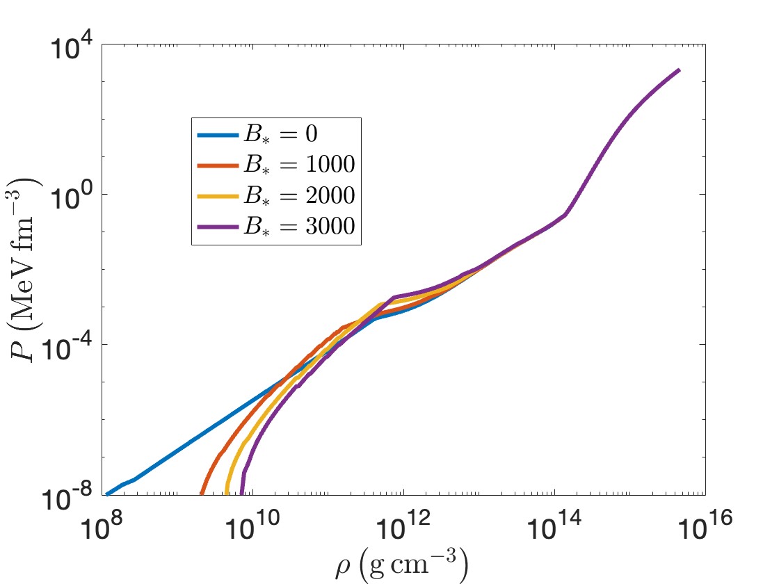
Figure 1: The pressure $P$ is plotted against the energy density $\rho$ for different values of normalized magnetic-field strength $B_{*}\equiv B/B_{\rm rel}$, where $B_{\rm rel}$ is defined in Eq. (17).

III.4 Shear modulus of the crust

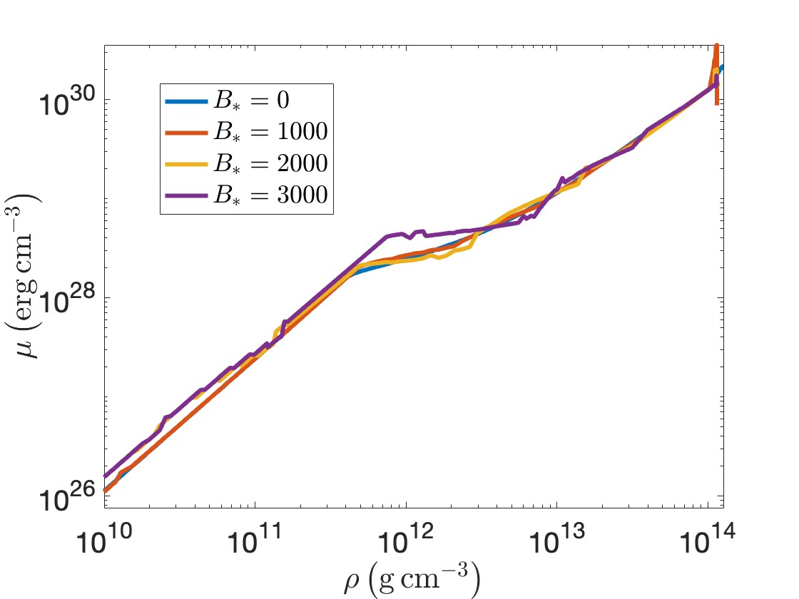
Figure 2: The shear modulus $\mu$ as a function of the energy density $\rho$ for different values of normalized magnetic-field strength $B_{*}\equiv B/B_{\rm rel}$, where $B_{\rm rel}$ is defined in Eq. (17).

The elastic property of the crystallized matter formed by the ions in the neutron star crust treated as an isotropic polycrystal can be characterized by an effective shear modulus $\mu$. Since the shear modulus in the crust is responsible for the restoring force of torsional oscillations, the frequencies of torsional oscillation modes strongly depend on the shear modulus. To compute the torsional modes, an estimation for the shear modulus $\mu$ is required. For practical applications in the neutron star crust, the model of isotropic Coulomb solid [47] is considered and the shear modulus (in CGS system of units) is given by

$$\mu=0.1194\>n_{N}\frac{Z^{2}e^{2}}{a_{i}}.$$ (38)

In Fig. 2, we plot $\mu$ against $\rho$ for our EOS with different values of $B_{*}$.

IV SELF-CONSISTENT STELLAR MODELS

In standard calculations of the torsional modes of magnetized neutron stars (e.g., [14]), one needs to first obtain the spherically symmetric background star by solving the TOV equation. A magnetic field configuration is then imposed and solved for the equilibrium stellar model as discussed in Sec. II.2. However, when the EOS of the crust depends on the magnetic field, so will the structure of the crust. The standard approach is thus not applicable here.

In order to construct a self-consistent equilibrium stellar model that includes the effects of magnetic field on the EOS, we first construct a stellar model without magnetic field and then impose a magnetic field configuration on it just like the standard approach outlined above. Next, with this magnetic field configuration, a new stellar background model is calculated by solving the TOV equation with a magnetic-field-dependent EOS. After that, a new magnetic field configuration is constructed using the new stellar background. This process is repeated until the properties of the star (e.g., the radius $R$ and the crust thickness $\delta r$) converge to some values. When this is achieved, we declare that a self-consistent stellar model is obtained. Our method is summarized by an iteration loop presented in Fig. 3.

As an illustration, Table 1 presents the convergence of $R$ and $\delta r$ after each iteration for a 1.4 $M_{\odot}$ magnetized neutron star with a normal fluid core and a dipole magnetic field having the magnetic field strength of $4\times 10^{16}$ G at the pole of the surface. The convergence will be achieved when the new $\delta r$ only differ from the previous $\delta r$ by less than 0.1%. It is seen that the values of $R$ and $\delta r$ converge rapidly with a few number of iteration cycles only. However, the number of iterations will be greater for stronger magnetic field strengths and more complex magnetic field configurations.

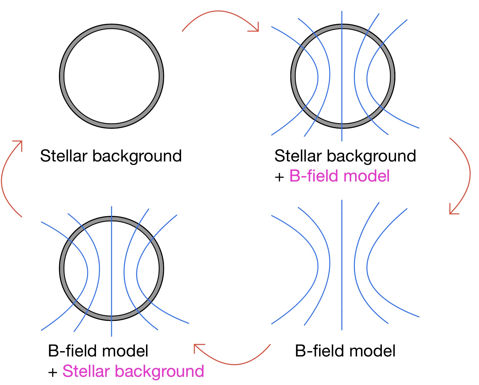
Figure 3: Graphical illustration of the iterative method for the construction of a self-consistent stellar model starting from the upper-left picture. The words in black indicate the information obtained from the previous iteration while those in pink indicate the information to be determined in the current iteration (see text for more details).

Table 1: The values of $M$, $R$ and $\delta r$ for a $1.4M_{\odot}$ neutron star model with a normal fluid core during the iterative calculation of a self-consistent model. The magnetic-field configuration is purely dipole and the field strength at the pole of the surface is $4\times 10^{16}$ G.

No. of cycle	$M/M_{\odot}$	$R$ (km)	$\delta r$ (km)
0	1.40	12.4360	0.8722
1	1.40	12.5426	0.9765
2	1.40	12.5448	0.9786
3	1.40	12.5449	0.9787

In our study, two approximations are made to simplify the problem. Firstly, we assume that the magnetic field has negligible effect on the structure of the fluid core, and hence the fluid core of the star is fixed during the iteration. This should be a good approximation as the EOS at the high-density range relevant to the core is insensitive to the magnetic field for the field strength being considered in this work [23]. It has also been pointed out [33] that the EOS in the core may be affected by the magnetic field only for field strength of the order of $10^{18}$ G, which is beyond our range of consideration.

Secondly, when we solve for the spherically symmetric model using the TOV equation with a magnetic-field-dependent EOS, we make use of the root mean square (r.m.s.) values of the magnetic field $B(r,\theta)$ on any shell of radius $r$. For a given magnetic field configuration, the magnitude of magnetic field in general depends on both the radial and angular positions. In principle, the stellar structure will no longer be spherically symmetric, though the deviation is expected to be very small for the field strength being considered in this work. By using the r.m.s. values of $B\left(r,\theta\right)$, the background stellar model is kept spherically symmetric, but its radius and crust thickness would in general be different from its counterpart without considering the effects of magnetic field on the EOS.

According to our simplified magnetic field models, $B_{\phi}$ is discontinuous at the stellar surface when $\xi>0$, which is unphysical as already noted in Sec. II.2. It is worth to point out that the strength of magnetic field just outside the star is required in the iterative procedure shown in Fig. 3 as the stellar material will extend outward after the effects of magnetic field on the EOS are taken into account. To achieve a more realistic magnetized neutron star model, we extrapolate $B_{\phi}$ outward from the stellar surface so that $B_{\phi}$ will not be discontinuous inside the stellar material within the iterative procedure. The method of extrapolating $B_{\phi}$ outside the star is to keep the corresponding value of $\xi$ (without setting it to be zero as it should be) when the magnitude of $B_{\phi}$ is being calculated using the expression shown in Eq. (10). The r.m.s. values of $B\left(r,\theta\right)$ determined in this way will be more physical near the surface.

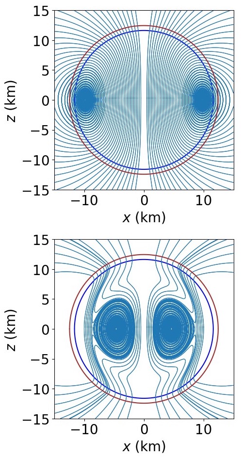
Figure 4: Magnetic field lines on the meridional plane for 1.4 $M_{\odot}$ magnetized neutron stars with a normal fluid core. The upper (lower) panel shows the case for $\xi=0$ (0.45). In each panel, the red and blue circles indicate the stellar surface and the crust-core interface, respectively.

As an illustration, Fig. 4 shows different magnetic field configurations on the meridional plane for 1.4 $M_{\odot}$ neutron stars with a normal fluid core. The upper (lower) panel shows the case for $\xi=0$ (0.45). In each panel, the red and blue circles indicate the stellar surface and the crust-core interface, respectively. One can see that the complexity of the magnetic field configuration increases with $\xi$.

In the following, the variable $B$ will be used to represent the strength of magnetic field at the pole of the stellar surface.

V TORSIONAL OSCILLATIONS

V.1 General-relativistic pulsation equations

For the torsional oscillation modes, the only perturbed fluid variable is the azimuthal component of the perturbed 4-velocity [48]

$$\delta u^{\phi}=\frac{e^{-\nu}}{\sin\,\theta}\frac{\partial Y(r,t)}{\partial t}\frac{dP_{\ell}(\cos\,\theta)}{d\theta},$$ (39)

where $P_{\ell}(\cos\,\theta)$ is the Legendre polynomial of order $\ell$. A harmonic time-dependence is assumed such that the perturbation function $Y(r,t)=Y(r)e^{i\sigma t}$, where $\sigma$ is the angular mode frequency.

In the relativistic Cowling approximation where the metric perturbations are neglected, the equations for determining the torsional oscillation modes can be obtained (see [49, 14] for details) by linearizing the fluid equation and the magnetic induction equation, which is derived from the homogeneous Maxwell’s equations with the ideal Magnetohydrodynamical approximations such that the electric field 4-vector vanishes.

In the following, we briefly summarize the main perturbation equations studied in [14] relevant to our discussion. The perturbed magnetic induction equation is given by

$$\delta\left\{\left(u^{\alpha}H^{\beta}-H^{\alpha}u^{\beta}\right)_{;\>\beta}\right\}=0,$$ (40)

and the perturbed fluid equation is

$$\delta\left(\left[\delta^{j}_{\alpha}+u^{j}u_{\alpha}\right]T^{\alpha\beta}_{\ \ \ \ \ ;\ \beta}\right)=0,$$ (41)

where the spatial index $j=(r,\theta,\phi)$; $T^{\alpha\beta}$ is the stress-energy tensor for the background magnetized neutron star

$$T^{\alpha\beta}=\left(P+\rho+H^{2}\right)u^{\alpha}u^{\beta}+\left(P+\frac{H^{2}}{2}\right)g^{\alpha\beta}-H^{\alpha}H^{\beta},$$ (42)

where $g^{\alpha\beta}$ is the spacetime metric. We assume the background equilibrium star is described by perfect fluid under zero strain, and thus the stress is given by the isotropic pressure. The shear stress due to elasticity only contributes at the perturbative level in Eqs. (40) and (41) after perturbing $T^{\alpha\beta}$ (see [14] for details). To simplify the problem, the $\ell\pm 2$ couplings which appear when Eq. (39) is used to attempt a separation of variables is ignored. The required final pulsation equation obtained from combining Eqs. (40) and (41) is given by [14]

$$\frac{d^{2}Y}{dr^{2}}+\left[\left(1+2\lambda_{1}\right)\frac{a_{1}^{2}}{\mu\pi r^{4}}\right]\frac{d^{2}Y}{dr^{2}}+\left\{\left(\frac{4}{r}+\frac{d\nu}{dr}-\frac{d\lambda}{dr}+\frac{1}{\mu}\frac{d\mu}{dr}\right)+\left(1+2\lambda_{1}\right)\frac{a_{1}}{\mu\pi r^{4}}\left[\left(\frac{d\nu}{dr}-\frac{d\lambda}{dr}\right)a_{1}+2\frac{da_{1}}{dr}\right]\right\}\frac{dY}{dr}$$ (43)

(44)

$$+\left.\right.e^{2\lambda-2\nu}\left[\left(\rho+P\right)\frac{\sigma^{2}}{\mu}-e^{2\nu}\frac{(\ell-1)(\ell+2)}{r^{2}}\right]Y+\left\{\left(1+2\lambda_{1}\right)\frac{a_{1}^{2}}{\mu\pi r^{4}}e^{2\lambda-2\nu}\sigma^{2}-\frac{\lambda_{1}}{2\mu\pi r^{2}}\left(\frac{da_{1}}{dr}\right)^{2}\sigma^{2}e^{-2\nu}\right.$$ (45)

(46)

$$+\left.(\ell-1)(\ell+2)\frac{\lambda_{1}}{2\mu\pi r^{4}}\left(\frac{da_{1}}{dr}\right)^{2}+\left(2+5\lambda_{1}\right)\frac{a_{1}}{2\mu\pi r^{4}}\left[\left(\frac{d\nu}{dr}-\frac{d\lambda}{dr}\right)\frac{da_{1}}{dr}+\frac{d^{2}a_{1}}{dr^{2}}\right]\right\}Y=0,$$ (47)

where $\lambda_{1}=-\frac{\ell(\ell+1)}{(2\ell-1)(2\ell+3)}\>$. Using the variables

$$\begin{split}Y_{1}\equiv Yr^{1-\ell},\;\;\;\;\;\;\;\;\;\;\;\;\;\;\;\;\;\;\;\;\;\;Y_{2}\equiv\left[\mu+\left(1+2\lambda_{1}\right)\frac{a_{1}^{2}}{\pi r^{4}}\right]e^{\nu-\lambda}r^{2-\ell}\frac{dY}{dr},\end{split}$$ (48)

Eq. (43) then becomes two equations in terms of $Y_{1}$ and $Y_{2}$:

$$\frac{dY_{1}}{dr} = -\frac{\ell-1}{r}\>Y_{1}+\frac{\pi r^{3}}{\pi r^{4}\mu+(1+2\lambda_{1})a_{1}^{2}}\>e^{-\nu+\lambda}\>Y_{2},$$ (49)

$$\frac{dY_{2}}{dr} = -\left\{\left[\rho+P+\left(1+2\lambda_{1}\right)\frac{a_{1}^{2}}{\pi r^{4}}-\frac{\lambda_{1}e^{-2\lambda}}{2\pi r^{2}}\left(\frac{da_{1}}{dr}\right)^{2}\right]\sigma^{2}re^{2\left(\lambda-\nu\right)}-(\ell-1)(\ell+2)\left[\frac{\mu e^{2\lambda}}{r}-\frac{\lambda_{1}}{2\pi r^{3}}\left(\frac{da_{1}}{dr}\right)^{2}\right]\right.$$ (53)

$$+\left.(2+5\lambda_{1})\frac{a_{1}e^{2\lambda}}{\pi r^{3}}\left[\frac{a_{1}}{r^{2}}-\frac{\xi^{2}e^{-2\nu}a_{1}}{2}-2\pi f_{0}\left(\rho+P\right)r^{2}\right]\right\}e^{\nu-\lambda}Y_{1}-\frac{\ell+2}{r}Y_{2}.$$

This is the first-order system of equations we solved for the real eigenvalues $\sigma$.

V.2 Boundary conditions

Boundary conditions are needed to be imposed to solve the above system of equations for the mode frequencies. As torsional modes are confined to the crust region, a zero traction condition at the core-crust interface and a zero torque condition at the stellar surface implies that $Y_{2}=0$ at both $r=R-\delta r$ and $r=R$ [14]. However, it should be pointed out that in reality one should also consider the coupling of the crust to the fluid core [16]. In this work, we ignore the coupling with the fluid core to demonstrate the effects of magnetic-field-dependent EOS on the spectrum of torsional modes.

V.3 Code tests

Before studying the effects of Landau-Rabi quantization, we first test the torsional mode frequencies ${}_{\ell}f_{n}$ produced by our code with the results presented in [14, 50, 16], which do not consider the effects of magnetic field on the EOS.

Firstly, the mode frequencies in the non-magnetized limit $\bar{{}_{\ell}f_{n}}$ are tested. Our results were compared with those in [14] for $\bar{{}_{\ell}f_{n}}$ with $n=0,1$ (which is the number of nodes along the coordinate $r$, from the center to stellar surface) and $\ell=2,3,4,...,10$ for their stellar models A+DH_1.4/1.6, WFF3+DH_1.4/1.6, A+NV_1.4/1.6 and WFF3+NV_1.4/1.6. For all the cases, we find that our mode frequencies differ from those reported in [14] by only about 1%, which is much better than similar code tests reported in [15]. The deviations could be due to different numerical treatments of the tabulated EOS data in different codes.

The coefficients ${}_{\ell}\alpha_{n}$ appeared in the following fitting formula proposed in [14]

$$\frac{{}_{\ell}f_{n}}{\bar{{}_{\ell}f_{n}}}=\sqrt{1+{{}_{\ell}\alpha_{n}}\left(\frac{B}{B_{\mu}}\right)^{2}},$$ (54)

for purely dipolar magnetic configurations are also tested with $\ell=2$ and $n=0,1$, where $B_{\mu}=4\times 10^{15}$ G. We again find that the values of ${}_{l}\alpha_{n}$ obtained for the same stellar models tested above differ from the results reported in [14] by only about 1%.

We then tested our mode frequencies ${}_{2}f_{0}$ with mixed poloidal-toroidal magnetic fields. In this part, no numerical data are given in [16]. So we compared our data with the results extracted digitally from the figures presented in [16]. The results are presented in Appendix A.

VI STRUCTURES OF NEUTRON STARS

As mentioned above, having the magnetic-field-dependent EOS, the structure of a neutron star in general varies with the strength and configuration of magnetic field. In this section, we will compare the differences in the stellar structures between models constructed with and without the effects of magnetic field on the EOS. In particular, we focus on the relative differences in $\delta r$ defined by

$$\Delta_{\delta r}=\frac{\delta r^{\prime}-\delta r^{\circ}}{\delta r^{\circ}},$$ (55)

where $\delta r^{\prime}$ is the thickness of the crust after considering the effects of magnetic-field-dependent EOS; $\delta r^{\circ}$ is the original thickness without the effects of magnetic field.

We shall focus on 1.4 $M_{\odot}$ neutron stars as our canonical models in the study. For our chosen BSk24 EOS, a $1.4M_{\odot}$ neutron star has crust thickness $\delta r^{\circ}=0.8722$ km and radius $R^{\circ}=12.4360$ km in the non-magnetized limit. A more massive $2.0M_{\odot}$ model will be considered later in this work.

VI.1 Normal fluid cores

Figure 5: Upper panel: $\Delta_{\delta r}$ as a function of $B$ for $\xi=0$, 0.28 and 0.45. Middle panel: $\xi_{b}$ and $\xi_{c}$ as a function of $B$. Lower panel: $\xi_{a}$ as a function of $B$. Here $B$ is the magnetic-field strength at the pole of a magnetized neutron star, which is assumed to have a normal fluid core.

We first consider the case for normal fluid core and plot $\Delta_{\delta r}$ against the magnetic-field strength $B$ at the pole in the upper panel of Fig. 5. In the figure, three different field configurations $\xi=0$, 0.28, and 0.45 are considered, where $\xi=0$ represents the purely dipole case. It can be seen that $\Delta_{\delta r}$ in general increases with $B$ and $\xi$. Even for a purely dipole field, $\Delta_{\delta r}$ can exceed 10% when the strength of magnetic field is of the order of $10^{16}$ G. For more complex magnetic field configurations with larger values of $\xi$, $\Delta_{\delta r}$ can even exceed 20% when $B$ reaches over $10^{16}$ G. The strength of the magnetic field in the crustal region generally increases with $\xi$ (i.e., a stronger toroidal component) and hence leads to greater effects on the stellar structure via the EOS.

Increasing the crust thickness $\delta r$ also affects the allowed parameter space for physical magnetic-field configurations mentioned in Sec. II.2. In the middle and bottom panels of Fig. 5, we show how the parameters $\xi_{a}$, $\xi_{b}$, and $\xi_{c}$ defined in Eq. (13) change with the field strength $B$. It is seen that $\xi_{b}$ and $\xi_{c}$ remain essentially unchanged. However, $\xi_{a}$ decreases more significantly as $B$ increases. As a result, the gap between the two physical ranges I and II defined in Eq. (13) increases with $B$. It should be noted that as the parameter $\xi$ increases towards the limiting value $\xi_{a}$, the field configuration in general would become more complex. In other words, for physical magnetic-field configurations defined in the physical range I, increasing the field strength $B$ would effectively increase the complexity of the field configuration for a fixed value of $\xi$. Similar effect also exists in the physical range II as it can be seen that its upper limit $\xi_{c}$ also decreases, though not as significant as $\xi_{a}$, when $B$ increases towards $4\times 10^{16}$ G. The consequences of this important effect will be discussed in Sec. VII.

In order to understand why $\Delta_{\delta r}$ is positive and increases with the strength of the magnetic field, we first note that, for the same value of pressure $P$, increasing the field strength will result in a smaller value of energy density $\rho$ near the transition between the inner and outer crustal regions, which happens at the density range between about $5\times 10^{11}\ {\rm g\ cm}^{-3}$ and $10^{12}\ {\rm g\ cm}^{-3}$ for different field strengths shown in Fig. 1. According to Eq. (2), a smaller value of $\rho$ leads to a smaller value of $|dP/dr|$, and hence a flatten density profile which can extend further away until it reaches the surface.

To illustrate this phenomenon, we show the normalized energy-density profiles (blue lines) and pressure profiles (yellow lines) in the crustal region for three different star models in Fig. 6. The solid lines represent the profiles for a unmagnetized neutron star. The dotted lines are the profiles for a magnetized star with a purely dipole field ($\xi=0$) and $B=4\times 10^{16}$ G, which branch off from the solid lines leading to a thicker crust. However, the dotted lines in fact drop more rapidly near the stellar surface comparing to the solid lines. This can be understood from Fig. 1 that increasing the field strength for a fixed pressure leads to a higher density at the low density region, and hence a steeper $|dP/dr|$ near the surface. One can also see from Fig. 6 that, for the same field strength $B$ at the pole, increasing the value of $\xi$ from 0 to 0.28 (dashed lines) can further increase the thickness of the crust.

Figure 6: The profiles of energy density $\rho$ and pressure $P$ normalized by their own values $\rho_{\rm crust}$ and $P_{\rm crust}$, respectively, at the base of the crust. The solid lines represent the profiles for an unmagnetized neutron star. The dotted and dashed lines are the profiles for magnetized stars with the same magnetic field strength $B=4\times 10^{16}$ G, but with different field configurations $\xi=0$ and 0.28.

VI.2 Superconducting cores

Figure 7: Upper panel: $\Delta_{\delta r}$ as a function of $B$ for $\xi=0$, 0.9, 1.1 and 1.2. Lower panel: $\xi_{\gamma}$ as a function of $B$. The neutron star is assumed to have a superconducting core and the magnetic field is confined in the crust.

For neutron stars with a superconducting core, $\Delta_{\delta r}$ also increases with $B$ and $\xi$ as shown in the upper panel of Fig. 7. However, $\Delta_{\delta r}$ now becomes more sensitive to the field strength comparing to the case of normal fluid core. For neutron stars with a normal fluid core, $\Delta_{\delta r}$ increases to about 5% for $\xi=0.45$ and $B=4\times 10^{15}$ G as shown in Fig. 5. For the same value of $B$, superconducting-core models can reach up to 10% when $\xi\approx 1$. The bottom panel of Fig. 7 shows that the parameter $\xi_{\gamma}$, which defines the physical range of parameter in Eq. (15), also decreases with increasing $B$.

VII MODE FREQUENCIES

As mentioned above, the torsional oscillation modes ${}_{\ell}f_{n}$ for neutron stars with mixed poloidal-toroidal magnetic fields, but without considering the effect of Landau-Rabi quantization, have been studied [15]. In this work, we only focus on the $\ell=2$ fundamental torsional oscillation modes and investigate the changes in the mode frequencies when the effect of magnetic field on the EOS is considered. We define the relative differences in mode frequencies by

$$\Delta_{f}=\frac{{f}^{\prime}-f^{\circ}}{f^{\circ}},$$ (56)

where $f^{\prime}$ and $f^{\circ}$ are the frequencies calculated with and without the effect of magnetic field on the EOS, respectively.

VII.1 Normal fluid cores

In the upper panel of Fig. 8, we plot $f^{\prime}$ (dotted lines) and $f^{\circ}$ (solid lines) against $B$ for neutron stars with a normal fluid core and magnetic field configurations defined by $\xi=0$, 0.28 and 0.45. One can observe that $f^{\circ}$ increases rapidly with $B$ and $\xi$ when the field strength is larger than about $10^{15}$ G. This phenomenon has been discussed in [14, 15]. A semi-analytical understanding is provided in Appendix B. Including the effect of magnetic field on the EOS (dotted lines), the mode frequency further increases for fixed values of $B$ and $\xi$. The difference between $f^{\prime}$ and $f^{\circ}$ also increases with the complexity (i.e., the value of $\xi$) of the field configuration. The difference $\Delta_{f}$ is plotted in the lower panel of Fig. 8. For $B=4\times 10^{15}$ G, $\Delta_{f}$ can reach only up to a few percent even for the case $\xi=0.45$, which is already near the upper limit of the physical range II defined in Eq. (13). However, $\Delta_{f}$ can rise up to about 10% when the field strength $B\approx 2\times 10^{16}$ G for $\xi=0.28$ and 0.45. For the case of purely dipole field ($\xi=0$), $\Delta_{f}$ can reach only up to about 5% even when $B=4\times 10^{16}$ G. As discussed in Sec. VI, for a fixed value of $\xi$, including the effect of magnetic field on the EOS would effectively increase the complexity of the field configuration, and hence leading to the increase of $\Delta_{f}$ as $B$ increases.

Figure 8: Upper panel: Mode frequency $f$ as a function of $B$ for $\xi=0$, 0.28 and 0.45. The solid lines correspond to $f^{\circ}$, while the dotted lines correspond to $f^{\prime}$. Lower panel: $\Delta_{f}$ as a function of $B$. The neutron star is assumed to have a normal fluid core and the magnetic field extends throughout the star.

VII.2 Superconducting cores

For neutron stars with a superconducting core, the results differ from the above results qualitatively. Similar to Fig. 8, we plot $f^{\circ}$ and $f^{\prime}$ in the upper panel of Fig. 9 to illustrate how the mode frequencies change with $B$ and $\xi$. In this case, it is seen that $f^{\circ}$ increases with $B$ but decreases with $\xi$. Hence, in contrast to neutron stars with a normal fluid core, increasing the complexity of the field configuration (i.e., the value of $\xi$) would decrease the mode frequency. A semi-analytical understanding is provided in Appendix B.

Again, as discussed in Sec. VI, including the effect of magnetic field on the EOS effectively increases the complexity of the field configuration for a fixed value of $\xi$, since the upper limit $\xi_{\gamma}$ of the physical range defined in Eq. (15) decreases with increasing $B$. This is why the frequency $f^{\prime}$ is smaller than $f^{\circ}$ for given values of $B$ and $\xi$. The difference $\Delta_{f}$ between the two frequencies increases with $B$ and $\xi$ as shown in the lower panel of Fig. 9. In particular, the magnitude of $\Delta_{f}$ can reach up to about 20% when $B=4\times 10^{15}$ G for the case $\xi=1.2$, which is close to the upper limit of $\xi_{\gamma}$ as shown in Fig. 7.

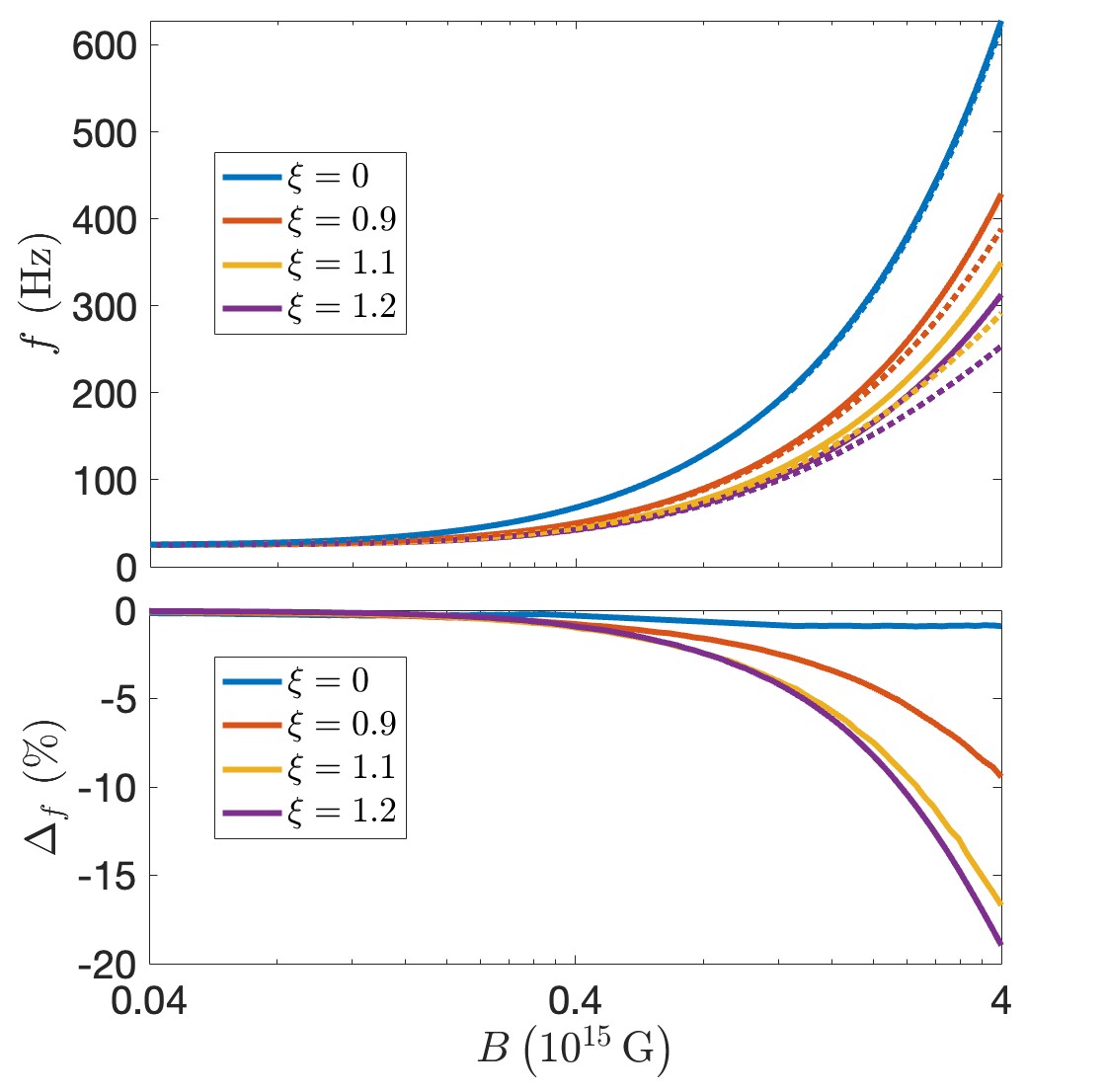
Figure 9: Upper panel: $f$ as a function of $B$ for $\xi=0$, 0.9, 1.1 and 1.2. The solid and dotted lines correspond to $f^{\circ}$ and $f^{\prime}$, respectively. Lower panel: $\Delta_{f}$ as a function of $B$. The neutron star is assumed to have a superconducting core and the magnetic field is confined in the crust.

VIII Effects of stellar mass

So far we have focused on a $1.4M_{\odot}$ neutron star. Let us now present the results for a more massive $2.0M_{\odot}$ model with $\delta r^{\circ}=0.4615$ km and $R^{\circ}=12.2298$ km in the non-magnetized limit. We shall see how $\Delta_{\delta r}$ and $\Delta_{f}$ change for neutron stars with different masses. It is worth noticing that the mode frequency $f^{\circ}$ for a $2.0M_{\odot}$ neutron star model is not the same as that of the $1.4M_{\odot}$ model. For comparison, we also present the corresponding values of $\xi_{a},\xi_{b},\xi_{c}$ and $\xi_{\gamma}$ for $1.4M_{\odot}$ and $2.0M_{\odot}$ neutron star models in the weak field limit ($B\ll 10^{15}$ G) in Table 2.

VIII.1 Normal fluid cores

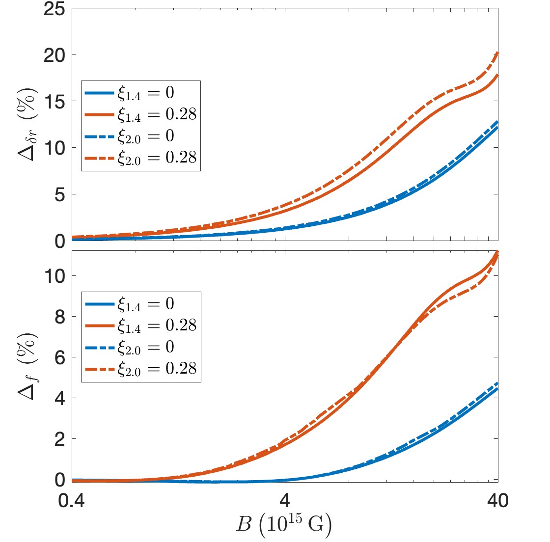
Figure 10: Upper panel: $\Delta_{\delta r}$ as a function of $B$ for $\xi=0$ (blue lines) and 0.28 (red lines). Lower panel: $\Delta_{f}$ as a function of $B$. The solid and dotted-dashed lines correspond to neutron star models with $1.4M_{\odot}$ and $2.0M_{\odot}$, respectively. The neutron stars are assumed to have a normal fluid core, and the magnetic field extends throughout the stars.

Table 2: The values of $\xi_{a},\xi_{b},\xi_{c}$ and $\xi_{\gamma}$ for $1.4M_{\odot}$ and $2.0M_{\odot}$ neutron star models in the weak field limit ($B\ll 10^{15}$ G).

$M/M_{\odot}$	$\xi_{a}$	$\xi_{b}$	$\xi_{c}$	$\xi_{\gamma}$
1.4	0.298	0.354	0.462	1.4
2.0	0.255	0.265	0.365	2.1

We first compare how the differences in the thickness of the crust $\Delta_{\delta r}$ defined in Eq. (55), relative to the nonmagnetic limit, depend on the stellar mass in the upper panel of Fig. 10. In the figure, the blue lines correspond to the purely dipole field configuration ($\xi=0$) for star models with $1.4M_{\odot}$ (solid line) and $2.0M_{\odot}$ (dotted-dashed line). It is seen that the two lines agree quite well with each other even up to $B=4\times 10^{16}$ G, and hence $\Delta_{\delta r}$ is insensitive to the stellar mass for $\xi=0$. For a more complex field configuration defined by $\xi=0.28$ (red lines), the results are slightly more sensitive to the stellar mass. Similarly, we plot the corresponding differences in the mode frequency $\Delta_{f}$ in the lower panel of Fig. 10 and notice that $\Delta_{f}$ is somewhat less sensitive to the stellar mass for $\xi=0.28$ comparing to $\Delta_{\delta r}$.

VIII.2 Superconducting cores

For neutron stars with a superconducting core, the effects of stellar mass are different from those discussed above. Similar to Fig. 10, we consider how $\Delta_{\delta r}$ depends on stellar mass in the upper panel of Fig. 11. The yellow (blue) lines indicate the results for stellar models constructed by the field configuration $\xi=0.9$ ($\xi=1.1$). The $1.4M_{\odot}$ and $2.0M_{\odot}$ models are represented by the solid and dotted-dashed lines, respectively. Unlike the situation for a normal fluid core, it is seen that $\Delta_{\delta r}$ is now more sensitive to the stellar mass as the blue solid and dotted-dashed lines, and similarly for the yellow lines, already deviate from each other significantly when $B=4\times 10^{15}\textrm{G}$. Nevertheless, $\Delta_{\delta r}$ in general increases with the stellar mass for both normal fluid and superconducting cores. In the lower panel of Fig. 11, we plot the corresponding $\Delta_{f}$ for neutron stars with a superconducting core. In contrast to the case for a normal fluid core, where $\Delta_{f}$ is weakly dependent on the stellar mass, it is seen that $\Delta_{f}$ now depends more sensitively on the stellar mass. In particular, the magnitude of $\Delta_{f}$ increases with decreasing stellar mass for a given magnetic field strength.

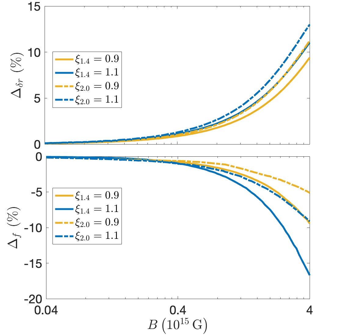
Figure 11: Upper panel: $\Delta_{\delta r}$ as a function of $B$ for $\xi=0.9$ (yellow lines) and 1.1 (blue lines). Lower panel: $\Delta_{f}$ as a function of $B$. The solid and dotted-dashed lines correspond to neutron star models with $1.4M_{\odot}$ and $2.0M_{\odot}$, respectively. The neutron stars are assumed to have a superconducting core, and the magnetic field is confined in the crust.

IX Discussion

The intense magnetic field of a magnetar can affect the structure and EOS of the crust of the star. In this paper, we have studied the effects of Landau-Rabi quantization of electron motion on the crustal torsional oscillations of magnetars under the Cowling approximation. For the EOS model, we employ the study of [23] which incorporates the effects of Landau-Rabi quantization by treating the inner and outer crusts consistently based on the nuclear-energy density functional theory. We also consider mixed poloidal-torodial magnetic field configurations for our stellar models. In our study, the magnetic field configuration first contributes to the calculation of the torsional oscillation modes through its effect on the magnetic-field-dependent EOS due to the Landau-Rabi quantization, and hence the resulting self-consistent stellar model as discussed in Sec. IV. The magnetic field then contributes at the level of the perturbation equations that determine the oscillation modes. We assume spherically symmetric stellar models and ignore the crust deformation [51] and the modification of the energy-momentum tensor due to the strong magnetic field [33]. These effects are expected to be non-negligible only when the strength of magnetic field is of the order of $10^{18}$ G, which is far beyond our range of study here and the typical strength of magnetic field of magnetars.

The magnetic field configurations are characterized by the strength of the magnetic field $B$ at the pole of the stellar surface and the parameter $\xi$, which represents the ratio between the toroidal and poloidal components of the magnetic field. Our numerical results show that the crust thickness $\delta r$ increases with both $B$ and $\xi$ when the effect of magnetic field is considered in the EOS. For a more complex magnetic field configuration with a nonzero $\xi$, $\delta r$ can increase by more than 20% when $B\sim 10^{16}$ G for neutron stars with a normal fluid core. On the other hand, for neutron stars with a superconducting core, $\delta r$ can already increase by 10% when $B\sim 10^{15}$ G.

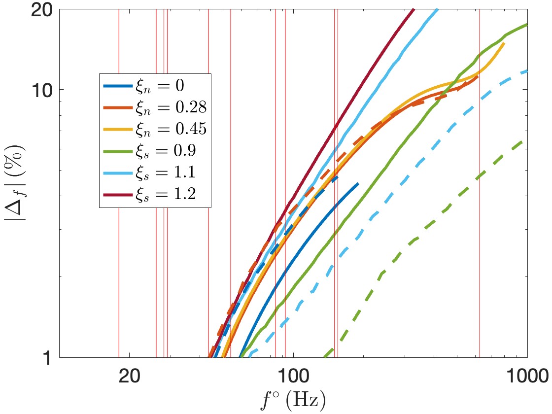
Figure 12: $\left|\Delta_{f}\right|$ as a function of $f^{\circ}$ for different models. The subscripts $n$ and $s$ in the parameter $\xi$ indicate that the neutron star models consists of a normal fluid and superconducting core, respectively. The solid lines and dashed lines represent the results for 1.4 $M_{\odot}$ and 2.0 $M_{\odot}$ neutron star models, respectively. The vertical lines denote some of the observed QPO frequencies in magnetar giant flares.

We focus on the fundamental $\ell=2$ torsional oscillation modes and study the changes in the mode frequencies when the effect of the magnetic field on the EOS is incorporated. It is found that the magnitude of the fractional change in mode frequency $\left|\Delta_{f}\right|$ increases with $B$ and $\xi$. For the models that we have considered, $|\Delta_{f}|$ can exceed 10% when $B\sim 10^{16}$ G for neutron stars with a normal fluid core. For neutron stars with a superconducting core, however, $|\Delta_{f}|$ can even approach 20% at a smaller field strength $B\sim 10^{15}$ G, which lies at the top end of the observed range of magnetic field for magnetars. It is also worth to note that $\Delta_{f}$ is positive (negative) for neutron stars with a normal fluid (superconducting) core, and hence the effect of Landau-Rabi quantization would increase (decrease) the mode frequency correspondingly. We have also studied the effect of stellar mass and found that $\Delta_{f}$ is not sensitive to the stellar mass for models with a normal fluid core. However, for a superconducting core, $\Delta_{f}$ depends more sensitively on the stellar mass and increases with decreasing mass, especially for field strength larger than $B\sim 10^{15}$ G.

Let us now put together the results of all the stellar models studied in this work and discuss the implication from an observational perspective. While the mechanism for the magnetar giant flares and the identities of the observed QPOs in the late-time tail phase are still not well understood, it is believed that the magneto-elastic oscillations of the star must play a role. Although whether the torsional oscillation modes of magnetars could explain (at least) some of the observed QPOs is far from clear, let us use this simplest scenario as an example to illustrate the implication of our numerical results. In particular, we want to address under what situation we need to worry about the effect of Landau-Rabi quantization and the level of deviations one could have if the effect is not considered in the theoretical calculation of the oscillation modes, when comparing to the observed data.

In Fig. 12, we plot $\left|\Delta_{f}\right|$ as a function of the mode frequencies $f^{\circ}$ without considering the effect of magnetic field on the EOS for different models studied in this work, where the subscripts $n$ and $s$ in the parameter $\xi$ indicate that the neutron star models consist of a normal fluid and superconducting core, respectively. The solid and dashed lines with the same color represent $1.4M_{\odot}$ and $2.0M_{\odot}$ models for the same value of $\xi$, respectively. In addition, the vertical lines denote the frequencies of some of the observed QPO as mentioned in Sec. I. Figure 12 shows that the effect of Landau-Rabi quantization is not important when one considers the observed QPOs with smaller frequencies ($\lesssim 80$ Hz), but becomes relevant for higher frequencies modes. It can be seen that $\left|\Delta_{f}\right|$ is always less than 1% for $f^{\circ}$ being around 40 Hz. However, $\left|\Delta_{f}\right|$ exceeds 3% for $f$ being around 90 Hz and approaching 10% for $f$ being around 150 Hz.

In addition, one can see that different models show similar trends in Fig. 12, which can be fitted approximately by

$$\left|\Delta_{f}\right|=K\left(f^{\circ}\right)^{1.12\pm 0.12},$$ (57)

where $K$ is a constant depending on the background star model. This fit applies to the range for $\left|\Delta_{f}\right|$ being between 1% and 10%. On the other hand, we plot $\left|\Delta_{f}\right|$ against $\Delta_{\delta_{r}}$ in Fig. 13. As one may expected, there should be some correlation between the two quantities. Different models also show similar trends in Fig. 13, which can be fitted for $\Delta_{\delta r}$ in the range between 2% and 10% approximately by

$$\left|\Delta_{f}\right|=K^{\prime}\left(\Delta_{\delta r}\right)^{1.11\pm 0.04},$$ (58)

where $K^{\prime}$ is a constant depending on the background star model.

Figure 13: $\left|\Delta_{f}\right|$ as a function of $\Delta_{\delta r}$ for different models, similar to Fig. 12.

In conclusion, depending on the star models and magnetic field configurations, we have shown that the effect of Landau-Rabi quantization of electron motion in the crust can change the frequencies of the fundamental torsional oscillation modes by up to 10% to 20% for magnetic field strength $B\sim 10^{15}-10^{16}$ G, which is within the measured surface field strength of magnetars. Our work provides a benchmark on the parameter space of stellar models and observation precision within which one needs to consider the Landau-Rabi quantization. In the future, we plan to extend our study to other oscillation modes such as the interfacial and shear modes, which also depend sensitively on the properties of the solid crust and may also be excited in magnetar starquakes.

Appendix A CODE TESTS WITH MIXED POLOIDAL-TOROIDAL MAGNETIC FIELDS

In this appendix, we verify our code by comparing our numerical results for torsional oscillation modes with mixed poloidal-toroidal magnetic field configurations with the data published in [16]. We consider their 1.4 $M_{\odot}$ stellar model described by the following EOS:

$$P=0.00936n_{0}m_{b}\left(\frac{\bar{n}}{n_{0}}\right)^{2.46},$$ (59)

$$\rho=\bar{n}m_{b}+\frac{P}{1.46},$$ (60)

$$\mu=\rho v_{s}^{2},$$ (61)

where $n_{0}=0.1\,\textrm{fm}^{-3}$, $m_{b}=1.66\times 10^{-24}\textrm{g}$ and $v_{s}=\sqrt{\mu/\left(\rho+P\right)}$ is the velocity of the shear wave as measured by a local observer which is assumed here to be fixed at its typical value of $10^{8}\,\textrm{cm\,s}^{-1}$ [48]. In the upper panel of Fig. 14, we plot the fundamental torsional oscillation mode frequencies $f$ against the normalized magnetic field strength $B/B_{\mu}(B_{\mu}=4\times 10^{15}{\ \rm G})$ for this background star with a normal fluid core and magnetic field configurations defined by $\xi=0.1$ and 0.31. The solid lines are the results extracted from the figures in [16] and the dots are our numerical results. Similarly, the lower panel of Fig. 14 shows the comparison for neutron stars with a superconducting core and magnetic field configurations defined by $\xi=0.8$ and 1.9. We see that our results match those presented in [16] very well.

Figure 14: Comparison between our numerical results (data points) and the results (solid lines) presented in [16] for a $1.4M_{\odot}$ neutron star model with different magnetic field configurations (see text for more details). The upper (lower) panel plots the fundamental torsional oscillation mode frequency $f$ against the normalized field strength $B/B_{\mu}$ for the case of a normal fluid (superconducting) core.

Appendix B SEMI ANALYTICAL UNDERSTANDING OF TORSIONAL OSCILLATION MODES WITH MIXED POLOIDAL-TOROIDAL MAGNETIC FIELDS

To understand the behaviours of the torsional oscillation mode frequency $f$ with mixed poloidal-toroidal magnetic fields, we can apply approximations on Eq. (43). In this appendix, we do not consider the effects of magnetic field on the EOS.

B.1 Normal fluid core

Let us first consider neutron stars with a normal fluid core. To simplify the problem, we only focus on the Newtonian limit. As the torsional oscillations are confined in the solid crust, we only need to analyze the crustal region. In addition, we assume a thin crust and a constant shear speed throughout the region. For a thin crust, we have $d^{2}Y/dr^{2}\approx dY/dr\approx 0$ in our analysis due to the boundary conditions at the base of the crust and the stellar surface, which require $Y_{2}=dY/dr=0$.

As we are only interested in how the mode angular frequency $\sigma$ scales with the magnetic field strength $B$ and the parameter $\xi$ qualitatively, we can perform an order-of-magnitude approximation for Eq. (43) and obtain, after using Eq. (9), the following result:

$$\begin{split}\sigma^{2}\approx&\frac{(\ell-1)(\ell+2)}{R^{2}}v_{s}^{2}\\ &+\frac{2+5\lambda_{1}}{2\pi\left\langle\rho\right\rangle R^{4}}\left[\left\langle 2\left(2\pi f_{0}\rho R^{2}a_{1}-\frac{a_{1}^{2}}{R^{2}}\right)\right\rangle+\xi^{2}\left\langle a_{1}^{2}\right\rangle\right],\end{split}$$ (62)

where $\left\langle x\right\rangle$ is the average value of $x$ throughout the crust. In the absence of magnetic field (i.e., $a_{1}=0$), we obtain the non-magnetic eigenvalue $\sigma^{2}\approx{\bar{\sigma}}^{2}\equiv(\ell-1)(\ell+2)v_{s}^{2}/R^{2}$, which agrees with the result obtained in [52] except that a metric function of order unity is ignored in our analysis. We thus have

$$\begin{split}\frac{\sigma^{2}}{\bar{\sigma}^{2}}\approx 1+\frac{2+5\lambda_{1}}{2\pi\bar{\sigma}^{2}\left\langle\rho\right\rangle R^{4}}\left[\left\langle 2\left(2\pi f_{0}\rho R^{2}a_{1}-\frac{a_{1}^{2}}{R^{2}}\right)\right\rangle+\xi^{2}\left\langle a_{1}^{2}\right\rangle\right].\end{split}$$ (63)

From Eq. (9), one sees that $\left|2\pi f_{0}\rho R^{2}\right|>\left|a_{1}/R^{2}\right|$ throughout the crust (as $d^{2}a_{1}/dr^{2}\approx 0$ and $da_{1}/dr<0$ from Eq. (11)). On the other hand, the source term $f_{0}\left(\rho+P\right)R^{2}$ in Eq. (9) scales like $B$, as that is the current distribution producing the magnetic field. As $a_{1}\propto B$ at the surface, we can approximate $\left\langle a_{1}^{2}\right\rangle\propto B^{2}$ and obtain the final relation

$$\begin{split}\frac{\sigma^{2}}{\bar{\sigma}^{2}}=1+C_{\ell}B^{2}+D_{\ell}B^{2}\xi^{2},\end{split}$$ (64)

where $C_{l}$ and $D_{l}$ are some positive constants depending on $\ell$ and the stellar models. Rewriting the terms give

$$\begin{split}\frac{\sigma}{\bar{\sigma}}=\left[1+C_{\ell}(1+E_{\ell}\xi^{2})B^{2}\right]^{1/2},\end{split}$$ (65)

where $E_{\ell}=D_{\ell}/C_{\ell}$. This is exactly the results provided numerically in [15]. For purely dipole field ($\xi=0$), it reduces to the fitting formula proposed in [14] (i.e., Eq. (54)).

B.2 Superconducting core

As stated in [16], the $\theta$-component of magnetic field will be much stronger than the other components when the magnetic field is confined only in the crustal region. So, here we repeat the same analysis above but keep the terms with $da_{1}/dr$ instead of $a_{1}$ (see Eq. (10)). The final result can be written as

$$\begin{split}\frac{\sigma^{2}}{\bar{\sigma}^{2}}\approx 1+C_{\ell}B^{2}+F_{\ell}\left\langle\left(\frac{da_{1}}{dr}\right)^{2}\right\rangle,\end{split}$$ (66)

where $F_{\ell}=\left(\ell-1\right)\left(\ell+2\right)\left(\frac{\left|\lambda_{1}\right|}{2\pi\bar{\sigma}^{2}\left\langle\rho\right\rangle R^{4}}\right)$. Applying similar approximations as above and only considering the cases with $\xi\sim 1$ for our numerical results, Eq. (9) can be approximated by

$$\begin{split}\frac{d^{2}a_{1}}{dr^{2}}+\frac{2M}{R^{2}}\frac{da_{1}}{dr}+\xi^{2}a_{1}\approx\Gamma B,\end{split}$$ (67)

where $\Gamma$ is some constant depending on the stellar model. We have also neglected the term $2a_{1}/r^{2}$ in Eq. (9) in the analysis as it is much smaller than the other terms near the surface. In the following, $M/R^{2}$ will be taken as $0.01$ in our order-of-magnitude analysis. Solving this second-order ordinary differential equation, we obtain approximately

$$\begin{split}a_{1}\left(r\right)\approx\chi_{1}e^{-0.01r}\sin\left(\xi r\right)+\chi_{2}e^{-0.01r}\cos\left(\xi r\right)+\frac{\Gamma B}{\xi^{2}},\end{split}$$ (68)

where $\chi_{1}$ and $\chi_{2}$ are some constants. By requiring $a_{1}\left(R-\delta r\right)=\frac{d^{2}a_{1}}{dr^{2}}\left(R-\delta r\right)=0$ (see Sec. II.2 for the boundary conditions), both $\chi_{1}$ and $\chi_{2}$ scale like $B/\xi^{2}$. As a result,

$$\begin{split}\left\langle\frac{da_{1}}{dr}\right\rangle\propto\frac{B}{\xi}.\end{split}$$ (69)

Eq. (66) can then be expressed as

$$\begin{split}\frac{\sigma^{2}}{\bar{\sigma}^{2}}=1+C_{\ell}B^{2}+G_{\ell}\frac{B^{2}}{\xi^{2}},\end{split}$$ (70)

where $G_{\ell}$ is some constant depending on $\ell$ and the stellar model. We have tested this relation with our numerical results to verify that the $\xi$-dependence obtained is valid and the error is less than 10% for the range of magnetic field strength considered. Therefore, given a fixed value of $B$, increasing the value of $\xi$ will decrease $\sigma$.

For the cases with $\xi=0$, the solution of Eq. (67) is given approximately by

$$\begin{split}a_{1}\left(r\right)\approx\chi_{1}e^{-0.01r}+\chi_{2}+100\Gamma Br.\end{split}$$ (71)

Again, having $a_{1}\left(R-\delta r\right)=\frac{d^{2}a_{1}}{dr^{2}}\left(R-\delta r\right)=0$, we determine that $\chi_{1}=0$ and $\chi_{2}$ is just some constant. Therefore, we have $\left\langle\frac{da_{1}}{dr}\right\rangle\propto B$ and

$$\begin{split}\frac{\sigma^{2}}{\bar{\sigma}^{2}}=1+J_{\ell}B^{2},\end{split}$$ (72)

where $J_{\ell}$ is some constant depending on $l$ and the stellar model. This relation has been tested with our numerical results and the error is around 1% only.

References

- Shapiro and Teukolsky [1983] S. Shapiro and S. Teukolsky, Black holes, white dwarfs, and neutron stars: The physics of compact objects. (Wiley Interscience, New York, 1983).
- Turolla et al. [2015] R. Turolla, S. Zane, and A. L. Watts, Magnetars: the physics behind observations. a review, Rep. Prog. Phys. 78, 116901 (2015).
- Kaspi and Beloborodov [2017] V. M. Kaspi and A. M. Beloborodov, Magnetars, Annual Review of Astronomy and Astrophysics 55, 261 (2017), arXiv:1703.00068 [astro-ph.HE] .
- Rea and Esposito [2011] N. Rea and P. Esposito, Magnetar outbursts: an observational review, in High-Energy Emission from Pulsars and their Systems, Astrophysics and Space Science Proceedings, Vol. 21 (2011) p. 247, arXiv:1101.4472 [astro-ph.GA] .
- Hurley et al. [1999] K. Hurley, T. Cline, E. Mazets, S. Barthelmy, P. Butterworth, F. Marshall, D. Palmer, R. Aptekar, S. Golenetskii, V. Il’Inskii, D. Frederiks, J. McTiernan, R. Gold, and J. Trombka, A giant periodic flare from the soft -ray repeater SGR1900+14, Nature (London) 397, 41 (1999), arXiv:astro-ph/9811443 [astro-ph] .
- Hurley et al. [2005] K. Hurley, S. E. Boggs, D. M. Smith, R. C. Duncan, R. Lin, A. Zoglauer, S. Krucker, G. Hurford, H. Hudson, C. Wigger, W. Hajdas, C. Thompson, I. Mitrofanov, A. Sanin, W. Boynton, C. Fellows, A. von Kienlin, G. Lichti, A. Rau, and T. Cline, An exceptionally bright flare from SGR 1806-20 and the origins of short-duration -ray bursts, Nature (London) 434, 1098 (2005), arXiv:astro-ph/0502329 [astro-ph] .
- Mereghetti et al. [2005] S. Mereghetti, D. Götz, A. von Kienlin, A. Rau, G. Lichti, G. Weidenspointner, and P. Jean, The First Giant Flare from SGR 1806-20: Observations Using the Anticoincidence Shield of the Spectrometer on INTEGRAL, Astrophys. J. Lett. 624, L105 (2005), arXiv:astro-ph/0502577 [astro-ph] .
- Israel et al. [2005] G. L. Israel, T. Belloni, L. Stella, Y. Rephaeli, D. E. Gruber, P. Casella, S. Dall’Osso, N. Rea, M. Persic, and R. E. Rothschild, The Discovery of Rapid X-Ray Oscillations in the Tail of the SGR 1806-20 Hyperflare, Astrophys. J. Lett. 628, L53 (2005), arXiv:astro-ph/0505255 [astro-ph] .
- Watts and Strohmayer [2006] A. L. Watts and T. E. Strohmayer, Detection with RHESSI of High-Frequency X-Ray Oscillations in the Tailof the 2004 Hyperflare from SGR 1806-20, Astrophys. J. Lett. 637, L117 (2006), arXiv:astro-ph/0512630 [astro-ph] .
- Strohmayer and Watts [2006] T. E. Strohmayer and A. L. Watts, The 2004 Hyperflare from SGR 1806-20: Further Evidence for Global Torsional Vibrations, Astrophys. J. 653, 593 (2006), arXiv:astro-ph/0608463 [astro-ph] .
- Strohmayer and Watts [2005] T. E. Strohmayer and A. L. Watts, Discovery of Fast X-Ray Oscillations during the 1998 Giant Flare from SGR 1900+14, Astrophys. J. Lett. 632, L111 (2005), arXiv:astro-ph/0508206 [astro-ph] .
- Barat et al. [1983] C. Barat, R. I. Hayles, K. Hurley, M. Niel, G. Vedrenne, U. Desai, V. G. Kurt, V. M. Zenchenko, and I. V. Estulin, Fine time structure in the 1979 March 5 gamma ray burst, Astron. Astrophys. 126, 400 (1983).
- Castro-Tirado et al. [2021] A. J. Castro-Tirado, N. Østgaard, E. Göǧüş, C. Sánchez-Gil, J. Pascual-Granado, V. Reglero, A. Mezentsev, M. Gabler, M. Marisaldi, T. Neubert, C. Budtz-Jørgensen, A. Lindanger, D. Sarria, I. Kuvvetli, P. Cerdá-Durán, J. Navarro-González, J. A. Font, B. B. Zhang, N. Lund, C. A. Oxborrow, S. Brandt, M. D. Caballero-García, I. M. Carrasco-García, A. Castellón, M. A. Castro Tirado, F. Christiansen, C. J. Eyles, E. Fernández-García, G. Genov, S. Guziy, Y. D. Hu, A. Nicuesa Guelbenzu, S. B. Pandey, Z. K. Peng, C. Pérez del Pulgar, A. J. Reina Terol, E. Rodríguez, R. Sánchez-Ramírez, T. Sun, K. Ullaland, and S. Yang, Very-high-frequency oscillations in the main peak of a magnetar giant flare, Nature (London) 600, 621 (2021).
- Sotani et al. [2007] H. Sotani, K. D. Kokkotas, and N. Stergioulas, Torsional oscillations of relativistic stars with dipole magnetic fields, Mon. Not. R. Astron. Soc. 375, 261 (2007), arXiv:astro-ph/0608626 [astro-ph] .
- de Souza and Chirenti [2019] G. H. de Souza and C. Chirenti, Torsional oscillations of magnetized neutron stars with mixed poloidal-toroidal fields, Phys. Rev. D 100, 043017 (2019), arXiv:1810.06628 [astro-ph.HE] .
- Sotani et al. [2008] H. Sotani, A. Colaiuda, and K. D. Kokkotas, Constraints on the magnetic field geometry of magnetars, Mon. Not. R. Astron. Soc. 385, 2161 (2008).
- Levin [2006] Y. Levin, QPOs during magnetar flares are not driven by mechanical normal modes of the crust, Mon. Not. R. Astron. Soc. 368, L35 (2006), arXiv:astro-ph/0601020 [astro-ph] .
- Gabler et al. [2011] M. Gabler, P. Cerdá Durán, J. A. Font, E. Müller, and N. Stergioulas, Magneto-elastic oscillations and the damping of crustal shear modes in magnetars, Mon. Not. R. Astron. Soc. 410, L37 (2011), arXiv:1007.0856 [astro-ph.HE] .
- Rabi [1928] I. v. Rabi, Das freie elektron im homogenen magnetfeld nach der diracschen theorie, Zeitschrift für Physik 49, 507 (1928).
- Landau [1930] L. Landau, Diamagnetismus der metalle, Zeitschrift für Physik 64, 629 (1930).
- Chamel et al. [2012] N. Chamel, R. L. Pavlov, L. M. Mihailov, C. J. Velchev, Z. K. Stoyanov, Y. D. Mutafchieva, M. D. Ivanovich, J. M. Pearson, and S. Goriely, Properties of the outer crust of strongly magnetized neutron stars from hartree-fock-bogoliubov atomic mass models, Phys. Rev. C 86, 055804 (2012).
- Chamel et al. [2015a] N. Chamel, Z. K. Stoyanov, L. M. Mihailov, Y. D. Mutafchieva, R. L. Pavlov, and C. J. Velchev, Role of landau quantization on the neutron-drip transition in magnetar crusts, Phys. Rev. C 91, 065801 (2015a).
- Mutafchieva et al. [2019] Y. D. Mutafchieva, N. Chamel, Z. K. Stoyanov, J. M. Pearson, and L. M. Mihailov, Role of Landau-Rabi quantization of electron motion on the crust of magnetars within the nuclear energy density functional theory, Phys. Rev. C 99, 055805 (2019), arXiv:1904.05045 [astro-ph.HE] .
- Goriely et al. [2013] S. Goriely, N. Chamel, and J. M. Pearson, Further explorations of Skyrme-Hartree-Fock-Bogoliubov mass formulas. XIII. The 2012 atomic mass evaluation and the symmetry coefficient, Phys. Rev. C 88, 024308 (2013).
- Pearson et al. [2018] J. M. Pearson, N. Chamel, A. Y. Potekhin, A. F. Fantina, C. Ducoin, A. K. Dutta, and S. Goriely, Unified equations of state for cold non-accreting neutron stars with Brussels-Montreal functionals - I. Role of symmetry energy, Mon. Not. R. Astron. Soc. 481, 2994 (2018), arXiv:1903.04981 [astro-ph.HE] .
- Ferreira and Providência [2020] M. Ferreira and C. Providência, Neutron star properties: Quantifying the effect of the crust–core matching procedure, Universe 6, 220 (2020).
- Suleiman et al. [2021] L. Suleiman, M. Fortin, J. L. Zdunik, and P. Haensel, Influence of the crust on the neutron star macrophysical quantities and universal relations, Phys. Rev. C 104, 015801 (2021).
- Sotani et al. [2018] H. Sotani, K. Iida, and K. Oyamatsu, Constraints on the nuclear equation of state and the neutron star structure from crustal torsional oscillations, Mon. Not. R. Astron. Soc. 479, 4735 (2018), arXiv:1807.00528 [astro-ph.HE] .
- Sotani et al. [2022] H. Sotani, H. Togashi, and M. Takano, Effects of finite sizes of atomic nuclei on shear modulus and torsional oscillations in neutron stars, Mon. Not. R. Astron. Soc. 516, 5440 (2022), arXiv:2209.05416 [nucl-th] .
- Sotani et al. [2023] H. Sotani, K. D. Kokkotas, and N. Stergioulas, Neutron star mass-radius constraints using the high-frequency quasi-periodic oscillations of GRB 200415A, Astron. Astrophys. 676, A65 (2023), arXiv:2303.03150 [astro-ph.HE] .
- Flowers and Ruderman [1977] E. Flowers and M. A. Ruderman, Evolution of pulsar magnetic fields., Astrophys. J. 215, 302 (1977).
- Frieben and Rezzolla [2012] J. Frieben and L. Rezzolla, Equilibrium models of relativistic stars with a toroidal magnetic field, Mon. Not. R. Astron. Soc. 427, 3406–3426 (2012).
- Chatterjee et al. [2021] D. Chatterjee, J. Novak, and M. Oertel, Structure of ultra-magnetised neutron stars, European Physical Journal A 57, 249 (2021), arXiv:2108.13733 [nucl-th] .
- Ioka and Sasaki [2004] K. Ioka and M. Sasaki, Relativistic Stars with Poloidal and Toroidal Magnetic Fields and Meridional Flow, Astrophys. J. 600, 296 (2004), arXiv:astro-ph/0305352 [astro-ph] .
- Colaiuda et al. [2008] A. Colaiuda, V. Ferrari, L. Gualtieri, and J. A. Pons, Relativistic models of magnetars: structure and deformations, Mon. Not. R. Astron. Soc. 385, 2080 (2008).
- Chamel and Fantina [2022] N. Chamel and A. F. Fantina, Onset of electron captures and shallow heating in magnetars, Universe 8, 328 (2022).
- Wang et al. [2017] M. Wang, G. Audi, F. G. Kondev, W. J. Huang, S. Naimi, and X. Xu, The AME2016 atomic mass evaluation (II). Tables, graphs and references, Chinese Physics C 41, 030003 (2017).
- Xu et al. [2013] Y. Xu, S. Goriely, A. Jorissen, G. L. Chen, and M. Arnould, Databases and tools for nuclear astrophysics applications. BRUSsels Nuclear LIBrary (BRUSLIB), Nuclear Astrophysics Compilation of REactions II (NACRE II) and Nuclear NETwork GENerator (NETGEN), Astron. Astrophys. 549, A106 (2013), arXiv:1212.0628 [nucl-th] .
- Haensel et al. [2007] P. Haensel, A. Y. Potekhin, and D. G. Yakovlev, Neutron stars 1: Equation of state and structure, Vol. 326 (Springer, New York, USA, 2007).
- Salpeter [1954] E. Salpeter, Electron screening and thermonuclear reactions, Australian Journal of Physics 7, 373 (1954).
- Chamel and Fantina [2015] N. Chamel and A. F. Fantina, Electron capture instability in magnetic and nonmagnetic white dwarfs, Phys. Rev. D 92, 023008 (2015).
- Chamel and Stoyanov [2020] N. Chamel and Z. K. Stoyanov, Analytical determination of the structure of the outer crust of a cold nonaccreted neutron star: Extension to strongly quantizing magnetic fields, Phys. Rev. C 101, 065802 (2020).
- Chamel et al. [2015b] N. Chamel, A. F. Fantina, J. L. Zdunik, and P. Haensel, Neutron drip transition in accreting and nonaccreting neutron star crusts, Phys. Rev. C 91, 055803 (2015b).
- Goriely et al. [2013] S. Goriely, N. Chamel, and J. M. Pearson, Further explorations of skyrme-hartree-fock-bogoliubov mass formulas. xiii. the 2012 atomic mass evaluation and the symmetry coefficient, Phys. Rev. C 88, 024308 (2013).
- Pearson et al. [2019] J. M. Pearson, N. Chamel, A. Y. Potekhin, A. F. Fantina, C. Ducoin, A. K. Dutta, and S. Goriely, Erratum: Unified equations of state for cold non-accreting neutron stars with Brussels-Montreal functionals. I. Role of symmetry energy, Mon. Not. R. Astron. Soc. 486, 768 (2019).
- Perot et al. [2019] L. Perot, N. Chamel, and A. Sourie, Role of the symmetry energy and the neutron-matter stiffness on the tidal deformability of a neutron star with unified equations of state, Phys. Rev. C 100, 035801 (2019).
- Ogata and Ichimaru [1990] S. Ogata and S. Ichimaru, First-principles calculations of shear moduli for monte carlo–simulated coulomb solids, Phys. Rev. A 42, 4867 (1990).
- Schumaker and Thorne [1983] B. L. Schumaker and K. S. Thorne, Torsional oscillations of neutron stars, Mon. Not. R. Astron. Soc. 203, 457 (1983), https://academic.oup.com/mnras/article-pdf/203/2/457/3878163/mnras203-0457.pdf .
- Messios et al. [2001] N. Messios, D. B. Papadopoulos, and N. Stergioulas, Torsional oscillations of magnetized relativistic stars, Mon. Not. R. Astron. Soc. 328, 1161 (2001).
- Sotani et al. [2006] H. Sotani, K. D. Kokkotas, N. Stergioulas, and M. Vavoulidis, Torsional Oscillations of Relativistic Stars with Dipole Magnetic Fields II. Global Alfvén Modes, arXiv e-prints , astro-ph/0611666 (2006), arXiv:astro-ph/0611666 [astro-ph] .
- Franzon et al. [2017] B. Franzon, R. Negreiros, and S. Schramm, Magnetic field effects on the crust structure of neutron stars, Phys. Rev. D 96, 123005 (2017).
- Samuelsson and Andersson [2007] L. Samuelsson and N. Andersson, Neutron star asteroseismology. Axial crust oscillations in the Cowling approximation, Mon. Not. R. Astron. Soc. 374, 256 (2007).