CoGS cogs: Controllable Gaussian Splatting

Abstract

Capturing and re-animating the 3D structure of articulated objects present significant barriers. On one hand, methods requiring extensively calibrated multi-view setups are prohibitively complex and resource-intensive, limiting their practical applicability. On the other hand, while single-camera Neural Radiance Fields (NeRFs) offer a more streamlined approach, they have excessive training and rendering costs. 3D Gaussian Splatting would be a suitable alternative but for two reasons. Firstly, existing methods for 3D dynamic Gaussians require synchronized multi-view cameras, and secondly, the lack of controllability in dynamic scenarios. We present CoGS, a method for Controllable Gaussian Splatting, that enables the direct manipulation of scene elements, offering real-time control of dynamic scenes without the prerequisite of pre-computing control signals. We evaluated CoGS using both synthetic and real-world datasets that include dynamic objects that differ in degree of difficulty. In our evaluations, CoGS consistently outperformed existing dynamic and controllable neural representations in terms of visual fidelity.

https://cogs2023.github.io

1 Introduction

Recent advancements in machine vision have significantly enhanced our ability to interpret and reconstruct 3D structures from 2D observations. This progress is largely due to the development of coordinate networks, such as Neural Radiance Fields (NeRF) [24] and its variants [2, 25, 39, 23], which have revolutionized high-fidelity novel-view synthesis and scene representation. NeRFs, however, primarily focus on static scenes and their implicit representation poses challenges in direct scene manipulation. Addressing dynamic scenes involves additional complexities, as seen in various extensions [32, 35, 9, 29], which often require intricate mechanisms to adapt to scene deformations.

In contrast to the implicit nature of NeRFs, our work centers on Gaussian Splatting (GS), a method characterized by its explicit representation. Building on this concept of 3D GS, which employs 3D Gaussians for scene modeling, we extend this approach to dynamic and controllable scenarios. The explicit nature of GS [14] not only facilitates more efficient rendering compared to the computationally intensive ray-casting and numerical integration of NeRFs but also significantly simplifies the manipulation of scene elements, offering direct control over the Gaussians.

We propose a novel framework that adapts GS for dynamic environments captured by a monocular camera, integrating control mechanisms that allow for intuitive and straightforward manipulation of scene elements. This development addresses the limitations of NeRFs in terms of computational complexity and challenges in scene manipulation due to their implicit representation. By leveraging the explicit 3D Gaussian representations and combining them with advanced control techniques, our method opens new avenues for real-time, high-fidelity scene rendering and manipulation, particularly relevant in fields such as virtual reality, augmented reality, and interactive media.

2 Related Works

2.1 Dynamic NeRFs

NeRFs have shown remarkable capabilities in synthesizing novel views of static scenes. The extension of these techniques to dynamic deformable domains has been a focal point of recent research [32, 35, 9, 29, 30]. A critical aspect in these advancements is the effective modeling of deformation. Approaches vary: some employ translational deformation fields with temporal positional encoding, as seen in D-NeRF [32] and NR-NeRF [35], while others utilize rigid body motion fields, exemplified by Nerfies [29] and HyperNeRF [30]. Notably, HyperNeRF [30] introduces a hyperspace representation to capture topological variations. Additionally, optical flow has been explored as a method for deformation regularization [6, 10, 19, 36]. Research on dynamic scenes often also addresses the use of multiple synchronized cameras [18, 38, 17, 37] and focuses on accelerating both training [5, 34, 27, 8, 4, 44] and inference processes [45, 26, 3, 20].

2.2 Controllable NeRFs

In addition to dynamic NeRFs, another area of research is re-animation of dynamic scenes [13, 11, 16, 1]. CoNeRF [13], which is closely related to our work, introduces manually labeled control signals and control area masks into the hyperspace framework proposed by HyperNeRF [30]. Building on this, CoNFies [46] advances the concept to a fully automatic system, also achieving accelerated rendering speeds by distilling knowledge to a student Light Field Network (LFN) [45]. However, a limitation of these approaches is the necessity for pre-computed or labeled control signals and masks. This requirement, stemming from the implicit representation of hyperspace or neural radiance fields, significantly restricts their applicability in broader contexts.

2.3 Gaussian Splatting

Recently, 3D GS has emerged as a promising technique [14]. This method explicitly models scenes using 3D Gaussians, characterized by parameters such as mean, variance, color, and density. Unlike NeRF’s ray-based rendering, it employs rasterization, leading to faster training and rendering while enhancing image quality. Initially focused on static scenes, 3D GS has been extended to dynamic scenarios by concurrent research [41, 42, 43], aligning with our work’s core ideas. These extensions often adopt additional networks to model dynamic behavior, reminiscent of approaches in dynamic NeRFs. However, they do not fully leverage the explicit nature of the Gaussians. Our work distinguishes itself by introducing controllability into dynamic GS, taking full advantage of the explicit Gaussian representations for manipulation.

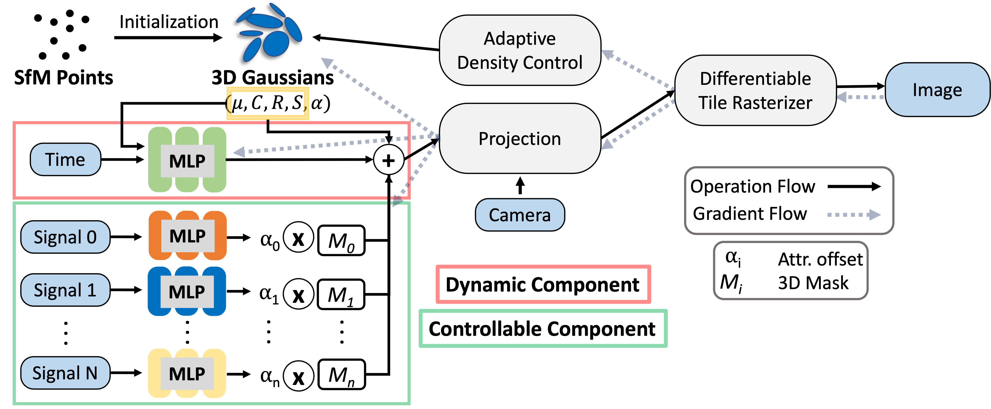
Figure 2: CoGS Overview. CoGS consists of two parts: Dynamic GS and Controllable GS.

3 Methods

In order to realize controllable GS, it is essential to first establish a GS framework capable of modeling dynamic scenes. This chapter is dedicated to unfolding this process in two distinct phases: initially, we introduce the concept and methodology of dynamic GS. Subsequently, we build upon this foundation to evolve these methods into a controllable framework, thereby enhancing their adaptability and applicability in dynamic scene modeling.

3.1 Dynamic Gaussian Splatting

To represent dynamic scenes and ultimately introduce fine-scale attribute control with 3D Gaussians, we utilize the differentiable Gaussian rasterization pipeline proposed by [14]. In specific, we directly follow the method therein and then augment its static properties with deformation fields to model scene dynamics.

3.1.1 Differentiable Rasterization of 3D Gaussians

Each 3D Gaussian is defined by a full 3D covariance matrix $\mathbf{\Sigma}$, position (mean) $\mathbf{\mu}$, opacity $\alpha$, and color represented via spherical harmonics (SH). To render these 3D Gaussians, projecting them from 3D to 2D Gaussians, we follow the procedure outlined in [48] to obtain the view space covariance matrix $\mathbf{\Sigma^{\prime}}$:

$$\mathbf{\Sigma^{\prime}}=\mathbf{J}\mathbf{W}\mathbf{\Sigma}\mathbf{W}^{T}\mathbf{J}^{T},$$ (1)

where $\mathbf{W}$ is the view transform and $\mathbf{J}$ is the Jacobian of the affine approximation of the projective transformation.

Since the physical meaning of a covariance matrix is only valid if it is positive semi-definite, it cannot be easily optimized to best represent a scene’s radiance field [14]. However, we can obscure this complexity by employing a parameterization that inherently maintains the positive semi-definiteness of the matrix. The covariance matrix $\Sigma$ can be decomposed into intuitive and optimizable components that correspond to an ellipsoid’s scaling and orientation with rotation matrix $\mathbf{R}$ and scaling matrix $\mathbf{S}$:

$$\mathbf{\Sigma}=\mathbf{R}\mathbf{S}\mathbf{S}^{T}\mathbf{R}^{T}.$$ (2)

and optimize $\mathbf{R}$, $\mathbf{S}$ instead of $\mathbf{\Sigma}$. After projection, the Gaussians are sorted from front-to-back where the color $C$ is given by NeRF-like volumetric rendering along a ray:

$$\mathbf{C}=\sum^{N}_{i=1}T_{i}(1-exp(-\sigma_{i}\delta_{i}))\mathbf{c}_{i},$$ (3)

with:

$$T_{i}=exp(-\sum_{j=1}^{i-1}\sigma_{j}\delta_{j}).$$ (4)

During optimization, we adaptively control the density of the 3D Gaussians to best represent the scene. Throughout this process, the total number of Gaussians will change. For a more comprehensive outline of this procedure, we kindly ask the readers to refer to [14].

3.1.2 Optimization for Dynamic Scene Representation

The defining parameters of each 3D Gaussian presuppose a static scene. Our approach bridges this gap to dynamic scenarios by learning independent deformation networks for each parameter. Additionally, we introduce multiple losses to maintain geometric consistency across time. The pipeline overview is presented in Fig. 2, with the dynamic component highlighted in red.

We initialize a set of 3D Gaussians from a Structure from Motion (SfM) [33] point-cloud (or randomly selecting $N$ points within the scene box), each defined by the same parameters as in 3.1.1. For the first 3000 iterations, our focus is exclusively on learning the static elements within the scene. This deliberate emphasis on stabilizing the static portions proves to be crucial for achieving high performance on the dynamic reconstruction. Establishing a robust static foundation lays the groundwork for a more accurate reconstruction of dynamic elements. During this phase, the deformation network (green MLP) does not update any parameters. Instead, these 3D Gaussians adhere to the same differentiable rasterization pipeline as covered in Section 3.1.1.

In the subsequent phases, the deformation network is employed to update each parameter, tailoring them to the dynamic scene. Although not explicitly depicted in Fig. 2, we learn $j$ separate networks, one for each parameter. For ($\mathbf{\mu_{i}}$, $\mathbf{C}_{i}$, $\mathbf{R_{i}}$, $\mathbf{S_{i}}$), we have a network $N_{j}$ such that:

$$N_{j}(\mathbf{\mu_{i}},t)=(\Delta\mathbf{\mu_{i}},\Delta\mathbf{C}_{i},\Delta\mathbf{R_{i}},\Delta\mathbf{S_{i}}),$$ (5)

where $t$ is the current time step. Different from [42], we also learn an offset for color to account for any changes that may occur over time (e.g. shadows and reflections). The output from these networks is then added to the corresponding parameters, and the differentiable rasterization pipeline proceeds.

Learning offsets alone results in a method that is unaware of consistent trajectories and accurate movement. Thus, we employ our multiple regularization losses to further constrain this difficult problem.

For each time step, the mean of the normalized predicted position offsets ($\Delta\mathbf{\mu}$) is computed to ensure their consistency with one another. Specifically, we use this to localize position offsets.

$$\mathcal{L}^{\text{norm}}=\frac{1}{N}\sum^{N}_{i=1}\|\Delta\mathbf{\mu_{i}}\|.$$ (6)

As shown in Fig. 3, the trajectories of static portions of the scene tend to stabilize with the addition of this loss.

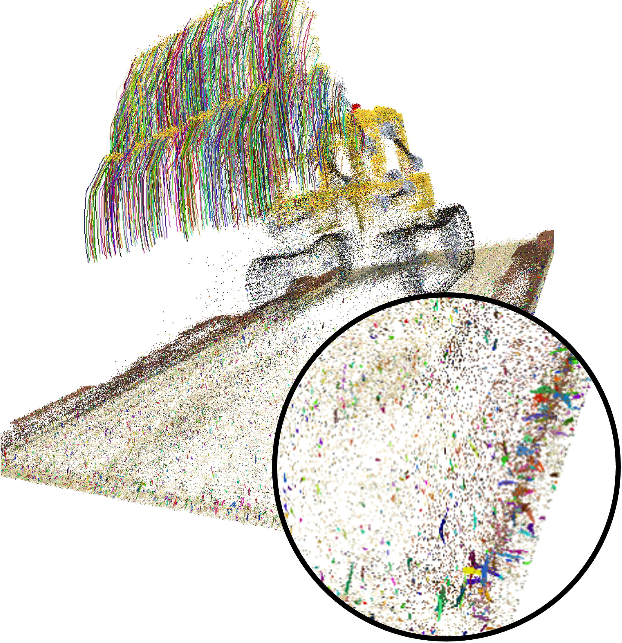
(a)

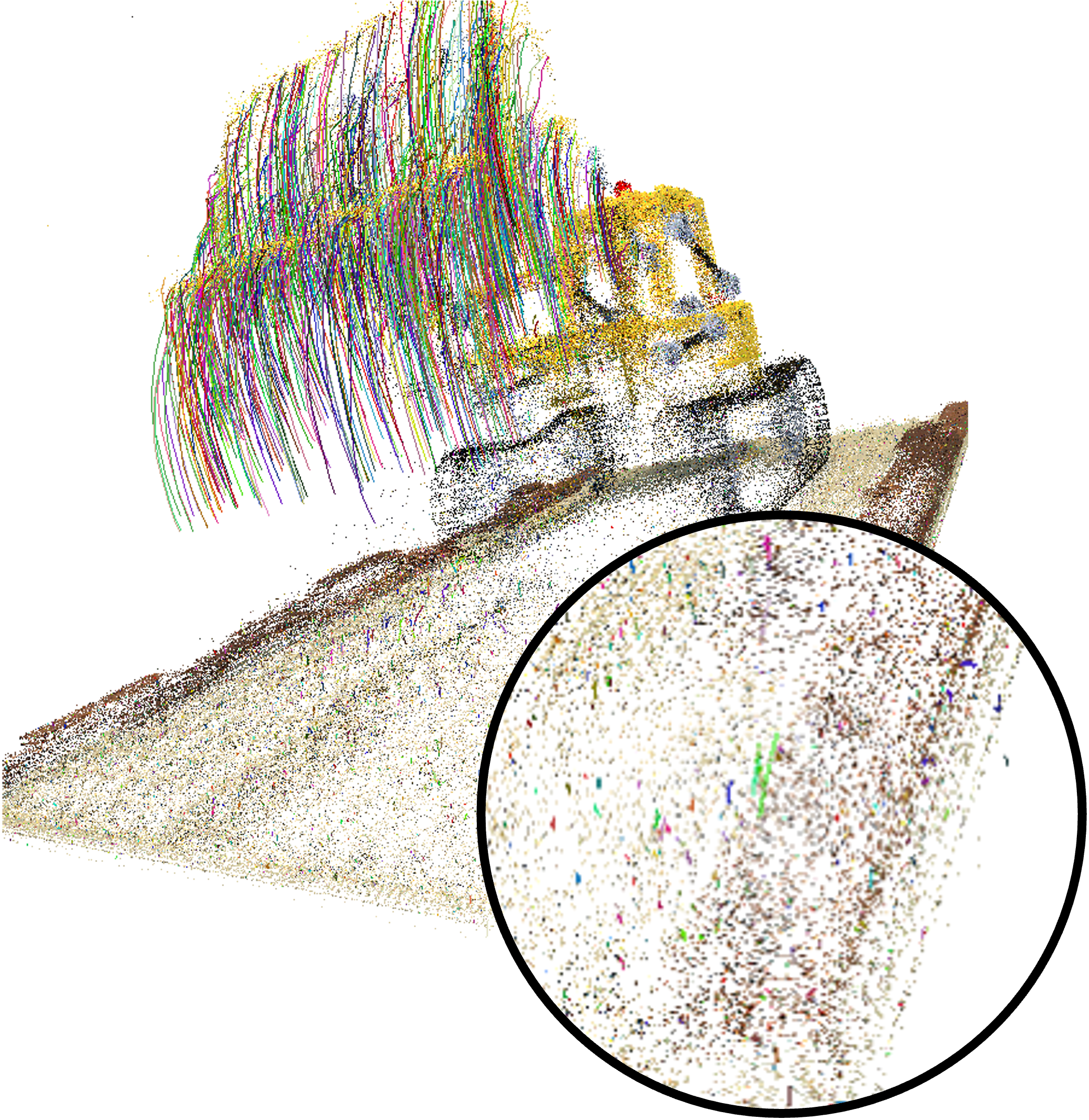
(b)

Figure 3: Lego synthetic scene visualized as a pointcloud of colored Gaussian centers. The smaller and fewer colored lines indicate less change in position over time. Adding $\mathcal{L^{\text{norm}}}$ stabilizes the static Gaussian’s positions. (a) Without $\mathcal{L^{\text{norm}}}$. (b) With $\mathcal{L^{\text{norm}}}$.

After 15000 iterations, we enforce the remainder of our losses. Specifically, a local difference loss, denoted as $\mathcal{L}^{\text{diff}}$, is used to ensure the movement, or trajectory, for each Gaussian is consistent with its neighbors over time. This loss is formulated as follows:

$$\mathcal{L}^{\text{diff}}_{i,j}=\left|\|\mathbf{\mu}_{i,j,t}-\mathbf{\mu_{i,t}}\|-\|\mathbf{\mu_{i,j,t-1}}-\mathbf{\mu_{i,t-1}}\|\right|.$$ (7)

Here, $\mu_{i,j,t}$ represents the position of a nearest neighbor Gaussian $j$ to Gaussian $i$ at time $t$. Similarly, $\mu_{i,t}$ is the position of Gaussian $i$ at time $t$, and analogous notation is used for the time step $t-1$.

The overall local difference loss is then defined as the average over all Gaussians $i$ and their $k$-nearest neighbours:

$$\mathcal{L}^{\text{diff}}=\frac{1}{k|G|}\sum_{i\in G}\sum_{j\in\text{knn}_{i;k}}\mathcal{L}^{\text{diff}}_{i,j}.$$ (8)

Demonstrated in Fig. 4(a), this loss yields a much more consistent dynamic representation when compared to without it as shown in 4(b).

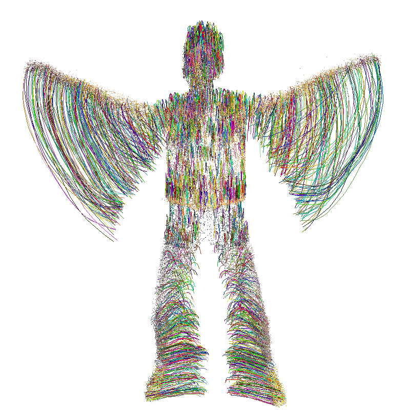
(a)

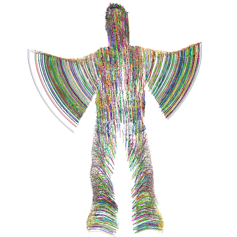
(b)

Figure 4: Jumping Jack synthetic scene visualized as a pointcloud of colored Gaussian centers. The smaller and fewer colored lines indicate less change in position over time. Adding $\mathcal{L^{\text{diff}}}$ stabilizes the 3D Gaussian’s trajectories. (a) Without $\mathcal{L^{\text{diff}}}$. (b) With $\mathcal{L^{\text{diff}}}$.

The next two loss functions are directly taken from [22], for more in depth details, please refer to their paper. Each of these losses are assigned a weight through an unnormalized Gaussian weighting factor:

$$w_{i,j}=\exp{(-\lambda_{w}\|\mu_{j,0}-\mu_{i,0}\|^{2}_{2})}$$ (9)

The distance between each Gaussian’s position is computed at the first time step, and then it is fixed for the remaining part of the sequence. In doing this, each of the following losses are explicitly locally enforced.

Using this weighting scheme, a local-rigidity loss is employed, denoted as $\mathcal{L}^{\text{rigid}}$, defined as follows:

$$\mathcal{L}^{\text{rigid}}_{i,j}=w_{i,j}||(\mu_{j,t-1}-\mu_{i,t-1})-\mathbf{R}_{i,t-1}\mathbf{R}^{-1}_{i,t}(\mu_{j,t}-\mu_{i,t}||_{2},$$ (10)

$$\mathcal{L}^{\text{rigid}}=\frac{1}{k|G|}\sum_{i\in G}\sum_{j\in\text{knn}_{i;k}}\mathcal{L}^{\text{rigid}}_{i,j}.$$ (11)

This loss ensures that for each Gaussian $i$, neighboring Gaussians $j$ should move in a manner consistent with the rigid body transform of the coordinate system over time.

Additionally, we incorporate a rotational loss $\mathcal{L}^{\text{rot}}$ to maintain consistency in rotations among nearby Gaussians across different time steps. This is expressed as:

$$\mathcal{L}^{\text{rot}}=\frac{1}{k|G|}\sum_{i\in G}\sum_{j\in\text{knn}_{i;k}}w_{i,j}\|\hat{q}_{j,t}\hat{q}_{j,t-1}^{-1}-\hat{q}_{i,t}\hat{q}_{i,t-1}^{-1}\|_{2},$$ (12)

where $\hat{q}$ is the normalized quaternion rotation of each Gaussian. The same $k$-nearest neighbors are used, as in the preceding losses.

Each of the described losses is critical to success at dynamic scene reconstruction, as there exist multiple facets that require precise constraints.

3.2 Controllable Gaussian Splatting

Having established the framework for dynamic GS, we can now extend it to accommodate controllable scenarios as shown in Fig. 2. This extension is facilitated by its explicit, Gaussian-based representation. The comprehensive pipeline of our approach comprises four key steps:

1. Building a Dynamic GS Model: As previously discussed, this foundational step establishes the groundwork for subsequent extensions.

2. 3D Mask Generation: This step involves translating two-dimensional mask data into a three-dimensional context, bridging the gap between simple representations and complex spatial models. The 2D mask is either annotated manually quite easily or automatically inferred by existing methods.

3. Control Signal Extraction: A pivotal phase where control signals are identified and extracted manually or automatically from explict Gaussian sets, serving as the primary drivers for scene manipulation.

4. Control Signal Re-Alignment: The final phase, which entails adjusting and aligning the control signals to ensure their seamless integration and responsiveness within the dynamic model.

In the following sections, we will explore the details of the last three steps, elucidating their roles in enhancing the overall efficacy and controllability of our dynamic GS.

3.2.1 3D Mask Generation

To delineate the controllable set of Gaussians, we introduce a mask vector $m_{i}\in\mathbb{R}^{L}$ for each Gaussian, where $L$ denotes the number of attributes to be controlled. The straightforward approach of selecting these in 3D introduces two major challenges: the complexity of manually labeling Gaussian positions for each attribute and the difficulty in achieving an exact fine-grained boundary for the 3D point set, potentially leading to control artifacts.

Addressing these challenges, we propose an effective method to obtain the mask vector $m$. We start by acquiring $K$ 2D masks for the 2D frames, where $K$ can vary from all frames (for scenarios with available automatic mask generation methods like face recognition [45], as illustrated in Fig. 7(d)) to a single frame (which can be manually labeled, as demonstrated in Figs. 7(a) & 7(b) & 7(c)). After the 2D mask acquisition, we perform a 2D-to-3D mask projection. A practical method involves associating the 3D point with the corresponding 2D pixel, utilizing depth maps and camera poses as in [22]. However, this method falls short of attaining the fine-grained boundary of the controllable part due to the splatting process 3.1.1.

Therefore, we suggest a learning process to obtain the mask vector for each Gaussian. We allocate a learnable mask tensor $m_{i}\in\mathbb{R}^{L}$ to each Gaussian and implement a softmax operation to normalize the sum of the tensor to 1, aiming for a categorical distribution. For rendering the 2D mask $M$ from the 3D $m_{i}$, we use the same GS equation, referred to as Eq. 3, employing the same point $\mu$, rotation matrix $R$, and scaling matrix $S$, except that we set the color for each Gaussian as a constant (1), and take the mask tensor as opacity. This rendered 2D mask is supervised using the ground-truth mask. Importantly, rather than enforcing an exact match between the rendered and ground-truth masks for each control area, we focus on ensuring that the rendered mask has no impact (is black) on other control areas as in Eq. 13, significantly reducing artifacts at the boundaries. $M_{i}$ is the rendering 2D mask for the $i$th attribute and $M^{gt}_{i}$ is the corresponding ground truth. Here we want the rendering mask $M_{i}$ to ideally be black on other controllable areas so as to make no effect on these parts.

$$\mathcal{L}^{\text{mask}}=\sum^{L}_{i=1}\|(1-M_{i})-\sum^{L}_{j=1,j\neq i}M^{gt}_{j}\|\cdot\sum^{L}_{j=1,j\neq i}M^{gt}_{j}.$$ (13)

In this step, we maintain all other learnable weights and tensors, except for the mask tensor, as fixed.

3.2.2 Control Signal Extraction

Our method uniquely eliminates the need for pre-computed control signals, significantly expanding its range of applications. This is accomplished by unsupervised learning of the control signal directly from the Gaussians. The first step involves selecting a set of Gaussians, denoted as $G$, which represents movement within the control part, as indicated by the previously learned mask $m$. This set $G$ can be either manually selected in 3D or automatically based on movement trajectories, such as by choosing the set of points $\mathbf{p}$ with the largest movement distance. The size of this Gaussian set $G$ can be as minimal as a single Gaussian.

Utilizing the explicit representation of GS, we calculate the centroid $\mathbf{c}$ of the points in $G$ and trace its movement trajectory. We employ a simple linear model for trajectory analysis, although more complex models are feasible. Principal Component Analysis (PCA) is applied to determine the primary movement direction, denoted as $\mathbf{d}$. The positions of the Gaussian (means) $\mu$ are then projected onto this direction $\mathbf{d}$ at each timestep $t$, as shown in Eq. 14:

$$\mathbf{proj}_{\mathbf{d}}(\mu_{t})=\frac{(\mu_{t}-\mathbf{c})\cdot\mathbf{d}}{\|\mathbf{d}\|}.$$ (14)

This projection enables us to define the start and end points, $\mathbf{s}$ and $\mathbf{e}$, along the movement direction. Subsequently, the distances of all points from the start point $\mathbf{s}$ are normalized to a range between 0 and 1, resulting in our control signal $\sigma$, as expressed in Eq. 15:

$$\sigma(\mu_{t})=\frac{\mathbf{proj}_{\mathbf{d}}(\mu_{t})-\mathbf{proj}_{\mathbf{d}}(\mathbf{s})}{\mathbf{proj}_{\mathbf{d}}(\mathbf{e})-\mathbf{proj}_{\mathbf{d}}(\mathbf{s})}.$$ (15)

This process culminates in the control signal $\sigma$, enabling dynamic scene manipulation.

3.2.3 Control Signal Re-Alignment

After obtaining the control signal $\sigma$, the next crucial step is its integration into the network to facilitate manipulation using these signals. This is accomplished by developing a unique network $N^{c}_{i}$ for each control signal, designed to output the corresponding offset $\Delta$ for each Gaussian attribute, as determined in the dynamic modeling stage. Let $\mu_{i}$, $\mathbf{C}_{i}$, $\mathbf{R}_{i}$, and $\mathbf{S}_{i}$ denote the mean, rotation, and scaling of each Gaussian, respectively. The control network $N^{c}_{i}$ modifies these attributes in response to the control signal:

$$N^{c}_{i}(\sigma)=(\Delta\mu_{i},\Delta\mathbf{C}_{i},\Delta\mathbf{R_{i}},\Delta\mathbf{S_{i}})$$ (16)

In this phase, the focus is solely on training these control signal networks $N_{i}$, while keeping all other learnable parameters $\Theta$ fixed.

Upon achieving reliable estimates for the attribute offsets $\Delta\mu_{i},\Delta\mathbf{C}_{i},\Delta\mathbf{R_{i}},\Delta\mathbf{S_{i}}$ of each Gaussian, we move towards the end-to-end fine-tuning of all learnable parameters. This all-encompassing fine-tuning is crucial for completing our controllable GS model. The final model (represented by $f$) is formulated as:

$$f(\Theta;\mu_{i}+\Delta\mu_{i},\mathbf{C}_{i}+\Delta\mathbf{C}_{i},\mathbf{R_{i}}+\Delta\mathbf{R_{i}},\mathbf{S_{i}}+\Delta\mathbf{S_{i}})$$ (17)

This final step guarantees precise and effective control over dynamic scene renderings.

4 Experiments

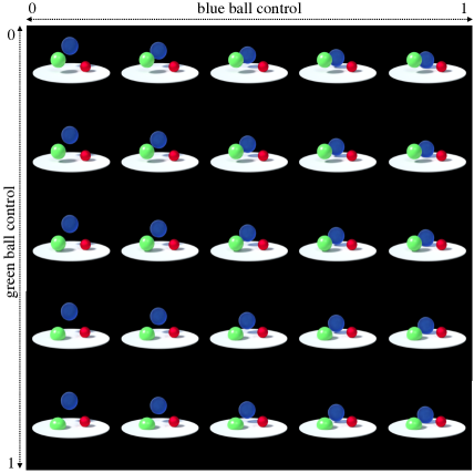
Figure 5: Control blue ball and green ball separately.

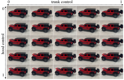
Figure 6: Opening the hood and the trunk of the toy car.

In this section, we present the experiments conducted to demonstrate the effectiveness of our method in dynamic and controllable scenarios.

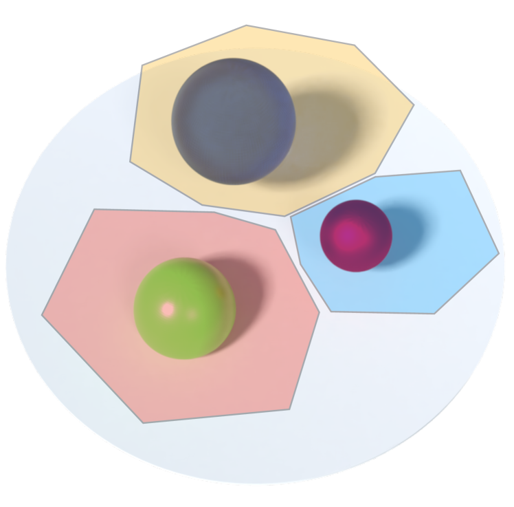
(a)

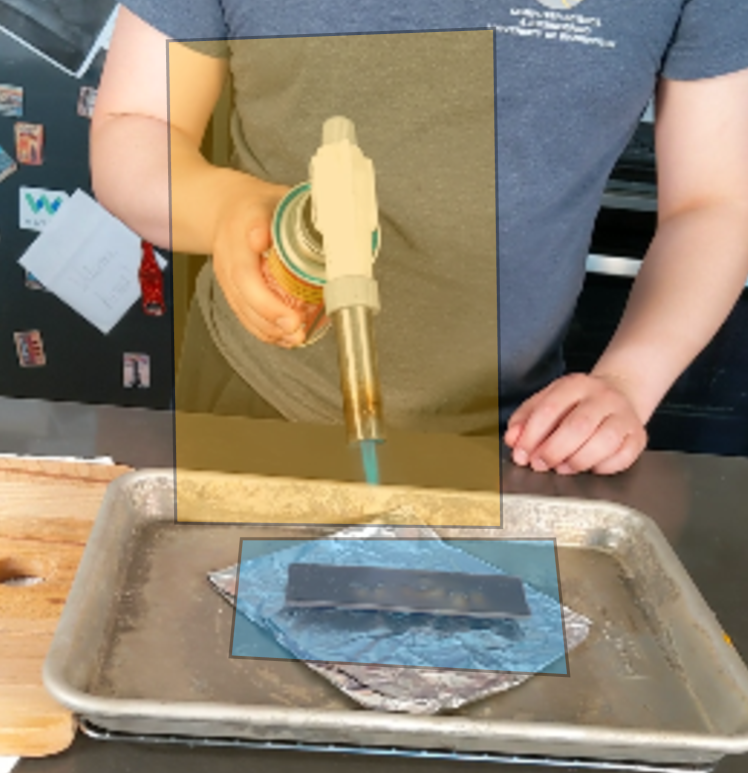
(b)

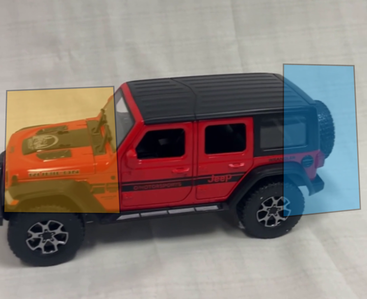
(c)

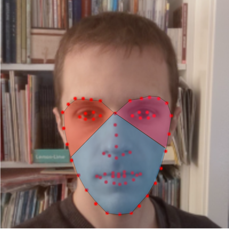
(d)

Figure 7: 2D mask labeling. (a)-(c) Manually labeling a single frame. (d) Automatic labeling using facial key-point detection.

Table 1: Quantitative results on synthetic dynamic scenes. We color code each row as best, second best, and third best.

Method	PSNR$\uparrow$	SSIM$\uparrow$	LPIPS$\downarrow$ (100x)
NeRF[24]	18.98	0.870	18.25
DirectVoxGo[34]	18.64	0.853	16.88
Plenoxels[8]	20.24	0.868	16.00
T-NeRF[32]	29.50	0.951	7.88
D-NeRF[32]	30.44	0.952	6.63
TiNeuVox-S[7]	30.75	0.955	6.63
TiNeuVox-B[7]	32.67	0.972	4.25
3D GS [14]	23.07	0.928	8.22
Ours	37.90	0.983	1.74
Ours, w/o $\mathcal{L}^{\text{norm}}$	37.41	0.984	1.70
Ours, w/o $\mathcal{L}^{\text{diff}}$	37.68	0.982	1.65
Ours, w/o $\mathcal{L}^{\text{rigid}}$	37.75	0.981	1.71

Table 2: Quantitative results on real dynamic scenes. We color code each row as best, second best, and third best.

Method	PSNR$\uparrow$	SSIM$\uparrow$	LPIPS$\downarrow$ (100x)
NeRF[24]	22.3	0.807	43.3
NV[21]	26.3	0.910	20.9
NSFF[19]	25.7	0.881	24.8
Nerfies[29]	29.3	0.948	17.6
HyperNeRF[30]	29.8	0.954	17.2
TiNeuVox-S[7]	23.6	0.690	54.5
TiNeuVox-B[7]	28.0	0.752	45.1
3D GS [14]	22.1	0.724	43.8
Ours	29.6	0.950	17.1
Ours, w/o $\mathcal{L}^{\text{norm}}$	29.1	0.905	20.1
Ours, w/o $\mathcal{L}^{\text{diff}}$	29.8	0.912	19.8
Ours, w/o $\mathcal{L}^{\text{rigid}}$	29.4	0.920	21.3

4.1 Datasets

To evaluate our dynamic model, experiments were conducted on two categories of dynamic scenes: synthetic and real. Additionally, the performance of our controllable model was assessed on a synthetic scene, real face scene, real dynamic scene, and a self-captured toy car scene.
Synthetic Scenes. We employed the $360^{\circ}$ dynamic synthetic dataset introduced by [32], comprising 8 animated objects with complex geometries and non-Lambertian materials. Each scene in this dataset includes $50$ to $200$ training images and $20$ test images, all at an $800\times 800$ resolution.
Real Scenes. Four topologically diverse scenes from [30] (torchocolate, cut-lemon, chickchicken, and hand) were used. These scenes were captured using a rig consisting of two Google Pixel 3 phones mounted approximately 16cm apart on a pole.
Real Face Scene. For controllable model testing, we utilized a real face scene from [13] (involving actions like closing/opening the eyes/mouth). This scene was captured with either a Google Pixel 3a or an Apple iPhone 13 Pro. Unlike CoNeRF, which requires pre-defined control signals and masks, our method achieves comparable controllability without such prerequisites.
Toy Car Scene. We also ran experiments on a self-captured Toy Car scene. The capture process involved manually opening the car’s trunk and hood separately, recording one video per transition. Once the transitions were completed, we stitched the individual videos together to create a single cohesive dynamic scene. This scene was captured with an Apple iPhone 13 Pro.

Jumping Jacks

(a) Ground Truth

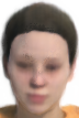
(b) D-NeRF [32]

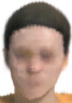
(c) TiNeuVox [7]

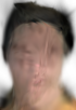
(d) 3D-GS [14]

(e) Ours

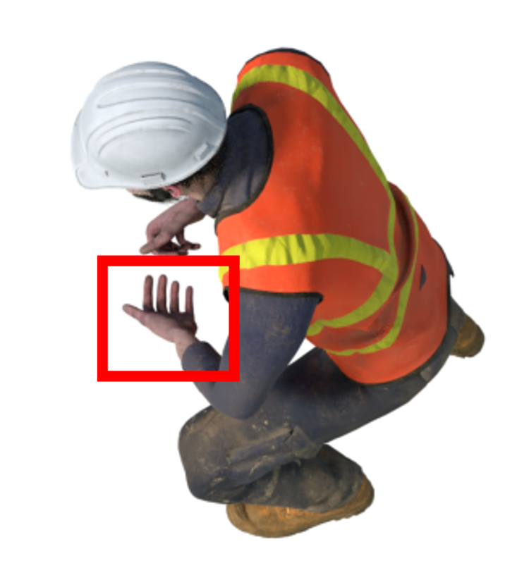
Standup

(f) Ground Truth

(g) D-NeRF [32]

(h) TiNeuVox [7]

(i) 3D-GS [14]

(j) Ours

Figure 8: Qualitative results on synthetic dynamic scenes. We compare our Dynamic 3D-GS method (Ours) with the ground truth, D-NeRF, TiNeuVox, and the static 3D-GS method.

Cut Lemon

(a) Ground Truth

(b) HyperNeRF [30]

(c) TiNeuVox [7]

(d) 3D-GS [14]

(e) Ours

Chick Chicken

(f) Ground Truth

(g) HyperNeRF [30]

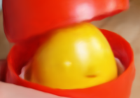
(h) TiNeuVox [7]

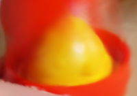
(i) 3D-GS [14]

(j) Ours

Figure 9: Qualitative results on real dynamic scenes. We compare our Dynamic 3D-GS method (Ours) with the ground truth, HyperNeRF, TiNeuVox, and the static 3D-GS method. For Cut Lemon, our method models the knuckles on the hand better than others. As for Chick Chicken, we reconstruct more fine details (red edges).

4.2 Implementation Details

For the training of the dynamic component, we adopted the differential Gaussian rasterization technique from 3D GS [14], and implemented the additional network components using PyTorch [31]. The Gaussians were initialized either using SfM results or by randomly selecting $N$ points (where $N=10k$ in our experiments) within the scene box. The initial phase of 3k iterations does not involve learning any deformation field; this phase is akin to the training process of 3D GS, aiding in the convergence of the learning process. Following this, we jointly train the 3D Gaussian attributes and the deformation network for a total of 50k iterations. The learning rate for each Gaussian attribute is kept consistent with that used in 3D GS, as detailed in [14], while the learning rate for the deformation network is set to exponentially decay from $1e-3$ to $1e-6$.

In the controllable part, the learning rate is set to 1 for the initial 1k iterations during the 3D Mask Generation phase. During the Control Signal Re-Alignment phase, we apply an exponential decay of the learning rate from $1e-2$ to $1e-4$ over 5k iterations, specifically for training the control signal networks. For the final end-to-end finetuning, the learning rate is set to $1e-6$, and the process is run for an additional 5k iterations. Optimization throughout these processes is performed using the Adam optimizer [15] with a $\beta$ value range of $(0.9,0.999)$. All experiments were conducted using single 80GB NVIDIA A100 GPUs.

4.3 Results

We show the qualitative and quantitative results in this section to demonstrate the effectiveness of our method. We use Peak Signal-to-Noise Ratio (PSNR) [12] in decibels (dB), the Structural Similarity Index (SSIM) [40, 28] and the Learned Perceptual Image Patch Similarity (LPIPS) [47] as evaluation metrics. All detailed results for each scene can be found in the supplementary material.

We first show our dynamic GS modeling part. We compare our method with existing works using dynamic synthetic scenes from [32] on the novel view synthesis task. We report the quantitative results in Table 1 and we can see that our method can achieve much better performance than existing methods. The qualitative results are shown in Fig. 9 and we can see that our method has better face and hand details. For the real scenes from [30], we run interpolation experiments as in [30] instead of the novel view synthesis task because of the rendering pose problem mentioned in [42]. We show our results in Table 2 and Fig. 9. We can see that our method can capture better details on complex real dynamic scenes. We also perform ablation experiments on the regularizations we utilize as shown in Table 1 & 2. To better illustrate the role of the regularizations, we also visualize the trajectories in Fig. 4.

For the controllable GS, we use four datasets (bouncingball, torchocolate, face and car) and first fit a dynamic GS on them. Then we obtain the labels as shown in Fig. 7. For the eye scene, we manually select the point set as the control points, and for other scenes, we get the point sets automatically from the point movement as mentioned before. We also visualize the control results to demonstrate our method’s performance.

Table 3: Quantitative results on controllable face scenes. We color code each row as best, second best, and third best.

Method	PSNR$\uparrow$	SSIM$\uparrow$	LPIPS$\downarrow$ (100x)
NeRF [24]	28.80	0.951	21.0
NeRF + Latent [24]	32.65	0.981	18.2
Nerfies[29]	32.27	0.981	18.0
HyperNeRF[30]	32.52	0.981	16.9
CoNeRF-$M$[13]	32.06	0.979	16.7
CoNeRF[13]	32.34	0.981	16.8
3D GS [14]	25.94	0.834	41.4
Ours	32.60	0.983	16.4

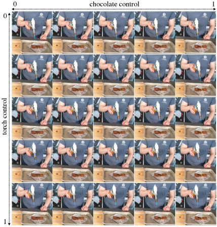
Figure 10: Controlling the blowtorch and the melting chocolate separately.

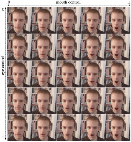
Figure 11: Controlling the eyes and the mouth separately.

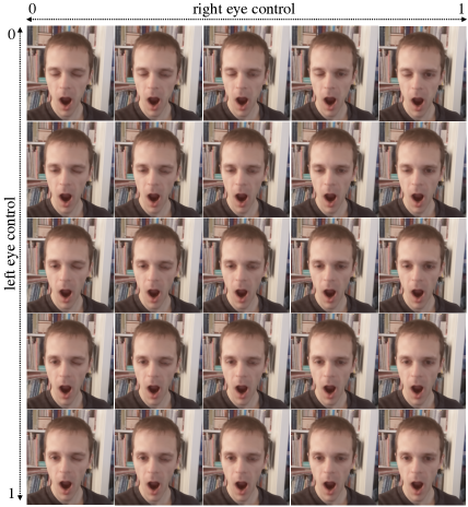
Figure 12: Controlling the left eye and right eye separately.

5 Conclusion

We presented Controllable Gaussian Splatting named CoGS, a novel method for dynamic scene manipulation. It overcomes the limitations of NeRFs and similar neural methods by using an explicit representation that enables real-time, controllable manipulation of dynamic scenes. Our approach, validated through extensive experiments, shows superior performance in visual fidelity and manipulation capabilities compared to existing techniques. The explicit nature of CoGS not only enhances efficiency in rendering but also simplifies scene element manipulation. It has the potential to democratize 3D deformable content creation using commodity hardware, making it more accessible and feasible for a broader range of users and applications.

References

- Athar et al. [2022] ShahRukh Athar, Zexiang Xu, Kalyan Sunkavalli, Eli Shechtman, and Zhixin Shu. Rignerf: Fully controllable neural 3d portraits. In Proceedings of the IEEE/CVF conference on Computer Vision and Pattern Recognition, pages 20364–20373, 2022.
- Barron et al. [2021] Jonathan T Barron, Ben Mildenhall, Matthew Tancik, Peter Hedman, Ricardo Martin-Brualla, et al. Mip-NeRF: A Multiscale Representation for Anti-Aliasing Neural Radiance Fields. In Proc. IEEE/CVF ICCV, pages 5855–5864, 2021.
- Cao et al. [2023] Junli Cao, Huan Wang, Pavlo Chemerys, Vladislav Shakhrai, Ju Hu, Yun Fu, Denys Makoviichuk, Sergey Tulyakov, and Jian Ren. Real-time neural light field on mobile devices. In Proceedings of the IEEE/CVF Conference on Computer Vision and Pattern Recognition, pages 8328–8337, 2023.
- Chen et al. [2022] Anpei Chen, Zexiang Xu, Andreas Geiger, Jingyi Yu, and Hao Su. Tensorf: Tensorial radiance fields. In European Conference on Computer Vision, pages 333–350. Springer, 2022.
- Deng et al. [2022] Kangle Deng, Andrew Liu, Jun-Yan Zhu, and Deva Ramanan. Depth-supervised NeRF: Fewer Views and Faster Training for Free. In Proc. IEEE/CVF CVPR, pages 12882–12891, 2022.
- Du et al. [2021] Yilun Du, Yinan Zhang, Hong-Xing Yu, Joshua B Tenenbaum, and Jiajun Wu. Neural radiance flow for 4d view synthesis and video processing. In 2021 IEEE/CVF International Conference on Computer Vision (ICCV), pages 14304–14314. IEEE Computer Society, 2021.
- Fang et al. [2022] Jiemin Fang, Taoran Yi, Xinggang Wang, Lingxi Xie, Xiaopeng Zhang, et al. Fast Dynamic Radiance Fields with Time-Aware Neural Voxels. arXiv:2205.15285, 2022.
- Fridovich-Keil et al. [2022] Sara Fridovich-Keil, Alex Yu, Matthew Tancik, Qinhong Chen, Benjamin Recht, et al. Plenoxels: Radiance Fields Without Neural Networks. In Proc. IEEE/CVF CVPR, pages 5501–5510, 2022.
- Gafni et al. [2021] Guy Gafni, Justus Thies, Michael Zollhofer, and Matthias Nießner. Dynamic Neural Radiance Fields for Monocular 4D Facial Avatar Reconstruction. In Proc. IEEE/CVF CVPR, pages 8649–8658, 2021.
- Gao et al. [2021] Chen Gao, Ayush Saraf, Johannes Kopf, and Jia-Bin Huang. Dynamic view synthesis from dynamic monocular video. In Proceedings of the IEEE/CVF International Conference on Computer Vision, pages 5712–5721, 2021.
- Garbin et al. [2022] Stephan J Garbin, Marek Kowalski, Virginia Estellers, Stanislaw Szymanowicz, Shideh Rezaeifar, Jingjing Shen, Matthew Johnson, and Julien Valentin. Voltemorph: Realtime, controllable and generalisable animation of volumetric representations. arXiv preprint arXiv:2208.00949, 2022.
- Hore and Ziou [2010] Alain Hore and Djemel Ziou. Image quality metrics: PSNR vs. SSIM. In 20th ICPR, pages 2366–2369. IEEE, 2010.
- Kania et al. [2022] Kacper Kania, Kwang Moo Yi, Marek Kowalski, Tomasz Trzciński, and Andrea Tagliasacchi. CoNeRF: Controllable Neural Radiance Fields. In Proc. IEEE/CVF CVPR, pages 18623–18632, 2022.
- Kerbl et al. [2023] Bernhard Kerbl, Georgios Kopanas, Thomas Leimkühler, and George Drettakis. 3d gaussian splatting for real-time radiance field rendering. ACM Transactions on Graphics (ToG), 42(4):1–14, 2023.
- Kingma and Ba [2014] Diederik P Kingma and Jimmy Ba. Adam: A Method for Stochastic Optimization. arXiv:1412.6980, 2014.
- Lazova et al. [2023] Verica Lazova, Vladimir Guzov, Kyle Olszewski, Sergey Tulyakov, and Gerard Pons-Moll. Control-nerf: Editable feature volumes for scene rendering and manipulation. In Proceedings of the IEEE/CVF Winter Conference on Applications of Computer Vision, pages 4340–4350, 2023.
- Li et al. [2022a] Lingzhi Li, Zhen Shen, Zhongshu Wang, Li Shen, and Ping Tan. Streaming radiance fields for 3d video synthesis. Advances in Neural Information Processing Systems, 35:13485–13498, 2022a.
- Li et al. [2022b] Tianye Li, Mira Slavcheva, Michael Zollhoefer, Simon Green, Christoph Lassner, Changil Kim, Tanner Schmidt, Steven Lovegrove, Michael Goesele, Richard Newcombe, et al. Neural 3d video synthesis from multi-view video. In Proceedings of the IEEE/CVF Conference on Computer Vision and Pattern Recognition, pages 5521–5531, 2022b.
- Li et al. [2021] Zhengqi Li, Simon Niklaus, Noah Snavely, and Oliver Wang. Neural scene flow fields for space-time view synthesis of dynamic scenes. In Proceedings of the IEEE/CVF Conference on Computer Vision and Pattern Recognition, pages 6498–6508, 2021.
- Lin et al. [2022] Haotong Lin, Sida Peng, Zhen Xu, Yunzhi Yan, Qing Shuai, Hujun Bao, and Xiaowei Zhou. Efficient neural radiance fields for interactive free-viewpoint video. In SIGGRAPH Asia 2022 Conference Papers, pages 1–9, 2022.
- Lombardi et al. [2019] Stephen Lombardi, Tomas Simon, Jason Saragih, Gabriel Schwartz, Andreas Lehrmann, and Yaser Sheikh. Neural volumes: learning dynamic renderable volumes from images. ACM Transactions on Graphics (TOG), 38(4):1–14, 2019.
- Luiten et al. [2023] Jonathon Luiten, Georgios Kopanas, Bastian Leibe, and Deva Ramanan. Dynamic 3d gaussians: Tracking by persistent dynamic view synthesis. arXiv preprint arXiv:2308.09713, 2023.
- Martin-Brualla et al. [2021] Ricardo Martin-Brualla, Noha Radwan, Mehdi SM Sajjadi, Jonathan T Barron, Alexey Dosovitskiy, et al. NeRF in the Wild: Neural Radiance Fields for Unconstrained Photo Collections. In Proc. IEEE/CVF CVPR, pages 7210–7219, 2021.
- Mildenhall et al. [2021] Ben Mildenhall, Pratul P Srinivasan, Matthew Tancik, Jonathan T Barron, Ravi Ramamoorthi, et al. NeRF: Representing Scenes as Neural Radiance Fields for View Synthesis. Commun. ACM, 65(1):99–106, 2021.
- Mildenhall et al. [2022] Ben Mildenhall, Peter Hedman, Ricardo Martin-Brualla, Pratul P Srinivasan, and Jonathan T Barron. NeRF in the Dark: High Dynamic Range View Synthesis from Noisy Raw Images. In Proc. IEEE/CVF CVPR, pages 16190–16199, 2022.
- Mubarik et al. [2023] Muhammad Husnain Mubarik, Ramakrishna Kanungo, Tobias Zirr, and Rakesh Kumar. Hardware acceleration of neural graphics. In Proceedings of the 50th Annual International Symposium on Computer Architecture, pages 1–12, 2023.
- Müller et al. [2022] Thomas Müller, Alex Evans, Christoph Schied, and Alexander Keller. Instant neural graphics primitives with a multiresolution hash encoding. ACM Transactions on Graphics (ToG), 41(4):1–15, 2022.
- Odena et al. [2017] Augustus Odena, Christopher Olah, and Jonathon Shlens. Conditional Image Synthesis with Auxiliary Classifier GANs. In ICML, pages 2642–2651. PMLR, 2017.
- Park et al. [2021a] Keunhong Park, Utkarsh Sinha, Jonathan T Barron, Sofien Bouaziz, Dan B Goldman, et al. Nerfies: Deformable Neural Radiance Fields. In Proc. IEEE/CVF ICCV, pages 5865–5874, 2021a.
- Park et al. [2021b] Keunhong Park, Utkarsh Sinha, Peter Hedman, Jonathan T Barron, Sofien Bouaziz, et al. HyperNeRF: A Higher-Dimensional Representation for Topologically Varying Neural Radiance Fields. ACM Trans. Graph., 40(6):1–12, 2021b.
- Paszke et al. [2019] Adam Paszke, Sam Gross, Francisco Massa, Adam Lerer, James Bradbury, Gregory Chanan, Trevor Killeen, Zeming Lin, Natalia Gimelshein, Luca Antiga, et al. Pytorch: An imperative style, high-performance deep learning library. Advances in neural information processing systems, 32, 2019.
- Pumarola et al. [2021] Albert Pumarola, Enric Corona, Gerard Pons-Moll, and Francesc Moreno-Noguer. D-NeRF: Neural Radiance Fields for Dynamic Scenes. In Proc. IEEE/CVF CVPR, pages 10318–10327, 2021.
- Schonberger and Frahm [2016] Johannes L Schonberger and Jan-Michael Frahm. Structure-from-motion revisited. In Proceedings of the IEEE conference on computer vision and pattern recognition, pages 4104–4113, 2016.
- Sun et al. [2022] Cheng Sun, Min Sun, and Hwann-Tzong Chen. Direct voxel grid optimization: Super-fast convergence for radiance fields reconstruction. In Proceedings of the IEEE/CVF Conference on Computer Vision and Pattern Recognition, pages 5459–5469, 2022.
- Tretschk et al. [2021] Edgar Tretschk, Ayush Tewari, Vladislav Golyanik, Michael Zollhöfer, Christoph Lassner, et al. Non-Rigid Neural Radiance Fields: Reconstruction and Novel View Synthesis of a Dynamic Scene From Monocular Video. In Proc. IEEE/CVF ICCV, pages 12959–12970, 2021.
- Wang et al. [2023a] Chaoyang Wang, Lachlan Ewen MacDonald, Laszlo A Jeni, and Simon Lucey. Flow supervision for deformable nerf. In Proceedings of the IEEE/CVF Conference on Computer Vision and Pattern Recognition, pages 21128–21137, 2023a.
- Wang et al. [2023b] Feng Wang, Sinan Tan, Xinghang Li, Zeyue Tian, Yafei Song, and Huaping Liu. Mixed neural voxels for fast multi-view video synthesis. In Proceedings of the IEEE/CVF International Conference on Computer Vision, pages 19706–19716, 2023b.
- Wang et al. [2022] Liao Wang, Jiakai Zhang, Xinhang Liu, Fuqiang Zhao, Yanshun Zhang, et al. Fourier PlenOctrees for Dynamic Radiance Field Rendering in Real-time. In Proc. IEEE/CVF CVPR, pages 13524–13534, 2022.
- Wang et al. [2021] Peng Wang, Lingjie Liu, Yuan Liu, Christian Theobalt, Taku Komura, et al. NeuS: Learning Neural Implicit Surfaces by Volume Rendering for Multi-view Reconstruction. Adv. NeurIPS, 34:27171–27183, 2021.
- Wang et al. [2004] Zhou Wang, Alan C Bovik, Hamid R Sheikh, and Eero P Simoncelli. Image Quality Assessment: From Error Visibility to Structural Similarity. IEEE Trans. Image Process., 13(4):600–612, 2004.
- Wu et al. [2023] Guanjun Wu, Taoran Yi, Jiemin Fang, Lingxi Xie, Xiaopeng Zhang, Wei Wei, Wenyu Liu, Qi Tian, and Xinggang Wang. 4d gaussian splatting for real-time dynamic scene rendering. arXiv preprint arXiv:2310.08528, 2023.
- Yang et al. [2023a] Ziyi Yang, Xinyu Gao, Wen Zhou, Shaohui Jiao, Yuqing Zhang, and Xiaogang Jin. Deformable 3d gaussians for high-fidelity monocular dynamic scene reconstruction. arXiv preprint arXiv:2309.13101, 2023a.
- Yang et al. [2023b] Zeyu Yang, Hongye Yang, Zijie Pan, Xiatian Zhu, and Li Zhang. Real-time photorealistic dynamic scene representation and rendering with 4d gaussian splatting. arXiv preprint arXiv:2310.10642, 2023b.
- Yariv et al. [2023] Lior Yariv, Peter Hedman, Christian Reiser, Dor Verbin, Pratul P Srinivasan, Richard Szeliski, Jonathan T Barron, and Ben Mildenhall. Bakedsdf: Meshing neural sdfs for real-time view synthesis. arXiv preprint arXiv:2302.14859, 2023.
- Yu et al. [2023a] Heng Yu, Joel Julin, Zoltan A Milacski, Koichiro Niinuma, and László A Jeni. Dylin: Making light field networks dynamic. In Proceedings of the IEEE/CVF Conference on Computer Vision and Pattern Recognition, pages 12397–12406, 2023a.
- Yu et al. [2023b] Heng Yu, Koichiro Niinuma, and László A Jeni. Confies: Controllable neural face avatars. In 2023 IEEE 17th International Conference on Automatic Face and Gesture Recognition (FG), pages 1–8. IEEE, 2023b.
- Zhang et al. [2018] Richard Zhang, Phillip Isola, Alexei A Efros, Eli Shechtman, and Oliver Wang. The Unreasonable Effectiveness of Deep Features as a Perceptual Metric. In Proc. IEEE/CVF CVPR, pages 586–595, 2018.
- Zwicker et al. [2001] M. Zwicker, H. Pfister, J. van Baar, and M. Gross. Ewa volume splatting. In Proceedings Visualization, 2001. VIS ’01., pages 29–538, 2001.