Set-valued recursions arising from vantage-point trees

Abstract.

We study vantage-point trees constructed using an independent sample from the uniform distribution on a fixed convex body $K$ in $(\mathbb{R}^{d},\|\cdot\|)$, where $\|\cdot\|$ is an arbitrary homogeneous norm on $\mathbb{R}^{d}$. We prove that a sequence of sets, associated with the left boundary of a vantage-point tree, forms a recurrent Harris chain on the space of convex bodies in $(\mathbb{R}^{d},\|\cdot\|)$. The limiting object is a ball polyhedron, that is, an a.s. finite intersection of closed balls in $(\mathbb{R}^{d},\|\cdot\|)$ of possibly different radii. As a consequence, we derive a limit theorem for the length of the leftmost path of a vantage-point tree.

1. Introduction

Let $(M,\rho)$ be a metric space. The notation $B_{r}(x)$ is used for the closed ball of radius $r$ centered at $x$, that is, $B_{r}(x):=\{y\in M:\rho(x,y)\leq r\}$. A vantage-point tree (in short, vp tree) $\mathbb{VP}(\mathcal{X})$ of a (finite or infinite) sequence $\mathcal{X}:=(x_{1},x_{2},\ldots)\subset M$ with a threshold function $r$ is a labeled rooted subtree of a full binary tree constructed using the following rules.

• Each vertex of $\mathbb{VP}(\mathcal{X})$ is a pair $(x,r_{x})$, where $x\in\mathcal{X}$ is called a vantage-point and its label $r_{x}$ is a positive real number called the threshold of $x$.

• $\mathbb{VP}(x_{1})$ is the unique tree with a single vertex (the root) $(x_{1},r_{x_{1}})$, where $r_{x_{1}}$ is a given positive number, the threshold of the root.

• For a finite set $(x_{1},\dots,x_{k})\subset M$, the tree $\mathbb{VP}(x_{1},\dots,x_{k},x)$ is constructed by adding a new vertex $(x,r_{x})$ to $\mathbb{VP}(x_{1},\dots,x_{k})$ by recursively comparing $x$ with $x_{1},\dots,x_{k}$, starting from its root $x_{1}$ and according to the procedure: if $x\in B_{r_{y}}(y)$, where $y$ is one of the points $x_{1},\ldots,x_{k}$, then $x$ goes to the left subtree of $(y,r_{y})$; and to the right subtree if $x\notin B_{r_{y}}(y)$. If $x\in B_{r_{y}}(y)$ and the left subtree of $y$ is empty, then $(x,r_{x})$ is attached as the left child to $(y,r_{y})$, whereas if $x\notin B_{r_{y}}(y)$ and the right subtree of $y$ is empty, then $(x,r_{x})$ is attached as the right child to $(y,r_{y})$. Finally, the threshold value $r_{x}$ is determined according to the chosen rule.

Vantage-point trees were introduced in [13] as a data structure for efficient storing and retrieving spatial data, particularly, for fast execution of nearest-neighbor search queries in a metric space [6, 10]. There are several close relatives of vp trees such as kd-trees [2, 9] and ball trees [11].

The choice of a threshold $r_{x}$ for a newly added vertex $(x,r_{x})$ is a part of specification of a vantage-point tree and usually depends on the position of a vertex in the already constructed tree to which $(x,r_{x})$ is attached. This choice is usually dictated by the requirement that $\mathbb{VP}(x_{1},\ldots,x_{k})$ remains balanced when $k\to\infty$. In many cases and, in particular, if the points in $\mathcal{X}$ are ‘uniformly’ scattered in some compact subset of $M$, it is natural to assume that $r_{x}$ decreases exponentially fast as a function of the depth of $x$, that is,

(1) $$r_{x}~{}=c\cdot\tau^{{\rm depth}(x)+1},$$

for some $\tau\in(0,1)$ and $c>0$, where ${\rm depth}(x)$ is the distance from $x$ to the root. Without loss of generality we set $c:=1$. The results for a general $c$ can be obtained by scaling the metric, so that all results hold with the unit ball replaced by the ball of radius $c$. Of course, the shape of the vp tree heavily depends on the choice of $\tau$.

Assume that $M$ is a convex body $K$ (a convex compact set with non-empty interior) in Euclidean space $\mathbb{R}^{d}$ endowed with an arbitrary (homogeneous and convex) norm $\|\cdot\|$, which is used to construct balls appearing in the definition of the vp tree. In this paper we focus on a particular class of vp trees constructed using an independent sample from the uniform distribution on $K$. Assume that $\mathcal{X}:=(U_{1},U_{2},\ldots)$ for a sequence $(U_{j})_{j\in\mathbb{N}}$ of independent copies of a random vector $U$ with distribution

(2) $$\mathbb{P}\{U\in\,\cdot\,\}=\frac{\lambda(\,\cdot\,\cap K)}{\lambda(K)},$$

where $\lambda$ is the Lebesgue measure in $\mathbb{R}^{d}$.

Recapitulating, in this paper we will consider an infinite vp tree $\mathbb{VP}(U_{1},\ldots,U_{n},\ldots)$ constructed from independent identically distributed random vectors having uniform distribution (2) and with the threshold function given by (1). It is natural to call such a tree random vp tree with an exponential threshold function. To the best of out knowledge, [4] is the only paper devoted to the probabilistic analysis of such trees, which restricts the study to vp trees in $K=[-1,1]^{d}$ with the $\ell_{\infty}$-norm.

As we see in Section 2 below, the analysis of the leftmost path in a random vp tree with an exponential threshold function leads to a set-valued recursion of the form

(3) $$X_{h+1}=\tau^{-1}(X_{h}-u_{h})\cap B_{1},\quad h\in\mathbb{N}_{0},$$

where $u_{h}$ is a point uniformly sampled from $X_{h}$ and $B_{1}:=B_{1}(0)$ and $\mathbb{N}_{0}:=\{0,1,2,\ldots\}$. We study the sequence $(X_{h})_{h\in\mathbb{N}_{0}}$, which forms a set-valued Markov chain on the family $\mathcal{K}_{d}$ of convex bodies. The importance of the sets $X_{h}$ lies in the fact that they describe the basins of attraction for the successive vertices which can be attached to the leftmost path. Our main result shows that $X_{h}$ has a limit distribution and the limiting random set is obtained as the intersection of a random number $m$ of unit balls scaled by $1,\tau^{-1},\dots,\tau^{-m+1}$. To the best of our knowledge, set-valued Markov chains have not been systematically investigated in the literature and we are aware only of several ‘genuinely’ set-valued Markov chains studied before, namely, continued fractions on convex sets [8] and diminishing process of Balint Toth [7].

The paper is organized as follows. In Section 2 we discuss in details the origins of Markov chain (3) in relation to random vp trees with exponential threshold functions and formulate the main result as Theorem 2.2. The proof of the main result is presented in Section 3. In Section 4 we apply Theorem 2.2 to derive a limit theorem for the length of the leftmost path of a vp tree with an exponential threshold function.

2. Convergence of random sets associated with vp trees

There is a natural sequence of nested sets associated with the left boundary of an arbitrary vp tree $\mathbb{VP}(x_{1},x_{2},\ldots)$, that is, with the unique path which starts at the root and on each step follows the left subtree. Let $(x_{l_{h}},r_{x_{l_{h}}})$ be the vertex of depth $h\in\mathbb{N}_{0}$ in the aforementioned unique path. Thus, $x_{l_{0}}=x_{1}$ is the root, $x_{l_{1}}$ is the unique left child of the root, $x_{l_{2}}$ is the unique left child of $x_{l_{1}}$, and so on. Define the sequence of nested convex closed sets $(I_{h})_{h\in\mathbb{N}_{0}}$ recursively by the rule

(4) $$I_{h+1}:=I_{h}\cap B_{r_{x_{l_{h}}}}(x_{l_{h}}),\quad h\in\mathbb{N}_{0},$$

with $I_{0}:=K$ being a fixed convex body, see Section 1. Recall that $B_{r}(x)$ denotes the ball of radius $r$ in the chosen norm on $\mathbb{R}^{d}$ centered at $x$. In the following we write $B_{r}$ for the ball $B_{r}(0)$ centered at the origin.

Thus, $I_{h+1}$ is a subset of $K$ such that a point landing there goes to the left subtree of $(x_{l_{h}},r_{x_{l_{h}}})$. By the construction we know that $x_{l_{h}}$ is the unique left child of $x_{l_{h-1}}$, and thereupon $x_{l_{h}}\in I_{h}$.

Specifying (4) to the random vp tree with an exponential threshold function, we see that $r_{x_{l_{h}}}=\tau^{h+1}$, $h\in\mathbb{N}_{0}$. Furthermore, it is clear that the conditional distribution of $x_{l_{h}}$, given $I_{h}$, is uniform in $I_{h}\subset K$. Thus, for an arbitrary Borel set $A$, we have

(5) $$\mathbb{P}\{x_{l_{h}}\in A\,|\,I_{h}\}=\frac{\lambda(A\cap I_{h})}{\lambda(I_{h})},\quad h\in\mathbb{N}_{0}.$$

Let $\mathcal{U}$ be a random mapping which assigns to a (deterministic) convex body $L\in\mathcal{K}_{d}$ a random point $\mathcal{U}(L)\in L$ with the uniform distribution on $L$, that is,

$$\mathbb{P}\{\mathcal{U}(L)\in\cdot\}=\frac{\lambda(\cdot\cap L)}{\lambda(L)},\quad L\in\mathcal{K}_{d}.$$

We specify only the marginal distributions of the random field $(\mathcal{U}(L))_{L\in\mathcal{K}_{d}}$, since only they are of importance for us.

Given a sequence $(\mathcal{U}_{k})_{k\in\mathbb{N}_{0}}$ of independent copies of the mapping $\mathcal{U}$ we define a Markov chain $(J_{h},y_{h})\in\mathcal{K}_{d}\times\mathbb{R}^{d}$, $h\in\mathbb{N}_{0}$, as follows: $(J_{0},y_{0})=(K,\mathcal{U}_{0}(K))$ and

$$(J_{h},y_{h})\longmapsto\Big{(}J_{h}\cap B_{\tau^{h+1}}(y_{h}),\mathcal{U}_{h}\big{(}J_{h}\cap B_{\tau^{h+1}}(y_{h})\big{)}\Big{)}=:(J_{h+1},y_{h+1}),\quad h\in\mathbb{N}_{0}.$$

The following is a simple observation.

Proposition 2.1.

Let $(I_{h},x_{l_{h}})_{h\in\mathbb{N}_{0}}$, $I_{0}=K$, be a sequence of sets (4) constructed from a random vp tree. Then the sequences $(I_{h},x_{l_{h}})_{h\in\mathbb{N}_{0}}$ and $(J_{h},y_{h})_{h\in\mathbb{N}_{0}}$ have the same distribution. For every $h\in\mathbb{N}_{0}$, $y_{h}=\mathcal{U}_{h}(J_{h})$, where $\mathcal{U}_{h}$ and $J_{h}$ are independent. In particular, the conditional distribution of $y_{h}$, given $J_{h}$, is uniform on $J_{h}$.

We are interested in the asymptotic shape of the random set $J_{h}$, as $h\to\infty$. To this end, we first consider a shifted version of the sequence $(J_{h})$ by setting $\widetilde{J}_{h}:=J_{h}-y_{h-1}$ for $h\in\mathbb{N}_{0}$, where $y_{-1}:=0$. By induction it can be readily checked that

(6) $$\widetilde{J}_{h+1}=\big{(}\widetilde{J}_{h}-(y_{h}-y_{h-1})\big{)}\cap B_{\tau^{h+1}}\quad\text{for}\quad h\in\mathbb{N}_{0}.$$

Furthermore, for all Borel $A\subseteq\mathbb{R}^{d}$,

$$\mathbb{P}\{y_{h}-y_{h-1}\in A\,|\,\widetilde{J}_{0},\ldots,\widetilde{J}_{h}\} =\mathbb{P}\{\mathcal{U}_{h}(J_{h})-y_{h-1}\in A\,|\,\widetilde{J}_{0},\ldots,\widetilde{J}_{h}\}$$

$$=\mathbb{P}\{\mathcal{U}_{h}(J_{h}-y_{h-1})\in A\,|\,\widetilde{J}_{0},\ldots,\widetilde{J}_{h}\}=\mathbb{P}\{\mathcal{U}_{h}(\widetilde{J}_{h})\in A\,|\,\widetilde{J}_{h}\},$$

where we have used that $\mathcal{U}(K)+x\overset{d}{=}\mathcal{U}(K+x)$, for every $x\in\mathbb{R}^{d}$ and also independence between $\mathcal{U}_{h}$ and $(\widetilde{J}_{0},\ldots,\widetilde{J}_{h})$. Thus, $(\widetilde{J}_{h})_{h\in\mathbb{N}_{0}}$ is a Markov chain with the transition mechanism

(7) $$\widetilde{J}_{0}=K,\quad\widetilde{J}_{h}\longmapsto\big{(}\widetilde{J}_{h}-\mathcal{U}_{h}(\widetilde{J}_{h})\big{)}\cap B_{\tau^{h+1}}=\widetilde{J}_{h+1},\quad h\in\mathbb{N}_{0}.$$

The advantage of this chain in comparison to the chain $(J_{h},y_{h})_{h\in\mathbb{N}_{0}}$ is that $\mathbb{P}\{0\in\widetilde{J}_{h}\subset B_{\tau^{h}}\}=1$, for all $h\in\mathbb{N}$. Since $\tau^{h}\to 0$ as $h\to\infty$, the later implies that $\widetilde{J}_{h}$ a.s. converges in the Hausdorff metric on $\mathcal{K}_{d}$ to the set $\{0\}$ exponentially fast. Our main result shows that the sequence of normalized sets $(\tau^{-h}\widetilde{J}_{h})$ converges to a non-degenerate distribution. Let $\mathcal{K}_{d}^{(o)}$ be the family of convex bodies which contain the origin in the interior.

Theorem 2.2.

Assume that (1) holds for some $\tau\in(0,\,1)$ and $c>0$. Let $(\widetilde{J}_{h})_{h\in\mathbb{N}_{0}}$ be a Markov chain on $\mathcal{K}_{d}$ given by (7), where $K\in\mathcal{K}_{d}$ is an arbitrary convex body. Then there exists a non-degenerate random compact set $J_{\infty}$ with values in $\mathcal{K}_{d}^{(o)}$ and such that

$$\tau^{-h}\widetilde{J}_{h}\stackrel{{\scriptstyle d}}{{\longrightarrow}}J_{\infty}\quad\text{as}\quad h\to\infty$$

in $\mathcal{K}_{d}$ endowed with the Hausdorff metric. The limiting random compact convex set $J_{\infty}$ is an a.s. finite intersection of translated and scaled by $\tau^{-j}$, $j=0,\dots,m$, copies of the ball $B_{1}$, where $m$ is random. The distribution of $J_{\infty}$ does not depend on $K$.

Remark 2.3.

Passing from random sets to their equivalence classes up to translations, we see that the equivalence class of $\tau^{-h}J_{h}$ converges to the equivalence class of $J_{\infty}$.

Put $X_{h}:=\tau^{-h}\widetilde{J}_{h}$, $h\in\mathbb{N}_{0}$. Then $(X_{h})_{h\in\mathbb{N}_{0}}$ is a time-homogeneous Markov chain with the transition mechanism

$$X_{0}:=K,\quad X_{h}\longmapsto\tau^{-1}\big{(}X_{h}-\mathcal{U}_{h}(X_{h})\big{)}\cap B_{1}=X_{h+1},\quad h\in\mathbb{N}_{0}.$$

Thus, we recover recursion (3) from the introduction. Note that, by the construction, $\mathbb{P}\{X_{h}\in\mathcal{K}_{d}\}=1$ for all $h\in\mathbb{N}_{0}$.

3. Proof of Theorem 2.2

The main idea of the proof lies in showing that the chain $(X_{h})_{h\in\mathbb{N}_{0}}$ visits the state $B_{1}$ infinitely often with independent identically distributed integrable times between consecutive visits. This implies that the chain is positive recurrent and, thus, possesses a stationary distribution.

Throughout the proof we denote the Minkowski sum of two sets in $\mathbb{R}^{d}$ by

$$A_{1}+A_{2}=\{x+y:x\in A_{1},y\in A_{2}\}$$

and the Minkowski difference by

$$A_{1}\ominus A_{2}:=\{x\in\mathbb{R}^{d}:x+A_{2}\subset A_{1}\}.$$

In particular, for closed balls $B_{r}(x)$ and $B_{R}(y)$ in $\mathbb{R}^{d}$ with $R\geq r\geq 0$, we have $B_{R}(y)\ominus B_{r}(x)=B_{R-r}(y-x)$. Furthermore, $A\ominus B_{r}\neq\varnothing$ means that $A$ contains a translation of $B_{r}$.

Recall, see Section 6.8 in [5], that a Markov chain $(\xi_{n})_{n\in\mathbb{N}_{0}}$ on a state space $\mathcal{S}$ is a Harris chain if there exist two sets $A,A^{\prime}\in\mathcal{S}$, a function $q$ such that $q(x,y)\geq\varepsilon>0$ for $x\in A$, $y\in A^{\prime}$, and a probability measure $\rho$ concentrated on $A^{\prime}$ so that

• for all $z\in\mathcal{S}$, we have $\mathbb{P}\{\kappa_{A}<\infty\,|\,\xi_{0}=z\}>0$, where $\kappa_{A}:=\inf\{n\geq 0:\xi_{n}\in A\}$;

• for $x\in A$ and $C\subset A^{\prime}$, $\mathbb{P}\{\xi_{n+1}\in C\,|\,\xi_{n}=x\}\geq\int_{C}q(x,y)\rho({\rm d}y)$.

Lemma 3.1.

The sequence $(X_{h})_{h\in\mathbb{N}_{0}}$ is a Harris chain on the state space $\mathcal{K}_{d}$ with $A=A^{\prime}=\{B_{q}\}$, $\rho$ being a degenerate probability measure concentrated at $B_{1}$ and $q$ being a constant $(1-\tau)^{d}>0$.

Proof.

Note that

(8) $$\mathbb{P}\{X_{h+1}=B_{1}\,|\,X_{h}=B_{1}\}=\mathbb{P}\{\mathcal{U}(B_{1})\in B_{1-\tau}\}=\frac{\lambda(B_{1-\tau})}{\lambda(B_{1})}=(1-\tau)^{d}>0.$$

Thus, part (ii) of the definition holds with $\rho(\{B_{1}\})=1$ and $q(x,y)=(1-\tau)^{d}>0$. To check part (i) we argue as follows. For every $K\in\mathcal{K}_{d}$ there exist $\varepsilon>0$ and $x\in K$ such that $B_{\varepsilon}(x)\subset K$. Note that

$$\mathbb{P}\{X_{1}\supset B_{\varepsilon/2}\,|\,X_{0}=K\}\geq\mathbb{P}\{\mathcal{U}_{1}(K)\in B_{\varepsilon/2}(x)\}>0.$$

Thus, without loss of generality we may assume that the chain starts at $X_{0}$ which contains a small ball around the origin. We now show that with positive probability the chain reaches the state $B_{1}$. Intuitively this occurs whenever we have a relatively long series of consecutive events “a uniform point chosen from $X_{h}$ falls near the origin”. In this case $X_{h+1}$ contains a scaled copy of $X_{h}$ with the scale factor greater than $1$. To make this intuition precise, note that, for $R\in(0,1)$,

$$X_{h}\supset B_{R}\quad\text{and}\quad\mathcal{U}_{h}(X_{h})\in B_{R(1-\tau)/2}$$

together imply

$$X_{h+1}\supset\tau^{-1}(B_{R}\ominus B_{R(1-\tau)/2})\cap B_{1}=B_{R_{1}},$$

where $R_{1}:=(R(1+\tau)/(2\tau))\wedge 1>R$. Thus, given that $X_{h}$ contains $B_{R}$ there is an event of positive probability $\{\mathcal{U}_{h}(X_{h})\in B_{R(1-\tau)/2}\}$ such that $X_{h+1}$ contains either $B_{1}$ (and in this case it is equal to $B_{1}$) or contains a scaled copy of $B_{R}$ with the scale factor $(1+\tau)/(2\tau)>1$. This clearly implies (i). ∎

Remark 3.2.

The argument used in the proof of Lemma 3.1 is a simplified version of a much stronger claim that the chain which starts at $B_{1}$ returns to this state with probability one (not just with positive probability), and, furthermore, the mean time between the visits has finite mean. This claim (confirmed in Proposition 3.4) is illustrated on Figure 1 for $\tau=4/7$. On each step a uniform random point inside a current set $X_{h}$ is picked, the set is translated by the chosen vector, scaled by $\tau^{-1}>1$ and intersected with the unit disk. The chain returns to the state $B_{1}$ on Step 15.

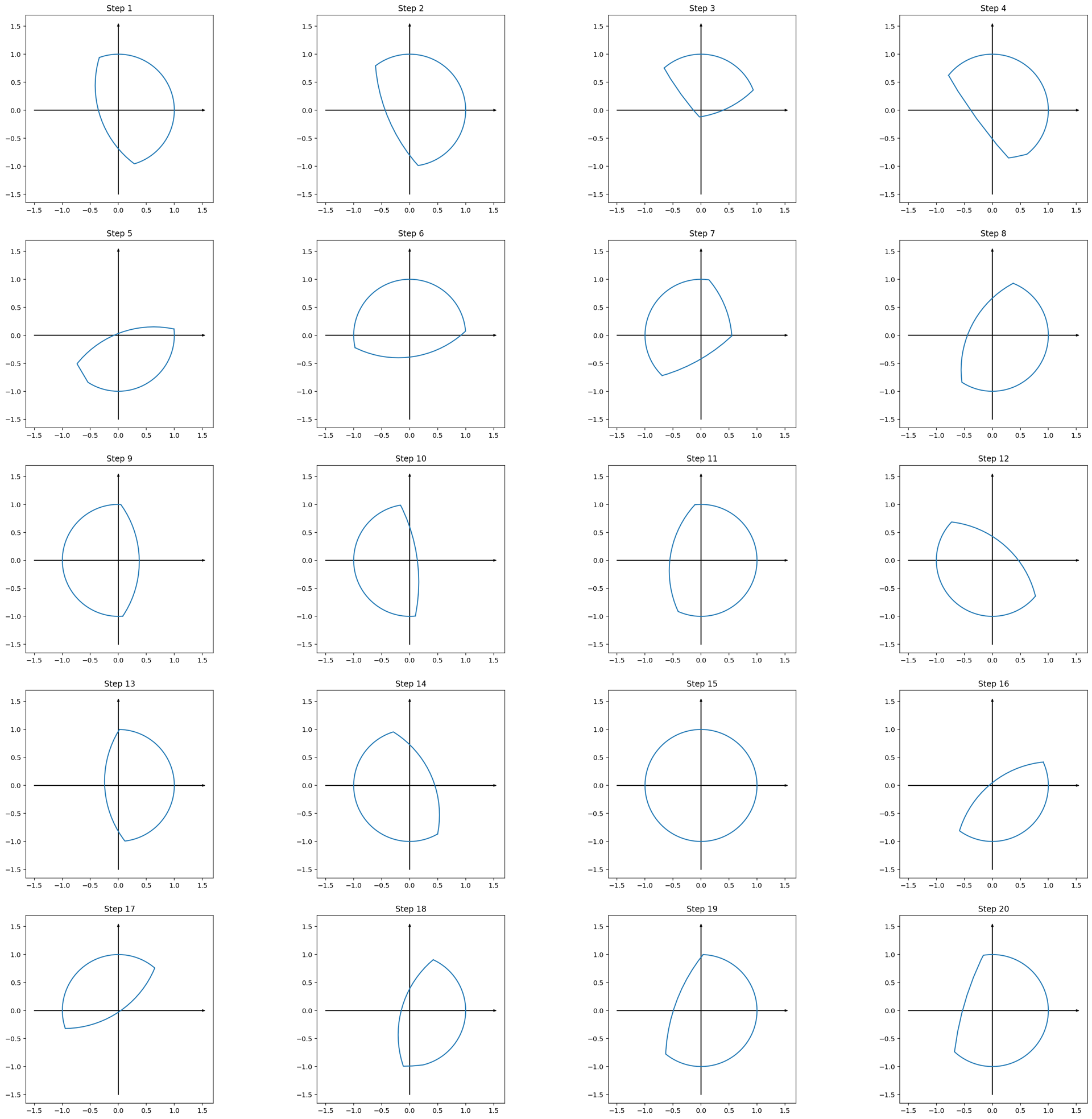
Figure 1. First twenty values of the chain $(X_{h})_{h\in\mathbb{N}_{0}}$ in $\mathbb{R}^{2}$ with the Euclidean norm and $\tau=4/7$. The chain starts at $B_{1}$ and returns to this state on Step 15. Each value of the chain is a finite intersection of translated and scaled unit balls.

The following observation is crucial for the proof that $(X_{h})$ is positive recurrent. It tells us that with probability one $X_{h}$ contains a ball of a small (but fixed) radius, for all sufficiently large $h\in\mathbb{N}_{0}$.

Proposition 3.3.

Let $K\in\mathcal{K}_{d}$ be an arbitrary compact convex body which contains a ball of radius $\varepsilon>0$. Put $r:=\min(\varepsilon,1)2^{-d-1}$. Then

(9) $$\mathbb{P}\{X_{h}\ominus B_{r}\neq\varnothing\text{ for all }h\in\mathbb{N}_{0}|X_{0}=K\}=1.$$

Proof.

Without loss of generality assume that $K$ contains the origin in its interior and $B_{\varepsilon}\subset K$. Moreover, starting with $X_{1}$, we can assume that $K\subset B_{1}$. For notational simplicity put $\mathcal{U}_{k}(X_{k})=:u_{k}$, $k\in\mathbb{N}_{0}$, so, let us repeat again,

$$X_{0}=K,\quad X_{h+1}=\tau^{-1}(X_{h}-u_{h})\cap B_{1},\quad h\in\mathbb{N}_{0}.$$

By induction,

(10) $$X_{h}=\left(\tau^{-h}K-\sum_{j=1}^{h}\tau^{-j}u_{h-j}\right)\bigcap\left(\bigcap_{k=0}^{h-1}\left(B_{\tau^{-k}}-\sum_{j=1}^{k}\tau^{-j}u_{h-j}\right)\right)=:\widehat{K}^{(h)}\cap\widehat{B}^{(h)},\quad h\in\mathbb{N}_{0}.$$

Note that if the upper index is strictly smaller than the lower one, then intersections are set to be equal to $\mathbb{R}^{d}$ and sums are set to vanish. We show that

(11) $$(\widehat{K}^{(h)}\cap\widehat{B}^{(h)})\ominus B_{r}\neq\varnothing,\quad h\geq d.$$

Fix any $h\geq d$. Upon multiplying by $\tau^{h}$, this is equivalent to

(12) $$\varnothing\neq\left(K\ominus B_{\tau^{h}r}-\sum_{j=0}^{h-1}\tau^{j}u_{j}\right)\bigcap\left(\bigcap_{k=0}^{h-1}\left(B_{\tau^{h-k}-\tau^{h}r}-\sum_{j=h-k}^{h-1}\tau^{j}u_{j}\right)\right)\\ =:\bigcap_{k=0}^{h}\Big{(}L^{(k)}-v_{h,k}\Big{)},$$

where $L^{(0)}:=K\ominus B_{\tau^{h}r}$ and $L^{(k)}:=B_{\tau^{k}-\tau^{h}r}$ for $k=1,\dots,h$, and

$$v_{h,k}:=\sum_{j=k}^{h-1}\tau^{j}u_{j},\quad k=0,\dots,h.$$

Since $u_{h}\in X_{h}\subset\tau^{-h}K-\sum_{j=1}^{h}\tau^{-j}u_{h-j}$ and $\tau^{h}u_{h}+v_{h,0}=v_{h+1,0}$, we have

(13) $$v_{h,0}\in K\subset B_{1},\quad h\in\mathbb{N}.$$

Furthermore,

$$\tau^{h}u_{h}\in(L^{(k)}-v_{h,k})\subset(B_{\tau^{k}}-v_{h,k}),$$

so that $\|v_{h,k}\|\leq\tau^{k}$ for all $k\leq h$. Furthermore,

(14) $$\|v_{h,k}-v_{h,l}\|=\|v_{l,k}\|\leq\tau^{k},\quad 1\leq k<l\leq h,\quad h\in\mathbb{N}.$$

In order to check (12), we employ Helly’s theorem, see [1, Theorem I.4.3], which tells us that the intersection of a finite family of convex sets in $\mathbb{R}^{d}$ is non-empty if an intersection of any $d+1$ sets in this family is non-empty. Fix $0\leq i_{0}<i_{1}<\cdots<i_{d}\leq h$, and put

$$\lambda_{j}:=\frac{2^{j}\tau^{-i_{j}}}{\sum_{j=0}^{d}2^{j}\tau^{-i_{j}}},\quad j=0,\ldots,d.$$

We aim to show that

$$-\sum_{k=0}^{d}\lambda_{k}v_{h,i_{k}}\in\bigcap_{j=0}^{d}\Big{(}L^{(i_{j})}-v_{h,i_{j}}\Big{)},\quad h\geq d+1.$$

If $i_{0}\geq 1$, it suffices to check that

(15) $$\left\|\sum_{k=0}^{d}\lambda_{k}v_{h,i_{k}}-v_{h,i_{j}}\right\|\leq\tau^{i_{j}}-r\tau^{h},\quad j=0,\ldots,d,\quad h\geq d+1.$$

By (14),

$$\|v_{h,i_{k}}-v_{h,i_{j}}\|\leq\tau^{\min(i_{k},i_{j})}.$$

Thus, for every fixed $j=0,\ldots,d$,

$$\left\|\sum_{k=0}^{d}\lambda_{k}v_{h,i_{k}}-v_{h,i_{j}}\right\| \leq\sum_{k=0}^{j-1}\lambda_{k}\|v_{h,i_{k}}-v_{h,i_{j}}\|+\sum_{k=j+1}^{d}\lambda_{k}\|v_{h,i_{k}}-v_{h,i_{j}}\|$$

$$\leq\frac{1}{\sum_{k=0}^{d}2^{k}\tau^{-i_{k}}}\left(\sum_{k=0}^{j-1}2^{k}\tau^{-i_{k}}\tau^{i_{k}}+\tau^{i_{j}}\sum_{k=j+1}^{d}2^{k}\tau^{-i_{k}}\right)$$

$$=\frac{1}{\sum_{k=0}^{d}2^{k}\tau^{-i_{k}}}\left(2^{j}-1+\tau^{i_{j}}\sum_{k=j+1}^{d}2^{k}\tau^{-i_{k}}\right),$$

where the last sum in parentheses is zero if $j=d$. This estimate demonstrates that (15) is a consequence of

(16) $$2^{j}+r\tau^{h}\sum_{k=0}^{d}2^{k}\tau^{-i_{k}}\leq 1+\tau^{i_{j}}\sum_{k=0}^{j}2^{k}\tau^{-i_{k}},\quad j=0,\ldots,d,\quad h\geq d.$$

It remains to note that we have chosen $r\leq 2^{-d-1}$, so that

$$2^{j}+r\tau^{h}\sum_{k=0}^{d}2^{k}\tau^{-i_{k}}\leq 2^{j}+r\sum_{k=0}^{d}2^{k}\leq 2^{j}+1\leq 1+\tau^{i_{j}}\sum_{k=0}^{j}2^{k}\tau^{-i_{k}},$$

which implies (16).

Now assume that $i_{0}=0$. Then (15) holds for $j=1,\dots,d$ and we need to consider

(17) $$-\sum_{k=0}^{d}\lambda_{k}v_{h,i_{k}}+v_{h,0}=\sum_{k=1}^{d}\lambda_{k}(v_{h,0}-v_{h,i_{k}})=\sum_{k=1}^{d}\lambda_{k}v_{i_{k},0}.$$

Since $v_{i_{k},0}\in K$ for all $k\geq 1$ by (13), the sum on the right-hand side belongs to $(1-\lambda_{0})K$. Thus, the left-hand side of (17) belongs to $L^{(0)}=K\ominus B_{\tau^{h}r}$ if

$$(1-\lambda_{0})K+B_{\tau^{h}r}\subset K,$$

equivalently,

(18) $$B_{r}\subset\lambda_{0}\tau^{-h}K.$$

Since

$$\lambda_{0}\tau^{-h}K=\frac{\tau^{-h}}{\sum_{j=0}^{d}2^{j}\tau^{-{i_{j}}}}K=\frac{1}{\sum_{j=0}^{d}2^{j}\tau^{h-{i_{j}}}}K\supset 2^{-(d+1)}K,$$

(18) holds for $r=\varepsilon 2^{-d-1}$ if $K$ contains $B_{\varepsilon}$.

If $h<d$, we add fictitious balls $B_{1}$ to the intersection (10), note that $v_{h,k}=0$ for $k\geq h+1$, and repeat the arguments. ∎

Proposition 3.3 is essential to prove the following result, which shows that $(X_{h})_{h\in\mathbb{N}_{0}}$ is a recurrent Harris chain.

Proposition 3.4.

Assume that $X_{0}=K$ for some $K\in\mathcal{K}_{d}$. Let

$$\kappa^{(0)}_{B_{1}}:=\min\{h\in\mathbb{N}_{0}:X_{h}=B_{1}\},\quad\kappa^{(i)}_{B_{1}}:=\min\{h>\kappa^{(i-1)}_{B_{1}}:X_{h}=B_{1}\},\quad i\in\mathbb{N}.$$

Then $\mathbb{P}\{\kappa^{(0)}_{B_{1}}<\infty\}=1$ and $(\kappa^{(i)}_{B_{1}}-\kappa^{(i-1)}_{B_{1}})_{i\in\mathbb{N}}$ are independent identically distributed with

$$\mathbb{E}\left(\kappa^{(i)}_{B_{1}}-\kappa^{(i-1)}_{B_{1}}\right)<\infty,\quad i\in\mathbb{N}.$$

Proof.

Let

$$r_{h}:=\sup\{t\geq 0:X_{h}\ominus B_{t}\neq\varnothing\},\quad h\in\mathbb{N}_{0},$$

be the radius of the largest ball inscribed in $X_{h}$. By Proposition 3.3, $r_{h}\in[r,1]$ for all $h\in\mathbb{N}_{0}$. Fix $\delta\in(\tau,1)$ and define the events

$$A_{h}(\delta):=\{\mathcal{U}_{h}(X_{h})\in X_{h}\ominus B_{\delta r_{h}}\}=\{B_{\delta r_{h}}\subset X_{h}-\mathcal{U}_{h}(X_{h})\},\quad h\in\mathbb{N}_{0}.$$

Note that, for $t\in(0,1]$,

$$\{r_{h+m+1}\geq t\} =\{X_{h+m+1}\ominus B_{t}\neq\varnothing\}$$

$$\supset\{(\tau^{-1}(X_{h+m}-\mathcal{U}_{h+m}(X_{h+m}))\cap B_{1})\ominus B_{t}\neq\varnothing\}\cap A_{h+m}(\delta)$$

$$\supset\{(\tau^{-1}B_{\delta r_{h+m}}\cap B_{1})\ominus B_{t}\neq\varnothing\}\cap A_{h+m}(\delta)$$

$$=\{\tau^{-1}\delta r_{h+m}\geq t\}\cap A_{h+m}(\delta).$$

Iterating this inclusion we arrive at

(19) $$\{r_{h+m+1}\geq t\}\supset\{r_{h}\geq t(\tau/\delta)^{m+1}\}\cap\bigcap_{k=0}^{m}A_{h+k}(\delta),\quad h,m\in\mathbb{N}_{0}.$$

Define $m_{0}:=\inf\{k\in\mathbb{N}_{0}:(\tau/\delta)^{k+1}\leq r\}$ and plug $t=1$ into (19). Since $r_{h}\geq r$, this yields

(20) $$\{X_{h+m_{0}+1}=B_{1}\}=\{r_{h+m_{0}+1}=1\}\supset\bigcap_{k=0}^{m_{0}}A_{h+k}(\delta),\quad h\in\mathbb{N}_{0}.$$

Suppose that

(21) $$\mathbb{P}\left\{\bigcap_{k=0}^{m_{0}}A_{h+k}(\delta)\Big{|}X_{h}\in\cdot\right\}\geq p^{\ast},\quad h\in\mathbb{N}_{0},$$

for a positive constant $p^{\ast}$. Inclusion (20) demonstrates that from any state $X_{h}$ with probability at least $p^{\ast}$ the chain $(X_{h})$ visits the state $B_{1}$ after exactly $m_{0}+1$ steps. Dividing the entire trajectory of $(X_{h})$ into consecutive blocks of size $m_{0}+1$, we see that the distribution of $\kappa_{B_{1}}$ (conditional, given $X_{0}=B_{1}$) is stochastically dominated by the product of the constant $(m_{0}+1)$ and a geometrically distributed random variable with success probability $p^{\ast}$.

It remains to confirm (21). We have

(22) $$\mathbb{P}\left\{\bigcap_{k=0}^{m_{0}}A_{h+k}(\delta)\Big{|}X_{h}\in\cdot\right\}=\prod_{k=0}^{m_{0}}\mathbb{P}\left\{A_{h+k}(\delta)\big{|}\cap_{j=0}^{k-1}A_{h+j}(\delta),X_{h}\in\cdot\right\}.$$

Let $\sigma_{h}$ be the $\sigma$-algebra generated by $\{\mathcal{U}_{0},\mathcal{U}_{1},\ldots,\mathcal{U}_{h-1}\}$, $h\in\mathbb{N}$. By the construction, $X_{h}$ is $\sigma_{h}$-measurable and $A_{h}(\delta)$ belongs to $\sigma_{h+1}$. Therefore, $\cap_{j=0}^{k-1}A_{h+j}(\delta)\cap\{X_{h}\in\cdot\}$ is $\sigma_{h+k}$-measurable.

Let $A$ be an arbitrary event from $\sigma_{h+k}$. By the definition of $r_{h+k}$, there exists a $\sigma_{h+k}$-measurable point $c_{h+k}$ such that $B_{(1-\delta)r_{h+k}}(c_{h+k})\subset X_{h+k}\ominus B_{\delta r_{h+k}}$. Since $\mathcal{U}_{h+k}$ is independent of $\sigma_{h+k}$ and $(X_{h+k},r_{h+k},c_{h+k})$ is $\sigma_{h+k}$-measurable,

$$\mathbb{P}\big{\{}A_{h+k}(\delta)\,|\,A\big{\}} =\mathbb{P}\big{\{}A_{h+k}(\delta)\,|\,A\big{\}}=\mathbb{P}\big{\{}\mathcal{U}_{h+k}(X_{h+k})\in X_{h+k}\ominus B_{\delta r_{h+k}}\,|\,A\big{\}}$$

$$\geq\mathbb{P}\big{\{}\mathcal{U}_{h+k}(X_{h+k})\in B_{(1-\delta)r_{h+k}}(c_{h+k})\,|\,A\big{\}}$$

$$=\frac{1}{\mathbb{P}\{A\}}\mathbb{E}\left(\mathbb{E}\left(\frac{\lambda\big{(}B_{(1-\delta)r_{h+k}}(c_{h+k})\big{)}}{\lambda(X_{h+k})}\mathbbm{1}_{A}\Big{|}\sigma_{h+k}\right)\right)$$

$$\geq\frac{1}{\mathbb{P}\{A\}}\mathbb{E}\left(\mathbb{E}\left(\frac{\lambda\big{(}B_{(1-\delta)r}\big{)}}{\lambda(B_{1})}\mathbbm{1}_{A}\Big{|}\sigma_{h+k}\right)\right)$$

$$=\frac{\lambda(B_{(1-\delta)r})}{\lambda(B_{1})}=\big{(}(1-\delta)r\big{)}^{d}>0.$$

This bound implies (21) in view of (22). ∎

Proof of Theorem 2.2.

The result follows from Theorem 6.8.8 in [5] in conjunction with Proposition 3.4. Note that the chain $(X_{h})_{h\in\mathbb{N}_{0}}$ is aperiodic by (8). The limit distribution is given (implicitly) by

$$\mathbb{P}\{J_{\infty}\in\cdot\}=\frac{1}{\mathbb{E}\big{(}\kappa^{(1)}_{B_{1}}-\kappa^{(0)}_{B_{1}}\big{)}}\mathbb{E}\left(\sum_{h\geq 0}\mathbbm{1}_{\{X_{h}\in\cdot,\kappa^{(0)}_{B_{1}}\leq h<\kappa^{(1)}_{B_{1}}\}}\right).$$

The fact that $J_{\infty}$ is a finite intersection of balls with radii $\{1,\tau^{-1},\tau^{-2},\ldots\}$ with probability one follows from (10) and $\mathbb{P}\big{\{}\kappa^{(1)}_{B_{1}}-\kappa^{(0)}_{B_{1}}<\infty\big{\}}=1$. ∎

4. The length of the leftmost path

Recall that the left boundary of a vp tree $\mathbb{VP}(x_{1},x_{2},\ldots)$ is the unique path which starts at the root and on each step follows the left subtree. Also recall the notation $(x_{l_{h}},r_{x_{l_{h}}})$ for the vertex of depth $h\in\{0,1,2,\ldots\}$ and its threshold in this path and $(I_{h})_{h\in\mathbb{N}_{0}}$ for the sequence defined in (4).

We are interested in the number $L_{n}$ of edges in the leftmost path of $\mathbb{VP}(U_{1},U_{2},\ldots,U_{n})$ with exponential threshold function (1). Let $l_{1}-l_{0}$ be the number of trials (insertions of new vertices) until a left child is attached to the root. Obviously, given $I_{1}$, $l_{1}-l_{0}$ has a geometric law on $\mathbb{N}$ with success probability $\lambda(I_{1})/\lambda(K)$. Similarly, given $(I_{h})_{h=0,\ldots,k}$, $l_{k}-l_{k-1}$ has a geometric law on $\mathbb{N}$ with success probability $\lambda(I_{k})/\lambda(K)$, and $l_{1}-l_{0},l_{2}-l_{1},\ldots,l_{k}-l_{k-1}$ are conditionally independent. According to Proposition 2.1 and the discussion afterwards, the distribution of the sequence $(l_{k}-l_{k-1})_{k\in\mathbb{N}}$ is the same as that of the sequence $(G_{k})_{k\in\mathbb{N}}$ comprised of conditionally independent, given $(\widetilde{J}_{h})_{h\in\mathbb{N}_{0}}$, random variables such that

$$\mathbb{P}\{G_{k}=j\,|\,\widetilde{J}_{0},\ldots,\widetilde{J}_{k}\}=\frac{\lambda(\widetilde{J}_{k})}{\lambda(K)}\left(1-\frac{\lambda(\widetilde{J}_{k})}{\lambda(K)}\right)^{j-1},\quad j\in\mathbb{N},\quad k\in\mathbb{N}.$$

Put $S_{0}:=0$ and $S_{k}:=G_{1}+G_{2}+\cdots+G_{k}$, $k\in\mathbb{N}$. Notice that the sequence $(1+S_{k})_{k\in\mathbb{N}_{0}}$ is distributed as the sequence of time epochs when new vertices are attached to the leftmost path. Thus, see also Eq. (24) in [4],

(23) $$L_{n}\overset{d}{=}\max\{k\in\mathbb{N}_{0}:1+S_{k}\leq n\},\quad n\in\mathbb{N}.$$

To derive a limit theorem for $L_{n}$ we start with a couple of lemmas.

Lemma 4.1.

For every fixed $l\in\mathbb{N}_{0}$, we have

$$\tau^{-n}\left(\widetilde{J}_{n},\widetilde{J}_{n-1},\ldots,\widetilde{J}_{n-l}\right)~{}\stackrel{{\scriptstyle d}}{{\longrightarrow}}~{}(J_{\infty}^{(0)},J_{\infty}^{(1)},\ldots,J_{\infty}^{(l)})\quad\text{as}\;n\to\infty.$$

The limit sequence $(J_{\infty}^{(h)})_{h\in\mathbb{N}_{0}}$ is defined as follows: $(\tau^{h}J_{\infty}^{(h)})_{h\in\mathbb{N}_{0}}$ is a stationary sequence of consecutive values of a Markov chain (7) which starts at the stationary distribution $J_{\infty}$ defined in Theorem 2.2.

Proof.

Follows immediately from Theorem 2.2. ∎

It is known that the volume mapping $\lambda:\mathcal{K}_{d}\mapsto[0,\infty)$ is continuous with respect to the Hausdorff metric, see Theorem 1.8.20 in [12]. Therefore, for every fixed $l\in\mathbb{N}_{0}$,

(24) $$\tau^{-dn}\left(\frac{\lambda(\widetilde{J}_{n})}{\lambda(K)},\frac{\lambda(\widetilde{J}_{n-1})}{\lambda(K)},\ldots,\frac{\lambda(\widetilde{J}_{n-l})}{\lambda(K)}\right)~{}\stackrel{{\scriptstyle d}}{{\longrightarrow}}~{}\left(\frac{\lambda(J_{\infty}^{(0)})}{\lambda(K)},\frac{\lambda(J_{\infty}^{(1)})}{\lambda(K)},\ldots,\frac{\lambda(J_{\infty}^{(l)})}{\lambda(K)}\right)\quad\text{as}\;n\to\infty.$$

Given, $(J_{\infty}^{(h)})_{h\in\mathbb{N}_{0}}$, let $(\mathcal{E}_{l})_{l\in\mathbb{N}_{0}}$ be a sequence of conditionally independent random variables with the exponential distributions

$$\mathbb{P}\{\mathcal{E}_{l}\geq t\,|\,(J_{\infty}^{(h)})_{h\geq 0}\}=\exp\left(-t\frac{\lambda(J_{\infty}^{(l)})}{\lambda(K)}\right),\quad t\geq 0,\quad l\in\mathbb{N}_{0}.$$

Lemma 4.2.

The random series $S_{\infty}:=\sum_{l=0}^{\infty}\mathcal{E}_{l}$ converges a.s. and in mean.

Proof.

The claims follow from

$$\sum_{l=0}^{\infty}\mathbb{E}(\mathcal{E}_{l})=\sum_{l=0}^{\infty}\mathbb{E}(\mathbb{E}(\mathcal{E}_{l}|(J_{\infty}^{(h)})_{h\geq 0}))=\lambda(K)\sum_{l=0}^{\infty}\mathbb{E}\left(\frac{1}{\lambda(J_{\infty}^{(l)})}\right)\\ =\lambda(K)\sum_{l=0}^{\infty}\tau^{ld}\mathbb{E}\left(\frac{1}{\lambda(\tau^{l}J_{\infty}^{(l)})}\right)=\lambda(K)\mathbb{E}\left(\frac{1}{\lambda(J_{\infty})}\right)\frac{1}{1-\tau^{d}}<\infty,$$

where we have used stationarity of $(\tau^{h}J_{\infty}^{(h)})_{h\in\mathbb{N}_{0}}$. The fact that $\mathbb{E}\left(\frac{1}{\lambda(J_{\infty})}\right)<\infty$ is a consequence of Proposition 3.3 which implies that $\lambda(J_{\infty})$ is bounded away from zero. ∎

Lemma 4.3.

As $n\to\infty$, it holds

(25) $$\tau^{dn}S_{n}~{}\stackrel{{\scriptstyle d}}{{\longrightarrow}}~{}\sum_{l=0}^{\infty}\mathcal{E}_{l}=S_{\infty}.$$

Proof.

According to Proposition 3.3, there exist $0<c_{1}<c_{2}<\infty$ such that

(26) $$\mathbb{P}\left\{c_{1}\tau^{dh}\leq\frac{\lambda(\widetilde{J}_{h})}{\lambda(K)}\leq c_{2}\tau^{dh},h\in\mathbb{N}_{0}\right\}=1.$$

Put $Z_{n}(t):=\mathbb{E}\left(e^{it\tau^{dn}S_{n}}\,|\,\widetilde{J}_{0},\ldots,\widetilde{J}_{n}\right)$. It suffices to show that, for every fixed $t\in\mathbb{R}$,

(27) $$Z_{n}(t)~{}\stackrel{{\scriptstyle d}}{{\longrightarrow}}~{}\prod_{h=0}^{\infty}\frac{1}{1-\lambda(K)it/\lambda(J_{\infty}^{(h)})}\quad\text{as}\;n\to\infty.$$

The convergence (27) yields (25) by the Lebesgue dominated convergence theorem.

Let $\log$ denote the principal branch of the complex logarithm. For fixed $t\in\mathbb{R}$ and using (26), we obtain

$$-\log Z_{n}(t) =\sum_{h=1}^{n}\log\left(1-\frac{\lambda(K)}{\lambda(\widetilde{J}_{h})}(1-e^{-it\tau^{nd}})\right)$$

$$=\sum_{h=1}^{n}\log\left(1-\frac{\lambda(K)}{\lambda(\widetilde{J}_{h})}(it\tau^{nd}+O(\tau^{2nd}))\right)=\sum_{h=1}^{n}\log\left(1-\frac{\lambda(K)}{\lambda(\widetilde{J}_{h})}it\tau^{nd}\right)+o(1),$$

where $o(1)$ is a non-random sequence which converges to zero as $n\to\infty$. Further,

$$\sum_{h=1}^{n}\log\left(1-\frac{\lambda(K)}{\lambda(\widetilde{J}_{h})}it\tau^{nd}\right) =\sum_{h=0}^{n-1}\log\left(1-\frac{\lambda(K)}{\tau^{-nd}\lambda(\widetilde{J}_{n-h})}it\right)$$

$$=\left(\sum_{h=0}^{M}+\sum_{h=M+1}^{n-1}\right)\log\left(1-\frac{\lambda(K)}{\tau^{-nd}\lambda(\widetilde{J}_{n-h})}it\right)=:A_{n,M}(t)+B_{n,M}(t).$$

By Lemma 4.1 we have

$$A_{n,M}(t)~{}\stackrel{{\scriptstyle d}}{{\longrightarrow}}~{}\sum_{h=0}^{M}\log\left(1-\lambda(K)it/\lambda(J_{\infty}^{(h)})\right),\quad n\to\infty,$$

for every fixed $M\in\mathbb{N}$. As $M\to\infty$, $e^{-A_{n,M}(t)}$ converges to the right-hand side of (27). According to Theorem 3.2 in [3] it remains to check that, for every fixed $\varepsilon>0$,

(28) $$\lim_{M\to\infty}\limsup_{n\to\infty}\mathbb{P}\big{\{}|B_{n,M}(t)|\geq\varepsilon\,|\,\widetilde{J}_{0},\ldots,\widetilde{J}_{n}\}=0\quad\text{a.s.}$$

Using (26) we infer, for some $C>0$,

$$|B_{n,M}(t)|\leq\sum_{h=M+1}^{n-1}\left|\log\left(1-\frac{\lambda(K)}{\tau^{-nd}\lambda(\widetilde{J}_{n-h})}it\right)\right| \leq C|t|\sum_{h=M+1}^{n-1}\frac{\lambda(K)}{\tau^{-nd}\lambda(\widetilde{J}_{n-h})}$$

$$\overset{\eqref{eq:two_sided_bound_volumes}}{\leq}Cc_{1}^{-1}|t|\sum_{h=M+1}^{n-1}\tau^{hd}.$$

This clearly implies (28) and the proof is complete. ∎

Combining the above lemmas and the duality relation (23) we arrive at the following result.

Theorem 4.4.

Under the same assumptions as in Theorem 2.2, for every fixed $x>0$, it holds

$$\lim_{n\to\infty}\mathbb{P}\big{\{}L_{\lfloor x\tau^{-nd}\rfloor}\leq n+s\big{\}}=\mathbb{P}\big{\{}S_{\infty}\geq x\tau^{sd}\big{\}}=\mathbb{P}\left\{\frac{\log S_{\infty}-\log x}{d\log\tau}\leq s\right\},\quad s\in\mathbb{Z},$$

where $S_{\infty}$ is defined in Lemma 4.2.

Proof.

Fix $s\in\mathbb{Z}$, $x>0$ and write

$$\mathbb{P}\big{\{}L_{\lfloor x\tau^{-nd}\rfloor}>n+s\big{\}}=\mathbb{P}\big{\{}1+S_{n+s}\leq\lfloor x\tau^{-nd}\rfloor\big{\}}=\mathbb{P}\big{\{}\tau^{(n+s)d}+\tau^{(n+s)d}S_{n+s}\leq\lfloor x\tau^{-nd}\rfloor\tau^{(n+s)d}\big{\}}.$$

It is easy to check that the distribution of $S_{\infty}$ is continuous. Thus, letting $n\to\infty$ yields that the right-hand side converges to $\mathbb{P}\{S_{\infty}\leq x\tau^{sd}\}=\mathbb{P}\{S_{\infty}<x\tau^{sd}\}$ by Lemma 4.3. ∎

Corollary 4.5.

The following weak laws of large numbers hold

$$\frac{\log S_{n}}{n}~{}\overset{\mathbb{P}}{\longrightarrow}~{}d\log(1/\tau)\quad\text{as}\;n\to\infty,$$

and

(29) $$\frac{L_{n}}{\log n}~{}\overset{\mathbb{P}}{\longrightarrow}~{}\frac{1}{d\log(1/\tau)}\quad\text{as}\;n\to\infty.$$

Remark 4.6.

Let $H_{n}$ be the height of $\mathbb{VP}(U_{1},U_{2},\ldots,U_{n})$ which is the length of the longest path from the root to a leaf. Since $L_{n}\leq H_{n}$, Theorem 4.4 implies

$$\lim_{n\to\infty}\mathbb{P}\left\{H_{n}\geq\left(\frac{1}{d\log(1/\tau)}-\varepsilon\right)\log n\right\}=1,$$

for every fixed $\varepsilon>0$. We conjecture that

(30) $$\frac{H_{n}}{\log n}~{}\overset{\mathbb{P}}{\longrightarrow}~{}H_{\infty},\quad n\to\infty,$$

for some finite deterministic constant $H_{\infty}\geq\frac{1}{d\log(1/\tau)}$.

References

[1]Barvinok A. (2002). A Course in Convexity,
Amer. Math. Soc., Providence, RI.
[2]Bentley, J. (1975). Multidimensional binary search trees used for associative searching. Commun. ACM18(9), pp. 509-517.
[3]Billingsley, P. (2013). Convergence of probability measures. John Wiley & Sons.
[4]Bohun, V. (2021). Probabilistic analysis of vantage point trees. Modern Stochastics: Theory and Applications, 8(4), pp. 413-434.
[5]Durrett, R. (2010). Probability: Theory and
Examples, edition, Cambridge University Press, Cambridge.
[6]Fu, A. W. C., Chan, P. M. S., Cheung, Y. L. and Moon, Y. S. (2000). Dynamic vp-tree indexing for -nearest neighbor search given pair-wise distances. The VLDB Journal, 9, pp. 154-173.
[7]Kevei, P. and Vígh, V. (2016). On the diminishing process of Bálint Tóth. Transactions of the American Mathematical Society, 368(12), pp. 8823-8848.
[8]Molchanov, I. (2015). Continued fractions built from convex sets and convex functions. Communications in Contemporary Mathematics17(05), 1550003.
[10]Nielsen, F., Piro, P. and Barlaud, M. (2009). Bregman vantage point trees for efficient nearest neighbor queries. In 2009 IEEE International Conference on Multimedia and Expo. pp. 878–881.