Closed-Loop Finite-Time Analysis of
Suboptimal Online Control

Abstract

Suboptimal methods in optimal control arise due to a limited computational budget, unknown system dynamics, or a short prediction window among other reasons. Although these methods are ubiquitous, their transient performance remains relatively unstudied. We consider the control of discrete-time, nonlinear time-varying dynamical systems and establish sufficient conditions to analyze the finite-time closed-loop performance of such methods in terms of the additional cost incurred due to suboptimality. Finite-time guarantees allow the control design to distribute a limited computational budget over a time horizon and estimate the on-the-go loss in performance due to suboptimality. We study exponential incremental input-to-state stabilizing policies, and show that for nonlinear systems, under some mild conditions, this property is directly implied by exponential stability without further assumptions on global smoothness. The analysis is showcased on a suboptimal model predictive control use case.

Nonlinear Systems, Optimization Algorithms, Predictive Control

1 Introduction

Optimal control aims to compute an input signal to drive a dynamical system to a given target state, while optimizing a performance cost subject to constraints. In the absence of uncertainty, the problem has been studied using calculus of variations [1] and dynamic programming [2]. However, in many practical applications with limited computational power, it becomes difficult or infeasible to solve due to the curse of dimensionality [2]. This is further exacerbated if there are unknown system and/or cost parameters. As a result, control designers rely on approximate or suboptimal methods [3] to solve the problem. If there are adequate computational resources and an accurate simulator of the true system, the problem can be solved up to an arbitrary accuracy using approximate dynamic programming [4] or reinforcement learning [5] techniques. When this is not the case, e.g. the system has unpredictable dynamics or the cost to be optimized for is changing adversarially, offline methods alone are not sufficient. In such cases, the input or the policy are updated online or adaptively as more data becomes available. Examples of such suboptimal online methods include adaptive controllers [6, 7], receding horizon controllers [8, 9], online control methods [10, 11] or online feedback optimization methods [12, 13].

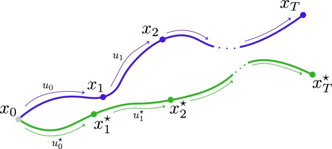
Figure 1: Two separate trajectories generated by applying respectively suboptimal and optimal input signals.

Suboptimal online algorithms become a necessity driven by practical requirements. This motivates research on the performance of such methods, especially in the finite-time or transient domain. Given their implementation in real-time implementation, suboptimal algorithms need to stay computationally efficient while stabilizing the system. Additionally, their performance is measured in terms of the accumulated cost that needs to be kept to a minimum. To quantify this, we fix a benchmark policy that we deem to be close to the desired optimal one, visualized in Figure 1, and study the suboptimality gap of the given algorithm in terms of the additional incurred cost due to suboptimality. Such an analysis provides a relative measure on the performance of the given algorithm, since, in general, the benchmark policy attains a non-zero cost. In this context, we pose the following questions.

1. How does the transient cost performance of an online algorithm scale with a measure of its suboptimality?

2. How should the benchmark policy be chosen to achieve computable and meaningful finite-time bounds?

We consider nonlinear time-varying systems and choose a benchmark policy that renders the closed-loop system exponentially incrementally input-to-state stable (E-$\delta$-ISS). Incremental input-to-state stability has been introduced in [14], in the continuous-time setting and later analyzed in discrete-time in [15]. As opposed to input-to-state stability, E-$\delta$-ISS provides a condition on the deviation of two separate trajectories of the same system. A sufficient condition for E-$\delta$-ISS to hold is that of contraction [16, 17, 18]. When the dynamics are smooth, contraction can be verified by checking uniform negative definiteness conditions [17, 16]. However, smoothness often does not hold for the closed-loop dynamics; this is the case, for example, for linear time-invariant systems in closed-loop with a constrained Model Predictive Controller (MPC) [19]. Here we consider general nonlinear systems that are smooth only in an arbitrarily small region around the origin. Contraction can also be asserted, at least in the continuous-time case, by ensuring the closed-loop system is one-sided Lipschitz continuous [20, 18]. We do not explore this condition for our use cases and instead start with the assumption that the closed-loop dynamics under the benchmark policy are exponentially stable, which is often easier to verify.

There are several notable examples of settings where such finite-time suboptimality analysis of an online algorithm can be applied. These include suboptimal MPC, e.g. [8, 21, 22], when the suboptimality is due to finite computational resources, adaptive controllers with transient performance guarantees, e.g. [6, 11], with suboptimality due to unknown system parameters, or online feedback optimization [12, 13] and online control [10, 11], with suboptimality due to unknown future costs. In this work, we study the suboptimal linear quadratic MPC (LQMPC) setting in detail and show how a nonlinear incremental stability analysis can be used to provide a tighter bound on the suboptimality gap as compared to the one derived in [23].

Our contributions are summarized below:

1. We derive sufficient conditions under which exponential stability (ES)of a non-smooth nonlinear time-varying system implies E-$\delta$-ISS, making the condition on the benchmark policy easier to verify,

2. We show that if the closed-loop dynamics in closed-loop with the benchmark policy are E-$\delta$-ISS, then the suboptimality gap scales with the pathlength of closed-loop suboptimal trajectory,

3. We study suboptimal LQMPC as an example satisfying these assumptions.

Our bounds are asymptotically tight, in the sense that they scale with the level of suboptimality of the given algorithm, converging to zero when the algorithm matches with the benchmark. The bounds also scale with the pathlength of the suboptimal trajectory, allowing an on-the-go calculation of the suboptimality gap that is independent of the optimal states. Moreover, our result is independent of the asymptotic properties of the suboptimal algorithm, providing finite-time performance bounds even when the closed-loop is not exponentially stable.

The article is structured as follows. In Section 2 we provide the preliminaries and the problem setup. In Section 3, we conduct the suboptimality gap analysis. Sufficient conditions for E-$\delta$-ISS are derived in Section 4, and in Section 5, the suboptimal MPC use case with a numerical example is studied.

Notation: The sets of positive real numbers, positive integers and non-negative integers are denoted by $\mathbb{R}_{+}$, $\mathbb{N}_{+}$ and $\mathbb{N}$, respectively. For a given vector $x$, its Euclidean norm is denoted by $\|x\|$, and the two-norm weighted by a $Q\succ 0$ by $\|x\|_{Q}=\sqrt{x^{\top}Qx}$. For a square matrix $W$, the spectral radius and the spectral norm are denoted by $\rho(W)$, and $\|W\|$, respectively. Given $M\succ 0$, $\lambda_{M}^{-}(W)$ and $\lambda_{M}^{+}(W)$ denote the minimum and maximum eigenvalues of ${M}^{-\frac{1}{2}}W{M}^{-\frac{1}{2}}$; for any vector $x$, they satisfy $\lambda_{M}^{-}(W)\|x\|_{M}^{2}\leq\|x\|_{W}^{2}\leq\lambda_{M}^{+}(W)\|x\|_{M}^{2}$. The Euclidean point-to-set distance of a vector $x$ from a nonempty, closed, convex set $\mathcal{A}$ is denoted by $|x|_{\mathcal{A}}:=\min_{y\in\mathcal{A}}\|x-y\|$, and the projection onto it by $\Pi_{\mathcal{A}}[x]=\operatorname*{arg\,min}_{y\in\mathcal{A}}\|x-y\|$.

2 Preliminaries and Problem Setup

We consider the optimal control problem of discrete-time, nonlinear time-varying systems of the form

$$x_{k+1}=f_{0}(k,x_{k})+g(k,x_{k},u_{k}),\quad k\in\mathbb{N},$$ (1)

where $x_{k}\in\mathbb{R}^{n}$ and $u_{k}\in\mathbb{R}^{m}$ denote the state and control input at time $k$, respectively, $f_{0}:\mathbb{N}\times\mathbb{R}^{n}\rightarrow\mathbb{R}^{n}$ denotes the unforced nominal dynamics and $g:\mathbb{N}\times\mathbb{R}^{n}\times\mathbb{R}^{m}\rightarrow\mathbb{R}^{n}$ the controllable dynamics. Given an initial state $x_{0}\in\mathbb{R}^{n}$, the optimal control objective is to find the sequence of control inputs $\boldsymbol{u}=[u_{0}^{\top}\ldots u_{T-1}^{\top}]^{\top}$ that minimizes the finite-time cost

$$J_{T}(x_{0},\boldsymbol{u})=\sum_{k=0}^{T}c_{k}(x_{k},u_{k}),$$ (2)

where $c_{k}:\mathbb{R}^{n}\times\mathbb{R}^{m}\longrightarrow\mathbb{R}$ is the stage cost at time $k$. In addition, the control input has to satisfy $u_{k}\in\mathcal{U}$ for all $k$, for some bounded $\mathcal{U}\subset\mathbb{R}^{m}$.

Admissable policy $\pi(k,x):\mathbb{N}\times\mathbb{R}^{n}\rightarrow\mathcal{U}$ maps the current state and time $k$ to a control input, generating the control signal $\boldsymbol{u}^{\pi}=[u_{0}^{\pi\top}\ldots u_{T-1}^{\pi\top}]^{\top}$ and the associated trajectory $\boldsymbol{x}^{\pi}=[x_{0}^{\pi\top}\ldots x_{T}^{\pi\top}]^{\top}$ for a horizon of length $T$. With a slight abuse of notation, its associated cost is denoted by $J_{T}(x_{0},\pi)$. We consider time-varying systems for generality, and for the introduction of several novel results. Our analysis extends to time-invariant systems directly, as we showcase in Section 5.

We are interested in the relation of a policy $\mu$, corresponding to a given suboptimal algorithm, with respect to another benchmark policy $\mu^{*}$ that is equipped with desirable characteristics, such as optimality. The latter is often obtained as the solution of some optimization problem. The two policies are defined as follows.

Benchmark dynamics: Consider a benchmark policy $\mu^{\star}:\mathbb{N}\times\mathbb{R}^{n}\rightarrow\mathcal{U}$. In particular, given a $x_{0}^{\star}\in\mathbb{R}^{n}$, the benchmark dynamics are given by

$$x^{\star}_{k+1}=f_{0}(k,x_{k}^{\star})+g(k,x_{k}^{\star},\mu_{k}^{\star}(x_{k}^{\star})):=f(k,x^{\star}_{k}),$$ (3)

for all $k\in\mathbb{N}$. We assume that the closed-loop dynamics (3) define a forward invariant set $\mathcal{D}^{\star}\subseteq\mathbb{R}^{n}$, and restrict attention to $x_{0}^{\star}\in\mathcal{D}^{\star}$; hence $x_{k}^{\star}\in\mathcal{D}^{\star}$ for all $k\in\mathbb{N}$.

Suboptimal dynamics: The suboptimal state evolution for a given policy $\mu:\mathbb{N}\times\mathbb{R}^{n}\rightarrow\mathcal{U}$ can be represented in the following form for any $x_{0}\in\mathbb{R}^{n}$

$$\begin{split}x_{k+1}=f(k,x_{k})+\underbrace{g(k,x_{k},\mu_{k}(x_{k}))-g(k,x_{k},\mu_{k}^{\star}(x_{k}))}_{w_{k}(x_{k})},\end{split}$$ (4)

for all $k\in\mathbb{N}$. The mapping $w:\mathbb{N}\times\mathbb{R}^{n}\rightarrow\mathbb{R}^{n}$ can be thought of as a state-dependent disturbance acting on the optimal state dynamics (3), introduced due to suboptimality. It is assumed to be such that the closed-loop suboptimal dynamics (4) define a forward invariant set $\mathcal{\mathcal{D}^{\mu}}\subseteq\mathcal{D}^{\star}$; hence, restricting attention to $x_{0}\in\mathcal{D}^{\mu}$, $x_{k}\in\mathcal{D}^{\mu}$ for all $k\in\mathbb{N}$.

Figure 1 shows the pictorial evolution of the two considered trajectories starting from the same initial condition. For each $x^{\star}_{k}$, $u^{\star}_{k}$ denotes the control input generated by $\mu_{k}^{\star}(x_{k}^{\star})$ and for each $x_{k}$, $u_{k}=\mu_{k}(x_{k})$ the input generated by the suboptimal policy.

To quantify the relation between $\mu$ and $\mu^{\star}$, we define the suboptimality gap of the policy $\mu$ as the additional incurred cost compared to the benchmark policy

$$\mathcal{R}_{T}^{\mu}(x_{0}):=J_{T}(x_{0},{\mu})-J_{T}(x_{0},\mu^{\star}),$$ (5)

given some $x_{0}\in\mathcal{D}^{\mu}$. While closed-loop properties such as asymptotic or exponential stability convey information about the policy’s behavior in the limit, an informative bound on (5) would also capture its transient behavior. Hence, the finite-time analysis and derivation of upper bounds for (5), can provide a quantifiable tradeoff between the effort needed to compute the suboptimal policy $\mu$ and the additional cost incurred by using it instead of $\mu^{\star}$.

We assume, the benchmark policy, $\mu^{\star}$, itself has good performance, since otherwise, $\mathcal{R}_{T}^{\mu}$ can be uninformative. We characterize this performance in terms of E-$\delta$-ISS.

Definition 1.

A dynamical system $x_{k+1}=f(k,x_{k}):\mathbb{N}\times\mathcal{D}\rightarrow\mathcal{D}$ is said to be E-$\delta$-ISS in some forward invariant $\mathcal{D}\subseteq\mathbb{R}^{n}$, if there exist $C_{0},C_{w},r_{w}\in\mathbb{R}_{+}$ and $\rho\in(0,1)$, such that for any $(x_{0},y_{0})\in\mathcal{D}$, and $w_{k}\in\mathcal{B}_{r_{w}},k\in\mathbb{N}$, the perturbed dynamics $y_{k+1}=f(k,y_{k})+w_{k},k\in\mathbb{N}$ satisfy

$$\|x_{k}-y_{k}\|\leq C_{0}\rho^{k}\|x_{0}-y_{0}\|+C_{w}\sum_{i=0}^{k-1}\rho^{k-i-1}\|w_{i}\|,\quad k\in\mathbb{N},$$

where the disturbances $w_{k}\in\mathcal{B}_{r_{w}},k\in\mathbb{N}$ are such that $y_{k}\in\mathcal{D}$ for all $k\in\mathbb{N}$. If $\mathcal{D}=\mathbb{R}^{n}$ the system is called globally E-$\delta$-ISS.

E-$\delta$-ISS for continuous-time systems has been introduced in [14]. For an in-depth discussion, analysis, and comparison of incremental stability, contraction, and convergent dynamics [24] in discrete-time we refer the reader to [15]. We assume the following for the benchmark policy.

Assumption 1.

(Benchmark Policy) Given the closed-loop system (3), the benchmark policy $\mu^{*}$

1. is uniformly locally Lipschitz continuous with a constant $L\in\mathbb{R}_{+}$, i.e. for all $x,y\in\mathcal{D}^{\star}$

   $$\|\mu^{\star}_{k}(x)-\mu^{\star}_{k}(y)\|\leq L\|x-y\|,\quad\forall k\in\mathbb{N},$$

2. for any $x\in\mathcal{D}^{\star}$ and some $a_{k}\in\mathbb{R}_{+},\;k\in N$, satisfies

   $$\|\mu_{k}^{\star}(x)-\mu_{k+1}^{\star}(x)\|\leq a_{k},\quad\forall k\in\mathbb{N},$$

3. is such that the closed-loop dynamics (3) are E-$\delta$-ISS in $\mathcal{D}^{\star}$ with a rate $\rho\in(0,1)$.

The Lipschitz condition is standard in the nonlinear control literature, excluding policies with abrupt changes. The second assumption limits how fast the benchmark policy changes given the same state between two timesteps. Since $\mathcal{U}$ is bounded, such an $a_{k}$ always exists, for all $k$, and can be set equal to the diameter of $\mathcal{U}$. However, it can also encode additional information, such as stationarity of the benchmark policy, in which case we can take $a_{k}=0$ for all $k$. The condition of E-$\delta$-ISS is used in deriving the bounds for the suboptimality gap. In Section 4, we show that under further mild conditions on $f(k,x)$, exponential stability (ES) is enough to guarantee E-$\delta$-ISS.

Next, we impose a time-varying contractivity condition on the suboptimal policy $\mu$.

Assumption 2.

(Suboptimal Policy) Given the closed loop system (4), there exist $\eta_{k}\in[0,1),k\in\mathbb{N}$, such that for all $x\in\mathcal{D}^{\mu}$, and some $\nu\in\mathcal{U}$ the suboptimal policy $\mu$ satisfies

$$\|\mu_{k}(x^{+})-\mu^{\star}_{k}(x^{+})\| \leq\eta_{k}\|\mu_{k-1}(x)-\mu^{\star}_{k}(x^{+})\|,\;k\in\mathbb{N}_{+},$$

$$\|\mu_{0}(x)-\mu^{\star}_{0}(x)\| \leq\eta_{0}\|\nu-\mu^{\star}_{0}(x)\|,$$

where $x^{+}=f(k-1,x)+w_{k-1}(x),\;k\in\mathbb{N}_{+}$.

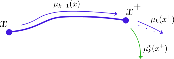
Figure 2: Suboptimal trajectory, visualizing the terms in Assumption 2.

Assumption 2 imposes a contractivity-like condition on the suboptimal policy evaluated on the suboptimal trajectory, as visualized in Figure 2. In words, it implies that the input generated by $\mu$ at time $k$ is closer to the optimal input generated by $\mu^{\star}$ at the same state, compared to the input generated by $\mu$ at the previous timestep $k-1$ and the preceding state. In some cases, the contraction constant, $\eta_{k}$ of the suboptimal policy can be thought of as a design parameter that can be tuned to control the desired level of suboptimality depending on the available computational budget. Gradient descent-based methods where the suboptimal policy performs a finite number of iterations of an optimization problem [25] is a notable case where Assumption 2 holds. We direct the reader to Section 5 for further details on this.

We restrict our attention to systems where the controllable dynamics, $g$, are Lipschitz continuous with respect to $u$ uniformly in $x$ and $k$.

Assumption 3.

There exists a $L_{u}\in\mathbb{R}_{+}$, such that for any $(u,v)\in\mathbb{R}^{m}\times\mathbb{R}^{m}$, for all $x\in\mathcal{D}^{\mu},k\in\mathbb{N}$

$$\|g(k,x,u)-g(k,x,v)\|\leq L_{u}\|u-v\|.$$

This is satisfied, for instance, in linear time-invariant systems or nonlinear systems in certain feedback-linearizable forms (see [26, 27] for details). Finally, we restrict our analysis to local Lipschitz continuous stage costs.

Assumption 4.

(Stage costs). For all $k\in\mathbb{N}$ there exist $M_{x},M_{u}\in\mathbb{R}_{+}$, such that for all $(x,y)\in\mathcal{D}^{\mu}\times\mathcal{D}^{\mu}$ and $(u,z)\in\mathcal{U}\times\mathcal{U}$

$$\|c_{k}(x,u)-c_{k}(y,z)\|\leq M_{x}\|x-y\|+M_{u}\|u-z\|.$$

3 Suboptimality Gap Analysis

In this section, we analyze the suboptimality gap for a given policy, and show that $\mathcal{R}_{T}$ scales with the product of the path length of the suboptimal dynamics and a vector dependent on the contractive constants. We define the backward difference path vector, ${\Delta}\in\mathbb{R}^{T-1}$, to be

$${\Delta}:=\begin{bmatrix}\|\delta x_{1}\|&\|\delta x_{2}\|&\ldots&\|\delta x_{T-1}\|\end{bmatrix}^{\top},$$

where $\delta x_{k}=x_{k}-x_{k-1},\;k\in\mathbb{N}_{+}$, where $x_{k}$ is the state at time $k$ for the suboptimal dynamics (4). The path length of the suboptimal trajectory is then defined as $\mathcal{S}_{T}=\|{\Delta}\|_{1}$ and the Euclidean path length as $\mathcal{S}_{T,2}:=\|{\Delta}\|$.

The policy contraction rate vector, ${\tilde{\eta}}\in\mathbb{R}^{T-1}$ is defined as

$${\tilde{\eta}}:=\begin{bmatrix}\tilde{\eta}_{1}&\tilde{\eta}_{2}&\ldots&\tilde{\eta}_{T-1}\end{bmatrix}^{\top},$$

where

$$\tilde{\eta}_{k}:=\sum_{i=k}^{T-1}\prod_{j=k}^{i}\eta_{j},\qquad\forall k\in[0,T-1].$$

Note that $\tilde{\eta}_{k}=\mathcal{O}(\eta_{k})$ and provides a weighting on the influence of the $\delta x_{k}$ on $\mathcal{R}_{T}$. This is analyzed further in Section 3.2. We denote the Euclidean norm of the suboptimality vector by $\bar{\eta}:=\|{\tilde{\eta}}\|$. The rate of change of the optimal input $\mu^{\star}(x^{\star})$ is captured by the vector $a\in\mathbb{R}_{+}^{T-1}$, defined as

$$a:=\begin{bmatrix}a_{1}&a_{2}&\ldots&a_{T-1}\end{bmatrix}^{\top}.$$

3.1 Upper Bound

The bound in the following theorem captures the tradeoff between suboptimality and the additional cost in closed-loop.

Theorem 1.

Under Assumptions 1, 3 and 4 hold, the suboptimality gap of any policy, $\mu$, satisfying Assumption 2 satisfies

$$\mathcal{R}_{T}^{\mu}(x_{0})=\mathcal{O}\left(\left(a+{\Delta}\right)^{\top}\tilde{\eta}\right),\quad\forall x_{0}\in\mathcal{D}^{\mu}.$$

Specifically, it is bounded by

$$\mathcal{R}_{T}^{\mu}(x_{0})\leq\bar{M}\left(\tilde{\eta}_{0}\|\delta u_{0}\|+\left(a+L{\Delta}\right)^{\top}{\tilde{\eta}}\right),\quad\forall x_{0}\in\mathcal{D}^{\mu},$$

where $\bar{M}:=\left(M_{u}+\frac{\left(M_{u}L+M_{x}\right)C_{w}L_{u}\left(1-\rho^{T}\right)}{1-\rho}\right)$.

The bound in the theorem tends to zero as $\tilde{\eta}$ decreases. This is intuitive, as smaller $\tilde{\eta}$ suggests that the benchmark and suboptimal trajectories are closer to each other. Additionally, the suboptimality gap is a relative measure, but the bound is fully decoupled from the performance of $\mu^{\star}$ and only depends on the performance of the suboptimal state evolution if $a=\boldsymbol{0}$. The above bound can also be represented in terms of the pathlength, $\mathcal{R}_{T}(x_{0})=\mathcal{O}(\bar{\eta}\mathcal{S}_{T,2})$. The path length, $\mathcal{S}_{T,2}$, captures the transient behavior of the suboptimal system and is well-defined in the limit as ${T\rightarrow\infty}$, for example when (4) is exponentially stable.

Before we prove Theorem 1, we introduce the following supporting lemmas. In the subsequent proofs, we make use of the Cauchy Product inequality defined for two finite series $\{a_{i}\}_{i=1}^{T}$ and $\{b_{i}\}_{i=1}^{T}$

$$\textstyle{\sum_{i=0}^{T}\left|\sum_{j=0}^{i}a_{j}b_{i-j}\right|\leq\left(\sum_{i=0}^{T}|a_{i}|\right)\left(\sum_{j=0}^{T}|b_{j}|\right)}.$$ (6)

Lemma 1.

Under Assumption 1, for any policy, $\mu$, satisfying Assumption 2

$$\begin{split}&\sum_{k=0}^{T-1}\|\mu_{k}(x_{k})-\mu_{k}^{\star}(x_{k})\|\\ &\qquad\qquad\qquad\leq\tilde{\eta}_{0}\|\delta u_{0}\|+\left(a+L{\Delta}\right)^{\top}{\tilde{\eta}},\quad\forall x_{0}\in\mathcal{D}^{\mu},\end{split}$$

where $\delta u_{0}:=\nu-\mu^{\star}_{0}(x_{0})$.

Proof.

For all $x_{k}\in\mathcal{D}^{\mu},\;k\in\mathbb{N}_{+}$, define $d_{k}:=\mu_{k}(x_{k})-\mu_{k}^{\star}(x_{k})$. Then

$$\|d_{k}\| \stackrel{{\scriptstyle{(a)}}}{{\leq}}\eta_{k}\|\mu_{k-1}(x_{k-1})-\mu^{\star}_{k}(x_{k})\|$$

$$\begin{split}&\stackrel{{\scriptstyle{(b)}}}{{\leq}}\eta_{k}\|\mu_{k-1}(x_{k-1})-\mu^{\star}_{k-1}(x_{k-1})\|\\ &\qquad\qquad\qquad+\eta_{k}\|\mu^{\star}_{k-1}(x_{k-1})-\mu^{\star}_{k}(x_{k})\|\end{split}$$

$$\begin{split}&\stackrel{{\scriptstyle{(c)}}}{{\leq}}\eta_{k}\|d_{k-1}\|+\eta_{k}\|\mu^{\star}_{k-1}(x_{k-1})-\mu^{\star}_{k-1}(x_{k})\|\\ &\qquad\qquad\qquad+\eta_{k}\|\mu^{\star}_{k-1}(x_{k})-\mu^{\star}_{k}(x_{k})\|\end{split}$$

$$\begin{split}&\stackrel{{\scriptstyle{(d)}}}{{\leq}}\eta_{k}\|d_{k-1}\|+\eta_{k}L\|x_{k}-x_{k-1}\|+\eta_{k}a_{k},\end{split}$$

where the inequality $(a)$ follows directly from Assumption 2, $(b)$ and $(c)$ follow from the triangle inequality for vector norms and $(d)$ from the uniform Lipschitz condition in Assumption 1.i. and Assumption 1.ii.. Applying the above inequality recursively leads to

$$\|d_{k}\| \leq\|d_{0}\|\prod_{i=1}^{k}\eta_{i}+L\sum_{j=1}^{k}\left(a_{j}+L\|\delta x_{j}\|\right)\prod_{i=j}^{k}\eta_{i},$$

for all $k\in\mathbb{N}_{+}$. Summing

$$\begin{split}&\sum_{k=0}^{T-1}\|d_{k}\|\\ &\leq\|d_{0}\|\left(1+\sum_{k=1}^{T-1}\prod_{i=1}^{k}\eta_{i}\right)+L\sum_{k=1}^{T-1}\sum_{j=1}^{k}\left(a_{j}+L\|\delta x_{j}\|\right)\prod_{i=j}^{k}\eta_{i}\end{split}$$

$$\leq\tilde{\eta}_{0}\|\delta u_{0}\|+\sum_{k=1}^{T-1}\sum_{j=1}^{k}\left(a_{j}+L\|\delta x_{j}\|\right)\prod_{i=j}^{k}\eta_{i}$$

$$=\tilde{\eta}_{0}\|\delta u_{0}\|+\left(a+L{\Delta}\right)^{\top}{\tilde{\eta}},$$

where the second inequality follows from Assumption 2, by denoting $\delta u_{0}:=\nu-\mu^{\star}_{0}(x_{0})$, and the equality from the definition of ${\Delta}$ and ${\tilde{\eta}}$. ∎

The following lemma provides an upper bound for the finite-time suboptimality due to trajectory mismatch.

Lemma 2.

Under Assumptions 1 and 3, for any policy, $\mu$, satisfying Assumption 2

$$\sum_{k=0}^{T}\|x_{k}-x^{\star}_{k}\|\leq\|x_{0}-x_{0}^{\star}\|\left(\frac{C_{0}\left(1-\rho^{T}\right)}{1-\rho}\right)$$

$$\qquad+\frac{C_{w}L_{u}\left(1-\rho^{T}\right)}{1-\rho}\left(\tilde{\eta}_{0}\|\delta u_{0}\|+\left(a+L{\Delta}\right)^{\top}{\tilde{\eta}}\right),$$

for all $x_{0},x_{0}^{\star}\in\mathcal{D}^{\mu}$, where $x_{k}$ and $x_{k}^{\star}$ are the states at time $k$ under, respectively, the suboptimal and optimal policies, $\mu$ and $\mu^{\star}$, and $C_{0},C_{W}\in\mathbb{R}_{+}$.

Proof.

Given the boundedness of $\mathcal{U}$, the uniform Lipschitz continuity of $g$ in $u$, and recalling the definition of $w$ from (4), it follows that there exists a $r_{w}\in\mathbb{R}_{+}$, such that $w_{k}(x_{k})\in\mathcal{B}_{r_{w}},k\in\mathbb{N}$. Then, under Assumption 1, and considering (4) to be the perturbed version of the optimal dynamics (3), there exist $C_{0},C_{w}\in\mathbb{R}_{+}$ and $\rho\in(0,1)$, such that for all $k\in\mathbb{N}$ and $x_{0},x_{0}^{\star}\in\mathcal{D}^{\mu}$

$$\|x_{k}-x_{k}^{\star}\| \leq C_{0}\rho^{k}\|x_{0}-x_{0}^{\star}\|+C_{w}\sum_{i=0}^{k-1}\rho^{k-i-1}\|w_{i}(x_{i})\|$$

$$\leq C_{0}\rho^{k}\|x_{0}-x_{0}^{\star}\|+C_{w}L_{u}\sum_{i=0}^{k-1}\rho^{k-i-1}\|d_{i}\|,$$

where the second inequality follows from Assumption 3, by recalling $d_{k}:=\mu_{k}(x_{k})-\mu_{k}^{\star}(x_{k})$. Summing up over the whole trajectory and noting the resultant finite geometric series

$$\sum_{k=0}^{T}\|x_{k}-x^{\star}_{k}\|$$

$$\;\leq\|x_{0}-x_{0}^{\star}\|\left(\frac{C_{0}\left(1-\rho^{T}\right)}{1-\rho}\right)+C_{w}L_{u}\sum_{k=0}^{T-1}\sum_{i=0}^{k}\rho^{k-i}\|d_{i}\|$$

$$\;\leq\|x_{0}-x_{0}^{\star}\|\left(\frac{C_{0}\left(1-\rho^{T}\right)}{1-\rho}\right)+C_{w}L_{u}\sum_{k=0}^{T-1}\rho^{k}\;\sum_{i=0}^{T-1}\|d_{i}\|,$$

where we have used the Cauchy product for the last inequality. Finally, the result follows by using the bound in Lemma 1. ∎

Similarly, the suboptimality due to the difference in applied inputs can be bounded in the following Lemma.

Lemma 3.

Under Assumptions 1 and 3, for any policy, $\mu$, satisfying Assumption 2

$$\sum_{k=0}^{T-1}\|\mu_{k}(x_{k})-\mu_{k}^{\star}(x_{k}^{\star})\|\leq\|x_{0}-x_{0}^{\star}\|\frac{LC_{0}\left(1-\rho^{T}\right)}{1-\rho}$$

$$+\left(\tilde{\eta}_{0}\|\delta u_{0}\|+\left(a+L{\Delta}\right)^{\top}{\tilde{\eta}}\right)\left(1+\frac{LC_{w}L_{u}\left(1-\rho^{T}\right)}{1-\rho}\right),$$

for all $x_{0},x_{0}^{\star}\in\mathcal{D}^{\mu}$, where $x_{k}$ and $x_{k}^{\star}$ are the states at time $k$ under, respectively, the suboptimal and optimal policies, $\mu$ and $\mu^{\star}$, and $C_{0},C_{w}\in\mathbb{R}_{+}$.

Proof.

Using the triangle inequality for vector norms and defining $d_{k}:=\mu_{k}(x_{k})-\mu_{k}^{\star}(x_{k})$

$$\|\mu_{k}(x_{k})-\mu_{k}^{\star}(x_{k}^{\star})\| \leq\|d_{k}\|+\|\mu_{k}^{\star}(x_{k})-\mu_{k}^{\star}(x_{k}^{\star})\|$$

$$\leq\|d_{k}\|+L\|x_{k}-x_{k}^{\star}\|,$$

where the last inequality follows from Lipschitz continuity of $\mu^{\star}$ from Assumption 1.i.. Summing up over the trajectory horizon and using the results from Lemmas 1 and 2 completes the proof. ∎

Proof of Theorem 1.

By Assumption 4, for all $x_{0},x_{0}^{\star}\in\mathcal{D}^{\mu}$

$$\mathcal{R}_{T}(x_{0},x_{0}^{\star}):=J_{T}(x_{0},{\mu})-J_{T}(x_{0}^{\star},\mu^{\star})$$

$$\qquad\leq M_{x}\sum_{k=0}^{T}\|x_{k}-x_{k}^{\star}\|-M_{u}\sum_{k=0}^{T}\|\mu_{k}(x_{k})-\mu_{k}^{\star}(x_{k}^{\star})\|.$$

Then, using Lemmas 2 and 3 for the two respective sums

$$\mathcal{R}_{T}(x_{0},x_{0}^{\star}) \leq\|x_{0}-x_{0}^{\star}\|\left(M_{u}L+M_{x}\right)\left(\frac{C_{0}\left(1-\rho^{T}\right)}{1-\rho}\right)$$

$$\qquad+\bar{M}\left(\tilde{\eta}_{0}\|\delta u_{0}\|+\left(a+L{\Delta}\right)^{\top}{\tilde{\eta}}\right).$$

The result follows by taking $x_{0}=x_{0}^{\star}$. ∎

For the special case when the contraction rate of the suboptimal policy is constant, the bound in Theorem 1 can be simplified.

Corollary 1.

Under Assumptions 1, 3 and 4, the suboptimality gap of any policy, $\mu$, satisfying Assumption 2 with $\eta_{k}=\eta,\;k\in\mathbb{N}$, satisfies

$$\mathcal{R}_{T}^{\mu}(x_{0})=\mathcal{O}\left(\eta\left(\mathcal{S}_{T}+\|a\|_{1}\right)\right),\quad\forall x_{0}\in\mathcal{D}^{\mu}.$$

Proof.

In the special case when $\eta_{k}=\eta,k\in\mathbb{N}$, $\tilde{\eta}_{k}=\eta\left(1-\eta^{T-k+1}\right)/\left(1-\eta\right),\;k\in[0,T]$ and is bounded by

$$\tilde{\eta}_{k}\leq\frac{\eta}{1-\eta},\quad k\in[0,T].$$

The complexity term then satisfies

$$\left(a+{\Delta}\right)^{\top}{\tilde{\eta}}\leq\frac{\eta\left(\mathcal{S}_{T}+\|a\|_{1}\right)}{1-\eta}.$$

The rest of the proof follows directly from Theorem 1 by replacing the complexity term with the new bound. ∎

3.2 Interpretation of the Upper Bound

The term $\tilde{\eta}_{0}\|\delta u_{0}\|$ in the bound of Theorem 1 captures the error due to the initial mismatch in the control input, $\delta u_{0}$. This term in general cannot be avoided, unless the initial “guess” of the input $\nu$ is correct, or $\eta_{0}=0$, so that the suboptimal and optimal policies match at the initial timestep.

The second term, $a^{\top}\tilde{\eta}$, scales with the magnitude of the rate of change of the time-varying benchmark policy $\mu^{\star}$, as defined in Assumption 1.ii.. It vanishes either when $\mu^{\star}$ is stationary, or when the benchmark and suboptimal policies coincide.

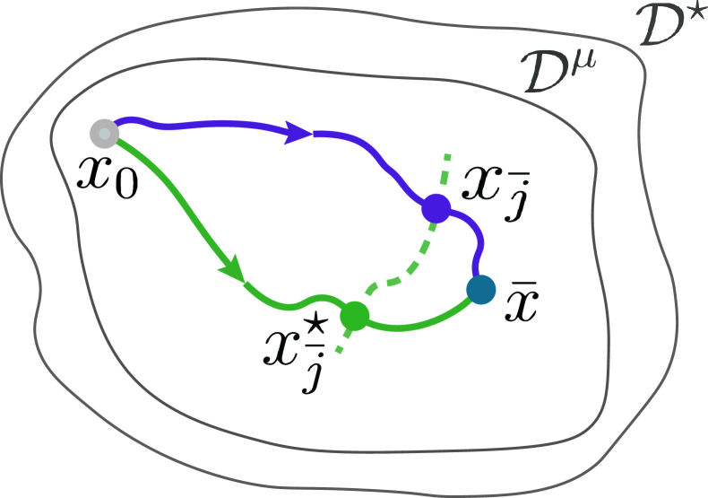
(a) Exponentially stable case. Suboptimality is captured by (7).

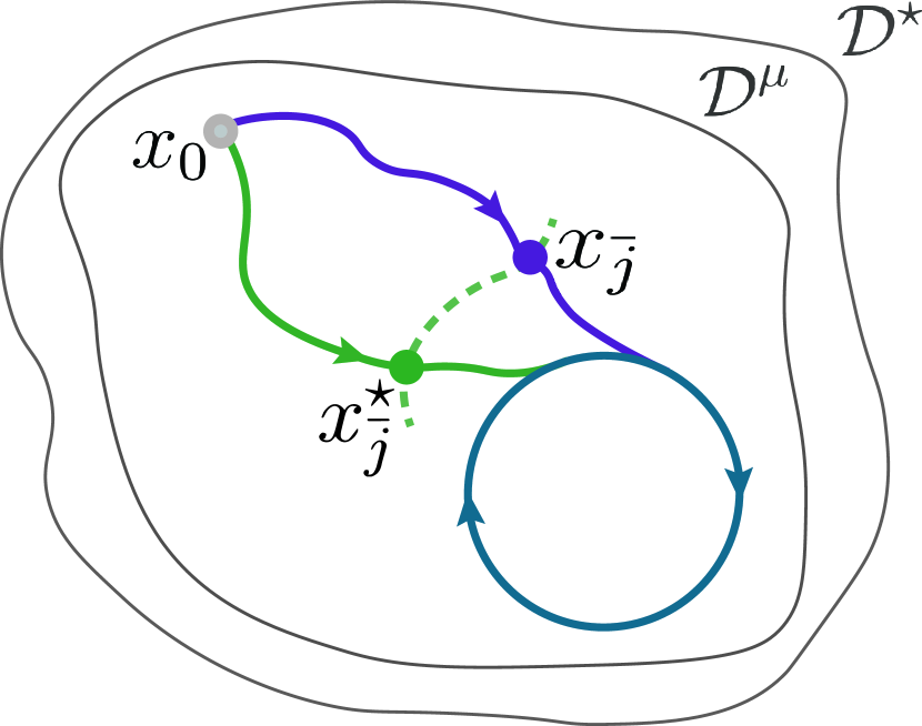
(b) Case of limit cycles. Suboptimality is captured by (8).

Figure 3: The pictorial evolution of suboptimal (in blue) and optimal (in green) trajectories evolving in $\mathcal{D}^{\mu}\subseteq\mathcal{D}^{\star}$.

The main complexity term of interest is the last one. This captures the suboptimality of the policy through the inner product of the path vector ${\Delta}$ and the suboptimality vector ${\tilde{\eta}}$. To study the interplay of these two quantities in more detail, let us consider the case when the benchmark dynamics, (3) under the policy $\mu^{\star}$ have an equilibrium at some $\bar{x}\in\mathbb{R}^{n}$. If the suboptimal policy makes the closed-loop (4) exponentially stable with $\eta_{k}\neq 0,\;\forall k\in\mathbb{N}$, then the backward difference vector norm $\|\delta x_{j}\|\approx 0,\;\forall j\geq\bar{j}$, for some $\bar{j}\in\mathbb{N}$, as visualised in Figure 3(a). In such a setting, the finite value of the suboptimality gap is captured by the complexity term as

$$\begin{split}&{\Delta}^{\top}{\tilde{\eta}}=\\ &\left[\begin{array}[]{c c|c c c}\|\delta x_{1}\|\;\ldots\;\color[rgb]{.5,.5,.5}\makebox[0.0pt][l]{$\smash{\underbrace{\phantom{\begin{matrix}\color[rgb]{.5,.5,.5}\|\delta x_{\bar{j}}\|\;\color[rgb]{.5,.5,.5}\ldots\;\color[rgb]{.5,.5,.5}\|\delta x_{T-1}\|\end{matrix}}}_{\text{$\approx\boldsymbol{0}$}}}$}\color[rgb]{.5,.5,.5}\|\delta x_{\bar{j}}\|\;\color[rgb]{.5,.5,.5}\ldots\;\color[rgb]{.5,.5,.5}\|\delta x_{T-1}\|\end{array}\right]\left[\begin{array}[]{c}\vphantom{\vdots}\tilde{\eta}_{1}\\ \vphantom{\vdots}\vdots\\ \hline\cr\vphantom{\vdots}\tilde{\eta}_{\bar{j}}\\ \vphantom{\vdots}\vdots\\ \vphantom{\vdots}\tilde{\eta}_{T-1}\end{array}\right]\begin{array}[]{@{\kern-\nulldelimiterspace}l@{}}1.2pt\lx@intercol\begin{array}[]{@{}c@{}}\vphantom{\vdots}\\ \vphantom{\vdots}\end{array}\\ 1.2pt\lx@intercol\left.\begin{array}[]{@{}c@{}}\vphantom{\vdots}\\ \vphantom{\vdots}\\ \vphantom{\vdots}\\ \end{array}\right\}\neq 0\end{array}.\end{split}$$ (7)

This example coincides with the suboptimal LQMPC use case discussed in detail in Section 5. Among other possibilities, one can also consider the case when the benchmark dynamics (3) converge to a limit cycle. Since (3) is E-$\delta$-ISS it follows from (4) that if at a given point in time $\bar{j}\in\mathbb{N}$, the suboptimal policy becomes optimal, i.e. $\eta_{j}=0,\;\forall j\geq\bar{j}$, then the trajectories will necessarily coincide, as visualised in Figure 3(b). This is captured by the complexity term as

$$\begin{split}&{\Delta}^{\top}{\tilde{\eta}}=\\ &\left[\begin{array}[]{c c|c c c}\|\delta x_{1}\|\;\ldots\;\makebox[0.0pt][l]{$\smash{\underbrace{\phantom{\begin{matrix}\|\delta x_{\bar{j}}\|\;\ldots\;\|\delta x_{T-1}\|\end{matrix}}}_{\text{$\neq\boldsymbol{0}$}}}$}\|\delta x_{\bar{j}}\|\;\ldots\;\|\delta x_{T-1}\|\end{array}\right]\left[\begin{array}[]{c}\vphantom{\vdots}\tilde{\eta}_{1}\\ \vphantom{\vdots}\vdots\\ \hline\cr\color[rgb]{.5,.5,.5}\vphantom{\vdots}\tilde{\eta}_{\bar{j}}\\ \color[rgb]{.5,.5,.5}\vphantom{\vdots}\vdots\\ \color[rgb]{.5,.5,.5}\vphantom{\vdots}\tilde{\eta}_{T-1}\end{array}\right]\color[rgb]{.5,.5,.5}\begin{array}[]{@{\kern-\nulldelimiterspace}l@{}}1.2pt\lx@intercol\begin{array}[]{@{}c@{}}\vphantom{\vdots}\\ \vphantom{\vdots}\end{array}\\ 1.2pt\lx@intercol\left.\begin{array}[]{@{}c@{}}\vphantom{\vdots}\\ \vphantom{\vdots}\\ \vphantom{\vdots}\\ \end{array}\right\}\approx\boldsymbol{0}\end{array}\color[rgb]{0,0,0}{.}\end{split}$$ (8)

Even though the path length keeps increasing, the norm of the suboptimality vector is finite, resulting in a finite suboptimality gap, containing only the additional cost due to suboptimality at the first $\bar{j}$ timesteps.

4 Exponentially Stable Policies and E-$\delta$-ISS

In this section, we analyze the E-$\delta$-ISS property of the closed-loop system (3), and derive conditions under which the exponential stability of a nonlinear system implies E-$\delta$-ISS for non-smooth dynamics.

We treat (3) as a general nonlinear time-varying system of the form

$$x_{k+1}=f(k,x_{k}),\quad\forall k\in\mathbb{N},$$ (9)

where $f:\mathbb{N}\times\mathcal{D}\rightarrow\mathcal{D}$ is continuous with respect to both arguments and $x_{k_{0}}=\xi\in\mathbb{R}^{n}$ for some $k_{0}\in\mathbb{N}$ and $\mathcal{D}\subseteq\mathbb{R}^{n}$. Note that by definition of $f$, $\mathcal{D}$ is forward invariant. The solution of the system (9) at time $k\geq k_{0},\;k_{0}\in\mathbb{N}$ is characterized by the function $\phi:\mathbb{N}\times\mathbb{N}\times\mathcal{D}\rightarrow\mathcal{D}$ mapping the current time, initial time and the initial state to the current state, i.e. $\phi(k+1,k_{0},\xi)=f(k,\phi(k,k_{0},\xi))$ for all $k\geq k_{0}\;k_{0}\in\mathbb{N}$. We consider the origin to be an equilibrium point for (9), i.e. $f(k,\boldsymbol{0})=\boldsymbol{0}$ for all $k\geq k_{0}$. Although this restricts the attention to regulation problems, one can convert a tracking problem into a regulation one given the form of the system (1). We impose the following assumption.

Assumption 5.

(Local Behavior)

1. The dynamics (9) are $L_{f}$-Lipschitz continuous in $\mathcal{D}$,

2. $\mathcal{D}$ is compact,

3. There exists a forward invariant region $\mathcal{D}_{0}\subseteq\mathcal{D}$ containing the origin, such that in $\mathcal{D}_{0}$, the dynamics (9) are continuously differentiable with respect to $x$ and the Jacobian matrix $[\partial f/\partial x]$ is bounded and Lipschitz.

Remark 1.

The conditions on the Jacobian matrix of $f$ in Assumption 5 are required only in the time-varying case [26].

Before presenting the main results of this section, we present a series of auxiliary definitions and theorems for (incremental) exponential stability, for completeness.

4.1 Preliminaries on Exponential Stability

We formally define uniform exponential stability for discrete-time, nonlinear time-varying systems [27].

Definition 2.

Given the system, (9), the equilibrium point $x=\boldsymbol{0}$ is said to be uniformly locally exponentially stable with a rate $\lambda$, in a ROA $\mathcal{D}\subseteq\mathbb{R}^{n}$, if there exist constants $d\in R_{+}$ and $\lambda\in(0,1)$, such that

$$\|\phi(k,k_{0},\xi)\|\leq d\|\xi\|\lambda^{k},\quad\forall\;\xi\in\mathcal{D},\;k_{0}\in\mathbb{N}.$$ (10)

If (10) holds for all initial states $\xi\in\mathbb{R}^{n}$, then the equilibrium is uniformly globally exponentially stable.

If the origin is locally/globally exponentially stable, we also refer to the system (9) as such. Lyapunov theory provides necessary and sufficient conditions for the exponential stability of nonlinear systems. Below are the discrete-time Lyapunov theorems for exponential stability.

Theorem 2.

[27, Thm. 13.11] Consider the nonlinear system (9) and assume that there exists a continuous mapping $V:\mathbb{N}\times\mathcal{D}\rightarrow\mathbb{R}_{+}$. If there exist constants $c_{1},c_{2}\in\mathbb{R}_{+}$, $\beta\in(0,1)$ and $p\geq 1$, such that

$$c_{1}\|x\|^{p}\leq V(k,x)\leq c_{2}\|x\|^{p},\qquad \forall x\in\mathcal{D},\;k\in\mathbb{N},$$

$$V\left(k+1,f(k,x)\right)\leq\beta^{p}V(k,x),\qquad \forall x\in\mathcal{D},\;k\in\mathbb{N},$$

then the nonlinear system (9) is uniformly locally exponentially stable in $\mathcal{D}$, with rate $\beta$.

The converse Lyapunov theorem for the discrete-time case shows the implication in the opposite direction.

Theorem 3.

[28, Thm. 2] If the nonlinear system (9) is uniformly locally exponentially stable in $\mathcal{D}$, then there exists a continuous function $V:\mathbb{N}\times\mathcal{D}\rightarrow\mathbb{R}$ and constants $c_{1},c_{2}\in\mathbb{R}_{+}$ and $\beta\in(0,1)$, such that

$$c_{1}\|x\|^{2}\leq V(k,x)\leq c_{2}\|x\|^{2},\qquad \forall x\in\mathcal{D},\;k\in\mathbb{N}$$ (11)

$$V\left(k+1,f(k,x)\right)\leq\beta^{2}V(k,x),\qquad \forall x\in\mathcal{D},\;k\in\mathbb{N}.$$ (12)

The above theorems generalize to uniform global exponential stability if $\mathcal{D}=\mathbb{R}^{n}$ [26, 29]. In continuous-time, the rate of change of the Lyapunov function with respect to the state is bounded by the norm of the state [26, Thm 4.14]. The following Lemma is the discrete-time equivalent of this bound.

Lemma 4.

Under Assumption 5.i., if (9) is uniformly locally exponentially stable, then there exists a continuous Lyapunov function $V:\mathbb{N}\times\mathcal{D}\rightarrow\mathbb{R}$, that, in addition to (11) and (12), satisfies

$$|V(k,x)-V(k,y)|\leq c_{3}\|x-y\|\left(\|x\|+\|y\|\right),\quad\forall k\in\mathbb{N},$$

for all $x,y\in\mathcal{D}$, and some $c_{3}\in\mathbb{R}_{+}$.

The proof of Lemma 4 is provided in the appendix.

When the system is linear time-varying, the Lyapunov function has a quadratic structure.

Theorem 4.

[30, Thm. 23.3] The linear time-varying system

$$x_{k+1}=A(k)x_{k},\qquad k\in\mathbb{N}$$

is uniformly exponentially stable, if and only if there exists a sequence of positive-definite, bounded matrices $P(k)\in\mathbb{R}^{n\times n}$, $k\in\mathbb{N}$, satisfying the following difference Lyapunov equation

$$A^{\top}(k)P(k+1)A(k)-P(k)\leq-cI,$$ (13)

for some $c\in\mathbb{R}_{+}$.

4.2 Preliminaries on Exponential Incremental Stability

Exponential incremental stability shows the exponential convergence of two trajectories generated by the same system to each other [15, 17].

Definition 3.

The nonlinear system (9) is uniformly semiglobally exponentially incrementally stable in $\mathcal{D}$ if there exists a $d\in\mathbb{R}_{+}$ and $\lambda\in(0,1)$, such that for all initial states $\xi,\zeta\in\mathcal{D}$ and for all $k\geq k_{0},\;k_{0}\in\mathbb{N}$

$$\|\phi(k,k_{0},\xi)-\phi(k,k_{0},\zeta)\|\leq d\|\xi-\zeta\|\lambda^{k}.$$

In the case $\mathcal{D}=\mathbb{R}^{n}$, the system is said to be uniformly globally exponentially incrementally stable.

The theory of exponential convergence of two trajectories of the same system has first been studied as uniform convergence by Demidovich [24, 31], and later extended through contraction theory [16, 17]. Contraction is a sufficient condition for exponential incremental stability, that when $f$ is smooth, can be checked by the following condition.

Theorem 5.

[17, Thm 2.8] Under Assumption 5.iii., suppose there exists a uniform positive definite matrix $P(k)$ and a positive scalar $\rho\in(0,1)$, such that

$$D(k,x):=\frac{\partial f}{\partial x}(k,x)^{T}P(k+1)\frac{\partial f}{\partial x}(k,x)-\rho^{2}P(k)$$ (14)

is negative definite uniformly for all $\xi\in\mathcal{D}_{0}$. Then (9) is uniformly semiglobally exponentially incrementally stable in $\mathcal{D}_{0}$ with a rate of $\rho$.

We also state the following converse Lyapunov theorem. The proof, extended from [14] and [15], is provided in the appendix.

Theorem 6.

If the system (9) is uniformly semiglobally exponentially incrementally stable in $\mathcal{D}$, then there exists a function $V:\mathbb{N}\times\mathcal{D}\times\mathcal{D}\rightarrow\mathbb{R}_{+}$ and constants $c_{1},c_{2}\in\mathbb{R}_{+}$ and $\beta\in(0,1)$, such that for all $x,y\in\mathcal{D}$ and $k\in\mathbb{N}$

$$c_{1}\|x-y\|^{2}\leq V(k,x,y)\leq c_{2}\|x-y\|^{2},$$ (15)

$$V\left(k+1,f(k,x),f(k,y)\right)\leq\beta^{2}V(k,x,y).$$ (16)

Moreover, under Assumption 5.i., there exists a constant $c_{3}\in\mathbb{R}_{+}$, such that for all $x,y,\tilde{x},\tilde{y}\in\mathcal{D}$ and $k\in\mathbb{N}$

$$\begin{split}&|V(k,x,y)-V(k,\tilde{x},\tilde{y})|\leq\\ &\leq c_{3}\left(\|x-\tilde{x}\|+\|y-\tilde{y}\|\right)\left(\|x-y\|+\|\tilde{x}-\tilde{y}\|\right).\end{split}$$ (17)

4.3 Main Results

In this subsection we show that if the nonlinear dynamics (9) are uniformly locally exponentially stable in a given forward invariant region and satisfy Assumption 5, then they are also E-$\delta$-ISS in the same region. First we show that under the local Lipschitz continuity assumption, exponential incremental stability implies E-$\delta$-ISS.

Theorem 7.

Under Assumptions 5.i. and 5.ii., if the nonlinear system (9) is uniformly semigobally exponentially incrementally stable in $\mathcal{D}$, then it is E-$\delta$-ISS in the same region.

Proof.

Given the nonlinear system (9), consider the evolution of two, respectively unperturbed and perturbed trajectories

$$x_{k+1} =f(k,x_{k}),$$

$$y_{k+1} =f(k,y_{k})+w_{k},$$

for some $x_{0},y_{0}\in\mathcal{D}$, where $w_{k}\in\mathcal{B}_{r_{w}}$, for some $r_{w}\in\mathbb{R}_{+}$ is such that $y_{k}\in\mathcal{D}$ for all $k\in\mathbb{N}$. Given $f$ is uniformly semiglobally exponentially incrementally stable in $\mathcal{D}$, then from Theorem 6, there exists a Lyapunov function $V:\mathbb{N}\times\mathcal{D}\times\mathcal{D}\rightarrow\mathbb{R}_{+}$ satisfying (15)-(17). Then, for any $x,y\in\mathcal{D}$, and $w\in\mathcal{B}_{r_{w}}$

$$\begin{split}&V\left(k+1,f(k,x),f(k,y)+w\right)-V\left(k,x,y\right)=\end{split}$$

$$\begin{split}&=V\left(k+1,f(k,x),f(k,y)\right)-V\left(k,x,y\right)\\ &+V\left(k+1,f(k,x),f(k,y)+w\right)-V\left(k+1,f(k,x),f(k,y)\right)\end{split}$$

$$\begin{split}&\leq-\left(1-\beta^{2}\right)c_{1}\|x-y\|^{2}\\ &\quad+c_{3}\|w\|\left(\|f(k,x)-f(k,y)-w\|+\|f(k,x)-f(k,y)\|\right)\\ &\leq-\left(1-\beta^{2}\right)c_{1}\|x-y\|^{2}+c_{3}\|w\|^{2}+2c_{3}\|w\|\|x-y\|,\end{split}$$

where the first inequality follows from Theorem 6, and the second from the triangle inequality. Completing the square, and denoting $c_{4}:=(1-\beta^{2})c_{1}$ it follows from above that

$$\begin{split}&V\left(k+1,f(k,x),f(k,y)\right)-V\left(k,x,y\right)\leq\end{split}$$

$$\begin{split}&\leq\frac{-3c_{4}}{2}\|x-y\|^{2}\\ &\qquad\qquad+\left(\frac{\sqrt{c_{4}}}{\sqrt{2}}\|x-y\|+\frac{c_{3}\sqrt{2}\|w\|}{\sqrt{c_{4}}}\right)^{2}-\frac{2c_{3}^{2}\|w\|^{2}}{c_{4}}\end{split}$$

$$\begin{split}&\leq-\frac{c_{4}}{2}\|x-y\|^{2}+\frac{2c_{3}\|w\|^{2}}{c_{4}^{2}}\leq-\frac{c_{4}}{2c_{2}}V(k,x,y)+\frac{2c_{3}^{2}\|w\|^{2}}{c_{4}},\end{split}$$

where the second inequality follows by the fact that $\left(a^{2}+b^{2}\right)\leq 2a^{2}+2b^{2}$ for any $a,b\in\mathbb{R}$, and the last inequality from Theorem 6. Finally, rearranging the Lyapunov equations it follows that

$$V\left(k+1,f(k,x),f(k,y)\right)\leq\rho^{2}V\left(k,x,y\right)+c_{5}\|w\|^{2},$$

for all $k\in\mathbb{N}$, with $\rho^{2}:=1-\frac{c_{4}}{c_{2}}\in(0,1)$, since $c_{2}>c_{4}$, and $c_{5}:=\frac{2c_{3}^{2}}{c_{4}}$. Unrolling the recursion and using (15)

$$c_{1}\|x_{k}-y_{k}\|^{2} \leq\rho^{2k}V(0,x_{0},y_{0})+c_{5}\sum_{i=0}^{k-1}\rho^{2(k-i-1)}\|w_{i}\|^{2}$$

$$\leq c_{2}\rho^{2k}\|x_{0}-y_{0}\|^{2}+c_{5}\sum_{i=0}^{k-1}\rho^{2(k-i-1)}\|w_{i}\|^{2}.$$

Dividing by $c_{1}$ and taking the square root, completes the proof

$$\|x_{k}-y_{k}\|\leq\sqrt{\frac{c_{2}}{c_{1}}}\rho^{k}\|x_{0}-y_{0}\|+\sqrt{\frac{c_{5}}{c_{1}}}\sum_{i=0}^{k-1}\rho^{k-i-1}\|w_{i}\|.$$

∎

Next we show, that if the following theorem states that if in addition to local Lipschitz continuity, the nonlinear dynamics are also locally differentiable in some arbitrarily small region, $\mathcal{D}_{0}$, around the equilbrium, then uniform local exponential stability implies uniform semiglobal exponential incremental stability and E-$\delta$-ISS by Corollary 2.

Theorem 8.

Under Assumption 5, if the nonlinear system (9) is uniformly locally exponentially stable in $\mathcal{D}$, then it is also uniformly semiglobally exponentially incrementally stable in the same region.

Proof.

We start by showing that the exponential stability of $f$ implies that the linearized dynamics around the origin are also stable by following similar arguments to [26]. Let

$$A(k):=\frac{\partial f(k,x)}{\partial x}(k,\boldsymbol{0}),$$

which is well-defined given Assumption 5. Moreover, there exists a $\bar{A}\in\mathbb{R}_{+}$, such that $\|{A}(k)\|\leq\bar{A}$, $k\in\mathbb{N}$. It follows from Theorem 3, that there exists a continuous mapping $V:\mathbb{N}\times\mathcal{D}\rightarrow\mathbb{R}$ satisfying (11)-(12). Let us consider $V$ as a candidate Lyapunov function for $A(k)$, then for all $x\in\mathcal{D}$, $k\in\mathbb{N}$ there exist constants $\beta\in(0,1)$, $c_{4},d\in\mathbb{R}_{+}$ such that

$$V(k+1,A(k)x)=$$

$$V(k+1,f(k,x))+\left[V(k+1,A(k)x)-V(k+1,f(k,x))\right]$$

$$\leq\beta^{2}V(k,x)+\left[V(k+1,A(k)x)-V(k+1,f(k,x))\right]$$

$$\leq\beta^{2}V(k,x)+c_{4}\|f(k,x)-A(k)x\|\left[f(k,x)+A(k)x\right]$$

$$\leq\beta^{2}V(k,x)+c_{4}\|x\|\cdot\|f(k,x)-A(k)x\|\left(d\beta+\|A(k)\|\right),$$

where the first inequality follows from Theorem 3, the second from Lemma 4 and the last from Definition 2 and properties of induced norms. Denoting $g(k,x):=f(k,x)-A(k)x$, it follows from the Lipschitz continuity of the Jacobian of $f$ [26, Chpt. 4.6] that there exists a $L\in\mathbb{R}_{+}$, such that $\|g(k,x)\|\leq L\|x\|^{2}$, $k\in\mathbb{N}$. Using this

$$V(k+1,A(k)x)\leq\beta^{2}V(k,x)+c_{4}L\left(d\beta+\bar{A}\right)\|x\|^{3}$$

$$\leq\left(\beta^{2}+\frac{c_{4}L\left(d\beta+\bar{A}\right)}{c_{1}}\|x\|\right)V(k,x):=\gamma V(k,x),$$

where the second inequality follows from the converse Lyapunov Theorem 3 for some $c_{1}\in\mathbb{R}_{+}$. Defining $r_{1}:=\min\left\{\frac{c_{1}\left(1-\beta^{2}\right)}{c_{4}L\left(d\beta+\|A\|\right)},\max\limits_{r\in\mathbb{R}_{+}}\left\{\|x\|<r|x\in\mathcal{D}_{0}\right\}\right\}$, for all $\|x\|\leq r_{1}$, it holds that $\gamma<1$. Hence, using Theorem 2 the linearized dynamics $x_{k+1}=A(k)x_{k}$ are uniformly locally exponentially stable. Then, by Theorem 4 there exists a sequence of uniformly positive definite $P(k)$ that solves the difference Lyapunov equation (13) for some $c\in\mathbb{R}_{+}$.

Considering now equation (14), for any $k\in\mathbb{N}$ and $\bar{x}\in\mathcal{D}_{0}$ if we denote $d_{k}(\bar{x}):=\frac{\partial f}{\partial x}(k,\bar{x})-A(k)$ then

$$\frac{\partial f}{\partial x}(k,\bar{x})^{\top}P(k+1)\frac{\partial f}{\partial x}(k,\bar{x})-P(k)$$

$$=\left[A(k)+d_{k}(\bar{x})\right]^{\top}P(k+1)\left[A(k)+d_{k}(\bar{x})\right]-P(k)$$

$$=A(k)^{\top}P(k+1)A(k)-P(k)$$

$$+A(k)^{\top}P(k+1)d_{k}(\bar{x})+d_{k}(\bar{x})^{\top}P(k+1)\left[A(k)+d_{k}(\bar{x})\right]$$

$$\leq-cI+A(k)^{\top}P(k+1)d_{k}(\bar{x})$$

$$\qquad\qquad+d_{k}(\bar{x})^{\top}P(k+1)\left[A(k)+d_{k}(\bar{x})\right],$$

where the first equality follows from the definition of $d_{k}(\bar{x})$ and the last one from Theorem 4.

Following the same arguments as in [26, Chpt. 4.6], there exists a $L_{2}\in\mathbb{R}_{+}$, such that for all $k\in\mathbb{N}$ and $\bar{x}\in\mathcal{D}_{0}$, $\|d_{k}(\bar{x})\|\leq L_{2}\|\bar{x}\|$. Pre- and post-multiplying the above with some $x^{\top}$ and $x$, respectively then yields

$$x^{\top}\left[\frac{\partial f}{\partial x}(k,\bar{x})^{\top}P(k+1)\frac{\partial f}{\partial x}(k,\bar{x})-P(k)\right]x\leq$$

$$-c\|x\|^{2}+2\|x\|^{2}\|A(k)^{\top}P(k+1)d_{k}(\bar{x})\|$$

$$\qquad\qquad+\|x\|^{2}\|d_{k}(\bar{x})^{\top}P(k+1)d_{k}(\bar{x})\|$$

$$\leq-\|x\|^{2}\left(c-2\bar{A}\bar{P}L_{2}\|x\|-\bar{P}r_{d}L_{2}^{2}\|x\|\right),$$

where $r_{d}=\max\limits_{x\in\mathcal{D}}\|x\|$, and $\|P(k)\|\leq\bar{P},\;k\in\mathbb{N}$. Note that the rate of exponential stability of the linear system $A(k)$ is $\sqrt{1-\frac{c}{\bar{P}}}\in(0,1)$. Then, choosing $\rho^{2}>1-\frac{c}{\bar{P}}$, adding $x^{\top}\left(1-\rho^{2}\right)P(k)x$ to both sides of the above inequality and defining $r_{2}:=\frac{c-\left(1-\rho^{2}\right)\bar{P}}{2\bar{A}\bar{P}L_{2}+\bar{P}r_{d}L_{2}^{2}}$ ensures that

$$x^{\top}\left[\frac{\partial f}{\partial x}(k,x)^{T}P(k+1)\frac{\partial f}{\partial x}(k,x)-\rho^{2}P(k)\right]x<0,$$

uniformly in $k$ and $x$, for all $\|x\|<r:=\min\left(r_{1},r_{2}\right)$. This implies by Theorem 5 that for all $\|x\|<r$ the system (9) is uniformly semiglobally exponentially incrementally stable with rate of $\rho$.

To show that the system is also uniformly semiglobally exponentially incrementally stable in $\mathcal{D}$, consider any $\xi_{1},\xi_{2}\in\mathcal{D}$, then for all $k\in\mathbb{N}$, and some $d\in\mathbb{R}_{+}$, the following two inequalities hold

$$\begin{split}&\|\phi(k,k_{0},\xi_{1})-\phi(k,k_{0},\xi_{2})\|\leq\|\phi(k,k_{0},\xi_{1})\|\\ &+\|\phi(k,\xi_{2})\|\leq 2r_{d}d\beta^{k},\end{split}$$ (18)

$$\|\phi(k,k_{0},\xi_{1})-\phi(k,k_{0},\xi_{2})\|\leq L^{k}\underbrace{\|\xi_{1}-\xi_{2}\|}_{:=\Delta\xi}.$$ (19)

The bound in (18) follows from the exponential stability of $f$, and the one in (19) from its Lipschitz continuity. Combining the two

$$\|\phi(k,k_{0},\xi_{1})-\phi(k,k_{0},\xi_{2})\|\leq\min\{2r_{d}d\cdot\beta^{k},L^{k}\|\Delta\xi\|\}.$$

Define $k^{\prime}>0$ such that both $\|\phi(k^{\prime},k_{0},\xi_{1})\|<r,\|\phi(k^{\prime},k_{0},\xi_{2})\|<r$. Then, from the above analysis, there exists a $d^{\prime}\in\mathbb{R}_{+}$, such that for all $k\geq k^{\prime}$ for all $k\geq k^{\prime}$

$$\|\phi(k,k_{0},\xi_{1})-\phi(k,k_{0},\xi_{2})\|$$

$$\leq d^{\prime}\rho^{k-k^{\prime}}\cdot\|\phi(k^{\prime},k_{0},\xi_{1})-\phi(k^{\prime},k_{0},\xi_{2})\|.$$

It then follows that

$$\|\phi(k,k_{0},\xi_{1})-\phi(k,k_{0},\xi_{2})\|\leq d^{\prime}\rho^{k-k^{\prime}}\cdot\min\{r_{d}d\cdot\beta^{k},L^{k}\|\Delta\xi\|\}.$$

Note that for all $k\leq k^{\prime}$

$$\|\phi(k,k_{0},\xi_{1})-\phi(k,k_{0},\xi_{2})\|\leq c\|\Delta\xi\|\rho^{k},$$

where

$$c=\min\Biggl{\{}\left(\frac{\beta}{\rho}\right)^{k^{\prime}}\frac{d_{\mathcal{D}}d}{\|\Delta\xi\|},\left(\frac{L}{\rho}\right)^{k^{\prime}}\Biggr{\}},$$

where $c$ is a constant independent of $\|\Delta\xi\|$ since $k^{\prime}$ is finite and also independent of it. Combining the bounds

$$\|\phi(k,\xi_{1})-\phi(k,\xi_{2})\|\leq cd^{\prime}\rho^{k}\|\Delta\xi\|,\;\;\forall k>0,$$

which is the definition of uniform semiglobal exponential incremental stability. ∎

Combining Theorems 7 and 8 the following corollary follows directly.

Corollary 2.

Under Assumption 5, if the nonlinear system (9) is uniformly locally exponentially stable in $\mathcal{D}$, then it is also E-$\delta$-ISS in the same region.

In the sequel we use these insights to address the closed-loop dynamics under a specific, notable policies.

5 Model Predictive Control - A Use Case

In Section 3 we showed that under certain assumptions on the suboptimal policy $\mu$ (Assumption 2) and the benchmark policy $\mu^{\star}$ (Assumption 1), the suboptimality gap of $\mu$ can be bounded for a certain family of costs. A key condition on the benchmark policy is that of E-$\delta$-ISS. We now exploit the results of Section IV to study the case of linear quadratic MPC.

Consider the control of linear time-invariant dynamical systems, modeled by

$$x_{k+1}=Ax_{k}+Bu_{k},\quad\forall k\in\mathbb{N},$$

where $A\in\mathbb{R}^{n\times n}$, and $B\in\mathbb{R}^{n\times m}$ are the known system matrices. We consider the finite horizon linear quadratic regulator (LQR) whose objective is to minimize the finite-time quadratic cost

$$J_{T}(x_{0},\boldsymbol{u})=\|x_{T}\|^{2}_{P}+\sum_{k=0}^{T-1}\|x_{k}\|^{2}_{Q}+\|u_{k}\|^{2}_{R},$$ (20)

where $Q\in\mathbb{R}^{n\times n}$ and $R\in\mathbb{R}^{m\times m}$ are design matrices and $P$ is taken to be the solution of the discrete Algebraic Riccati Equation, $P=Q+K^{\top}RK+(A-BK)^{\top}P(A-BK)$, with $K=(R+B^{\top}PB)^{-1}(B^{\top}PA)$, and the control inputs must satisfy $u_{k}\in\mathcal{U}$ for all $k>0$, where $\mathcal{U}\subseteq\mathbb{R}^{m}$ is a constraint set. The following standard assumptions ensure a unique minimizer for (20) always exists [32].

Assumption 6.

(Well posed problem)

1. The pair $(A,B)$ is stabilizable, $Q\succ 0$, $R\succ 0$.

2. The input constraint set $\mathcal{U}$ is compact, convex, and contains the origin.

The model predictive controller solves this problem in a receding horizon fashion, solving the following parametric optimal control problem (POCP) at each timestep $k$, having measured a state $x\in\mathbb{R}^{n}$

$$\begin{split}\mu^{\star}(x):=&\operatorname*{arg\,min}_{\boldsymbol{\nu}}\;J_{N}(\xi_{0},\boldsymbol{\nu})\\ \text{s.t.}\;&\xi_{i+1}=A\xi_{i}+B\nu_{i},\;i\!=\!0,\dots,N-1,\\ &\xi_{0}=x,\;\nu_{i}\in\mathcal{U},\;i\!=\!0,\dots,N-1.\end{split}$$ (21)

Here $N$ is the prediction horizon length, and $\boldsymbol{\nu}=[{\nu}_{0}^{\top}\ldots{\nu}_{N-1}^{\top}]^{\top}$ denotes the predicted input vector. We refer to the minimiser of (21) for a given initial state (parameter) $x\in\mathbb{R}^{n}$, $\mu^{\star}(x):\mathbb{R}^{n}\rightarrow\mathbb{R}^{Nm}$, as the optimal mapping. In this setting, $\mu^{\star}$ solving the above POCP to optimality is taken to be the benchmark policy. The optimal cost attained by this mapping is denoted by $J_{N}^{\star}(x):=J_{N}(x,\mu^{\star}(x))$, which serves as an approximate value function for the problem. For each $k$, the model predictive controller applies the first element of $\mu^{\star}(x_{k})$ to the system, and the process is repeated in a receding horizon fashion. The optimal state evolution under this optimal MPC policy is then given by

$$x^{\star}_{k+1}=Ax_{k}^{\star}+\overline{B}\mu^{\star}(x_{k}^{\star}):=f(x^{\star}_{k}),\;\forall k\geq 0,$$ (22)

where $x_{0}^{\star}:=x_{0}$, $\overline{B}:=BS$, and $S:=\left[I_{m\times m}~{}\boldsymbol{0}~{}\ldots~{}\boldsymbol{0}\right]\in\mathbb{R}^{m\times Nm}$ is the selector matrix. Note that the optimal MPC policy, $\mu^{\star}$ is time-invariant due to the structure of the problem.

Problem (21) is a parametric quadratic program and for a given parameter $x\in\mathbb{R}^{n}$ can be represented in an equivalent condensed form $J_{N}^{\star}(x)=\min_{\boldsymbol{\nu}\in\mathcal{N}}\|(x,\boldsymbol{\nu})\|_{M}^{2}$, where $\mathcal{N}=\mathcal{U}^{N}\subseteq\mathbb{R}^{Nm}$

$$M=\begin{bmatrix}W&G^{\top}\\ G&H\end{bmatrix},$$ (23)

and the definitions of $H\in\mathbb{R}^{Nm\times Nm}$, $W\in\mathbb{R}^{n\times n}$ and, $G\in\mathbb{R}^{Nm\times n}$ can be found in [33].

As the optimal $\mu^{\star}(x)$ may often be prohibitive to compute exactly, suboptimal schemes are often considered. In our setting, a suboptimal policy is computed by performing only a finite number of optimization steps for (21). In particular, given $x\in\mathbb{R}^{n}$ and an input vector $\boldsymbol{\boldsymbol{\nu}}\in\mathbb{R}^{Nm}$, consider the operator that performs one step of the projected gradient method

$$\mathcal{T}(x,\boldsymbol{\boldsymbol{\nu}}):=\Pi_{\mathcal{N}}[\boldsymbol{\nu}-\alpha\nabla{\boldsymbol{\nu}}{J_{N}}(x,\boldsymbol{\nu})],$$ (24)

where $\alpha\in\mathbb{R}$ is a step size. Applying (24) iteratively $\ell_{k}\in\mathbb{N}$ times provides an approximation for the optimal input, and hence the optimal policy. The combined dynamics of the system and the approximate optimizer are then given by

$$z_{k} =\mathcal{T}^{\ell_{k}}(x_{k},z_{k-1}),$$ (25a)

$$x_{k+1} =Ax_{k}+\overline{B}z_{k},$$ (25b)

where $z_{0}\in\mathbb{R}^{Nm}$ is an initialization vector, and for some $l\in\mathbb{N},x\in\mathbb{R}^{n}$ and $\boldsymbol{\nu}\in\mathbb{R}^{Nm}$, we define

$$\mathcal{T}^{l}(x,\boldsymbol{\nu})=\mathcal{T}(x,\mathcal{T}^{l-1}(x,\boldsymbol{\nu})),\qquad\mathcal{T}^{0}(x,\boldsymbol{\nu})=\boldsymbol{\nu}.$$ (26)

The dynamics under the suboptimal policy are (25b) by taking $z_{k}:=\mu_{k}(x_{k})$ for all $k\in\mathbb{N}$, i.e.

$$x_{k+1}=\underbrace{Ax_{k}+\overline{B}{\mu}^{\star}(x_{k})}_{f(x_{k})}+\overline{B}\underbrace{\left(z_{k}-\mu^{\star}(x_{k})\right)}_{:=d_{k}}.$$

Note that $\mu_{k}$ is also a function of the previous input state $z_{k-1}$. However, since the closed loop evolution is noise free, it can be uniquely determined given the initialization vector, the current time $k$ and the current state. Hence, the dependence on $z_{k-1}$ is encoded in the subscript $k$ of $\mu_{k}$. The suboptimal policy can in general be defined as a function of the information vector $\mathcal{I}_{k}=\{x_{k},u_{k-1},\ldots,u_{0}\}$; as long as Assumption 2 is satisfied, the results in this manuscript hold.

5.1 Optimal MPC

In this subsection, we review the properties of the optimal mapping $\mu^{\star}(x)$. As shown in [34, 35], system (3) is asymptotically stable with the forward invariant ROA estimate

$$\Gamma_{N}:=\{x\in\mathbb{R}^{n}\mid\psi(x)\leq r_{N}\},$$

where $\psi(x):=\sqrt{J_{N}^{\star}(x)}$, $\textstyle{d=c\cdot{\lambda^{-}(Q)}/{\lambda^{+}(P)}}$, $r_{N}=\sqrt{Nd+c}$ and $c>0$ is such that the following set is non-empty

$$\Omega=\{x\in\mathbb{R}^{n}\mid\|x\|_{P}^{2}\leq c,-Kx\in\mathcal{U}\}.$$

Moreover, as shown in [21] the closed loop system (3) is exponentially stable in $\Gamma_{N}$ with an explicit formulation for the decay rate derived in [23]. The function $\psi(x)$ is a Lyapunov function for the optimal MPC algorithm, satisfying

$$\|x\|_{P}\leq\psi(x)\leq\|x\|_{W}$$ (27)

$$\psi\left(f(x)\right)\leq\beta\psi(x),$$ (28)

where $\beta\in(0,1)$ is the exponential decay rate. The Lipschitz continuity of the optimal mapping is formalized in the following lemma.

Lemma 5.

[33, Corollary 2] For any $x,y\in\Gamma_{N}\times\Gamma_{N}$, the optimal solution mapping, $\mu^{\star}(x)$, satisfies

$$\|\mu^{\star}(x)-\mu^{\star}(y)\|\leq\|H^{-\frac{1}{2}}\|\|G(x-y)\|_{H^{-1}}\leq L\|x-y\|$$

with a Lipschitz constant $L:=\|H^{-\frac{1}{2}}\|\cdot\|H^{-\frac{1}{2}}G\|$.

The proof follows from the parametric quadratic program structure of the MPC problem and is derived in [33] or [19] from an explicit MPC point of view.

5.2 Suboptimal MPC

The suboptimal policy in this setting is defined by (25). The following well-established result shows the linear rate of convergence of the PGM method.

Theorem 9.

[25, Theorem 3.1] For any $x\in\mathbb{R}^{n}$, $\boldsymbol{\nu}\in\mathbb{R}^{Nm}$, $\ell\in\mathbb{N}$, and for $\alpha=\frac{1}{\lambda^{+}(H)+\lambda^{-}(H)}$

$$\left\|\mathcal{T}^{\ell}(x,\boldsymbol{\nu})-\mu^{\star}(x)\right\|\leq\eta^{\ell}\|\boldsymbol{\nu}-\mu^{\star}(x)\|,$$

where $\eta=(\lambda^{+}(H)-\lambda^{-}(H))/(\lambda^{+}(H)+\lambda^{-}(H))$.

The suboptimal MPC scheme is treated by considering the combined evolution of the system-optimizer dynamics (25). The stability of such a scheme, also referred to as TD-MPC or as real-time implementation of MPC is shown [21, 22, 33] for a fixed number of iterations $\ell$ and in [23] for a time varying $\ell_{k}$. In particular, if $\ell_{k}>\ell^{\star}$ for all $k\geq 0$, where

$$\ell^{\star}=\frac{\log(1-\beta)-\log(\sigma\kappa+\omega(1-\beta))}{\log(\eta)},$$

where $\beta$ is the same as in Section 5.1, $\omega=1+\|H^{-\frac{1}{2}}\|\|H^{-\frac{1}{2}}G\overline{B}\|$, $\sigma=\|W^{\frac{1}{2}}\overline{B}\|$, and

$$\kappa =\|H^{-\frac{1}{2}}\|\|H^{-\frac{1}{2}}G(A-I)P^{-\frac{1}{2}}\|$$

$$+\|H^{-\frac{1}{2}}\|\sqrt{\lambda_{H}^{+}(G\overline{B})(\lambda_{P}^{+}(W)-1)},$$

Then, the dynamics (25) are exponentially stable in the following forward invariant ROA estimate

$$\Sigma_{N}=\biggl{\{}(x,z)\!\in\!\Gamma_{N}\!\times\!\mathcal{N}\mid~{} \psi(x)\!\leq\!r_{N},\biggr{.}$$

$$\biggl{.}\|z-\mu^{\star}(x)\|\leq\frac{(1-\beta)r_{N}}{\sigma}\biggl{\}},$$

recalling $r_{N}$ from Section 5.1. The exponential stability result from [23] is summarized in the following Lemma.

Lemma 6.

[23, Lemma 5] Given the dynamics (25), for all $(x_{0},z_{0})\in\Sigma_{N}$, $k\geq 0$ and $\ell_{k}>\ell^{\star}$

$$\|x_{k}\|\leq h_{0}\|P^{-\frac{1}{2}}\|\cdot\|x_{0}\|_{W}\prod_{i=-1}^{k}\varepsilon_{i},$$

where $\varepsilon_{k}:=\max\{\beta+\tau\kappa\eta^{\ell_{k}},\frac{\sigma+\tau\eta^{\ell_{k}}\omega}{\tau}\}\in(0,1)$, $\varepsilon_{-1}:=1$ and $h_{0}=1+\tau\eta^{\ell_{0}}L\|W^{-\frac{1}{2}}\|$.

If the same number of optimization iterations are taken at all times the bound reduces to the following.

Corollary 3.

[23, Corollary 3] Given the dynamics (25), for all $\ell>\ell^{\star}$, $(x_{0},z_{0})\in\Sigma_{N}$ and $k\geq 0$

$$\|x_{k}\|\leq h\|P^{-\frac{1}{2}}\|\cdot\|x_{0}\|_{W}\cdot\varepsilon^{k},$$

where $\varepsilon:=\max\{\beta+\tau\kappa\eta^{\ell},\frac{\sigma+\tau\eta^{\ell}\omega}{\tau}\}\in(0,1)$ and $h=1+\tau\eta^{\ell}L\|W^{-\frac{1}{2}}\|$.

5.3 Suboptimality Gap

We define the suboptimality vector, $\boldsymbol{\tilde{\eta}}_{\ell}$, for this use case as

$${\tilde{\eta}}_{\ell}:=\begin{bmatrix}\tilde{\eta}_{\ell,1}&\tilde{\eta}_{\ell,2}&\ldots&\tilde{\eta}_{\ell,T-1}\end{bmatrix},$$

where $\tilde{\eta}_{\ell,k}:=\eta^{\ell_{k}}(1+\tilde{\eta}_{\ell,k+1}),\;k\in[0,T-2]$, and $\tilde{\eta}_{\ell,T-1}:=\eta^{\ell_{T-1}}$. We denote the Euclidean norm of the suboptimality vector by $\bar{\eta}_{l}:=\|{\tilde{\eta}}_{\ell}\|$. The main result for a suboptimal LQ-MPC scheme is summarized in the following Theorem.

Theorem 10.

Under Assumption 6, for the dynamics (25), for all $k\geq 0$ and $\ell_{k}>\ell^{\star}$, the incurred suboptimality of the suboptimal LQ-MPC-s is bounded by

$$\mathcal{R}_{T}(x_{0})=\mathcal{O}\left(\bar{\eta}_{\ell}\|x_{0}\|\right),\quad\forall(x_{0},z_{0})\in\Sigma_{N}.$$

Moreover, if $\ell_{k}=\ell>\ell^{\star},\forall k\geq 0$, then

$$\mathcal{R}_{T}(x_{0})=\mathcal{O}\left(\eta^{\ell}\|x_{0}\|\right),\quad\forall(x_{0},z_{0})\in\Sigma_{N}.$$

Proof.

We start by showing that Assumptions 1-4 are satisfied in the LQ-MPC use-case. In this setting, the linear dynamics to be controlled are given by

$$x_{k+1}=Ax_{k}+\overline{B}\bar{u}_{k},\quad k\in\mathbb{N},$$ (29)

with the input $\bar{u}_{k}\in\mathbb{R}^{Nm}$. First, we note that Assumption 3 is satisfied trivially with $L_{u}=\|\overline{B}\|$. The benchmark controller is the optimal policy $\mu^{\star}$ that solves the POCP (21), and is given in (22).

Taking $\mathcal{D}^{\star}$ to be the forward invariant ROA estimate $\mathcal{D}^{\star}=\Gamma_{N}$, it follows from Lemma 5 that Assumption 1.i. is satisfied. To show that the Assumption 1.iii. is satisfied, we use the analysis from Section 4. Exploiting the structure of the optimization problem (21), it has been shown by Bemporad et. al. [19] that the solution of the LQ-MPC problem is piecewise-affine in the state, under Assumption 6. Moreover, there is a polyhedral non-empty set around the origin where the solution is affine in the state [19, Corollary 2]. This and Lemma 5 imply that Assumption 5 is satisfied, and hence, by Corollary 2 since the optimal solution is exponentially stabilizing [21, 23], we conclude that it is also E-$\delta$-ISS. Since the policy is time-invariant, Assumption 1.ii. is satisfied trivially with $\bar{u}=0$.

The suboptimal policy is given by (25). The results in [23] show that for all $\ell_{k}\geq\ell^{\star}$, $\Sigma_{N}$ is a forward invariant ROA estimate for the combined dynamics (25). Given this and an initial $z_{0}\in\mathcal{N}$, consider $\mathcal{D}^{\mu}=\{x\in\mathbb{R}^{n}|(x,z)\in\Sigma_{N}\}$. Then Assumption 2 is satisfied directly from Theorem 9.

Finally, to reconcile the quadratic cost defined in (20) and the modified dynamics (29), we redefine the cost, as

$$J_{T}(x_{0},\boldsymbol{u})=\|x_{T}\|^{2}_{P}+\sum_{k=0}^{T-1}\|x_{k}\|^{2}_{Q}+\|u_{k}\|^{2}_{\overline{R}},$$

where $\overline{R}=S^{\top}RS$. For the quadratic costs in (20), and for any $(x,y)\in\mathcal{D}^{\mu}\times\mathcal{D}^{\mu}$, and $(u,z)\in(\mathcal{N}\times\mathcal{N})$

$$|x^{\top}Qx-y^{\top}Qy +u^{\top}Ru-z^{\top}Rz|$$

$$\leq 2\|x-y\|\|Q\|x_{m}+2\|u-z\|\|R\|u_{m},$$

where $x_{m}$ and $u_{m}$ are such that, $\|x\|\leq x_{m}$ and $\|u\|\leq u_{m}$ for all $x\in\mathcal{D}^{\mu},u\in\mathcal{N}$. Then the condition in Assumption 4 is satisfied with $M_{x}=2x_{m}\max\{\|Q\|,\|P\|\}$ and $M_{u}=2u_{m}\|\overline{R}\|$.

Since 6 implies Assumptions 1-4 are satisfied, we can invoke the bound in Theorem 1 for the suboptimality gap. As the suboptimal dynamics are exponentially stable, its path length is finite. In particular

$$\mathcal{S}_{T,2}^{2} =\sum_{k=1}^{T}\|x_{k}-x_{k-1}\|^{2}\leq 4\sum_{k=0}^{T}\|x_{k}\|^{2}$$

$$\leq c_{0}^{2}\|x_{0}\|^{2}\sum_{k=0}^{T}\prod_{i=0}^{k}\varepsilon^{2}_{i-1}\leq\frac{c_{0}^{2}}{1-\bar{\varepsilon}^{2}}\|x_{0}\|^{2},$$

where the first inequality follows by the triangle inequality, the second from Lemma 6 and by denoting $c_{0}:=2h_{0}\|P^{-\frac{1}{2}}\|\|W^{\frac{1}{2}}\|$, and the last one by bounding the geometric series and denoting $\bar{\varepsilon}:=\max\{\varepsilon_{i}\}_{i=0}^{T-1}$. Noting that $\bar{u}=0$ in this example, the suboptimality gap is bounded by $\mathcal{O}(\mathcal{S}_{T,2}\bar{\eta}_{\ell})=\mathcal{O}(\bar{\eta}_{\ell}\|x_{0}\|)$.

In the case when $\ell_{k}=\ell>\ell^{\star}$ for all $k\geq 0$, one can use the bound derived in Corollary 1, with a simplified expression for the path length

$$\mathcal{S}_{T}\leq\frac{c}{1-\varepsilon}\|x_{0}\|.$$

The above is obtained by applying geometric series to the bound in Corollary 3 and denoting $c:=2h\|P^{-\frac{1}{2}}\|\|W^{\frac{1}{2}}\|$. ∎

The theorem shows that the suboptimality gap of the LQ-MPC suboptimal controller (25) scales with $\tilde{\eta}_{\ell}$ or $\eta^{\ell}$, where the number of iterations $\ell_{k}$ are design parameters. Note that the higher $\ell_{k}$ the more computation is required at each timestep, but the lower the suboptimality gap; in the limit, as $\ell\rightarrow\infty$, the suboptimality gap is zero. This is a tighter result than the one derived in [23], as in the latter no incremental properties of the optimal controller are used. Specifically, when looking at the limit case of $\eta_{k}=0,\;k\in\mathbb{N}$, the suboptimality gap in [23] is strictly positive, while the bound in Theorem 10 vanishes, reflecting the exact matching of the suboptimal and benchmark trajectories. The derived bounds can be used by control designers to give a quantifiable measure of the finite-time suboptimality of the controller. This can then be utilized to find the best sequence of $\ell_{k}$ to deliver a desired tradeoff between suboptimality and computational power.

In practice, the suboptimal MPC can be asymptotically stable even when the number of optimization iterations $\ell$ is less than $\ell^{\star}$. In this case, the existence of a forward invariant region of attraction $\mathcal{D}^{\mu}$ given, but the bounds in Theorem 1 and Corollary 1 still hold, as long as the closed-loop system stays recursively feasible in practice. This is shown in the following numerical example.

5.4 Numerical Example

The suboptimal TD-MPC scheme described in this section is implemented for the following linearized, continuous-time model of an inverted pendulum from [35], [23]

$$A_{c}=\left[\begin{array}[]{cc}0&1\\ 14.7&0\\ \end{array}\right],\>B_{c}=\left[\begin{array}[]{c}0\\ 30\end{array}\right],$$

where the state is $x=[\theta,~{}\dot{\theta}]^{\top}$, $\theta$ is the angle relative to the equilibrium position and the control input is the applied torque. We consider the control of the discretized model of the plant with a sampling time of $T_{s}=0.1$. The input constraint set is taken to be $\mathcal{U}=[-1,1]$, the cost matrices are $Q=I_{2}$, and $R=1$ and the initial state is $x_{0}=[-\pi/4~{}\pi/3]^{\top}$.

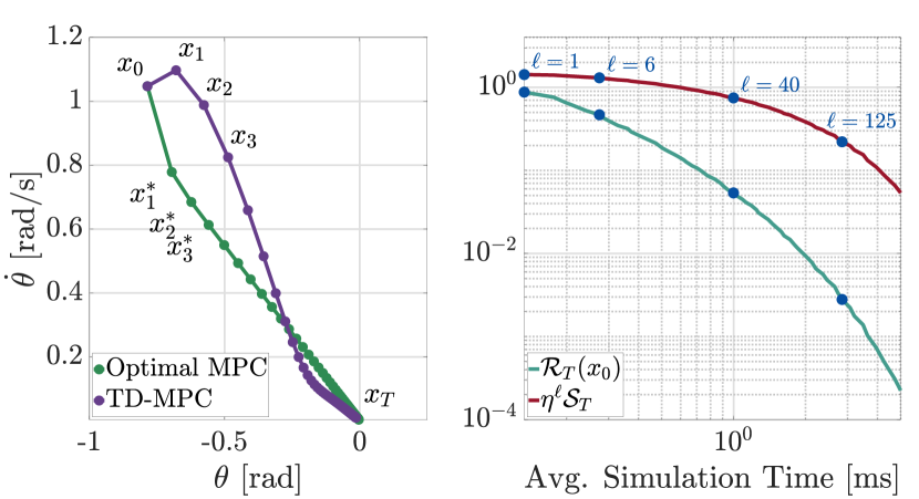
Figure 4: The phase plot on the left shows two separate trajectories generated by applying respectively TD-MPC, with a constant $\ell=6$ (in green) and optimal MPC policies (in purple). The logarithmic scale plot on the right shows the empirical suboptimality gap (in green), as well as the order of the upper bound decrease (in red) as $\ell$ and therefore the computation time are increased. The two plots on the right are parameterized by $\ell$, ranging from $1$ to $5000$.

The left panel of Figure 4 shows the evolution of two trajectories in closed-loop with the TD-MPC policy with $\ell=6$ and with an optimal MPC. For this example $\ell^{\star}=849$. However, even with the low value of $\ell=6$ the closed-loop system stays stable, as also observed in [33, 35]. Although the asymptotic/exponential stability cannot be proven, the finite time bounds can still be computed online using only the suboptimal states as per Corollary 1. The order of this upper bound, $\eta\mathcal{S}_{T}$, as well as the empirically observed suboptimality gap, $\mathcal{R}_{T}(x_{0})$, are plotted in the right panel of Figure 4 for $T=30$ for a range of values of $\ell$, increasing from $1$ to $5000$. The decrease of the suboptimality gap for increasing values of $\ell$ is juxtaposed with the increase of simulation/computational time in the same figure. The simulation time for each $\ell$ is calculated as the sum of the times it takes to solve the TD-MPC for each timestep, over the horizon $T$. To obtain an averaged value for this time, its average over $100$ repeated independent runs from the same initial conditions is taken. The initial states are intialized in $\Sigma_{N}$ following the procedure described in [35]. In the right panel of the figure, only the order of the suboptimality gap upper bound is plotted. The true constant is much larger; our aim here is not to compare the very conservative theoretical bound with the practical performance, but to give an estimate whether the bound captures the order correctly. And indeed, it can be observed from the figure that the order of the true suboptimality gap is approximately captured by the upper bound with an underestimation.

Among other possible uses of the closed-loop suboptimality analysis, the insights in the figure can be used to design the allocation of finite computational resources. The right-side plot in the figure can be used to estimate the relative gain in computational time and loss in optimality for a given change in $\ell$. For example, a change of $\ell=6$ to $\ell=31$, or equivalently $\eta^{\ell}=0.92$ to $\eta^{\ell}=0.64$ results in a $3.0$ times increase in computational time and a $1.5$ times decrease in the suboptimality gap bound, a conservative estimate of the true suboptimality gap.

6 Conclusions

We study the finite-time suboptimality gap of policies for discrete-time nonlinear, time-varying systems. We show that when the benchmark policy is chosen to be exponentially incrementally stable, then given a geometric improvement condition on the suboptimal policy, its suboptimality gap scales with its path length and improvement factor. We further show, that for non-smooth nonlinear systems E-$\delta$-ISS is implied by exponential stability under certain conditions. The assumptions are verified on the suboptimal linear quadratic MPC use case and on a numerical example. The generality of the provided analysis enables the study of other examples where the suboptimality is due to unknown system parameters or cost functions, for example in the fields of adaptive and online control. We leave the analysis of these use cases to future work.

Proof of Lemma 4

Proof.

Given a state $x\in\mathcal{D}$ and some $N\in\mathbb{R}_{+}$, let

$$V(k_{0},x)=\sum_{k=0}^{N-1}\phi(k+k_{0},k_{0},x)^{\top}\phi(k+k_{0},k_{0},x).$$

Then

$$V(k_{0},x)=x^{\top}x+\sum_{k=1}^{N-1}\phi(k+k_{0},k_{0},x)^{\top}\phi(k+k_{0},k_{0},x)\geq\|x\|^{2},$$

and, from Definition 2

$$V(k_{0},x)\leq\sum_{k=0}^{N-1}d^{2}\|x\|^{2}\lambda^{2k}\leq\frac{d^{2}}{1-\lambda^{2}}\|x\|^{2}.$$

Thus, (11) is satisfied with $c_{1}=1$ and $c_{2}=\frac{d^{2}}{1-\lambda^{2}}$. To show that (12) holds, consider

$$V(k_{0}+1,f(k_{0},x))-V(k_{0},x)$$

$$=\sum_{k=0}^{N-1}\left(\|\phi(k+k_{0}+1,k_{0},x)\|^{2}-\|\phi(k+k_{0},k_{0},x)\|^{2}\right)$$

$$=\|\phi(N+k_{0},k_{0},x)\|^{2}-\|x\|^{2}\leq d^{2}\lambda^{2N}\|x\|^{2}-\|x\|^{2}$$

$$=-\left(1-d^{2}\lambda^{2N}\right)\|x\|^{2}.$$

Choosing $N$ large enough such that $d^{2}\lambda^{2N}<1$ ensures (12) hold with $\beta^{2}=1-\frac{\left(1-d^{2}\lambda^{2N}\right)}{c_{2}}\in(0,1)$ since $c_{2}\geq c_{1}=1$ and $c_{2}\in\mathbb{R}_{+}$. Finally, for some $x,y\in\mathcal{D}$ sand $k_{0}\in\mathbb{N}$, denote $\Delta\phi(k,k_{0},x,y):=\phi(k+k_{0},k_{0},x)-\phi(k+k_{0},k_{0},y)$ and consider

$$|V(k_{0},x)-V(k_{0},y)|$$

$$=\left|\sum_{k=0}^{N-1}\left(\|\phi(k+k_{0},k_{0},x)\|^{2}-\|\phi(k+k_{0},k_{0},y)\|^{2}\right)\right|$$

$$\begin{split}&\leq\sum_{k=0}^{N-1}\left(\|\phi(k+k_{0},k_{0},x)\|+\|\phi(k+k_{0},k_{0},y)\|\right)\\ &\qquad\qquad\qquad\qquad\qquad\qquad\qquad\cdot\|\Delta\phi(k,k_{0},x,y)\|\end{split}$$

$$\leq\sum_{k=0}^{N-1}d\lambda^{k}\left(\|x\|+\|y\|\right)\cdot L_{f}^{k}\|x-y\|$$

$$=\left(\|x\|+\|y\|\right)\|x-y\|\sum_{k=0}^{N-1}d\lambda^{k}L_{f}^{k},$$

where the last inequality follows from the local exponential stability and $L_{f}$-Lipschitz continuity of the nonlinear mapping. Taking $c_{3}=\sum_{k=0}^{N-1}d\lambda^{k}L_{f}^{k}$ completes the proof. ∎

Proof of Theorem 6

The proof hinges on extending results from [29],[36], [14] and [15] . We provide all the definitions and lemmas required for the proof of Proposition 7 first.

Definition 4.

[36, 29] Given a closed, positively invariant set $\mathcal{A}\subset\mathbb{R}^{n}$, the system (9) is said to be uniformly semiglobally exponentially stable with respect to $\mathcal{A}$, if there exist constants $c,d,\in\mathbb{R}_{+}$ and $\lambda\in(0,1)$, such that

$$|\phi(k,k_{0},\xi)|_{\mathcal{A}}\leq d|\xi|_{\mathcal{A}}\lambda^{k},\qquad\forall|\xi|_{\mathcal{A}}\leq c.$$

The extension of the converse Lyapunov results from [14] and [29] to the case of semiglobal stability is included below for completeness.

Theorem 11.

If the system (9) is uniformly semiglobally exponentially stable with respect to some closed set $\mathcal{A}$ and a ROA $\mathcal{D}$, then there exists a function $V:\mathbb{N}\times\mathcal{D}\rightarrow\mathbb{R}_{+}$ and constants $c_{1},c_{2}\in\mathbb{R}_{+}$ and $\beta\in(0,1)$, such that

$$c_{1}|x|^{2}_{\mathcal{A}}\leq V(k,x)\leq c_{2}|x|^{2}_{\mathcal{A}},\qquad \forall x\in\mathcal{D},\;k\in\mathbb{N}$$ (30)

$$V\left(k+1,f(k,x)\right)\leq\beta^{2}V(k,x)\qquad \forall x\in\mathcal{D},\;k\in\mathbb{N}.$$ (31)

Proof.

Following the same line of argument from the proof of Lemma 4, consider a $x\in\mathcal{D}$ and some $N\in\mathbb{R}_{+}$ and let

$$V(k_{0},x)=\sum_{k=0}^{N-1}|\phi(k+k_{0},k_{0},x)|^{2}_{\mathcal{A}},$$ (32)

for some $k_{0}\in\mathbb{N}$. Then,

$$V(k_{0},x)=|x|^{2}_{\mathcal{A}}+\sum_{k=1}^{N-1}|\phi(k+k_{0},k_{0},x)|^{2}_{\mathcal{A}}\geq|x|^{2}_{\mathcal{A}},$$

and, from Definition 4

$$V(k_{0},x)\leq\frac{d^{2}}{1-\lambda^{2}}|x|^{2}_{\mathcal{A}}.$$

Next, consider

$$V(k_{0}+1,f(k_{0},x))-V(k_{0},x)$$

$$=\sum_{k=0}^{N-1}\left(|\phi(k_{0}+k+1,k_{0},x)|^{2}_{\mathcal{A}}-|\phi(k_{0}+k,k_{0},x)|^{2}_{\mathcal{A}}\right)$$

$$=|\phi(k_{0}+N,x)|^{2}_{\mathcal{A}}-|x|^{2}_{\mathcal{A}}\leq d^{2}\lambda^{2N}|x|^{2}_{\mathcal{A}}-|x|^{2}_{\mathcal{A}}$$

$$=-\left(1-d^{2}\lambda^{2N}\right)|x|^{2}_{\mathcal{A}}.$$

Choosing $N$ large enough such that $d^{2}\lambda^{2N}<1$ completes the proof with $c_{1}=1$, $c_{2}=\frac{d^{2}}{1-\lambda^{2}}$, and $\beta^{2}=1-\frac{\left(1-d^{2}\lambda^{2N}\right)}{c_{2}}\in(0,1)$ since $c_{2}\geq c_{1}=1$ and $c_{2}\in\mathbb{R}_{+}$. ∎

Proof of Theorem 6.

Consider the augmented system

$$\left\{\begin{array}[]{l}x_{k+1}=f(k,x_{k})\\ y_{k+1}=f(k,y_{k}).\end{array}\right.$$

The diagonal is the set $\Delta:=\{\left[x^{\top},x^{\top}\right]^{\top}\in\mathcal{D}\times\mathcal{D}:x\in\mathcal{D}\}$. Let $z:=[x^{\top},y^{\top}]^{\top}\in\mathcal{D}\times\mathcal{D}$, then it is shown in [14] that

$$|z|_{\Delta}=\frac{\sqrt{2}}{2}\|x-y\|.$$ (33)

Then, considering the evolution of the combined system

$$z_{k+1}=F(k,z_{k}):=\begin{bmatrix}f(k,x_{k})\\ f(k,y_{k})\end{bmatrix},$$ (34)

one can note that $z_{k}\in\mathcal{D}\times\mathcal{D}$ for all $k\geq k_{0},k_{0}\in\mathbb{N}$, for any $x_{k_{0}},y_{k_{0}}\in\mathcal{D}$, since $\mathcal{D}$ is forward invariant. It follows that system (9) is locally exponentially incrementally stable if and only if (34) is locally exponentially stable with respect to the diagonal $\Delta$.

Moreover, using Theorem 11, the combined system (34) admits a Lyapunov function satisfying (30)-(31). It follows from the equivalence in (33), and the proof of Theorem 11, that (15)-(16) are satisfied with $c_{1}=\frac{\sqrt{2}}{2}$, and $c_{2}=\frac{d^{2}}{\sqrt{2}-\lambda^{2}\sqrt{2}}$.

To show the inequality (17), we consider the same Lyapunov function (32) used to show (15)-(16) with $\mathcal{A}=\Delta$, i.e. given a $z\in\mathcal{D}\times\mathcal{D}$

$$V(k_{0},z)=\sum_{k=0}^{N-1}|\phi_{F}(k_{0}+k,k_{0},z)|^{2}_{\Delta},$$

where $\phi_{F}:\mathbb{N}\times\mathbb{N}\times\mathbb{R}^{2n}\rightarrow\mathbb{R}^{2n}$ is the state transition matrix for the system (34). Then, for any $x,y,\tilde{x},\tilde{y}\in\mathcal{D}$, $k\in\mathbb{N}$, $w:=[\tilde{x}^{\top},\tilde{y}^{\top}]^{\top}$ and $z$ defined as above

$$\begin{split}&|V(k_{0},z)-V(k_{0},w)|\\ &=\left|\sum_{k=0}^{N-1}\left(|\phi_{F}(k_{0}+k,k_{0},z)|^{2}_{\Delta}-|\phi_{F}(k_{0}+k,k_{0},w)|^{2}_{\Delta}\right)\right|\end{split}$$

$$\begin{split}&\leq\sum_{k=0}^{N-1}\left(\|\phi_{F}(k_{0}+k,k_{0},z)-\phi_{F}(k_{0}+k,k_{0},w)\|\right)\\ &\qquad\qquad\cdot\left(|\phi_{F}(k_{0}+k,k_{0},z)|_{\Delta}+|\phi_{F}(k_{0}+k,k_{0},w)|_{\Delta}\right)\end{split}$$

$$\begin{split}&\leq\sum_{k=0}^{N-1}\frac{d\lambda^{k}}{\sqrt{2}}\left\|\begin{bmatrix}\phi(k_{0}+k,k_{0},x)-\phi(k_{0}+k,k_{0},\tilde{x})\\ \phi(k_{0}+k,k_{0},y)-\phi(k_{0}+k,k_{0},\tilde{y})\end{bmatrix}\right\|\\ &\qquad\qquad\qquad\qquad\qquad\qquad\qquad\cdot\left(\|x-y\|+\|\tilde{x}-\tilde{y}\|\right)\end{split}$$

$$\begin{split}&\leq\left(\|x-\tilde{x}\|+\|y-\tilde{y}\|\right)\left(\|x-y\|+\|\tilde{x}-\tilde{y}\|\right)\sum_{k=0}^{N-1}\frac{d\lambda^{k}L^{k}}{\sqrt{2}},\end{split}$$

where the last two inequalities follow from the Lipschitz continuity and exponential stability (with respect to $\Delta$) of the solutions. The first inequality follows from the following. For any two vectors $x,y\in\mathcal{D}$ and closed set $\mathcal{A}$

$$|x|_{\mathcal{A}}-|y|_{\mathcal{A}} =|x|_{\mathcal{A}}-\|y-y_{p}\|\leq\|x-y_{p}\|-\|y-y_{p}\|$$

$$\leq|\|x-y_{p}\|-\|y-y_{p}\||\leq\|x-y\|,$$

where $y_{p}\in\mathcal{A}$ is such that $|y|_{\mathcal{A}}=\|y-y_{p}\|$, which exists and is unique, since $\mathcal{A}$ is closed. Finally, choosing $c_{3}=\sum_{k=0}^{N-1}\frac{d\lambda^{k}L^{k}}{\sqrt{2}}$ completes the proof. ∎

References

• [1] L. S. Pontryagin, Mathematical theory of optimal processes. CRC press, 1987.
• [2] R. Bellman, “Dynamic programming,” Science, vol. 153, no. 3731, pp. 34–37, 1966.
• [3] D. Bertsekas, Lessons from AlphaZero for optimal, model predictive, and adaptive control. Athena Scientific, 2022.
• [4] D. Bertsekas, Dynamic programming and optimal control: Volume I, vol. 4. Athena scientific, 2012.
• [5] R. S. Sutton and A. G. Barto, Reinforcement learning: An introduction. MIT press, 2018.
• [6] N. Hovakimyan and C. Cao, $\mathcal{L}1$ adaptive control theory: Guaranteed robustness with fast adaptation. SIAM, 2010.
• [7] K. S. Narendra and A. M. Annaswamy, Stable adaptive systems. Courier Corporation, 2012.
• [8] P. O. Scokaert, D. Q. Mayne, and J. B. Rawlings, “Suboptimal model predictive control (feasibility implies stability),” IEEE Transactions on Automatic Control, vol. 44, no. 3, pp. 648–654, 1999.
• [9] B. Kouvaritakis and M. Cannon, “Model predictive control,” Switzerland: Springer International Publishing, vol. 38, 2016.
• [10] Y. Li, X. Chen, and N. Li, “Online optimal control with linear dynamics and predictions: Algorithms and regret analysis,” Advances in Neural Information Processing Systems, vol. 32, 2019.
• [11] N. M. Boffi, S. Tu, and J.-J. E. Slotine, “Regret bounds for adaptive nonlinear control,” in Learning for Dynamics and Control, pp. 471–483, PMLR, 2021.
• [12] G. Belgioioso, D. Liao-McPherson, M. H. de Badyn, S. Bolognani, R. S. Smith, J. Lygeros, and F. Dörfler, “Online feedback equilibrium seeking,” arXiv preprint arXiv:2210.12088, 2022.
• [13] Z. He, S. Bolognani, J. He, F. Dörfler, and X. Guan, “Model-free nonlinear feedback optimization,” arXiv preprint arXiv:2201.02395, 2022.
• [14] D. Angeli, “A Lyapunov approach to incremental stability properties,” IEEE Transactions on Automatic Control, vol. 47, no. 3, pp. 410–421, 2002.
• [15] D. N. Tran, B. S. Rüffer, and C. M. Kellett, “Convergence properties for discrete-time nonlinear systems,” IEEE Transactions on Automatic Control, vol. 64, no. 8, pp. 3415–3422, 2018.
• [16] W. Lohmiller and J.-J. E. Slotine, “On contraction analysis for non-linear systems,” Automatica, vol. 34, no. 6, pp. 683–696, 1998.
• [17] H. Tsukamoto, S.-J. Chung, and J.-J. E. Slotine, “Contraction theory for nonlinear stability analysis and learning-based control: A tutorial overview,” Annual Reviews in Control, vol. 52, pp. 135–169, 2021.
• [18] F. Bullo, Contraction Theory for Dynamical Systems. Kindle Direct Publishing, 1.1 ed., 2023.
• [19] A. Bemporad, M. Morari, V. Dua, and E. N. Pistikopoulos, “The explicit linear quadratic regulator for constrained systems,” Automatica, vol. 38, no. 1, pp. 3–20, 2002.
• [20] A. Davydov, S. Jafarpour, and F. Bullo, “Non-euclidean contraction theory for robust nonlinear stability,” IEEE Transactions on Automatic Control, vol. 67, no. 12, pp. 6667–6681, 2022.
• [21] A. Zanelli, Q. T. Dinh, and M. Diehl, “A Lyapunov function for the combined system-optimizer dynamics in nonlinear model predictive control,” arXiv preprint arXiv:2004.08578, 2020.
• [22] D. Liao-McPherson, M. M. Nicotra, and I. Kolmanovsky, “Time-distributed optimization for real-time model predictive control: Stability, robustness, and constraint satisfaction,” Automatica, vol. 117, p. 108973, 2020.
• [23] A. Karapetyan, E. C. Balta, A. Iannelli, and J. Lygeros, “On the finite-time behavior of suboptimal linear model predictive control,” arXiv preprint arXiv:2305.10085, 2023.
• [24] B. P. Demidovich, “Lectures on stability theory (in Russian),” 1967.
• [25] A. B. Taylor, J. M. Hendrickx, and F. Glineur, “Exact worst-case convergence rates of the proximal gradient method for composite convex minimization,” Journal of Optimization Theory and Applications, vol. 178, no. 2, pp. 455–476, 2018.
• [26] H. Khalil, “Nonlinear systems, third edition, vol. 115,” Upper Saddle River, NJ, USA: Patience-Hall, 2002.
• [27] W. M. Haddad and V. Chellaboina, Nonlinear dynamical systems and control: a Lyapunov-based approach. Princeton university press, 2008.
• [28] Z.-P. Jiang, Y. Lin, and Y. Wang, “Nonlinear small-gain theorems for discrete-time feedback systems and applications,” Automatica, vol. 40, no. 12, pp. 2129–2136, 2004.
• [29] Z.-P. Jiang and Y. Wang, “A converse Lyapunov theorem for discrete-time systems with disturbances,” Systems & control letters, vol. 45, no. 1, pp. 49–58, 2002.
• [30] W. J. Rugh, Linear system theory. Prentice-Hall, Inc., 1996.
• [31] A. Pavlov, A. Pogromsky, N. van de Wouw, and H. Nijmeijer, “Convergent dynamics, a tribute to boris pavlovich demidovich,” Systems & Control Letters, vol. 52, no. 3-4, pp. 257–261, 2004.
• [32] D. Q. Mayne, J. B. Rawlings, C. V. Rao, and P. O. Scokaert, “Constrained model predictive control: Stability and optimality,” Automatica, vol. 36, no. 6, pp. 789–814, 2000.
• [33] D. Liao-McPherson, T. Skibik, J. Leung, I. Kolmanovsky, and M. M. Nicotra, “An analysis of closed-loop stability for linear model predictive control based on time-distributed optimization,” IEEE Transactions on Automatic Control, vol. 67, no. 5, pp. 2618–2625, 2021.
• [34] D. Limón, T. Alamo, F. Salas, and E. F. Camacho, “On the stability of constrained mpc without terminal constraint,” IEEE transactions on automatic control, vol. 51, no. 5, pp. 832–836, 2006.
• [35] J. Leung, D. Liao-McPherson, and I. V. Kolmanovsky, “A computable plant-optimizer region of attraction estimate for time-distributed linear model predictive control,” in 2021 American Control Conference (ACC), pp. 3384–3391, IEEE, 2021.
• [36] E. D. Sontag and Y. Wang, “New characterizations of input-to-state stability,” IEEE transactions on automatic control, vol. 41, no. 9, pp. 1283–1294, 1996.