Nonreciprocal Photon-Phonon Entanglement in Kerr-Modified Spinning Cavity Magnomechanics

Abstract

Cavity magnomechanics has shown great potential in studying macroscopic quantum effects, especially for quantum entanglement, which is a key resource for quantum information science. Here we propose to realize magnons mediated nonreciprocal photon-phonon entanglement with both the magnon Kerr and Sagnac effects in cavity magnomechanics. We find that the mean magnon number can selectively exhibit nonreciprocal linear or nonlinear (bistable) behavior with the strength of the strong driving field on the cavity. Assisted by this driving field, the magnon-phonon coupling is greatly enhanced, leading to the nonreciprocal photon-phonon entanglement via the swapping interaction between the magnons and photons. This nonreciprocal entanglement can be significantly enhanced with the magnon Kerr and Sagnac effects. Given the available parameters, the nonreciprocal photon-phonon entanglement can be preserved at $\sim 3$ K, showing remarkable resilience against the bath temperature. The result reveals that our work holds promise in developing various nonreciprocal devices with both the magnon Kerr and Sagnac effects in cavity magnomechanics.

I Introduction

Magnons Rameshti et al. (2022); Lachance-Quirion et al. (2019); Yuan et al. (2022); Prabhakar and Stancil (2009); Van Kranendonk and Van Vleck (1958), the quanta of collective spin excitations in magnetically ordered materials, especially for the yttrium iron garnet (YIG, $\rm{Y_{3}Fe_{5}O_{12}}$) Schmidt et al. (2020); Geller and Gilleo (1957); Mallmann et al. (2013), have drawn considerable attention theoretically and experimentally in quantum information science Rameshti et al. (2022); Li et al. (2020). Thanks to high spin density and low collective loss Huebl et al. (2013); Tabuchi et al. (2014); Zhang et al. (2014), magnons in YIG sphere can be strongly coupled to photons in microwave cavities for investigating various phenomena, such as dark modes Zhang et al. (2015); Bi et al. (2019), exceptional point Zhang et al. (2017, 2019a); Zhang and You (2019); Zhao et al. (2020); Cao and Yan (2019); Zhang et al. (2021a); Liu et al. (2019); Sadovnikov et al. (2022); Wang et al. (2023), nearly perfect absorption Rao et al. (2021), unconventional magnon excitations Yuan et al. (2021), , stationary one-way quantum steering Yang et al. (2021a); Guan et al. (2022), and dissipative couplings Wang et al. (2019); Wang and Hu (2020); Harder et al. (2021). With advanced experimental technologies, the magnetostrictive force, overlooked in commonly used dielectric or metallic materials, has been discovered in YIG spheres recently Zhang et al. (2016). This coupling mechanism allows magnons to interact with phonons in vibrated modes of the YIG sphere. Thus, a hybrid cavity magnomechanical (CMM) Zhang et al. (2016) system is built when a YIG sphere meets a cavity. Obviously, this hybrid system combines the individual advantages of magnons, photons and phonons, providing great potential to investigate diverse quantum effects Li et al. (2018, 2019); Hatanaka et al. (2022); Lu et al. (2021); Kani et al. (2022); Huai et al. (2019); Potts (2022). Besides, the magnon Kerr effect (i.e., the Kerr effect of magnons), caused by magnetocrystallographic anisotropy Zhang et al. (2019b); Prabhakar and Stancil (2009), was experimentally demonstrated in cavity magnonics frame Wang et al. (2018, 2016), giving rise to nonlinear cavity magnonics Zheng et al. (2023) as well as Kerr-modified CMM systems Shen et al. (2022). This nonlinearity offers a great power in studying multistability Zhang et al. (2019b); Wang et al. (2018); Shen et al. (2022); Bi et al. (2021); Yang et al. (2021b), long-distance spin-spin interaction Xiong et al. (2022, 2023); Ji and An (2023); Tian et al. (2023), quantum phase transition Liu et al. (2023); Zhang et al. (2021b), and sensitive detection Zhang et al. (2023).

In addition, macroscopic quantum entanglement has garnered significant attention in quantum information science Stannigel et al. (2012); Horodecki et al. (2009); Andersen et al. (2010); Braunstein and van Loock (2005), owing to its wide applications in quantum transduction Tian et al. (2022); Zhong et al. (2022), quantum networking  Cirac et al. (1997); Kimble (2008); Lodahl et al. (2017), quantum sensing  Degen et al. (2017), Bell-state test Marinković et al. (2018); Vivoli et al. (2016), quantum teleportation  Hofer and Hammerer (2015); Hofer et al. (2011), and microwave-optics conversion Xu et al. (2016); Tian and Li (2017); Eshaqi-Sani et al. (2022). To produce such entanglement, nonlinear effects are always required Adesso and Illuminati (2007). This results in the widespread exploration of macroscopic entanglement within nonlinear systems, including nonlinear cavity magnonics Zheng et al. (2023), CMM systems Zuo et al. (2023), and cavity optomechanics Aspelmeyer et al. (2014). Moreover, quantum entanglement can be well protected or enhanced by breaking the Lorentz reciprocity via introducing the Sagnac effect Malykin and Grigorii (2000); Maayani et al. (2018), resulting in the emergence of nonreciprocal entanglement Jiao et al. (2020). Besides the Sagnac effect, the magnon Kerr effect can also be used to achieve nonreciprocal bipartite and tripartite entanglement in cavity optomechanics Chen et al. (2023). This is due to the fact that the magnon Kerr effect can give rise to a positive or negative frequency shift on magnons as well as an additional parametric magnon amplifier under strong driving fields. However, nonreciprocal entanglement with these two nonlinear effects has yet to be revealed to date.

Here we present a scheme to realize a nonreciprocal photon-phonon entanglement in a Kerr-modified spinning CMM system, where the magnon Kerr and the Sagnac effects are both considered. The proposed system consists of the Kerr magnons in the YIG sphere simultaneously coupled to photons in the spinning cavity via the magnetic dipole interaction and phonons in the mechanical mode via magnetostrictive interaction. In this system, the mean magnon number can selectively exhibit linear or nonlinear (bistable) nonreciprocal response under the strong driving field, where the nonreciprocity is induced by the Sagnac effect, and the linear (nonlinear) behavior is caused by the interplay between the magnon Kerr effect and the magnetostrictive interaction. With the enhanced magnetostrictive coupling between the magnons and phonons by the strong driving field, magnons mediated photon-phonon entanglement can be attained via the magnon-phonon and magnon-photon swapping interaction. This achieved entanglement can be nonreciprocally improved by both the magnon Kerr and Sagnac effects with varying the tunable system parameters. Moreover, Such the nonreciprocal entanglement is robust against the bath temperature. With the available parameters, the photon-phonon entanglement can survive at $\sim 3$ K, which is much higher than previous proposals. This work provides opportunities for the development of diverse nonreciprocal devices in Kerr-modified spinning cavity magnomechanics.

This paper is organized as follows. In Sec. II, the model and the system Hamiltonian is described. Then steady-state solution and the effective Hamiltonian are given in Sec. III. In Sec. IV, the nonreciprocal photon-phonon entanglement is studied with system parameters by taking both the Sagnac and magnon Kerr effects into account. Finally, a conclusion is given in Sec. V.

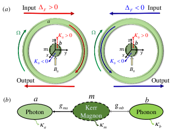
Figure 1: (a) Schematic of the Kerr-modified spinning CMM system. $K_{0}$ is the Kerr coefficient of the magnons, which can be tuned by the direction of the magnetic field $B_{0}$. When the magnetic field is aligned along the crystal axis $[100]~{}([110])$, $K_{0}>0~{}(<0)$. For the spinning cavity, a positive (negative) frequency shift $\Delta_{F}$ is produced bia the Sagnac effect when the driving field is clockwise (counterclockwise). (b) The coupling configuration. The Kerr magnons with the decay rate $\kappa_{m}$ is coupled to both the photons in the spinning cavity with the decay rate $\kappa_{a}$ and the phonons in the mechanical mode with the decay rate $\kappa_{b}$. The corresponding coupling strengths are $g_{ma}$ and $g_{mb}$.

II The model and Hamiltonian

We consider a hybrid Kerr-modified spinning cavity magnomechanical system consisting of a spinning resonator at an angular velocity $\Omega$ holding photons coupled to Kerr magnons in the Kittel mode of a $\mu$m-YIG sphere, where the magnons of the YIG sphere placed in a static magnetic field $B_{0}$ is also coupled to phonons in the mechanical mode [see Fig. 1(a)]. The Hamiltonian of the proposed hybrid system can be written as (setting $\hbar=1$)

$$H=H_{\rm SCM}+K_{0}(m^{\dagger}m)^{2}+i\epsilon_{d}(a^{\dagger}e^{-i\omega_{d}t}-ae^{i\omega_{d}t}),$$ (1)

with

$$H_{\rm SCM}= (\omega_{a}-\Delta_{F})a^{\dagger}a+\omega_{b}b^{\dagger}b+\omega_{m}m^{\dagger}m$$

$$+g_{ma}(a^{\dagger}m+am^{\dagger})+g_{mb}m^{\dagger}m(b+b^{\dagger}),$$ (2)

where $\omega_{a}$ is the resonance frequency of the non-spinning magnomechanical cavity, $\omega_{b}$ is the resonance frequency of the mechanical mode, and $\omega_{m}=\gamma H$ is the resonance frequency of the Kittel mode when the mechanical mode is at its equilibrium position, determined by the gyromagnetic ratio $\gamma$ and the external bias magnetic field $H$. $g_{ma}$ describes the coupling between the Kittel mode and the spinning cavity via the magnetic-dipole interaction, and $g_{mb}$ characterizes the single-magnon magnomechanical coupling between the Kittel mode and the mechanical mode via the magnetostrictive interaction [see Fig. 1(b)]. Experimentally, the strong magnon-photon coupling strength ($g_{ma}$) has been demonstrated Huebl et al. (2013); Tabuchi et al. (2014); Zhang et al. (2014), that is, $g_{ma}$ is larger than the dissipation rates of the cavity and Kittel modes, $\kappa_{a}$ and $\kappa_{m}$, i.e., $g_{ma}>\kappa_{a},~{}\kappa_{m}$. Typically, the magnon-phonon coupling $g_{mb}$ in the single-magnon level is weak, but it can be indirectly (directly) enhanced by imposing a strong driving field on the cavity (Kittel mode). The parameter $\Delta_{F}$ is the Sagnac-Fizeau shift of the cavity resonance frequency, induced by the light circulating in the spinning cavity, which can be given by Malykin and Grigorii (2000); Maayani et al. (2018)

$$\Delta_{F}=\pm\Omega\dfrac{nr\omega_{a}}{c}(1-\dfrac{1}{n^{2}}-\dfrac{\lambda}{n}\dfrac{dn}{d\lambda}).$$ (3)

Here, $n$ is the refractive index, $r$ is the radius of the resonator, and $\lambda$ ($c$) is the wavelength (speed) of the light in vacuum. The dispersion term $dn/d\lambda$ in Eq. (3) denotes the relativistic origin of the Sagnac effect, which is small ($\sim 1\%$) Malykin and Grigorii (2000); Maayani et al. (2018) and thus can be ignored. The sign ”$+~{}(-)$” in Eq. (3) corresponds to the clockwise (counterclockwise) driving field, where the direction of the cavity spinning is assumed to be along the clockwise direction. This means $\Delta_{F}>0$ ( $\Delta_{F}<0$ ) for the clockwise (counterclockwise) driving field [see Fig.1(a)].

The second term in Eq. (1) related to $K_{0}$ depicts the Kerr nonlinearity of the magnons in the Kittel mode of the YIG sphere, arising from the magnetocrystallographic anisotropy. The Kerr coefficient $K_{0}$ is reversely propotional to the volume of the YIG sphere Zhang et al. (2019b), and it can be tuned either positive or negative by varying the driection of the static magnetic field Wang et al. (2018). Specifically, when the magnetic field is aligned along the crystallographic axis $[100]$ ($[110]$), we have $K_{0}>0~{}(<0)$ Wang et al. (2018). Experimentally, $K_{0}$ can be tuned from $0.05$ nHz to $100$ nHz for the diameter of the YIG sphere from $1$ mm to $100$ ${\rm\mu}$m. The last term in Eq. (1) is the Hamiltonian of the driving field acting on the spinning cavity, where $\epsilon_{d}=\sqrt{2\kappa_{a}P/\omega_{d}}$ is the Rabi frequency, with $P$ being the power and $\omega_{d}$ the frequency. The operators $a~{}(a^{\dagger})$, $b~{}(b^{\dagger})$, and $m~{}(m^{\dagger})$ are the annihilation (creation) operators of the spinning cavity, the mechanical mode, and the Kittel mode, respectively. In the rotating frame respect to $\omega_{d}$, the Hamiltonian in Eq. (1) becomes

$$\mathcal{H}=\mathcal{H}_{\rm SCM}+K_{0}(m^{\dagger}m)^{2}+i\epsilon_{d}(a^{\dagger}-a),$$ (4)

where $\mathcal{H}_{\rm SCM}=H_{\rm SCM}-\omega_{d}(a^{\dagger}a+m^{\dagger}m)$.

III Quantum Langevin equation and the effective Hamiltonian

III.1 Steady state solution

By defining the frequency detuning of the spinning cavity (Kittel) mode from the driving field, i.e., $\Delta_{a(m)}=\omega_{a(m)}-\omega_{d}$, the dynamics of the considered system with dissipation can be governed by the quantum Langevin equations Walls and Milburn (1998),

$$\dot{a}= -[\kappa_{a}+i(\Delta_{a}-\Delta_{F})]a-ig_{ma}m+\epsilon_{d}+\sqrt{2\kappa_{a}}a_{\rm in},$$

$$\dot{b}= -(\kappa_{b}+i\omega_{b})b-ig_{mb}m^{\dagger}m+\sqrt{2\kappa_{b}}b_{\rm in},$$ (5)

$$\dot{m}= -(\kappa_{m}+i\Delta_{m})m-ig_{ma}a-ig_{mb}m(b+b^{\dagger})$$

$$-2iK_{0}m^{\dagger}mm+\sqrt{2\kappa_{m}}m_{\rm in}.$$

Here $\sigma_{\rm in}~{}(\sigma=a,b,m)$ are the vacuum input noise operators of the spinning cavity, the mechanical mode, and the Kittel mode, respectively. All these operators have zero mean values, i.e., $\langle\sigma_{\rm in}\rangle=0$. The correlation functions of these operators within the Markovian approximation satisfy

$$\langle\sigma_{\rm in}^{\dagger}(t^{\prime})\sigma_{\rm in}(t)\rangle= N_{\sigma}\delta(t-t^{\prime}),$$

$$\langle\sigma_{\rm in}(t)\sigma_{\rm in}^{\dagger}(t^{\prime})\rangle= (N_{\sigma}+1)\delta(t-t^{\prime}),$$ (6)

where $N_{\sigma}=[{\rm exp}({\hbar\omega_{\sigma}}/{k_{B}T}-1)]^{-1}$ is the mean thermal excitation number in the mode $\sigma$, with $k_{B}$ being the Boltzmann constant and $T$ the bath temperature.

By rewriting each operator ($\sigma$) as the sum of its expectation ($\sigma_{s}$) and fluctuation ($\sigma$) in Eq. (III.1), i.e., $\sigma\rightarrow\sigma_{s}+\sigma$, a set of equations related to the operator expectation can be given by

$$\dot{a}_{s}= -[\kappa_{a}+i(\Delta_{a}-\Delta_{F})]a_{s}-ig_{ma}m_{s}+\epsilon_{d},$$

$$\dot{b}_{s}= -(\kappa_{b}+i\omega_{b})b_{s}-ig_{mb}|m_{s}|^{2},$$ (7)

$$\dot{m}_{s}= -[\kappa_{m}+i(\tilde{\Delta}_{m}+\Delta_{K})]m_{s}-ig_{ma}a_{s},$$

where $\tilde{\Delta}_{m}=\Delta_{m}+2g_{mb}{\rm Re}[b_{s}]$ is the frequency detuning induced by the displacement of the mechanical mode ($2g_{mb}{\rm Re}[b_{s}]$), and $\Delta_{K}=2K_{0}|m_{s}|^{2}$ is the frequency shift caused by the magnon Kerr effect. In the long-time limit, the proposed system reaches its steady state, i.e., $\dot{\sigma}_{s}=0$, so Eq. (III.1) reduces to

$$[\kappa_{a}+i(\Delta_{a}-\Delta_{F})]a_{s}+ig_{ma}m_{s}-\epsilon_{d} =0,$$

$$(\kappa_{b}+i\omega_{b})b_{s}+ig_{mb}|m_{s}|^{2} =0,$$ (8)

$$[\kappa_{m}+i(\tilde{\Delta}_{m}+\Delta_{K})]m_{s}+ig_{ma}a_{s} =0.$$

By directly solving these equations, we have

$$a_{s}= \frac{\epsilon_{d}-ig_{ma}m_{s}}{\kappa_{a}+i(\Delta_{a}-\Delta_{F})},$$

$$b_{s}= -\frac{ig_{mb}|m_{s}|^{2}}{\kappa_{b}+i\omega_{b}},$$ (9)

$$m_{s}= -\frac{ig_{ma}a_{s}}{\kappa_{m}+i(\tilde{\Delta}_{m}+\Delta_{K})}.$$

Since $\Delta_{F}>0~{}(<0)$ is dependent on the direction of the clockwise (counterclockwise) driving field, so the mean photon number ($|a_{s}|^{2}$) has different values for the opposite driving fields, indicating that $|a_{s}|^{2}$ in the spinning cavity behaves nonreciprocally. This nonreciprocity can indirectly give rise to nonreciprocal mean magnon ($|m_{s}|^{2}$) and phonon ($|b_{s}|^{2}$) numbers beause of the direct coupling between the spinning cavity and the Kittel mode of the YIG sphere, and the magnon-mediated coupling between the spinning cavity and the mechanical mode [see the last two equations in Eq. (III.1)]. It is worth mentioning that such a nonreciprocal situation can also be induced by the magnon Kerr effect, even for a non-spinning cavity ($\Delta_{F}=0$). This is because $K_{0}>0$ or $K_{0}<0$, depending on the direction of the magnetic field, leads to $\Delta_{K}>0$ or $\Delta_{K}<0$. Thus, nonreciprocal mean magnon number is directly obtained [see the last equation Eq. (III.1)] and causes the nonreciprocal mean photon and phonon numbers.

III.2 Nonreciprocal bistability

From Eq. (III.1), a cubic equation related to the mean magnon number $|m_{s}|^{2}=M$ can be given by

$$[\kappa_{m}^{\prime 2}+(\Delta_{m}^{\prime}+K_{0}^{\prime}M)^{2}]M=\eta_{a}\epsilon_{d}^{2},$$ (10)

where

$$\kappa_{m}^{\prime} =\kappa_{m}+\eta_{a}\kappa_{a},$$

$$\Delta_{m}^{\prime} =\Delta_{m}-\eta_{a}(\Delta_{a}-\Delta_{F}),$$

$$K_{0}^{\prime} =2(K_{0}-\eta_{b}\omega_{b}),$$ (11)

$$\eta_{a} =\frac{g_{ma}^{2}}{\kappa_{a}^{2}+(\Delta_{a}-\Delta_{F})^{2}},$$

$$\eta_{b} =\frac{g_{mb}^{2}}{\kappa_{b}^{2}+\omega_{b}^{2}}.$$

As $K_{0}$ can be tuned via adjusting the direction of the magnetic field, so $K_{0}^{\prime}$ in Eq. (10) can be zero or nonzero. This is because that pure magnomechanical coupling [$m^{\dagger}m(b+b^{\dagger})$], similar to optomechanics, is equivalent to an effective magnon Kerr Hamiltonian by performing the unitary transformation $U=\exp[m^{\dagger}m(b-b^{\dagger})]$ Gong et al. (2008). When $K_{0}^{\prime}=0$, the cubic equation given by Eq. (10) becomes to a linear equation in the mean magnon number $M$. Obviously, it is proportional to the square of the Rabi frequency of the driving field and nonreciprocally responses to the driving fields from opposite directions, as shown in Fig. 2(a). When $K_{0}^{\prime}\neq 0$, the mean magnon number $M$ determined by Eq. (10) can have two switching points for bistability under the specific parameter conditions [see Fig. 2(b)], at which there must be $d\epsilon_{d}/dM=0$, i.e.,

$$3K_{0}^{\prime 2}M^{2}+4K_{0}^{\prime}\Delta_{m}^{\prime}M+\kappa_{m}^{\prime 2}+\Delta_{m}^{\prime 2}=0.$$ (12)

This equation has two real roots, corresponding to two switching points of the bistability, only when the root discriminant satisfies the inequality $\Delta_{m}^{\prime 2}-3\kappa_{m}^{\prime 2}>0$, i.e.,

$$\Delta_{m}^{\prime}>\sqrt{3}\kappa_{m}^{\prime}~{}{\rm or}~{}\Delta_{m}^{\prime}<-\sqrt{3}\kappa_{m}^{\prime}.$$ (13)

In particular, when $\Delta_{m}^{\prime 2}-3\kappa_{m}^{\prime 2}=0$, i.e., $\Delta_{m}^{\prime}=\pm\sqrt{3}\kappa_{m}^{\prime}$, Eq. (12) has two equal real roots ($M_{1(2)}=-2\Delta_{m}^{\prime}/3K_{0}^{\prime}$), that is, two switching points coalesce to one point, indicating no bistability. This give rise to a critical driving strength,

$$\epsilon_{d}^{c}=\sqrt{-8\kappa_{m}^{\prime 2}\Delta_{m}^{\prime}/9\eta_{a}K_{0}^{\prime}}=\sqrt{\pm 8\kappa_{m}^{\prime 3}/9\eta_{a}K_{0}^{\prime}},$$ (14)

where the positive (negative) simbol denotes $K_{0}^{\prime}>0$ and $\Delta_{m}^{\prime}<0$ ($K_{0}^{\prime}<0$ and $\Delta_{m}^{\prime}>0$). Eq. (14) indicates that magnonic bistability can be predicted when the strength of the driving field exceeds the critical value, i.e., $\epsilon_{d}>\epsilon_{d}^{c}$, as shown in Fig. 2(b). Due to different responses of the spinning cavity to the CW or CCW driving field, nonreciprocal bistability can be apparently observed [see the red and blue curves in Fig. 2(b)].

III.3 Fluctuation dynamics

Apart from the steady state dynamics when the transformation $\sigma\rightarrow\sigma_{s}+\sigma$ is substituted into Eq. (III.1), the fluctation dynamics can also be obtained,

$$\dot{a}= -[\kappa_{a}+i(\Delta_{a}-\Delta_{F})]a-ig_{ma}m+\sqrt{2\kappa_{a}}a_{\rm in},$$

$$\dot{b}= -(\kappa_{b}+i\omega_{b})b-i(G_{mb}m^{\dagger}+G_{mb}^{*}m)+g_{mb}m^{\dagger}m$$

$$+\sqrt{2\kappa_{b}}b_{\rm in},$$ (15)

$$\dot{m}= -[\kappa_{m}+i(\tilde{\Delta}_{m}+2\Delta_{K})]m-ig_{ma}a+\sqrt{2\kappa_{m}}m_{\rm in}$$

$$-ig_{mb}m(b+b^{\dagger})-2iK_{0}m_{s}^{2}m^{\dagger}-iG_{mb}(b+b^{\dagger})$$

$$-2iK_{0}(m_{s}^{*}m^{2}+2m_{s}m^{\dagger}m+m^{\dagger}m^{2}),$$

where $G_{mb}=g_{mb}m_{s}$ is the effective magnomechanical coupling strength significantly enhanced by multiple magnons. Below we assume that $m_{s}$ is real for simplicity. This can be realized by choosing the propoer phase of the driving field according to Eq. (III.1). Under the strong driving field (i.e., $|m_{s}|\gg 1$), Eq. (III.3) can be linearized by safely ignoring the high-order fluctuations. As a result, Eq. (III.3) reduces to

$$\dot{a}= -[\kappa_{a}+i(\Delta_{a}-\Delta_{F})]a-ig_{ma}m+\sqrt{2\kappa_{a}}a_{\rm in},$$

$$\dot{b}= -(\kappa_{b}+i\omega_{b})b-iG_{mb}(m^{\dagger}+m)+\sqrt{2\kappa_{b}}b_{\rm in},$$

$$\dot{m}= -[\kappa_{m}+i(\tilde{\Delta}_{m}+2\Delta_{K})]m-i\Delta_{K}m^{\dagger}-ig_{ma}a$$

$$-iG_{mb}(b+b^{\dagger})+\sqrt{2\kappa_{m}}m_{\rm in}.$$ (16)

We then rewrite the above equations as $\dot{\sigma}=i[H_{\rm eff},\sigma]-\kappa_{\sigma}\sigma+\sqrt{2\kappa_{\sigma}}\sigma_{\rm in}$, so the effective Hamiltonian of the linearized system can be given by

$$H_{\rm eff}= (\Delta_{a}-\Delta_{F})a^{\dagger}a+\omega_{b}b^{\dagger}b+(\tilde{\Delta}_{m}+2\Delta_{K})m^{\dagger}m$$

$$+g_{ma}(a^{\dagger}m+am^{\dagger})+\frac{\Delta_{K}}{2}(m^{\dagger}m^{\dagger}+mm)$$

$$+G_{mb}(m^{\dagger}+m)(b^{\dagger}+b).$$ (17)

Note that the two-magnon effect (i.e., $m^{\dagger}m^{\dagger}+mm$) stems from the magnon Kerr nonlinearity in the presence of the strong driving field, which can be well tuned by varying the Rabi frequency of the driving field.

IV The nonreciprocal photon-phonon entanglement

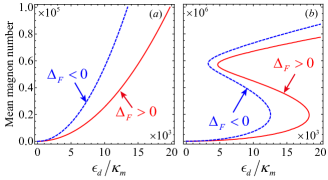
Figure 2: The mean magnon number versus the normalized amplitude of the driving field with (a) $K_{0}=\eta_{b}\omega_{b}$ and (b) $K_{0}=0.1\eta_{b}\omega_{b}$, where $\omega_{b}/2\pi=10$ MHz, $\kappa_{a}=\kappa_{m}=0.1\omega_{b}$, $\kappa_{b}/2\pi=100$ Hz, $g_{\rm ma}=0.2\omega_{b}$, $g_{mb}=10^{-3}\omega_{b}$, $|\Delta_{F}|=0.2\omega_{b}$, $\Delta_{a}=-\omega_{b}$, and $\Delta_{m}=\omega_{b}$.

With the effective Hamiltonian $H_{\rm eff}$ in hand, its dynamics governed by Eq. (III.3) can be rewritten in a more compact form as $\dot{u}(t)=Au(t)+f(t)$, where $u^{T}(t)=(X_{a},Y_{a},X_{m},Y_{m},X_{b},Y_{b})$ is the vector operator of the system, $f^{T}(t)=(\sqrt{2\kappa_{a}}X_{a}^{\rm in}$, $\sqrt{2\kappa_{a}}Y_{a}^{\rm in}$, $\sqrt{2\kappa_{m}}X^{\rm in}_{m}$, $\sqrt{2\kappa_{m}}Y^{\rm in}_{m}$, $\sqrt{2\kappa_{b}}X^{\rm in}_{b}$, $\sqrt{2\kappa_{b}}Y^{\rm in}_{b})$ is the input noise of the system, and

$$\small{A=\left(\begin{array}[]{cccccc}-\kappa_{a}&{\Delta}_{a}-\Delta_{F}&0&g_{ma}&0&0\\ -{\Delta}_{a}+\Delta_{F}&-\kappa_{a}&-g_{\rm ma}&0&0&0\\ 0&g_{ma}&-\kappa_{m}&\tilde{\Delta}_{m}+\Delta_{K}&0&0\\ -g_{ma}&0&-\widetilde{\Delta}_{m}-3\Delta_{K}&-\kappa_{m}&-2G_{mb}&0\\ 0&0&0&0&-\kappa_{b}&\omega_{b}\\ 0&0&-2G_{mb}&0&-\omega_{b}&-\kappa_{b}\end{array}\right)}$$ (18)

is the drift matrix. Here $X_{\sigma}=(\sigma^{\dagger}+\sigma)/\sqrt{2}$, $Y_{\sigma}=i(\sigma^{\dagger}-\sigma)/\sqrt{2}$, $X_{\sigma}^{\rm in}=(\sigma_{\rm in}^{\dagger}+\sigma_{\rm in})/\sqrt{2}$, and $Y_{\sigma}^{\rm in}=i(\sigma_{\rm in}^{\dagger}-\sigma_{\rm in})/\sqrt{2}$.

Since the input quantum noises are zero-mean quantum Gaussian noises, the quantum steady state for the fluctuations is a zero-mean continuous variable Gaussian state, fully characterized by a $6\times 6$ correlation matrix $V_{ij}^{(6)}=\langle u_{i}(\infty)u_{j}(\infty)+u_{j}(\infty)u_{i}(\infty)\rangle$ ($i,j=1,2,\ldots,6$). The matrix $V$ can be obtained by directly solving the Lyapunov equation,

$$AV+VA^{\dagger}=-D,$$ (19)

where the diffusion matrix $D={\rm diag}[\kappa_{a}(2N_{a}+1),\kappa_{a}(2N_{a}+1),\kappa_{m}(2N_{m}+1),\kappa_{m}(2N_{m}+1),\kappa_{b}(2N_{b}+1),\kappa_{b}(2N_{b}+1)]$ is defined by $D_{ij}\delta(t-t^{\prime})=\langle v_{i}(t)v_{j}(t^{\prime})+v_{j}(t^{\prime})v_{i}(t)\rangle/2$. Once the matrix $V$ is obtained, one can investigate arbitrary bipartite entanglement of interest in the proposed system via the logarithmic negativity

$$E_{N}\equiv\rm max[0,-ln2\eta^{-}],$$ (20)

with

$$\eta^{-}=2^{-1/2}[\Sigma-(\Sigma^{2}-4\rm det{V}_{4})^{1/2}]^{1/2},$$ (21)

where $\Sigma=\rm{det}\mathcal{A}+\rm{det}\mathcal{B}-2\rm{det}\mathcal{C}$ and ${V}_{4}=\begin{pmatrix}\mathcal{A}&\mathcal{C}\\ \mathcal{C^{T}}&\mathcal{B}\\ \end{pmatrix}$ is the $4\times 4$ block form of the correlation matrix, associated with two modes of interest. $\mathcal{A}$, $\mathcal{B}$, and $\mathcal{C}$ are the $2\times 2$ blocks of $V_{4}$. A positive logarithmic negativity ($E_{N}>0$) denotes the presence of bipartite entanglement of the interested two modes in the considered system.

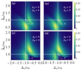
Figure 3: Density plot of the photon-phonon entanglement $E_{ab}$ as functions of $\Delta_{a}/\omega_{b}$ and $\tilde{\Delta}_{m}/\omega_{b}$ with (a) $\Delta_{K}>0$, $\Delta_{F}>0$, (b) $\Delta_{K}>0$, $\Delta_{F}<0$, (c) $\Delta_{K}<0$, $\Delta_{F}>0$, and (d) $\Delta_{K}<0$, $\Delta_{F}<0$. Other parameters are the same as those in Fig. 2 except for $G_{mb}=g_{ma}$, $|\Delta_{K}|=0.2\omega_{b}$, and the bath temperature $T=10$ mK.

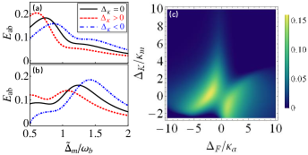
Figure 4: The photon-phonon entanglement versus $\tilde{\Delta}_{m}/\omega_{b}$ with and without the magnon Kerr effect in the left panel (a, b) and $\Delta_{K}$ and $\Delta_{F}$ in the right panel (c), where (a) $\Delta_{F}>0$ and (b) $\Delta_{F}<0$. Other parameters in (a-c) are the same as those in Fig. 2.

We first plot the logarithmic negativity $E_{ab}$ as functions of the normalized $\Delta_{a}/\omega_{b}$ and $\tilde{\Delta}_{m}/\omega_{b}$ in the presence of both the Sagnac and the magnon Kerr effects in Fig. 3, where $G_{\rm mb}/2\pi=|\Delta_{k}|=0.2\omega_{b}$, the bath temperature $T=10$ mK, and other parameters are the same as those in Fig. 2. The chosen parameters ensure the system stable following the Routh-Hurwitz criterion. From Fig. 3, one can see that the photon-phonon entanglement can be tuned by changing the frequency detunings $\Delta_{a}$ and $\tilde{\Delta}_{m}$. In particular, its optimal value is predicted at $\Delta_{a}\approx-\omega_{b}+\Delta_{F}$ and $\tilde{\Delta}_{m}\approx\omega_{b}-2\Delta_{K}$. The mechanism of this optimal entanglement can be interpreted as follows: When $\tilde{\Delta}_{m}\approx\omega_{b}-2\Delta_{K}$, the magnomechanical subsystem is driven to the red sideband, where the mechanical mode can be well cooled for allowing considerable magnon-phonon entanglement owing to the enhanced magnomechanical coupling $G_{mb}$. Then the magnon-phonon entanglement is significantly transferred to the photon-phonon entanglement via the beam splitter magnon-photon interaction at $\Delta_{a}\approx-\omega_{b}+\Delta_{F}$. From Fig. 3, we find that the predicted photon-phonon entanglement nonreciprocally response to the change of the frequency detunings $\Delta_{K}$ or $\Delta_{F}$, i.e., the magnon Kerr or the Sagnac effect. This means that the nonreciprocal photon-photon entanglement can be achieved by including these two effects. Specifically, when $\Delta_{F}>0$, the optimal cavity frequency detuning is fixed at $\Delta_{a}\approx-0.8\omega_{b}$, but the optimal magnon frequency detuning is $\tilde{\Delta}_{m}\approx 0.6\omega_{b}$ for $\Delta_{K}>0$ [Fig. 3(a)] and $\tilde{\Delta}_{m}\approx 1.4\omega_{b}$ for $\Delta_{K}<0$ [Fig. 3(c)]. This indicates that the photon-phonon entanglement nonreciprocally responses to the opposite magnetic fields when the magnon Kerr effect is considered with the fixed Sagnac effect. The similar result can also be obtained from Figs. 3(b) and 3(d). By comparing Figs. 3(a) with 3(b) [or Figs. 3(c) with 3(d)], we show that the optimal photon-phonon entanglement is predicted at different cavity frequency detunnings $\Delta_{a}$ but at the same magnon frequency detuning $\tilde{\Delta}_{m}$. This means the nonreciprocal photon-phonon entanglement can also be induced by the Sagnac effect for the fixed magnetic field in the presence of the magnon Kerr effect. Figures 4(a) and 4(b) futher show the nonreciprocal behavior of the photon-phonon entanglement with the normalized $\tilde{\Delta}_{m}/\omega_{b}$ in the presence of the magnon and Sagnac effects, where $\Delta_{a}=-\omega_{b}$. For $\Delta_{F}>0$ [see Fig. 4(a)], we find that the photon-phonon entanglement can be nonreciprocally enhanced ($\Delta_{K}>0$) or reduced ($\Delta_{K}>0$), compared to the case without the magnon Kerr effect. In the case of $\Delta_{F}<0$ [see Fig. 4(b)], the situation becomes opposite. From Fig. 4(a) and 4(b), one can see that the photon-phonon entanglement can also be nonreciprocally enhanced or reduced by the Sagnac effect for the fixed magnon Kerr effect. Figure 4(c) directly reveals the behavior of the photon-phonon entanglement with these two effects. Obviously, the nonreciprocal photon-phonon entanglement can be achieved by using the magnon Kerr effect or the Sagnac effect or both of them. The optimal value of the photon-phonon entanglement can be approximately predicted at $\Delta_{K}\Delta_{F}<0$.

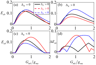
Figure 5: The photon-phonon entanglement versus $G_{mb}/g_{ma}$ with (a) $\Delta_{K}=0$, (b) $\Delta_{K}>0$, (c) $\Delta_{K}<0$, wehre the Sagnac effect are all considered. (d) The nonreciprocity of the photon-phonon entanglement induced by the magnon Kerr effect versus $G_{mb}/g_{ma}$ with and without the Sagnac effect. Other parameters in (a-c) are the same as those in Fig. 2.

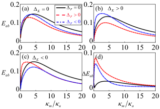
Figure 6: The photon-phonon entanglement versus $\kappa_{m}/\kappa_{a}$ with (a) $\Delta_{K}=0$, (b) $\Delta_{K}>0$, (c) $\Delta_{K}<0$, wehre the Sagnac effect are all considered. (d) The nonreciprocity of the photon-phonon entanglement induced by the magnon Kerr effect versus $\kappa_{m}/\kappa_{a}$ with and without the Sagnac effect. Other parameters in (a-c) are the same as those in Fig. 2.

In fact, the magnomechanical coupling strength $G_{mb}$ can be fine-tuned by adjusting the Rabi frequency of the driving field on the cavity [see Eq. (III.1)] in our proposal. So how does the magnomechanical coupling affect the photon-phonon entanglement with or without the magnon Kerr and Sagnac effects? To show this, we plot $E_{ab}$ versus the normalized coupling strength $G_{mb}/g_{ma}$ in Figs. 5(a-c). Obviously, the photon-phonon entanglement increases first to its maximal value and then decreases with the magnomechanical coupling strength $G_{mb}/g_{ma}$. Specifically, the Sagnac effect can only give a weak nonreciprocity on the photon-phonon entanglement in the absence of the magnon Kerr effect $\Delta_{K}=0$ [see Fig. 5(a)]. In the presence of the magnon Kerr effect ($\Delta_{K}\neq 0$), we find that a visible nonreciprocity on the photon-phonon entanglement can be induced by the Sagnac effect [see Fig. 5(b) or 5(c)]. This is because that the photon-phonon entanglement can be significantly enhanced (reduced) when $\Delta_{K}\Delta_{F}<0$ ($\Delta_{K}\Delta_{F}>0$). From Figs. 5(a-c), the magnon Kerr effect induced nonreciprocity on the photon-phonon entanglement can also be revealed with or without the Sagnac effect. More intuitively, we plot the difference ($\Delta E_{ab}$) of the logarithmic negativities between the cases of $\Delta_{K}>0$ and $\Delta_{K}<0$ in Fig. 5(d), where $\Delta E_{ab}$ is defined as

$$\Delta E_{ab}=|E_{ab}(\Delta_{K}>0)-E_{ab}(\Delta_{K}<0)|.$$ (22)

When the Sagnac effect is included, we find that large $\Delta E_{ab}$ can be obtained, as shown by the red and blue curves.

Besides the magnomechanical coupling strength, the decay rate of the magnons in the Kittel mode of the YIG sphere can also be adjusted experimentally via changing the distance between the YIG sphere and the microwave attenna. We find that the optimal photon-phonon entanglement can be realized by tuning $\kappa_{m}$ when other paraters are fixed, as shown in Figs. 6(a-c). In the absence of the magnon Kerr effect, i.e., $\Delta_{K}=0$, one can see that the photon-phonon entanglement is rubust against the Sagnac effect for the small decay rate of the Kittel mode [see Fig. 6(a)], but when the magnon Kerr effect is taken into account, i.e., $\Delta_{K}\neq 0$, the visible nonreciprocity induced by the Sagnac effect can be predicted [see Fig. 6(b) or 6(c)]. We also show that the nonreciprocity induced by the Sagnac effect in the presence or absence of the magnon Kerr effect can be suppressed by increasing $\kappa_{m}$. This means that the nonreciprocity induced by the Sagnac effect can only be observed for the proper value of $\kappa_{m}$. The similar result can also be obtained for the magnon Kerr effect induced nonreciprocity of the photon-phonon entanglement with or without the Sagnac effect [see Fig. 6(d)].

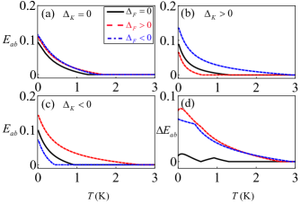
Figure 7: The photon-phonon entanglement versus the bath temperature $T$ with (a) $\Delta_{K}=0$, (b) $\Delta_{K}>0$, (c) $\Delta_{K}<0$, wehre the Sagnac effect are all considered. (d) The nonreciprocity of the photon-phonon entanglement induced by the magnon Kerr effect versus $T$ with and without the Sagnac effect. Other parameters in (a-c) are the same as those in Fig. 2.

Next, we check the effect of the bath temperature on the photon-phonon entanglement in our proposal. For this, we plot the logarithmic negativity $E_{ab}$ versus the temperature $T$ with or without the magnon Kerr and the Sagnac effects in Fig. 7(a-c). Figure 7(a) shows that the Sagnac effect can only cause a slight enhancement on the photon-phonon entanglement at $\Delta_{K}=0$. When the magnon Kerr effect is included, we find that both the photon-phonon entanglement and its survival temperature are nonreciprocally improved (reduced) by the Sagnac effect at $\Delta_{K}\Delta_{F}<0~{}(\Delta_{K}\Delta_{F}>0)$ [see Figs. 7(b) and 7(c)]. Notably, the survival temperature of the photon-phonon entanglement in our proposal can be improved to $\sim 3$ K, which is about $15$ times than the previous proposal Li et al. (2018). Figure  7(d) also demonstrates that the magnon Kerr effect has the same effect on photon-phonon entanglement as the Sagnac effect.

V CONCLUSION

In summary, we have proposed a proposal to generate a nonreciprocal photon-phonon entanglement in a Kerr-modified spinning cavity magnomechanics. The mean magnon number here can selectively display nonreciprocal linear or nonlinear (bistable) behavior with the strength of the strong driving field, where the nonreciprocity arises from the Sagnac effect, and the linear (nonlinear) behavior is the result of the interplay between the magnon Kerr effect and the magnetostrictive effect. With the enhanced magnon-phonon coupling and the swapping interaction between the magnons and the photons, magnons mediated photon-phonon entanglement is generated. This entanglement can be nonreciprocally enhanced with taking both the Sagnac and the magnon Kerr effects into account. We also show that the achieved nonreciprocal entanglement can be kept up to $\sim 3$ K with accessible parameters, exhibiting great potential in robust against the bath temperature. Our work provides a promising way to engineer various nonreciprocal devices with the magnon Kerr and the Sagnac effects in cavity magnomechanics.

References

- Rameshti et al. (2022) B. Z. Rameshti, S. V. Kusminskiy, J. A. Haigh, K. Usami, D. Lachance-Quirion, Y. Nakamura, C.-M. Hu, H. X. Tang, G. E. Bauer, and Y. M. Blanter, Physics Reports 979, 1 (2022).
- Lachance-Quirion et al. (2019) D. Lachance-Quirion, Y. Tabuchi, A. Gloppe, K. Usami, and Y. Nakamura, Applied Physics Express 12, 070101 (2019).
- Yuan et al. (2022) H. Yuan, Y. Cao, A. Kamra, R. A. Duine, and P. Yan, Physics Reports 965, 1 (2022).
- Prabhakar and Stancil (2009) A. Prabhakar and D. D. Stancil, Spin waves: Theory and applications, vol. 5 (Springer, 2009).
- Van Kranendonk and Van Vleck (1958) J. Van Kranendonk and J. Van Vleck, Reviews of Modern Physics 30, 1 (1958).
- Schmidt et al. (2020) G. Schmidt, C. Hauser, P. Trempler, M. Paleschke, and E. T. Papaioannou, physica status solidi (b) 257, 1900644 (2020).
- Geller and Gilleo (1957) S. Geller and M. Gilleo, Journal of Physics and Chemistry of solids 3, 30 (1957).
- Mallmann et al. (2013) E. Mallmann, A. Sombra, J. Goes, and P. Fechine, Solid State Phenomena 202, 65 (2013).
- Li et al. (2020) Y. Li, W. Zhang, V. Tyberkevych, W.-K. Kwok, A. Hoffmann, and V. Novosad, Journal of Applied Physics 128 (2020).
- Huebl et al. (2013) H. Huebl, C. W. Zollitsch, J. Lotze, F. Hocke, M. Greifenstein, A. Marx, R. Gross, and S. T. Goennenwein, Physical Review Letters 111, 127003 (2013).
- Tabuchi et al. (2014) Y. Tabuchi, S. Ishino, T. Ishikawa, R. Yamazaki, K. Usami, and Y. Nakamura, Physical Review Letters 113, 083603 (2014).
- Zhang et al. (2014) X. Zhang, C.-L. Zou, L. Jiang, and H. X. Tang, Physical Review Letters 113, 156401 (2014).
- Zhang et al. (2015) X. Zhang, C.-L. Zou, N. Zhu, F. Marquardt, L. Jiang, and H. X. Tang, Nature communications 6, 8914 (2015).
- Bi et al. (2019) M. Bi, X. Yan, Y. Xiao, and C. Dai, Journal of Applied Physics 126 (2019).
- Zhang et al. (2017) D. Zhang, X.-Q. Luo, Y.-P. Wang, T.-F. Li, and J. You, Nature communications 8, 1368 (2017).
- Zhang et al. (2019a) X. Zhang, K. Ding, X. Zhou, J. Xu, and D. Jin, Physical Review Letters 123, 237202 (2019a).
- Zhang and You (2019) G.-Q. Zhang and J. You, Physical Review B 99, 054404 (2019).
- Zhao et al. (2020) J. Zhao, Y. Liu, L. Wu, C.-K. Duan, Y.-x. Liu, and J. Du, Physical Review Applied 13, 014053 (2020).
- Cao and Yan (2019) Y. Cao and P. Yan, Physical Review B 99, 214415 (2019).
- Zhang et al. (2021a) G.-Q. Zhang, Z. Chen, D. Xu, N. Shammah, M. Liao, T.-F. Li, L. Tong, S.-Y. Zhu, F. Nori, and J. You, PRX Quantum 2, 020307 (2021a).
- Liu et al. (2019) H. Liu, D. Sun, C. Zhang, M. Groesbeck, R. Mclaughlin, and Z. V. Vardeny, Science advances 5, eaax9144 (2019).
- Sadovnikov et al. (2022) A. V. Sadovnikov, A. A. Zyablovsky, A. V. Dorofeenko, and S. A. Nikitov, Physical Review Applied 18, 024073 (2022).
- Wang et al. (2023) X.-g. Wang, L.-l. Zeng, G.-h. Guo, and J. Berakdar, Physical Review Letters 131, 186705 (2023).
- Rao et al. (2021) J. Rao, P. Xu, Y. Gui, Y. Wang, Y. Yang, B. Yao, J. Dietrich, G. Bridges, X. Fan, D. Xue, et al., Nature communications 12, 1933 (2021).
- Yuan et al. (2021) H. Yuan, S. Zheng, Q. He, J. Xiao, and R. A. Duine, Physical Review B 103, 134409 (2021).
- Yang et al. (2021a) Z.-B. Yang, X.-D. Liu, X.-Y. Yin, Y. Ming, H.-Y. Liu, and R.-C. Yang, Physical Review Applied 15, 024042 (2021a).
- Guan et al. (2022) S.-Y. Guan, H.-F. Wang, and X. Yi, npj Quantum Information 8, 102 (2022).
- Wang et al. (2019) Y.-P. Wang, J. Rao, Y. Yang, P.-C. Xu, Y. Gui, B. Yao, J. You, and C.-M. Hu, Physical Review Letters 123, 127202 (2019).
- Wang and Hu (2020) Y.-P. Wang and C.-M. Hu, Journal of Applied Physics 127 (2020).
- Harder et al. (2021) M. Harder, B. Yao, Y. Gui, and C.-M. Hu, Journal of Applied Physics 129 (2021).
- Zhang et al. (2016) X. Zhang, C.-L. Zou, L. Jiang, and H. X. Tang, Science advances 2, e1501286 (2016).
- Li et al. (2018) J. Li, S.-Y. Zhu, and G. Agarwal, Physical Review Letters 121, 203601 (2018).
- Li et al. (2019) J. Li, S.-Y. Zhu, and G. Agarwal, Physical Review A 99, 021801 (2019).
- Hatanaka et al. (2022) D. Hatanaka, M. Asano, H. Okamoto, Y. Kunihashi, H. Sanada, and H. Yamaguchi, Physical Review Applied 17, 034024 (2022).
- Lu et al. (2021) T.-X. Lu, H. Zhang, Q. Zhang, and H. Jing, Physical Review A 103, 063708 (2021).
- Kani et al. (2022) A. Kani, B. Sarma, and J. Twamley, Physical Review Letters 128, 013602 (2022).
- Huai et al. (2019) S.-N. Huai, Y.-L. Liu, J. Zhang, L. Yang, and Y.-x. Liu, Physical Review A 99, 043803 (2019).
- Potts (2022) C. Potts (2022).
- Zhang et al. (2019b) G. Zhang, Y. Wang, and J. You, Science China Physics, Mechanics & Astronomy 62, 1 (2019b).
- Wang et al. (2018) Y.-P. Wang, G.-Q. Zhang, D. Zhang, T.-F. Li, C.-M. Hu, and J. You, Physical Review Letters 120, 057202 (2018).
- Wang et al. (2016) Y.-P. Wang, G.-Q. Zhang, D. Zhang, X.-Q. Luo, W. Xiong, S.-P. Wang, T.-F. Li, C.-M. Hu, and J. You, Physical Review B 94, 224410 (2016).
- Zheng et al. (2023) S. Zheng, Z. Wang, Y. Wang, F. Sun, Q. He, P. Yan, and H. Yuan, arXiv preprint arXiv:2303.16313 (2023).
- Shen et al. (2022) R.-C. Shen, J. Li, Z.-Y. Fan, Y.-P. Wang, and J. You, Physical Review Letters 129, 123601 (2022).
- Bi et al. (2021) M. Bi, X. Yan, Y. Zhang, and Y. Xiao, Physical Review B 103, 104411 (2021).
- Yang et al. (2021b) Z.-B. Yang, H. Jin, J.-W. Jin, J.-Y. Liu, H.-Y. Liu, and R.-C. Yang, Physical Review Research 3, 023126 (2021b).
- Xiong et al. (2022) W. Xiong, M. Tian, G.-Q. Zhang, and J. You, Physical Review B 105, 245310 (2022).
- Xiong et al. (2023) W. Xiong, M. Wang, G.-Q. Zhang, and J. Chen, Physical Review A 107, 033516 (2023).
- Ji and An (2023) F.-Z. Ji and J.-H. An, arXiv preprint arXiv:2308.05927 (2023).
- Tian et al. (2023) M. Tian, M. Wang, G.-Q. Zhang, H.-C. Li, and W. Xiong, arXiv preprint arXiv: 2304.13553 (2023).
- Liu et al. (2023) G. Liu, W. Xiong, and Z.-J. Ying, arXiv preprint arXiv:2302.07163 (2023).
- Zhang et al. (2021b) G.-Q. Zhang, Z. Chen, W. Xiong, C.-H. Lam, and J. You, Physical Review B 104, 064423 (2021b).
- Zhang et al. (2023) G.-Q. Zhang, Y. Wang, and W. Xiong, Physical Review B 107, 064417 (2023).
- Stannigel et al. (2012) K. Stannigel, P. Komar, S. J. M. Habraken, S. D. Bennett, M. D. Lukin, P. Zoller, and P. Rabl, Phys. Rev. Lett. 109, 013603 (2012).
- Horodecki et al. (2009) R. Horodecki, P. Horodecki, M. Horodecki, and K. Horodecki, Rev. Mod. Phys. 81, 865 (2009).
- Andersen et al. (2010) U. Andersen, G. Leuchs, and C. Silberhorn, Laser & Photonics Reviews 4, 337 (2010).
- Braunstein and van Loock (2005) S. L. Braunstein and P. van Loock, Rev. Mod. Phys. 77, 513 (2005).
- Tian et al. (2022) T. Tian, Y. Zhang, L. Zhang, L. Wu, S. Lin, J. Zhou, C.-K. Duan, J.-H. Jiang, and J. Du, Physical Review Letters 129, 215901 (2022).
- Zhong et al. (2022) C. Zhong, X. Han, and L. Jiang, Physical Review Applied 18, 054061 (2022).
- Cirac et al. (1997) J. I. Cirac, P. Zoller, H. J. Kimble, and H. Mabuchi, Physical Review Letters 78, 3221 (1997).
- Kimble (2008) H. J. Kimble, Nature 453, 1023 (2008).
- Lodahl et al. (2017) P. Lodahl, S. Mahmoodian, S. Stobbe, A. Rauschenbeutel, P. Schneeweiss, J. Volz, H. Pichler, and P. Zoller, Nature 541, 473 (2017).
- Degen et al. (2017) C. L. Degen, F. Reinhard, and P. Cappellaro, Reviews of modern physics 89, 035002 (2017).
- Marinković et al. (2018) I. Marinković, A. Wallucks, R. Riedinger, S. Hong, M. Aspelmeyer, and S. Gröblacher, Physical Review Letters 121, 220404 (2018).
- Vivoli et al. (2016) V. C. Vivoli, T. Barnea, C. Galland, and N. Sangouard, Physical Review Letters 116, 070405 (2016).
- Hofer and Hammerer (2015) S. G. Hofer and K. Hammerer, Physical Review A 91, 033822 (2015).
- Hofer et al. (2011) S. G. Hofer, W. Wieczorek, M. Aspelmeyer, and K. Hammerer, Physical Review A 84, 052327 (2011).
- Xu et al. (2016) X.-W. Xu, Y. Li, A.-X. Chen, and Y.-x. Liu, Phys. Rev. A 93, 023827 (2016).
- Tian and Li (2017) L. Tian and Z. Li, Phys. Rev. A 96, 013808 (2017).
- Eshaqi-Sani et al. (2022) N. Eshaqi-Sani, S. Zippilli, and D. Vitali, Phys. Rev. A 106, 032606 (2022).
- Adesso and Illuminati (2007) G. Adesso and F. Illuminati, Journal of Physics A: Mathematical and Theoretical 40, 7821 (2007).
- Zuo et al. (2023) X. Zuo, Z.-Y. Fan, H. Qian, M.-S. Ding, H. Tan, H. Xiong, and J. Li, arXiv preprint arXiv: 2310.19237 (2023).
- Aspelmeyer et al. (2014) M. Aspelmeyer, T. J. Kippenberg, and F. Marquardt, Rev. Mod. Phys. 86, 1391 (2014).
- Malykin and Grigorii (2000) Malykin and B. Grigorii, Physics-Uspekhi 43, 1229 (2000).
- Maayani et al. (2018) Maayani, Shai, Dahan, Raphael, Kligerman, Yuri, Moses, Eduard, Hassan, and Absar, Nature 558, 569 (2018).
- Jiao et al. (2020) Y.-F. Jiao, S.-D. Zhang, Y.-L. Zhang, A. Miranowicz, L.-M. Kuang, and H. Jing, Physical Review Letters 125, 143605 (2020).
- Chen et al. (2023) J. Chen, X.-G. Fan, W. Xiong, D. Wang, and L. Ye, Phys. Rev. B 108, 024105 (2023).
- Walls and Milburn (1998) D. F. Walls and G. Milburn, Quantum optics (Quantum optics, 1998).
- Gong et al. (2008) Z. R. Gong, H. Ian, Y. X. Liu, C. P. Sun, and F. Nori, Physical Review A 80, 3694 (2008).