Factorization and resummation at next-to-leading-power

Abstract

We discuss recent progress concerning the resummation of large logarithms at next-to-leading power (NLP) in scattering processes such as Drell-Yan and deep inelastic scattering near threshold, and thrust in the two-jet limit. We start by reviewing the approach based on soft-collinear effective field theory and show that the standard factorization into short distance coefficients, collinear and soft functions at NLP leads in general to the appearance of endpoint divergences, which prevent the naive application of resummation techniques based on the renormalization group. Taking thrust as a case study, we then show that these singularities are indeed an artifact of the effective theory, and discuss how they can be removed to recover a finite factorization theorem and achieve resummation at NLP, at LL accuracy. Last, we discuss recent work concerning the calculation of all collinear and soft functions necessary to reproduce Drell-Yan near threshold up to NNLO in perturbation theory. This calculation provides useful data to extend resummation at NLP beyond LL accuracy.

1 Soft-collinear radiation at NLP

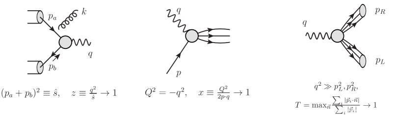
Figure 1: Kinematic definitions for the processes considered in this talk.

In this talk we discuss Drell-Yan (DY) and deep inelastic scattering (DIS) near partonic threshold, and thrust in the two-jet limit (fig. 1). Defining $\hat{s}\equiv(p_{a}+p_{b})^{2}$ the partonic centre of mass energy in DY and $Q^{2}=q^{2}$ the invariant mass of the final state off-shell photon, the partonic threshold is defined by the condition $z\equiv Q^{2}/\hat{s}\to 1$; similarly, assigning momentum $p$ to the incoming parton in DIS, and defining $Q^{2}=-q^{2}$ the invariant mass of the incoming photon, the threshold limit is given by the Bjorken variable $x\equiv Q^{2}/(2p\cdot q)\to 1$. Last, the two-jet limit in thrust is defined by the condition $T={\rm max}_{\vec{n}}\frac{\sum_{i}|\vec{p}_{i}\cdot\vec{n}|}{\sum_{i}|\vec{p}_{i}|}\to 1$, where $\vec{n}$ is the three-vector defining the thrust axis. Labeling collectively the variables $z$, $x$, $T$ by $\xi$, in the limits above the partonic cross section is written as a power expansion in $(1-\xi)\to 0$, with each term developing towers of large logarithms in perturbation theory:

$$\hat{\sigma}(\xi)\sim\sum_{n=0}^{\infty}\bigg{(}\frac{\alpha_{s}}{\pi}\bigg{)}^{n}\Bigg{\{}c_{n}\delta(1-\xi)+\sum_{m=0}^{2n-1}\Bigg{(}c_{nm}\bigg{[}\frac{\ln^{m}(1-\xi)}{1-\xi}\bigg{]}_{+}+d_{nm}\ln^{m}(1-\xi)\Bigg{)}+{\cal O}(1-\xi)\Bigg{\}}.$$ (1)

In this equation the terms $c_{n}$ and $c_{nm}$ represent the leading power (LP) contribution, while the terms $d_{nm}$ give the next-to-leading power (NLP) correction. The towers of large logarithms spoil the convergence of the perturbative series, and need to be resummed. For a long time it has been known how to resum the tower of logarithms in the LP term, see e.g. the seminal papers [1, 2, 3, 4, 5]. Recently, a lot of effort has been devoted to the development of resummation for the towers of logarithms appearing at NLP.

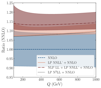
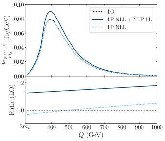
Figure 2: Numerical analysis showing the effect of including resummation of large threshold logarithms at NLP on top of the LP component, in Higgs and di-Higgs production, from [6].

It has been shown (see e.g. [7, 6]) that the resummation of logarithms at NLP may be important for precision physics. For instance, in case of processes such as Drell-Yan and Higgs production in gluon fusion, the resummation of threshold leading logarithms (LL) at NLP gives a contribution of the same order as the tower of next-to-next-to-leading logarithms (NNLL) at LP (fig. 2). Therefore, it would be recommendable for any analysis of particle scattering near threshold with resummation at NN(N)LL accuracy at LP, to include the summation of large logarithms at NLL accuracy at NLP as well.

The development of resummation of NLP logarithms has been investigated both within direct QCD [8, 9, 10, 11, 12, 13, 14, 15, 16, 17, 18, 19, 20, 21, 22, 23, 6, 24, 25, 26, 27, 28, 29, 30, 31, 32, 33, 34, 35], and by means of effective field theory (EFT) methods based on soft-collinear effective field theory (SCET) [36, 37, 38, 39, 40, 41, 42, 43, 44, 45, 46, 47, 7, 48, 49, 50, 51, 52]. In this talk we will summarize recent developments within the second approach.

SCET [53, 54, 55] provides tools to describe soft and collinear radiation systematically, in principle at any subleading power. One introduces soft $q_{s}$, $A_{s}$ and collinear $\xi_{c}$, $A_{c}$ fields, that represent respectively soft and collinear modes of the original QCD fields. Hard modes are integrated out, and appear as short-distance (Wilson) coefficients of effective operators. Let us start by recalling how factorization and resummation is achieved at LP. The effective operators describe the hard scattering kernel of a given process and are written in terms of gauge invariant fields, $\chi_{c}\equiv W_{c}^{{\dagger}}\xi$ for quarks, ${\cal A}_{c}\equiv W_{c}^{{\dagger}}[iD_{c\perp}^{\mu}W_{c}^{{\dagger}}]$ for gluons, where $W_{c}$ is a collinear Wilson line, see e.g. eq. (2.6) of [48] for a definition. Each field is associated with one of the external particles. For instance, the processes in fig. 1 are all described at LP by the current

$$\big{[}\bar{\psi}\gamma_{\mu}\psi\big{]}(0)=\int dt\,d\bar{t}\,\widetilde{C}^{A0}(t,\bar{t})\,J^{A0}_{\mu}(t,\bar{t}),\qquad\qquad J^{A0}_{\mu}(t,\bar{t})=\bar{\chi}_{\bar{c}}(\bar{t}n_{-})\,\gamma_{\perp\mu}\,\chi_{c}(tn_{+}),$$ (2)

where $\widetilde{C}^{A0}(t,\bar{t})$ is the Wilson coefficient in position space. Soft and collinear radiation arises in the effective theory by means of the SCET Lagrangian

$${\cal L}_{\rm SCET}=\sum_{i}{\cal L}_{c_{i}}+{\cal L}_{s}.$$ (3)

Collinear interactions occur within a given collinear sector by means of the collinear Lagrangian ${\cal L}_{c}$; radiation among the different sectors can only be soft and involves the soft Lagrangian ${\cal L}_{s}$. At LP soft-collinear interactions arise only due to a single term in ${\cal L}^{(0)}_{c}$:

$${\cal L}^{(0)}_{c}=\bar{\xi}_{c}\bigg{(}in_{-}D_{c}+g_{s}n_{-}A_{s}(x_{-})+i\not{D}_{\perp c}\frac{1}{in_{+}D_{c}}i\not{D}_{\perp c}\bigg{)}\frac{\not{n}_{+}}{2}\xi_{c}+{\cal L}_{c,\rm YM}^{(0)},$$ (4)

and occur at position $x_{-}$ due to multipole expansion of the soft field in collinear interactions. Furthermore, only the component $n_{-}A_{s}$ appears, which leads to the well-known eikonal Feynman rule $\propto ig_{s}n_{-}^{\mu}$. As it turns out, this interaction can be removed from the Lagrangian by means of a soft-decoupling transformation [54]:

$$\xi(x)\to Y_{+}(x_{-})\xi^{(0)}(x),\qquad\qquad A_{c}^{\mu}(x)\to Y_{+}(x_{-})A_{c}^{(0)\mu}(x)Y_{+}^{{\dagger}}(x_{-}),$$ (5)

where $Y_{+}$ is a soft Wilson line, see e.g. eq. (2.4) of [48], such that one has

$$\bar{\xi}_{c}\Big{(}in_{-}D_{c}+g_{s}n_{-}A_{s}(x_{-})\Big{)}\frac{\not{n}_{+}}{2}\xi_{c}\to\bar{\xi}^{(0)}_{c}\Big{(}in_{-}D^{(0)}_{c}\Big{)}\frac{\not{n}_{+}}{2}\xi^{(0)}_{c}.$$ (6)

This construction guarantees the automatic factorization of a given matrix element (or cross section) into a product of short distance coefficients times collinear and soft functions, defined as matrix elements of gauge-invariant operators made exclusively of collinear and soft fields respectively. In case of the processes in fig. 1 one obtains the factorized expression

$$\frac{d\sigma}{dQ^{2}}=|C^{A0}(Q^{2})|^{2}\times f_{a/A}\otimes f_{b/B}\otimes S_{\rm DY}\big{[}Q(1-z)\big{]},$$ (7)

for the Drell-Yan invariant mass distribution [56],

$$F_{2}=|C^{A0}(Q^{2})|^{2}\times Q^{2}\times f_{a/A}\otimes J_{\overline{hc}}^{(q)}\big{[}Q(1-z)\big{]},$$ (8)

for Deep inelastic scattering [57], and

$$\frac{d\sigma}{d\tau}=|C^{A0}(Q^{2})|^{2}\times J_{c}^{(q)}(p_{L}^{2})\otimes J_{\bar{c}}^{(q)}(p_{R}^{2})\otimes S_{\rm LP}(k),$$ (9)

for thrust [58], with $\tau=1-T$ and $k$ a soft momentum, reproducing older results in QCD [3, 4, 59]. In these equations the matrix elements of (anti-)collinear fields are interpreted either in terms of the parton distribution functions (DY and DIS) or jet functions, (DIS and Thrust), while the soft functions are given as vacuum expectation values of the soft Wilson lines introduced in eq. (5). One of the most important features of the EFT approach is that the original infrared singularities of the scattering amplitude are turned into ultraviolet divergences of the EFT’s operators [60]. The renormalization of such operators provides renormalization group equations (RGEs), whose solution allows one to sum large logarithms associated to the hard, soft and collinear functions, thanks to the fact that within the EFT factorization, these functions are single scale objects.

Let’s now consider the extension of this framework beyond LP. In this respect, one of the advantages of the EFT approach is that every object (fields, derivatives, momenta) has a unique scaling with the small parameter in the problem, conventionally indicated by $\lambda\ll 1$. For instance, in case of Drell-Yan near threshold $\lambda\sim\sqrt{1-z}$. Decomposing momenta along the light-like directions $n_{i\pm}$, such that $p^{\mu}=(n_{+}p)n_{-}^{\mu}/2+p_{\perp}^{\mu}+(n_{-}p)n_{+}^{\mu}/2=(n_{+}p,p_{\perp},n_{-}p)$, collinear and soft momenta have respectively scaling $p_{c}\sim Q(1,\lambda,\lambda^{2})$ and $p_{s}\sim Q(\lambda^{2},\lambda^{2},\lambda^{2})$. In this context, one needs to take into account two sources of power suppression [36, 44, 45]. On the one hand, one has operators that are power suppressed compared to the LP ones in eq. (2). In general, power suppression is achieved either by inserting transverse derivatives, $\partial_{\perp}\sim\lambda$, or by adding more collinear fields along the same collinear direction. It is also possible to insert gauge-invariant combinations of soft fields, but these contribute in general beyond NLP. Starting from the LP current in eq. (2) we have e.g.

$$\bar{\chi}_{\bar{c}}(\bar{t}n_{-})\,\gamma_{\perp}^{\mu}\,\chi_{c}(tn_{+})\,\, \to \,\,\bar{\chi}_{\bar{c}}(\bar{t}n_{-})\big{[}n_{\pm}^{\mu}\,i\not{\partial}_{\perp}\big{]}\chi_{c}(tn_{+}),\hskip 49.79231pt\mbox{(A1-type),}$$

$$\searrow \,\,\bar{\chi}_{\bar{c}}(\bar{t}n_{-})\big{[}n_{\pm}^{\mu}\,\not{\cal A}_{c\perp}(t_{2}n_{+})\big{]}\chi_{c}(t_{1}n_{+}),\hskip 14.22636pt\mbox{(B1-type),}$$ (10)

where for the labeling of power suppressed operators we refer to [44, 45]. The operators on the r.h.s of eq. (1) are suppressed by one power of $\lambda$ compared to the operator on the l.h.s. Given that $\lambda\sim\sqrt{1-z}$, in general one needs to take into account operators suppressed up to two powers of $\lambda$, in order to reproduce a given cross section up to NLP. The second source of power suppression originates by considering time-ordered products of LP operators with power-suppressed insertions of terms from the SCET Lagrangian. Given the collinear SCET Lagrangian ${\cal L}_{c}={\cal L}^{(0)}_{c}+{\cal L}^{(1)}_{c}+{\cal L}^{(2)}_{c}+{\cal O}(\lambda^{3})$, one has e.g. two terms contributing to ${\cal L}^{(1)}_{c}$ [61], given by

$${\cal L}^{(1)\rm gluon}_{c}=\bar{\xi}\Big{[}x_{\perp}^{\mu}n_{-}^{\nu}W_{c}g_{s}F_{\mu\nu}^{s}(x_{-})W_{c}^{{\dagger}}\Big{]}\frac{\not{n_{+}}}{2}\xi,\qquad{\cal L}^{(1)\rm quark}_{c}=\bar{q}(x_{-})W_{c}^{{\dagger}}i\not{D}_{\perp c}\xi,$$ (11)

where the first term involves the emission of a soft gluon and in the second a collinear quark is converted into a soft quark, upon emission of a collinear gluon. Now, the difference compared to our previous discussion of factorization at LP is that soft-collinear interactions at subleading power, such as the one in eq. (11), are not removed by the decoupling transformation eq. (5). Formally it is still possible to proceed with the factorization of a given matrix element into its soft and collinear components. However, a few differences arise compared to the factorization theorems at LP.

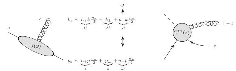
Figure 3: Convolutions appearing at NLP between jet and soft functions (left, see e.g. [46, 48]) or between short-distance coefficients and jet functions (right, see e.g. [49]).

When the power suppression is given by a soft-collinear Lagrangian insertion such as in eq. (11), we obtain a convolution between a collinear and a soft function, where the convolution variable is related to the small component of the collinear momentum, which is of the same order of the corresponding component of the soft momentum, (fig. 3, left diagram), and therefore cannot be integrated out. This factorization structure appear for instance in Drell-Yan [46, 48]. When the power suppression is given by the insertion of an operator involving two or more particle in the same collinear sector, such as the B1 type operator in eq. (1), convolution between the corresponding short-distance coefficient and jet function arises, where the convolution variable is related to the fraction of collinear momentum shared between the two particle in the same collinear sector (fig. 3, right diagram). This factorization structure arise for instance in off-diagonal DIS [49].

2 Endpoint divergences at NLP

The presence of convolutions does not constitute a problem per se. However, as it turns out, these integrations are often divergent in $d=4$. For instance, in case of DY one finds [48]

$$\int d\omega\,J(\omega)\,S(\omega)\sim\int_{0}^{\Omega}d\omega\,\underbrace{(n_{+}p\omega)^{-\epsilon}}_{\rm collinear\,\,piece}\underbrace{\frac{1}{\omega^{1+\epsilon}}\frac{1}{(\Omega-\omega)^{\epsilon}}}_{\rm soft\,\,piece}\bigg{|}_{\Omega=Q(1-z)},$$ (12)

which for $\epsilon\to 0$ is divergent for $\omega\to 0$. In case of off-diagonal scalar DIS [49] one finds

$$\int dz\,C^{B1}(z)\,J_{qg}(z)\sim\int_{0}^{1}dz\,\underbrace{\bigg{(}\frac{\mu^{2}}{s_{qg}z\bar{z}}\bigg{)}^{\epsilon}}_{\rm collinear\,\,piece}\underbrace{\frac{\alpha_{s}C_{F}}{2\pi}\frac{(1-z)^{2}}{z}}_{\rm hard\,\,piece}\bigg{|}_{s_{qg}=Q^{2}\frac{1-x}{x}},$$ (13)

which for $\epsilon\to 0$ diverges for $z\to 0$. In order to investigate the structure of these endpoint divergences, let’s consider the case of DIS more in detail: In eq. (13) we have inserted the Wilson coefficient at tree level. At one loop one has [49]

$$C^{B1}(z)\Big{|}_{\rm 1\,\,loop} \sim C^{B1}(z)\Big{|}_{\rm tree}\frac{\alpha_{s}}{\pi}\frac{1}{\epsilon^{2}}\bigg{\{}{\bf T}_{1}\cdot{\bf T}_{0}\bigg{(}\frac{\mu^{2}}{zQ^{2}}\bigg{)}^{\epsilon}+{\bf T}_{2}\cdot{\bf T}_{0}\bigg{(}\frac{\mu^{2}}{\bar{z}Q^{2}}\bigg{)}^{\epsilon}$$ (14)

$$\hskip 71.13188pt+\,{\bf T}_{1}\cdot{\bf T}_{2}\bigg{[}\bigg{(}\frac{\mu^{2}}{Q^{2}}\bigg{)}^{\epsilon}-\bigg{(}\frac{\mu^{2}}{zQ^{2}}\bigg{)}^{\epsilon}\bigg{]}\bigg{\}}+{\cal O}(\epsilon^{-1})$$

The term $\propto{\bf T}_{1}\cdot{\bf T}_{2}$ contains a single pole, which however gives rise to a leading pole after integration. The correct result is obtained only within dimensional regularization:

$$\frac{1}{\epsilon^{2}}\int_{0}^{1}dz\,\frac{1}{z^{1+\epsilon}}(1-z^{-\epsilon})=-\frac{1}{2\epsilon^{3}},$$ (15)

while expanding for $\epsilon\to 0$ leads to nonsense results:

$$\frac{1}{\epsilon^{2}}\int_{0}^{1}dz\,\frac{1}{z^{1+\epsilon}}\bigg{(}\epsilon\ln z-\frac{\epsilon^{2}}{2!}\ln^{2}z+\frac{\epsilon^{3}}{3!}\ln^{3}z+\ldots\bigg{)}=-\frac{1}{\epsilon^{3}}+\frac{1}{\epsilon^{3}}-\frac{1}{\epsilon^{3}}+\ldots.$$ (16)

This poses a problem for standard resummation techniques. As discussed above, within an EFT approach one renormalizes the collinear and soft matrix elements, obtaining a set of RGEs whose solution resums the large logarithms. From eqs. (12), (13) and (14), however, it is clear that not all logarithms are generated within the hard, soft and jet functions themselves: an additional pole (and thus a corresponding logarithm) is generated through the endpoint divergent convolution. Closer inspection of eq. (14) reveals that the endpoint divergence actually points a break of the EFT itself (fig. 4):

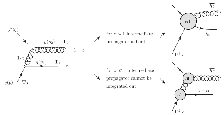
Figure 4: Structure of endpoint divergence in off-diagonal scalar DIS, from [49].

The factor $1/z$ in the Wilson coefficient $C^{B1}$ is due to the intermediate gluon propagator (l.h.s. of fig. 4). For generic $z\sim 1$, this propagator is hard, thus an EFT description in terms of a short-distance Wilson coefficient is appropriate (upper r.h.s. of fig. 4). However, $z$ is integrated in the range (0,1), and when $z\ll 1$, the intermediate propagator is not hard, and cannot be integrated out: the correct EFT description is now given by the lower diagram on the r.h.s. of fig. 4. For $z\ll 1$ the short-distance coefficient $C^{B1}$ becomes a two-scale object, and together with the corresponding power-suppressed operator it refactorizes into a jet function times the LP Wilson coefficient and operator $C^{A0}$ [49]:

$$C^{B1}(Q,z)J^{B1}\stackrel{{\scriptstyle z\to 0}}{{\longrightarrow}}C^{A0}(Q^{2})\int d^{4}x\,T\Big{[}J^{A0},{\cal L}^{(1)\rm quark}_{z-\overline{sc}}\Big{]}=C^{A0}(Q^{2})D^{B1}(zQ^{2})J^{B1}_{z-\overline{sc}},$$ (17)

where on the r.h.s. $C^{A0}(Q^{2})$ and $D^{B1}(zQ^{2})$ can now be interpreted correctly as single-scale function. Such refactorization has been observed also in other applications of SCET to the analysis of processes at NLP, such as $H\to\gamma\gamma$, $H\to gg$ [62, 63, 64, 65].

The analysis of DIS shows that a correct EFT treatment needs to take into account both the configurations appearing on the r.h.s. of fig. 4. Once both contributions are taken into account, one expects endpoint divergences to cancel between the two terms. In case of DIS, such construction involves the factorization of the perturbative part of the initial state PDF, which makes the construction more involved. In the next section we will focus instead on off-diagonal thrust, where the cancellation of endpoint divergences can be shown explicitly, without involving initial-state singularities.

3 NLP LLs in Thrust in the two-jet limit

Let us consider thrust in the two-jet limit: following [51], we consider the power-suppressed contribution given by the process (fig. 5)

$$e^{+}e^{-}\to\gamma^{*}\to[g]_{c}+[q\bar{q}]_{\bar{c}}.$$ (18)

Within SCET this process is given by two contributions [51]: a “direct” term (B-type) (first diagram on the left in fig. 6) and a time ordered product involving a soft quark emission (A-type) (two diagrams on the right in fig. 6): the former involves the matrix element

$$\langle X_{c}|\langle X_{\bar{c}}|\langle X_{s}|\,\bar{\chi}_{\bar{c}}(\bar{t}_{1}n_{-})\Gamma_{i}^{\mu\nu}\mathcal{A}_{c\perp\nu}(tn_{+})\chi_{\bar{c}}(\bar{t}_{2}n_{-})\,|0\rangle\,,$$ (19)

with $i=1,2$ representing two different strings of Dirac matrices, while the latter stems from the matrix element

$$\langle X_{c}|\langle X_{\bar{c}}|\langle X_{s}|\int d^{d}x\,T\,[\bar{\chi}_{c}(tn_{+})\gamma_{\perp}^{\mu}\chi_{\bar{c}}(\bar{t}n_{-}),i{\cal L}^{(1)\rm quark}_{c}(x)]\,|0\rangle\,.$$ (20)

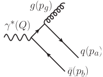
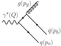
Figure 5: Off-diagonal “gluon” thrust in the two-jet limit. Figure from [51].

Inserting these matrix elements in the corresponding cross section, one finds that the “direct” B-type term factorizes into a hard, (anti-)collinear and soft functions, according to

$$\frac{1}{\sigma_{0}}\frac{d\sigma}{dM_{R}^{2}dM_{L}^{2}}\bigg{|}_{\rm B-type} \sim \frac{2C_{F}}{Q^{2}}f(\epsilon)\int_{0}^{\infty}dl_{+}dl_{-}\,\sum_{i,i^{\prime}=1,2}\int drdr^{\prime}\,C^{\rm B1*}_{i^{\prime}}(Q^{2},r^{\prime})C^{\rm B1}_{i}(Q^{2},r)$$ (21)

$$\times\,\bigg{\{}\,\delta_{ii^{\prime}}\,\mathcal{J}_{\bar{c}}^{q\bar{q}(8)}(M_{R}^{2}-Ql_{+},r,r^{\prime})+\,\ldots\bigg{\}}\,\mathcal{J}_{c}^{(g)}(M_{L}^{2}-Ql_{-})\,S^{(g)}(l_{+},l_{-})\,,$$

where

$$f(\epsilon)=\bigg{(}\frac{Q^{2}}{4\pi}\bigg{)}^{-\epsilon}\frac{(1-\epsilon)^{2}\Gamma(1-\epsilon)}{\Gamma(2-2\epsilon)},$$ (22)

and the ellipses represent regular terms not important for our analysis below. Due to the fact that $C^{\rm B1}_{i}(r)\sim 1/r$, eq. (21) develops endpoint divergences when the quark ($r\to 0$) or the anti-quark ($r\to 1$) become soft:

$$\frac{1}{\sigma_{0}}\frac{d\sigma}{dM_{R}^{2}dM_{L}^{2}}\bigg{|}_{\rm B-type}\sim\int_{0}^{1}dr\,\bigg{[}\frac{1}{r^{1+\epsilon}}+\frac{1}{(1-r)^{1+\epsilon}}\bigg{]}\,.$$ (23)

On the other hand, the A-type matrix element of eq. (20) gives rise to the factorized cross section

$$\frac{1}{\sigma_{0}}\frac{d\sigma}{dM_{R}^{2}dM_{L}^{2}}|_{\rm A-type} \sim \frac{2C_{F}}{Q}\,|C^{\rm A0}(Q^{2})|^{2}\int_{0}^{\infty}dl_{+}dl_{-}\,\int d\omega d\omega^{\prime}\,\mathcal{J}_{\bar{c}}^{(\bar{q})}(M_{R}^{2}-Ql_{+})$$ (24)

$$\times\,\bigg{\{}\,\mathcal{J}_{c}(M_{L}^{2}-Ql_{-},\omega,\omega^{\prime})\,S_{\rm NLP}(l_{+},l_{-},\omega,\omega^{\prime})+\ldots\bigg{\}}\,,$$

which develops endpoint divergences when the soft quark or anti-quark become energetic ($\omega\to\infty$):

$$\frac{1}{\sigma_{0}}\frac{d\sigma}{dM_{R}^{2}dM_{L}^{2}}|_{\rm A-type}\sim 2\int_{M_{R}^{2}/Q}^{\infty}d\omega\,\frac{1}{\omega^{1+\epsilon}}\,.$$ (25)

As for DIS, in the $r\to 0$ (or $r\to 1$) limit the coefficients $C_{i}^{B1}$ become a two-scale object, and refactorize according to

$$C_{1}^{\rm B1}(Q^{2},r) \stackrel{{\scriptstyle r\to 0}}{{=}} C^{\rm A0}(Q^{2})\times\frac{D^{\rm B1}(rQ^{2})}{r}+\mathcal{O}(r^{0})\,,$$

$$C_{2}^{\rm B1}(Q^{2},r) \stackrel{{\scriptstyle r\to 1}}{{=}} -C^{\rm A0}(Q^{2})\times\frac{D^{\rm B1}(\bar{r}Q^{2})}{\bar{r}}+\mathcal{O}(\bar{r}^{0})\,.$$ (26)

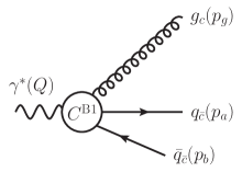
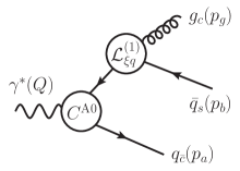
Figure 6: Matrix elements in SCET corresponding respectively to eq. (19) (first diagram on the left) and eq. (20) (second and third diagrams). Diagrams from [51].

Furthermore, we expect that endpoint divergences should cancel when summing the A and B-type contributions, which in turn implies that in the asymptotic limits $r,r^{\prime}\to 0(1)$, $\omega,\omega^{\prime}\to\infty$, the integrands of the A- and B-type terms should become identical. While it is easy to check that this is indeed what happens at lowest order in perturbation theory, in general this gives a series of refactorization conditions [51], which are summarized graphically in fig. 7: starting from the A-type term (upper left diagram in fig. 7), in the limit $\omega,\omega^{\prime}\to\infty$ the soft (anti)-quark becomes energetic, thus we get to the lower left diagram in fig. 7, provided that [51]

(I) $$\hskip 14.22636pt\mathcal{J}_{c}\left(p^{2},\omega,\omega^{\prime}\right)=\mathcal{J}_{c}^{(g)}(p^{2})\,\displaystyle\frac{D^{\rm B1}(\omega Q)}{\omega}\frac{{D^{\rm B1}}^{*}(\omega^{\prime}Q)}{\omega^{\prime}}+\mathcal{O}\!\left(\frac{1}{\omega^{(\prime)}}\right)\,,$$ (27)

where the function $D^{\rm B1}(p^{2})$ is the same as the one appearing in the factorization of the hard B1 operator coefficient (3). On the other hand, starting from the B-type term (lower right diagram in fig. 7), in the limit $r,r^{\prime}\to 0(1)$ the anticollinear (anti-)quark becomes soft, thus we get to the upper right diagram in fig. 7, provided that eq. (3) holds. At this point, the requirement that the integrands of the A- and B-type terms should become identical in the asymptotic limits $r,r^{\prime}\to 0(1)$, $\omega,\omega^{\prime}\to\infty$, (i.e., that the lower left- and the upper right-diagram in fig. 7 should coincide), gives the last refactorization condition: in Laplace space one has [51]

$$\mbox{(II)}\quad Q\,\widetilde{\mathcal{J}}^{(\bar{q})}_{\bar{c}}(s_{R})\,\widetilde{S}_{\rm NLP}\left(s_{R},s_{L},\omega,\omega^{\prime}\right)\Big{|}_{\omega^{(\prime)}\to\infty}=\widetilde{\mathcal{J}}^{q\bar{q}(8)}_{\bar{c}}\left(s_{R},r,r^{\prime}\right)\widetilde{S}^{(g)}(s_{R},s_{L})\Big{|}_{r^{(\prime)}=\omega^{(\prime)}/Q\to 0}\,,$$ (28)

and the same identity holds with $r,r^{\prime}\to\bar{r},\bar{r}^{\prime}$.

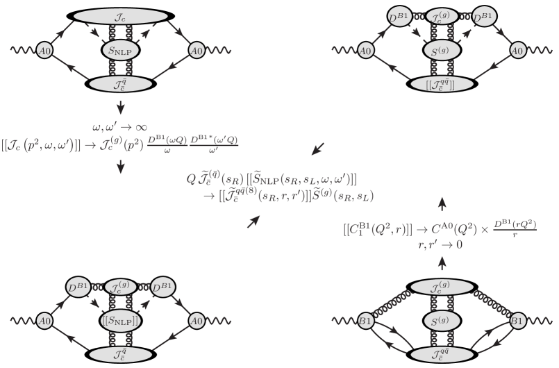
Figure 7: Consistency conditions necessary to achieve refactorization and the cancellation of endpoint divergences, as obtained in [51].

The constraint that in the asymptotic limits the A- and B-type terms must coincide provides also a method to deal with endpoint divergences. Let us define the asymptotic limits of the various function by using a double-bracket notation: for instance, in functions of $\omega,\omega^{\prime}$, we rescale $\omega\to\kappa\omega$, $\omega^{\prime}\to\kappa\omega^{\prime}$ and take $\kappa\to\infty$. Then

$$\llbracket S_{\rm NLP}\left(l_{+},l_{-},\omega,\omega^{\prime}\right)\rrbracket\equiv S_{\rm NLP}\left(l_{+},l_{-},\omega,\omega^{\prime}\right)|_{\mathcal{O}(\kappa^{0})},$$ (29)

$$\llbracket\mathcal{J}_{c}(p^{2},\omega,\omega^{\prime})\rrbracket\equiv\mathcal{J}_{c}(p^{2},\omega,\omega^{\prime})|_{\mathcal{O}(\kappa^{-2})}\,,$$ (30)

where $\delta(\omega-\omega^{\prime})$ counts as $\kappa^{-1}$. A similar notation is used in functions of $r,r^{\prime}$ and we refer to [51] for a precise definition. As discussed above, endpoint divergences arise in the asymptotic limits, where the A- and B-type terms take the factorized form given respectively in the left lower graph of fig. 7, and right upper graph of fig. 7: the cancellation of endpoint divergences requires these two limits to be identical, therefore we can introduce the integral

$$\frac{2C_{F}}{Q}\,f(\epsilon)\,|C^{\rm A0}(Q^{2})|^{2}\widetilde{\mathcal{J}}^{(\bar{q})}_{\bar{c}}(s_{R})\widetilde{\mathcal{J}}_{c}^{(g)}(s_{L})$$

$$\times\int_{0}^{\infty}d\omega d\omega^{\prime}\,\frac{D^{\rm B1}(\omega Q)}{\omega}\frac{D^{\rm B1*}(\omega^{\prime}Q)}{\omega^{\prime}}\left\llbracket\widetilde{S}_{\rm NLP}(s_{R},s_{L},\omega,\omega^{\prime})\right\rrbracket,\qquad$$ (31)

which is scaleless over the whole domain and thus vanishes in $d$ dimensions, but it can be shown to reproduce respectively the endpoint divergences of the A- and B-type contribution, when splitting the integration into two domains $I_{2}$ and $I_{1}$, as represented in fig. 8 [51]. Thus it is possible to remove the endpoint divergences from both the A- and B-type contributions by subtracting the integrand in eq. (31) integrated over region $I_{2}$ from the A-type term, and by subtracting eq. (31) integrated over region $I_{1}$ from the B-type term. The subtracted expressions are now separately endpoint-finite, but depend on $\Lambda$. However, as long as no approximations are made, the $\Lambda$ dependence cancels exactly between the two terms. After some elaboration [51] the endpoint finite A-term can be written as

$$\frac{1}{\sigma_{0}}\frac{\widetilde{d\sigma}}{ds_{R}ds_{L}}|_{\rm A-type} = \frac{2C_{F}}{Q}\,f(\epsilon)\,|C^{\rm A0}(Q^{2})|^{2}\,\widetilde{\mathcal{J}}_{\bar{c}}^{(\bar{q})}(s_{R})\,\int d\omega d\omega^{\prime}\,\Big{[}1-\theta(\omega-\Lambda)\theta(\omega^{\prime}-\Lambda)\Big{]}$$ (32)

$$\times\,\bigg{\{}\,\widetilde{\mathcal{J}}_{c}(s_{L},\omega,\omega^{\prime})\,\widetilde{S}_{\rm NLP}(s_{R},s_{L},\omega,\omega^{\prime})+\,\widetilde{\!\!\widehat{\mathcal{J}}}_{\!c}(s_{L},\omega,\omega^{\prime})\,\,\widetilde{\!\widehat{S}}_{\rm NLP}(s_{R},s_{L},\omega,\omega^{\prime})\bigg{\}}\,,\qquad$$

where the equality signs hold up to corrections of $\mathcal{O}(1/(s_{L}\Lambda),1/(s_{R}\Lambda))$, and the and B-type term takes the form

$$\frac{1}{\sigma_{0}}\frac{\widetilde{d\sigma}}{ds_{R}ds_{L}}|_{\scriptsize\begin{array}[]{l}$\rm B--type$\\[-2.84544pt] $i=i'=1$\end{array}} = \frac{2C_{F}}{Q^{2}}\,f(\epsilon)\,\widetilde{\mathcal{J}}_{c}^{(g)}(s_{L})\,\widetilde{S}^{(g)}(s_{R},s_{L})$$ (36)

$$\times\,\bigg{\{}\int_{0}^{1}drdr^{\prime}\,\big{[}1-\theta(\Lambda/Q-r)\theta(\Lambda/Q-r^{\prime})\big{]}\,C^{\rm B1*}_{1}(Q^{2},r^{\prime})C^{\rm B1}_{1}(Q^{2},r)\,\widetilde{\mathcal{J}}_{\bar{c}}^{q\bar{q}(8)}(s_{R},r,r^{\prime})\quad$$

$$-\int_{0}^{\infty}drdr^{\prime}\,\big{[}\theta(r-\Lambda/Q)\theta(\Lambda/Q-r^{\prime})+\theta(\Lambda/Q-r)\theta(r^{\prime}-\Lambda/Q)\big{]}\,$$

$$\times\,\llbracket C^{\rm B1*}_{1}(Q^{2},r^{\prime})\rrbracket_{0}\,\llbracket C^{\rm B1}_{1}(Q^{2},r)\rrbracket_{0}\,\llbracket\widetilde{\mathcal{J}}_{\bar{c}}^{q\bar{q}(8)}(s_{R},r,r^{\prime})\rrbracket_{0}\,\bigg{\}}\,,$$

up to corrections of $\mathcal{O}(\Lambda/Q)$. It is now possible to use these expressions to develop the resummation of large logarithms with standard methods, and we refer to [51] for a detailed discussion of such derivation.

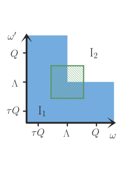
Figure 8: Visual representation of the regions $I_{1}$ and $I_{2}$, used to construct subtraction terms as described in the text. In the overlap region in green the asymptotic behaviour of the A- and B-type term must agree. Figure from [51].

4 NLP NNLO in Drell-Yan near threshold

The analysis of off-diagonal thrust has allowed us to fully appreciate the nature of endpoint divergences: these are indeed an artifact of the effective field theory, which arise due to how the original (phase space or loop) integrations in QCD are split among the different regions of the effective theory. When all momentum regions are correctly taken into account, (A- and B-type terms in case of off-diagonal thrust), endpoint divergences cancel. This allows one to devise the construction of subtraction terms such as to make the individual contributions finite. Formally, the finite factorization formulas such as eqs. (32) and (36) are expected to be valid at all orders in perturbation theory and at any logarithmic accuracy. However, for off-diagonal thrust the explicit construction has been obtained at LL accuracy. In order to go beyond this logarithmic order, in general one needs to calculate the factorized matrix elements beyond leading order in perturbation theory. In turn, this would allow one to check explicitly that the refactorization conditions such as those in eqs. (27) and (28) hold to higher order in perturbation theory.

With this goal in mind, a set of papers [48, 50, 52] have been dedicated to calculate the full set of collinear and soft functions necessary to reproduce the Drell-Yan invariant mass distribution at NLP near threshold, up to NNLO in perturbation theory. In particular, this requires the calculation of the collinear functions up to one loop and the soft function up to two loops. Let us focus for simplicity on the off diagonal $\bar{q}g$ channel. In [52] the factorization theorem has been obtained formally at all subleading power. Writing the invariant mass distribution as

$$\frac{d\sigma_{\rm DY}}{dQ^{2}}=\sigma_{0}\sum_{a,b}\int_{\tau}^{1}\,\frac{dz}{z}\,{\cal L}_{ab}\bigg{(}\frac{\tau}{z}\bigg{)}\,\Delta_{ab}(z)+\mathcal{O}\left(\frac{\Lambda}{Q}\right),\qquad\sigma_{0}=\frac{4\pi\alpha_{\rm em}^{2}}{3N_{c}Q^{2}s},$$ (37)

where the parton luminosity function ${\cal L}_{ab}(y)$ is defined as

$${\cal L}_{ab}(y)=\int_{y}^{1}\frac{dx}{x}\,f_{a/A}(x)\,f_{b/B}\bigg{(}\frac{y}{x}\bigg{)},$$ (38)

up to NLP the partonic cross section factorizes as follows:

$$\Delta_{g\bar{q}}|_{\rm NLP}(z)=8H(Q^{2})\,\int{d\omega}\,d\omega^{\prime}\,G^{*}_{\xi q}(x_{a}n_{+}p_{A};\omega^{\prime})\,G_{\xi q}(x_{a}n_{+}p_{A};\omega)\,S(\Omega,\omega,\omega^{\prime})\,,$$ (39)

where $G_{\xi q}$, $G^{*}_{\xi q}$ are collinear function appearing respectively in the amplitude and complex conjugate amplitude, $H(Q^{2})=|C^{A0}(Q^{2})|^{2}$ is the hard function, and $S(\Omega,\omega,\omega^{\prime})$ the soft function. The collinear function coincides with the function $D^{B1}$ in eqs. (3) and (27). Indeed, this collinear matrix element appears to be a “universal” function appearing in the context of several factorization theorems at NLP; for instance, it appears also in the context of $H\to\gamma\gamma$, [62], and it has been calculated up to two loops in [66]. At one loop it reads

$${G}^{(1)}_{\xi q}\left(n_{+}p;\omega\right) = -\,\frac{\alpha_{s}}{4\pi}\big{(}C_{F}-C_{A}\big{)}\left(\frac{n_{+}p\,\omega}{\mu^{2}}\right)^{-\epsilon}\frac{2-4\epsilon-\epsilon^{2}}{2\epsilon^{2}}\frac{e^{\epsilon\gamma_{E}}\Gamma[1+\epsilon]\Gamma[{1-\epsilon}]^{2}}{\Gamma[{2-2\epsilon}]}$$

$$= -\,\frac{\alpha_{s}}{4\pi}\big{(}C_{F}-C_{A}\big{)}\bigg{[}\frac{1}{\epsilon^{2}}-\frac{1}{\epsilon}\ln\left(\frac{n_{+}p\,\omega}{\mu^{2}}\right)-\,\frac{1}{2}-\frac{\pi^{2}}{12}+\frac{1}{2}\ln^{2}\left(\frac{n_{+}p\,\omega_{1}}{\mu^{2}}\right)+\mathcal{O}(\epsilon)\bigg{]}\,.$$

The soft function at one loop reads

$$S_{g\bar{q}}^{(1)}(\Omega,\omega,\omega^{\prime})=\frac{\alpha_{s}\,T_{F}}{4\pi}\frac{e^{\epsilon\gamma_{E}}}{\Gamma[1-\epsilon]}\frac{1}{\omega}\bigg{(}\frac{\mu^{2}}{\omega\,(\Omega-\omega)}\bigg{)}^{\epsilon}\delta(\omega-\omega^{\prime})\,\theta(\Omega-\omega)\theta(\omega),$$ (41)

where the color factor $T_{F}$ is given in terms of the relation ${\rm Tr}[{\bf T}^{A}{\bf T}^{B}]=T_{F}\,\delta^{AB}=\delta^{AB}/2$. The two loop contribution is quite involved. It includes a virtual-real and a real-real contributions

$$S^{(2)}_{g\bar{q}}(\Omega,\omega,\omega^{\prime})=S^{(2)1r1v}_{g\bar{q}}(\Omega,\omega,\omega^{\prime})+S^{(2)2r0v}_{g\bar{q}}(\Omega,\omega,\omega^{\prime}),$$ (42)

which individually read

$$S^{(2)1r1v}_{g\bar{q}}(\Omega,\omega,\omega^{\prime}) = \frac{\alpha_{s}^{2}\,T_{F}}{(4\pi)^{2}}(2C_{F}-C_{A})\frac{e^{2\epsilon\gamma_{E}}\,\Gamma[1+\epsilon]}{\epsilon\,\Gamma[1-\epsilon]}$$ (43)

$$\times\,{\rm Re}\bigg{\{}\frac{1}{(-\omega)\omega^{\prime}}\bigg{[}\frac{\omega+\omega^{\prime}}{\omega^{\prime}}\,_{2}F_{1}\bigg{(}1,1+\epsilon,1-\epsilon,\frac{\omega}{\omega^{\prime}}\bigg{)}-1\bigg{]}\bigg{(}\frac{\mu^{4}}{(-\omega)\omega^{\prime}(\Omega-\omega^{\prime})^{2}}\bigg{)}^{\epsilon}\theta(-\omega)$$

$$+\,\frac{2(\omega+\omega^{\prime})}{\omega\omega^{\prime}(\omega^{\prime}-\omega)}\bigg{(}\frac{\mu^{4}}{(\omega^{\prime}-\omega)^{2}(\Omega-\omega^{\prime})^{2}}\bigg{)}^{\epsilon}\frac{\Gamma[1-\epsilon]^{2}}{\Gamma[1-2\epsilon]}\theta(\omega^{\prime}-\omega)\bigg{\}}\theta(\omega^{\prime})\theta(\Omega-\omega^{\prime}),$$

and

$$S^{(2)2r0v}_{g\bar{q}}(\Omega,\omega,\omega^{\prime}) = \frac{\alpha_{s}^{2}T_{F}}{(4\pi)^{2}}\bigg{\{}C_{F}\frac{e^{2\epsilon\gamma_{E}}\Gamma[1-\epsilon]}{\epsilon^{2}}\frac{1}{\omega}\bigg{[}\frac{4}{\Gamma[1-3\epsilon]}\bigg{(}\frac{\mu^{4}}{\omega(\Omega-\omega)^{3}}\bigg{)}^{\epsilon}$$

$$+\,\frac{(4-\epsilon)\Gamma[2-\epsilon]}{(1-2\epsilon)\Gamma[1-2\epsilon]^{2}}\bigg{(}\frac{\mu^{4}}{\omega^{2}(\Omega-\omega)^{2}}\bigg{)}^{\epsilon}\bigg{]}\delta(\omega-\omega^{\prime})\theta(\Omega-\omega)\theta(\omega)$$

$$+\,\left(C_{A}-2C_{F}\right)\frac{2e^{2\epsilon\gamma_{E}}}{\epsilon\Gamma[1-2\epsilon]}\frac{\omega+\omega^{\prime}}{\omega\omega^{\prime}(\omega^{\prime}-\omega)}\bigg{(}\frac{\mu^{4}}{\omega(\omega^{\prime}-\omega)(\Omega-\omega^{\prime})^{2}}\bigg{)}^{\epsilon}$$

$$\times\,\bigg{[}\,_{2}F_{1}\Big{(}1,-\epsilon,1-\epsilon,\frac{\omega}{\omega-\omega^{\prime}}\Big{)}-1\bigg{]}\theta(\omega)\theta(\omega^{\prime})\theta(\omega^{\prime}-\omega)\theta(\Omega-\omega^{\prime})\bigg{\}}.$$

With these results at hand one can now study the structure of endpoint divergences in the asymptotic limits $\omega,\omega^{\prime}\to 0$, and we refer to [52] for further details.

5 Outlook

The resummation of large logarithms at NLP poses interesting theoretical challenges. Within an effective field theory approach based on SCET it is possible to systematically factorize the effect of soft and collinear radiation in physical observables. In this talk we have discussed the derivation of factorization theorems for scattering processes such as Drell-Yan and deep inelastic scattering near threshold, and thrust in the two-jet limit. In general, once bare factorization theorems have been derived, the subsequent step of obtaining the resummation of large logarithms by means of a RGE approach is made nontrivial by the appearance of endpoint divergences [48, 49]. It has been shown that these are an artifact of the effective theory. Endpoint divergences cancel among terms in the factorization theorems, once all contributions are correctly taken into account. It is then possible to devise a subtraction procedure, which makes the individual contributions finite, thus allowing the application of standard RGE procedure. This approach has been fully developed to obtain the resummation of large logarithms in off-diagonal “gluon thrust” at LL accuracy [51]. In order to extend resummation at NLP to higher logarithmic accuracy more data is needed. To this end one needs to calculate collinear and soft functions appearing in the factorization theorems at higher order in perturbation theory. This program has been completed for Drell-Yan near threshold in a series of papers, [48, 50, 52], where all collinear and soft functions have been calculated respectively at one and two loops in perturbation theory.

References

- [1] G. Parisi, Summing Large Perturbative Corrections in QCD, Phys. Lett. B 90 (1980) 295–296.
- [2] G. Curci and M. Greco, Large infrared corrections in QCD processes, Phys. Lett. B92 (1980) 175–178.
- [3] G. Sterman, Summation of large corrections to short distance hadronic cross-sections, Nucl. Phys. B281 (1987) 310.
- [4] S. Catani and L. Trentadue, Resummation of the QCD perturbative series for hard processes, Nucl. Phys. B327 (1989) 323.
- [5] S. Catani and L. Trentadue, Comment on qcd exponentiation at large x, Nucl. Phys. B353 (1991) 183–186.
- [6] M. van Beekveld, E. Laenen, J. Sinninghe Damsté and L. Vernazza, Next-to-leading power threshold corrections for finite order and resummed colour-singlet cross sections, JHEP 05 (2021) 114, [2101.07270].
- [7] M. Beneke, M. Garny, S. Jaskiewicz, R. Szafron, L. Vernazza and J. Wang, Leading-logarithmic threshold resummation of Higgs production in gluon fusion at next-to-leading power, JHEP 01 (2020) 094, [1910.12685].
- [8] E. Laenen, L. Magnea and G. Stavenga, On next-to-eikonal corrections to threshold resummation for the Drell-Yan and DIS cross sections, Phys. Lett. B669 (2008) 173–179, [0807.4412].
- [9] E. Laenen, G. Stavenga and C. D. White, Path integral approach to eikonal and next-to-eikonal exponentiation, JHEP 0903 (2009) 054, [0811.2067].
- [10] E. Laenen, L. Magnea, G. Stavenga and C. D. White, Next-to-eikonal corrections to soft gluon radiation: a diagrammatic approach, JHEP 1101 (2011) 141, [1010.1860].
- [11] D. Bonocore, E. Laenen, L. Magnea, L. Vernazza and C. D. White, The method of regions and next-to-soft corrections in Drell-Yan production, Phys. Lett. B742 (2015) 375–382, [1410.6406].
- [12] D. Bonocore, E. Laenen, L. Magnea, S. Melville, L. Vernazza and C. D. White, A factorization approach to next-to-leading-power threshold logarithms, JHEP 06 (2015) 008, [1503.05156].
- [13] D. Bonocore, E. Laenen, L. Magnea, L. Vernazza and C. D. White, Non-abelian factorisation for next-to-leading-power threshold logarithms, JHEP 12 (2016) 121, [1610.06842].
- [14] V. Del Duca, E. Laenen, L. Magnea, L. Vernazza and C. D. White, Universality of next-to-leading power threshold effects for colourless final states in hadronic collisions, JHEP 11 (2017) 057, [1706.04018].
- [15] H. Gervais, Soft photon theorem for high energy amplitudes in Yukawa and scalar theories, Phys. Rev. D95 (2017) 125009, [1704.00806].
- [16] N. Bahjat-Abbas, J. Sinninghe Damsté, L. Vernazza and C. D. White, On next-to-leading power threshold corrections in Drell-Yan production at N3LO, JHEP 1810 (2018) 144, [1807.09246].
- [17] N. Bahjat-Abbas, D. Bonocore, J. Sinninghe Damsté, E. Laenen, L. Magnea, L. Vernazza et al., Diagrammatic resummation of leading-logarithmic threshold effects at next-to-leading power, JHEP 11 (2019) 002, [1905.13710].
- [18] M. van Beekveld, W. Beenakker, E. Laenen and C. D. White, Next-to-leading power threshold effects for inclusive and exclusive processes with final state jets, JHEP 03 (2020) 106, [1905.08741].
- [19] M. van Beekveld, W. Beenakker, R. Basu, E. Laenen, A. Misra and P. Motylinski, Next-to-leading power threshold effects for resummed prompt photon production, Phys. Rev. D 100 (2019) 056009, [1905.11771].
- [20] E. Laenen, J. Sinninghe Damsté, L. Vernazza, W. Waalewijn and L. Zoppi, Towards all-order factorization of QED amplitudes at next-to-leading power, Phys. Rev. D 103 (2021) 034022, [2008.01736].
- [21] D. Bonocore, Asymptotic dynamics on the worldline for spinning particles, JHEP 02 (2021) 007, [2009.07863].
- [22] D. Bonocore, A. Kulesza and J. Pirsch, Classical and quantum gravitational scattering with Generalized Wilson Lines, JHEP 03 (2022) 147, [2112.02009].
- [23] D. Bonocore and A. Kulesza, Soft photon bremsstrahlung at next-to-leading power, Phys. Lett. B 833 (2022) 137325, [2112.08329].
- [24] M. van Beekveld, L. Vernazza and C. D. White, Threshold resummation of new partonic channels at next-to-leading power, JHEP 12 (2021) 087, [2109.09752].
- [25] N. Agarwal, M. van Beekveld, E. Laenen, S. Mishra, A. Mukhopadhyay and A. Tripathi, Next-to-leading power corrections to event shape variables, 2306.17601.
- [26] A. Ajjath, P. Mukherjee and V. Ravindran, On next to soft corrections to Drell-Yan and Higgs Boson productions, 2006.06726.
- [27] A. H. Ajjath, P. Mukherjee, V. Ravindran, A. Sankar and S. Tiwari, On next to soft threshold corrections to DIS and SIA processes, JHEP 04 (2021) 131, [2007.12214].
- [28] A. H. Ajjath, P. Mukherjee, V. Ravindran, A. Sankar and S. Tiwari, Next-to-soft corrections for Drell-Yan and Higgs boson rapidity distributions beyond N3LO, Phys. Rev. D 103 (2021) L111502, [2010.00079].
- [29] A. H. Ajjath, P. Mukherjee, V. Ravindran, A. Sankar and S. Tiwari, Next-to-soft-virtual resummed rapidity distribution for the Drell-Yan process to , Phys. Rev. D 106 (2022) 034005, [2112.14094].
- [30] A. H. Ajjath, P. Mukherjee, V. Ravindran, A. Sankar and S. Tiwari, Next-to SV resummed Drell–Yan cross section beyond leading-logarithm, Eur. Phys. J. C 82 (2022) 234, [2107.09717].
- [31] A. H. Ajjath, P. Mukherjee, V. Ravindran, A. Sankar and S. Tiwari, Resummed Higgs boson cross section at next-to SV to , Eur. Phys. J. C 82 (2022) 774, [2109.12657].
- [32] A. H. Ajjath, P. Mukherjee and V. Ravindran, Going beyond soft plus virtual, Phys. Rev. D 105 (2022) L091503, [2204.09012].
- [33] T. Engel, A. Signer and Y. Ulrich, Universal structure of radiative QED amplitudes at one loop, JHEP 04 (2022) 097, [2112.07570].
- [34] T. Engel, The LBK theorem to all orders, JHEP 07 (2023) 177, [2304.11689].
- [35] M. Czakon, F. Eschment and T. Schellenberger, Subleading Effects in Soft-Gluon Emission at One-Loop in Massless QCD, 2307.02286.
- [36] A. J. Larkoski, D. Neill and I. W. Stewart, Soft theorems from effective field theory, JHEP 1506 (2015) 077, [1412.3108].
- [37] I. Moult, L. Rothen, I. W. Stewart, F. J. Tackmann and H. X. Zhu, Subleading power corrections for N-jettiness subtractions, Phys. Rev. D95 (2017) 074023, [1612.00450].
- [38] I. Moult, I. W. Stewart and G. Vita, A subleading operator basis and matching for gg H, JHEP 1707 (2017) 067, [1703.03408].
- [39] I. Moult, L. Rothen, I. W. Stewart, F. J. Tackmann and H. X. Zhu, N -jettiness subtractions for at subleading power, Phys. Rev. D97 (2018) 014013, [1710.03227].
- [40] M. A. Ebert, I. Moult, I. W. Stewart, F. J. Tackmann, G. Vita and H. X. Zhu, Power Corrections for N-Jettiness Subtractions at , JHEP 12 (2018) 084, [1807.10764].
- [41] I. Moult, I. W. Stewart, G. Vita and H. X. Zhu, First Subleading Power Resummation for Event Shapes, JHEP 08 (2018) 013, [1804.04665].
- [42] I. Moult, I. W. Stewart and G. Vita, Subleading Power Factorization with Radiative Functions, 1905.07411.
- [43] I. Moult, I. W. Stewart, G. Vita and H. X. Zhu, The Soft Quark Sudakov, JHEP 05 (2020) 089, [1910.14038].
- [44] M. Beneke, M. Garny, R. Szafron and J. Wang, Anomalous dimension of subleading-power N-jet operators, JHEP 03 (2018) 001, [1712.04416].
- [45] M. Beneke, M. Garny, R. Szafron and J. Wang, Anomalous dimension of subleading-power -jet operators. Part II, JHEP 11 (2018) 112, [1808.04742].
- [46] M. Beneke, A. Broggio, M. Garny, S. Jaskiewicz, R. Szafron, L. Vernazza et al., Leading-logarithmic threshold resummation of the Drell-Yan process at next-to-leading power, JHEP 1903 (2019) 043, [1809.10631].
- [47] M. Beneke, M. Garny, R. Szafron and J. Wang, Violation of the Kluberg-Stern-Zuber theorem in SCET, JHEP 09 (2019) 101, [1907.05463].
- [48] M. Beneke, A. Broggio, S. Jaskiewicz and L. Vernazza, Threshold factorization of the Drell-Yan process at next-to-leading power, JHEP 07 (2020) 078, [1912.01585].
- [49] M. Beneke, M. Garny, S. Jaskiewicz, R. Szafron, L. Vernazza and J. Wang, Large-x resummation of off-diagonal deep-inelastic parton scattering from d-dimensional refactorization, JHEP 10 (2020) 196, [2008.04943].
- [50] A. Broggio, S. Jaskiewicz and L. Vernazza, Next-to-leading power two-loop soft functions for the Drell-Yan process at threshold, JHEP 10 (2021) 061, [2107.07353].
- [51] M. Beneke, M. Garny, S. Jaskiewicz, J. Strohm, R. Szafron, L. Vernazza et al., Next-to-leading power endpoint factorization and resummation for off-diagonal “gluon” thrust, JHEP 07 (2022) 144, [2205.04479].
- [52] A. Broggio, S. Jaskiewicz and L. Vernazza, Threshold factorization of the Drell-Yan quark-gluon channel and two-loop soft function at next-to-leading power, JHEP 12 (2023) 028, [2306.06037].
- [53] C. W. Bauer, S. Fleming, D. Pirjol and I. W. Stewart, An effective field theory for collinear and soft gluons: Heavy to light decays, Phys. Rev. D63 (2001) 114020, [hep-ph/0011336].
- [54] C. W. Bauer, D. Pirjol and I. W. Stewart, Soft collinear factorization in effective field theory, Phys. Rev. D 65 (2002) 054022, [hep-ph/0109045].
- [55] M. Beneke, A. P. Chapovsky, M. Diehl and T. Feldmann, Soft collinear effective theory and heavy to light currents beyond leading power, Nucl. Phys. B 643 (2002) 431–476, [hep-ph/0206152].
- [56] T. Becher, M. Neubert and G. Xu, Dynamical Threshold Enhancement and Resummation in Drell-Yan Production, JHEP 07 (2008) 030, [0710.0680].
- [57] T. Becher, M. Neubert and B. D. Pecjak, Factorization and Momentum-Space Resummation in Deep-Inelastic Scattering, JHEP 01 (2007) 076, [hep-ph/0607228].
- [58] T. Becher and M. D. Schwartz, A precise determination of from LEP thrust data using effective field theory, JHEP 07 (2008) 034, [0803.0342].
- [59] S. Catani, L. Trentadue, G. Turnock and B. R. Webber, Resummation of large logarithms in e+ e- event shape distributions, Nucl. Phys. B407 (1993) 3–42.
- [60] T. Becher and M. Neubert, On the Structure of Infrared Singularities of Gauge-Theory Amplitudes, JHEP 0906 (2009) 081, [0903.1126].
- [61] M. Beneke and T. Feldmann, Multipole expanded soft collinear effective theory with nonAbelian gauge symmetry, Phys. Lett. B 553 (2003) 267–276, [hep-ph/0211358].
- [62] Z. L. Liu and M. Neubert, Factorization at subleading power and endpoint-divergent convolutions in decay, JHEP 04 (2020) 033, [1912.08818].
- [63] Z. L. Liu, B. Mecaj, M. Neubert and X. Wang, Factorization at subleading power, Sudakov resummation, and endpoint divergences in soft-collinear effective theory, Phys. Rev. D 104 (2021) 014004, [2009.04456].
- [64] Z. L. Liu, B. Mecaj, M. Neubert and X. Wang, Factorization at subleading power and endpoint divergences in decay. Part II. Renormalization and scale evolution, JHEP 01 (2021) 077, [2009.06779].
- [65] Z. L. Liu, M. Neubert, M. Schnubel and X. Wang, Factorization at next-to-leading power and endpoint divergences in gg → h production, JHEP 06 (2023) 183, [2212.10447].
- [66] Z. L. Liu, M. Neubert, M. Schnubel and X. Wang, Radiative quark jet function with an external gluon, JHEP 02 (2022) 075, [2112.00018].