DPoser: Diffusion Model as Robust 3D Human Pose Prior

Abstract

Modeling human pose is a cornerstone in applications from human-robot interaction to augmented reality, yet crafting a robust human pose prior remains a challenge due to biomechanical constraints and diverse human movements. Traditional priors like VAEs and NDFs often fall short in realism and generalization, especially in extreme conditions such as unseen noisy poses. To address these issues, we introduce DPoser, a robust and versatile human pose prior built upon diffusion models. Designed with optimization frameworks, DPoser seamlessly integrates into various pose-centric applications, including human mesh recovery, pose completion, and motion denoising. Specifically, by formulating these tasks as inverse problems, we employ variational diffusion sampling for efficient solving. Furthermore, acknowledging the disparity between the articulated poses we focus on and structured images in previous research, we propose a truncated timestep scheduling to boost performance on downstream tasks. Our exhaustive experiments demonstrate DPoser’s superiority over existing state-of-the-art pose priors across multiple tasks.

1 Introduction

The accurate modeling of human pose is an essential building block in a variety of applications, ranging from human-robot interaction to augmented and virtual reality experiences. Many real-world applications rely on a prior distribution of valid human poses to perform tasks like body model fitting, motion capture, and gesture recognition. Existing methods use Gaussian Mixture Models (GMMs) [34], Variational Autoencoders (VAEs) [35], or Neural Distance Fields (NDFs) [36] to model the complex human pose prior. However, these models have limitations. GMMs can generate implausible poses due to their unbounded nature, VAEs are constrained by Gaussian assumptions, and NDFs exhibit limited generalization capabilities, requiring additional training strategies for extreme poses. These shortcomings underscore the need for a more robust and reliable human pose prior, a gap that this work aims to fill.

Diffusion models [10, 8, 12, 14] have recently gained traction for their prowess in capturing complex, high-dimensional data distributions and enabling versatile sampling techniques. Although they have been employed in specialized applications like generating realistic human motion sequences [45, 46] or serving as multi-hypothesis pose estimators based on 2D inputs [41, 43], their utility has generally been constrained. These models are designed for generation or tailored to work with specific types of input data, which limits their applicability in broader contexts. Thus far, the potential of diffusion models as a universal human pose prior remains largely untapped, and effective optimization methods for diverse applications remain unanswered.

In this work, we propose DPoser, a novel approach that leverages time-dependent denoiser learned from expansive motion capture datasets to construct a robust human pose prior. Specifically, by viewing various pose-centric tasks as inverse problems, we propose to employ variational diffusion sampling techniques [18] to incorporate DPoser as a regularization term within the existing optimization framework e.g., SMPLify [34]. Furthermore, our experimental investigations into the generative aspects of articulated human poses reveal that the major information during diffusion is concentrated on the “clean” end of the perturbed data, as opposed to the entire noise-to-clean trajectory. Motivated by this insight, we introduce a truncated annealed timestep scheduling for optimization, which demonstrates superior efficiency over conventional random and full annealed schedules across multiple downstream tasks.

In summary, our main contributions of this work can be summarized as follows:

• We introduce DPoser, a novel framework based on diffusion models to craft a robust and flexible human pose prior, geared for seamless integration across diverse pose-related applications via test-time optimization.

• Utilizing a fresh perspective on inverse problems, we employ variational diffusion sampling during test-time optimization and introduce truncated timestep scheduling, showing superior efficiency over traditional methods.

• Through extensive experiments and ablation studies, we establish that DPoser not only outshines state-of-the-art (SOTA) pose priors in a variety of applications but also provides valuable insights into training techniques such as suitable rotation representations for peak performance.

2 Related works

2.1 Human Pose Priors

Human body models such as SMPL [33] serve as powerful tools for parameterizing both pose and shape, thereby offering a comprehensive framework for describing a wide array of human gestures. Within the SMPL model, body poses are captured using rotation matrices or joint angles linked to a kinematic skeleton. Adjusting these parameters enables the representation of a diverse range of human actions. However, due to inherent biomechanical constraints, plausible poses inherently reside in a lower-dimensional manifold.

Numerous approaches [34, 35, 36] have been proposed to model this intrinsic pose prior. Classical generative models like GMMs, VAEs [16], and GANs [17] have been employed to capture the complex underlying distribution, demonstrating significant improvements in downstream tasks such as human mesh recovery [49, 50]. Additionally, some research has explored task-specific conditional pose priors, augmenting the model with additional inputs like image features [42, 48], 2D joint coordinates [43], or preceding poses in motion sequences [40, 39]. Our work adopts the unconditional pose prior framework. We train DPoser on large-scale motion capture datasets without auxiliary inputs like paired images or captions, to ensure its applicability across a broad spectrum of pose-related tasks.

2.2 Diffusion Models for Pose-centric Tasks

Diffusion models [6, 8, 10, 11] have emerged as powerful tools for capturing intricate data distributions, aligning particularly well with the demands of multi-hypothesis estimation in ambiguous human poses. Notable works include DiffPose [41], which leverages a Gaussian Mixture Model-guided forward diffusion process [58] and employs a Graph Convolutional Network (GCN) [57] architecture conditioned on 2D pose sequences for 3D pose estimation by learned reverse process (i.e., generation). In a similar vein, DiffusionPose [42] and GFPose [43] employ the generation-based pipeline but take different approaches in conditioning. ZeDO [44] focuses on 2D-to-3D pose lifting, while works like Diff-HMR [48] and DiffHand [47] extend to estimating SMPL parameters and hand mesh vertices. BUDDI [62] stands out for using diffusion models to capture the joint distribution of interacting individuals and leveraging SDS loss [27, 28] for test-time optimization.

Our work, DPoser, parallels BUDDI in similar optimization implementation. However, we distinguish ourselves by introducing a wider perspective of inverse problems and proposing advanced timestep scheduling based on characteristics of human poses. Moreover, DPoser is designed to work as a flexible regularization term, making it adaptable to diverse pose-centric tasks. It should also be noted that unlike most works [44, 42, 43, 41] that focus on joint positions, DPoser targets the more complex issue of joint rotations, adding an extra layer of challenge due to the intricacy of rotation representations.

3 Preliminary: Score-based Diffusion Models

Diffusion models [3, 6, 8, 10] operationalize generative processes by inverting a predefined forward diffusion process, typically formulated as a linear stochastic differential equation (SDE). Formally, the data trajectory $\left\{\mathbf{x}(t)\in\mathbb{R}^{n}\right\}_{t\in[0,1]}$ follows the forward SDE given by:

$$\mathrm{d}\mathbf{x}=\mu(t)\mathbf{x}\mathrm{d}t+g(t)\mathrm{d}\mathbf{w}.$$ (1)

Here, $\mu(t)\mathbf{x}\in\mathbb{R}^{n}$ and $g(t)\in\mathbb{R}$ represent the drift and diffusion coefficients, while $\mathbf{w}$ is a standard Wiener process.

The affine drift coefficients ensure analytically tractable Gaussian perturbation kernels, denoted by $p_{0t}(\mathbf{x}_{t}\mid\mathbf{x})=\mathcal{N}(\mathbf{x}_{t};\alpha_{t}\mathbf{x},\sigma_{t}^{2}\mathbf{I})$, where the exact coefficients $\alpha_{t},\sigma_{t}$ can be obtained with standard techniques [7]. Using appropriately designed $\alpha_{t}$ and $\sigma_{t}$, this allows the data distribution $\mathbf{x}_{0}\sim p_{data}$ to morph into a tractable isotropic Gaussian distribution $\mathbf{x}_{1}\sim\mathcal{N}(\mathbf{0},\mathbf{I})$ via forward diffusion.

To recover data distribution $p_{data}$ from the Gaussian distribution $\mathcal{N}(\mathbf{0},\mathbf{I})$, we can simulate the corresponding reverse SDE of Eq. (1) [8]:

$$\mathrm{d}\mathbf{x}=[\mu(t)\mathbf{x}-g(t)^{2}\nabla_{\mathbf{x}_{t}}\log p_{t}\left(\mathbf{x}_{t}\right)]\mathrm{d}t+g(t)\mathrm{d}\bar{\mathbf{w}}.$$ (2)

The so-called score function [4], $\nabla_{\mathbf{x}_{t}}\log p_{t}\left(\mathbf{x}_{t}\right)$, serves as an unknown term in Eq. (2) and can be approximated by a neural network parameterized as $\epsilon_{\theta}(\mathbf{x}_{t};t)\approx-\sigma_{t}\nabla_{\mathbf{x}_{t}}\log p_{t}\left(\mathbf{x}_{t}\right)$. To learn the score functions, employing denoising score matching techniques [2], we first introduce noise to the data points as per:

$$\mathbf{x}_{t}=\alpha_{t}\mathbf{x}_{0}+\sigma_{t}\epsilon,\epsilon\sim\mathcal{N}(\mathbf{0},\mathbf{I}).$$ (3)

Subsequently, we train the time-dependent noise predictor $\epsilon_{\theta}(\mathbf{x}_{t};t)$ using an L2-loss defined as [10]:

$$\mathbb{E}_{\mathbf{x}_{0}\sim p_{\mathrm{data}},\epsilon\sim\mathcal{N}(\mathbf{0},\mathbf{I}),t\sim\mathcal{U}[0,1]}\left[w(t)||\epsilon-\epsilon_{\theta}(\mathbf{x}_{t};t)||_{2}^{2}\right],$$ (4)

where $w(t)$ denotes a positive weighting function. Upon successful training, the score functions can be estimated and used to solve the reverse SDE (Eq. (2)). Through techniques like Euler-Maruyama discretization, we can generate novel samples by simulating the reverse SDE.

4 Methods

4.1 Learning Pose Prior with Diffusion Models

We propose to model pose prior based on the SMPL body model [33], which can be viewed as a differentiable function $[J,V]=M(\theta,\beta)$ that maps body joint angles $\theta\in\mathbb{R}^{3\times 21}$ and shape parameters $\beta\in\mathbb{R}^{10}$ to mesh vertices $V\in\mathbb{R}^{3\times 6890}$ and joint positions $J\in\mathbb{R}^{3\times 22}$. Our target is to model the distribution of joint angles $p(\theta)$. To achieve this, we train DPoser on mocap datasets, employing sub-VP SDEs introduced in ScoreSDE [8], defined as:

$$\mathrm{d}\mathbf{x}=-\frac{1}{2}\beta(t)\mathbf{x}\mathrm{d}t+\sqrt{\beta(t)(1-e^{-2\int_{0}^{t}\beta(s)\mathrm{d}s})}\mathrm{d}\mathbf{w},$$ (5)

where $\beta(t)$ denotes linear scheduled noise scales. The coefficients needed in Eq. (3) can be obtained as $\alpha_{t}=e^{-\frac{1}{2}\int_{0}^{t}\beta(s)\mathrm{d}s},\sigma_{t}=[1-e^{-\int_{0}^{t}\beta(s)\mathrm{d}s}]^{2}$. With the constructed forward process (Eq. (3)) to sample $\mathbf{x}_{t}$, we then apply the objective in Eq. (4) to train the noise predictor $\epsilon_{\theta}(\mathbf{x}_{t};t)$ with weights $w(t)=\sigma_{t}^{2}$ as suggested in ScoreSDE [8].

In our experiments, we find the selection of rotation representations, such as axis-angle and 6D rotations [59], to be crucial for optimal performance when coupled with suitable normalization. Despite experimenting with incorporating body models via auxiliary losses, as in prior work [35, 39], we note that it imposes a computational burden without evident gains in downstream task performance. Further methodological nuances are detailed in the Appendix.

4.2 Optimization Leveraging Diffusion Priors

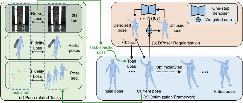
Figure 2: Overview of the DPoser Methodology. Panel (a) presents three tasks: human mesh recovery, pose completion, and motion denoising, with omissions like camera optimization and bending loss for clarity. Panel (b) demonstrates the DPoser regularization process, introducing noise to the current pose and applying a one-step denoiser to achieve a denoised pose. $L_{\text{DPoser}}$ is computed between the denoised and current pose. Panel (c) outlines the optimization process from initial to current and fitted poses via loss minimization.

The acquired score functions or noise predictors, denoted as $\epsilon_{\theta}(\mathbf{x}_{t};t)$, permit the direct generation of plausible poses through Eq. (2). Yet, the broader integration of diffusion priors into general optimization frameworks remains an open avenue. We address this by reframing pose-related tasks as inverse problems and applying variational diffusion sampling techniques [18] for efficient resolution.

Inverse problem formulation. Consider an original signal $\mathbf{x}_{0}$. Inverse problems can be encapsulated by Eq. (6) as:

$$\mathbf{y}=\mathcal{A}(\mathbf{x}_{0})+\mathbf{n},\quad\mathbf{y},\mathbf{n}\in\mathbb{R}^{d},~{}\mathbf{x}_{0}\in\mathbb{R}^{n},$$ (6)

where $\mathcal{A}$ symbolizes the measurement operator and $\mathbf{n}$ constitutes noise, assumed to be white Gaussian $\mathcal{N}(\mathbf{0},\sigma_{n}^{2}\mathbf{I})$ in our context. As an illustration, inverse kinematics can be considered as inferring joint rotations (or body poses in SMPL [33]) from observed joint positions. Moreover, the 2D-3D lifting task can be modeled as a linear inverse problem, with $\mathcal{A}$ representing a camera projection model. To recover the original signal $\mathbf{x}_{0}$, in the Bayesian framework, our target is to sample from the posterior distribution $p\left(\mathbf{x}_{0}\mid\mathbf{y}\right)$.

Diffusion-based inverse problem solving. Various techniques [26, 21, 19, 20, 22, 18] have been explored to simulate this posterior sampling process based on diffusion priors. For some noiseless linear inverse problems, such as completion, alternating projections onto measurement subspaces are commonly employed [8, 21, 20]. For instance, in hand pose completion, a standard iterative generation process using diffusion models can be applied, replacing known parts of the pose at each iteration.

However, such projections are inconvenient to build general optimization frameworks concerned in our work. To navigate these challenges, we adopt variational diffusion sampling [18], efficient in computation and straightforward in implementation. Specifically, it employs a variational distribution $q\left(\mathbf{x}_{0}\mid\mathbf{y}\right):=\mathcal{N}(\mu,\sigma^{2}\mathbf{I})$ and aims to minimize the Kullback-Leibler (KL) divergence between this variational distribution and the true posterior, mathematically expressed as $KL\big{(}q\left(\mathbf{x}_{0}\mid\mathbf{y}\right)\parallel p\left(\mathbf{x}_{0}\mid\mathbf{y}\right)\big{)}$.

Informed by existing theorems concerning the likelihood properties of diffusion models [9], and under the assumption of zero variance ($\sigma\approx 0$), the optimization problem of seeking $\mathbf{x}_{0}$ (i.e., $\mu$) can be formulated as minimizing [18]:

$$\|\mathbf{y}-\mathcal{A}(\mathbf{x}_{0})\|^{2}+w_{t}(\mathtt{sg}[\epsilon_{\theta}(\mathbf{x}_{t};t)-\epsilon])^{\top}\mathbf{x}_{0},$$ (7)

where $w_{t}$ denotes the loss weights and $\epsilon$ is sampled from the standard Gaussian distribution. Here, $\mathtt{sg}$ signifies the stopped-gradient operator, indicating that backpropagation through the trained diffusion models is not required. The optimization procedure initiates by selecting a timestep $t$ and applying a perturbation to the target $\mathbf{x}_{0}$ as per Eq. (3), resulting in $\mathbf{x}_{t}$. Subsequently, the gradients $[\epsilon_{\theta}(\mathbf{x}_{t};t)-\epsilon]$ are applied to the optimization variable $\mathbf{x}_{0}$. In a nutshell, this framework [18] provides a flexible yet robust strategy for employing diffusion priors in generic optimization problems, serving as a cornerstone for our work.

DPoser regularization. To shed more light on the working mechanism, we reformulate the regularization term as:

$$L_{\mathrm{DPoser}} =w_{t}||\mathbf{x}_{0}-\mathtt{sg}[\mathbf{\hat{x}}_{0}(t)]||_{2}^{2},\text{where}$$ (8)

$$\mathbf{\hat{x}}_{0}(t) =\frac{\mathbf{x}_{t}-\sigma_{t}\epsilon_{\theta}(\mathbf{x}_{t};t)}{\alpha_{t}}.$$ (9)

Here, $\mathbf{\hat{x}}_{0}(t)$ serves as a one-step denoised estimate, leveraging the trained diffusion model $\epsilon_{\theta}(\mathbf{x}_{t};t)$. We show that the gradient of our DPoser regularization aligns with Eq. (7).

Proof: Differentiating Eq. (8) with respect to $\mathbf{x}_{0}$ yields:

$$\nabla_{\mathbf{x}_{0}}L_{\mathrm{DPoser}} =2w_{t}(\mathbf{x}_{0}-\mathbf{\hat{x}}_{0}(t))$$

$$=2w_{t}(\frac{\mathbf{x}_{t}-\sigma_{t}\epsilon}{\alpha_{t}}-\frac{\mathbf{x}_{t}-\sigma_{t}\epsilon_{\theta}(\mathbf{x}_{t};t)}{\alpha_{t}})$$

$$=2w_{t}\frac{\sigma_{t}}{\alpha_{t}}(\epsilon_{\theta}(\mathbf{x}_{t};t)-\epsilon)$$

$$\propto(\epsilon_{\theta}(\mathbf{x}_{t};t)-\epsilon).$$ (10)

Therefore, our DPoser regularization $L_{\mathrm{DPoser}}$ can be implemented as an L2-loss. In this view, during optimization, DPoser works by pulling the current pose $\mathbf{x}_{0}$ closer to the learned plausible pose distribution through denoising.

DPoser across pose-related tasks. Capitalizing on DPoser’s inherent flexibility, we adapt it to various human pose tasks, with a spotlight on human mesh recovery as illustrated in Fig. 2. For an exhaustive examination of DPoser’s utility across different pose-related applications including pose completion and motion denoising, we direct the reader to our Appendix.

By adapting the objective function from the SMPLify framework [34], we supplant the originally used GMM prior with our own DPoser regularization term, $L_{\mathrm{DPoser}}$, while also forgoing the intricate interpenetration error term. The optimization objective, incorporating both pose $\theta$ and shape $\beta$ parameters in SMPL [33], is articulated as:

$$L(\theta,\beta)=L_{J}+w_{\theta}L_{\theta}+w_{\beta}L_{\beta}+w_{\alpha}L_{\mathrm{DPoser}}.$$ (11)

Herein, the reprojection loss $L_{J}$ serves as the data fidelity term, mathematically expressed as:

$$L_{J} =\sum_{i\in\text{Joints}}\lambda_{i}\rho\left(\Pi_{C}\left(M_{J}(\theta,\beta)_{i}\right)-J^{\text{est}}_{i}\right),$$ (12)

where $M_{J}(\theta,\beta)$ and $\Pi_{C}$ symbolize the 3D joint positions regressed from SMPL and the 3D-to-2D camera projection function, respectively. $J^{\text{est}}$ are the 2D keypoints estimated using an off-the-shelf 2D pose estimator (OpenPose [60] in our experiments), and $\lambda_{i}$ indicates the confidence score of joint $i$. The Geman-McClure error function [61] $\rho$ serves to robustly quantify discrepancies in 2D joint positions.

The bending term $L_{\theta}$ is incorporated to penalize excessive bending at the elbows and knees, formulated as $L_{\theta}=\sum_{i\in\text{(elbows, knees)}}\exp(\boldsymbol{\theta}_{i})$. The shape regularizer $L_{\beta}$ is a simple L2 norm, i.e., $L_{\beta}=\|\beta\|_{2}^{2}$. The constant weights for prior terms are denoted as $w_{\theta},w_{\beta}$ and $w_{\alpha}$, respectively.

Contrasting SMPLify’s GMM-based prior, we employ $L_{\mathrm{DPoser}}$ to draw the pose closer to our learned manifold. Given the structure of $L_{\mathrm{DPoser}}$ (as seen in Eq. (8)), a crucial aspect lies in judiciously selecting the diffusion timestep $t$ during the iterative optimization process. We address this concern by introducing our novel truncated timestep scheduling strategy in the subsequent section.

4.3 Test-time Truncated Timestep Scheduling

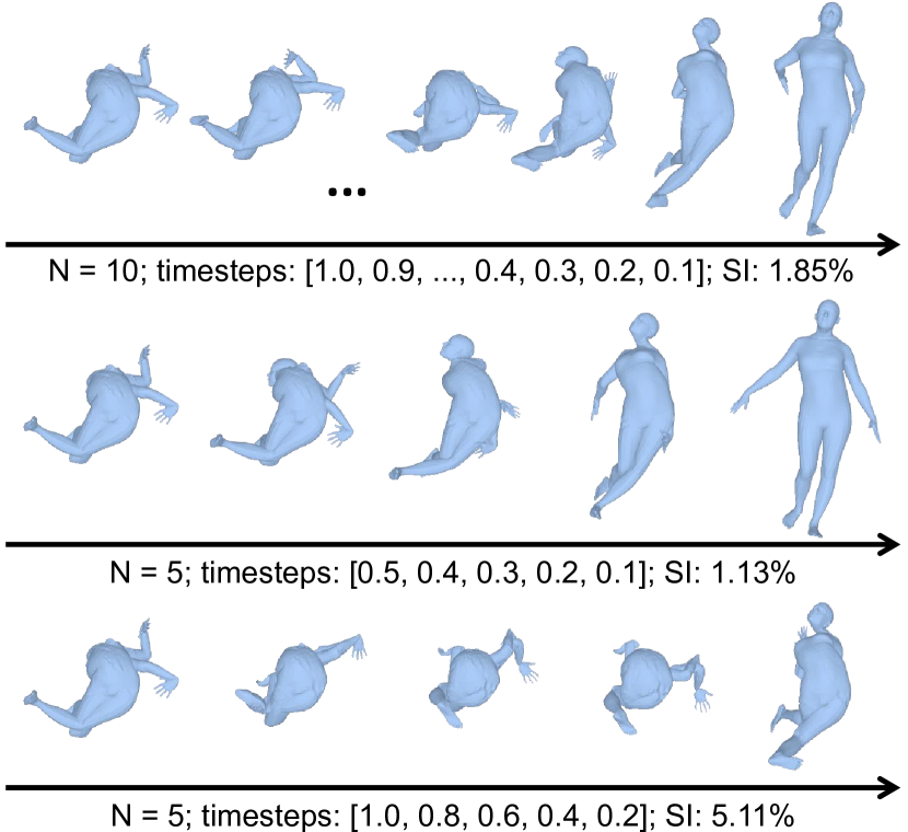
Figure 3: Illustration of the rationale behind our proposed truncated timestep scheduling. We employ the deterministic DDIM sampler [11] with limited steps and assess the quality of generated poses using the Self-Intersection percentage (SI).

Algorithm 1 Test-time Optimization with DPoser

1:A trained diffusion model $\epsilon_{\theta}(\mathbf{x}_{t};t)$, task-specific loss $L_{\text{task}}$, range of diffusion timesteps $[t_{\text{max}},t_{\text{min}}]$, number of optimization iterations $N$, DPoser weights $w_{t}$

2:Initialization of parameters $\mathbf{x}_{0}$

3:for $\text{iter}=0,1,\ldots,N-1$ do

4:     $t\leftarrow t_{\text{max}}-\frac{(t_{\text{max}}-t_{\text{min}})\times\text{iter}}{N-1}$ $\triangleright$ Timestep scheduling

5:     Sample $\epsilon\sim\mathcal{N}(0,I)$

6:     $\mathbf{x}_{t}\leftarrow\alpha_{t}\mathbf{x}_{0}+\sigma_{t}\epsilon$ $\triangleright$ Forward diffusion

7:     $\mathbf{\hat{x}}_{0}(t)\leftarrow\frac{\mathbf{x}_{t}-\sigma_{t}\epsilon_{\theta}(\mathbf{x}_{t};t)}{\alpha_{t}}$ $\triangleright$ One-step denoiser

8:     $L_{\text{DPoser}}\leftarrow w_{t}\lVert\mathbf{x}_{0}-\text{sg}[\mathbf{\hat{x}}_{0}(t)]\rVert_{2}^{2}$

9:     $L_{\text{total}}\leftarrow L_{\text{task}}+L_{\text{DPoser}}$

10:     Update $\mathbf{x}_{0}$ via backpropagation on $L_{\text{total}}$

11:end for

12:return $\mathbf{x}_{0}$

Insights from pose generation. In optimizing pose-related tasks, one fundamental challenge arises from the gap between the image-based data and the articulated pose parameters we manipulate. Prior studies in image domains [15] have noted that earlier timesteps (i.e., smaller $t$) are typically aligned with perceptual content, while the later timesteps are more closely associated with the refinement of details in the diffusion process. As illustrated in Fig. 3, our experimental foray into employing diffusion models for pose generation yields an interesting insight into pose domains: the concentration of meaningful information resides at the “clean” side of the diffusion trajectory, rather than being dispersed uniformly from noise to clean states. This observation serves as the catalyst for our introduction of a truncated annealed timestep scheduling mechanism.

Truncated timestep scheduling. Departing from traditional diffusion models that uniformly sample across the continuum from $1.0$ to $0.0$, we introduce a selective sampling strategy. Specifically, we truncate the timestep range to intervals such as $0.2\to 0$, thereby focusing on the data segments most laden with meaningful information. Based on the linear annealed scheduling, the truncated timestep $t$ for each optimization step can be formulated as:

$$t=t_{\text{max}}-\frac{(t_{\text{max}}-t_{\text{min}})\times\text{iter}}{N-1}.$$ (13)

Here, $N$ signifies the total optimization iterations, while iter represents the current optimization iteration. We summarize our DPoser optimization framework as Algorithm 1, where the truncated range $[t_{\text{max}},t_{\text{min}}]$ is typically set to $[0.2,0.001]$.

Through ablation studies, we prove that the proposed truncated timestep scheduling offers significant advantages over the random, fixed, and full annealed ones utilized in previous works [62, 18, 19, 8], delivering more efficient optimization across a wide range of downstream tasks. This is achieved by concentrating computation on the most informative portions of the data trajectory, as informed by our preliminary sampling investigations on pose generation.

5 Experiments

In this section, we first elaborate on the implementation details and evaluation metrics. We showcase the robustness and versatility of DPoser across a spectrum of pose-centric applications, including pose generation, human mesh recovery, pose completion, and motion denoising. Additionally, we conduct an ablation study to delve into the key elements contributing to our model’s performance.

Sample source	APD $\uparrow$	SI $\downarrow$
Real-world (AMASS) [52]	15.44	0.79
GMM [34]	16.28	1.54
VPoser [35]	10.75	1.51
Pose-NDF [36]	18.75	1.97
DPoser (ours)	14.28	1.21
DPoser (ours)*	19.03	1.13

Table 1: Comparative analysis of pose generation metrics. The discrepancy between visual impressions and APD/SI metrics is discussed, with reference to Fig. 4. *Indicates the use of a DDIM sampler [11] with a reduced 10-step discretization.

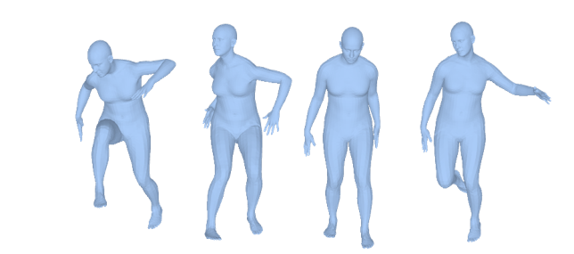
(a) AMASS samples

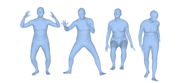
(b) DPoser (ours)

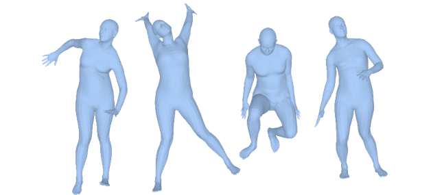
(c) DPoser (ours)*

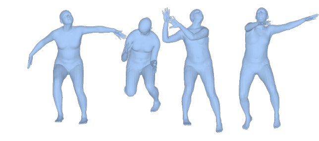
(d) GMM

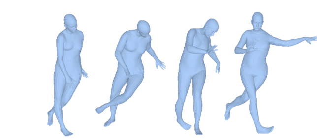
(e) Pose-NDF

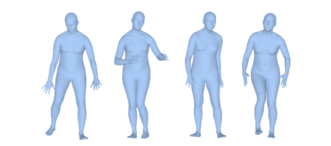
(f) VPoser

Figure 4: Qualitative comparison of generated human poses: (b) illustrates naturalistic poses closely aligned with real-world data, whereas (c) shows poses that, despite superior APD and SI metrics, lack natural appearance. *We use a DDIM sampler [11] with only 10 steps.

5.1 Experimental Setup

Implementation details. We train our DPoser model on the AMASS dataset [52], adhering to the same training partition as previous works [35, 36]. The model employs axis-angle representation for joint rotations, which we normalize to have zero mean and unit variance. The architecture consists of a fully connected neural network with approximately 8.28M parameters. It draws inspiration from GFPose [43] but omits conditional input pathways for our unconditional setting. To stabilize training, we use an exponential moving average with a decay factor of 0.9999, as advised by ScoreSDE [8]. The Adam optimizer, a learning rate of $2\times 10^{-4}$, and a batch size of 1280 govern the optimization process. The training of 800,000 iterations takes roughly 8 hours on a single Nvidia RTX 3090Ti GPU.

Evaluation metrics. We adopt task-specific metrics:

• Pose Generation: Diversity and fidelity are evaluated using Average Pairwise Distance (APD) [37] and Self-Intersection rates (SI) [36], respectively.

• Human Mesh Recovery: Metrics include Mean Per Joint Position Error (MPJPE) and Procrustes-aligned MPJPE (PA-MPJPE).

• Pose Completion: We utilize both MPJPE and Mean Per-Vertex Position Error (MPVPE), for masked areas.

• Motion Denoising: Metrics are MPVPE and MPJPE.

All errors are reported in millimeter units.

5.2 Pose Generation

To commence, we delve into the capabilities of our DPoser model by generating samples from the learned manifold. Employing a standard Euler-Maruyama discretization with 1000 steps, we assess both the diversity and realism of the generated poses (Fig. 4). While DPoser’s outputs are visually diverse and realistic, poses generated from competing methods like GMM [34] and Pose-NDF [36] fall short in naturalism, and VPoser [35] exhibits limited diversity.

Interestingly, quantitative metrics such as APD and SI (Tab. 1) do not always corroborate our qualitative findings. For instance, a 10-step DDIM sampler [11]—suboptimal by design—outperformed real-world data [52] in APD, which we attribute to the generation of exaggerated poses.

In summary, our findings underscore the need for a balanced evaluation strategy that merges quantitative metrics with qualitative observations. Beyond generation, DPoser also performs well in interpolation tasks, based on corresponding ODEs with marginal densities akin to Eq. (2) [8]. Additional experiments are detailed in the Appendix.

Methods	PA-MPJPE $\downarrow$	MPJPE $\downarrow$
GMM [34]	57.53	79.66
VPoser [35]	61.10	85.25
Pose-NDF [36]	61.67	85.09
DPoser (ours)	57.28	84.79
CLIFF [51]	57.30	92.86
+ GMM [34]	55.54	78.32
+ VPoser [35]	56.12	79.68
+ Pose-NDF [36]	55.50	78.39
+ DPoser (ours)	54.87	77.62

Table 2: Performance comparison of human mesh recovery on the EHF dataset [35] using two initialization methods.

Methods	Occ. left leg		Occ. legs		Occ. arms		Occ. trunk
	MPVPE $\downarrow$	MPJPE $\downarrow$	MPVPE $\downarrow$	MPJPE $\downarrow$	MPVPE $\downarrow$	MPJPE $\downarrow$	MPVPE $\downarrow$	MPJPE $\downarrow$
Pose-NDF [36] ($S=1$)	499.35	467.26	503.66	470.82	378.61	312.16	319.65	208.35
Pose-NDF [36] ($S=1$)†	597.72	558.45	606.68	566.01	370.3	283.43	346.18	228.54
VPoser [35] ($S=1$)	465.98	437.92	464.38	436.06	387.14	293.17	298.63	195.16
VPoser [35] ($S=1$)†	194.44	177.01	199.78	183.34	205.17	160.60	75.42	48.30
VPoser [35] ($S=5$)	458.92	431.31	456.01	427.90	374.32	283.90	288.96	188.26
VPoser [35] ($S=10$)	455.44	427.79	450.88	423.04	371.26	281.62	286.55	186.28
DPoser (ours) ($S=1$)	85.46	80.66	107.07	100.97	108.27	84.37	46.37	29.99
DPoser (ours) ($S=5$)	48.61	44.79	74.67	69.64	75.92	59.90	26.59	16.68
DPoser (ours) ($S=10$)	39.77	36.15	65.24	60.54	66.77	52.75	21.58	13.41

Table 3: Performance metrics for pose completion under varying occlusion scenarios. $S$ denotes the number of hypotheses. ^† Comparison methods are implemented in the optimization paradigm.

5.3 Human Mesh Recovery

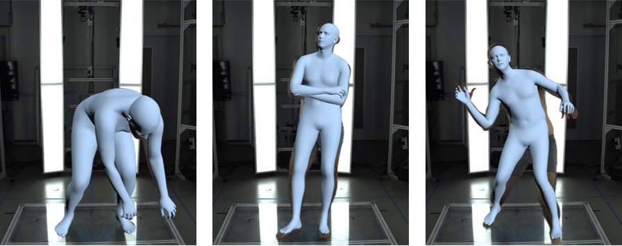
(a) EHF dataset

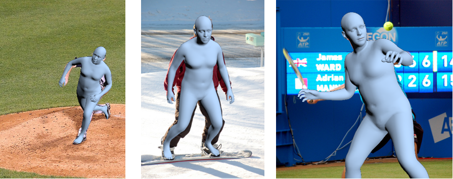
(b) MSCOCO dataset

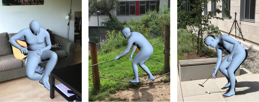
(c) 3DPW dataset

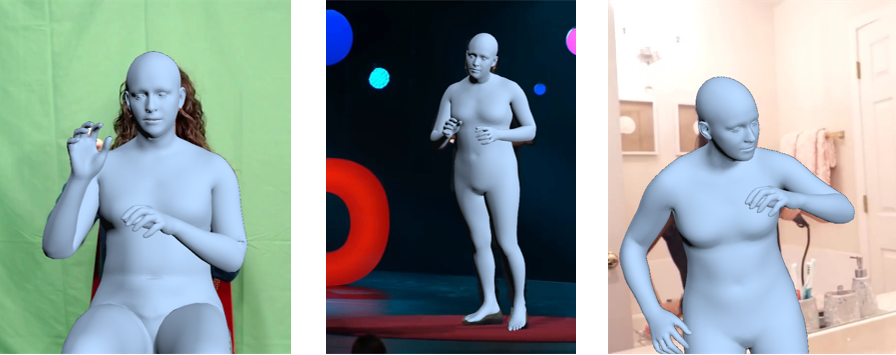
(d) UBody dataset

Figure 5: Qualitative evaluations of HMR leveraging DPoser as pose prior. CLIFF [51] serves as the optimization initializer.

We probe the efficacy of DPoser in HMR, focusing on estimating human pose and shape from monocular images. We conduct experiments on the EHF dataset [35] and benchmark our method against existing SOTA priors. Our optimization-based framework incorporates two initialization paradigms: (1) a baseline initialization that utilizes mean pose values and a default camera setup, and (2) an advanced initialization scheme that leverages CLIFF [51], a pre-trained regression-based model tailored for HMR.

As shown in Tab. 2, DPoser demonstrates robust performance in HMR. With baseline initialization, it closely rivals the strong constraints of the GMM prior [34]. When enhanced by advanced initialization via CLIFF, DPoser surpasses established deep priors like Pose-NDF [36]. Fig. 5 visually confirms DPoser’s superior efficacy and adaptability across multiple datasets including EHF [35], MSCOCO [54], 3DPW [55], and UBody [53]. Further qualitative comparisons are available in the Appendix.

Methods	AMASS [52]	HPS [56]
VPoser [35]	23.42	22.78
Pose-NDF [36]	22.13	23.82
MVAE [40]	26.80	N/A
HuMoR [39]	22.69	N/A
DPoser (ours)	19.87	20.54

Table 4: Performance metrics (MPJPE) for motion denoising.

5.4 Pose Completion

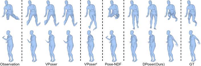
Figure 6: Qualitative evaluations of pose completion. Three hypotheses are drawn from VPoser [35] and our DPoser.

Timestep scheduling	HMR		Pose Completion		Motion Denoising
	PA-MPJPE $\downarrow$	MPJPE $\downarrow$	MPVPE $\downarrow$	MPJPE $\downarrow$	MPVPE $\downarrow$	MPJPE $\downarrow$
Random	68.21	98.57	109.53	102.37	43.33	23.87
Fixed	57.72	85.11	40.44	36.70	45.69	22.54
Full annealed	61.15	85.27	42.97	39.42	39.72	20.80
Truncated annealed	57.28	84.79	39.77	36.15	38.21	19.87

Table 5: Comparative performance of different timestep scheduling across pose-related tasks.

Noise std	AMASS [52]	HPS [56]
20.00	31.93/13.64	31.93/13.45
40.00	63.81/19.87	63.81/20.54
100.00	159.78/33.18	159.78/35.32

Table 6: DPoser in motion denoising under varying noise scales. MPJPE is reported as before/after applying DPoser denoising.

In practical scenarios like those encountered in the UBody dataset [53] (refer to Fig. 5(d)), HMR algorithms often grapple with occlusions leading to incomplete 3D pose estimates. In this context, our ambition is to recover full 3D poses from such partially observed data, where the unseen parts are initialized with random noise.

Given that Pose-NDF [36] and VPoser [35] have not been previously scrutinized for this task, we introduce two experimental paradigms—generation-based and optimization-based. In the optimization regimen, we incorporate an L2-norm fidelity term for the observed pose and constrain the entire pose using these deep priors. In contrast, the generation-based scheme for VPoser involves encoding the whole pose, followed by decoding and sampling from the resulting Gaussian distributions. For Pose-NDF, we iteratively project the whole pose onto the learned manifold, replacing the unmasked components with known data. For DPoser, we report optimization-based outcomes while the generation-based results employing other inverse problem solvers [8, 20, 19] can be checked in the Appendix.

Given the task’s inherent ambiguity, we sample multiple solutions and select the best-fitting one, except the deterministic Pose-NDF. Tab. 3 and Fig. 6 demonstrate DPoser’s superiority in pose completion under occlusions, offering multiple plausible solutions, unlike VPoser [35] and Pose-NDF [36], with the latter facing generalization issues when applied to such unseen noisy poses.

5.5 Motion Denoising

Though not initially designed for temporal tasks, DPoser shows remarkable proficiency in motion denoising. The task aims to estimate clean body poses from noisy 3D joint positions in motion capture sequences. Adhering to the setup outlined in HuMoR [39], we utilize 60-frame sequences from the AMASS [52] test dataset and artificially introduce Gaussian noise with a standard deviation of 40 mm to the 3D joint positions. Moreover, we conduct experiments on HPS datasets [56] without additional training to validate the generalization. Our optimization loss is composed of a data fidelity term, a temporal consistency term, and our pose prior, as discussed in the Appendix.

As presented in Tab. 4, DPoser sets a new standard in motion denoising, outperforming even specialized motion priors like HuMoR [39]. To further confirm the robustness of DPoser, we conduct evaluations under varying conditions to gauge DPoser’s denoising capabilities. The results, detailed in Tab. 6, reveal that DPoser consistently achieves significant reductions in MPJPE, maintaining robust performance even under extreme noise conditions, specifically at a noise standard deviation of 100.00 mm. We direct the reader to our Appendix for qualitative assessments.

5.6 Ablation Study

In our ablation study, we initially focus on the impact of truncated timestep scheduling on DPoser’s performance. This involves contrasting our proposed scheduling strategy against three established methods—random, fixed, and full annealed scheduling [62, 18, 19, 8]. As Tab. 5 demonstrates, our strategy consistently outperforms these alternatives across all evaluated tasks. Further, we delve into the training aspects of DPoser, such as rotation representations and the integration of an auxiliary loss akin to HuMoR [39]. Additionally, using the same trained prior, we benchmark DPoser against SOTA diffusion-based inverse problem solvers [8, 20, 19] on the pose completion task. The results underscore that DPoser not only proves versatile across multiple pose-related tasks but also excels in performance. Detailed findings and analyses from these ablation studies are presented in the Appendix.

6 Conclusion

We introduce DPoser, a robust and vetsatile human pose prior framework grounded in diffusion models. Engineered for flexibility, DPoser shines across multiple pose-related tasks, enhanced by our innovative truncated timestep scheduling for test-time optimization. Comprehensive experiments substantiate DPoser’s superior performance over existing state-of-the-art pose priors, establishing it as an effective solution for a wide range of applications.

Limitation and future work. While our framework benefits from variational diffusion sampling [18], it also shares its limitations, such as the mode-seeking behavior. Future research could look into enhancing solution diversity via techniques like particle-based variational inference [30, 31]. Furthermore, within the broader context of inverse problems, a plethora of existing methods [22, 23, 25, 24] could be adapted to leverage our diffusion-based prior. Exploring these methods holds great potential for future progress.

Supplementary Material:
DPoser: Diffusion Model as Robust 3D Human Pose Prior

A Parameterization of Score-based Diffusion Models

In the seminal work by Song et al. [8], it is demonstrated that both score-based generative models [6] and diffusion probabilistic models [10] can be understood as discretized versions of stochastic differential equations (SDEs) defined by score functions. This unification allows the training objective to be interpreted either as learning a time-dependent denoiser or as learning a sequence of score functions that describe increasingly noisy versions of the data.

We begin by revisiting the training objective for score-based models [6] to elucidate the link with diffusion models [10]. Consider the transition kernel of the forward diffusion process $p_{0t}(\mathbf{x}_{t}|\mathbf{x}_{0})=\mathcal{N}(\mathbf{x}_{t};\alpha_{t}\mathbf{x}_{0},\sigma_{t}^{2}\mathbf{I})$. Our goal is to learn score functions $\nabla_{\mathbf{x}_{t}}\log p_{t}(\mathbf{x}_{t})$ through a neural network $s_{\theta}(\mathbf{x}_{t};t)$, by minimizing the L2 loss as follows (we omit the expectation operator for conciseness) :

$$\mathbb{E}\left[w(t)||s_{\theta}(\mathbf{x}_{t};t)-\nabla_{\mathbf{x}_{t}}\log p_{t}\left(\mathbf{x}_{t}\right)||_{2}^{2}\right].$$ (14)

Here, $\mathbf{x}_{t}=\alpha_{t}\mathbf{x}_{0}+\sigma_{t}\epsilon$, where $\epsilon\sim\mathcal{N}(\mathbf{0},\mathbf{I})$.

Based on denoising score matching [2], we know the minimizing objective Eq. (14) is equivalent to the following tractable term:

$$\mathbb{E}\left[w(t)||s_{\theta}(\mathbf{x}_{t};t)-\nabla_{\mathbf{x}_{t}}\log p_{0t}(\mathbf{x}_{t}|\mathbf{x}_{0})||_{2}^{2}\right].$$ (15)

To link this with the noise predictor $\epsilon_{\theta}(\mathbf{x}_{t};t)$ in diffusion models, we can employ the reparameterization $s_{\theta}(\mathbf{x}_{t};t)=-\frac{\epsilon_{\theta}(\mathbf{x}_{t};t)}{\sigma_{t}}$. Then, Eq. (15) can be simplified as follows:

$$w(t)||-\frac{\epsilon_{\theta}(\mathbf{x}_{t};t)}{\sigma_{t}}-\nabla_{\mathbf{x}_{t}}\log p_{0t}(\mathbf{x}_{t}\mid\mathbf{x}_{0})||_{2}^{2}$$

$$= w(t)||-\frac{\epsilon_{\theta}(\mathbf{x}_{t};t)}{\sigma_{t}}+\frac{(\mathbf{x}_{t}-\alpha_{t}\mathbf{x}_{0})}{\sigma_{t}^{2}}||_{2}^{2}$$

$$= w(t)||-\frac{\epsilon_{\theta}(\mathbf{x}_{t};t)}{\sigma_{t}}+\frac{\sigma_{t}\epsilon}{\sigma_{t}^{2}})||_{2}^{2}$$

$$= \frac{w(t)}{\sigma_{t}^{2}}||\epsilon_{\theta}(\mathbf{x}_{t};t)-\epsilon)||_{2}^{2}$$ (16)

The resulting form of Eq. (16) aligns precisely with the noise prediction form of diffusion models [10] (refer to Eq. (4)). This implies that by training $\epsilon_{\theta}(\mathbf{x}_{t};t)$ in a diffusion model context, we simultaneously get a handle on the score function, approximated as $\nabla_{\mathbf{x}_{t}}\log p_{t}(\mathbf{x}_{t})\approx-\frac{\epsilon_{\theta}(\mathbf{x}_{t};t)}{\sigma_{t}}$.

B View DPoser as Score Distillation Sampling

Strategy	HMR		Pose Completion		Motion Denoising
	PA-MPJPE $\downarrow$	MPJPE $\downarrow$	MPVPE $\downarrow$	MPJPE $\downarrow$	MPVPE $\downarrow$	MPJPE $\downarrow$
1step	57.28	84.79	39.77	36.15	38.21	19.87
5steps	57.61	85.14	41.30	37.58	40.22	21.21
10steps	57.66	85.07	41.28	37.39	40.69	21.34

Table S-1: Efficacy of different denoising steps in DPoser’s optimization.

Interestingly, the gradient of DPoser in Eq. (10) coincides with Score Distillation Sampling (SDS) [27, 28], which can be interpreted as aiming to minimize the following KL divergence:

$$KL\big{(}p_{0t}\left(\mathbf{x}_{t}\mid\mathbf{x}_{0}\right)\parallel p_{t}^{\mathtt{SDE}}\left(\mathbf{x}_{t};\theta\right)\big{)},$$ (17)

where $p_{t}^{\mathtt{SDE}}\left(\mathbf{x}_{t};\theta\right)$ denote the marginal distribution whose score function is estimated by $\epsilon_{\theta}(\mathbf{x}_{t};t)$. For the specific case where $t\to 0$, this term encourages the Dirac distribution $\delta(\mathbf{x}_{0})$ (i.e., the optimized variable) to gravitate toward the learned data distribution $p_{0}^{\mathtt{SDE}}\left(\mathbf{x}_{0};\theta\right)$, while the Gaussian perturbation like Eq. (17) softens the constraint. Building on this understanding, we can borrow advanced techniques from SDS [27, 28]—a rapidly evolving area ripe for methodological innovations [31, 32, 29]. To extend this, we experiment with a multi-step denoising strategy adapted from HiFA [29], substituting our original one-step denoising process. This alternative, however, yields suboptimal results across all evaluation metrics, as demonstrated in Tab. S-1. A plausible explanation could be that our proposed truncated timestep scheduling effectively manages low noise levels (i.e., small $t$), thus negating the need for more denoising steps.

C Experimental Details

This section elaborates on the specifics of our pose completion and motion denoising experiments, and also highlights DPoser’s proficiency in pose interpolation tasks.

C.1 Pose completion

For partial observations $\mathbf{y}$, the measurement operator $\mathcal{A}$ is modeled as a mask matrix $M\in\mathbb{R}^{d\times n}$. Based on our optimization framework (i.e., Algorithm 1), we define the task-specific loss, $L_{\text{comp}}$, as follows:

$$L_{\text{comp}}=||M\mathbf{x}_{0}-\mathbf{y}||_{2}^{2}.$$ (18)

Here, $\mathbf{x}_{0}$ denotes the whole body pose $\theta$ we try to recover, where the unseen parts are initialized as random noise. In ourthe following ablated studies, if not specified, the evaluation is performed using 10 hypotheses on the AMASS [52] test set with left leg occlusion.

C.2 Motion denoising

Methods	AMASS [52]		HPS [56]
	20mm	100mm	20mm	100mm
VPoser [35]	15.20	49.10	17.24	46.69
Pose-NDF [36]	13.84	46.10	15.62	47.50
DPoser (ours)	13.64	33.18	13.45	35.32

Table S-2: Performance comparison of motion denoising under varying noise scales. MPJPE is reported afters denoising.

Adhering to Pose-NDF settings [36], we aim to refine noisy joint positions $J_{\text{obs}}^{t}$ over $N$ frames to obtain clean poses $\theta^{t}$, initialized from mean poses in SMPL with small noise. We formulate the task-specific loss combining an observation fidelity term $L_{\text{obs}}$ and a temporal consistency term $L_{\text{temp}}$:

$$L_{\text{obs}} =\sum_{t=0}^{N-1}||M_{J}(\theta^{t},\beta_{0})-J_{\text{obs}}^{t}||_{2}^{2},$$ (19)

$$L_{\text{temp}} =\sum_{t=1}^{N-1}||M_{J}(\theta^{t-1},\beta_{0})-M_{J}(\theta^{t},\beta_{0})||_{2}^{2},$$ (20)

where $M_{J}$ denotes the 3D joint positions regressed from SMPL [33] and $\beta_{0}$ is the constant mean shape parameters.

In complement to the comparative analysis presented in Tab. 4, we extend our evaluation to include scenarios with varying noise levels. This extended examination, detailed in Tab. S-2, showcases DPoser’s exceptional performance against state-of-the-art (SOTA) pose priors, especially under conditions of high noise, manifesting DPoser’s resilience to noise.

C.3 Pose interpolation

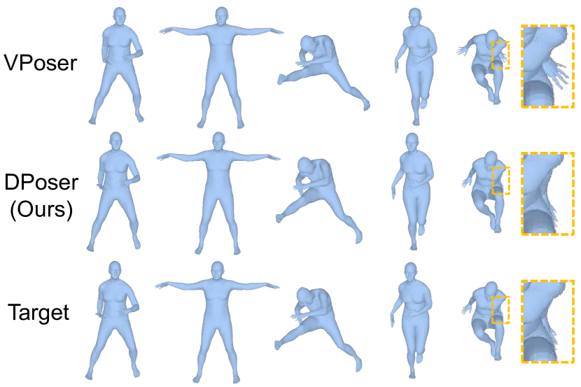
(a) Pose reconstruction.

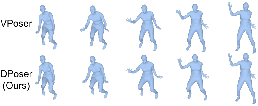
(b) Interpolation between two poses.

Figure S-1: Visual results of pose reconstruction and interpolation.

For the forward SDE (Eq. (1)), there exists a probability flow ODE with the same marginal probability densities corresponding to it, expressed as: [8]

$$\mathrm{d}\mathbf{x}=[\mu(t)\mathbf{x}-\frac{1}{2}g(t)^{2}\nabla_{\mathbf{x}_{t}}\log p_{t}\left(\mathbf{x}_{t}\right)]\mathrm{d}t.$$ (21)

By replacing $\nabla_{\mathbf{x}_{t}}\log p_{t}(\mathbf{x}_{t})$ with our approximation $-\frac{\epsilon_{\theta}(\mathbf{x}_{t};t)}{\sigma_{t}}$, this ODE can be treated as a neural ODE [5], which is fully invertible. By integrating through it, we can encode any data point $\mathbf{x}_{0}$ into its latent representation $\bar{\mathbf{x}}_{1}$ and decode it through its reverse-time counterpart.

For interpolation, we start with two poses, $\mathbf{x}_{0}^{0}$ and $\mathbf{x}_{0}^{1}$, and encode them into latent representations $\bar{\mathbf{x}}_{1}^{0}$ and $\bar{\mathbf{x}}_{1}^{1}$. Utilizing spherical linear interpolation (Slerp), we obtain interpolated latents $\bar{\mathbf{x}}_{1}^{t}=\text{Slerp}(\bar{\mathbf{x}}_{1}^{0},\bar{\mathbf{x}}_{1}^{1};t)$ for $t\in[0,1]$, which are then decoded to produce novel poses. The Slerp function is defined as:

$$\text{Slerp}(A,B;t)=\frac{\sin((1-t)\omega)}{\sin\omega}A+\frac{\sin(t\omega)}{\sin\omega}B,$$ (22)

where $\omega=\arccos(A\cdot B/\|A\|\|B\|)$.

To validate the informativeness of our encoding, we employ MPJPE and MPVPE metrics for reconstruction evaluation. Compared to VPoser [35], a VAE-based prior, DPoser exhibits superior performance with 4.79mm and 6.58mm errors, against 9.85mm and 12.16mm, respectively. Qualitative results further confirm DPoser’s strong reconstruction and smooth interpolation capabilities, as shown in Fig. S-1.

D Ablated DPoser Training

Normalization	HMR		Pose Completion		Motion Denoising
	PA-MPJPE $\downarrow$	MPJPE $\downarrow$	MPVPE $\downarrow$	MPJPE $\downarrow$	MPVPE $\downarrow$	MPJPE $\downarrow$
w/o norm	58.62	83.75	60.70	55.47	44.82	24.04
min-max	59.55	85.63	58.18	53.06	42.70	21.29
z-score	57.66	85.47	52.86	48.27	38.57	20.24

Table S-3: Evaluation of DPoser’s performance under different normalization methods, specifically for the axis-angle rotation representation.

Representation	HMR		Pose Completion		Motion Denoising
	PA-MPJPE $\downarrow$	MPJPE $\downarrow$	MPVPE $\downarrow$	MPJPE $\downarrow$	MPVPE $\downarrow$	MPJPE $\downarrow$
axis-angle	57.28	84.79	52.14	47.60	38.21	19.87
6D rotations	58.02	85.93	56.28	51.54	38.44	20.12

Table S-4: Comparative performance of rotation representations under z-score normalization across multiple tasks and metrics.

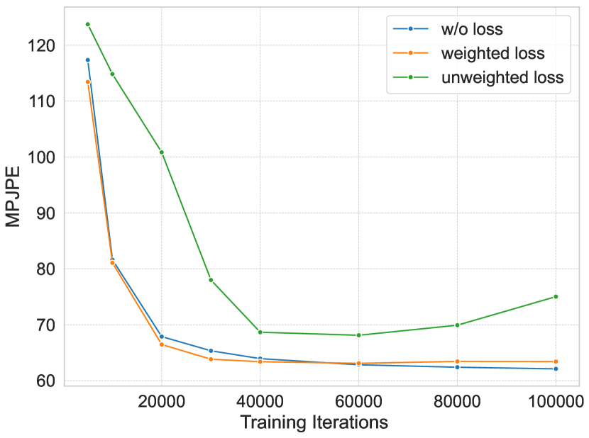
Figure S-2: Evolution of MPJPE during DPoser training, evaluated on pose completion. The evaluation is conducted on the AMASS [52] test set, utilizing 10 hypotheses and simulating occlusion scenarios affecting both legs.

Building on the insights shared in Sec. 4.1 in our main text, this part dissects the impact of different rotation representations and normalization techniques on DPoser’s performance. Initially, we examine axis-angle representation, comparing various normalization strategies: min-max scaling, z-score normalization, and no normalization. Our findings, summarized in Tab. S-3, indicate that z-score normalization is generally the most effective. Subsequently, using this optimal normalization, we explore 6D rotations [59] as an alternative. As evidenced by Tab. S-4, axis-angle representation offers superior performance. This preference can be attributed to the effective modeling capabilities of diffusion models, along with the inherent advantages of axis-angle in capturing bounded joint rotations.

Inspired by HuMoR [39], we experiment with integrating the SMPL body model [33] as a regularization term during DPoser’s training. Alongside the prediction of additive noise, as outlined in Eq (4), we employ a 10-step DDIM sampler [11] to recover a “clean” version of the pose, denoted as $\tilde{\mathbf{x}}_{0}$, from the diffused $\mathbf{x}_{t}$. The regularization loss aims to minimize the discrepancy between the original and recovered poses under the SMPL body model $M$:

$$L_{\mathrm{reg}}= ||M_{J}(\tilde{\mathbf{x}}_{0},\beta_{0})-M_{J}(\mathbf{x}_{0},\beta_{0})||_{2}^{2}$$

$$+||M_{V}(\tilde{\mathbf{x}}_{0},\beta_{0})-M_{V}(\mathbf{x}_{0},\beta_{0})||_{2}^{2}.$$

Here, $\beta_{0}$ represents the mean shape parameters in SMPL. To account for denoising errors, we scale the regularization loss by $\mathrm{log}(1+\frac{\alpha_{t}}{\sigma_{t}})$, thereby increasing the weight for samples with smaller $t$ values (less noise). Fig. S-2 visualizes the impact of this regularization on MPJPE during the training, specifically for pose completion tasks with occlusion of both legs. We observe that weighted regularization offers slight performance gains in the early training process, while the absence of weighting introduces instability and deterioration in results. Despite these insights, the computational cost of incorporating the SMPL model—especially for our large batch size of 1280—makes the training approximately 8 times slower. Therefore, we opted not to include this regularization in our main experiments.

E Extended DPoser Optimization

Methods	Occ. left leg		Occ. legs		Occ. arms		Occ. trunk
	MPVPE $\downarrow$	MPJPE $\downarrow$	MPVPE $\downarrow$	MPJPE $\downarrow$	MPVPE $\downarrow$	MPJPE $\downarrow$	MPVPE $\downarrow$	MPJPE $\downarrow$
ScoreSDE [8]	52.86	48.27	80.68	74.74	82.38	65.81	27.97	17.27
DPS [19]	41.99	38.08	66.16	61.28	64.75	51.75	25.68	15.90
MCG [20]	51.97	47.46	80.07	74.14	82.22	65.58	27.93	17.27
DPoser (ours)	39.77	36.15	65.24	60.54	66.77	52.75	21.58	13.41

Table S-5: Comparative evaluation of diffusion-based solvers for pose completion.

In addressing pose-centric tasks as inverse problems, we propose a versatile optimization framework, which employs variational diffusion sampling as its foundational approach [18]. Our exploration extends to an array of diffusion-based methodologies for solving these complex inverse problems. Among the techniques considered are ScoreSDE [8], MCG [20], and DPS [19]. These methods augment standard generative processes with observational data, either by employing gradient-based guidance or back-projection techniques. We compare these methods with our DPoser for pose completion tasks. Our findings, captured in Tab. S-5, reveal that DPoser outperforms the competitors under most occlusion conditions. Consequently, DPoser emerges not merely as a universally applicable solution to pose-related tasks, but also as an exceptionally efficient one.

It is worth mentioning that methods rooted in generative frameworks [8, 20, 19, 21] can pose challenges for broader applicability in pose-centric tasks. For instance, in blind inverse problems—certain parameters in $\mathcal{A}$ (e.g., camera models in HMR) are unknown—generative methods are less straightforward to implement. ZeDO [44], a recent study focusing on the 2D-3D lifting task, adopts the ScoreSDE [8] framework and refines camera translations by solving an optimization sub-problem after each generative step. However, directly porting this strategy to HMR is non-trivial, owing to the added complexity of body shape parameter optimization—a feature currently absent in our DPoser model. Although some state-of-the-art techniques [25, 24] offer solutions by jointly modeling operator $\mathcal{A}$ and data distributions, a full-fledged discussion on this subject is beyond this paper’s purview and remains an open question for future work.

F More Qualitative Results

We show more qualitative results for pose generation (Fig. S-3), pose completion (Fig. S-4), human mesh recovery (Fig. S-5), and motion denoising (Fig. S-6).

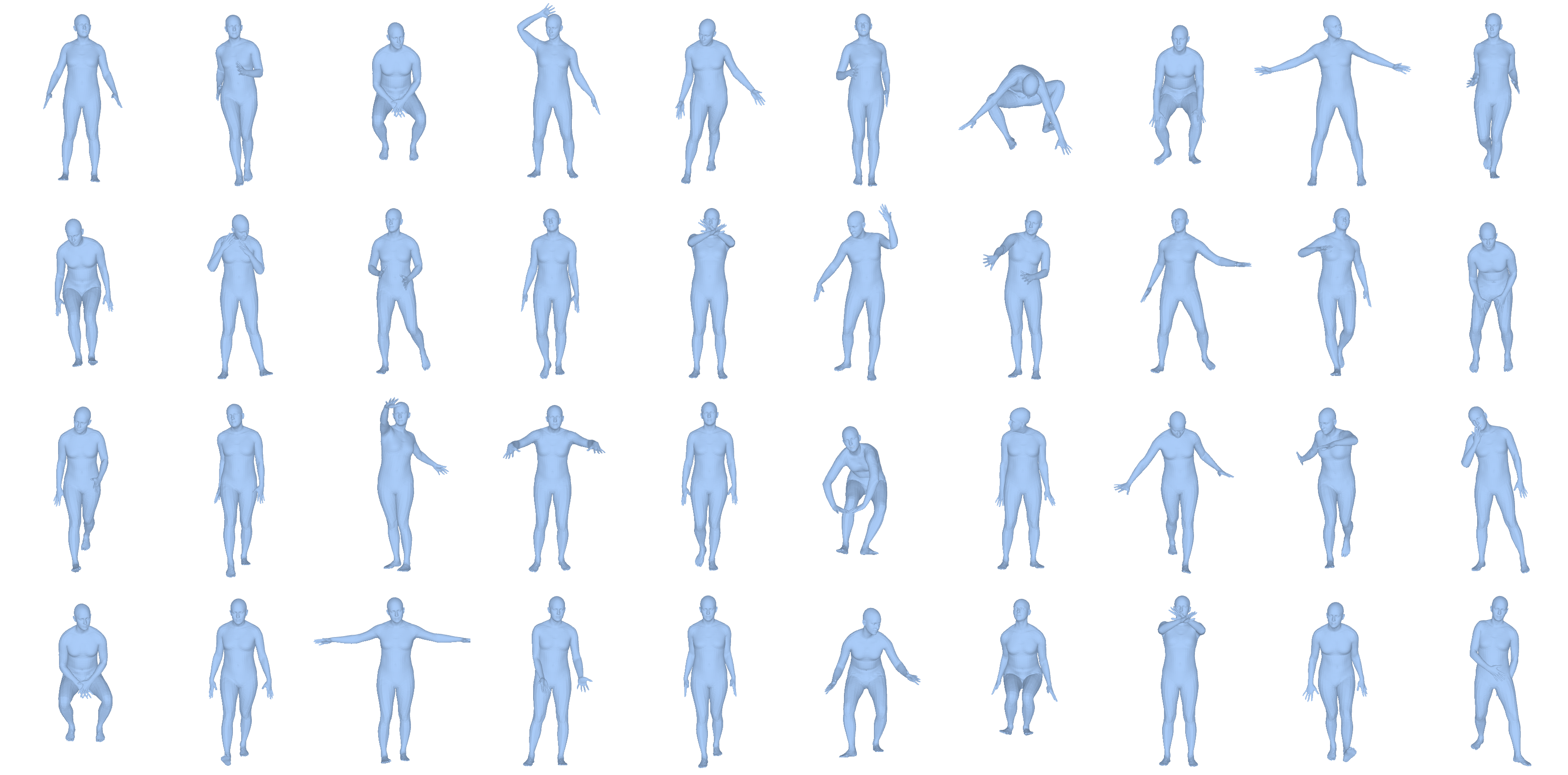
Figure S-3: Pose generation. DPoser can generate diverse and realistic poses.

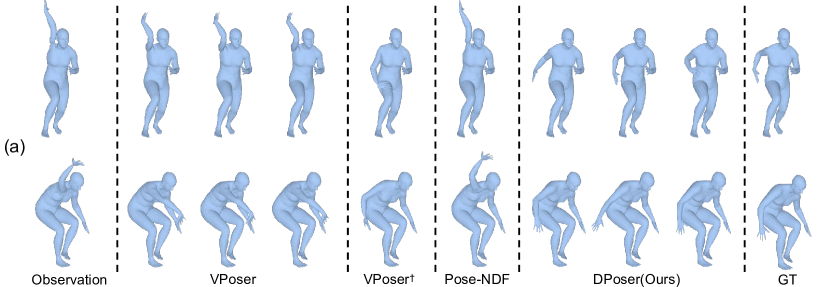
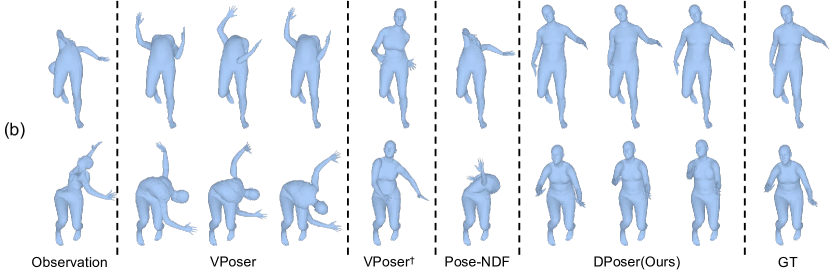
Figure S-4: Pose completion. (a) Right arm under occlusion. (b) Trunk under occlusion.

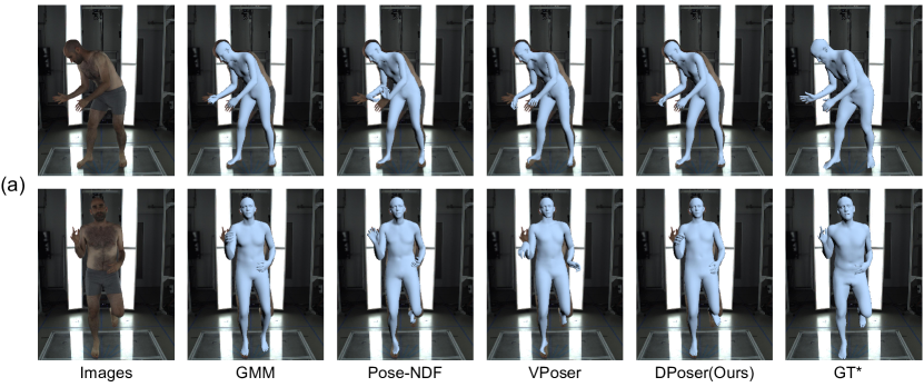
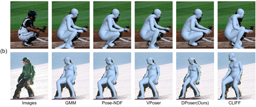
Figure S-5: Human mesh recovery. (a) Initialization using mean poses and default camera. *Ground truth for the EHF dataset is annotated in SMPL-X [35], which extends SMPL [33] with fully articulated hands and an expressive face. (b) Initialization using the CLIFF [51] prediction.

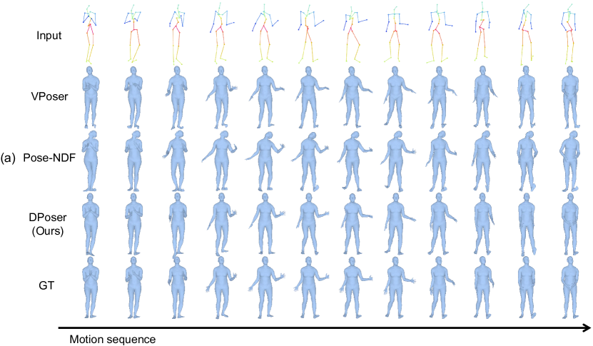
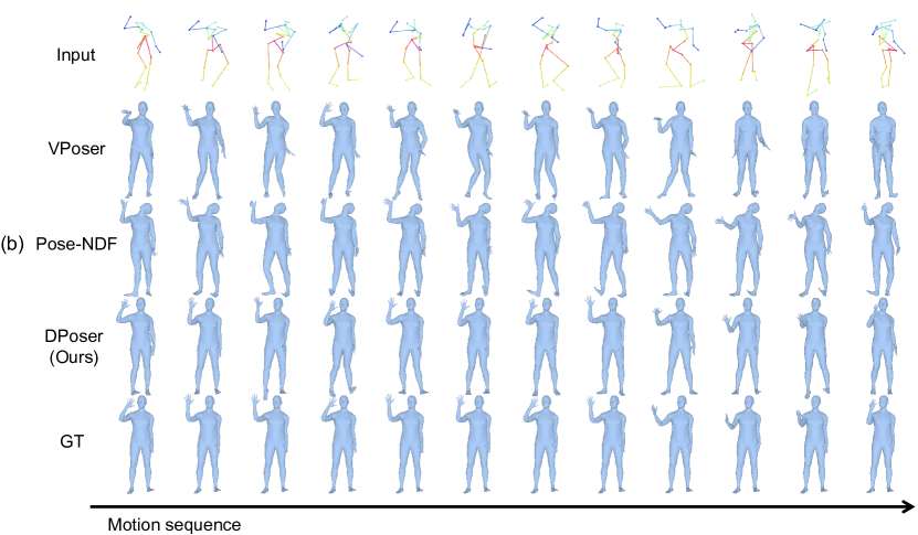
Figure S-6: Motion denoising. (a) Gaussian noise with 40mm standard deviation. (b) Gaussian noise with 100mm standard deviation. We visualize every 20^th of the sequence.

References

- [1] B. Efron, “Tweedie’s formula and selection bias,” Journal of the American Statistical Association, 2011.
- [2] P. Vincent, “A connection between score matching and denoising autoencoders,” Neural computation, 2011.
- [3] J. Sohl-Dickstein, E. Weiss, N. Maheswaranathan, and S. Ganguli, “Deep unsupervised learning using nonequilibrium thermodynamics,” in ICML, 2015.
- [4] Q. Liu, J. Lee, and M. Jordan, “A kernelized stein discrepancy for goodness-of-fit tests,” in ICML, 2016.
- [5] R. T. Chen, Y. Rubanova, J. Bettencourt, and D. K. Duvenaud, “Neural ordinary differential equations,” NeurIPS, 2018.
- [6] Y. Song and S. Ermon, “Generative modeling by estimating gradients of the data distribution,” NeurIPS, 2019.
- [7] S. Särkkä and A. Solin, Applied stochastic differential equations. Cambridge University Press, 2019, vol. 10.
- [8] Y. Song, J. Sohl-Dickstein, D. P. Kingma, A. Kumar, S. Ermon, and B. Poole, “Score-based generative modeling through stochastic differential equations,” arXiv preprint arXiv:2011.13456, 2020.
- [9] Y. Song, C. Durkan, I. Murray, and S. Ermon, “Maximum likelihood training of score-based diffusion models,” NeurIPS, 2021.
- [10] J. Ho, A. Jain, and P. Abbeel, “Denoising diffusion probabilistic models,” NeurIPS, 2020.
- [11] J. Song, C. Meng, and S. Ermon, “Denoising diffusion implicit models,” arXiv preprint arXiv:2010.02502, 2020.
- [12] P. Dhariwal and A. Nichol, “Diffusion models beat gans on image synthesis,” NeurIPS, 2021.
- [13] R. Rombach, A. Blattmann, D. Lorenz, P. Esser, and B. Ommer, “High-resolution image synthesis with latent diffusion models,” in CVPR, 2022.
- [14] T. Karras, M. Aittala, T. Aila, and S. Laine, “Elucidating the design space of diffusion-based generative models,” NeurIPS, 2022.
- [15] J. Choi, J. Lee, C. Shin, S. Kim, H. Kim, and S. Yoon, “Perception prioritized training of diffusion models,” in CVPR, 2022.
- [16] D. P. Kingma and M. Welling, “Auto-encoding variational bayes,” arXiv preprint arXiv:1312.6114, 2013.
- [17] I. Goodfellow, J. Pouget-Abadie, M. Mirza, B. Xu, D. Warde-Farley, S. Ozair, A. Courville, and Y. Bengio, “Generative adversarial networks,” Communications of the ACM, 2020.
- [18] M. Mardani, J. Song, J. Kautz, and A. Vahdat, “A variational perspective on solving inverse problems with diffusion models,” arXiv preprint arXiv:2305.04391, 2023.
- [19] H. Chung, J. Kim, M. T. Mccann, M. L. Klasky, and J. C. Ye, “Diffusion posterior sampling for general noisy inverse problems,” arXiv preprint arXiv:2209.14687, 2022.
- [20] H. Chung, B. Sim, D. Ryu, and J. C. Ye, “Improving diffusion models for inverse problems using manifold constraints,” NeurIPS, 2022.
- [21] B. Kawar, M. Elad, S. Ermon, and J. Song, “Denoising diffusion restoration models,” NeurIPS, 2022.
- [22] J. Song, A. Vahdat, M. Mardani, and J. Kautz, “Pseudoinverse-guided diffusion models for inverse problems,” in ICLR, 2022.
- [23] B. Boys, M. Girolami, J. Pidstrigach, S. Reich, A. Mosca, and O. D. Akyildiz, “Tweedie moment projected diffusions for inverse problems,” arXiv preprint arXiv:2310.06721, 2023.
- [24] N. Murata, K. Saito, C.-H. Lai, Y. Takida, T. Uesaka, Y. Mitsufuji, and S. Ermon, “Gibbsddrm: A partially collapsed gibbs sampler for solving blind inverse problems with denoising diffusion restoration,” arXiv preprint arXiv:2301.12686, 2023.
- [25] H. Chung, J. Kim, S. Kim, and J. C. Ye, “Parallel diffusion models of operator and image for blind inverse problems,” in CVPR, 2023.
- [26] A. Graikos, N. Malkin, N. Jojic, and D. Samaras, “Diffusion models as plug-and-play priors,” NeurIPS, 2022.
- [27] B. Poole, A. Jain, J. T. Barron, and B. Mildenhall, “Dreamfusion: Text-to-3d using 2d diffusion,” arXiv preprint arXiv:2209.14988, 2022.
- [28] H. Wang, X. Du, J. Li, R. A. Yeh, and G. Shakhnarovich, “Score jacobian chaining: Lifting pretrained 2d diffusion models for 3d generation,” in CVPR, 2023.
- [29] J. Zhu and P. Zhuang, “Hifa: High-fidelity text-to-3d with advanced diffusion guidance,” arXiv preprint arXiv:2305.18766, 2023.
- [30] Q. Liu and D. Wang, “Stein variational gradient descent: A general purpose bayesian inference algorithm,” NeurIPS, 2016.
- [31] Z. Wang, C. Lu, Y. Wang, F. Bao, C. Li, H. Su, and J. Zhu, “Prolificdreamer: High-fidelity and diverse text-to-3d generation with variational score distillation,” arXiv preprint arXiv:2305.16213, 2023.
- [32] J. Wu, X. Gao, X. Liu, Z. Shen, C. Zhao, H. Feng, J. Liu, and E. Ding, “Hd-fusion: Detailed text-to-3d generation leveraging multiple noise estimation,” arXiv preprint arXiv:2307.16183, 2023.
- [33] M. Loper, N. Mahmood, J. Romero, G. Pons-Moll, and M. J. Black, “Smpl: A skinned multi-person linear model,” in Seminal Graphics Papers: Pushing the Boundaries, Volume 2, 2023.
- [34] F. Bogo, A. Kanazawa, C. Lassner, P. Gehler, J. Romero, and M. J. Black, “Keep it smpl: Automatic estimation of 3d human pose and shape from a single image,” in ECCV, 2016.
- [35] G. Pavlakos, V. Choutas, N. Ghorbani, T. Bolkart, A. A. Osman, D. Tzionas, and M. J. Black, “Expressive body capture: 3d hands, face, and body from a single image,” in CVPR, 2019.
- [36] G. Tiwari, D. Antić, J. E. Lenssen, N. Sarafianos, T. Tung, and G. Pons-Moll, “Pose-ndf: Modeling human pose manifolds with neural distance fields,” in ECCV, 2022.
- [37] S. Aliakbarian, F. S. Saleh, M. Salzmann, L. Petersson, and S. Gould, “A stochastic conditioning scheme for diverse human motion prediction,” in CVPR, 2020.
- [38] A. Davydov, A. Remizova, V. Constantin, S. Honari, M. Salzmann, and P. Fua, “Adversarial parametric pose prior,” in CVPR, 2022.
- [39] D. Rempe, T. Birdal, A. Hertzmann, J. Yang, S. Sridhar, and L. J. Guibas, “Humor: 3d human motion model for robust pose estimation,” in ICCV, 2021.
- [40] H. Y. Ling, F. Zinno, G. Cheng, and M. Van De Panne, “Character controllers using motion vaes,” TOG, 2020.
- [41] K. Holmquist and B. Wandt, “Diffpose: Multi-hypothesis human pose estimation using diffusion models,” in ICCV, 2023.
- [42] Z. Qiu, Q. Yang, J. Wang, X. Wang, C. Xu, D. Fu, K. Yao, J. Han, E. Ding, and J. Wang, “Learning structure-guided diffusion model for 2d human pose estimation,” arXiv preprint arXiv:2306.17074, 2023.
- [43] H. Ci, M. Wu, W. Zhu, X. Ma, H. Dong, F. Zhong, and Y. Wang, “Gfpose: Learning 3d human pose prior with gradient fields,” in CVPR, 2023.
- [44] Z. Jiang, Z. Zhou, L. Li, W. Chai, C.-Y. Yang, and J.-N. Hwang, “Back to optimization: Diffusion-based zero-shot 3d human pose estimation,” arXiv preprint arXiv:2307.03833, 2023.
- [45] M. Zhao, M. Liu, B. Ren, S. Dai, and N. Sebe, “Modiff: Action-conditioned 3d motion generation with denoising diffusion probabilistic models,” arXiv preprint arXiv:2301.03949, 2023.
- [46] Y. Shafir, G. Tevet, R. Kapon, and A. H. Bermano, “Human motion diffusion as a generative prior,” arXiv preprint arXiv:2303.01418, 2023.
- [47] L. Li, L. Zhuo, B. Zhang, L. Bo, and C. Chen, “Diffhand: End-to-end hand mesh reconstruction via diffusion models,” arXiv preprint arXiv:2305.13705, 2023.
- [48] H. Cho and J. Kim, “Generative approach for probabilistic human mesh recovery using diffusion models,” in ICCV, 2023.
- [49] A. Kanazawa, M. J. Black, D. W. Jacobs, and J. Malik, “End-to-end recovery of human shape and pose,” in CVPR, 2018.
- [50] G. Georgakis, R. Li, S. Karanam, T. Chen, J. Košecká, and Z. Wu, “Hierarchical kinematic human mesh recovery,” in ECCV, 2020.
- [51] Z. Li, J. Liu, Z. Zhang, S. Xu, and Y. Yan, “Cliff: Carrying location information in full frames into human pose and shape estimation,” in ECCV, 2022.
- [52] N. Mahmood, N. Ghorbani, N. F. Troje, G. Pons-Moll, and M. J. Black, “Amass: Archive of motion capture as surface shapes,” in ICCV, 2019.
- [53] J. Lin, A. Zeng, H. Wang, L. Zhang, and Y. Li, “One-stage 3d whole-body mesh recovery with component aware transformer,” in CVPR, 2023.
- [54] T.-Y. Lin, M. Maire, S. Belongie, L. Bourdev, R. Girshick, J. Hays, P. Perona, D. Ramanan, C. L. Zitnick, and P. Dollár, “Microsoft coco: common objects in context (2014),” arXiv preprint arXiv:1405.0312, 2019.
- [55] T. Von Marcard, R. Henschel, M. J. Black, B. Rosenhahn, and G. Pons-Moll, “Recovering accurate 3d human pose in the wild using imus and a moving camera,” in ECCV, 2018.
- [56] V. Guzov, A. Mir, T. Sattler, and G. Pons-Moll, “Human poseitioning system (hps): 3d human pose estimation and self-localization in large scenes from body-mounted sensors,” in CVPR, 2021.
- [57] T. N. Kipf and M. Welling, “Semi-supervised classification with graph convolutional networks,” arXiv preprint arXiv:1609.02907, 2016.
- [58] E. Nachmani, R. S. Roman, and L. Wolf, “Non gaussian denoising diffusion models,” arXiv preprint arXiv:2106.07582, 2021.
- [59] Y. Zhou, C. Barnes, J. Lu, J. Yang, and H. Li, “On the continuity of rotation representations in neural networks,” in CVPR, 2019.
- [60] Z. Cao, T. Simon, S.-E. Wei, and Y. Sheikh, “Realtime multi-person 2d pose estimation using part affinity fields,” in CVPR, 2017.
- [61] S. Geman, “Statistical methods for tomographic image restoration,” Bull. Internat. Statist. Inst., 1987.
- [62] L. Müller, V. Ye, G. Pavlakos, M. Black, and A. Kanazawa, “Generative proxemics: A prior for 3d social interaction from images,” arXiv preprint arXiv:2306.09337, 2023.