Flexible Base Station Sleeping and Resource Cooperation Enabled Green Fully-Decoupled RAN

Abstract

Base station (BS) sleeping, a promising technique to address the growing energy consumption in wireless communication networks, encounters challenges such as coverage holes and coupled uplink and downlink transmissions. As an innovative architecture designed for future-generation mobile communication networks, the fully-decoupled radio access network (FD-RAN) is anticipated to overcome these challenges by fully decoupled control-data planes and uplink-downlink transmissions. In this paper, we investigate energy-efficient uplink FD-RAN leveraging flexible BS sleeping and resource cooperation. First, we introduce a holistic energy consumption model and formulate a bi-level energy efficiency maximizing problem for FD-RAN, involved with the joint optimization of user equipment (UE) association, BS sleeping, and power control. Subsequently, through employing the Tammer decomposition method, the formulated bi-level problem is converted into two equivalent upper-level and lower-level problems. The lower-level problem encompassed with UE power control is addressed by introducing a successive lower-bound maximization-based Dinkelbach’s algorithm, and the upper-level problem for UE association and BS sleeping is solved through a modified low-complexity many-to-many swap matching algorithm, respectively. Extensive simulation results not only demonstrate the superior effectiveness of FD-RAN and our proposed algorithms but also reveal the sources of energy efficiency gains within FD-RAN.

I Introduction

The sixth-generation network is expected to meet growing wireless communication demands via denser deployments, cloud, and edge servers, integrating artificial intelligence. However, these advancements result in a significant increase in energy consumption [1]. Notably, Vodafone reports that network base station (BS) sites contribute to nearly 73% of the total energy consumption, and this trend is on the rise [2]. Thus, mitigating the growing energy demands of BSs holds great importance for the advancement of environmentally friendly and sustainable wireless communication networks. The adoption of BS sleeping mechanisms offers a potential solution to these problems by enabling underutilized BSs to enter sleep mode and offload their traffic to neighboring BSs in a cooperative manner, leading to significant energy savings. Nonetheless, the implementation of BS sleeping faces several challenges. Due to the coupling of the control and data planes, BS sleeping may result in coverage gaps arising from the lack of control coverage. Additionally, since the uplink and downlink are coupled together, BSs are only allowed to sleep when both the uplink and downlink are simultaneously vacant, which will significantly degrade the effectiveness of the current BS sleeping scheme, especially for the situation that confronts substantial asymmetry between uplink and downlink traffic [3].

Fully-decoupled radio access network (FD-RAN) [4] presents a novel and disruptive architectural design for future-generation mobile communication networks, where BSs undergo physical decoupling into control BSs (CBSs), uplink BSs (UBSs), and downlink BSs (DBSs). By leveraging the separation of control and data planes, CBSs ensure always-on and ubiquitous coverage, while UBSs and DBSs can dynamically sleep, effectively addressing the coverage hole issue caused by BS sleeping in traditional networks. The decoupling of uplink and downlink allows UBSs to enter sleep mode optimally, needing only the uplink to be vacant without requiring both uplink and downlink to be idle, and vice versa for the downlink. In addition, flexible resource cooperation in FD-RAN is anticipated to further improve energy efficiency, as demonstrated in [5]. Based on these benefits, FD-RAN is poised to address the challenges of BS sleeping in traditional networks and achieve higher energy efficiency. Nevertheless, it also poses great challenges for FD-RAN to deal with more complicated BS sleeping management solutions compared with traditional networks, e.g., the greater degrees of freedom for user association and resource scheduling in BS sleeping schemes. As a novel architecture, holistic modeling of energy consumption in FD-RAN remains uncharted, and it is of imperative importance for advancing energy efficiency investigations.

In this work, we take the energy-efficient uplink FD-RAN into investigation, focusing on the flexible UBS sleeping and resource cooperation to maximize the overall network energy efficiency. To strike a balance between accuracy and tractability in assessing energy efficiency, we initially propose a holistic energy consumption model for the FD-RAN. Subsequently, we define an energy efficiency maximization problem based on the analysis of uplink performance and a specific power model, which is formulated as a mixed-integer nonlinear programming (MINLP) problem. This problem aims at maximizing network energy efficiency while ensuring user equipment (UE) quality of service (QoS), involving the optimization of UE association, UBS sleeping, and power control. Note that the formulated problem is non-convex and bi-level, we employ the Tammer decomposition method to convert it into an equivalent upper-level and lower-level problem. The lower-level problem encompassed with UE power control is continuous but still non-convex, which is transformed into an equivalent form and addressed using the successive lower-bound maximization based Dinkelbach’s (SLMDB) algorithm [6]. For the upper-level problem involved with UE association and UBS sleeping, we introduce a modified many-to-many swap matching (TriMSM) algorithm and leverage its low-complexity realizations to deal with the difficulty of nonlinear integer programming. The fundamental contributions of this paper are summarized as follows:

• We propose a holistic power consumption model tailored for FD-RAN, providing a precise and realistic criterion for power evaluation. Additionally, we define a specific uplink power model, presenting a more tractable criterion. To our knowledge, this is the first work in this domain.

• We devise the SLMDB algorithm to address the continuous yet non-convex power control problem. The problem is transformed into a series of approximated lower-bound concave-convex fractional programming with global convergence, which is solved by the globally optimal Dinkelbach’s algorithm.

• We propose the TriMSM algorithm and leverage its low-complexity realizations to address the nonlinear integer UE association and UBS sleeping problem. Specifically, we modify the many-to-many swap matching algorithm and design three alternative low-complexity power control algorithms, capable of guaranteeing QoS while significantly diminishing the overall computational complexity.

The remainder of this paper is structured as follows: Section II reviews related literature. Section III outlines the uplink system model, while Section IV introduces a holistic energy consumption model for FD-RAN. In Section V, we formulate the energy efficiency maximization problem and propose the overall solution framework. Detailed algorithms for lower-level and upper-level problems are presented in Section VI and Section VII, respectively. Section VIII provides extensive simulation results, and Section IX concludes the paper.

II Related Works

For a precise evaluation of the energy efficiency of various technologies, constructing rational energy consumption models is imperative, and numerous studies have been conducted in this area [7, 8, 9, 10, 11, 12, 13]. Auer et al. [8] established various power models for BSs, encompassing macro, micro, pico, and femto BSs. In addition to BSs, Bashar et al. [12] considered the power consumption of UEs. Fiorani et al. [11] devised models for the radio network and optical transport network, respectively, accounting for centralized control and processing. Furthermore, power consumption in fronthauls is explored in [13]. Investigation into BS sleeping’s impact on power consumption has been conducted by Debaillie et al. [7] and Desset et al. [9]. However, these models cannot be directly applied to FD-RAN, and existing studies only focus on a part of network power consumption, lacking comprehensiveness. In formulating a trackable problem, certain existing energy models [12, 13] are relatively ideal and simple, sacrificing some accuracy. Conversely, some models, grounded in real data, are more complex [7, 9] but also more intractable. There is an urgent need for a well-balanced assessment of energy efficiency that considers both accuracy and tractability.

BS sleeping, a promising method for substantial energy savings, encounters implementation challenges, with coverage holes emerging as a significant concern during sleeping [14]. Various approaches have been proposed to tackle this challenge. Lin et al. developed a spatio-temporal traffic prediction model aimed at capturing traffic characteristics to efficiently manage arriving UE traffic in BS sleeping schemes [15]. To optimize the timing of BS sleeping, Masoudi et al. [16] utilized a digital twin model to encapsulate the dynamic system behavior and estimate risks in advance. Zhou et al. introduced a BS sleeping scheme ensuring continuous coverage by macro BSs while allowing small BSs to dynamically sleep for energy conservation [17]. Additionally, recent studies explore promising techniques like UE association, self-organizing networks, and cell zooming [18]. Nevertheless, heterogeneous deployment introduces additional deployment costs and energy consumption. Other techniques, while mitigating the adverse effects of coverage holes, fail to address the problem fundamentally. Furthermore, the coupled uplink and downlink transmission within these works hinders optimal BS sleeping.

Resource cooperation (allocation), particularly in the context of communications, plays a pivotal role in enhancing the efficiency and reliability of networks. To address the complexity of resource cooperation problems, Ma et al. [19] utilized the block coordinate descent (BCD) based algorithm to decompose the problem into sub-problems, and alternatively solve them until convergence. Within the domain of energy efficiency, problems are often formulated as fractional programming. Shen et al. [20] highlighted a specific subset of these issues, termed concave-convex fractional problems, which can be addressed effectively. For more general cases, the need for transformations or approximations depends on the specific nature of the problem under consideration. For instance, Huang et al. [21] obtained a more solvable form of the fractional problem by introducing a new auxiliary variable. Ma et al. [19] employed the Lagrange partial relaxation method to transform integer variables into continuous ones, formulating the dual problem. Subsequently, they restored the relaxed variables back to integers, effectively addressing the problem. Guo et al. [22] utilized the generalized benders decomposition method, iteratively solving the primal and master problems to handle the integer variables. Qian et al. [23] introduced a UE-BS-subchannel matching game using many-to-many matching, proven to converge towards a stable matching. Di et al. [24] treated users and sub-channels as players, formulating the sub-channel assignment problem as a swap many-to-many matching game that converges to a two-sided exchange-stable matching. However, these methods face limitations in effectively managing and directly resolving the intricate non-convex problem in FD-RAN. Moreover, existing matching algorithms lack detailed descriptions on handling QoS constraints and fall short in terms of low-complexity implementations.

III System Model

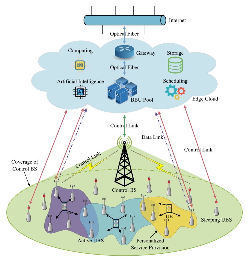
Figure 1: Energy efficient UE association and UBS sleeping in uplink FD-RAN.

III-A Network Model

We consider an uplink FD-RAN scenario depicted in Fig. 1, where a CBS is responsible for the control data plane, while $M$ UBSs handle the data plane function. Additionally, an edge cloud is deployed to provide centralized control and processing. In the control plane, we assume that $K$ single-antenna UEs and $M$ UBSs equipped with $N$ antennas are underlaid within the coverage of the CBS. Let $\mathcal{M}=\left\{1,\cdots,M\right\}$ and $\mathcal{K}=\left\{1,\cdots,K\right\}$ denote the sets of UBSs and UEs, respectively. In the data plane, multiple cooperative UBSs form UBS clusters $\mathcal{M}_{k}\subset\mathcal{M}$ for each UE $k$, enabling personalized service for each UE. Correspondingly, the UE cluster $\mathcal{K}_{m}\subset\mathcal{K}$ represents the set of UEs served by UBS $m$. After receiving data from UEs, UBSs forward the data to the edge cloud via wired backhaul. Notably, there are no active data links existing between sleeping UBSs and the edge cloud. The connections between UEs and UBSs are indicated by matrix $\mathbf{S}=\left(s_{m,k}\right)_{M\times K}$, where the binary variable $s_{m,k}=1$ indicates that UBS $m$ serves UE $k$ and vice versa. Specifically, if $\sum_{k\in\mathcal{K}}s_{m,k}=0$, it suggests that UBS $m$ is underutilized and put to sleep, denoted by $\alpha_{m}=0$, and vice versa. This information constitutes the binary UBSs operating status vector $\boldsymbol{\alpha}=\left[\alpha_{1},\cdots,\alpha_{M}\right]$ for all UBSs.

III-B Uplink Performance Analysis

III-B1 Channel Modeling and Estimation

The block fading model [25] is adopted, where the channel remains fixed within a finite-sized time-frequency coherence interval and is mutually independent across these intervals. Each coherence interval consists of $\tau_{c}$ symbols, with $\tau_{p}$ symbols dedicated to channel estimation, while the remaining $\tau_{u}=\tau_{c}-\tau_{p}$ symbols are allocated for uplink transmission. We assume that the channel response $\mathbf{h}_{m,k}$ between UE $k$ and UBS $m$ follows the correlated Rayleigh fading model:

$$\mathbf{h}_{m,k}\sim\mathcal{CN}\left(\mathbf{0}_{N},\mathbf{R}_{m,k}\right),$$ (1)

where the complex Gaussian distribution $\mathcal{CN}(\cdot,\cdot)$ models the small-scale fading. The matrix $\mathbf{R}_{m,k}\in\mathbb{C}^{N\times N}$ represents the spatial correlation between UE $k$ and UBS $m$, depicting both the large-scale fading and spatial channel correlation.

In the uplink pilot transmission phase, we consider $\tau_{p}$ mutually orthogonal pilot signals $\boldsymbol{\varphi}_{1},\cdots,\boldsymbol{\varphi}_{\tau_{p}}\in\mathbb{C}^{\tau_{p}}$, where $\|\boldsymbol{\varphi}_{t}\|^{2}=\tau_{p}$. Due to the limited pilot dimensions, multiple UEs may be assigned to the same pilot sequence, where the set of UEs that use the same pilot sequence as UE $k$ is denoted as $\mathcal{P}_{k}$. UE $k$ transmits pilot $\boldsymbol{\varphi}_{t_{k}}$ to UBS $m$, and the received signal at UBS $m$ is denoted as $\mathbf{y}^{p}_{m}\in\mathbb{C}^{N\times\tau_{p}}$. By utilizing the orthogonal pilot characteristics, we obtain $\mathbf{y}^{h}_{m,k}\in\mathbb{C}^{N}$ as $\mathbf{y}^{p}_{m}\boldsymbol{\varphi}_{t_{k}}/\sqrt{\tau_{p}}$, effectively eliminating interference from other UEs. This resultant signal provides sufficient statistics for estimating the channel $\mathbf{h}_{m,k}$. We can estimate the practical channel $\mathbf{h}_{m,k}$ by leveraging the classic minimum mean square error method as follows [5]:

$$\hat{\mathbf{h}}_{m,k}=\frac{\sqrt{\tau_{p}\rho_{k}^{p}}\mathbf{R}_{m,k}\mathbf{y}^{h}_{m,k}}{\sum_{k^{\prime}\in\mathcal{P}_{k}}\tau_{p}\rho^{p}_{k^{\prime}}\mathbf{R}_{m,k^{\prime}}+\sigma^{2}\mathbf{I}_{N}},$$ (2)

where $\rho_{k}^{p}$ is the pilot power of UE $k$, $\sigma^{2}$ is the variance of additive noise, and $\mathbf{I}_{N}$ is the identity matrix of size $N$.

III-B2 Derivation of Uplink Rate

In the uplink data transmission phase, UEs transmit data to UBSs. Each UBS receives a superposition of signals from all UEs, and the received signal at UBS $m$ is denoted as $\mathbf{y}_{m}\in\mathbb{C}^{N}$:

$$\mathbf{y}_{m}=\sum_{k\in\mathcal{K}}\mathbf{h}_{m,k}\sqrt{\rho_{k}}\varsigma_{k}+\mathbf{n}_{m},$$ (3)

where $\varsigma_{k}$ represents the transmitted signal of UE $k$, with $\mathbb{E}\left\{\varsigma_{k}\right\}=0$ and $\mathbb{E}\left\{|\varsigma_{k}|^{2}\right\}=1$. $\rho_{k}\geq 0$ is the transmit power of UE $k$, and $\mathbf{n}_{m}\in\mathbb{C}^{N}\sim\mathcal{CN}\left(\mathbf{0}_{N},\sigma^{2}\mathbf{I}_{N}\right)$ denotes the additive Gaussian noise at UBS $m$.

We utilize the fully centralized operation of FD-RAN, where the received signals from all UBSs $\mathbf{y}_{1},\cdots,\mathbf{y}_{M}$ are delivered to the edge cloud for further processing. Specifically, the edge cloud can design the combining vector $\mathbf{v}_{m,k}\in\mathbb{C}^{N},~{}\forall m\in\mathcal{M}$ from a global perspective based on the global received signals. Consequently, the estimation of $\varsigma_{k}$ for each UBS, denoted as $\varsigma_{m,k}$, can be obtained, and the global estimation $\hat{\varsigma}_{k}$ is derived as [25]:

$$\hat{\varsigma}_{k}=\sum_{m\in\mathcal{M}}\hat{\varsigma}_{m,k}=\sum_{m\in\mathcal{M}}s_{m,k}\mathbf{v}^{H}_{m,k}\mathbf{y}_{m}.$$ (4)

Referring to (3) and (4), utilizing the use-and-then-forget bound method [25], we can derive the following uplink rate of UE $k$:

$$R_{k}\left(\boldsymbol{\rho},\mathbf{S}\right)=\frac{\tau_{u}}{\tau_{u}+\tau_{p}}B\log_{2}\left(1+\mathrm{SINR}_{k}\right)~{}\mathrm{bit/s},$$ (5)

where vector $\boldsymbol{\rho}$ denotes the transmit power of all UEs, $B$ indicates the allocated bandwidth, and $\mathrm{SINR}_{k}$ is expressed as:

$$\frac{\rho_{k}\left|\mathbb{E}\left\{\mathrm{DS}_{k}\right\}\right|^{2}}{\sum_{k^{\prime}\in\mathcal{K}}\rho_{k^{\prime}}\mathbb{E}\left\{\left|\mathrm{IS}_{k,k^{\prime}}\right|^{2}\right\}-\rho_{k}\left|\mathbb{E}\left\{\mathrm{DS}_{k}\right\}\right|^{2}+\sigma^{2}\mathbb{E}\left\{\mathrm{NS}_{k}\right\}},$$ (6)

where $\mathrm{DS}_{k},\mathrm{IS}_{k,k^{\prime}},\mathrm{NS}_{m,k}$ are defined as the desired signal, the interference signal, and the noise signal, respectively, and can be denoted as:

$$\mathrm{DS}_{k} =\sum_{m\in\mathcal{M}}s_{m,k}\mathbf{v}_{m,k}^{H}\mathbf{h}_{m,k},$$ (7)

$$\mathrm{IS}_{k,k^{\prime}} =\sum_{m\in\mathcal{M}}s_{m,k}\mathbf{v}_{m,k}^{H}\mathbf{h}_{m,k^{\prime}},$$ (8)

$$\mathrm{NS}_{k} =\sum_{m\in\mathcal{M}}\|s_{m,k}\mathbf{v}_{m,k}\|^{2}.$$ (9)

The equations (5)-(9) for the uplink rate can be applied to any combining scheme. To obtain closed-form expressions and facilitate the simulations, in this paper, we adopt maximum-ratio combining defined as follows:

$$\mathbf{v}_{m,k}=\frac{\hat{\mathbf{h}}_{m,k}}{\sqrt{\mathbb{E}\{\|\hat{\mathbf{h}}_{m,k}\|^{2}\}}},~{}\forall m\in\mathcal{M},k\in\mathcal{K}.$$ (10)

IV Holistic Power Consumption Model for FD-RAN

In this section, we propose a holistic and realistic power consumption model for FD-RAN, encompassing four key components: BSs, fronthauls, edge cloud, and UEs.

IV-A Base Stations

The CBSs, UBSs, and DBSs are denoted by the sets $\mathcal{C}$, $\mathcal{M}$, and $\mathcal{N}$, respectively. While the power consumption models for these BSs have similar components to traditional BSs, certain distinctions exist. In FD-RAN, UBSs exclusively perform uplink data functions, and thus they do not have power amplifiers. Moreover, FD-RAN BSs are designed to include either a data part or a control part exclusively. Consequently, we introduce the control power ratio and data power ratio to construct our power consumption model for BSs in FD-RAN, specifically $P_{i}^{\mathrm{BS}}\leftarrow\psi_{d}P_{i}^{\mathrm{BS}},i\in\mathcal{M}\cup\mathcal{N}$ and $P_{i}^{\mathrm{BS}}\leftarrow\psi_{c}P_{i}^{\mathrm{BS}},i\in\mathcal{C}$. The detailed introduction of components within BSs is presented below.

IV-A1 Power Amplifier

The model developed for the power amplifier (PA) in BS $i$, including circuit power and transmit power, is represented as follows [13]:

$$P_{i}^{\mathrm{PA}}=\sum_{j=1}^{N_{i}}\left(P_{i}^{\mathrm{PA}_{j,\mathrm{fix}}}+\Delta_{i,j}^{\mathrm{PA}}P_{i}^{\mathrm{PA}_{j,\mathrm{tp}}}\right),~{}i\notin\mathcal{M},$$ (11)

where $i\notin\mathcal{M}$ denotes that there is no PA in UBSs. $N_{i}$ represents the number of antennas, $P_{i}^{\mathrm{PA}_{j,\mathrm{fix}}}$ is the fixed power of the $j$-th PA, the efficiency factor $\Delta_{i,j}^{\mathrm{PA}}\geq 1$ signifies the energy efficiency of the PA, and $P_{i}^{\mathrm{PA}_{j,\mathrm{tp}}}$ represents the transmit power of the $j$-th PA.

IV-A2 Radio Frequency

The power consumption model of the radio frequency (RF) utilizes the model proposed in [7], which is built on a reference power table and scaling rules. For each component in the RF, scaling factors are defined as exponents. Therefore, we can obtain the following power consumption model of the RF in BS $i$:

$$P_{i}^{\mathrm{RF}}=\sum_{j\in\mathcal{J}_{\mathrm{RF}}}P_{i}^{\mathrm{RF}_{j,\mathrm{ref}}}\prod_{x\in\mathcal{X}_{\mathrm{RF}}}\left(\frac{x_{i}^{\mathrm{act}}}{x_{i}^{\mathrm{ref}}}\right)^{s_{i}^{j,x}},$$ (12)

where $P_{i}^{\mathrm{RF}_{j,\mathrm{ref}}}$ represents the reference power of the $j$-th sub-component. $\mathcal{J}_{\mathrm{RF}}$ denotes the set of sub-components of the RF, which includes frequency synthesis, clock generation, analog-to-digital converter, and others. $\mathcal{X}_{\mathrm{RF}}=\left\{N,B,Q\right\}$ determines that the power consumption of the RF is a function of the number of antennas ($N$), bandwidth ($B$), and quantization ($Q$). Additionally, $x_{i}^{\mathrm{act}}$ and $x_{i}^{\mathrm{ref}}$ represent the actual and reference values of $x$, respectively. $s_{i}^{j,x}$ denotes the scaling exponent factor of $x$ for the $j$-th sub-component.

Remark 1:

To enhance the comprehension of the power consumption of the RF in (12), we present an illustration of power scaling in the context of the pre-driver in the downlink RF. Specifically, we assume a frequency of 10 MHz, 4 antennas, and 12-bit quantization. The reference scenario is based on a frequency of 20 MHz, a single antenna, and 24-bit quantization. The scaling exponent factors for the RF are $s_{i}^{j,N}=1,s_{i}^{j,B}=1,s_{i}^{j,Q}=0$. The reference power of the downlink pre-driver is $P_{i}^{\mathrm{RF}_{j,\mathrm{ref}}}=0.115$ W, where $j$ represents the pre-driver and $i\in\mathcal{N}$ indicates the DBS. Therefore, the actual power consumption of the pre-driver in the downlink RF is calculated as follows:

$$P_{i}^{\mathrm{RF}_{j,\mathrm{act}}} =P_{i}^{\mathrm{RF}_{j,\mathrm{ref}}}\left(\frac{B_{i}^{\mathrm{act}}}{B_{i}^{\mathrm{ref}}}\right)^{s_{i}^{j,B}}\left(\frac{N_{i}^{\mathrm{act}}}{N_{i}^{\mathrm{ref}}}\right)^{s_{i}^{j,N}}\left(\frac{Q_{i}^{\mathrm{act}}}{Q_{i}^{\mathrm{ref}}}\right)^{s_{i}^{j,Q}}$$

$$=0.115~{}\mathrm{W}\times\left(\frac{10}{20}\right)^{1}\times\left(\frac{4}{1}\right)^{1}\times\left(\frac{12}{24}\right)^{0}$$

$$=0.23~{}\mathrm{W}.$$ (13)

$\blacksquare$

IV-A3 Baseband Unit

We construct a power consumption model for the baseband unit (BBU) in BS $i$ [7], which is analogous to the RF model. The model is presented below:

$$P_{i}^{\mathrm{BBU}}=\sum_{j\in\mathcal{J}_{\mathrm{BBU}}}P_{i}^{\mathrm{BBU}_{j,\mathrm{ref}}}\prod_{x\in\mathcal{X}_{\mathrm{BBU}}}\left(\frac{x_{i}^{\mathrm{act}}}{x_{i}^{\mathrm{ref}}}\right)^{s_{i}^{j,x}},$$ (14)

where the symbol definitions can also be referred to as the RF model. However, there is a distinction in that $\mathcal{X}_{\mathrm{BBU}}=\left\{N,B,Q,Se,Ld,St\right\}$, where the power of the BBU depends on spectral efficiency ($Se$), load ($Ld$), and streams ($St$), not only on $N$, $B$, and $Q$ in the RF model. Furthermore, the reference power of the BBU is determined based on giga operations per second ($\mathrm{GOPS}$) instead of specific power values in the RF model [7, 9]. By applying Landauer’s principle [26], we can estimate the power of the BBU through computational operations:

$$P_{i}^{\mathrm{BBU}_{j,\mathrm{ref}}}=\nu_{p}C_{k}T\ln(2)\left(\frac{\mathrm{GOPS}\times 10^{9}}{64~{}\omega}\right)^{\frac{1}{\mu}},$$ (15)

where $\nu_{p}$ represents the power coefficient associated with semiconductor techniques, $C_{k}=1.38\times 10^{-23}\mathrm{J/K}$ denotes the Boltzmann constant, $T$ is the temperature in Kelvin (set as $300~{}\mathrm{K}$), and the coefficients $\omega$ and $\mu$ are configured as 0.1 and 0.64, respectively.

IV-A4 BSs Power Consumption with Architecture Costs

The power losses in the architecture of BSs primarily stem from the AC-DC main supply, DC-DC power supply, and cooling power costs [8, 9]. These losses can be estimated by scaling with the power consumption of the other components in BSs, namely, modeled by losses $\sigma_{\mathrm{MS}}$, $\sigma_{\mathrm{DC}}$, and $\sigma_{\mathrm{CO}}$ respectively. By combining these power factors with the aforementioned power consumption of PAs, RFs, and BBUs, the power consumption of BS $i$ can be summarized as follows:

$$P_{i}^{\mathrm{BS}}=N_{i}^{s}\times\frac{P_{i}^{\mathrm{PA}}+P_{i}^{\mathrm{RF}}+P_{i}^{\mathrm{BBU}}}{\left(1-\sigma_{\mathrm{MS}}\right)\left(1-\sigma_{\mathrm{DC}}\right)\left(1-\sigma_{\mathrm{CO}}\right)},$$ (16)

where $N_{i}^{s}$ represents the number of sectors. In addition, note that even in sleep mode, BSs still consume power. The sleep power consumption of BS $i$, denoted as $P_{i}^{\mathrm{sleep}}$, is assumed to be a proportion of the idle power consumption [7]:

$$P_{i}^{\mathrm{sleep}}=\eta_{s}P_{i}^{\mathrm{BS}}\left(Ld=0\right),$$ (17)

where $\eta_{s}$ represents the scaling factor, and $Ld=0$ indicates that the load on BS $i$ is zero, indicating that the BS is idle.

IV-B Fronthauls

Taking inspiration from [13], we propose a power consumption model for the fronthaul between BSs and the edge cloud, which comprises two components: load-independent and load-dependent. It can be expressed as follows:

$$\sum_{i\in\mathcal{C}\cup\mathcal{M}\cup\mathcal{N}}P_{i}^{\mathrm{FH}}=\sum_{i\in\mathcal{C}\cup\mathcal{M}\cup\mathcal{N}}\alpha_{i}P_{i}^{\mathrm{FH}_{\mathrm{fix}}}+\Delta_{i}^{\mathrm{FH}_{\mathrm{trf}}}\sum_{k\in\mathcal{K}}R_{k}.$$ (18)

IV-C Edge Cloud

To model the power consumption of the edge cloud, we consider it as a stacked BBU pool that handles a portion of the functions performed by BBUs at the BSs [11]. The power consumption of the edge cloud can be calculated as follows:

$$P_{\mathrm{EC}}=\kappa\theta\sum_{i\in\mathcal{M}\cup\mathcal{N}}P_{i}^{\mathrm{BS}},$$ (19)

where $0<\kappa\leq 1$ represents the level of centralization in FD-RAN, indicating the portion of transferred functions from the BBU to the edge cloud. Meanwhile, $\theta$ is the power percentage of BBUs in the BSs, which can be calculated as:

$$\theta=\left.\frac{\psi_{d}\sum_{i\in\mathcal{M}\cup\mathcal{N}}N_{i}^{s}P_{i}^{\mathrm{BBU}}}{\left(1-\sigma_{\mathrm{MS}}\right)\left(1-\sigma_{\mathrm{DC}}\right)\left(1-\sigma_{\mathrm{CO}}\right)}\middle/\sum_{i\in\mathcal{M}\cup\mathcal{N}}P_{i}^{\mathrm{BS}}\right..$$ (20)

In addition, centralized operations in the edge cloud offer more energy-efficient approaches, benefiting from stacking gain, pooling gain, and cooling gain[11]. The stacking gain arises from the fact that centralized BBUs can utilize processing resources more efficiently than distributed BBUs, resulting in a reduced number of BBUs. This can be expressed as $\left\lceil\left(|\mathcal{M}|+|\mathcal{N}|\right)/\zeta\right\rceil$, where $\zeta>1$. Centralized operations can further incorporate energy-efficient BBUs within the edge cloud, thus enhancing resource allocation and yielding a pooling gain. This manifests as a $\lambda$-fold increase in BBU capacity, which can equivalently be represented as a reduction in the number of BBUs required, albeit at the expense of $\xi$ times higher power consumption. Given these accrued advantages, the power consumption model for the edge cloud is updated as follows:

$$P_{\mathrm{EC}}\leftarrow P_{\mathrm{EC}}\times\frac{\xi}{|\mathcal{M}|+|\mathcal{N}|}\left\lceil\frac{|\mathcal{M}|+|\mathcal{N}|}{\lambda\zeta}\right\rceil.$$ (21)

Moreover, more efficient cooling systems are employed in centralized operations, assumed to be $\varrho$ times more energy-efficient than those in the BSs. Therefore, the power consumption of the edge cloud is further updated as:

$$P_{\mathrm{EC}}\leftarrow\begin{cases}P_{\mathrm{EC}}\left(\left.\sigma_{\mathrm{CO}}^{\prime}\middle/\varrho\right.+1-\sigma_{\mathrm{CO}}^{\prime}\right),&\sigma_{\mathrm{CO}}\neq 0.\\ P_{\mathrm{EC}}\left(\left.\sigma_{\mathrm{CO}}^{\prime}\middle/\left(\left(1-\sigma_{\mathrm{{CO}}}^{\prime}\right)\varrho\right)+1\right.\right),&\sigma_{\mathrm{CO}}=0.\end{cases}$$ (22)

where $\sigma_{\mathrm{{CO}}}^{\prime}$ represents the cooling loss in the edge cloud. It is worth noting that when $\sigma_{\mathrm{CO}}=0$, indicating the absence of an active cooling system in the BSs, the stacked BBUs in the edge cloud still require a cooling system. As a result, the cooling gain is negative in this particular scenario.

Finally, as a result of the offloading of BBU functions from BSs to the edge cloud, there is a reduction in the energy consumption of the BSs:

$$\sum_{i\in\mathcal{M}\cup\mathcal{N}}P_{i}^{\mathrm{BS}}\leftarrow\Big{(}1-\kappa\theta\Big{)}\sum_{i\in\mathcal{M}\cup\mathcal{N}}P_{i}^{\mathrm{BS}},$$ (23)

$$P_{i}^{\mathrm{sleep}}=\left(1-\kappa\theta\right)P_{i}^{\mathrm{sleep}}.$$ (24)

IV-D UEs

We propose the following model for UE $k$, including circuit power and transmit power [27]:

$$P_{k}^{\mathrm{UE}}=P_{k}^{\mathrm{UE}_{\mathrm{cp}}}+\Delta_{k}^{\mathrm{UE_{pa}}}\rho_{k},$$ (25)

where $\rho_{k}$ represents the transmit power, $\Delta_{k}^{\mathrm{UE_{pa}}}\geq 1$ denotes the power efficiency of the PA in UE, and $P_{k}^{\mathrm{UE}_{\mathrm{cp}}}$ corresponds to the circuit power.

IV-E Holistic Power Consumption of FD-RAN

By aggregating all the aforementioned power consumption components, we define the holistic power consumption of the FD-RAN as follows:

$$P_{\mathrm{N}}= \sum_{i\in\mathcal{M}\cup\mathcal{N}}\left(\alpha_{i}P_{i}^{\mathrm{BS}}+\left(1-\alpha_{i}\right)P_{i}^{\mathrm{sleep}}\right)+\sum_{i\in\mathcal{C}}P_{i}^{\mathrm{BS}}$$

$$+ \sum_{i\in\mathcal{C}\cup\mathcal{M}\cup\mathcal{N}}P_{i}^{\mathrm{FH}}+P_{\mathrm{EC}}+\sum_{k\in\mathcal{K}}P_{k}^{\mathrm{UE}}.$$ (26)

V Problem Formulation

V-A Specific Uplink FD-RAN Power Consumption Model

In our investigated uplink scenario, the presence of the decoupled CBS poses challenges in achieving fairness when comparing the energy efficiency of FD-RAN with other network architectures. Furthermore, the control signal is periodic, relatively fixed, and not optimized, while the data traffic exhibits significant fluctuations. Therefore, we omit the CBS from the problem formulation. To facilitate the problem formulation, we introduce reasonable assumptions in this subsection and derive the resulting uplink power consumption model.

For the power consumption model of the UBS, it is a function of various parameters such as the number of antennas, bandwidth, quantization, spectral efficiency, load, and streams. However, the definition of load is not explicitly provided in Section IV. We define load as proportional to the transmit rate of the UBS:

$$\frac{Ld_{i}}{Ld_{i}^{\mathrm{ref}}}\triangleq\frac{R_{i}^{\prime}}{R_{i,\mathrm{ref}}^{\prime}},$$ (27)

where $R_{i}^{\prime}$ represents the transmit rate of UBS $i$, and $R_{i,\mathrm{ref}}^{\prime}$ is the reference value. The relationship between the transmit rates of the UBSs and the UEs is shown as follows:

$$\sum_{i\in\mathcal{M}}\alpha_{i}R_{i}^{\prime}=\sum_{k\in\mathcal{K}}R_{k},\sum_{i\in\mathcal{M}}\alpha_{i}R_{i,\mathrm{ref}}^{\prime}=\sum_{k\in\mathcal{K}}R_{k,\mathrm{ref}}.$$ (28)

In a specific network scenario, the configurations of the number of antennas, bandwidth, quantization, spectral efficiency, and streams are typically fixed except for the load. Therefore, in this paper, we treat these fixed parameters as constants. Additionally, by making reasonable assumptions, we can derive a more concise form for the power consumption of UBSs, as shown in the following lemma.

Lemma 1:

In FD-RAN, when all UBSs have identical configurations for the number of antennas, bandwidth, quantization, spectral efficiency, and streams, except for their load, the power consumption of UBSs can be rewritten as:

$$\sum_{m\in\mathcal{M}}\alpha_{m}P_{m}^{\mathrm{BS}}=\sum_{m\in\mathcal{M}}\alpha_{m}P_{m}^{\mathrm{BS}_{\mathrm{fix}}}+P_{\mathrm{trf}}\sum_{k\in\mathcal{K}}\frac{R_{k}}{{R_{k,\mathrm{ref}}}}.$$ (29)

where the first term represents the fixed part of power consumption in all UBSs, and $P_{\mathrm{trf}}$ denotes a constant power coefficient. $\blacksquare$

Proof:

See Appendix A. $\blacksquare$

Therefore, according to Lemma 1, the power consumption of uplink FD-RAN can be expressed as:

$$P_{N}^{u}\left(\boldsymbol{\rho},\boldsymbol{\alpha},\mathbf{S}\right)=\sum_{m\in\mathcal{M}}\left(\alpha_{m}P_{m}^{\mathrm{BS}}\left(\left\{R_{k}\right\}\right)+\left(1-\alpha_{m}\right)P_{m}^{\mathrm{sleep}}\right)$$

$$+\sum_{m\in\mathcal{M}}P_{m}^{\mathrm{FH}}\left(\boldsymbol{\alpha},\left\{R_{k}\right\}\right)+P_{\mathrm{EC}}\left(\left\{R_{k}\right\}\right)+\sum_{k\in\mathcal{K}}P_{k}^{\mathrm{UE}}\left(\boldsymbol{\rho}\right),$$ (30)

where the parentheses indicate that power consumption is a function of those variables. $P_{N}^{u}$ is a function of $\boldsymbol{\rho}$, $\boldsymbol{\alpha}$, and $\mathbf{S}$ considering that $\left\{R_{k}\right\}$ is a function of $\boldsymbol{\rho}$ and $\mathbf{S}$.

Lemma 2:

$P_{N}^{u}$ is an affine function of $\left\{R_{k}\right\}$ with positive coefficients. $\blacksquare$

Proof:

This proof can readily be inferred from equations (18), (19)-(23), and (30). $\blacksquare$

V-B Problem Formulation

Utilizing the built system model in Section III and the power consumption model in Section V-A, we formulate the problem of maximizing energy efficiency in uplink FD-RAN under QoS constraints as follows:

$$\mathcal{P}\text{:}~{} \max_{\boldsymbol{\rho},\mathbf{S},\boldsymbol{\alpha}}~{}\mathrm{EE}\left(\boldsymbol{\rho},\mathbf{S},\boldsymbol{\alpha}\right)=\frac{\sum_{k\in\mathcal{K}}R_{k}\left(\boldsymbol{\rho},\mathbf{S}\right)}{P_{\mathrm{N}}^{u}\left(\boldsymbol{\rho},\mathbf{S},\boldsymbol{\alpha}\right)}$$ (31a)

$$\rm{s.t.} ~{}R_{k}\left(\boldsymbol{\rho},\mathbf{S}\right)\geq R_{k,\min},~{}\forall k\in\mathcal{K},$$ (31b)

$$~{}0\leq\rho_{k}\leq\rho_{\max},~{}\forall k\in\mathcal{K},$$ (31c)

$$~{}\left|\mathcal{M}_{k}\right|\leq L,~{}\forall k\in\mathcal{K},$$ (31d)

$$~{}\left|\mathcal{K}_{m}\right|\leq N,~{}\forall m\in\mathcal{M},,$$ (31e)

$$~{}s_{m,k}\leq\alpha_{m},~{}\forall m\in\mathcal{M},k\in\mathcal{K},$$ (31f)

$$~{}s_{m,k},\alpha_{m}\in\left\{0,1\right\},~{}\forall m\in\mathcal{M},k\in\mathcal{K},$$ (31g)

where (31b) denotes the minimum rate constraint on UE $k$ to ensure QoS while optimizing energy efficiency. Constraint (31c) represents the power constraint of UE $k$. Constraints (31d) and (31e) specify the maximum number of connections for UEs and UBSs, respectively. Specifically, each UE can communicate with at most $L$ UBSs, and each UBS can serve at most $N$ UEs. These constraints are reasonable considering the computational capabilities of UBSs and UEs, fronthaul capacity limitations, and the scalability of FD-RAN. Constraint (31g) indicates that variables $s_{m,k}$ and $\alpha_{m}$ are binary variables, and (31f) represents the relationship between $s_{m,k}$ and $\alpha_{m}$. Particularly, if a UBS is in sleep mode, it cannot serve any UEs.

V-C Bi-Level Optimization

The formulated problem $\mathcal{P}$ involves the binary UEs-UBSs association matrix $\mathbf{S}$, binary UBS operating status vector $\boldsymbol{\alpha}$, and continuous UE power vector $\boldsymbol{\rho}$, resulting in a non-convex nature for both the objective function and constraints. This problem $\mathcal{P}$, falls within the domain of MINLP, which is known to be NP-hard and exceedingly challenging to solve.

Although methods such as BCD and derivative-based approaches, such as successive convex approximation (SCA) [19], are commonly used to address such problems, BCD suffers from poor convergence properties, and derivative-based methods cannot be directly applied in this case due to the non-smooth objective function and the presence of the binary matrix $\mathbf{S}$ and binary vector $\boldsymbol{\alpha}$ [28]. In fact, problem $\mathcal{P}$ can be categorized as a bi-level optimization problem [29], in which $\mathbf{S}$ and $\boldsymbol{\alpha}$ serve as the upper-level variables, while $\boldsymbol{\rho}$ acts as the lower-level variable. By employing the Tammer decomposition method [30], we can decompose problem $\mathcal{P}$ into an equivalent upper-level problem $\mathcal{P}_{u}$ and a lower-level problem $\mathcal{P}_{l}$, as presented below:

$$\mathcal{P}_{u}\text{:}~{} \max_{\mathbf{S},\boldsymbol{\alpha}}~{}\mathrm{EE}\left(\boldsymbol{\rho}^{\circ},\mathbf{S},\boldsymbol{\alpha}\right)=\frac{\sum_{k\in\mathcal{K}}R_{k}\left(\boldsymbol{\rho}^{\circ},\mathbf{S}\right)}{P_{\mathrm{N}}^{u}\left(\boldsymbol{\rho}^{\circ},\mathbf{S},\boldsymbol{\alpha}\right)}$$ (32a)

$$\rm{s.t.} ~{}R_{k}\left(\boldsymbol{\rho}^{\circ},\mathbf{S}\right)\geq R_{k,\min},~{}\forall k\in\mathcal{K},$$ (32b)

$$~{}\eqref{P:st_UE_connect}-\eqref{P:st_binary},$$

which represents the joint UE association and UBS sleeping optimization, where $\boldsymbol{\rho}^{\circ}$ is the UE power vector obtained by solving the following lower-level problem:

$$\mathcal{P}_{l}\text{:}~{} \max_{\boldsymbol{\rho}}~{}\mathrm{EE}\left(\boldsymbol{\rho},\mathbf{S}^{\circ},\boldsymbol{\alpha}^{\circ}\right)=\frac{\sum_{k\in\mathcal{K}}R_{k}\left(\boldsymbol{\rho},\mathbf{S}^{\circ}\right)}{P_{\mathrm{N}}^{u}\left(\boldsymbol{\rho},\mathbf{S}^{\circ},\boldsymbol{\alpha}^{\circ}\right)}$$ (33a)

$$\rm{s.t.} ~{}R_{k}\left(\boldsymbol{\rho},\mathbf{S}^{\circ}\right)\geq R_{k,\min},~{}\forall k\in\mathcal{K},$$ (33b)

$$~{}\eqref{P:st_p},$$

which addresses the power control aspect given an optimized $\mathbf{S}^{\circ}$ and $\boldsymbol{\alpha}^{\circ}$ obtained from the upper-level problem. The optimality of this approach is guaranteed, as demonstrated in [30].

VI SLMDB Algorithm for Power Control

In this section, our focus is on resolving the non-convex lower-level problem $\mathcal{P}_{l}$ by proposing the SLMDB algorithm.

As presented in (33), $\mathcal{P}_{l}$ represents a continuous yet non-convex problem. Notably, the functions $R_{k}\left(\boldsymbol{\rho}\right)$ in constraints (33b) are non-convex with respect to the variable $\boldsymbol{\rho}$. In fact, constraints (33b) can be equivalently expressed as the following convex constraints:

$$r_{k}\left(\boldsymbol{\rho}\right)\leq 0,~{}\forall k\in\mathcal{K},$$ (34a)

$$r_{k}\left(\boldsymbol{\rho}\right)=~{} \gamma_{k}\left(\sum_{k^{\prime}\in\mathcal{K}}\rho_{k^{\prime}}\mathbb{E}\left\{\left|\mathrm{IS}_{k,k^{\prime}}\right|^{2}\right\}+\sigma^{2}\mathbb{E}\left\{\mathrm{NS}_{k}\right\}\right)$$

$$-\left(1+\gamma_{k}\right)\rho_{k}\left|\mathbb{E}\left\{\mathrm{DS}_{k}\right\}\right|^{2},$$ (34b)

$$\gamma_{k}=2^{\tau_{c}R_{k,\min}/\left(\tau_{u}B\right)}-1,$$ (34c)

then the problem $\mathcal{P}_{l}$ can be reformulated as follows:

$$\mathcal{P}_{l}\text{:}~{} \max_{\boldsymbol{\rho}}~{}\mathrm{EE}\left(\boldsymbol{\rho}\right)=\frac{\sum_{k\in\mathcal{K}}R_{k}\left(\boldsymbol{\rho}\right)}{P_{\mathrm{N}}^{u}\left(\boldsymbol{\rho},\left\{R_{k}\left(\boldsymbol{\rho}\right)\right\}\right)}$$ (35)

$$\rm{s.t.} ~{}\eqref{P:st_p},\eqref{eq:st_convex_rate},$$

where $\left\{R_{k}\left(\boldsymbol{\rho}\right)\right\}$ inside the objective function (35) is to declares that it is an explicit function of $\left\{R_{k}\left(\boldsymbol{\rho}\right)\right\}$. However, it is still non-convex considering the non-convexity of objective function (35), thus solving directly is intractable.

Lemma 3:

The maximum energy efficiency of the network, denoted as the optimal value $\pi^{\ast}$ of $\mathcal{P}_{l}$, is achieved if and only if

$$F\left(\pi^{\ast}\right) =\max_{\boldsymbol{\rho}}~{}\sum_{k\in\mathcal{K}}R_{k}\left(\boldsymbol{\rho}\right)-\pi^{\ast}P_{\mathrm{N}}^{u}\left(\boldsymbol{\rho},\left\{\hat{R}_{k}\left(\boldsymbol{\rho}\right)\right\}\right)$$

$$=\sum_{k\in\mathcal{K}}R_{k}\left(\boldsymbol{\rho}^{\ast}\right)-\pi^{\ast}P_{\mathrm{N}}^{u}\left(\boldsymbol{\rho}^{\ast},\left\{\hat{R}_{k}\left(\boldsymbol{\rho}^{\ast}\right)\right\}\right)=0,$$ (36)

where $\pi^{\ast}=\mathrm{EE}\left(\boldsymbol{\rho}^{\ast}\right)=\max_{\boldsymbol{\rho}}\mathrm{EE}\left(\boldsymbol{\rho}\right)$. $\blacksquare$

Proof:

See Appendix B. $\blacksquare$

In reality, problem $\mathcal{P}_{l}$ falls under the category of a nonlinear fractional programming problem, as indicated in Lemma 3, which is equivalent to a parametric problem. Nevertheless, the quest to solve the equivalent problem remains arduous due to its non-convex nature. A more manageable version of fractional programming is the concave-convex fractional programming (CCFP) [20], characterized by a concave numerator and a convex denominator in the context of minimization problems. To this end, we resort to the SCA method, iteratively approximating $\mathcal{P}_{l}$ with a conservative lower-bound CCFP problem in each step, progressively approaching the original problem.

VI-A Successive Lower-Bound Maximization Algorithm

The numerator and denominator in (35) exhibit non-convexity due to the non-convex nature of $R_{k}\left(\boldsymbol{\rho}\right)$. It is worth noting that $R_{k}\left(\boldsymbol{\rho}\right)$ can be represented as the difference of two concave functions, as follows:

$$R_{k}\left(\boldsymbol{\rho}\right) =\frac{\tau_{u}}{\tau_{u}+\tau_{p}}B\left(f_{k}(\boldsymbol{\rho})-g_{k}(\boldsymbol{\rho})\right),$$ (37a)

$$f_{k}(\boldsymbol{\rho}) =\log_{2}\left(\sum_{k^{\prime}\in\mathcal{K}}\rho_{k^{\prime}}\mathbb{E}\left\{\left|\mathrm{IS}_{k,k^{\prime}}\right|^{2}\right\}+\sigma^{2}\mathbb{E}\left\{\mathrm{NS}_{k}\right\}\right),$$ (37b)

$$g_{k}(\boldsymbol{\rho}) =\log_{2}\Bigg{(}\sum_{k^{\prime}\in\mathcal{K}}\rho_{k^{\prime}}\mathbb{E}\left\{\left|\mathrm{IS}_{k,k^{\prime}}\right|^{2}\right\}-\rho_{k}\left|\mathbb{E}\left\{\mathrm{DS}_{k}\right\}\right|^{2}$$

$$\hskip 40.00006pt+\sigma^{2}\mathbb{E}\left\{\mathrm{NS}_{k}\right\}\Bigg{)}.$$ (37c)

We approximate $R_{k}\left(\boldsymbol{\rho}\right)$ as a concave function in the numerator and as a convex function in the denominator to satisfy the structure of CCFP. Specifically, we approximate $R_{k}\left(\boldsymbol{\rho}\right)$ as a concave function by applying a first-order Taylor expansion to $g_{k}(\boldsymbol{\rho})$ at the given point $\boldsymbol{\rho}^{(n)}$. Similarly, we approximate $R_{k}\left(\boldsymbol{\rho}\right)$ as a convex function by applying a first-order Taylor expansion to $f_{k}(\boldsymbol{\rho})$ at the given point $\boldsymbol{\rho}^{(n)}$ as well.

$$f_{k}(\boldsymbol{\rho}) \thickapprox\sum_{k^{\prime}\in\mathcal{K}}\frac{\mathbb{E}\left\{\left|\mathrm{IS}_{k,k^{\prime}}\right|^{2}\right\}}{\ln 2\left(\sum_{k^{\prime}\in\mathcal{K}}\rho_{k^{\prime}}^{(n)}\mathbb{E}\left\{\left|\mathrm{IS}_{k,k^{\prime}}\right|^{2}\right\}+\sigma^{2}\mathbb{E}\left\{\mathrm{NS}_{k}\right\}\right)}$$

$$\times\left(\rho_{k^{\prime}}-\rho_{k^{\prime}}^{(n)}\right)+f_{k}\left(\boldsymbol{\rho}^{(n)}\right)$$

$$\triangleq\hat{f}_{k}\big{(}\boldsymbol{\rho},\boldsymbol{\rho}^{(n)}\big{)}.$$ (38)

The approximated $f_{k}\left(\boldsymbol{\rho}\right)$ and $g_{k}\left(\boldsymbol{\rho}\right)$ are shown in equations (38) and (39), respectively, where $\boldsymbol{\rho}^{(n)}$ is the fixed point of the Taylor expansion in the $n$-th iteration of the SCA procedure. By integrating (38) and (39), we denote the approximated convex function of $R_{k}\left(\boldsymbol{\rho}\right)$ as:

$$g_{k}(\boldsymbol{\rho}) \thickapprox\frac{\sum_{k^{\prime}\in\mathcal{K}}\mathbb{E}\left\{\left|\mathrm{IS}_{k,k^{\prime}}\right|^{2}\right\}\left(\rho_{k^{\prime}}-\rho_{k^{\prime}}^{(n)}\right)-\left|\mathbb{E}\left\{\mathrm{DS}_{k}\right\}\right|^{2}\left(\rho_{k}-\rho_{k}^{(n)}\right)}{\ln 2\left(\sum_{k^{\prime}\in\mathcal{K}}\rho_{k^{\prime}}^{(n)}\mathbb{E}\left\{\left|\mathrm{IS}_{k,k^{\prime}}\right|^{2}\right\}-\rho_{k}^{(n)}\left|\mathbb{E}\left\{\mathrm{DS}_{k}\right\}\right|^{2}+\sigma^{2}\mathbb{E}\left\{\mathrm{NS}_{k}\right\}\right)}+g_{k}\left(\boldsymbol{\rho}^{(n)}\right)\triangleq\hat{g}_{k}\big{(}\boldsymbol{\rho},\boldsymbol{\rho}^{(n)}\big{)}$$ (39)

$$\hat{R}_{k}\left(\boldsymbol{\rho},\boldsymbol{\rho}^{(n)}\right)\triangleq\frac{\tau_{u}}{\tau_{u}+\tau_{p}}B\left(\hat{f}_{k}(\boldsymbol{\rho},\boldsymbol{\rho}^{(n)})-g_{k}(\boldsymbol{\rho})\right),$$ (40)

and the approximated concave function of $R_{k}\left(\boldsymbol{\rho}\right)$ as:

$$\overline{R}_{k}\left(\boldsymbol{\rho},\boldsymbol{\rho}^{(n)}\right)\triangleq\frac{\tau_{u}}{\tau_{u}+\tau_{p}}B\left(f_{k}(\boldsymbol{\rho})-\hat{g}_{k}(\boldsymbol{\rho},\boldsymbol{\rho}^{(n)})\right).$$ (41)

Therefore, by approximating both the denominators and numerators of (35) involving $R_{k}\left(\boldsymbol{\rho}\right)$ with the convex function $\overline{R}_{k}\left(\boldsymbol{\rho}\right)$ and the concave function $\hat{R}_{k}\left(\boldsymbol{\rho}\right)$ respectively, we can derive the following approximated problem:

$$\mathcal{P}_{l}^{\prime}\text{:}~{} \max_{\boldsymbol{\rho}}~{}\overline{\mathrm{EE}}\left(\boldsymbol{\rho},\boldsymbol{\rho}^{(n)}\right)=\frac{\sum_{k\in\mathcal{K}}\overline{R}_{k}\left(\boldsymbol{\rho},\boldsymbol{\rho}^{(n)}\right)}{P_{\mathrm{N}}^{u}\left(\boldsymbol{\rho},\boldsymbol{\rho}^{(n)},\left\{\hat{R}_{k}\left(\boldsymbol{\rho},\boldsymbol{\rho}^{(n)}\right)\right\}\right)}$$ (42)

$$\rm{s.t.} ~{}\eqref{P:st_p},\eqref{eq:st_convex_rate}.$$

Instead of solving the intractable non-convex problem $\mathcal{P}_{l}$, we solve a sequence of approximated problems $\mathcal{P}_{l}^{\prime}$. By iteratively solving the problem $\mathcal{P}_{l}^{\prime}$, we can gradually improve the conservative approximation based on the optimal solution in the previous iteration. Specifically, we update $\boldsymbol{\rho}^{(n)}$ by solving the following problem:

$$\boldsymbol{\rho}^{(n)}=\arg\max_{\boldsymbol{\rho}}\overline{\mathrm{EE}}\left(\boldsymbol{\rho},\boldsymbol{\rho}^{(n-1)}\right),$$ (43)

where $\boldsymbol{\rho}^{(n-1)}=\boldsymbol{\rho}^{(n-1),\ast}$ is the optimal control solution obtained in the $(n-1)$-th iteration.

It’s crucial to note that the SCA procedure above approximates problem $\mathcal{P}_{l}$ to $\mathcal{P}_{l}^{\prime}$, where the objective function of $\mathcal{P}_{l}^{\prime}$ remains non-convex, in contrast to being convex in the standard SCA. Thus, the effectiveness and guaranteed convergence are not assured. Nevertheless, Lemma 4 reveals that the problem $\mathcal{P}_{l}^{\prime}$ serves as the global lower bound of the original problem $\mathcal{P}_{l}$. Thus, the above SCA procedure is actually an SLM algorithm, and Theorem 1 demonstrates that the aforementioned algorithm is effective and globally convergent.

Lemma 4:

The function $\overline{\mathrm{EE}}\left(\boldsymbol{\rho},\boldsymbol{\rho}_{0}\right)$ serves as a global lower-bound for $\mathrm{EE}\left(\boldsymbol{\rho}\right)$, and equality holds if and only if $\boldsymbol{\rho}=\boldsymbol{\rho}_{0}$. $\blacksquare$

Proof:

See Appendix C. $\blacksquare$

Theorem 1:

Every limit point of the iterates generated by the SLM algorithm is a stationary point of $\mathcal{P}_{l}$, and the SLM algorithm is globally convergent. $\blacksquare$

Proof:

See Appendix D. $\blacksquare$

VI-B Dinkelbach’s Algorithm

Lemma 5:

Problem $\mathcal{P}_{l}^{\prime}$ satisfies the standard CCFP formulation. $\blacksquare$

Proof:

Since $\overline{R}_{k}\left(\boldsymbol{\rho},\boldsymbol{\rho}^{(n)}\right)$ is concave, the sum of concave functions in the numerator is also concave. Furthermore, based on Lemma 2 and the convexity of $\hat{R}_{k}\left(\boldsymbol{\rho},\boldsymbol{\rho}^{(n)}\right)$, the denominator is convex. Additionally, it is evident that the denominator $P_{N}\geq 0$, and the constraints define a feasible convex domain. Therefore, according to the definition in [20], $\mathcal{P}_{l}^{\prime}$ is a CCFP problem. $\blacksquare$

According to Lemma 5, $\mathcal{P}_{l}^{\prime}$ is a standard CCFP problem. Its objective function is pseudoconcave, implying that any stationary point is a global maximum point. Consequently, it can be solved using various algorithms [31]. To efficiently address the CCFP problem, we employ Dinkelbach’s algorithm [6] to obtain the globally optimal solution of $\mathcal{P}_{l}^{\prime}$. Specifically, we solve the following equivalent problem:

$$\mathcal{P}_{l}^{\prime\prime}:~{} \max_{\boldsymbol{\rho}}~{}U\left(\boldsymbol{\rho},\boldsymbol{\rho}^{(n)}\right)=\sum_{k\in\mathcal{K}}\overline{R}_{k}\left(\boldsymbol{\rho},\boldsymbol{\rho}^{(n)}\right)$$

$$\hskip 23.00006pt-\pi P_{\mathrm{N}}^{u}\left(\boldsymbol{\rho},\boldsymbol{\rho}^{(n)}\left\{\hat{R}_{k}\left(\boldsymbol{\rho},\boldsymbol{\rho}^{(n)}\right)\right\}\right)$$ (44)

$$\rm{s.t.} ~{}\eqref{P:st_p},\eqref{eq:st_convex_rate},$$

where the problem is a parametric subtractive problem that is strictly convex in $\boldsymbol{\rho}$. The parameter $\pi\geq 0$ is the fractional parameter updated at each iteration of the Dinkelbach’s algorithm. In the $\tilde{n}$-th iteration, $\pi$ is updated as follows:

$$\pi=\frac{\sum_{k\in\mathcal{K}}\overline{R}_{k}\left(\boldsymbol{\rho}^{(\tilde{n})},\boldsymbol{\rho}^{(n)}\right)}{P_{\mathrm{N}}^{u}\left(\boldsymbol{\rho}^{(\tilde{n})},\boldsymbol{\rho}^{(n)}\left\{\hat{R}_{k}\left(\boldsymbol{\rho}^{(\tilde{n})},\boldsymbol{\rho}^{(n)}\right)\right\}\right)}.$$ (45)

By iteratively solving the equivalent problem $\mathcal{P}_{l}^{\prime\prime}$ of the CCFP problem $\mathcal{P}_{l}^{\prime}$, we can obtain the globally optimal solution for $\mathcal{P}_{l}^{\prime}$, as demonstrated in Theorem 2. The complete procedure is presented in Algorithm 1. The solution for the original problem $\mathcal{P}_{l}$ is now complete, and the comprehensive algorithm, are outlined in Algorithm 2.

Input: Problem $\mathcal{P}_{l}^{\prime}$, solution accuracy $\tilde{\epsilon}=10^{-3}$, initialized parameter $\pi=0$.

Output: Optimal power $\boldsymbol{\rho}^{\ast}$ for problem $\mathcal{P}_{l}^{\prime}$.

1 Set $\tilde{n}=0$;

2 while $U\left(\boldsymbol{\rho},\boldsymbol{\rho}^{(n)}\right)>\tilde{\epsilon}$ do

3       Set $\tilde{n}=\tilde{n}+1$;

4       Solve $\mathcal{P}_{l}^{\prime\prime}$ using the interior-point method to obtain its optimal solution $\boldsymbol{\rho}^{(\tilde{n})}$;

5       Update $\pi$ according to (45);

6      

7 end while

Assign $\boldsymbol{\rho}^{\ast}=\boldsymbol{\rho}^{(\tilde{n})}$.

Algorithm 1 Dinkelbach’s algorithm for solving $\mathcal{P}_{l}^{\prime}$

Input: Problem $\mathcal{P}_{l}$, prescribed threshold $\epsilon=10^{-3}$, feasible initial power $\boldsymbol{\rho}^{(0)}$, initial energy efficiency $\mathrm{EE}^{(n)}=\inf$, initial difference of objective function $\vartheta^{(0)}=\epsilon+1$.

Output: Optimal power control $\boldsymbol{\rho}^{\ast}$ for the problem $\mathcal{P}_{l}$.

1 Set $n=0$;

2 while $\vartheta^{(n)}>\epsilon$ do

3       Set $n=n+1$;

4       Update $\boldsymbol{\rho}^{(n)}$ according to (43) using Algorithm 1;

5       Calculate the energy efficiency $\mathrm{EE}^{(n)}$ with power $\boldsymbol{\rho}^{(n)}$;

6       Compute the difference $\vartheta^{(n)}=\left.\left(\mathrm{EE}^{(n)}-\mathrm{EE}^{(n-1)}\right)\middle/\mathrm{EE}^{(n-1)}\right.$;

7      

8 end while

Assign $\boldsymbol{\rho}^{\ast}=\boldsymbol{\rho}^{(n)}$.

Algorithm 2 SLMDB algorithm for $\mathcal{P}_{l}$

Theorem 2:

Algorithm 1 converges to the globally optimal solution of $\mathcal{P}_{l}^{\prime}$. $\blacksquare$

Proof:

Lemma 3 reveals that the global optimal solution of the CCFP problem $\mathcal{P}_{l}^{\prime}$ can be obtained by finding the root of the nonlinear function $F(\pi)$. Since Algorithm 1 utilizes a root-finding method, the optimality of $\mathcal{P}_{l}^{\prime\prime}$ is guaranteed. Furthermore, the convergence of Algorithm 1 to the optimal solution has been proven in [6]. Hence, the global optimality of Algorithm 1 is established. $\blacksquare$

VII TriMSM Algorithm for UE Association and UBS Sleeping

In this section, we tackle the nonlinear integer programming upper-level problem $\mathcal{P}_{u}$ using the TriMSM algorithm alongside three low-complexity realizations.

VII-A Modified Many-to-Many Swap Matching

The joint UE association and UBS sleeping can be simplified into a sole UE association problem, where the UBSs’ operational status is defined by the UEs’ associations based on the constraints outlined in (31f). Considering the intricate associations between UEs and UBSs, this can be formulated as a matching game in which UEs and UBSs belong to two separate sets, denoted as $\mathcal{K}$ and $\mathcal{M}$, respectively. These players act rationally to make decisions that maximize their individual interests. In FD-RAN, players have the capability to exchange information among themselves via the CBS, granting them complete information about the game. The formal definition of the many-to-many matching is presented as follows:

Definition 1 (Many-to-Many Matching):

For two disjoint sets $\mathcal{M}$ and $\mathcal{K}$, a many-to-many matching, denoted as $\mathcal{S}\subseteq\mathcal{M}\times\mathcal{K}$, is a mapping from the set $\mathcal{M}\cup\mathcal{K}$ into the set of all subsets of $\mathcal{M}\cup\mathcal{K}$, such that for each $K_{i}\in\mathcal{K}$ and $M_{j}\in\mathcal{M}$, the following conditions hold:

1. $\mathcal{S}(K_{i})\subseteq\mathcal{M}$, and in particular, $\mathcal{S}(K_{i})=\emptyset$ if $K_{i}$ is not matched to any $M_{j}$;

2. $\mathcal{S}(M_{j})\subseteq\mathcal{K}$, and in particular, $\mathcal{S}(M_{j})=\emptyset$ if $M_{j}$ is not matched to any $K_{i}$;

3. $\left|\mathcal{S}(K_{i})\right|\leq T$;

4. $\left|\mathcal{S}(M_{j})\right|\leq N$;

5. $K_{i}\in\mathcal{S}(M_{j})$ if and only if $M_{j}\in\mathcal{S}(K_{i})$.

$\blacksquare$

In this definition, Condition (1) specifies UBSs matched with UE $K_{i}$ as a subset of $\mathcal{M}$, while Condition (2) indicates UEs matched with UBS $M_{j}$ as a subset of $\mathcal{K}$. Conditions (3) and (4) set the maximum matching pairs for players $K_{i}$ and $M_{j}$, aligning with constraints (31d) and (31e). Condition (5) denotes the inherent reciprocity in matching pairs.

The matching game formulated in this paper is a many-to-many matching with externalities [32, 33], where peer effects arise due to interference caused by co-channel transmission. Since the matching results significantly depend on competition among players, we define the following preference lists of players as criteria for decision-making in the matching game:

Definition 2 (Modified Preference Lists):

For UE $K_{i}$, there exist two distinct UBSs $M_{j}$ and $M_{j^{\prime}}$, each forming separate matchings denoted as $\mathcal{S}$ and $\mathcal{S}^{\prime}$, where $M_{j}\in\mathcal{S}(K_{i})$ and $M_{j^{\prime}}\in\mathcal{S}^{\prime}(K_{i})$. We denote the preference notation $\succ_{K_{i}}$ for UE $K_{i}$, and define its preference for UBSs as follows:

$$\left(M_{j},\mathcal{S}\right)\succ_{K_{i}}\left(M_{j^{\prime}},\mathcal{S}^{\prime}\right)\Leftrightarrow\begin{cases}\mathrm{EE}\left(\mathcal{S}\right)>\mathrm{EE}\left(\mathcal{S}^{\prime}\right),\\ R_{k}\left(\mathcal{S}\right)\geq R_{k,\min},~{}\forall k\in\mathcal{K},\\ \end{cases}$$ (46)

which implies that UE $K_{i}$ prefers $M_{j}$ over $M_{j^{\prime}}$ only if $\mathcal{S}$ would yield higher energy efficiency than $\mathcal{S}^{\prime}$, and all UEs can attain the minimum QoS rate when $\mathcal{S}$. It is crucial to emphasize that, unless $\mathcal{S}^{\prime}$ exhibits superior energy efficiency and meets the QoS requirements, $\mathcal{S}^{\prime}$ is not the preferred choice. Similarly, for UBS $M_{j}$, with two different UEs and their corresponding formed matchings, $K_{i}\in\mathcal{S}(M_{j})$ and $K_{i^{\prime}}\in\mathcal{S}^{\prime}(M_{j})$, its preference for UEs is defined as:

$$\left(K_{i},\mathcal{S}\right)\succ_{M_{j}}\left(K_{i^{\prime}},\mathcal{S}^{\prime}\right)\Leftrightarrow\begin{cases}\mathrm{EE}\left(\mathcal{S}\right)>\mathrm{EE}\left(\mathcal{S}^{\prime}\right),\\ R_{k}\left(\mathcal{S}\right)\geq R_{k,\min},~{}\forall k\in\mathcal{K},\\ \end{cases}$$ (47)

which indicates that UBS $M_{j}$ prefers $K_{i}$ if and only if $\mathcal{S}$ leads to higher energy efficiency with guaranteed QoS for all UEs. $\blacksquare$

Different from the preference lists in traditional matching [24], the modified preference lists presented in this paper also accommodate the QoS constraints, as defined in (31b), instead of merely comparing the objective function.

However, compared to classic two-sided matching, addressing many-to-many matching with externalities poses significant challenges and intricacies, rendering traditional approaches inapplicable directly [24]. In light of that, we pivot towards swap matching as a means to attain two-sided exchange stability and optimize the energy efficiency of the FD-RAN. The specific definition is articulated below:

Definition 3 (Swap Matching):

Given a matching $\mathcal{S}$ with $K_{i}\in\mathcal{S}(M_{m}),K_{j}\in\mathcal{S}(M_{n}),K_{i}\notin\mathcal{S}(M_{n})$ and $K_{j}\notin\mathcal{S}(M_{m})$, the swap matching, denoted as $\mathcal{S}_{jn}^{im}$, is defined as $\mathcal{S}_{jn}^{im}=\mathcal{S}\backslash\left\{(M_{m},K_{i}),(M_{n},K_{j})\right\}\cup\left\{(M_{n},K_{i}),(M_{m},K_{j})\right\}$, where $K_{i}\in\mathcal{S}_{jn}^{im}(M_{n}),K_{j}\in\mathcal{S}_{jn}^{im}(M_{m}),K_{i}\notin\mathcal{S}_{jn}^{im}(M_{m}),$ and $K_{j}\notin\mathcal{S}_{jn}^{im}(M_{n})$. $\blacksquare$

Note that not all swap operations are approved, considering the players’ preferences. To elucidate the conditions for approval, we introduce the definition of a swap-blocking pair:

Definition 4 (Swap-Blocking Pair):

$(K_{i},K_{j})$ is a pair in a given matching $\mathcal{S}$. Suppose there exists $M_{m}\in\mathcal{S}(K_{i})$ and $M_{n}\in\mathcal{S}(K_{j})$ such that:

• $\forall x\in\left\{K_{i},K_{j},M_{m},M_{n}\right\},\left(\mathcal{S}_{jn}^{im}(x),\mathcal{S}_{jn}^{im}\right)\succcurlyeq_{x}\left(\mathcal{S}(x),\mathcal{S}\right)$,

• $\exists x\in\left\{K_{i},K_{j},M_{m},M_{n}\right\},\left(\mathcal{S}_{jn}^{im}(x),\mathcal{S}_{jn}^{im}\right)\succ_{x}\left(\mathcal{S}(x),\mathcal{S}\right)$,

then the swap matching $\mathcal{S}_{jn}^{im}(x)$ is approved, and the pair $(K_{i},K_{j})$ is considered a swap-blocking pair in $\mathcal{S}$. $\blacksquare$

Following multiple approved swap operations, the matching among the players can reach a two-sided exchange stable status, defined as follows:

Definition 5 (Two-Sided Exchange Stable):

The matching $\mathcal{S}$ is considered two-sided exchange stable if none of the pairs $(K_{i},K_{j}),~{}\forall i,j$ in $\mathcal{S}$ form a swap-blocking pair. $\blacksquare$

VII-B Overall TriMSM Algorithm

With the definitions provided above, we introduce the overall TriMSM algorithm, which consists of two phases:

VII-B1 Initialization Phase

In this phase, we establish the initial matching between UEs and UBSs using the received power-based selection (RECP) method [34] as the criterion for selecting UBSs for UEs. For each UE, the UBSs are ranked in ascending order according to the RECP criterion. Then, we select the top $\delta$% UBSs to be matched with this UE. If the number of selected UBSs exceeds $L$, we only consider the top $L$ UBSs, taking into account constraint (31d). During this initial process for each UE, if one UBS is already matched with a number of UEs equal to $N$, indicating it’s fully loaded, it is no longer available for matching with additional UEs, in compliance with constraint (31e).

VII-B2 Swap Matching Phase

In this phase, we first identify all possible UE pairs. For each pair, two UEs are selected to exchange their matched UBSs. The EC then checks whether this swap operation would lead to a swap-blocking pair. If the swap operation is approved, the swap-blocking pair is removed after the swap is completed. This process continues until there are no more swap-blocking pairs in the matching, indicating that the matching is two-sided exchange stable.

Input: Problem $\mathcal{P}_{u}$, RECP parameter $\delta$.

Output: Optimal solution $\mathbf{S}^{\ast},\boldsymbol{\alpha}^{\ast},\boldsymbol{\rho}^{\ast}$, and value $\mathrm{EE}^{\ast}$.

1 Initialization Phase:

2 for each UE $K_{i}\in\mathcal{K}$ do

3       Select the top $\delta$% UBSs based on the RECP criterion subject to constraints (31d) and (31e);

4      

5 end for

6Initialize the optimal $\mathbf{S}^{\ast}$ and $\boldsymbol{\alpha}^{\ast}$ with the initial matching, and then initialize $\mathrm{EE}^{\ast}$ based on $\mathbf{S}^{\ast}$ and $\boldsymbol{\alpha}^{\ast}$ using Algorithm 2;

7 Swap Matching Phase:

8 Identify all possible pairs $\left(K_{i},K_{j}\right)$ where $K_{i},K_{j}\in\mathcal{K}\cup\emptyset$;

9 while there exists swap-blocking pair do

10       for each pair $\left(K_{i},K_{j}\right)$ do

11             if $\left(K_{i},K_{j}\right)$ forms a swap-blocking pair along with $M_{m}\in\mathcal{S}(K_{i}),M_{n}\in\mathcal{S}(K_{j})$ then

12                   Update the matching as $\mathcal{S}=\mathcal{S}^{im}_{jn}$, and then update the optimal $\mathbf{S}^{\ast}$ and $\boldsymbol{\alpha}^{\ast}$ based on the new matching;

13                   Update the optimal $\mathrm{EE}^{\ast}$ using $\mathbf{S}^{\ast}$ and $\boldsymbol{\alpha}^{\ast}$ through the application of Algorithm 2;

14                  

15            else

16                   Move to the next pair;

17                  

18             end if

19            

20       end for

21      

22 end while

Algorithm 3 TriMSM algorithm for solving $\mathcal{P}_{u}$

The comprehensive description of the TriMSM algorithm is provided in Algorithm 3. The effectiveness and stability of the proposed TriMSM algorithm can be readily verified; detailed proofs can be referenced in [33, 24].

VII-C Three Low Complexity Alternative Power Control

The complexity of Algorithm 3, evident in the theoretical and simulation results in [sunEnergyEfficientUplinkFullyDecoupled, Table I] and Section VIII respectively, limits its suitability for large-scale FD-RAN deployments. To address this, we propose three low-complexity power control methods to replace the complex optimal power control (Algorithm 2 in line 12 of Algorithm 3) while maintaining high performance. Post-Algorithm 3 completion, we integrate Algorithm 2 to further boost energy efficiency.

VII-C1 Fixed Power Control (FiPC)

The simplest approach is to employ a fixed power setting for all UEs. In this method, we set $\rho_{k}=\rho_{\max}$ for all $k\in\mathcal{K}$.

VII-C2 QoS-constrained Power Control (QoPC)

To ensure that the QoS constraints defined in (34) are met for UEs to the greatest extent possible, we frame the following feasibility problem $\mathcal{P}_{f}$ to determine power control:

$$\mathcal{P}_{f}\text{:}~{} \text{find}~{}\boldsymbol{\rho}$$ (48)

$$\rm{s.t.} ~{}\eqref{P:st_p},\eqref{eq:st_convex_rate},$$

which is convex and can be efficiently solved.

VII-C3 Effective Channel Inversion Power Control (EIPC)

In this approach, each UE’s power is set proportionally to the inverse of the channel gain, aiming to achieve uniform received power at the UBSs. Taking into account the sleeping UBSs, we define the effective channel gain between UBS $m$ and UE $k$ as $\beta_{m,k}=\|s_{m,k}\mathbf{h}_{m,k}\|^{2},~{}\forall m\in\mathcal{M},k\in\mathcal{K}$. We represent the effective channel gains for UE $k$ as the vector $\boldsymbol{\beta}_{k}=\left[\beta_{1,k},\beta_{2,k},\cdots,\beta_{M,k}\right]^{T},~{}\forall k\in\mathcal{K}$. The power of UE $k$ is then determined as follows:

$$\rho_{k}=\frac{\min_{k\in\mathcal{K}}\left\{\|\boldsymbol{\beta}_{k}\|^{2}\right\}}{\|\boldsymbol{\beta}_{k}\|^{2}}\rho_{\max},~{}\forall k\in\mathcal{K},$$ (49)

where the denominator represents the summation of channel gains from all active UBSs for UE $k$, considering that transmitted signals from UE $k$ would affect all active UBSs, while the numerator ensures that the power of UE $k$ does not exceed $\rho_{\max}$. The complexities of these algorithms are detailed in the subsequent section.

VII-D Complexity Analysis

VII-D1 SLMDB Algorithm

The SLMDB algorithm iteratively approximates the original problem $\mathcal{P}_{l}$ to obtain the optimal power $\boldsymbol{\rho}^{(n)}$ in the $n$-th iteration by solving the fractional problem $\mathcal{P}_{l}^{\prime}$ (step 4 of Algorithm 2). We denote the iteration number of this approximation procedure as $I_{1}$. The fractional problem $\mathcal{P}_{l}^{\prime}$ is addressed using Dinkelbach’s algorithm, detailed in Algorithm 1, wherein the parametric convex problem $\mathcal{P}_{l}^{\prime\prime}$ is solved iteratively. The complexity of Dinkelbach’s algorithm consists of two components: the iteration complexity and the per-iteration computation cost. We denote the iteration number of Dinkelbach’s algorithm as $I_{2}$. In each per-iteration step, the convex problem $\mathcal{P}_{l}^{\prime\prime}$ is solved using the primal-dual interior-point method, with a computation complexity of $\mathcal{O}\left(K^{3}\log\left(\epsilon^{-1}\right)\right)$, where $\epsilon$ represents the accepted duality gap. Therefore, the total computation complexity of the SLMDB algorithm can be derived as $\mathcal{O}\left(I_{1}I_{2}K^{3}\log\left(\epsilon^{-1}\right)\right)$.

VII-D2 Low Complexity Power Control Algorithms

As shown in Section VII-C, FiPC and EIPC have explicit expressions, resulting in a computational complexity of $\mathcal{O}\left(1\right)$. In the case of QoPC, the overall complexity is attributed to solving the convex problem $\mathcal{P}_{f}$, which can be efficiently addressed using the primal-dual interior-point method with a complexity of $\mathcal{O}\left(K^{3}\log\left(\epsilon^{-1}\right)\right)$, $\epsilon$, where $\epsilon$ represents the accepted duality gap.

VII-D3 TriMSM Algorithm

The computational complexity of the many-to-many swap matching algorithm can be attributed to the initialization phase and the swap matching phase. In the initialization phase, complexity primarily arises from obtaining power using the EIPC method, which is $\mathcal{O}\left(1\right)$. Additionally, sorting $M$ RSRP values for $K$ UEs to select the top UBSs introduces complexity, with an average complexity of $\mathcal{O}(M^{2}K)$. During each iteration of the swap matching phase, considering the possibility of empty sets, each UE has $L+1$ potential matching players. With $K$ UEs, there are $\binom{K+1}{2}$ possible pairs denoted as $\left(K_{i},K_{j}\right)$. Hence, there can be at most $\binom{K+1}{2}\left(L+1\right)^{2}$ potential swap operations. Let $I_{3}$ represent the total number of iterations, then the total number of swap operations can be expressed as $I_{3}\binom{K+1}{2}\left(L+1\right)^{2}$. In each swap operation, determining the power is essential. For the original TriMSM algorithm, the SLMDB algorithm is employed to calculate the power control, with a complexity of $\mathcal{O}\left(I_{1}I_{2}K^{3}\log\left(\epsilon^{-1}\right)\right)$. Therefore, the total computational complexity of the original TriMSM algorithm can be denoted as $\mathcal{O}\left(M^{2}K+I_{1}I_{2}I_{3}\left(L+1\right)^{2}K^{4}\left(K+1\right)\log\left(\epsilon^{-1}\right)/2\right)$. For the TriMSM algorithm combined with the three other low-complexity power control methods, with complexities of $\mathcal{O}\left(1\right)$ or $\mathcal{O}\left(K^{3}\log\left(\epsilon^{-1}\right)\right)$, we can evaluate their complexities in a similar manner.

Regarding the exhaustive search method, it necessitates the exploration of all possible combinations ($2^{MK}$) of associations between UEs and UBSs. Assuming it employs the SLMDB algorithm for power control, we can readily deduce its overall complexity based on the earlier analysis.

We summarize the complexity of all algorithms in Table I. Upon comparison, it becomes evident that our proposed TriMSM algorithm exhibits significantly lower complexity than the exhaustive search method. Furthermore, the inclusion of three low-complexity alternatives further diminishes the overall complexity, rendering the algorithm well-suited for large-scale FD-RAN deployments.

TABLE I: Complexity of Various Algorithms

Algorithm	Complexity
Exhaustive Search	$\mathcal{O}\left(2^{MK}I_{1}I_{2}K^{3}\log\left(\epsilon^{-1}\right)\right)$
Original TriMSM	$\mathcal{O}\left(M^{2}K+I_{1}I_{2}I_{3}\left(L+1\right)^{2}K^{4}\left(K+1\right)\log\left(\epsilon^{-1}\right)/2\right)$
TriMSM + FiPC	$\mathcal{O}\left(M^{2}K+I_{3}\left(L+1\right)^{2}K\left(K+1\right)/2+I_{1}I_{2}K^{3}\log\left(\epsilon^{-1}\right)\right)$
TriMSM + QoPC	$\mathcal{O}\left(M^{2}K+I_{3}\left(L+1\right)^{2}K^{4}\left(K+1\right)\log\left(\epsilon^{-1}\right)/2+I_{1}I_{2}K^{3}\log\left(\epsilon^{-1}\right)\right)$
TriMSM + EIPC	$\mathcal{O}\left(M^{2}K+I_{3}\left(L+1\right)^{2}K\left(K+1\right)/2+I_{1}I_{2}K^{3}\log\left(\epsilon^{-1}\right)\right)$

VIII Simulation Results

In this section, we conduct comprehensive simulations to illustrate the energy efficiency advantages of FD-RAN and our proposed algorithms.

VIII-A Simulation Setups

The considered uplink FD-RAN scenario aligns with the network model outlined in Section III-A. Three types of BSs are randomly distributed within a 500m $\times$ 500m square using the wrap-around method, and channel model described in [5] is employed. The remaining simulation and power consumption parameters can be obtained from Table II, and Tables I to IV in [7]. We consider the following benchmarks regarding the algorithms: the three-step access procedure (TSAP), where the neighborhood UBSs are defined as those with 30% of the maximum large-scale fading [35]; the RECP with $\delta=95$ [34]; and the largest-large-scale-fading-based selection (LLSF) [36]. Besides, the no BS sleeping version of TriMSM with EIPC (NoS-TriMSM) is evaluated. Notably, these algorithms are employed alongside Algorithm 2 to establish benchmarks. For the benchmarks of architectures, we exclusively focus on the uplink power aspects and employ identical configurations to those of FD-RAN, highlighting the differing characteristics. The cellular network uses single-connectivity, lacks centralized gain, and requires cooling at the BSs. The total antenna count matches that of the FD-RAN, yet this network consists of only 4 distributed BSs. The small-cell network, it also employs single-connectivity and lacks centralized gain. The cell-free network, similar in lacking centralized gain, has two implementations: full connection (F-Cell-Free) and UE-centric (UC-Cell-Free). F-Cell-Free establishes full associations between all UEs and BSs, while UC-Cell-Free mirrors associations as in FD-RAN. Additionally, UC-Cell-Free considers coupled uplink and downlink. We assume that idle UBSs can enter sleep mode with a probability from 0 to 1, indicating the impact of downlink transmission on UBSs. This defines the UC-Cell-Free Region, depicted with green shading, where a solid green line represents a probability of 0.5. This illustration is shown in Fig. 3 and Fig. 12a.

TABLE II: Simulation Parameters

Parameter	Value	Parameter	Value	Parameter	Value
$L$	3 [33]	$\tau_{c}$	190 [5]	$\tau_{p}$	10 [5]
$\rho_{k}^{p}$, $\rho_{\max}$	100 mW	$\sigma^{2}$	$-94$ dBm [5]	$R_{k,\min}$	20 Mbps
$N_{\mathrm{ref}}$	1 [7]	$B_{\mathrm{ref}}$	20 MHz [7]	$Q_{\mathrm{ref}}$	24 bit [7]
$Se_{\mathrm{ref}}$	6 bps/Hz [7]	$Ld_{\mathrm{ref}}$	100 % [7]	$St_{\mathrm{ref}}$	1 [7]
$N(N_{\mathrm{act}})$	5	$B(B_{\mathrm{act}})$	20 MHz [5]	$Q_{\mathrm{act}}$	24 bit
$Se_{\mathrm{act}}$	6 bps/Hz	$Ld_{\mathrm{act}}$	100 %	$St_{\mathrm{act}}$	1
$\nu_{p}$	$6\times 10^{5}$	$N_{i}^{s}$	1 [5]	$\sigma_{\mathrm{MS}}$	0.1 [9]
$\sigma_{\mathrm{DC}}$	0.05 [9]	$\sigma_{\mathrm{CO}}$	0 [9]	$\psi_{d}$	80% [7]
$\eta_{s}$	10% [7]	$P_{i}^{\mathrm{FH_{fix}}}$	0.825 W [13]	$\Delta_{i}^{\mathrm{FH}_{\mathrm{trf}}}$	0.25 W/Gbps [13]
$\kappa$	1	$\zeta$	2 [37][11]	$\lambda$	5 [11]
$\xi$	2 [11]	$\varrho$	2 [11]	$\sigma_{\mathrm{CO}}^{\prime}$	0.1 [8]
$\Delta_{k}^{\mathrm{UE_{pa}}}$	2.6 [27]	$P_{k}^{\mathrm{UE}_{\mathrm{cp}}}$	1.31 W [27]	$R_{k,\mathrm{ref}}$	40 Mbps

VIII-B UBS Sleeping and UE Association

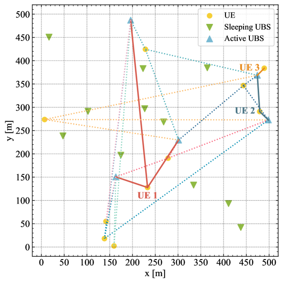
Figure 2: UBS sleeping and UE associations in FD-RAN ($M=16$, $K=10$).

We present a visual representation of UE association and UBS sleeping in Fig. 2. Facilitated by the proposed TriMSM algorithm, a cluster of UBSs is assigned to serve each UE, strategically placing underutilized UBSs into sleep mode to conserve energy. Notably, cluster size varies and is capped at $L$, aiming at maximizing energy efficiency.

VIII-C Energy Efficiency versus Different Architectures

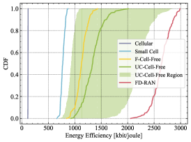
(a) CDF curves of energy efficiency ($M=16$, $K=5$).

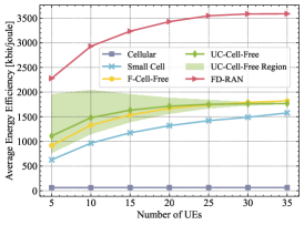
(b) Average energy efficiency versus different number of UEs ($M=16$).

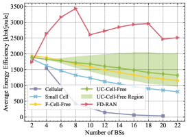
(c) Average energy efficiency versus different number of UBSs ($K=10$).

Figure 3: Energy efficiency versus different architectures.

Fig. 3 illustrates the energy efficiency versus different architectures. The cumulative distribution function (CDF) curves for energy efficiency are displayed in Fig. 3a. FD-RAN consistently outperforms all other existing architectures, exhibiting energy efficiency values 22.7, 3.40, 2.34, and 1.97 times higher than those of cellular, small cell, F-Cell-Free, and UC-Cell-Free, respectively. Notably, even in the best-case of UC-Cell-Free, the FD-RAN architecture maintains a significant 18.9% advantage in energy efficiency. Fig. 3b presents the average energy efficiency with varying numbers of UEs. As the number of UEs increases, the energy efficiency initially rises but gradually reaches a saturation point in most cases. This is primarily due to the almost full utilization of UBSs and the saturation of UE rate caused by limited network capacity. Notably, FD-RAN consistently outperforms the other architectures, with its superiority becoming even more pronounced as the number of UEs increases. This advantage stems from its centralized gains of BBUs. Fig. 3c illustrates the average energy efficiency versus the number of UBSs. Generally, as the number of BSs increases, the energy efficiency of most architectures decreases. However, in UC-Cell-Free and FD-RAN, the introduction of BS sleeping helps effectively manage the rising energy consumption of additional BSs, resulting in higher energy efficiency. This effect of BS sleeping is evident as shown in the UC-Cell-Free Region. The sharp drop of energy efficiency in FD-RAN will be explained in Section VIII-E. Furthermore, FD-RAN consistently outperforms other architectures except in cases with 2 UBSs ($M=2$). This deviation can be attributed to the additional cooling energy required in centralized BBU but the diminished centralized gain, only when $M$ is quite small. Based on the findings, FD-RAN’s remarkable energy efficiency stems from a flexible BS sleeping mechanism, enabled by its fully decoupled architecture, personalized service adaptability, and centralized gain.

Fig. 6 illustrates the QoS violations across different architectures. While F-Cell-Free delivers a commendable performance, it neglects to address the constraints (31e) and (31d), rendering it impractical. FD-RAN consistently provides superior QoS guarantees in most cases, while UC-Cell-Free benefits from mirrored UE association. However, in resource-constrained settings (e.g., $K=30$ and $35$ for $M=16$, and $M=4$ for $K=10$), cellular networks perform better. This is because, compared to single-connectivity in cellular, multi-connectivity in such scenario yields less gain and can result in uneven resource distribution when maximizing energy efficiency.

VIII-D Effectiveness of Proposed Algorithms

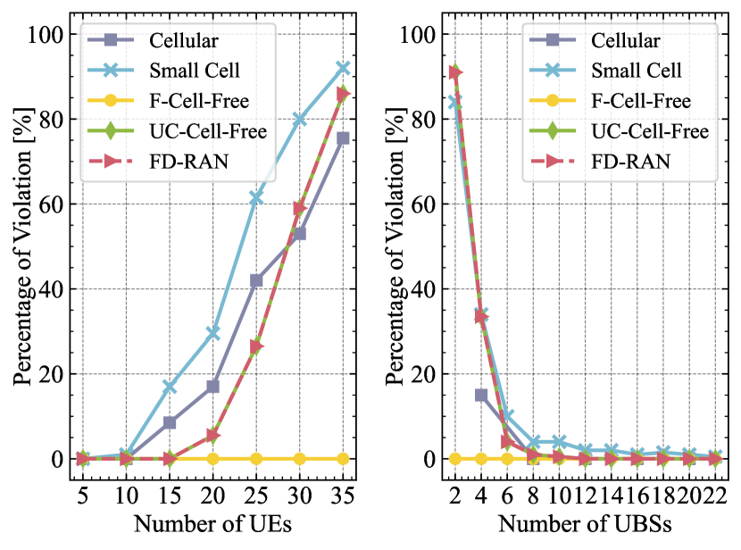
Figure 4: QoS violation percentage versus different architectures (with different number of UEs ($M=16$) and UBSs ($K=10$)).

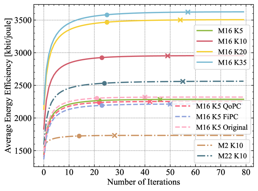
Figure 5: Convergence of SLMDB algorithm versus different algorithms, number of UEs and UBSs.

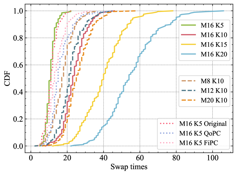
Figure 6: Swap times of TriMSM algorithm versus different algorithms, number of UEs and UBSs.

Fig. 6 illustrates the convergence curves of the SLMDB algorithm across different power control algorithms, numbers of UEs and UBSs. Solid and cross markers denote energy efficiency variation points of 1e-3 and 1e-4, respectively. The lines depict convergence behavior in TriMSM with EIPC unless stated otherwise. Various power control algorithms in TriMSM show similar convergence patterns, with original TriMSM having the best and FiPC the slowest convergence. Although SLMDB’s convergence slows with more UEs or UBSs, the impact remains relatively minor. Typically, about 20 steps suffice to reach the 1e-3 point. Thus, the SLMDB algorithm demonstrates robust convergence across diverse scenarios while maintaining good speed.

Fig. 6 shows the CDF of swap times for the TriMSM algorithm across various power control algorithms, numbers of UEs, and UBSs. The lines depict convergence behavior in TriMSM with EIPC unless stated otherwise. Notably, TriMSM with EIPC and original TriMSM exhibit similar swap times, generally with the fewest swaps, while FiPC has more swaps, and QoPC has the most. Despite the increasing UEs or UBSs, swap times in all cases stay within acceptable limits, averaging at most 55 swaps. Thus, Fig. 6 highlights manageable swap times for the TriMSM algorithm, even in large-scale network environments.

To evaluate computational time, we compare the original TriMSM algorithm with three low-complexity alternatives, employing only a single processing core. As depicted in Fig. 9, the results reveal that the original TriMSM algorithm suffers from notably high elapsed times, rendering it unsuitable for large-scale network applications, even when considering parallelization capabilities. In contrast, the three low-complexity alternatives demonstrate significantly reduced running times with nearly comparable performance. Among them, EIPC emerges as the top performer, achieving a 47.5-fold reduction in running time with just a 1.61% loss in performance. The other two alternatives also show lower but notably good performance.

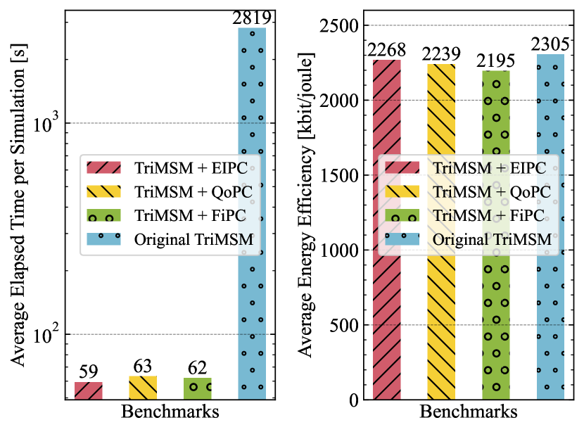
Figure 7: Average elapsed time (left) and average energy efficiency (right) comparison of TriMSM algorithms ($M=16$, $K=5$).

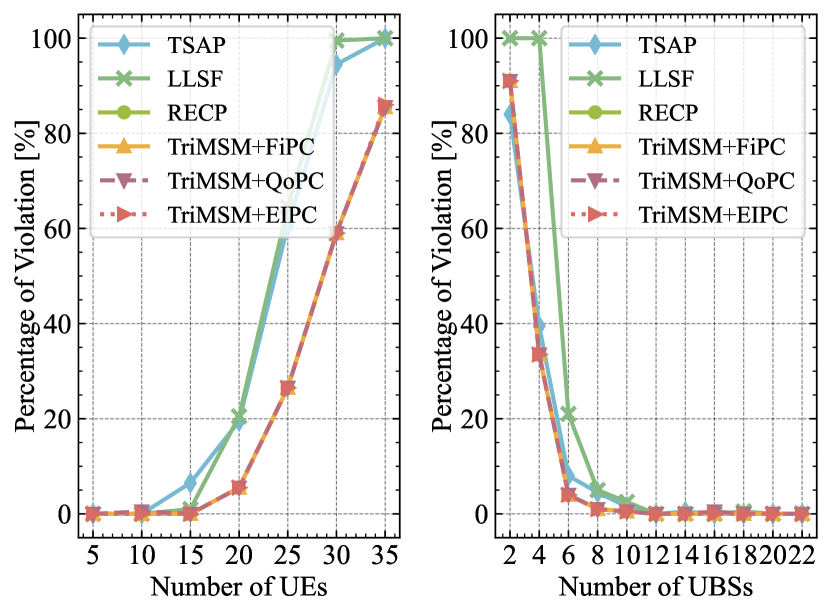
Figure 8: QoS violation percentage versus different algorithms (with different number of UEs ($M=16$) and UBSs ($K=10$)).

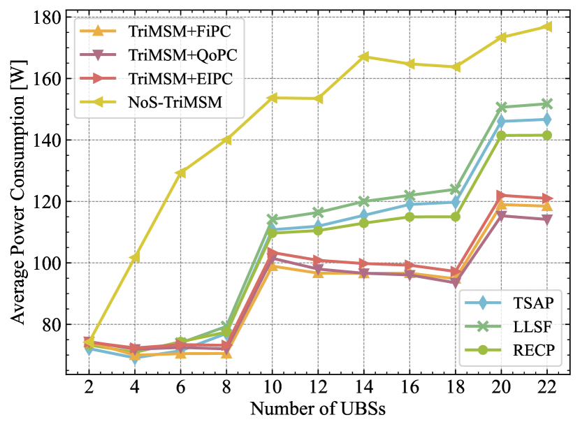
Figure 9: Average power consumption of algorithms versus different number of UBSs ($K=10$).

VIII-E Energy Efficiency versus Different Algorithms

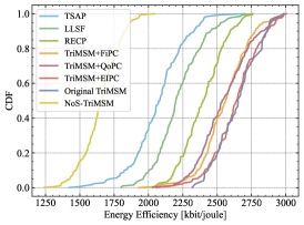
(a) CDF curves of energy efficiency ($M=16$, $K=5$).

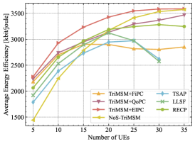
(b) Average energy efficiency versus different number of UEs ($M=16$).

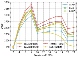
(c) Average energy efficiency versus different number of UBSs ($K=10$).

Figure 10: Energy efficiency versus different algorithms.

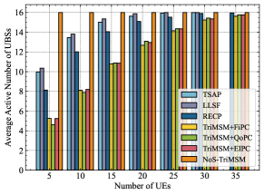
(a) Different number of UEs ($M=16$).

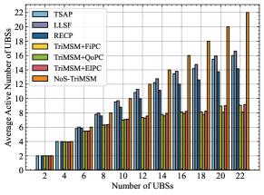
(b) Different number of UBSs ($K=10$).

Figure 11: Average active number of UBSs versus different algorithms.

Fig. 10 illustrates the energy efficiency versus different algorithms. Fig. 10a displays the CDF curves of energy efficiency, revealing that TriMSM algorithms exhibit the best performance, followed by peer algorithms, with the no-sleep algorithm performing the worst. The worst performing proposed algorithm achieves energy efficiency 6.60% and 23.4% higher than the best and worst peer algorithms, respectively. Notably, NoS-TriMSM exhibits the lowest efficiency, showing a 1.59-fold decrease in energy efficiency compared to TriMSM with sleeping, emphasizing the benefits of BS sleeping. Within the TriMSM algorithms, the original TriMSM demonstrates the best performance, while EIPC shows almost identical performance. FiPC and QoPC exhibit a minor performance gap. The average energy efficiency concerning the number of UEs is illustrated in Fig. 10b. The energy efficiency of algorithms initially rises and then declines with an increasing number of UEs, except for the TriMSM algorithms. This trend is attributed to excessive and redundant UBS utilization in peer algorithms, evident in Fig. 11a. TriMSM with EIPC consistently demonstrates the highest energy efficiency, with NoS-TriMSM gradually approaching it as the number of UEs increases due to nearly all UBS utilization. However, TriMSM with FiPC and QoPC exhibits less satisfactory energy efficiency. As depicted in Fig. 11b, the UBS utilization among TriMSM algorithms is similar, suggesting that the decline in performance stems from their suboptimal power control strategies. In Fig. 10c, the average energy efficiency concerning the number of UBSs is depicted. There is a significant decline in energy efficiency when the number of UBSs increases tenfold, linked to FD-RAN’s power consumption, as evident in Fig. 9. This phenomenon can be explained by (21), where every $\lambda\zeta=10$ points experience a notable surge in power consumption. The TriMSM serial algorithms exhibit the highest growth rates of energy efficiency within the small intervals, with EIPC consistently being the most efficient choice. This superiority stems from effective BS sleeping and centralized gain, leading to reduced power consumption, as evidenced in Fig. 9. Notably, TriMSM with FiPC exhibits subpar energy efficiency in heavy-load scenarios ($M<14$), whereas NoS-TriMSM performs well under heavy loads ($M<6$) but experiences declining performance as the load decreases.

Fig. 11 presents the average active number of UBSs across different algorithms. NoS-TriMSM engages all available UBSs, while TSAP, LLSF, and RECP successively utilize fewer UBSs. Conversely, our proposed TriMSM algorithms prioritize the sleeping of most UBSs. Notably, the most efficient TriMSM variant, EIPC, doesn’t feature the fewest active UBSs. Therefore, optimizing energy efficiency should consider a balance between energy consumption and achievable UE rates, rather than merely minimizing the number of active UBSs. As depicted in Fig. 11a, as the number of UEs increases, more UBSs are utilized. Different from peer algorithms needing many UBSs all the time, TriMSM algorithms can efficiently put more UBSs to sleep, dynamically adapting to the number of UEs. In Fig. 11a, as the number of UEs increases, more UBSs are utilized. Unlike peer algorithms constantly requiring numerous active UBSs, TriMSM algorithms can efficiently put more UBSs to sleep, dynamically adapting to the number of UEs. Meanwhile, Fig. 11b illustrates a rise in active UBSs concerning UBS number. Notably, the growth rate of TriMSM algorithms is notably restrained compared to the near-linear increments seen in peer algorithms. This observation sheds light on their superior energy efficiency, as demonstrated in Fig. 10.

Fig. 9 depicts QoS violations across various algorithms. LLSF registers the highest QoS violation rate, while TSAP shows fewer violations. Notably, both RECP and TriMSM algorithms share the same lowest percentage of QoS violations, since RECP serves as the foundational algorithm for TriMSM algorithms. This emphasizes the effectiveness of TriMSM in maintaining QoS.

VIII-F Energy Efficiency versus Real Traffic

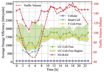
(a) Comparison of different architectures.

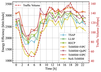
(b) Comparison of different algorithms.

Figure 12: Energy efficiency versus real traffic.

We use the dataset from [38], comprising real-world spatiotemporal traffic data. The dataset consists of 100$\times$100 cells over 62 days, recorded at hourly intervals. To assess FD-RAN and our proposed algorithms’ real-world performance while maintaining generality, we aggregate the traffic from these cells into 5$\times$5 regions, partitioning the simulation area accordingly. If a region’s traffic constitutes less than 20% of the total, its traffic is set to 0. Each region is represented by a single UE placed at its center. Moreover, the total traffic across regions fluctuates over time, shown by the dotted line in Fig. 12, with maximum traffic scaled to 160 Mbps.

We evaluate the energy efficiency of architectures and algorithms using real-world traffic data in Fig. 12a and Fig. 12b, respectively. Generally, the energy efficiency of these architectures and algorithms exhibits fluctuations corresponding to variations in real traffic, indicating their adaptability across diverse scenarios. The performance ranking depicted in Fig. 12 aligns with the aforementioned observations. However, FD-RAN and TriMSM with EIPC do not consistently exhibit the highest performance due to the unique characteristics of the real traffic scenario, which might not fully represent their overall capabilities. Nonetheless, FD-RAN and TriMSM with EIPC remain preferable choices from a broader perspective.

IX Conclusion

In this paper, we have investigated energy-efficient uplink FD-RAN by flexible BS sleeping and resource cooperation. We have developed a holistic energy consumption model for FD-RAN and defined a bi-level problem of maximizing energy efficiency. Subsequently, we have decomposed this bi-level problem into a lower-level power control problem and an upper-level joint UE association and BS sleeping problem, which have been tackled by the successive lower-bound maximization-based Dinkelbach’s algorithm and the modified many-to-many matching algorithm, along with low-complexity realizations, respectively. The extensive simulation results have showcased the heightened energy efficiency of FD-RAN and the effectiveness of the proposed algorithms. These outcomes reveal that the predominant sources of energy efficiency gains in FD-RAN stem from a flexible BS sleeping mechanism enabled by the fully decoupled architecture, the flexibility of personalized services, and centralized gains. For the future work, we will investigate the downlink scenario in FD-RAN to further explore the green potential of this architecture.

Appendix A Proof of Lemma 1

Proof:

Considering that the number of antennas, bandwidth, quantization, spectral efficiency, and streams are typically fixed in the real world, we can express the power consumption of UBSs as a combination of fixed and varying parts, as follows:

$$\sum_{m\in\mathcal{M_{A}}}P_{m}^{\mathrm{BS}} =\sum_{m\in\mathcal{M_{A}}}P_{m}^{\mathrm{BS_{fix}}}+\sum_{m\in\mathcal{M_{A}}}\sum_{j\in\mathcal{J}_{\mathrm{BBU}}}P_{m}^{\mathrm{BBU}_{j,\mathrm{fix}}}$$

$$+\sum_{m\in\mathcal{M_{A}}}\sum_{j\in\mathcal{J}_{\mathrm{BBU}}}P_{m}^{\mathrm{BBU}_{j,\mathrm{ref}}}\left(\frac{Ld_{m}}{Ld_{m}^{\mathrm{ref}}}\right)^{s_{m}^{j,Ld}},$$ (50)

where the first two terms represent the fixed energy of the BSs (excluding BBUs) and BBUs, respectively. The last term corresponds to the varying energy of BBUs, which depends on the load and can be further expanded as:

$$\sum_{m\in\mathcal{M_{A}}}\left(\sum_{j\in\mathcal{J^{\prime}}_{\mathrm{BBU}}}P_{m}^{\mathrm{BBU}_{j,\mathrm{ref}}}+\sum_{j\in\mathcal{J^{\prime\prime}}_{\mathrm{BBU}}}P_{m}^{\mathrm{BBU}_{j,\mathrm{ref}}}\frac{Ld_{m}^{s_{m}^{j,Ld}}}{{Ld_{m}^{\mathrm{ref}}}^{s_{m}^{j,Ld}}}\right),$$ (51)

where $s_{m}^{j,Ld}=0$ for $j\in\mathcal{J}_{\mathrm{BBU}}^{\prime}$, and $s_{m}^{j,Ld}=1$ or $0.5$ for $j\in\mathcal{J}_{\mathrm{BBU}}^{\prime\prime}$. To simplify the expression, we set $s_{m}^{j,Ld}=1$ for $j\in\mathcal{J}_{\mathrm{BBU}}^{\prime\prime}$, and the varying part of (51) can be calculated as:

$$\sum_{m\in\mathcal{M_{A}}}\sum_{j\in\mathcal{J}^{\prime\prime}_{\mathrm{BBU}}}P_{m}^{\mathrm{BBU}_{j,\mathrm{ref}}}\frac{Ld_{m}}{{Ld_{m}^{\mathrm{ref}}}}$$

$$\overset{(a)}{=} \sum_{j\in\mathcal{J}^{\prime\prime}_{\mathrm{BBU}}}P_{m}^{\mathrm{BBU}_{j,\mathrm{ref}}}\sum_{m\in\mathcal{M_{A}}}\frac{R^{\prime}_{m}}{{R^{\prime}_{m,\mathrm{ref}}}}$$

$$\overset{(b)}{=} \sum_{k\in\mathcal{K}}\frac{R_{k}}{{R_{k,\mathrm{ref}}}}\sum_{j\in\mathcal{J}^{\prime\prime}_{\mathrm{BBU}}}P_{m}^{\mathrm{BBU}_{j,\mathrm{ref}}},$$ (52)

where step $(a)$ swaps the order of summation and substitutes (27), while step $(b)$ is obtained by utilizing (28) and swapping the order of summation. By combining equations (50)-(52), and denoting the summation of all fixed energy as $\sum_{m\in\mathcal{M_{A}}}P_{m}^{\mathrm{BS}_{\mathrm{fix}}}$ and $\sum_{j\in\mathcal{J}^{\prime\prime}_{\mathrm{BBU}}}P_{m}^{\mathrm{BBU}_{j,\mathrm{ref}}}$ as $P_{\mathrm{trf}}$, we complete the proof. $\blacksquare$

Appendix B Proof of Lemma 3

Proof:

Let $\boldsymbol{\rho}\in\mathbf{P}$ denote the domain formed by constraints (31c) and (34). By introducing the auxiliary variable $\pi$, the problem $\mathcal{P}_{l}$ can be equivalently expressed as:

$$\max_{\boldsymbol{\rho}\in\mathbf{P}}~{}\pi\quad\text{s.t.}~{}\pi-\frac{\sum_{k\in\mathcal{K}}R_{k}\left(\boldsymbol{\rho}\right)}{P_{\mathrm{N}}\left(\boldsymbol{\rho},\left\{R_{k}\left(\boldsymbol{\rho}\right)\right\}\right)}\leq 0.$$ (53)

It is worth noting that $P_{\mathrm{N}}\left(\boldsymbol{\rho},\left\{R_{k}\left(\boldsymbol{\rho}\right)\right\}\right)>0$, allowing us to rewrite the problem as:

$$\max_{\boldsymbol{\rho}\in\mathbf{P}}~{}\pi$$ (54a)

$$\text{s.t.}~{}\pi P_{\mathrm{N}}\left(\boldsymbol{\rho},\left\{R_{k}\left(\boldsymbol{\rho}\right)\right\}\right)-\sum_{k\in\mathcal{K}}R_{k}\left(\boldsymbol{\rho}\right)\leq 0.$$ (54b)

As demonstrated in [39], the above problem is equivalent to finding the root of the following nonlinear function:

$$F\left(\pi\right)=\max_{\boldsymbol{\rho}\in\mathbf{P}}~{}\sum_{k\in\mathcal{K}}R_{k}\left(\boldsymbol{\rho}\right)-\pi P_{\mathrm{N}}\left(\boldsymbol{\rho},\left\{R_{k}\left(\boldsymbol{\rho}\right)\right\}\right),$$ (55)

, thus, the condition for global optimality is given by:

$$F\left(\pi^{\ast}\right)=0.$$ (56)

This completes the proof. $\blacksquare$

Appendix C Proof of Lemma 4

Proof:

The functions $\hat{f}_{k}\left(\boldsymbol{\rho},\boldsymbol{\rho}_{0}\right)$ and $\hat{g}_{k}\left(\boldsymbol{\rho},\boldsymbol{\rho}_{0}\right)$ represent the first-order Taylor approximations of $f_{k}\left(\boldsymbol{\rho}\right)$ and $g_{k}\left(\boldsymbol{\rho}\right)$ at the point $\boldsymbol{\rho}_{0}$, respectively. According to the properties of concave functions, we have $\hat{f}_{k}\left(\boldsymbol{\rho},\boldsymbol{\rho}_{0}\right)\geq f_{k}\left(\boldsymbol{\rho}\right)$ and $\hat{g}_{k}\left(\boldsymbol{\rho},\boldsymbol{\rho}_{0}\right)\geq g_{k}\left(\boldsymbol{\rho}\right)$. Combining equations (37a), (40), and (41), we obtain $\hat{R}\left(\boldsymbol{\rho},\boldsymbol{\rho}_{0}\right)\geq R_{k}\left(\boldsymbol{\rho}\right)$ and $\overline{R}\left(\boldsymbol{\rho},\boldsymbol{\rho}_{0}\right)\leq R_{k}\left(\boldsymbol{\rho}\right)$. Since $R_{k}\left(\boldsymbol{\rho}\right)\geq 0$ and $P_{N}\left(\boldsymbol{\rho}\right)\geq 0$, where $P_{N}\left(\boldsymbol{\rho}\right)$ is an affine function of $R_{k}\left(\boldsymbol{\rho}\right)$, we can easily deduce that $\overline{\mathrm{EE}}\left(\boldsymbol{\rho},\boldsymbol{\rho}_{0}\right)\leq\mathrm{EE}\left(\boldsymbol{\rho}\right)$. Furthermore, the equality of $\hat{f}_{k}\left(\boldsymbol{\rho},\boldsymbol{\rho}_{0}\right)\geq f_{k}\left(\boldsymbol{\rho}\right)$ and $\hat{g}_{k}\left(\boldsymbol{\rho},\boldsymbol{\rho}_{0}\right)\geq g_{k}\left(\boldsymbol{\rho}\right)$ holds if and only if $\boldsymbol{\rho}=\boldsymbol{\rho}_{0}$. Therefore, under the same condition, the equality $\overline{\mathrm{EE}}\left(\boldsymbol{\rho},\boldsymbol{\rho}_{0}\right)=\mathrm{EE}\left(\boldsymbol{\rho}\right)$ also holds. $\blacksquare$

Appendix D Proof of Theorem 1

Proof:

According to [40, Theorem 1] and [40, Corollary 1], when [40, Assumption 1] holds and the level set of $\mathrm{EE}\left(\boldsymbol{\rho}\right)$ is compact, Theorem 1 holds. The fulfillment of these assumptions is proven as follows:

By defining the domain $\boldsymbol{\rho}\in\mathbf{P}$ as the set of constraints (31c) and (34), the following result can be readily derived based on Lemma 4:

$$\overline{\mathrm{EE}}\left(\boldsymbol{\rho},\boldsymbol{\rho}\right)=\mathrm{EE}\left(\boldsymbol{\rho}\right),~{}\forall\boldsymbol{\rho}\in\mathbf{P},$$ (57a)

$$\overline{\mathrm{EE}}\left(\boldsymbol{\rho},\boldsymbol{\rho}^{\prime}\right)\leq\mathrm{EE}\left(\boldsymbol{\rho}\right),~{}\forall\boldsymbol{\rho},\boldsymbol{\rho}^{\prime}\in\mathbf{P}.$$ (57b)

Furthermore, the following properties can be easily verified based on the characteristics of $\mathrm{EE}\left(\boldsymbol{\rho}\right)$:

$$\frac{\partial\overline{\mathrm{EE}}\left(\boldsymbol{\rho},\boldsymbol{\rho}^{\prime}\right)}{\partial\boldsymbol{\rho}}\bigg{|}_{\boldsymbol{\rho}\to\boldsymbol{\rho}^{\prime}}=\frac{\partial\mathrm{EE}\left(\boldsymbol{\rho}\right)}{\partial\boldsymbol{\rho}}\bigg{|}_{\boldsymbol{\rho}\to\boldsymbol{\rho}^{\prime}},~{}\forall\boldsymbol{\rho}\in\mathbf{P},$$ (57c)

$$\overline{\mathrm{EE}}\left(\boldsymbol{\rho},\boldsymbol{\rho}^{\prime}\right)\text{ is continuous in }\left(\boldsymbol{\rho},\boldsymbol{\rho}^{\prime}\right),$$ (57d)

$$\text{Level set of }\mathrm{EE}\left(\boldsymbol{\rho}\right)\text{ is compact}.$$ (57e)

$\blacksquare$

References

- [1] B. Mao, F. Tang, Y. Kawamoto, and N. Kato, “AI Models for Green Communications Towards 6G,” IEEE Commun. Surv. Tutor., vol. 24, no. 1, pp. 210–247, 2022.
- [2] “2022 ESG addendum,” Vodafone, Tech. Rep., May 2022.
- [3] IIMT. Union, “IMT traffic estimates for the years 2020 to 2030,” Rep. ITU, vol. 2370, 2015.
- [4] Q. Yu, H. Zhou, J. Chen, Y. Li, J. Jing, J. J. Zhao, B. Qian, and J. Wang, “A Fully-Decoupled RAN Architecture for 6G Inspired by Neurotransmission,” J. Commun. Inf. Netw., vol. 4, no. 4, pp. 15–23, Dec. 2019.
- [5] J. Zhao, Q. Yu, B. Qian, K. Yu, Y. Xu, H. Zhou, and X. Shen, “Fully-Decoupled Radio Access Networks: A Resilient Uplink Base Stations Cooperative Reception Framework,” IEEE Trans. Wirel. Commun., pp. 1–1, 2023.
- [6] W. Dinkelbach, “On Nonlinear Fractional Programming,” Manag. Sci., vol. 13, no. 7, pp. 492–498, Mar. 1967.
- [7] B. Debaillie, C. Desset, and F. Louagie, “A Flexible and Future-Proof Power Model for Cellular Base Stations,” in IEEE Veh Technol Conf, May 2015, pp. 1–7.
- [8] G. Auer, V. Giannini, C. Desset, I. Godor, P. Skillermark, M. Olsson, M. A. Imran, D. Sabella, M. J. Gonzalez, O. Blume, and A. Fehske, “How much energy is needed to run a wireless network?” IEEE Wirel. Commun., vol. 18, no. 5, pp. 40–49, Oct. 2011.
- [9] C. Desset, B. Debaillie, V. Giannini, A. Fehske, G. Auer, H. Holtkamp, W. Wajda, D. Sabella, F. Richter, M. J. Gonzalez, H. Klessig, I. Gódor, M. Olsson, M. A. Imran, A. Ambrosy, and O. Blume, “Flexible power modeling of LTE base stations,” in IEEE Wireless Commun. Networking Conf. WCNC, Apr. 2012, pp. 2858–2862.
- [10] Y. Xu, H. Xie, Q. Wu, C. Huang, and C. Yuen, “Robust Max-Min Energy Efficiency for RIS-Aided HetNets With Distortion Noises,” IEEE Trans. Commun., vol. 70, no. 2, pp. 1457–1471, Feb. 2022.
- [11] M. Fiorani, S. Tombaz, J. Martensson, B. Skubic, L. Wosinska, and P. Monti, “Modeling energy performance of C-RAN with optical transport in 5G network scenarios,” J. Opt. Commun. Netw., vol. 8, no. 11, pp. B21–B34, Nov. 2016.
- [12] M. Bashar, K. Cumanan, A. G. Burr, H. Q. Ngo, E. G. Larsson, and P. Xiao, “Energy Efficiency of the Cell-Free Massive MIMO Uplink With Optimal Uniform Quantization,” IEEE Trans. Green Commun. Netw., vol. 3, no. 4, pp. 971–987, Dec. 2019.
- [13] T. Van Chien, E. Bjornson, and E. G. Larsson, “Joint Power Allocation and Load Balancing Optimization for Energy-Efficient Cell-Free Massive MIMO Networks,” IEEE Trans. Wirel. Commun., vol. 19, no. 10, pp. 6798–6812, Oct. 2020.
- [14] J. Wu, Y. Zhang, M. Zukerman, and E. K.-N. Yung, “Energy-Efficient Base-Stations Sleep-Mode Techniques in Green Cellular Networks: A Survey,” IEEE Commun. Surv. Tutor., vol. 17, no. 2, pp. 803–826, 2015.
- [15] J. Lin, Y. Chen, H. Zheng, M. Ding, P. Cheng, and L. Hanzo, “A Data-driven Base Station Sleeping Strategy Based on Traffic Prediction,” IEEE Trans. Netw. Sci. Eng., pp. 1–1, 2021.
- [16] M. Masoudi, E. Soroush, J. Zander, and C. Cavdar, “Digital Twin Assisted Risk-Aware Sleep Mode Management Using Deep Q-Networks,” IEEE Trans. Veh. Technol., vol. 72, no. 1, pp. 1224–1239, Jan. 2023.
- [17] T. Zhou, Y. Fu, D. Qin, X. Li, and C. Li, “Joint User Association and BS Operation for Green Communications in Ultra-Dense Heterogeneous Networks,” IEEE Trans. Veh. Technol., pp. 1–14, 2023.
- [18] F. Salahdine, J. Opadere, Q. Liu, T. Han, N. Zhang, and S. Wu, “A survey on sleep mode techniques for ultra-dense networks in 5G and beyond,” Comput. Netw., vol. 201, p. 108567, Dec. 2021.
- [19] T. Ma, H. Zhou, B. Qian, N. Cheng, X. Shen, X. Chen, and B. Bai, “UAV-LEO Integrated Backbone: A Ubiquitous Data Collection Approach for B5G Internet of Remote Things Networks,” IEEE J. Sel. Areas Commun., vol. 39, no. 11, pp. 3491–3505, Nov. 2021.
- [20] K. Shen and W. Yu, “Fractional Programming for Communication Systems—Part I: Power Control and Beamforming,” IEEE Trans. Signal Process., vol. 66, no. 10, pp. 2616–2630, May 2018.
- [21] N. Huang, C. Dou, Y. Wu, L. Qian, and R. Lu, “Energy-Efficient Integrated Sensing and Communication: A Multi-Access Edge Computing Design,” IEEE Wirel. Commun. Lett., pp. 1–1, 2023.
- [22] F. Guo, H. Lu, and Z. Gu, “Joint Power and User Grouping Optimization in Cell-Free Massive MIMO Systems,” IEEE Trans. Wirel. Commun., vol. 21, no. 2, pp. 991–1006, Feb. 2022.
- [23] B. Qian, T. Ma, Y. Xu, J. Zhao, K. Yu, Y. Wu, and H. Zhou, “Enabling Fully-Decoupled Radio Access with Elastic Resource Allocation,” IEEE Trans. Cogn. Commun. Netw., pp. 1–1, 2023.
- [24] B. Di, L. Song, and Y. Li, “Sub-Channel Assignment, Power Allocation, and User Scheduling for Non-Orthogonal Multiple Access Networks,” IEEE Trans. Wirel. Commun., vol. 15, no. 11, pp. 7686–7698, Nov. 2016.
- [25] E. Björnson, J. Hoydis, and L. Sanguinetti, “Massive MIMO Networks: Spectral, Energy, and Hardware Efficiency,” Found. Trends® Signal Process., vol. 11, no. 3-4, pp. 154–655, 2017.
- [26] X. Ge, J. Yang, H. Gharavi, and Y. Sun, “Energy Efficiency Challenges of 5G Small Cell Networks,” IEEE Commun. Mag., vol. 55, no. 5, pp. 184–191, May 2017.
- [27] G. Lim and L. J. Cimini, “Energy-efficient best-select relaying in wireless cooperative networks,” in Annu. Conf. Inf. Sci. Syst., CISS, Mar. 2012, pp. 1–6.
- [28] P. Hũu, M. A. Arfaoui, S. Sharafeddine, C. M. Assi, and A. Ghrayeb, “A Low-Complexity Framework for Joint User Pairing and Power Control for Cooperative NOMA in 5G and Beyond Cellular Networks,” IEEE Trans. Commun., vol. 68, no. 11, pp. 6737–6749, Nov. 2020.
- [29] A. Sinha, P. Malo, and K. Deb, “A Review on Bilevel Optimization: From Classical to Evolutionary Approaches and Applications,” IEEE Trans. Evol. Comput., vol. 22, no. 2, pp. 276–295, Apr. 2018.
- [30] K. TAMMER, “The application of parametric optimization and imbedding to the foundation and realization of a generalized primal decomposition approach,” appl. parametr. optim. imbedding found. realiz. gen. primal decompos. approach, vol. 35, pp. 376–386, 1987.
- [31] C. Isheden, Z. Chong, E. Jorswieck, and G. Fettweis, “Framework for Link-Level Energy Efficiency Optimization with Informed Transmitter,” IEEE Trans. Wirel. Commun., vol. 11, no. 8, pp. 2946–2957, Aug. 2012.
- [32] E. Bodine-Baron, C. Lee, A. Chong, B. Hassibi, and A. Wierman, “Peer Effects and Stability in Matching Markets,” in Algorithmic Game Theory, ser. Lecture Notes in Computer Science, G. Persiano, Ed. Berlin, Heidelberg: Springer, 2011, pp. 117–129.
- [33] K. Yu, Q. Yu, Z. Tang, J. Zhao, B. Qian, Y. Xu, H. Zhou, and X. Shen, “Fully-Decoupled Radio Access Networks: A Flexible Downlink Multi-connectivity and Dynamic Resource Cooperation Framework,” IEEE Trans. Wirel. Commun., pp. 1–1, 2022.
- [34] H. Q. Ngo, L.-N. Tran, T. Q. Duong, M. Matthaiou, and E. G. Larsson, “On the Total Energy Efficiency of Cell-Free Massive MIMO,” IEEE Trans. Green Commun. Netw., vol. 2, no. 1, pp. 25–39, Mar. 2018.
- [35] E. Björnson and L. Sanguinetti, “Scalable Cell-Free Massive MIMO Systems,” IEEE Trans. Commun., vol. 68, no. 7, pp. 4247–4261, Jul. 2020.
- [36] R. P. Antonioli, I. M. Braga, G. Fodor, Y. C. B. Silva, A. L. F. De Almeida, and W. C. Freitas, “On the Energy Efficiency of Cell-Free Systems with Limited Fronthauls: Is Coherent Transmission Always the Best Alternative?” IEEE Trans. Wirel. Commun., pp. 1–1, 2022.
- [37] D. López-Pérez, A. De Domenico, N. Piovesan, G. Xinli, H. Bao, S. Qitao, and M. Debbah, “A Survey on 5G Radio Access Network Energy Efficiency: Massive MIMO, Lean Carrier Design, Sleep Modes, and Machine Learning,” IEEE Commun. Surv. Tutor., vol. 24, no. 1, pp. 653–697, 2022.
- [38] C. Zhang, H. Zhang, J. Qiao, D. Yuan, and M. Zhang, “Deep Transfer Learning for Intelligent Cellular Traffic Prediction Based on Cross-Domain Big Data,” IEEE J. Sel. Areas Commun., vol. 37, no. 6, pp. 1389–1401, Jun. 2019.
- [39] S. Schaible and T. Ibaraki, “Fractional programming,” Eur. J. Oper. Res., vol. 12, no. 4, pp. 325–338, Apr. 1983.
- [40] M. Razaviyayn, M. Hong, and Z. Q. Luo, “A unified convergence analysis of block successive minimization methods for nonsmooth optimization,” SIAM J. Optim., vol. 23, no. 2, pp. 1126–1153, 2013.