Error analysis of BDF 1–6 time-stepping methods for the transient Stokes problem:
Velocity and pressure estimates

Abstract

We present a new stability and error analysis of fully discrete approximation schemes for the transient Stokes equation. For the spatial discretization, we consider a wide class of Galerkin finite element methods which includes both inf-sup stable spaces and symmetric pressure stabilized formulations. We extend the results from Burman and Fernández [SIAM J. Numer. Anal., 47 (2009), pp. 409-439] and provide a unified theoretical analysis of backward difference formulae (BDF methods) of order 1 to 6. The main novelty of our approach lies in deriving optimal-order stability and error estimates for both the velocity and the pressure using Dahlquist’s $G$-stability concept together with the multiplier technique introduced by Nevanlinna and Odeh and recently by Akrivis et al. [SIAM J. Numer. Anal., 59 (2021), pp. 2449-2472]. When combined with a method dependent Ritz projection for the initial data, unconditional stability can be shown while for arbitrary interpolation, pressure stability is subordinate to the fulfilment of a mild inverse CFL-type condition between space and time discretizations.

65M12, 65M15, 65M60, 76M10

1 Introduction

Let $\Omega\subset\mathbb{R}^{d},\;d\in\{2,3\}$ be a Lipschitz domain with boundary $\partial\Omega$ and $J:=(0,T),\;T>0$ be a finite time interval. We consider the transient Stokes equation as a simplified prototype problem for the time-dependent flow of an incompressible fluid: find ${\boldsymbol{u}}\colon\Omega\times J\to\mathbb{R}^{d}$ and $p\colon\Omega\times J\to\mathbb{R}$ such that

(1) $$\left\{\begin{aligned} ~{}\partial_{t}{\boldsymbol{u}}-\nu\Delta{\boldsymbol{u}}+\nabla p=&\ {\boldsymbol{f}}&&\qquad\text{ in }\Omega\times J,\\ \nabla\cdot{\boldsymbol{u}}=&\ 0&&\qquad\text{ in }\Omega\times J,\\ {\boldsymbol{u}}=&\ 0&&\qquad\text{ on }\partial\Omega\times J,\\ {\boldsymbol{u}}(\cdot,0)=&\ {\boldsymbol{u}}_{0}&&\qquad\text{ in }\Omega,\end{aligned}\right.$$

where ${\boldsymbol{f}}\colon\Omega\times J\to\mathbb{R}$ is an external force field, ${\boldsymbol{u}}_{0}\colon\Omega\to\mathbb{R}^{d}$ is the given initial, divergence-free velocity field and $\nu>0$ denotes a constant kinematic viscosity.

1.1 State of the art

This paper is concerned with the stability and error analysis of fully discrete formulations of the transient Stokes equation (1). We analyze BDF methods of order $1$–$6$ in combination with a large class of Galerkin finite element methods which utilize so-called symmetric pressure stabilizations. For the classical analysis of inf-sup stable Galerkin finite elements paired with lower order time stepping schemes, we refer to [23, Part XIV] and [29, Chapter 3–7]. Due to the complexity of constructing mixed finite elements which provably satisfy a discrete uniform inf-sup condition, stabilized methods have been developed and analyzed which circumvent the inf-sup condition and allow for equal-order interpolation spaces. Here, a main challenge in the design and theoretical analysis of the fully discrete transient Stokes problem is the intricate interplay between the selected stabilized space discretization of the Stokes operator and the chosen time stepping scheme. For instance, the popular strongly consistent Pressure Stabilized Petrov–Galerkin (PSPG) method, proposed in [28], introduces a coupling between the time derivative of the velocity and the pressure gradient in the transient case. As a result, pressure instabilities can occur when an inverse parabolic Courant–Friedrichs–Lewy (CFL) condition between the time step $\tau$ and the mesh size $h$ in the form $\tau>Ch^{2}/\nu$ is not satisfied. Moreover, $H^{1}$-conform discrete velocity spaces are also subject to an inverse parabolic or hyperbolic CFL condition for BDF-1 or BDF-2 schemes, respectively, see [13]. These small time step instabilities can be avoided by a careful construction of the initial data [30].

As an alternative to residual-based stabilization approaches such as the PSPG method, a number of weakly consistent symmetric pressure stabilizations have been proposed. They have the favorable property that they typically commute with the discretization of both temporal operators and optimal control problems. Instances include the pressure gradient stabilization by Brezzi and Pitkäranta [10], Orthogonal Subscale Stabilizations (OSS) [17], methods based on certain pressure projections such as the Local Projection Stabilization (LPS) [8] or the method by Dohrmann and Bochev [20], and methods based on a Continuous Interior Penalty (CIP) for $H^{1}$-conform discrete pressure variable [14]. In [12], all the aforementioned symmetric pressure stabilized formulations were put into a general abstract framework to provide a unified analysis of fully discrete formulations employing either BDF-1, BDF-2 or Crank-Nicolson time stepping methods. Optimal convergence rates for the velocity and pressure are derived if a suitable Ritz projection is used for the initial data, otherwise a weak inverse CFL condition of the form $\tau>Ch^{2k}$ must be satisfied, where $k$ is the polynomial degree of the employed velocity approximation space. The analysis was later expanded to the full Navier–Stokes case in [24].

The majority of analyses of either inf-sup stable or stabilized formulations of the transient Stokes equation are restricted to at most second order in time schemes such as BDF-1, BDF-2 or Crank-Nicolson methods. Notable exceptions are discontinuous Galerkin time stepping methods, and we refer to [16] and [1] for the case of inf-sup stable and LPS stabilized spatial discretizations, respectively, and to [9] for an analysis which involves inf-sup stable spaces and only minimal regularity assumptions on the data. To the best of our knowledge, the only available analysis of higher order BDF methods for the transient Stokes problem is provided in [33], which considers BDF-$q$ schemes up to order 5 on both stationary and moving domains. The analysis is quite elaborate as it requires the solution of a nonlinear system of coefficients that are needed to guarantee that certain telescopic properties of the discrete time derivative and a positivity condition for the energy bilinear form are upheld when suitable discrete velocity test functions are inserted into the momentum equation. The coefficients do not come in close form and are computed numerically for $q=3,4,5$ while the case $q=6$ could not be treated. Most importantly, the described approach does not provide stability or error estimates for the pressure approximation. However, in recent years, Dahlquist’s $G$-stability theory [19] in connection with the multiplier technique devised by Nevanlinna and Odeh [37] has developed into a powerful technique to analyse higher order BDF time stepping methods for parabolic problems in an elegant and unified way. Originally developed for the stability analysis of linear multistep methods for contractive nonlinear ordinary differential equations, the use of these techniques for parabolic PDEs using BDF up to order 5 has been first presented in [34]. The extension to quasi-linear parabolic PDEs is due to [7]. These results have been successively extended to a larger class of problems (see [6, 5, 3]) and the original estimates by Nevanlinna ([35, 36]) were sharpened in [4]. The case of BDF-6 is treated in [2]. We refer to [25, 26] for the theory of BDF methods and $G$-stability. For PDEs, fully discrete error analysis of high-order BDF methods utilizing approaches similar to what is done in this text are considered in [34] with application to moving surfaces, while [31, 32] and [3] used the multiplier techniques but testing with the time derivatives. The multiplier technique is also used in the analysis of the so called Scalar Auxiliary Variable (SAV) method to prove convergence of higher order time stepping schemes, see for example [27].

1.2 New contributions and outline of the paper

To the best of our knowledge there is no fully discrete analysis of the transient Stokes problem for BDF-q from 1 to 6 providing stability and optimal error estimates for both velocity and pressure. The goal of our paper is therefore to close this gap, and at the same time, we wish to exemplify how the concept of $G$-stability and multiplier techniques can be used to analyze time-dependent saddle point problems by mimicking arguments from the stability analysis of the continuous problems. We start therefore by reviewing the weak formulation of the transient Stokes problem in Section 2, with a particular emphasis on how bounds for the velocity and its time-derivate in the respectively $L^{2}$–$H^{1}$ and $L^{2}$–$L^{2}$ norms lead to a pressure estimate in the $L^{2}$–$L^{2}$ norm via the inf-sup condition. Section 3 then provides details on the fully discrete formulation of the transient Stokes problem and collects the relevant theoretical results for its analysis. We recall the spatial discretization framework from [12] which includes a large family of Galerkin finite element methods including symmetric pressure stabilized and inf-sup stable formulations. Each spatial discretization yields a method-dependent Ritz projection that will play an important role later in the analysis. For the discretization in time, we use BDF-$q$ methods of order $q=1,\dotsc,6$, and we recall the main results from Dahlquist’s theory of $G$-stability [19] and multiplier techniques by Nevanlinna–Odeh [37] and Akrivis et al. [2] that will be crucial for the subsequent stability analysis.

In Section 4, we start the development of the new stability analysis of the fully discrete transient Stokes problem. As a first step, $L^{\infty}$ in time bounds for the velocity and pressure with respect to $H^{1}$-norm for the velocity and the stabilization induced semi-norm for the pressure are established by combining $G$-stability with the Nevanlinna–Odeh multiplier technique, similar to analysis in [34, 7]. But in contrast to the parabolic case, we also exploit the stabilized discrete formulation of the incompressibility constraint to recast certain pressure-velocity coupling terms as pressure contribution measured in a semi-norm. Next, we establish a bound for the discrete time-derivative of the velocity with respect to the $L^{2}$–$L^{2}$ norm. This is the trickiest part of our stability analysis as we need to test the weak momentum equation at the current and previous time-step with suitably scaled discrete time-derivatives to use the multiplier technique and $G$-stability, similar to analysis in [31, 3]. Again, the weak incompressibility equation allows us to handle velocity-pressure coupled terms which arise during the testing procedure. Moreover, unconditional stability for the pressure is only ensured if the initial values are divergence-free in a suitable discrete sense. The final bound for the pressure is derived from the modified discrete inf-sup condition similar to the continuous case. Section 5 is then devoted to extend our stability analysis to BDF-6. Since there is no Nevanlinna–Odeh multiplier for BDF-6, we combine our analysis with the approach from [2] and use a relaxed multiplier which in turn requires a Toepliz matrix based argument to ensure that certain cross term contributions remain positive after telescoping as explained in [2]. However, the final stability estimates are completely analogous to the ones derived in Section 4.

The derivation of optimal-order error bounds for both the velocity and pressure is performed in Section 6. The Ritz projection is used to split the total error and allows us to rely on the stability estimates of Section 4 and Section 5. Concerning the velocity errors, optimal-order error bounds are derived using the finite element interpolation of a sufficiently regular initial data. For the pressure, the stability constraint of discretely divergence-free initial data results in being crucial in order to obtain optimal-order error bounds. Afterwards in Section 7, we briefly describe how the stability analysis can be adapted if the initial data is given without such a property, leading to the same small time-step limit phenomena previously analyzed in [12] for low-order time stepping schemes. Finally, we present a series of numerical experiments in Section 8 which illustrate and complement our theoretical results.

2 The transient Stokes problem

In this section we present the weak formulation of the transient Stokes problem and introduce the notation used throughout this paper. While we focus on the specific case of the transient Stokes problem, our derivations are presented in such a form that they can easily be applied to general time-dependent saddle point problems which exhibit the same structure in their weak formulations. The main purpose of this section is to review the main arguments in the stability analysis for the velocity and the pressure in the fully continuous setting, as our main contribution is to show how to translate these arguments to the full discretization to prove stability and convergence of the numerical method.

2.1 Notation

Throughout the paper the standard notation for Sobolev spaces is used (see, for example, [21]). Given a measurable domain $\Omega\in\mathbb{R}^{d},\;d=2,3$ the norm (resp. semi-norm) in $W^{m,p}(\Omega)$ is denoted by $\mathopen{}\left\lVert\;\cdot\;\mathclose{}\right\rVert_{m,p}$ (resp. $|{\;\cdot\;}|_{m,p}$). The case $p=2$ will be distinguished by using $H^{m}(\Omega)$ to denote the space $W^{m,2}(\Omega)$ and by using the norm (resp. semi-norm) notation $\mathopen{}\left\lVert\;\cdot\;\mathclose{}\right\rVert_{m}$ (resp. $|{\;\cdot\;}|_{m}$). The space $H_{0}^{1}(\Omega)$ is the closure in $H^{1}(\Omega)$ of the set of infinitely differentiable functions with compact support in $\Omega$, and $H^{-1}(\Omega)$ is its dual. We denote by $\mathopen{}\left(\cdot,\cdot\mathclose{}\right)$ the inner product in $[L^{2}(\Omega)]^{d}$ (the domain of integration $\Omega$ is taken for granted) and we define $L^{2}_{0}(\Omega)=\{q\in L^{2}(\Omega):(q,1)=0\}$. Given the Banach space $W$ and a time interval $J$, we denote the corresponding Bochner space, i.e. the space of functions defined on the time interval $J$ with values in $W$, by $L^{p}(J;W)$ with norm $\lVert\;\cdot\;\rVert_{L^{p}(J,W)}$. We also define $H^{q}(J,W):=\{\partial_{t}^{(i)}v\in L^{2}(J;W),\;i=0,\ldots,q\}$. Identifying $[L^{2}(\Omega)]^{d}$ with its dual, the spaces $H_{0}^{1}(\Omega)\subset L^{2}(\Omega)\subset H^{-1}(\Omega)$ constitutes a Gelfand triple.

2.2 Weak formulation

We recast the transient Stokes problem into a general time-dependent saddle point problem in weak formulation where we seek $({\boldsymbol{u}}(t),\;p(t))\in V\times Q$ such that

(2a) $$\mathopen{}\left(\partial_{t}{\boldsymbol{u}}(t),{\boldsymbol{v}}\mathclose{}\right)+a\mathopen{}\left({\boldsymbol{u}}(t),{\boldsymbol{v}}\mathclose{}\right)+b\mathopen{}\left(p(t),{\boldsymbol{v}}\mathclose{}\right) =\mathopen{}\left({\boldsymbol{f}}(t),{\boldsymbol{v}}\mathclose{}\right) \text{a.e. in }J,$$

(2b) $$b\mathopen{}\left(q,{\boldsymbol{u}}(t)\mathclose{}\right) =0 \text{a.e. in }J,$$

(2c) $${\boldsymbol{u}}(0) ={\boldsymbol{u}}_{0} \text{a.e. in }\Omega,$$

for all $({\boldsymbol{v}},\;q)\in V\times Q$ and $t>0$. Here, $V$ and $Q$ are appropriate Hilbert spaces endowed with the respective norms $\lVert\cdot\rVert_{V}$ and $\lVert\cdot\rVert_{Q}$. As usual, we assume that the involved bilinear forms are bounded so that

(3) $$a\mathopen{}\left({\boldsymbol{u}},{\boldsymbol{v}}\mathclose{}\right)\leqslant C_{1}\mathopen{}\left\lVert{\boldsymbol{u}}\mathclose{}\right\rVert_{V}\mathopen{}\left\lVert{\boldsymbol{v}}\mathclose{}\right\rVert_{V},\qquad b\mathopen{}\left({\boldsymbol{v}},q\mathclose{}\right)\leqslant C_{2}\mathopen{}\left\lVert{\boldsymbol{v}}\mathclose{}\right\rVert_{V}\mathopen{}\left\lVert q\mathclose{}\right\rVert_{Q},$$

holds for some positive finite constants $C_{1},C_{2}\geqslant 0$. To ensure well-posedness of (2), we require that $a(\cdot,\cdot)$ is coercive and that the Ladyzhenskaya–Babûska–Brezzi (LBB) condition (also known as inf-sup condition) holds for $b\mathopen{}\left(\cdot,\cdot\mathclose{}\right)$,

(4a) $$a\mathopen{}\left({\boldsymbol{v}},{\boldsymbol{v}}\mathclose{}\right)\geqslant\alpha\lVert{\boldsymbol{v}}\rVert_{V}^{2}, \quad\forall{\boldsymbol{v}}\in V,$$

(4b) $$\beta\mathopen{}\left\lVert q\mathclose{}\right\rVert_{Q}\leqslant\sup_{{\boldsymbol{v}}\in V}\frac{\lvert b\mathopen{}\left(q,{\boldsymbol{v}}\mathclose{}\right)\rvert}{\mathopen{}\left\lVert{\boldsymbol{v}}\mathclose{}\right\rVert_{V}} \quad\forall q\in Q,$$

for some constants $\alpha,\beta>0$. To ease the notation, most inequalities will be written down with generic constants $C$ that are independent of the mesh size and data, and we will be explicit only when the constants are crucial for the analysis. For the concrete case of the transient Stokes equation, the bilinear forms in (2) are given by

(5) $$a\mathopen{}\left({\boldsymbol{u}},{\boldsymbol{v}}\mathclose{}\right)=\mathopen{}\left(\nu\nabla{\boldsymbol{u}},\nabla{\boldsymbol{v}}\mathclose{}\right),\qquad b\mathopen{}\left(p,{\boldsymbol{v}}\mathclose{}\right)=-\mathopen{}\left(p,\nabla\cdot{\boldsymbol{v}}\mathclose{}\right),$$

where following time independent function spaces and associated norms are employed,

(6) $$H=[L^{2}(\Omega)]^{d},\quad V=[H_{0}^{1}(\Omega)]^{d},\quad Q=L_{0}^{2}(\Omega),$$

(7) $$\mathopen{}\left\lVert{\boldsymbol{v}}\mathclose{}\right\rVert_{H}=\mathopen{}\left({\boldsymbol{v}},{\boldsymbol{v}}\mathclose{}\right)^{\frac{1}{2}},\quad\mathopen{}\left\lVert{\boldsymbol{v}}\mathclose{}\right\rVert_{V}=\lVert\nu^{\frac{1}{2}}\nabla{\boldsymbol{v}}\rVert_{H}=a({\boldsymbol{v}},{\boldsymbol{v}})^{\frac{1}{2}},\quad\mathopen{}\left\lVert q\mathclose{}\right\rVert_{Q}=\lVert\nu^{-\frac{1}{2}}q\rVert_{H}.$$

In particular note that the norm $\lVert\cdot\rVert_{V}$ identifies with the so called energy norm resulting in the equality $a\mathopen{}\left({\boldsymbol{v}},{\boldsymbol{v}}\mathclose{}\right)=\lVert{\boldsymbol{v}}\rVert_{V}^{2}$. By imposing homogeneous Dirichlet boundary conditions on the whole boundary, the Poincaré inequality $\lVert{\boldsymbol{v}}\rVert_{H}\leqslant c_{P}\nu^{-\frac{1}{2}}\lVert{\boldsymbol{v}}\rVert_{V}$ holds, see, e.g., [21, Lemma 3.27].

Remark 2.1.

The analysis that will follow depends on the fact that we work with the equality $a\mathopen{}\left({\boldsymbol{v}},{\boldsymbol{v}}\mathclose{}\right)=\lVert{\boldsymbol{v}}\rVert_{V}^{2}$. In the case of a general saddle point problem posed on Hilbert spaces where assumptions (3) and (4) hold, we can always work with the energy norm defined by $a({\boldsymbol{v}},{\boldsymbol{v}})=\lVert\cdot\rVert_{V}^{2}$ and continue to have a well-posed problem. More details can be found in [22, Section 49.2.3].

2.3 Stability of the transient Stokes problem

As usual, the a priori error estimates in this paper will be shown by separating the issues of stability and consistency. The stability proofs then all aim to bound the numerical solution in terms of forcing terms and initial values. Here, we review the basic mechanism behind the stability proofs for the fully continuous Stokes problem, which we subsequently will try to mimic in order to derive a priori stability estimates for the numerical method. This allows us to sketch the big picture used in the fully discrete stability analysis proposed in this article. It is our intention to derive a priori stability estimates for both the velocity and the pressure, where the latter requires the stability of the velocity derivative. For the continuous case it is possible to derive an a priori bound in $L^{2}(J;V^{\prime})$ by using time distributional derivatives, see [23, Section 72.4]. For simplicity we follow the analysis in [23, Section 72.3] and choose ${\boldsymbol{f}}\in L^{2}(J;H)$ instead. We also define $V_{0,\operatorname{div}}:=\{{\boldsymbol{v}}\in V|\nabla\cdot{\boldsymbol{v}}=0\}$ and require ${\boldsymbol{u}}_{0}\in V_{0,\operatorname{div}}$ together with $({\boldsymbol{u}},p)$ in $L^{2}(J;V)\times L^{2}(J;Q)$. An equivalent reformulation of (2) is then that

(8) $$\int_{J}\bigl{(}\mathopen{}\left(\partial_{t}{\boldsymbol{u}}(t),{\boldsymbol{v}}\mathclose{}\right)+a\mathopen{}\left({\boldsymbol{u}}(t),{\boldsymbol{v}}\mathclose{}\right)+b\mathopen{}\left(p(t),{\boldsymbol{v}}\mathclose{}\right)-b\mathopen{}\left(q,{\boldsymbol{u}}(t)\mathclose{}\right)\bigr{)}\mathop{}\!\textup{d}t=\int_{J}\mathopen{}\left({\boldsymbol{f}}(t),{\boldsymbol{v}}\mathclose{}\right)\mathop{}\!\textup{d}t$$

holds for all ${\boldsymbol{v}}\in L^{2}(J;V)$ and all $q\in L^{2}(J;Q)$. Under all these assumptions (2) is well posed and admits a unique solution, see [23, Section 72.2]. We also have that $\partial_{t}{\boldsymbol{u}}\in L^{2}(J;H)$ and that (2b) implies ${\boldsymbol{u}}\in L^{2}(J,V_{0,\operatorname{div}})$.

Velocity bound

Assuming sufficient regularity of the solutions, we start by choosing as test functions ${\boldsymbol{v}}={\boldsymbol{u}}(t)\in V$ and $q=p(t)\in Q$ in the weak form (2). Subtracting then (2b) from (2a), the contributions of the bilinear form $b\mathopen{}\left(\cdot,\cdot\mathclose{}\right)$ cancel out, yielding

(9) $$\dfrac{1}{2}\dfrac{\mathop{}\!\textup{d}}{\mathop{}\!\textup{d}t}\mathopen{}\left\lVert{\boldsymbol{u}}(t)\mathclose{}\right\rVert^{2}+\mathopen{}\left\lVert{\boldsymbol{u}}(t)\mathclose{}\right\rVert_{V}^{2} =\mathopen{}\left(\partial_{t}{\boldsymbol{u}}(t),{\boldsymbol{u}}(t)\mathclose{}\right)+a\mathopen{}\left({\boldsymbol{u}}(t),{\boldsymbol{u}}(t)\mathclose{}\right)=\mathopen{}\left({\boldsymbol{f}}(t),{\boldsymbol{u}}(t)\mathclose{}\right)$$

(10) $$\leqslant\frac{c_{P}^{2}}{2\nu}\mathopen{}\left\lVert{\boldsymbol{f}}(t)\mathclose{}\right\rVert^{2}_{H}+\frac{1}{2}\mathopen{}\left\lVert{\boldsymbol{u}}(t)\mathclose{}\right\rVert^{2}_{V},$$

after the use of a Cauchy–Schwarz inequality, the Poincaré inequality and modified Young’s inequalities. A successive integration in time over $J=(0,T)$ and rearrangement of terms gives the bound

(11) $$\mathopen{}\left\lVert{\boldsymbol{u}}(T)\mathclose{}\right\rVert^{2}_{H}+\mathopen{}\left\lVert{\boldsymbol{u}}\mathclose{}\right\rVert_{L^{2}(J;V)}^{2}\leqslant\mathopen{}\left\lVert{\boldsymbol{u}}_{0}\mathclose{}\right\rVert^{2}_{H}+\frac{c_{P}^{2}}{\nu}\mathopen{}\left\lVert{\boldsymbol{f}}\mathclose{}\right\rVert_{L^{2}(J;H)}^{2}.$$

Pressure bound

A bound for the pressure can be obtained starting from the inf-sup condition (4),

(12) $$\mathopen{}\left\lVert p(t)\mathclose{}\right\rVert_{Q} \leqslant\frac{1}{\beta}\sup_{{\boldsymbol{v}}\in V}\frac{b(p(t),{\boldsymbol{v}})}{\mathopen{}\left\lVert{\boldsymbol{v}}\mathclose{}\right\rVert_{V}}=\frac{1}{\beta}\sup_{{\boldsymbol{v}}\in V}\frac{\mathopen{}\left({\boldsymbol{f}}(t),{\boldsymbol{v}}\mathclose{}\right)-a\mathopen{}\left({\boldsymbol{u}}(t),{\boldsymbol{v}}\mathclose{}\right)-\mathopen{}\left(\partial_{t}{\boldsymbol{u}}(t),{\boldsymbol{v}}\mathclose{}\right)}{\mathopen{}\left\lVert{\boldsymbol{v}}\mathclose{}\right\rVert_{V}}$$

$$\leqslant\frac{1}{\beta}\sup_{{\boldsymbol{v}}\in V}\frac{\mathopen{}\left\lVert{\boldsymbol{f}}(t)\mathclose{}\right\rVert_{H}\mathopen{}\left\lVert{\boldsymbol{v}}\mathclose{}\right\rVert_{H}+\mathopen{}\left\lVert{\boldsymbol{u}}(t)\mathclose{}\right\rVert_{V}\mathopen{}\left\lVert{\boldsymbol{v}}\mathclose{}\right\rVert_{V}+\mathopen{}\left\lVert\partial_{t}{\boldsymbol{u}}(t)\mathclose{}\right\rVert_{H}\mathopen{}\left\lVert{\boldsymbol{v}}\mathclose{}\right\rVert_{H}}{\mathopen{}\left\lVert{\boldsymbol{v}}\mathclose{}\right\rVert_{V}}$$

$$=\frac{1}{\beta}\left[\frac{c_{P}}{\nu^{\frac{1}{2}}}\mathopen{}\left\lVert{\boldsymbol{f}}(t)\mathclose{}\right\rVert_{H}+\mathopen{}\left\lVert{\boldsymbol{u}}(t)\mathclose{}\right\rVert_{V}+\frac{c_{P}}{\nu^{\frac{1}{2}}}\mathopen{}\left\lVert\partial_{t}{\boldsymbol{u}}(t)\mathclose{}\right\rVert_{H}\right].$$

We recognize at this point that a bound for $\partial_{t}{\boldsymbol{u}}(t)$ in the $H$-norm is needed, which can be obtained by formally testing (2) with $v=\partial_{t}{\boldsymbol{u}}(t)$ and $q=0$ leading to

(13) $$\mathopen{}\left\lVert\partial_{t}{\boldsymbol{u}}(t)\mathclose{}\right\rVert_{H}^{2}+\frac{1}{2}\frac{\mathop{}\!\textup{d}}{\mathop{}\!\textup{d}t}\mathopen{}\left\lVert{\boldsymbol{u}}(t)\mathclose{}\right\rVert_{V}^{2} =\mathopen{}\left\lVert\partial_{t}{\boldsymbol{u}}(t)\mathclose{}\right\rVert_{H}^{2}+a\mathopen{}\left({\boldsymbol{u}}(t),\partial_{t}{\boldsymbol{u}}(t)\mathclose{}\right)=({\boldsymbol{f}}(t),\partial_{t}{\boldsymbol{u}}(t))$$

(14) $$\leqslant\frac{1}{2}\mathopen{}\left\lVert{\boldsymbol{f}}(t)\mathclose{}\right\rVert_{H}^{2}+\frac{1}{2}\mathopen{}\left\lVert\partial_{t}{\boldsymbol{u}}(t)\mathclose{}\right\rVert_{H}^{2}$$

Given the initial condition ${\boldsymbol{u}}_{0,\operatorname{div}}\in V_{0,\operatorname{div}}$ and integrating in $J$ leads to

(15) $$\mathopen{}\left\lVert\partial_{t}{\boldsymbol{u}}\mathclose{}\right\rVert_{L^{2}(J;H)}^{2}+\lVert{\boldsymbol{u}}(T)\rVert_{V}^{2}\leqslant\lVert{\boldsymbol{u}}_{0}\rVert_{V}^{2}+\lVert{\boldsymbol{f}}\rVert_{L^{2}(J;H)}^{2}.$$

Technically, $\partial_{t}{\boldsymbol{u}}(t)\notin V$ and cannot be inserted directly into the bilinear forms $a(\cdot,\cdot)$, $b(\cdot,\cdot)$. We thus have to follow a semi-discrete Galerkin-type argument and appeal to compactness results in order to arrive to (15) and we refer to [23, p.234-239] for the details. As only a bound on the velocity derivative in terms of the Bochner norm is obtained, the pressure is typically estimated in the same way by integrating (12) over $J$,

(16) $$\mathopen{}\left\lVert p\mathclose{}\right\rVert_{L^{2}(J;Q)}^{2} \leqslant\frac{1}{\beta^{2}}\int_{0}^{t}\left[\frac{c_{P}}{\nu^{\frac{1}{2}}}\mathopen{}\left\lVert{\boldsymbol{f}}(s)\mathclose{}\right\rVert_{H}+\mathopen{}\left\lVert{\boldsymbol{u}}(s)\mathclose{}\right\rVert_{V}+\frac{c_{P}}{\nu^{\frac{1}{2}}}\mathopen{}\left\lVert\partial_{t}{\boldsymbol{u}}(s)\mathclose{}\right\rVert_{H}\right]^{2}\mathop{}\!\textup{d}s$$

$$\leqslant\frac{3}{\beta^{2}}\int_{0}^{t}\left[\frac{c_{P}^{2}}{\nu}\mathopen{}\left\lVert{\boldsymbol{f}}(s)\mathclose{}\right\rVert_{H}^{2}+\mathopen{}\left\lVert{\boldsymbol{u}}(s)\mathclose{}\right\rVert_{V}^{2}+\frac{c_{P}^{2}}{\nu}\mathopen{}\left\lVert\partial_{t}{\boldsymbol{u}}(s)\mathclose{}\right\rVert_{H}^{2}\right]\mathop{}\!\textup{d}s$$

$$\leqslant\frac{3}{\beta^{2}}\left[\mathopen{}\left\lVert{\boldsymbol{u}}_{0}\mathclose{}\right\rVert_{H}^{2}+\frac{c_{P}^{2}}{\nu}\mathopen{}\left\lVert{\boldsymbol{u}}_{0}\mathclose{}\right\rVert_{V}^{2}+3\frac{c_{P}^{2}}{\nu}\mathopen{}\left\lVert{\boldsymbol{f}}\mathclose{}\right\rVert_{L^{2}(J;H)}^{2}\right].$$

Combined stability bound

Summing (11) and (16), we obtain the following stability estimate for sufficiently regular solutions of the transient Stokes equation

(17) $$\mathopen{}\left\lVert{\boldsymbol{u}}(T)\mathclose{}\right\rVert^{2}_{H}+\mathopen{}\left\lVert{\boldsymbol{u}}\mathclose{}\right\rVert_{L^{2}(J;V)}^{2}+\mathopen{}\left\lVert p\mathclose{}\right\rVert_{L^{2}(J;Q)}^{2}\leqslant C\left[\mathopen{}\left\lVert{\boldsymbol{u}}_{0}\mathclose{}\right\rVert_{H}^{2}+\frac{c_{P}^{2}}{\nu}\mathopen{}\left\lVert{\boldsymbol{u}}_{0}\mathclose{}\right\rVert_{V}^{2}+\frac{c_{P}^{2}}{\nu}\mathopen{}\left\lVert{\boldsymbol{f}}\mathclose{}\right\rVert_{L^{2}(J;H)}^{2}\right].$$

3 Preliminaries and notation

In this section, we collect the main assumptions and theoretical tools for the spatial and temporal discretization approaches considered in this paper. First, we briefly recap the spatial discretization framework of Galerkin finite element methods with symmetric pressure stabilization. Afterwards, the $q$-step Backward Difference Formulas and related stability concepts are reviewed.

3.1 Space semi-discretization based on symmetric pressure stabilization

We proceed with describing the spatial semi-discretization of the problem where we closely follow the presentation in [12]. Let $\{\mathcal{T}_{h}\}_{0<h\leqslant 1}$ be a family of quasi-uniform triangulations of the domain $\Omega$. The subscript $h$ refers to the mesh size $h=\max_{T\in\mathcal{T}_{h}}h_{T}$ of $\mathcal{T}_{h}$ where $h_{T}$ is the diameter of a mesh cell $T\in\mathcal{T}_{h}$. We define the spaces of continuous and (possibly) discontinuous piecewise polynomial functions of degree $k\geqslant 1$ and $l\geqslant 0\;(k-1\leqslant l\leqslant k)$, respectively,

(18a) $$X_{h} =\{{\boldsymbol{v}}_{h}\in C(\Omega)\;:\;{\boldsymbol{v}}_{h}\in\mathbb{P}_{c}^{k}(\mathcal{T}_{h})\text{ and }{\boldsymbol{v}}_{h}|_{T}\in\mathbb{P}^{k}(T)\;\forall T\in\mathcal{T}_{h}\},$$

(18b) $$M_{h} =\{q_{h}\in L^{2}(\Omega)\;:\;q_{h}\in\mathbb{P}_{dc}^{l}(\mathcal{T}_{h})\}.$$

The approximate velocities will belong to the space $V_{h}=[X_{h}]^{d}\cap V$, and for the pressure we will use either $Q_{h}=M_{h}\cap Q$ or $Q_{h}=M_{h}\cap Q\cap C^{0}(\overline{\Omega})$.

To handle mixed finite element spaces which violate the discrete counterpart of the inf-sup condition (4b), we allow for the addition of a pressure stabilization form $j_{h}\colon Q_{h}\times Q_{h}\to\mathbb{R}$ to the discrete weak formulation of the transient Stokes problem. We require that the stabilization form $j_{h}$ is symmetric, positive semi-definite and satisfy the boundedness properties

(19) $$\lvert j_{h}\mathopen{}\left(p_{h},q_{h}\mathclose{}\right)\rvert \leqslant\lvert p_{h}\rvert_{j_{h}}\lvert q_{h}\rvert_{j_{h}}\leqslant C\mathopen{}\left\lVert p_{h}\mathclose{}\right\rVert_{Q}\mathopen{}\left\lVert q_{h}\mathclose{}\right\rVert_{Q}\quad \forall p_{h},q_{h}\in Q_{h},$$

where the first inequality for the $j_{h}$-induced semi-norms $\lvert\cdot\rvert_{j_{h}}$ is automatically satisfied. Next, we assume the existence of a quasi-interpolation operator $\mathcal{I}_{h}^{p}\colon Q\to Q_{h}$ such that

(20) $$\mathopen{}\left\lvert\mathcal{I}_{h}^{p}q\mathclose{}\right\rvert_{j_{h}}^{\frac{1}{2}} \leqslant C\frac{h^{s_{p}}}{\nu}\mathopen{}\left\lVert q\mathclose{}\right\rVert_{s_{p}} \quad\forall q\in H^{s}(\Omega)$$

(21) $$\mathopen{}\left\lVert q-\mathcal{I}_{h}^{p}q\mathclose{}\right\rVert_{Q} \leqslant C\frac{h^{l+1}}{\nu^{\frac{1}{2}}}\mathopen{}\left\lVert q\mathclose{}\right\rVert_{l+1} \quad\forall q\in H^{l+1}(\Omega).$$

where $s_{p}\mathrel{\stackrel{{\scriptstyle\makebox[0.0pt]{\mbox{\tiny def}}}}{{=}}}\min\{s,\bar{l},l+1\},\;\bar{l}\geqslant 1$ is the order of weak consistency of the stabilization operator. We also assume the existence of a quasi-interpolation operator $\mathcal{I}_{h}^{\boldsymbol{u}}\colon V\to V_{h}$ satisfying the approximation properties

(22a) $$\mathopen{}\left\lVert{\boldsymbol{v}}-\mathcal{I}_{h}^{\boldsymbol{u}}{\boldsymbol{v}}\mathclose{}\right\rVert_{H}+h\nu^{-\frac{1}{2}}\mathopen{}\left\lVert{\boldsymbol{v}}-\mathcal{I}_{h}^{\boldsymbol{u}}{\boldsymbol{v}}\mathclose{}\right\rVert_{V}\leqslant C_{\mathcal{I}}h^{r_{\boldsymbol{u}}}\mathopen{}\left\lVert{\boldsymbol{v}}\mathclose{}\right\rVert_{r_{\boldsymbol{u}}},$$

(22b) $$\lvert b\mathopen{}\left(q_{h},{\boldsymbol{v}}-\mathcal{I}_{h}^{\boldsymbol{u}}{\boldsymbol{v}}\mathclose{}\right)\rvert\leqslant C\mathopen{}\left\lvert q_{h}\mathclose{}\right\rvert_{j_{h}}\left(\nu^{\frac{1}{2}}\mathopen{}\left\lVert h^{-1}\left({\boldsymbol{v}}_{h}-\mathcal{I}_{h}^{\boldsymbol{u}}{\boldsymbol{v}}\right)\mathclose{}\right\rVert_{H}+\mathopen{}\left\lVert{\boldsymbol{v}}_{h}-\mathcal{I}_{h}^{\boldsymbol{u}}{\boldsymbol{v}}\mathclose{}\right\rVert_{V}\right),$$

for all ${\boldsymbol{v}}\in[H^{r}(\Omega)]^{d}$, $r_{\boldsymbol{u}}\mathrel{\stackrel{{\scriptstyle\makebox[0.0pt]{\mbox{\tiny def}}}}{{=}}}\min\{r,k+1\}$, and $(q_{h},{\boldsymbol{v}})\in Q_{h}\times V$. Many methods fall under the umbrella of this type of symmetric pressure stabilization, and a comprehensive list and respective description can be found in [12] and [24]. The assumptions above ensure that the following modified inf-sup condition holds, see [12][Lemma 3.1].

Lemma 3.1.

There exist two constants $C,\beta$, independent of $h$ and $\nu$, such that

(23) $$\beta\mathopen{}\left\lVert q_{h}\mathclose{}\right\rVert_{Q}\leqslant\sup_{{\boldsymbol{v}}_{h}\in[V_{h}]^{d}}\frac{\lvert b\mathopen{}\left(q_{h},{\boldsymbol{v}}_{h}\mathclose{}\right)\rvert}{\mathopen{}\left\lVert{\boldsymbol{v}}_{h}\mathclose{}\right\rVert_{V}}+C\mathopen{}\left\lvert q_{h}\mathclose{}\right\rvert_{j_{h}}\qquad\forall q_{h}\in Q_{h}.$$

Now we are in the position to present the semi-discrete formulation of the transient Stokes problem (2) which is to find ${\boldsymbol{u}}_{h}\in H^{1}(J;V_{h})$ and $p_{h}\in L^{2}(J;Q_{h})$ such that

(24a) $$\mathopen{}\left(\partial_{t}{\boldsymbol{u}}_{h}(t),v_{h}\mathclose{}\right)+a\mathopen{}\left({\boldsymbol{u}}_{h}(t),{\boldsymbol{v}}_{h}\mathclose{}\right)+b\mathopen{}\left(p_{h}(t),{\boldsymbol{v}}_{h}\mathclose{}\right) =\mathopen{}\left({\boldsymbol{f}}(t),{\boldsymbol{v}}_{h}\mathclose{}\right),$$

(24b) $$b\mathopen{}\left(q_{h},{\boldsymbol{u}}_{h}(t)\mathclose{}\right)-j_{h}\mathopen{}\left(q_{h},p_{h}(t)\mathclose{}\right) =0$$

holds true in $L^{2}(J)$ for all ${\boldsymbol{v}}_{h}\in V_{h}$ and all $q_{h}\in Q_{h}$. Under the above assumptions, the well-posedness of Problem (24) is ensured, see for instance [23, p.243].

Remark 3.2.

If the spaces $V_{h}$ and $Q_{h}$ constitute an inf-sup stable pair, it is enough to take $j_{h}(\cdot,\cdot)\mathrel{\stackrel{{\scriptstyle\makebox[0.0pt]{\mbox{\tiny def}}}}{{=}}}0$ to guarantee the well-posedness of the semi-discrete problem (24).

As a crucial tool in the forthcoming analysis, we recall from [12, equation (3.16)] the definition of the (Stokes) Ritz projection operator $S_{h}\colon V\times Q\to V_{h}\times Q_{h}$: for each $({\boldsymbol{u}},p)\in V\times Q$, the velocity and pressure component of the Ritz projection $\left(S_{h}^{\boldsymbol{u}},S_{h}^{p}\right):=\mathcal{S}_{h}({\boldsymbol{u}},p)\in V_{h}\times Q_{h}$ are defined as the unique solution of Stokes problem

(25a) $$a\mathopen{}\left(S_{h}^{\boldsymbol{u}},{\boldsymbol{v}}_{h}\mathclose{}\right)+b\mathopen{}\left(S_{h}^{p},{\boldsymbol{v}}_{h}\mathclose{}\right) =a\mathopen{}\left({\boldsymbol{u}},{\boldsymbol{v}}_{h}\mathclose{}\right)+b\mathopen{}\left(p,{\boldsymbol{v}}_{h}\mathclose{}\right) \quad\forall{\boldsymbol{v}}_{h}\in V_{h},$$

(25b) $$b\mathopen{}\left(q_{h},S_{h}^{\boldsymbol{u}}\mathclose{}\right)-j_{h}\mathopen{}\left(S_{h}^{p},q_{h}\mathclose{}\right) =0 \quad\forall q_{h}\in Q_{h}.$$

Problem (25) is well posed thanks to the inf-sup condition (23), and satisfies a priori stability estimate of the form

(26) $$\mathopen{}\left\lVert S_{h}^{\boldsymbol{u}}\mathclose{}\right\rVert_{V}^{2}+\mathopen{}\left\lvert S_{h}^{p}\mathclose{}\right\rvert^{2}_{j_{h}}\leqslant C\left(\mathopen{}\left\lVert{\boldsymbol{u}}\mathclose{}\right\rVert^{2}_{V}+\mathopen{}\left\lVert p\mathclose{}\right\rVert^{2}_{Q}\right).$$

Moreover, the following error estimates for the Ritz map were shown in [12].

Lemma 3.3.

Let $({\boldsymbol{u}},p)\in C^{1}([0,T],[H^{r}(\Omega)]^{d}\cap V_{0,\operatorname{div}}\times H^{s}(\Omega))$ with $r\geqslant 2$ and $s\geqslant 1$. The following error estimate for the projection $S_{h}$ holds with $\alpha\in\{0,1\}$ (recall that $r_{\boldsymbol{u}}=\min\{r,k+1\}$ and $s_{p}=\min\{s,\bar{l},l+1\}$):

(27a) $$\lVert\partial_{t}^{\alpha}({\boldsymbol{u}}-S_{h}^{\boldsymbol{u}})\rVert_{V}+\lvert\partial_{t}^{\alpha}S_{h}^{p}\rvert_{j_{h}} \leqslant C\Bigl{(}\nu^{\frac{1}{2}}h^{r_{\boldsymbol{u}}-1}\lVert\partial_{t}^{\alpha}{\boldsymbol{u}}\rVert_{r_{\boldsymbol{u}}}+\nu^{-\frac{1}{2}}h^{s_{p}}\lVert\partial_{t}^{\alpha}p\rVert_{s_{p}}\Bigr{)},$$

(27b) $$\lVert p-S_{h}^{p}\rVert_{Q} \leqslant C\Bigl{(}\nu^{\frac{1}{2}}h^{r_{\boldsymbol{u}}-1}\lVert{\boldsymbol{u}}\rVert_{r_{\boldsymbol{u}}}+\nu^{-\frac{1}{2}}h^{s_{p}}\lVert p\rVert_{s_{p}}\Bigr{)},$$

for all $t\in[0,T]$ and $C>0$ independent of $\nu$ and $h$. Moreover, provided the domain $\Omega$ is sufficiently smooth and if $\tilde{l}\geqslant 1$, an improved error estimate is given in the weaker $H\equiv L^{2}$-norm, see [22, 31.4, 32.3]. This reads

(28) $$\lVert\partial_{t}^{\alpha}({\boldsymbol{u}}-S_{h}^{\boldsymbol{u}})\rVert_{H}\leqslant Ch\Bigl{(}\lVert\partial_{t}^{\alpha}({\boldsymbol{u}}-S_{h}^{\boldsymbol{u}})\rVert_{V}+\lvert\partial_{t}^{\alpha}S_{h}^{p}\rvert_{j_{h}}\Bigr{)}.$$

3.2 Time discretization using BDF methods

For the temporal discretization, we consider the $q$-step backward difference formulae (BDF methods). Let $t_{n}=n\tau,\;n=0,\ldots,N$ be a uniform partition of the time interval $[0,T]$ with time step $\tau=T/N$, then the BDF approximation of the time derivative is given by

(29) $${\bar{\partial}_{q}}{\boldsymbol{u}}_{h}^{n}=\frac{1}{\tau}\sum_{i=0}^{q}\delta_{i}\,{\boldsymbol{u}}_{h}^{n-i},\qquad n\geqslant q,$$

where the method coefficients $\delta_{i}$ are determined from the relation

(30) $$\delta(\zeta)=\sum_{i=0}^{q}\delta_{i}\zeta^{i}=\sum_{l=1}^{q}\frac{1}{l}(1-\zeta)^{l}.$$

The BDF methods are known to be stable and of classical order $q$ for $1\leqslant q\leqslant 6$, see [25, 26]. We assume ${\boldsymbol{f}}\in C^{0}(\bar{J};L^{2}(\Omega))$ and set ${\boldsymbol{f}}(t_{n})={\boldsymbol{f}}^{n}$. The fully discrete system reads: for $n\geqslant q$ and given values ${\boldsymbol{u}}^{n-1},\ldots,{\boldsymbol{u}}^{n-q}$, find $({\boldsymbol{u}}_{h}^{n},\;p_{h}^{n})\in V_{h}\times Q_{h}$ such that

(31a) $$\mathopen{}\left({\bar{\partial}_{q}}{\boldsymbol{u}}_{h}^{n},{\boldsymbol{v}}_{h}\mathclose{}\right)+a\mathopen{}\left({\boldsymbol{u}}_{h}^{n},{\boldsymbol{v}}_{h}\mathclose{}\right)+b\mathopen{}\left(p_{h}^{n},{\boldsymbol{v}}_{h}\mathclose{}\right) =\mathopen{}\left({\boldsymbol{f}}^{n},{\boldsymbol{v}}_{h}\mathclose{}\right) \quad\forall{\boldsymbol{v}}_{h}\in V_{h},$$

(31b) $$b\mathopen{}\left(q_{h},{\boldsymbol{u}}_{h}^{n}\mathclose{}\right)-j\mathopen{}\left(q_{h},p_{h}^{n}\mathclose{}\right) =0 \quad\forall q_{h}\in Q_{h}.$$

For the fully discrete solution defined by the collection of time step solution $\{{\boldsymbol{u}}_{h}^{n}\}_{n=q}^{N}$, we also use the shorthand notation ${\boldsymbol{u}}_{h}^{\tau}$, i.e., ${\boldsymbol{u}}_{h}^{\tau}(t_{n})={\boldsymbol{u}}_{h}^{n}$ for $n=q,\ldots,N$. The initial values ${\boldsymbol{u}}_{h}^{i}$, $i=0,\dotsc,q-1$, are either determined by a one-step method of order $q$, or by a lower order method with a sufficiently small step size.

3.3 $G$-stability of BDF schemes

We collect here some results on $G$-stability for BDF schemes that allow us to use the energy estimates to prove stability. For more details we refer to [18, 19].

Lemma 3.4 (Dahlquist’s $G$-stability [18]).

Let $\delta(\zeta)$ and $\mu(\zeta)$ be polynomials of degree at most $q$ that have no common divisor. Let $(\cdot,\cdot)$ be an Euclidean inner product on $\mathbb{R}^{N}$ with associated Euclidean norm $|\cdot|$. If

(32) $$\textnormal{Re}\frac{\delta(\zeta)}{\mu(\zeta)}>0\qquad\forall\zeta\in\mathbb{C},\,|\zeta|<1,$$

then there exists a symmetric positive-definite (s.p.d.) matrix $G=[g_{ij}]\in\mathbb{R}^{q\times q}$ and real numbers $\gamma_{0},\ldots,\gamma_{q}$ such that for all ${\boldsymbol{v}}_{0},\ldots,{\boldsymbol{v}}_{q}\in\mathbb{R}^{N}$,

(33) $$\textnormal{Re}\mathopen{}\left(\sum_{i=0}^{q}\delta_{i}{\boldsymbol{v}}^{q-i},\sum_{j=0}^{q}\mu_{j}{\boldsymbol{v}}^{q-j}\mathclose{}\right)=\sum_{i,j=1}^{q}g_{ij}\mathopen{}\left({\boldsymbol{v}}^{i},{\boldsymbol{v}}^{j}\mathclose{}\right)-\sum_{i,j=1}^{q}g_{ij}\mathopen{}\left({\boldsymbol{v}}^{i-1},{\boldsymbol{v}}^{j-1}\mathclose{}\right)+\mathopen{}\left\lvert\sum_{i=0}^{q}\gamma_{i}{\boldsymbol{v}}^{i}\mathclose{}\right\rvert^{2}.$$

In order to apply Lemma 3.4 to an arbitrary semi-inner product on some infinite dimensional function space, we need the following extension of the above lemma.

Lemma 3.5.

Let $\delta(\zeta)$ and $\mu(\zeta)$ be the polynomials of Lemma 3.4. Let $(\cdot,\cdot)$ be a semi-inner product on a Hilbert space $H$ with associated norm $|\cdot|$. Then there exists a symmetric s.p.d. matrix $G=[g_{ij}]\in\mathbb{R}^{q\times q}$ such that for all ${\boldsymbol{v}}_{0},\ldots,{\boldsymbol{v}}_{q}\in H$,

(34) $$\textnormal{Re}\mathopen{}\left(\sum_{i=0}^{q}\delta_{i}{\boldsymbol{v}}^{q-i},\sum_{j=0}^{q}\mu_{j}{\boldsymbol{v}}^{q-j}\mathclose{}\right)\geqslant\sum_{i,j=1}^{q}g_{ij}\mathopen{}\left({\boldsymbol{v}}^{i},{\boldsymbol{v}}^{j}\mathclose{}\right)-\sum_{i,j=1}^{q}g_{ij}\mathopen{}\left({\boldsymbol{v}}^{i-1},{\boldsymbol{v}}^{j-1}\mathclose{}\right).$$

Proof 3.6.

See Appendix A.

The application of $G$-stability to BDF schemes is ensured by the following lemma.

Lemma 3.7 (Multiplier technique of Nevanlinna and Odeh [37]).

For $q=1,\ldots,5$ there exist $0\leqslant\eta_{q}<1$ such that for $\delta(\zeta)=\sum_{l=1}^{q}(1/l)(1-\zeta)^{l}$ and $\mu(\zeta)=1-\eta_{q}\zeta$,

(35) $$\textnormal{Re}\frac{\delta(\zeta)}{\mu(\zeta)}>0\qquad\forall\zeta\in\mathbb{C},\,|\zeta|<1.$$

The classical values of $\eta_{q}$ from [37] are found to be

(36) $$\eta_{1}=\eta_{2}=0,\,\,\eta_{3}=0.0769,\,\,\eta_{4}=0.2878,\,\,\text{ and }\,\,\eta_{5}=0.8097.$$

If there is no risk of confusion, we drop the index $q$ and simply write $\eta$. For more details on multiplier values $\eta$ (e.g. for the optimal multipliers values), we refer to [4] and the references therein.

The previous two lemmata motivate the definition of a $G$-norm associated with a semi-inner product $(\cdot,\cdot)$ on a Hilbert space $H$: Given a collection of vectors ${\boldsymbol{V}}^{n}=[{\boldsymbol{v}}^{n},\ldots,{\boldsymbol{v}}^{n-q+1}]\subset H$, we introduce the notation

(37) $$|{\boldsymbol{V}}^{n}|^{2}_{G}=\sum_{i,j=1}^{q}g_{ij}({\boldsymbol{v}}^{n-i+1},{\boldsymbol{v}}^{n-j+1}),$$

where $G=[g_{ij}]$ is the s.p.d. matrix appearing in (31). The identity (37) defines a semi-norm on $H^{q}$ satisfying

(38) $$c_{0}\lvert{\boldsymbol{v}}^{n}\rvert^{2}\leqslant c_{0}\sum_{j=1}^{q}\lvert{\boldsymbol{v}}^{n-j+1}\rvert^{2}\leqslant|{\boldsymbol{V}}^{n}|^{2}_{G}\leqslant c_{1}\sum_{j=1}^{q}\lvert{\boldsymbol{v}}^{n-j+1}\rvert^{2},$$

where $c_{0}$ and $c_{1}$ denotes the smallest and the largest eigenvalue of $G$, respectively, and $\lvert\cdot\rvert$ is the semi-norm induced by the semi-inner product $(\cdot,\cdot)$.

Remark 3.8.

It was shown in [2] that for six-step BDF method, there is no Nevanlinna–Odeh multiplier of the form $\mu(\zeta)=1-\eta_{6}\zeta$, with $1-|\eta_{6}|>0$. Instead, multipliers satisfying a certain relaxed positivity condition were found, which in turn allowed the authors of [2] to derive stability estimate for BDF-6 using energy-type techniques. In Section 5, we will discuss how our stability analysis of fully discrete transient Stokes problem can be adapted to the case $q=6$ using the results from [2].

4 Stability

The goal of this section is to demonstrate how the stability of the fully discrete scheme (31) can be established by mimicking the approach for the continuous case, cf. Section 2.3, and taking advantage of the results on $G$-stability presented in Section 3.3. To obtain optimal stability estimates for the pressure, we here require that the initial data provided for the first $q-1$ steps are discretely divergence-free as specified in the assumptions of Theorem 4.3 and Theorem 4.5, while the more general case is briefly discussed in Section 7. Our analysis pivots around (31) in the equivalent form

(39) $$\mathopen{}\left({\bar{\partial}_{q}}{\boldsymbol{u}}_{h}^{n},{\boldsymbol{v}}_{h}\mathclose{}\right)+a\mathopen{}\left({\boldsymbol{u}}_{h}^{n},{\boldsymbol{v}}_{h}\mathclose{}\right)+b\mathopen{}\left(p_{h}^{n},{\boldsymbol{v}}_{h}\mathclose{}\right)-b\mathopen{}\left(q_{h},{\boldsymbol{u}}_{h}^{n}\mathclose{}\right)+j_{h}\mathopen{}\left(q_{h},p_{h}^{n}\mathclose{}\right)=\mathopen{}\left({\boldsymbol{f}}^{n},{\boldsymbol{v}}_{h}\mathclose{}\right).$$

To emphasize the similarity between the fully discrete stability estimate and its continuous counterpart (11), we introduce the time-discrete (semi-)norm

(40) $$\lVert{\boldsymbol{w}}^{\tau}\rVert_{\ell^{2}(J_{q};\mathcal{H})}^{2}=\tau\sum_{n=q}^{N}\lVert{\boldsymbol{w}}^{n}\rVert_{\mathcal{H}}^{2}$$

for any sequence ${\boldsymbol{w}}^{\tau}=({\boldsymbol{w}}^{n})_{n=q}^{N}\subset\mathcal{H}$ in a Hilbert space $\mathcal{H}$ related to either the velocity or the pressure, where we set $J_{q}=(t_{q},T)$.

Theorem 4.1.

Let $\{({\boldsymbol{u}}_{h}^{n},p_{h}^{n})\}_{n=q}^{N}$ be the solution of the fully discrete problem (31) with initial values ${\boldsymbol{u}}_{h}^{i}\in V_{h}$, $i=0,\dotsc,q-1$. Then the following stability estimate holds for $0\leqslant N\tau\leqslant T$,

(41) $$\lVert{\boldsymbol{u}}_{h}^{N}\rVert_{H}^{2}+\lVert{\boldsymbol{u}}_{h}^{\tau}\rVert_{\ell^{2}(J_{q};V)}^{2}+\lvert p_{h}^{\tau}\rvert_{\ell^{2}(J_{q};j_{h})}^{2}\leqslant\;C\Biggl{[}\sum_{i=0}^{q-1}\lVert{\boldsymbol{u}}_{h}^{i}\rVert_{H}^{2}+\frac{c_{P}^{2}}{\nu}\lVert{\boldsymbol{f}}\rVert_{\ell^{2}(J_{q};H)}^{2}\Biggr{]},$$

with a constant $C>0$ independent of $h$, $N$, $\tau$ and the final time $T$.

Proof 4.2.

The main idea is to mimic the test procedure used to establish the stability estimate (17) for the continuous problem. To replace the integration with respect to the time variable in the fully discrete setting, Dahlquist’s $G$-stability, Lemma 34, and the multiplier technique of Nevanlinna and Odeh, Lemma 3.7 are combined to arrive at an estimate for a telescopic expression for $\|{\boldsymbol{u}}_{h}^{n}\|^{2}_{H}$. For other parabolic-type PDEs, similar arguments were used in [34, 7, 31], and [3].

We start by testing equation (39) with $({\boldsymbol{v}}_{h},q_{h})=({\boldsymbol{u}}_{h}^{n}-\eta{\boldsymbol{u}}_{h}^{n-1},p_{h}^{n})$ where $\eta$ is the multiplier defined in Lemma 3.7 and depends on the order of the chosen BDF scheme. This yields

(42) $$\mathopen{}\left({\bar{\partial}_{q}}{\boldsymbol{u}}_{h}^{n},{\boldsymbol{u}}_{h}^{n}-\eta{\boldsymbol{u}}_{h}^{n-1}\mathclose{}\right) +a\mathopen{}\left({\boldsymbol{u}}_{h}^{n},{\boldsymbol{u}}_{h}^{n}-\eta{\boldsymbol{u}}_{h}^{n-1}\mathclose{}\right)+b\mathopen{}\left(p_{h}^{n},{\boldsymbol{u}}_{h}^{n}-\eta{\boldsymbol{u}}_{h}^{n-1}\mathclose{}\right)$$

$$-b\mathopen{}\left(p_{h}^{n},{\boldsymbol{u}}_{h}^{n}\mathclose{}\right)+j_{h}\mathopen{}\left(p_{h}^{n},p_{h}^{n}\mathclose{}\right)=\mathopen{}\left({\boldsymbol{f}}^{n},{\boldsymbol{u}}_{h}^{n}-\eta{\boldsymbol{u}}_{h}^{n-1}\mathclose{}\right).$$

Thanks to the bilinearity of $b(\cdot,\cdot)$, two terms cancel immediately. Recalling (37) we now define

(43) $$|{\boldsymbol{U}}^{n}_{h}|^{2}_{G}=\sum_{i,j=1}^{q}g_{ij}({\boldsymbol{u}}_{h}^{n-i+1},{\boldsymbol{u}}_{h}^{n-j+1})$$

and directly apply the multiplier technique Lemma 3.7 in the form (34) to the first term in (42). From $j_{h}(q_{h},q_{h})=\lvert q_{h}\rvert_{j_{h}}^{2}$ and the coercivity of $a(v_{h},v_{h})=\lVert v_{h}\rVert_{V}^{2}$, we obtain

(44) $$\frac{1}{\tau}\Big{(}|{\boldsymbol{U}}_{h}^{n}|^{2}_{G}-|{\boldsymbol{U}}_{h}^{n-1}|^{2}_{G}\Big{)}+\lVert{\boldsymbol{u}}_{h}^{n}\rVert_{V}^{2}+\lvert p_{h}^{n}\rvert^{2}_{j_{h}}- \eta a\mathopen{}\left({\boldsymbol{u}}_{h}^{n},{\boldsymbol{u}}_{h}^{n-1}\mathclose{}\right)-\eta b\mathopen{}\left(p_{h}^{n},{\boldsymbol{u}}_{h}^{n-1}\mathclose{}\right)$$

$$\leqslant\mathopen{}\left({\boldsymbol{f}}^{n},{\boldsymbol{u}}_{h}^{n}-\eta{\boldsymbol{u}}_{h}^{n-1}\mathclose{}\right).$$

Thanks to (31b), we have $b\mathopen{}\left(p_{h}^{n},{\boldsymbol{u}}_{h}^{n-1}\mathclose{}\right)=j_{h}\mathopen{}\left(p_{h}^{n},p_{h}^{n-1}\mathclose{}\right)$ for $n\geqslant q+1$, allowing us to rewrite (44) as

(45) $$\frac{1}{\tau}\Big{(}|{\boldsymbol{U}}_{h}^{n}|^{2}_{G}-|{\boldsymbol{U}}_{h}^{n-1}|^{2}_{G}\Big{)}+\lVert{\boldsymbol{u}}_{h}^{n}\rVert_{V}^{2}+\lvert p_{h}^{n}\rvert^{2}_{j_{h}}- \eta a\mathopen{}\left({\boldsymbol{u}}_{h}^{n},{\boldsymbol{u}}_{h}^{n-1}\mathclose{}\right)-\eta j_{h}\mathopen{}\left(p_{h}^{n},p_{h}^{n-1}\mathclose{}\right)$$

$$\leqslant\mathopen{}\left({\boldsymbol{f}}^{n},{\boldsymbol{u}}_{h}^{n}-\eta{\boldsymbol{u}}_{h}^{n-1}\mathclose{}\right).$$

Next, invoking the the continuity of $a(\cdot,\cdot)$ and $j_{h}(\cdot,\cdot)$ and successively applying a Cauchy–Schwarz inequality, a modified Young’s inequality of the form $AB\leqslant\frac{1}{2\epsilon}A^{2}+\frac{\epsilon}{2}B^{2}$, and the Poincaré inequality, we estimate that

(46a) $$-\eta a\mathopen{}\left({\boldsymbol{u}}_{h}^{n},{\boldsymbol{u}}_{h}^{n-1}\mathclose{}\right) \geqslant-\eta\lVert{\boldsymbol{u}}_{h}^{n}\rVert_{V}\lVert{\boldsymbol{u}}_{h}^{n-1}\rVert_{V}\geqslant-\eta\frac{\lVert{\boldsymbol{u}}_{h}^{n}\rVert_{V}^{2}}{2}-\eta\frac{\lVert{\boldsymbol{u}}_{h}^{n-1}\rVert_{V}^{2}}{2},$$

(46b) $$-\eta j_{h}\mathopen{}\left(p_{h}^{n},p_{h}^{n-1}\mathclose{}\right) \geqslant-\eta\lvert p_{h}^{n}\rvert_{j_{h}}\lvert p_{h}^{n-1}\rvert_{j_{h}}\geqslant-\eta\frac{\lvert p_{h}^{n}\rvert_{j_{h}}^{2}}{2}-\eta\frac{\lvert p_{h}^{n-1}\rvert_{j_{h}}^{2}}{2},$$

(46c) $$\mathopen{}\left({\boldsymbol{f}}^{n},{\boldsymbol{u}}_{h}^{n}-\eta{\boldsymbol{u}}_{h}^{n-1}\mathclose{}\right) =\mathopen{}\left({\boldsymbol{f}}^{n},{\boldsymbol{u}}_{h}^{n}\mathclose{}\right)-\eta\mathopen{}\left({\boldsymbol{f}}^{n},{\boldsymbol{u}}_{h}^{n-1}\mathclose{}\right)$$

$$\leqslant c_{P}\nu^{-\frac{1}{2}}\lVert{\boldsymbol{f}}^{n}\rVert_{H}\lVert{\boldsymbol{u}}_{h}^{n}\rVert_{V}+\eta c_{P}\nu^{-\frac{1}{2}}\lVert{\boldsymbol{f}}^{n}\rVert_{H}\lVert{\boldsymbol{u}}_{h}^{n-1}\rVert_{V}$$

$$\leqslant\frac{c_{P}^{2}}{\nu}\frac{\lVert{\boldsymbol{f}}^{n}\rVert_{H}^{2}}{2\epsilon}+\frac{\epsilon}{2}\lVert{\boldsymbol{u}}_{h}^{n}\rVert_{V}^{2}+\eta\frac{c_{P}^{2}}{\nu}\frac{\lVert{\boldsymbol{f}}^{n}\rVert_{H}^{2}}{2\epsilon}+\eta\frac{\epsilon}{2}\lVert{\boldsymbol{u}}_{h}^{n-1}\rVert_{V}^{2}.$$

Combing these bounds, we arrive at

(47) $$\frac{1}{\tau}\Big{(}|{\boldsymbol{U}}_{h}^{n}|^{2}_{G}-|{\boldsymbol{U}}_{h}^{n-1}|^{2}_{G}\Big{)}+\frac{2-\eta-\epsilon}{2}\lVert{\boldsymbol{u}}_{h}^{n}\rVert_{V}^{2}-\eta\frac{1+\epsilon}{2}\lVert{\boldsymbol{u}}_{h}^{n-1}\rVert_{V}^{2}$$

$$+\frac{2-\eta}{2}\lvert p_{h}^{n}\rvert^{2}_{j_{h}}-\frac{\eta}{2}\lvert p_{h}^{n-1}\rvert^{2}_{j_{h}}\leqslant(1+\eta)\frac{c_{P}^{2}}{2\epsilon\nu}\lVert{\boldsymbol{f}}^{n}\rVert_{H}^{2},$$

where $\epsilon>0$ is the free parameter of the modified Young’s inequality. In order to be able to perform telescoping for the velocity in the $\lVert\cdot\rVert_{V}$ norm, we must ensure that $\frac{2-\eta-\epsilon}{2}-\eta\frac{1+\epsilon}{2}>0$ and in order to do the same for the pressure, $\frac{2-\eta}{2}-\frac{\eta}{2}=1-\eta>0$ must hold. The latter condition $1-\eta>0$ is already satisfied thanks to the properties of the multipliers and regarding the first one, it is enough to choose $\epsilon$ such that $0<\epsilon<\frac{2-2\eta}{1+\eta}$. Multiplying (47) by $\tau$ and summing for $n=q+1,\ldots,N$ yields

(48) $$|{\boldsymbol{U}}_{h}^{N}|^{2}_{G}+\tau\frac{2-2\eta-\epsilon(1+\eta)}{2}\sum_{n=q+1}^{N}\lVert{\boldsymbol{u}}_{h}^{n}\rVert_{V}^{2}+\tau(1-\eta)\sum_{n=q+1}^{N}\lvert p_{h}^{n}\rvert^{2}_{j_{h}}\leqslant\;|{\boldsymbol{U}}_{h}^{q}|^{2}_{G}$$

$$+\tau\eta\frac{1+\epsilon}{2}\lVert{\boldsymbol{u}}_{h}^{q}\rVert_{V}^{2}+\tau\frac{\eta}{2}\lvert p_{h}^{q}\rvert^{2}_{j_{h}}+\tau(1+\eta)\frac{c_{P}^{2}}{2\epsilon\nu}\sum_{n=q+1}^{N}\lVert{\boldsymbol{f}}^{n}\rVert_{H}^{2},$$

where the sum is limited to $n\geqslant q+1$ due to the validity range of the change from (44) to (45). Exploiting the bounds (38) for the multiplier technique norm, we see that

(49) $$\lVert{\boldsymbol{u}}_{h}^{N}\rVert_{H}^{2}+\tau\sum_{n=q+1}^{N}\lVert{\boldsymbol{u}}_{h}^{n}\rVert_{V}^{2}+\tau\sum_{n=q+1}^{N}\lvert p_{h}^{n}\rvert^{2}_{j_{h}}\leqslant\;C\Biggl{[}\lVert{\boldsymbol{u}}_{h}^{q}\rVert_{H}^{2}+\tau\eta\lVert{\boldsymbol{u}}_{h}^{q}\rVert_{V}^{2}+\tau\eta\lvert p_{h}^{q}\rvert^{2}_{j_{h}}$$

$$+\sum_{i=1}^{q-1}\lVert{\boldsymbol{u}}_{h}^{i}\rVert_{H}^{2}+\tau\frac{c_{P}^{2}}{\nu}\sum_{n=q+1}^{N}\lVert{\boldsymbol{f}}^{n}\rVert_{H}^{2}\Biggr{]}.$$

To arrive at the final estimate, quantities for $n=q$ still have to be added to the left-hand side of (49), and then need to be estimated in terms of the initial data. We proceed by testing (42) at $n=q$ with ${\boldsymbol{v}}_{h}={\boldsymbol{u}}_{h}^{q}$ and $q_{h}=p_{h}^{q}$, obtaining

(50) $$\frac{\delta_{0}}{\tau}\lVert{\boldsymbol{u}}_{h}^{q}\rVert_{H}^{2}+\lVert{\boldsymbol{u}}_{h}^{q}\rVert_{V}+\lvert p_{h}^{q}\rvert_{j_{h}}=({\boldsymbol{f}}^{q},{\boldsymbol{u}}_{h}^{q})-\mathopen{}\left(\sum_{i=1}^{q}\frac{\delta_{i}}{\tau}{\boldsymbol{u}}_{h}^{q-i},{\boldsymbol{u}}_{h}^{q}\mathclose{}\right).$$

Multiplying the resulting identity by $\tau$ combined with multiple applications of the Cauchy–Schwarz inequality, Young’s inequality, and the triangle inequality for the right-hand side leaves us with the estimate

(51) $$\lVert{\boldsymbol{u}}_{h}^{q}\rVert_{H}^{2}+\tau\lVert{\boldsymbol{u}}_{h}^{q}\rVert_{V}^{2}+\tau\lvert p_{h}^{q}\rvert^{2}_{j_{h}}\leqslant C\Biggl{[}\sum_{i=0}^{q-1}\lVert{\boldsymbol{u}}_{h}^{i}\rVert^{2}+\tau\frac{c_{P}^{2}}{\nu}\lVert{\boldsymbol{f}}^{q}\rVert_{H}^{2}\Biggr{]}.$$

Combining the estimates (49) and (51) yields the desired stability bound

(52) $$\lVert{\boldsymbol{u}}_{h}^{N}\rVert_{H}^{2}+\tau\sum_{n=q}^{N}\lVert{\boldsymbol{u}}^{n}_{h}\rVert_{V}^{2}+\tau\sum_{n=q}^{N}\lvert p_{h}^{n}\rvert_{j_{h}}^{2}\leqslant\;C\Biggl{[}\sum_{i=0}^{q-1}\lVert{\boldsymbol{u}}_{h}^{i}\rVert_{H}^{2}+\tau\frac{c_{P}^{2}}{\nu}\sum_{n=q}^{N}\lVert{\boldsymbol{f}}^{n}\rVert_{H}^{2}\Biggr{]}.$$

Next, we wish to derive a stability bound for the fully discrete pressure in a form analogous to (16). The main idea is again to follow the approach outlined in the continuous case in Section 2.3 with the following key differences:

• The continuous inf-sup condition (4b) needs to be substituted by its discrete analogue (23);

• the substitution of the continuous derivative with its discrete analogue (29).

As in the continuous case, we will see that a bound for the discrete velocity derivative is needed, which we established first, and only afterwards we conclude with the derivation of the pressure bound.

Theorem 4.3.

Let $\{({\boldsymbol{u}}_{h}^{n},p_{h}^{n})\}_{n=q}^{N}$ be the solution of the fully discrete problem (31) with initial values ${\boldsymbol{u}}_{h}^{i}\in V_{h}$, $i=0,\dotsc,q-1$. Suppose that the initial values $\{{\boldsymbol{u}}_{h}^{i}\}_{i=0}^{q-1}$ are discretely divergence-free in the sense that for each ${\boldsymbol{u}}_{h}^{i}\in V_{h}$ there exists corresponding $p_{h}^{i}\in Q_{h}$ such that

(53) $$b\mathopen{}\left(q_{h},{\boldsymbol{u}}_{h}^{i}\mathclose{}\right)-j_{h}\mathopen{}\left(p_{h}^{i},q_{h}\mathclose{}\right)=0,\qquad\forall q_{h}\in Q_{h}.$$

Then the following stability estimate holds for $0\leqslant N\tau\leqslant T$,

(54) $$\lVert{\bar{\partial}_{q}}{\boldsymbol{u}}_{h}^{\tau}\rVert_{\ell^{2}(J_{q};H)}^{2}+\lVert{\boldsymbol{u}}_{h}^{N}\rVert_{V}^{2}+\lvert p_{h}^{N}\rvert_{j_{h}}^{2}\leqslant C\Biggl{[}\sum_{i=0}^{q-1}(\lVert{\boldsymbol{u}}_{h}^{i}\rVert_{V}^{2}+\lvert p_{h}^{i}\rvert_{j_{h}}^{2})+\mathopen{}\left\lVert{\boldsymbol{f}}\mathclose{}\right\rVert_{\ell^{2}(J_{q};H)}^{2}\Biggr{]},$$

with a constant $C>0$ independent of $h$, $N$, $\tau$ and the final time $T$.

Proof 4.4.

As in the proof of Theorem 4.1, the key idea is to adapt the test procedure used in the continuous case, cf. Section 2.3, to the fully discrete setting by utilizing Dahlquist’s $G$-stability from Lemma 34, and the multiplier technique of Nevanlinna and Odeh from Lemma 3.7.

We start by testing (39) with ${\boldsymbol{v}}_{h}={\bar{\partial}_{q}}{\boldsymbol{u}}_{h}^{n}$ and $q_{h}=0$, yielding

(55) $$\lVert{\bar{\partial}_{q}}{\boldsymbol{u}}_{h}^{n}\rVert_{H}^{2}+a\mathopen{}\left({\boldsymbol{u}}_{h}^{n},{\bar{\partial}_{q}}{\boldsymbol{u}}_{h}^{n}\mathclose{}\right)+b\mathopen{}\left(p_{h}^{n},{\bar{\partial}_{q}}{\boldsymbol{u}}_{h}^{n}\mathclose{}\right)=\mathopen{}\left({\boldsymbol{f}}^{n},{\bar{\partial}_{q}}{\boldsymbol{u}}_{h}^{n}\mathclose{}\right).$$

Compared to the continuous case (14), the non-symmetric bilinear form $b(p_{h}^{n},{\bar{\partial}_{q}}u_{h}^{n})$ is still present since in general ${\boldsymbol{u}}_{h}^{n}\notin V_{0,\operatorname{div}}$. To handle this, we exploit that $b({\boldsymbol{u}}_{h}^{n},q_{h})=j(p_{h}^{n},q_{h})$ for $0\leqslant n\leqslant N$ thanks to (31b) and the assumption (53) on the initial values. With this in mind, we test (39) with ${\boldsymbol{v}}_{h}=0$ and $q_{h}=p_{h}^{n}$ at $t_{n-i}$ for $n\geqslant q+1$ and $i=0,\ldots,q$ to deduce that

(56) $$b\mathopen{}\left(p_{h}^{n},{\bar{\partial}_{q}}{\boldsymbol{u}}_{h}^{n}\mathclose{}\right)=\frac{1}{\tau}\sum_{i=0}^{q}\delta_{i}b(p_{h}^{n},{\boldsymbol{u}}_{h}^{n-i})=\frac{1}{\tau}\delta_{i}\sum_{i=0}^{q}j_{h}(p_{h}^{n},p_{h}^{n-i})=j_{h}(p_{h}^{n},{\bar{\partial}_{q}}p_{h}^{n}).$$

Consequently, we see that for $n\geqslant q+1$,

(57) $$\lVert{\bar{\partial}_{q}}{\boldsymbol{u}}_{h}^{n}\rVert_{H}^{2}+a\mathopen{}\left({\boldsymbol{u}}_{h}^{n},{\bar{\partial}_{q}}{\boldsymbol{u}}_{h}^{n}\mathclose{}\right)+j_{h}(p_{h}^{n},{\bar{\partial}_{q}}p_{h}^{n})=\mathopen{}\left({\boldsymbol{f}}^{n},{\bar{\partial}_{q}}{\boldsymbol{u}}_{h}^{n}\mathclose{}\right).$$

To bound the left-hand side of (57) from below, we would like to make use of $G$-stability and the multiplier technique. This can be achieved as follows. First, we test (31a) at time step $n-1$ with ${\boldsymbol{v}}_{h}=-\eta{\bar{\partial}_{q}}{\boldsymbol{u}}_{h}^{n}\in V_{h}$ to obtain

(58) $$-\eta\left[\mathopen{}\left({\bar{\partial}_{q}}{\boldsymbol{u}}_{h}^{n-1},{\bar{\partial}_{q}}{\boldsymbol{u}}_{h}^{n}\mathclose{}\right)+a\mathopen{}\left({\boldsymbol{u}}_{h}^{n-1},{\bar{\partial}_{q}}{\boldsymbol{u}}_{h}^{n}\mathclose{}\right)+b\mathopen{}\left(p_{h}^{n-1},{\bar{\partial}_{q}}{\boldsymbol{u}}_{h}^{n}\mathclose{}\right)\right]=-\eta\mathopen{}\left({\boldsymbol{f}}^{n-1},{\bar{\partial}_{q}}{\boldsymbol{u}}_{h}^{n}\mathclose{}\right).$$

Next, we repeat the argument followed in the derivation of (57) maintaining the same range of validity to deduce

(59) $$b\mathopen{}\left(p_{h}^{n-1},{\bar{\partial}_{q}}{\boldsymbol{u}}_{h}^{n}\mathclose{}\right)=j_{h}(p_{h}^{n-1},{\bar{\partial}_{q}}p_{h}^{n}),$$

and therefore

(60) $$-\eta\left[\mathopen{}\left({\bar{\partial}_{q}}{\boldsymbol{u}}_{h}^{n-1},{\bar{\partial}_{q}}{\boldsymbol{u}}_{h}^{n}\mathclose{}\right)+a\mathopen{}\left({\boldsymbol{u}}_{h}^{n-1},{\bar{\partial}_{q}}{\boldsymbol{u}}_{h}^{n}\mathclose{}\right)+j_{h}\mathopen{}\left(p_{h}^{n-1},{\bar{\partial}_{q}}p_{h}^{n}\mathclose{}\right)\right]=-\eta\mathopen{}\left({\boldsymbol{f}}^{n-1},{\bar{\partial}_{q}}{\boldsymbol{u}}_{h}^{n}\mathclose{}\right).$$

Adding (60) to (57), we get

(61) $$\lVert{\bar{\partial}_{q}}{\boldsymbol{u}}_{h}^{n}\rVert_{H}^{2}-\eta\mathopen{}\left({\bar{\partial}_{q}}{\boldsymbol{u}}_{h}^{n-1},{\bar{\partial}_{q}}{\boldsymbol{u}}_{h}^{n}\mathclose{}\right)+a\mathopen{}\left({\boldsymbol{u}}_{h}^{n}-\eta{\boldsymbol{u}}_{h}^{n-1},{\bar{\partial}_{q}}{\boldsymbol{u}}_{h}^{n}\mathclose{}\right)+j_{h}(p_{h}^{n}-\eta p_{h}^{n-1},{\bar{\partial}_{q}}p_{h}^{n})$$

$$=\mathopen{}\left({\boldsymbol{f}}^{n}-\eta{\boldsymbol{f}}^{n-1},{\bar{\partial}_{q}}{\boldsymbol{u}}_{h}^{n}\mathclose{}\right).$$

Note that for the moment, we only consider (61) for $n\geqslant q+1$ since ${\bar{\partial}_{q}}{\boldsymbol{u}}_{h}^{n-1}$ is not defined for $n=q$. Analogously to (37), we define $G$-norm equivalents for the energy norm and the semi-norm induced by the pressure stabilization,

(62) $$|{\boldsymbol{U}}^{n}_{h}|^{2}_{F}=\sum_{i,j=1}^{q}g_{ij}a({\boldsymbol{u}}_{h}^{n-i+1},{\boldsymbol{u}}_{h}^{n-j+1}),\quad|P^{n}_{h}|^{2}_{M}=\sum_{i,j=1}^{q}g_{ij}j_{h}(p_{h}^{n-i+1},p_{h}^{n-j+1}).$$

Thanks to Lemma 34, the $G$-norms exist since $a(\cdot,\cdot)$ and $j_{h}(\cdot,\cdot)$ define respectively an inner product and a semi-inner product. We apply the multiplier technique to the third and fourth term in (61) which yields the bound

(63) $$\lVert{\bar{\partial}_{q}}{\boldsymbol{u}}_{h}^{n}\rVert_{H}^{2}-\eta\mathopen{}\left({\bar{\partial}_{q}}{\boldsymbol{u}}_{h}^{n-1},{\bar{\partial}_{q}}{\boldsymbol{u}}_{h}^{n}\mathclose{}\right)+\frac{1}{\tau}\Bigl{(}|{\boldsymbol{U}}^{n}_{h}|^{2}_{F}-|{\boldsymbol{U}}^{n-1}_{h}|^{2}_{F}\Bigr{)}+\frac{1}{\tau}\Bigl{(}|P^{n}_{h}|^{2}_{M}-|P^{n-1}_{h}|^{2}_{M}\Bigr{)}$$

$$\leqslant\mathopen{}\left({\boldsymbol{f}}^{n}-\eta{\boldsymbol{f}}^{n-1},{\bar{\partial}_{q}}{\boldsymbol{u}}_{h}^{n}\mathclose{}\right).$$

Applying the Cauchy–Schwarz inequality and a scaled Young’s inequality to the second and the last term in (63), upon rearranging we see that

(64) $$\frac{1}{2}\lVert{\bar{\partial}_{q}}{\boldsymbol{u}}_{h}^{n}\rVert_{H}^{2}-\frac{\eta}{2}\lVert{\bar{\partial}_{q}}{\boldsymbol{u}}_{h}^{n-1}\rVert_{H}^{2}+\frac{1}{\tau}\Bigl{(}|{\boldsymbol{U}}^{n}_{h}|^{2}_{F}-|{\boldsymbol{U}}^{n-1}_{h}|^{2}_{F}\Bigr{)}+\frac{1}{\tau}\Bigl{(}|P^{n}_{h}|^{2}_{M}-|P^{n-1}_{h}|^{2}_{M}\Bigr{)}$$

$$\leqslant\frac{1}{2(1-\eta)}\mathopen{}\left\lVert{\boldsymbol{f}}^{n}-\eta{\boldsymbol{f}}^{n-1}\mathclose{}\right\rVert_{H}^{2}.$$

We sum up for $q+1\leqslant n\leqslant N$ and obtain

(65) $$\tau\frac{1-\eta}{2}\sum_{n=q+1}^{N}\lVert{\bar{\partial}_{q}}{\boldsymbol{u}}_{h}^{n}\rVert_{H}^{2}+|{\boldsymbol{U}}^{N}_{h}|^{2}_{F}+|P^{N}_{h}|^{2}_{M}\leqslant\tau\frac{\eta}{2}\lVert{\bar{\partial}_{q}}{\boldsymbol{u}}_{h}^{q}\rVert_{H}^{2}+|{\boldsymbol{U}}^{q}_{h}|^{2}_{F}+|P^{q}_{h}|^{2}_{M}$$

$$+C\tau\sum_{n=q}^{N}\mathopen{}\left\lVert{\boldsymbol{f}}^{n}\mathclose{}\right\rVert_{H}^{2}.$$

Exploiting once more the norm equivalence (38) available for $G$-norms, we have

(66) $$\ \tau\sum_{n=q+1}^{N}\lVert{\bar{\partial}_{q}}{\boldsymbol{u}}_{h}^{n}\rVert_{H}^{2}+\lVert{\boldsymbol{u}}_{h}^{N}\rVert_{V}^{2}+\lvert p_{h}^{N}\rvert_{j_{h}}^{2}$$

$$\leqslant \ C\Biggl{[}\tau\eta\lVert{\bar{\partial}_{q}}{\boldsymbol{u}}_{h}^{q}\rVert_{H}^{2}+\sum_{i=1}^{q}\Big{(}\lVert{\boldsymbol{u}}_{h}^{i}\rVert_{V}^{2}+\lvert p_{h}^{i}\rvert_{j_{h}}^{2}\Big{)}+\tau\sum_{n=q}^{N}\mathopen{}\left\lVert{\boldsymbol{f}}^{n}\mathclose{}\right\rVert_{H}^{2}\Biggr{]}.$$

As in the final steps of the proof of Theorem 4.1, the stability estimate is still to depend only on initial values and ${\boldsymbol{f}}^{n}$. Thus, we need to both complete the sum $\tau\sum_{n=q}^{N}\lVert{\bar{\partial}_{q}}{\boldsymbol{u}}_{h}^{n}\rVert_{H}^{2}$ on the left-hand side and bound the term $\tau\eta\lVert{\bar{\partial}_{q}}{\boldsymbol{u}}_{h}^{q}\rVert_{H}^{2}+\lVert{\boldsymbol{u}}_{h}^{q}\rVert_{V}^{2}+\lvert p_{h}^{q}\rvert_{j_{h}}^{2}$ on the right-hand side. This can be achieved at once with the following arguments. For $n=q$ we test (39) with ${\boldsymbol{v}}_{h}={\bar{\partial}_{q}}{\boldsymbol{u}}_{h}^{q}$ and $q_{h}=\frac{\delta_{0}}{\tau}p_{h}^{q}$ (with $\delta_{0}>0$ being the leading coefficient of the BDF method, see (30)). Collecting the resulting terms and using assumption (53), we obtain

(67) $$\ \lVert{\bar{\partial}_{q}}{\boldsymbol{u}}_{h}^{q}\rVert_{H}^{2}+\frac{\delta_{0}}{\tau}\lVert{\boldsymbol{u}}_{h}^{q}\rVert_{V}^{2}+\frac{\delta_{0}}{\tau}\mathopen{}\left\lvert p^{q}_{h}\mathclose{}\right\rvert_{j_{h}}^{2}$$

$$= \ \mathopen{}\left({\boldsymbol{f}}^{q},{\bar{\partial}_{q}}{\boldsymbol{u}}_{h}^{q}\mathclose{}\right)-\frac{1}{\tau}\left[a\Bigl{(}{\boldsymbol{u}}_{h}^{q},\sum_{i=1}^{q}\delta_{i}{\boldsymbol{u}}_{h}^{q-i}\Bigr{)}+b\Bigl{(}p_{h}^{q},\sum_{i=1}^{q}\delta_{i}{\boldsymbol{u}}_{h}^{q-i}\Bigr{)}\right]$$

$$= \ \mathopen{}\left({\boldsymbol{f}}^{q},{\bar{\partial}_{q}}{\boldsymbol{u}}_{h}^{q}\mathclose{}\right)-\frac{1}{\tau}\left[a\Bigl{(}{\boldsymbol{u}}_{h}^{q},\sum_{i=1}^{q}\delta_{i}{\boldsymbol{u}}_{h}^{q-i}\Bigr{)}+j_{h}\Bigl{(}p_{h}^{q},\sum_{i=1}^{q}\delta_{i}p_{h}^{q-i}\Bigr{)}\right].$$

It will be crucial now that it holds $\delta_{0}>0$. We multiply (67) by $\tau$ and then estimate the result by invoking the continuity of $a(\cdot,\cdot)$ and $j(\cdot,\cdot)$ combined with scaled Young’s inequalities to see that

(68) $$\tau\lVert{\bar{\partial}_{q}}{\boldsymbol{u}}_{h}^{q}\rVert_{H}^{2}+\delta_{0}\Bigl{(}\lVert{\boldsymbol{u}}_{h}^{q}\rVert_{V}^{2}+\lvert p^{q}_{h}\rvert_{j_{h}}^{2}\Bigr{)}\leqslant \frac{\tau}{2}\lVert{\bar{\partial}_{q}}{\boldsymbol{u}}_{h}^{q}\rVert_{H}^{2}+\frac{\tau}{2}\lVert{\boldsymbol{f}}^{q}\rVert_{H}^{2}$$

$$+\frac{\delta_{0}}{2}\Bigl{(}\lVert{\boldsymbol{u}}_{h}^{q}\rVert_{V}^{2}+\lvert p_{h}^{q}\rvert_{j_{h}}^{2}\Bigr{)} +\frac{1}{2\delta_{0}}\Biggl{[}\Bigl{\lVert}\sum_{i=1}^{q}\delta_{i}{\boldsymbol{u}}_{h}^{q-i}\Bigr{\rVert}_{V}^{2}+\Bigl{\lvert}\sum_{i=1}^{q}\delta_{i}p_{h}^{q-i}\Bigr{\rvert}_{j_{h}}^{2}\Biggr{]},$$

and consequently, after a kick-back argument, we deduce that

(69) $$\tau\lVert{\bar{\partial}_{q}}{\boldsymbol{u}}_{h}^{q}\rVert_{H}^{2}+\lVert{\boldsymbol{u}}_{h}^{q}\rVert_{V}^{2}+\lvert p_{h}^{q}\rvert_{j_{h}}^{2}\leqslant C\Biggl{[}\sum_{i=0}^{q-1}(\lVert{\boldsymbol{u}}_{h}^{i}\rVert_{V}^{2}+\lvert p_{h}^{i}\rvert_{j_{h}}^{2})+\tau\lVert{\boldsymbol{f}}^{q}\rVert_{H}^{2}\Biggr{]}.$$

Now we use (69) to add the contribution $\tau\lVert{\bar{\partial}_{q}}{\boldsymbol{u}}_{h}^{q}\rVert_{H}^{2}$ with its relative bound to (66) and then employ it again to bound the remaining terms with $n=q$ on the right-hand side of (66) to arrive at the desired estimate

(70) $$\tau\sum_{n=q}^{N}\lVert{\bar{\partial}_{q}}{\boldsymbol{u}}_{h}^{n}\rVert_{H}^{2}+\lVert{\boldsymbol{u}}_{h}^{N}\rVert_{V}^{2}+\lvert p_{h}^{N}\rvert_{j_{h}}^{2}\leqslant C\Biggl{[}\sum_{i=0}^{q-1}(\lVert{\boldsymbol{u}}_{h}^{i}\rVert_{V}^{2}+\lvert p_{h}^{i}\rvert_{j_{h}}^{2})+\tau\sum_{n=q}^{N}\mathopen{}\left\lVert{\boldsymbol{f}}^{n}\mathclose{}\right\rVert_{H}^{2}\Biggr{]}.$$

Recalling the definition of the discrete $\ell^{2}$-norms finishes the proof.

We are now ready to state and prove the stability estimate for the pressure. For this part we again refer to Section 2.3 for the underlying ideas.

Theorem 4.5.

Let $\{({\boldsymbol{u}}_{h}^{n},p_{h}^{n})\}_{n=q}^{N}$ be the solution of the fully discrete problem (31) with initial values ${\boldsymbol{u}}_{h}^{i}\in V_{h}$, $i=0,\dotsc,q-1$ and assume that the initial values satisfy (53). Then the following stability estimate holds for $0\leqslant N\tau\leqslant T$,

(71) $$\mathopen{}\left\lVert p_{h}^{\tau}\mathclose{}\right\rVert_{\ell^{2}(J_{q};Q)}^{2}\leqslant C\Biggl{[}\sum_{i=0}^{q-1}\Bigl{(}\lVert{\boldsymbol{u}}_{h}^{i}\rVert_{H}^{2}+\frac{c_{P}^{2}}{\nu}\lVert{\boldsymbol{u}}_{h}^{i}\rVert_{V}^{2}+\frac{c_{P}^{2}}{\nu}\lvert p_{h}^{i}\rvert_{j_{h}}^{2}\Bigr{)}+\frac{c_{P}^{2}}{\nu}\lVert{\boldsymbol{f}}\rVert_{\ell^{2}(J_{q};H)}^{2}\Biggr{]},$$

with a constant $C>0$ independent of $h$, $N$, $\tau$ and the final time $T$.

Proof 4.6.

As in Section 2.3, the starting point is the modified inf-sup stability (23) from which, together with (28) and the usual procedures already seen, we deduce

(72) $$\beta\mathopen{}\left\lVert p_{h}^{n}\mathclose{}\right\rVert_{Q}\leqslant \ \sup_{{\boldsymbol{v}}_{h}\in V_{h}}\frac{\lvert b\mathopen{}\left(p_{h}^{n},{\boldsymbol{v}}_{h}\mathclose{}\right)\rvert}{\mathopen{}\left\lVert{\boldsymbol{v}}_{h}\mathclose{}\right\rVert_{V}}+C\mathopen{}\left\lvert p_{h}^{n}\mathclose{}\right\rvert_{j_{h}}$$

$$= \ \sup_{{\boldsymbol{v}}_{h}\in V_{h}}\frac{\lvert-\mathopen{}\left({\bar{\partial}_{q}}{\boldsymbol{u}}_{h}^{n},{\boldsymbol{v}}_{h}\mathclose{}\right)-a\mathopen{}\left({\boldsymbol{u}}_{h}^{n},{\boldsymbol{v}}_{h}\mathclose{}\right)-\mathopen{}\left({\boldsymbol{f}}^{n},{\boldsymbol{v}}_{h}\mathclose{}\right)\rvert}{\mathopen{}\left\lVert{\boldsymbol{v}}_{h}\mathclose{}\right\rVert_{V}}+C\mathopen{}\left\lvert p_{h}^{n}\mathclose{}\right\rvert_{j_{h}}$$

$$\leqslant \ c_{p}\nu^{-\frac{1}{2}}\lVert{\bar{\partial}_{q}}{\boldsymbol{u}}_{h}^{n}\rVert_{H}+\mathopen{}\left\lVert{\boldsymbol{u}}_{h}^{n}\mathclose{}\right\rVert_{V}+c_{p}\nu^{-\frac{1}{2}}\mathopen{}\left\lVert{\boldsymbol{f}}^{n}\mathclose{}\right\rVert_{H}+C\mathopen{}\left\lvert p_{h}^{n}\mathclose{}\right\rvert_{j_{h}}.$$

Squaring (72), multiplying it by $\tau$ and summing from $n=q$ to $N$ yields

(73) $$\mathopen{}\left\lVert p_{h}^{\tau}\mathclose{}\right\rVert_{\ell^{2}(J;Q)}^{2}\leqslant C\left[\frac{c_{P}^{2}}{\nu}\lVert{\bar{\partial}_{q}}{\boldsymbol{u}}_{h}^{\tau}\rVert_{\ell^{2}(J_{q};H)}^{2}+\mathopen{}\left\lVert{\boldsymbol{u}}_{h}^{\tau}\mathclose{}\right\rVert_{\ell^{2}(J_{q};V)}^{2}+\mathopen{}\left\lvert p_{h}^{\tau}\mathclose{}\right\rvert_{\ell^{2}(J_{q};j_{h})}^{2}+\frac{c_{P}^{2}}{\nu}\mathopen{}\left\lVert{\boldsymbol{f}}\mathclose{}\right\rVert_{\ell^{2}(J_{q};H)}^{2}\right].$$

Combining (73) with (41) and (54) yields the desired result.

5 Stability for the six-step BDF method

In this section we sketch how our stability results can be extended to the six-step BDF method. We use the energy techniques based on the multipliers first derived in [2], wherein a multiplier for the six-step BDF method was first found and has the form, see [2, Proposition 2.3]:

(74) $$\ \eta(\zeta)=1-\eta_{1}\zeta^{1}-\dotsb-\eta_{6}\zeta^{6},\qquad\text{where}$$

$$\ \eta_{1}=\frac{13}{9},\quad\eta_{2}=-\frac{25}{36},\quad\eta_{3}=\frac{1}{9},\quad\eta_{4}=\eta_{5}=\eta_{6}=0.$$

In this section, by a slight abuse of notation with respect to 3.3, the values $\eta_{i}$ are now all related to the multiplier for the BDF-6 method. It is crucial to note that this is not a multiplier in the Nevanlinna–Odeh sense, but a relaxed version which only satisfies a relaxed positivity assumption

(75) $$1-\eta_{1}\cos(x)-\eta_{2}\cos(2x)-\ldots-\eta_{6}\cos(6x)>0,$$

see Remark 2.1 and Definition 2.2 in [2]. Further, [2, Section 2.2] shows that for BDF-6 there are no multipliers which satisfy a strict positivity condition

(76) $$1-|\eta_{1}|-|\eta_{2}|-\ldots-|\eta_{6}|>0.$$

In Section 3.1 and 3.2 of [2], energy estimates for the six-step BDF method were derived considering an abstract parabolic PDE in a Hilbert space. In this section we show how the techniques from [2] can be employed to extend Theorem 4.1 and 4.3 to the BDF-6 case. Since many steps are similar to the proofs of the corresponding two theorems in Section 4 herein, we only highlight the main differences.

Theorem 5.1 (Theorem 4.1 for BDF-6).

Let $\{({\boldsymbol{u}}_{h}^{n},p_{h}^{n})\}_{n=q}^{N}$ be the solution of the fully discrete problem (31) with initial values ${\boldsymbol{u}}_{h}^{i}\in V_{h}$, $i=0,\dotsc,q-1$ with $q=6$. Then the following stability estimate holds for $0\leqslant N\tau\leqslant T$,

(77) $$\lVert{\boldsymbol{u}}_{h}^{N}\rVert_{H}^{2}+\lVert{\boldsymbol{u}}_{h}^{\tau}\rVert_{\ell^{2}(J_{q};V)}^{2}+\lvert p_{h}^{\tau}\rvert_{\ell^{2}(J_{q};j_{h})}^{2}\leqslant\;C\Biggl{[}\sum_{i=0}^{q-1}\lVert{\boldsymbol{u}}_{h}^{i}\rVert_{H}^{2}+\frac{c_{P}^{2}}{\nu}\lVert{\boldsymbol{f}}\rVert_{\ell^{2}(J_{q};H)}^{2}\Biggr{]},$$

with a constant $C>0$ independent of $h$, $N$, $\tau$ and the final time $T$.

Proof 5.2.

According to (74), we test equation (39) with

$${\boldsymbol{v}}_{h}= \ {\boldsymbol{u}}_{h}^{n}-\frac{13}{9}{\boldsymbol{u}}_{h}^{n-1}+\frac{25}{36}{\boldsymbol{u}}_{h}^{n-2}-\frac{1}{9}{\boldsymbol{u}}_{h}^{n-3}:={\boldsymbol{u}}_{h}^{n}-\vec{\eta}^{T}{\boldsymbol{U}}_{h}^{n-1},$$

$$q_{h}= \ p_{h}^{n},$$

where we used the notation

(78) $${\boldsymbol{U}}_{h}^{n-1}=[{\boldsymbol{u}}_{h}^{n-1};\dotsc;{\boldsymbol{u}}_{h}^{n-6}]\quad\text{and}\quad\vec{\eta}:=\vec{\eta}_{6}=[\tfrac{13}{9};-\tfrac{25}{36};\tfrac{1}{9};0;0;0]\in\mathbb{R}^{6}.$$

This yields

(79) $$\mathopen{}\left({\bar{\partial}_{q}}{\boldsymbol{u}}_{h}^{n},{\boldsymbol{u}}_{h}^{n}-\vec{\eta}^{T}{\boldsymbol{U}}_{h}^{n-1}\mathclose{}\right) +a\mathopen{}\left({\boldsymbol{u}}_{h}^{n},{\boldsymbol{u}}_{h}^{n}-\vec{\eta}^{T}{\boldsymbol{U}}_{h}^{n-1}\mathclose{}\right)+b\mathopen{}\left(p_{h}^{n},{\boldsymbol{u}}_{h}^{n}-\vec{\eta}^{T}{\boldsymbol{U}}_{h}^{n-1}\mathclose{}\right)$$

$$-b\mathopen{}\left(p_{h}^{n},{\boldsymbol{u}}_{h}^{n}\mathclose{}\right)+j_{h}\mathopen{}\left(p_{h}^{n},p_{h}^{n}\mathclose{}\right)=\mathopen{}\left({\boldsymbol{f}}^{n},{\boldsymbol{u}}_{h}^{n}-\vec{\eta}^{T}{\boldsymbol{U}}_{h}^{n-1}\mathclose{}\right).$$

Similarly as in the proof of Theorem 4.1, the mixed terms $\pm b\mathopen{}\left(p_{h}^{n},{\boldsymbol{u}}_{h}^{n}\mathclose{}\right)$ cancel again, and following [2, Section 3.1], we use that Lemma 34, (31b) is valid for the multiplier (74) to obtain the BDF-6 analogue of (45): for $n\geqslant q+1=7$, we have

(80) $$\frac{1}{\tau}\Big{(}|{\boldsymbol{U}}_{h}^{n}|^{2}_{G}-|{\boldsymbol{U}}_{h}^{n-1}|^{2}_{G}\Big{)}+\lVert{\boldsymbol{u}}_{h}^{n}\rVert_{V}^{2}+\lvert p_{h}^{n}\rvert^{2}_{j_{h}}- \ a\mathopen{}\left({\boldsymbol{u}}_{h}^{n},\vec{\eta}^{T}{\boldsymbol{U}}_{h}^{n-1}\mathclose{}\right)-j_{h}\mathopen{}\left(p_{h}^{n},\vec{\eta}^{T}P_{h}^{n-1}\mathclose{}\right)$$

$$\ \leqslant\mathopen{}\left({\boldsymbol{f}}^{n},{\boldsymbol{u}}_{h}^{n}-\vec{\eta}^{T}{\boldsymbol{U}}_{h}^{n-1}\mathclose{}\right).$$

At this point, since we are not dealing with a classical Nevanlinna–Odeh multiplier (recall that $1-|\eta_{1}|-|\eta_{2}|-|\eta_{3}|<0$), and since a bound for $a\mathopen{}\left({\boldsymbol{u}}_{h}^{n},\vec{\eta}^{T}{\boldsymbol{U}}_{h}^{n-1}\mathclose{}\right)-j_{h}\mathopen{}\left(p_{h}^{n},\vec{\eta}^{T}P_{h}^{n-1}\mathclose{}\right)$ suitable for telescoping cannot be found, a new argument is needed. The solution developed in [2] is to avoid bounding these terms for each time-step and instead summing up and dealing with the resulting terms. In particular, summing (80) from $n=6$ to $n=N$ gives

(81) $$|{\boldsymbol{U}}_{h}^{N}|^{2}_{G}+\tau\sum_{n=6}^{N}a\mathopen{}\left({\boldsymbol{u}}_{h}^{n},{\boldsymbol{u}}_{h}^{n}-\vec{\eta}^{T}{\boldsymbol{U}}_{h}^{n-1}\mathclose{}\right)+ \ \tau\sum_{n=6}^{N}j_{h}\mathopen{}\left(p_{h}^{n},p_{h}^{n}-\vec{\eta}^{T}P_{h}^{n-1}\mathclose{}\right)$$

$$\ \leqslant|{\boldsymbol{U}}_{h}^{5}|^{2}_{G}+\tau\sum_{n=6}^{N}\mathopen{}\left({\boldsymbol{f}}^{n},{\boldsymbol{u}}_{h}^{n}-\vec{\eta}^{T}{\boldsymbol{U}}_{h}^{n-1}\mathclose{}\right).$$

In [2, Section 3.1], the authors were able to bound the sums expression on the left-hand side of (81) from below by recasting the sums into a weighted double sum of inner products where the weights stem from a Toepliz matrix which turns out to be non-negative thanks to relaxed positivity assumption (75). For the velocity the resulting estimate reads

(82) $$\sum_{n=6}^{N}a\mathopen{}\left({\boldsymbol{u}}_{h}^{n},{\boldsymbol{u}}_{h}^{n}-\vec{\eta}^{T}{\boldsymbol{U}}_{h}^{n-1}\mathclose{}\right)\geqslant\frac{1}{32}\sum_{n=9}^{N}\lVert{\boldsymbol{u}}_{h}^{n}\rVert^{2}-a({\boldsymbol{u}}_{h}^{6},\mu_{1}{\boldsymbol{u}}_{h}^{5}+\mu_{2}{\boldsymbol{u}}_{h}^{4}+\mu_{3}{\boldsymbol{u}}_{h}^{3})$$

$$-a({\boldsymbol{u}}_{h}^{7},\mu_{2}{\boldsymbol{u}}_{h}^{5}+\mu_{3}{\boldsymbol{u}}_{h}^{4})-a({\boldsymbol{u}}_{h}^{8},\mu_{3}{\boldsymbol{u}}_{h}^{5}).$$

An analogous expression holds for the pressure term. Estimating the components involving the forcing term or starting approximations can be done with classical techniques as the one seen in (50), and detailed in [2, Section 3.1]. Properties of the $G$-norms (e.g. (38)) then yield the stability estimate for the six-step BDF method.

Theorem 5.3 (Theorem 4.3 for BDF-6).

Under the same hypothesis of Theorem 4.3, the following stability estimate holds for the BDF-q method with $q=6$ for $0\leqslant N\tau\leqslant T$,

(83) $$\lVert{\bar{\partial}_{q}}{\boldsymbol{u}}_{h}^{\tau}\rVert_{\ell^{2}(J_{q};H)}^{2}+\lVert{\boldsymbol{u}}_{h}^{N}\rVert_{V}^{2}+\lvert p_{h}^{N}\rvert_{j_{h}}^{2}\leqslant C\Biggl{[}\sum_{i=0}^{q-1}(\lVert{\boldsymbol{u}}_{h}^{i}\rVert_{V}^{2}+\lvert p_{h}^{i}\rvert_{j_{h}}^{2})+\mathopen{}\left\lVert{\boldsymbol{f}}\mathclose{}\right\rVert_{\ell^{2}(J_{q};H)}^{2}\Biggr{]},$$

with a constant $C>0$ independent of $h$, $N$, $\tau$ and the final time $T$.

Proof 5.4.

The procedure is once again analogous to the proof of Theorem 4.3. Similar to the calculations in (57)–(61) we have to sum back in time to be able to use the multiplier technique. Testing at every time step with ${\bar{\partial}_{q}}{\boldsymbol{u}}_{h}^{n}$ and ${\bar{\partial}_{q}}p_{h}^{n}$ yields

(84) $$\left[\mathopen{}\left({\bar{\partial}_{q}}{\boldsymbol{u}}_{h}^{n},{\bar{\partial}_{q}}{\boldsymbol{u}}_{h}^{n}\mathclose{}\right)+a\mathopen{}\left({\boldsymbol{u}}_{h}^{n},{\bar{\partial}_{q}}{\boldsymbol{u}}_{h}^{n}\mathclose{}\right)+j_{h}\mathopen{}\left(p_{h}^{n},{\bar{\partial}_{q}}p_{h}^{n}\mathclose{}\right)\right] =\mathopen{}\left({\boldsymbol{f}}^{n},{\bar{\partial}_{q}}{\boldsymbol{u}}_{h}^{n}\mathclose{}\right),$$

$$-\eta_{1}\left[\mathopen{}\left({\bar{\partial}_{q}}{\boldsymbol{u}}_{h}^{n-1},{\bar{\partial}_{q}}{\boldsymbol{u}}_{h}^{n}\mathclose{}\right)+a\mathopen{}\left({\boldsymbol{u}}_{h}^{n-1},{\bar{\partial}_{q}}{\boldsymbol{u}}_{h}^{n}\mathclose{}\right)+j_{h}\mathopen{}\left(p_{h}^{n-1},{\bar{\partial}_{q}}p_{h}^{n}\mathclose{}\right)\right] =-\eta_{1}\mathopen{}\left({\boldsymbol{f}}^{n-1},{\bar{\partial}_{q}}{\boldsymbol{u}}_{h}^{n}\mathclose{}\right),$$

$$-\eta_{2}\left[\mathopen{}\left({\bar{\partial}_{q}}{\boldsymbol{u}}_{h}^{n-2},{\bar{\partial}_{q}}{\boldsymbol{u}}_{h}^{n}\mathclose{}\right)+a\mathopen{}\left({\boldsymbol{u}}_{h}^{n-2},{\bar{\partial}_{q}}{\boldsymbol{u}}_{h}^{n}\mathclose{}\right)+j_{h}\mathopen{}\left(p_{h}^{n-1},{\bar{\partial}_{q}}p_{h}^{n}\mathclose{}\right)\right] =-\eta_{2}\mathopen{}\left({\boldsymbol{f}}^{n-2},{\bar{\partial}_{q}}{\boldsymbol{u}}_{h}^{n}\mathclose{}\right),$$

$$-\eta_{3}\left[\mathopen{}\left({\bar{\partial}_{q}}{\boldsymbol{u}}_{h}^{n-3},{\bar{\partial}_{q}}{\boldsymbol{u}}_{h}^{n}\mathclose{}\right)+a\mathopen{}\left({\boldsymbol{u}}_{h}^{n-3},{\bar{\partial}_{q}}{\boldsymbol{u}}_{h}^{n}\mathclose{}\right)+j_{h}\mathopen{}\left(p_{h}^{n-3},{\bar{\partial}_{q}}p_{h}^{n}\mathclose{}\right)\right] =-\eta_{3}\mathopen{}\left({\boldsymbol{f}}^{n-3},{\bar{\partial}_{q}}{\boldsymbol{u}}_{h}^{n}\mathclose{}\right).$$

Summing up the identities in (84), we see that

(85) $$\mathopen{}\left({\bar{\partial}_{q}}{\boldsymbol{u}}_{h}^{n}-\vec{\eta}^{T}\dot{\boldsymbol{U}}_{h}^{n-1},{\bar{\partial}_{q}}{\boldsymbol{u}}_{h}^{n}\mathclose{}\right) +a\mathopen{}\left({\boldsymbol{u}}_{h}^{n}-\vec{\eta}^{T}{\boldsymbol{U}}_{h}^{n-1},{\bar{\partial}_{q}}{\boldsymbol{u}}_{h}^{n}\mathclose{}\right)$$

$$+j_{h}\mathopen{}\left(p_{h}^{n}-\vec{\eta}^{T}{\boldsymbol{P}}_{h}^{n-1},{\bar{\partial}_{q}}p_{h}^{n}\mathclose{}\right)=\mathopen{}\left({\boldsymbol{f}}^{n}-\vec{\eta}^{T}{\boldsymbol{F}}_{h}^{n-1},{\bar{\partial}_{q}}{\boldsymbol{u}}_{h}^{n}\mathclose{}\right),$$

where we set $\dot{\boldsymbol{U}}_{h}^{n-1}\coloneqq[{\bar{\partial}_{q}}{\boldsymbol{u}}_{h}^{n-1};\dotsc;{\bar{\partial}_{q}}{\boldsymbol{u}}_{h}^{n-6}]$ and ${\boldsymbol{F}}^{n-1}\coloneqq[{\boldsymbol{f}}^{n-1};\dotsc;{\boldsymbol{f}}^{n-6}]$. Then $G$-stability for the generalized multiplier yields

(86) $$a\mathopen{}\left({\boldsymbol{u}}_{h}^{n}-\vec{\eta}^{T}{\boldsymbol{U}}_{h}^{n-1},{\bar{\partial}_{q}}{\boldsymbol{u}}_{h}^{n}\mathclose{}\right)+j_{h}\mathopen{}\left(p_{h}^{n}-\vec{\eta}^{T}P_{h}^{n-1},{\bar{\partial}_{q}}p_{h}^{n}\mathclose{}\right)$$

$$\geqslant\frac{1}{\tau}\Bigl{(}|{\boldsymbol{U}}_{h}^{n}|^{2}_{F}-|{\boldsymbol{U}}_{h}^{n-1}|^{2}_{F}\Bigr{)}+\frac{1}{\tau}\Bigl{(}|P_{h}^{n}|^{2}_{M}-|P_{h}^{n-1}|^{2}_{M}\Bigr{)}.$$

Finally, the remaining terms can be handled in the same way as in the previous proof using the properties of the associated Toepliz matrix, leading to

(87) $$\sum_{n=9}^{N}\mathopen{}\left({\bar{\partial}_{q}}{\boldsymbol{u}}_{h}^{n}-\vec{\eta}^{T}\dot{\boldsymbol{U}}_{h}^{n-1},{\bar{\partial}_{q}}{\boldsymbol{u}}_{h}^{n}\mathclose{}\right)\geqslant\frac{1}{32}\sum_{n=9}^{N}\lVert{\bar{\partial}_{q}}{\boldsymbol{u}}_{h}^{n}\rVert^{2}-({\bar{\partial}_{q}}{\boldsymbol{u}}_{h}^{9},\mu_{1}{\bar{\partial}_{q}}{\boldsymbol{u}}_{h}^{8}+\mu_{2}{\bar{\partial}_{q}}{\boldsymbol{u}}_{h}^{7}+\mu_{3}{\bar{\partial}_{q}}{\boldsymbol{u}}_{h}^{6})$$

$$-({\bar{\partial}_{q}}{\boldsymbol{u}}_{h}^{10},\mu_{2}{\bar{\partial}_{q}}{\boldsymbol{u}}_{h}^{8}+\mu_{3}{\bar{\partial}_{q}}{\boldsymbol{u}}_{h}^{7})-({\bar{\partial}_{q}}{\boldsymbol{u}}_{h}^{11},\mu_{3}{\bar{\partial}_{q}}{\boldsymbol{u}}_{h}^{8}).$$

Bounding the components involving forcing terms and starting approximations can be done as explained in [2, equation (3.30)–(3.32)], which are natural extensions of what seen in (67). The final estimate then again follows from the properties of the $G$-norms.

Since the pressure stability in (73) is independent of the given BDF order, Theorem 5.1 and Theorem 5.3 immediately imply the corresponding stability estimate for the pressure in the BDF-$6$ case.

6 Convergence

In this section, we derive a priori error estimates for the fully discrete formulation (37) for BDF schemes of order $1$ to $6$. Thanks to the linearity of the transient Stokes problem and the stability estimates provided in Section 4 and Section 5, we can follow the standard recipe, see for instance [23, Chapter 73]: First, we split the total discretization error into an interpolation and a discrete error. Then we derive an error equation for the latter which has the form of the fully discrete transient Stokes problem but with a “small” right-hand side (the “defect”) which encodes interpolation and consistency errors in space and time. Finally, the stability estimates allow us to deduce convergence rates for the velocity and pressure approximation error from the corresponding rates for the defect. Throughout this Section we will assume our domain $\Omega$ satisfies the required smoothness properties.

To obtain optimal error estimates we use the Ritz projection $(S_{h}^{\boldsymbol{u}}(t_{n}),\;S_{h}^{p}(t_{n}))\coloneqq\mathcal{S}_{h}({\boldsymbol{u}}(t_{n}),\;p(t_{n}))\in V_{h}\times Q_{h}$ defined in (25). We decompose the velocity and pressure error into an interpolation error and a discrete error,

(88a) $${\boldsymbol{u}}(t_{n})-{\boldsymbol{u}}_{h}^{n}= \ \underbrace{{\boldsymbol{u}}(t_{n})-S_{h}^{\boldsymbol{u}}(t_{n})}_{=:{\boldsymbol{e}}_{\pi}^{n}}+\underbrace{S_{h}^{\boldsymbol{u}}(t_{n})-{\boldsymbol{u}}_{h}^{n}}_{=:{\boldsymbol{e}}_{h}^{n}},$$

(88b) $$p(t_{n})-p_{h}^{n}= \ \underbrace{p(t_{n})-S_{h}^{p}(t_{n})}_{=:\delta_{\pi}^{n}}+\underbrace{S_{h}^{p}(t_{n})-p_{h}^{n}}_{=:\delta_{h}^{n}}.$$

Recall that the discrete solution satisfies the discrete weak formulation

(89) $$\mathopen{}\left({\bar{\partial}_{q}}{\boldsymbol{u}}_{h}^{n},{\boldsymbol{v}}_{h}\mathclose{}\right)+a\mathopen{}\left({\boldsymbol{u}}_{h}^{n},{\boldsymbol{v}}_{h}\mathclose{}\right)+b\mathopen{}\left(p_{h}^{n},{\boldsymbol{v}}_{h}\mathclose{}\right)-b\mathopen{}\left(q_{h},{\boldsymbol{u}}_{h}^{n}\mathclose{}\right)+j_{h}\mathopen{}\left(q_{h},p_{h}^{n}\mathclose{}\right)=\mathopen{}\left({\boldsymbol{f}}^{n},{\boldsymbol{v}}_{h}\mathclose{}\right)$$

for $({\boldsymbol{v}}_{h},q_{h})\in V_{h}\times Q_{h}$, cf. (39). Inserting the projected velocity $S_{h}^{\boldsymbol{u}}(t_{n})$ and projected pressure $S_{h}^{p}(t_{n})$ in place of the discrete solution into (89) and using the properties of the defining equation (25), we deduce that the Ritz projection satisfies the fully-discrete transient Stokes equation up to some defect.

(90) $$\mathopen{}\left({\bar{\partial}_{q}}S_{h}^{\boldsymbol{u}}(t_{n}),{\boldsymbol{v}}_{h}\mathclose{}\right)+a\mathopen{}\left(S_{h}^{\boldsymbol{u}}(t_{n}),{\boldsymbol{v}}_{h}\mathclose{}\right)+b\mathopen{}\left(S_{h}^{p}(t_{n}),{\boldsymbol{v}}_{h}\mathclose{}\right)-b\mathopen{}\left(q_{h},S_{h}^{\boldsymbol{u}}(t_{n})\mathclose{}\right)$$

$$+j_{h}\mathopen{}\left(q_{h},S_{h}^{p}(t_{n})\mathclose{}\right)=\mathopen{}\left({\boldsymbol{f}}^{n},{\boldsymbol{v}}_{h}\mathclose{}\right)+\mathopen{}\left({\boldsymbol{d}}^{n},{\boldsymbol{v}}_{h}\mathclose{}\right),$$

where the defect ${\boldsymbol{d}}^{n}$ is given by

(91) $${\boldsymbol{d}}^{n}={\bar{\partial}_{q}}S_{h}^{\boldsymbol{u}}(t_{n})-\partial_{t}{\boldsymbol{u}}(t_{n})={\bar{\partial}_{q}}{\boldsymbol{u}}(t_{n})-\partial_{t}{\boldsymbol{u}}(t_{n})-{\bar{\partial}_{q}}{\boldsymbol{e}}_{\pi}^{n}.$$

Thanks to linearity of the problem, subtracting (89) from (90) leads to

(92) $$\mathopen{}\left({\bar{\partial}_{q}}{\boldsymbol{e}}_{h}^{n},{\boldsymbol{v}}_{h}\mathclose{}\right)+a\mathopen{}\left({\boldsymbol{e}}_{h}^{n},{\boldsymbol{v}}_{h}\mathclose{}\right)+b\mathopen{}\left(\delta_{h}^{n},{\boldsymbol{v}}_{h}\mathclose{}\right)-b\mathopen{}\left(q_{h},{\boldsymbol{e}}_{h}^{n}\mathclose{}\right)+j_{h}\mathopen{}\left(q_{h},\delta_{h}^{n}\mathclose{}\right)=\mathopen{}\left({\boldsymbol{d}}^{n},{\boldsymbol{v}}_{h}\mathclose{}\right).$$

We are now in a similar situation to (39) and it is enough to bound the right-hand side in an appropriate way and to use the stability estimates derived in Theorem 4.1, Theorem 4.3, and Theorem 4.5, or their corresponding counterparts for BDF-$6$ from Section 5. To this end, the defect satisfies the bound

(93) $$\lVert{\boldsymbol{d}}^{n}\rVert_{H}^{2}\leqslant\dfrac{C}{\tau}\Bigl{(}\tau^{2q}\lVert\partial_{t}^{(q+1)}{\boldsymbol{u}}\rVert_{L^{2}((t_{n-q},t_{n});H)}^{2}+h^{2r_{\boldsymbol{u}}}\lVert\partial_{t}{\boldsymbol{u}}\rVert_{L^{2}((t_{n-q},t_{n});H^{r_{\boldsymbol{u}}}(\Omega))}^{2}\Bigr{)},$$

which follows from standard approximation results, and a step-by-step derivation is provided in Appendix B for the reader’s convenience. Consequently,

(94) $$\lVert{\boldsymbol{d}}^{\tau}\rVert_{\ell^{2}(J_{q};H)}\leqslant C\Bigl{(}\tau^{2q}\lVert\partial_{t}^{(q+1)}{\boldsymbol{u}}\rVert_{L^{2}(J;H)}^{2}+h^{2r_{\boldsymbol{u}}}\lVert\partial_{t}{\boldsymbol{u}}\rVert_{L^{2}(J;H^{r_{\boldsymbol{u}}}(\Omega))}^{2}\Bigr{)},$$

where we wish to recall that $r_{\boldsymbol{u}}\mathrel{\stackrel{{\scriptstyle\makebox[0.0pt]{\mbox{\tiny def}}}}{{=}}}\min\{r,k+1\}$, where ${\boldsymbol{u}}\in H^{r}(\Omega)$, and $k$ is the polynomial order of $V_{h}=V_{h}^{k}$, see (18a). Analogously, we have $s_{p}\mathrel{\stackrel{{\scriptstyle\makebox[0.0pt]{\mbox{\tiny def}}}}{{=}}}\min\{s,\tilde{l},l+1\}$, where $p\in H^{s}(\Omega)$, $l$ is the polynomial order of $Q_{h}=Q_{h}^{l}$ (see (18b)), and $\tilde{l}$ is the order of weak consistency of the stabilization. As a result, we obtain the following estimate for the $\ell^{\infty}(J;H)$ norm of the velocity error.

Theorem 6.1.

Assume that ${\boldsymbol{u}}\in H^{1}(J;[H^{r}(\Omega)]^{d})\cap H^{q+1}(J;[L^{2}(\Omega)]^{d})$ and $p\in C^{0}(J;H^{s}(\Omega))$ with $r\geqslant 2$ and $s\geqslant 1$. Let the initial values ${\boldsymbol{u}}_{h}^{i}\in V_{h}$, $i=0,\dotsc,q-1$ satisfy the approximation property (22a). Then the fully discrete numerical solution (31) using BDF method of order $1,\dotsc,6$ satisfies the velocity error estimates

(95) $$\lVert{\boldsymbol{u}}_{h}^{N}-{\boldsymbol{u}}(t_{N})\rVert_{H}^{2}\leqslant \ C\Biggl{[}h^{2r_{\boldsymbol{u}}}\lVert{\boldsymbol{u}}(t_{N})\rVert_{r_{\boldsymbol{u}}}^{2}$$

$$\ \hphantom{C\Biggl{[}}+\sum_{i=0}^{q-1}\Bigl{(}(1+\nu)h^{2r_{\boldsymbol{u}}}\lVert{\boldsymbol{u}}(t_{i})\rVert_{r_{\boldsymbol{u}}}^{2}+\nu^{-1}h^{2(s_{p}+1)}\lVert p(t_{i})\rVert_{s_{p}}^{2}\Bigr{)}$$

$$\ \hphantom{C\Biggl{[}}+\frac{c_{P}^{2}}{\nu}\Bigl{(}\tau^{2q}\lVert\partial_{t}^{(q+1)}{\boldsymbol{u}}\rVert_{L^{2}(J;H)}^{2}+h^{2r_{\boldsymbol{u}}}\lVert\partial_{t}{\boldsymbol{u}}\rVert_{L^{2}(J;H^{r_{\boldsymbol{u}}}(\Omega))}^{2}\Bigr{)}\Biggr{]},$$

(96) $$\lVert{\boldsymbol{u}}_{h}^{\tau}-{\boldsymbol{u}}\rVert_{\ell^{2}(J_{q};V)}^{2}\leqslant \ C\Biggl{[}\nu h^{2(r_{\boldsymbol{u}}-1)}\lVert{\boldsymbol{u}}\rVert_{\ell^{2}(J_{q};H^{r_{\boldsymbol{u}}})}^{2}$$

$$\ \hphantom{C\Biggl{[}}+\sum_{i=0}^{q-1}\Bigl{(}(1+\nu)h^{2r_{\boldsymbol{u}}}\lVert{\boldsymbol{u}}(t_{i})\rVert_{r_{\boldsymbol{u}}}^{2}+\nu^{-1}h^{2(s_{p}+1)}\lVert p(t_{i})\rVert_{s_{p}}^{2}\Bigr{)}$$

$$\ \hphantom{C\Biggl{[}}+\frac{c_{P}^{2}}{\nu}\Bigl{(}\tau^{2q}\lVert\partial_{t}^{(q+1)}{\boldsymbol{u}}\rVert_{L^{2}(J;H)}^{2}+h^{2r_{\boldsymbol{u}}}\lVert\partial_{t}{\boldsymbol{u}}\rVert_{L^{2}(J;H^{r_{\boldsymbol{u}}}(\Omega))}^{2}\Bigr{)}\Biggr{]}.$$

Proof 6.2.

The stability bounds from Theorem 4.1 and Theorem 5.1 in conjunction with error equation (92) allows us to deduce that the discrete error is bounded by

(97) $$\lVert{\boldsymbol{e}}_{h}^{N}\rVert_{H}^{2}+\lVert{\boldsymbol{e}}_{h}^{\tau}\rVert_{\ell^{2}(J_{q};V)}^{2}+\lvert\delta_{h}^{\tau}\rvert_{\ell^{2}(J_{q};j_{h})}^{2}\leqslant\;C\Biggl{[}\sum_{i=0}^{q-1}\lVert{\boldsymbol{e}}_{h}^{i}\rVert_{H}^{2}+\frac{c_{P}^{2}}{\nu}\lVert{\boldsymbol{d}}^{\tau}\rVert_{\ell^{2}(J_{q};H)}^{2}\Biggr{]}.$$

The only thing to clarify now is the order of convergence of $\lVert{\boldsymbol{e}}_{h}^{i}\rVert_{H}^{2}$ for $i=0,\dotsc,q-1$. For a general interpolant satisfying assumption (22), we have

(98) $$\lVert{\boldsymbol{e}}_{h}^{i}\rVert_{H}^{2}=\lVert S_{h}^{\boldsymbol{u}}(t_{i})-\mathcal{I}_{h}^{\boldsymbol{u}}{\boldsymbol{u}}(t_{i})\rVert_{H}^{2}\leqslant\lVert S_{h}^{\boldsymbol{u}}(t_{i})-{\boldsymbol{u}}(t_{i})\rVert_{H}^{2}+\lVert{\boldsymbol{u}}(t_{i})-\mathcal{I}_{h}^{\boldsymbol{u}}{\boldsymbol{u}}(t_{i})\rVert_{H}^{2}.$$

Invoking (27), (28) and (22) now leads to

(99) $$\lVert{\boldsymbol{e}}_{h}^{i}\rVert_{H}^{2}\leqslant C\bigl{[}(1+\nu)h^{2r_{\boldsymbol{u}}}\lVert{\boldsymbol{u}}(t_{i})\rVert_{r_{\boldsymbol{u}}}^{2}+\nu^{-1}h^{2(s_{p}+1)}\lVert p(t_{i})\rVert_{s_{p}}^{2}\bigr{]}.$$

Inserting the bound for the defect given in (93), shows that the discrete velocity error is bounded by

(100) $$\lVert{\boldsymbol{e}}_{h}^{N}\rVert_{H}^{2}+\lVert{\boldsymbol{e}}_{h}^{\tau}\rVert_{\ell^{2}(J_{q},V)}^{2}\leqslant \ C\Biggl{[}\sum_{i=0}^{q-1}\Bigl{(}(1+\nu)h^{2r_{\boldsymbol{u}}}\lVert{\boldsymbol{u}}(t_{i})\rVert_{r_{\boldsymbol{u}}}^{2}+\nu^{-1}h^{2(s_{p}+1)}\lVert p(t_{i})\rVert_{s_{p}}^{2}\Bigr{)}$$

$$\ \hphantom{C\Biggl{[}}+\frac{c_{P}^{2}}{\nu}\Bigl{(}\tau^{2q}\lVert\partial_{t}^{(q+1)}{\boldsymbol{u}}\rVert_{L^{2}(J;H)}^{2}+h^{2r_{\boldsymbol{u}}}\lVert\partial_{t}{\boldsymbol{u}}\rVert_{L^{2}(J;H^{r_{\boldsymbol{u}}}(\Omega))}^{2}\Bigr{)}\Biggr{]}.$$

To conclude the proof of the first estimate (95), we simply combine a triangle inequality $\lVert{\boldsymbol{u}}_{h}^{N}-{\boldsymbol{u}}(t_{N})\rVert_{H}\leqslant\lVert{\boldsymbol{e}}_{h}^{N}\rVert_{H}+\lVert{\boldsymbol{e}}_{\pi}^{N}\rVert_{H}$ with the bound $\lVert{\boldsymbol{e}}_{\pi}^{N}\rVert_{H}\leqslant Ch^{r_{\boldsymbol{u}}}\lVert{\boldsymbol{u}}(t_{N})\rVert_{r_{\boldsymbol{u}}}$, which follows directly from the interpolation estimate (22a). The same estimate also implies that $\lVert{\boldsymbol{e}}^{\tau}_{\pi}\rVert_{\ell^{2}(J_{q};V)}^{2}\leqslant C\nu h^{2(r_{\boldsymbol{u}}-1)}\lVert{\boldsymbol{u}}\rVert_{\ell^{2}(J_{q};H^{r_{\boldsymbol{u}}})}^{2}$, which in conjunction with the triangle inequality $\lVert{\boldsymbol{u}}_{h}^{\tau}-{\boldsymbol{u}}\rVert_{\ell^{2}(J_{q};V)}\leqslant\lVert{\boldsymbol{e}}_{h}^{\tau}\rVert_{\ell^{2}(J_{q};V)}+\lVert{\boldsymbol{e}}^{\tau}_{\pi}\rVert_{\ell^{2}(J_{q};V)}$ leads to our second estimate (96).

Theorem 6.3.

Assume that ${\boldsymbol{u}}\in H^{1}(J;[H^{r}(\Omega)]^{d})\cap H^{q+1}(J;[L^{2}(\Omega)]^{d})$ and $p\in C^{0}(J;H^{s}(\Omega))$ with $r\geqslant 2$ and $s\geqslant 1$. Set initial values as Ritz projection $({\boldsymbol{u}}_{h}^{i},\;p_{h}^{i})=(R_{h}^{\boldsymbol{u}}(t_{i}),\;R_{h}^{p}(t_{i}))=\mathcal{R}_{h}({\boldsymbol{u}}(t_{i}),\;0)$ thus satisfying both (53) and (22a). Then the fully discrete numerical solution (31) using BDF method of order $1,\dotsc,6$ satisfies the pressure error estimate

(101) $$\lVert p-p_{h}^{\tau}\rVert_{\ell^{2}(J_{q};Q)}^{2}\leqslant \ C\Biggl{[}\nu^{-1}h^{2(l+1)}\lVert p\rVert_{\ell^{2}(J_{q};H^{l+1})}^{2}$$

$$\ \hphantom{C\Biggl{[}}+\nu h^{2r_{\boldsymbol{u}}}\big{(}1+c_{P}^{2}\nu^{-1}h^{-2}\big{)}\sum_{i=0}^{q-1}\lVert{\boldsymbol{u}}(t_{i})\rVert_{r_{\boldsymbol{u}}}^{2}$$

$$\ \hphantom{C\Biggl{[}}+\nu^{-1}h^{2s_{p}}\big{(}h^{2}+c_{P}^{2}\nu^{-1}\big{)}\sum_{i=0}^{q-1}\lVert p(t_{i})\rVert_{s_{p}}^{2}$$

$$\ \hphantom{C\Biggl{[}}+\frac{c_{P}^{2}}{\nu}\Bigl{(}\tau^{2q}\lVert\partial_{t}^{(q+1)}{\boldsymbol{u}}\rVert_{L^{2}(J;H)}^{2}+h^{2r_{\boldsymbol{u}}}\lVert\partial_{t}{\boldsymbol{u}}\rVert_{L^{2}(J;H^{r_{\boldsymbol{u}}}(\Omega))}^{2}\Bigr{)}\Biggr{]}.$$

Proof 6.4.

The triangle inequality leads to

(102) $$\lVert p_{h}^{\tau}-p\rVert_{\ell^{2}(J_{q};Q)}^{2}\leqslant\lVert\delta_{h}^{\tau}\rVert_{\ell^{2}(J_{q};Q)}^{2}+\lVert\delta_{\pi}^{\tau}\rVert_{\ell^{2}(J_{q};Q)}^{2}.$$

By (21), we already have that $\lVert\delta_{\pi}^{\tau}\rVert_{\ell^{2}(J_{q};Q)}^{2}\leqslant C\nu^{-1}h^{2(l+1)}\lVert p\rVert_{\ell^{2}(J_{q};H^{l+1})}^{2}$. Moreover, according to Theorem 4.5, we have

(103) $$\mathopen{}\left\lVert\delta_{h}^{\tau}\mathclose{}\right\rVert_{\ell^{2}(J_{q};Q)}^{2}\leqslant C\Biggl{[}\sum_{i=0}^{q-1}\Bigl{(}\lVert{\boldsymbol{e}}_{h}^{i}\rVert_{H}^{2}+\frac{c_{P}^{2}}{\nu}\lVert{\boldsymbol{e}}_{h}^{i}\rVert_{V}^{2}+\frac{c_{P}^{2}}{\nu}\lvert\delta_{h}^{i}\rvert_{j_{h}}^{2}\Bigr{)}+\frac{c_{P}^{2}}{\nu}\lVert{\boldsymbol{d}}^{\tau}\rVert_{\ell^{2}(J_{q};H)}^{2}\Biggr{]}.$$

Thanks to (28), we have

(104) $$\lVert{\boldsymbol{e}}_{h}^{i}\rVert_{H}^{2}\leqslant C\Bigl{[}\nu h^{2r_{\boldsymbol{u}}}\lVert{\boldsymbol{u}}(t_{i})\rVert_{r_{\boldsymbol{u}}}^{2}+\nu^{-1}h^{2s_{p}+2}\lVert p(t_{i})\rVert_{s_{p}}^{2}\Bigr{]}.$$

Next, we use the properties of the Ritz projection (27a) to deduce that

(105) $$\lVert{\boldsymbol{e}}_{h}^{i}\rVert_{V}^{2}+\lvert\delta_{h}^{i}\rvert_{j_{h}}^{2}= \ \lVert S_{h}^{\boldsymbol{u}}(t_{i})-R_{h}^{\boldsymbol{u}}(t_{i})\rVert_{V}^{2}+\lvert S_{h}^{p}(t_{i})-R_{h}^{p}(t_{i})\rvert_{j_{h}}^{2}$$

$$\leqslant \ \lVert S_{h}^{\boldsymbol{u}}(t_{i})-{\boldsymbol{u}}(t_{i})\rVert_{V}^{2}+\lvert S_{h}^{p}(t_{i})\rvert_{j_{h}}^{2}$$

$$\ +\lVert R_{h}^{\boldsymbol{u}}(t_{i})-{\boldsymbol{u}}(t_{i})\rVert_{V}^{2}+\lvert R_{h}^{p}(t_{i})\rvert_{j_{h}}^{2}$$

$$\leqslant \ C\Bigl{[}\nu h^{2(r_{\boldsymbol{u}}-1)}\lVert{\boldsymbol{u}}(t_{i})\rVert_{r_{\boldsymbol{u}}}^{2}+\nu^{-1}h^{2s_{p}}\lVert p(t_{i})\rVert_{s_{p}}^{2}\Bigr{]}.$$

Inserting (104), (105) and (94) into (103) yields the desired estimate for the discrete pressure error,

$$\lVert\delta_{h}^{\tau}\rVert_{\ell^{2}(J;Q)}^{2}\leqslant \ C\Biggl{[}\sum_{i=0}^{q-1}\Biggl{(}\nu h^{2r_{\boldsymbol{u}}}\lVert{\boldsymbol{u}}(t_{i})\rVert_{r_{\boldsymbol{u}}}+\nu^{-1}h^{2(s_{p}+1)}\lVert p(t_{i})\rVert_{s_{p}}$$

(106) $$\ \hphantom{C\Biggl{[}}+\frac{c_{P}^{2}}{\nu}\Bigl{(}\nu h^{2(r_{\boldsymbol{u}}-1)}\lVert{\boldsymbol{u}}(t_{i})\rVert_{r_{\boldsymbol{u}}}^{2}+\nu^{-1}h^{2s_{p}}\lVert p(t_{i})\rVert_{s_{p}}^{2}\Bigr{)}\Biggr{)}$$

$$\ \hphantom{C\Biggl{[}}+\frac{c_{P}^{2}}{\nu}\Bigl{(}\tau^{2q}\lVert\partial_{t}^{(q+1)}{\boldsymbol{u}}\rVert_{L^{2}(J;H)}^{2}+h^{2r_{\boldsymbol{u}}}\lVert\partial_{t}{\boldsymbol{u}}\rVert_{L^{2}(J;H^{r_{\boldsymbol{u}}}(\Omega))}^{2}\Bigr{)}\Biggr{]}.$$

7 General initial data and small time-step limit

In this section, we briefly discuss how the observations and results from [12] regarding the use of general initial data for the velocity can be generalized to our setting. As already discussed in [12] for BDF-$1$, we note that the bounds on the pressure and its error derived in Section 4 and Section 6 rely strongly on the discrete divergence-free assumption (53) for the initial values and on the properties of the Ritz projection (25). These conditions allow us to untangle the dependency of the first $q$ computed values of $p_{h}$ from the dependency on the first $q$ initial velocity values given as input. This is clear considering that we can perform telescoping only until (59) holds.

If the initial values do not satisfy (53), the range of validity of (64) is restricted to $2q\leqslant n\leqslant N$. For the steps $q\leqslant n\leqslant 2q-1$ we can argue similarly to what is done in (67) but we have to give up on the substitution of the $b(\cdot,\cdot)$ form with $j_{h}(\cdot,\cdot)$ stabilization, leaving some bilinear forms $b(\cdot,\cdot)$ explicit. Instead of (54), we end up with the estimate

(107) $$\lVert{\bar{\partial}_{q}}{\boldsymbol{u}}_{h}^{\tau}\rVert_{\ell^{2}(J_{q};H)}^{2}+\lVert{\boldsymbol{u}}_{h}^{N}\rVert_{V}^{2}+\lvert p_{h}^{N}\rvert_{j_{h}}^{2} \leqslant C\Biggl{[}\sum_{i=0}^{q-1}\lVert{\boldsymbol{u}}_{h}^{i}\rVert_{V}^{2}+\mathopen{}\left\lVert{\boldsymbol{f}}\mathclose{}\right\rVert_{\ell^{2}(J_{q};H)}^{2}$$

$$\qquad+\sum_{i,j=0}^{q-1}b(p_{h}^{q+j},{\boldsymbol{u}}_{h}^{i})\Biggr{]}.$$

The same behaviour is then passed to the pressure stability, which becomes

(108) $$\mathopen{}\left\lVert p_{h}^{\tau}\mathclose{}\right\rVert_{\ell^{2}(J_{q};Q)}^{2}\leqslant C\Biggl{[}\sum_{i=0}^{q-1}\Bigl{(}\lVert{\boldsymbol{u}}_{h}^{i}\rVert_{H}^{2}+\frac{c_{P}^{2}}{\nu}\lVert{\boldsymbol{u}}_{h}^{i}\rVert_{V}^{2}\Bigr{)}+\frac{c_{P}^{2}}{\nu}\lVert{\boldsymbol{f}}\rVert_{\ell^{2}(J_{q};H)}^{2}+\frac{c_{P}^{2}}{\nu}\sum_{i,j=0}^{q-1}b(p_{h}^{q+j},{\boldsymbol{u}}_{h}^{i})\Biggr{]}.$$

This highlights the close interplay between the initial data and the first $q$ computed pressures. If the initial ${\boldsymbol{u}}_{h}^{i}$ are not weakly divergence-free in the sense of assumption (53), then a conditional pressure stability has to be expected. This is what happens for example in [12], where the only information on ${\boldsymbol{u}}_{h}^{i}$ is that it is a general interpolant of the exact initial velocity ${\boldsymbol{u}}(t_{i})$, which is by definition strongly divergence-free. To guarantee pressure stability, [12] bounds the remaining $b(\cdot,\cdot)$ in the following way,

(109) $$b(p_{h}^{q+j},{\boldsymbol{u}}_{h}^{i})= \ b(p_{h}^{q+j},{\boldsymbol{u}}_{h}^{i}-{\boldsymbol{u}}(t_{i}))\leqslant\lVert p_{h}^{q+j}\rVert_{Q}\lVert{\boldsymbol{u}}_{h}^{i}-{\boldsymbol{u}}(t_{i})\rVert_{V}$$

$$\leqslant \ \lVert p_{h}^{q+j}\rVert_{Q}\nu^{\frac{1}{2}}h^{r_{\boldsymbol{u}}-1}\lVert{\boldsymbol{u}}(t_{i})\rVert_{r_{\boldsymbol{u}}}\leqslant\frac{\nu h^{2(r_{\boldsymbol{u}}-1)}}{2}\lVert p_{h}^{q+j}\rVert_{Q}^{2}+\frac{1}{2}\lVert{\boldsymbol{u}}(t_{i})\rVert_{r_{\boldsymbol{u}}}^{2}.$$

Under the inverse CFL-type assumption $\tau>Ch^{2(r_{\boldsymbol{u}}-1)}$, one can absorb the pressure-dependent terms in (109) on the left-hand side of (108), thus restoring pressure stability. It should be noticed that this comes to the expense of not only of a weak inverse CFL-type condition but also of a higher regularity assumption for stability which would not have come into play otherwise. We would also like to emphasize that the non-fulfilment of this weak inverse CFL-type condition does not result into abnormal solution behavior involving non-physical oscillations or blow-ups. Instead, $\delta$-scaled Young’s inequality can be used to ensure that $\tau-\delta Ch^{2(r_{\boldsymbol{u}}-1)}>0$ which in turn leads to correspondingly growing error constants, causing an increasing initial error for time step decreasing below the critical inverse CFL value.

8 Numerical experiments

We conclude our presentation with a number of numerical experiments which corroborate our theoretical findings.

8.1 Convergence studies

To confirm the convergence rates predicted by Theorem 6.1 and Theorem 6.3 numerically, we conducted a series of numerical experiments where we used a manufactured solution and then computed the errors between the exact solution and the approximated one. We considered problem (1) in two dimensions with $\Omega=[0,1]\times[0,1]$, final time $T=1$, and non-homogeneous boundary conditions. For easier comparison with the results presented in [12], the right-hand side $f$ and the boundary and initial data are chosen such that the exact solution is given by

(110a) $$u(x,y,t)=g(t)\left(\begin{aligned} &\sin(\pi x-0.7)\sin(\pi y+0.2)\\ &\cos(\pi x-0.7)\cos(\pi y+0.2)\end{aligned}\right),$$

(110b) $$p(x,y,t)=g(t)(\sin(x)\cos(y)+(\cos(1)-1)\sin(1)),$$

with $g(t)=1+5t+e^{-10t}+\sin(t)$. We focused on the case of inf-sup unstable equal-interpolation spaces where the non-zero stabilization $j_{h}(\cdot,\cdot)$ is given by the continuous interior penalty stabilization (CIP, see [15, 11]). In all simulations below, we used a $k$-step BDF time stepping scheme in time given a finite element space with polynomials of degree $k$ in space. The initialization is always performed using the correspondent Ritz projection in order to guarantee optimal convergence. All computations have been performed using open source finite element software NGSolve, [39], [38].

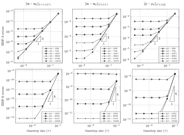
Figure 1: Temporal convergence studies for various mesh sizes. Top: BDF-3, the pair $\mathbb{P}^{3}$–$\mathbb{P}^{3}$ and CIP stabilization. Bottom: BDF-6, the pair $\mathbb{P}^{6}$–$\mathbb{P}^{6}$ and CIP stabilization.

In Figure 1 we plot the discrete analogous of the norms $L^{\infty}(J;L^{2})$, $L^{2}(J;H^{1})$ and $L^{2}(J;L^{2})$ (left to right) for the quantities of interest versus the time step size for various spatial refinements. We test BDF-3 and BDF-6 with the pair $\mathbb{P}^{3}$–$\mathbb{P}^{3}$ and $\mathbb{P}^{6}$–$\mathbb{P}^{6}$ in space, respectively. Note that $\lVert{\boldsymbol{v}}\rVert_{L^{2}(J;V)}=\lVert\nu^{\frac{1}{2}}\nabla{\boldsymbol{v}}\rVert_{L^{2}(J;L^{2})}$ and $\lVert{\boldsymbol{v}}\rVert_{L^{2}(J;Q)}=\lVert\nu^{-\frac{1}{2}}{\boldsymbol{v}}\rVert_{L^{2}(J;L^{2})}$. Both graphs show the predicted optimal-order convergence in time as the error in space becomes smaller and smaller. The error curves flatten out since the spatial error starts dominating for very small time steps. For completeness, we also conducted convergence experiments in space which are summarized in Figure 2 showing that the expected optimal spatial convergence order.

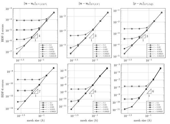
Figure 2: Spatial convergence studies for various time step lengths. Top: BDF-3, the pair $\mathbb{P}^{3}$–$\mathbb{P}^{3}$ and CIP stabilization. Bottom: BDF-6, the pair $\mathbb{P}^{6}$–$\mathbb{P}^{6}$ and CIP stabilization.

8.2 Behavior in the small time step limit

Finally, we briefly revisit the observations and experiments in [12] and illustrate how the initial velocity approximation can affect the error of the pressure approximation for small time steps also in the case of higher-order BDF time stepping methods, cf. Section 7. For initial velocity approximations which are not discretely divergence free, we expect a larger starting error when the small time-step limit is not fulfilled. As in [12], the exact solution is chosen as in (110) with $g(t)=1$ and corresponding right-hand side $f$, boundary and initial data. We compare the error in the pressure after the first computed time step of the BDF scheme, i.e.

$$\tau^{\frac{1}{2}}\lVert p(t_{q})-p_{h}^{q}\rVert_{Q},$$

with two different initial velocity approximation. In Figure 3 the difference between the use of the Ritz projection and the use of a Lagrange interpolant for BDF-3 and BDF-6 is shown (right-hand side column). We verify that the instability already seen in [12] for BDF-1 extends to higher order BDF schemes when the time-step decreases. Also, in the same figure we show how the use of a Ritz projection for the initial data resolves this issue in both cases (left-hand side column).

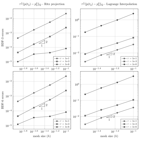
Figure 3: Pressure error studies in the small time-step limit using Ritz projection (left) and Lagrange interpolation (right) for the initial values. Top: BDF-3, the pair $\mathbb{P}^{1}$–$\mathbb{P}^{1}$ and CIP stabilization. Bottom: BDF-6, the pair $\mathbb{P}^{1}$–$\mathbb{P}^{1}$ and CIP stabilization.

Appendix A G-stability for semi-inner product

Lemma 34 is equivalent, as stated in [18, p.65], to require that

(111) $$\sum_{j=0}^{q}\sum_{j=0}^{q}s_{ij}({\boldsymbol{v}}^{i},{\boldsymbol{v}}^{j})\geqslant 0,$$

with

(112) $$S=[s_{ij}]=\begin{bmatrix}\delta_{0}\\ \vdots\\ \delta_{q}\end{bmatrix}\begin{bmatrix}\mu_{0}&\ldots&\mu_{q}\end{bmatrix}+\begin{bmatrix}\mu_{0}\\ \vdots\\ \mu_{q}\end{bmatrix}\begin{bmatrix}\delta_{0}&\ldots&\delta_{q}\end{bmatrix}+\begin{bmatrix}G&\mathbf{0}_{q}\\ \mathbf{0}_{q}^{T}&0\end{bmatrix}+\begin{bmatrix}0&\mathbf{0}_{q}^{T}\\ \mathbf{0}_{q}&G\end{bmatrix},$$

where $\mathbf{0}_{q}=[0,\ldots,0]^{T}$ is the q-th zero vector. One can see that the matrix $S$ is independent from the semi-inner product chosen, but only dependent on the polynomials and thus positive semi-definite by hypothesis. Also, relation (111) holds for any semi-inner product by definition of semi-inner product, thus the Lemma is proven.

Appendix B Estimation of the defect

We want to bound the term $\lVert{\bar{\partial}_{q}}{\boldsymbol{u}}(t_{n})-\partial_{t}{\boldsymbol{u}}(t_{n})-{\bar{\partial}_{q}}{\boldsymbol{e}}_{\pi}^{n}\rVert_{H}^{2}$. By the property of the BDF methods (see [25]) we have that

(113) $${\bar{\partial}_{q}}{\boldsymbol{u}}(t_{n})-\partial_{t}{\boldsymbol{u}}(t_{n})={\bar{\partial}_{q}}R^{n}-R_{t}(t_{n}),$$

where

(114) $$R(t)=\frac{1}{q!}\int_{t_{n-q}}^{t_{n}}(t-s)^{q}\partial_{t}^{(q+1)}{\boldsymbol{u}}(s)\mathop{}\!\textup{d}s,$$

and the following estimate holds, where the Cauchy–Schwarz inequality is used in the last passage

(115) $$\lVert{\bar{\partial}_{q}}{\boldsymbol{u}}(t_{n})-\partial_{t}{\boldsymbol{u}}(t_{n})\rVert_{H}\leqslant C\Bigl{(}\tau^{q-1}\int_{t_{n-q}}^{t_{n}}\lVert\partial_{t}^{(q+1)}{\boldsymbol{u}}(s)\rVert_{H}\mathop{}\!\textup{d}s\Bigr{)}$$

$$=C\left(\tau^{q-2}\int_{t_{n-q}}^{t_{n}}\tau\lVert\partial_{t}^{(q+1)}{\boldsymbol{u}}(s)\rVert_{H}\mathop{}\!\textup{d}s\right)\leqslant C\tau^{q-\frac{1}{2}}\lVert\partial_{t}^{(q+1)}{\boldsymbol{u}}\rVert_{L^{2}((t_{n-q},t_{n});H)}.$$

Moreover, from (115), (99), (18) and using the fact that $\sum_{i=0}^{q}\alpha_{i}=0$ we have

(116) $$\lVert{\bar{\partial}_{q}}{\boldsymbol{e}}_{\pi}^{n}\rVert_{H}=\mathopen{}\left\lVert\frac{1}{\tau}\sum_{i=0}^{q}\Bigl{(}\alpha_{i}{\boldsymbol{e}}_{\pi}^{n-i}-\alpha_{i}{\boldsymbol{e}}_{\pi}^{n-q}\Bigr{)}\mathclose{}\right\rVert_{H}=\mathopen{}\left\lVert\frac{1}{\tau}\sum_{i=0}^{q}\alpha_{i}\int_{t_{n-q}}^{t_{n-1}}\partial_{t}{\boldsymbol{e}}_{\pi}(s)\mathop{}\!\textup{d}s\mathclose{}\right\rVert_{H}$$

$$\leqslant C\tau^{-1}\sum_{i=0}^{q}\mathopen{}\left\lVert\int_{t_{n-q}}^{t_{n-1}}\partial_{t}{\boldsymbol{e}}_{\pi}(s)\mathop{}\!\textup{d}s\mathclose{}\right\rVert_{H}\leqslant C\tau^{-1}\sum_{i=0}^{q}\int_{t_{n-q}}^{t_{n-i}}\mathopen{}\left\lVert\partial_{t}{\boldsymbol{e}}_{\pi}(s)\mathclose{}\right\rVert_{H}\mathop{}\!\textup{d}s$$

$$\leqslant C\tau^{-\frac{1}{2}}\lVert\partial_{t}{\boldsymbol{e}}_{\pi}(s)\rVert_{L^{2}((t_{n-q},t_{n});H)}\leqslant C\tau^{-\frac{1}{2}}h^{r_{\boldsymbol{u}}}\lVert\partial_{t}{\boldsymbol{u}}\rVert_{L^{2}((t_{n-q},t_{n});H^{{\boldsymbol{r}}_{u}}(\Omega))}.$$

Overall

(117) $$\lVert{\bar{\partial}_{q}}{\boldsymbol{u}}(t_{n})-\partial_{t}{\boldsymbol{u}}(t_{n})-{\bar{\partial}_{q}}{\boldsymbol{e}}_{\pi}^{n}\rVert_{H}^{2}\leqslant\lVert{\bar{\partial}_{q}}{\boldsymbol{u}}(t_{n})-\partial_{t}{\boldsymbol{u}}(t_{n})\rVert_{H}^{2}+\lVert{\bar{\partial}_{q}}{\boldsymbol{e}}_{\pi}^{n}\rVert_{H}^{2}$$

$$\leqslant C\Bigl{(}\tau^{2q-1}\lVert\partial_{t}^{(q+1)}{\boldsymbol{u}}\rVert_{L^{2}((t_{n-q},t_{n});H)}^{2}+\tau^{-1}h^{2r_{\boldsymbol{u}}}\lVert\partial_{t}{\boldsymbol{u}}\rVert_{L^{2}((t_{n-q},t_{n});H^{r_{\boldsymbol{u}}}(\Omega))}^{2}\Bigr{)}.$$

References

• [1] N. Ahmed, S. Becher, and G. Matthies, Higher-order discontinuous Galerkin time stepping and local projection stabilization techniques for the transient Stokes problem, Computer Methods in Applied Mechanics and Engineering, 313 (2017), pp. 28–52, https://doi.org/10.1016/j.cma.2016.09.026.
• [2] G. Akrivis, M. Chen, F. Yu, and Z. Zhou, The energy technique for the six-step BDF method, SIAM J. Numer. Anal., 59 (2021), pp. 2449–2472, https://doi.org/10.1137/21M1392656, https://doi.org/10.1137/21M1392656.
• [3] G. Akrivis, M. Feischl, B. Kovács, and C. Lubich, Higher-order linearly implicit full discretization of the Landau–Lifshitz–Gilbert equation, Mathematics of Computation, 90 (2021), pp. 995–1038, https://doi.org/10.1090/mcom/3597.
• [4] G. Akrivis and E. Katsoprinakis, Backward difference formulae: New multipliers and stability properties for parabolic equations, Mathematics of Computation, 85 (2015), pp. 2195–2216, https://doi.org/10.1090/mcom3055.
• [5] G. Akrivis and B. Li, Maximum norm analysis of implicit–explicit backward difference formulae for nonlinear parabolic equations, IMA Journal of Numerical Analysis, 38 (2017), pp. 75–101, https://doi.org/10.1093/imanum/drx008.
• [6] G. Akrivis, B. Li, and C. Lubich, Combining maximal regularity and energy estimates for time discretizations of quasilinear parabolic equations, Mathematics of Computation, 86 (2017), pp. 1527–1552, https://doi.org/10.1090/mcom/3228.
• [7] G. Akrivis and C. Lubich, Fully implicit, linearly implicit and implicit–explicit backward difference formulae for quasi-linear parabolic equations, Numerische Mathematik, 131 (2015), pp. 713–735, https://doi.org/10.1007/s00211-015-0702-0.
• [8] R. Becker and M. Braack, A finite element pressure gradient stabilization for the Stokes equations based on local projections, Calcolo, 38 (2001), pp. 173–199, https://doi.org/10.1007/s10092-001-8180-4.
• [9] N. Behringer, B. Vexler, and D. Leykekhman, Fully discrete best-approximation-type estimates in $L^{\infty}(I;L^{2}(\Omega)^{d})$ for finite element discretizations of the transient Stokes equations, IMA Journal of Numerical Analysis, 43 (2022), pp. 852–880, https://doi.org/10.1093/imanum/drac009.
• [10] F. Brezzi and J. Pitkäranta, On the stabilization of finite element approximations of the Stokes equations, in Efficient Solutions of Elliptic Systems, ViewegTeubner Verlag, 1984, pp. 11–19, https://doi.org/10.1007/978-3-663-14169-3_2.
• [11] E. Burman and M. A. Fernández, Continuous interior penalty finite element method for the time-dependent Navier–Stokes equations: space discretization and convergence, Numerische Mathematik, 107 (2007), pp. 39–77, https://doi.org/10.1007/s00211-007-0070-5.
• [12] E. Burman and M. A. Fernández, Galerkin finite element methods with symmetric pressure stabilization for the transient Stokes equations: Stability and convergence analysis, SIAM Journal on Numerical Analysis, 47 (2009), pp. 409–439, https://doi.org/10.1137/070707403.
• [13] E. Burman and M. A. Fernández, Analysis of the PSPG method for the transient Stokes’ problem, Computer Methods in Applied Mechanics and Engineering, 200 (2011), pp. 2882–2890, https://doi.org/10.1016/j.cma.2011.05.001.
• [14] E. Burman and P. Hansbo, Edge stabilization for the generalized Stokes problem: A continuous interior penalty method, Comput. Methods Appl. Mech. Engrg., 195 (2006), pp. 2393–2410, https://doi.org/10/cgbc89.
• [15] E. Burman and P. Hansbo, Edge stabilization for the generalized Stokes problem: A continuous interior penalty method, Computer Methods in Applied Mechanics and Engineering, 195 (2006), pp. 2393–2410, https://doi.org/10.1016/j.cma.2005.05.009.
• [16] K. Chrysafinos and N. Walkington, Discontinuous Galerkin approximations of the Stokes and Navier-Stokes equations, Math. Comp., 79 (2010), pp. 2135–2167, https://doi.org/10/dgc87n.
• [17] R. Codina and J. Blasco, A finite element formulation for the Stokes problem allowing equal velocity-pressure interpolation, Computer Methods in Applied Mechanics and Engineering, 143 (1997), pp. 373–391, https://doi.org/10.1016/s0045-7825(96)01154-1.
• [18] G. Dahlquist, Error analysis for a class of methods for stiff non-linear initial value problems, in Lecture Notes in Mathematics, Springer Berlin Heidelberg, 1976, pp. 60–72, https://doi.org/10.1007/bfb0080115.
• [19] G. Dahlquist, G-stability is equivalent to A-stability, BIT, 18 (1978), pp. 384–401, https://doi.org/10.1007/bf01932018.
• [20] C. R. Dohrmann and P. B. Bochev, A stabilized finite element method for the Stokes problem based on polynomial pressure projections, International Journal for Numerical Methods in Fluids, 46 (2004), pp. 183–201, https://doi.org/10.1002/fld.752.
• [21] A. Ern and J.-L. Guermond, Finite Elements I, Springer International Publishing, 2021, https://doi.org/10.1007/978-3-030-56341-7.
• [22] A. Ern and J.-L. Guermond, Finite Elements II, Springer International Publishing, 2021, https://doi.org/10.1007/978-3-030-56923-5.
• [23] A. Ern and J.-L. Guermond, Finite Elements III, Springer International Publishing, 2021, https://doi.org/10.1007/978-3-030-57348-5.
• [24] B. García-Archilla, V. John, and J. Novo, Symmetric pressure stabilization for equal-order finite element approximations to the time-dependent Navier–Stokes equations, IMA Journal of Numerical Analysis, 41 (2020), pp. 1093–1129, https://doi.org/10.1093/imanum/draa037.
• [25] E. Hairer and G. Wanner, Solving Ordinary Differential Equations I, Springer Berlin Heidelberg, 1993, https://doi.org/10.1007/978-3-540-78862-1.
• [26] E. Hairer and G. Wanner, Solving Ordinary Differential Equations II, Springer Berlin Heidelberg, 1996, https://doi.org/10.1007/978-3-642-05221-7.
• [27] F. Huang and J. Shen, Stability and error analysis of a class of high-order IMEX schemes for Navier–Stokes equations with periodic boundary conditions, SIAM Journal on Numerical Analysis, 59 (2021), pp. 2926–2954, https://doi.org/10.1137/21m1404144.
• [28] T. Hughes, L. Franca, and M. Balestra, A new finite element formulation for computational fluid dynamics. V. Circumventing the Babuška-Brezzi condition: A stable Petrov-Galerkin formulation of the Stokes problem accommodating equal-order interpolations, Comput. Methods Appl. Mech. Engrg., 59 (1986), pp. 85–99.
• [29] V. John, Finite Element Methods for Incompressible Flow Problems, Springer International Publishing, 2016, https://doi.org/10.1007/978-3-319-45750-5.
• [30] V. John and J. Novo, Analysis of the pressure stabilized Petrov–Galerkin method for the evolutionary Stokes equations avoiding time step restrictions, SIAM Journal on Numerical Analysis, 53 (2015), pp. 1005–1031, https://doi.org/10.1137/130944941.
• [31] B. Kovács, B. Li, and C. Lubich, A convergent evolving finite element algorithm for mean curvature flow of closed surfaces, Numerische Mathematik, 143 (2019), pp. 797–853, https://doi.org/10.1007/s00211-019-01074-2.
• [32] B. Kovács, B. Li, and C. Lubich, A convergent evolving finite element algorithm for Willmore flow of closed surfaces, Numerische Mathematik, 149 (2021), pp. 595–643, https://doi.org/10.1007/s00211-021-01238-z.
• [33] J. Liu, Simple and efficient ALE methods with provable temporal accuracy up to fifth order for the Stokes equations on time varying domains, SIAM Journal on Numerical Analysis, 51 (2013), pp. 743–772, https://doi.org/10.1137/110825996.
• [34] C. Lubich, D. Mansour, and C. Venkataraman, Backward difference time discretization of parabolic differential equations on evolving surfaces, IMA Journal of Numerical Analysis, 33 (2013), pp. 1365–1385, https://doi.org/10.1093/imanum/drs044.
• [35] O. Nevanlinna and W. Liniger, Contractive methods for stiff differential equations part i, BIT, 18 (1978), pp. 457–474, https://doi.org/10.1007/bf01932025.
• [36] O. Nevanlinna and W. Liniger, Contractive methods for stiff differential equations part II, BIT, 19 (1979), pp. 53–72, https://doi.org/10.1007/bf01931222.
• [37] O. Nevanlinna and F. Odeh, Multiplier techniques for linear multistep methods, Numerical Functional Analysis and Optimization, 3 (1981), pp. 377–423, https://doi.org/10.1080/01630568108816097.
• [38] J. Schoeberl, C++11 implementation of finite elements in NGSolve, Vienna University of Technology - Institute for Analysis and Scientific Computing, (2014).
• [39] J. Schöberl, NETGEN an advancing front 2d/3d-mesh generator based on abstract rules, Computing and Visualization in Science, 1 (1997), pp. 41–52, https://doi.org/10.1007/s007910050004.