cuSZ-I: High-Fidelity Error-Bounded Lossy Compression for Scientific Data on GPUs

Jinyang Liu^∙(⋆), Jiannan Tian^∘(⋆), Shixun Wu^∙(⋆), Sheng Di^†, Boyuan Zhang^∘, Yafan Huang^§, Kai Zhao^‡, Guanpeng Li^§, Dingwen Tao^∘, Zizhong Chen^∙, Franck Cappello^† jliu447@ucr.edu, jti1@iu.edu, swu264@ucr.edu, sdi1@anl.gov, bozhan@iu.edu, yafan-huang@uiowa.edu, kzhao@cs.fsu.edu, guanpeng-li@uiowa.edu, ditao@iu.edu, chen@cs.ucr.edu, cappello@mcs.anl.gov ^(⋆)Co-first Authors ^∙University of California, Riverside, Riverside, CA, USA ^∘Indiana University, Bloomington, IN, USA ^†Argonne National Laboratory, Lemont, IL, USA ^§The University of Iowa, Iowa City, IA, USA ^‡Florida State University, Tallahassee, FL, USA

Abstract

Error-bounded lossy compression is a critical technique for significantly reducing scientific data volumes. Compared to CPU-based scientific compressors, GPU-accelerated compressors exhibit substantially higher throughputs, which can thus better adapt to GPU-based scientific simulation applications. However, a critical limitation still lies in all existing GPU-accelerated error-bounded lossy compressors: they suffer from low compression ratios, which strictly restricts their scope of usage. To address this limitation, in this paper, we propose a new design of GPU-accelerated scientific error-bounded lossy compressor, namely cuSZ-I, which has achieved the following contributions: (1) A brand new GPU-customized interpolation-based data prediction method is raised in cuSZ-I for extensively improving the compression ratio and the decompression data quality. (2) The Huffman encoding module in cuSZ-I has been improved for both efficiency and stability. (3) cuSZ-I is the first work to integrate the highly effective NVIDIA bitcomp lossless compression module to maximally boost the compression ratio for GPU-accelerated lossy compressors with nearly negligible speed degradation. In experimental evaluations, with the same magnitude of compression throughput as existing GPU-accelerated compressors, in terms of compression ratio and quality, cuSZ-I outperforms other state-of-the-art GPU-based scientific lossy compressors to a significant extent. It gains compression ratio improvements by up to 500% under the same error bound or PSNR. In several real-world use cases, cuSZ-I also achieves the optimized performance, having the minimized time cost for distributed lossy data transmission tasks and the highest decompression data visualization quality.

I Introduction

Large-scale scientific applications for advanced instruments produce vast data for post hoc analysis every day, creating exascale scientific databases in single or distributed supercomputing clusters. For instance, Hardware/Hybrid Accelerated Cosmology Code (HACC) [1, 2] may produce petabytes of data in hundreds of snapshots when simulating 1 trillion particles. Those extremely large databases raise tough challenges for the utility of those data. To this end, data reduction is becoming an effective method to resolve the big data issue for scientific databases. Although traditional methods of lossless data reduction can guarantee zero information loss, they suffer from limited compression ratios. Specifically, deduplication usually reduces the scientific data size by only 20% to 30% [3], and lossless compression by roughly 2:1 [4].

Over the past years, error-bounded lossy compressors have strived to address the high compression ratio requirements for scientific data: they not only get very high compression ratios (such as a magnitude of multi-hundred) [5, 6, 7, 8], but also perform strict control over the data distortion regarding various modes of user-set error bounds. With the development of computing hardware such as GPUs, modern scientific simulation has started to leverage that hardware, and their data throughput has risen a lot. In an LCLS-II laser [9] X-ray imaging use case, it tops at 250 GB/s [10]; such a kind of rate is far beyond the level that typical CPU-centric compressing systems can handle. To meet the high-throughput-compression need for modern scientific applications, especially for the ones on GPU platforms, several GPU-based error-bounded lossy compressors have been developed, such as cuSZ [11, 12], cuSZx [13], FZ-GPU [14], cuSZp [15], and cuZFP [16]. Those compressors can exhibit very high compression throughputs (from tens to hundreds of Gigabytes per second). Therefore, they can be well applied to more diverse use cases, such as streaming compression of data and fast data transfer between distributed data centers or databases. Nevertheless, to maintain the high throughputs, their data compression and reconstruction algorithms are quite sub-optimal in terms of data reduction rates, so they suffer from low compression ratio and fidelity, respectively. For example, as the GPU-based error-bound lossy compressor with the highest compression ratio among existing GPU-accelerated compressors, cuSZ can obtain a compression ratio that is only 10% to 30% of the CPU-based compressor SZ3 under the same PSNR. Thus, the requirement of high-fidelity error-bounded lossy compression for scientific data on GPU platforms has not yet been fulfilled by existing works.

Taking the characteristics of existing error-bounded lossy compressors into account, we would like to take advantage of both CPU-based and GPU-based compressors meanwhile avoiding their limitations. Specifically, we are motivated to develop a GPU-based error-bounded lossy compressor with relatively high compression throughput (far over CPU-based ones) and quite acceptable compression ratios (quite improved over GPU-based ones). Having succeeded in overcoming the challenge of designing a GPU-customized compression pipeline with both high compression efficiency and fidelity, in this paper, we propose a GPU-accelerated error-bounded lossy compressor, namely cuSZ-I. Specifically, cuSZ-I integrates a delicately customized and highly parallelized interpolation-based data predictor and introduces an improved Huffman encoding module together with the NVIDIA bitcomp module for high-end lossless postprocessing. cuSZ-I preserves a high compression throughput within the same magnitude as existing GPU-accelerated compressors and profoundly prevails over all other GPU-accelerated compressors in terms of compression ratio and distortion. To our best knowledge, cuSZ-I is the first and the only high-fidelity GPU-accelerated scientific error-bounded lossy compressor, which fills the large gap between the compression fidelity of CPU-based and GPU-based scientific lossy compressors. We summarize our contributions as follows:

• Motivated by the SZ3 and QoZ interpolation design, we develop a GPU-customized interpolation-based data predictor G-Interp with highly parallelized efficient interpolation, which can present excellent data prediction accuracy, thus leading to a high overall compression ratio.

• We design and implement a highly lightweight interpolation auto-tuning kernel for GPU interpolation to optimize both performance and compression quality of cuSZ-I.

• We improve the implementation of GPU-based Huffman encoding and import a new lossless module NVIDIA Bitcomp to further reduce its encoding redundancy.

• In terms of experimental evaluation, cuSZ-I improves compression ratio over other state-of-the-art GPU-based scientific lossy compressors extremely, by up to about 500% under the same error bound or PSNR. Meanwhile, it preserves a compression throughput of the same magnitude as other compressors, such as cuSZ and cuSZp.

The rest of this paper is arranged as follows: §II introduces related works. §III provides the background and motivation for our research. §IV demonstrates the framework of cuSZ-I. The design of cuSZ-I interpolation-based predictor: G-Interp is illustrated in detail in §V, and the new design of cuSZ-I lossless postprocessing modules is proposed in §VI. In section VII, the evaluation results are presented and analyzed. Finally, §VIII concludes our work and discusses future work.

II Related Work

Data compression for scientific data has been studied for years to address the issue of the storage burden and I/O overheads. The compression techniques are in two classes: lossless and lossy. Compared to lossless compression, lossy compression can provide a much higher compression ratio at the cost of accuracy loss. However, scientific computing practice often requires the error to be quantitatively determined for accurate post-analysis so that commodity lossy compressors, such as JPEG [17] or MPEG [18], fall short in strict error control.

Recently, many error-bounded lossy compressors for scientific data have been developed, such as SZ [19, 6], ZFP [20], QoZ [7], SPERR [8], TTHRESH [21], and several AI-assisted works [22, 23, 24]. Unlike the mentioned commodity lossy compressors for images and video, these compressors extend their usability beyond vision perception by allowing users to strictly control the accuracy loss in data reconstruction and post-analysis in a wide range of domains.

Considering the increasing popularity of heterogenous HPC systems and applications, GPU-accelerated scientific lossy compressors have been proposed to deliver orders of magnitude higher throughputs than CPU compressors. Specifically, cuZFP [16], the CUDA implementation of transform-based ZFP, allows the user to specify the desired bitrate; cuZFP features. Also, prediction-based GPU compressors have been proposed, including cuSZ, cuSZx [13], FZ-GPU [14], and cuSZp [15]. While sharing the error-boundness in the reconstructed data, these prediction-based compressors can fit into different use scenarios, as detailed below. 1) cuSZ [11, 12] (the first GPU-accelerated SZ framework) features fully parallelized prediction-quantization with outlier compacted and coarse-grained Huffman coding that encodes multibyte quantization codes using bits inverse to their frequencies; it is also the basis of this work. 2) cuSZx [13] features a monolithic design to deliver extremely high throughput at the cost of lower data quality and compression ratio. 3) FZ-GPU features an alternative compression pipeline by replacing the entire lossless encoding stage with bit-shuffle and dictionary encoding, aiming to deliver higher throughput than the default cuSZ. 4) cuSZp [15] modifies cuSZ by fusing prediction-quantization and 1D blockwise encoding subroutine into a monolithic GPU kernel, practically achieving high end-to-end throughput. The limitations of those GPU-accelerated compressors are as follows: 1) all the aforementioned GPU-based compressors focus on high throughputs at the cost of suboptimal compression ratios. Specifically, They tend to compromise the data quality in the use scenario with high kernel throughput or low end-to-end system turnaround time. 2) cuSZ, FZ-GPU, and cuSZp feature Lorenzo prediction, whose data quality is ceiled, as described in [19].

III Background and Research Motivation

In this section, we introduce and detail our research background. First, we demonstrate cuSZ (the CUDA version of SZ) [11, 12] as it is a typical representative of GPU-accelerated scientific error-bounded lossy compressors and is also the fundamental of cuSZ-I. Next, we specify our research motivation by analyzing the characteristics and limitations of cuSZ with experimental results, then set up our research target.

III-A cuSZ Framework

The compression pipeline of cuSZ involves nine steps to adapt to the GPU architecture. Specifically, Step-1 splits the whole dataset into multiple blocks, each of which will be compressed independently. This design favors coarse-grained decompression. Upon splitting blocks, cuSZ’s compression adopts a dual-quantization scheme (including prequantization, prediction, and post-quantization), which can entirely remove the data dependency for the Lorenzo prediction. Then, Step-5 adopts parallel histogramming to compute the quant-codes frequencies. Step-6 builds a canonical Huffman codebook [11] based on the histogram/frequency vector. Step-7 performs the Huffman encoding over the quant-codes. Step-8 concatenates all the Huffman codes (called deflating) on GPUs, which feeds a dictionary encoder (Zstd [25]) for further compression on CPUs in Step-9. The decompression is a reversion of the compression. We refer readers to the cuSZ paper [11] for more details.

For compression, Step-6 and -9 are the main bottlenecks because Step-6 has to be executed sequentially with a single GPU thread and designing an efficient multi-thread GPU algorithm for dictionary encoding is non-trivial.

The first step (i.e., the reversed dual-quantization) is the main bottleneck for decompression since the decompression cannot use the massive parallelism as the pre-quantization step does, and the data values must be reconstructed one by one, according to the Lorenzo predictor. To address this issue, cuSZ adopts a coarse-grained parallel method instead, letting one GPU thread handle one independent data block in parallel. However, such a design suffers from non-coalesced memory and warp divergence on GPUs, leading to low performance. In addition to Step-1, Step-9 is another significant bottleneck because the dictionary decoding is also very hard to parallelize on GPUs because of its intrinsic data dependency.

III-B Research Motivations

In this part, we discuss several key limitations of cuSZ, then propose our design target of cuSZ-I to address those issues.

III-B1 Limitation of cuSZ in data prediction quality

The first limitation of cuSZ is that the data prediction quality of the Lorenzo predictor in cuSZ is sub-optimal in various cases. Core evidence is that cuSZ ’s compression ratios are far lower than specific prediction-based compressors on CPU such as SZ3 [19, 6]. Therefore, we would like to learn from the advanced predictor design of high-ratio CPU data compressors and propose a GPU-customized high-accuracy data predictor for error-bounded lossy compression on GPUs.

III-B2 Limitation of cuSZ in lossless post-processing

Another critical limitation of cuSZ is that, since its lossless post-processing module is only the Huffman encoding, mapping each data element to at least 1 bit, the compression bit rate of cuSZ is always higher than 1. More importantly, the compressed data of cuSZ still has high redundancy in broad cases. Therefore, we need to address this issue by designing or employing new lossless post-processing techniques.

III-B3 Design goals of cuSZ-I

Overall, for cuSZ-I, we endeavor to significantly boost the compression fidelity of cuSZ by developing a series of optimization techniques to address the above issues. Our development plan for cuSZ-I contains and is not limited to 1) leveraging a more effective data prediction scheme for better compression quality. 2) Integrating high-performance lossless modules in the compression pipeline for better compression ratios. One core challenge is that the existing high-accuracy data predictor design, including SZ3 and QoZ interpolators, are all implemented on CPU, lacking parallelizability and featuring poor throughputs if directly transferred to GPUs. In the following sections, we will present how we overcame this challenge by proposing a novel platform-aware design of data predictor to optimize the prediction throughput on GPUs.

IV cuSZ-I Design Overview

Figure 1: Proposed cuSZ-I compression framework. The shading indicates the key difference of our work, cuSZ-I, from cuSZ, which result in a significant improvement in both data reconstruction fidelity and compression ratio.

In this section, we present the general design overview of cuSZ-I. First, the overall compression framework of cuSZ-I is featured in Fig. 1. Like cuSZ and many other GPU-accelerated compressors, cuSZ-I is also a prediction-based error-bounded lossy compressor with several key modules, including data prediction, error quantization, and lossless encoding. In the compression pipeline, cuSZ-I attempts to recover the input data from scratch with a data predictor, and the prediction errors are quantized and recorded. The quantized errors are further encoded and stored to be used in the decompression process. The core innovations in cuSZ-I are:

• Instead of low-accuracy Lorenzo data predictor [26, 5], cuSZ-I introduces a GPU-customized interpolation-based data predictor, presenting high data prediction accuracy and parallelization efficiency.

• To jointly optimize the quality and performance of the interpolation-based data predictor, a lightweight profiling-based interpolation auto-tuning kernel is integrated.

• To maximize the compression ratio and throughput of predicted error quant-codes, the Histograming phase of the Huffman encoding phase is optimized, and a new lossless module, NVIDIA Bitcomp is introduced.

• For maximally boosting the compression ratio of cuSZ-I with minor speed degradation, the NVIDIA bitcomp lossless compressor is appended to the Huffman Encoding module as a lossless post-processing module.

In the next sections, those innovative design details, which have substantially optimized the compression of cuSZ-I, will be comprehensively demonstrated.

V cuSZ-I Interpolation-based Data Predictor

Based on CPU interpolation-based data predictor design [19, 7, 27], cuSZ-I introduces a new interpolation-based prediction scheme (named G-Interp) for GPU platforms featuring hardware-software codesign. The new scheme consists of a spline interpolative predictor utilizing anchor points and an auto-tuning strategy. In most use scenarios, the new interpolative predictor shows advantages over the Lorenzo predictor in terms of prediction accuracy and compression ratio.

V-A Basic Design Concept of G-Interp

Fig. 2 demonstrates the basic design concept of G-Interp by a 3D example. Instead of directly transferring the accurate but slow existing CPU-based interpolation data predictors [19, 7, 27] to GPU platforms, G-Interp has been re-designed according to the characteristics of the hardware to maximize its data parallelism and computing parallelism, meanwhile preserving enough data prediction accuracy. To this end, we first partition the input data into relatively small chunks and eliminate the data dependencies across them. In the example, the input 3D data array is partitioned into $8\times 8\times 8$ data chunks (or $16\times 16$ for 2D chunks/512 for 1D chunks). Next, to avoid data and computational dependencies across the chunks, the interpolation operations need to be confined within a short range. Inspired by [7], we introduced anchor points in G-Interp that are losslessly stored so that all interpolations can be bounded in the range of 2 adjacent anchor points (i.e., within one single data chunk). In each data chunk, one vertice point is assigned as an anchor point (red points in Fig. 2), and seven (7) other anchor points (on the rest vertices) are borrowed from the surrounding chunks, as indicated in Fig. 2-(1). Afterward, the interpolation within each data chunk is entirely independent of other chunks, so can be performed in parallel. In the 3D input data array, approximately 1 of 512 elements becomes an anchor point, making up at most 1/512 overhead to save the anchor points.

Having set up the partitioned data chunks and anchor points, as is shown in Fig. 2-(3-4), the interpolation-based data predictions in each data chunk are performed in parallel. Like in existing works [19, 7], the interpolations are performed level by level, from a large stride to smaller ones (from 4 to 2 and 1 for G-Interp), and each chunk is expanded from $1\times 1\times 1$ to $2\times 2\times 2$, $4\times 4\times 4$, lastly $8\times 8\times 8$. In each level, the interpolations are performed subsequently along each dimension. Moreover, within each data chunk, the interpolations on the same level and along the same dimension are also performed in parallel since they have no dependencies. Later, we will feature important details of this process, including the interpolation splines, error bounds, and the order of interpolation direction.

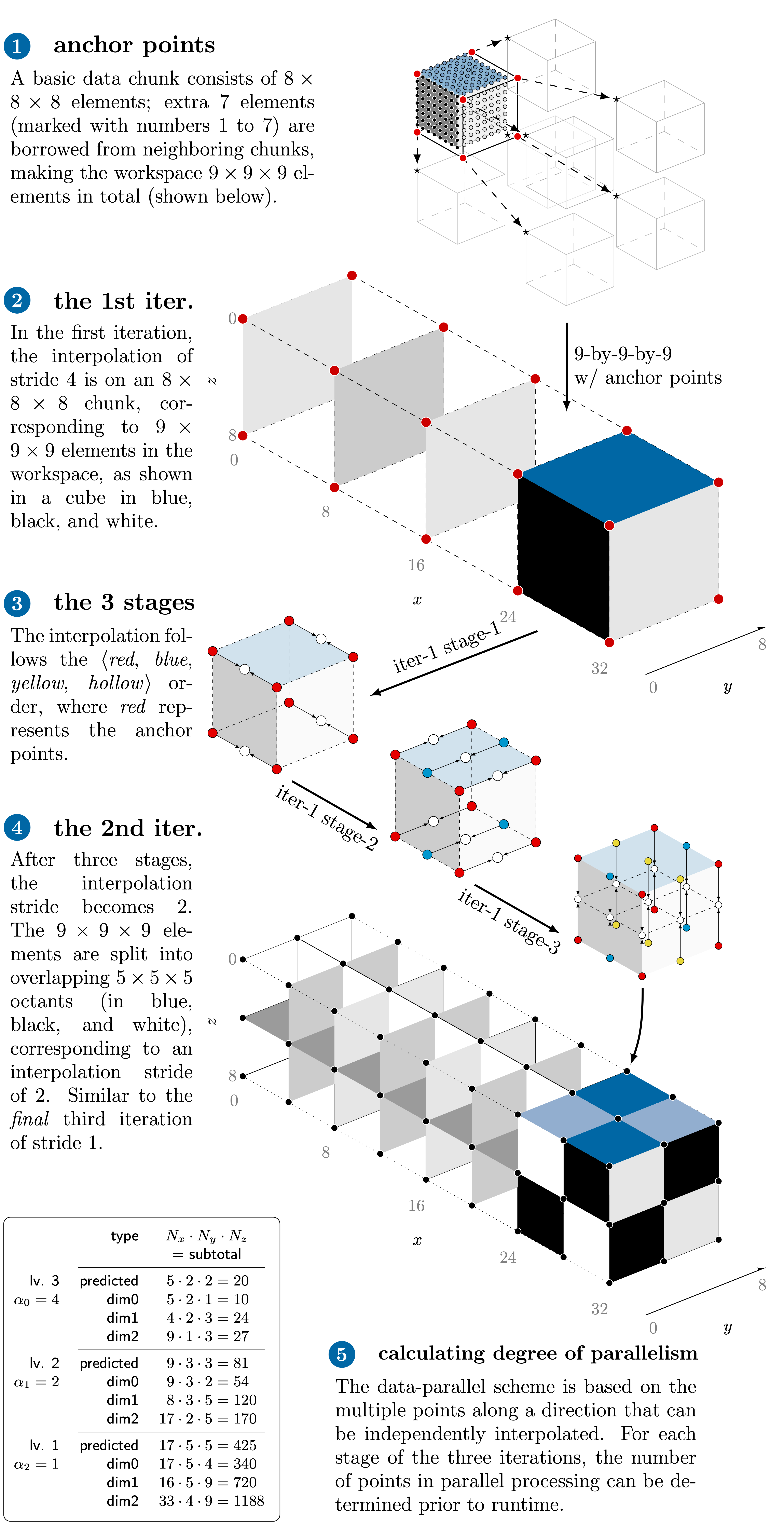
Figure 2: Anatomy of data parallelism found in G-Interp.

V-B Interpolation Configurations of G-Interp

V-B1 Interpolation splines

As described in Fig. 2, on a multi-dimensional data grid, G-Interp performs the interpolations with 1D spline functions, and the interpolations are executed along different dimensions. For the specific 1D spline functions, Fig. 3 presents an example showing 1D data slices. For each interpolation (to predict the data point $x_{n}$ with a predicted value $p_{n}$), depending on the number of available neighbor points, there are four circumstances:

• 4 neighbors available: The cubic spline interpolation with $x_{n-3}$, $x_{n-1}$, $x_{n+1}$, and $x_{n+3}$ is computed to predict $x_{n}$;

• 3 neighbors available: The quadratic spline interpolation with $x_{n-3}$, $x_{n-1}$, and $x_{n+1}$ (or $x_{n-1}$, $x_{n+1}$, and $x_{n+3}$) is computed to predict $x_{n}$;

• 2 neighbors available: The linear spline interpolation with $x_{n-1}$ and $x_{n+1}$ is computed to predict $x_{n}$;

• 1 neighbour available: $x_{n-1}$ serves as a prediction of $x_{n}$.

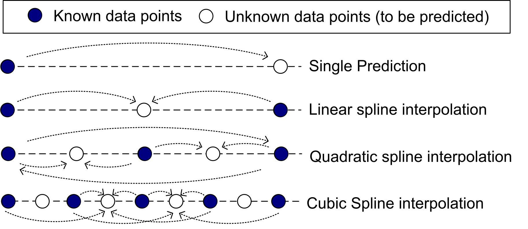
Figure 3: Interpolation splines.

Fig. 4 shows another example of the interpolations on a 9x9 2D grid with an anchor stride of 8. The predicted data points with different interpolation splines are marked with their corresponding shapes. For the conciseness of the paper, we list each spline function in G-Interp as follows, which is deducted by the analyses in [19] and [27]:

• Linear Spline:

  $$\textstyle p_{n}=\frac{1}{2}x_{n-1}+\frac{1}{2}x_{n+1}$$

• Quadratic Spline:

  $$\begin{split}p_{n}&=\textstyle-\frac{1}{8}x_{n-3}+\frac{6}{8}x_{n-1}+\frac{3}{8}x_{n+1}\\ \text{or\ \ }p_{n}&=\textstyle\phantom{-}\frac{3}{8}x_{n-1}+\frac{6}{8}x_{n+1}-\frac{1}{8}x_{n+3}\end{split}$$

• Cubic Spline (not-a-knot):

  $$\textstyle p_{n}=-\frac{1}{16}x_{n-3}+\frac{9}{16}x_{n-1}+\frac{9}{16}x_{n+1}-\frac{1}{16}x_{n+3}$$

• Cubic Spline (natural):

  $$\textstyle p_{n}=-\frac{3}{40}x_{n-3}+\frac{23}{40}x_{n-1}+\frac{23}{40}x_{n+1}-\frac{3}{40}x_{n+3}$$

Figure 4: Interpolations on a 2D slice (interpolations are performed first along dim0 and then along dim1).

It is worth noticing that there are 2 different cubic splines serve the same circumstance because each can outperform the other on different datasets. An auto-tuning model of G-Interp will make the selection of cubic splines during each compression task. This process will be detailed in §V-C2.

V-B2 Level-wise interpolation error bound

An important feature of interpolation-based prediction is that the data prediction and the error control process are performed synchronously. For each to-be-predicted data point, G-Interp quantizes the error of its interpolation-based prediction and fixes the prediction value with an offset of the quantized error. The fixed prediction will serve as the decompression output of it and will also be used for predicting subsequent to-be-predicted data points. Therefore, the prediction quality on early interpolations will impact those predicted later. [7] verified that, for this prediction paradigm, applying lower error bounds on higher interpolation levels (with larger interpolation strides) than lower levels may significantly improve the compression distortion with little compression ratio degradation, or in certain cases, it can even improve both compression ratio and distortion. Thus, similarly with [7] and [27], G-Interp reduces the error bounds for high-level interpolations according to Eq. 1:

$$e_{\ell}=\frac{e}{\alpha^{\ell-1}}\ (\alpha\geq 1)$$ (1)

In Eq. 1, $e$ is the global error bound, $\ell$ is the interpolation level (level 1 is stride-1 interpolation, level 2 is stride-2 interpolation, and so on), and $e_{\ell}$ is the error bound on level $\ell$. $\alpha$ is a parameter of error-bound reduction. In §V-C2, we will discuss determining the specific value of $\alpha$.

V-C Profiling-based Auto-tuning of G-Interp Interpolations

Because the prediction accuracy of interpolation-based data predictors is highly sensitive to their configurations [7], auto-tuning modules are often leveraged jointly with the interpolation-based predictors for preserving the data prediction accuracy[19, 7, 28, 27]. [19], [7], and [27] have proposed diverse effective auto-tuning strategies. However, those CPU-based auto-tuning strategies can not be simply transferred to GPU platforms because the relative computational overhead of those strategies will be much higher (so unacceptable) on GPUs. Considering the hardware characteristics of GPUs, we design a new novel lightweight profiling-and-auto-tuning kernel for G-Interp, which has only a trivial computational overhead. This auto-tuning kernel comprises two functionalities: data-profiling and interpolation configuration auto-tuning.

V-C1 Data-profiling

We profile the input data array in 2 steps. First, we compute its value range to acquire both the absolute error bound and the value-range-based relative error bound (the absolute error bound divided by the value range). Second, from the data array, 64 data points are uniformly sampled (e.g., from a 4x4x4 sub-grid for 3D data). For each sampled data point, we perform two spline interpolation tests with 2 cubic splines along each dimension (e.g., for 3D data, there are a total of 2$\times$3=6 interpolation tests). On all sampled data points, the profiling kernel accumulates the interpolation prediction errors separately for each interpolation spline/dimension.

V-C2 Interpolation auto-tuning

With the profiling information, G-Interp determines the interpolation configurations by the following strategy. First, G-Interp computes the error-bound reduction factor $\alpha$ by a piecewise linear function of the value-range-based relative error bound $\epsilon$:

$$\alpha=A(\epsilon)=\begin{cases}2&{10^{-1}\leq\epsilon}\\ 1.75+0.25\cdot\frac{\epsilon-10^{-2}}{10^{-1}-10^{-2}}&{10^{-2}\leq\epsilon<10^{-1}}\\ 1.5+0.25\cdot\frac{\epsilon-10^{-3}}{10^{-2}-10^{-3}}&{10^{-3}\leq\epsilon<10^{-2}}\\ 1.25+0.25\cdot\frac{\epsilon-10^{-4}}{10^{-3}-10^{-4}}&{10^{-4}\leq\epsilon<10^{-3}}\\ 1+0.25\cdot\frac{\epsilon-10^{-5}}{10^{-4}-10^{-5}}&{10^{-5}\leq\epsilon<10^{-4}}\\ 1&{\epsilon\leq 10^{-5}}\end{cases}$$ (2)

Eq. 2 is established for two reasons. On one hand, our and [7]’s observations are that the optimized value of $\alpha$ is relevant to $\epsilon$ and should decrease with the decreasing of $\epsilon$. On the other hand, the user requirements for compression tasks under different error bounds may vary. When the error bound is large, the compression ratio is high enough. Still, the compression quality is relatively low, so we would like to improve the decompression data quality with acceptable compression ratio loss by using large $\alpha$. In contrast, the decompression quality is good enough when the error bound is small, but the compression ratio is limited. Therefore, we would like to apply a small $\alpha$ to maximize the compression ratio. To reduce computational cost, we apply this empirical but effective calculation instead of a more precise optimization for $\alpha$.

Next, G-Interp evaluates the cubic splines and the smoothness of dimensions via the profiled interpolation errors. For each dimension, the cubic spline with the lower error will be applied. Moreover, on each level, the interpolation will start from the most unsmooth dimension (the largest profiled interpolation error) and end in the smoothest dimension (the smallest profiled interpolation error). The reason for this design is explained in [19]: The earlier processed dimension will have fewer interpolations performed along it, and vice versa. By performing more interpolations along smoother dimensions, the overall data prediction accuracy can be well optimized.

V-D Parallelizing G-Interp on GPU

After discussing G-Interp ’s design concepts, it now comes to how we create an efficient design of it on GPU platforms, maximally taking advantage of the modern GPU architecture. The challenges are as follows: 1) the algorithm and data access pattern determine that a portion of data loading and storing are non-coalescing ; 2) the iterative nature of the algorithm determines data dependency in traversal in each dimension and loop iteration at coarse-to-fine interpolation levels. Our solutions to meet the challenges are stated below.

First, for each GPU thread block, we need to exploit its data capacity as much as possible to optimize the thread usage. Therefore, the data chuking is arranged as illustrated in Fig. 2 (2-4). A basic block consists of $8\times 8\times 8$ elements (featured in §V-A), and the data chunk for each GPU thread consists of 4 basic blocks, building up a $32\times 8\times 8$ chunk (Fig. 2(2)). This style of loading data aims to minimize the DRAM transaction, followed by another load of borrowed anchor points from neighbor blocks before interpolation. Fig. 2(2) shows the data chunk for the first level of interpolation (the interpolation stride is $\alpha_{0}=4$). Fig. 2(4) is the further-expanded block after interpolation with stride $\alpha_{1}=2$.

Next, for each GPU thread block, its interpolations are fully within a $33\times 9\times 9$ data block, i.e., the $32\times 8\times 8$ input data chunk with borrowed anchor points, as shown in Fig. 2 (2). The interpolations are performed as described in §V-A, but now more neighbor points can be available as 4 basic blocks can share their data. For each level of interpolation, Fig.2 (5) lists the numbers of the interpolated points along each dimension (suppose the interpolations are performed from Dim0 with length 9 to Dim2 with length 33). In the level 1 interpolation, the number of interpolated points surpasses the thread number limits of each thread block. Thus we dynamically assign the number of data points for an active thread.

The full implementation is illustrated in Algorithm 1. We modularized the interpolation kernel with an emphasis on the expressiveness of the code structure. Specifically, we have 1) the basic interpolative prediction on each data point (PerDataPointPrediction), 2) the wrapper of prediction-quantization and its reverse for compression and decompression (PredQuantWarpper), respectively, 3) the stage of interpolation that dynamically states the data-thread parallelism relationship given distance $\alpha$ (Stage), and 4) the high-level view of three-stage 3D interpolation for an iteration (i.e., given $\alpha$).

Algorithm 1: G-Interp Implementation. For simplicity, auto-tuning and DRAM traffic are excluded.

1* notation: original data element/value $d$, predicted value $p$, prediction error $e$, quant-code $q$, error bound $eb$, radius $r$

2

3** we refer reader to Tao et al. 2017 for the detailed CompressQuant and DecompressQuant (quantization for compression and decompresison, respectively) algorithm description.

4

5*** Cubic fuction is defined according to out-of-line formula.

6

7procedure PerDataPointPredict<sym C>(volatile $b$, $x$, $y$, $z$, $\alpha$)

8    if constexpr (C $\equiv$ X-dir.) return Cubic($b_{y,z}$; $x\pm\alpha$)

9    if constexpr (C $\equiv$ Y-dir.) return Cubic($b_{x,z}$; $y\pm\alpha$)

10    if constexpr (C $\equiv$ Z-dir.) return Cubic($b_{x,y}$; $z\pm\alpha$)

11end procedure

12

13procedure PredQuantWrapper<sym CATEGORY, ...>(volatile $shm\{data,quant\}$, $x$, $y$, $z$, $\alpha$)

14    reference $d\leftarrow shm.data_{z,y,x}$

15    reference $q\leftarrow shm.quant_{z,y,x}$; declare $p$

16    if ok $\leftarrow$ BoundaryCheck($x$, $y$, $z$) then

17       $p\leftarrow$ PerDataPointPredict<CATEGORY>($b$, $x$, $y$, $z$, $\alpha$)

18       if constexpr (COMPRESS) CompressPredQuant($d$, $p$, $q$)

19       if constexpr (DECOMPRESS) DecompressPredQuant($d$, $p$, $q$)

20    end if

21end procedure

22

23procedure Stage<class Map>(..., Map map)

24    if constexpr COARSENING then $\triangleright$ # data element $\geq$ # thread

25       repeat$\triangleright$ $\tau$: thread id indirection

26          $\tau\leftarrow$ BlockDimStride(threadIdx.x)

27          $x,y,z\leftarrow$ map($\tau$, $\alpha$); PredQuantWrapper(..., $x$, $y$, $z$, $\alpha$)

28       until finish iterating

29    else

30       $x,y,z\leftarrow$ map(threadIdx.x, $\alpha$); PredQuantWrapper(..., $x$, $y$, $z$, $\alpha$)

31    end if

32end procedure

33

34procedure InterpolateIter(volatile $shm\{data,quant\}$)

35    for $\alpha\leftarrow\{4,2,1\}$, with predefined parallelism config. do

36       Stage<DIM0>(...); Stage<DIM1>(...); Stage<DIM2>(...)

37    end for

38end procedure

V-E Advantages of G-Interp: An Quantitative Analysis of Comparison between G-Interp and Lorenzo in cuSZ

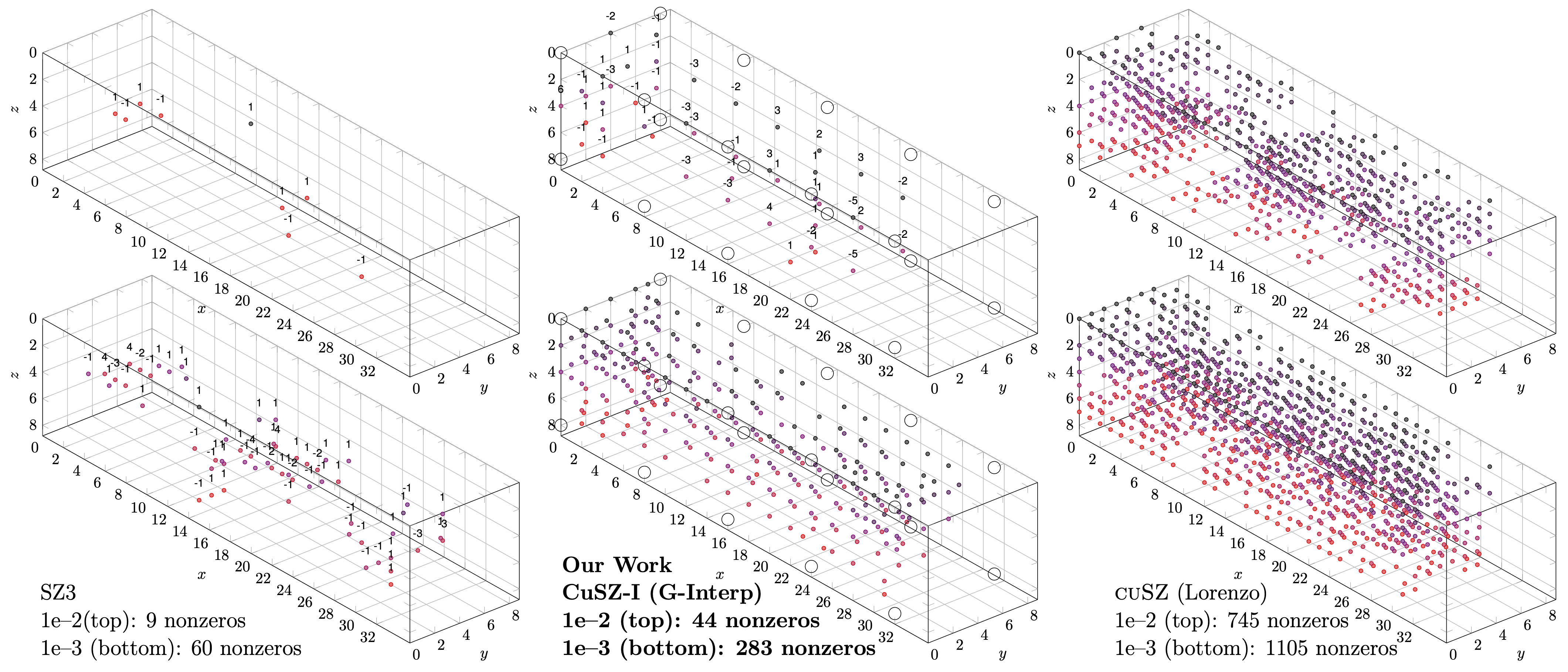
Figure 5: Count comparison of nonzero quant-code among CPU SZ3, GPU G-Interp, and GPU Lorenzo with two relative-to-value-range error bounds on Pressure field of Miranda dataset. Small blocks within the 33-by-9-by-9 bounding box indicate the presence of the nonzeros

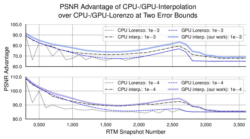
Figure 6: The PSNR advantage of spline interpolation over Lorenzo prediction on two error bounds. The snapshots are selected at every 100 intervals in the dataset of 3700. Some initial snapshots are excluded, as they correspond to the simulation’s initialization phase.

In many use scenarios, G-Interp shows advantages over the cuSZ Lorenzo predictor. The improvement can be summarized into two aspects.

First, with better data prediction capability, G-Interp generally produces more minor predicting errors. Since those errors will be quantized to a collection of integers, smaller errors will definitely lead to a more concentrated distribution of quantization bins and a higher compression ratio after the Huffman Encoding process. We have a case study as shown in Fig. 5, which compares the quantized prediction errors of cuSZ-Lorenzo, G-Interp, and CPU-interpolation SZ3 (as a benchmark) when applied on the pressure field of the Miranda dataset [29]. In the figure, the non-zero quant-codes (i.e., the prediction error is larger than $eb$) are marked, with color changing according to the amplitude of the quant-code. Under the same error bounds, the G-Interp design results in much less non-zero quant-codes than cuSZ-Lorenzo predictor and smaller in the amplitude, achieving closer outcomes with the CPU-based SZ3.

Next, because G-Interp exhibits significantly better data prediction accuracy than cuSZ-Lorenzo, its data reconstruction fidelity is also substantially improved over the Lorenzo predictor. In Fig. 6, we propose the comparison between decompression PSNR of G-Interp and cuSZ-Lorenzo (under the same error bound, both CPU-based and GPU-based) on 37 snapshots of the RTM dataset (sample 1 snapshot from every 100 time steps). We find that G-Interp is constantly better than GPU-Lorenzo in terms of PSNR under all error bounds, gaining 2.5 $\sim$ 10 dB of PSNR improvements. Moreover, attributed to the anchor point design, the PSNR from G-Interp even outperforms the CPU version of interpolation (implemented in SZ3 [19]), although its compression ratios are still lower than SZ3.

As such, the prediction of G-Interp overperforms the original Lorenzo predictor of cuSZ to a great extent. Admittedly, One key shortcoming of G-Interp compared to the Lorenzo predictor is that it has higher computational costs and lower prediction throughputs. In §VII we will show that, in various cases when the compression ratio is mostly concerned with saving storage space or data transmission time, the trade-off between fidelity and speed made in cuSZ-I is essential.

VI Improving cuSZ-I Lossless Modules

In this section, we detail several important improvements we have made to the cuSZ-I lossless post-processing module, which performs a key role in optimizing the compression ratio of G-Interp-predicted quant-codes.

VI-A Tweaking Existing Huffman Coding

Adapted from the previous practice [11], Huffman encoding remains in the cuSZ-I pipeline, with several tweaks adjusted. Prior to building the Huffman codebook, a histogram that presents the frequencies of the quantization codes is needed. Since the quantization codes are highly centralized at zero thanks to the accurate prediction from G-Interp,Unlike the general-purpose histogramming practice, we allocate a thread-private buffer of small size $k$ to cache the count of the center top-$k$ quantization codes. This significantly decreases the transaction between the threads’ register file and shared memory buffer, which is relatively slow. Moreover, according to [30], only when the Huffman tree is large enough can we exploit the parallelism to build the Huffman tree on GPUs. Given the dominance of the top symbols, being latency-dominated, cuSZ-I builds the Huffman tree and the subsequent codebook on CPUs at a cost of merely tens of milliseconds, which is comparable to the overhead of launching a GPU kernel.

Last, though highly concentrated, there still could be modestly deviated numbers in quantization codes from the corner cases. In those cases, we gather the large codes as outliers and losslessly store them with trivial space and time costs using the stream compaction technique.

VI-B Synergy of Lossless Modules: Huffman + Bitcomp

Generally, the Huffman-coding-only practice balances the throughput and the compression ratio, but its compression is limited to 32$\times$ given each input quantization code must be represented by at least one bit; at the same time, it can still present repeated patterns after encoding (e.g., continuous 0x00 bytes). On the other hand, sophisticated dictionary-based encoders either are limited in throughput ( e.g., GPU-LZ [31]) or fall short of availability on GPU. Previous work proposed several repeated pattern lossless encoding schemes in place of Huffman encoding [12, 15, 14]. Despite the fact that they can go beyond the 32$\times$ limitation in extremely compressible cases, they fall short in compression ratio in other cases, as evidenced in Fig. 7(b). Therefore, we propose to make use of the synergy of Huffman encoding and the subsequent repeated pattern-canceling encoding scheme, which could result in a minimal overhead in throughput yet a huge gain in the compression ratio—the omittable overhead is because the input for the appended lossless encoder is only typically a small rate of the original size after Huffman encoding. With trial and error, we selected Bitcomp [32] (lossless mode) from NVIDIA, a performance-oriented encoder on GPU, to fit into our chart. We are aware that NVIDIA’s Bitcomp is proprietary software that may not be publicly available; in fact, it only serves as a proof of concept to demonstrate the effectiveness of utilizing the created high compressibility from G-Interp on GPU. In §VII, we will present, how Bitcomp helps to greatly remove the redundancy of Huffman-encoded quant-codes generated by cuSZ-I data predictor with negligible computational overhead.

VII Experimental Evaluation

This section presents our experimental setup and evaluation results. To systematically and convincingly evaluate cuSZ-I, experiments with diverse datasets and from various aspects of cuSZ-I together with five other state-of-the-art error-bounded lossy compressors are presented in this section.

VII-A Experimental Setup

VII-A1 Evaluation Platform

We conduct our experimental evaluation on multiple up-to-date HPC systems equipped with NVIDIA Tesla A100 and A40 GPUs, including Theta-GPU [33] and Joint Laboratory for System Evaluation (JLSE) at the Argonne National Laboratory, and Anvil at Purdue University. More details are listed in TABLE I.

TABLE I: Testbeds for our experiments.

GPU	A100	A100	A40
testbed	Theta-GPU	Anvil	JLSE
mem. cap	40 GB	40 GB	48 GB
mem. bw	1555 GB/s	1555 GB/s	695.8 GB/s
compute	19.49 TFLOPS	19.49 TFLOPS	37.42 TFLOPS
CUDA	11.4	11.6	11.8
driver	470.161.03	530.30.02	545.23.06
access	November, 2023

VII-A2 Baselines

We compare our cuSZ-I with multiple baselines, including the following state-of-the-art GPU-based lossy compressors: CuSZ [11, 12], CuSZp [15], CuSZx [13], CuZFP [20, 16], and FZ-GPU [14].

VII-A3 Test Datasets

We conduct our evaluation and comparison based on six typical real-world HPC simulation datasets, namely JHTDB, Miranda, NYX, QMCPack, RTM, and S3D (detailed in TABLE II). They have been widely used in prior works [11, 19, 14, 27] and are representative in the production-level simulations. Most of them are open data from the Scientific Data Reduction Benchmarks suite [34].

TABLE II: Information of the datasets in experiments

JHTDB	10 files	dim: 512$\times$512$\times$512	total size: 5 GB
	Domain: turbulence; the Johns Hopkins Turbulence Database [35] with direct numerical simulation (DNS) turbulence data. We extracted $512^{3}$ data blocks of pressure field over time steps.
Miranda	7 files	dim: 256$\times$384$\times$384	total size: 1 GB
	Domain: Large-eddy simulation of multi-component turbulent flows via a radiation hydrodynamics code [29].
NYX	6 files	dim: 512$\times$512$\times$512	total size: 3.1 GB
	Domain: cosmology; cosmological hydrodynamics simulation based on adaptive mesh [36].
QMCPack	1 files	dim: 288$\times$115$\times$69$\times$69	total size: 612 MB
	Domain: quantum; an open source ab initio quantum Monte Carlo package for the electronic structure of atoms, molecules, and solids [37].
RTM	37 files	dim: 449$\times$449$\times$235	total size: 6.5 GB
	Domain: seismic wave; reverse time migration for seismic imaging [38].
S3D	11 files	dim: 500$\times$500$\times$500	total size: 5.1 GB
	Domain: combustion; a simulation dataset of combustion process [34].

VII-A4 Evaluation Metrics

Our evaluation is based on the following key metrics:

• Compression ratio (CR) under the same error bound: CR is the original input size divided by the compressed size.

• Rate-PSNR plots: Plot curves for compressors with the compression bit rate and the decompression data PSNR. The Bitrate $b$ is the average of bits in the compressed data for each input element (so reciprocal of CR).

• Visualization with the same CR: Comparing the visual qualities of the reconstructed data from different compressors based on the same CR.

• Compression throughputs: Check the compression and decompression throughputs of compressors.

• Distributed lossy data transmission time: perform distributed and parallel data transfer tests with lossy compressors on multiple supercomputers.

VII-B Evaluation Results and Analysis

VII-B1 Compression Ratios under same error bounds

Compressing the datasets under common fixed error bounds, we list all the compression ratios in TABLE III (no results for cuZFP as it does not support absolute error-bounding, and no results for cuSZx on the NYX dataset because it is not applicable on NYX). In the left half of TABLE III, we present the compress ratios for which the Bitcomp lossless module is not applied to cuSZ-I. Even without any extra lossless module (such as Bitcomp), cuSZ-I has already outperformed other compressors in 14 cases out of the total 18 cases, gaining 10% to 30% compression ratio improvements over the second-best ones. In the right half of TABLE III, we examine the compress ratios of the full cuSZ-I compression pipeline with Bitcomp integrated. Moreover, for fairness of comparison, we also have used Bitcomp to compress the compressed data of other compressors, increasing their compression ratios. Obviously, in these cases cuSZ-I has much more significantly outperformed other compressors with up to 500% compression ratio improvements. This is attributed to the strong data prediction ability of G-Interp that can generate compressed quantization bins with profound compressibility to be further size-reduced by auxiliary lossless modules like Bitcomp. Last, it is worth noticing that, for all results in TABLE III, the decompression PSNR of cuSZ-I is also much higher than other compressors. If we compare the compression ratio under the same PSNR instead of the same error bound, the improvements from cuSZ-I will be amplified (to be detailed in §VII-B2).

TABLE III: Compression ratios without Bitcomp (columns 1 to 6) and with it (columns i to vi) at three error bounds (1e–2, 1e–3, and 1e-4). For each group, the best compression ratios are bold, and the second-best ones are underlined.

Dataset epsilon cuSZ cuSZp cuSZx FZ-GPU cuSZ-I Improve % cuSZ cuSZp cuSZx FZ-GPU cuSZ-I Improve % JHTDB 1e–2 26.6 10.3 3.0 12.1 29.3 10.2 27.8 19.9 3.1 18.0 132.0 374.8 1e–3 17.7 5.4 2.5 9.9 25.2 42.4 17.7 6.0 2.5 11.5 34.8 96.6 1e–4 10.7 3.5 1.8 6.4 13.3 24.3 10.7 3.6 1.8 7.8 13.3 24.3 Miranda 1e–2 27.1 16.8 7.9 30.6 28.5 –6.9 67.4 18.7 8.1 43.9 174.0 158.2 1e–3 22.9 9.6 5.1 19.2 26.3 14.8 38.5 10.7 5.2 27.1 77.2 100.5 1e–4 15.3 6.0 3.6 11.8 19.5 27.5 19.8 6.7 3.7 15.4 34.3 73.2 NYX 1e–2 30.2 20.3 N/A 25.3 29.6 –2.0 71.6 95.9 N/A 84.5 256.0 166.9 1e–3 23.9 9.6 N/A 14.4 28.0 17.2 34.4 19.0 N/A 26.2 66.1 92.2 1e–4 15.3 5.7 N/A 8.4 18.7 22.2 17.9 7.5 N/A 12.3 25.1 40.2 Qmcpack 1e–2 28.6 22.2 3.3 19.0 29.3 2.4 46.0 38.7 3.3 30.3 168.0 265.2 1e–3 20.9 10.1 2.5 12.1 27.7 32.5 23.7 11.5 2.5 14.7 78.7 232.1 1e–4 14.8 5.6 1.9 8.3 22.6 52.7 15.3 5.8 1.9 10.2 34.6 126.1 RTM 1e–2 28.7 41.6 53.7 32.0 28.8 –46.4 84.1 100.5 70.4 69.7 234.0 132.8 1e–3 24.7 19.8 30.7 20.9 27.4 –10.7 50.2 31.1 38.8 35.5 96.2 91.6 1e–4 17.7 10.7 17.4 12.1 21.5 21.5 26.6 14.0 21.4 18.4 45.4 70.7 S3D 1e–2 28.0 7.2 19.5 15.5 29.5 5.4 42.5 18.9 19.9 25.6 245.0 476.5 1e–3 23.3 4.5 9.3 11.8 28.8 23.6 28.3 8.8 9.5 16.1 137.0 384.1 1e–4 17.3 3.1 5.0 9.0 26.0 50.3 19.0 5.0 5.1 11.6 58.2 206.3 without Bitcomp with Bitcomp col. no. 1 2 3 4 5 6 i ii iii iv v vi

VII-B2 Compression Rate-distortion

We present the compression rate-distortion of the compressors in 2 parallel series: one without Bitcomp and one with Bitcomp (for each compressor). Fig. 7(a) is the compression bit rate-PSNR curves on 6 datasets without Bitcomp and Fig. 7(b) are the ones with Bitcomp. When no extra lossless module is appended, cuSZ-I has already achieved the best rate-distortion. On the JHTDB dataset, under PSNR=70, or on the QMCPACK dataset, under PSNR=80, cuSZ-I can have around 60 $\sim$ 80% compression ratio improvements over the second-best cuZFP/cuSZ. In Bitcomp-integrated results, cuSZ-I has compression ratios far better than any others, achieving 100% $\sim$ 500% compress ratio improvements under the same PSNRs in low bit-rate cases. In high bit-rate cases, it also preserves considerable bit-rate reduction rates. The great extent of compression improvements by cuSZ-I originates from the high adaptability of cuSZ-I to Bitcomp because of the high compressibility of the G-Interp-predicted error quant-codes. As a reference baseline, in Fig. 7(a) and 7(b), we also plotted the rate-distortion of QoZ [7], which is the state-of-the-art interpolation-based lossy compressor on CPU platform and has similar predictor design with cuSZ-I. Comparing the rate-distortion curves of cuSZ-I and QoZ, we can make an exciting conclusion that the compression rate-distortion of cuSZ-I (with Bitcomp) has been quite close to the best CPU interpolation-based compressors with far better throughputs (QoZ has better compression ratio than cuSZ-I due to larger interpolation blocks and more effective lossless modules).

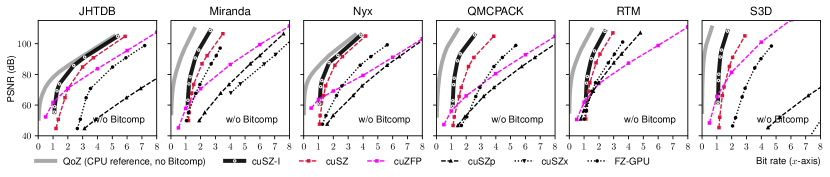
(a) Bit rate-PSNR plots, without Bitcomp.

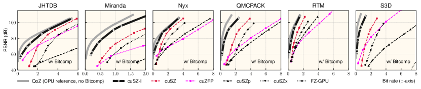
(b) Bit rate-PSNR plots, with Bitcomp.

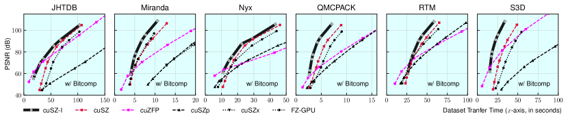
(c) Transfer Time-PSNR plots, with Bitcomp.

Figure 7: Bit rate- and Transfer Time-PSNR curves of compressors on six datasets. A curve positioned toward upper left indicates the advantageous compressor performance in achieving both better fidelity and compression ratios (Fig.  7(a) and 7(b)), or the shorter transfer time (Fig.  7(c)).

(a) Visualization of the original data and the data reconstructed from cuSZ-I (ours), cuZFP, cuSZx, cuSZ, cuSZp, and FZ-GPU on JHTDB.

(b) Selective visualization of the original data and the data reconstructed from cuSZ-I (ours), cuZFP, and cuSZ on datasets Miranda, Nyx, QMCPACK, RTM, and S3D.

Figure 8: Showcase of decompressed data visualizations, with key subregions zoomed in. For each dataset, we align the compression ratio for every compressor to a fixed value. cuSZ, cuSZp, and FZ-GPU share the same Lorenzo predictor, generating similar data visualizations. Hence, we selectively present the visualization of only the original data and the data reconstructed from cuSZ-I, cuZFP, and cuSZ.

VII-B3 Case study: decompression visualizations

To further verify the high compression fidelity of cuSZ-I, we select one data field from each dataset and then visualize the decompressed snapshots. Fig. 8 shows the original and decompression visualization of six data snapshots, together with the compression ratios, error bounds, and PSNRs. For each set of visualizations on the same snapshot, we align the compression ratios to the same value (e.g., $\sim$ 27 for JHTDB). Due to space limit, we propose all 6 decompression visualizations for the JHTDB dataset but show only 3 of them for other datasets.

In all cases, cuSZ-I has the best decompression data visualization quality, closest to the original data with minimized data artifacts. In contrast, all other compressors have presented decompressed data exhibiting severe data visualization artifacts. For the RTM dataset snapshot #2800, under a fixed compression ratio of 80 (or lower for cuSZx since its error bound has been too large), cuSZ-I achieves the decompression PSNR of 80.22, which is 34 higher than the second-highest PSNR from cuSZ (an exceptionally significant gap). On the QMCPACK dataset, cuSZ-I also obtains a decompression PSNR of 88.8, 35 higher than the second-best cuZFP under CR=80.

VII-B4 Compression Throughtputs

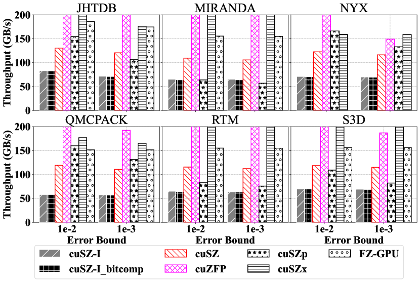
(a) Compression throughputs on NVIDIA A100.

(b) Deompression throughputs on NVIDIA A100.

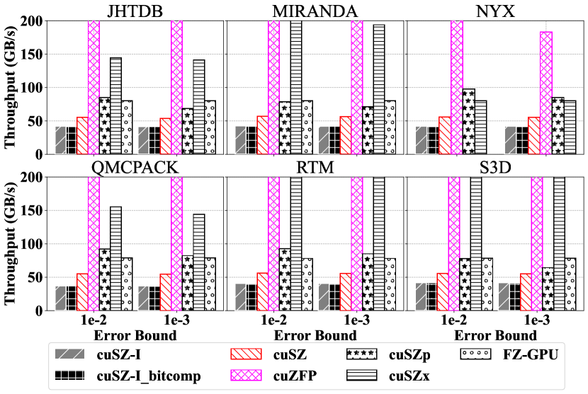
(c) Compression throughputs on NVIDIA A40.

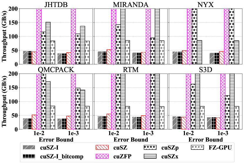
(d) Deompression throughputs on NVIDIA A40.

Figure 9: Compression and decompression throughputs on NVIDIA A100 (top row) and A40 (bottom row) for cuSZ-I, cuSZ-I with Bitcomp, cuSZ, cuZFP, cuSZp, cuSZx, and FZ-GPU. cuZFP’s throughput corresponds to a similar average PSNR with cuSZ-I.

Having seen the high compression ratios and qualities of cuSZ-I, we would like to address the concern of the computational cost and overhead of cuSZ-I. The speed of cuSZ-I is inevitably slower than cuSZ, due to the intrinsic of the interpolation-based predictor, which has more computational operations and less parallelizability than the Lorenzo predictor. Therefore, compared to other compressors, we need to confirm whether the additional computational cost of cuSZ-I is affordable to obtain improvements in compression ratio and quality. Shortly speaking, We have made our best effort to propose an efficient implementation of G-Interp, and it still has some improvement spaces. Therefore, the current compression throughputs of cuSZ-I are arguably acceptable and can be further optimized over time.

We have profiled the compression throughputs of the GPU-based lossy compressors on two platforms (Theta-GPU with NVIDIA TESLA A100 GPU and JLSE with NVIDIA TESLA A40 GPU) using the kernel execution time measured by the NVIDIA Nsight System. Fig. 9(a) and 9(b) demonstrate the compression and decompression throughputs of all the 6 GPU-based compressors under two different error bounds (1e–2 and 1e–3) on the Theta-GPU NVIDIA TESLA A100 platform. In the tables, the term cuSZ-I corresponds to a cuSZ-I pipeline without Bitcomp, and cuSZ-I_bitcomp is the full pipeline cuSZ-I including Bitcomp. We can observe that adding Bitcomp only brings trivial overhead to compression throughputs, and cuSZ-I’s throughput is on the same magnitude as cuSZ and cuSZp, having a compression speed of $\sim$ 60% of cuSZ and a decompression speed of 80% $\sim$ 90% of cuSZ. Fig. 9(c) and 9(d) present throughput profiling results on the JLSE platform with NVIDIA TESLA A40. On this platform, cuSZ-I has a closer performance to cuSZ (its compression throughput is 70% $\sim$ 80% to cuSZ, and the decompression throughput is nearly the same as cuSZ). On those platforms, although cuSZx, cuZFP, and FZ-GPU have relatively higher throughput than cuSZ-I, their compression ratios are much lower than cuSZ-I, making them inadequate for many real-use tasks in which high-ratio compression is needed for minimizing the data storage and transfer costs. Next, we will see how cuSZ-I can show its advantage in that kind of task.

VII-B5 Case study: distributed lossy data transmission

In this part, we present and discuss a practical use case: distributed lossy data transmission. Initially, a distributed scientific database is deployed across several supercomputers. To achieve rapid data transfer and access between two distributed machines within this database system, instead of transferring the original exascale data, which would take an impractical amount of time, the database system transfers only the significantly smaller compressed data. To this end, an error-bounded lossy compressor needs to operate on both the source and destination machines. The overall time required for this process is the sum of local data I/O time, the data compression and decompression time, and the time for transferring the compressed data between the machines. Since the data transfer between remote machines will be performed under relatively low bandwidths, a data compressor with both high ratios and high performance (therefore, GPU-accelerated-ones are preferred) is required to obtain an optimized data transfer efficiency. In Fig. 7(c), we show the plots of data transfer time cost and decompression data PSNR for this task. Specifically, the source machine is ALCF Theta-GPU, and the destination machine is Purdue RCAC Anvil. Since the local I/O time is unstable and irrelevant to the compressors, we compute the overall time with only the data compression/decompression time and the distributed compressed data transfer time. For better and more stable time measurement, each dataset is duplicated by 100 times. The data transfer between 2 machines is managed by Globus [39], having a bandwidth of approximately 1GB/s. Moreover, Bitcomp is applied to all cases to further reduce data transfer costs. As Fig. 7(c) indicates, cuSZ-I has the optimized time cost on all high-quality data transfer cases (PSNR $\leq$ 70). On specific data transfer tasks with low-quality data, cuSZ-I is also very competitive. For the QMCPACK dataset, cuSZ-I can reduce around 30% of the time cost of the second-best cuSZ for transferring the dataset with PSNR=90. For the S3D dataset, it can reduce around 40% of the time cost of the second-best cuZFP for transferring the dataset with PSNR=80. Concluded from those results, we can convincingly state that the high compression ratio and quality of cuSZ-I have well compensated for its speed degradation, exhibiting great potential to be applied to a large variety of real-world use cases in which compression ratio and compression throughput are both highly concerned.

VII-B6 Ablation study: disassemble the auto-tuning module of cuSZ-I

In §V-E, we detail the advantages of the interpolation-based predictor over the Lorenzo predictor. To examine the effectiveness of G-Interp auto-tuning module in cuSZ-I, we conduct an ablation study analyzing each single design component of it. In Fig. 10 (a), we present the compression rate-distortion of cuSZ, cuSZ-I (without an autotuning model), and cuSZ-I (with the dimension sequence auto-tuning) on the transposed V field of the SCALE-LetKF [40]. Since the fastest-varying dimension of this data is very unsmooth, cuSZ-i applying the default interpolation dimension sequence shows very limited compression ratios lower than the cuSZ. However, after reordering the interpolation dimensions by auto-tuning, the compression quality of cuSZ-I has largely improved. In Fig. 10 (b), we compare the compression rate-distortion of cuSZ-I under different configurations (no auto-tuning, only adjust the level-wise error bounds and the full auto-tuning including the cubic spline selection). From the plot, We can find that both the level-wise error-bound tuning and the cubic spline selection benefit the overall rate-distortion of cuSZ-I compression.

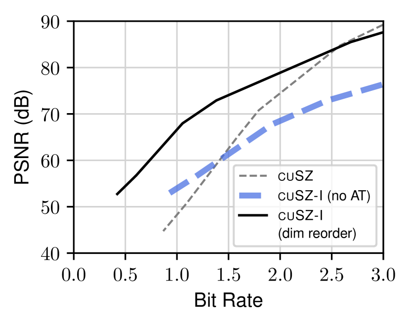
(a) SCALE-LetKF-V (transposed).

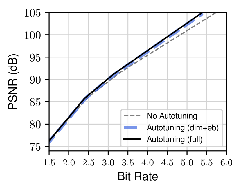
(b) JHTDB

Figure 10: Ablation Studies of auto-tuning components.

VIII Conclusion and Future Work

In this work, we propose cuSZ-I, an efficient GPU-accelerated scientific error-bounded lossy compressor, which exhibits the best compression quality compared with other related works based on our experiments. With a software-hardware codesign of highly parallelized interpolation-based data predictor and a lightweight auto-tuning kernel, cuSZ-I achieves state-of-the-art compression quality under the same error bounds or compression ratios by its high data prediction accuracy. Combining an improved implementation of Huffman encoding and the NVIDIA Bitcomp lossless module, cuSZ-I also outperforms other GPU-accelerated scientific lossy compressors in terms of compression ratios by significant gaps, approaching CPU-based compressors meanwhile having far higher throughputs than them. In several case studies, cuSZ-I presents excellent decompression data visualization that prevails over existing state-of-the-art GPU-accelerated lossy compressors, and reduces the distributed lossy data transmission time to a considerable extent for distributed scientific databases.

So far, cuSZ-I has a few limitations: e.g., its compression speeds are slower than other GPU compressors, its interpolation-based prediction still having lower accuracy than the CPU-based interpolators, and certain part of its lossless module is based on the NVIDIA GPU architecture. In the future, we will endeavor to address those limitations, working on improving its speeds, prediction accuracy, and compatibility with more GPU architectures such as AMD and Intel GPUs.

References

- [1] Salman Habib et al. “HACC: Extreme scaling and performance across diverse architectures” In Communications of the ACM 60.1 ACM, 2016, pp. 97–104
- [2] S. Crusan V. Vishwanath and K. Harms “Parallel I/O on Mira” Online, https://www.alcf.anl.gov/files/Parallel_IO_on_Mira_0.pdf, 2019
- [3] Dirk Meister et al. “A study on data deduplication in HPC storage systems” In SC ’12: Proceedings of the International Conference on High Performance Computing, Networking, Storage and Analysis Salt Lake City, UT, USA: IEEE, 2012, pp. 7
- [4] Seung Woo Son et al. “Data compression for the exascale computing era-survey” In Supercomputing Frontiers and Innovations 1.2, 2014, pp. 76–88
- [5] Xin Liang et al. “Error-controlled lossy compression optimized for high compression ratios of scientific datasets” In 2018 IEEE International Conference on Big Data (Big Data) Seattle, WA, USA: IEEE, 2018, pp. 438–447
- [6] Xin Liang et al. “SZ3: A modular framework for composing prediction-based error-bounded lossy compressors” In IEEE Transactions on Big Data IEEE, 2022
- [7] Jinyang Liu et al. “Dynamic quality metric oriented error bounded lossy compression for scientific datasets” In 2022 SC22: International Conference for High Performance Computing, Networking, Storage and Analysis (SC), 2022, pp. 892–906 IEEE Computer Society
- [8] Shaomeng Li, Peter Lindstrom and John Clyne “Lossy scientific data compression with SPERR” In 2023 IEEE International Parallel and Distributed Processing Symposium (IPDPS), 2023, pp. 1007–1017 IEEE
- [9] Online, https://lcls.slac.stanford.edu/lasers/lcls-ii
- [10] Franck Cappello et al. “Use cases of lossy compression for floating-point data in scientific data sets” In The International Journal of High Performance Computing Applications 33.6 SAGE Publications Sage UK: London, England, 2019, pp. 1201–1220
- [11] Jiannan Tian et al. “Cusz: An efficient gpu-based error-bounded lossy compression framework for scientific data” In Proceedings of the ACM International Conference on Parallel Architectures and Compilation Techniques, 2020, pp. 3–15
- [12] J. Tian et al. “Optimizing Error-Bounded Lossy Compression for Scientific Data on GPUs” In 2021 IEEE International Conference on Cluster Computing (CLUSTER) Los Alamitos, CA, USA: IEEE Computer Society, 2021, pp. 283–293 DOI: 10.1109/Cluster48925.2021.00047
- [13] Xiaodong Yu et al. “SZX: An ultra-fast error-bounded lossy compressor for scientific datasets” In arXiv preprint arXiv:2201.13020, 2022
- [14] Boyuan Zhang et al. “FZ-GPU: A Fast and High-Ratio Lossy Compressor for Scientific Computing Applications on GPUs” In arXiv preprint arXiv:2304.12557, 2023
- [15] Yafan Huang et al. “cuSZp: An Ultra-fast GPU Error-bounded Lossy Compression Framework with Optimized End-to-End Performance” In Proceedings of the International Conference for High Performance Computing, Networking, Storage and Analysis, 2023, pp. 1–13
- [16] cuZFP Online, https://github.com/LLNL/zfp/tree/develop/src/cuda_zfp, 2019
- [17] Gregory K Wallace “The JPEG still picture compression standard” In IEEE Transactions on Consumer Electronics 38.1 IEEE, 1992, pp. xviii–xxxiv
- [18] Didier Le Gall “MPEG: A video compression standard for multimedia applications” In Communications of the ACM 34.4 ACM New York, NY, USA, 1991, pp. 46–58
- [19] Kai Zhao et al. “Optimizing Error-Bounded Lossy Compression for Scientific Data by Dynamic Spline Interpolation” In 2021 IEEE 37th International Conference on Data Engineering (ICDE), 2021, pp. 1643–1654 IEEE
- [20] Peter Lindstrom “Fixed-rate compressed floating-point arrays” In IEEE Transactions on Visualization and Computer Graphics 20.12 IEEE, 2014, pp. 2674–2683
- [21] Rafael Ballester-Ripoll, Peter Lindstrom and Renato Pajarola “TTHRESH: Tensor compression for multidimensional visual data” In IEEE transactions on visualization and computer graphics 26.9 IEEE, 2019, pp. 2891–2903
- [22] Jinyang Liu et al. “Exploring Autoencoder-based Error-bounded Compression for Scientific Data” In 2021 IEEE International Conference on Cluster Computing (CLUSTER), 2021, pp. 294–306 IEEE
- [23] Jinyang Liu et al. “Exploring autoencoder-based error-bounded compression for scientific data” In 2021 IEEE International Conference on Cluster Computing (CLUSTER), 2021, pp. 294–306 IEEE
- [24] Jun Han and Chaoli Wang “Coordnet: Data generation and visualization generation for time-varying volumes via a coordinate-based neural network” In IEEE Transactions on Visualization and Computer Graphics IEEE, 2022
- [25] Zstd Online, https://github.com/facebook/zstd/releases, 2019
- [26] Dingwen Tao, Sheng Di, Zizhong Chen and Franck Cappello “Significantly improving lossy compression for scientific data sets based on multidimensional prediction and error-controlled quantization” In 2017 IEEE International Parallel and Distributed Processing Symposium Orlando, FL, USA: IEEE, 2017, pp. 1129–1139
- [27] Jinyang Liu et al. “High-performance Effective Scientific Error-bounded Lossy Compression with Auto-tuned Multi-component Interpolation” In arXiv preprint arXiv:2311.12133, 2023
- [28] Jinyang Liu et al. “FAZ: A flexible auto-tuned modular error-bounded compression framework for scientific data” In Proceedings of the 37th International Conference on Supercomputing, 2023, pp. 1–13
- [29] Miranda Radiation Hydrodynamics Data Online, https://wci.llnl.gov/simulation/computer-codes/miranda, 2019
- [30] Jiannan Tian et al. “Revisiting Huffman Coding: Toward Extreme Performance on Modern GPU Architectures” In 2021 IEEE International Parallel and Distributed Processing Symposium (IPDPS), Portland, OR, USA, May 17-21, 2021 IEEE, 2021, pp. 881–891
- [31] Boyuan Zhang et al. “GPULZ: Optimizing LZSS Lossless Compression for Multi-byte Data on Modern GPUs” In Proceedings of the 37th International Conference on Supercomputing, 2023, pp. 348–359
- [32] NVIDIA Online, https://developer.nvidia.com/nvcomp
- [33] “Theta/ThetaGPU - Argonne Leadership Computing Facility” (Accessed on 05/21/2021), https://www.alcf.anl.gov/support-center/theta/theta-thetagpu-overview
- [34] Scientific Data Reduction Benchmarks Online, https://sdrbench.github.io/, 2019
- [35] Yi Li et al. “A public turbulence database cluster and applications to study Lagrangian evolution of velocity increments in turbulence” In Journal of Turbulence Taylor & Francis, 2008, pp. N31
- [36] NYX simulation Online, https://amrex-astro.github.io/Nyx/
- [37] QMCPACK: many-body ab initio Quantum Monte Carlo code Online, http://vis.computer.org/vis2004contest/data.html, 2019
- [38] Suha Kayum “GeoDRIVE – a high performance computing flexible platform for seismic applications” In First Break 38.2, 2020, pp. 97–100
- [39] Rachana Ananthakrishnan, Kyle Chard, Ian Foster and Steven Tuecke “Globus platform-as-a-service for collaborative science applications” In Concurrency and Computation: Practice and Experience 27.2 Wiley Online Library, 2015, pp. 290–305
- [40] “Scalable Computing for Advanced Library and Environment (SCALE) – LETKF”, https://github.com/gylien/scale-letkf