Phase diagrams of quasinormal frequencies for Schwarzschild, Kerr, and Taub-NUT black holes

Abstract

The Newman-Janis algorithm, which involves complex-coordinate transformations, establishes connections between static and spherically symmetric black holes and rotating and/or axially symmetric ones, such as between Schwarzschild black holes and Kerr black holes, and between Schwarzschild black holes and Taub-NUT black holes. However, the transformations in the two samples are based on different physical mechanisms. The former connection arises from the exponentiation of spin operators, while the latter from a duality operation. In this paper, we mainly investigate how the connections manifest in the dynamics of black holes. Specifically, we focus on studying the correlations of quasinormal frequencies among Schwarzschild, Kerr, and Taub-NUT black holes. This analysis allows us to explore the physics of complex-coordinate transformations in the spectrum of quasinormal frequencies.

1 Introduction

Gravitational waves (GWs) were first predicted by Albert Einstein in his general theory of relativity in 1916. However, they were not observed until 2015 by the Laser Interferometer Gravitational-Wave Observatory (LIGO) [1, 2]. Since then, the detection of GWs has opened up [3, 4] a new era of multimessenger astronomy, where GW signals are combined with electromagnetic observations.

The observation from the LIGO was the result of the merging of two black holes (BHs) in a binary system. Binary BHs are pairs of BHs [5] that orbit around each other. As they move closer together, they release energy in the form of GWs. This energy loss causes the BHs to spiral inward, eventually resulting in a cataclysmic merger. When the BHs merge, they create intense GWs that propagate outward through the universe. These waves carry crucial information about the astrophysical processes involved in the merger, as well as the properties of the BHs themselves.

Quasinormal modes (QNMs) or quasinormal frequencies (QNFs) are a fundamental concept [6] in the study of GWs. This physical quantity describes a set of damping modes, where its real part determines the oscillation of GWs, while its imaginary part the damping rate that describes how quickly the oscillations decay over time. When two BHs merge, the emitted GWs change gradually from oscillation to exponential decay. These modes provide important information about the properties of the BHs. The analysis of QNFs in GW signals opens up new avenues for exploring the mysteries of the universe and the fundamental nature of gravity.

The Newman-Janis algorithm (NJA) is a mathematical method [7] that exploits complex-coordinate transformations to convert a static and spherically symmetric BH solution to a rotating and/or axially symmetric one. In the study of regular black holes (RBHs) [8, 9, 10, 11, 12], this algorithm is notable for two reasons. At first, it can generate rotating RBHs from a static seed, see the current review articles [13, 14] and the references therein. Secondly, it has the capability to modify or remove the curvature singularities of singular black holes (SBHs).

As an example, the NJA can transform [7] Schwarzschild BHs into Kerr BHs through the following transformations,

$$u\to u-\mathrm{i}a\cos\theta,\qquad r\to r+\mathrm{i}a\cos\theta,$$ (1a)

together with such complexifications,

$$\frac{1}{r}\to\frac{\real[r]}{\absolutevalue{r}^{2}},\qquad r^{2}\to\absolutevalue{r}^{2}.$$ (1b)

Here, $a$ denotes rotation parameter and $u$ “time” in the Eddington-Finkelstein coordinate. The underlying physical mechanism of the connection between Schwarzschild and Kerr BHs was established [15] through the exponentiation of spin operators, where a three-point amplitude was considered in the minimal coupling of spinning particles and gravitons.

Now let us turn to the change in singularity. The Kretschmann scalar of Schwarzschild BHs, which is a measure of curvatures, is proportional to $r^{-6}$ around $r=0$. After the complexification, $r^{2}$ becomes $\absolutevalue{r}^{2}$ and the radial coordinate takes a shift, $r\to r+\mathrm{i}a\cos\theta$, and then the singular point $r=0$ changes into a singular ring described by $r^{2}+a^{2}\cos^{2}\theta=0$. In other words, the NJA alters the type of singular curvatures, from point singularity to ring singularity, when it is applied to Schwarzschild BHs.

As another example, by using the alternative transformations [16],

$$u\to u-2\mathrm{i}N\ln\sin\theta,\qquad r\to r-\mathrm{i}N,\qquad M\to M-\mathrm{i}N,$$ (2a)

together with the corresponding complexifications,

$$\frac{1}{r}\to\frac{\real[Mr]}{\absolutevalue{r}^{2}},\qquad r^{2}\to\absolutevalue{r}^{2},$$ (2b)

one can convert Schwarzschild BHs into Taub-NUT BHs, where $N$ denotes a NUT charge. The relationship between Schwarzschild BHs and Taub-NUT BHs can be understood [17] as a duality operation. In other words, it can be seen as a gravitational analog of electric-magnetic duality. Moreover, the “singularities” are determined by the zeros of the algebraic equation, $r^{2}+N^{2}=0$, indicating that there is no curvature singularity along the real axis of $r$. This implies that the curvature singularity of Schwarzschild BHs has been removed. This phenomenon can also be seen in the Stokes portrait [18], where the singularity is actually pushed onto the imaginary axis (non-physical domain).

As demonstrated above, one can deduce rotating or axially aymmetric BHs, Kerr or Taub-NUT, from the same static and spherically symmetric seed, Schwarzschild BHs, by using different transformations of the NJA. We are interested in dynamical differences hidden behind the different mathematical transformations because Kerr and Taub-NUT BHs are obviously distinct in some crucial properties, such as the singularity as mentioned above. In other words, we want to reveal the physics that is hidden behind mathematics (NJA transformations). Specifically, we mainly investigate how the different connections, between Schwarzschild and Kerr BHs and between Schwarzschild and Taub-NUT BHs, manifest in the QNFs, one of the significant features in dynamics of BHs.

The paper is arranged as follows. In Sec. 2, we analyze how the singularities of Kerr-Taub-NUT BHs change in the parameter space of $(a,N)$. We then present in Sec. 3 the analytical QNFs of Schwarzschild, Kerr, and Taub-NUT BHs through the light ring/QNMs correspondence. In order to acquire more accurate QNFs than the analytical ones from the light ring/QNMs correspondence, we need to perform numerical calculations as proceeded in the following three sections. In Sec. 4, we discuss two types of test-field perturbations: scalar fields and spinor fields, with and without mass, where we focus on the separation of variables. Further, we explore the spectrum of angular equations in Sec. 5. We investigate the connections in the spectra of QNFs for Schwarzschild, Kerr, and Taub-NUT BHs in Sec. 6. Finally, we present our conclusions in Sec. 7. App. A gives the coefficients of recursion formulas when we calculate the spectra of QNFs numerically by using Leaver’s method.

2 Kerr-Taub-NUT black holes and curvature invariants

To facilitate subsequent discussions, we combine the Kerr and Taub-NUT BHs into a single entity, referred to in literature as the Kerr-Taub-NUT spacetime [19]. In the Boyer-Lindquist coordinates $(t,r,\theta,\phi)$, the metric of Kerr-Taub-NUT BHs can be expressed [20] in the following form,

$$\mathrm{d}s^{2} = -\frac{\Delta}{\Sigma}\left[\mathrm{d}t+(2N\cos{\theta}-a\sin^{2}{\theta})\mathrm{d}\phi\right]^{2}+\frac{\Sigma}{\Delta}\mathrm{d}r^{2}$$ (3)

$$+\frac{\sin^{2}{\theta}}{\Sigma}\left[-a\mathrm{d}t+(r^{2}+a^{2}+N^{2})\mathrm{d}\phi\right]^{2}+\Sigma\mathrm{d}\theta^{2},$$

where $\Sigma$ and $\Delta$ are defined by

$$\begin{split}\Sigma=\Sigma_{1}\Sigma_{2},\qquad\Sigma_{1}=r+\mathrm{i}(a\cos{\theta}+N),\qquad\Sigma_{2}=r-\mathrm{i}(a\cos{\theta}+N),\end{split}$$ (4a)

$$\begin{split}\Delta=r^{2}-2Mr+a^{2}-N^{2}.\end{split}$$ (4b)

Eq. (3) describes Schwarzschild, Kerr, and Taub-NUT BHs, respectively, depending on the different regions of the parameter space $(a,N)$.

• If both $a$ and $N$ vanish, Eq. (3) reduces to the metric of Schwarzschild BHs;

• If $a$ does not vanish but $N$ does, Eq. (3) reduces to the metric of Kerr BHs;

• If $a$ vanishes but $N$ does not, Eq. (3) reduces to the metric of Taub-NUT BHs.

Next, we turn to the curvature invariants of Kerr-Taub-NUT BHs, where they are composed of a complete set and referred to as Zakhary-Mcintosh invariants [21]. This set contains seventeen elements and can be classified [14] into three groups: the Ricci type, solely constructed from Ricci tensors; the Weyl type, solely constructed from Weyl tensors; and the mixed type, constructed from both Ricci and Weyl tensors.

Because the Ricci tensor of Eq. (3) equals zero, $R_{\mu\nu}=0$, the curvature invariants derived by the contraction of Ricci tensors also equal zero. As a result, both the Ricci and mixed types are vanishing, and our calculations depend [14] only on the four elements in the Weyl type. The denominators of these four invariants are all proportional to the factor, $(N+a\cos\theta)^{2}+r^{2}$, which gives the singularities as follows:

$$r=0,\qquad N+a\cos\theta=0,$$ (5)

or in the Cartesian coordinates $(t,x,y,z)$ as follows [22]:

$$x^{2}+y^{2}=a^{2}-N^{2},\qquad z=0.$$ (6)

Thus, we divide the singularities into three classes according to the parameter space $(a,N)$:

• If $a^{2}>N^{2}$, singular rings appear in the $x-y$ plane;

• If $a^{2}=N^{2}$, a singular point appears at the center;

• If $a^{2}<N^{2}$, no singularities appear.

We note that the singularities mentioned above are unrelated to the mass parameter. Furthermore, Kerr-Taub-NUT BHs manifest in two distinct phases in terms of the parameter space $(a,N)$ if the rotation parameter $a$ decreases from $a^{2}>N^{2}$ to $a^{2}<N^{2}$ for a fixed $N$ and simultaneously if the Kerr-Taub-NUT spacetime still exists. In one phase Kerr-Taub-NUT BHs contain singular rings in the case of $a^{2}>N^{2}$, while in the other phase Kerr-Taub-NUT BHs do not have curvature singularities in the case of $a^{2}<N^{2}$, where the two phases are separated by the configuration of Kerr-Taub-NUT BHs that possesses one singular point in the case of $a^{2}=N^{2}$.

3 Analytical QNMs by the light ring/QNMs correspondence

We provide the analytical QNMs of Schwarzschild, Kerr, and Taub-NUT BHs using the light ring/QNMs correspondence [23], which connects the QNFs to circular null geodesics, known as photon spheres, in the eikonal limit,

$$\omega=\Omega_{c}l-\mathrm{i}\left(n+\frac{1}{2}\right)\lambda_{c},$$ (7)

where $\Omega_{c}$ denotes the angular velocity when a particle stays at an unstable null geodesic, $\lambda_{c}$ the Lyapunov exponent, $l$ the multipole number, and $n$ the overtone number.

In order to determine the circular null geodesics of test particles $\phi$ in the Kerr-Taub-NUT spacetime, one calculates [24, 25] the effective potential of the radial equation of particles,

$$V_{r}=E^{2}+\frac{2Mr+2N^{2}}{(r^{2}+N^{2})^{2}}(aE-L)^{2}+\frac{a^{2}E^{2}-L^{2}}{r^{2}+N^{2}},$$ (8a)

the time-component equation with respect to the proper time,

$$\dot{t}=\frac{1}{\Delta}\left[\left(r^{2}+N^{2}+a^{2}+a^{2}\frac{2Mr+2N^{2}}{r^{2}+N^{2}}\right)E-\frac{a(2Mr+2N^{2})}{r^{2}+N^{2}}L\right],$$ (8b)

and the $$\phi$$ equation with respect to the proper time,

$$\dot{\phi}=\frac{1}{\Delta}\left[\frac{r^{2}-2Mr-N^{2}}{r^{2}+N^{2}}L+\frac{2a(Mr+N^{2})}{r^{2}+N^{2}}E\right].$$ (8c)

Further, one gives the radius of photon spheres by $V_{r}=V^{\prime}_{r}=0$,

$$r_{c}^{3}-3Mr_{c}^{2}-3N^{2}r_{c}\pm 2a\sqrt{r_{c}(Mr_{c}^{2}+2N^{2}r_{c}-MN^{2})}+MN^{2}=0.$$ (9)

Thus, the angular frequency and Lyapunov exponent on the surface of photon spheres take the forms,

$$\Omega_{c}=\frac{\dot{\phi}}{\dot{t}}\Big{|}_{r=r_{c}},\qquad\lambda_{c}=\sqrt{\frac{V^{\prime\prime}_{r}}{2\dot{t}^{2}}}\Big{|}_{r=r_{c}},$$ (10)

from which one obtains that the angular frequency is exactly equal to the inverse of impact parameter $D_{c}$,

$$\Omega_{c}=\frac{1}{D_{c}},\qquad D_{c}^{2}=a^{2}+(r_{c}^{2}+N^{2})\frac{3Mr_{c}^{2}+4N^{2}-MN^{2}}{Mr_{c}^{2}+2N^{2}r_{c}-MN^{2}}.$$ (11)

Next, we shall compute the QNFs for the three BHs and compare their results.

3.1 Schwarzschild black holes

For Schwarzschild BHs, $a=N=0$, the equation of photon spheres has only one root outside the horizon, i.e., we derive the radius of horizons and the radius of photon spheres,

$$r^{\rm Sch}_{\rm H}=2M,\qquad r^{\rm Sch}_{c}=3M,$$ (12)

respectively, and then the impact parameter using Eq. (11),

$$D^{\rm Sch}_{c}=3\sqrt{3}M.$$ (13)

As a result, we conclude that the angular frequency equals the Lyapunov exponent by considering Eqs. (8), (12), and (10),

$$\Omega_{c}^{\rm Sch}=\lambda^{\rm Sch}_{c}=\frac{1}{3\sqrt{3}M},$$ (14)

which contains all the information of QNFs in the eikonal limit based on the light ring/QNMs correspondence Eq. (7).

3.2 Kerr black holes

For Kerr BHs, the horizon exists if $M>\absolutevalue{a}$, i.e.,

$$r^{\rm Ker}_{\rm H}=M+\sqrt{M^{2}-a^{2}},$$ (15)

and the radius of photon spheres for corotating geodesics takes the following form in terms of Eq. (9) together with $N=0$,

$$r^{\rm Ker}_{c}=M+y\sqrt{M^{2}-a^{2}},$$ (16)

where $y$ is a dimensionless parameter defined by

$$y=\frac{1}{\sqrt{1-\frac{a^{2}}{M^{2}}}}+\frac{2}{\sqrt{1-\frac{a^{2}}{M^{2}}}}\cos\left(\frac{1}{3}\arg\left[2\frac{a}{M}\left(\sqrt{\frac{a^{2}}{M^{2}}-1}+\frac{a}{M}\right)-1\right]\right).$$ (17)

We note that $y$ is a monotonic increasing function of $a/M$ and it has the following limit,

$$\lim_{a/M\to 0}y=2,$$ (18)

which shows that the photon sphere is outside the horizon. Substituting $N=0$ into Eq. (11), we obtain the angular frequency and the impact parameter,

$$\Omega_{c}^{\rm Ker}=\frac{1}{D_{c}^{\rm Ker}}=\frac{1}{\sqrt{3r_{c}^{2}+a^{2}}},$$ (19)

and using Eqs. (8), (16), and (10), we can derive the Lyapunov exponent from the following ratio,

$$\frac{\lambda_{c}^{\rm Ker}}{\Omega_{c}^{\rm Ker}}=\frac{\left[a^{2}+r_{c}(r_{c}-2M)\right]\sqrt{3r_{c}(a-D_{c})[4M(a-D_{c})+r_{c}(a+D_{c})]}}{r_{c}^{2}[2aM+D_{c}(r_{c}-2M)]}.$$ (20)

3.3 Taub-NUT black holes

The horizon of Taub-NUT BHs is not less than that of Schwarzschild BHs,

$$r_{\rm H}^{\rm NUT}=M+\sqrt{M^{2}+N^{2}}.$$ (21)

The radius of photon spheres can be cast in the form similar to that of Kerr BHs, but with a different parameter $z$ owing to the substitution of $a=0$ into Eq. (9),

$$r_{c}^{\rm NUT}=M+z\sqrt{M^{2}+N^{2}},\qquad z=2\cos\left(\frac{1}{3}\tan^{-1}\frac{N}{M}\right),$$ (22)

where $z$ is a monotonic decreasing function of $N/M$ and has the following limits,

$$\lim_{N/M\to 0}z=2,\qquad\lim_{N/M\to\infty}z=\sqrt{3}>1,$$ (23)

which, like the case of Kerr BHs, shows that the photon sphere is outside the horizon. Substituting $a=0$ into Eq. (11), we obtain the angular frequency and the impact parameter,

$$\Omega_{c}^{\rm NUT}=\frac{1}{D_{c}^{\rm NUT}}=\sqrt{\frac{M\left(r_{c}^{2}-N^{2}\right)+2N^{2}r_{c}}{\left(N^{2}+r_{c}^{2}\right)\left(-MN^{2}+3Mr_{c}^{2}+4N^{2}r_{c}\right)}},$$ (24)

and using Eqs. (8), (22), and (10), we can derive the Lyapunov exponent from the following ratio,

$$\frac{\lambda_{c}^{\rm NUT}}{\Omega_{c}^{\rm NUT}}=\frac{\sqrt{3\left[2N^{2}r_{c}(3r_{c}-2M)+r_{c}^{3}(4M-r_{c})-N^{4}\right]}}{N^{2}+r_{c}^{2}}.$$ (25)

3.4 Analysis of quasinormal frequencies

We give two comments about QNFs depicted by Eq. (7). The first is that Eq. (7) is applicable only under the eikonal limit, where the multipole number (angular momentum) $l$ is much larger than one and then its contribution is much larger than that of spins. Consequently, the QNFs do not encompass any spin characteristics. The second comment is that the real part of QNFs is affected by the multipole number $l$ but not by the overtone number $n$, and the imaginary part is affected by the overtone number $n$ but not by the multipole number $l$. This implies that the real part displays a positive correlation with the multipole number $l$, and the imaginary part does with the overtone number $n$.

Now let us analyze the asymptotic behaviors of $\Omega_{c}$ and $\lambda_{c}$. When the rotation parameter $a\to 0$ for Kerr BHs and the NUT charge $N\to 0$ for Taub-NUT BHs, the leading terms of $\Omega_{c}$ and $\lambda_{c}$ for the two BHs must be consistent with those of Schwarzschild BHs,

$$\Omega_{c}^{\rm Ker}\sim\frac{1}{3\sqrt{3}M}+\frac{2a}{27M^{2}}+O\left(a^{2}\right),$$ (26a)

$$\lambda_{c}^{\rm Ker}\sim\frac{1}{3\sqrt{3}M}-\frac{2a^{2}}{81\sqrt{3}M^{3}}+O\left(a^{3}\right),$$ (26b)

and

$$\Omega_{c}^{\rm NUT}\sim\frac{1}{3\sqrt{3}M}-\frac{5N^{2}}{54\sqrt{3}M^{3}}+O\left(N^{3}\right),$$ (27a)

$$\lambda_{c}^{\rm NUT}\sim\frac{1}{3\sqrt{3}M}-\frac{11N^{2}}{162\sqrt{3}M^{3}}+O\left(N^{3}\right).$$ (27b)

This is not difficult for us to understand from physics since both Kerr and Taub-NUT BHs reduce to Schwarzschild BHs when $a\to 0$ and $N\to 0$, respectively.

In accordance with Eqs. (14), (26), and (27), we compare angular velocities and Lyapunov exponents between Kerr and Schwarzschild BHs, between Taub-NUT and Schwarzschild BHs, and between Taub-NUT and Kerr BHs, respectively,

$$\Omega_{c}^{\rm Ker}/\Omega_{c}^{\rm Sch}>1,\qquad\lambda_{c}^{\rm Ker}/\lambda_{c}^{\rm Sch}<1,$$ (28)

$$\Omega_{c}^{\rm NUT}/\Omega_{c}^{\rm Sch}<1,\qquad\lambda_{c}^{\rm NUT}/\lambda_{c}^{\rm Sch}<1,$$ (29)

$$\Omega_{c}^{\rm NUT}/\Omega_{c}^{\rm Ker}<1,\qquad\lambda_{c}^{\rm NUT}/\lambda_{c}^{\rm Ker}<1.$$ (30)

Based on the above inequalities, we observe that the rotation parameter $a$ is associated with an increase in the oscillation frequency ($\Omega_{c}^{\rm Ker}/\Omega_{c}^{\rm Sch}>1$), whereas the NUT charge $N$ is linked to a decrease in the oscillation frequency ($\Omega_{c}^{\rm NUT}/\Omega_{c}^{\rm Sch}<1$ and $\Omega_{c}^{\rm NUT}/\Omega_{c}^{\rm Ker}<1$). Moreover, we notice that both the rotation parameter $a$ and the NUT charge $N$ result in a weakening decay ($\lambda_{c}^{\rm Ker}/\lambda_{c}^{\rm Sch}<1$, $\lambda_{c}^{\rm NUT}/\lambda_{c}^{\rm Sch}<1$, and $\lambda_{c}^{\rm NUT}/\lambda_{c}^{\rm Ker}<1$). Therefore, we may refer Kerr BHs as a counterpart of Schwarzschild BHs with an increasing frequency owing to $\Omega_{c}^{\rm Ker}-\Omega_{c}^{\rm Sch}>0$, while Taub-NUT BHs as a counterpart of Schwarzschild BHs with a decreasing frequency owing to $\Omega_{c}^{\rm NUT}-\Omega_{c}^{\rm Sch}<0$.

Opposite to the limit of $a\to 0$ for Kerr BHs, we now consider the limit of $a\to M$, under which $\Omega_{c}^{\rm Ker}$ goes to a constant $1/(2M)$, and $\lambda_{c}^{\rm Ker}$ vanishing,

$$\Omega_{c}^{\rm Ker}\sim\frac{1}{2M}+\frac{\sqrt{3\left(M-a\right)}}{2\sqrt{2}M^{3/2}}+O\left((a-M)^{1}\right),$$ (31a)

$$\lambda_{c}^{\rm Ker}\sim-\frac{\sqrt{M-a}}{\sqrt{2}M^{3/2}}+O\left((a-M)^{1}\right).$$ (31b)

In other words, when $a$ approaches $M$, Kerr BHs reach a stable state without any decay. For Taub-NUT BHs, both $\Omega_{c}^{\rm NUT}$ and $\lambda_{c}^{\rm NUT}$ vanish when the NUT charge goes to infinity instead of zero,

$$\Omega_{c}^{\rm NUT}\sim\frac{1}{2\sqrt{2}N}+O\left(N^{-2}\right),$$ (32a)

$$\lambda_{c}^{\rm NUT}\sim\frac{\sqrt{3}}{4N}+O\left(N^{-2}\right).$$ (32b)

Combining the above properties of the QNFs for Schwarzschild, Kerr, and Taub-NUT BHs, we depict the QNFs in Fig. 1, where the QNFs of Reissner-Nordström (RN) BHs are attached as a comparison. This diagram illustrates how the QNFs vary with the parameters, such as the mass $M$ for Schwarzschild BHs, the rotation parameter $a$ and mass $M$ for Kerr BHs, and the NUT charge $N$ and mass $M$ for Taub-NUT BHs, and with the parameter — electric charge $Q$ and mass $M$ for RN BHs.

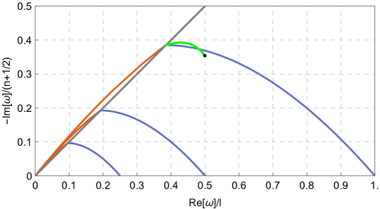
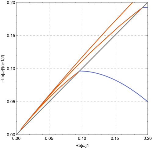
Figure 1: Phase diagram of QNFs (up graph), where the abscissa axis denotes Re($\omega)/l$, i.e., the angular velocity $\Omega_{c}$, and the vertical axis stands for $-{\rm Im}(\omega)/(n+1/2)$, i.e., the Lyapunov exponent $\lambda_{c}$. The gray line represents the case of Schwarzschild BHs, where the QNFs change with respect to the mass $M$. The three blue curves give the QNFs of Kerr BHs that change with respect to the rotation parameter $a$, where $M$ takes $1/2$, $1$, and $2$ from top to bottom, respectively. The three orange curves denote the QNFs of Taub-NUT BHs that change with respect to the NUT charge $N$, where $M$ also takes $1/2$, $1$, and $2$ from top to bottom, respectively. The green curve shows the case of RN BHs, i.e., the QNFs vary with the charge for a fixed $M=1/2$, where the black dot means that the charge takes its maximal value, i.e., the mass of RN BHs. The below graph is amplification of part of the up one for Re($\omega)/l$ being $0$ to $0.2$.

The QNFs of Schwarzschild BHs, see Eq. (14), which change only with the mass $M$, divide the entire QNF plane into two distinct regions, where the QNFs of Kerr BHs are located in the right region while those of Taub-NUT BHs in the left one. We may refer the two regions as two phases, i.e., the Kerr phase and Taub-NUT phase. In other words, we think that Kerr and Taub-NUT BHs are two different states of Schwarzschild BHs in the complex plane of QNFs, and regard Fig. 1 as a dynamical phase diagram in which the QNFs of Schwarzschild BHs represent a coexistence line. The QNFs of Kerr BHs are located in the right side of the coexistence line, while the QNFs of Taub-NUT BHs in the left side. Additionally, when the rotation parameter $a$ goes to the mass for Kerr BHs and the NUT charge $N$ goes to infinity for Taub-NUT BHs, their Lyapunov exponents are vanishing, which implies that the corresponding QNMs become long-lived modes. We may conclude that the above correlations of QNFs (QNMs) are closely connected to the NJA among Schwarzschild, Kerr, and Taub-NUT BHs. In other words, we may speculate that the connections to the NJA give rise to the correlation of QNFs, which may be referred to as the Schwarzschild/Kerr/Taub-NUT (SKT) correspondence, as shown in Fig. 1.

The green curve depicts the variation of QNFs with respect to electric charge $Q$ for RN BHs. The black dot represents the termination of QNFs, which occurs when the charge Q equals the mass $M$. This is easy to be understood because no event horizons exist if the charge is larger than the mass. It is evident that the geometric characteristic of the QNFs of RN BHs is distinct from that of the other three BHs because RN BHs have no connections to any of the three BHs by the NJA.

We end this section by discussing the possibility of a phase transition that occurs in the SKT phases. When we plot the QNFs of Schwarzschild, Kerr, and Taub-NUT BHs in one diagram, it is natural to ask whether a transition between any two of the three phases occurs or not. The answer is negative, owing to the singularity or topological nature of the three BHs. In Sec. 2, we have categorized the singularities of Kerr-Taub-NUT BHs in terms of the parameter space $(a,N)$. The curvature singularities of Schwarzschild, Kerr, and Taub-NUT BHs differ significantly, and the change of curvature singularities from one type to another implies [26] a change in topology. In other words, the difference in topology acts as a safeguard against phase transitions, preventing the occurrence of phase transitions.

Our next task is to acquire more accurate QNFs than the analytical ones from the light ring/QNMs correspondence. To this end, we need to perform numerical calculations which will be proceeded in the following three sections.

4 Test-field perturbations and separations of variables

In this section, we analyze the perturbations of two test fields with and without mass, i.e., a scalar field and a spinor field. Additionally, we demonstrate the process of variable separation in the Kerr-Taub-NUT spacetime.

4.1 Scalar field perturbation

The dynamics of a scalar field $\Psi$ that has a non-vanishing mass $m_{0}$ and is minimally coupled with gravity is governed by the Klein-Gordon equation in the Kerr-Taub-NUT spacetime,

$$\left(\nabla^{\mu}\nabla_{\mu}-m_{0}^{2}\right)\Psi=0,$$ (33)

where the Greek superscripts and subscripts mean the temporal and spatial indices in the four-dimensional spacetime, and $\nabla_{\mu}$ stands for covariant derivative. To perform the separation of variables in the above equation, we decompose [27, 28] the scalar field as

$$\Psi(t,r,\theta,\phi)=\mathrm{e}^{-\mathrm{i}\omega t+\mathrm{i}m\phi}R_{lm}(r)S_{lm}(\theta),$$ (34)

where $\omega$ denotes the frequency of modes, $R_{lm}(r)$ the radial function, $S_{lm}(\theta)$ the spheroidal angular function, $l$ the multipole number, and $m$ the azimuthal number. By substituting this decomposition into the Klein-Gordon equation Eq. (33), we obtain [20, 29] the radial equation,

$$\Delta\frac{d}{dr}\left(\Delta\frac{dR_{lm}}{dr}\right)+\Big{[}G^{2}+(2ma\omega-m_{0}^{2}r^{2}-\lambda_{lm})\Delta\Big{]}R_{lm}=0,$$ (35)

and the angular equation,

$$\frac{1}{\sin{\theta}}\frac{\mathrm{d}}{\mathrm{d}\theta}\left(\sin{\theta}\frac{\mathrm{d}S_{lm}}{\mathrm{d}\theta}\right)-\left[\frac{(2N\omega\cos{\theta}-a\omega\sin^{2}{\theta}+m)^{2}}{\sin^{2}{\theta}}+m_{0}^{2}\left(N+a\cos{\theta}\right)^{2}-\lambda_{lm}\right]S_{lm}=0,$$ (36)

where $\lambda_{lm}$ serves as the separation constant, $\Delta$ is given by Eq. (4b), and $G$ is defined by

$$G=\omega(r^{2}+a^{2}+N^{2})-ma.$$ (37)

4.2 Spinor field perturbation

In order to achieve the separation of spinor fields, we utilize [30] the Newman-Penrose formalism and express the Dirac equation in the following manner:

$$\begin{split}(D+\epsilon-\rho)F_{1}+(\bar{\delta}+\pi-\alpha)F_{2}=\frac{1}{\sqrt{2}}\mathrm{i}m_{e}G_{1},\\ (\triangle+\mu-\gamma)F_{2}+(\delta+\beta-\tau)F_{1}=\frac{1}{\sqrt{2}}\mathrm{i}m_{e}G_{2},\\ (D+\bar{\epsilon}-\bar{\rho})G_{2}-(\delta+\bar{\pi}-\bar{\alpha})G_{1}=\frac{1}{\sqrt{2}}\mathrm{i}m_{e}F_{2},\\ (\triangle+\bar{\mu}-\bar{\gamma})G_{1}-(\bar{\delta}+\bar{\beta}-\bar{\tau})G_{2}=\frac{1}{\sqrt{2}}\mathrm{i}m_{e}F_{1},\end{split}$$ (38)

where the four-component spinor is written as $(F_{1},F_{2},G_{1},G_{2})$, $m_{e}$ is the mass of spinor fields, and a bar means the complex conjugate. Moreover, the three independent differential operators can be represented with the help of a null tetrad as follows:

$$D\coloneqq l^{\mu}\partial_{\mu},\qquad\triangle\coloneqq n^{\mu}\partial_{\mu},\qquad\delta\coloneqq m^{\mu}\partial_{\mu},$$ (39)

and these Greek letters, $(\alpha,\beta,\gamma,\epsilon,\mu,\pi,\rho,\tau)$, denote the coefficients of spinor components. For the details of spinor fields in a curved spacetime, see Ref. [31].

If the following null tetrad is applied,

$$\begin{split}&l^{\mu}=\frac{1}{\Delta}\left\{r^{2}+a^{2}+N^{2},\Delta,0,a\right\},\\ &n^{\mu}=\frac{1}{2\Sigma}\left\{r^{2}+a^{2}+N^{2},-\Delta,0,a\right\},\\ &m^{\mu}=\frac{1}{\sqrt{2}\Sigma_{1}}\left\{\mathrm{i}(a\sin{\theta}-2N\cot{\theta}),0,1,\mathrm{i}\csc{\theta}\right\},\end{split}$$ (40)

we compute the non-vanishing coefficients of spinor components,

$$\begin{split}&\alpha=\pi-\bar{\beta},\qquad\beta=\frac{\cot{\theta}}{2\sqrt{2}\Sigma_{1}},\qquad\gamma=\mu+\frac{1}{4}\frac{\text{d}\Delta}{\text{d}r},\qquad\mu=-\frac{\Delta}{2\Sigma\Sigma_{2}},\\ &\pi=\frac{\mathrm{i}a\sin{\theta}}{\sqrt{2}\Sigma_{2}^{2}},\qquad\rho=-\frac{1}{\Sigma_{2}},\qquad\tau=-\frac{\mathrm{i}a\sin{\theta}}{\sqrt{2}\Sigma}.\end{split}$$ (41)

Further, substituting the following ansatz [33] into Eq. (38),

$$\begin{split}F_{1}=\frac{R_{-\frac{1}{2}}(r)S_{-\frac{1}{2}}(\theta)}{\Sigma_{2}}\mathrm{e}^{-\mathrm{i}\omega t+\mathrm{i}m\phi},&\qquad F_{2}=R_{+\frac{1}{2}}(r)S_{+\frac{1}{2}}(\theta)\mathrm{e}^{-\mathrm{i}\omega t+\mathrm{i}m\phi},\qquad\\ G_{1}=R_{+\frac{1}{2}}(r)S_{-\frac{1}{2}}(\theta)\mathrm{e}^{-\mathrm{i}\omega t+\mathrm{i}m\phi},&\qquad G_{2}=\frac{R_{-\frac{1}{2}}(r)S_{+\frac{1}{2}}(\theta)}{\Sigma_{1}}\mathrm{e}^{-\mathrm{i}\omega t+\mathrm{i}m\phi},\end{split}$$ (42)

we simplify the Dirac equation Eq. (38) to be

$$\begin{split}\mathcal{D}_{0}R_{-\frac{1}{2}}&=(\lambda+\mathrm{i}m_{e}r)R_{+\frac{1}{2}},\\ \sqrt{\Delta}\mathcal{D}^{{\dagger}}_{0}\left(\sqrt{\Delta}R_{+\frac{1}{2}}\right)&=\left(\lambda-\mathrm{i}m_{e}r\right)R_{-\frac{1}{2}},\end{split}$$ (43a)

$$\begin{split}\mathcal{L}_{\frac{1}{2}}S_{+\frac{1}{2}}&=\Big{[}-\lambda+m_{e}(a\cos{\theta}+N)\Big{]}S_{-\frac{1}{2}},\\ \mathcal{L}_{\frac{1}{2}}^{{\dagger}}S_{-\frac{1}{2}}&=\Big{[}\lambda+m_{e}(a\cos{\theta}+N)\Big{]}S_{+\frac{1}{2}},\end{split}$$ (43b)

where $\lambda$ is the separation constant and the differential operators take [32] the forms,

$$\begin{split}&\mathcal{D}_{k}=\frac{\partial}{\partial r}-\frac{\mathrm{i}K}{\Delta}+\frac{k}{\Delta}\frac{\text{d$\Delta$}}{\text{d$r$}},\qquad\mathcal{D}^{{\dagger}}_{k}=\frac{\partial}{\partial r}+\frac{\mathrm{i}K}{\Delta}+\frac{k}{\Delta}\frac{\text{d$\Delta$}}{\text{d$r$}};\\ &\mathcal{L}_{k}=\frac{\partial}{\partial\theta}-Q+k\cot\theta,\qquad\mathcal{L}^{{\dagger}}_{k}=\frac{\partial}{\partial\theta}+Q+k\cot\theta;\\ &K=\omega(r^{2}+a^{2}+N^{2})-ma,\qquad Q=\omega(a\sin{\theta}-2N\cot{\theta})-\frac{m}{\sin{\theta}},\end{split}$$ (44)

We note that Eq. (43a) describes the radial equations and Eq. (43b) the angular ones, where such a formulation is known [33, 34] as the Chandrasekhar–Page-like equations.

At last, by decoupling $R_{+\frac{1}{2}}(r)$ from $R_{-\frac{1}{2}}(r)$ in Eq. (43a) and $S_{+\frac{1}{2}}(\theta)$ from $S_{-\frac{1}{2}}(\theta)$ in Eq. (43b), respectively, we obtain the completely separated radial and angular equations,

$$\begin{split}&\frac{\mathrm{d}}{\mathrm{d}r}\left(\Delta\frac{\mathrm{d}P_{s}}{\mathrm{d}r}\right)+\left(\frac{2\mathrm{i}s\mu\Delta}{\lambda-2\mathrm{i}s\mu r}-\frac{1}{2}\frac{d\Delta}{dr}\right)\frac{dP_{s}}{dr}+\\ &+\left[\frac{K^{2}-2\mathrm{i}s(r-M)K}{\Delta}+2\mathrm{i}s\frac{\mathrm{d}K}{\mathrm{d}r}-\frac{m_{e}K}{\lambda-2\mathrm{i}sm_{e}r}-\lambda^{2}-m_{e}^{2}r^{2}\right]P_{s}=0,\end{split}$$ (45)

and

$$\begin{split}&\frac{1}{\sin{\theta}}\frac{\mathrm{d}}{\mathrm{d}\theta}\left(\sin{\theta}\frac{\mathrm{d}S_{s}}{\mathrm{d}\theta}\right)+\frac{am_{e}\sin{\theta}}{m_{e}(a\cos{\theta}+N)-2s}\frac{\mathrm{d}S_{s}}{\mathrm{d}\theta}+\Bigg{[}m_{e}^{2}\left(a\cos{\theta}+N\right)-\lambda^{2}\\ &+\frac{1}{2}\left(\cot{\theta}-2Q\right)\frac{am_{e}\sin{\theta}}{m_{e}\left(a\cos{\theta}+N\right)-2s}+\frac{1}{4}\left(\cot^{2}{\theta}-\frac{2}{\sin^{2}{\theta}}-4Q^{2}-8s\frac{\mathrm{d}Q}{\mathrm{d}\theta}\right)\Bigg{]}S_{s}=0,\end{split}$$ (46)

where $s$ denotes the spin of spinor fields, $s=\pm\frac{1}{2}$, and the radial functions are rewritten to be

$$P_{+\frac{1}{2}}(r)=\sqrt{\Delta(r)}R_{+\frac{1}{2}}(r),\qquad P_{-\frac{1}{2}}(r)=R_{-\frac{1}{2}}(r).$$ (47)

5 Eigenvalues of angular equations

In this section, we address the eigenvalues associated with the Chandrasekhar-Page-like equations, i.e., the separated angular equations described by Eq. (46). However, as the solutions for Kerr BHs have already been discussed [35, 36], we focus primarily on the case of Taub-NUT BHs by setting $a=0$ in Eq. (46). Additionally, for the sake of simplicity in notations, we omit the subscript $1/2$ in the spheroidal angular functions, and just use $S_{\pm}$ instead. Thus, we simplify Eq. (46) to be

$$\frac{1}{\sin\theta}\frac{\mathrm{d}}{\mathrm{d}\theta}\left(\sin\theta\frac{\mathrm{d}S_{\pm}}{\mathrm{d}\theta}\right)+\left\{\lambda^{2}-\frac{1}{2}-\left[\frac{m}{\sin\theta}+\left(2N\omega\mp\frac{1}{2}\right)\cot\theta\right]^{2}-N\left(m_{e}^{2}N\mp 2\omega\right)\right\}S_{\pm}=0,$$ (48)

where the angular parameter $\theta$ is bounded by $\theta\in[0,\uppi)$. Alternatively, we recast Eq. (48) by the replacement $x=\sin(\theta/2)$ with $x\in[0,1]$, and then obtain

$$x\left(1-x^{2}\right)\frac{\mathrm{d}}{\mathrm{d}x}\left[x\left(1-x^{2}\right)\frac{\mathrm{d}}{\mathrm{d}x}S_{\pm}\right]-\frac{1}{4}S_{\pm}\Big{[}4m^{2}-4m\left(2x^{2}-1\right)(4N\omega\mp 1)\\ +4x^{2}\left(x^{2}-1\right)\left(4\lambda^{2}-4m_{e}^{2}N^{2}-1\right)+16N^{2}\left(1-2x^{2}\right)^{2}\omega^{2}\mp 8N\omega+1\Big{]}=0.$$ (49)

The two second-order differential equations depicted by Eq. (49) have two regular singular points located at $x=0$ and $x=1$, respectively, indicating that the naive solutions without any boundary conditions will have the same singularities at $x=0$ and $x=1$.

Furthermore, we note the symmetry of spheroidal angular functions between $S_{+}$ and $S_{-}$, i.e., $S_{+}$ can be converted to $S_{-}$ by the following transformation,

$$N\to-N,\qquad m\to-m.$$ (50)

This symmetry can help us to simplify the process of solving Eq. (49).

We solve Eq. (49) and give the solutions via the hypergeometric functions,

$$S_{\pm} = \mathcal{C}_{1}x^{-\frac{1}{2}\pm m\pm 2N\omega}\left(1-x^{2}\right)^{-\frac{1}{4}\mp\frac{m}{2}\pm N\omega}\,_{2}F_{1}\left(a_{1}^{\pm},b_{1}^{\pm};c_{1}^{\pm};x^{2}\right)$$ (51)

$$+\;\mathcal{C}_{2}x^{\frac{1}{2}\mp m\mp 2N\omega}\left(1-x^{2}\right)^{-\frac{1}{4}\mp\frac{m}{2}\pm N\omega}\,_{2}F_{1}\left(a_{2}^{\pm},b_{2}^{\pm};c_{2}^{\pm};x^{2}\right),$$

where $\mathcal{C}_{1}$ and $\mathcal{C}_{2}$ are two arbitrary constants and the parameters of hypergeometric functions in two branches of solutions take the following forms,

$$a_{1}^{\pm}=\pm 2N\omega-\sqrt{\lambda^{2}-N^{2}\left(m_{e}^{2}-4\omega^{2}\right)},$$ (52a)

$$b_{1}^{\pm}=\pm 2N\omega+\sqrt{\lambda^{2}-N^{2}\left(m_{e}^{2}-4\omega^{2}\right)},$$ (52b)

$$c_{1}^{\pm}=\frac{1}{2}\pm m\pm 2N\omega;$$ (52c)

and

$$a_{2}^{\pm}=\frac{1}{2}\mp m-\sqrt{\lambda^{2}-N^{2}\left(m_{e}^{2}-4\omega^{2}\right)},$$ (53a)

$$b_{2}^{\pm}=\frac{1}{2}\mp m+\sqrt{\lambda^{2}-N^{2}\left(m_{e}^{2}-4\omega^{2}\right)},$$ (53b)

$$c_{2}^{\pm}=\frac{3}{2}\mp m-2N\omega.$$ (53c)

The naive solutions Eq. (51) have two possible singularities at $x=0$ and $x=1$. Therefore, we have to restrict the parameter $\lambda$ in order to construct normalizable eigenstates. This procedure provides us with eigenvalues of the spheroidal angular functions.

To this end, we at first consider the asymptotic behavior of $S_{+}$ in the limit of $x\to 0$,

$$S_{+}\sim\mathcal{C}_{1}x^{m+2N\omega-\frac{1}{2}}+\mathcal{C}_{2}x^{-m-2N\omega+\frac{1}{2}},$$ (54)

where we have used [37] the asymptotic formulas of hypergeometric functions around $x=0$.

• If $m>1/2-2N\real(\omega)$, the first branch of solutions is finite, whereas the second one is divergent, indicating that we have to eliminate the second one by setting $\mathcal{C}_{2}=0$ in Eq. (51).

• If $m<1/2-2N\real(\omega)$, we have to remove the first branch by setting $\mathcal{C}_{1}=0$ but retain the second one in Eq. (51).

Next, we turn to the study of asymptotic behaviors in the limit of $x\to 1$. Considering the asymptotic formulas of hypergeometric functions around $x=1$ [37], we obtain

$$S_{+}\sim\mathcal{C}_{1}\frac{(1-x)^{-\frac{m}{2}+N\omega-\frac{1}{4}}}{\Gamma(1-a_{2}^{+})\Gamma(1-b_{2}^{+})}+\mathcal{C}_{2}\frac{(1-x)^{-\frac{m}{2}+N\omega-\frac{1}{4}}}{\Gamma(1-a_{1}^{+})\Gamma(1-b_{1}^{+})}.$$ (55)

• For the first case, i.e., $m>1/2-2N\real(\omega)$, which gives rise to $\mathcal{C}_{2}=0$, it is possible that the power of $(1-x)$ in the first branch of solutions is negative because of $m\in\mathbb{Z}$, leading to the divergence of this branch. Thus, in order to overcome such a divergence, we demand

  $$\frac{1}{\Gamma(1-a_{2}^{+})\Gamma(1-b_{2}^{+})}=0,$$ (56)

  which implies that either $1-a_{2}^{+}=-l$ or $1-b_{2}^{+}=-l$ according to the property of Gamma functions, where $l\in\mathbb{Z}^{+}$. Using Eq. (53a) or Eq. (53b), we obtain that these two conditions ($1-a_{2}^{+}=-l$ and $1-b_{2}^{+}=-l$) result in a unique $\lambda_{+}$,

  $$\lambda^{2}_{+}=N^{2}\left(m_{e}^{2}-4\omega^{2}\right)+l\left(l+2m+1\right)+m(m+1)+\frac{1}{4}.$$ (57)

• For the second case, i.e., $m<1/2-2N\real(\omega)$, which gives rise to $\mathcal{C}_{1}=0$, it is possible that the power of $(1-x)$ in the second branch of solutions is negative owing to $m\in\mathbb{Z}$, leading to the divergence of this branch. Thus, in order to overcome such a divergence, see Eq. (55), we require

  $$\frac{1}{\Gamma(1-a_{1}^{+})\Gamma(1-b_{1}^{+})}=0,$$ (58)

  which implies $1-a_{1}^{+}=-l$ or $1-b_{1}^{+}=-l$, where $l\in\mathbb{Z}^{+}$. Using Eq. (52a) or Eq. (52b), we deduce a unique $\lambda_{+}$,

  $$\lambda^{2}_{+}=N^{2}m_{e}^{2}+l(l-4N\omega+2)-4N\omega+1.$$ (59)

Moreover, considering the symmetry given by Eq. (50), we establish the relationship between $\lambda_{+}$ and $\lambda_{-}$ as follows:

$$\lambda^{2}_{+}\xrightarrow{\begin{subarray}{c}N\to-N\\ m\to-m\end{subarray}}\lambda^{2}_{-}.$$ (60)

Consequently, $\lambda_{-}$ takes the forms in the following two cases,

• If $m<-1/2-2N\real(\omega)$, we have

  $$\lambda^{2}_{-}=N^{2}\left(m_{e}^{2}-4\omega^{2}\right)+l\left(l-2m+1\right)+m(m-1)+\frac{1}{4},$$ (61)

• If $m>-1/2-2N\real(\omega)$, we have

  $$\lambda^{2}_{-}=N^{2}m_{e}^{2}+l\left(l+4N\omega+2\right)+4N\omega+1.$$ (62)

As the separation constant of angular and radial functions, $\lambda_{\pm}$ will be determined after we solve the radial equations and give the values of $\omega$, the QNFs of spinor field perturbations. It is possible that $\lambda_{\pm}$ are complex if $\omega$ is complex, see Eqs. (57), (59), (61), and (62). In addition, we notice that $\lambda_{+}$ is irrelevant to $m$ when $m$ is small, i.e., $m<1/2-2N\real(\omega)$, see Eq. (59), and that $\lambda_{-}$ is irrelevant to $m$ when $m$ is large, i.e., $m>-1/2-2N\real(\omega)$, see Eq. (62) .

6 Relations in spectra of quasinormal frequencies

In this section, we employ the continued fraction method to calculate the QNFs by solving the radial equations, Eq. (35) and Eq. (45), which correspond to scalar and spinor field perturbations, respectively, in the Kerr-Taub-NUT spacetime. Subsequently, we analyze the relationships among the QNFs of Schwarzschild, Kerr, and Taub-NUT BHs.

6.1 Continued fraction method

The continued fraction method, also known as Leaver’s method, is considered to be a more accurate approximation compared to others. It was initially introduced [38] by Leaver for massless field perturbations, and was later improved [39] by Nollert. When we utilize the Leaver method to calculate QNFs for certain models, such as Schwarzschild and Kerr BHs, we usually encounter a three-term recurrence relation:

$$\alpha_{n}a_{n-1}+\beta_{n}a_{n}+\gamma_{n}a_{n+1}=0,\qquad n=1,2,\ldots,$$ (63)

whose initial one is special and just contains two terms,

$$\alpha_{0}a_{1}+\beta_{0}a_{0}=0,$$ (64)

where $a_{n}$’s are coefficients of series solutions, and $\alpha_{n}$’s, $\beta_{n}$’s, and $\gamma_{n}$’s are coefficients of the above recurrence relations. The three-term recurrence relation gives the most fundamental scenario, but in certain models, we may encounter more-term recurrence relations, such as a four-term recurrence relation or even over four-term ones. When dealing with recurrence relations involving more than three terms, we can utilize the Gaussian elimination to simplify them and convert them back to a three-term recurrence relation. For more specific treatments, see Ref. [40].

The three-term recurrence relation, as shown in Eq. (63), can be reformulated as a continued fraction,

$$\frac{a_{n+1}}{a_{n}}=-\frac{\gamma_{n+1}}{\beta_{n+1}-\frac{\alpha_{n+1}\gamma_{n+2}}{\beta_{n+2}-\frac{\alpha_{n+2}\gamma_{n+3}}{\beta_{n+3}-\cdots}}}.$$ (65)

For the case of $n=0$, we have

$$\frac{a_{1}}{a_{0}}=-\frac{\gamma_{1}}{\beta_{1}-\frac{\alpha_{1}\gamma_{2}}{\beta_{2}-\frac{\alpha_{2}\gamma_{3}}{\beta_{3}-\cdots}}},$$ (66)

and then replacing $a_{1}/a_{0}$ by Eq. (64), we derive an infinite continued fraction,

$$0=\beta_{0}-\frac{\alpha_{0}\gamma_{1}}{\beta_{1}-\frac{\alpha_{1}\gamma_{2}}{\beta_{2}-\frac{\alpha_{2}\gamma_{3}}{\beta_{3}-\cdots}}}.$$ (67)

Since the coefficients $\alpha_{n}$, $\beta_{n}$ and $\gamma_{n}$ are functions of $\omega$, the most stable roots of Eq. (67) represent frequencies, which are just the QNFs. In other words, the QNFs, representing the stability of black holes, correspond to minimum negative imaginary parts solved from Eq. (67), for the details, see Refs. [38, 39]. In the subsequent calculations, we use finite steps of continued fractions and perform 15 times of iterations (equivalent to $15$ steps in Eq. (67)).

In Schwarzschild and Kerr BHs, the recurrence relations have been successfully derived for massless and massive scalar field perturbations, see Refs. [38, 41, 42], and they have also been computed for massless spinor field perturbation, see Refs. [32, 43]. For massive spinor field perturbation, the recurrence relations have been calculated [44] specifically for Kerr BHs. Therefore, we focus on the recurrence relations for (massless and massive) scalar and spinor field perturbations in Taub-NUT BHs.

In the case of Taub-NUT BHs, the boundary conditions for the radial function $R_{lm}(r)$ ($P_{s}(r)$) in Eq. (35) (Eq. (45)) with the rotation parameter $a=0$ can be represented as

$$R_{lm}(r)\;(\text{or}\;P_{s}(r))\sim\left\{\begin{array}[]{ll}\left(r-r_{+}\right)^{-\mathrm{i}\chi r_{+}-\epsilon},&~{}~{}~{}~{}r\rightarrow r_{+},\\ \mathrm{e}^{\mathrm{i}\omega r}r^{\mathrm{i}(\chi^{2}+\omega^{2})/(2\chi)},&~{}~{}~{}~{}r\rightarrow+\infty,\end{array}\right.$$ (70)

where $\chi=\sqrt{\omega^{2}-m_{0}^{2}}$ for a scalar field perturbation and $\chi=\sqrt{\omega^{2}-m_{e}^{2}}$ for a spinor field perturbation, respectively. The parameter $\epsilon$ can take three values: $0$ and $\pm 1/2$, representing a scalar field and a spinor field with the spin $1/2$ or $-1/2$, respectively. Therefore, the solution of the radial equation for a scalar (spinor) field perturbation in Taub-NUT BHs can be expressed as follows:

$$R_{lm}(r)\;(\text{or}\;P_{s}(r))=\mathrm{e}^{\mathrm{i}\chi r}\left(r-r_{-}\right)^{\mathrm{i}(\chi^{2}+\omega^{2})/(2\chi)+\mathrm{i}\omega r_{+}-\epsilon}\left(r-r_{+}\right)^{-\mathrm{i}\omega r_{+}+\epsilon}\sum^{\infty}_{k=0}a_{k}\left(\frac{r-r_{+}}{r-r_{-}}\right)^{k},$$ (71)

where $r_{-}$ and $r_{+}$ stand for the inner and outer horizons of Taub-NUT BHs, respectively. By substituting Eq. (71) into Eq. (35) (Eq. (45)) for a scalar (spinor) perturbation in Taub-NUT BHs, we obtain a four-term recurrence relation of $a_{k}$,

$$\alpha_{k}^{\epsilon}a_{k-1}+\beta_{k}^{\epsilon}a_{k}+\gamma_{k}^{\epsilon}a_{k+1}+\delta_{k}^{\epsilon}a_{k+2}=0,$$ (72)

The coefficients of recurrence relations, $\alpha_{k}^{\epsilon}$, $\beta_{k}^{\epsilon}$, $\gamma_{k}^{\epsilon}$, and $\delta_{k}^{\epsilon}$, which can be determined analytically, are moved to App. A owing to their tedious expressions.

6.2 Numerical results

As stated in Sec. 6.1, the calculations have primarily been made in the Taub-NUT spacetime. Specifically, we have considered the perturbations under a scalar and spinor fields with and without mass. Now we want to demonstrate the SKT correspondence in terms of QNFs, for the definition of such a correspondence, see Sec. 3.4.

The primary findings of the SKT correspondence are illustrated in Fig. 2 and Fig. 3 for massless and massive field perturbations, respectively.

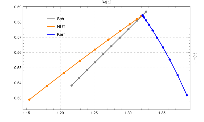
(a) Scalar field without mass

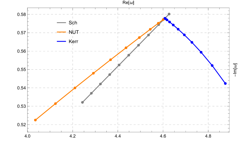
(b) Spinor field without mass

Figure 2: Phase diagram of QNFs under a massless field perturbation, where $M=1/2$, $N=0,0.038,0.076,\cdots,0.38$ (Taub-NUT BHs), and $a=0,0.0405,0.0810,\cdots,0.405$ (Kerr BHs) are set.

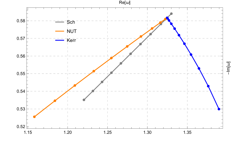
(a) Scalar field with mass

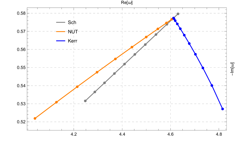
(b) Spinor field with mass

Figure 3: Phase diagram of QNFs under a massive field perturbation, where $m_{0}=m_{e}=0.2$, $M=1/2$, $N=0,0.038,0.076,\cdots,0.38$ (Taub-NUT BHs), and $a=0,0.0405,0.0810,\cdots,0.405$ (Kerr BHs) are set.

The gray lines represent the variation of the QNFs of Schwarzschild BHs when the mass parameter $M$ varies from 0.498 to 0.503, where $11$ equidistant points are selected, i.e., the step size is taken to be $0.005$. The orange curves depict the QNFs of Taub-NUT BHs when the NUT charge varies but the mass is fixed to be $M=1/2$. Here, we assume that $N$ is continuous, and that $11$ equidistant points are chosen between $N=0$ and $N=0.38$, i.e., the step size is taken to be $0.038$. The blue curves represent the variation of QNFs of Kerr BHs with respect to the rotation parameter $a$ under a fixed mass $M=1/2$, where $11$ equidistant points are taken from $a=0$ to $a=0.405$, i.e., the step size is taken to be $0.0405$. To sum up, Figs. 2(a) and 3(a) display the results for a massless and massive scalar field perturbations, respectively, and Figs. 2(b) and 3(b) show the results for a massless and massive spinor field perturbations, respectively. We can see that Figs. 2 and 3 are consistent with Fig. 1 obtained earlier through the light ring/QNMs correspondence.

In the relationships among the QNFs of the three BHs in different multipole number $l$ and overtine number $n$, we also find the linear relations of real parts between any two of the three BHs, and the linear relations of imaginary parts between any two of the three BHs, where Fig. 4 and Fig. 5 correspond to massless and massive scalar field perturbations, respectively, and Fig. 6 and Fig. 7 correspond to massless and massive spinor field perturbations, respectively. The notation “Sch vs Taub” means that the horizontal axis denotes the real (imaginary) parts of QNFs of Schwarzschild BHs, and the vertical axis stands for that of QNFs of Taub-NUT BHs. The similar meanings are taken for the others, i.e., “Sch vs Kerr” and “Kerr vs Taub”.

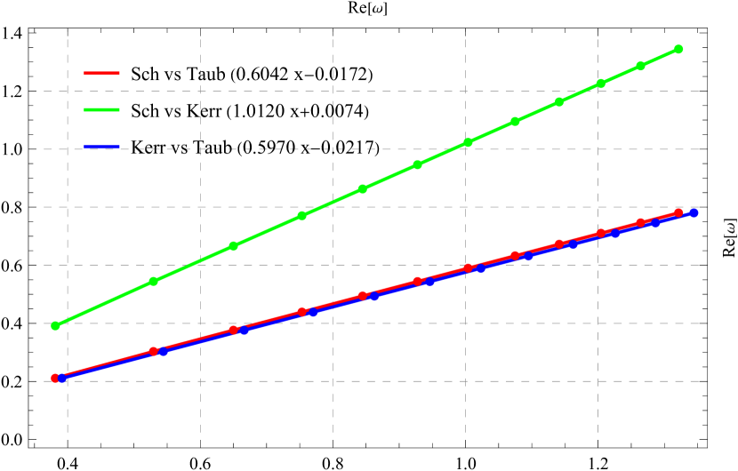
(a) Real parts, $n=1$ and $\lambda=1,2,\cdots,12$.

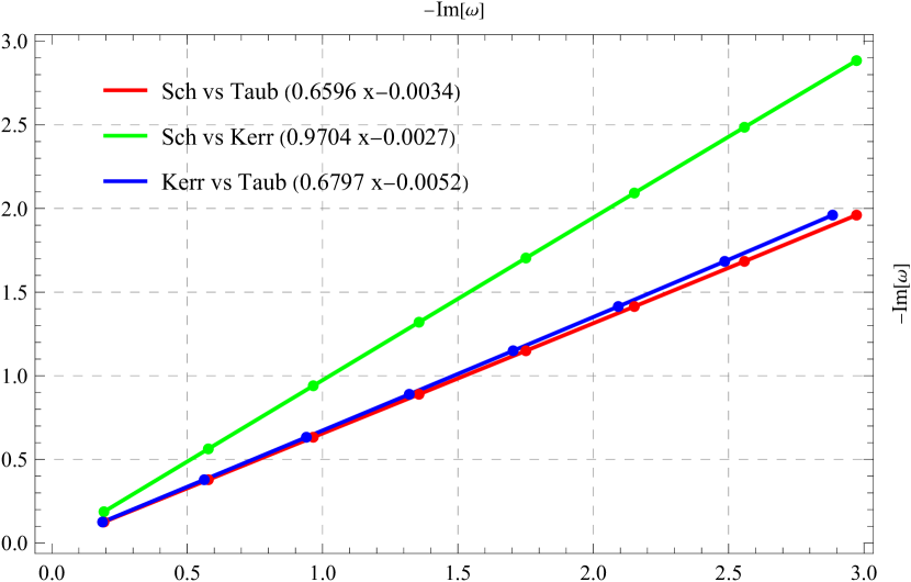
(b) Imaginary parts, $l=10$ and $n=0,1,\cdots,7$.

Figure 4: QNFs of Schwarzschild, Kerr, and Taub-NUT BHs under a massless scalar field perturbation. The rotation parameter $a=0.25$ for Kerr BHs and the NUT charge $N=1$ for Taub-NUT BHs are set. Moreover, $m=0$ is set for Kerr BHs.

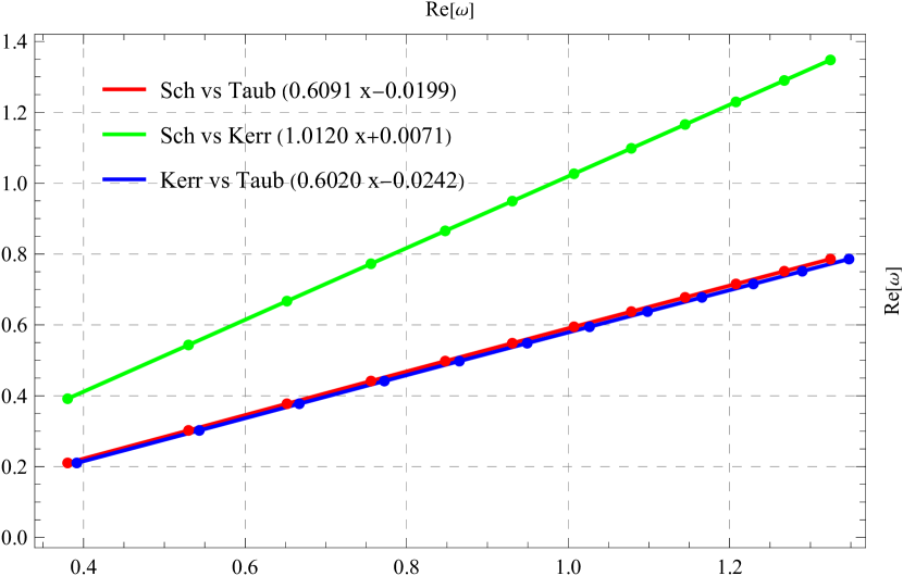
(a) Real parts, $n=1$ and $\lambda=1,2,\cdots,12$.

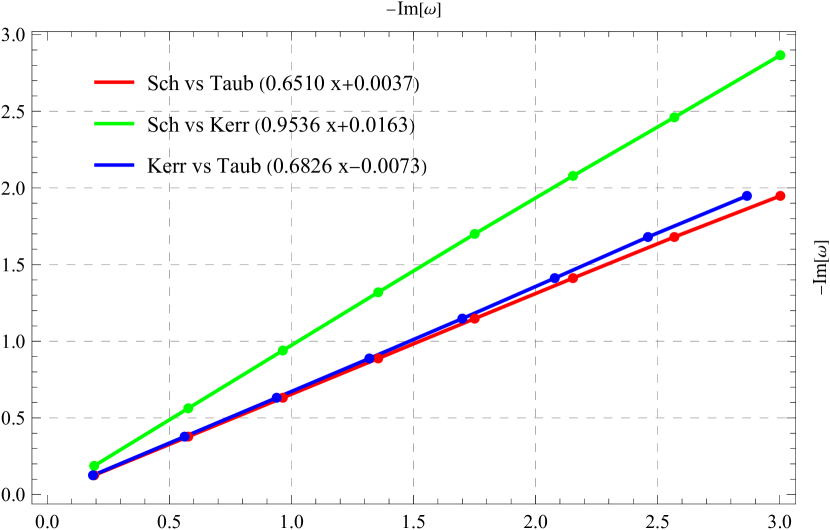
(b) Imaginary parts, $l=10$ and $n=0,1,\cdots,7$.

Figure 5: QNFs of Schwarzschild, Kerr, and Taub-NUT BHs under a massive scalar field perturbation. The mass $m_{0}=0.2$, the rotation parameter $a=0.25$ for Kerr BHs, and the NUT charge $N=1$ for Taub-NUT BHs are set. Moreover, $m=0$ is set for Kerr BHs.

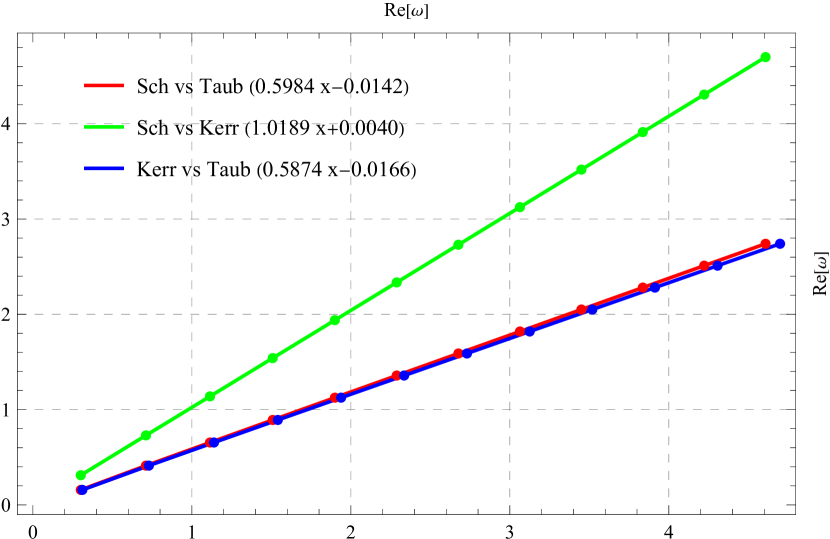
(a) Real parts, $n=1$ and $\lambda_{-}=1,2,\cdots,12$.

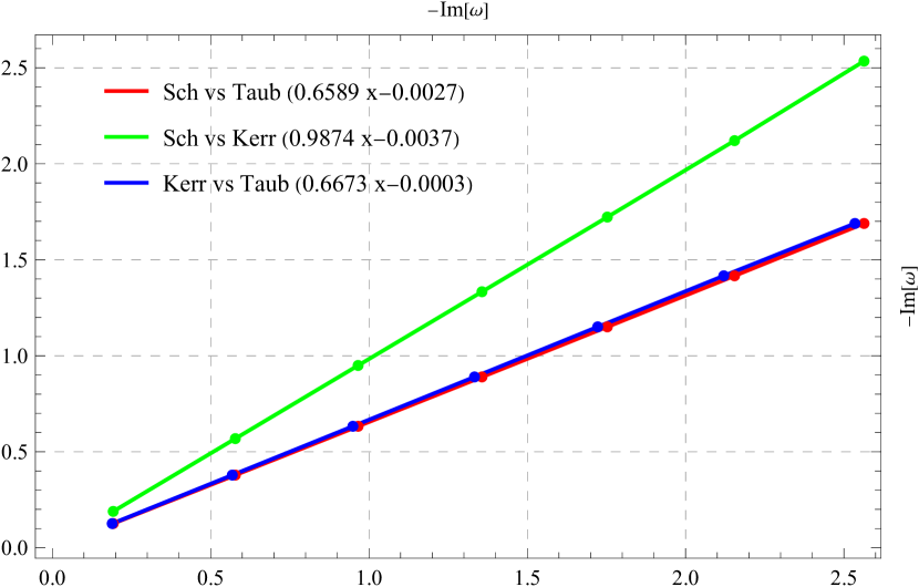
(b) Imaginary parts, $l=10$ and $n=0,1,\cdots,6$.

Figure 6: QNFs of Schwarzschild, Kerr, and Taub-NUT BHs under the massless spinor field-$P_{-\frac{1}{2}}$ perturbation. The rotation parameter $a=0.25$ for Kerr BHs and the NUT charge $N=1$ for Taub-NUT BHs are set. Moreover, $m=0$ is set for Kerr BHs.

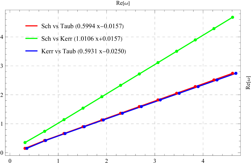
(a) Real parts, $n=1$ and $\lambda_{-}=1,2,\cdots,12$.

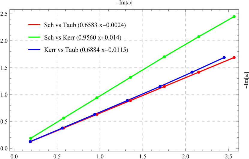
(b) Imaginary parts, $l=10$ and $n=0,1,\cdots,6$.

Figure 7: QNFs of Schwarzschild, Kerr, and Taub-NUT BHs under the massive spinor field-$P_{-\frac{1}{2}}$ perturbation. The mass $m_{e}=0.1$, the rotation parameter $a=0.25$ for Kerr BHs, and the NUT charge $N=1$ for Taub-NUT BHs are set. Moreover, $m=0$ is set for Kerr BHs.

Fig. 4(a) shows the variation of QNFs’ real parts with respect to the separation constant$\lambda$ that runs from $1$ to $12$, and Fig. 4(b) shows the variation of QNFs’ imaginary parts with respect to the overtone number $n$ that runs from $0$ to $7$. Moreover, Fig. 5 depicts the situation under a massive scalar field perturbation, Fig. 6 illustrates the situation under a massless spinor field perturbation, and Fig. 7 gives the situation under a massive spinor field perturbation. The points in these figures represent the numerical results and are dealt with by linear fitting, where the corresponding linear functions are indicated in the figures. In addition, we note that the two components of spinor fields, $P_{\pm\frac{1}{2}}$, have the same spectra because of the symmetry. Hence, we only focus on $P_{-\frac{1}{2}}$ in Figs. 6 and 7.

From Figs. 4, 5, 6 and 7, we observe that the real parts, $\real(\omega)$, increase when the separation constant $\lambda$ or $\lambda_{-}$ grows, and the minus imaginary parts, $-\imaginary(\omega)$, also increase when the overtone number $n$ becomes large, as we predict in Sec. 3.4 in terms of the light ring/QNMs correspondence. Specifically, when we compare Kerr BHs with Schwarzschild BHs, we find that the former’s rotation parameter $a$ as a variable of the NJA produces the effects of increasing oscillation frequencies (the real parts of QNFs) but decreasing damping rates (the imaginary parts of QNFs); when we compare Taub-NUT BHs with Schwarzschild BHs, we find that the former’s NUT charge $N$ as a variable of the NJA produces the effects of weakening both the oscillation frequencies and damping rates. In addition, the fitting results, i.e., the slopes of fitting lines are consistent with the the analytical estimations, Eqs. (28), (29), and (30).

7 Conclusions

It is an interesting topic to examine the physical reasons behind the mathematical connections established by the NJA, as mentioned in Refs. [15, 46]. In this paper, we explore the connections through a dynamical behavior of BHs, i.e., the QNFs of BHs under field perturbations. We find that these relationships are more than just mathematical operations and believe that the physical manifestations will be verified by future observations of GWs.

We notice that the rotation parameter $a$ increases the oscillation frequencies, while the NUT charge $N$ decreases them in Kerr-Taub-NUT BHs. However, both $a$ and $N$ decrease the damping rates, suggesting that the NJA has a dampening effect on wave oscillations. Furthermore, we obtain the linear relations in real parts of QNFs between any two of Schwarzschild, Kerr, and Taub-NUT BHs, and also in the imaginary parts of QNFs between any two of the three BHs, which holds even beyond the eikonal limit. This implies that NJA has the ability to categorize BHs. In other words, all BHs generated with the same seed using various NJAs can be seen as belonging to a single NJA class.

The QNFs of Schwarzschild BHs divide the NJA operation into two phases in the complex frequency plane, which is referred to as the Kerr and Taub-NUT phases. Interestingly, the QNFs exhibit several similar characteristics in these two phases. Firstly, they vary monotonically with respect to the parameter $a$ or $N$, which is distinct from the vortex shape observed [47, 48] in RN or Einstein-Maxwell dilaton-axion BHs. Secondly, the damping rates vanish when the parameters $a$ and $N$ approach infinity. Lastly, the QNFs of Kerr and Taub-NUT BHs never cross the barrier established by the QNFs of Schwarzschild BHs owing to the topological protection [26].

We believe that the NJA goes beyond a mere mathematical procedure for generating additional solutions to Einstein’s equations. We assert that the NJA carries profound physical implications that would be observed empirically. This serves as the primary motivation of our present work, aiming to reveal the relationships that hide behind the QNFs of BHs connected by the NJA. It is worth mentioning that such relationships may also be investigated through alternative means, such as the study of perturbation waveforms, which is one of our proceeding works.

Appendix A Recurrence relations and coefficients

In this appendix, we provide a compilation of the coefficients used in the recurrence relations for scalar and spinor field perturbations, where both the massless and massive cases are considered. These coefficients have been utilized in the calculation of the QNFs in Sec. 6. For the details of derivations, see the review article [6].

A.1 Coefficients in recurrence relations for a massless scalar field perturbation

The hoirzon is

$$r_{\rm H}=\frac{1}{2}\left(\sqrt{4N^{2}+1}+1\right),$$ (73)

where we have utilized the value of $M$ as $1/2$ in this and subsequent formulas.

$$\alpha_{n}=-(n+1)(n-2\mathrm{i}r_{\rm H}\omega+1),$$ (74)

$$\beta_{n}=\lambda+3n^{2}-10\mathrm{i}nr_{\rm H}\omega-8r_{\rm H}^{2}\omega^{2}-2\mathrm{i}r_{\rm H}\omega,$$ (75)

$$\gamma_{n}=-\lambda-3n^{2}+2\mathrm{i}n(5r_{\rm H}+1)\omega+6n+8r_{\rm H}^{2}\omega^{2}+4r_{\rm H}\omega^{2}-12\mathrm{i}r_{\rm H}\omega-3,$$ (76)

$$\delta_{n}=(n-2\mathrm{i}\omega-2)(n-2\mathrm{i}r_{\rm H}\omega-2).$$ (77)

A.2 Coefficients in recurrence relations for a massive scalar field perturbation

In order to write the following formulas more concise, we use $m$ instead of $m_{0}$ to denote the mass of massive scalar fields.

$$\alpha_{n}=-\mathrm{i}4(n+1)\chi^{3}(n-2\mathrm{i}r_{\rm H}\omega+1),$$ (78)

$$\begin{split}\beta_{n}=&-2\chi^{2}\Big{\{}-2\mathrm{i}\chi\left(\lambda+3n^{2}\right)-2\omega^{2}\left(2n-4\mathrm{i}r_{\rm H}^{2}\chi+1\right)+m^{2}[2n-2\mathrm{i}r_{\rm H}(r_{\rm H}\chi+\omega)+1]\\ &-2(2n+1)(2r_{\rm H}-1)\chi^{2}+4\mathrm{i}r_{\rm H}\chi\omega[(2r_{\rm H}-1)\chi+3\mathrm{i}n]+4\mathrm{i}r_{\rm H}\omega^{3}\Big{\}},\end{split}$$ (79)

$$\begin{split}\gamma_{n}=&m^{4}\left[-8n+\mathrm{i}\left(4r_{\rm H}^{2}\chi+8r_{\rm H}\omega+\chi-6\mathrm{i}\right)\right]+2m^{2}\Big{\{}2\chi\Big{[}\mathrm{i}\left(\lambda+3(n-1)^{2}\right)+6(n-1)r_{\rm H}\omega\\ &-\mathrm{i}r_{\rm H}(5r_{\rm H}+2)\omega^{2}\Big{]}+2(2r_{\rm H}-1)\chi^{2}(2n-2\mathrm{i}r_{\rm H}\omega-3)+3\omega^{2}(4n-4\mathrm{i}r_{\rm H}\omega-3)\Big{\}}\\ &+4\omega^{2}\Big{\{}\chi\Big{[}-\mathrm{i}\left(\lambda+3(n-1)^{2}\right)-6(n-1)r_{\rm H}\omega+2\mathrm{i}r_{\rm H}(2r_{\rm H}+1)\omega^{2}\Big{]}\\ &+(2r_{\rm H}-1)\chi^{2}(-2n+2\mathrm{i}r_{\rm H}\omega+3)+\omega^{2}(-4n+4\mathrm{i}r_{\rm H}\omega+3)\Big{\}},\end{split}$$ (80)

$$\begin{split}\delta_{n}=&m^{4}[4n-\mathrm{i}(4r_{\rm H}\omega+\chi-8\mathrm{i})]+4m^{2}\Big{[}\omega^{2}(-3n+2\mathrm{i}r_{\rm H}\chi+6)-2(n-2)r_{\rm H}\chi\omega-\mathrm{i}(n-2)^{2}\chi\\ &+3\mathrm{i}r_{\rm H}\omega^{3}\Big{]}+4\chi\omega^{2}\left(2(n-2)r_{\rm H}\omega+\mathrm{i}(n-2)^{2}-2\mathrm{i}r_{\rm H}\omega^{2}\right)+8\omega^{4}(n-ir_{\rm H}\omega-2).\end{split}$$ (81)

Here we have

$$\chi=\sqrt{\omega^{2}-m^{2}}.$$ (82)

A.3 Coefficients in recurrence relations for a massless spinor field perturbation

$$h=\sqrt{4N^{2}+1},\qquad\sigma=\frac{1}{2}(h+1)k.$$ (83)

$$\alpha_{n}=[(h+1)k-2\mathrm{i}(n+1)-2\sigma](hk+k+2\mathrm{i}n+2\sigma+3\mathrm{i}),$$ (84)

$$\beta_{n}=2(h+1)^{2}k^{2}+4(h+1)k(2\mathrm{i}n+2\sigma+\mathrm{i})-4\lambda^{2}+8\mathrm{i}(2n+1)\sigma-8n(n+1)+8\sigma^{2}-2,$$ (85)

$$\gamma_{n}=[(h-3)k-2\mathrm{i}n-2\sigma](hk+k+2\mathrm{i}n+2\sigma-\mathrm{i}).$$ (86)

A.4 Coefficients in recurrence relations for a massive spinor field perturbation

In order to write the following formulas more concise, we use $m$ instead of $m_{e}$ to denote the mass of massive spinor fields.

$$\alpha_{n}=-2(n+1)(mr_{\rm H}-\mathrm{i}\lambda)\chi^{2}(2n-4\mathrm{i}r_{\rm H}\omega+3)$$ (87)

$$\begin{split}\beta_{n}=&-4r_{\rm H}^{3}m^{5}+4\mathrm{i}r_{\rm H}^{2}\lambda m^{4}+\big{[}20\omega^{2}r_{\rm H}^{3}+20\mathrm{i}\omega r_{\rm H}^{2}-2\left(2\lambda^{2}+2\mathrm{i}n\chi+4\mathrm{i}\omega+3\right)r_{\rm H}+2\big{]}m^{3}\\ &+2\lambda\left(2\mathrm{i}\lambda^{2}-10\mathrm{i}r_{\rm H}^{2}\omega^{2}+\mathrm{i}+2n(4r_{\rm H}-1)\chi+2r_{\rm H}\omega\right)m^{2}\\ &+\big{\{}-16\omega\left(\chi^{3}+\omega^{3}\right)r_{\rm H}^{3}+4[(-3\mathrm{i}+\omega)\chi^{3}-\omega^{3}\chi-5\mathrm{i}\omega^{3}]r_{\rm H}^{2}+[3\mathrm{i}\chi^{3}-3\mathrm{i}\omega^{2}\chi\\ &+2\omega^{2}\left(2\lambda^{2}+4\mathrm{i}\omega+3\right)]r_{\rm H}+4n^{2}(r_{\rm H}+1)\chi^{2}-2\omega^{2}+2n\chi^{2}[-4\mathrm{i}(2\chi+\omega)r_{\rm H}^{2}\\ &+(7-4\mathrm{i}\omega)r_{\rm H}-1]\big{\}}m-\mathrm{i}\lambda\big{\{}-[(4r_{\rm H}-1)(3\mathrm{i}+4r_{\rm H}\omega)\chi^{3}]+12n^{2}\chi^{2}-\omega^{2}(3\mathrm{i}+4r_{\rm H}\omega)\chi\\ &+2n[\chi(5-12\mathrm{i}r_{\rm H}\omega)-8\mathrm{i}r_{\rm H}\omega^{2}]\chi+2\omega^{2}\left(2\lambda^{2}-8r_{\rm H}^{2}\omega^{2}-2\mathrm{i}r_{\rm H}\omega+1\right)\big{\}}\end{split}$$ (88)

$$\begin{split}\gamma_{n}=&\left(-4r_{\rm H}^{3}+4r_{\rm H}^{2}+r_{\rm H}\right)m^{5}-\mathrm{i}\left(4\lambda r_{\rm H}^{2}+\lambda\right)m^{4}+2\big{\{}10\omega^{2}r_{\rm H}^{3}-2\omega(3\mathrm{i}+7\omega)r_{\rm H}^{2}\\ &+[-2\lambda^{2}-12\mathrm{i}(n-1)\chi+\mathrm{i}\omega+2]r_{\rm H}+2\lambda^{2}+2\mathrm{i}(n-1)\chi\big{\}}m^{3}+2\lambda[-2\mathrm{i}\lambda^{2}\\ &+10\mathrm{i}r_{\rm H}^{2}\omega^{2}-2\mathrm{i}-8(n-1)r_{\rm H}\chi+3\omega+2r_{\rm H}\omega(2\mathrm{i}\omega-5)]m^{2}+\big{\{}[-16\omega r_{\rm H}^{3}\\ &+4(3\mathrm{i}-4\mathrm{i}n+6\omega)r_{\rm H}^{2}+(10\mathrm{i}-4\omega)r_{\rm H}-\mathrm{i}]\chi^{3}+2(n-1)[-4\mathrm{i}\omega r_{\rm H}^{2}+(8\mathrm{i}\omega-5)r_{\rm H}\\ &+2n(r_{\rm H}-2)+2]\chi^{2}+\omega^{2}[\mathrm{i}+4r_{\rm H}(-5\mathrm{i}+6\mathrm{i}n+\omega)]\chi-2\omega^{2}[8\omega^{2}r_{\rm H}^{3}-6\omega(\mathrm{i}+2\omega)r_{\rm H}^{2}\\ &+\left(-2\lambda^{2}+\mathrm{i}\omega+2\right)r_{\rm H}+2\lambda^{2}]\big{\}}m+2\lambda\big{\{}2\left(-4\mathrm{i}\omega r_{\rm H}^{2}+r_{\rm H}+1\right)\chi^{3}\\ &+(n-1)(\mathrm{i}+6\mathrm{i}n+12r_{\rm H}\omega)\chi^{2}+\omega^{2}(n(8r_{\rm H}+4)+r_{\rm H}(-4\mathrm{i}\omega-8)-1)\chi\\ &+\omega^{2}\left(2\mathrm{i}\lambda^{2}-4\mathrm{i}r_{\rm H}(2r_{\rm H}+1)\omega^{2}+2\mathrm{i}+(10r_{\rm H}-3)\omega\right)\big{\}}\end{split}$$ (89)

$$\begin{split}\delta_{n}=&[m(r_{\rm H}-1)+i\lambda]\big{\{}m^{4}+[-8r_{\rm H}\omega^{2}+2\mathrm{i}\omega-8\mathrm{i}r_{\rm H}\omega-4\mathrm{i}(n-2)\chi+2]m^{2}\\ &+\chi^{3}(3\mathrm{i}+4r_{\rm H}\omega)+\chi\omega^{2}(-13\mathrm{i}+8\mathrm{i}n+4r_{\rm H}\omega)-2(n-2)\chi^{2}(2n-4\mathrm{i}r_{\rm H}\omega-1)\\ &+2\omega^{2}\left(4r_{\rm H}\omega^{2}+i(4r_{\rm H}-1)\omega-1\right)\big{\}}\end{split}$$ (90)

References

- [1] LIGO Scientific, Virgo Collaboration, B. P. Abbott et al., “Observation of Gravitational Waves from a Binary Black Hole Merger,” Phys. Rev. Lett. 116 no. 6, (2016) 061102, arXiv:1602.03837 [gr-qc].
- [2] LIGO Scientific, Virgo Collaboration, B. P. Abbott et al., “Tests of general relativity with GW150914,” Phys. Rev. Lett. 116 no. 22, (2016) 221101, arXiv:1602.03841 [gr-qc]. [Erratum: Phys.Rev.Lett. 121, 129902 (2018)].
- [3] A. Neronov, “Introduction to multi-messenger astronomy,” J. Phys. Conf. Ser. 1263 no. 1, (2019) 012001, arXiv:1907.07392 [astro-ph.HE].
- [4] P. Mészáros, D. B. Fox, C. Hanna, and K. Murase, “Multi-Messenger Astrophysics,” Nature Rev. Phys. 1 (2019) 585–599, arXiv:1906.10212 [astro-ph.HE].
- [5] F. Pretorius, “Evolution of binary black hole spacetimes,” Phys. Rev. Lett. 95 (2005) 121101, arXiv:gr-qc/0507014.
- [6] R. A. Konoplya and A. Zhidenko, “Quasinormal modes of black holes: From astrophysics to string theory,” Rev. Mod. Phys. 83 (2011) 793–836, arXiv:1102.4014 [gr-qc].
- [7] E. T. Newman and A. I. Janis, “Note on the Kerr spinning particle metric,” J. Math. Phys. 6 (1965) 915–917.
- [8] C. Bambi and L. Modesto, “Rotating regular black holes,” Phys. Lett. B 721 (2013) 329–334, arXiv:1302.6075 [gr-qc].
- [9] B. Toshmatov, B. Ahmedov, A. Abdujabbarov, and Z. Stuchlik, “Rotating Regular Black Hole Solution,” Phys. Rev. D 89 no. 10, (2014) 104017, arXiv:1404.6443 [gr-qc].
- [10] M. Azreg-Aïnou, “Generating rotating regular black hole solutions without complexification,” Phys. Rev. D 90 no. 6, (2014) 064041, arXiv:1405.2569 [gr-qc].
- [11] L. Modesto and P. Nicolini, “Charged rotating noncommutative black holes,” Phys. Rev. D 82 (2010) 104035, arXiv:1005.5605 [gr-qc].
- [12] S. Brahma, C.-Y. Chen, and D.-h. Yeom, “Testing Loop Quantum Gravity from Observational Consequences of Nonsingular Rotating Black Holes,” Phys. Rev. Lett. 126 no. 18, (2021) 181301, arXiv:2012.08785 [gr-qc].
- [13] R. Torres, “Regular Rotating Black Holes: A Review,” arXiv:2208.12713 [gr-qc].
- [14] C. Lan, H. Yang, Y. Guo, and Y.-G. Miao, “Regular black holes: A short topic review,” Int. J. Theor. Phys. 62 (2023) 202, arXiv:2303.11696 [gr-qc].
- [15] N. Arkani-Hamed, Y.-t. Huang, and D. O’Connell, “Kerr black holes as elementary particles,” JHEP 01 (2020) 046, arXiv:1906.10100 [hep-th].
- [16] C. J. Talbot, “Newman-Penrose approach to twisting degenerate metrics,” Commun. Math. Phys. 13 no. 1, (1969) 45–61.
- [17] A. Luna, R. Monteiro, D. O’Connell, and C. D. White, “The classical double copy for Taub–NUT spacetime,” Phys. Lett. B 750 (2015) 272–277, arXiv:1507.01869 [hep-th].
- [18] C. Lan and Y.-F. Wang, “Singularities of regular black holes and the monodromy method for asymptotic quasinormal modes*,” Chin. Phys. C 47 no. 2, (2023) 025103, arXiv:2205.05935 [gr-qc].
- [19] J. G. Miller, “Global analysis of the Kerr-Taub-NUT metric,” Journal of Mathematical Physics 14 no. 4, (1973) 486–494.
- [20] S.-J. Yang, J. Chen, J.-J. Wan, S.-W. Wei, and Y.-X. Liu, “Weak cosmic censorship conjecture for a Kerr-Taub-NUT black hole with a test scalar field and particle,” Phys. Rev. D 101 no. 6, (2020) 064048, arXiv:2001.03106 [gr-qc].
- [21] E. Zakhary and C. B. G. Mcintosh, “A Complete Set of Riemann Invariants,” Gen. Rel. and Grav. 29 (1997) 539–581.
- [22] C. W. Misner, K. S. Thorne, and J. A. Wheeler, Gravitation. W. H. Freeman, San Francisco, 1973.
- [23] V. Cardoso, A. S. Miranda, E. Berti, H. Witek, and V. T. Zanchin, “Geodesic stability, Lyapunov exponents and quasinormal modes,” Phys. Rev. D 79 no. 6, (2009) 064016, arXiv:0812.1806 [hep-th].
- [24] C. Chakraborty, “Inner-most stable circular orbits in extremal and non-extremal Kerr-Taub-NUT spacetimes,” Eur. Phys. J. C 74 no. 99, (2014) 2759, arXiv:1307.4698 [gr-qc].
- [25] P. Pradhan, “Circular geodesics in the Kerr–Newman–Taub–NUT spacetime,” Class. Quant. Grav. 32 no. 16, (2015) 165001, arXiv:1402.0089 [gr-qc].
- [26] A. Borde, “Regular black holes and topology change,” Phys. Rev. D 55 (1997) 7615–7617, arXiv:gr-qc/9612057.
- [27] S. A. Teukolsky, “Rotating black holes - separable wave equations for gravitational and electromagnetic perturbations,” Phys. Rev. Lett. 29 (1972) 1114–1118.
- [28] S. A. Teukolsky, “Perturbations of a rotating black hole. 1. Fundamental equations for gravitational electromagnetic and neutrino field perturbations,” Astrophys. J. 185 (1973) 635–647.
- [29] S.-J. Yang, W.-D. Guo, S.-W. Wei, and Y.-X. Liu, “Thermodynamics and weak cosmic censorship conjecture for a Kerr-Newman Taub-NUT black hole,” arXiv:2306.05266 [gr-qc].
- [30] S. Chandrasekhar and S. Detweller, The Mathematical Theory of Black Holes. Proc. R. Soc. Lond., 1975.
- [31] P. Collas and D. Klein, The Dirac Equation in Curved Spacetime: A Guide for Calculations. SpringerBriefs in Physics. Springer, 2019. arXiv:1809.02764 [gr-qc].
- [32] J.-l. Jing, “Dirac quasinormal modes of Schwarzschild black hole,” Phys. Rev. D 71 (2005) 124006, arXiv:gr-qc/0502023.
- [33] S. Chandrasekhar, “The Solution of Dirac’s Equation in Kerr Geometry,” Proc. Roy. Soc. Lond. A 349 (1976) 571–575.
- [34] D. N. Page, “Dirac Equation Around a Charged, Rotating Black Hole,” Phys. Rev. D 14 (1976) 1509–1510.
- [35] E. Seidel, “A Comment on the Eigenvalues of Spin Weighted Spheroidal Functions,” Class. Quant. Grav. 6 (1989) 1057.
- [36] E. Berti, V. Cardoso, and M. Casals, “Eigenvalues and eigenfunctions of spin-weighted spheroidal harmonics in four and higher dimensions,” Phys. Rev. D 73 (2006) 024013, arXiv:gr-qc/0511111. [Erratum: Phys.Rev.D 73, 109902 (2006)].
- [37] “NIST Digital Library of Mathematical Functions.” Http://dlmf.nist.gov/, release 1.1.7 of 2022-10-15. http://dlmf.nist.gov/. F. W. J. Olver, A. B. Olde Daalhuis, D. W. Lozier, B. I. Schneider, R. F. Boisvert, C. W. Clark, B. R. Miller, B. V. Saunders, H. S. Cohl, and M. A. McClain, eds.
- [38] E. W. Leaver, “An Analytic representation for the quasi normal modes of Kerr black holes,” Proc. Roy. Soc. Lond. A 402 (1985) 285–298.
- [39] H.-P. Nollert, “Quasinormal modes of schwarzschild black holes: The determination of quasinormal frequencies with very large imaginary parts,” Phys. Rev. D 47 (1993) 5253–5258.
- [40] E. W. Leaver, “Quasinormal modes of Reissner-Nordstrom black holes,” Phys. Rev. D 41 (1990) 2986–2997.
- [41] R. A. Konoplya and A. V. Zhidenko, “Decay of massive scalar field in a Schwarzschild background,” Phys. Lett. B 609 (2005) 377–384, arXiv:gr-qc/0411059.
- [42] R. A. Konoplya and A. Zhidenko, “Stability and quasinormal modes of the massive scalar field around Kerr black holes,” Phys. Rev. D 73 (2006) 124040, arXiv:gr-qc/0605013.
- [43] J.-l. Jing and Q.-y. Pan, “Dirac quasinormal frequencies of the Kerr-Newman black hole,” Nucl. Phys. B 728 (2005) 109–120, arXiv:gr-qc/0506098.
- [44] R. A. Konoplya and A. Zhidenko, “Quasinormal modes of massive fermions in Kerr spacetime: Long-lived modes and the fine structure,” Phys. Rev. D 97 no. 8, (2018) 084034, arXiv:1712.06667 [gr-qc].
- [45] F. Cooper, A. Khare, and U. Sukhatme, “Supersymmetry and quantum mechanics,” Phys. Rept. 251 (1995) 267–385, arXiv:hep-th/9405029.
- [46] W. T. Emond, Y.-T. Huang, U. Kol, N. Moynihan, and D. O’Connell, “Amplitudes from Coulomb to Kerr-Taub-NUT,” JHEP 05 (2022) 055, arXiv:2010.07861 [hep-th].
- [47] J. Jing and Q. Pan, “Quasinormal modes and second order thermodynamic phase transition for Reissner-Nordstrom black hole,” Phys. Lett. B 660 (2008) 13–18, arXiv:0802.0043 [gr-qc].
- [48] Q.-Y. Pan and J.-L. Jing, “Quasinormal frequencies and thermodynamic instabilities for the stationary axisymmetric Einstein-Maxwell dilaton-axion black hole,” JHEP 01 (2007) 044.