Consistency Models for Scalable and Fast Simulation-Based Inference

Abstract

Simulation-based inference (SBI) is constantly in search of more expressive algorithms for accurately inferring the parameters of complex models from noisy data. We present consistency models for neural posterior estimation (CMPE), a new free-form conditional sampler for scalable, fast, and amortized SBI with generative neural networks. CMPE combines the advantages of normalizing flows and flow matching methods into a single generative architecture: It essentially distills a continuous probability flow and enables rapid few-shot inference with an unconstrained architecture that can be tailored to the structure of the estimation problem. Our empirical evaluation demonstrates that CMPE not only outperforms current state-of-the-art algorithms on three hard low-dimensional problems, but also achieves competitive performance in a high-dimensional Bayesian denoising experiment and in estimating a computationally demanding multi-scale model of tumor spheroid growth.

1 Introduction

Computer simulations play a fundamental role across countless scientific disciplines, ranging from physics to biology, and from climate science to economics (Lavin et al., 2021). Simulation programs generate observables $\mathbf{x}\in\mathcal{X}$ as a function of unknown parameters $\boldsymbol{\theta}\in\Theta$ and latent program states $\boldsymbol{\xi}\in\Xi$ (Cranmer et al., 2020). This forward problem is typically well-understood through mechanistic models or scientific theories. The inverse problem, however, is much harder, and forms the crux of Bayesian (probabilistic) inference: Reasoning about the unknowns $\boldsymbol{\theta}$ based on observables $\mathbf{x}$. Bayes’ theorem captures the full distribution of plausible parameters $\boldsymbol{\theta}$ conditional on the observed data $\mathbf{x}$ as $p(\boldsymbol{\theta}\,|\,\mathbf{x})\propto p(\boldsymbol{\theta})\,p(\mathbf{x}\,|\,\boldsymbol{\theta})$ given a prior $p(\boldsymbol{\theta})$. While generating synthetic data from the simulation program is possible (albeit potentially slow), the likelihood density $p(\mathbf{x}\,|\,\boldsymbol{\theta})$ is generally not explicitly available. Instead, it is only implicitly defined through a high-dimensional integral over all possible program execution paths (Cranmer et al., 2020), $p(\mathbf{x}\,|\,\boldsymbol{\theta})=\int p(\mathbf{x}\,|\,\boldsymbol{\theta},\boldsymbol{\xi})\mathrm{d}\boldsymbol{\xi}$. A new era of simulation science (Cranmer et al., 2020; Lavin et al., 2021) aims to address this challenging setting with remarkable success across various application domains (Butter et al., 2022; Radev et al., 2021b; Gonçalves et al., 2020; Shiono, 2021; Bieringer et al., 2021; von Krause et al., 2022; Ghaderi-Kangavari et al., 2023; Boelts et al., 2023). These advances in simulation-based inference (SBI) are co-developing with rapid progress in conditional generative modeling.

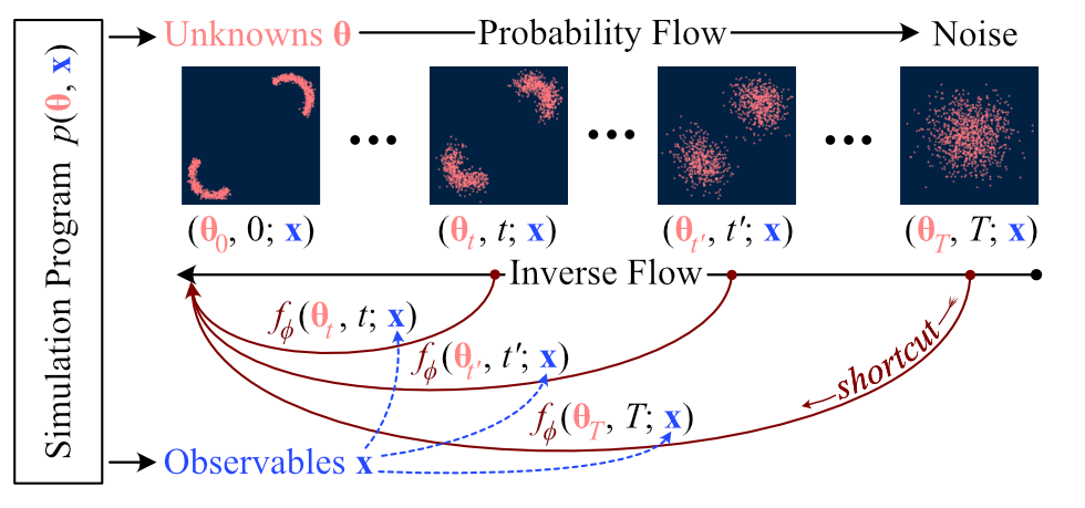
Figure 1: Inverting a probability flow on a target vector $\boldsymbol{\theta}$ forms the core of modern denoising models. Consistency models (Song et al., 2023) learn a shortcut $f_{\phi}$ that maps any point on the trajectory directly to the origin $\boldsymbol{\theta}_{0}$. We extend consistency models by conditioning on observable data $\mathbf{x}$ and infer statistical model parameters $\boldsymbol{\theta}$ as the target vector. As a consequence, the probability distribution over the origin $p({\color[rgb]{1,0.5234375,0.5234375}\boldsymbol{\theta}_{0}}\,|\,{\color[rgb]{0,0,1}\mathbf{x}})$ is the Bayesian posterior by definition. We call this approach consistency model posterior estimation (CMPE), which is a new amortized method for scalable and fast simulation-based inference.

Currently, advancements in generative neural networks primarily manifest in remarkable performance on generating images (Goodfellow et al., 2014), videos (Vondrick et al., 2016), and audio (Engel et al., 2020).

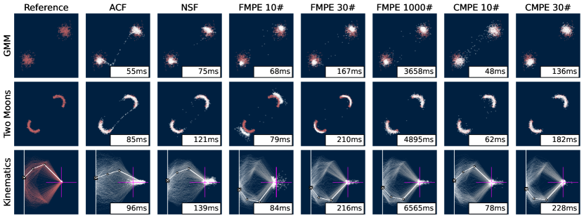
Figure 2: Experiments 1–3. 1000 posterior draws for one unseen test instance per task, as well as sampling time in milliseconds. All amortized approximators were trained on $M=1024$ simulations. The bottom row shows the posterior predictive distribution in the kinematics task, and the pink cross-hair indicates the true end location $\mathbf{x}$ of the robot arm. Across all benchmarks, CMPE yields the best trade-off between fast sampling speed and high accuracy. ACF: affine coupling flow, NSF: neural spline flow, FMPE: flow matching posterior estimation, CMPE: consistency model posterior estimation (ours), K# denotes $K$ sampling steps.

Within the class of generative models, score-based diffusion models (Song et al., 2021; Rombach et al., 2022; Ho et al., 2020; Batzolis et al., 2021) have recently attracted significant attention due to their sublime performance as realistic generators. Diffusion models are strikingly flexible but require a multi-step sampling phase to denoise samples (Song et al., 2021). To address this fundamental shortcoming, Song et al. (2023) have proposed consistency models, which are trained to perform few-step generation by design. In this paper, we port consistency models to simulation-based inference (see Figure 1) to achieve an unprecedented combination of both scalable and fast neural posterior estimation. Our main contributions are:

1. We adapt conditional consistency models to simulation-based Bayesian inference and propose consistency model posterior estimation (CMPE);

2. We illustrate the fundamental advantages of consistency models for simulation-based inference: expressive free-form architectures and fast inference;

3. We demonstrate that CMPE outperforms both normalizing flows and flow matching on three benchmark experiments (see Figure 2 above), high-dimensional Bayesian denoising, and a tumor spheroid model.

2 Preliminaries

This section briefly recaps simulation-based inference, as well as score-based diffusion models and consistency models. Acquainted readers can fast-forward to Section 3.

2.1 Simulation-Based Inference (SBI)

The defining property of SBI methods is that they purely build on the ability to sample from the data-generating process – as opposed to likelihood-based methods which rely on evaluating some likelihood function of interest. Closely related, probabilistic machine learning algorithms can be classified into sequential (Papamakarios & Murray, 2016; Lueckmann et al., 2017; Greenberg et al., 2019; Durkan et al., 2020; Deistler et al., 2022; Sharrock et al., 2022) vs. amortized (Ardizzone et al., 2019; Gonçalves et al., 2020; Radev et al., 2020; Pacchiardi & Dutta, 2022; Avecilla et al., 2022; Dax et al., 2023b; Geffner et al., 2022; Radev et al., 2021a; Elsemüller et al., 2023b) methods. Sequential inference algorithms iteratively refine the prior to generate simulations in the vicinity of the target observation. Thus, they are not amortized, as each new observed data set requires a costly re-training of the neural approximator tailored to the particular data set. In contrast, amortized methods train the neural approximator to generalize over the entire prior predictive distribution. This allows us to query the approximator with any new data set that is presumed to originate from the model’s scope. In fact, amortization can be performed across any component of the model, including multiple data sets (Gonçalves et al., 2020) and contextual factors, such as the number of observations in a data set (Radev et al., 2020), heterogeneous data sources (Schmitt et al., 2023b), or even different probabilistic models, data configurations, and approximators (Elsemüller et al., 2023a).

Neural Posterior Estimation (NPE)

Neural posterior estimation approaches SBI by directly fitting a conditional neural density estimator $p_{\boldsymbol{\phi}}(\boldsymbol{\theta}\,|\,\mathbf{x})$ to the posterior distribution $p(\boldsymbol{\theta}\,|\,\mathbf{x})$. The neural density estimator is parameterized by learnable neural network weights $\boldsymbol{\phi}$. Traditionally, this neural density estimator implements a normalizing flow between the parameters $\boldsymbol{\theta}$ and a latent variable $\mathbf{z}$ with a simple distribution (e.g., Gaussian), optimized via the maximum likelihood objective:

$$\mathcal{L}_{\text{NPE}}=\mathbb{E}_{p(\boldsymbol{\theta},\mathbf{x})}[-\log p_{\boldsymbol{\phi}}(\boldsymbol{\theta}\,|\,\mathbf{x})]$$ (1)

The normalizing flow is realized through a conditional invertible neural network composed by a series of conditional coupling layers (Ardizzone et al., 2019; Radev et al., 2020). Two prominent coupling architectures in simulation-based inference are affine coupling flows (ACF; Dinh et al., 2016) and neural spline flows (NSF; Durkan et al., 2019). The expectation in Eq. 1 is approximated using samples $(\boldsymbol{\theta},\mathbf{x})$ from the joint distribution $p(\boldsymbol{\theta},\mathbf{x})=p(\boldsymbol{\theta})\,p(\mathbf{x}\,|\,\boldsymbol{\theta})$ as implied by the simulation program.

Flow Matching Posterior Estimation (FMPE)

A recent work by Dax et al. (2023b) applies flow matching (Lipman et al., 2023; Liu et al., 2022) to SBI. FMPE is based on optimal transport, where the mapping between base and target distribution is parameterized by a continuous process driven by a vector field on the sample space for each time step $t\in[0,1]$. The FMPE loss replaces the maximum likelihood term in the NPE objective (Eq. 1) with a conditional flow-matching objective (Dax et al., 2023b),

$$\mathcal{L}_{\text{FMPE}}=\mathbb{E}_{p(\mathbf{x},\boldsymbol{\theta})}\left[\int_{0}^{1}\left\lVert u_{t}(\boldsymbol{\theta}_{t}\,|\,\boldsymbol{\theta}_{1})-v_{t}(\boldsymbol{\theta}_{t},\mathbf{x})\right\rVert^{2}\mathrm{d}t\right],$$ (2)

where $v_{t}$ denotes the conditional vector field parameterized by a free-form neural network, and $u_{t}$ denotes a marginal vector field, which can be as simple as $u_{t}(\boldsymbol{\theta}_{t}\,|\,\boldsymbol{\theta})=\boldsymbol{\theta}_{1}-\boldsymbol{\theta}$ for all $t$ (Liu et al., 2022). Posterior draws are obtained by solving $\mathrm{d}\boldsymbol{\theta}_{t}=v_{t}(\boldsymbol{\theta}_{t},\mathbf{x})$ with $\boldsymbol{\theta}_{0}\sim\mathcal{N}(\mathbf{0},\mathbf{I})$. In princple, the number of sampling steps $K$ to run the ODE solver for FMPE can be adjusted by setting the step size $\mathrm{d}t=1/K$. While this naturally increases the sampling speed, FMPE is not designed to achieve good few-step sampling performance. We confirm this across our experiments using a rectified flow which explicitly encourages straight-path solutions (Liu et al., 2022).

2.2 Conditional Score-Based Diffusion Models

Conditional score-based diffusion models (Song & Ermon, 2019; Song et al., 2021) define a diffusion process $\{\boldsymbol{\theta}_{t}\}_{t\in[0,T]}$ through a stochastic differential equation (SDE),

$$\mathrm{d}\boldsymbol{\theta}_{t}=\mu(\boldsymbol{\theta}_{t},t;\,\mathbf{x})\mathrm{d}t+\sigma(t)\mathrm{d}\mathbf{w}_{t},$$ (3)

with drift coefficient $\mu$, diffusion coefficient $\sigma$, time $t\in[0,T]$, and Brownian motion random variates $\{\mathbf{w}_{t}\}_{t\in[0,T]}$. The distribution of $\boldsymbol{\theta}$ conditional on $\mathbf{x}$ at time $t$ is denoted as $p_{t}(\boldsymbol{\theta}\,|\,\mathbf{x})$. The distribution at $t=0$ equals the target posterior distribution: $p_{0}(\boldsymbol{\theta}\,|\,\mathbf{x})\equiv p(\boldsymbol{\theta}\,|\,\mathbf{x})$. Song et al. (2021) prove that there exists an ordinary differential equation (“Probability Flow ODE”) whose solution trajectories at time $t$ are distributed according to $p_{t}(\boldsymbol{\theta}\,|\,\mathbf{x})$:

$$\mathrm{d}\boldsymbol{\theta}_{t}=\Big{[}\mu(\boldsymbol{\theta}_{t},t;\mathbf{x})-\frac{1}{2}\sigma(t)^{2}\,\nabla\log p_{t}(\boldsymbol{\theta}_{t}\,|\,\mathbf{x})\Big{]}\mathrm{d}t,$$ (4)

where $\nabla\log p_{t}(\boldsymbol{\theta}_{t}\,|\,\mathbf{x})$ is the score function of $p_{t}(\boldsymbol{\theta}\,|\,\mathbf{x})$. This differential equation is usually designed to yield a spherical Gaussian noise distribution $p_{T}(\boldsymbol{\theta}\,|\,\mathbf{x})\approx\mathcal{N}(\mathbf{0},T^{2}\mathbf{I})$ after the diffusion process. Since we do not have access to the target posterior $p(\boldsymbol{\theta}\,|\,\mathbf{x})$, score-based diffusion models train a time-dependent score network $s_{\boldsymbol{\phi}}(\boldsymbol{\theta}_{t},t,\mathbf{x})\approx\nabla\log p_{t}(\boldsymbol{\theta}_{t}\,|\,\mathbf{x})$ via score matching and insert it into Equation 4. Setting $\mu(\boldsymbol{\theta}_{t},t;\,\mathbf{x})=0$ and $\sigma_{t}=\sqrt{2t}$ as elucidated by Karras et al. (2022), the estimate of the Probability Flow ODE becomes $\mathrm{d}\boldsymbol{\theta}_{t}=-ts_{\boldsymbol{\phi}}(\boldsymbol{\theta}_{t},\mathbf{x},t)\mathrm{d}t$. Finally, we can generate a random draw from the noise distribution $\boldsymbol{\theta}_{T}\sim\mathcal{N}(\mathbf{0},T^{2}\mathbf{I})$ and solve the Probability Flow ODE backwards for a trajectory $\{\boldsymbol{\theta}_{t}\}_{t\in[T,0]}$. Most importantly, in our setting, $\boldsymbol{\theta}_{0}$ is a draw from the approximate posterior $p_{0}(\boldsymbol{\theta}_{0}\,|\,\mathbf{x})\approx p(\boldsymbol{\theta}\,|\,\mathbf{x})$. Song et al. (2023) remark that the solver is usually stopped at a fixed small positive number $t=\varepsilon$ to prevent numerical instabilities, so we use $\boldsymbol{\theta}_{\varepsilon}$ to denote the approximate draw. For simplicity, we will also refer to $\boldsymbol{\theta}_{\varepsilon}$ as the trajectory’s origin.

2.3 Conditional Consistency Models

Diffusion models have one crucial drawback: At inference time, they require solving many differential equations which slows down their sampling speed. Consistency models (Song et al., 2023) address this problem with a new type of generative models that support both single-step and multi-step sampling. In the following, we extend the formulation of consistency models by Song et al. (2023) to accommodate conditioning information as given by the data $\mathbf{x}$ or a (jointly learned) low-dimensional summary $h(\mathbf{x})$ (Radev et al., 2020).

Given the probability flow ODE in Equation 4, the consistency function $f:(\boldsymbol{\theta}_{t},t;\,\mathbf{x})\mapsto\boldsymbol{\theta}_{\varepsilon}$ maps points across the solution trajectory $\{\boldsymbol{\theta}_{t}\}_{t\in[T,\varepsilon]}$ to the trajectory’s origin $\boldsymbol{\theta}_{\varepsilon}$ given a fixed $\mathbf{x}$. To achieve this while still supporting proven score-based diffusion model architectures, the free-form neural network $F_{\boldsymbol{\phi}}(\boldsymbol{\theta},t;\,\mathbf{x})$ is parameterized through skip connections,

$$f_{\boldsymbol{\phi}}(\boldsymbol{\theta},t;\,\mathbf{x})=c_{\text{skip}}(t)\boldsymbol{\theta}+c_{\text{out}}(t)F_{\boldsymbol{\phi}}(\boldsymbol{\theta},t;\,\mathbf{x}),$$ (5)

where $c_{\text{skip}}(t)$ and $c_{\text{out}}(t)$ are differentiable and fulfill $c_{\text{skip}}(\varepsilon)=1$ and $c_{\text{out}}(\varepsilon)=0$. While consistency models are motivated as a distillation technique for diffusion models, Song et al. (2023) show that training consistency models in isolation is possible via the unbiased estimator

$$\nabla\log p_{t}(\boldsymbol{\theta}_{t}\,|\,\mathbf{x})=-\mathbb{E}_{\boldsymbol{\theta}\sim p(\boldsymbol{\theta}\,|\,\mathbf{x})}\left[\dfrac{\boldsymbol{\theta}_{t}-\boldsymbol{\theta}}{t^{2}}\,\middle|\,\boldsymbol{\theta}_{t},\mathbf{x}\right]$$ (6)

where $\boldsymbol{\theta}_{t}\sim\mathcal{N}(\boldsymbol{\theta},t^{2}\mathbf{I})$ so that estimating $\nabla\log p_{t}(\boldsymbol{\theta}_{t}\,|\,\mathbf{x})$ with $-(\boldsymbol{\theta}_{t}-\boldsymbol{\theta})/t^{2}$ is possible given $\boldsymbol{\theta}$ and $\boldsymbol{\theta}_{t}$.

Once the consistency model has been trained, generating approximate samples from the posterior is straightforward by sampling $\boldsymbol{\theta}_{T}\sim\mathcal{N}(\mathbf{0},T^{2}\mathbf{I})$ like in a standard diffusion model, and then using the consistency function $f_{\boldsymbol{\phi}}$ to obtain the one-step sample $\boldsymbol{\theta}_{\varepsilon}=f_{\boldsymbol{\phi}}(\boldsymbol{\theta}_{T},T;\,\mathbf{x})$. Multi-step generation is supported via an iterative sampling procedure: For a sequence of indices $1=i_{1}<i_{2}<\dots<i_{K}=K$, time points $\varepsilon=t_{1}<t_{2}<\dots<t_{K}=T$ and initial noise $\boldsymbol{\theta}_{K}\sim\mathcal{N}(\mathbf{0},T^{2}\mathbf{I})$, we calculate

$$\boldsymbol{\theta}_{k}\leftarrow f_{\boldsymbol{\phi}}(\boldsymbol{\theta}_{k+1},t_{i_{k+1}};\,\mathbf{x})+\sqrt{t_{i_{k}}^{2}-\varepsilon^{2}}\mathbf{z}_{k}$$ (7)

for $k=K-1,K-2,\dots,1$, where $\mathbf{z}_{k}\sim\mathcal{N}(\mathbf{0},\mathbf{I})$ and $K-1$ is the number of sampling steps (Song & Dhariwal, 2023; Song et al., 2023). The resulting sample $\boldsymbol{\theta}_{1}$ is usually a sample of higher quality compared to one-step sampling. Therefore adjusting the number of steps allows to trade compute for sample quality (Song et al., 2023), as confirmed in our experiments.

Table 1: Comparison of neural posterior estimation methods, adapted from Dax et al. (2023b). NPE: neural posterior estimation; NPSE: neural posterior score estimation; FMPE: flow matching posterior estimation; CMPE: consistency model posterior estimation (ours).

	NPE	NPSE	FMPE	CMPE
Tractable posterior density	Yes	No	Yes	Partially1
Unconstrained networks	No	Yes	Yes	Yes
Network passes for sampling	Single	Many	Many	Few

¹See Section 3.2 for details.

3 Consistency Model Posterior Estimation

Originally developed for image generation, consistency models can be applied to learn arbitrary distributions. The free-form architecture enables the integration of specialized architectures for both the data $\mathbf{x}$ and the parameters $\boldsymbol{\theta}$. Due to the low number of passes required for sampling, more complex networks can be used while maintaining low inference time. In theory, consistency models combine the best of both worlds (see Table 1): Unconstrained networks for optimal adaptation to parameter structure and data modalities, while maintaining fast inference speed with few network passes. This comes at the cost of explicit invertibility, which leads to hardships for computing the posterior density, as detailed in Section 3.2. In accordance with the taxonomy from Cranmer et al. (2020), we call our method consistency model posterior estimation (CMPE).

As a consequence of its fundamentally different training objective, CMPE is not merely a faster version of FMPE. In fact, it shows qualitative differences to FMPE that go beyond a much faster sampling speed: (i) In Experiment 4, we show that CMPE is less dependent on the exact neural network architecture than FMPE, making it a promising alternative when the the optimal architecture for the problem at hand is not known; (ii) Throughout our experiments, we also observe good performance in the low-data regime, rendering CMPE an attractive method when training data is scarce. In fact, limited data availability is a common limiting factor for complex simulation programs in science (e.g., molecular dynamics; Kadupitiya et al., 2020; Jadhao et al., 2012) and engineering (Heringhaus et al., 2022).

3.1 Optimization Objective

We use the consistency training objective for CMPE,

$$\mathcal{L}_{\text{CMPE}}(\boldsymbol{\phi},\boldsymbol{\phi}^{-}) =\mathbb{E}\Big{[}\lambda(t_{i})\,d(\mathbf{u}(\boldsymbol{\phi},t_{i+1}),\mathbf{u}(\boldsymbol{\phi}^{-},t_{i}))\Big{]}$$ (8)

$$\mathbf{u}(\boldsymbol{\phi},t_{i+1}) =f_{\boldsymbol{\phi}}(\boldsymbol{\theta}+t_{i+1}\mathbf{z},t_{i+1};\,\mathbf{x}),$$

$$\mathbf{u}(\boldsymbol{\phi}^{-},t_{i}) =f_{\boldsymbol{\phi}^{-}}(\boldsymbol{\theta}+t_{i}\mathbf{z},t_{i};\,\mathbf{x}),$$

where $\lambda(t)$ is a weighting function, $d(\mathbf{u},\mathbf{v})$ is a metric (Song et al., 2023) and $\mathbf{z}\sim\mathcal{N}(\mathbf{0},\mathbf{I})$. The teacher’s parameter $\boldsymbol{\phi}^{-}$ is a copy of the student’s parameter which is held constant during each step via the stopgrad operator, $\boldsymbol{\phi}^{-}\leftarrow\texttt{stopgrad}(\boldsymbol{\phi})$. We follow Song & Dhariwal (2023) using $\lambda(t_{i})=1/(t_{i+1}-t_{i})$ and $d(\mathbf{u},\mathbf{v})=\sqrt{\lVert\mathbf{u}-\mathbf{v}\rVert_{2}^{2}+c^{2}}-c$ from the Pseudo-Huber metric family. For detailed information on the discretization and noise schedules, we refer to Appendix A.

3.2 Density Computation

Using the change-of-variable formula, we can express the posterior density of a single-step sample as

$$p_{\varepsilon}(\boldsymbol{\theta}\,|\,\mathbf{x})=p_{T}(\boldsymbol{\theta}_{T}=f^{-1}_{\boldsymbol{\phi}}(\boldsymbol{\theta}_{\varepsilon},T;\,\mathbf{x}))\,\left|\det\left(\frac{\partial\boldsymbol{\theta}_{T}}{\partial\boldsymbol{\theta}_{\varepsilon}}\right)\right|,$$ (9)

where $f^{-1}_{\boldsymbol{\phi}}(\boldsymbol{\theta},T;\mathbf{x})$ is the implicit inverse of the consistency function and $\partial\boldsymbol{\theta}_{T}/\partial\boldsymbol{\theta}_{\varepsilon}$ is the resulting Jacobian. Even though we cannot explicitly evaluate $f^{-1}_{\boldsymbol{\phi}}(\boldsymbol{\theta}_{\varepsilon},T;\,\mathbf{x})$, we can generate samples from $\boldsymbol{\theta}_{T}\sim\mathcal{N}(\mathbf{0},T^{2}\mathbf{I})$ and use autodiff for evaluating the Jacobian because the consistency surrogate $f_{\boldsymbol{\phi}}$ is differentiable. Thus, we cannot directly evaluate the posterior density at arbitrary $\boldsymbol{\theta}$, but evaluating the density at the posterior draws $\{\boldsymbol{\theta}_{\epsilon}\}$ suffices for a variety of downstream tasks, such as marginal likelihood estimation (Radev et al., 2023a), neural importance sampling (Dax et al., 2023a), or self-consistency losses (Schmitt et al., 2023a).

For the purpose of multi-step sampling, the latent variables $\boldsymbol{\theta}_{K},\boldsymbol{\theta}_{K-1},\dots,\boldsymbol{\theta}_{1}$ form a Markov chain with a change-of-variables (CoV) given by Köthe (2023):

$$p(\boldsymbol{\theta}_{1}\,|\,\mathbf{x})=p(\boldsymbol{\theta}_{K})\prod_{k=2}^{K}\,\frac{p(\boldsymbol{\theta}_{k-1}\,|\,\boldsymbol{\theta}_{k},\mathbf{x})}{p(\boldsymbol{\theta}_{k}\,|\,\boldsymbol{\theta}_{k-1},\mathbf{x})}.$$ (10)

Due to Eq. 7, the forward conditionals are given by $p(\boldsymbol{\theta}_{k}\,|\,\boldsymbol{\theta}_{k-1},\mathbf{x})=\mathcal{N}\left(f_{\phi}(\boldsymbol{\theta}_{k-1},t_{i_{k}};\mathbf{x}\right),(t_{i_{k}}^{2}-\varepsilon^{2})\mathbf{I})$. Unfortunately, the backward conditionals $p(\boldsymbol{\theta}_{k-1}\,|\,\boldsymbol{\theta}_{k},\mathbf{x})$ are not available in closed form, but we could learn an amortized surrogate model $q(\boldsymbol{\theta}_{k-1}\,|\,\boldsymbol{\theta}_{k})$ capable of single-shot density estimation based on a data set of execution paths $\{\boldsymbol{\theta}_{1:K}\}$. This method would work well for relatively low-dimensional $\boldsymbol{\theta}$, which are common throughout scientific applications, but may diminish the efficiency gains of CMPE in high dimensions. We leave an extensive evaluation of different surrogate density models to future work.

3.3 Number of Sampling Steps

The design of consistency models enables one-step sampling (see Equation 7). In practice, however, using two steps significantly increases the sample quality in image generation tasks (Song & Dhariwal, 2023). In our experiments, we observe that particularly in low-dimensional problems, few-step sampling with approximately $K=5-10$ steps provides the best trade-off between sample quality and compute. This is roughly comparable to the speed of one-step estimators like affine coupling flows or neural spline flows in Experiments 1–3 (see Figure 3). The number of steps can be chosen at inference time, so practitioners can easily adjust this trade-off for any given situation. We noticed that approaching the maximum number of discretization steps used in training can lead to overconfident posterior distributions. This effect becomes even more pronounced when the maximum number of discretization steps during training is surpassed, which we therefore discourage based on our empirical results.

4 Related Work

Consistency models (Song et al., 2023) have been developed as a technique for generative image modeling, where few-step sampling accelerates single image generation by orders of magnitude compared to score-based diffusion models. This is a noticeable improvement since diffusion models hinge on a multi-step sampling procedure, leading to comparatively slow inference compared to one-pass architectures. In simulation-based inference, real-life applications may necessitate inference methods which are (i) amortized over an entire space of data sets; and (ii) fast for every single data set of interest. As a consequence, there is an imperative need for fast neural samplers that are tailored to neural posterior estimation.

Recent work has explored variants of conditional score-based diffusion models for simulation based inference, a family of methods called neural posterior score estimation (NPSE). Sharrock et al. (2022) propose sequential NPSE, which trains a score-based diffusion model in a sequential (non-amortized) manner to generate approximate samples from the posterior distribution. With a slightly different focus, (Geffner et al., 2022) factorize the posterior distribution and learn scores of the (diffused) posterior for single observations of the data set. Geffner et al. (2022) parallel this idea to partially factorized NPSE by performing the factorization on subgroups instead of single observations. Subsequently, information from the observations is aggregated by combining the learned scores to approximately sample from the target posterior distribution of the entire data set. Crucially, diffusion models always hinge on a multi-step sampling scheme, leading to slow inference compared to one-pass architectures like normalizing flows or one-step consistency models.

5 Empirical Evaluation

Our experiments cover three fundamental aspects of SBI. First, we perform an extensive evaluation on three low-dimensional experiments with bimodal posterior distributions from benchmarking suites for inverse problems (Lueckmann et al., 2021; Kruse et al., 2021). Concretely, the simulation-based training phase is based on a fixed training set $\{(\mathbf{x}^{(m)},\boldsymbol{\theta}_{*}^{(m)})\}_{m=1}^{M}$ of $M$ tuples of data sets $\mathbf{x}^{(m)}$ and corresponding data-generating parameters (aka. ground-truths) $\boldsymbol{\theta}^{(m)}_{*}$. Second, we focus on an image denoising example which serves as a sufficiently high-dimensional case study in the context of SBI (Ramesh et al., 2022; Pacchiardi & Dutta, 2022). Third, we apply our CMPE method to a computationally challenging scientific model of tumor spheroid growth and showcase its superior performance for a non-trivial scientific simulator (Jagiella et al., 2017). We implement all experiments using the BayesFlow Python library for amortized Bayesian workflows (Radev et al., 2023b).

Evaluation metrics

We evaluate the experiments based on well-established metrics to gauge the accuracy and calibration of the results. All metrics are computed on a test set of $J$ unseen instances $\{(\mathbf{x}^{(j)},\boldsymbol{\theta}^{(j)}_{*})\}_{j=1}^{J}$. In the following, $S$ denotes the number of (approximate) posterior samples that we draw for each instance $J$. First, the easy-to-understand root mean squared error (RMSE) metric quantifies both the bias and variance of the approximate posterior samples across the test set:

$$\mathrm{RMSE}=\frac{1}{J}\sum_{j=1}^{J}\sqrt{\frac{1}{S}\sum_{s=1}^{S}\big{(}\boldsymbol{\theta}^{(j)}_{s}-\boldsymbol{\theta}_{*}^{(j)}\big{)}^{2}}$$ (11)

Second, we estimate the squared maximum mean discrepancy (MMD; Gretton et al., 2012) between samples from the approximate vs. reference posterior, which is a kernel-based distance between distributions that is efficient to estimate with samples (Briol et al., 2019). Third, as a widely applied metric in SBI, the C2ST score uses an expressive MLP classifier to distinguish samples from the approximate posterior $\boldsymbol{\theta}\sim q(\boldsymbol{\theta}\,|\,\mathbf{x})$ and the reference posterior $\boldsymbol{\theta}\sim p(\boldsymbol{\theta}\,|\,\mathbf{x})$. The resulting test accuracy of the classifier is the C2ST score. It ranges from 0.5 (samples are indistinguishable) to 1 (samples are perfectly distinguishable), where lower values indicate better posterior estimation performance. Finally, uncertainty calibration is assessed through simulation-based calibration (SBC; (Talts et al., 2018)): All uncertainty intervals $U_{q}(\boldsymbol{\theta}\mid\mathbf{x})$ of the true posterior $p(\boldsymbol{\theta}\mid\mathbf{x})$ are well calibrated for every quantile $q\in(0,1)$:

$$q=\iint\mathbf{I}[\boldsymbol{\theta}_{*}\in U_{q}(\boldsymbol{\theta}\mid\mathbf{x})]\,p(\mathbf{x}\mid\boldsymbol{\theta}_{*})\,p(\boldsymbol{\theta}_{*})\mathrm{d}\boldsymbol{\theta}_{*}\mathrm{d}\mathbf{x},$$ (12)

where $\mathbf{I}[\cdot]$ is the indicator function (Bürkner et al., 2023). Discrepancies from Eq. 12 indicate deficient calibration of an approximate posterior. The expected calibration error (ECE) aggregates the median SBC error of central credible intervals of 20 linearly spaced quantiles $q\in[0.5\%,99.5\%]$, averaged across the test data set.

Contender methods

We train the following neural architectures: Affine coupling flow (ACF; Dinh et al., 2016), neural spline flow (NSF; Durkan et al., 2019), flow matching posterior estimation (FMPE; Dax et al., 2023b), and consistency model posterior estimation (CMPE; ours). We use identical free-form neural networks for FMPE and CMPE to ensure comparability between these two main contenders for scalable SBI.

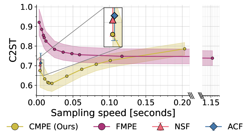
Figure 3: Experiment 1 (Gaussian Mixture Model). Plots show average C2ST and its standard deviation over a test set of size $J=100$, as a function of each method’s sampling speed for 1000 posterior draws. CMPE (ours) outperforms all other methods through both faster and better inference, as indexed by lower (better) C2ST scores. Mind the broken $x$-axis.

5.1 Experiment 1: Gaussian Mixture Model

We illustrate CMPE on a 2-dimensional Gaussian mixture model with two symmetrical components (Geffner et al., 2022; Schmitt et al., 2023a). The symmetrical components are equally weighted and have equal variance,

$$\boldsymbol{\theta}\sim\mathcal{N}(\boldsymbol{\theta}\,|\,\mathbf{0},\mathbf{I}),\;\mathbf{x}\sim\tfrac{1}{2}\,\mathcal{N}(\mathbf{x}\,|\,\boldsymbol{\theta},\tfrac{\mathbf{I}}{2})+\tfrac{1}{2}\,\mathcal{N}(\mathbf{x}\,|\,{-}\boldsymbol{\theta},\tfrac{\mathbf{I}}{2}),$$ (13)

where $\mathcal{N}(\cdot\,|\,\mathbf{\mu},\mathbf{\Sigma})$ is a Gaussian distribution with location $\mathbf{\mu}$ and covariance matrix $\mathbf{\Sigma}$. The resulting posterior distribution is bimodal and point-symmetric around the origin (see Figure 2 top-left). Each simulated data set $\mathbf{x}$ consists of ten exchangeable observations $\{\mathbf{x}_{1},\ldots,\mathbf{x}_{10}\}$, and we train all architectures on $M=1024$ training simulations. We use a DeepSet (Zaheer et al., 2017) to learn 6 summary statistics for each data set jointly with the inference task.

Results

As displayed in Figure 2, both ACF and NSF fail to fit the bimodal posterior with separated modes. FMPE successfully forms disconnected posterior modes, but shows visible overconfidence through overly narrow posteriors. The visual sampling performance of CMPE is superior to all other methods. In this task, we observe that CMPE does not force us to choose between speed or performance relative to the other approximators. Instead, CMPE can outperform all other methods simultaneously with respect to both speed and performance, as evidenced by lower C2ST to the reference posterior across $J=100$ test instances (see Figure 3). If we tolerate slower sampling, CMPE achieves peak performance at $K=10$ inference steps. Most notably, CMPE outperforms 1000-step FMPE by a large margin, even though the latter is approximately 75$\times$ slower.

5.2 Experiment 2: Two Moons

This experiment studies the two moons benchmark (Greenberg et al., 2019; Lueckmann et al., 2021; Wiqvist et al., 2021; Radev et al., 2023a). The model is characterized by a bimodal posterior with two separated crescent moons for the observed point $\mathbf{x}_{\text{obs}}=(0,0)^{\top}$ which a posterior approximator needs to recover. We repeat the experiment for different training budgets $M\in\{512,1024,2048,4096,8192\}$ to assess the performance of each method under varying data availability. While $M=512$ is a very small budget for the two moons benchmark, $M=8192$ is generally considered sufficient for this experiment.

Results

Trained on a simulation budget of $M=1024$ examples, CMPE consistently explores both crescent moons and successfully captures the local patterns of the posterior (see Figure 2, middle row). Both the affine coupling flow and the neural spline flow fail to fully separate the modes. Most notably, if we aim to achieve fast sampling speed with FMPE by reducing the number of sampling steps during inference, FMPE shows visible overconfidence with 30 sampling steps and markedly deficient approximate posteriors with 10 sampling steps. In stark contrast, CMPE excels in the few-step regime. Figure 4 illustrates that all architectures benefit from a larger training budget. CMPE with 10 steps emerges as the superior architecture in the low- and medium- data regime up to $M=4096$ training instances. Many-step FMPE outperforms the other approximators for the largest training budget of $M=8192$ instances. Keep in mind, however, that many-step FMPE is approximately 30–70$\times$ slower than ACF, NSF, and CMPE in this task.

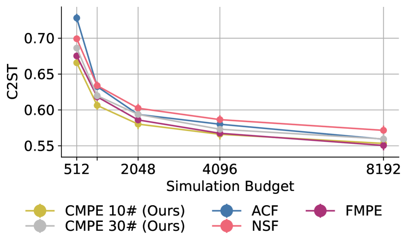
Figure 4: Experiment 2 (Two Moons). CMPE (ours) with 10 sampling steps shows superior performance up to a training budget of 4096 instances. Plots show average C2ST and its standard error over a test set of size $J=100$.

5.3 Experiment 3: Inverse Kinematics

Proposed as a benchmarking task for inverse problems by Kruse et al. (2021), the inverse kinematics model aims to reconstruct the configuration $(\theta_{1},\theta_{2},\theta_{3},\theta_{4})=\boldsymbol{\theta}\in\mathbb{R}^{4}$ of a multi-jointed 2D arm for a given end position $\mathbf{x}\in\mathbb{R}^{2}$ (see Figure 2, bottom left). The forward process $g:\boldsymbol{\theta}\mapsto\mathbf{x}$ takes as inputs the initial height $\theta_{1}$ of the arm’s base, as well as the angles $\theta_{2},\theta_{3},\theta_{4}$ at its three joints. The inverse problem asks for the posterior distribution $p(\boldsymbol{\theta}\,|\,\mathbf{x})$, which represents all arm configurations $\boldsymbol{\theta}$ that end at the observed 2D position $\mathbf{x}$ of the arm’s end effector. The parameters follow a Gaussian prior $\boldsymbol{\theta}\sim\mathcal{N}(\mathbf{0},\boldsymbol{\sigma}^{2}\mathbf{I})$ with $\boldsymbol{\sigma}^{2}=(\frac{1}{16},\frac{1}{4},\frac{1}{4},\frac{1}{4})$. While the parameter space in this task is 4-dimensional, we can readily plug any parameter estimate $\hat{\boldsymbol{\theta}}$ into the forward simulator $g$ to get the corresponding end effector position $g(\hat{\boldsymbol{\theta}})=\hat{\mathbf{x}}\in\mathbb{R}^{2}$, which is easy to visualize and interpret.

Table 2: Experiment 4: RMSE and MMD between the ground-truth image vs. 100 draws from the approximators trained on 2 000 and 60 000 training images, aggregated over 100 test images. For MMD, we draw one denoised sample per test image and calculate the MMD between the denoised samples and the original images. Time per draw.

Models		RMSE $\downarrow$		MMD ($\pm$ SD) [$\times\,10^{-3}$] $\downarrow$		Time $\downarrow$
		2 000	60 000	2 000	60 000
naïve	FMPE	0.836	0.597	$171.53$ $\pm 1.61$	$95.26\pm 1.21$	15.4ms
	CMPE (ours)	0.388	0.293	$\mathbf{102.09}\pm 3.24$	$\mathbf{57.90}\pm 1.59$	0.3ms
U-Net	FMPE	0.278	0.217	$\mathbf{17.38}\pm 0.10$	$\mathbf{14.50}\pm 0.05$	565.8ms
	CMPE (ours)	0.311	0.238	$18.49\pm 0.12$	$16.08\pm 0.05$	0.5ms

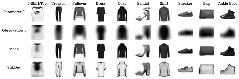
Figure 5: Experiment 4. CMPE denoising results from each class of Fashion MNIST obtained using a U-Net architecture and two-step sampling. A training set of 60 000 images was used. First row: Original image acting as the “parameters” of the noisy camera simulator. Second row: Blurred image, acting as the output of the camera simulator. Third and fourth row: Means and standard deviations of the posteriors estimated from the corresponding blurry “observations”. Note: For standard deviations, darker regions indicate larger variability in the outputs. Adapted from Radev et al. (2023a).

Results

On the challenging small training budget of $M=1024$ training examples, CMPE with $K=30$ sampling steps clearly outperforms all other methods while maintaining fast inference (see Figure 2).

5.4 Experiment 4: Bayesian Denoising

This experiment demonstrates the feasibility of CMPE for a high-dimensional inverse problem, namely, Bayesian denoising on the Fashion MNIST data set. The unknown parameter $\boldsymbol{\theta}\in\mathbb{R}^{784}$ is the flattened original image, and the observation $\mathbf{x}\in\mathbb{R}^{784}$ is a blurred and flattened version of the crisp image from a simulated noisy camera (Ramesh et al., 2022; Pacchiardi & Dutta, 2022; Radev et al., 2023a).

We compare CMPE and FMPE in a standard and a small data regime. As both methods allow for free-form architectures, we can assess the effect of the architectural choices on the results. Therefore, we evaluate both methods using a suboptimal naïve architecture and the established U-Net (Ronneberger et al., 2015) architecture.

Neural architectures

The naïve architecture consists of a convolutional neural network (CNN; LeCun et al., 2015) to convert the observation into a vector of latent summary statistics. We concatenate input vector, summary statistics, and a time embedding and feed them into a multi-layer perceptron (MLP) with four hidden layers consisting of 2048 units each. This corresponds to a situation where the structure of the observation (i.e., image data) is known, but the structure of the parameters is unknown or does not inform a bespoke network architecture.

In this example, however, we can leverage the prior knowledge that our parameters are images. Specifically, we can incorporate inductive biases into our network architecture by choosing a U-Net architecture which is optimized for image processing (i.e., an adapted version of Nain, 2022). Again, a CNN learns a summary vector of the noisy observation, which is then concatenated with a time embedding into the condition vector for the neural density estimator.

Results

We provide the aggregated RMSE, MMD, and the time per sample for both methods and both architectures (Table 2). FMPE is not able to generate good samples for the naïve architecture, whereas CMPE produces acceptable samples even in this suboptimal setup. This reduced susceptibility to suboptimal architectural choices might become a valuable feature in high-dimensional problems where the structure of the parameters cannot be exploited. The U-Net architecture enables good sample quality for both methods, highlighting the advantages of free-form architectures. The MMD values align well with our subjective visual assessment of the sample quality, therefore we deem it an informative metric to compare the results. Please refer to the samples in Section B.4 for visual inspection and comparison. The U-Net architecture paired with a large training set provides detailed and variable samples of similar quality for CMPE and FMPE. In all cases, CMPE exhibits significantly lower inference time as only two network passes are required for sampling, while achieving better or competitive quality.

Table 3: Experiment 5. RMSE, ECE, and sampling time are computed for 2000 posterior samples, aggregated over 400 unseen test instances. Max ECE denotes the worst-case marginal calibration error across all 7 model parameters.

Model	RMSE $\downarrow$	Max ECE $\downarrow$	Time $\downarrow$
ACF	0.589	0.021	1.07s
NSF	0.590	0.027	1.95s
FMPE 30#	0.582	0.222	17.13s
FMPE 1000#	0.583	0.057	500.90s
CMPE 2# (Ours)	0.616	0.064	2.16s
CMPE 30# (Ours)	0.577	0.018	18.33s

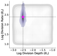
(a) CMPE (ours) 2 steps

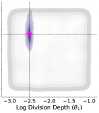
(b) CMPE (ours) 30 steps

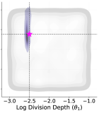
(c) FMPE 30 steps

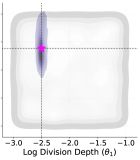
(d) FMPE 1000 steps

Figure 6: Experiment 5. Posterior draws for two parameters of the tumor growth model, based on one fixed data set $\mathbf{x}$. Cross-hair and pink star indicate the ground-truth parameter that we aim to recover. The gray region depicts the prior distribution. CMPE (ours) shows no visible bias even for two-step inference, but a clearly improved sharpness when we increase the number of sampling steps to 30. In contrast, FMPE with 30 sampling steps (i.e., comparable inference speed to CMPE) suffers from notable bias. The posterior of FMPE with 1000 inference steps visibly improves, enveloping the ground-truth, but remains slightly worse than CMPE with 30 sampling steps.

5.5 Experiment 5: Tumor Spheroid Growth

We conclude our empirical evaluation with a complex multi-scale model of 2D tumor spheroid growth (Jagiella et al., 2017). The model has $7$ unknown parameters which are to be recovered from high-dimensional summary statistics (original simulation settings taken from pyABC, 2017). Crucially, running simulations from this model on standard hardware is rather expensive ($\approx 1$ minute for a single run on a consumer-grade computer), so there is a desire for methods that can provide reasonable estimates for a limited offline training budget. Here, we compare the performance of the four contender methods in this paper, namely, ACF, NSF, FMPE, and CMPE, on a fixed training set of $M=19\,600$ simulations with $J=400$ simulations as a test set to compute performance metrics.

Neural architectures

To compress the high-dimensional summary statistics into fixed vectors, we employ a custom hybrid LSTM-Transformer architecture which can deal with multiple time series inputs of different lengths. All contender methods share the same summary network architecture. In addition, CMPE and FMPE use the same free-form base inference model, and ACF and NSF rely on the same architecture for the internal coupling layers. Section B.5 provides more details on the neural network architectures and training hyperparameters.

Results

CMPE outperforms the alternative neural methods through better accuracy and calibration, as indexed by a lower RMSE and ECE on 400 unseen test instances (see Table 3). The speed of the simpler ACF is unmatched by the other contenders. In direct comparison to its free-form contender FMPE, CMPE simultaneously exhibits (i) a slightly higher accuracy; (ii) a drastically improved calibration; and (iii) much faster sampling. For this model, FMPE did not achieve satisfactory calibration performance even with up to $K=100$ inference steps, so Table 3 reports the best FMPE results for $K=1000$ inference steps.

6 Conclusion

In this paper, we presented consistency model posterior estimation (CMPE), a state-of-the-art approach to perform accurate simulation-based Bayesian inference on large-scale models while achieving fast inference speed. CMPE enhances the capabilities of neural posterior estimation by combining the free-form neural architecture property of diffusion models and flow matching with high-performing few-step sampling schemes.

To assess the effectiveness of CMPE, we applied it to a set of 3 low-dimensional benchmark tasks that allow intuitive visual inspection, as well as a relatively high-dimensional Bayesian denoising experiment and a scientifically relevant tumor growth model. Across all experiments, CMPE consistently outperforms all other established methods based on a holistic assessment of posterior accuracy, calibration, and inference speed.

Future work might aim to further reduce the number of sampling steps towards one-step inference, for instance, via extensive automated hyperparameter optimization or tailored training schemes for the simulation-based training regime of CMPE. Overall, our results underscore the potential of CMPE as a novel simulation-based inference tool, rendering it a new contender for applied simulation-based inference workflows in science and engineering.

Acknowledgments

We thank Lasse Elsemüller for insightful feedback and thought-provoking ideas. MS acknowledges the funding of the Cyber Valley Research Fund (grant number: CyVy-RF-2021-16) and the Deutsche Forschungsgemeinschaft (DFG, German Research Foundation) under Germany’s Excellence Strategy EXC-2075 - 390740016 (the Stuttgart Cluster of Excellence SimTech). MS additionally thanks the Google Cloud Research Credits program and the European Laboratory for Learning and Intelligent Systems (ELLIS) PhD program for support. VP acknowledges funding by the German Academic Exchange Service (DAAD) and the German Federal Ministry of Education and Research (BMBF) through the funding programme “Konrad Zuse Schools of Excellence in Artificial Intelligence” (ELIZA) and support by the state of Baden-Württemberg through bwHPC. VP acknowledges support by the Bundesministerium fuer Wirtschaft und Klimaschutz (BMWK, German Federal Ministry for Economic Affairs and Climate Action) as part of the German government’s 7th energy research program “Innovations for the energy transition” under the 03ETE039I HiBRAIN project (Holistic method of a combined data- and model-based Electrode design supported by artificial intelligence).

Appendix A Consistency training details

Table 4 details all functions and parameters required for training. Except for the choice of parameters $s_{0}$, $s_{1}$, $\varepsilon$, $T_{\text{max}}$ and $\sigma_{\text{data}}$ we exactly follow the design choices proposed by Song & Dhariwal (2023), which improved our results compared to the choices in Song et al. (2023). Song & Dhariwal (2023) showed that that the Exponential Moving Average of the teacher’s parameter $\boldsymbol{\phi}^{-}$ should not be used in Consistency Training, therefore we omitted it in this paper.

Table 4: Design choices: Table and values adapted to our notation from Song & Dhariwal (2023, Table 1).

Metric in consistency loss	$d(\mathbf{x},\mathbf{y})=\sqrt{\lVert\mathbf{x}-\mathbf{y}\rVert_{2}^{2}+c^{2}}-c$
Discretization curriculum	$N(k)=\min(s_{0}2^{\lfloor k/K^{\prime}\rfloor},s_{1})+1$ where $K^{\prime}=\lfloor K/(\log_{2}\lfloor s_{1}/s_{0}\rfloor+1)\rfloor$
Noise schedule	$t_{i}$, where $i\sim p(i)$ and $p(i)\sim\text{erf}\left(\frac{\log(t_{i+1})-P_{\text{mean}}}{\sqrt{2}P_{\text{std}}}\right)-\text{erf}\left(\frac{\log(t_{i})-P_{\text{mean}}}{\sqrt{2}P_{\text{std}}}\right)$
Weighting function	$\lambda(t_{i})=1/(t_{i+1}-t_{i})$
Skip connections	$c_{\text{skip}}(t)=\sigma^{2}_{\text{data}}/((t-\varepsilon)^{2}+\sigma_{\text{data}}^{2})$, $c_{\text{out}}(t)=\sigma_{\text{data}}(t-\varepsilon)/\sqrt{\sigma_{\text{data}}^{2}+t^{2}}$
Parameters	$s_{0}=10,s_{1}=50$ except where indicated otherwise
	$c=0.00054\sqrt{d}$, where $d$ is the dimensionality of $\theta$
	$P_{\text{mean}}=-1.1,P_{\text{std}}=2.0$
	$k\in{0,\dots,K-1}$, where K is the total training iterations
	$t_{i}=\left(\varepsilon^{1/\rho}+\frac{i+1}{N(k)-1}\left(T_{\text{max}}^{1/\rho}-\varepsilon^{1/\rho}\right)\right)^{\rho}$, $\rho=7$, $\varepsilon=0.001$, $T_{\text{max}}=200$

Appendix B Additional details and results

B.1 Experiment 1

Neural network details

All architectures use a summary network to learn fixed-length representations of the $i.i.d.$ data $\mathbf{x}=\{\mathbf{x}_{1},\ldots,\mathbf{x}_{10}\}$. We implement this via a DeepSet (Zaheer et al., 2017) with 6-dimensional output. Both ACF and NSF use 4 coupling layers and train for 200 epochs with a batch size 32. CMPE relies on an MLP with 2 hidden layers of 256 units each, L2 regularization with weight $10^{-4}$, 10% dropout and an initial learning rate of $10^{-4}$. The consistency model is instantiated with the hyperparameters $s_{0}=10,s_{1}=1280,T_{\text{max}}=1$. Training is based on 2000 epochs with batch size 64. FMPE and CMPE use an identical MLP, and the only difference is the initial learning rate of $10^{-5}$ for FMPE to alleviate instable training dynamics.

B.2 Experiment 2

Neural network details

CMPE uses an MLP with 2 layers of 256 units each, L2 regularization with weight $10^{-5}$, 5% dropout, and an initial learning rate of $5\cdot 10^{-4}$. The consistency model uses $s_{0}=10,s_{1}=50,T_{\text{max}}=10$, and it is trained with a batch size of 64 for 5000 epochs. Both ACF and NSF use 6 coupling layers of 128 units each, kernel regularization with weight $\gamma=10^{-4}$, and train for 200 epochs with a batch size 32. FMPE uses the same settings and training configuration as CMPE.

B.3 Experiment 3

Neural network details

CMPE relies on an MLP with 2 layers of 256 units each, L2 regularization with weight $10^{-5}$, 5% dropout, and an initial learning rate of $5\times 10^{-4}$. The consistency model uses $s_{0}=10,s_{1}=50$, and trains for 2000 epochs with a batch size of 32. FMPE uses the same MLP and training configuration as CMPE. Both ACF and NSF use 6 coupling layers of 128 units each, kernel regularization with weight $\gamma=10^{-4}$, and train for 200 epochs with a batch size 32.

B.4 Experiment 4

We compare samples from a $2\times 2\times 2$ design: Two methods, CMPE and FMPE, are trained on two network architectures, a naïve architecture and a U-Net architecture, using 2 000 and 60 000 training images. Except for the batch size, which is 32 for 2 000 training images and 256 for 60 000 training images, all hyperparameters are held constant between all runs. We use an AdamW optimizer with a learning rate of $5\cdot 10^{-4}$ and cosine decay for 20 000 iterations, rounded up to the next full epoch. As both methods use the same network sizes, this results in an approximately equal training time between methods (approximately 1-2 hours on a Tesla V100 GPU), with a significantly lower training time for the naïve architecture.

Neural network details

For CMPE, we use $s_{0}=10,s_{1}=50$, $\sigma_{\text{data}}^{2}=0.25$ and two-step sampling. For FMPE, we follow Dax et al. (2023b) and use 248 network passes. Note that this is directly correlated with inference time: Choosing a lower value will make FMPE sampling faster, a larger value will slow down FMPE sampling.

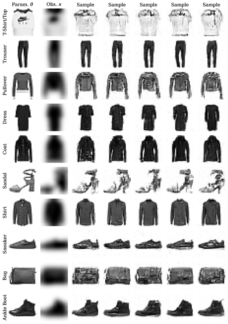
Figure 7: CMPE - U-Net architecture - 2 000 training images. CMPE denoising results from each class of Fashion MNIST obtained using a U-Net architecture and two-step sampling. A small training set of 2 000 images was used.

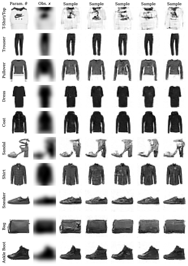
Figure 8: CMPE - U-Net architecture - 60 000 training images. CMPE denoising results from each class of Fashion MNIST obtained using a U-Net architecture and two-step sampling. A large training set of 60 000 images was used.

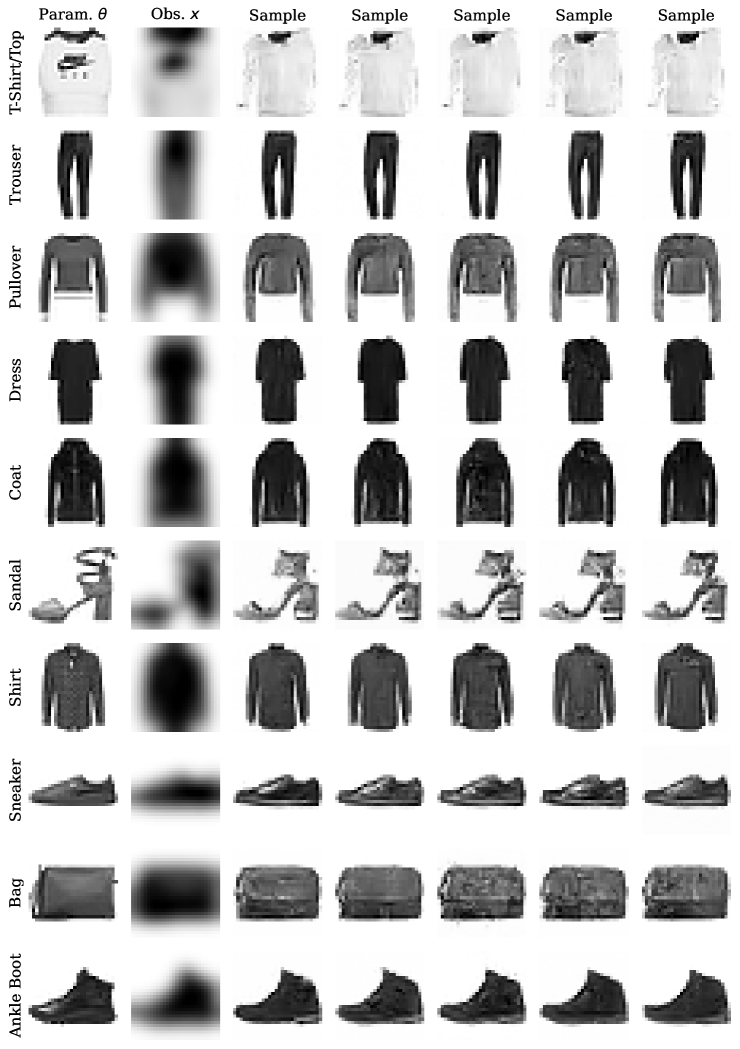
Figure 9: FMPE - U-Net architecture - 2 000 training images. FMPE denoising results from each class of Fashion MNIST obtained using a U-Net architecture. A small training set of 2 000 images was used.

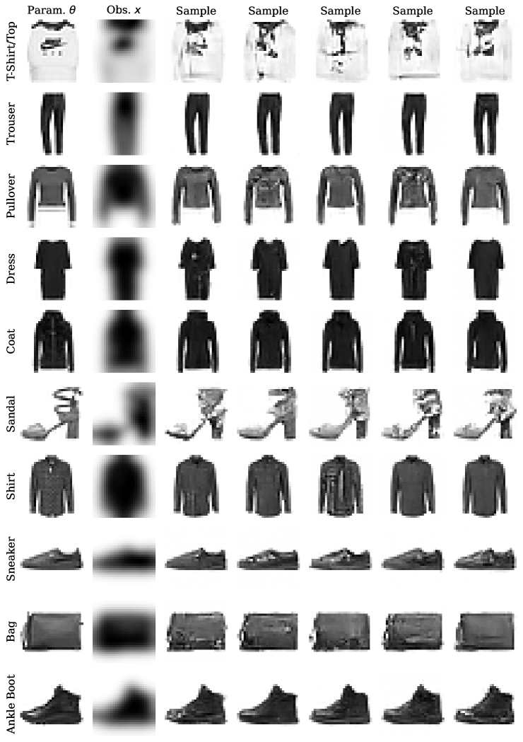
Figure 10: FMPE - U-Net architecture - 60 000 training images. FMPE denoising results from each class of Fashion MNIST obtained using a U-Net architecture. A large training set of 60 000 images was used.

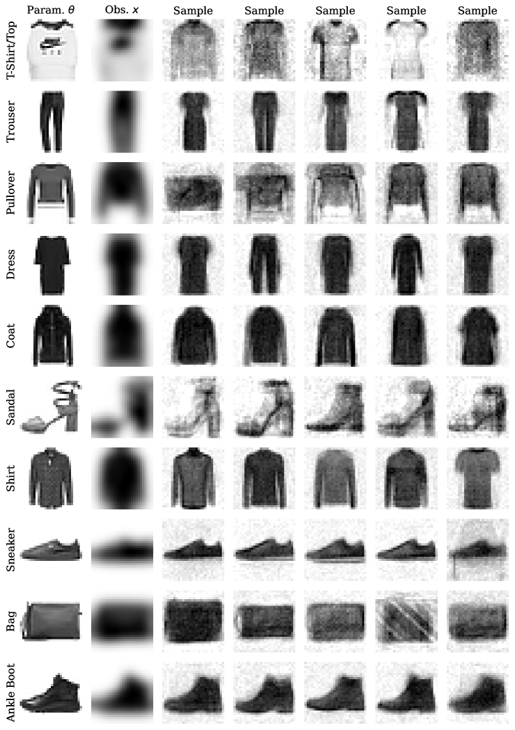
Figure 11: CMPE - Naïve architecture - 2 000 training images. CMPE denoising results from each class of Fashion MNIST obtained using the naïve architecture described above and two-step sampling. A small training set of 2 000 images was used.

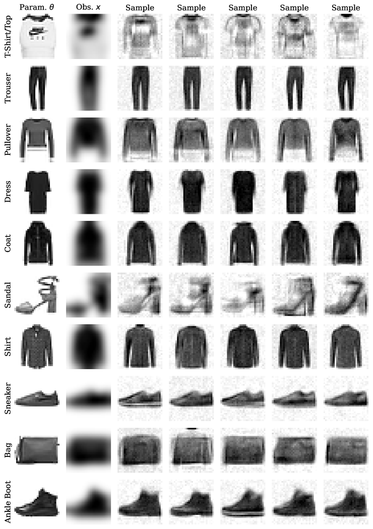
Figure 12: CMPE - Naïve architecture - 60 000 training images. CMPE denoising results from each class of Fashion MNIST obtained using the naïve architecture described above and two-step sampling. A large training set of 60 000 images was used.

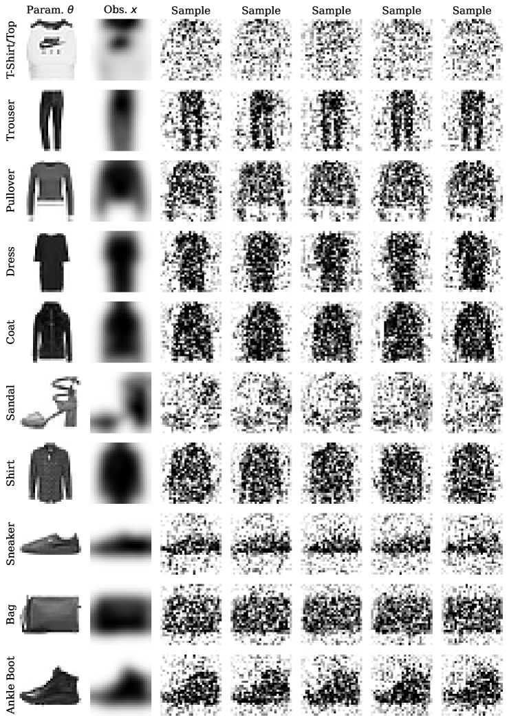
Figure 13: FMPE - Naïve architecture - 2 000 training images. FMPE denoising results from each class of Fashion MNIST obtained using the naïve architecture described above. A small training set of 2 000 images was used.

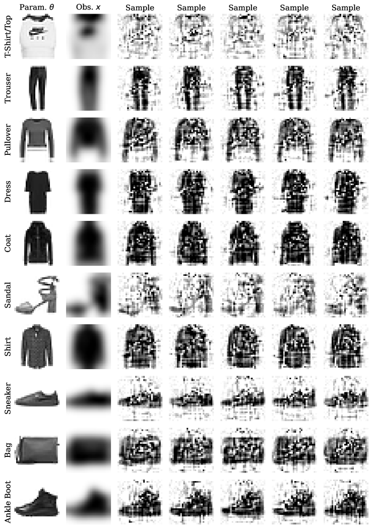
Figure 14: FMPE - Naïve architecture - 60 000 training images. CMPE denoising results from each class of Fashion MNIST obtained using the naïve architecture described above. A large training set of 60 000 images was used.

B.5 Experiment 5

Neural network details

Both CMPE and FMPE use an MLP with 4 hidden layers of 512 units each and 20% dropout. CMPE and FMPE train for 1000 epochs with a batch size of 64. The consistency model uses $s_{0}=10,s_{1}=50,T_{\text{max}}=50$. ACF and NSF employ a coupling architecture with learnable permutations, 6 coupling layers of 128 units each, 20% dropout, and 300 epochs of training with a batch size of 64.

The input data consists of multiple time series of different lengths. As proposed by Schmitt et al. (2023b) for SBI with heterogeneous data sources, we employ a late fusion scheme where the input modalities are first processed by individual embedding networks, and then fused. First, the data on tumor size growth curves enters an LSTM which produces a 16-dimensional representation of this modality. Second, the information about radial features is processed by a temporal fusion transformer with 4 attention heads, 64-dimensional keys, 128 units per fully-connected layer, and $10^{-4}$ L2 regularization on both weights and biases. These latent representations are then concatenated and further fed through a fully-connected two-layer perceptron of 256 units each, $10^{-4}$ L2 regularization on weights and biases, and 32 output dimensions.

References

- Ardizzone et al. (2019) Ardizzone, L., Kruse, J., Wirkert, S., Rahner, D., Pellegrini, E. W., Klessen, R. S., Maier-Hein, L., Rother, C., and Köthe, U. Analyzing inverse problems with invertible neural networks. In Intl. Conf. on Learning Representations, 2019.
- Avecilla et al. (2022) Avecilla, G., Chuong, J. N., Li, F., Sherlock, G., Gresham, D., and Ram, Y. Neural networks enable efficient and accurate simulation-based inference of evolutionary parameters from adaptation dynamics. PLoS Biology, 20(5):e3001633, 2022.
- Batzolis et al. (2021) Batzolis, G., Stanczuk, J., Schönlieb, C.-B., and Etmann, C. Conditional image generation with score-based diffusion models, 2021.
- Bieringer et al. (2021) Bieringer, S., Butter, A., Heimel, T., Höche, S., Köthe, U., Plehn, T., and Radev, S. T. Measuring qcd splittings with invertible networks. SciPost Physics, 10(6):126, 2021.
- Boelts et al. (2023) Boelts, J., Harth, P., Gao, R., Udvary, D., Yáñez, F., Baum, D., Hege, H.-C., Oberlaender, M., and Macke, J. H. Simulation-based inference for efficient identification of generative models in computational connectomics. February 2023. doi: 10.1101/2023.01.31.526269. URL https://doi.org/10.1101/2023.01.31.526269.
- Briol et al. (2019) Briol, F.-X., Barp, A., Duncan, A. B., and Girolami, M. Statistical inference for generative models with maximum mean discrepancy, 2019.
- Bürkner et al. (2023) Bürkner, P.-C., Scholz, M., and Radev, S. T. Some models are useful, but how do we know which ones? towards a unified bayesian model taxonomy. Statistics Surveys, 17(none), 2023. ISSN 1935-7516. doi: 10.1214/23-ss145. URL http://dx.doi.org/10.1214/23-SS145.
- Butter et al. (2022) Butter, A., Plehn, T., Schumann, S., Badger, S., Caron, S., Cranmer, K., Di Bello, F. A., Dreyer, E., Forte, S., Ganguly, S., et al. Machine learning and lhc event generation. arXiv preprint arXiv:2203.07460, 2022.
- Cranmer et al. (2020) Cranmer, K., Brehmer, J., and Louppe, G. The frontier of simulation-based inference. Proceedings of the National Academy of Sciences, 2020.
- Dax et al. (2023a) Dax, M., Green, S. R., Gair, J., Pürrer, M., Wildberger, J., Macke, J. H., Buonanno, A., and Schölkopf, B. Neural importance sampling for rapid and reliable gravitational-wave inference. Physical Review Letters, 130(17), April 2023a. ISSN 1079-7114. doi: 10.1103/physrevlett.130.171403. URL http://dx.doi.org/10.1103/PhysRevLett.130.171403.
- Dax et al. (2023b) Dax, M., Wildberger, J., Buchholz, S., Green, S. R., Macke, J. H., and Schölkopf, B. Flow matching for scalable simulation-based inference, 2023b.
- Deistler et al. (2022) Deistler, M., Goncalves, P. J., and Macke, J. H. Truncated proposals for scalable and hassle-free simulation-based inference. arXiv preprint, 2022.
- Dinh et al. (2016) Dinh, L., Sohl-Dickstein, J., and Bengio, S. Density estimation using real nvp. arXiv preprint arXiv:1605.08803, 2016.
- Durkan et al. (2019) Durkan, C., Bekasov, A., Murray, I., and Papamakarios, G. Neural spline flows. Advances in neural information processing systems, 32, 2019.
- Durkan et al. (2020) Durkan, C., Murray, I., and Papamakarios, G. On contrastive learning for likelihood-free inference. In International Conference on Machine Learning. PMLR, 2020.
- Elsemüller et al. (2023a) Elsemüller, L., Olischläger, H., Schmitt, M., Bürkner, P.-C., Köthe, U., and Radev, S. T. Sensitivity-aware amortized Bayesian inference, 2023a. arXiv:2310.11122.
- Elsemüller et al. (2023b) Elsemüller, L., Schnuerch, M., Bürkner, P.-C., and Radev, S. T. A deep learning method for comparing bayesian hierarchical models, 2023b.
- Engel et al. (2020) Engel, J., Resnick, C., Roberts, A., Dieleman, S., Norouzi, M., Eck, D., and Simonyan, K. Ddsp: Differentiable digital signal processing. In International Conference on Learning Representations, 2020.
- Geffner et al. (2022) Geffner, T., Papamakarios, G., and Mnih, A. Compositional score modeling for simulation-based inference, 2022.
- Ghaderi-Kangavari et al. (2023) Ghaderi-Kangavari, A., Rad, J. A., and Nunez, M. D. A general integrative neurocognitive modeling framework to jointly describe EEG and decision-making on single trials. Computational Brain and Behavior, 2023. doi: 10.1007/s42113-023-00167-4.
- Gonçalves et al. (2020) Gonçalves, P. J., Lueckmann, J.-M., Deistler, M., et al. Training deep neural density estimators to identify mechanistic models of neural dynamics. Elife, 2020.
- Goodfellow et al. (2014) Goodfellow, I., Pouget-Abadie, J., Mirza, M., Xu, B., Warde-Farley, D., Ozair, S., Courville, A., and Bengio, Y. Generative adversarial nets. In Ghahramani, Z., Welling, M., Cortes, C., Lawrence, N., and Weinberger, K. (eds.), Advances in Neural Information Processing Systems, volume 27. Curran Associates, Inc., 2014.
- Greenberg et al. (2019) Greenberg, D., Nonnenmacher, M., and Macke, J. Automatic posterior transformation for likelihood-free inference. In International Conference on Machine Learning, 2019.
- Gretton et al. (2012) Gretton, A., Borgwardt, K., Rasch, M., Schölkopf, B., and Smola, A. A Kernel Two-Sample Test. The Journal of Machine Learning Research, 13:723–773, 2012.
- Heringhaus et al. (2022) Heringhaus, M. E., Zhang, Y., Zimmermann, A., and Mikelsons, L. Towards reliable parameter extraction in mems final module testing using bayesian inference. Sensors, 22(14):5408, July 2022. ISSN 1424-8220. doi: 10.3390/s22145408. URL http://dx.doi.org/10.3390/s22145408.
- Ho et al. (2020) Ho, J., Jain, A., and Abbeel, P. Denoising diffusion probabilistic models. In Advances in Neural Information Processing Systems, volume 33, pp. 6840–6851, 2020.
- Jadhao et al. (2012) Jadhao, V., Solis, F. J., and de la Cruz, M. O. Simulation of Charged Systems in Heterogeneous Dielectric Media via a True Energy Functional. Physical Review Letters, 109(22), 2012. doi: 10.1103/physrevlett.109.223905.
- Jagiella et al. (2017) Jagiella, N., Rickert, D., Theis, F. J., and Hasenauer, J. Parallelization and high-performance computing enables automated statistical inference of multi-scale models. Cell systems, 4(2):194–206, 2017.
- Kadupitiya et al. (2020) Kadupitiya, J., Sun, F., Fox, G., and Jadhao, V. Machine learning surrogates for molecular dynamics simulations of soft materials. Journal of Computational Science, 42:101107, 2020. doi: 10.1016/j.jocs.2020.101107.
- Karras et al. (2022) Karras, T., Aittala, M., Aila, T., and Laine, S. Elucidating the design space of diffusion-based generative models. Advances in Neural Information Processing Systems, 35:26565–26577, 2022.
- Köthe (2023) Köthe, U. A review of change of variable formulas for generative modeling. arXiv preprint arXiv:2308.02652, 2023.
- Kruse et al. (2021) Kruse, J., Ardizzone, L., Rother, C., and Köthe, U. Benchmarking invertible architectures on inverse problems. 2021. Workshop on Invertible Neural Networks and Normalizing Flows (ICML 2019).
- Lavin et al. (2021) Lavin, A., Zenil, H., Paige, B., et al. Simulation intelligence: Towards a new generation of scientific methods. arXiv preprint, 2021.
- LeCun et al. (2015) LeCun, Y., Bengio, Y., and Hinton, G. Deep learning. Nature, 521(7553):436–444, 2015. ISSN 1476-4687. doi: 10.1038/nature14539. URL http://dx.doi.org/10.1038/nature14539.
- Lipman et al. (2023) Lipman, Y., Chen, R. T. Q., Ben-Hamu, H., Nickel, M., and Le, M. Flow matching for generative modeling. In The 11th International Conference on Learning Representations, 2023. URL https://openreview.net/forum?id=PqvMRDCJT9t.
- Liu et al. (2022) Liu, X., Gong, C., and Liu, Q. Flow straight and fast: Learning to generate and transfer data with rectified flow, 2022.
- Lueckmann et al. (2017) Lueckmann, J.-M., Gonçalves, P. J., Bassetto, G., Öcal, K., Nonnenmacher, M., and Macke, J. H. Flexible statistical inference for mechanistic models of neural dynamics. In 31st NeurIPS Conference Proceedings, 2017.
- Lueckmann et al. (2021) Lueckmann, J.-M., Boelts, J., Greenberg, D. S., Gonçalves, P. J., and Macke, J. H. Benchmarking simulation-based inference. arXiv preprint, 2021.
- Nain (2022) Nain, A. K. Keras documentation: Denoising diffusion probabilistic model. https://keras.io/examples/generative/ddpm/, 2022. Accessed: 2023-11-27.
- Pacchiardi & Dutta (2022) Pacchiardi, L. and Dutta, R. Score matched neural exponential families for likelihood-free inference. J. Mach. Learn. Res., 23:38–1, 2022.
- Papamakarios & Murray (2016) Papamakarios, G. and Murray, I. Fast -free inference of simulation models with bayesian conditional density estimation. Advances in neural information processing systems, 29, 2016.
-
pyABC (2017)
pyABC.
pyABC documentation, multi-scale model: Tumor spheroid growth.
https://pyabc.readthedocs.io/en/latest/examples/
multiscale_agent_based.html, 2017. Accessed: 2023-12-07. - Radev et al. (2020) Radev, S. T., Mertens, U. K., Voss, A., Ardizzone, L., and Köthe, U. Bayesflow: Learning complex stochastic models with invertible neural networks. IEEE transactions on neural networks and learning systems, 2020.
- Radev et al. (2021a) Radev, S. T., D’Alessandro, M., Mertens, U. K., Voss, A., Köthe, U., and Bürkner, P.-C. Amortized bayesian model comparison with evidential deep learning. IEEE Transactions on Neural Networks and Learning Systems, 2021a.
- Radev et al. (2021b) Radev, S. T., Graw, F., Chen, S., Mutters, N. T., Eichel, V. M., Bärnighausen, T., and Köthe, U. Outbreakflow: Model-based bayesian inference of disease outbreak dynamics with invertible neural networks and its application to the covid-19 pandemics in germany. PLoS computational biology, 2021b.
- Radev et al. (2023a) Radev, S. T., Schmitt, M., Pratz, V., Picchini, U., Köthe, U., and Bürkner, P.-C. JANA: Jointly Amortized Neural Approximation of Complex Bayesian Models. In Evans, R. J. and Shpitser, I. (eds.), Proceedings of the 39th Conference on Uncertainty in Artificial Intelligence, volume 216 of Proceedings of Machine Learning Research, pp. 1695–1706. PMLR, 2023a.
- Radev et al. (2023b) Radev, S. T., Schmitt, M., Schumacher, L., Elsemüller, L., Pratz, V., Schälte, Y., Köthe, U., and Bürkner, P.-C. Bayesflow: Amortized bayesian workflows with neural networks. Journal of Open Source Software, 8(89):5702, 2023b. doi: 10.21105/joss.05702. URL https://doi.org/10.21105/joss.05702.
- Ramesh et al. (2022) Ramesh, P., Lueckmann, J.-M., Boelts, J., Tejero-Cantero, Á., Greenberg, D. S., Gonçalves, P. J., and Macke, J. H. Gatsbi: Generative adversarial training for simulation-based inference. arXiv preprint arXiv:2203.06481, 2022.
- Rombach et al. (2022) Rombach, R., Blattmann, A., Lorenz, D., Esser, P., and Ommer, B. High-resolution image synthesis with latent diffusion models. In Proceedings of the IEEE/CVF Conference on Computer Vision and Pattern Recognition (CVPR), pp. 10684–10695, 2022.
- Ronneberger et al. (2015) Ronneberger, O., Fischer, P., and Brox, T. U-net: Convolutional networks for biomedical image segmentation. In Navab, N., Hornegger, J., Wells, W. M., and Frangi, A. F. (eds.), Medical Image Computing and Computer-Assisted Intervention – MICCAI 2015, pp. 234–241, Cham, 2015. Springer International Publishing. ISBN 978-3-319-24574-4.
- Schmitt et al. (2023a) Schmitt, M., Habermann, D., Bürkner, P.-C., Koethe, U., and Radev, S. T. Leveraging self-consistency for data-efficient amortized Bayesian inference. In NeurIPS UniReps: the First Workshop on Unifying Representations in Neural Models, 2023a.
- Schmitt et al. (2023b) Schmitt, M., Radev, S. T., and Bürkner, P.-C. Fuse it or lose it: Deep fusion for multimodal simulation-based inference, 2023b. arXiv:2311.10671.
- Sharrock et al. (2022) Sharrock, L., Simons, J., Liu, S., and Beaumont, M. Sequential neural score estimation: Likelihood-free inference with conditional score based diffusion models, 2022.
- Shiono (2021) Shiono, T. Estimation of agent-based models using Bayesian deep learning approach of BayesFlow. Journal of Economic Dynamics and Control, 125:104082, 2021.
- Song & Dhariwal (2023) Song, Y. and Dhariwal, P. Improved Techniques for Training Consistency Models, October 2023.
- Song & Ermon (2019) Song, Y. and Ermon, S. Generative modeling by estimating gradients of the data distribution. In Proceedings of the 33rd International Conference on Neural Information Processing Systems, 2019.
- Song et al. (2021) Song, Y., Sohl-Dickstein, J., Kingma, D. P., Kumar, A., Ermon, S., and Poole, B. Score-based generative modeling through stochastic differential equations. In International Conference on Learning Representations, 2021.
- Song et al. (2023) Song, Y., Dhariwal, P., Chen, M., and Sutskever, I. Consistency models. In International Conference on Machine Learning, 2023.
- Talts et al. (2018) Talts, S., Betancourt, M., Simpson, D., Vehtari, A., and Gelman, A. Validating bayesian inference algorithms with simulation-based calibration. arXiv preprint, 2018.
- von Krause et al. (2022) von Krause, M., Radev, S. T., and Voss, A. Mental speed is high until age 60 as revealed by analysis of over a million participants. Nature Human Behaviour, 6(5):700–708, May 2022. doi: 10.1038/s41562-021-01282-7.
- Vondrick et al. (2016) Vondrick, C., Pirsiavash, H., and Torralba, A. Generating videos with scene dynamics. Advances in Neural Information Processing Systems, 29, 2016.
- Wiqvist et al. (2021) Wiqvist, S., Frellsen, J., and Picchini, U. Sequential neural posterior and likelihood approximation. arXiv preprint, 2021.
- Zaheer et al. (2017) Zaheer, M., Kottur, S., Ravanbakhsh, S., Poczos, B., Salakhutdinov, R., and Smola, A. Deep sets, 2017.