0.1% Data Makes Segment Anything Slim

Abstract

The formidable model size and demanding computational requirements of Segment Anything Model (SAM) have rendered it cumbersome for deployment on resource-constrained devices. Existing approaches for SAM compression typically involve training a new network from scratch, posing a challenging trade-off between compression costs and model performance. To address this issue, this paper introduces SlimSAM, a novel SAM compression method that achieves superior performance with remarkably low training costs. This is achieved by the efficient reuse of pre-trained SAMs through a unified pruning-distillation framework. To enhance knowledge inheritance from the original SAM, we employ an innovative alternate slimming strategy that partitions the compression process into a progressive procedure. Diverging from prior pruning techniques, we meticulously prune and distill decoupled model structures in an alternating fashion. Furthermore, a novel label-free pruning criterion is also proposed to align the pruning objective with the optimization target, thereby boosting the post-distillation after pruning. SlimSAM yields significant performance improvements while demanding over 10 times less training costs than any other existing methods. Even when compared to the original SAM-H, SlimSAM achieves approaching performance while reducing parameter counts to merely 0.9% (5.7M), MACs to 0.8% (21G), and requiring only 0.1% (10k) of the SAM training data. Code is available at https://github.com/czg1225/SlimSAM.

1 Introduction

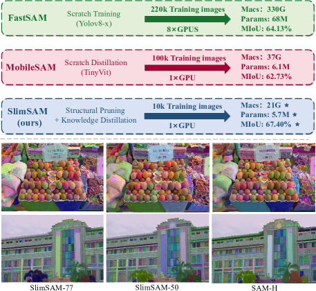
Figure 1: Top: In contrast to scratch training from randomly initialized networks, our approach involves pruning and distilling the original SAM to effectively reusing its pre-trained weights. SlimSAM achieves superior performance with significantly reduced training data. Bottom: Even compared to SAM-H, both SlimSAM-77 (pruning ratio is 77%) and SlimSAM-50 (pruning ratio is 50%) achieve approaching performance.

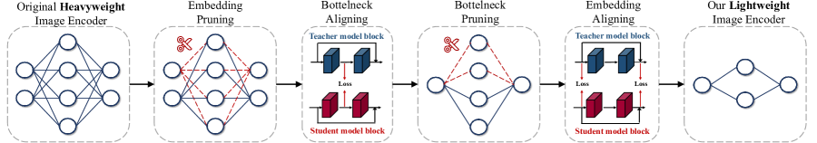
Figure 2: A simple overall diagram of the alternate slimming process employed in our framework.

Segment Anything Model (SAM) [16] has attracted considerable attention from the community since its inception. Owing to its exceptional accuracy in segmentation tasks and next-level generalization capability, SAM has catalyzed notable advancements across a wide spectrum of vision tasks. A plethora of studies [37, 13, 24, 32, 21, 2, 44, 42, 12, 41, 25] have achieved substantial progress by incorporating SAM as a fundamental component. Nevertheless, in spite of its remarkable performance, SAM poses distinct challenges for its practical implementation in industrial applications.

In contrast to Large Language Models (LLMs) [35] designed for cloud-based deployment, SAM demonstrates a pronounced preference for edge deployment. However, SAM’s substantial model size and high computational demands render it inadequate for practical applications on resource-constrained devices. This limitation consequently hinders the advancement and broader application of SAM-based models. Regrettably, only a handful of studies [19, 47, 45] have attempted to address these challenges. Without exception, these endeavors opt to replace the originally heavyweight image encoder with a lightweight and efficient architecture. This invariably entails training a new network from scratch. With regard to scratch training, a challenging trade-off arises between training costs and model performance. On one hand, lower training costs make it difficult to match the performance of the original SAM, which was trained on a dataset of 11 million images. On the other hand, higher training costs, while potentially achieving greater capabilities, require more substantial storage and increased time investment, necessitating more advanced hardware. Existing methods inevitably compromise on performance when training with very limited costs. The fundamental issue lies in the failure to fully leverage the potential of pre-trained SAMs. MobileSAM [45] attempts to employ knowledge distillation to imbue the model with the generalization ability of SAM but still falls short of a complete resolution to this problem. The salient challenge can be summarized as follows: the absence of a general compression method capable of efficiently reusing pre-trained SAMs without the need for extensive re-training.

To tackle the previously mentioned challenge, we introduce SlimSAM, a innovative approach for compressing SAM. SlimSAM combines structural pruning and knowledge distillation [11] technologies to fully reuse the SAM model pre-trained on 11M images, ultimately achieving outstanding compression performance at a minimal training cost. Our primary focus is on compressing the substantial image encoder, as the majority of SAM’s parameter count and computational expenses originate from this component. Structural pruning on channel-wise groups is employed to efficiently reduce the encoder’s size by eliminating redundant parameters and sub-structures from the network. Knowledge distillation is then applied to recover the pruned encoder.

Prior to structural pruning, we employ a dependency detection algorithm to identify all the dependent structures within the model. We introduce a novel label-free importance estimation criterion called disturbed Taylor importance to select the optimal groups for pruning. By generating gradients using model outputs with Gaussian noise, we address the misalignment between pruning target and distillation objective, thereby enhance the distillation-based recovery process.

To minimize disruptions to the original model, SlimSAM adopts an innovative alternate slimming strategy. This approach is distinct from prior methodologies, as it systematically alternates between pruning and distillation of decoupled model structures. The simple diagram of its overall process is depicted in Figure 2. In the initial step, we exclusively prune the embedding dimensions of the encoder while keeping the bottleneck dimensions unchanged. Here, the embedding corresponds to the output of each block within the encoder, whereas the bottleneck represents the intermediate features of each block. Subsequent to this pruning, the distillation recovery aligns both the bottleneck features and the final image embedding. This alignment facilitates faster convergence and enhances the distillation performance. In contrast, following the embedding pruning, we solely prune the bottleneck dimension of ViTs [6], maintaining the embedding dimensions intact. The distillation recovery in this step aligns the final image embedding with the original encoder and aligns the embedding dimensions with the pruned model from the first step. This alternate slimming strategy has demonstrated significant improvements over other general pruning processes.

As shown in Figure 1, our method attains approaching performance while achieving an impressive compression rate in terms of MACs (21G) and Parameters (5.7M), requiring only 0.1% (10k) of the training data compared to the original SAM-H. In comparison to other compacted models, our method yields significant performance improvements while achieving heightened lightweightness and efficiency with substantially less training cost.

In summary, our contribution is a novel SAM compression method called SlimSAM, which efficiently repurposes pre-trained SAMs without the necessity for extensive retraining. This is achieved through the amalgamation of structural pruning and knowledge distillation techniques. By proposing the alternate slimming strategy and introducing the concept of disturbed Taylor importance, we realize greatly enhanced knowledge retention from the original model. SlimSAM achieves approaching performance while reducing the parameter counts to 0.9% (5.7M), MACs to 0.8% (21G), and requiring mere 0.1% (10k) of the training data when compared to the original SAM-H. Extensive experiments demonstrate that our method realize significant superior performance while utilizing over 10 times less training data when compared to other SAM compression methods.

2 Related Works

Model Pruning. Due to the inherent parameter redundancy in deep neural networks [8], model pruning [10, 9, 20, 3, 18, 23, 40] has proved to be an effective approach for accelerating and compressing models. Pruning techniques can be generally classified into two main categories: structural pruning [20, 18, 43, 7, 4, 43] and unstructured pruning [5, 17, 29, 31]. Structural pruning is focused on eliminating parameter groups based on predefined criteria, while unstructured pruning involves the removal of individual weights, typically requiring hardware support. In this work, we showcase the remarkable efficacy of structural pruning on SAM compression.

Knowledge Distillation. Knowledge Distillation (KD) [11] aims to transfer knowledge from a larger, powerful teacher model to a lighter, efficient student model. This process typically involves soft target functions and a temperature parameter to facilitate the learning. KD [34, 33, 46, 1, 39, 22, 36, 26, 28] has gained substantial prominence as an effective technique for model compression across various research domains. In our method, we innovatively employ KD for the efficient recovery of pruned models.

SAM Compression. The formidable model size and computational complexity of SAM pose challenges for edge deployment, yet there is a dearth of research on compressing SAM for practical use. Notably, FastSAM [47] replaces SAM’s extensive ViT-based architecture with the efficient CNN-based YOLOv8-seg [14] model, while MobileSAM [45] adopts the lightweight Tinyvit [38] to replace the image encoder and employs knowledge distillation from the original encoder. However, these approaches inevitably suffer from scratch training, resulting in unsatisfactory performance at a modest training cost. In contrast to existing methods, our SlimSAM achieves superior compression performance while significantly incurring lower training costs by efficiently leveraging the pre-trained SAM.

3 Methods

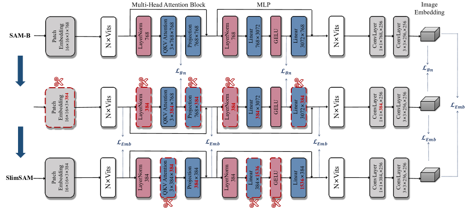
Figure 3: The provided figure depicts our alternate slimming framework with a 50% pruning ratio on SAM-B. We utilize structural pruning at the channel-wise group level to compress SAM’s image encoder, coupled with knowledge distillation from intermediate layers to restore the pruned encoder. The red numbers highlight the pruned dimensions at each pruning step. Initially, we prune dimensions associated with the embeddings and align the bottleneck dimensions. Subsequently, dimensions related to the bottleneck undergo pruning while embedding dimensions are being aligned.

SlimSAM is an innovative framework designed to compress SAM’s heavyweight image encoder through the incorporation of structural pruning and knowledge distillation [11]. We employ a dependency detection algorithm [7] to automatically identify interconnected structures within the model. Once these interrelated structures are identified, weights within the same group are pruned simultaneously to ensure consistency in intermediate representations. Structural pruning is applied to channel-wise groups for image encoder compression. The optimal pruning groups are selected based on the proposed disturbed Taylor importance. After pruning, the encoders are restored through knowledge distillation with minimal training cost, all following our introduced alternate slimming strategy. In this section, we will provide a comprehensive explanation of the two novel key components of our framework: (1) disturbed Taylor importance and (2) the alternate slimming strategy.

3.1 Disturbed Taylor Importance

Taylor importance [27] is a widely utilized criteria for estimating the importance of a parameter by quantifying the prediction errors that arise when the parameter is removed. Given a labeled dataset with N image pairs ${\{x_{i},y_{i}\}}_{i=1}^{N}$ and a model $\mathcal{F}$ with M parameters $W\;=\;{\{wi\}}_{i=1}^{M}$. The output of the original model can be defined as $t_{i}=\mathcal{F}_{W}{(x_{i})}$. Our objective is to identify the parameters that yield the minimum deviation in the loss. Specifically, the importance of a parameter $w_{i}$, can be defined as:

$$I_{w_{i}}=\left|\Delta\mathcal{L}(x_{i},y_{i})\right|=\left|\mathcal{L}_{w_{i}}(x_{i},y_{i})-\mathcal{L}_{w_{i}=0}(x_{i},y_{i})\right|,$$ (1)

where $\mathcal{L}(x_{i},y_{i})$ is the loss between the model output and the label $y_{i}$ when input data is $x_{i}$. We can approximate $\mathcal{L}_{w_{i}=0}$ in the vicinity of $w_{i}$ by its first-order Taylor expansion:

$$\mathcal{L}_{w_{i}=0}(x_{i},y_{i})=\mathcal{L}_{w_{i}}(x_{i},y_{i})-\frac{\partial\mathcal{L}(x_{i},y_{i})}{\partial w_{i}}w_{i}+\mathcal{R}_{1}(w_{i}=0).$$ (2)

Substituting equation 2 into equation 1, we can approximate the parameter importance as:

$$I_{w_{i}} \approx\left|\mathcal{L}_{w_{i}=0}(x_{i},y_{i})-\mathcal{L}_{w_{i}=0}(x_{i},y_{i})+\frac{\partial\mathcal{L}(x_{i},y_{i})}{\partial w_{i}}w_{i}\right|,$$ (3)

$$=\left|\frac{\partial\mathcal{L}(x_{i},y_{i})}{\partial w_{i}}w_{i}\right|.$$

However, there exist two limitations associated with Taylor importance estimation when pruning the image encoder of SAM. Firstly, the accuracy of Taylor importance relies heavily on the availability of sufficiently accurate hard labels $y_{i}$. Unfortunately, due to the intricate nature of jointly optimizing the image encoder and combined decoder [45], the distillation process necessitates performing on the image embedding $t_{i}$, resulting in the utilization of soft labels exclusively. Secondly, a concern arises regarding the consistency of loss functions when employing Taylor importance estimation for SAM pruning. The importance estimation strategy’s primary objective is to identify parameters $w_{i}$ that minimize the hard label discrepancy $|\Delta\mathcal{L}(x_{i},y_{i})|$. In contrast, the goal of the distillation-based recovery process is to minimize the soft label loss $|\Delta\mathcal{L}(x_{i},t_{i})|$ . This misalignment in optimization objectives potentially impede the efficacy of the distillation process.

To address the limitations associated with Taylor importance estimation, we have introduced a extremely simple yet effective solution known as disturbed Taylor importance. Given the absence of hard labels and the incongruity of loss functions, a logical approach is to identify parameters $w_{i}$ that minimize the soft label divergence $|\Delta\mathcal{L}(x_{i},t_{i})|$. However, the gradients $\frac{\partial\mathcal{L}(x_{i},t_{i})}{\partial w_{i}}$ resulting from applying the loss between encoder’s own outputs $t_{i}$ are consistently zero. Consequently, we calculate gradients based on the loss function between the original image embedding $t_{i}$ and disturbed image embedding $t_{i}+\mathcal{N}(\mu,\sigma^{2})$, where $\mathcal{N}$ is gaussian noise with mean $\mu=0$ and standard deviation $\sigma=0.01$. As the expectation $E(t_{i}+\mathcal{N})=t_{i}$, when the batchsize is large enough, the importance of a parameter $w_{i}$ can be approximated as:

$$I_{w_{i}} =\left|\Delta\mathcal{L}(x_{i},t_{i})\right|\approx\left|\Delta\mathcal{L}(x_{i},t_{i}+\mathcal{N})\right|$$ (4)

$$=\left|\mathcal{L}_{w_{i}}(x_{i},t_{i}+\mathcal{N})-\mathcal{L}_{w_{i}=0}(x_{i},t_{i}+\mathcal{N})\right|$$

$$\approx\left|\frac{\partial\mathcal{L}(x_{i},t_{i}+\mathcal{N})}{\partial w_{i}}w_{i}\right|.$$

As the generated gradients $\frac{\partial\mathcal{L}(x_{i},t_{i}+\mathcal{N})}{\partial w_{i}}\neq 0$, the importance can be estimated now. The pruning objective of disturbed Taylor importance aligns with the optimization target of subsequent distillation. It results in a 0.85% MIoU enhancement when the pruning ratio reaches 77% and a 0.40% MIoU improvement when the pruning ratio is set at 50%. Moreover, disturbed Taylor importance transforms the entire SlimSAM into a convenient label-free framework.

3.2 Alternate Slimming

After detecting dependencies and estimating the importance of weights, we proceed to execute structural pruning on the extensive image encoder. Given the large pruning ratios involved, conducting all structural pruning in a single step can pose a considerable challenge. To minimize the discrepancy between original model and pruned model, we partition the structural pruning process into an alternate procedure: embedding pruning followed by bottleneck pruning. The embedding represents the output of each block within the model, while the bottleneck denotes the intermediate features of each block. Following both embedding and bottleneck pruning, knowledge distillation with intermediate layer aligning is employed on the pruned model to recover its performance. An overview of the alternate slimming strategy is depicted in Figure 3.

Given the Vit-based image encoder with k blocks, the output and intermediate features of each block within encoder are denoted as $E\;=\;{\{e_{i}\}}_{i=1}^{k}$ and $H\;=\;{\{h_{i}\}}_{i=1}^{k}$. Specifically, for Multi-Head Attention Blocks (MHABs), the intermediate feature refers to the concatenated QKV features, while for the MLPs, it refers to the hidden features between two linear layers. The final output image embedding is reprensented as $t$. The original encoder is referred to as $v_{0}$, while the pruned encoders after embedding pruning and bottleneck pruning are denoted as $v_{1}$ and $v_{2}$, respectively. The alternate slimming strategy can be described as the following progressive procedure: embedding pruning, bottleneck aligning, bottleneck pruning, and embedding aligning.

Embedding Pruning. The embedding dimension significantly impacts the encoder’s performance as it determines the dimension of features extracted within the encoder. To begin with, we prune the embedding dimensions $\mathcal{D}(E)$ while keeping the bottleneck dimensions $\mathcal{D}(H)$ constant. The presence of residual connections necessitates the preservation of uniformity in the pruned embedding dimensions $\mathcal{D}({\{e_{i}\}}_{i=1}^{K})$ across all blocks. Consequently, we employed the uniform local pruning.

Bottleneck Aligning. In the context of incremental knowledge recovery, the pruned encoder learns from the original encoder’s output $t_{v_{0}}$ and aligns with its bottleneck features $H_{v_{0}}$ in each block. The distillation loss function for bottleneck aligning is a combination of bottleneck feature loss and final image embedding loss:

$$\mathcal{L}_{Bn}=\alpha\cdot\mathcal{L}_{MSE}(H_{v_{0}},H_{v_{1}})+(1-\alpha)\cdot\mathcal{L}_{MSE}(t_{v_{0}},t_{v_{1}}),$$ (5)

where $\mathcal{L}_{MSE}(.,.)$ is mean-squared error, the dynamic weight $\alpha$ of $n$th epoch is defined as:

$$\alpha=\left\{\begin{array}[]{lc}0.5&n<N\\ 0&n>=N\end{array}\right..$$ (6)

We set $N=10$ for bottleneck aligning.

Bottleneck Pruning. Following the pruning of the embedding dimension $\mathcal{D}(E)$ and its coupled structures, we exclusively focuses on pruning the bottleneck dimension. As the dimension of intermediate features $\mathcal{D}({\{h_{i}\}}_{i=1}^{K})$ in each block are entirely decoupled, we can systematically apply dimension pruning at various ratios for each block while maintaining the predetermined overall pruning ratio. This approach involves utilizing a global ranking of importance scores to conduct global structural pruning.

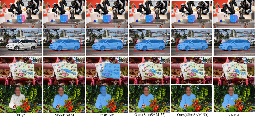
Figure 4: Top 2 rows: segmentation results obtained using box prompts; bottom 2 rows: segmentation results achieved with point prompts.

Embedding Aligning. The pruned encoder $v_{2}$ will learn from the embeddings $E_{v_{1}}$ and final image embedding $T_{v_{1}}$ from the pruned encoder $v_{1}$ to expedite knowledge recovery. Simultaneously, it also compute loss functions based on the final image embedding $t_{v_{0}}$ from the original encoder $v_{0}$ to enhance the precision of knowledge recovery. The total loss function for embedding aligning is defined as:

$$\mathcal{L}_{Emb}=\alpha\cdot(\mathcal{L}_{MSE}(E_{v_{1}},E_{v_{2}})+\mathcal{L}_{MSE}(t_{v_{1}},t_{v_{2}}))$$ (7)

$$+(1-\alpha)\cdot\mathcal{L}_{MSE}(t_{v_{0}},t_{v_{2}}),$$

where the dynamic weight $\alpha$ of $n$th epoch is defined as:

$$\alpha=\left\{\begin{array}[]{lc}\frac{N-n-1}{N}&n<N\\ 0&n>=N\end{array}\right..$$ (8)

The dynamic weight $\alpha$ will progressively diminish to zero as the distillation process unfolds. This transition in the learning objective of distillation gradually shifts from $v_{1}$ to $v_{0}$ contributing to a smoother knowledge recovery. We also set $N=10$ for embedding aligning.

Compared to the conventional structural pruning approaches, our alternate slimming strategy achieves 3.40% and 0.92% increase in MIoU when the pruning ratios are 77% and 50%.

4 Experiments

Table 1: Comparing with other existing SAM compression methods on SA-1B dataset. We report parameter counts, MACs, training cost and Mean Intersection over Union (MIoU) for comprehensive and fair comparision.

Type	Method	Params$\downarrow$	MACs$\downarrow$	Training Data	BatchSize	Training GPUs	Iterations	MIoU$\uparrow$
Original	SAM-H [16]	637M	2733G	11M(100%)	256	256	90k	78.30%
	SAM-L [16]	308M	1312G	11M(100%)	128	128	180k	77.67%
	SAM-B [16]	89.7M	369G	11M(100%)	128	128	180k	73.37%
Compressed	FastSAM-s [47]	11M	37G	220k(2%)	32	8	625K	51.72%
	FastSAM-x [47]	68M	330G	220k(2%)	32	8	625K	64.13%
	MobileSAM [45]	6.1M	37G	100k(1%)	8	1	100k	62.73%
	SlimSAM-50(Ours)	24M	95G	10k(0.1%)	4	1	100k	72.33%
	SlimSAM-77(Ours)	5.7M	21G	10k(0.1%)	4	1	200k	67.40%

Table 2: Comparing with other structural pruning methods. ’Ratio’ signifies the pruning ratio applied to channel-wise groups. Training cost remains consistent for the same pruning ratio.

Ratio	Method	Params$\downarrow$	MACs$\downarrow$	MIoU$\uparrow$
Ratio=0%	SAM-H [16]	637M	2733G	78.30%
	SAM-L [16]	308M	1312G	77.67%
	SAM-B [16]	89.7M	369G	73.37%
Ratio=50%	Scratch Distillation	23.9M	95G	1.63%
	Random Pruning			71.03%
	Magnitude Pruning [9]			69.96%
	Hessian Pruning [20]			71.01%
	Taylor Pruning [27]			71.15%
	SlimSAM-50(Ours)			72.33%
Ratio=77%	Scratch Distillation	5.7M	21G	1.34%
	Random Pruning			62.58%
	Magnitude Pruning [9]			61.60%
	Hessian Pruning [20]			63.56%
	Taylor Pruning [27]			64.26%
	SlimSAM-77(Ours)			67.40%

4.1 Experimental Settings

Implementation Details. Our SlimSAM has been implemented in PyTorch [30] and trained on a single Nvidia Titan RTX GPU using only 0.1% (10,000 images) of the SA-1B [16] dataset. The base model of our pruning and distillation method is SAM-B [16]. The model’s parameters were optimized through the ADAM [15] algorithm with a batch size of 4. Training settings for both bottleneck aligning and embedding aligning are identical. The pruned models undergo distillation with an initial learning rate of $1e^{-4}$, which will be reduced by half if validation performance does not improve for 4 consecutive epochs. The total training duration is 40 epochs for SlimSAM-50 (with a 50% pruning ratio) and 80 epochs for SlimSAM-77 (with a 77% pruning ratio). We exclusively compressed the image encoder while retaining SAM’s original prompt encoder and mask decoder. No additional training tricks are employed.

Evaluation Details. To ensure a fair quantitative evaluation of the compressed SAM models, we compute MIoU between the masks predicted by model and the ground truth masks of SA-1B dataset with the given prompts in annotations. For efficiency evaluation, we provide information on parameter counts and MACs. Additionally, we present details about training data, training iteration and training GPUs for evaluating the training cost. Qualitative comparison of results obtained using point prompts, box prompts, and segment everything prompts are also shown in the following section.

4.2 Comparision and Analysis

Comparing with SOTA SAM compression methods. As depicted in Table 1, we conducted a comprehensive comparison encompassing performance, efficiency, and training costs with other SOTA methods. Our SlimSAM-50 and SlimSAM-77 models achieve a remarkable parameter reduction to only 3.8% (24M) and 0.9% (5.7M)of the original count, while also significantly lowering computational demands to just 3.5% (95G) and 0.8% (21G) MACs, all while maintaining performance levels comparable to the original SAM-H. In contrast to other compressed models, our approach yields substantial performance enhancements while simultaneously achieving greater lightweight and efficiency. SlimSAM-50 and SlimSAM-77 outperform other compressed SAM models with minimum 8% and 3% MIoU improvement. SlimSAM consistently delivers more accurate and detailed segmentation results across various prompts, preserving SAM’s robust segmentation capabilities to the greatest extent. This qualitative superiority over other models is visually evident in Figure 4 and 5. Our approach demonstrates outstanding levels of accuracy and correctness. Furthermore, it is important to note that SlimSAM attains these outstanding results with minimal training data requirements, utilizing only 0.1% of the SA-1B dataset, which is over ten times less than other existing methods.

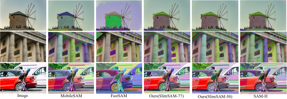
Figure 5: Comparison of segment everything results. In comparison to other models, our segmentation results exhibit greater proximity to the original SAM-H in terms of both accuracy and comprehensiveness.

Comparing with other structural pruning methods. Having demonstrated structural pruning’s efficacy for SAM compression, we established a benchmark for evaluating various pruning methods. We compared with four commonly used methods: random pruning, magnitude pruning, Taylor pruning, and Hessian pruning, each employing different criteria for pruning. Additionally, we conducted comparisons with scratch-distilled models, which are randomly initialized networks sharing the same architecture as the pruned models. To ensure a completely equitable comparison, models with the same pruning ratios were subjected to identical training costs. Table 2 showcases our method’s consistent superiority over other structural pruning techniques, particularly at higher pruning ratios. SlimSAM-50 and SlimSAM-77 outperform alternative methods, achieving a minimum 1% and 3% MIoU improvement while incurring the same training cost. It is noteworthy that the performance of scratch distillation is extremely low at such a limited training cost. This further proves the effectiveness of structural pruning in preserving knowledge from the original model.

5 Ablation Study and Analysis

We conducted a series of ablation experiments on the SA-1B dataset using the SlimSAM-77 model, which features a 77% pruning ratio. To ensure a fair comparison in the ablation experiments, all evaluated models were trained for 40 epochs on 10k images.

Disturbed Taylor Pruning. First, we conducted an ablation study to assess the impact of our proposed disturbed Taylor pruning on distillation. This innovative approach aligns the pruning criteria with the optimization objectives of subsequent distillation, resulting in improved performance recovery. As depicted in Table 3, our disturbed Taylor pruning consistently achieves significantly superior performance at the same training cost. For both the common one-step pruning strategy and our alternate slimming strategy, our method demonstrates MIoU improvements of 0.3% and 0.85% over the original Taylor pruning, respectively.

Intermediate Aligning. We also evaluate the effect of incorporating aligning with intermediate layers into the distillation process. As depicted in Table 4, distilling knowledge from intermediate layers leads to significant improvements in training results. Specifically, learning from bottleneck features and final image embeddings results in a 1.22% MIoU improvement for step 1 distillation, compared to learning solely from image embeddings. Similarly, for step 2 distillation, learning from embedding features and final image embeddings achieves a 0.57% MIoU improvement over the case where learning is based solely on image embeddings.

Table 3: Comparision between proposed disturbed Taylor pruning and original Taylor pruning.

Method	MIoU$\uparrow$
Taylor Pruning	62.04%
Disturbed Taylor Pruning	62.31%
SlimSAM-77 with Taylor Pruning	63.63%
SlimSAM-77 with Disturbed Taylor Pruning	64.48%

Table 4: Effect of distillation from intermediate layers and final output image embeddings.

Step	Distillation Objective	MIoU$\uparrow$
Step 1	Final Image Embeddings	65.10%
Step 1	+ Bottleneck Features	66.32%
Step 2	Final Image Embeddings	63.91%
Step 2	+ Embedding Features	64.48%

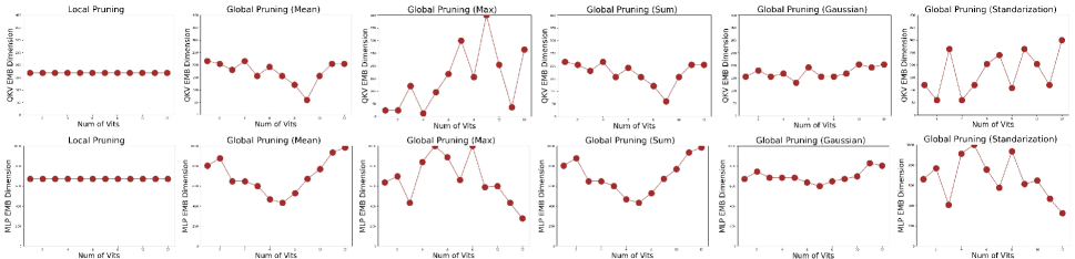
Figure 6: The intermediate dimensions of QVK Attention (top row) and MLP (bottom row) within each ViT after pruning. We present the outcomes of local pruning and global pruning under five distinct normalization methods.

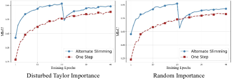
Figure 7: Training results on SA-1B with common one-step strategy and our alternate slimming strategy. Left and right are results with disturbed Taylor importance and random importance.

Alternate Slimming Strategy. In addition, we conducted experiments to investigate the impact of our alternate slimming strategy. Unlike the common one-step pruning strategy, we partition the structural pruning process into two decoupled and progressive steps. In the first step, only the dimensions related to the embedding features are pruned, while in the second stage, only the dimensions related to the bottleneck features are pruned. Following both embedding and bottleneck pruning, knowledge distillation with intermediate layer aligning is employed on the pruned model to recover its performance. For a more exhaustive analysis, we present the results obtained using different pruning criteria to assess whether the effectiveness of our method is influenced by importance estimation. As illustrated in the Figure 7, our alternative slimming strategy yields substantial improvements in MIoU, with gains of 3.9% and 3.5% observed under disturbed Taylor importance estimation and random importance estimation.

Global Pruning vs Local Pruning. Finally, we conducted experiments to evaluate the performance of local pruning and global pruning in bottelneck pruning. Given that the bottleneck dimensions in each block are entirely decoupled, we systematically applied channel-wise group pruning at various ratios for each block while preserving the predefined overall pruning ratio in this step. To obtain a consistent global ranking, we normalized the group importance scores $I_{\mathcal{G}}$ of each layer in five ways: (i) Sum: $I_{\mathcal{G}i}=\frac{I_{\mathcal{G}i}}{\sum_{i=1}^{K}I_{\mathcal{G}i}}$, (ii) Mean: $I_{\mathcal{G}i}=\frac{I_{\mathcal{G}i}}{\sum_{i=1}^{K}I_{\mathcal{G}i}/K}$, (iii) Max: $I_{\mathcal{G}i}=\frac{I_{\mathcal{G}i}}{Max_{i=1}^{K}(I_{\mathcal{G}i})}$, (iv) Standarization: $I_{\mathcal{G}i}=\frac{I_{\mathcal{G}i}-Max_{i=1}^{K}(I_{\mathcal{G}i})}{Max_{i=1}^{K}(I_{\mathcal{G}i})-Min_{i=1}^{K}(I_{\mathcal{G}i})+1e-8}$, (v) Gaussian: $I_{\mathcal{G}i}=\frac{I_{\mathcal{G}i}-\sum_{i=1}^{K}I_{\mathcal{G}i}/K}{\sigma_{i=1}^{K}(I_{\mathcal{G}i})+1e-8}$. As indicated in Table 5, local pruning ensures consistent performance, whereas global pruning raises the model’s upper performance limit. Global pruning’s efficacy is highly dependent on the chosen importance normalization method. For our model, we opted for global pruning with Gaussian normalization, which yielded the best training results. Following global pruning, Figure 6 illustrates the dimensions of bottleneck features (QKV embeddings and MLP hidden embeddings) within each ViT in the image encoder. When applying mean, sum, or Gaussian normalization, the ViTs in the middle exhibit more group redundancy compared to those at the beginning and end. However, the pruned dimensions do not display distinct patterns when utilizing max or standarization normalization.

Table 5: Effect of global pruning evaluated under five different normalization approaches.

Pruning Method	Normlization	MIoU$\uparrow$
Local Pruning	—	64.38%
Global Pruning	Mean	63.64%
	Max	64.35%
	Sum	63.55%
	Gaussian	64.48%
	Standarization	64.14%

6 Conclusion

In this paper, we present an innovative SAM compression method, SlimSAM, which achieves superior performance with minimal training costs. The essence of our approach lies in the efficient reuse of pre-trained SAMs through structural pruning and knowledge distillation, avoiding the need for extensive retraining. We introduce key designs to the compression method for enhancing knowledge retention from the original model. Specifically, our alternate slimming strategy carefully prunes and distills decoupled model structures in an alternating fashion, minimizing any disruptions to the original model. Furthermore, the proposed disturbed Taylor importance estimation rectifies the misalignment between pruning objectives and training targets, thus boosting post-distillation after pruning. SlimSAM convincingly demonstrates its superiority while imposing significantly lower training costs compared to other existing methods. Even when compared with the original SAM-H, our model approaches its performance while achieving an impressive compression ratio. Looking ahead to future research, our framework showcases substantial potential as a general approach for compressing other forthcoming large-scale vision models.

Supplementary Materials

❈ In this document, we provide supplementary materials that extend beyond the scope of the main manuscript, constrained by space limitations. These additional materials include in-depth information about the ablation study of SlimSAM-50, further experiments assessing model efficiency, additional evaluations of training costs, limitation discussion and supplementary qualitative results.

❈ The organizations of this supplementary material are summarized as follows.

$\blacktriangleright$ Sec. A : In Section A, we delve deeper into the ablation study of our SlimSAM-50 model. This section presents extensive experiments that investigate the effects of disturbed Taylor Pruning, the integration of intermediate layer aligning, the impact of alternative slimming strategy, and the efficacy of global pruning across various normalization methods. These comprehensive analyses provide a more nuanced understanding of each technique’s impact on the model’s performance.

$\blacktriangleright$ Sec. B : In Section B, we illustrate the considerable efficacy of our approach in expediting model inference.

$\blacktriangleright$ Sec. C : In addition, we provide detailed insights into the influence of training costs on our SlimSAM framework. We systematically present the training outcomes, comparing the effects of varying amounts of training data and differing numbers of training iterations.

$\blacktriangleright$ Sec. D : Furthermore, we discuss the limitations of our method and the problems need to be solved in the future.

$\blacktriangleright$ Sec. E : Finally, we provide an expanded qualitative comparison to substantiate the superior performance of our proposed model. To illustrate this, we present visualized results obtained using various types of prompts, including point prompts, box prompts, and segment everything prompts.

Appendix A Ablation Study on SlimSAM-50

We performed an extensive series of ablation studies on the SA-1B [16] dataset utilizing the SlimSAM-50 model, characterized by its significant 50% pruning ratio. To guarantee a fair and consistent comparison across these ablation studies, each model under evaluation was uniformly trained over a span of 20 epochs, employing a training dataset comprising 10,000 images.

Table 6: Comparision between proposed disturbed Taylor pruning and original Taylor pruning.

Method	MIoU$\uparrow$
Taylor Pruning	70.02%
Disturbed Taylor Pruning	70.33%
SlimSAM-50 with Taylor Pruning	70.42%
SlimSAM-50 with Disturbed Taylor Pruning	70.81%

Table 7: Effect of distillation from intermediate layers and final output image embeddings.

Step	Distillation Objective	MIoU$\uparrow$
Step 1	Final Image Embeddings	70.86%
Step 1	+ Bottleneck Features	72.07%
Step 2	Final Image Embeddings	70.52%
Step 2	+ Embedding Features	70.81%

Table 8: Effect of global pruning evaluated under five different normalization approaches.

Pruning Method	Normlization	MIoU$\uparrow$
Local Pruning	—	70.81%
Global Pruning	Mean	70.76%
	Max	70.77%
	Sum	70.80%
	Gaussian	70.83%
	Standarization	70.78%

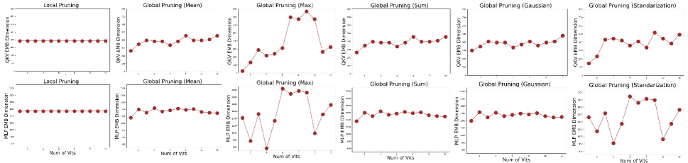
Figure 8: The intermediate dimensions of QVK Attention (top row) and MLP (bottom row) within each ViT after pruning. We present the outcomes of local pruning and global pruning under five distinct normalization methods.

Disturbed Taylor Pruning. Initially, we executed an ablation study to evaluate the effects of our innovative disturbed Taylor pruning technique on distillation processes. This approach strategically aligns pruning criteria with the optimization goals of the ensuing distillation, thereby facilitating enhanced performance recovery. As illustrated in Table 6, our disturbed Taylor pruning method consistently outperforms, achieving markedly better results at equivalent training expenditures. In comparison to the conventional one-step pruning strategy and our alternative slimming approach, our methodology registers MIoU enhancements of 0.31% and 0.39% over the standard Taylor pruning method [27], respectively.

Intermediate Aligning. We further investigated the impact of integrating alignment with intermediate layers in the distillation process. As Table 7 illustrates, leveraging knowledge from these intermediate layers substantially enhances the training outcomes. Specifically, when distillation in step 1 incorporates learning from both bottleneck features and final image embeddings, there is a notable 1.19% improvement in MIoU compared to a methodology reliant solely on image embeddings. Similarly, in step 2 of the distillation process, a strategy that utilizes both embedding features and final image embeddings demonstrates a 0.29% MIoU improvement over approaches exclusively based on image embeddings.

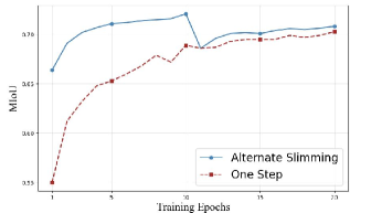
Figure 9: Training results on SA-1B with common one-step strategy and our alternate slimming strategy.

Alternate Slimming Stragtegy. Moreover, we conducted a series of experiments to examine the efficacy of our novel alternate slimming strategy. Diverging from the traditional one-step pruning approach, our method divides the structural pruning into two distinct and progressive phases. In the initial phase, pruning is exclusively focused on the dimensions pertaining to embedding features. The subsequent stage then targets dimensions associated with bottleneck features. After completing both embedding and bottleneck pruning, we employ knowledge distillation with intermediate layer alignment on the pruned model to facilitate performance restoration. The outcomes derived from our proposed disturbed Taylor importance estimation are displayed in Figure 9. This figure demonstrates that our alternative slimming strategy significantly boosts MIoU, achieving an increase of 0.5%. When juxtaposed with the ablation study results of SlimSAM-77, it becomes evident that our strategy exhibits a more pronounced improvement, particularly when applied to models with higher pruning ratios.

Global Pruning vs Local Pruning. In our final set of experiments, we assessed the effectiveness of both local and global pruning approaches in the context of bottleneck pruning. Considering the complete decoupling of bottleneck dimensions in each block, we meticulously implemented channel-wise group pruning at varying ratios across different blocks. This was done while maintaining the predetermined overall pruning ratio for this phase of the study. To obtain a consistent global ranking, we normalized the group importance scores $I_{\mathcal{G}}$ of each layer in five ways: (i) Sum: $I_{\mathcal{G}i}=\frac{I_{\mathcal{G}i}}{\sum_{i=1}^{K}I_{\mathcal{G}i}}$, (ii) Mean: $I_{\mathcal{G}i}=\frac{I_{\mathcal{G}i}}{\sum_{i=1}^{K}I_{\mathcal{G}i}/K}$, (iii) Max: $I_{\mathcal{G}i}=\frac{I_{\mathcal{G}i}}{Max_{i=1}^{K}(I_{\mathcal{G}i})}$, (iv) Standarization: $I_{\mathcal{G}i}=\frac{I_{\mathcal{G}i}-Max_{i=1}^{K}(I_{\mathcal{G}i})}{Max_{i=1}^{K}(I_{\mathcal{G}i})-Min_{i=1}^{K}(I_{\mathcal{G}i})+1e-8}$, (v) Gaussian: $I_{\mathcal{G}i}=\frac{I_{\mathcal{G}i}-\sum_{i=1}^{K}I_{\mathcal{G}i}/K}{\sigma_{i=1}^{K}(I_{\mathcal{G}i})+1e-8}$. Table 8 reveals that while local pruning maintains consistent performance, global pruning enhances the upper limit of the model’s capabilities. In a departure from the findings observed with SlimSAM-77, various normalization methods do not markedly influence post-pruning performance. This suggests that the necessity of selecting an optimal normalization technique increases with the pruning ratio. For our model, we chose global pruning combined with Gaussian normalization, which led to the most favorable training outcomes. Figure 8 delineates the distribution of bottleneck feature dimensions (including QKV and MLP hidden embeddings) across each Vision Transformer (ViT) [6] in the image encoder. When mean, sum, or Gaussian normalization is applied, the dimensions within the ViTs tend to distribute more evenly. However, employing max or standardization normalization often results in significant variances in the intermediate dimensions of each ViT.

Appendix B More Analysis on Efficiency

In the principal manuscript, the high efficiency of our SlimSAM model is objectively substantiated through the disclosure of parameter counts and Multiply-Accumulate Operations (MACs). This section extends the evaluation by reporting on actual acceleration in inference, further affirming the model’s efficiency. As delineated in Table 9, SlimSAM-50 outperforms the original SAM-H model by achieving a 6.9-fold increase in inference speed, while SlimSAM-77 attains an 8.3-fold acceleration. Our compression methodology markedly diminishes the actual inference time, concurrently effecting substantial reductions in both model size and MACs. The inference acceleration metrics were tested using an NVIDIA TITAN RTX GPU.

Table 9: Inference acceleration was empirically tested on an NVIDIA TITAN RTX GPU, revealing that higher pruning rates significantly improve inference speed.

Pruning Ratio	Method	Speed Up$\uparrow$
Ratio=0%	SAM-H [16]	Faster×1.0
	SAM-L [16]	Faster×1.7
	SAM-B [16]	Faster×4.3
Ratio=50%	SlimSAM-50(Ours)	Faster×6.9
Ratio=77%	SlimSAM-77(Ours)	Faster×8.6

Appendix C More Analysis on Training Costs

In our foundational manuscripts, we demonstrate that SlimSAM exhibits exceptional compression performance with minimal training cost. A pertinent inquiry emerges: can SlimSAM maintain its competitive performance with reduced training cost? To address this, we have undertaken supplementary experiments focusing on the interplay between training cost and performance.

In Table 10, we present the results of additional experiments conducted with varying quantities of training data, while keeping the number of training iterations constant. We observe that with a pruning ratio of 50%, a reduction in the volume of training data only marginally impacts the model’s performance. Notably, even when trained with a limited dataset of just 2,000 images, our SlimSAM-50 model remarkably attains an MIoU of nearly 70%. However, as the pruning ratio is elevated to 77%, a decrease in training data more significantly affects performance. This leads to the inference that although our methodology, which integrates pruning and distillation techniques, mitigates the need for extensive training datasets, the availability of more training data can still enhance model performance, particularly at higher pruning rates. It can be anticipated that with an increase in the volume of training data, our model may potentially achieve lossless compression of SAM.

Table 11 showcases the outcomes of experiments conducted by modifying the parameters for training iterations, while maintaining a constant training dataset size. The results clearly illustrate a direct relationship between the quantity of training iterations and the effectiveness of the model compression. It is evident that more extensive training significantly improves the performance of our compressed models. Remarkably, SlimSAM maintains its superiority over other methods even when the training iterations are halved, demonstrating its robustness and efficiency in achieving high-performance compression.

Table 10: The training results were compared using varied amount of training data but maintaining same training iterations.

Pruning Ratio	Training Data	Training Iters	MIoU$\uparrow$
Ratio=50%	10k	100k	72.33%
	5k	100k	71.89%
	2k	100k	69.79%
Ratio=77%	10k	200k	67.40%
	5k	200k	64.47%
	2k	200k	61.72%

Table 11: Training outcomes were evaluated using the same amount of training data across different numbers of training iterations.

Pruning Ratio	Training Data	Training Iters	MIoU$\uparrow$
Ratio=50%	10k	50k	70.83%
	10k	100k	72.33%
Ratio=77%	10k	100k	64.43%
	10k	200k	67.40%

Appendix D Limitations

In this analysis, we critically examine the constraints of our methodology.

First, our approach demonstrates robust compression performance with minimal training data. Nonetheless, an expanded training dataset could further enhance the model’s capabilities. Our current pretrained SlimSAMs, limited by hardware constraints, are trained on a dataset of only 10,000 images from the SA-1B dataset. Utilizing a more comprehensive training dataset could potentially enable our method to achieve lossless compression.

Second, the essence of our method lies in employing structural pruning and knowledge distillation to preserve the knowledge of original pretrained SAMs. This strategy inherently sets the performance ceiling of our model at the level of the original SAM. We found it challenging to surpass the performance of the original SAM, which acted as both the target for pruning and the target for optimization. A key area for future research will be exploring how to surpass the performance of the original SAM with limited parameter counts and reduced training costs.

Appendix E More Qualitative Results

We present more visual comparison with other existing compressed models and the original SAM-H. Figure 10 provides a detailed visual comparison using the segment everything prompt, while Figures 11 and 12 showcase additional qualitative results obtained with box prompts and point prompts, respectively. Relative to established compression models such as MobileSAM [45] and FastSAM [47], our model distinctly outperforms in achieving more precise segmentation, particularly noticeable at the object edges. Notably, even when benchmarked against SAM-H, our model demonstrates commensurate segmentation capabilities.

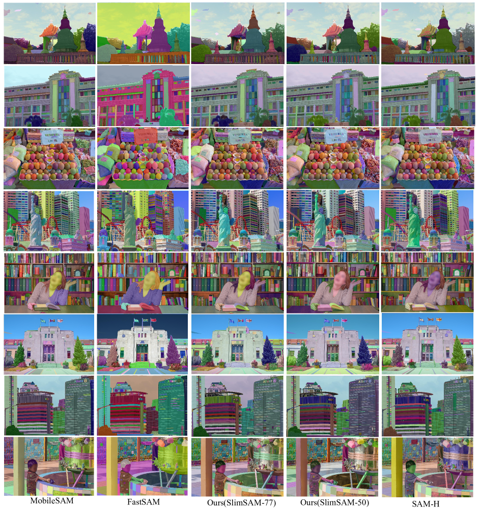
Figure 10: Comparison of segmentation results using segment everything prompts

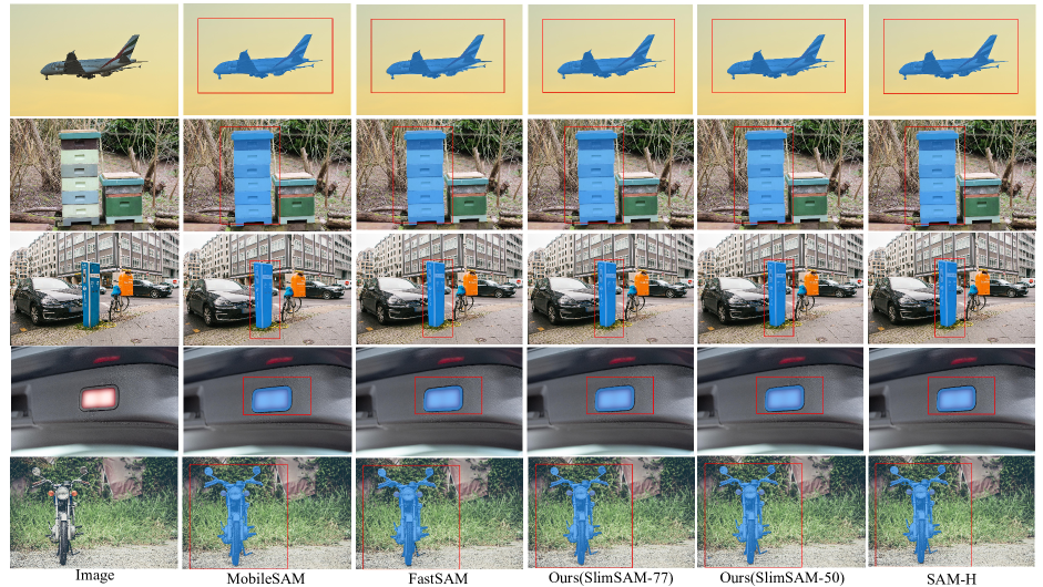
Figure 11: Comparison of segmentation results using box prompts

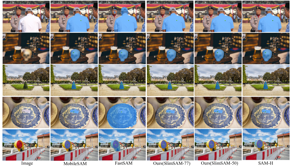
Figure 12: Comparison of segmentation results using point prompts

References

- Chen et al. [2017] Guobin Chen, Wongun Choi, Xiang Yu, Tony Han, and Manmohan Chandraker. Learning efficient object detection models with knowledge distillation. Advances in neural information processing systems, 30, 2017.
- Chen et al. [2023] Keyan Chen, Chenyang Liu, Hao Chen, Haotian Zhang, Wenyuan Li, Zhengxia Zou, and Zhenwei Shi. Rsprompter: Learning to prompt for remote sensing instance segmentation based on visual foundation model. arXiv preprint arXiv:2306.16269, 2023.
- Chin et al. [2020] Ting-Wu Chin, Ruizhou Ding, Cha Zhang, and Diana Marculescu. Towards efficient model compression via learned global ranking. In Proceedings of the IEEE/CVF conference on computer vision and pattern recognition, pages 1518–1528, 2020.
- Ding et al. [2019] Xiaohan Ding, Guiguang Ding, Yuchen Guo, and Jungong Han. Centripetal sgd for pruning very deep convolutional networks with complicated structure. In Proceedings of the IEEE/CVF conference on computer vision and pattern recognition, pages 4943–4953, 2019.
- Dong et al. [2017] Xin Dong, Shangyu Chen, and Sinno Pan. Learning to prune deep neural networks via layer-wise optimal brain surgeon. Advances in neural information processing systems, 30, 2017.
- Dosovitskiy et al. [2020] Alexey Dosovitskiy, Lucas Beyer, Alexander Kolesnikov, Dirk Weissenborn, Xiaohua Zhai, Thomas Unterthiner, Mostafa Dehghani, Matthias Minderer, Georg Heigold, Sylvain Gelly, et al. An image is worth 16x16 words: Transformers for image recognition at scale. arXiv preprint arXiv:2010.11929, 2020.
- Fang et al. [2023] Gongfan Fang, Xinyin Ma, Mingli Song, Michael Bi Mi, and Xinchao Wang. Depgraph: Towards any structural pruning. In Proceedings of the IEEE/CVF Conference on Computer Vision and Pattern Recognition, pages 16091–16101, 2023.
- Frankle and Carbin [2018] Jonathan Frankle and Michael Carbin. The lottery ticket hypothesis: Finding sparse, trainable neural networks. arXiv preprint arXiv:1803.03635, 2018.
- Han et al. [2015] Song Han, Jeff Pool, John Tran, and William Dally. Learning both weights and connections for efficient neural network. Advances in neural information processing systems, 28, 2015.
- He et al. [2017] Yihui He, Xiangyu Zhang, and Jian Sun. Channel pruning for accelerating very deep neural networks. In Proceedings of the IEEE international conference on computer vision, pages 1389–1397, 2017.
- Hinton et al. [2015] Geoffrey Hinton, Oriol Vinyals, and Jeff Dean. Distilling the knowledge in a neural network. arXiv preprint arXiv:1503.02531, 2015.
- Hong et al. [2023] Yining Hong, Haoyu Zhen, Peihao Chen, Shuhong Zheng, Yilun Du, Zhenfang Chen, and Chuang Gan. 3d-llm: Injecting the 3d world into large language models. arXiv preprint arXiv:2307.12981, 2023.
- Jing et al. [2023] Yongcheng Jing, Xinchao Wang, and Dacheng Tao. Segment anything in non-euclidean domains: Challenges and opportunities. arXiv preprint arXiv:2304.11595, 2023.
- Jocher et al. [2023] Glenn Jocher, Ayush Chaurasia, and Jing Qiu. Yolo by ultralytics, 2023.
- Kingma and Ba [2014] Diederik P Kingma and Jimmy Ba. Adam: A method for stochastic optimization. arXiv preprint arXiv:1412.6980, 2014.
- Kirillov et al. [2023] Alexander Kirillov, Eric Mintun, Nikhila Ravi, Hanzi Mao, Chloe Rolland, Laura Gustafson, Tete Xiao, Spencer Whitehead, Alexander C Berg, Wan-Yen Lo, et al. Segment anything. arXiv preprint arXiv:2304.02643, 2023.
- Lee et al. [2019] Namhoon Lee, Thalaiyasingam Ajanthan, Stephen Gould, and Philip HS Torr. A signal propagation perspective for pruning neural networks at initialization. arXiv preprint arXiv:1906.06307, 2019.
- Li et al. [2016] Hao Li, Asim Kadav, Igor Durdanovic, Hanan Samet, and Hans Peter Graf. Pruning filters for efficient convnets. arXiv preprint arXiv:1608.08710, 2016.
- Liang et al. [2022] Weicong Liang, Yuhui Yuan, Henghui Ding, Xiao Luo, Weihong Lin, Ding Jia, Zheng Zhang, Chao Zhang, and Han Hu. Expediting large-scale vision transformer for dense prediction without fine-tuning. Advances in Neural Information Processing Systems, 35:35462–35477, 2022.
- Liu et al. [2021] Liyang Liu, Shilong Zhang, Zhanghui Kuang, Aojun Zhou, Jing-Hao Xue, Xinjiang Wang, Yimin Chen, Wenming Yang, Qingmin Liao, and Wayne Zhang. Group fisher pruning for practical network compression. In International Conference on Machine Learning, pages 7021–7032. PMLR, 2021.
- Liu et al. [2023] Songhua Liu, Jingwen Ye, and Xinchao Wang. Any-to-any style transfer: Making picasso and da vinci collaborate. arXiv e-prints, pages arXiv–2304, 2023.
- Liu et al. [2019] Yifan Liu, Ke Chen, Chris Liu, Zengchang Qin, Zhenbo Luo, and Jingdong Wang. Structured knowledge distillation for semantic segmentation. In Proceedings of the IEEE/CVF conference on computer vision and pattern recognition, pages 2604–2613, 2019.
- Liu et al. [2017] Zhuang Liu, Jianguo Li, Zhiqiang Shen, Gao Huang, Shoumeng Yan, and Changshui Zhang. Learning efficient convolutional networks through network slimming. In Proceedings of the IEEE international conference on computer vision, pages 2736–2744, 2017.
- Lu et al. [2023] Zhihe Lu, Zeyu Xiao, Jiawang Bai, Zhiwei Xiong, and Xinchao Wang. Can sam boost video super-resolution? arXiv preprint arXiv:2305.06524, 2023.
- Ma et al. [2023] Xinyin Ma, Gongfan Fang, and Xinchao Wang. Llm-pruner: On the structural pruning of large language models. arXiv preprint arXiv:2305.11627, 2023.
- Mishra and Marr [2017] Asit Mishra and Debbie Marr. Apprentice: Using knowledge distillation techniques to improve low-precision network accuracy. arXiv preprint arXiv:1711.05852, 2017.
- Molchanov et al. [2019] Pavlo Molchanov, Arun Mallya, Stephen Tyree, Iuri Frosio, and Jan Kautz. Importance estimation for neural network pruning. In Proceedings of the IEEE/CVF conference on computer vision and pattern recognition, pages 11264–11272, 2019.
- Nayak et al. [2019] Gaurav Kumar Nayak, Konda Reddy Mopuri, Vaisakh Shaj, Venkatesh Babu Radhakrishnan, and Anirban Chakraborty. Zero-shot knowledge distillation in deep networks. In International Conference on Machine Learning, pages 4743–4751. PMLR, 2019.
- Park et al. [2020] Sejun Park, Jaeho Lee, Sangwoo Mo, and Jinwoo Shin. Lookahead: A far-sighted alternative of magnitude-based pruning. arXiv preprint arXiv:2002.04809, 2020.
- Paszke et al. [2019] Adam Paszke, Sam Gross, Francisco Massa, Adam Lerer, James Bradbury, Gregory Chanan, Trevor Killeen, Zeming Lin, Natalia Gimelshein, Luca Antiga, et al. Pytorch: An imperative style, high-performance deep learning library. Advances in neural information processing systems, 32, 2019.
- Sanh et al. [2020] Victor Sanh, Thomas Wolf, and Alexander Rush. Movement pruning: Adaptive sparsity by fine-tuning. Advances in Neural Information Processing Systems, 33:20378–20389, 2020.
- Shen et al. [2023] Qiuhong Shen, Xingyi Yang, and Xinchao Wang. Anything-3d: Towards single-view anything reconstruction in the wild. arXiv preprint arXiv:2304.10261, 2023.
- Sun et al. [2019] Siqi Sun, Yu Cheng, Zhe Gan, and Jingjing Liu. Patient knowledge distillation for bert model compression. arXiv preprint arXiv:1908.09355, 2019.
- Tan et al. [2019] Xu Tan, Yi Ren, Di He, Tao Qin, Zhou Zhao, and Tie-Yan Liu. Multilingual neural machine translation with knowledge distillation. arXiv preprint arXiv:1902.10461, 2019.
- Touvron et al. [2023] Hugo Touvron, Thibaut Lavril, Gautier Izacard, Xavier Martinet, Marie-Anne Lachaux, Timothée Lacroix, Baptiste Rozière, Naman Goyal, Eric Hambro, Faisal Azhar, et al. Llama: Open and efficient foundation language models. arXiv preprint arXiv:2302.13971, 2023.
- Wang et al. [2018] Xiaojie Wang, Rui Zhang, Yu Sun, and Jianzhong Qi. Kdgan: Knowledge distillation with generative adversarial networks. Advances in neural information processing systems, 31, 2018.
- Wu et al. [2023] Junde Wu, Rao Fu, Huihui Fang, Yuanpei Liu, Zhaowei Wang, Yanwu Xu, Yueming Jin, and Tal Arbel. Medical sam adapter: Adapting segment anything model for medical image segmentation. arXiv preprint arXiv:2304.12620, 2023.
- Wu et al. [2022] Kan Wu, Jinnian Zhang, Houwen Peng, Mengchen Liu, Bin Xiao, Jianlong Fu, and Lu Yuan. Tinyvit: Fast pretraining distillation for small vision transformers. In European Conference on Computer Vision, pages 68–85. Springer, 2022.
- Xu et al. [2020] Guodong Xu, Ziwei Liu, Xiaoxiao Li, and Chen Change Loy. Knowledge distillation meets self-supervision. In European Conference on Computer Vision, pages 588–604. Springer, 2020.
- Yang et al. [2023a] Huanrui Yang, Hongxu Yin, Maying Shen, Pavlo Molchanov, Hai Li, and Jan Kautz. Global vision transformer pruning with hessian-aware saliency. In Proceedings of the IEEE/CVF Conference on Computer Vision and Pattern Recognition, pages 18547–18557, 2023a.
- Yang et al. [2023b] Jinyu Yang, Mingqi Gao, Zhe Li, Shang Gao, Fangjing Wang, and Feng Zheng. Track anything: Segment anything meets videos. arXiv preprint arXiv:2304.11968, 2023b.
- Yang et al. [2023c] Yunhan Yang, Xiaoyang Wu, Tong He, Hengshuang Zhao, and Xihui Liu. Sam3d: Segment anything in 3d scenes. arXiv preprint arXiv:2306.03908, 2023c.
- You et al. [2019] Zhonghui You, Kun Yan, Jinmian Ye, Meng Ma, and Ping Wang. Gate decorator: Global filter pruning method for accelerating deep convolutional neural networks. Advances in neural information processing systems, 32, 2019.
- Yu et al. [2023] Tao Yu, Runseng Feng, Ruoyu Feng, Jinming Liu, Xin Jin, Wenjun Zeng, and Zhibo Chen. Inpaint anything: Segment anything meets image inpainting. arXiv preprint arXiv:2304.06790, 2023.
- Zhang et al. [2023] Chaoning Zhang, Dongshen Han, Yu Qiao, Jung Uk Kim, Sung-Ho Bae, Seungkyu Lee, and Choong Seon Hong. Faster segment anything: Towards lightweight sam for mobile applications. arXiv preprint arXiv:2306.14289, 2023.
- Zhao et al. [2022] Borui Zhao, Quan Cui, Renjie Song, Yiyu Qiu, and Jiajun Liang. Decoupled knowledge distillation. In Proceedings of the IEEE/CVF Conference on computer vision and pattern recognition, pages 11953–11962, 2022.
- Zhao et al. [2023] Xu Zhao, Wenchao Ding, Yongqi An, Yinglong Du, Tao Yu, Min Li, Ming Tang, and Jinqiao Wang. Fast segment anything. arXiv preprint arXiv:2306.12156, 2023.