A Derived Geometric Approach to Propagation of Solution Singularities for Non-linear PDEs I: Foundations

Jacob Kryczka Jacob Kryczka Beijing Institute of Mathematical Sciences and Applications, A4, Room 209 No. 544, Hefangkou Village, Huaibei Town, Huairou District, Beijing 101408, China jkryczka@bimsa.cn ,ย  Artan Sheshmani Artan Sheshmani Beijing Institute of Mathematical Sciences and Applications, A6, Room 205 No. 544, Hefangkou Village, Huaibei Town, Huairou District, Beijing 101408, China Massachusetts Institute of Technology (MIT), IAiFi Institute, 182 Memorial Drive, Cambridge, MA 02139, USA National Research University, Higher School of Economics, Russian Federation, Laboratory of Mirror Symmetry, NRU HSE, 6 Usacheva Street, Moscow, Russia, 119048 artan@mit.edu ย andย  Shing-Tung Yau Shing-Tung Yau Yau Mathematical Sciences Center, Tsinghua University, Haidian District, Beijing, China Beijing Institute of Mathematical Sciences and Applications, No. 544, Hefangkou Village, Huaibei Town, Huairou District, Beijing 101408, China styau@tsinghua.edu.cn
Abstract.

We construct a sheaf theoretic and derived geometric machinery to study nonlinear partial differential equations and their singular supports. We establish a notion of derived microlocalization for solution spaces of non-linear equations and develop a formalism to pose and solve singular non-linear Cauchy problems globally. Using this approach we estimate the domains of propagation for the solutions of non-linear systems. It is achieved by exploiting the fact that one may greatly enrich and simplify the study of derived non-linear PDEs over a space X๐‘‹X by studying its derived linearization which is a module over the sheaf of functions on the S1superscript๐‘†1S^{1}-equivariant derived loop stack โ„’โ€‹Xโ„’๐‘‹\mathcal{L}X.

Key words and phrases:
Non-linear PDE, Derived Algebraic Geometry, Propagation, Derived Singular Support, Derived Linearization, Derived Microlocalization, Loop Stack.

Introduction

In this paper we formulate and prove a propagation of solution singularities theorem for certain non-linear partial differential equations (๐–ญ๐–ซ๐–ฏ๐–ฃ๐–ค๐—Œ๐–ญ๐–ซ๐–ฏ๐–ฃ๐–ค๐—Œ\mathsf{NLPDEs}) over general classes of not necessarily smooth analytic or algebraic spaces X๐‘‹X using ideas from derived geometry and microlocal sheaf theory. Roughly speaking, this amounts to obtaining cohomological vanishing criteria for certain global solution sheaves on two spaces related to X๐‘‹X, the derived loop stack โ„’โ€‹Xโ„’๐‘‹\mathcal{L}X and the Hodge stack X

Hod

.
subscript๐‘‹

Hod

X_{\scalebox{0.65}{\mbox{$\displaystyle Hod$}}}.
It is obtained via the deformation to the normal bundle construction [GR17b, Sect. 9.2.], and by studying a suitable (โˆž,1)1(\infty,1)-subcategory of ๐–จ๐—‡๐–ฝ๐–ข๐—ˆ๐—โ€‹(โ„’โ€‹X)๐–จ๐—‡๐–ฝ๐–ข๐—ˆ๐—โ„’๐‘‹\mathsf{IndCoh}(\mathcal{L}X) consisting of equivariant ind-coherent sheaves (see [GR17a, GR17b] and [BZN12, TV09]).

We state it now, referring to Sect. 0.1 for a more detailed overview and to Sect. 8 and Sect. 9 for the full treatment and precise formulation.

Consider the (โˆž,1)1(\infty,1)-category of derived analytic (or algebraic) stacks ๐–ฃ๐– ๐—‡๐–ฒ๐—๐—„โ„‚subscript๐–ฃ๐– ๐—‡๐–ฒ๐—๐—„โ„‚\mathsf{DAnStk}_{\mathbb{C}}. For such an object X๐‘‹X the canonical map to its de Rham stack p:Xโ†’Xdโ€‹R:๐‘โ†’๐‘‹subscript๐‘‹๐‘‘๐‘…p:X\rightarrow X_{dR} defines a right-adjoint derived analytic โˆž\infty-jet functor

๐–ฉ๐–พ๐—๐—ŒAโ€‹n,Xโˆžโ€‹(โˆ’):=pโˆ—:๐–ฃ๐– ๐—‡๐–ฒ๐—๐—„โ„‚/Xโ†’๐–ฃ๐– ๐—‡๐–ฒ๐—๐—„โ„‚/Xdโ€‹R,:assignsuperscriptsubscript๐–ฉ๐–พ๐—๐—Œ๐ด๐‘›๐‘‹subscript๐‘โ†’subscript๐–ฃ๐– ๐—‡๐–ฒ๐—๐—„โ„‚๐‘‹subscript๐–ฃ๐– ๐—‡๐–ฒ๐—๐—„โ„‚subscript๐‘‹๐‘‘๐‘…\mathsf{Jets}_{An,X}^{\infty}(-):=p_{*}:\mathsf{DAnStk}_{\mathbb{C}/X}\rightarrow\mathsf{DAnStk}_{\mathbb{C}/X_{dR}},

and one may understand a derived analytic non-linear PDE (Definition 4.66) to be a derived closed substack ๐’ดโ†’๐–ฉ๐–พ๐—๐—ŒAโ€‹n,Xโˆžโ€‹(E),โ†’๐’ดsuperscriptsubscript๐–ฉ๐–พ๐—๐—Œ๐ด๐‘›๐‘‹๐ธ\mathcal{Y}\rightarrow\mathsf{Jets}_{An,X}^{\infty}(E), with corresponding pre-stack of solutions โ„โ€‹๐’ฎโ€‹๐—ˆ๐–ซยฏXโ€‹(๐’ด)โ„subscriptยฏ๐’ฎ๐—ˆ๐–ซ๐‘‹๐’ด{\color[rgb]{0.05,0.05,0.05}\definecolor[named]{pgfstrokecolor}{rgb}{0.05,0.05,0.05}\pgfsys@color@gray@stroke{0.05}\pgfsys@color@gray@fill{0.05}\mathbb{R}\underline{\mathcal{S}\mathsf{oL}}}_{X}(\mathcal{Y}) (Definition 4.38). Under necessary finiteness conditions investigated in this work (the property of being โ€˜๐’Ÿ๐’Ÿ\mathcal{D}-finitaryโ€™ (Definition 7.4)) we are guaranteed the existence of a global dualizable cotangent complex. The dual complex ๐’ฏ๐’ด,subscript๐’ฏ๐’ด\mathcal{T}_{\mathcal{Y}}, is then equipped with a certain (homotopy-coherent) lift via the deformation to the normal bundle construction of the formal moduli problem Xโ†’Xdโ€‹Rโ†’๐‘‹subscript๐‘‹๐‘‘๐‘…X\rightarrow X_{dR}. In the context of Simpsonโ€™s non-abelian Hodge theory [Sim96, Sim09] this is a lift to the Hodge stack X

Hod

subscript๐‘‹

Hod

X_{\scalebox{0.65}{\mbox{$\displaystyle Hod$}}}
. Via this construction, we attribute to ๐’ฏ๐’ดsubscript๐’ฏ๐’ด\mathcal{T}_{\mathcal{Y}} a sheaf of solutions and discuss when it is a perfect complex. Linearizing appropriately around a solution ฯ†๐œ‘\varphi to the NLPDE (Sect. 8) produces a compact object in the category of sheaves over โ„’โ€‹Xโ„’๐‘‹\mathcal{L}X, by the Koszul duality of [BZN12], whereby lifting to X

Hod

subscript๐‘‹

Hod

X_{\scalebox{0.65}{\mbox{$\displaystyle Hod$}}}
and passing to the special fiber yields a perfect complex of sheaves on the cotangent stack ๐–ณโˆ—โ€‹Xsuperscript๐–ณ๐‘‹\mathsf{T}^{*}X. The combination of these steps is called (derived) micro-linearization; the resulting sheaf can be thought of as the associated graded object to a good filtration (as in [Kas95, Kas03] etc.) on the linearization sheaf, denoted by ฮผโ„โ€‹(

T

๐’ด,ฯ†
)
.
superscript๐œ‡โ„subscript

T

๐’ด๐œ‘
{}^{\mathbb{R}}\mu(\scalebox{1.1}{\mbox{$\displaystyle\mathcal{T}$}}_{\mathcal{Y},\varphi}).

Main Theorem. (Thm. 9.19 and Prop. 9.17 , 9.20) Given a derived non-linear PDE ๐’ด๐’ด\mathcal{Y} over a derived scheme X๐‘‹X locally almost of finite type, the microlocalization of its linearization ฮผโ„โ€‹(

T

๐’ด,ฯ†
)
superscript๐œ‡โ„subscript

T

๐’ด๐œ‘
{}^{\mathbb{R}}\mu(\scalebox{1.1}{\mbox{$\displaystyle\mathcal{T}$}}_{\mathcal{Y},\varphi})
along ฯ†๐œ‘\varphi is an object of ๐–จ๐—‡๐–ฝ๐–ข๐—ˆ๐—โ€‹(๐–ณโˆ—โ€‹X),๐–จ๐—‡๐–ฝ๐–ข๐—ˆ๐—superscript๐–ณ๐‘‹\mathsf{IndCoh}(\mathsf{T}^{*}X), with Koszul dual object in ๐–จ๐—‡๐–ฝ๐–ข๐—ˆ๐—โ€‹(โ„’โ€‹X)S1๐–จ๐—‡๐–ฝ๐–ข๐—ˆ๐—superscriptโ„’๐‘‹superscript๐‘†1\mathsf{IndCoh}(\mathcal{L}X)^{S^{1}}. Its support defines the characteristic variety Cโ€‹hฯ†โ€‹(๐’ด)๐ถsubscriptโ„Ž๐œ‘๐’ดCh_{\varphi}(\mathcal{Y}) of ๐’ด.๐’ด\mathcal{Y}. Moreover, if ๐’ด๐’ด\mathcal{Y} is ๐’Ÿ๐’Ÿ\mathcal{D}-finitary and admits deformation theory relative to quasi-smooth X๐‘‹X, so does โ„โ€‹๐’ฎโ€‹๐—ˆ๐–ซยฏXโ€‹(๐’ด)โ„subscriptยฏ๐’ฎ๐—ˆ๐–ซ๐‘‹๐’ด{\color[rgb]{0.05,0.05,0.05}\definecolor[named]{pgfstrokecolor}{rgb}{0.05,0.05,0.05}\pgfsys@color@gray@stroke{0.05}\pgfsys@color@gray@fill{0.05}\mathbb{R}\underline{\mathcal{S}\mathsf{oL}}}_{X}(\mathcal{Y}) and its corresponding derived linearization sheaf is locally constant in non-characteristic directions.

The terminology of the Main Theorem is chosen to draw parallels with several more explicit situations where it is employed throughout this work (namely Theorem A-D). For example, local constancy can be understood more earnestly as a statement on the perfectness of the linearization complex in terms of its singular support as an ind-coherent sheaf on X๐‘‹X (see Theorem D. below). Then, โ€œnon-characteristic directionsโ€ refer to points (z,ฮพ)๐‘ง๐œ‰(z,\xi) not contained within the singular support of the linearization complex.

It is also given in a more explicit context of derived algebraic ๐’Ÿ๐’Ÿ\mathcal{D}-geometry for NLPDEs (see Theorem A below) and it implies the well-posedness of Cauchy problems for NLPDEs with singularities along an initial surface, provided it is non-microcharacteristic for ๐’ด๐’ด\mathcal{Y} (this is Theorem B.)

In this paper we will also treat finiteness questions for NLPDEs over different types of spaces: algebraic, analytic and some of their natural derived enhancements. Specifically, our results hold for derived enhancements of the classical Grothendieck sites (with appropriate รฉtale topologies)

(Aโ€‹fโ€‹fโ„‚,รฉt)โŸAffineย โ€‹โ„‚โˆ’schemes,(Aโ€‹nโ„‚,รฉt)โŸโ„‚โˆ’Analytic spaces,(Aโ€‹fโ€‹fkf.t,รฉt)โŸFinite type affineย โ€‹kโˆ’schemes.subscriptโŸ๐ด๐‘“subscript๐‘“โ„‚รฉtAffineย โ„‚schemessubscriptโŸ๐ดsubscript๐‘›โ„‚รฉtโ„‚Analytic spacessubscriptโŸ๐ด๐‘“superscriptsubscript๐‘“๐‘˜formulae-sequence๐‘“๐‘กรฉtFinite type affineย ๐‘˜schemes\underbrace{(Aff_{\mathbb{C}},\text{\'{e}t})}_{\color[rgb]{0,0,1}\definecolor[named]{pgfstrokecolor}{rgb}{0,0,1}{\text{Affine }\mathbb{C}-\text{schemes}}},\hskip 14.22636pt\underbrace{(An_{\mathbb{C}},\text{\'{e}t})}_{\color[rgb]{0,0,1}\definecolor[named]{pgfstrokecolor}{rgb}{0,0,1}{\mathbb{C}-\text{Analytic spaces}}},\hskip 14.22636pt\underbrace{(Aff_{k}^{f.t},\text{\'{e}t})}_{\color[rgb]{0,0,1}\definecolor[named]{pgfstrokecolor}{rgb}{0,0,1}{\text{Finite type affine }k-\text{schemes}}}.

Our techniques may be applied to treat (โˆž,1)1(\infty,1)-geometric stacks in any of the following sites of interest in derived algebraic geometry:

  1. (1)

    (๐–ฃ๐– ๐–ฟ๐–ฟkalg,รฉt)::superscriptsubscript๐–ฃ๐– ๐–ฟ๐–ฟ๐‘˜algรฉtabsent\big{(}\mathsf{DAff}_{k}^{\mathrm{alg}},\text{\'{e}t}\big{)}: affine derived k๐‘˜k-schemes with their รฉtale topology. Endowed further with a class of ๐๐\mathbf{P} of รฉtale morphisms รฉt defines a geometry and geometric stacks over it are precisely derived Deligne-Mumford stacks ๐–ฃ๐–ฒ๐—๐—„kDโ€‹M:=๐–ฃ๐–ฒ๐—๐—„gโ€‹eโ€‹oโ€‹mโ€‹(๐–ฃ๐– ๐–ฟ๐–ฟkalg,รฉt;รฉt).assignsuperscriptsubscript๐–ฃ๐–ฒ๐—๐—„๐‘˜๐ท๐‘€superscript๐–ฃ๐–ฒ๐—๐—„๐‘”๐‘’๐‘œ๐‘šsuperscriptsubscript๐–ฃ๐– ๐–ฟ๐–ฟ๐‘˜algรฉtรฉt\mathsf{DStk}_{k}^{DM}:=\mathsf{DStk}^{geom}\big{(}\mathsf{DAff}_{k}^{\mathrm{alg}},\text{\'{e}t};\textbf{\'{e}t}\big{)}.

  2. (2)

    Choosing smooth morphisms instead produces another geometry whose geometric stacks are derived Artin stacks ๐–ฃ๐–ฒ๐—๐—„kAโ€‹rโ€‹t.superscriptsubscript๐–ฃ๐–ฒ๐—๐—„๐‘˜๐ด๐‘Ÿ๐‘ก\mathsf{DStk}_{k}^{Art}.

Analogous examples can be considered in the analytic context [PY20] as well:

  1. (1)

    Consider derived Stein spaces ๐–ฃ๐– ๐—‡โ„‚Steinsuperscriptsubscript๐–ฃ๐– ๐—‡โ„‚Stein\mathsf{DAn}_{\mathbb{C}}^{\mathrm{Stein}} with the analytic รฉtale topology and with ๐๐\mathbf{P} the รฉtale morphisms. This defines a geometry whose geometric stacks are derived complex analytic DM-stack ๐–ฃ๐– ๐—‡๐–ฒ๐—๐—„โ„‚Dโ€‹M:=๐–ฃ๐–ฒ๐—๐—„โ€‹(๐–ฃ๐– ๐—‡โ„‚Stein,รฉt;รฉt).assignsuperscriptsubscript๐–ฃ๐– ๐—‡๐–ฒ๐—๐—„โ„‚๐ท๐‘€๐–ฃ๐–ฒ๐—๐—„superscriptsubscript๐–ฃ๐– ๐—‡โ„‚Steinรฉtรฉt\mathsf{DAnStk}_{\mathbb{C}}^{DM}:=\mathsf{DStk}(\mathsf{DAn}_{\mathbb{C}}^{\mathrm{Stein}},\text{\'{e}t};\textbf{\'{e}t}\big{)}.

  2. (2)

    Considering smooth morphisms defines yet another geometry with geometric stacks given by derived โ„‚โ„‚\mathbb{C}-analytic Artin stacks ๐–ฃ๐– ๐—‡๐–ฒ๐—๐—„๐•”Aโ€‹rโ€‹t.superscriptsubscript๐–ฃ๐– ๐—‡๐–ฒ๐—๐—„๐•”๐ด๐‘Ÿ๐‘ก\mathsf{DAnStk}_{\mathbb{c}}^{Art}.

Note that while we generalize and extend several theorems from the linear setting (see [Kas95, Kas03] and [KO77] and references therein) to provide a first systematic approach to developing a brave new algebraic analysis,111We use this amusing term to mimic that of B. Tรถen and G.Vezzosi who referred to derived algebraic geometry as โ€˜brave new algebraic geometryโ€™ [TV08]. in the setting of derived geometry, we emphasize that we are using the language of (filtered) crystals [GR17b, GR11] as the analog of (filtered) ๐’Ÿ๐’Ÿ\mathcal{D}-modules. This notion is known to be insensitive to the derived structure on X.๐‘‹X. If one wishes to capture this phenomena, a better notion is that of derived ๐’Ÿ๐’Ÿ\mathcal{D}-modules (see for example [Ber21, Def. 4.2.9]).

0.1. Overview and description of the main results

Consider a system of N๐‘N non-linear PDEs imposed on a vector-valued function u=(u1,โ€ฆ,um)๐‘ขsuperscript๐‘ข1โ€ฆsuperscript๐‘ข๐‘šu=(u^{1},\ldots,u^{m}) of variables x=(x1,โ€ฆ,xn)๐‘ฅsubscript๐‘ฅ1โ€ฆsubscript๐‘ฅ๐‘›x=(x_{1},\ldots,x_{n}) given by

(0.1) {๐–ฅ1โ€‹(x1,โ€ฆ,xn,u1,โ€ฆ,um,โ€ฆ,uฯƒฮฑ,โ€ฆ)=0,โ€ฆ๐–ฅNโ€‹(x1,โ€ฆ,xn,u1,โ€ฆ,um,โ€ฆ,uฯƒฮฑ,โ€ฆ)=0,casessubscript๐–ฅ1subscript๐‘ฅ1โ€ฆsubscript๐‘ฅ๐‘›superscript๐‘ข1โ€ฆsuperscript๐‘ข๐‘šโ€ฆsuperscriptsubscript๐‘ข๐œŽ๐›ผโ€ฆ0otherwiseโ€ฆotherwisesubscript๐–ฅ๐‘subscript๐‘ฅ1โ€ฆsubscript๐‘ฅ๐‘›superscript๐‘ข1โ€ฆsuperscript๐‘ข๐‘šโ€ฆsuperscriptsubscript๐‘ข๐œŽ๐›ผโ€ฆ0otherwise\begin{cases}\mathsf{F}_{1}\big{(}x_{1},\ldots,x_{n},u^{1},\ldots,u^{m},\ldots,u_{\sigma}^{\alpha},\ldots\big{)}=0,\\ \ldots\\ \mathsf{F}_{N}\big{(}x_{1},\ldots,x_{n},u^{1},\ldots,u^{m},\ldots,u_{\sigma}^{\alpha},\ldots\big{)}=0,\end{cases}

with ฯƒ๐œŽ\sigma a multi-index and uฯƒฮฑ:=โˆ‚xฯƒuฮฑ,ฮฑ=1,โ€ฆ,m.formulae-sequenceassignsuperscriptsubscript๐‘ข๐œŽ๐›ผsuperscriptsubscript๐‘ฅ๐œŽsuperscript๐‘ข๐›ผ๐›ผ1โ€ฆ๐‘šu_{\sigma}^{\alpha}:=\partial_{x}^{\sigma}u^{\alpha},\alpha=1,\ldots,m. One may think of u๐‘ขu as a section of a trivial rank m๐‘šm vector bundle Eโ†’Xโ†’๐ธ๐‘‹E\rightarrow X. The traditional geometric theory of NLPDEs in the spirit of [VKL86] (see also [KV11] for a comprehensive account) studies (0.1) in terms of an associated geometric object - an appropriate sub-manifold โ„ฐโˆžsuperscriptโ„ฐ\mathcal{E}^{\infty} of an ambient space Jetsโˆžโ€‹(n,m)superscriptJets๐‘›๐‘š\mathrm{Jets}^{\infty}(n,m) of infinite jets in n๐‘›n independent and m๐‘šm dependent variables.

We say we are in the algebraic (resp. analytic) setting when the functions ๐–ฅisubscript๐–ฅ๐‘–\mathsf{F}_{i} are algebraic (resp. analytic) and in either case one obtains โ„ฐโˆžsuperscriptโ„ฐ\mathcal{E}^{\infty} using the formal theory of PDEs and E. Cartanโ€™s tool of prolongation [Kur57] by successively differentiating the ideal of relations. Equivalently, it means the ideal โ„โ„\mathcal{I} is stable under an action by differential operators ๐’ŸXโˆ™โ„โŠ‚โ„โˆ™subscript๐’Ÿ๐‘‹โ„โ„\mathcal{D}_{X}\bullet\hskip 1.42262pt\mathcal{I}\subset\mathcal{I}, defined through a canonical involutive distribution ๐’ž๐’ž\mathcal{C} on jets (see Sect. 3 for details).

Functions on โ„ฐโˆžsuperscriptโ„ฐ\mathcal{E}^{\infty} are modeled by quotient algebras โ„ฌโ„ฌ\mathcal{B} of functions on jets ๐’œ:=๐’ชโ€‹(Jetsโˆžโ€‹(n,m))assign๐’œ๐’ชsuperscriptJets๐‘›๐‘š\mathcal{A}:=\mathcal{O}\big{(}\mathrm{Jets}^{\infty}(n,m)\big{)} by ideals โ„โ„\mathcal{I},

(0.2) โ„โ†’๐’œโ†’๐—‰โ„ฌ.โ†’โ„๐’œ๐—‰โ†’โ„ฌ\mathcal{I}\rightarrow\mathcal{A}\xrightarrow{\mathsf{p}}\mathcal{B}.

A ubiquitous scenario is when โ„ฌโ„ฌ\mathcal{B} is differentially generated i.e. has generic ideal

โ„={ฯˆโˆˆ๐’œ|ฯˆ=โˆ‘i=1,|ฯƒ|โ‰ฅ0Nฯˆi,ฯƒโ€‹(x,u,โˆ‚xฯ„u)โ€‹Dฯƒโ€‹(๐–ฅi),ฯˆi,ฯƒโˆˆ๐’œ},โ„conditional-set๐œ“๐’œformulae-sequence๐œ“superscriptsubscriptformulae-sequence๐‘–1๐œŽ0๐‘subscript๐œ“๐‘–๐œŽ๐‘ฅ๐‘ขsuperscriptsubscript๐‘ฅ๐œ๐‘ขsubscript๐ท๐œŽsubscript๐–ฅ๐‘–subscript๐œ“๐‘–๐œŽ๐’œ\mathcal{I}=\big{\{}\psi\in\mathcal{A}|\psi=\sum_{i=1,|\sigma|\geq 0}^{N}\psi_{i,\sigma}(x,u,\partial_{x}^{\tau}u)D_{\sigma}(\mathsf{F}_{i}),\psi_{i,\sigma}\in\mathcal{A}\big{\}},

where ๐’ŸXโˆ™(๐–ฅi):=Dฯƒโ€‹(๐–ฅi)assignโˆ™subscript๐’Ÿ๐‘‹subscript๐–ฅ๐‘–subscript๐ท๐œŽsubscript๐–ฅ๐‘–\mathcal{D}_{X}\bullet(\mathsf{F}_{i}):=D_{\sigma}(\mathsf{F}_{i}) is the ๐’ŸXsubscript๐’Ÿ๐‘‹\mathcal{D}_{X}-action, or when it is given by non-linear operators locally of Cauchy-Kovalevskaya type (equation 3.7).

Sequences (0.2) define a NLPDE and the geometry of the corresponding solution space ๐–ฒ๐—ˆ๐—…โ€‹(โ„ฌ)๐–ฒ๐—ˆ๐—…โ„ฌ\mathsf{Sol}(\mathcal{B}) encodes not only systems (0.1) but also those systems modulo symmetries. This situation is typical for studying moduli spaces of solutions in gauge theories of the form [[๐–ฒ๐—ˆ๐—…โ€‹(โ„ฌ)/๐’ข]]delimited-[]delimited-[]๐–ฒ๐—ˆ๐—…โ„ฌ๐’ข[\![\mathsf{Sol}(\mathcal{B})/\mathcal{G}]\!] i.e. after one has taken the quotient by the gauge group ๐’ข๐’ข\mathcal{G} of the theory (see Example 4.30).

The linearization of the derived ๐–ญ๐–ซ๐–ฏ๐–ฃ๐–ค๐–ญ๐–ซ๐–ฏ๐–ฃ๐–ค\mathsf{NLPDE} system is, roughly speaking, given by the tangent complex ๐•‹Solโ€‹(โ„ฌ)subscript๐•‹Solโ„ฌ\mathbb{T}_{\mathrm{Sol}(\mathcal{B})} and it turns out we can simltaneously enrich and simplify our study of non-linear PDEs (0.2) by viewing ๐•‹๐–ฒ๐—ˆ๐—…โ€‹(โ„ฌ)subscript๐•‹๐–ฒ๐—ˆ๐—…โ„ฌ\mathbb{T}_{\mathsf{Sol}(\mathcal{B})} as a module not over a non-commutative ring such as ๐’ŸXsubscript๐’Ÿ๐‘‹\mathcal{D}_{X}, but a commutative one - the ring of holomorphic functions ๐’ชโ€‹(โ„’โ€‹X)๐’ชโ„’๐‘‹\mathcal{O}(\mathcal{L}X) on the S1superscript๐‘†1S^{1}-equivariant derived loop stack โ„’โ€‹Xโ„’๐‘‹\mathcal{L}X. From the perspective of derived geometry, ๐•‹๐–ฒ๐—ˆ๐—…โ€‹(โ„ฌ)subscript๐•‹๐–ฒ๐—ˆ๐—…โ„ฌ\mathbb{T}_{\mathsf{Sol}(\mathcal{B})} is computed as an appropriate dual of the cotangent complex ๐•ƒ๐’ฌโˆ™subscript๐•ƒsuperscript๐’ฌโˆ™\mathbb{L}_{\mathcal{Q}^{\bullet}} of a cofibrant resolution ๐’ฌ๐’ฌ\mathcal{Q} of ๐’œ/โ„=โ„ฌ๐’œโ„โ„ฌ\mathcal{A}/\mathcal{I}=\mathcal{B} as a differential graded ๐’œโˆ’๐’Ÿ๐’œ๐’Ÿ\mathcal{A}-\mathcal{D}-algebra.

If X๐‘‹X is no longer smooth, but rather a quasi-smooth derived scheme, we impose a condition on derived analytic and algebraic PDEs ๐’ด๐’ด\mathcal{Y} which assure finite dimensionality of linearized solution spaces. We call it ๐’Ÿ๐’Ÿ\mathcal{D}-Fredholmness (Subsect. 9.2) and roughly speaking, it ensures locally finite presentation of solution spaces to linearizations ๐•‹๐’ดsubscript๐•‹๐’ด\mathbb{T}_{\mathcal{Y}} along solutions, whose underlying linear differential operator will be Fredholm in the usual sense.

The first result treats propagation for ๐–ญ๐–ซ๐–ฏ๐–ฃ๐–ค๐—Œ๐–ญ๐–ซ๐–ฏ๐–ฃ๐–ค๐—Œ\mathsf{NLPDEs} and Cauchy problems for NLPDEs with holomorphic coefficients in the complex domain where the initial data may have singularities along a regular hypersurface on the initial surface.222In the linear setting Y. Hamada [Ham69] shows that by assuming the characteristic surfaces issuing from the points of singularity in the initial data are simple, the singularity in the initial data is propagated along these surfaces. If the initial data have at most poles (resp. essential singularities), the solution in general has at most poles (resp. essential singularities) on these surfaces. To reach it, we overcome the challenges of: (a) building a theory of solution spaces for NLPDEs in the presence of symmetries, (b) finding the correct definitions for their singular supports, here the 111-microcharacteristic variety Cโ€‹hโ€‹aโ€‹r๐’Ÿ1โ€‹(๐’œ)๐ถโ„Ž๐‘Žsuperscriptsubscript๐‘Ÿ๐’Ÿ1๐’œChar_{\mathcal{D}}^{1}(\mathcal{A}) (Subsect.5.2.1 ) and (c) study microlocalization in the non-linear setting.

Theorem A.โ€… Let M๐‘€M be a real analytic manifold with complexification X๐‘‹X and consider a system of non-linear PDEs over X๐‘‹X defined by a sequence (0.2) whose derived space of solutions ๐–ฒ๐—ˆ๐—…Xโ€‹(โ„ฌX)subscript๐–ฒ๐—ˆ๐—…๐‘‹subscriptโ„ฌ๐‘‹\mathsf{Sol}_{X}(\mathcal{B}_{X}) is homotopically finite and admits a globally defined perfect tangent complex ๐•‹โ„ฌ.subscript๐•‹โ„ฌ\mathbb{T}_{\mathcal{B}}. Let VโŠ‚Tโˆ—โ€‹X๐‘‰superscript๐‘‡๐‘‹V\subset T^{*}X be a closed subset and TVโ€‹Tโˆ—โ€‹Xsubscript๐‘‡๐‘‰superscript๐‘‡๐‘‹T_{V}T^{*}X the normal bundle. Then the 111-micro-characteristic variety Cโ€‹hโ€‹aโ€‹r๐’Ÿ,V1โ€‹(โ„ฌ)๐ถโ„Ž๐‘Žsuperscriptsubscript๐‘Ÿ๐’Ÿ๐‘‰1โ„ฌChar_{\mathcal{D},V}^{1}(\mathcal{B}) is a conic subset of ๐–ฒ๐—ˆ๐—…โ€‹(๐’œ)ร—XTVโ€‹Tโˆ—โ€‹X.subscript๐‘‹๐–ฒ๐—ˆ๐—…๐’œsubscript๐‘‡๐‘‰superscript๐‘‡๐‘‹\mathsf{Sol}(\mathcal{A})\times_{X}T_{V}T^{*}X. If V=TXโˆ—โ€‹X,๐‘‰superscriptsubscript๐‘‡๐‘‹๐‘‹V=T_{X}^{*}X, then for all (infinite jets) of solutions ฯ†๐œ‘\varphi of ๐–ฒ๐—ˆ๐—…Xโ€‹(โ„ฌX)subscript๐–ฒ๐—ˆ๐—…๐‘‹subscriptโ„ฌ๐‘‹\mathsf{Sol}_{X}(\mathcal{B}_{X}), by linearization (Prop. 4.39 and Sect. 8) and considering base-change of microfunctions from ๐’ชXโ€‹[๐’ŸX]subscript๐’ช๐‘‹delimited-[]subscript๐’Ÿ๐‘‹\mathcal{O}_{X}[\mathcal{D}_{X}]-modules to โ„ฌXโ€‹[โ„ฐX]subscriptโ„ฌ๐‘‹delimited-[]subscriptโ„ฐ๐‘‹\mathcal{B}_{X}[\mathcal{E}_{X}]-modules, one has that

(0.3) supp(R๐–ฒ๐—ˆ๐—…โ„ฌXโ€‹[โ„ฐX](โ„ฌฮผ(๐•‹โ„ฌโ„“),indโ„ฌXโ€‹[โ„ฐX](๐’žM))โŠ‚Char(โ„ฌฮผ๐•‹โ„ฌ,ฯ†โ„“)โˆฉTMโˆ—X.supp\big{(}R\mathsf{Sol}_{\mathcal{B}_{X}[\mathcal{E}_{X}]}\big{(}_{\mathcal{B}}\mu(\mathbb{T}_{\mathcal{B}}^{\ell}),\mathrm{ind}_{\mathcal{B}_{X}[\mathcal{E}_{X}]}(\mathcal{C}_{M})\big{)}\subset Char\big{(}_{\mathcal{B}}\mu\mathbb{T}_{\mathcal{B},\varphi}^{\ell}\big{)}\cap T_{M}^{*}X.

This result is given in terms of the intersection of the microsupport ฮผโ€‹sโ€‹uโ€‹pโ€‹p๐œ‡๐‘ ๐‘ข๐‘๐‘\mu supp with the zero section of the cotangent bundle. In Sect. 5.2.1 and Sect. 5.4 we give it directly in terms of the 111-microlocalization of ๐•‹โ„ฌsubscript๐•‹โ„ฌ\mathbb{T}_{\mathcal{B}} and for more general V๐‘‰V than the zero-section Lagrangian sub-manifold.

Corollary A.1 If ๐–ฒ๐—ˆ๐—…Xโ€‹(โ„ฌX)subscript๐–ฒ๐—ˆ๐—…๐‘‹subscriptโ„ฌ๐‘‹\mathsf{Sol}_{X}(\mathcal{B}_{X}) is homotopically ๐’ŸXsubscript๐’Ÿ๐‘‹\mathcal{D}_{X}-finitely presented (Sect. 4), then for all solutions ฯ†๐œ‘\varphi to this system, ฮผโ€‹sโ€‹uโ€‹pโ€‹pโ€‹(Rโ€‹๐–ฒ๐—ˆ๐—…Xlโ€‹iโ€‹nโ€‹(ฯ†๐–จ๐—‡๐–ฝ๐–ข๐—ˆ๐—โˆ—โ€‹๐•‹๐–ฒ๐—ˆ๐—…Xโ€‹(โ„ฌ)))=Cโ€‹hโ€‹aโ€‹rโ€‹(ฯ†๐–จ๐—‡๐–ฝ๐–ข๐—ˆ๐—โˆ—โ€‹๐•‹๐–ฒ๐—ˆ๐—…Xโ€‹(โ„ฌ)),๐œ‡๐‘ ๐‘ข๐‘๐‘๐‘…superscriptsubscript๐–ฒ๐—ˆ๐—…๐‘‹๐‘™๐‘–๐‘›superscriptsubscript๐œ‘๐–จ๐—‡๐–ฝ๐–ข๐—ˆ๐—subscript๐•‹subscript๐–ฒ๐—ˆ๐—…๐‘‹โ„ฌ๐ถโ„Ž๐‘Ž๐‘Ÿsuperscriptsubscript๐œ‘๐–จ๐—‡๐–ฝ๐–ข๐—ˆ๐—subscript๐•‹subscript๐–ฒ๐—ˆ๐—…๐‘‹โ„ฌ\mu supp\big{(}R\mathsf{Sol}_{X}^{lin}(\varphi_{\mathsf{IndCoh}}^{*}\mathbb{T}_{\mathsf{Sol}_{X}(\mathcal{B})}\big{)}\big{)}=Char(\varphi_{\mathsf{IndCoh}}^{*}\mathbb{T}_{\mathsf{Sol}_{X}(\mathcal{B})}), where Rโ€‹๐–ฒ๐—ˆ๐—…Xlโ€‹iโ€‹n๐‘…superscriptsubscript๐–ฒ๐—ˆ๐—…๐‘‹๐‘™๐‘–๐‘›R\mathsf{Sol}_{X}^{lin} is the usual linear solution sheaf (Sect. 1).

This follows since homotopically ๐’Ÿ๐’Ÿ\mathcal{D}-finitely presented spaces have a perfect tangent complex that is written as a complex of free โ„ฌโ€‹[๐’ŸX]โ„ฌdelimited-[]subscript๐’Ÿ๐‘‹\mathcal{B}[\mathcal{D}_{X}]-modules of finite rank (Proposition 6.1). Actually, โ„ฌโ„ฌ\mathcal{B} is a compact object, so is a retract of finite cell objects [Kry21, Prop. 8.0.40] and it suffices to consider free algebras ๐–ฅ๐—‹๐–พ๐–พ๐’Ÿโ€‹(โ„ณ)subscript๐–ฅ๐—‹๐–พ๐–พ๐’Ÿโ„ณ\mathsf{Free}_{\mathcal{D}}(\mathcal{M}) on compact ๐’Ÿ๐’Ÿ\mathcal{D}-modules. Pull-back along ฯ†๐œ‘\varphi presents ๐•‹๐–ฒ๐—ˆ๐—…Xโ€‹(โ„ฌ)subscript๐•‹subscript๐–ฒ๐—ˆ๐—…๐‘‹โ„ฌ\mathbb{T}_{\mathsf{Sol}_{X}(\mathcal{B})} as a compact ๐’Ÿ๐’Ÿ\mathcal{D}-module. In particular we have an induced good filtration (over its classical locus) (Proposition 6.2).

One then has the ๐’Ÿ๐’Ÿ\mathcal{D}-algebraic analog (see [Pau22]) of Nirenbergโ€™s formulation of the classical real analytic non-linear Cauchy problem [Nir72].

Theorem B. (Theorem 5.27) Let (๐–ฒ๐—ˆ๐—…Yโ€‹(โ„ฌY),ฯ†)subscript๐–ฒ๐—ˆ๐—…๐‘Œsubscriptโ„ฌ๐‘Œ๐œ‘(\mathsf{Sol}_{Y}(\mathcal{B}_{Y}),\varphi) be as in Theorem A, consider a morphism f:Xโ†’Y:๐‘“โ†’๐‘‹๐‘Œf:X\rightarrow Y of complex analytic manifolds and denote by CVโ€‹(S)subscript๐ถ๐‘‰๐‘†C_{V}(S) the normal cone to SโŠ‚Tโˆ—โ€‹Y๐‘†superscript๐‘‡๐‘ŒS\subset T^{*}Y along a subset V๐‘‰V (see Subsect. 1). Suppose that ฯ€ฬŠXโˆ’1โ€‹(p)โˆฉCTYโˆ—โ€‹Yโ€‹(Cโ€‹hโ€‹aโ€‹rTYโˆ—โ€‹Y1โ€‹(ฯ†โˆ—โ€‹๐•‹โ„ฌ))=โˆ…,superscriptsubscriptฬŠ๐œ‹๐‘‹1๐‘subscript๐ถsuperscriptsubscript๐‘‡๐‘Œ๐‘Œ๐ถโ„Ž๐‘Žsuperscriptsubscript๐‘Ÿsuperscriptsubscript๐‘‡๐‘Œ๐‘Œ1superscript๐œ‘subscript๐•‹โ„ฌ\mathring{\pi}_{X}^{-1}(p)\cap C_{T_{Y}^{*}Y}\big{(}Char_{T_{Y}^{*}Y}^{1}(\varphi^{*}\mathbb{T}_{\mathcal{B}})\big{)}=\emptyset, for all pโˆˆTYโˆ—โ€‹Y๐‘superscriptsubscript๐‘‡๐‘Œ๐‘Œp\in T_{Y}^{*}Y with ฯ€ฬŠX:TฬŠXโˆ—โ€‹Yร—YTYโˆ—โ€‹Yโ†’TYโˆ—โ€‹Y:subscriptฬŠ๐œ‹๐‘‹โ†’subscript๐‘ŒsuperscriptsubscriptฬŠ๐‘‡๐‘‹๐‘Œsuperscriptsubscript๐‘‡๐‘Œ๐‘Œsuperscriptsubscript๐‘‡๐‘Œ๐‘Œ\mathring{\pi}_{X}:\mathring{T}_{X}^{*}Y\times_{Y}T_{Y}^{*}Y\rightarrow T_{Y}^{*}Y, where TฬŠXโˆ—โ€‹YsuperscriptsubscriptฬŠ๐‘‡๐‘‹๐‘Œ\mathring{T}_{X}^{*}Y denotes the removal of the zero-section. Then the natural morphism fโˆ’1โ€‹๐–ฒ๐—ˆ๐—…Yโ€‹(โ„ฌY)โ†’๐–ฒ๐—ˆ๐—…Xโ€‹(Lโ€‹fโˆ—โ€‹โ„ฌY),โ†’superscript๐‘“1subscript๐–ฒ๐—ˆ๐—…๐‘Œsubscriptโ„ฌ๐‘Œsubscript๐–ฒ๐—ˆ๐—…๐‘‹๐ฟsuperscript๐‘“subscriptโ„ฌ๐‘Œf^{-1}\mathsf{Sol}_{Y}(\mathcal{B}_{Y})\rightarrow\mathsf{Sol}_{X}(Lf^{*}\mathcal{B}_{Y}), is an isomorphism.

In this work we develop the tools necessary to formulate Theorem B in a wider context sufficient treat singular non-linear Cauchy problems, for example, those of the form

(0.4) {โˆ‚Lโˆ‚tLโ€‹uฮฑ=๐–ฅโ€‹(t,x,uฮฑ,โˆ‚xฯƒโˆ‚tjuฮฑ),|ฯƒ|+jโ‰คL,j<Lโˆ‚kโˆ‚tkโ€‹uฮฑ|t=0=ฮฆkโ€‹(x),k=0,1,โ€ฆ,mโˆ’1,casesformulae-sequencesuperscript๐ฟsuperscript๐‘ก๐ฟsuperscript๐‘ข๐›ผ๐–ฅ๐‘ก๐‘ฅsuperscript๐‘ข๐›ผsuperscriptsubscript๐‘ฅ๐œŽsuperscriptsubscript๐‘ก๐‘—superscript๐‘ข๐›ผformulae-sequence๐œŽ๐‘—๐ฟ๐‘—๐ฟotherwiseotherwiseotherwiseformulae-sequenceevaluated-atsuperscript๐‘˜superscript๐‘ก๐‘˜superscript๐‘ข๐›ผ๐‘ก0subscriptฮฆ๐‘˜๐‘ฅ๐‘˜01โ€ฆ๐‘š1otherwise\begin{cases}\frac{\partial^{L}}{\partial t^{L}}u^{\alpha}=\mathsf{F}\big{(}t,x,u^{\alpha},\partial_{x}^{\sigma}\partial_{t}^{j}u^{\alpha}\big{)},\hskip 5.69054pt|\sigma|+j\leq L,j<L\\ \\ \frac{\partial^{k}}{\partial t^{k}}u^{\alpha}\big{|}_{t=0}=\Phi_{k}(x),\hskip 5.69054ptk=0,1,\ldots,m-1,\end{cases}

imposed on complex analytic functions uฮฑโ€‹(t,x),ฮฑ=1,โ€ฆ,mformulae-sequencesuperscript๐‘ข๐›ผ๐‘ก๐‘ฅ๐›ผ1โ€ฆ๐‘šu^{\alpha}(t,x),\alpha=1,\ldots,m where for xโˆˆUโŠ‚โ„‚n๐‘ฅ๐‘ˆsuperscriptโ„‚๐‘›x\in U\subset\mathbb{C}^{n} where U๐‘ˆU is an open subset, and tโˆˆโ„๐‘กโ„t\in\mathbb{R}, where ๐–ฅ๐–ฅ\mathsf{F} depends on the derivatives of u๐‘ขu with respect to x,t๐‘ฅ๐‘กx,t of order โ‰คL,absent๐ฟ\leq L, and where we allow ฮฆkโ€‹(x)subscriptฮฆ๐‘˜๐‘ฅ\Phi_{k}(x) to be singular functions. We refer to Subsect. 2.2 for further motivations and Sect. 5.2.1 for details.

Natural generalizations of Theorem B are possible, but then the distinction between the algebraic and analytic (or even Cโˆžsuperscript๐ถC^{\infty}) settings becomes crucial. Namely, we may pass to situations where the functions ๐–ฅ๐–ฅ\mathsf{F} defining our equations are defined over generalized X๐‘‹X which may be singular or perhaps of a higher geometric nature e.g. (derived) stacks. This generalization requires reformulating our affine derived solution spaces ๐–ฒ๐—ˆ๐—…โ€‹(โ„ฌ)๐–ฒ๐—ˆ๐—…โ„ฌ\mathsf{Sol}(\mathcal{B}) in terms of suitable โˆž\infty-topoi of derived stacks in a given geometry. For instance, to treat holomorphic systems we need derived analytic geometry [PY20] while treating Cโˆžsuperscript๐ถC^{\infty}-functions ๐–ฅ๐–ฅ\mathsf{F} requires derived differential geometry - an appropriate environment for studying derived moduli spaces to elliptic NLPDEs arising in symplectic topology and gauge theories [Cos11].

Additional (functional) conditions will then be required, depending on the class of operators under consideration. Indeed, even in the linear setting passing from Cauchy problems for hyperbolic operators with values in hyperfunctions to other functional spaces like distributions requires additional analytic conditions e.g. the operator should have real constant multiplicities. Such analytic conditions can be replaced by geometric conditions on the supports e.g. the characteristic variety is contained in a complexification of a regular involutive submanifold of the conormal bundle to the real ambient manifold (Example 2.13).

The results obtained in this work (Sect. 5.1 and 7) give a flexible derived-geometric framework for studying similar analytic conditions for non-linear systems. Treating these types of questions is outside the scope of the current paper and will be addressed elsewhere.

A final generalization we provide allows us to consider NLPDEs over singular X.๐‘‹X. We consider X๐‘‹X as either a QCA stack [DG13] i.e. quasi-compact with affine diagonal whose underived inertia stack is finitely presented over the underlying classical prestack Xcโ€‹l,superscript๐‘‹๐‘๐‘™{}^{cl}X, a quasi-smooth scheme, or an ind-inf-scheme [GR17b, Chapter 3] (recalled in 1.2). The latter include derived schemes of finite type or locally almost of finite type (hereafter โ€˜laftโ€™) as well as ind-schemes built by gluing laft schemes along closed embeddings. These also include quotients of laft spaces X๐‘‹X by Lie algebroids.

In these situations we typically will not have sheaves of differential operators ๐’ŸXsubscript๐’Ÿ๐‘‹\mathcal{D}_{X} nor microdifferential operators โ„ฐXsubscriptโ„ฐ๐‘‹\mathcal{E}_{X} (the former case is explained in [GR11]). Therefore after linearizing, we can not employ โ€˜naive microlocalizationโ€™ by tensoring with โ„ฐXsubscriptโ„ฐ๐‘‹\mathcal{E}_{X}. Instead, we find the same effect by passing to equivariant sheaves on โ„’โ€‹Xโ„’๐‘‹\mathcal{L}X which in cases of interest agree by the HKR theorem with sheaves on ๐–ณXโ€‹[โˆ’1]subscript๐–ณ๐‘‹delimited-[]1\mathsf{T}_{X}[-1] via โ€˜exponentiationโ€™ (see [BZN12] or (8.1) in Sect. 8).

An important distinction between schemes X๐‘‹X or stacks ๐’ณ๐’ณ\mathcal{X} should be made, since for stacks the exponential map no longer identifies the entire loop space with the odd tangent bundle; this only holds for constant loops ๐’ณโŠ‚โ„’โ€‹๐’ณ๐’ณโ„’๐’ณ\mathcal{X}\subset\mathcal{L}\mathcal{X} and the zero section ๐’ณโŠ‚๐•‹๐’ณโ€‹[โˆ’1].๐’ณsubscript๐•‹๐’ณdelimited-[]1\mathcal{X}\subset\mathbb{T}_{\mathcal{X}}[-1]. In particular, linearizations only capture the categorical cyclic and Hochschild homology near the constant loops, i.e. the formal loop space.

It follows from certain ind-coherent Koszul dualities for stacks in op.cit. and their filtered analogs [Che23], roughly understood as an equivalence

ฮบ:๐–ฌ๐—ˆ๐–ฝfโ€‹iโ€‹lโ€‹(๐’ŸX)โ†’(๐–จ๐—‡๐–ฝ๐–ข๐—ˆ๐—โ€‹(๐•‹Xโ€‹[โˆ’1])๐”พmโ‰ƒ๐–ฐ๐–ข๐—ˆ๐—โ€‹(๐•‹Xโˆ—)๐”พm),:๐œ…โ†’superscript๐–ฌ๐—ˆ๐–ฝ๐‘“๐‘–๐‘™subscript๐’Ÿ๐‘‹similar-to-or-equals๐–จ๐—‡๐–ฝ๐–ข๐—ˆ๐—superscriptsubscript๐•‹๐‘‹delimited-[]1subscript๐”พ๐‘š๐–ฐ๐–ข๐—ˆ๐—superscriptsuperscriptsubscript๐•‹๐‘‹subscript๐”พ๐‘š\kappa:\mathsf{Mod}^{fil}(\mathcal{D}_{X})\rightarrow\big{(}\mathsf{IndCoh}(\mathbb{T}_{X}[-1])^{\mathbb{G}_{m}}\simeq\mathsf{QCoh}(\mathbb{T}_{X}^{*})^{\mathbb{G}_{m}}\big{)},

that we may view linearizations ๐•‹โ„ฌ,ฯ†subscript๐•‹โ„ฌ๐œ‘\mathbb{T}_{\mathcal{B},\varphi} in terms of ๐”พmsubscript๐”พ๐‘š\mathbb{G}_{m}-equivariant sheaves ๐•‹~โ„ฌ,ฯ†subscript~๐•‹โ„ฌ๐œ‘\widetilde{\mathbb{T}}_{\mathcal{B},\varphi} (image under ฮบ๐œ…\kappa) over ๐•‹Xโˆ—superscriptsubscript๐•‹๐‘‹\mathbb{T}_{X}^{*}. This is the derived analog of taking the associated graded object to a good filtration (this is the microlocalization).

Theorem C. (Theorem 9.19) Consider a system of non-linear PDEs (0.1) which define the short-exact sequence (0.2) and the corresponding derived solution space, equipped with a fixed classical solution (๐–ฒ๐—ˆ๐—…Yโ€‹(โ„ฌ),ฯ†)subscript๐–ฒ๐—ˆ๐—…๐‘Œโ„ฌ๐œ‘(\mathsf{Sol}_{Y}(\mathcal{B}),\varphi). Assume that ๐–ฒ๐—ˆ๐—…Yโ€‹(โ„ฌ)subscript๐–ฒ๐—ˆ๐—…๐‘Œโ„ฌ\mathsf{Sol}_{Y}(\mathcal{B}) admits a global perfect cotangent complex with dual ๐•‹โ„ฌ.subscript๐•‹โ„ฌ\mathbb{T}_{\mathcal{B}}. By pull-back along the solution and by Koszul duality, we have a distinguished triangle ๐•‹~โ„ฌ/๐’œ,ฯ†โ†’๐•‹~โ„ฌ,ฯ†โ†’๐•‹~๐’œ/โ„,ฯ†โ†’+1โ†’subscript~๐•‹โ„ฌ๐’œ๐œ‘subscript~๐•‹โ„ฌ๐œ‘โ†’subscript~๐•‹๐’œโ„๐œ‘1โ†’absent\widetilde{\mathbb{T}}_{\mathcal{B}/\mathcal{A},\varphi}\rightarrow\widetilde{\mathbb{T}}_{\mathcal{B},\varphi}\rightarrow\widetilde{\mathbb{T}}_{\mathcal{A}/\mathcal{I},\varphi}\xrightarrow{+1} of ind-coherent sheaves.

This theorem holds when Y๐‘ŒY is a classical complex analytic manifold. We give a variant for quasi-smooth schemes in the sense of [AG15], together with their notion of singular support ๐–ฒ๐–ฒ๐–ฒ๐–ฒ\mathsf{SS}. In particular we have the local-constancy result (c.f. Main Theorem) for derived pre-stacks of solutions (see Definition (4.15) and (4.67)).

Theorem D. Let X๐‘‹X be a quasi-smooth derived scheme. Suppose that ๐’ด๐’ด\mathcal{Y} is a ๐’Ÿ๐’Ÿ\mathcal{D}-finitary derived non-linear PDE over X๐‘‹X. If ๐’ด๐’ด\mathcal{Y} is ๐’Ÿ๐’Ÿ\mathcal{D}-Fredholm, then for every infinite jet of a global classical solution ฯ†cโ€‹l:=jโˆžโ€‹(ฯ†),assignsuperscript๐œ‘๐‘๐‘™subscript๐‘—๐œ‘\varphi^{cl}:=j_{\infty}(\varphi), one has that ๐–ฒ๐–ฒโ€‹((๐•‹โ€‹[โ„โ€‹๐’ฎโ€‹๐—ˆ๐–ซยฏXโ€‹(๐’ด)]ฯ†cโ€‹l))โŠ‚{0}X,๐–ฒ๐–ฒ๐•‹subscriptdelimited-[]โ„subscriptยฏ๐’ฎ๐—ˆ๐–ซ๐‘‹๐’ดsuperscript๐œ‘๐‘๐‘™subscript0๐‘‹\mathsf{SS}\big{(}\big{(}\mathbb{T}[{\color[rgb]{0.05,0.05,0.05}\definecolor[named]{pgfstrokecolor}{rgb}{0.05,0.05,0.05}\pgfsys@color@gray@stroke{0.05}\pgfsys@color@gray@fill{0.05}\mathbb{R}\underline{\mathcal{S}\mathsf{oL}}}_{X}(\mathcal{Y})]_{\varphi^{cl}}\big{)}\big{)}\subset\{0\}_{X}, i.e. it is contained in the zero-section of ๐–ฒ๐—‚๐—‡๐—€โ€‹(X),๐–ฒ๐—‚๐—‡๐—€๐‘‹\mathsf{Sing}(X), the scheme of singularities of X๐‘‹X.

Theorem D. (and in fact the Main Theorem) rely on another crucial result, Theorem 7.6, which is our key finiteness result given for solution stacks to derived algebraic non-linear PDEs.

0.2. Outlook and relation to other works

Our work elaborates the PDE-theoretic meaning of when a prestack ๐’ดโ†’Xโ†’๐’ด๐‘‹\mathcal{Y}\rightarrow X has a flat connection, and when certain sections (understood as solutions) have propagation. In other words, we study sheaves of solutions with support conditions ฮ›ฮ›\Lambda in the form of conic subsets of the cotangent stacks or schemes of singularities [AG15]. One is then interested in the differential, algebraic, or analytic geometry of the corresponding prestack Rโ€‹ฮ“โˆ‡โ€‹(X,๐’ด),๐‘…superscriptฮ“โˆ‡๐‘‹๐’ดR\Gamma^{\nabla}(X,\mathcal{Y}), of flat sections (Subsect. 4.6) and its category of sheaves ๐–จ๐—‡๐–ฝ๐–ข๐—ˆ๐—โ€‹(Rโ€‹ฮ“โˆ‡โ€‹(X,๐’ด)),๐–จ๐—‡๐–ฝ๐–ข๐—ˆ๐—๐‘…superscriptฮ“โˆ‡๐‘‹๐’ด\mathsf{IndCoh}\big{(}R\Gamma^{\nabla}(X,\mathcal{Y})\big{)}, and sheaves with support ๐–จ๐—‡๐–ฝ๐–ข๐—ˆ๐—ฮ›โ€‹(Rโ€‹ฮ“โˆ‡โ€‹(X,๐’ด))subscript๐–จ๐—‡๐–ฝ๐–ข๐—ˆ๐—ฮ›๐‘…superscriptฮ“โˆ‡๐‘‹๐’ด\mathsf{IndCoh}_{\Lambda}\big{(}R\Gamma^{\nabla}(X,\mathcal{Y})\big{)} in ฮ›.ฮ›\Lambda.

Examples of interest for us are the prestacks (Subsect. 4.5) coming from homotopical (multi-) jet constructions but these objects fit into a wider picture.

If ๐’ด=pt/Gร—Xdโ€‹R๐’ดpt๐บsubscript๐‘‹๐‘‘๐‘…\mathcal{Y}=\mathrm{pt}/G\times X_{dR} the corresponding prestack of flat sections is the derived Artin stack LocSysGโ€‹(X)subscriptLocSys๐บ๐‘‹\mathrm{LocSys}_{G}(X) of G๐บG-local systems, and if we consider ๐’ด๐’ด\mathcal{Y} to be the derived Weil-restriction of pt/Gร—Xpt๐บ๐‘‹\mathrm{pt}/G\times X along Xโ†’Xdโ€‹Rโ†’๐‘‹subscript๐‘‹๐‘‘๐‘…X\rightarrow X_{dR} we get recover BunGโ€‹(X).subscriptBun๐บ๐‘‹\mathrm{Bun}_{G}(X). The relevant category of sheaves in this case are right crystals ๐–ข๐—‹๐—’๐—Œrโ€‹(BunGโ€‹(X)):=๐–จ๐—‡๐–ฝ๐–ข๐—ˆ๐—โ€‹(Rโ€‹ฮ“โˆ‡โ€‹(X,ResXdโ€‹RXโ€‹(pโ€‹t/Gร—X))dโ€‹R)โ‰ƒ๐–ฌ๐—ˆ๐–ฝโ€‹(๐’ŸBunGโ€‹(X)),assignsuperscript๐–ข๐—‹๐—’๐—Œ๐‘ŸsubscriptBun๐บ๐‘‹๐–จ๐—‡๐–ฝ๐–ข๐—ˆ๐—๐‘…superscriptฮ“โˆ‡subscript๐‘‹superscriptsubscriptRessubscript๐‘‹๐‘‘๐‘…๐‘‹๐‘๐‘ก๐บ๐‘‹๐‘‘๐‘…similar-to-or-equals๐–ฌ๐—ˆ๐–ฝsubscript๐’ŸsubscriptBun๐บ๐‘‹\mathsf{Crys}^{r}\big{(}\mathrm{Bun}_{G}(X)\big{)}:=\mathsf{IndCoh}\big{(}R\Gamma^{\nabla}(X,\mathrm{Res}_{X_{dR}}^{X}(pt/G\times X)\big{)}_{dR}\big{)}\simeq\mathsf{Mod}\big{(}\mathcal{D}_{\mathrm{Bun}_{G}(X)}\big{)}, as well as ๐–ข๐—‹๐—’๐—Œฮ›rโ€‹(Bโ€‹uโ€‹nGโ€‹(X)).superscriptsubscript๐–ข๐—‹๐—’๐—Œฮ›๐‘Ÿ๐ต๐‘ขsubscript๐‘›๐บ๐‘‹\mathsf{Crys}_{\Lambda}^{r}(Bun_{G}(X)). For example, they play a crucial role in the geometric Langlands conjecture [Gai16] and its Betti-variant [BZN18]. Prestacks of flat sections naturally arise as derived mapping stacks in AKSZ-constructions in physics, recently shown to fit into the framework of derived algebraic geometry [CHS21].

0.2.1. Organization of the paper

In Sect.2 we recall sheaf propagation and its application to linear PDEs. In Subsect. 2.2 we recall the abstract formulation of Cauchy problems for linear systems. This classical knowledge is elaborated in numerous ways by a novel presentation in Sect.3 for non-linear systems. In particular we introduce the basic notions of classical algebraic ๐’ŸXsubscript๐’Ÿ๐‘‹\mathcal{D}_{X}- geometry of NLPDEs.

The heart of the paper, namely the formulation and the proof of the Main Theorem, relies upon the machinery set up in Sect.4, where we introduce and systematically study derived analogs of the spaces of solutions to NLPDEs over algebraic spaces or complex analytic manifolds X.๐‘‹X. As this paper is meant to be foundational, we strive to give examples, and describe possible generalizations to factorization analogs of derived spaces in Subsect. 4.7, which will be used in a sequel work extending the results obtained here.

In Sect.5 we discuss the micro-local setting for ๐’Ÿ๐’Ÿ\mathcal{D}-algebras in the spirit of ๐’Ÿ๐’Ÿ\mathcal{D}-module theory. The various incarnations of our Main Theorem taking the form of Theorem A (Thm. 5.20) and Theorem B (Thm.5.27) are formulated and proven in Subsect.5.4 and Sect. 6, respectively. Our efforts culminate in a derived geometric formulation of linearization and microlocalization over derived schemes X๐‘‹X studied in Sect.8-9. Implementing the technology constructed in the body of this paper, we discuss derived linearization and microlocalization for analytic NLPDEs. We are then able to formulate and prove Theorem C in Subsect. 8.2. The novel idea is exploiting the derived loop stack and the available functoriality of sheaves over it, as well as the Hodge deformation to the normal bundle construction. The statement and the proof of the Main Theorem then appears by Proposition 9.17 and Theorem 9.19.

We conclude the paper by attributing to a derived non-linear PDE with an additional finiteness assumption, a homotopically invariant algebraic index.

This organization and the results which permit reducing some statements about NLPDEs to ๐’Ÿ๐’Ÿ\mathcal{D}-modules and further to statements about quasi-coherent modules over commutative (DG)-algebras are summarized in the diagram below. Blue arrows indicate homotopical enhancement of our base space X๐‘‹X, while the red arrow indicates microlocalization.

Algebraic ๐’ŸXsubscript๐’Ÿ๐‘‹\mathcal{D}_{X}-Geometry (Sect.3)Derived NLPDEs over X๐‘‹XDAG of NLPDEs(Sect.4)Derived ๐’Ÿ๐’Ÿ\mathcal{D}-GeometryDAnG of NLPDEs (Sect.4.5)Derived Linearization over โ„’โ€‹Xโ„’๐‘‹\mathcal{L}XDerived Microlocalization via XHโ€‹oโ€‹dsubscript๐‘‹๐ป๐‘œ๐‘‘X_{\scalebox{0.65}{\mbox{$\displaystyle Hod$}}}Thm.8.7Thm.4.71

Acknowledgments. J. Kryczka would like to thank Chris Brav, Harrison Chen and Frรฉdรฉric Paugam for helpful discussions and explanations. J. Kryczka and A. Sheshmani warmly thank BIMSA and the beautiful city of Beijing for providing excellent working conditions.

1. Notations and Conventions

By a โ€˜manifoldโ€™ M๐‘€M we mean a real analytic manifold with complexification X.๐‘‹X. If p:Eโ†’M:๐‘โ†’๐ธ๐‘€p:E\rightarrow M is a finite-dimensional vector bundle, denote the removal of its zero-section by pฬŠ:EฬŠโ†’M.:ฬŠ๐‘โ†’ฬŠ๐ธ๐‘€\mathring{p}:\mathring{E}\rightarrow M.

Letting <โˆ’,โˆ’>:TXร—XTโˆ—Xโ†’โ„<-,->:TX\times_{X}T^{*}X\rightarrow\mathbb{R} be the inner product where X๐‘‹X is complex with coordinates z=x+iโ€‹y,๐‘ง๐‘ฅ๐‘–๐‘ฆz=x+iy, we have a standard idenfitication

(1.1) TXโˆ‹(z;<v,โˆ‚z>)โ†ฆ(x,y;<Rev,โˆ‚x>+<Imv,โˆ‚y>)โˆˆTXโ„,,TX\ni\big{(}z;<v,\partial_{z}>\big{)}\mapsto\big{(}x,y;<\mathrm{Re}v,\partial_{x}>+<\mathrm{Im}v,\partial_{y}>\big{)}\in TX^{\mathbb{R}},,

and similarly for Tโˆ—โ€‹Xโ‰ƒTโˆ—โ€‹Xโ„.similar-to-or-equalssuperscript๐‘‡๐‘‹superscript๐‘‡superscript๐‘‹โ„T^{*}X\simeq T^{*}X^{\mathbb{R}}.

For a symplectic manifold we always denote the Hamiltonian isomorphism by H:Tโ€‹Xโ‰ƒTโˆ—โ€‹X.:๐ปsimilar-to-or-equals๐‘‡๐‘‹superscript๐‘‡๐‘‹H:TX\simeq T^{*}X.

1.1. Microlocal Geometry

Let f:Xโ†’Y:๐‘“โ†’๐‘‹๐‘Œf:X\rightarrow Y be a morphism of complex analytic manifolds, denote by ฯ€:Tโˆ—โ€‹Xโ†’X:๐œ‹โ†’superscript๐‘‡๐‘‹๐‘‹\pi:T^{*}X\rightarrow X the cotangent bundle with coordinates (x;ฮพ)๐‘ฅ๐œ‰(x;\xi) and consider the โ€˜microlocalโ€™ correspondence of f๐‘“f:

(1.2) Tโˆ—โ€‹Xโ†fdXร—YTโˆ—โ€‹Yโ†’fฯ€Tโˆ—โ€‹Y.subscript๐‘“๐‘‘โ†superscript๐‘‡๐‘‹subscript๐‘Œ๐‘‹superscript๐‘‡๐‘Œsubscript๐‘“๐œ‹โ†’superscript๐‘‡๐‘ŒT^{*}X\xleftarrow{f_{d}}X\times_{Y}T^{*}Y\xrightarrow{f_{\pi}}T^{*}Y.

Explicitly, fdโ€‹(x;(fโ€‹(x);ฮพ))=(x;fโˆ—โ€‹ฮพ)subscript๐‘“๐‘‘๐‘ฅ๐‘“๐‘ฅ๐œ‰๐‘ฅsuperscript๐‘“๐œ‰f_{d}\big{(}x;(f(x);\xi)\big{)}=(x;f^{*}\xi) and fฯ€โ€‹(x;(fโ€‹(x);ฮพ))=(fโ€‹(x);ฮพ).subscript๐‘“๐œ‹๐‘ฅ๐‘“๐‘ฅ๐œ‰๐‘“๐‘ฅ๐œ‰f_{\pi}\big{(}x;(f(x);\xi)\big{)}=\big{(}f(x);\xi\big{)}.

Definition 1.1.

A morphism f:Xโ†’Y:๐‘“โ†’๐‘‹๐‘Œf:X\rightarrow Y of complex analytic manifolds is said to be non-characteristic (hereafter NC) for a closed conic subset ฮ›โŠ‚Tโˆ—โ€‹Yฮ›superscript๐‘‡๐‘Œ\Lambda\subset T^{*}Y if fฯ€โˆ’1โ€‹(ฮ›)โˆฉTXโˆ—โ€‹YโŠ‚Xร—YTYโˆ—โ€‹Y,superscriptsubscript๐‘“๐œ‹1ฮ›superscriptsubscript๐‘‡๐‘‹๐‘Œsubscript๐‘Œ๐‘‹superscriptsubscript๐‘‡๐‘Œ๐‘Œf_{\pi}^{-1}(\Lambda)\cap T_{X}^{*}Y\subset X\times_{Y}T_{Y}^{*}Y, where TYโˆ—โ€‹Ysuperscriptsubscript๐‘‡๐‘Œ๐‘ŒT_{Y}^{*}Y denotes the zero-section of Tโˆ—โ€‹Y.superscript๐‘‡๐‘ŒT^{*}Y.

Consider closed conic subsets ฮ›XโŠ‚Tโˆ—โ€‹Xsubscriptฮ›๐‘‹superscript๐‘‡๐‘‹\Lambda_{X}\subset T^{*}X and ฮ›YโŠ‚Tโˆ—โ€‹Y.subscriptฮ›๐‘Œsuperscript๐‘‡๐‘Œ\Lambda_{Y}\subset T^{*}Y. If f๐‘“f is proper on ฮ›XโˆฉTXโˆ—โ€‹Xsubscriptฮ›๐‘‹superscriptsubscript๐‘‡๐‘‹๐‘‹\Lambda_{X}\cap T_{X}^{*}X then fฯ€subscript๐‘“๐œ‹f_{\pi} is proper on fdโˆ’1โ€‹(ฮ›X).superscriptsubscript๐‘“๐‘‘1subscriptฮ›๐‘‹f_{d}^{-1}(\Lambda_{X}). If fdsubscript๐‘“๐‘‘f_{d} is proper on fฯ€โˆ’1โ€‹(ฮ›Y),superscriptsubscript๐‘“๐œ‹1subscriptฮ›๐‘Œf_{\pi}^{-1}(\Lambda_{Y}), then f๐‘“f is NC for ฮ›Y.subscriptฮ›๐‘Œ\Lambda_{Y}.

Let Z๐‘Z be a closed sub-manifold of X๐‘‹X with normal bundle TZโ€‹Xsubscript๐‘‡๐‘๐‘‹T_{Z}X, and conormal bundle TZโˆ—โ€‹X.superscriptsubscript๐‘‡๐‘๐‘‹T_{Z}^{*}X. Here and throughout we denote by CTMโˆ—โ€‹Xโ€‹(ฮ›)subscript๐ถsuperscriptsubscript๐‘‡๐‘€๐‘‹ฮ›C_{T_{M}^{*}X}(\Lambda) the Whitney cone along TMโˆ—โ€‹Xsuperscriptsubscript๐‘‡๐‘€๐‘‹T_{M}^{*}X to a close conic subset ฮ›โŠ‚Tโˆ—โ€‹Xฮ›superscript๐‘‡๐‘‹\Lambda\subset T^{*}X (see [SK90, Def. 4.1.1, Prop. 4.1.2]). It is the closed conic of TTMโˆ—โ€‹Xโ€‹Tโˆ—โ€‹Xโ‰ƒTโˆ—โ€‹TMโˆ—โ€‹Xsimilar-to-or-equalssubscript๐‘‡superscriptsubscript๐‘‡๐‘€๐‘‹superscript๐‘‡๐‘‹superscript๐‘‡superscriptsubscript๐‘‡๐‘€๐‘‹T_{T_{M}^{*}X}T^{*}X\simeq T^{*}T_{M}^{*}X describing the normal directions to TMโˆ—โ€‹Xsuperscriptsubscript๐‘‡๐‘€๐‘‹T_{M}^{*}X contained in ฮ›.ฮ›\Lambda.

Let f:Nโ†’M:๐‘“โ†’๐‘๐‘€f:N\rightarrow M be a morphism of real analytic manifolds for which Y=Nโ„‚,X=Mโ„‚formulae-sequence๐‘Œsubscript๐‘โ„‚๐‘‹subscript๐‘€โ„‚Y=N_{\mathbb{C}},X=M_{\mathbb{C}} and fโ„‚:Yโ†’X:subscript๐‘“โ„‚โ†’๐‘Œ๐‘‹f_{\mathbb{C}}:Y\rightarrow X are complexifications. Let ฯ€M:TMโˆ—โ€‹Xโ†’M:subscript๐œ‹๐‘€โ†’superscriptsubscript๐‘‡๐‘€๐‘‹๐‘€\pi_{M}:T_{M}^{*}X\rightarrow M be the conormal bundle to M๐‘€M in X๐‘‹X. The microlocal correspondence (1.2) for f๐‘“f is then

(1.3) TNโˆ—โ€‹Yโ†fdNร—MTMโˆ—โ€‹Xโ†’fฯ€TMโˆ—โ€‹X.subscript๐‘“๐‘‘โ†superscriptsubscript๐‘‡๐‘๐‘Œsubscript๐‘€๐‘superscriptsubscript๐‘‡๐‘€๐‘‹subscript๐‘“๐œ‹โ†’superscriptsubscript๐‘‡๐‘€๐‘‹T_{N}^{*}Y\xleftarrow{f_{d}}N\times_{M}T_{M}^{*}X\xrightarrow{f_{\pi}}T_{M}^{*}X.
Example 1.2.

Let (x,y)=(x1,โ€ฆ,xp,xp+1,โ€ฆ,xn)๐‘ฅ๐‘ฆsubscript๐‘ฅ1โ€ฆsubscript๐‘ฅ๐‘subscript๐‘ฅ๐‘1โ€ฆsubscript๐‘ฅ๐‘›(x,y)=(x_{1},\ldots,x_{p},x_{p+1},\ldots,x_{n}) be coordinates in M.๐‘€M. Then (x;ฮพ)=(x,y,;ฮพdx,ฮทdy)โˆˆTโˆ—M.(x;\xi)=(x,y,;\xi dx,\eta dy)\in T^{*}M. Consider N={y=0}โ†ชM.๐‘๐‘ฆ0โ†ช๐‘€N=\{y=0\}\hookrightarrow M. Then TNโˆ—โ€‹M={(x,y;ฮพ,ฮท)โˆˆTโˆ—โ€‹M|y=ฮพ=0}.superscriptsubscript๐‘‡๐‘๐‘€conditional-set๐‘ฅ๐‘ฆ๐œ‰๐œ‚superscript๐‘‡๐‘€๐‘ฆ๐œ‰0T_{N}^{*}M=\{(x,y;\xi,\eta)\in T^{*}M|y=\xi=0\}. Moreover, Nร—MTโˆ—โ€‹M={(x,y;ฮพ,ฮท)โˆˆTโˆ—โ€‹M|y=0}.subscript๐‘€๐‘superscript๐‘‡๐‘€conditional-set๐‘ฅ๐‘ฆ๐œ‰๐œ‚superscript๐‘‡๐‘€๐‘ฆ0N\times_{M}T^{*}M=\{(x,y;\xi,\eta)\in T^{*}M|y=0\}. There is also an embedding Tโˆ—โ€‹Nโ†ชTTNโˆ—โ€‹Mโ€‹Tโˆ—โ€‹Mโ†ชsuperscript๐‘‡๐‘subscript๐‘‡superscriptsubscript๐‘‡๐‘๐‘€superscript๐‘‡๐‘€T^{*}N\hookrightarrow T_{T_{N}^{*}M}T^{*}M which, for local coordinates (x,vโ€‹โˆ‚y,wโ€‹โˆ‚ฮพ,ฮทโ€‹dโ€‹y)โˆˆTTNโˆ—โ€‹Mโ€‹Tโˆ—โ€‹M,๐‘ฅ๐‘ฃsubscript๐‘ฆ๐‘คsubscript๐œ‰๐œ‚๐‘‘๐‘ฆsubscript๐‘‡superscriptsubscript๐‘‡๐‘๐‘€superscript๐‘‡๐‘€(x,v\partial_{y},w\partial_{\xi},\eta dy)\in T_{T_{N}^{*}M}T^{*}M, is given by (x,y;ฮพ,ฮท)โ†ฆ(x,0;ฮพ,0).maps-to๐‘ฅ๐‘ฆ๐œ‰๐œ‚๐‘ฅ0๐œ‰0(x,y;\xi,\eta)\mapsto(x,0;\xi,0).

Let Y๐‘ŒY be a closed submanifold of X.๐‘‹X. Let (x)=(xโ€ฒ,xโ€ฒโ€ฒ)๐‘ฅsuperscript๐‘ฅโ€ฒsuperscript๐‘ฅโ€ฒโ€ฒ(x)=(x^{\prime},x^{\prime\prime}) be local coordinates on X๐‘‹X such that Y={xโ€ฒโ€ฒ=0}.๐‘Œsuperscript๐‘ฅโ€ฒโ€ฒ0Y=\{x^{\prime\prime}=0\}. Then there are isomorphisms:

(1.4) Tโˆ—โ€‹TYโ€‹Xโ†’โ‰ƒTโˆ—โ€‹TYโˆ—โ€‹Xโ†’โ‰ƒTTYโˆ—โ€‹Xโ€‹Tโˆ—โ€‹Xโ†’โ‰ƒTโˆ—โ€‹X,similar-to-or-equalsโ†’superscript๐‘‡subscript๐‘‡๐‘Œ๐‘‹superscript๐‘‡superscriptsubscript๐‘‡๐‘Œ๐‘‹similar-to-or-equalsโ†’subscript๐‘‡superscriptsubscript๐‘‡๐‘Œ๐‘‹superscript๐‘‡๐‘‹similar-to-or-equalsโ†’superscript๐‘‡๐‘‹T^{*}T_{Y}X\xrightarrow{\simeq}T^{*}T_{Y}^{*}X\xrightarrow{\simeq}T_{T_{Y}^{*}X}T^{*}X\xrightarrow{\simeq}T^{*}X,

given by (xโ€ฒ,xโ€ฒโ€ฒ;ฮพโ€ฒ,ฮพโ€ฒโ€ฒ)โ†”(xโ€ฒ,ฮพโ€ฒโ€ฒ;ฮพโ€ฒ,โˆ’xโ€ฒโ€ฒ)โ†”(xโ€ฒ,ฮพโ€ฒโ€ฒ;xโ€ฒโ€ฒ,ฮพโ€ฒ)โ†”(xโ€ฒ,xโ€ฒโ€ฒ;ฮพโ€ฒ,ฮพโ€ฒโ€ฒ).โ†”superscript๐‘ฅโ€ฒsuperscript๐‘ฅโ€ฒโ€ฒsuperscript๐œ‰โ€ฒsuperscript๐œ‰โ€ฒโ€ฒsuperscript๐‘ฅโ€ฒsuperscript๐œ‰โ€ฒโ€ฒsuperscript๐œ‰โ€ฒsuperscript๐‘ฅโ€ฒโ€ฒโ†”superscript๐‘ฅโ€ฒsuperscript๐œ‰โ€ฒโ€ฒsuperscript๐‘ฅโ€ฒโ€ฒsuperscript๐œ‰โ€ฒโ†”superscript๐‘ฅโ€ฒsuperscript๐‘ฅโ€ฒโ€ฒsuperscript๐œ‰โ€ฒsuperscript๐œ‰โ€ฒโ€ฒ(x^{\prime},x^{\prime\prime};\xi^{\prime},\xi^{\prime\prime})\leftrightarrow(x^{\prime},\xi^{\prime\prime};\xi^{\prime},-x^{\prime\prime})\leftrightarrow(x^{\prime},\xi^{\prime\prime};x^{\prime\prime},\xi^{\prime})\leftrightarrow(x^{\prime},x^{\prime\prime};\xi^{\prime},\xi^{\prime\prime}).

Locally, if (z;ฮถ)=(x+iโ€‹y;ฮพ+iโ€‹ฮท)โˆˆTโˆ—โ€‹X๐‘ง๐œ๐‘ฅ๐‘–๐‘ฆ๐œ‰๐‘–๐œ‚superscript๐‘‡๐‘‹(z;\zeta)=(x+iy;\xi+i\eta)\in T^{*}X one has TMโˆ—โ€‹X={y=0,ฮพ=0}superscriptsubscript๐‘‡๐‘€๐‘‹formulae-sequence๐‘ฆ0๐œ‰0T_{M}^{*}X=\{y=0,\xi=0\} if M={y=0}๐‘€๐‘ฆ0M=\{y=0\} and isomorphisms

(1.5) Tโˆ—โ€‹TMโ€‹X(x,iโ€‹y;ฮพ,iโ€‹ฮท)(x,y;ฮพ,โˆ’ฮท)=โˆˆโ†’โ‰ƒTโˆ—โ€‹TMโˆ—โ€‹X(x,iโ€‹ฮท;ฮพ,โˆ’iโ€‹y)(x,ฮท;ฮพ,โˆ’y)=โˆˆโ†’โ‰ƒTTMโˆ—โ€‹Xโ€‹Tโˆ—โ€‹X(x,iโ€‹ฮท;iโ€‹y,ฮพ)(x,โˆ’ฮท;y,ฮพ)=โˆˆโ†’โ‰ƒTโˆ—โ€‹X(z,;ฮถ)(z,y;ฮพ,โˆ’ฮท)=โˆˆ\underset{\scriptstyle\overset{\mkern 4.0mu\rotatebox{90.0}{$\,\in$}}{\underset{\scriptstyle\overset{\mkern 4.0mu\rotatebox{90.0}{$\,=$}}{(x,y;\xi,-\eta)}}{{(x,iy;\xi,i\eta)}}}}{T^{*}T_{M}X}\xrightarrow{\simeq}\underset{\scriptstyle\overset{\mkern 4.0mu\rotatebox{90.0}{$\,\in$}}{\underset{\scriptstyle\overset{\mkern 4.0mu\rotatebox{90.0}{$\,=$}}{(x,\eta;\xi,-y)}}{{(x,i\eta;\xi,-iy)}}}}{T^{*}T_{M}^{*}X}\xrightarrow{\simeq}\underset{\scriptstyle\overset{\mkern 4.0mu\rotatebox{90.0}{$\,\in$}}{\underset{\scriptstyle\overset{\mkern 4.0mu\rotatebox{90.0}{$\,=$}}{(x,-\eta;y,\xi)}}{{(x,i\eta;iy,\xi)}}}}{T_{T_{M}^{*}X}T^{*}X}\xrightarrow{\simeq}\underset{\scriptstyle\overset{\mkern 4.0mu\rotatebox{90.0}{$\,\in$}}{\underset{\scriptstyle\overset{\mkern 4.0mu\rotatebox{90.0}{$\,=$}}{(z,y;\xi,-\eta)}}{{(z,;\zeta)}}}}{T^{*}X}

where the bottom row are elements of the identified manifolds

Tโˆ—โ€‹(TMโ€‹Xโ„)โ†’โ‰ƒTโˆ—โ€‹(TMโˆ—โ€‹Xโ„)โ†’โ‰ƒTTMโˆ—โ€‹Xโ„โ€‹Tโˆ—โ€‹Xโ„โ†’โ‰ƒTโˆ—โ€‹Xโ„.similar-to-or-equalsโ†’superscript๐‘‡subscript๐‘‡๐‘€superscript๐‘‹โ„superscript๐‘‡superscriptsubscript๐‘‡๐‘€superscript๐‘‹โ„similar-to-or-equalsโ†’subscript๐‘‡superscriptsubscript๐‘‡๐‘€superscript๐‘‹โ„superscript๐‘‡superscript๐‘‹โ„similar-to-or-equalsโ†’superscript๐‘‡superscript๐‘‹โ„T^{*}(T_{M}X^{\mathbb{R}})\xrightarrow{\simeq}T^{*}(T_{M}^{*}X^{\mathbb{R}})\xrightarrow{\simeq}T_{T_{M}^{*}X^{\mathbb{R}}}T^{*}X^{\mathbb{R}}\xrightarrow{\simeq}T^{*}X^{\mathbb{R}}.

The vertical equalities in (1.5) use the isomorphisms (1.1).

1.1.1. Linear Systems

Analytic ๐’Ÿ๐’Ÿ\mathcal{D}-module theory, in the spirit of [Kas95, Kas03] (see [Pen83] for the super setting) studies holomorphic systems of PDEs on a complex manifold X๐‘‹X as bounded complexes of quasi-coherent sheaves of modules over the sheaf ๐’ŸXsubscript๐’Ÿ๐‘‹\mathcal{D}_{X} of holomorphic differential operators.

In this language, systems of linear PDEs

(1.6) โˆ‘j=1NPiโ€‹jโ€‹(x,โˆ‚x)โ€‹uj=0,i=1,โ€ฆ,Nโ€ฒ,formulae-sequencesuperscriptsubscript๐‘—1๐‘subscript๐‘ƒ๐‘–๐‘—๐‘ฅsubscript๐‘ฅsuperscript๐‘ข๐‘—0๐‘–1โ€ฆsuperscript๐‘โ€ฒ\sum_{j=1}^{N}P_{ij}(x,\partial_{x})u^{j}=0,\hskip 5.69054pti=1,\ldots,N^{\prime},

are described in terms of an associated ๐’Ÿ๐’Ÿ\mathcal{D}-module โ„ณ:=๐’ŸXN/๐’ŸXNโ€ฒโ‹…(Piโ€‹j)assignโ„ณโ‹…superscriptsubscript๐’Ÿ๐‘‹๐‘superscriptsubscript๐’Ÿ๐‘‹superscript๐‘โ€ฒsubscript๐‘ƒ๐‘–๐‘—\mathcal{M}:=\mathcal{D}_{X}^{N}/\mathcal{D}_{X}^{N^{\prime}}\cdot(P_{ij}) and its corresponding sheaf of solutions Rโ€‹๐–ฒ๐—ˆ๐—…X,lโ€‹iโ€‹nโ€‹(โ„ณ),๐‘…subscript๐–ฒ๐—ˆ๐—…๐‘‹๐‘™๐‘–๐‘›โ„ณR\mathsf{Sol}_{X,lin}(\mathcal{M}), where Hiโ€‹Rโ€‹๐–ฒ๐—ˆ๐—…X,lโ€‹iโ€‹n=โ„ฐโ€‹xt๐’ŸXiโ€‹(โˆ’,๐’ชX).superscript๐ป๐‘–๐‘…subscript๐–ฒ๐—ˆ๐—…๐‘‹๐‘™๐‘–๐‘›โ„ฐsuperscriptsubscriptxtsubscript๐’Ÿ๐‘‹๐‘–subscript๐’ช๐‘‹H^{i}R\mathsf{Sol}_{X,lin}=\mathcal{E}\mathrm{xt}_{\mathcal{D}_{X}}^{i}(-,\mathcal{O}_{X}).

We will require solutions valued in other functional spaces over a manifold M๐‘€M with complexification X๐‘‹X, such as hyperfunctions โ„ฌM,subscriptโ„ฌ๐‘€\mathcal{B}_{M}, complex-valued real analytic functions ๐’œM:=๐’ชX|M=โ„‚MโŠ—๐’ชX,assignsubscript๐’œ๐‘€evaluated-atsubscript๐’ช๐‘‹๐‘€tensor-productsubscriptโ„‚๐‘€subscript๐’ช๐‘‹\mathcal{A}_{M}:=\mathcal{O}_{X}|_{M}=\mathbb{C}_{M}\otimes\mathcal{O}_{X}, and microfunctions ๐’žM.subscript๐’ž๐‘€\mathcal{C}_{M}. Microfunctions outside of the zero section of the conormal bundle ฯ€M:TMโˆ—โ€‹Xโ†’M:subscript๐œ‹๐‘€โ†’superscriptsubscript๐‘‡๐‘€๐‘‹๐‘€\pi_{M}:T_{M}^{*}X\rightarrow M describe the singular part of the flabby sheaf hyperfunctions, that is, hyperfunctions up to (non-singular) analytic functions as shown by the exact sequence of sheaves

(1.7) 0โ†’๐’œMโ†’โ„ฌMโ†’ฯ€ฬŠMโฃโˆ—โ€‹๐’žMโ†’0.โ†’0subscript๐’œ๐‘€โ†’subscriptโ„ฌ๐‘€โ†’subscriptฬŠ๐œ‹๐‘€subscript๐’ž๐‘€โ†’00\rightarrow\mathcal{A}_{M}\rightarrow\mathcal{B}_{M}\rightarrow\mathring{\pi}_{M*}\mathcal{C}_{M}\rightarrow 0.

It is also exact at the level of global sections [SK90, Prop. 11.5.2].

For the purposes of this paper we are interested in Rโ€‹๐–ฒ๐—ˆ๐—…โ€‹(โ„ณ)๐‘…๐–ฒ๐—ˆ๐—…โ„ณR\mathsf{Sol}(\mathcal{M}) and a related object - its characteristic variety, to be denoted Cโ€‹hโ€‹aโ€‹rโ€‹(โ„ณ).๐ถโ„Ž๐‘Ž๐‘Ÿโ„ณChar(\mathcal{M}). In fact, we are interested in a variant called the 111-microcharacteristic variety, recalled in Sect. 5.2 (see also [Lau85]).

The characteristic variety is a coisotropic โ„‚ร—superscriptโ„‚\mathbb{C}^{\times}-closed conic subset of Tโˆ—โ€‹X.superscript๐‘‡๐‘‹T^{*}X. We refer to [Kas95, Kas03, SK90] for details and properties. Since the principal symbol ฯƒโ€‹(P)๐œŽ๐‘ƒ\sigma(P) of Pโˆˆ๐’ŸX๐‘ƒsubscript๐’Ÿ๐‘‹P\in\mathcal{D}_{X} is a holomorphic function on Tโˆ—โ€‹Xsuperscript๐‘‡๐‘‹T^{*}X, then Cโ€‹hโ€‹aโ€‹rโ€‹(โ„ณ)๐ถโ„Ž๐‘Ž๐‘Ÿโ„ณChar(\mathcal{M}) is related to, and in many cases coincides with, the zero locus of this function.

Example 1.3.

If โ„ณโ„ณ\mathcal{M} is generated by a single variable u๐‘ขu, i.e. โ„ณโ‰ƒ๐’ŸX/โ„similar-to-or-equalsโ„ณsubscript๐’Ÿ๐‘‹โ„\mathcal{M}\simeq\mathcal{D}_{X}/\mathcal{I} with โ„={Pโˆˆ๐’ŸX|Pโ€‹(z,โˆ‚z)โ€‹u=0},โ„conditional-set๐‘ƒsubscript๐’Ÿ๐‘‹๐‘ƒ๐‘งsubscript๐‘ง๐‘ข0\mathcal{I}=\{P\in\mathcal{D}_{X}|P(z,\partial_{z})u=0\}, then Cโ€‹hโ€‹aโ€‹rโ€‹(โ„ณ)={p=(x;ฮพ)โˆˆTโˆ—โ€‹X|ฯƒโ€‹(P)โ€‹(x;ฮพ)=0}.๐ถโ„Ž๐‘Ž๐‘Ÿโ„ณconditional-set๐‘๐‘ฅ๐œ‰superscript๐‘‡๐‘‹๐œŽ๐‘ƒ๐‘ฅ๐œ‰0Char(\mathcal{M})=\{p=(x;\xi)\in T^{*}X|\sigma(P)(x;\xi)=0\}.

Remark 1.4.

If there exists a family {P0,โ€ฆ,PN}subscript๐‘ƒ0โ€ฆsubscript๐‘ƒ๐‘\{P_{0},\ldots,P_{N}\} generating our ideal โ„โ„\mathcal{I} with Pjsubscript๐‘ƒ๐‘—P_{j} of order โ‰คjabsent๐‘—\leq j then one has Cโ€‹hโ€‹aโ€‹rโ€‹(โ„ณ)โŠ‚โ‹‚jฯƒjโ€‹(Pj)โˆ’1โ€‹(0),๐ถโ„Ž๐‘Ž๐‘Ÿโ„ณsubscript๐‘—subscript๐œŽ๐‘—superscriptsubscript๐‘ƒ๐‘—10Char(\mathcal{M})\subset\bigcap_{j}\sigma_{j}(P_{j})^{-1}(0), but in general not an equality.

1.2. Higher Categories and Derived Geometry

We will freely use the language of โˆž\infty-categories as well as derived geometry in both the algebraic [TV02, TV08] and analytic [Por15b, Por15a] settings. All conventions are essentially borrowed from [GR17a, GR17b]. In particular, all functors should be understood in the derived sense, unless otherwise specified.

Denote by ๐–ฒ๐—‰๐–ผ๐–ฒ๐—‰๐–ผ\mathsf{Spc} the symmetric monoidal (โˆž,1)1(\infty,1)-category of spaces, and for a field k๐‘˜k of characteristic zero ๐–ต๐–พ๐–ผ๐—ksubscript๐–ต๐–พ๐–ผ๐—๐‘˜\mathsf{Vect}_{k} is the stable symmetric monoidal (โˆž,1)1(\infty,1)-category of unbounded cochain complexes.

We consider ๐–ฏ๐—‹๐–พ๐–ฒ๐—๐—„ksubscript๐–ฏ๐—‹๐–พ๐–ฒ๐—๐—„๐‘˜\mathsf{PreStk}_{k} the (โˆž,1)1(\infty,1)-category of functors ๐–ฅ๐—Ž๐—‡โ€‹(๐–ข๐– ๐—…๐—€k,๐–ฒ๐—‰๐–ผ),๐–ฅ๐—Ž๐—‡subscript๐–ข๐– ๐—…๐—€๐‘˜๐–ฒ๐—‰๐–ผ\mathsf{Fun}\big{(}\mathsf{CAlg}_{k},\mathsf{Spc}), where ๐–ข๐– ๐—…๐—€k:=๐–ข๐– ๐—…๐—€โ€‹(๐–ต๐–พ๐–ผ๐—k)assignsubscript๐–ข๐– ๐—…๐—€๐‘˜๐–ข๐– ๐—…๐—€subscript๐–ต๐–พ๐–ผ๐—๐‘˜\mathsf{CAlg}_{k}:=\mathsf{CAlg}(\mathsf{Vect}_{k}) is the (โˆž,1)1(\infty,1)-category of commutative algebras in ๐–ต๐–พ๐–ผ๐—k.subscript๐–ต๐–พ๐–ผ๐—๐‘˜\mathsf{Vect}_{k}.

For an (โˆž,1)1(\infty,1)-category ๐–ข๐–ข\mathsf{C} and an operad ๐’ช,๐’ช\mathcal{O}, we denote by ๐’ชโˆ’๐– ๐—…๐—€โ€‹[๐–ข],๐’ช๐– ๐—…๐—€delimited-[]๐–ข\mathcal{O}-\mathsf{Alg}[\mathsf{C}], the category of ๐’ช๐’ช\mathcal{O}-algebras in ๐–ข,๐–ข\mathsf{C}, e.g. ๐–ข๐– ๐—…๐—€k:=๐’žโ€‹oโ€‹mโ€‹mโˆ’๐– ๐—…๐—€โ€‹[๐–ต๐–พ๐–ผ๐—k].assignsubscript๐–ข๐– ๐—…๐—€๐‘˜๐’ž๐‘œ๐‘š๐‘š๐– ๐—…๐—€delimited-[]subscript๐–ต๐–พ๐–ผ๐—๐‘˜\mathsf{CAlg}_{k}:=\mathcal{C}omm-\mathsf{Alg}[\mathsf{Vect}_{k}].

We follow the terminology of [BZN13] to define a sheaf theory for a given โˆž\infty-site (๐–ข,ฯ„)๐–ข๐œ(\mathsf{C},\tau) equipped with a class of 111-morphisms of a specified property P,๐‘ƒP, satisfying some natural conditions (what defines a (โˆž,n)๐‘›(\infty,n)-geometric context, but we dont need this generality here).

It is understood as a is a lax symmetric monoidal functor of (โˆž,2)2(\infty,2)-categories

๐–ฒ๐—๐—ยฏโ€‹(โˆ’):๐–ข๐—ˆ๐—‹๐—‹โ€‹(๐–ฒ๐—๐—„โ€‹(๐–ข;ฯ„))โ†’(โˆž,2)โ€‹๐–ข๐–บ๐—๐—‰๐—‹๐–พ๐—Œ,๐–ผ๐—ˆ๐—‡๐—๐—Œ๐—,:ยฏ๐–ฒ๐—๐—โ†’๐–ข๐—ˆ๐—‹๐—‹๐–ฒ๐—๐—„๐–ข๐œ2superscriptsubscript๐–ข๐–บ๐—๐—‰๐—‹๐–พ๐—Œ๐–ผ๐—ˆ๐—‡๐—๐—Œ๐—\underline{\mathsf{Shv}}(-):\mathsf{Corr}\big{(}\mathsf{Stk}(\mathsf{C};\tau)\big{)}\rightarrow(\infty,2)\mathsf{Cat}_{\mathsf{pres,cont}}^{\mathsf{st}},

whose (โˆž,1)1(\infty,1)-categorical truncation is ๐–ฒ๐—๐—Cโ€‹aโ€‹t.superscript๐–ฒ๐—๐—๐ถ๐‘Ž๐‘ก\mathsf{Shv}^{Cat}. The use of correspondences and functoriality of ๐–ฒ๐—๐—ยฏยฏ๐–ฒ๐—๐—\underline{\mathsf{Shv}} naturally encodes base-change for fโˆ—๐–ฒ๐—๐—superscriptsubscript๐‘“๐–ฒ๐—๐—f_{*}^{\mathsf{Shv}} and f๐–ฒ๐—๐—!.superscriptsubscript๐‘“๐–ฒ๐—๐—f_{\mathsf{Shv}}^{!}. In other words, there exists adjoint pairs of functors

(F!๐–ฒ๐—๐—,F๐–ฒ๐—๐—!),(F๐–ฒ๐—๐—โˆ—,Fโˆ—๐–ฒ๐—๐—),superscriptsubscript๐น๐–ฒ๐—๐—superscriptsubscript๐น๐–ฒ๐—๐—superscriptsubscript๐น๐–ฒ๐—๐—superscriptsubscript๐น๐–ฒ๐—๐—\big{(}F_{!}^{\mathsf{Shv}},F_{\mathsf{Shv}}^{!}\big{)},\hskip 14.22636pt\big{(}F_{\mathsf{Shv}}^{*},F_{*}^{\mathsf{Shv}}\big{)},

together with the usual monoidal structures and when these adjunctions hold, the units are denoted by F๐–ฒ๐—๐—โˆ™:๐–ฒ๐—๐—!โ€‹(๐’ณ)โ†’F๐–ฒ๐—๐—!โ€‹F๐–ฒ๐—๐—!โ€‹๐–ฒ๐—๐—!โ€‹(๐’ณ):superscriptsubscript๐น๐–ฒ๐—๐—โˆ™โ†’superscript๐–ฒ๐—๐—๐’ณsuperscriptsubscript๐น๐–ฒ๐—๐—superscriptsubscript๐น๐–ฒ๐—๐—superscript๐–ฒ๐—๐—๐’ณF_{\mathsf{Shv}}^{\bullet}:\mathsf{Shv}^{!}(\mathcal{X})\rightarrow F_{\mathsf{Shv}}^{!}F_{\mathsf{Shv}}^{!}\mathsf{Shv}^{!}(\mathcal{X}) and F๐–ฒ๐—๐—โˆ™:๐–ฒ๐—๐—โ€‹(๐’ณ)โ†’Fโˆ—โ€‹Fโˆ—โ€‹๐–ฒ๐—๐—โ€‹(๐’ณ).:superscriptsubscript๐น๐–ฒ๐—๐—โˆ™โ†’๐–ฒ๐—๐—๐’ณsubscript๐นsuperscript๐น๐–ฒ๐—๐—๐’ณF_{\mathsf{Shv}}^{\bullet}:\mathsf{Shv}(\mathcal{X})\rightarrow F_{*}F^{*}\mathsf{Shv}(\mathcal{X}).

The corresponding right-adjoint to the unit maps will be denoted Fโˆ™๐–ฒ๐—๐—:F!โ€‹F!โ€‹๐–ฒ๐—๐—โ€‹(๐’ณ)โ†’๐–ฒ๐—๐—โ€‹(๐’ณ),:superscriptsubscript๐นโˆ™๐–ฒ๐—๐—โ†’subscript๐นsuperscript๐น๐–ฒ๐—๐—๐’ณ๐–ฒ๐—๐—๐’ณF_{\bullet}^{\mathsf{Shv}}:F_{!}F^{!}\mathsf{Shv}(\mathcal{X})\rightarrow\mathsf{Shv}(\mathcal{X}), when they exist.

One considers variants Corrโ€‹(๐–ฏ๐—‹๐–พ๐–ฒ๐—๐—„๐๐)Corrsuperscriptsubscript๐–ฏ๐—‹๐–พ๐–ฒ๐—๐—„๐๐\mathrm{Corr}\big{(}\mathsf{PreStk}_{\mathbf{Q}}^{\mathbf{P}}\big{)} and Corrโ€‹(Stkโ€‹(๐’ž;ฯ„;๐ฉ)๐๐),CorrStksuperscriptsubscript๐’ž๐œ๐ฉ๐๐\mathrm{Corr}\big{(}\mathrm{Stk}(\mathcal{C};\tau;\mathbf{p})_{\mathbf{Q}}^{\mathbf{P}}\big{)}, where ๐๐\mathbf{P} are a class of โ€˜propertiesโ€™ on morphisms defining a colimit representation ๐’ด๐’ด\mathcal{Y} of our objects, and ๐๐\mathbf{Q} are โ€˜propertiesโ€™ on the objects ๐’ด๐’ด\mathcal{Y} themselves.

Example 1.5.

A typical example is: ๐๐\mathbf{P} taken to be โ€œclosed-embeddingโ€, and ๐๐\mathbf{Q} to be laft. Then we have that Corrโ€‹(๐–ฏ๐—‹๐–พ๐–ฒ๐—๐—„laft๐œ๐ฅโˆ’๐ž๐ฆ๐›๐ž๐),Corrsuperscriptsubscript๐–ฏ๐—‹๐–พ๐–ฒ๐—๐—„laft๐œ๐ฅ๐ž๐ฆ๐›๐ž๐\mathrm{Corr}\big{(}\mathsf{PreStk}_{\mathrm{laft}}^{\mathbf{cl-embed}}\big{)}, is the (โˆž,2)2(\infty,2)-category of correspondences in pseudo-ind-schemes [GR17b].

We do not use correspondences in this work, so consider ๐–ฒ๐—๐—๐–ฒ๐—๐—\mathsf{Shv} defined on ๐–ฏ๐—‹๐–พ๐–ฒ๐—๐—„๐–ฏ๐—‹๐–พ๐–ฒ๐—๐—„\mathsf{PreStk} or ๐–ฒ๐—๐—„.๐–ฒ๐—๐—„\mathsf{Stk}. The main theories we consider are ๐–ฐ๐–ข๐—ˆ๐—ยฏโˆ—,๐–จ๐—‡๐–ฝ๐–ข๐—ˆ๐—ยฏ!,๐–ข๐—‹๐—’๐—Œยฏr,!\underline{\mathsf{QCoh}}^{*},\underline{\mathsf{IndCoh}}^{!},\underline{\mathsf{Crys}}^{r,!} or ๐–ข๐—‹๐—’๐—Œยฏโ„“,!,\underline{\mathsf{Crys}}^{\ell,!}, referring to [GR17a, GR17b].

In Sect. 8 and Sect. 9 we will pay special attention to quasi-smooth derived stacks, so we define them here (see [AG15]). A derived scheme Z๐‘Z is quasi-smooth if and only if its cotangent complex ๐•ƒZsubscript๐•ƒ๐‘\mathbb{L}_{Z} is perfect of tor-amplitude [โˆ’1,0]10[-1,0]. A derived stack is quasi-smooth if it admits a smooth atlas by quasi-smooth derived schemes. We also refer to QCA-stacks, in the sense of [DG13].

In practice, one defines a theory of sheaves on prestacks by first defining it over affines and Kan-extending along the Yoneda embedding, further restricting to those with certain properties ๐,๐,๐๐\mathbf{P},\mathbf{Q}, if needed. That is,

(1.8) ๐–ฒ๐—๐—ยฏ๐–ฏ๐—‹๐–พ๐–ฒ๐—๐—„๐๐!:=Resโ€‹(KanjRโ€‹(๐–ฒ๐—๐—ยฏ๐– ๐–ฟ๐–ฟ!)):(๐–ฏ๐—‹๐–พ๐–ฒ๐—๐—„๐๐)opโ†’๐–ข๐–บ๐—๐—‰๐—‹๐–พ๐—Œ,๐–ผ๐—ˆ๐—‡๐—โˆž,๐—Œ๐—,:assignsuperscriptsubscriptยฏ๐–ฒ๐—๐—superscriptsubscript๐–ฏ๐—‹๐–พ๐–ฒ๐—๐—„๐๐RessuperscriptsubscriptKan๐‘—Rsuperscriptsubscriptยฏ๐–ฒ๐—๐—๐– ๐–ฟ๐–ฟโ†’superscriptsuperscriptsubscript๐–ฏ๐—‹๐–พ๐–ฒ๐—๐—„๐๐opsuperscriptsubscript๐–ข๐–บ๐—๐—‰๐—‹๐–พ๐—Œ๐–ผ๐—ˆ๐—‡๐—๐—Œ๐—\underline{\mathsf{Shv}}_{\mathsf{PreStk}_{\mathbf{Q}}^{\mathbf{P}}}^{!}:=\mathrm{Res}\big{(}\mathrm{Kan}_{j}^{\mathrm{R}}(\underline{\mathsf{Shv}}_{\mathsf{Aff}}^{!})\big{)}:\big{(}\mathsf{PreStk}_{\mathbf{Q}}^{\mathbf{P}}\big{)}^{\mathrm{op}}\rightarrow\mathsf{Cat}_{\mathsf{pres},\mathsf{cont}}^{\infty,\mathsf{st}},

where ResRes\mathrm{Res} is the restriction along the functor ๐–ฏ๐—‹๐–พ๐–ฒ๐—๐—„๐๐โ†ช๐–ฏ๐—‹๐–พ๐–ฒ๐—๐—„.โ†ชsuperscriptsubscript๐–ฏ๐—‹๐–พ๐–ฒ๐—๐—„๐๐๐–ฏ๐—‹๐–พ๐–ฒ๐—๐—„\mathsf{PreStk}_{\mathbf{Q}}^{\mathbf{P}}\hookrightarrow\mathsf{PreStk}. Right Kan-extension is along the Yoneda, j๐‘—j. It can be calculated explicitly: if ๐’ดโˆˆ๐–ฏ๐—‹๐–พ๐–ฒ๐—๐—„๐๐๐’ดsuperscriptsubscript๐–ฏ๐—‹๐–พ๐–ฒ๐—๐—„๐๐\mathcal{Y}\in\mathsf{PreStk}_{\mathbf{Q}}^{\mathbf{P}}, represented as ๐’ดโ‰ƒcolimโ€‹Zisimilar-to-or-equals๐’ดcolimsubscript๐‘๐‘–\mathcal{Y}\simeq\mathrm{colim}Z_{i} then

๐–ฒ๐—๐—ยฏ!โ€‹(๐’ด)โ‰ƒcolimโ€‹๐–ฒ๐—๐—ยฏ!โ€‹(Zi),similar-to-or-equalssuperscriptยฏ๐–ฒ๐—๐—๐’ดcolimsuperscriptยฏ๐–ฒ๐—๐—subscript๐‘๐‘–\underline{\mathsf{Shv}}^{!}(\mathcal{Y})\simeq\mathrm{colim}\underline{\mathsf{Shv}}^{!}(Z_{i}),

taken with respect to the diagram formed by functors f๐–ฒ๐—๐—!.superscriptsubscript๐‘“๐–ฒ๐—๐—f_{\mathsf{Shv}}^{!}.

For ๐’ดโˆˆ๐–ฏ๐—‹๐–พ๐–ฒ๐—๐—„๐’ด๐–ฏ๐—‹๐–พ๐–ฒ๐—๐—„\mathcal{Y}\in\mathsf{PreStk} its coherent cohomology is H๐–ผ๐—ˆ๐—โˆ™โ€‹(๐’ด):=ฮ“โ€‹(๐’ด,๐’ช๐’ด):=๐–ฌ๐–บ๐—‰๐—Œ๐–ฐ๐–ข๐—ˆ๐—โ€‹(๐’ด)โ€‹(๐’ช๐’ด,๐’ช๐’ด),assignsuperscriptsubscript๐ป๐–ผ๐—ˆ๐—โˆ™๐’ดฮ“๐’ดsubscript๐’ช๐’ดassignsubscript๐–ฌ๐–บ๐—‰๐—Œ๐–ฐ๐–ข๐—ˆ๐—๐’ดsubscript๐’ช๐’ดsubscript๐’ช๐’ดH_{\mathsf{coh}}^{\bullet}(\mathcal{Y}):=\Gamma(\mathcal{Y},\mathcal{O}_{\mathcal{Y}}):=\mathsf{Maps}_{\mathsf{QCoh}(\mathcal{Y})}(\mathcal{O}_{\mathcal{Y}},\mathcal{O}_{\mathcal{Y}}), and its de Rham cohomology Hdโ€‹Rโˆ™โ€‹(๐’ด):=H๐–ผ๐—ˆ๐—โˆ™โ€‹(๐’ดdโ€‹R).assignsuperscriptsubscript๐ป๐‘‘๐‘…โˆ™๐’ดsuperscriptsubscript๐ป๐–ผ๐—ˆ๐—โˆ™subscript๐’ด๐‘‘๐‘…H_{dR}^{\bullet}(\mathcal{Y}):=H_{\mathsf{coh}}^{\bullet}(\mathcal{Y}_{dR}).

If ๐’ด=Specโ€‹(A)๐’ดSpec๐ด\mathcal{Y}=\mathrm{Spec}(A) then QCohโ€‹(๐’ด)=Aโˆ’ModQCoh๐’ด๐ดMod\mathrm{QCoh}(\mathcal{Y})=A-\mathrm{Mod} while (Aโ€‹-Mod)โ™กโ‰ƒ(H0โ€‹(A)โˆ’Mod)โ™ก,similar-to-or-equalssuperscript๐ด-Modโ™กsuperscriptsuperscript๐ป0๐ดModโ™ก\big{(}A\text{-Mod}\big{)}^{\heartsuit}\simeq\big{(}H^{0}(A)-\mathrm{Mod}\big{)}^{\heartsuit}, i.e. the heart of the t๐‘กt-structure depends only on the underlying classical scheme. The cohomology functor between abelian hearts is thus Hiโ€‹(Rโ€‹ฮ“โ€‹(๐’ด,โˆ’)):QCohโ€‹(๐’ด)โ™กโ†’Vect๐คโ™ก.:superscript๐ป๐‘–Rฮ“๐’ดโ†’QCohsuperscript๐’ดโ™กsuperscriptsubscriptVect๐คโ™กH^{i}\big{(}\mathrm{R}\Gamma(\mathcal{Y},-)\big{)}:\mathrm{QCoh}(\mathcal{Y})^{\heartsuit}\rightarrow\mathrm{Vect}_{\mathbf{k}}^{\heartsuit}.

1.2.1. The (co)Cartesian Grothendieck Construction

For convenience we describe the โˆž\infty-(co)-Cartesian Grothendieck construction [Lur09, Definition 3.2.5.2] and the corresponding notion of lax and (op-lax) limits. These notions are used freely, especially in Sect. 4.1.

For a small category I๐ผI consider ๐–ฅยฏโˆˆ๐–ฅ๐—Ž๐—‡โ€‹(I,๐–ข๐–บ๐—โˆž)ยฏ๐–ฅ๐–ฅ๐—Ž๐—‡๐ผsubscript๐–ข๐–บ๐—\underline{\mathsf{F}}\in\mathsf{Fun}\big{(}I,\mathsf{Cat}_{\infty}\big{)} e.g. for iโˆˆI๐‘–๐ผi\in I we have an โˆž\infty-category ๐–ฅi:=๐–ฅยฏโ€‹(i)assignsubscript๐–ฅ๐‘–ยฏ๐–ฅ๐‘–\mathsf{F}_{i}:=\underline{\mathsf{F}}(i) and for g:i1โ†’i2:๐‘”โ†’subscript๐‘–1subscript๐‘–2g:i_{1}\rightarrow i_{2} in I๐ผI we have an โˆž\infty-functor pg:๐–ฅi1โ†’๐–ฅi2.:subscript๐‘๐‘”โ†’subscript๐–ฅsubscript๐‘–1subscript๐–ฅsubscript๐‘–2p_{g}:\mathsf{F}_{i_{1}}\rightarrow\mathsf{F}_{i_{2}}. Then the construction produces an โˆž\infty-category

G

๐–ฅ
subscript

G

๐–ฅ
\scalebox{1.2}{\mbox{$\displaystyle\mathcal{G}$}}_{\mathsf{F}}
where:

  1. (1)

    (00-simplices a.k.a. objects): are paris (i,c)๐‘–๐‘(i,c) for iโˆˆI๐‘–๐ผi\in I and cโˆˆ๐–ฅi๐‘subscript๐–ฅ๐‘–c\in\mathsf{F}_{i};

  2. (2)

    (111-simplices a.k.a 111-morphisms): (g,ฮฑ):(i1,c1)โ†’(i2,c2):๐‘”๐›ผโ†’subscript๐‘–1subscript๐‘1subscript๐‘–2subscript๐‘2(g,\alpha):(i_{1},c_{1})\rightarrow(i_{2},c_{2}) with g:i1โ†’i2:๐‘”โ†’subscript๐‘–1subscript๐‘–2g:i_{1}\rightarrow i_{2} in I๐ผI and ฮฑ:c2โ†’pgโ€‹(c1):๐›ผโ†’subscript๐‘2subscript๐‘๐‘”subscript๐‘1\alpha:c_{2}\rightarrow p_{g}(c_{1}) in ๐–ฅi2,subscript๐–ฅsubscript๐‘–2\mathsf{F}_{i_{2}},

and so on. The co-Cartesian Grothendieck construction is dual i.e.

G

ยฏ
๐–ฅ
:=(

G

๐–ฅop
)
op
,
assignsubscriptยฏ

G

๐–ฅ
superscriptsubscript

G

superscript๐–ฅop
op
\overline{\scalebox{1.2}{\mbox{$\displaystyle\mathcal{G}$}}}_{\mathsf{F}}:=\big{(}\scalebox{1.2}{\mbox{$\displaystyle\mathcal{G}$}}_{\mathsf{F}^{\mathrm{op}}}\big{)}^{\mathrm{op}},
determined by ๐–ฅop:=(๐–ฅiop,pgop:๐–ฅi1opโ†’๐–ฅi2op).\mathsf{F}^{\mathrm{op}}:=\big{(}\mathsf{F}_{i}^{\mathrm{op}},p_{g}^{\mathrm{op}}:\mathsf{F}_{i_{1}}^{\mathrm{op}}\rightarrow\mathsf{F}_{i_{2}}^{\mathrm{op}}\big{)}.

There are natural projections ๐”ฎ:

G

๐–ฅ
โ†’Iop
:๐”ฎโ†’subscript

G

๐–ฅ
superscript๐ผop
\mathfrak{q}:\scalebox{1.2}{\mbox{$\displaystyle\mathcal{G}$}}_{\mathsf{F}}\rightarrow I^{\mathrm{op}}
and ๐”ฎยฏ:

G

ยฏ
๐–ฅ
โ†’I
:ยฏ๐”ฎโ†’subscriptยฏ

G

๐–ฅ
๐ผ
\overline{\mathfrak{q}}:\overline{\scalebox{1.2}{\mbox{$\displaystyle\mathcal{G}$}}}_{\mathsf{F}}\rightarrow I
and the lax limit of ๐–ฅ๐–ฅ\mathsf{F} (resp. op-lax limit) is the (โˆž,1)1(\infty,1)-category

(1.9)

Lax

โŸต
โ€‹(๐–ฅ)
:=Sโ€‹eโ€‹cโ€‹tโ€‹(๐”ฎ)(resp.ย โ€‹

Lax

โˆ˜
โŸต
โ€‹(๐–ฅ)
:=Sโ€‹eโ€‹cโ€‹tโ€‹(๐”ฎยฏ)
)
assignโŸต

Lax

๐–ฅ
๐‘†๐‘’๐‘๐‘ก๐”ฎassignresp.ย โŸตsuperscript

Lax

๐–ฅ
๐‘†๐‘’๐‘๐‘กยฏ๐”ฎ
\underset{\longleftarrow}{\scalebox{1.05}{\mbox{$\displaystyle Lax$}}}(\mathsf{F}):=Sect(\mathfrak{q})\hskip 19.91692pt\big{(}\text{resp. }\underset{\longleftarrow}{\scalebox{1.05}{\mbox{$\displaystyle Lax$}}^{\circ}}(\mathsf{F}):=Sect(\overline{\mathfrak{q}})\big{)}

where Sโ€‹eโ€‹cโ€‹tโ€‹(f)๐‘†๐‘’๐‘๐‘ก๐‘“Sect(f) for a morphism f๐‘“f of simplicial sets consists of its sections i.e. โˆž\infty-functors s๐‘ s such that fโ€‹s=iโ€‹d๐‘“๐‘ ๐‘–๐‘‘fs=id.

Intuitively,

Lax

โŸต
โ€‹(๐–ฅ)
โŸต

Lax

๐–ฅ
\underset{\longleftarrow}{\scalebox{1.05}{\mbox{$\displaystyle Lax$}}}(\mathsf{F})
consists of

  1. (1)

    (00-simplices a.k.a objects): pairs (i,ci)๐‘–subscript๐‘๐‘–(i,c_{i}) for iโˆˆI๐‘–๐ผi\in I and ciโˆˆ๐–ฅi;subscript๐‘๐‘–subscript๐–ฅ๐‘–c_{i}\in\mathsf{F}_{i};

  2. (2)

    (111-simplices a.k.a 111-morphisms): maps g:i0โ†’i1:๐‘”โ†’subscript๐‘–0subscript๐‘–1g:i_{0}\rightarrow i_{1} in I๐ผI together with ฮฒg:ci1โ†’pgโ€‹(ci0):subscript๐›ฝ๐‘”โ†’subscript๐‘subscript๐‘–1subscript๐‘๐‘”subscript๐‘subscript๐‘–0\beta_{g}:c_{i_{1}}\rightarrow p_{g}(c_{i_{0}})

  3. (3)

    For compositions i0โ†’g0i1โ†’g1i2subscript๐‘”0โ†’subscript๐‘–0subscript๐‘–1subscript๐‘”1โ†’subscript๐‘–2i_{0}\xrightarrow{g_{0}}i_{1}\xrightarrow{g_{1}}i_{2} there are invertible homotopies ฮฒg1โˆ˜g0โ‡’ฮฒg1โˆ˜pg1โ€‹(ฮฒg0),โ‡’subscript๐›ฝsubscript๐‘”1subscript๐‘”0subscript๐›ฝsubscript๐‘”1subscript๐‘subscript๐‘”1subscript๐›ฝsubscript๐‘”0\beta_{g_{1}\circ g_{0}}\Rightarrow\beta_{g_{1}}\circ p_{g_{1}}\big{(}\beta_{g_{0}}\big{)},

  4. (4)

    For any composable chains of length p๐‘p in I๐ผI there is a corresponding homotopy.

A morphism (i0,ci0)โ†’(i1,ci1)โ†’subscript๐‘–0subscript๐‘subscript๐‘–0subscript๐‘–1subscript๐‘subscript๐‘–1(i_{0},c_{i_{0}})\rightarrow(i_{1},c_{i_{1}}) in

G

๐–ฅ
subscript

G

๐–ฅ
\scalebox{1.1}{\mbox{$\displaystyle\mathcal{G}$}}_{\mathsf{F}}
(resp.

G

ยฏ
๐–ฅ
subscriptยฏ

G

๐–ฅ
\overline{\scalebox{1.1}{\mbox{$\displaystyle\mathcal{G}$}}}_{\mathsf{F}}
is Cartesian (resp. co-Cartesian) if the corresponding map ci0โ†’pgโ€‹(ci1)โ†’subscript๐‘subscript๐‘–0subscript๐‘๐‘”subscript๐‘subscript๐‘–1c_{i_{0}}\rightarrow p_{g}(c_{i_{1}}) (resp. pgโ€‹(ci0)โ†’ci1โ†’subscript๐‘๐‘”subscript๐‘subscript๐‘–0subscript๐‘subscript๐‘–1p_{g}(c_{i_{0}})\rightarrow c_{i_{1}}) is an equivalence.

The โˆž\infty-categorical (co)-Cartesian construction essentially states that the full-subcategory of

Lax

โŸต
โ€‹(๐–ฅ)
โŸต

Lax

๐–ฅ
\underset{\longleftarrow}{\scalebox{1.05}{\mbox{$\displaystyle Lax$}}}(\mathsf{F})
spanned by sections s๐‘ s such that for all maps gโˆˆI๐‘”๐ผg\in I, the arrow sโ€‹(g)๐‘ ๐‘”s(g) is Cartesian is equivalent to

holim

โŸต
โ€‹(๐–ฅ)
.
โŸต

holim

๐–ฅ
\underset{\longleftarrow}{\scalebox{1.05}{\mbox{$\displaystyle holim$}}}(\mathsf{F}).
Analogous statements hold for co-Cartesian cases.

2. Microlocal Analysis and Sheaf Propagation

Microlocal analysis [Sat73, Kas03, SK90] studies โ€˜localโ€™ phenomena occurring on manifolds X๐‘‹X via โ€˜globalโ€™ phenomena in their cotangent bundle. Most notably for us, the study of the singularities of solutions of a PDE on X๐‘‹X in terms of their wavefront set in Tโˆ—โ€‹X.superscript๐‘‡๐‘‹T^{*}X. In this direction the central object of study is the microsupport ฮผโ€‹sโ€‹uโ€‹pโ€‹pโ€‹(โ„ฑโˆ™)๐œ‡๐‘ ๐‘ข๐‘๐‘superscriptโ„ฑโˆ™\mu supp(\mathcal{F}^{\bullet}) of a complex of sheaves that measures the codirections in which โ„ฑโˆ™superscriptโ„ฑโˆ™\mathcal{F}^{\bullet} fails to be locally constant (the so-called โ€˜microlocalโ€™ directions). Local constancy of โ„ฑโˆ™superscriptโ„ฑโˆ™\mathcal{F}^{\bullet} means ฮผโ€‹sโ€‹uโ€‹pโ€‹pโ€‹(โ„ฑโˆ™)๐œ‡๐‘ ๐‘ข๐‘๐‘superscriptโ„ฑโˆ™\mu supp(\mathcal{F}^{\bullet}) is contained in the zero-section. Said differently, microsupports measure the directions where the propagation of sections of โ„ฑโˆ™superscriptโ„ฑโˆ™\mathcal{F}^{\bullet} is obstructed.

There is an analogous notion of singular support ๐–ฒ๐–ฒโ€‹(โ„ฑโˆ™)๐–ฒ๐–ฒsuperscriptโ„ฑโˆ™\mathsf{SS}(\mathcal{F}^{\bullet}) of a sheaf in derived algebraic geometry, introduced by Arinkin-Gaitsgory [AG15], that we study in Subsect. 8.1.1. It measures the failure of a sheaf to be a compact object. We will give a precise comparison with Schapira-Kashiwaraโ€™s microsupport in Subsect. 8.1.2 and interpret this failure as a propagation statement.

While it may happen that microsupports can be singular, they are always coisotropic and if M๐‘€M is real analytic manifold and F๐นF is a constructible sheaf on M๐‘€M, they are Lagrangian. Conversely, any smooth conic Lagrangian submanifold of Tโˆ—โ€‹Msuperscript๐‘‡๐‘€T^{*}M is locally the microsupport of some sheaf.

2.0.1. Microsupports
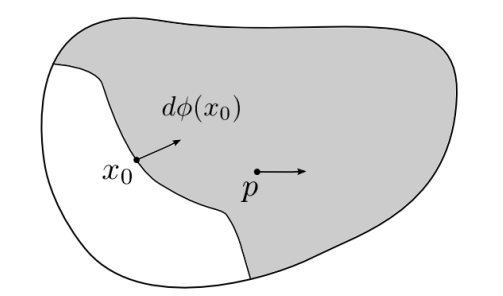
Let X๐‘‹X be a complex analytic manifold and consider a complex of coherent sheaves โ„ฑโˆ™.superscriptโ„ฑโˆ™\mathcal{F}^{\bullet}. It is said said to โ€˜propagate in the codirection p=(x0;ฮพ0)โˆˆTโˆ—โ€‹X๐‘subscript๐‘ฅ0subscript๐œ‰0superscript๐‘‡๐‘‹p=(x_{0};\xi_{0})\in T^{*}Xโ€™ if: for all open subsets U๐‘ˆU in X๐‘‹X with x0โˆˆโˆ‚Usubscript๐‘ฅ0๐‘ˆx_{0}\in\partial U where โˆ‚U๐‘ˆ\partial U is smooth in a neighbourhood of x0subscript๐‘ฅ0x_{0} and ฮพ0subscript๐œ‰0\xi_{0} is the exterior normal vector to U๐‘ˆU at x0subscript๐‘ฅ0x_{0}, then any section sโˆˆฮ“โ€‹(U,โ„ฑโˆ™)๐‘ ฮ“๐‘ˆsuperscriptโ„ฑโˆ™s\in\Gamma(U,\mathcal{F}^{\bullet}) extends through x0subscript๐‘ฅ0x_{0} i.e. extends to larger opens UโˆชV๐‘ˆ๐‘‰U\cup V where V๐‘‰V is a neighbourhood of x0.subscript๐‘ฅ0x_{0}.

Definition 2.1.

A complex of coherent sheaves โ„ฑโˆ™superscriptโ„ฑโˆ™\mathcal{F}^{\bullet} on a complex analytic manifolds X๐‘‹X propagates at x0โˆˆXsubscript๐‘ฅ0๐‘‹x_{0}\in X in the direction p๐‘p (see the helpful Figure 1) if for all C1superscript๐ถ1C^{1}-functions ฯ†๐œ‘\varphi with ฯ†โ€‹(x0)=0๐œ‘subscript๐‘ฅ00\varphi(x_{0})=0 and dโ€‹ฯ†โ€‹(x0)=ฮพ0๐‘‘๐œ‘subscript๐‘ฅ0subscript๐œ‰0d\varphi(x_{0})=\xi_{0} the natural map ฯjโ€‹(x0):limโ†’Uโˆ‹x0โ€‹Hjโ€‹(U;โ„ฑ)โ†’limโ†’Uโˆ‹x0โ€‹Hjโ€‹(Uโˆฉ{ฯ†<0};โ„ฑ):subscript๐œŒ๐‘—subscript๐‘ฅ0โ†’subscript๐‘ฅ0๐‘ˆinjective-limitsuperscript๐ป๐‘—๐‘ˆโ„ฑsubscript๐‘ฅ0๐‘ˆinjective-limitsuperscript๐ป๐‘—๐‘ˆ๐œ‘0โ„ฑ\rho_{j}(x_{0}):\underset{U\ni x_{0}}{\varinjlim}\hskip 1.42262ptH^{j}(U;\mathcal{F})\rightarrow\underset{U\ni x_{0}}{\varinjlim}\hskip 1.42262ptH^{j}\big{(}U\cap\{\varphi<0\};\mathcal{F}\big{)} is an isomorphism for all j.๐‘—j.

Definition 2.1 tells us that for a given covector at a point, understood as a hyperplane in the tangent space, we are studying whether a sheaf behaves locally constantly moving off this hypersurface, in the conormal direction. As we will see in Subsect.2.1, this interpretation generalizes the Cauchy-Kovalevskaya theorem for PDEs (see Theorem 2.7 below).

Figure 1. Propagation in codirection p๐‘p. Graphic borrowed from P. Schapira [Sch16].
Refer to caption

Propagation isomorphisms ฯjโ€‹(x0)subscript๐œŒ๐‘—subscript๐‘ฅ0\rho_{j}(x_{0}) are seen to be equivalent to

(2.1) (Rโ€‹ฮ“{ฯ†โ‰ฅ0}โ€‹(โ„ฑโˆ™))x0=0(Propagation atย โ€‹x0โˆˆX).subscript๐‘…subscriptฮ“๐œ‘0superscriptโ„ฑโˆ™subscript๐‘ฅ00Propagation atย subscript๐‘ฅ0๐‘‹\big{(}R\Gamma_{\{\varphi\geq 0\}}(\mathcal{F}^{\bullet})\big{)}_{x_{0}}=0\hskip 14.22636pt\big{(}\text{Propagation at }x_{0}\in X\big{)}.

Microsupport collects all places where there is no propagation i.e. the set of codirections of non-propagation, corresponding to points p=(x0;ฮพ0)โˆˆTโˆ—โ€‹X,๐‘subscript๐‘ฅ0subscript๐œ‰0superscript๐‘‡๐‘‹p=(x_{0};\xi_{0})\in T^{*}X, where ฯjโ€‹(x0)subscript๐œŒ๐‘—subscript๐‘ฅ0\rho_{j}(x_{0}) is not an isomorphism. Define the set of propagation of โ„ฑโˆ™,superscriptโ„ฑโˆ™\mathcal{F}^{\bullet},

P(โ„ฑโˆ™):={(x;ฮพ)โˆˆTโˆ—X|\displaystyle P(\mathcal{F}^{\bullet}):=\{(x;\xi)\in T^{*}X| โˆ€for-all\displaystyle\forall open neighbourhoodsย โ€‹Uโ€‹ย ofย โ€‹xโ€‹ย andย โ€‹ฯ†โˆˆCโˆžโ€‹(U)open neighbourhoodsย ๐‘ˆย ofย ๐‘ฅย andย ๐œ‘superscript๐ถ๐‘ˆ\displaystyle\text{open neighbourhoods }U\text{ of }x\text{ and }\varphi\in C^{\infty}(U)
with ฯ†(x)=0,dฯ†(x)=ฮพ,ย one hasย (2.1)}.\displaystyle\varphi(x)=0,d\varphi(x)=\xi,\text{ one has }(\ref{eqn: ShvProp@x})\}.
Definition 2.2.

The microsupport of โ„ฑโˆ™superscriptโ„ฑโˆ™\mathcal{F}^{\bullet} is the closure of the set of codirections of non-propagation, ฮผโ€‹sโ€‹uโ€‹pโ€‹pโ€‹(โ„ฑโˆ™):=Tโˆ—โ€‹X\Pโ€‹(โ„ฑโˆ™)ยฏ.assign๐œ‡๐‘ ๐‘ข๐‘๐‘superscriptโ„ฑโˆ™ยฏ\superscript๐‘‡๐‘‹๐‘ƒsuperscriptโ„ฑโˆ™\mu supp(\mathcal{F}^{\bullet}):=\overline{T^{*}X\hskip 2.84526pt\backslash\hskip 2.84526ptP(\mathcal{F}^{\bullet})}.

The microsupport (2.2) is a coisotropic closed โ„‚ร—superscriptโ„‚\mathbb{C}^{\times}-conic subset of Tโˆ—โ€‹Msuperscript๐‘‡๐‘€T^{*}M such that TMโˆ—โ€‹Mโˆฉฮผโ€‹sโ€‹uโ€‹pโ€‹pโ€‹(F)=ฯ€Mโ€‹(ฮผโ€‹sโ€‹uโ€‹pโ€‹pโ€‹(F))=sโ€‹uโ€‹pโ€‹pโ€‹(F)superscriptsubscript๐‘‡๐‘€๐‘€๐œ‡๐‘ ๐‘ข๐‘๐‘๐นsubscript๐œ‹๐‘€๐œ‡๐‘ ๐‘ข๐‘๐‘๐น๐‘ ๐‘ข๐‘๐‘๐นT_{M}^{*}M\cap\mu supp(F)=\pi_{M}\big{(}\mu supp(F)\big{)}=supp(F), and ฮผโ€‹sโ€‹uโ€‹pโ€‹pโ€‹(Fโ€‹[i])=ฮผโ€‹sโ€‹uโ€‹pโ€‹pโ€‹(F)๐œ‡๐‘ ๐‘ข๐‘๐‘๐นdelimited-[]๐‘–๐œ‡๐‘ ๐‘ข๐‘๐‘๐น\mu supp(F[i])=\mu supp(F) for iโˆˆโ„ค.๐‘–โ„คi\in\mathbb{Z}. Moreover, it satisfies the triangular inequality: for a triangle F1โ†’F2โ†’F3โ†’+1โ†’subscript๐น1subscript๐น2โ†’subscript๐น31โ†’absentF_{1}\rightarrow F_{2}\rightarrow F_{3}\xrightarrow{+1} in Dbโ€‹(๐คM)superscriptDbsubscript๐ค๐‘€\mathrm{D}^{\mathrm{b}}(\mathbf{k}_{M}) then ฮผโ€‹sโ€‹uโ€‹pโ€‹pโ€‹(Fi)โŠ‚ฮผโ€‹sโ€‹uโ€‹pโ€‹pโ€‹(Fj)โˆชฮผโ€‹sโ€‹uโ€‹pโ€‹pโ€‹(Fk)๐œ‡๐‘ ๐‘ข๐‘๐‘subscript๐น๐‘–๐œ‡๐‘ ๐‘ข๐‘๐‘subscript๐น๐‘—๐œ‡๐‘ ๐‘ข๐‘๐‘subscript๐น๐‘˜\mu supp(F_{i})\subset\mu supp(F_{j})\cup\mu supp(F_{k}) for i,j,kโˆˆ{1,2,3}๐‘–๐‘—๐‘˜123i,j,k\in\{1,2,3\} with jโ‰ k.๐‘—๐‘˜j\neq k.

Example 2.3.

Let UโŠ‚M๐‘ˆ๐‘€U\subset M be an open subset with smooth boundary and consider: Zฮป:={(x;ฮปโ€‹dโ€‹fโ€‹(x))|fโ€‹(x)=0,ฮปโ‰ค0},assignsubscript๐‘๐œ†conditional-set๐‘ฅ๐œ†๐‘‘๐‘“๐‘ฅformulae-sequence๐‘“๐‘ฅ0๐œ†0Z_{\lambda}:=\{(x;\lambda df(x))|f(x)=0,\lambda\leq 0\}, such that U={f>0}๐‘ˆ๐‘“0U=\{f>0\} and dโ€‹fโ‰ 0๐‘‘๐‘“0df\neq 0 on โˆ‚U๐‘ˆ\partial U. Then ฮผโ€‹sโ€‹uโ€‹pโ€‹pโ€‹(๐คU)=(Uร—MTMโˆ—โ€‹M)โˆชZฮป,๐œ‡๐‘ ๐‘ข๐‘๐‘subscript๐ค๐‘ˆsubscript๐‘€๐‘ˆsuperscriptsubscript๐‘‡๐‘€๐‘€subscript๐‘๐œ†\mu supp(\mathbf{k}_{U})=(U\times_{M}T_{M}^{*}M)\cup Z_{\lambda}, while ฮผโ€‹sโ€‹uโ€‹pโ€‹pโ€‹(๐คUยฏ)=(Uร—MTMโˆ—โ€‹M)โˆชZฮปa,๐œ‡๐‘ ๐‘ข๐‘๐‘subscript๐คยฏ๐‘ˆsubscript๐‘€๐‘ˆsuperscriptsubscript๐‘‡๐‘€๐‘€superscriptsubscript๐‘๐œ†๐‘Ž\mu supp(\mathbf{k}_{\underline{U}})=(U\times_{M}T_{M}^{*}M)\cup Z_{\lambda}^{a}, with Zฮปasuperscriptsubscript๐‘๐œ†๐‘ŽZ_{\lambda}^{a} its image by the antipodal map. This follows from Rโ€‹ฮ“{x|fโ€‹(x)โ‰ฅ0}โ€‹(๐คU)โ‰ƒ๐คUsimilar-to-or-equals๐‘…subscriptฮ“conditional-set๐‘ฅ๐‘“๐‘ฅ0subscript๐ค๐‘ˆsubscript๐ค๐‘ˆR\Gamma_{\{x|f(x)\geq 0\}}(\mathbf{k}_{U})\simeq\mathbf{k}_{U}, (and similarly for ๐คUยฏsubscript๐คยฏ๐‘ˆ\mathbf{k}_{\overline{U}}).

Intuitively, Example 2.3 states that directions of propagation of a constant sheaf on an open (resp. closed) subset with smooth boundary point in the outward (resp. inward) normal directions.

Proposition 2.4.

Fix x0โˆˆM.subscript๐‘ฅ0๐‘€x_{0}\in M. Then ฮพโˆˆPx0โ€‹(โ„ฑโˆ™)๐œ‰subscript๐‘ƒsubscript๐‘ฅ0superscriptโ„ฑโˆ™\xi\in P_{x_{0}}(\mathcal{F}^{\bullet}) if and only if for every ฯ†โˆˆCโˆžโ€‹(U,โ„‚)๐œ‘superscript๐ถ๐‘ˆโ„‚\varphi\in C^{\infty}(U,\mathbb{C}) for an open neighbourhood U๐‘ˆU of x0subscript๐‘ฅ0x_{0} such that ฯ†โ€‹(x0)=0๐œ‘subscript๐‘ฅ00\varphi(x_{0})=0 and dโ€‹ฯ†โ€‹(x0)=ฮพ๐‘‘๐œ‘subscript๐‘ฅ0๐œ‰d\varphi(x_{0})=\xi, the morphism โ„ฑx0โˆ™โ†’(Rโ€‹ฮ“{ฯ†<0}โ€‹(โ„ฑโˆ™))x0,โ†’superscriptsubscriptโ„ฑsubscript๐‘ฅ0โˆ™subscript๐‘…subscriptฮ“๐œ‘0superscriptโ„ฑโˆ™subscript๐‘ฅ0\mathcal{F}_{x_{0}}^{\bullet}\rightarrow\big{(}R\Gamma_{\{\varphi<0\}}(\mathcal{F}^{\bullet})\big{)}_{x_{0}}, induced by the inclusion (iV:Vโˆฉ{ฯ†<0}โ†ชV)x0โˆˆV\big{(}i_{V}:V\cap\{\varphi<0\}\hookrightarrow V\big{)}_{x_{0}\in V} is an isomorphism.

Proof.

Apply the stalks functor to Rโ€‹ฮ“{ฯ†โ‰ฅ0}โ€‹(F)โ†’Rโ€‹ฮ“Uโ€‹(F)โ†’Rโ€‹ฮ“{ฯ†<0}โ€‹(F)โ†’+1.โ†’๐‘…subscriptฮ“๐œ‘0๐น๐‘…subscriptฮ“๐‘ˆ๐นโ†’๐‘…subscriptฮ“๐œ‘0๐น1โ†’absentR\Gamma_{\{\varphi\geq 0\}}(F)\rightarrow R\Gamma_{U}(F)\rightarrow R\Gamma_{\{\varphi<0\}}(F)\xrightarrow{+1}. โˆŽ

Proposition 2.4 characterizes when a point belongs to Pโ€‹(โ„ฑโˆ™).๐‘ƒsuperscriptโ„ฑโˆ™P(\mathcal{F}^{\bullet}).

Proposition 2.5.

Let FโˆˆDbโ€‹(๐คM),GโˆˆDbโ€‹(๐คN).formulae-sequence๐นsuperscriptDbsubscript๐ค๐‘€๐บsuperscriptD๐‘subscript๐ค๐‘F\in\mathrm{D}^{\mathrm{b}}(\mathbf{k}_{M}),G\in\mathrm{D}^{b}(\mathbf{k}_{N}). Then ฮผโ€‹sโ€‹uโ€‹pโ€‹pโ€‹(FโŠ LG)โŠ‚ฮผโ€‹sโ€‹uโ€‹pโ€‹pโ€‹(F)ร—ฮผโ€‹sโ€‹uโ€‹pโ€‹pโ€‹(G).๐œ‡๐‘ ๐‘ข๐‘๐‘superscriptโŠ ๐ฟ๐น๐บ๐œ‡๐‘ ๐‘ข๐‘๐‘๐น๐œ‡๐‘ ๐‘ข๐‘๐‘๐บ\mu supp(F\boxtimes^{L}G)\subset\mu supp(F)\times\mu supp(G). If f:Nโ†’M:๐‘“โ†’๐‘๐‘€f:N\rightarrow M is proper on sโ€‹uโ€‹pโ€‹pโ€‹(F),๐‘ ๐‘ข๐‘๐‘๐นsupp(F), then Rโ€‹f!โ€‹Fโ†’โ‰ƒRโ€‹fโˆ—โ€‹Fsimilar-to-or-equalsโ†’๐‘…subscript๐‘“๐น๐‘…subscript๐‘“๐นRf_{!}F\xrightarrow{\simeq}Rf_{*}F and ฮผโ€‹sโ€‹uโ€‹pโ€‹pโ€‹(Rโ€‹fโˆ—โ€‹F)โŠ‚fฯ€โ€‹fdโˆ’1โ€‹ฮผโ€‹sโ€‹uโ€‹pโ€‹pโ€‹(F).๐œ‡๐‘ ๐‘ข๐‘๐‘๐‘…subscript๐‘“๐นsubscript๐‘“๐œ‹superscriptsubscript๐‘“๐‘‘1๐œ‡๐‘ ๐‘ข๐‘๐‘๐น\mu supp(Rf_{*}F)\subset f_{\pi}f_{d}^{-1}\mu supp(F). Moreover, if f๐‘“f is a closed embedding, ฮผโ€‹sโ€‹uโ€‹pโ€‹pโ€‹(Rโ€‹fโˆ—โ€‹F)=fฯ€โ€‹fdโˆ’1โ€‹ฮผโ€‹sโ€‹uโ€‹pโ€‹pโ€‹(F).๐œ‡๐‘ ๐‘ข๐‘๐‘๐‘…subscript๐‘“๐นsubscript๐‘“๐œ‹superscriptsubscript๐‘“๐‘‘1๐œ‡๐‘ ๐‘ข๐‘๐‘๐น\mu supp(Rf_{*}F)=f_{\pi}f_{d}^{-1}\mu supp(F).

Example 2.6.

Consider a smooth morphism f:Xโ†’Y:๐‘“โ†’๐‘‹๐‘Œf:X\rightarrow Y and a Lagrangian sub-manifold ฮ›โŠ‚Tโˆ—โ€‹Xยฏร—Tโˆ—โ€‹Y.ฮ›ยฏsuperscript๐‘‡๐‘‹superscript๐‘‡๐‘Œ\Lambda\subset\overline{T^{*}X}\times T^{*}Y. For a subset SโŠ‚Tโˆ—โ€‹X๐‘†superscript๐‘‡๐‘‹S\subset T^{*}X define ฮ›โ€‹(S)ฮ›๐‘†\Lambda(S) to be the reduction of Sร—ฮ›๐‘†ฮ›S\times\Lambda by the cositropic submanifold Dร—Tโˆ—โ€‹Y๐ทsuperscript๐‘‡๐‘ŒD\times T^{*}Y, with D๐ทD the diagonal in Tโˆ—โ€‹Xร—Tโˆ—โ€‹Xยฏ.superscript๐‘‡๐‘‹ยฏsuperscript๐‘‡๐‘‹T^{*}X\times\overline{T^{*}X}. Define ฮ›f:={(x,ฮพ,y;p)โˆˆTโˆ—โ€‹Xยฏร—Tโˆ—โ€‹Y|fโ€‹(x)=y,ฮพ=pโˆ˜dโ€‹fโ€‹(x)}.assignsubscriptฮ›๐‘“conditional-set๐‘ฅ๐œ‰๐‘ฆ๐‘ยฏsuperscript๐‘‡๐‘‹superscript๐‘‡๐‘Œformulae-sequence๐‘“๐‘ฅ๐‘ฆ๐œ‰๐‘๐‘‘๐‘“๐‘ฅ\Lambda_{f}:=\{(x,\xi,y;p)\in\overline{T^{*}X}\times T^{*}Y|f(x)=y,\xi=p\circ df(x)\}. For SโŠ‚Tโˆ—โ€‹X,๐‘†superscript๐‘‡๐‘‹S\subset T^{*}X, we have (y;p)โˆˆฮ›fโ€‹(S)๐‘ฆ๐‘subscriptฮ›๐‘“๐‘†(y;p)\in\Lambda_{f}(S) if and only if there exists xโˆˆfโˆ’1โ€‹(y)๐‘ฅsuperscript๐‘“1๐‘ฆx\in f^{-1}(y) such that (x,pโˆ˜dโ€‹fโ€‹(x))โˆˆS.๐‘ฅ๐‘๐‘‘๐‘“๐‘ฅ๐‘†(x,p\circ df(x))\in S. If f๐‘“f moreover proper on sโ€‹uโ€‹pโ€‹pโ€‹(โ„ฑ)๐‘ ๐‘ข๐‘๐‘โ„ฑsupp(\mathcal{F}), then ฮผโ€‹sโ€‹uโ€‹pโ€‹pโ€‹(Rโ€‹fโˆ—โ€‹โ„ฑ)โŠ‚ฮ›fโ€‹(ฮผโ€‹sโ€‹uโ€‹pโ€‹pโ€‹(โ„ฑ)).๐œ‡๐‘ ๐‘ข๐‘๐‘๐‘…subscript๐‘“โ„ฑsubscriptฮ›๐‘“๐œ‡๐‘ ๐‘ข๐‘๐‘โ„ฑ\mu supp(Rf_{*}\mathcal{F})\subset\Lambda_{f}(\mu supp(\mathcal{F})\big{)}.

Example 2.6 shows that if a sheaf โ„ฑโ„ฑ\mathcal{F} propagates at (x,pโˆ˜dโ€‹fโ€‹(x))๐‘ฅ๐‘๐‘‘๐‘“๐‘ฅ\big{(}x,p\circ df(x)\big{)} for each x๐‘ฅx in fโˆ’1โ€‹(y)superscript๐‘“1๐‘ฆf^{-1}(y), then Rโ€‹fโˆ—โ€‹โ„ฑ๐‘…subscript๐‘“โ„ฑRf_{*}\mathcal{F} propagates at (y;p).๐‘ฆ๐‘(y;p).

2.1. Propagation of Solutions

We can now analyze the propagation of solutions by taking โ„ฑโˆ™superscriptโ„ฑโˆ™\mathcal{F}^{\bullet} to be the sheaf Rโ€‹SolX,lโ€‹iโ€‹nโ€‹(โ„ณ)๐‘…subscriptSol๐‘‹๐‘™๐‘–๐‘›โ„ณR\mathrm{Sol}_{X,lin}(\mathcal{M}) of solutions to a coherent ๐’ŸXsubscript๐’Ÿ๐‘‹\mathcal{D}_{X}-module associated to a system of linear PDEs.

Theorem 2.7 ([SK90, Prop. 11.5.4]).

Let โ„ณโ„ณ\mathcal{M} be a coherent โ„ฐXsubscriptโ„ฐ๐‘‹\mathcal{E}_{X}-module and denote the microfunction-valued solution sheaf โ„โ€‹โ„‹โ€‹oโ€‹mโ„ฐXโ€‹(โ„ณ,๐’žM),โ„โ„‹๐‘œsubscript๐‘šsubscriptโ„ฐ๐‘‹โ„ณsubscript๐’ž๐‘€\mathbb{R}\mathcal{H}om_{\mathcal{E}_{X}}(\mathcal{M},\mathcal{C}_{M}), by Rโ€‹Sโ€‹oโ€‹lโ„ฐXโ€‹(โ„ณ).๐‘…๐‘†๐‘œsubscript๐‘™subscriptโ„ฐ๐‘‹โ„ณRSol_{\mathcal{E}_{X}}(\mathcal{M}). Then,

ฮผโ€‹sโ€‹uโ€‹pโ€‹pโ€‹(Rโ€‹Sโ€‹oโ€‹lโ„ฐXโ€‹(โ„ณ))โŠ‚CTMโˆ—โ€‹Xโ€‹(Charโ€‹(โ„ณ))โŠ‚Tโˆ—โ€‹Tโˆ—โ€‹X.๐œ‡๐‘ ๐‘ข๐‘๐‘๐‘…๐‘†๐‘œsubscript๐‘™subscriptโ„ฐ๐‘‹โ„ณsubscript๐ถsuperscriptsubscript๐‘‡๐‘€๐‘‹Charโ„ณsuperscript๐‘‡superscript๐‘‡๐‘‹\mu supp\big{(}RSol_{\mathcal{E}_{X}}(\mathcal{M})\big{)}\subset C_{T_{M}^{*}X}\big{(}\mathrm{Char}(\mathcal{M})\big{)}\subset T^{*}T^{*}X.

In particular sโ€‹uโ€‹pโ€‹pโ€‹(Rโ€‹Sโ€‹oโ€‹lโ„ฐXโ€‹(โ„ณ))โŠ‚Charโ€‹(โ„ณ)โˆฉTMโˆ—โ€‹X๐‘ ๐‘ข๐‘๐‘๐‘…๐‘†๐‘œsubscript๐‘™subscriptโ„ฐ๐‘‹โ„ณCharโ„ณsuperscriptsubscript๐‘‡๐‘€๐‘‹supp\big{(}RSol_{\mathcal{E}_{X}}(\mathcal{M})\big{)}\subset\mathrm{Char}(\mathcal{M})\cap T_{M}^{*}X and if โ„ณโ„ณ\mathcal{M} is a coherent ๐’ŸXsubscript๐’Ÿ๐‘‹\mathcal{D}_{X}-module, then ฮผsupp((RSolX(โ„ณ,๐’ชX))=Char(โ„ณ).\mu supp\big{(}(RSol_{X}(\mathcal{M},\mathcal{O}_{X})\big{)}=Char(\mathcal{M}).

Recall the relation between microlocalizations and characteristic varieties. For a coherent ๐’ŸXsubscript๐’Ÿ๐‘‹\mathcal{D}_{X}-module โ„ณโ„ณ\mathcal{M} its microlocalization is ฮผโ€‹โ„ณ:=โ„ฐXโŠ—ฯ€โˆ’1โ€‹๐’ŸXฯ€โˆ’1โ€‹โ„ณ,assign๐œ‡โ„ณsubscripttensor-productsuperscript๐œ‹1subscript๐’Ÿ๐‘‹subscriptโ„ฐ๐‘‹superscript๐œ‹1โ„ณ\mu\mathcal{M}:=\mathcal{E}_{X}\otimes_{\pi^{-1}\mathcal{D}_{X}}\pi^{-1}\mathcal{M}, for ฯ€:Tโˆ—โ€‹Xโ†’X:๐œ‹โ†’superscript๐‘‡๐‘‹๐‘‹\pi:T^{*}X\rightarrow X, which is coherent as an โ„ฐXsubscriptโ„ฐ๐‘‹\mathcal{E}_{X}-module. The characteristic variety of โ„ณโ„ณ\mathcal{M} is the support of its microlocalization

Cโ€‹hโ€‹aโ€‹rโ€‹(โ„ณ):=sโ€‹uโ€‹pโ€‹pโ€‹(ฮผโ€‹โ„ณ).assign๐ถโ„Ž๐‘Ž๐‘Ÿโ„ณ๐‘ ๐‘ข๐‘๐‘๐œ‡โ„ณChar(\mathcal{M}):=supp\big{(}\mu\mathcal{M}\big{)}.
Example 2.8.

Suppose that P=Pโ€‹(x,โˆ‚x)โˆˆ๐’ŸXโ‰คmโŠ‚๐’ŸX๐‘ƒ๐‘ƒ๐‘ฅsubscript๐‘ฅsuperscriptsubscript๐’Ÿ๐‘‹absent๐‘šsubscript๐’Ÿ๐‘‹P=P(x,\partial_{x})\in\mathcal{D}_{X}^{\leq m}\subset\mathcal{D}_{X} is a differential operator of order โ‰คm.absent๐‘š\leq m. By Theorem 2.7, P๐‘ƒP defines an isomorphism of the sheaf ๐’žMsubscript๐’ž๐‘€\mathcal{C}_{M} on TMโˆ—โ€‹X\{ฯƒmโ€‹(P)โˆ’1โ€‹(0)}\superscriptsubscript๐‘‡๐‘€๐‘‹subscript๐œŽ๐‘šsuperscript๐‘ƒ10T_{M}^{*}X\backslash\big{\{}\sigma_{m}(P)^{-1}(0)\big{\}} and if u๐‘ขu is a hyperfunction solution, its support is contained in the union of the support of Pโ€‹u๐‘ƒ๐‘ขPu and {ฯƒmโ€‹(P)โˆ’1โ€‹(0)}.subscript๐œŽ๐‘šsuperscript๐‘ƒ10\big{\{}\sigma_{m}(P)^{-1}(0)\big{\}}.

The abstract propagation result for linear systems in Theorem 2.7 is related to local-constancy of the sheaf of solutions and the condition for propagation (2.1) as follows.

Proposition 2.9 ([SK90, Proposition 11.5.6]).

Let U๐‘ˆU be an open subset of Tโˆ—โ€‹Xsuperscript๐‘‡๐‘‹T^{*}X and suppose gโˆˆ๐’ชโ€‹(U)๐‘”๐’ช๐‘ˆg\in\mathcal{O}(U) is such that Iโ€‹mโ€‹(g)๐ผ๐‘š๐‘”Im(g) vanishes on TMโˆ—โ€‹X.superscriptsubscript๐‘‡๐‘€๐‘‹T_{M}^{*}X. Then for all pโˆˆUโˆฉTMโˆ—โ€‹X๐‘๐‘ˆsuperscriptsubscript๐‘‡๐‘€๐‘‹p\in U\cap T_{M}^{*}X the bicharacteristic curve ฮฒpsubscript๐›ฝ๐‘\beta_{p} passing through p๐‘p of the involutive submanifold {Iโ€‹mโ€‹(g)=0}๐ผ๐‘š๐‘”0\{Im(g)=0\} of (Tโˆ—X)โ„(T^{*}X){{}^{\mathbb{R}}} is contained in a neighbourhood of p๐‘p in TMโˆ—โ€‹X.superscriptsubscript๐‘‡๐‘€๐‘‹T_{M}^{*}X. Suppose โ„ณโˆˆ๐–ข๐—ˆ๐—โ€‹(๐’ŸX)โ„ณ๐–ข๐—ˆ๐—subscript๐’Ÿ๐‘‹\mathcal{M}\in\mathsf{Coh}(\mathcal{D}_{X}) with Iโ€‹mโ€‹(g)|TMโˆ—โ€‹XโˆฉU=0.evaluated-at๐ผ๐‘š๐‘”superscriptsubscript๐‘‡๐‘€๐‘‹๐‘ˆ0Im(g)\big{|}_{T_{M}^{*}X\cap U}=0. Assume that Cโ€‹hโ€‹aโ€‹rโ€‹(โ„ณ)โˆฉUโŠ‚{g=0}.๐ถโ„Ž๐‘Ž๐‘Ÿโ„ณ๐‘ˆ๐‘”0Char(\mathcal{M})\cap U\subset\{g=0\}. Then for all bicharacteristics ฮฒ๐›ฝ\beta of the manifold {Iโ€‹mโ€‹(g)=0}๐ผ๐‘š๐‘”0\{Im(g)=0\}, the sheaves ๐–ฒ๐—ˆ๐—…X,lโ€‹iโ€‹njโ€‹(โ„ณ,๐’žM)|ฮฒ=โ„ฐโ€‹๐—‘๐—๐’ŸXjโ€‹(โ„ณ,๐’žM)|ฮฒ,evaluated-atsuperscriptsubscript๐–ฒ๐—ˆ๐—…๐‘‹๐‘™๐‘–๐‘›๐‘—โ„ณsubscript๐’ž๐‘€๐›ฝevaluated-atโ„ฐsuperscriptsubscript๐—‘๐—subscript๐’Ÿ๐‘‹๐‘—โ„ณsubscript๐’ž๐‘€๐›ฝ\mathsf{Sol}_{X,lin}^{j}(\mathcal{M},\mathcal{C}_{M})\big{|}_{\beta}=\mathcal{E}\mathsf{xt}_{\mathcal{D}_{X}}^{j}\big{(}\mathcal{M},\mathcal{C}_{M}\big{)}\big{|}_{\beta}, are locally constant, (jโˆˆโ„•๐‘—โ„•j\in\mathbb{N}).

In other words, for p0=(x0,ฮพ0)subscript๐‘0subscript๐‘ฅ0subscript๐œ‰0p_{0}=(x_{0},\xi_{0}) and ฮฒp0subscript๐›ฝsubscript๐‘0\beta_{p_{0}} as in Proposition 2.9, we have

Rโ€‹ฮ“{ฮฒp0}โ€‹(๐–ฒ๐—ˆ๐—…X,lโ€‹iโ€‹njโ€‹(โ„ณ,๐’žM)|ฮฒ)x0โ‰ƒ0,similar-to-or-equals๐‘…subscriptฮ“subscript๐›ฝsubscript๐‘0subscriptevaluated-atsuperscriptsubscript๐–ฒ๐—ˆ๐—…๐‘‹๐‘™๐‘–๐‘›๐‘—โ„ณsubscript๐’ž๐‘€๐›ฝsubscript๐‘ฅ00R\Gamma_{\{\beta_{p_{0}}\}}\big{(}\mathsf{Sol}_{X,lin}^{j}(\mathcal{M},\mathcal{C}_{M})\big{|}_{\beta}\big{)}_{x_{0}}\simeq 0,

since ฮผsupp(๐–ฒ๐—ˆ๐—…โ„ฐX(โ„ณ))โŠ‚CTMโˆ—โ€‹X({gโˆ’1(0)})={ฮธโˆˆTโˆ—TMโˆ—X|<ฮธ,Hg>=0}.\mu supp\big{(}\mathsf{Sol}_{\mathcal{E}_{X}}(\mathcal{M})\big{)}\subset C_{T_{M}^{*}X}\big{(}\{g^{-1}(0)\}\big{)}=\big{\{}\theta\in T^{*}T_{M}^{*}X|<\theta,H_{g}>=0\big{\}}.

2.1.1.

When considering elliptic or hyperbolic operators one can modify the definition of the characteristic varieties to also encode the directions of (non)-propagation for their solutions. Then, hyperbolicity appears as a geometric condition of the characteristic variety.

Let M๐‘€M be a real manifold with complexification X.๐‘‹X. A coherent ๐’ŸXsubscript๐’Ÿ๐‘‹\mathcal{D}_{X}-module โ„ณโ„ณ\mathcal{M} is elliptic if TฬŠMโˆ—โ€‹XโˆฉCโ€‹hโ€‹aโ€‹rโ€‹(โ„ณ)=โˆ…superscriptsubscriptฬŠ๐‘‡๐‘€๐‘‹๐ถโ„Ž๐‘Ž๐‘Ÿโ„ณ\mathring{T}_{M}^{*}X\cap Char(\mathcal{M})=\emptyset, or equivalently,

TMโˆ—โ€‹XโˆฉCโ€‹hโ€‹aโ€‹rโ€‹(โ„ณ)โŠ‚TXโˆ—โ€‹X,superscriptsubscript๐‘‡๐‘€๐‘‹๐ถโ„Ž๐‘Ž๐‘Ÿโ„ณsuperscriptsubscript๐‘‡๐‘‹๐‘‹T_{M}^{*}X\cap Char(\mathcal{M})\subset T_{X}^{*}X,

Theorem 2.7 implies elliptic regularity; the inclusion of analytic solutions in hyperfunction solutions

Rโ€‹๐–ฒ๐—ˆ๐—…Xโ€‹(โ„ณ,๐’œM)โ†’โ‰ƒRโ€‹๐–ฒ๐—ˆ๐—…Xโ€‹(โ„ณ,โ„ฌM),similar-to-or-equalsโ†’๐‘…subscript๐–ฒ๐—ˆ๐—…๐‘‹โ„ณsubscript๐’œ๐‘€๐‘…subscript๐–ฒ๐—ˆ๐—…๐‘‹โ„ณsubscriptโ„ฌ๐‘€R\mathsf{Sol}_{X}(\mathcal{M},\mathcal{A}_{M})\xrightarrow{\simeq}R\mathsf{Sol}_{X}(\mathcal{M},\mathcal{B}_{M}),

induced from sequence (1.7) is an isomorphism.

Remark 2.10.

Important results are known for hyperbolic systems and the propagation of their solution sheaves. For example, the propagation of hyperfunction and distribution solutions to hyperbolic systems on Lorentzian space-times (e.g. time-oriented Lorentzian manifolds) was studied in [JS16].

One says that ฮธโˆˆTTMโˆ—โ€‹Xโ€‹Tโˆ—โ€‹X๐œƒsubscript๐‘‡superscriptsubscript๐‘‡๐‘€๐‘‹superscript๐‘‡๐‘‹\theta\in T_{T_{M}^{*}X}T^{*}X is microhyperbolic for a ๐’ŸXsubscript๐’Ÿ๐‘‹\mathcal{D}_{X}-module โ„ณโ„ณ\mathcal{M} if ฮธโˆ‰CTMโˆ—โ€‹Xโ€‹(Cโ€‹hโ€‹aโ€‹rโ€‹(โ„ณ)).๐œƒsubscript๐ถsuperscriptsubscript๐‘‡๐‘€๐‘‹๐ถโ„Ž๐‘Ž๐‘Ÿโ„ณ\theta\notin C_{T_{M}^{*}X}\big{(}Char(\mathcal{M})\big{)}. Under ฮธโˆˆTโˆ—โ€‹Mโ†ชTTMโˆ—โ€‹Xโ€‹Tโˆ—โ€‹X๐œƒsuperscript๐‘‡๐‘€โ†ชsubscript๐‘‡superscriptsubscript๐‘‡๐‘€๐‘‹superscript๐‘‡๐‘‹\theta\in T^{*}M\hookrightarrow T_{T_{M}^{*}X}T^{*}X, one says ฮธ๐œƒ\theta is hyperbolic for โ„ณ.โ„ณ\mathcal{M}.

If ฮธ๐œƒ\theta is microhyperbolic (resp. hyperbolic) this implies that ฮธโˆ‰ฮผโ€‹sโ€‹uโ€‹pโ€‹pโ€‹(Rโ€‹๐–ฒ๐—ˆ๐—…X,lโ€‹iโ€‹nโ€‹(โ„ณ,๐’žM))๐œƒ๐œ‡๐‘ ๐‘ข๐‘๐‘๐‘…subscript๐–ฒ๐—ˆ๐—…๐‘‹๐‘™๐‘–๐‘›โ„ณsubscript๐’ž๐‘€\theta\notin\mu supp\big{(}R\mathsf{Sol}_{X,lin}(\mathcal{M},\mathcal{C}_{M})\big{)} (resp. ฮธโˆ‰ฮผโ€‹sโ€‹uโ€‹pโ€‹pโ€‹(Rโ€‹๐–ฒ๐—ˆ๐—…X,lโ€‹iโ€‹nโ€‹(โ„ณ,โ„ฌ))๐œƒ๐œ‡๐‘ ๐‘ข๐‘๐‘๐‘…subscript๐–ฒ๐—ˆ๐—…๐‘‹๐‘™๐‘–๐‘›โ„ณโ„ฌ\theta\notin\mu supp\big{(}R\mathsf{Sol}_{X,lin}(\mathcal{M},\mathcal{B})\big{)}).

It is equivalently formulated via the hyperbolic characteristic variety of โ„ณโ„ณ\mathcal{M} along M๐‘€M,

(2.2) Cโ€‹hโ€‹aโ€‹rMhโ€‹yโ€‹pโ€‹(โ„ณ):=Tโˆ—โ€‹MโˆฉCTMโˆ—โ€‹Xโ€‹(Cโ€‹hโ€‹aโ€‹rโ€‹(โ„ณ)).assign๐ถโ„Ž๐‘Žsuperscriptsubscript๐‘Ÿ๐‘€โ„Ž๐‘ฆ๐‘โ„ณsuperscript๐‘‡๐‘€subscript๐ถsuperscriptsubscript๐‘‡๐‘€๐‘‹๐ถโ„Ž๐‘Ž๐‘Ÿโ„ณChar_{M}^{hyp}(\mathcal{M}):=T^{*}M\cap C_{T_{M}^{*}X}\big{(}Char(\mathcal{M})\big{)}.

Clearly ฮธโˆˆTโˆ—โ€‹M๐œƒsuperscript๐‘‡๐‘€\theta\in T^{*}M is hyperbolic for โ„ณโ„ณ\mathcal{M} when ฮธโˆ‰Cโ€‹hโ€‹aโ€‹rMhโ€‹yโ€‹pโ€‹(โ„ณ).๐œƒ๐ถโ„Ž๐‘Žsuperscriptsubscript๐‘Ÿ๐‘€โ„Ž๐‘ฆ๐‘โ„ณ\theta\notin Char_{M}^{hyp}(\mathcal{M}).

Example 2.11.

If z=x+iโ€‹yโˆˆX๐‘ง๐‘ฅ๐‘–๐‘ฆ๐‘‹z=x+iy\in X so that M={zโˆˆX|y=0},๐‘€conditional-set๐‘ง๐‘‹๐‘ฆ0M=\{z\in X|y=0\}, and ฮถ=ฮพ+iโ€‹ฮทโˆˆTโˆ—โ€‹X๐œ๐œ‰๐‘–๐œ‚superscript๐‘‡๐‘‹\zeta=\xi+i\eta\in T^{*}X we get TMโˆ—โ€‹X={y=ฮพ=0}.superscriptsubscript๐‘‡๐‘€๐‘‹๐‘ฆ๐œ‰0T_{M}^{*}X=\{y=\xi=0\}. A direction p0=(x0;ฮธ0)โˆˆTโˆ—โ€‹Msubscript๐‘0subscript๐‘ฅ0subscript๐œƒ0superscript๐‘‡๐‘€p_{0}=(x_{0};\theta_{0})\in T^{*}M with ฮธ0โ‰ 0subscript๐œƒ00\theta_{0}\neq 0 is hyperbolic if and only if there exist an open neighbourhood U๐‘ˆU of x0subscript๐‘ฅ0x_{0} in M๐‘€M and open conic neighbourhood ฮณ๐›พ\gamma of ฮธ0โˆˆโ„nsubscript๐œƒ0superscriptโ„๐‘›\theta_{0}\in\mathbb{R}^{n} such that ฯƒโ€‹(P)โ€‹(x;ฮธ+iโ€‹ฮท)โ‰ 0,๐œŽ๐‘ƒ๐‘ฅ๐œƒ๐‘–๐œ‚0\sigma(P)(x;\theta+i\eta)\neq 0, for all ฮทโˆˆโ„n,xโˆˆU,ฮธโˆˆฮณ.formulae-sequence๐œ‚superscriptโ„๐‘›formulae-sequence๐‘ฅ๐‘ˆ๐œƒ๐›พ\eta\in\mathbb{R}^{n},x\in U,\theta\in\gamma.

Remark 2.12.

A submanifold NโŠ‚M๐‘๐‘€N\subset M is hyperbolic for โ„ณโ„ณ\mathcal{M} if TNโˆ—โ€‹MโˆฉCโ€‹hโ€‹aโ€‹rMhโ€‹yโ€‹pโ€‹(โ„ณ)โŠ‚TMโˆ—โ€‹Msuperscriptsubscript๐‘‡๐‘๐‘€๐ถโ„Ž๐‘Žsuperscriptsubscript๐‘Ÿ๐‘€โ„Ž๐‘ฆ๐‘โ„ณsuperscriptsubscript๐‘‡๐‘€๐‘€T_{N}^{*}M\cap Char_{M}^{hyp}(\mathcal{M})\subset T_{M}^{*}M. Obviously, any nonzero covector of TNโˆ—โ€‹Msuperscriptsubscript๐‘‡๐‘๐‘€T_{N}^{*}M is hyperbolic for โ„ณ.โ„ณ\mathcal{M}. Similarly, a real sub-manifold LโŠ‚X๐ฟ๐‘‹L\subset X is elliptic for โ„ณโ„ณ\mathcal{M} if Cโ€‹hโ€‹aโ€‹rโ€‹(โ„ณ)โˆฉTLโˆ—โ€‹XโŠ‚TXโˆ—โ€‹X.๐ถโ„Ž๐‘Ž๐‘Ÿโ„ณsuperscriptsubscript๐‘‡๐ฟ๐‘‹superscriptsubscript๐‘‡๐‘‹๐‘‹Char(\mathcal{M})\cap T_{L}^{*}X\subset T_{X}^{*}X.

By Example 2.11 and Remark 2.12 we can see clearly what geometric hyperbolicity means.

Example 2.13.

Let NโŠ‚M๐‘๐‘€N\subset M be a real submanifold with complexification YโŠ‚X๐‘Œ๐‘‹Y\subset X and โ„ณ=๐’ŸX/๐’ŸXโ‹…Pโ„ณโ‹…subscript๐’Ÿ๐‘‹subscript๐’Ÿ๐‘‹๐‘ƒ\mathcal{M}=\mathcal{D}_{X}/\mathcal{D}_{X}\cdot P a coherent ๐’ŸXsubscript๐’Ÿ๐‘‹\mathcal{D}_{X}-module determined by P๐‘ƒP of order โ‰คk.absent๐‘˜\leq k. Assume (x)=(x1,xโ€ฒ)โˆˆM๐‘ฅsubscript๐‘ฅ1superscript๐‘ฅโ€ฒ๐‘€(x)=(x_{1},x^{\prime})\in M such that N={x1=0}๐‘subscript๐‘ฅ10N=\{x_{1}=0\} and suppose that Cโ€‹hโ€‹aโ€‹rโ€‹(โ„ณ)โˆฉTฬŠโˆ—โ€‹XโˆฉTฬŠMโˆ—โ€‹X๐ถโ„Ž๐‘Ž๐‘Ÿโ„ณsuperscriptฬŠ๐‘‡๐‘‹superscriptsubscriptฬŠ๐‘‡๐‘€๐‘‹Char(\mathcal{M})\cap\mathring{T}^{*}X\cap\mathring{T}_{M}^{*}X is a regular involutive submanifold of TฬŠMโˆ—โ€‹XsuperscriptsubscriptฬŠ๐‘‡๐‘€๐‘‹\mathring{T}_{M}^{*}X and N๐‘N is hyperbolic for โ„ณโ„ณ\mathcal{M}. These assumptions translate to ฯƒโ€‹(P)๐œŽ๐‘ƒ\sigma(P) being a hyperbolic polynomial with respect to N๐‘N with real-constant multiplicities. In other words, ฯƒโ€‹(P)โ€‹(x;ฯ„,ฮทโ€ฒ)๐œŽ๐‘ƒ๐‘ฅ๐œsuperscript๐œ‚โ€ฒ\sigma(P)(x;\tau,\eta^{\prime}) has k๐‘˜k real roots ฯ„๐œ\tau with constant multiplicites where x,ฮทโ€ฒ๐‘ฅsuperscript๐œ‚โ€ฒx,\eta^{\prime} are real.

Hyperfunction, as well as real-analytic solutions of a linear system โ„ณโ„ณ\mathcal{M} propagate in the hyperbolic directions.

Proposition 2.14 ([SK90]).

Suppose that Pโˆˆ๐’ŸX๐‘ƒsubscript๐’Ÿ๐‘‹P\in\mathcal{D}_{X} with โ„ณ:=๐’ŸX/๐’ŸXโ‹…PโˆˆCohโ€‹(๐’ŸX).assignโ„ณโ‹…subscript๐’Ÿ๐‘‹subscript๐’Ÿ๐‘‹๐‘ƒCohsubscript๐’Ÿ๐‘‹\mathcal{M}:=\mathcal{D}_{X}/\mathcal{D}_{X}\cdot P\in\mathrm{Coh}(\mathcal{D}_{X}). Then we have inclusions ฮผโ€‹sโ€‹uโ€‹pโ€‹pโ€‹(Rโ€‹๐–ฒ๐—ˆ๐—…X,lโ€‹iโ€‹nโ€‹(โ„ณ,๐’œM))โŠ‚Cโ€‹hโ€‹aโ€‹rMhโ€‹yโ€‹pโ€‹(โ„ณ)๐œ‡๐‘ ๐‘ข๐‘๐‘๐‘…subscript๐–ฒ๐—ˆ๐—…๐‘‹๐‘™๐‘–๐‘›โ„ณsubscript๐’œ๐‘€๐ถโ„Ž๐‘Žsuperscriptsubscript๐‘Ÿ๐‘€โ„Ž๐‘ฆ๐‘โ„ณ\mu supp\big{(}R\mathsf{Sol}_{X,lin}(\mathcal{M},\mathcal{A}_{M})\big{)}\subset Char_{M}^{hyp}(\mathcal{M}) and ฮผโ€‹sโ€‹uโ€‹pโ€‹pโ€‹(Rโ€‹๐–ฒ๐—ˆ๐—…X,lโ€‹iโ€‹nโ€‹(โ„ณ,โ„ฌM))โŠ‚Cโ€‹hโ€‹aโ€‹rMhโ€‹yโ€‹pโ€‹(โ„ณ).๐œ‡๐‘ ๐‘ข๐‘๐‘๐‘…subscript๐–ฒ๐—ˆ๐—…๐‘‹๐‘™๐‘–๐‘›โ„ณsubscriptโ„ฌ๐‘€๐ถโ„Ž๐‘Žsuperscriptsubscript๐‘Ÿ๐‘€โ„Ž๐‘ฆ๐‘โ„ณ\mu supp\big{(}R\mathsf{Sol}_{X,lin}(\mathcal{M},\mathcal{B}_{M})\big{)}\subset Char_{M}^{hyp}(\mathcal{M}).

Proposition 2.14 tells us that the Cauchy problem is well-posed for hyperbolic systems in the space of hyperfunctions.

2.2. Cauchy Problems

Determinism of a system of PDEs amounts to saying that the Cauchy problem is well-posed; a system โ„ณโ„ณ\mathcal{M} with initial value ฯ†๐œ‘\varphi in a space of functions โ„ฑโ„ฑ\mathcal{F} is well-posed if on one hand there exists a solution to โ„ณโ„ณ\mathcal{M} around ฯ†๐œ‘\varphi which is unique and depends continuously on ฯ†๐œ‘\varphi in a prescribed manner, while on the other hand a solution of the system should remain in the same functional space โ„ฑโ„ฑ\mathcal{F} as the initial/boundary value.

Functional analysts may try to construct a sufficiently large space โ„ฑโ„ฑ\mathcal{F} in which the existence of a solution for a given type of equation (e.g. elliptic, hyperbolic โ€ฆโ€ฆ\ldots) is guaranteed, and to find a subspace in which uniqueness holds. In the case of distribution solutions, typical subspaces are Sobolev spaces.

The Cauchy-Kovalevskaya theorem for initial-value problems for (analytic) PDEs is formulated as follows. Let X๐‘‹X be an analytic subset of โ„‚nsuperscriptโ„‚๐‘›\mathbb{C}^{n} with coordinates {xi,โˆ‚i}subscript๐‘ฅ๐‘–subscript๐‘–\{x_{i},\partial_{i}\} and suppose ฮฃ={x1=0}ฮฃsubscript๐‘ฅ10\Sigma=\{x_{1}=0\} is a hypersurface, with Pโˆˆ๐’ŸXโ‰คk,๐‘ƒsuperscriptsubscript๐’Ÿ๐‘‹absent๐‘˜P\in\mathcal{D}_{X}^{\leq k}, locally of the form Pโ€‹(x,โˆ‚x)=โˆ‘|ฯƒ|โ‰คkaฯƒโ€‹(x)โ€‹โˆ‚xฯƒ.๐‘ƒ๐‘ฅsubscript๐‘ฅsubscript๐œŽ๐‘˜subscript๐‘Ž๐œŽ๐‘ฅsuperscriptsubscript๐‘ฅ๐œŽP(x,\partial_{x})=\sum_{|\sigma|\leq k}a_{\sigma}(x)\partial_{x}^{\sigma}. One says ฮฃฮฃ\Sigma is non-characteristic if the coefficient a(k,0,โ€ฆ,0)subscript๐‘Ž๐‘˜0โ€ฆ0a_{(k,0,\ldots,0)} of โˆ‚x1ksuperscriptsubscriptsubscript๐‘ฅ1๐‘˜\partial_{x_{1}}^{k} does not vanish.

Definition 2.15.

Let f:ฮฃโ†’X:๐‘“โ†’ฮฃ๐‘‹f:\Sigma\rightarrow X be a morphism and โ„ณโˆˆCohโ€‹(๐’ŸX).โ„ณCohsubscript๐’Ÿ๐‘‹\mathcal{M}\in\mathrm{Coh}(\mathcal{D}_{X}). Then f๐‘“f is said to be non-characteristic for โ„ณโ„ณ\mathcal{M} if it is so with respect to Cโ€‹hโ€‹aโ€‹rโ€‹(โ„ณ)๐ถโ„Ž๐‘Ž๐‘Ÿโ„ณChar(\mathcal{M}) i.e. fฯ€โˆ’1โ€‹(Cโ€‹hโ€‹aโ€‹rโ€‹(โ„ณ))โˆฉTฮฃโˆ—โ€‹XโŠ‚ฮฃร—XTXโˆ—โ€‹X.superscriptsubscript๐‘“๐œ‹1๐ถโ„Ž๐‘Ž๐‘Ÿโ„ณsuperscriptsubscript๐‘‡ฮฃ๐‘‹subscript๐‘‹ฮฃsuperscriptsubscript๐‘‡๐‘‹๐‘‹f_{\pi}^{-1}\big{(}Char(\mathcal{M})\big{)}\cap T_{\Sigma}^{*}X\subset\Sigma\times_{X}T_{X}^{*}X.

In other words, if ฯƒkโ€‹(P)subscript๐œŽ๐‘˜๐‘ƒ\sigma_{k}(P) is the principal symbol, then ฮฃฮฃ\Sigma is NC is translated to the condition that ฯƒkโ€‹(P)subscript๐œŽ๐‘˜๐‘ƒ\sigma_{k}(P) does not vanish on the conormal bundle to ฮฃฮฃ\Sigma outside the zero-section i.e. it defines a non-vanishing holomorphic function ฯƒโ€‹(P)โ€‹(x;dโ€‹x1)โ‰ 0๐œŽ๐‘ƒ๐‘ฅ๐‘‘subscript๐‘ฅ10\sigma(P)(x;dx_{1})\neq 0 at the point (x;dโ€‹x1).๐‘ฅ๐‘‘subscript๐‘ฅ1(x;dx_{1}).

If ฮฃฮฃ\Sigma is NC for P,๐‘ƒP, for any fโˆˆ๐’ชX๐‘“subscript๐’ช๐‘‹f\in\mathcal{O}_{X} defined on an open neighbourhood of ฮฃฮฃ\Sigma, and any k๐‘˜k-tuple (u0,โ€ฆ,ukโˆ’1)โˆˆ๐’ชฮฃโŠ•k,subscript๐‘ข0โ€ฆsubscript๐‘ข๐‘˜1superscriptsubscript๐’ชฮฃdirect-sum๐‘˜(u_{0},\ldots,u_{k-1})\in\mathcal{O}_{\Sigma}^{\oplus k}, there exists a unique holomorphic solution uโˆˆ๐’ชX,๐‘ขsubscript๐’ช๐‘‹u\in\mathcal{O}_{X}, to the linear Cauchy problem (c.f equation 5.9)

{Pโ€‹(x,โˆ‚x)โ€‹u=f,โˆ‚1ju|ฮฃ=uj,j=0,1,โ€ฆ,kโˆ’1.cases๐‘ƒ๐‘ฅsubscript๐‘ฅ๐‘ข๐‘“otherwiseformulae-sequenceevaluated-atsuperscriptsubscript1๐‘—๐‘ขฮฃsubscript๐‘ข๐‘—๐‘—01โ€ฆ๐‘˜1otherwise\begin{cases}P(x,\partial_{x})u=f,\\ \partial_{1}^{j}u\big{|}_{\Sigma}=u_{j},\hskip 5.69054ptj=0,1,\ldots,k-1.\end{cases}

where ฮณฮฃโ€‹(u):=(u|ฮฃ,โˆ‚1u|ฮฃ,โ€ฆ,โˆ‚1kโˆ’1u|ฮฃ)assignsubscript๐›พฮฃ๐‘ขevaluated-at๐‘ขฮฃevaluated-atsubscript1๐‘ขฮฃโ€ฆevaluated-atsuperscriptsubscript1๐‘˜1๐‘ขฮฃ\gamma_{\Sigma}(u):=\big{(}u|_{\Sigma},\partial_{1}u|_{\Sigma},\ldots,\partial_{1}^{k-1}u|_{\Sigma}\big{)} are the so-called first (kโˆ’1)๐‘˜1(k-1)-traces of u๐‘ขu.

Cauchy problems are known to take an abstract form as a derived equivalence of solution sheaves (see [Kas95]).

Theorem 2.16.

Let f:ฮฃโ†’X:๐‘“โ†’ฮฃ๐‘‹f:\Sigma\rightarrow X be morphism of complex analytic spaces with โ„ณโ„ณ\mathcal{M} a coherent ๐’ŸXsubscript๐’Ÿ๐‘‹\mathcal{D}_{X}-module. If f๐‘“f is non-characteristic for โ„ณ,โ„ณ\mathcal{M}, the canonical map ๐œ๐ค๐คfโ€‹(โ„ณ,๐’ชY):fโˆ’1โ€‹Rโ€‹๐–ฒ๐—ˆ๐—…X,lโ€‹iโ€‹nโ€‹(โ„ณ)โ†’โ‰ƒRโ€‹๐–ฒ๐—ˆ๐—…ฮฃ,lโ€‹iโ€‹nโ€‹(Lโ€‹fโˆ—โ€‹โ„ณ),:subscript๐œ๐ค๐ค๐‘“โ„ณsubscript๐’ช๐‘Œsimilar-to-or-equalsโ†’superscript๐‘“1๐‘…subscript๐–ฒ๐—ˆ๐—…๐‘‹๐‘™๐‘–๐‘›โ„ณ๐‘…subscript๐–ฒ๐—ˆ๐—…ฮฃ๐‘™๐‘–๐‘›๐ฟsuperscript๐‘“โ„ณ\mathbf{ckk}_{f}(\mathcal{M},\mathcal{O}_{Y}):f^{-1}R\mathsf{Sol}_{X,lin}(\mathcal{M})\xrightarrow{\simeq}R\mathsf{Sol}_{\Sigma,lin}(Lf^{*}\mathcal{M}), is an isomorphism of sheaves on ฮฃฮฃ\Sigma.

The linear ๐–ข๐–ช๐–ช๐–ข๐–ช๐–ช\mathsf{CKK} isomorphism in Theorem 2.16 tells us that it is possible to reconstruct solutions from boundary or initial conditions, globally. Thus any reasonable real-analytic PDE has a unique solution depending analytically on the given analytic initial condition.

More generally, one says that the CKK theorem is true for the triple (โ„ณ,๐’ฉ,f)โ„ณ๐’ฉ๐‘“(\mathcal{M},\mathcal{N},f) with coherent ๐’ŸYsubscript๐’Ÿ๐‘Œ\mathcal{D}_{Y}-modules โ„ณ,๐’ฉโ„ณ๐’ฉ\mathcal{M},\mathcal{N} if we have an isomorphism

๐œ๐ค๐คfโ€‹(โ„ณ,๐’ฉ):fโˆ’1โ€‹Rโ€‹๐–ฒ๐—ˆ๐—…Y,lโ€‹iโ€‹nโ€‹(โ„ณ,๐’ฉ)โ†’Rโ€‹๐–ฒ๐—ˆ๐—…X,lโ€‹iโ€‹nโ€‹(fโˆ—โ€‹โ„ณ,fโˆ—โ€‹๐’ฉ).:subscript๐œ๐ค๐ค๐‘“โ„ณ๐’ฉโ†’superscript๐‘“1๐‘…subscript๐–ฒ๐—ˆ๐—…๐‘Œ๐‘™๐‘–๐‘›โ„ณ๐’ฉ๐‘…subscript๐–ฒ๐—ˆ๐—…๐‘‹๐‘™๐‘–๐‘›superscript๐‘“โ„ณsuperscript๐‘“๐’ฉ\mathbf{ckk}_{f}(\mathcal{M},\mathcal{N}):f^{-1}R\mathsf{Sol}_{Y,lin}(\mathcal{M},\mathcal{N})\rightarrow R\mathsf{Sol}_{X,lin}(f^{*}\mathcal{M},f^{*}\mathcal{N}).

This is the case if f๐‘“f is NC for Cโ€‹hโ€‹aโ€‹rโ€‹(โ„ณ)+YCโ€‹hโ€‹aโ€‹rโ€‹(๐’ฉ):={(x;ฮพ1+ฮพ2)|(x;ฮพ1)โˆˆCโ€‹hโ€‹aโ€‹rโ€‹(โ„ณ),(x;ฮพ2)โˆˆCโ€‹hโ€‹aโ€‹rโ€‹(๐’ฉ)},assignsubscript๐‘Œ๐ถโ„Ž๐‘Ž๐‘Ÿโ„ณ๐ถโ„Ž๐‘Ž๐‘Ÿ๐’ฉconditional-set๐‘ฅsubscript๐œ‰1subscript๐œ‰2formulae-sequence๐‘ฅsubscript๐œ‰1๐ถโ„Ž๐‘Ž๐‘Ÿโ„ณ๐‘ฅsubscript๐œ‰2๐ถโ„Ž๐‘Ž๐‘Ÿ๐’ฉChar(\mathcal{M})+_{Y}Char(\mathcal{N}):=\big{\{}(x;\xi_{1}+\xi_{2})|(x;\xi_{1})\in Char(\mathcal{M}),(x;\xi_{2})\in Char(\mathcal{N})\big{\}}, and if the couple (โ„ณ,๐’ฉ)โ„ณ๐’ฉ(\mathcal{M},\mathcal{N}) form a non-characteristic pair, that is, they satisfy

(2.3) Cโ€‹hโ€‹aโ€‹rโ€‹(โ„ณ)โˆฉCโ€‹hโ€‹aโ€‹rโ€‹(๐’ฉ)โŠ‚TYโˆ—โ€‹Y.๐ถโ„Ž๐‘Ž๐‘Ÿโ„ณ๐ถโ„Ž๐‘Ž๐‘Ÿ๐’ฉsuperscriptsubscript๐‘‡๐‘Œ๐‘ŒChar(\mathcal{M})\cap Char(\mathcal{N})\subset T_{Y}^{*}Y.

2.2.1. Remarks on generalizations to the non-linear setting

Propagation of solutions to NLPDEs with holomorphic coefficients, and generalizations of Theorems 2.7 and 2.16 need to be formulated in such a way that treats singular situations.

That is, the solutions might be singular along a noncharacteristic hypersurface and the non-existence of singularities will imply propagation of solutions in the non-characteristic directions. In turn, the latter implies well-posedeness of Cauchy problems with data on the non-characteristic surface, which therefore may be singular data.

Example 2.17.

Consider the KdV equation utโ€‹tโ€‹tโˆ’6โ€‹uโ€‹ux+ux=0,subscript๐‘ข๐‘ก๐‘ก๐‘ก6๐‘ขsubscript๐‘ข๐‘ฅsubscript๐‘ข๐‘ฅ0u_{ttt}-6uu_{x}+u_{x}=0, in a variable u๐‘ขu. The initial surface ฮฃ={t=0}ฮฃ๐‘ก0\Sigma=\{t=0\} is non-characteristic while solutions are known to be of the form u=tโˆ’2โ€‹2+gโ€‹(x)โ€‹t2+hโ€‹(x)โ€‹t4+โ‹ฏ,๐‘ขsuperscript๐‘ก22๐‘”๐‘ฅsuperscript๐‘ก2โ„Ž๐‘ฅsuperscript๐‘ก4โ‹ฏu=t^{-2}2+g(x)t^{2}+h(x)t^{4}+\cdots, for functions g,h.๐‘”โ„Žg,h.

Consider x=(x1,โ€ฆ,xn)โˆˆโ„‚n,tโˆˆโ„‚formulae-sequence๐‘ฅsubscript๐‘ฅ1โ€ฆsubscript๐‘ฅ๐‘›superscriptโ„‚๐‘›๐‘กโ„‚x=(x_{1},\ldots,x_{n})\in\mathbb{C}^{n},t\in\mathbb{C} and for a fixed non-negative integer m๐‘šm, the set of multi-indices

Im:={(j,ฯƒ)โˆˆโ„•ร—โ„•n|j+|ฯƒ|โ‰คm,j<m},assignsubscript๐ผ๐‘šconditional-set๐‘—๐œŽโ„•superscriptโ„•๐‘›formulae-sequence๐‘—๐œŽ๐‘š๐‘—๐‘šI_{m}:=\{(j,\sigma)\in\mathbb{N}\times\mathbb{N}^{n}|j+|\sigma|\leq m,j<m\},

with cardinality N:=|Im|.assign๐‘subscript๐ผ๐‘šN:=|I_{m}|. Represent the collection of dependent variables and their derivatives by u[j,ฯƒ]:={(uj,ฯƒ)}(j,ฯƒโˆˆIm)โˆˆโ„‚N.u_{[j,\sigma]}:=\{(u_{j,\sigma})\}_{(j,\sigma\in I_{m}})\in\mathbb{C}^{N}. Consider a holomorphic function ๐–ฅ=๐–ฅโ€‹(t,x,u[j,ฯƒ])๐–ฅ๐–ฅ๐‘ก๐‘ฅsubscript๐‘ข๐‘—๐œŽ\mathsf{F}=\mathsf{F}(t,x,u_{[j,\sigma]}) in

{(t,x)โˆˆโ„‚ร—โ„‚n||t|<r0,|x|<R0}ร—โ„‚N,conditional-set๐‘ก๐‘ฅโ„‚superscriptโ„‚๐‘›formulae-sequence๐‘กsubscript๐‘Ÿ0๐‘ฅsubscript๐‘…0superscriptโ„‚๐‘\big{\{}(t,x)\in\mathbb{C}\times\mathbb{C}^{n}||t|<r_{0},|x|<R_{0}\big{\}}\times\mathbb{C}^{N},

with r0,R0subscript๐‘Ÿ0subscript๐‘…0r_{0},R_{0} some positive constants. For ฯต>0,italic-ฯต0\epsilon>0, set Gฯต:={tโˆˆโ„‚\{0}||t|<r0,ย andย โ€‹|aโ€‹rโ€‹gโ€‹(t)|<ฯต}.assignsubscript๐บitalic-ฯตconditional-set๐‘ก\โ„‚0formulae-sequence๐‘กsubscript๐‘Ÿ0ย andย ๐‘Ž๐‘Ÿ๐‘”๐‘กitalic-ฯตG_{\epsilon}:=\{t\in\mathbb{C}\backslash\{0\}||t|<r_{0},\text{ and }|arg(t)|<\epsilon\}.

Remark 2.18.

Kobayashi [Kob98] studied ๐–ฅ๐–ฅ\mathsf{F} which are holomorphic in (t,x)๐‘ก๐‘ฅ(t,x) but polynomial in u[j,ฯƒ].subscript๐‘ข๐‘—๐œŽu_{[j,\sigma]}. This situation is encoded in our ๐’Ÿ๐’Ÿ\mathcal{D}-algebraic formulation in Sect. 3.

The propagation problem is formulated as follows: suppose uโ€‹(t,x)๐‘ข๐‘ก๐‘ฅu(t,x) is a known solution which is holomorphic in Gฮธ>0ร—{xโˆˆโ„‚n||x|<R0}.subscript๐บ๐œƒ0conditional-set๐‘ฅsuperscriptโ„‚๐‘›๐‘ฅsubscript๐‘…0G_{\theta>0}\times\{x\in\mathbb{C}^{n}||x|<R_{0}\}. Then under what conditions can we we extend uโ€‹(t,x)๐‘ข๐‘ก๐‘ฅu(t,x) as a holomorphic solution in a neighbourhood of the origin (i.e. tโ†’0โ†’๐‘ก0t\rightarrow 0).

First, consider

(2.4) โˆ‚uโˆ‚t=๐–ฅโ€‹(t,x,u,โˆ‚uโˆ‚x),๐‘ข๐‘ก๐–ฅ๐‘ก๐‘ฅ๐‘ข๐‘ข๐‘ฅ\frac{\partial u}{\partial t}=\mathsf{F}\big{(}t,x,u,\frac{\partial u}{\partial x}\big{)},

in the complex domain โ„‚ร—โ„‚nโ„‚superscriptโ„‚๐‘›\mathbb{C}\times\mathbb{C}^{n} with coordinates (t,x1,โ€ฆ,xn).๐‘กsubscript๐‘ฅ1โ€ฆsubscript๐‘ฅ๐‘›(t,x_{1},\ldots,x_{n}). The structure of holomorphic solutions can be completely understood by the CK-theorem. Namely, any holomorphic function ฯ†โ€‹(x)๐œ‘๐‘ฅ\varphi(x) in a neighbourhood of a point x0subscript๐‘ฅ0x_{0} has a holomorphic solution uโ€‹(t,x)๐‘ข๐‘ก๐‘ฅu(t,x) in a neighbourhood of the origin (0,0)โˆˆโ„‚ร—โ„‚n00โ„‚superscriptโ„‚๐‘›(0,0)\in\mathbb{C}\times\mathbb{C}^{n} such that uโ€‹(0,x)=ฯ†โ€‹(x).๐‘ข0๐‘ฅ๐œ‘๐‘ฅu(0,x)=\varphi(x). In this sense uโ€‹(t,x)๐‘ข๐‘ก๐‘ฅu(t,x) is completely determined by ฯ†โ€‹(x).๐œ‘๐‘ฅ\varphi(x). Now, let us ask the question: what if there exists a singularity of the solution along the initial surface {t=0}โ€‹?๐‘ก0?\{t=0\}?

One answer is to argue the non-existence of solutions via analytic continuation. Defining U+:={(t,x)|Rโ€‹eโ€‹(t)>0}assignsubscript๐‘ˆconditional-set๐‘ก๐‘ฅ๐‘…๐‘’๐‘ก0U_{+}:=\{(t,x)|Re(t)>0\}, one uses Zernerโ€™s Propagation Theorem [Zer71] which states that any holomorphic solution on U+subscript๐‘ˆU_{+} can be analytically extended to some neighbourhood of the origin. In other words, any holomorphic solution propagates analytically over noncharacteristic hypersurfaces. This implies there does not exist a solution with singularities only on the initial surface {t=0}.๐‘ก0\{t=0\}.

Schapira-Kashiwara [SK90] give Zernerโ€™s theorem in the following form.

Proposition 2.19.

Let ฯ†๐œ‘\varphi be a real-valued Cโˆžsuperscript๐ถC^{\infty}-function on a complex analytic manifold X๐‘‹X such that X0:={xโˆˆX|ฯ†โ€‹(x)=0}assignsubscript๐‘‹0conditional-set๐‘ฅ๐‘‹๐œ‘๐‘ฅ0X_{0}:=\{x\in X|\varphi(x)=0\} is a smooth real hypersurface. Let X+:={xโˆˆX|ฯ†โ€‹(x)โ‰ฅ0}โ†’j+X,assignsubscript๐‘‹conditional-set๐‘ฅ๐‘‹๐œ‘๐‘ฅ0superscript๐‘—โ†’๐‘‹X_{+}:=\{x\in X|\varphi(x)\geq 0\}\xrightarrow{j^{+}}X, and Xโˆ’:={xโˆˆX|ฯ†โ€‹(x)<0}โ†’iโˆ’X.assignsubscript๐‘‹conditional-set๐‘ฅ๐‘‹๐œ‘๐‘ฅ0subscript๐‘–โ†’๐‘‹X_{-}:=\{x\in X|\varphi(x)<0\}\xrightarrow{i_{-}}X. Let โ„ณโˆˆ๐–ข๐—ˆ๐—โ€‹(๐’ŸX)โ„ณ๐–ข๐—ˆ๐—subscript๐’Ÿ๐‘‹\mathcal{M}\in\mathsf{Coh}(\mathcal{D}_{X}) be such that Cโ€‹hโ€‹aโ€‹rโ€‹(โ„ณ)โˆฉTX0โˆ—โ€‹(X)โŠ‚TXโˆ—โ€‹X.๐ถโ„Ž๐‘Ž๐‘Ÿโ„ณsuperscriptsubscript๐‘‡subscript๐‘‹0๐‘‹superscriptsubscript๐‘‡๐‘‹๐‘‹Char(\mathcal{M})\cap T_{X_{0}}^{*}(X)\subset T_{X}^{*}X. Then we have that

[Rโ€‹ฮ“X+โ€‹๐–ฑ๐–ฒ๐—ˆ๐—…โ€‹(โ„ณ)]X0โ‰ƒ0โ‡”๐–ฑ๐–ฒ๐—ˆ๐—…โ€‹(โ„ณ)Xโˆ’cโ†’โ‰ƒRโ€‹ฮ“Xโˆ’โ€‹(๐–ฑ๐–ฒ๐—ˆ๐—…Xโ€‹(โ„ณ)).โ‡”similar-to-or-equalssubscriptdelimited-[]๐‘…subscriptฮ“subscript๐‘‹๐–ฑ๐–ฒ๐—ˆ๐—…โ„ณsubscript๐‘‹00similar-to-or-equalsโ†’๐–ฑ๐–ฒ๐—ˆ๐—…subscriptโ„ณsuperscriptsubscript๐‘‹๐‘๐‘…subscriptฮ“subscript๐‘‹subscript๐–ฑ๐–ฒ๐—ˆ๐—…๐‘‹โ„ณ\big{[}R\Gamma_{X_{+}}\mathsf{RSol}(\mathcal{M})\big{]}_{X_{0}}\simeq 0\Leftrightarrow\mathsf{RSol}(\mathcal{M})_{X_{-}^{c}}\xrightarrow{\simeq}R\Gamma_{X_{-}}(\mathsf{RSol}_{X}(\mathcal{M})).

Proposition 2.19 states any holomorphic solution to โ„ณโ„ณ\mathcal{M} on Xโˆ’subscript๐‘‹X_{-} extends across X0subscript๐‘‹0X_{0} as a holomorphic solution to โ„ณ.โ„ณ\mathcal{M}. One should compare the condition on Cโ€‹hโ€‹aโ€‹rโ€‹(โ„ณ)๐ถโ„Ž๐‘Ž๐‘Ÿโ„ณChar(\mathcal{M}) with Definition 1.1.

Straightforwardly adapting Zernerโ€™s result to the non-linear setting is not so straightforward for several reasons e.g. growth conditions.

Example 2.20.

Let (t,x)โˆˆโ„‚2๐‘ก๐‘ฅsuperscriptโ„‚2(t,x)\in\mathbb{C}^{2} and consider โˆ‚uโˆ‚t=uโ€‹(โˆ‚uโˆ‚x)m,๐‘ข๐‘ก๐‘ขsuperscript๐‘ข๐‘ฅ๐‘š\frac{\partial u}{\partial t}=u\big{(}\frac{\partial u}{\partial x}\big{)}^{m}, for some mโˆˆโ„•.๐‘šโ„•m\in\mathbb{N}. The family of solutions uโ€‹(t,x)=(โˆ’1/m)1/mโ€‹(x+c)/t1/m๐‘ข๐‘ก๐‘ฅsuperscript1๐‘š1๐‘š๐‘ฅ๐‘superscript๐‘ก1๐‘šu(t,x)=(-1/m)^{1/m}(x+c)/t^{1/m} with arbitrary constants c๐‘c are holomorphic in U+subscript๐‘ˆU_{+} by has a singularity on {t=0}.๐‘ก0\{t=0\}. Notice the singularities on the initial surface of order ๐’ชโ€‹(1)๐’ช1\mathcal{O}(1) as tโ†’0,โ†’๐‘ก0t\rightarrow 0, do not appear in the solutions, but do appear at ๐’ชโ€‹(|t|โˆ’1/m)๐’ชsuperscript๐‘ก1๐‘š\mathcal{O}(|t|^{-1/m}) as tโ†’0.โ†’๐‘ก0t\rightarrow 0.

Therefore, the non-linear propagation problem asks for: when solutions uโ€‹(t,x)๐‘ข๐‘ก๐‘ฅu(t,x) holomorphic (or with other prescribed behaviour) are solutions in a neighbourhood of the origin with prescribed growth conditions (as tโ†’0โ†’๐‘ก0t\rightarrow 0)?

Treating these functional subtleties is outside the scope of this paper, but will be considered in a sequel work which studies, for example, the well-posedeness of singular initial-value problems of the type (5.9) with growth conditions, and special cases of (a) non-linear elliptic equations (c.f. Subsect.5.3.1) and (b) quasilinear hyperbolic Cauchy systems e.g. those of the form

(2.5) {Pโ€‹(t,x,โˆ‚t,โˆ‚x,โˆ‚t,xฯƒu)โ€‹uโ€‹(t,x)=๐–ฅโ€‹(t,x,โˆ‚t,xฯƒu),|ฯƒ|โ‰คmโˆ’1,โˆ‚tjuโ€‹(0,x)=ฯˆjโ€‹(x),j=0,1,โ€ฆ,mโˆ’1,casesformulae-sequence๐‘ƒ๐‘ก๐‘ฅsubscript๐‘กsubscript๐‘ฅsuperscriptsubscript๐‘ก๐‘ฅ๐œŽ๐‘ข๐‘ข๐‘ก๐‘ฅ๐–ฅ๐‘ก๐‘ฅsuperscriptsubscript๐‘ก๐‘ฅ๐œŽ๐‘ข๐œŽ๐‘š1otherwiseformulae-sequencesuperscriptsubscript๐‘ก๐‘—๐‘ข0๐‘ฅsubscript๐œ“๐‘—๐‘ฅ๐‘—01โ€ฆ๐‘š1otherwise\begin{cases}P(t,x,\partial_{t},\partial_{x},\partial_{t,x}^{\sigma}u)u(t,x)=\mathsf{F}(t,x,\partial_{t,x}^{\sigma}u),\hskip 2.84526pt|\sigma|\leq m-1,\\ \partial_{t}^{j}u(0,x)=\psi_{j}(x),\hskip 5.69054ptj=0,1,\ldots,m-1,\end{cases}

with uโ€‹(t,x)โˆˆIร—โ„n๐‘ข๐‘ก๐‘ฅ๐ผsuperscriptโ„๐‘›u(t,x)\in I\times\mathbb{R}^{n} for some interval [0,T]0๐‘‡[0,T] with

P=โˆ‚tm+โˆ‘j=0mโˆ’1โˆ‘|ฮฑ|=mโˆ’jQฮฑ(j)โ€‹(t,x,โˆ‚t,xฯƒu)โ‹…โˆ‚xฮฑโ‹…โˆ‚tj.๐‘ƒsuperscriptsubscript๐‘ก๐‘šsuperscriptsubscript๐‘—0๐‘š1subscript๐›ผ๐‘š๐‘—โ‹…superscriptsubscript๐‘„๐›ผ๐‘—๐‘ก๐‘ฅsuperscriptsubscript๐‘ก๐‘ฅ๐œŽ๐‘ขsuperscriptsubscript๐‘ฅ๐›ผsuperscriptsubscript๐‘ก๐‘—P=\partial_{t}^{m}+\sum_{j=0}^{m-1}\sum_{|\alpha|=m-j}Q_{\alpha}^{(j)}(t,x,\partial_{t,x}^{\sigma}u)\cdot\partial_{x}^{\alpha}\cdot\partial_{t}^{j}.

Notice that โˆ‚t,xฯƒusuperscriptsubscript๐‘ก๐‘ฅ๐œŽ๐‘ข\partial_{t,x}^{\sigma}u appearing in the above for |ฯƒ|โ‰คmโˆ’1๐œŽ๐‘š1|\sigma|\leq m-1 is a vector in โ„Nsuperscriptโ„๐‘\mathbb{R}^{N} with N๐‘N given by the number of such ฯƒ๐œŽ\sigma with length โ‰คmโˆ’1.absent๐‘š1\leq m-1. The functions Qฮฑ(j)superscriptsubscript๐‘„๐›ผ๐‘—Q_{\alpha}^{(j)} and ๐–ฅ๐–ฅ\mathsf{F} should have specificed functional behaviour (e.g. Gevrey behaviour) with respect to x๐‘ฅx and y:=โˆ‚t,xฯƒu.assign๐‘ฆsuperscriptsubscript๐‘ก๐‘ฅ๐œŽ๐‘ขy:=\partial_{t,x}^{\sigma}u. Systems (2.5) generalize the cases of weakly hyperbolic linear Cauchy problems (mโ‰ฅ2๐‘š2m\geq 2), as discussed in Subsect. 2.1.

3. Algebraic ๐’Ÿ๐’Ÿ\mathcal{D} Geometry of Non-linear PDEs

In this section we lay the classical foundations for sheaf theory of NLPDEs in the framework of algebraic geometry. We mention that no harm333This being said, we do not let X๐‘‹X be super in following sections due to a lack of an available formalism of โ€˜derived super-geometryโ€™. is incurred by taking X๐‘‹X to be a super algebraic variety - just note the ๐’Ÿ๐’Ÿ\mathcal{D}-module dualizing sheaf ฯ‰Xsubscript๐œ”๐‘‹\omega_{X} should be replaced by the Berezinian Bโ€‹eโ€‹rX๐ต๐‘’subscript๐‘Ÿ๐‘‹Ber_{X} and the de Rham complex should be replaced by the complex of integral forms [Pen83].

3.1. Classical ๐’ŸXsubscript๐’Ÿ๐‘‹\mathcal{D}_{X}-geometry

Fix a morphism of super ringed spaces (E,๐’ชE)โ†’(X,๐’ชX),โ†’๐ธsubscript๐’ช๐ธ๐‘‹subscript๐’ช๐‘‹(E,\mathcal{O}_{E})\rightarrow(X,\mathcal{O}_{X}), for which the structure sheaf ๐’ชEsubscript๐’ช๐ธ\mathcal{O}_{E} is naturally an ๐’ชXsubscript๐’ช๐‘‹\mathcal{O}_{X}-module and note the inclusion i:๐’ชXโ†ช๐’ŸX:๐‘–โ†ชsubscript๐’ช๐‘‹subscript๐’Ÿ๐‘‹i:\mathcal{O}_{X}\hookrightarrow\mathcal{D}_{X} is a differential operator of order 0.00. Denote by ฮ˜Xsubscriptฮ˜๐‘‹\Theta_{X} the tangent sheaf on X.๐‘‹X. For X๐‘‹X of dโ€‹iโ€‹mโ€‹(X)=n|m,๐‘‘๐‘–๐‘š๐‘‹conditional๐‘›๐‘šdim(X)=n|m, one puts

โ„โˆ—โ€‹(X):=โจi=โˆ’โˆž4โ„Xi,โ„X4โˆ’i=โ‹€iฮ˜XโŠ—๐’ชXBerX.formulae-sequenceassignsubscriptโ„๐‘‹superscriptsubscriptdirect-sum๐‘–4superscriptsubscriptโ„๐‘‹๐‘–superscriptsubscriptโ„๐‘‹4๐‘–superscript๐‘–subscripttensor-productsubscript๐’ช๐‘‹subscriptฮ˜๐‘‹subscriptBer๐‘‹\mathcal{I}_{*}(X):=\bigoplus_{i=-\infty}^{4}\mathcal{I}_{X}^{i},\hskip 8.53581pt\mathcal{I}_{X}^{4-i}=\bigwedge^{i}\Theta_{X}\otimes_{\mathcal{O}_{X}}\mathrm{Ber}_{X}.

The sheaf โ„โˆ—โ€‹(X)subscriptโ„๐‘‹\mathcal{I}_{*}(X) is a locally free โ‹€โˆ—ฮ˜Xsuperscriptsubscriptฮ˜๐‘‹\bigwedge^{*}\Theta_{X}-module whose action is generated by

ฮน:ฮ˜Xโ†’โ„ฐโ€‹nd๐’ชXโ€‹(โ„Xโˆ—),ฮธโ†ฆฮนฮธโ€‹(ฮฒ):=ฮธโˆงฮฒ.:๐œ„formulae-sequenceโ†’subscriptฮ˜๐‘‹โ„ฐsubscriptndsubscript๐’ช๐‘‹superscriptsubscriptโ„๐‘‹maps-to๐œƒsubscript๐œ„๐œƒ๐›ฝassign๐œƒ๐›ฝ\iota:\Theta_{X}\rightarrow\mathcal{E}\mathrm{nd}_{\mathcal{O}_{X}}(\mathcal{I}_{X}^{*}),\hskip 8.53581pt\theta\mapsto\iota_{\theta}(\beta):=\theta\wedge\beta.

Moreover, โ„Xโˆ—superscriptsubscriptโ„๐‘‹\mathcal{I}_{X}^{*} has the unique structure of a ๐’žโ€‹liffโ€‹(ฮ˜XโŠ•ฮฉX)๐’žliffdirect-sumsubscriptฮ˜๐‘‹subscriptฮฉ๐‘‹\mathcal{C}\mathrm{liff}\big{(}\Theta_{X}\oplus\Omega_{X}\big{)}-module such that ฮฉXiโŠ—๐’ชXโ„Xkโ†’โ„Xi+kโ†’subscripttensor-productsubscript๐’ช๐‘‹superscriptsubscriptฮฉ๐‘‹๐‘–superscriptsubscriptโ„๐‘‹๐‘˜superscriptsubscriptโ„๐‘‹๐‘–๐‘˜\Omega_{X}^{i}\otimes_{\mathcal{O}_{X}}\mathcal{I}_{X}^{k}\rightarrow\mathcal{I}_{X}^{i+k} is given by ฮฑโŠ—ฮฒโ†ฆฮฑโˆงฮฒmaps-totensor-product๐›ผ๐›ฝ๐›ผ๐›ฝ\alpha\otimes\beta\mapsto\alpha\wedge\beta with [ฮนฮธ,ฮฑโˆงโˆ’]=ฮฑ(ฮธ).[\iota_{\theta},\alpha\wedge-]=\alpha(\theta). Additionally, BerXsubscriptBer๐‘‹\mathrm{Ber}_{X} carries the natural Lie derivative operation Lie:ฮ˜XโŠ—BerXโ†’BerX,ฮธโŠ—ฮฒโ†ฆLieฮธโ€‹(ฮฒ),:Lieformulae-sequenceโ†’tensor-productsubscriptฮ˜๐‘‹subscriptBer๐‘‹subscriptBer๐‘‹maps-totensor-product๐œƒ๐›ฝsubscriptLie๐œƒ๐›ฝ\mathrm{Lie}:\Theta_{X}\otimes\mathrm{Ber}_{X}\rightarrow\mathrm{Ber}_{X},\theta\otimes\beta\mapsto\mathrm{Lie}_{\theta}(\beta), which naturally extends to an operation Lie:ฮ˜XโŠ—๐คโ„Xkโ†’โ„Xk,ฮธโŠ—ฮฒโ†ฆLieฮธโ€‹(ฮฒ).:Lieformulae-sequenceโ†’subscripttensor-product๐คsubscriptฮ˜๐‘‹superscriptsubscriptโ„๐‘‹๐‘˜superscriptsubscriptโ„๐‘‹๐‘˜maps-totensor-product๐œƒ๐›ฝsubscriptLie๐œƒ๐›ฝ\mathrm{Lie}:\Theta_{X}\otimes_{\mathbf{k}}\mathcal{I}_{X}^{k}\rightarrow\mathcal{I}_{X}^{k},\hskip 5.69054pt\theta\otimes\beta\mapsto\mathrm{Lie}_{\theta}(\beta). The sheaf of integral forms is readily seen to be a complex whose differential ฮด:=ฮดโ„X:โ„Xkโ†’โ„Xk+1:assign๐›ฟsubscript๐›ฟsubscriptโ„๐‘‹โ†’superscriptsubscriptโ„๐‘‹๐‘˜superscriptsubscriptโ„๐‘‹๐‘˜1\delta:=\delta_{\mathcal{I}_{X}}:\mathcal{I}_{X}^{k}\rightarrow\mathcal{I}_{X}^{k+1} is determined by [ฮดโ„X,ฮนฮธ]=Lieฮธ,ฮธโˆˆฮ˜X.formulae-sequencesubscript๐›ฟsubscriptโ„๐‘‹subscript๐œ„๐œƒsubscriptLie๐œƒ๐œƒsubscriptฮ˜๐‘‹\big{[}\delta_{\mathcal{I}_{X}},\iota_{\theta}\big{]}=\mathrm{Lie}_{\theta},\hskip 5.69054pt\theta\in\Theta_{X}.

It is easy to see that

[Lieฮธ,ฮนฮธโ€ฒ]=ฮน[ฮธ,ฮธโ€ฒ],[Lieฮธ,ฮฒโˆงโˆ’]=Lieฮธ(ฮฒ)โˆงโˆ’,\big{[}\mathrm{Lie}_{\theta},\iota_{\theta^{\prime}}\big{]}=\iota_{[\theta,\theta^{\prime}]},\hskip 14.22636pt\big{[}\mathrm{Lie}_{\theta},\beta\wedge-\big{]}=\mathrm{Lie}_{\theta}(\beta)\wedge-,

for all ฮธ,ฮธโ€ฒโˆˆฮ˜X๐œƒsuperscript๐œƒโ€ฒsubscriptฮ˜๐‘‹\theta,\theta^{\prime}\in\Theta_{X} and ฮฒโˆˆฮฉX.๐›ฝsubscriptฮฉ๐‘‹\beta\in\Omega_{X}.

Alternatively putting Bโ€‹eโ€‹rX:=ฮฉXโˆ—โŠ—๐’ชX๐’ŸXโ€‹[n],assign๐ต๐‘’subscript๐‘Ÿ๐‘‹subscripttensor-productsubscript๐’ช๐‘‹superscriptsubscriptฮฉ๐‘‹subscript๐’Ÿ๐‘‹delimited-[]๐‘›Ber_{X}:=\Omega_{X}^{*}\otimes_{\mathcal{O}_{X}}\mathcal{D}_{X}[n], the complex of integral forms is

โ„โˆ—โ€‹(X):=Rโ€‹โ„‹โ€‹om๐’Ÿโ€‹(Bโ€‹eโ€‹rX,Bโ€‹eโ€‹rX).assignsubscriptโ„๐‘‹Rโ„‹subscriptom๐’Ÿ๐ต๐‘’subscript๐‘Ÿ๐‘‹๐ต๐‘’subscript๐‘Ÿ๐‘‹\mathcal{I}_{*}(X):=\mathrm{R}\mathcal{H}\mathrm{om}_{\mathcal{D}}(Ber_{X},Ber_{X}).

Indeed, observe that

โ„โˆ—โ€‹(X)subscriptโ„๐‘‹\displaystyle\mathcal{I}_{*}(X) โ‰…\displaystyle\cong โ„‹โ€‹om๐’Ÿโ€‹(ฮฉXโˆ—โŠ—๐’ชX๐’ŸXโ€‹[n],Bโ€‹eโ€‹rX)โ„‹subscriptom๐’Ÿsubscripttensor-productsubscript๐’ช๐‘‹superscriptsubscriptฮฉ๐‘‹subscript๐’Ÿ๐‘‹delimited-[]๐‘›๐ต๐‘’subscript๐‘Ÿ๐‘‹\displaystyle\mathcal{H}\mathrm{om}_{\mathcal{D}}\big{(}\Omega_{X}^{*}\otimes_{\mathcal{O}_{X}}\mathcal{D}_{X}[n],Ber_{X}\big{)}
โ‰…\displaystyle\cong โ„‹โ€‹om๐’ชXโ€‹(ฮฉXโˆ—โ€‹[n],Bโ€‹eโ€‹rX)โ„‹subscriptomsubscript๐’ช๐‘‹superscriptsubscriptฮฉ๐‘‹delimited-[]๐‘›๐ต๐‘’subscript๐‘Ÿ๐‘‹\displaystyle\mathcal{H}\mathrm{om}_{\mathcal{O}_{X}}\big{(}\Omega_{X}^{*}[n],Ber_{X}\big{)}
โ‰…\displaystyle\cong โ„‹โ€‹om๐’ชXโ€‹(ฮฉXโˆ—โ€‹[n],๐’ชX)โŠ—๐’ชXBโ€‹eโ€‹rX.subscripttensor-productsubscript๐’ช๐‘‹โ„‹subscriptomsubscript๐’ช๐‘‹superscriptsubscriptฮฉ๐‘‹delimited-[]๐‘›subscript๐’ช๐‘‹๐ต๐‘’subscript๐‘Ÿ๐‘‹\displaystyle\mathcal{H}\mathrm{om}_{\mathcal{O}_{X}}\big{(}\Omega_{X}^{*}[n],\mathcal{O}_{X}\big{)}\otimes_{\mathcal{O}_{X}}Ber_{X}.

There is an identification in degree n๐‘›n, given by โ„nโ€‹(X)โ‰…Bโ€‹eโ€‹rX.subscriptโ„๐‘›๐‘‹๐ต๐‘’subscript๐‘Ÿ๐‘‹\mathcal{I}_{n}(X)\cong Ber_{X}. Moreover if X๐‘‹X is even then Bโ€‹eโ€‹rX=ฮฉXn๐ต๐‘’subscript๐‘Ÿ๐‘‹superscriptsubscriptฮฉ๐‘‹๐‘›Ber_{X}=\Omega_{X}^{n} and

โ„โˆ—โ€‹(X)โ‰…โ„‹โ€‹om๐’ชXโ€‹(ฮฉXโˆ—โ€‹[n],๐’ชX)โŠ—๐’ชXBโ€‹eโ€‹rXโ‰…โ‹€โˆ—ฮ˜XโŠ—๐’ชXฮฉXnโ†’๐œ„ฮฉXโˆ—,subscriptโ„๐‘‹subscripttensor-productsubscript๐’ช๐‘‹โ„‹subscriptomsubscript๐’ช๐‘‹superscriptsubscriptฮฉ๐‘‹delimited-[]๐‘›subscript๐’ช๐‘‹๐ต๐‘’subscript๐‘Ÿ๐‘‹superscriptsubscripttensor-productsubscript๐’ช๐‘‹subscriptฮ˜๐‘‹superscriptsubscriptฮฉ๐‘‹๐‘›๐œ„โ†’superscriptsubscriptฮฉ๐‘‹\mathcal{I}_{*}(X)\cong\mathcal{H}\mathrm{om}_{\mathcal{O}_{X}}\big{(}\Omega_{X}^{*}[n],\mathcal{O}_{X}\big{)}\otimes_{\mathcal{O}_{X}}Ber_{X}\cong\bigwedge^{*}\Theta_{X}\otimes_{\mathcal{O}_{X}}\Omega_{X}^{n}\xrightarrow{\iota}\Omega_{X}^{*},

where ฮน๐œ„\iota is the insertion map. Thus for all 0โ‰คpโ‰คn0๐‘๐‘›0\leq p\leq n we identify โ„nโˆ’pโ€‹(X)โ‰…ฮฉXp.subscriptโ„๐‘›๐‘๐‘‹superscriptsubscriptฮฉ๐‘‹๐‘\mathcal{I}_{n-p}(X)\cong\Omega_{X}^{p}.

Proposition 3.1.

The Berezinian complex is concentrated in degree 00 and given by Bโ€‹eโ€‹rXโ‰…โ„ฐโ€‹xt๐’ŸXnโ€‹(๐’ชX,๐’ŸX).๐ต๐‘’subscript๐‘Ÿ๐‘‹โ„ฐsuperscriptsubscriptxtsubscript๐’Ÿ๐‘‹๐‘›subscript๐’ช๐‘‹subscript๐’Ÿ๐‘‹Ber_{X}\cong\mathcal{E}\mathrm{xt}_{\mathcal{D}_{X}}^{n}(\mathcal{O}_{X},\mathcal{D}_{X}).

The differential is defined on generators and extended as a graded derivation in the standard manner. One has that ฮด2=0superscript๐›ฟ20\delta^{2}=0 and the complex

(3.1) โ€ฆโ†’โ„Xnโˆ’kโ†’๐›ฟโ„Xnโˆ’k+1โ†’โ€ฆโ†’โ„Xnโˆ’1โ†’โ„Xnโ†’0.โ†’โ€ฆsuperscriptsubscriptโ„๐‘‹๐‘›๐‘˜๐›ฟโ†’superscriptsubscriptโ„๐‘‹๐‘›๐‘˜1โ†’โ€ฆโ†’superscriptsubscriptโ„๐‘‹๐‘›1โ†’superscriptsubscriptโ„๐‘‹๐‘›โ†’0\ldots\rightarrow\mathcal{I}_{X}^{n-k}\xrightarrow{\delta}\mathcal{I}_{X}^{n-k+1}\rightarrow\ldots\rightarrow\mathcal{I}_{X}^{n-1}\rightarrow\mathcal{I}_{X}^{n}\rightarrow 0.

The de Rham functor in the ๐’Ÿ๐’Ÿ\mathcal{D}-module setting is well-known, and for a left ๐’ŸXsubscript๐’Ÿ๐‘‹\mathcal{D}_{X}-module โ„’โ„’\mathcal{L} (resp. a right ๐’ŸXsubscript๐’Ÿ๐‘‹\mathcal{D}_{X}-module โ„›)\mathcal{R}) is Dโ€‹Rโ„›โ„“โ€‹(โˆ’):Modโ€‹(๐’ŸX)โ†’Vectโ€‹(๐คX),:๐ทsuperscriptsubscript๐‘…โ„›โ„“โ†’Modsubscript๐’Ÿ๐‘‹Vectsubscript๐ค๐‘‹DR_{\mathcal{R}}^{\ell}(-):\mathrm{Mod}(\mathcal{D}_{X})\rightarrow\mathrm{Vect}(\mathbf{k}_{X}), (resp. Dโ€‹Rโ„’r:Modโ€‹(๐’ŸXop)โ†’Vectโ€‹(๐คX).:๐ทsuperscriptsubscript๐‘…โ„’๐‘Ÿโ†’Modsuperscriptsubscript๐’Ÿ๐‘‹opVectsubscript๐ค๐‘‹DR_{\mathcal{L}}^{r}:\mathrm{Mod}(\mathcal{D}_{X}^{\mathrm{op}})\rightarrow\mathrm{Vect}(\mathbf{k}_{X}).

When X๐‘‹X is purely even, we denote Dโ€‹RฮฉXnโ„“โ€‹(โˆ’)๐ทsuperscriptsubscript๐‘…superscriptsubscriptฮฉ๐‘‹๐‘›โ„“DR_{\Omega_{X}^{n}}^{\ell}(-) simply by Dโ€‹Rโ„“โ€‹(โˆ’)๐ทsuperscript๐‘…โ„“DR^{\ell}(-) for the tautological right ๐’ŸXsubscript๐’Ÿ๐‘‹\mathcal{D}_{X}-module ฮฉXnsuperscriptsubscriptฮฉ๐‘‹๐‘›\Omega_{X}^{n} and similarly for the left ๐’ŸXsubscript๐’Ÿ๐‘‹\mathcal{D}_{X}-module ๐’ชXsubscript๐’ช๐‘‹\mathcal{O}_{X} we denote Dโ€‹R๐’ชXrโ€‹(โˆ’)๐ทsuperscriptsubscript๐‘…subscript๐’ช๐‘‹๐‘ŸDR_{\mathcal{O}_{X}}^{r}(-) by Dโ€‹Rrโ€‹(โˆ’).๐ทsuperscript๐‘…๐‘ŸDR^{r}(-).

More explicitly, put dX:=dimX,assignsubscript๐‘‘๐‘‹subscriptdim๐‘‹d_{X}:=\mathrm{dim}_{X}, and if โ„ณโ„ณ\mathcal{M} is a single left ๐’Ÿ๐’Ÿ\mathcal{D}-module on X,๐‘‹X, we have

Dโ€‹RXโ€‹(โ„ณ):=[โ„ณโ†’ฮฉX1โŠ—โ„ณโ†’โ€ฆโ†’ฮฉXdXโŠ—โ„ณ]โ€‹[dX],assign๐ทsubscript๐‘…๐‘‹โ„ณdelimited-[]โ†’โ„ณtensor-productsuperscriptsubscriptฮฉ๐‘‹1โ„ณโ†’โ€ฆโ†’tensor-productsuperscriptsubscriptฮฉ๐‘‹subscript๐‘‘๐‘‹โ„ณdelimited-[]subscript๐‘‘๐‘‹DR_{X}(\mathcal{M}):=\big{[}\mathcal{M}\rightarrow\Omega_{X}^{1}\otimes\mathcal{M}\rightarrow\ldots\rightarrow\Omega_{X}^{d_{X}}\otimes\mathcal{M}\big{]}[d_{X}],

in degrees [โˆ’dX,0]subscript๐‘‘๐‘‹0[-d_{X},0] with differential (โˆ’)dXโ€‹โˆ‡โ„ณ.superscriptsubscript๐‘‘๐‘‹subscriptโˆ‡โ„ณ(-)^{d_{X}}\nabla_{\mathcal{M}}.

Explicitly, choose a dual basis {dโ€‹zi}i=1i=dXsuperscriptsubscript๐‘‘subscript๐‘ง๐‘–๐‘–1๐‘–subscript๐‘‘๐‘‹\{dz_{i}\}_{i=1}^{i=d_{X}} of H0โ€‹(X,ฮฉX1),superscript๐ป0๐‘‹superscriptsubscriptฮฉ๐‘‹1H^{0}(X,\Omega_{X}^{1}), to a basis {โˆ‚i}i=1dXโˆˆH0โ€‹(X,ฮ˜X).superscriptsubscriptsubscript๐‘–๐‘–1subscript๐‘‘๐‘‹superscript๐ป0๐‘‹subscriptฮ˜๐‘‹\{\partial_{i}\}_{i=1}^{d_{X}}\in H^{0}(X,\Theta_{X}). Then, the differential is determined by the map โˆ‡โ„ณ:ฮฉXโˆ™โŠ—โ„ณโ†’ฮฉXโˆ™+1โŠ—โ„ณ:subscriptโˆ‡โ„ณโ†’tensor-productsuperscriptsubscriptฮฉ๐‘‹โˆ™โ„ณtensor-productsuperscriptsubscriptฮฉ๐‘‹โˆ™absent1โ„ณ\nabla_{\mathcal{M}}:\Omega_{X}^{\bullet}\otimes\mathcal{M}\rightarrow\Omega_{X}^{\bullet+1}\otimes\mathcal{M} defined by ฯ‰โŠ—mโ†ฆdDโ€‹Rโ€‹ฯ‰โŠ—m+(dโ€‹zjโˆงฯ‰)โŠ—โˆ‚jmmaps-totensor-product๐œ”๐‘štensor-productsubscript๐‘‘๐ท๐‘…๐œ”๐‘štensor-product๐‘‘subscript๐‘ง๐‘—๐œ”subscript๐‘—๐‘š\omega\otimes m\mapsto d_{DR}\omega\otimes m+(dz_{j}\wedge\omega)\otimes\partial_{j}m for mโˆˆโ„ณ.๐‘šโ„ณm\in\mathcal{M}.

If โ„ณโˆ™=(โ„ณโˆ™,dโ„ณ)superscriptโ„ณโˆ™superscriptโ„ณโˆ™subscript๐‘‘โ„ณ\mathcal{M}^{\bullet}=\big{(}\mathcal{M}^{\bullet},d_{\mathcal{M}}\big{)} is a complex of ๐’ŸXsubscript๐’Ÿ๐‘‹\mathcal{D}_{X}-modules, the corresponding de Rham complex is

Dโ€‹RXโ€‹(โ„ณโˆ™):=โจi=p+qฮฉXdX+pโŠ—โ„ณq,Ddโ€‹R:=d1ยฑd2.formulae-sequenceassign๐ทsubscript๐‘…๐‘‹superscriptโ„ณโˆ™subscriptdirect-sum๐‘–๐‘๐‘žtensor-productsuperscriptsubscriptฮฉ๐‘‹subscript๐‘‘๐‘‹๐‘superscriptโ„ณ๐‘žassignsubscript๐ท๐‘‘๐‘…plus-or-minussubscript๐‘‘1subscript๐‘‘2DR_{X}(\mathcal{M}^{\bullet}):=\bigoplus_{i=p+q}\Omega_{X}^{d_{X}+p}\otimes\mathcal{M}^{q},\hskip 5.69054ptD_{dR}:=d_{1}\pm d_{2}.

In other words, it is the total complex of the double complex whose (p,q)๐‘๐‘ž(p,q)-term is ฮฉXdX+pโŠ—โ„ณqtensor-productsuperscriptsubscriptฮฉ๐‘‹subscript๐‘‘๐‘‹๐‘superscriptโ„ณ๐‘ž\Omega_{X}^{d_{X}+p}\otimes\mathcal{M}^{q} with differentials d1q:=(โˆ’1)dXโ€‹โˆ‡โ„ณq,assignsuperscriptsubscript๐‘‘1๐‘žsuperscript1subscript๐‘‘๐‘‹subscriptโˆ‡superscriptโ„ณ๐‘žd_{1}^{q}:=(-1)^{d_{X}}\nabla_{\mathcal{M}^{q}}, and d2p:=๐ŸโŠ—ddโ€‹Rp.assignsuperscriptsubscript๐‘‘2๐‘tensor-product1superscriptsubscript๐‘‘๐‘‘๐‘…๐‘d_{2}^{p}:=\mathbf{1}\otimes d_{dR}^{p}.

In terms of integral forms we have

Dโ€‹Rvarโ€‹(โ„’โˆ™):=(โ„nโˆ’mโˆ’โฃโˆ—,XโŠ—๐’ชX๐’ŸX)โŠ—๐’ŸX๐•ƒโ„’โˆ™,assign๐ทsubscript๐‘…varsuperscriptโ„’โˆ™superscriptsubscripttensor-productsubscript๐’Ÿ๐‘‹๐•ƒsubscripttensor-productsubscript๐’ช๐‘‹subscriptโ„๐‘›limit-from๐‘š๐‘‹subscript๐’Ÿ๐‘‹superscriptโ„’โˆ™DR_{\mathrm{var}}(\mathcal{L}^{\bullet}):=\big{(}\mathcal{I}_{n-m-*,X}\otimes_{\mathcal{O}_{X}}\mathcal{D}_{X}\big{)}\otimes_{\mathcal{D}_{X}}^{\mathbb{L}}\mathcal{L}^{\bullet},

and similarly when โ„’โˆ™superscriptโ„’โˆ™\mathcal{L}^{\bullet} is a single ๐’Ÿ๐’Ÿ\mathcal{D}-module. The central cohomology of a left ๐’Ÿ๐’Ÿ\mathcal{D}-module โ„’โ„’\mathcal{L} is hโ„“โ€‹(โ„’):=H0โ€‹(X,Dโ€‹Rvโ€‹aโ€‹rโ€‹(โ„’))โ‰ƒBโ€‹eโ€‹rXโŠ—๐’ŸXโ„’.assignsuperscriptโ„Žโ„“โ„’superscript๐ป0๐‘‹๐ทsubscript๐‘…๐‘ฃ๐‘Ž๐‘Ÿโ„’similar-to-or-equalssubscripttensor-productsubscript๐’Ÿ๐‘‹๐ต๐‘’subscript๐‘Ÿ๐‘‹โ„’h^{\ell}(\mathcal{L}):=H^{0}\big{(}X,DR_{var}(\mathcal{L})\big{)}\simeq Ber_{X}\otimes_{\mathcal{D}_{X}}\mathcal{L}.

If f:Xโ†’Y:๐‘“โ†’๐‘‹๐‘Œf:X\rightarrow Y is a morphism of smooth affine k๐‘˜k-varieties, recall the trace map tโ€‹rf:Rโ€‹fโˆ—โ€‹๐’ชXโ€‹[dX]โ†’๐’ชYโ€‹[dY]:๐‘กsubscript๐‘Ÿ๐‘“โ†’๐‘…subscript๐‘“subscript๐’ช๐‘‹delimited-[]subscript๐‘‘๐‘‹subscript๐’ช๐‘Œdelimited-[]subscript๐‘‘๐‘Œtr_{f}:Rf_{*}\mathcal{O}_{X}[d_{X}]\rightarrow\mathcal{O}_{Y}[d_{Y}] or equivalently, tโ€‹rf:Rโ€‹fโˆ™โ€‹Bโ€‹eโ€‹rXโ†’BerY.:๐‘กsubscript๐‘Ÿ๐‘“โ†’๐‘…subscript๐‘“โˆ™๐ต๐‘’subscript๐‘Ÿ๐‘‹subscriptBer๐‘Œtr_{f}:Rf_{\bullet}Ber_{X}\rightarrow\mathrm{Ber}_{Y}.

Example 3.2.

If Hโˆ—,cโ€‹(X)subscript๐ป๐‘๐‘‹H_{*,c}(X) denotes compact homology of X๐‘‹X, there are Berezinian integration pairings Hโˆ—,cโ€‹(X)ร—hโˆ—โ€‹(โ„)โ†’โ„‚,โ†’subscript๐ป๐‘๐‘‹superscriptโ„Žโ„โ„‚H_{*,c}(X)\times h^{*}(\mathcal{I})\rightarrow\mathbb{C}, reducing to usual integration Hโˆ—,cโ€‹(X)ร—Hdโ€‹Rโˆ—โ€‹(X)โ†’โ„‚โ†’subscript๐ป๐‘๐‘‹superscriptsubscript๐ป๐‘‘๐‘…๐‘‹โ„‚H_{*,c}(X)\times H_{dR}^{*}(X)\rightarrow\mathbb{C} in the even setting.

Example 3.3.

The de Rham complex of ๐’œโˆˆCAlg๐’ŸX๐’œsubscriptCAlgsubscript๐’Ÿ๐‘‹\mathcal{A}\in\mathrm{CAlg}_{\mathcal{D}_{X}} is DRโ€‹(๐’œโ„“):=(โ„โˆ—,XโŠ—๐’ชX๐’ŸXโ€‹[n])โŠ—๐’ŸX๐•ƒ๐’œโ„“.assignDRsuperscript๐’œโ„“superscriptsubscripttensor-productsubscript๐’Ÿ๐‘‹๐•ƒsubscripttensor-productsubscript๐’ช๐‘‹subscriptโ„๐‘‹subscript๐’Ÿ๐‘‹delimited-[]๐‘›superscript๐’œโ„“\mathrm{DR}(\mathcal{A}^{\ell}):=\big{(}\mathcal{I}_{*,X}\otimes_{\mathcal{O}_{X}}\mathcal{D}_{X}[n]\big{)}\otimes_{\mathcal{D}_{X}}^{\mathbb{L}}\mathcal{A}^{\ell}. With this convention, if X๐‘‹X is purely even, we have DRโ€‹(๐’œ)=ฮฉXnโŠ—๐’ŸX๐•ƒ๐’œ.DR๐’œsuperscriptsubscripttensor-productsubscript๐’Ÿ๐‘‹๐•ƒsuperscriptsubscriptฮฉ๐‘‹๐‘›๐’œ\mathrm{DR}(\mathcal{A})=\Omega_{X}^{n}\otimes_{\mathcal{D}_{X}}^{\mathbb{L}}\mathcal{A}. Similar integration pairing arise, Hโˆ—,cโ€‹(X)ร—hโˆ—โ€‹(Dโ€‹Rโ€‹(๐’œ))โ†’โ„‚.โ†’subscript๐ป๐‘๐‘‹superscriptโ„Ž๐ท๐‘…๐’œโ„‚H_{*,c}(X)\times h^{*}(DR(\mathcal{A}))\rightarrow\mathbb{C}.

From these discussions, one has a โ€˜de Rhamโ€™ formulation of Theorem 2.16.

Proposition 3.4.

Let f:Xโ†’Y:๐‘“โ†’๐‘‹๐‘Œf:X\rightarrow Y be a morphism of complex manifolds and โ„ณโ„ณ\mathcal{M} a coherent ๐’ŸYsubscript๐’Ÿ๐‘Œ\mathcal{D}_{Y}-module. Suppose that f๐‘“f is non-characteristic for โ„ณโ„ณ\mathcal{M}. Then fโˆ’1โ€‹Dโ€‹RYโ€‹(โ„ณ)โ€‹[d]โ‰ƒDโ€‹RXโ€‹(fโˆ—โ€‹โ„ณ),similar-to-or-equalssuperscript๐‘“1๐ทsubscript๐‘…๐‘Œโ„ณdelimited-[]๐‘‘๐ทsubscript๐‘…๐‘‹superscript๐‘“โ„ณf^{-1}DR_{Y}(\mathcal{M})[d]\simeq DR_{X}(f^{*}\mathcal{M}), with d:=dXโˆ’dY.assign๐‘‘subscript๐‘‘๐‘‹subscript๐‘‘๐‘Œd:=d_{X}-d_{Y}.

Proposition 3.4 follows from Theorem 2.16 via the dualities available for ๐’Ÿ๐’Ÿ\mathcal{D}-modules. In particular, that Dโ€‹RXโ€‹(โ„ณ)โ‰ƒRโ€‹๐–ฒ๐—ˆ๐—…โ€‹(๐”ปXโ€‹โ„ณ)โ€‹[d],similar-to-or-equals๐ทsubscript๐‘…๐‘‹โ„ณ๐‘…๐–ฒ๐—ˆ๐—…subscript๐”ป๐‘‹โ„ณdelimited-[]๐‘‘DR_{X}(\mathcal{M})\simeq R\mathsf{Sol}(\mathbb{D}_{X}\mathcal{M})[d], where ๐”ปXsubscript๐”ป๐‘‹\mathbb{D}_{X} is the usual ๐’Ÿ๐’Ÿ\mathcal{D}-module dual ([Kas95, Kas03] and [SK90]).

For the remainder of this section we turn our attention to establishing a language for which similar results for ๐’Ÿ๐’Ÿ\mathcal{D}-algebras can be stated (c.f. Example 3.3).

3.2. Affine Algebraic ๐’Ÿ๐’Ÿ\mathcal{D}-Geometry.

We begin by working with a simple class of NLPDEs corresponding to systems (0.1) which are only polynomial in partial derivatives of the dependent variables.

The standard equivalence of left and right ๐’Ÿ๐’Ÿ\mathcal{D}-modules induces an equivalence of categories of commutative monoids CAlgโ€‹(๐’ŸX)โ‰…CAlgโ€‹(๐’ŸXop)CAlgsubscript๐’Ÿ๐‘‹CAlgsuperscriptsubscript๐’Ÿ๐‘‹op\mathrm{CAlg}(\mathcal{D}_{X})\cong\mathrm{CAlg}(\mathcal{D}_{X}^{\mathrm{op}}), under which a given left (resp. right) ๐’Ÿ๐’Ÿ\mathcal{D}-algebra ๐’œ๐’œ\mathcal{A} we denote corresponding right (resp. left) ๐’Ÿ๐’Ÿ\mathcal{D}-algebra as ๐’œr:=Bโ€‹eโ€‹rXโŠ—๐’ชX๐’œassignsuperscript๐’œ๐‘Ÿsubscripttensor-productsubscript๐’ช๐‘‹๐ต๐‘’subscript๐‘Ÿ๐‘‹๐’œ\mathcal{A}^{r}:=Ber_{X}\otimes_{\mathcal{O}_{X}}\mathcal{A} (resp. ๐’œโ„“:=Bโ€‹eโ€‹rXโŠ—โˆ’1โŠ—๐’ชX๐’œassignsuperscript๐’œโ„“subscripttensor-productsubscript๐’ช๐‘‹๐ต๐‘’superscriptsubscript๐‘Ÿ๐‘‹tensor-productabsent1๐’œ\mathcal{A}^{\ell}:=Ber_{X}^{\otimes-1}\otimes_{\mathcal{O}_{X}}\mathcal{A}). In what follows, unless otherwise specified, a โ€˜๐’Ÿ๐’Ÿ\mathcal{D}-algebraโ€™ means a left one, while a ๐’Ÿopsuperscript๐’Ÿop\mathcal{D}^{\mathrm{op}}-algebra means a right ๐’Ÿ๐’Ÿ\mathcal{D}-algebra.

Definition 3.5.

The category of affine ๐’ŸXsubscript๐’Ÿ๐‘‹\mathcal{D}_{X}-schemes over X๐‘‹X444We also call them (X,๐’ŸX)๐‘‹subscript๐’Ÿ๐‘‹(X,\mathcal{D}_{X})-affine schemes. is defined to be the corresponding opposite category AffXโ€‹(๐’ŸX):=CAlgโ€‹(๐’ŸX)op.assignsubscriptAff๐‘‹subscript๐’Ÿ๐‘‹CAlgsuperscriptsubscript๐’Ÿ๐‘‹op\mathrm{Aff}_{X}(\mathcal{D}_{X}):=\mathrm{CAlg}(\mathcal{D}_{X})^{\mathrm{op}}.

A generic affine ๐’ŸXsubscript๐’Ÿ๐‘‹\mathcal{D}_{X}-scheme is denoted by analogy with ordinary algebraic geometry as Spec๐’ŸXโ€‹(๐’œ)subscriptSpecsubscript๐’Ÿ๐‘‹๐’œ\mathrm{Spec}_{\mathcal{D}_{X}}(\mathcal{A}) and the functor of points philosophy gives a ๐’Ÿ๐’Ÿ\mathcal{D}-Yoneda embedding given by

(3.2) h๐’œ๐’Ÿ:CAlgโ€‹(๐’Ÿ)โ†’Set,โ„ฌโ†ฆHom๐’Ÿโˆ’Algโ€‹(๐’œ,โ„ฌ).:superscriptsubscriptโ„Ž๐’œ๐’Ÿformulae-sequenceโ†’CAlg๐’ŸSetmaps-toโ„ฌsubscriptHom๐’ŸAlg๐’œโ„ฌ\displaystyle h_{\mathcal{A}}^{\mathcal{D}}:\mathrm{CAlg}(\mathcal{D})\rightarrow\mathrm{Set},\hskip 8.53581pt\mathcal{B}\mapsto\mathrm{Hom}_{\mathcal{D}\mathrm{-Alg}}(\mathcal{A},\mathcal{B}).

Here Hom๐’Ÿโˆ’Algโ€‹(๐’œ,โ„ฌ):=ฮ“โ€‹(X,โ„‹โ€‹om๐’Ÿโ€‹(๐’œ,โ„ฌ))assignsubscriptHom๐’ŸAlg๐’œโ„ฌฮ“๐‘‹โ„‹subscriptom๐’Ÿ๐’œโ„ฌ\mathrm{Hom}_{\mathcal{D}-\mathrm{Alg}}(\mathcal{A},\mathcal{B}):=\Gamma\big{(}X,\mathcal{H}\mathrm{om}_{\mathcal{D}}(\mathcal{A},\mathcal{B})\big{)} is the set of ๐’Ÿ๐’Ÿ\mathcal{D}-linear algebra morphisms. In particular, the space of commutative ๐’ŸXsubscript๐’Ÿ๐‘‹\mathcal{D}_{X}-algebra maps

(3.3) h๐’œ๐’Ÿโ€‹(๐’ชX):=Hom๐’Ÿโˆ’Algโ€‹(๐’œ,๐’ชX),assignsuperscriptsubscriptโ„Ž๐’œ๐’Ÿsubscript๐’ช๐‘‹subscriptHom๐’ŸAlg๐’œsubscript๐’ช๐‘‹h_{\mathcal{A}}^{\mathcal{D}}(\mathcal{O}_{X}):=\mathrm{Hom}_{\mathcal{D}\mathrm{-Alg}}(\mathcal{A},\mathcal{O}_{X}),

is to be called the space of holomorphic classical solutions (i.e. ๐’ชXsubscript๐’ช๐‘‹\mathcal{O}_{X}-valued solutions) of ๐’œ๐’œ\mathcal{A}, and is denoted by SolX๐’Ÿโ€‹(๐’œ).superscriptsubscriptSol๐‘‹๐’Ÿ๐’œ\mathrm{Sol}_{X}^{\mathcal{D}}(\mathcal{A}). If โ„ฑโ„ฑ\mathcal{F} is another function space with a ๐’ŸXsubscript๐’Ÿ๐‘‹\mathcal{D}_{X}-algebra structure, we denote the space of solutions of ๐’œ๐’œ\mathcal{A} in โ„ฑโ„ฑ\mathcal{F} by

SolX๐’Ÿโ€‹(๐’œ,โ„ฑ).superscriptsubscriptSol๐‘‹๐’Ÿ๐’œโ„ฑ\mathrm{Sol}_{X}^{\mathcal{D}}(\mathcal{A},\mathcal{F}).
Example 3.6.

A split ๐’ŸXsubscript๐’Ÿ๐‘‹\mathcal{D}_{X}-algebra is a commutative ๐’ŸXsubscript๐’Ÿ๐‘‹\mathcal{D}_{X}-algebra ๐’œ๐’œ\mathcal{A}, together with an isomorphism of ๐’Ÿ๐’Ÿ\mathcal{D}-modules ๐’œโ‰ƒโ„โŠ•๐’ชX,similar-to-or-equals๐’œdirect-sumโ„subscript๐’ช๐‘‹\mathcal{A}\simeq\mathcal{I}\oplus\mathcal{O}_{X}, for some ๐’ŸXsubscript๐’Ÿ๐‘‹\mathcal{D}_{X}-module โ„.โ„\mathcal{I}. A split ๐’ŸXsubscript๐’Ÿ๐‘‹\mathcal{D}_{X}-algebra is nilpotent if there exists some nโˆˆโ„ค>0๐‘›subscriptโ„คabsent0n\in\mathbb{Z}_{>0} such that ฮผ๐’œโŠ—n|โ„๐’œโ‰ก0.evaluated-atsuperscriptsubscript๐œ‡๐’œtensor-productabsent๐‘›subscriptโ„๐’œ0\mu_{\mathcal{A}}^{\otimes n}|_{\mathcal{I}_{\mathcal{A}}}\equiv 0. That is, the n๐‘›n-fold product vanishes on โ„๐’œ.subscriptโ„๐’œ\mathcal{I}_{\mathcal{A}}. In this case, โ„๐’œsubscriptโ„๐’œ\mathcal{I}_{\mathcal{A}} is the unique maximal ๐’ŸXsubscript๐’Ÿ๐‘‹\mathcal{D}_{X}-ideal in ๐’œ.๐’œ\mathcal{A}. The category of nilpotent ๐’ŸXsubscript๐’Ÿ๐‘‹\mathcal{D}_{X}-algebras is CAlgXnโ€‹iโ€‹lโ€‹(๐’ŸX).superscriptsubscriptCAlg๐‘‹๐‘›๐‘–๐‘™subscript๐’Ÿ๐‘‹\mathrm{CAlg}_{X}^{nil}(\mathcal{D}_{X}).

A map F:๐’ณ:=Spec๐’ŸXโ€‹(๐’œ)โ†’๐’ด:=Spec๐’ŸXโ€‹(โ„ฌ),:๐นassign๐’ณsubscriptSpecsubscript๐’Ÿ๐‘‹๐’œโ†’๐’ดassignsubscriptSpecsubscript๐’Ÿ๐‘‹โ„ฌF:\mathcal{X}:=\mathrm{Spec}_{\mathcal{D}_{X}}(\mathcal{A})\rightarrow\mathcal{Y}:=\mathrm{Spec}_{\mathcal{D}_{X}}(\mathcal{B}), is said to be formally ๐’Ÿ๐’Ÿ\mathcal{D}-smooth (alternatively, has the infinitesimal lifting property) if for all ๐’ŸXsubscript๐’Ÿ๐‘‹\mathcal{D}_{X}-algebras ๐’ž๐’ž\mathcal{C} and any nilpotent ๐’ŸXsubscript๐’Ÿ๐‘‹\mathcal{D}_{X}-ideal ๐’ฅโŠ‚๐’ž,๐’ฅ๐’ž\mathcal{J}\subset\mathcal{C}, as well as every map Spec๐’ŸXโ€‹(๐’ž)โ†’๐’ด,โ†’subscriptSpecsubscript๐’Ÿ๐‘‹๐’ž๐’ด\mathrm{Spec}_{\mathcal{D}_{X}}(\mathcal{C})\rightarrow\mathcal{Y}, the canonical map

Hom๐’ŸXโ€‹(Spec๐’ŸXโ€‹(๐’ž),๐’ณ)โ†’Homโ€‹(Spec๐’ŸXโ€‹(๐’ž/๐’ฅ),๐’ณ),โ†’subscriptHomsubscript๐’Ÿ๐‘‹subscriptSpecsubscript๐’Ÿ๐‘‹๐’ž๐’ณHomsubscriptSpecsubscript๐’Ÿ๐‘‹๐’ž๐’ฅ๐’ณ\mathrm{Hom}_{\mathcal{D}_{X}}(\mathrm{Spec}_{\mathcal{D}_{X}}(\mathcal{C}),\mathcal{X})\rightarrow\mathrm{Hom}\big{(}\mathrm{Spec}_{\mathcal{D}_{X}}(\mathcal{C}/\mathcal{J}),\mathcal{X}),

is surjective. If it is injective we say it is ๐’ŸXsubscript๐’Ÿ๐‘‹\mathcal{D}_{X}-unramified and if bijective, it is ๐’ŸXsubscript๐’Ÿ๐‘‹\mathcal{D}_{X}-รฉtale.

Definition 3.7.

An algebraic ๐’ŸXsubscript๐’Ÿ๐‘‹\mathcal{D}_{X}-space is a presheaf ๐’ณ:(CAlg๐’ŸXop,ฯ„)โ†’Set,:๐’ณโ†’superscriptsubscriptCAlgsubscript๐’Ÿ๐‘‹op๐œSet\mathcal{X}:\big{(}\mathrm{CAlg}_{\mathcal{D}_{X}}^{\mathrm{op}},\tau\big{)}\rightarrow\mathrm{Set}, that is a sheaf for ฯ„.๐œ\tau. An algebraic ๐’ŸXsubscript๐’Ÿ๐‘‹\mathcal{D}_{X}-space is said to be formal if it is of the form ๐’ณ:CAlgXnโ€‹iโ€‹lโ€‹pโ€‹(๐’ŸX)opโ†’Set.:๐’ณโ†’superscriptsubscriptCAlg๐‘‹๐‘›๐‘–๐‘™๐‘superscriptsubscript๐’Ÿ๐‘‹opSet\mathcal{X}:\mathrm{CAlg}_{X}^{nilp}(\mathcal{D}_{X})^{\mathrm{op}}\rightarrow\mathrm{Set}.

Denote the category of algebraic ๐’Ÿ๐’Ÿ\mathcal{D}-spaces for ฯ„๐œ\tau by Spaces๐’ŸX,ฯ„subscriptSpacessubscript๐’Ÿ๐‘‹๐œ\mathrm{Spaces}_{\mathcal{D}_{X},\tau} and if ๐’ดโˆˆSpaces๐’ŸX,ฯ„รฉt๐’ดsubscriptSpacessubscript๐’Ÿ๐‘‹subscript๐œรฉt\mathcal{Y}\in\mathrm{Spaces}_{\mathcal{D}_{X},\tau_{\text{\'{e}t}}} is an arbitrary โˆ’- here, รฉtale, thus also Zariski โˆ’- algebraic ๐’Ÿ๐’Ÿ\mathcal{D} space, with โ„›โ„›\mathcal{R} a commutative ๐’Ÿ๐’Ÿ\mathcal{D}-algebra, we call a morphism of ๐’Ÿ๐’Ÿ\mathcal{D}-spaces Spec๐’Ÿโ€‹(โ„›)โ†’๐’ดโ†’subscriptSpec๐’Ÿโ„›๐’ด\mathrm{Spec}_{\mathcal{D}}(\mathcal{R})\rightarrow\mathcal{Y} a ๐’ŸXsubscript๐’Ÿ๐‘‹\mathcal{D}_{X}-algebra โ„›โ„›\mathcal{R} point of ๐’ด.๐’ด\mathcal{Y}.

Lets give some examples in the real setting.

Example 3.8.

Consider ฯ€:โ„ร—โ„โ†’โ„:๐œ‹โ†’โ„โ„โ„\pi:\mathbb{R}\times\mathbb{R}\rightarrow\mathbb{R}, with base coordinate t๐‘กt. A NLPDE Fโ€‹(t,โˆ‚tiu)=0,๐น๐‘กsuperscriptsubscript๐‘ก๐‘–๐‘ข0F\big{(}t,\partial_{t}^{i}u\big{)}=0, on sections u:โ„โ†’โ„,:๐‘ขโ†’โ„โ„u:\mathbb{R}\rightarrow\mathbb{R}, for Fโˆˆโ„โ€‹[t,{ui}iโ‰ฅ0]๐นโ„๐‘กsubscriptsubscript๐‘ข๐‘–๐‘–0F\in\mathbb{R}[t,\{u_{i}\}_{i\geq 0}] admits solution functor with values in a ๐’Ÿ๐’Ÿ\mathcal{D}-algebra ๐’œ๐’œ\mathcal{A} by putting Sol๐’Ÿโ€‹(๐’œ):={aโˆˆ๐’œ|Fโ€‹(t,โˆ‚tia)=0}.assignsubscriptSol๐’Ÿ๐’œconditional-set๐‘Ž๐’œ๐น๐‘กsuperscriptsubscript๐‘ก๐‘–๐‘Ž0\mathrm{Sol}_{\mathcal{D}}(\mathcal{A}):=\{a\in\mathcal{A}|F(t,\partial_{t}^{i}a)=0\}.

Example 3.8 is easily generalized.

Example 3.9.

A system FAโ€‹(x1,โ€ฆ,xn,โˆ‚iuฮฑ,โ€ฆ)=0,subscript๐น๐ดsubscript๐‘ฅ1โ€ฆsubscript๐‘ฅ๐‘›subscript๐‘–superscript๐‘ข๐›ผโ€ฆ0F_{A}(x_{1},\ldots,x_{n},\partial_{i}u^{\alpha},\ldots)=0, for A=1,โ€ฆ,N๐ด1โ€ฆ๐‘A=1,\ldots,N gives a commutative ๐’ŸXsubscript๐’Ÿ๐‘‹\mathcal{D}_{X}-algebra ๐’œ:=Sym๐’ชXโˆ—(โจฮฑ=1m๐’ŸXโˆ™uฮฑ)/<F1,โ‹ฏ,FN>.\mathcal{A}:=Sym_{\mathcal{O}_{X}}^{*}\big{(}\bigoplus_{\alpha=1}^{m}\mathcal{D}_{X}\bullet u^{\alpha}\big{)}/<F_{1},\cdots,F_{N}>. Solutions with values in another ๐’ŸXsubscript๐’Ÿ๐‘‹\mathcal{D}_{X}-algebra โ„ฌโ„ฌ\mathcal{B} are defined by collections {ฯ†ฮฑโˆˆโ„ฌ},subscript๐œ‘๐›ผโ„ฌ\{\varphi_{\alpha}\in\mathcal{B}\}, such that FAโ€‹(ฯ†ฮฑ,โˆ‚iฯ†ฮฑ,โ€ฆ)=0.subscript๐น๐ดsubscript๐œ‘๐›ผsubscript๐‘–subscript๐œ‘๐›ผโ€ฆ0F_{A}(\varphi_{\alpha},\partial_{i}\varphi_{\alpha},\ldots)=0. It is provided by the ๐’ŸXsubscript๐’Ÿ๐‘‹\mathcal{D}_{X}-algebra morphism ๐’œโ†’โ„ฌ,uฮฑโ†ฆฯ†ฮฑ.formulae-sequenceโ†’๐’œโ„ฌmaps-tosuperscript๐‘ข๐›ผsubscript๐œ‘๐›ผ\mathcal{A}\rightarrow\mathcal{B},\hskip 8.53581ptu^{\alpha}\mapsto\varphi_{\alpha}.

Note that if f:Xโ†’Y:๐‘“โ†’๐‘‹๐‘Œf:X\rightarrow Y is รฉtale, there is a well-defined pull-back of ๐’Ÿ๐’Ÿ\mathcal{D}-spaces, falg+:CAlgโ€‹(๐’ŸY)op=AffYโ€‹(๐’ŸY)โ†’AffXโ€‹(๐’ŸX)=CAlgโ€‹(๐’ŸX)op.:superscriptsubscript๐‘“algCAlgsuperscriptsubscript๐’Ÿ๐‘ŒopsubscriptAff๐‘Œsubscript๐’Ÿ๐‘Œโ†’subscriptAff๐‘‹subscript๐’Ÿ๐‘‹CAlgsuperscriptsubscript๐’Ÿ๐‘‹opf_{\mathrm{alg}}^{+}:\mathrm{CAlg}(\mathcal{D}_{Y})^{\mathrm{op}}=\mathrm{Aff}_{Y}(\mathcal{D}_{Y})\rightarrow\mathrm{Aff}_{X}(\mathcal{D}_{X})=\mathrm{CAlg}(\mathcal{D}_{X})^{\mathrm{op}}. There is also a tautological embedding CAlgโ€‹(๐ค)โ†ชCAlgโ€‹(๐’ŸX)โ€‹Aโ†ฆAโŠ—k๐’ชX,โ†ชCAlg๐คCAlgsubscript๐’Ÿ๐‘‹๐ดmaps-tosubscripttensor-product๐‘˜๐ดsubscript๐’ช๐‘‹\mathrm{CAlg}(\mathbf{k})\hookrightarrow\mathrm{CAlg}(\mathcal{D}_{X})\hskip 5.69054ptA\mapsto A\otimes_{k}\mathcal{O}_{X}, viewed as the constant ๐’ŸXsubscript๐’Ÿ๐‘‹\mathcal{D}_{X}-algebra, which admits a right-adjoint ๐’œโ†ฆHomโ€‹(๐’ชX,๐’œโ„“).maps-to๐’œHomsubscript๐’ช๐‘‹superscript๐’œโ„“\mathcal{A}\mapsto\mathrm{Hom}(\mathcal{O}_{X},\mathcal{A}^{\ell}).

3.2.1. Jet Construction

We are interested primarily in those commutative ๐’ŸXsubscript๐’Ÿ๐‘‹\mathcal{D}_{X}-algebras which correspond to infinite jet schemes over X.๐‘‹X.

Proposition 3.10.

Let X๐‘‹X be a complex analytic manifold, or super algebraic space. Then there is an adjunction Jetโˆž:CAlgโ€‹(๐’ชX)โ‡„CAlgโ€‹(๐’ŸX):For๐’ŸX.:superscriptJetโ‡„CAlgsubscript๐’ช๐‘‹CAlgsubscript๐’Ÿ๐‘‹:subscriptForsubscript๐’Ÿ๐‘‹\mathrm{Jet}^{\infty}:\mathrm{CAlg}(\mathcal{O}_{X})\rightleftarrows\mathrm{CAlg}(\mathcal{D}_{X}):\mathrm{For}_{\mathcal{D}_{X}}.

In particular, there is an isomorphism

(3.4) HomCAlgโ€‹(๐’ŸX)โ€‹(Jetโˆžโ€‹(๐’ชE),๐’œ)โ‰…HomCAlgโ€‹(๐’ชX)โ€‹(๐’ชE,For๐’Ÿโ€‹(๐’œ)).subscriptHomCAlgsubscript๐’Ÿ๐‘‹superscriptJetsubscript๐’ช๐ธ๐’œsubscriptHomCAlgsubscript๐’ช๐‘‹subscript๐’ช๐ธsubscriptFor๐’Ÿ๐’œ\mathrm{Hom}_{\mathrm{CAlg}(\mathcal{D}_{X})}\big{(}\mathrm{Jet}^{\infty}(\mathcal{O}_{E}),\mathcal{A}\big{)}\cong\mathrm{Hom}_{\mathrm{CAlg}(\mathcal{O}_{X})}\big{(}\mathcal{O}_{E},\mathrm{For}_{\mathcal{D}}(\mathcal{A})\big{)}.

The algebraic jet functor in Proposition 3.10 is described explicitly as follows. Let ฯ€:Eโ†’X:๐œ‹โ†’๐ธ๐‘‹\pi:E\rightarrow X be a vector bundle and consider ฯ€โˆ—โ€‹๐’ชEsubscript๐œ‹subscript๐’ช๐ธ\pi_{*}\mathcal{O}_{E} as an ๐’ชXsubscript๐’ช๐‘‹\mathcal{O}_{X}-algebra. Then Jetโˆžโ€‹(๐’ชE)superscriptJetsubscript๐’ช๐ธ\mathrm{Jet}^{\infty}(\mathcal{O}_{E}) is freely generated by ๐’ŸXโŠ—๐’ชX๐’ชE,subscripttensor-productsubscript๐’ช๐‘‹subscript๐’Ÿ๐‘‹subscript๐’ช๐ธ\mathcal{D}_{X}\otimes_{\mathcal{O}_{X}}\mathcal{O}_{E}, as

Jetโˆžโ€‹(๐’ชE)=Sโ€‹yโ€‹m๐’ชXโ€‹(๐’ŸXโŠ—๐’ชXฯ€โˆ—โ€‹๐’ชE)/๐’ฅ,superscriptJetsubscript๐’ช๐ธ๐‘†๐‘ฆsubscript๐‘šsubscript๐’ช๐‘‹subscripttensor-productsubscript๐’ช๐‘‹subscript๐’Ÿ๐‘‹subscript๐œ‹subscript๐’ช๐ธ๐’ฅ\mathrm{Jet}^{\infty}(\mathcal{O}_{E})=Sym_{\mathcal{O}_{X}}\big{(}\mathcal{D}_{X}\otimes_{\mathcal{O}_{X}}\pi_{*}\mathcal{O}_{E}\big{)}/\mathcal{J},

with ideal ๐’ฅ๐’ฅ\mathcal{J} generated by 1โŠ—fโ‹…1โŠ—gโˆ’1โŠ—fโ€‹g,XโŠ—fโ€‹gโˆ’(XโŠ—f)โ‹…(1โŠ—g)+(โˆ’1)Xโ€‹fโ€‹(1โŠ—f)โ‹…(XโŠ—g),tensor-productโ‹…tensor-product1๐‘“1๐‘”tensor-product1๐‘“๐‘”tensor-product๐‘‹๐‘“๐‘”โ‹…tensor-product๐‘‹๐‘“tensor-product1๐‘”โ‹…superscript1๐‘‹๐‘“tensor-product1๐‘“tensor-product๐‘‹๐‘”1\otimes f\cdot 1\otimes g-1\otimes fg,X\otimes fg-(X\otimes f)\cdot(1\otimes g)+(-1)^{Xf}(1\otimes f)\cdot(X\otimes g), where Xโˆˆฮ˜X๐‘‹subscriptฮ˜๐‘‹X\in\Theta_{X} and f,gโˆˆ๐’ชE๐‘“๐‘”subscript๐’ช๐ธf,g\in\mathcal{O}_{E}.

For any section sโˆˆฮ“โ€‹(X,E)๐‘ ฮ“๐‘‹๐ธs\in\Gamma(X,E) there exists a unique morphism of ๐’ŸXsubscript๐’Ÿ๐‘‹\mathcal{D}_{X}-algebras,

sโˆžโˆ—:Jetโˆžโ€‹(๐’ชE)โ†’๐’ชX,sโˆžโˆ—|d๐’ชE=sโˆ—.:superscriptsubscript๐‘ formulae-sequenceโ†’superscriptJetsubscript๐’ช๐ธsubscript๐’ช๐‘‹conditionalsuperscriptsubscript๐‘ subscript๐‘‘subscript๐’ช๐ธsuperscript๐‘ s_{\infty}^{*}:\mathrm{Jet}^{\infty}(\mathcal{O}_{E})\rightarrow\mathcal{O}_{X},\hskip 14.22636pts_{\infty}^{*}|d_{\mathcal{O}_{E}}=s^{*}.

The ๐’ŸXsubscript๐’Ÿ๐‘‹\mathcal{D}_{X}-algebra structure is provided by the lift of a differential operator to the jet bundle,

(3.5) ฮ”โˆ™f:=๐’žโ€‹(ฮ”)โ€‹(f)=โˆ‘ฮ”ฯƒโ€‹๐’žโ€‹(โˆ‚xฯƒ)โก(f),whereย โ€‹๐’žโ€‹(โˆ‚i):=Di=โˆ‚i+โˆ‘uฯƒ+1jฮฑโ€‹โˆ‚ฯƒฮฑ.formulae-sequenceassignโˆ™ฮ”๐‘“๐’žฮ”๐‘“superscriptฮ”๐œŽ๐’žsuperscriptsubscript๐‘ฅ๐œŽ๐‘“assignwhereย ๐’žsubscript๐‘–subscript๐ท๐‘–subscript๐‘–superscriptsubscript๐‘ข๐œŽsubscript1๐‘—๐›ผsuperscriptsubscript๐œŽ๐›ผ\Delta\bullet f:=\mathcal{C}(\Delta)(f)=\sum\Delta^{\sigma}\mathcal{C}(\partial_{x}^{\sigma})(f),\hskip 2.84526pt\text{where }\hskip 2.84526pt\mathcal{C}(\partial_{i}):=D_{i}=\partial_{i}+\sum u_{\sigma+1_{j}}^{\alpha}\partial_{\sigma}^{\alpha}.

Locally, if s=fฮฑโ€‹eฮฑโˆˆฮ“โ€‹(X,E)๐‘ superscript๐‘“๐›ผsubscript๐‘’๐›ผฮ“๐‘‹๐ธs=f^{\alpha}e_{\alpha}\in\Gamma(X,E) then Jetโˆžโ€‹(๐’ชE)superscriptJetsubscript๐’ช๐ธ\mathrm{Jet}^{\infty}(\mathcal{O}_{E}) is spanned by fIฮฑโ€‹eฮฑsuperscriptsubscript๐‘“๐ผ๐›ผsubscript๐‘’๐›ผf_{I}^{\alpha}e_{\alpha} for multi-indices I๐ผI. The canonical jet-prolongation map ฮ“โ€‹(X,E)โ†’ฮ“โ€‹(X,Jetโˆžโ€‹(๐’ชE))โ†’ฮ“๐‘‹๐ธฮ“๐‘‹superscriptJetsubscript๐’ช๐ธ\Gamma(X,E)\rightarrow\Gamma\big{(}X,\mathrm{Jet}^{\infty}(\mathcal{O}_{E})\big{)} sends fฮฑโ€‹eฮฑโ†ฆ{โˆ‚Ifฮฑโ€‹eฮฑ}I.maps-tosuperscript๐‘“๐›ผsubscript๐‘’๐›ผsubscriptsubscript๐ผsuperscript๐‘“๐›ผsubscript๐‘’๐›ผ๐ผf^{\alpha}e_{\alpha}\mapsto\{\partial_{I}f^{\alpha}e_{\alpha}\}_{I}. In this notation, the ๐’ŸXsubscript๐’Ÿ๐‘‹\mathcal{D}_{X}-action (3.5) is generated by โˆ‚iโˆ™{โˆ‚Ifฮฑโ€‹eฮฑ}I={โˆ‚ifIฮฑโ€‹eฮฑโˆ’fiโ€‹Iฮฑโ€‹eฮฑ}I.โˆ™subscript๐‘–subscriptsubscript๐ผsuperscript๐‘“๐›ผsubscript๐‘’๐›ผ๐ผsubscriptsubscript๐‘–superscriptsubscript๐‘“๐ผ๐›ผsubscript๐‘’๐›ผsuperscriptsubscript๐‘“๐‘–๐ผ๐›ผsubscript๐‘’๐›ผ๐ผ\partial_{i}\bullet\{\partial_{I}f^{\alpha}e_{\alpha}\}_{I}=\big{\{}\partial_{i}f_{I}^{\alpha}e_{\alpha}-f_{iI}^{\alpha}e_{\alpha}\big{\}}_{I}.

Definition 3.11.

A ๐’Ÿ๐’Ÿ\mathcal{D}-algebraic non-linear PDE imposed on sections ฮ“โ€‹(X,E)ฮ“๐‘‹๐ธ\Gamma(X,E) is a short exact sequence of ๐’ŸXsubscript๐’Ÿ๐‘‹\mathcal{D}_{X}-algebras โ„โ†’๐’œโ†’โ„ฌโ†’โ„๐’œโ†’โ„ฌ\mathcal{I}\rightarrow\mathcal{A}\rightarrow\mathcal{B}, with ๐’œ=Jetโˆžโ€‹(๐’ชE),๐’œsuperscriptJetsubscript๐’ช๐ธ\mathcal{A}=\mathrm{Jet}^{\infty}(\mathcal{O}_{E}), and โ„โ„\mathcal{I} a ๐’ŸXsubscript๐’Ÿ๐‘‹\mathcal{D}_{X}-ideal.

Morphisms of ๐’Ÿ๐’Ÿ\mathcal{D}-algebraic NLPDEs are given by morphisms of short exact sequences formed by commutative ๐’ŸXsubscript๐’Ÿ๐‘‹\mathcal{D}_{X}-algebra maps

โ„โ„{\mathcal{I}}๐’œ๐’œ{\mathcal{A}}โ„ฌโ„ฌ{\mathcal{B}}โ„โ€ฒsuperscriptโ„โ€ฒ{\mathcal{I}^{\prime}}๐’œ๐’œ{\mathcal{A}}โ„ฌโ€ฒsuperscriptโ„ฌโ€ฒ{\mathcal{B}^{\prime}}

So-defined, we have a category ๐–ญ๐–ซ๐–ฏ๐–ฃ๐–ค๐’ŸXโ€‹(E),subscript๐–ญ๐–ซ๐–ฏ๐–ฃ๐–คsubscript๐’Ÿ๐‘‹๐ธ\mathsf{NLPDE}_{\mathcal{D}_{X}}(E), which sits as a full-subcategory of ๐–ญ๐–ซ๐–ฏ๐–ฃ๐–ค๐’ŸXaโ€‹lโ€‹gโ€‹(E)superscriptsubscript๐–ญ๐–ซ๐–ฏ๐–ฃ๐–คsubscript๐’Ÿ๐‘‹๐‘Ž๐‘™๐‘”๐ธ\mathsf{NLPDE}_{\mathcal{D}_{X}}^{alg}(E), defined by allowing for more general systems of NLPDEs that we call algebraic systems. They are defined by sequences โ„โ†’๐’œโ†’โ„ฌโ†’โ„๐’œโ†’โ„ฌ\mathcal{I}\rightarrow\mathcal{A}\rightarrow\mathcal{B}, but where ๐’œ๐’œ\mathcal{A} is now determined by smooth functions i.e.

Cโˆžโ€‹(Jetโˆžโ€‹(๐’ชE)):=Jetโˆž(๐’ชEalg))ยฏsgc,C^{\infty}\big{(}\mathrm{Jet}^{\infty}(\mathcal{O}_{E})\big{)}:=\overline{\mathrm{Jet}^{\infty}(\mathcal{O}_{E}^{\mathrm{alg}})\big{)}}^{\mathrm{sgc}},

by taking the smooth geometric closure [Pau14].

Definition 3.12.

A ๐’Ÿ๐’Ÿ\mathcal{D}-algebraic NLPDE q:๐’œโ†’โ„ฌ:๐‘žโ†’๐’œโ„ฌq:\mathcal{A}\rightarrow\mathcal{B} is said to be differentially generated if it is free as a ๐’Ÿ๐’Ÿ\mathcal{D}-module and whose generic ideal is of the form

โ„={ฯˆโˆˆ๐’œ|ฯˆ=โˆ‘i=1,|ฯƒ|โ‰ฅ0Nฯˆi,ฯƒโ€‹(x,u,โˆ‚xฯ„u)โ€‹Dฯƒโ€‹(๐–ฅi),ฯˆi,ฯƒโˆˆ๐’œ},โ„conditional-set๐œ“๐’œformulae-sequence๐œ“superscriptsubscriptformulae-sequence๐‘–1๐œŽ0๐‘subscript๐œ“๐‘–๐œŽ๐‘ฅ๐‘ขsuperscriptsubscript๐‘ฅ๐œ๐‘ขsubscript๐ท๐œŽsubscript๐–ฅ๐‘–subscript๐œ“๐‘–๐œŽ๐’œ\mathcal{I}=\big{\{}\psi\in\mathcal{A}|\psi=\sum_{i=1,|\sigma|\geq 0}^{N}\psi_{i,\sigma}(x,u,\partial_{x}^{\tau}u)D_{\sigma}(\mathsf{F}_{i}),\psi_{i,\sigma}\in\mathcal{A}\big{\}},

where ๐’ŸXโˆ™(๐–ฅi):=Dฯƒโ€‹(๐–ฅi)assignโˆ™subscript๐’Ÿ๐‘‹subscript๐–ฅ๐‘–subscript๐ท๐œŽsubscript๐–ฅ๐‘–\mathcal{D}_{X}\bullet(\mathsf{F}_{i}):=D_{\sigma}(\mathsf{F}_{i}) is the ๐’ŸXsubscript๐’Ÿ๐‘‹\mathcal{D}_{X}-action.

In other words, โ„ฌโ„ฌ\mathcal{B} is differentially generated by elements ๐–ฅ1,โ€ฆ,๐–ฅNsubscript๐–ฅ1โ€ฆsubscript๐–ฅ๐‘\mathsf{F}_{1},\ldots,\mathsf{F}_{N} if its defining ideal is algebraically generated by elements Dฯƒโ€‹๐–ฅi,|ฯƒ|โ‰ฅ0,i=1,โ€ฆ,N.formulae-sequencesubscript๐ท๐œŽsubscript๐–ฅ๐‘–๐œŽ0๐‘–1โ€ฆ๐‘D_{\sigma}\mathsf{F}_{i},|\sigma|\geq 0,i=1,\ldots,N.

Example 3.13.

Evolutionary equation {F:=utโˆ’fโ€‹(x,t,ui)=0}assign๐นsubscript๐‘ข๐‘ก๐‘“๐‘ฅ๐‘กsubscript๐‘ข๐‘–0\{F:=u_{t}-f(x,t,u_{i})=0\} with independent variables (x,t)๐‘ฅ๐‘ก(x,t) and dependent one u๐‘ขu, with ui:=โˆ‚xiuassignsubscript๐‘ข๐‘–superscriptsubscript๐‘ฅ๐‘–๐‘ขu_{i}:=\partial_{x}^{i}u correspond to differentially generated ๐’Ÿ๐’Ÿ\mathcal{D}-PDEs. In this case, the ๐’Ÿ๐’Ÿ\mathcal{D}-action is generated by Dx=โˆ‚x+โˆ‘iui+1โ€‹โˆ‚ui,subscript๐ท๐‘ฅsubscript๐‘ฅsubscript๐‘–subscript๐‘ข๐‘–1subscriptsubscript๐‘ข๐‘–D_{x}=\partial_{x}+\sum_{i}u_{i+1}\partial_{u_{i}}, and Dt=โˆ‚t+โˆ‘iDxiโ€‹(f)โ€‹โˆ‚ui.subscript๐ท๐‘กsubscript๐‘กsubscript๐‘–superscriptsubscript๐ท๐‘ฅ๐‘–๐‘“subscriptsubscript๐‘ข๐‘–D_{t}=\partial_{t}+\sum_{i}D_{x}^{i}(f)\partial_{u_{i}}.

Example 3.13 extends to more general systems e.g. those given by

{๐–ฅj:=utjโˆ’fjโ€‹(x,t,โ€ฆ,uฮฑ,โ€ฆ,uxฮฑ,โ€ฆ)=0}.assignsubscript๐–ฅ๐‘—superscriptsubscript๐‘ข๐‘ก๐‘—superscript๐‘“๐‘—๐‘ฅ๐‘กโ€ฆsuperscript๐‘ข๐›ผโ€ฆsuperscriptsubscript๐‘ข๐‘ฅ๐›ผโ€ฆ0\big{\{}\mathsf{F}_{j}:=u_{t}^{j}-f^{j}(x,t,\ldots,u^{\alpha},\ldots,u_{x}^{\alpha},\ldots)=0\big{\}}.

The ๐’Ÿ๐’Ÿ\mathcal{D}-action is then generated by Di=โˆ‚i+โˆ‘j=1nโˆ‘|ฯƒ|โ‰ฅ0uฯƒโ€‹ijโ€‹โˆ‚uฯƒj,Dt=โˆ‚t+โˆ‘j=1nโˆ‘|ฯƒ|โ‰ฅ0Dฯƒโ€‹(fj)โ€‹โˆ‚uฯƒj,i=1,โ€ฆ,n.formulae-sequencesubscript๐ท๐‘–subscript๐‘–superscriptsubscript๐‘—1๐‘›subscript๐œŽ0superscriptsubscript๐‘ข๐œŽ๐‘–๐‘—subscriptsuperscriptsubscript๐‘ข๐œŽ๐‘—formulae-sequencesubscript๐ท๐‘กsubscript๐‘กsuperscriptsubscript๐‘—1๐‘›subscript๐œŽ0subscript๐ท๐œŽsuperscript๐‘“๐‘—subscriptsuperscriptsubscript๐‘ข๐œŽ๐‘—๐‘–1โ€ฆ๐‘›D_{i}=\partial_{i}+\sum_{j=1}^{n}\sum_{|\sigma|\geq 0}u_{\sigma i}^{j}\partial_{u_{\sigma}^{j}},\hskip 5.69054ptD_{t}=\partial_{t}+\sum_{j=1}^{n}\sum_{|\sigma|\geq 0}D_{\sigma}(f^{j})\partial_{u_{\sigma}^{j}},i=1,\ldots,n.

Example 3.14.

The Burgers equation is given by ut=uโ€‹ux+uxโ€‹xsubscript๐‘ข๐‘ก๐‘ขsubscript๐‘ข๐‘ฅsubscript๐‘ข๐‘ฅ๐‘ฅu_{t}=uu_{x}+u_{xx}, with ๐’œ:=โ„โ€‹[t,x,u0,u1,u2,โ€ฆ]/โ„,assign๐’œโ„๐‘ก๐‘ฅsubscript๐‘ข0subscript๐‘ข1subscript๐‘ข2โ€ฆโ„\mathcal{A}:=\mathbb{R}[t,x,u_{0},u_{1},u_{2},\ldots]/\mathcal{I}, where โ„โ„\mathcal{I} is spanned by relations <u0=uโ€‹u1+u2>absentsubscript๐‘ข0๐‘ขsubscript๐‘ข1subscript๐‘ข2absent<u_{0}=uu_{1}+u_{2}> with action generated by differentiation by the vector field Dt:=โˆ‚t+โˆ‘i=1โˆžui+1Dxi(u2+u0u1)โˆ‚ui).D_{t}:=\partial_{t}+\sum_{i=1}^{\infty}u_{i+1}D_{x}^{i}(u_{2}+u_{0}u_{1})\partial_{u_{i}}).

Proposition 3.15.

The ๐’ŸXsubscript๐’Ÿ๐‘‹\mathcal{D}_{X}-algebra โ„ฌโ„ฌ\mathcal{B} associated to the infinite prolongation โ„ฐโˆžsuperscriptโ„ฐ\mathcal{E}^{\infty} of a system of PDEs โ„ฐโ„ฐ\mathcal{E} is a differentially generated ๐’Ÿ๐’Ÿ\mathcal{D}-algebraic PDE.

3.2.2. Cauchy-Kovalevskaya Equations

Consider a locally closed embedding Yโ†’๐œ„X๐œ„โ†’๐‘Œ๐‘‹Y\xrightarrow{\iota}X and let (x,t):=(x1,โ€ฆ,xn,t)assign๐‘ฅ๐‘กsubscript๐‘ฅ1โ€ฆsubscript๐‘ฅ๐‘›๐‘ก(x,t):=(x_{1},\ldots,x_{n},t) be coordinates on X๐‘‹X such that Y={t=0},๐‘Œ๐‘ก0Y=\{t=0\}, and let Pโˆˆ๐’ŸXโ‰คk,๐‘ƒsuperscriptsubscript๐’Ÿ๐‘‹absent๐‘˜P\in\mathcal{D}_{X}^{\leq k}, of order โ‰คk.absent๐‘˜\leq k. If Y๐‘ŒY is non-characteristic for ๐’ฉ:=๐’ŸX/๐’ŸXโ‹…Passign๐’ฉโ‹…subscript๐’Ÿ๐‘‹subscript๐’Ÿ๐‘‹๐‘ƒ\mathcal{N}:=\mathcal{D}_{X}/\mathcal{D}_{X}\cdot P in a neighbourhood of (x0,0)subscript๐‘ฅ00(x_{0},0) in Y๐‘ŒY we can write it locally as

Pโ€‹(x,t;โˆ‚x,โˆ‚t):=โˆ‘0โ‰คjโ‰คkPjโ€‹(x,t,โˆ‚x)โ‹…โˆ‚tj,assign๐‘ƒ๐‘ฅ๐‘กsubscript๐‘ฅsubscript๐‘กsubscript0๐‘—๐‘˜โ‹…subscript๐‘ƒ๐‘—๐‘ฅ๐‘กsubscript๐‘ฅsuperscriptsubscript๐‘ก๐‘—P\big{(}x,t;\partial_{x},\partial_{t}\big{)}:=\sum_{0\leq j\leq k}P_{j}(x,t,\partial_{x})\cdot\partial_{t}^{j},

where Pjโ€‹(x,t,โˆ‚x)subscript๐‘ƒ๐‘—๐‘ฅ๐‘กsubscript๐‘ฅP_{j}(x,t,\partial_{x}) are differential operators not depending on โˆ‚tsubscript๐‘ก\partial_{t} of orders โ‰คkโˆ’jabsent๐‘˜๐‘—\leq k-j and Pkโ€‹(x,t)subscript๐‘ƒ๐‘˜๐‘ฅ๐‘กP_{k}(x,t) is a holomorphic function on X๐‘‹X satisfying Pkโ€‹(x0,0)โ‰ 0.subscript๐‘ƒ๐‘˜subscript๐‘ฅ000P_{k}(x_{0},0)\neq 0. Such operators are said to be of Cauchy-Kovalevskaya type (CK-type).

Remark 3.16.

In fact, for Pโ€‹(x,t,โˆ‚xโˆ‚t)=โˆ‘0โ‰คjโ‰คkajโ€‹(x,t,โˆ‚x)โ€‹โˆ‚tj๐‘ƒ๐‘ฅ๐‘กsubscript๐‘ฅsubscript๐‘กsubscript0๐‘—๐‘˜subscript๐‘Ž๐‘—๐‘ฅ๐‘กsubscript๐‘ฅsuperscriptsubscript๐‘ก๐‘—P(x,t,\partial_{x}\partial_{t})=\sum_{0\leq j\leq k}a_{j}(x,t,\partial_{x})\partial_{t}^{j} one has ๐’ŸYโ†’XโŠ—๐’ฉโ‰ƒ๐’ŸX/tโ‹…๐’ŸX+๐’ŸXโˆ™Psimilar-to-or-equalstensor-productsubscript๐’Ÿโ†’๐‘Œ๐‘‹๐’ฉโ‹…subscript๐’Ÿ๐‘‹๐‘กsubscript๐’Ÿ๐‘‹โˆ™subscript๐’Ÿ๐‘‹๐‘ƒ\mathcal{D}_{Y\rightarrow X}\otimes\mathcal{N}\simeq\mathcal{D}_{X}/t\cdot\mathcal{D}_{X}+\mathcal{D}_{X}\bullet P and by Weierstrass preparation theorem any Qโ€‹(x,t,โˆ‚x,โˆ‚t)โˆˆ๐’ŸX๐‘„๐‘ฅ๐‘กsubscript๐‘ฅsubscript๐‘กsubscript๐’Ÿ๐‘‹Q(x,t,\partial_{x},\partial_{t})\in\mathcal{D}_{X} may be written

Qโ€‹(x,t,โˆ‚x,โˆ‚t)=Sโ€‹(x,t,โˆ‚xโˆ‚t)โ‹…Pโ€‹(x,t,โˆ‚x,โˆ‚t)+โˆ‘j=1mโˆ’1Rjโ€‹(x,t,โˆ‚x)โ€‹โˆ‚tj,๐‘„๐‘ฅ๐‘กsubscript๐‘ฅsubscript๐‘กโ‹…๐‘†๐‘ฅ๐‘กsubscript๐‘ฅsubscript๐‘ก๐‘ƒ๐‘ฅ๐‘กsubscript๐‘ฅsubscript๐‘กsuperscriptsubscript๐‘—1๐‘š1subscript๐‘…๐‘—๐‘ฅ๐‘กsubscript๐‘ฅsuperscriptsubscript๐‘ก๐‘—Q(x,t,\partial_{x},\partial_{t})=S(x,t,\partial_{x}\partial_{t})\cdot P(x,t,\partial_{x},\partial_{t})+\sum_{j=1}^{m-1}R_{j}(x,t,\partial_{x})\partial_{t}^{j},

and uniquely as Sโ€‹(x,t,โˆ‚x,โˆ‚t)โ‹…Pโ€‹(x,t,โˆ‚x,โˆ‚t)+tโ‹…Tโ€‹(x,t,โˆ‚t)+โˆ‘j=1mโˆ’1Pjโ€‹(x,โˆ‚x)โ‹…โˆ‚tj.โ‹…๐‘†๐‘ฅ๐‘กsubscript๐‘ฅsubscript๐‘ก๐‘ƒ๐‘ฅ๐‘กsubscript๐‘ฅsubscript๐‘กโ‹…๐‘ก๐‘‡๐‘ฅ๐‘กsubscript๐‘กsuperscriptsubscript๐‘—1๐‘š1โ‹…subscript๐‘ƒ๐‘—๐‘ฅsubscript๐‘ฅsuperscriptsubscript๐‘ก๐‘—S(x,t,\partial_{x},\partial_{t})\cdot P(x,t,\partial_{x},\partial_{t})+t\cdot T(x,t,\partial_{t})+\sum_{j=1}^{m-1}P_{j}(x,\partial_{x})\cdot\partial_{t}^{j}.

For a given closed sub-manifold i:Yโ†ชX:๐‘–โ†ช๐‘Œ๐‘‹i:Y\hookrightarrow X, we have a sub-category (recall the notion of being NC in Definition 1.1)

(3.6) Cohfโˆ’๐–ญ๐–ขโ€‹(๐’ŸY):={๐’ฉโˆˆCohโ€‹(๐’ŸY)|fโ€‹ย isย โ€‹๐–ญ๐–ข}โŠ‚Cohโ€‹(๐’ŸY).assignsubscriptCoh๐‘“๐–ญ๐–ขsubscript๐’Ÿ๐‘Œconditional-set๐’ฉCohsubscript๐’Ÿ๐‘Œ๐‘“ย isย ๐–ญ๐–ขCohsubscript๐’Ÿ๐‘Œ\mathrm{Coh}_{f-\mathsf{NC}}(\mathcal{D}_{Y}):=\{\mathcal{N}\in\mathrm{Coh}(\mathcal{D}_{Y})|f\text{ is }\mathsf{NC}\}\subset\mathrm{Coh}(\mathcal{D}_{Y}).
Proposition 3.17.

If ๐’ฉ=๐’ŸY/๐’ŸYโ‹…P๐’ฉโ‹…subscript๐’Ÿ๐‘Œsubscript๐’Ÿ๐‘Œ๐‘ƒ\mathcal{N}=\mathcal{D}_{Y}/\mathcal{D}_{Y}\cdot P is a coherent ๐’ŸYsubscript๐’Ÿ๐‘Œ\mathcal{D}_{Y}-module with P๐‘ƒP a Cauchy-Kovalevskaya type operator, then ๐’ฉโˆˆCohfโˆ’๐–ญ๐–ขโ€‹(๐’ŸY).๐’ฉsubscriptCoh๐‘“๐–ญ๐–ขsubscript๐’Ÿ๐‘Œ\mathcal{N}\in\mathrm{Coh}_{f-\mathsf{NC}}(\mathcal{D}_{Y}). Conversely, every ๐’ฉโˆˆCohfโˆ’๐–ญ๐–ขโ€‹(๐’ŸY)๐’ฉsubscriptCoh๐‘“๐–ญ๐–ขsubscript๐’Ÿ๐‘Œ\mathcal{N}\in\mathrm{Coh}_{f-\mathsf{NC}}(\mathcal{D}_{Y}) is locally of the form โจi๐’Ÿ/๐’Ÿโ‹…Pisubscriptdirect-sum๐‘–โ‹…๐’Ÿ๐’Ÿsubscript๐‘ƒ๐‘–\bigoplus_{i}\mathcal{D}/\mathcal{D}\cdot P_{i} of a quotient of a finite direct sum of modules ๐’ŸY/๐’ŸYโ‹…Piโ‹…subscript๐’Ÿ๐‘Œsubscript๐’Ÿ๐‘Œsubscript๐‘ƒ๐‘–\mathcal{D}_{Y}/\mathcal{D}_{Y}\cdot P_{i} for Pisubscript๐‘ƒ๐‘–P_{i} of CK-type.

In the non-linear setting we may reformulate this notion for ๐’Ÿ๐’Ÿ\mathcal{D}-algebraic NLPDEs with ideals โ„.โ„\mathcal{I}. To this end, consider such an algebraic non-linear PDE โ„โ†’๐’œโ†’โ„ฌ,โ†’โ„๐’œโ†’โ„ฌ\mathcal{I}\rightarrow\mathcal{A}\rightarrow\mathcal{B}, over a complex analytic manifold X๐‘‹X and let Jโ€‹eโ€‹tโˆžโ€‹(X):=Sโ€‹pโ€‹eโ€‹c๐’ŸXโ€‹(๐’œ),assign๐ฝ๐‘’superscript๐‘ก๐‘‹๐‘†๐‘๐‘’subscript๐‘subscript๐’Ÿ๐‘‹๐’œJet^{\infty}(X):=Spec_{\mathcal{D}_{X}}(\mathcal{A}), be the corresponding ๐’Ÿ๐’Ÿ\mathcal{D}-space (see Proposition 3.20 below), with projection p:Sโ€‹pโ€‹eโ€‹c๐’ŸXโ€‹(๐’œ)โ†’X.:๐‘โ†’๐‘†๐‘๐‘’subscript๐‘subscript๐’Ÿ๐‘‹๐’œ๐‘‹p:Spec_{\mathcal{D}_{X}}(\mathcal{A})\rightarrow X.

Suppose that there is a coordinate system x=(x1,โ€ฆ,xn)๐‘ฅsubscript๐‘ฅ1โ€ฆsubscript๐‘ฅ๐‘›x=(x_{1},\ldots,x_{n}) on X๐‘‹X among which we have a distinguished coordinate ฯ„๐œ\tau defining a sub-manifold Z={ฯ„=0}๐‘๐œ0Z=\{\tau=0\} of X๐‘‹X for which we can find coordinates uฮฑ=(u1,โ€ฆ,um)superscript๐‘ข๐›ผsuperscript๐‘ข1โ€ฆsuperscript๐‘ข๐‘šu^{\alpha}=(u^{1},\ldots,u^{m}) in E๐ธE (rather the fibers over x๐‘ฅx) such that our defining ๐’ŸXsubscript๐’Ÿ๐‘‹\mathcal{D}_{X}-ideal is given by

(3.7) โ„=sโ€‹pโ€‹aโ€‹nโ€‹{ฯˆ1,โ‹ฏโ€‹ฯˆm|ฯˆฮฑ=๐’žโ€‹(โˆ‚ฯ„)ฯƒฮฑโกuฮฑ+๐–ฐฮฑ,ฮฑ=1,โ€ฆ,m}.โ„๐‘ ๐‘๐‘Ž๐‘›conditional-setsuperscript๐œ“1โ‹ฏsuperscript๐œ“๐‘šformulae-sequencesuperscript๐œ“๐›ผ๐’žsuperscriptsubscript๐œsubscript๐œŽ๐›ผsuperscript๐‘ข๐›ผsubscript๐–ฐ๐›ผ๐›ผ1โ€ฆ๐‘š\mathcal{I}=span\big{\{}\psi^{1},\cdots\psi^{m}\big{|}\psi^{\alpha}=\mathcal{C}(\partial_{\tau})^{\sigma_{\alpha}}u^{\alpha}+\mathsf{Q}_{\alpha},\hskip 5.69054pt\alpha=1,\ldots,m\big{\}}.

where the terms ๐–ฐ๐–ฐ\mathsf{Q} are independent of jets of uฮฑsuperscript๐‘ข๐›ผu^{\alpha} of order โ‰ฅฯƒฮฑabsentsubscript๐œŽ๐›ผ\geq\sigma_{\alpha} in the direction โˆ‚ฯ„.subscript๐œ\partial_{\tau}.

Definition 3.18.

A ๐’ŸXsubscript๐’Ÿ๐‘‹\mathcal{D}_{X}-ideal โ„โ„\mathcal{I} which is generated around its pre-image pโˆ’1โ€‹(x)superscript๐‘1๐‘ฅp^{-1}(x) of the form (3.7) is said to be ๐’ŸXsubscript๐’Ÿ๐‘‹\mathcal{D}_{X}-Cauchy-Kovaleskaya. A ๐’Ÿ๐’Ÿ\mathcal{D}-algebraic NLPDE โ„โ†’๐’œโ†’โ„ฌโ†’โ„๐’œโ†’โ„ฌ\mathcal{I}\rightarrow\mathcal{A}\rightarrow\mathcal{B} over X๐‘‹X is ๐’ŸXsubscript๐’Ÿ๐‘‹\mathcal{D}_{X}-Cauchy-Kovalevskaya if โ„โ„\mathcal{I} is so.

In Proposition 5.26 of Sect.5.2.1 we given an analog of Proposition 3.17 for ๐’Ÿ๐’Ÿ\mathcal{D}-CK operators.

Proposition 3.19.

If ฮท:Xโ†’Z:๐œ‚โ†’๐‘‹๐‘\eta:X\rightarrow Z is fibered over a one-dimensional manifold Z,๐‘Z, and โ„โ„\mathcal{I} is a ๐’ŸXsubscript๐’Ÿ๐‘‹\mathcal{D}_{X}-ideal which is ๐’Ÿ๐’Ÿ\mathcal{D}-Cauchy-Kovalevskaya, then tautologically โ„ฌ=๐’ชโ€‹(Sol๐’Ÿ,โ„)โ„ฌ๐’ชsubscriptSol๐’Ÿโ„\mathcal{B}=\mathcal{O}\big{(}\mathrm{Sol}_{\mathcal{D},\mathcal{I}}\big{)} is a commutative ๐’ŸXsubscript๐’Ÿ๐‘‹\mathcal{D}_{X}-algebra but it is further a commutative ๐’ŸX/Zsubscript๐’Ÿ๐‘‹๐‘\mathcal{D}_{X/Z}-algebra, where ๐’ŸX/Z:={Pโˆˆ๐’ŸX|[P,ฮทโˆ’1โ€‹๐’ชZ]=0}.assignsubscript๐’Ÿ๐‘‹๐‘conditional-set๐‘ƒsubscript๐’Ÿ๐‘‹๐‘ƒsuperscript๐œ‚1subscript๐’ช๐‘0\mathcal{D}_{X/Z}:=\{P\in\mathcal{D}_{X}|\big{[}P,\eta^{-1}\mathcal{O}_{Z}\big{]}=0\big{\}}.

From the functor of points perspective we can obtain solution spaces from a given ๐’Ÿ๐’Ÿ\mathcal{D}-algebraic NLPDE โ„โ†’๐’œโ†’โ„ฌโ†’โ„๐’œโ†’โ„ฌ\mathcal{I}\rightarrow\mathcal{A}\rightarrow\mathcal{B} on sections of some fiber bundle Eโ†’X.โ†’๐ธ๐‘‹E\rightarrow X. Namely, there are representable functors on the category CAlg๐’œโฃ/โ€‹(๐’ŸX)subscriptCAlg๐’œsubscript๐’Ÿ๐‘‹\mathrm{CAlg}_{\mathcal{A}/}(\mathcal{D}_{X}) of commutative ๐’ŸXโˆ’๐’œsubscript๐’Ÿ๐‘‹๐’œ\mathcal{D}_{X}-\mathcal{A}-algebras with โ„›โ„›\mathcal{R}-points

(3.8) ๐–ฒ๐—ˆ๐—…ยฏ๐’Ÿโ€‹(โ„ฌ):CAlg๐’œโฃ/โ†’Set,๐–ฒ๐—ˆ๐—…ยฏ๐’Ÿโ€‹(โ„ฌ)โ€‹(โ„›):={ฯˆโˆˆโ„›|๐–ฅโ€‹(ฯˆ)=0,โˆ€๐–ฅโˆˆโ„}.:subscriptยฏ๐–ฒ๐—ˆ๐—…๐’Ÿโ„ฌformulae-sequenceโ†’subscriptCAlg๐’œSetassignsubscriptยฏ๐–ฒ๐—ˆ๐—…๐’Ÿโ„ฌโ„›conditional-set๐œ“โ„›formulae-sequence๐–ฅ๐œ“0for-all๐–ฅโ„\underline{\mathsf{Sol}}_{\mathcal{D}}(\mathcal{B}):\mathrm{CAlg}_{\mathcal{A}/}\rightarrow\mathrm{Set},\hskip 14.22636pt\underline{\mathsf{Sol}}_{\mathcal{D}}(\mathcal{B})(\mathcal{R}):=\big{\{}\psi\in\mathcal{R}|\mathsf{F}(\psi)=0,\forall\mathsf{F}\in\mathcal{I}\big{\}}.

The ๐’Ÿ๐’Ÿ\mathcal{D}-space (3.8) is called the ๐’Ÿ๐’Ÿ\mathcal{D}-geometric (local) space of solutions.

To any such โ„ฌโ„ฌ\mathcal{B} there is a related non-local solution space, a sub-space of ฮ“ยฏโ€‹(X,E)ยฏฮ“๐‘‹๐ธ\underline{\Gamma}(X,E) given by

(3.9) NLocSolยฏโ€‹(โ„ฌ):={sโˆˆฮ“ยฏโ€‹(X,E)|(jโˆžโ€‹s)โˆ—โ€‹(L)=0,โˆ€Lโˆˆโ„}.assignยฏNLocSolโ„ฌconditional-set๐‘ ยฏฮ“๐‘‹๐ธformulae-sequencesuperscriptsubscript๐‘—๐‘ ๐ฟ0for-all๐ฟโ„\underline{\mathrm{NLocSol}}(\mathcal{B}):=\{s\in\underline{\Gamma}(X,E)|(j_{\infty}s)^{*}(L)=0,\forall L\in\mathcal{I}\}.

The space (3.9) consists of s=sโ€‹(t,u)โˆˆฮ“ยฏโ€‹(X,E)โ€‹(A)โŠ‚Homโ€‹(Xร—Specโ€‹(A),E),๐‘ ๐‘ ๐‘ก๐‘ขยฏฮ“๐‘‹๐ธ๐ดHom๐‘‹Spec๐ด๐ธs=s(t,u)\in\underline{\Gamma}(X,E)(A)\subset\mathrm{Hom}(X\times\mathrm{Spec}(A),E), for which Lโˆ˜(jโˆžโ€‹s)โ€‹(t,u)=0.๐ฟsubscript๐‘—๐‘ ๐‘ก๐‘ข0L\circ\big{(}j_{\infty}s\big{)}(t,u)=0. So sโˆˆNLocSolยฏโ€‹(โ„ฌ)๐‘ ยฏNLocSolโ„ฌs\in\underline{\mathrm{NLocSol}}(\mathcal{B}) if and only if there is a natural factorization through the dual jet map (jโˆžโˆ—):๐’œโ†’๐’ชX:superscriptsubscript๐‘—โ†’๐’œsubscript๐’ช๐‘‹(j_{\infty}^{*}):\mathcal{A}\rightarrow\mathcal{O}_{X} as

(3.10) ๐’œ๐’œ{\mathcal{A}}โ„ฌโ„ฌ{\mathcal{B}}๐’ชXsubscript๐’ช๐‘‹{\mathcal{O}_{X}}๐’ชXsubscript๐’ช๐‘‹{\mathcal{O}_{X}}(jโˆžโ€‹s)โˆ—superscriptsubscript๐‘—๐‘ \scriptstyle{(j_{\infty}s)^{*}}p๐‘\scriptstyle{p}

A point in (3.9) is called a solution section. When โ„ฌโ„ฌ\mathcal{B} is defined by ฮ”F=Fโˆ˜jkโ€‹(โˆ’)=0,subscriptฮ”F๐นsubscript๐‘—๐‘˜0\Delta_{\mathrm{F}}=F\circ j_{k}(-)=0, they are those sโˆˆฮ“โ€‹(X,E)๐‘ ฮ“๐‘‹๐ธs\in\Gamma(X,E) for which jkโ€‹(s):Xโ†’Jetkโ€‹(E):superscript๐‘—๐‘˜๐‘ โ†’๐‘‹superscriptJet๐‘˜๐ธj^{k}(s):X\rightarrow\mathrm{Jet}^{k}(E) is such that Imโ€‹(jkโ€‹(s))โŠ‚โ„ฐImsuperscript๐‘—๐‘˜๐‘ โ„ฐ\mathrm{Im}(j^{k}(s))\subset\mathcal{E} i.e. jkโ€‹(s)โˆˆฮ“โ€‹(X,โ„ฐโŠ‚Jetkโ€‹(E)).superscript๐‘—๐‘˜๐‘ ฮ“๐‘‹โ„ฐsuperscriptJet๐‘˜๐ธj^{k}(s)\in\Gamma\big{(}X,\mathcal{E}\subset\mathrm{Jet}^{k}(E)\big{)}.

Proposition 3.20.

Let โ„โ†’๐’œโ†’โ„ฌโ†’โ„๐’œโ†’โ„ฌ\mathcal{I}\rightarrow\mathcal{A}\rightarrow\mathcal{B} be a ๐’Ÿ๐’Ÿ\mathcal{D}-algebraic non-linear PDE with ๐’Ÿ๐’Ÿ\mathcal{D}-space of solutions ๐–ฒ๐—ˆ๐—…๐’Ÿโ€‹(โ„ฌ).subscript๐–ฒ๐—ˆ๐—…๐’Ÿโ„ฌ\mathsf{Sol}_{\mathcal{D}}(\mathcal{B}). Then there is an isomorphism of affine ๐’Ÿ๐’Ÿ\mathcal{D}-schemes ๐–ฒ๐—ˆ๐—…๐’Ÿ(โ„ฌ)โ‰ƒ๐–ฒ๐—‰๐–พ๐–ผยฏ๐’Ÿ(๐’ช(Jetsโˆž(๐’ชE)/โ„).\mathsf{Sol}_{\mathcal{D}}(\mathcal{B})\simeq\underline{\mathsf{Spec}}_{\mathcal{D}}\big{(}\mathcal{O}(\mathrm{Jets}^{\infty}(\mathcal{O}_{E})/\mathcal{I}\big{)}.

Example 3.21.

Select a (possibly infinite) family of variables X0,X1,โ€ฆ,Xi,โ€ฆsubscript๐‘‹0subscript๐‘‹1โ€ฆsubscript๐‘‹๐‘–โ€ฆX_{0},X_{1},\ldots,X_{i},\ldots and consider the algebra ๐’ฑ=k((z))โ‹…[X0,X1,โ€ฆ,].\mathcal{V}=k(\!(z)\!)\cdot[X_{0},X_{1},\ldots,]. Consider this as a ๐’ชโ€‹(๐”ธ1)๐’ชsuperscript๐”ธ1\mathcal{O}(\mathbb{A}^{1})-algebra, acted upon by ๐’Ÿ๐”ธ1subscript๐’Ÿsuperscript๐”ธ1\mathcal{D}_{\mathbb{A}^{1}} via the rule โˆ‚โˆ™Xi:=Xi+1assignโˆ™subscript๐‘‹๐‘–subscript๐‘‹๐‘–1\partial\bullet X_{i}:=X_{i+1} and where โˆ‚zsubscript๐‘ง\partial_{z} acts in the usual way on kโ€‹((z)).๐‘˜๐‘งk(\!(z)\!). A space of solutions to a non-linear PDE determined by some ๐–ฏโˆˆ๐’ฑ๐–ฏ๐’ฑ\mathsf{P}\in\mathcal{V}, is obtained, Sโ€‹pโ€‹eโ€‹c๐’Ÿ๐”ธ1โ€‹(โ„ฌ)๐‘†๐‘๐‘’subscript๐‘subscript๐’Ÿsuperscript๐”ธ1โ„ฌSpec_{\mathcal{D}_{\mathbb{A}^{1}}}(\mathcal{B}) whose underlying algebra is defined by the sequence โ„โˆ‚โ€‹<๐–ฏ>โ†’๐’ฑโ†’โ„ฌ,โ†’subscriptโ„expectation๐–ฏ๐’ฑโ†’โ„ฌ\mathcal{I}_{\partial}<\mathsf{P}>\rightarrow\mathcal{V}\rightarrow\mathcal{B}, with ideal differentially generated (3.12) by ๐–ฏ.๐–ฏ\mathsf{P}.

Example 3.21 is generalized to allow for coefficients in k๐‘˜k-algebras.

Example 3.22.

Suppose A๐ดA is a k๐‘˜k-algebra. Then since Aโ€‹((z))=AโŠ—kkโ€‹((z)),๐ด๐‘งsubscripttensor-product๐‘˜๐ด๐‘˜๐‘งA(\!(z)\!)=A\otimes_{k}k(\!(z)\!), we have ๐’ฑA:=Aโ€‹((z))โ€‹[X0,X1,โ€ฆ],assignsubscript๐’ฑ๐ด๐ด๐‘งsubscript๐‘‹0subscript๐‘‹1โ€ฆ\mathcal{V}_{A}:=A(\!(z)\!)[X_{0},X_{1},\ldots], is a ๐’ฑ๐’ฑ\mathcal{V}-algebra (as in Example 3.21) with compatible ๐’Ÿ๐”ธ1subscript๐’Ÿsuperscript๐”ธ1\mathcal{D}_{\mathbb{A}^{1}}-action. The corresponding solution functor (c.f. (3.2) and (3.8)) in this setting is given by

Sโ€‹oโ€‹lยฏ๐’Ÿ๐”ธ1โ€‹(A)=Hโ€‹oโ€‹mCAlgAโ€‹((z))โ€‹(๐’Ÿ๐”ธ1)โ€‹(โ„ฌA,Aโ€‹((z))).subscriptยฏ๐‘†๐‘œ๐‘™subscript๐’Ÿsuperscript๐”ธ1๐ด๐ป๐‘œsubscript๐‘šsubscriptCAlg๐ด๐‘งsubscript๐’Ÿsuperscript๐”ธ1subscriptโ„ฌ๐ด๐ด๐‘ง\underline{Sol}_{\mathcal{D}_{\mathbb{A}^{1}}}(A)=Hom_{\mathrm{CAlg}_{A(\!(z)\!)}(\mathcal{D}_{\mathbb{A}^{1}})}(\mathcal{B}_{A},A(\!(z)\!)\big{)}.

Indeed, a k๐‘˜k-point of sโˆˆSโ€‹oโ€‹lยฏ๐’Ÿ๐”ธ1โ€‹(๐–ฏ)โ€‹(k)๐‘ subscriptยฏ๐‘†๐‘œ๐‘™subscript๐’Ÿsuperscript๐”ธ1๐–ฏ๐‘˜s\in\underline{Sol}_{\mathcal{D}_{\mathbb{A}^{1}}}(\mathsf{P})(k) corresponds to a morphism โ„ฌโ†’kโ€‹((z)).โ†’โ„ฌ๐‘˜๐‘ง\mathcal{B}\rightarrow k(\!(z)\!).

3.2.3. Finite Jets

Consider Proposition 3.10. For elements PโŠ—fโˆˆ๐’ŸXโŠ—๐’ชX๐’ชEโˆˆJetโˆžโ€‹(๐’ชE),tensor-product๐‘ƒ๐‘“subscripttensor-productsubscript๐’ช๐‘‹subscript๐’Ÿ๐‘‹subscript๐’ช๐ธsuperscriptJetsubscript๐’ช๐ธP\otimes f\in\mathcal{D}_{X}\otimes_{\mathcal{O}_{X}}\mathcal{O}_{E}\in\mathrm{Jet}^{\infty}(\mathcal{O}_{E}), and sโˆˆฮ“โ€‹(X,E),๐‘ ฮ“๐‘‹๐ธs\in\Gamma(X,E), one has that sโˆžโˆ—โ€‹(PโŠ—f)=Pโ€‹(sโˆ—โ€‹(f)).superscriptsubscript๐‘ tensor-product๐‘ƒ๐‘“๐‘ƒsuperscript๐‘ ๐‘“s_{\infty}^{*}(P\otimes f)=P\big{(}s^{*}(f)\big{)}. Consequently the image of sโˆžโˆ—superscriptsubscript๐‘ s_{\infty}^{*} in Jetโˆžโ€‹(๐’ชE)superscriptJetsubscript๐’ช๐ธ\mathrm{Jet}^{\infty}(\mathcal{O}_{E}) is generated by elements Pโ€‹(sโˆ—โ€‹(f)).๐‘ƒsuperscript๐‘ ๐‘“P\big{(}s^{*}(f)\big{)}.

Example 3.23.

If ๐’ชEsubscript๐’ช๐ธ\mathcal{O}_{E} has coordinates (uฮฑ,xi)superscript๐‘ข๐›ผsuperscript๐‘ฅ๐‘–(u^{\alpha},x^{i}) with xisuperscript๐‘ฅ๐‘–x^{i} on X๐‘‹X, then ๐’ŸXsubscript๐’Ÿ๐‘‹\mathcal{D}_{X} is generated by ๐’ชXsubscript๐’ช๐‘‹\mathcal{O}_{X} and by derivations โˆ‚xi.subscriptsuperscript๐‘ฅ๐‘–\partial_{x^{i}}. Consequently, sโˆžโˆ—โ€‹(โˆ‚iโŠ—f)=โˆ‚i(sโˆ—โ€‹(f))=โˆ‚sโˆ—โ€‹(uฮฑ)โˆ‚xiโ€‹sโˆ—โ€‹(โˆ‚fโˆ‚uฮฑ).superscriptsubscript๐‘ tensor-productsubscript๐‘–๐‘“subscript๐‘–superscript๐‘ ๐‘“superscript๐‘ superscript๐‘ข๐›ผsuperscript๐‘ฅ๐‘–superscript๐‘ ๐‘“superscript๐‘ข๐›ผs_{\infty}^{*}\big{(}\partial_{i}\otimes f\big{)}=\partial_{i}\big{(}s^{*}(f)\big{)}=\frac{\partial s^{*}(u^{\alpha})}{\partial x^{i}}s^{*}\big{(}\frac{\partial f}{\partial u^{\alpha}}\big{)}.

Denote the order filtration by ๐’ŸXโ‰คk:=โจjโ‰คkโ„ฑjโ€‹๐’ŸX.assignsuperscriptsubscript๐’Ÿ๐‘‹absent๐‘˜subscriptdirect-sum๐‘—๐‘˜superscriptโ„ฑ๐‘—subscript๐’Ÿ๐‘‹\mathcal{D}_{X}^{\leq k}:=\bigoplus_{j\leq k}\mathcal{F}^{j}\mathcal{D}_{X}. For each kโˆˆโ„•๐‘˜โ„•k\in\mathbb{N} the algebraic k๐‘˜k-jet space is the space freely generated by ๐’ŸXโ‰คkโŠ—๐’ชX๐’ชEsubscripttensor-productsubscript๐’ช๐‘‹superscriptsubscript๐’Ÿ๐‘‹absent๐‘˜subscript๐’ช๐ธ\mathcal{D}_{X}^{\leq k}\otimes_{\mathcal{O}_{X}}\mathcal{O}_{E} in the definition of Jetโˆž.superscriptJet\mathrm{Jet}^{\infty.} So, fโˆˆJetkโ€‹(๐’ชE)๐‘“superscriptJet๐‘˜subscript๐’ช๐ธf\in\mathrm{Jet}^{k}(\mathcal{O}_{E}) is of the form f=fโ€‹(x,u,โˆ‚ฯƒuฮฑ)๐‘“๐‘“๐‘ฅ๐‘ขsubscript๐œŽsuperscript๐‘ข๐›ผf=f(x,u,\partial_{\sigma}u^{\alpha}) for |ฯƒ|โ‰คk.๐œŽ๐‘˜|\sigma|\leq k. It comes with a universal k๐‘˜k-th order differential operator

(3.11) jk:ฮ“(X,E)โ†’ฮ“(X,Jetk(E)),sโ†ฆ[jk(s):xโ†ฆjk(s)x]j_{k}:\Gamma(X,E)\rightarrow\Gamma\big{(}X,\mathrm{Jet}^{k}(E)\big{)},\hskip 5.69054pts\mapsto\big{[}j_{k}(s):x\mapsto j_{k}(s)_{x}\big{]}

sending a section to its Taylor expansion jkโ€‹(s)xsubscript๐‘—๐‘˜subscript๐‘ ๐‘ฅj_{k}(s)_{x} around the point xโˆˆX.๐‘ฅ๐‘‹x\in X.

Finally, we outline how we may โ€˜do geometryโ€™ on algebraic ๐’Ÿ๐’Ÿ\mathcal{D}-spaces that do not admit a concrete coordinate description. To this end, fix a ๐’Ÿ๐’Ÿ\mathcal{D}-scheme ๐—.๐—\mathbf{X}. It need not be representable as a ๐’Ÿ๐’Ÿ\mathcal{D}-space, but instead admits a ๐’Ÿ๐’Ÿ\mathcal{D}-รฉtale atlas โ‹ƒSpec๐’ŸXโ€‹(โ„ฌi)โ†’๐—.โ†’subscriptSpecsubscript๐’Ÿ๐‘‹subscriptโ„ฌ๐‘–๐—\bigcup\mathrm{Spec}_{\mathcal{D}_{X}}(\mathcal{B}_{i})\rightarrow\mathbf{X}. The following roughly captures the idea of ๐’Ÿ๐’Ÿ\mathcal{D}-รฉtale descent over the โ„ฌiโˆˆCAlgโ€‹(๐’ŸX).subscriptโ„ฌ๐‘–CAlgsubscript๐’Ÿ๐‘‹\mathcal{B}_{i}\in\mathrm{CAlg}(\mathcal{D}_{X}).

Definition 3.24.

A differential geometric construction on a ๐’ŸXsubscript๐’Ÿ๐‘‹\mathcal{D}_{X}-space ๐’ณ๐’ณ\mathcal{X} is a functor on the site of ๐’ŸXsubscript๐’Ÿ๐‘‹\mathcal{D}_{X}-schemes with their Zariski topology (Aff๐’ŸX,ฯ„๐’Ÿ)subscriptAffsubscript๐’Ÿ๐‘‹subscript๐œ๐’Ÿ(\mathrm{Aff}_{\mathcal{D}_{X}},\tau_{\mathcal{D}}) with values in a symmetric monoidal category (C,โŠ—)Ctensor-product(\mathrm{C},\otimes),

๐”‡:(Aff๐’ŸX,ฯ„๐’Ÿ)โ†’C,:๐”‡โ†’subscriptAffsubscript๐’Ÿ๐‘‹subscript๐œ๐’ŸC\mathfrak{D}:(\mathrm{Aff}_{\mathcal{D}_{X}},\tau_{\mathcal{D}})\rightarrow\mathrm{C},

such that for all UxโˆˆAff๐’ŸXsubscript๐‘ˆ๐‘ฅsubscriptAffsubscript๐’Ÿ๐‘‹U_{x}\in\mathrm{Aff}_{\mathcal{D}_{X}} and all morphisms x:hUx๐’Ÿโ†’๐’ณ,:๐‘ฅโ†’superscriptsubscriptโ„Žsubscript๐‘ˆ๐‘ฅ๐’Ÿ๐’ณx:h_{U_{x}}^{\mathcal{D}}\rightarrow\mathcal{X}, with h(โˆ’)๐’Ÿsuperscriptsubscriptโ„Ž๐’Ÿh_{(-)}^{\mathcal{D}} the Yoneda embedding (3.2) we have that ๐”‡๐’ณsubscript๐”‡๐’ณ\mathfrak{D}_{\mathcal{X}} is the inverse limit of all ๐”‡Ux.subscript๐”‡subscript๐‘ˆ๐‘ฅ\mathfrak{D}_{U_{x}}.

Explicitly, consider the full-subcategory Spaces๐’Ÿ/๐’ณรฉtsuperscriptsubscriptSpaces๐’Ÿ๐’ณรฉt\mathrm{Spaces}_{\mathcal{D}/\mathcal{X}}^{\text{\'{e}t}} of (Spaces๐’Ÿ)/๐’ณsubscriptsubscriptSpaces๐’Ÿabsent๐’ณ(\mathrm{Spaces}_{\mathcal{D}})_{/\mathcal{X}} spanned by รฉtale morphisms x:hUx๐’Ÿโ†’๐’ณ:๐‘ฅโ†’superscriptsubscriptโ„Žsubscript๐‘ˆ๐‘ฅ๐’Ÿ๐’ณx:h_{U_{x}}^{\mathcal{D}}\rightarrow\mathcal{X} for some affine ๐’ŸXsubscript๐’Ÿ๐‘‹\mathcal{D}_{X}-scheme Ux.subscript๐‘ˆ๐‘ฅU_{x}. Then we have that

๐”‡๐’ณ:=limโ†xโˆˆSpaces๐’Ÿ/๐’ณรฉtโก๐”‡Ux.assignsubscript๐”‡๐’ณsubscriptprojective-limit๐‘ฅsuperscriptsubscriptSpaces๐’Ÿ๐’ณรฉtsubscript๐”‡subscript๐‘ˆ๐‘ฅ\mathfrak{D}_{\mathcal{X}}:=\varprojlim_{x\in\mathrm{Spaces}_{\mathcal{D}/\mathcal{X}}^{\text{\'{e}t}}}\mathfrak{D}_{U_{x}}.

3.3. ๐’ŸXsubscript๐’Ÿ๐‘‹\mathcal{D}_{X}-modules with coefficients in ๐’ŸXsubscript๐’Ÿ๐‘‹\mathcal{D}_{X}-algebras

Since ๐’ŸXsubscript๐’Ÿ๐‘‹\mathcal{D}_{X} is generated by sheaves ๐’ชXsubscript๐’ช๐‘‹\mathcal{O}_{X} and ฮ˜X,subscriptฮ˜๐‘‹\Theta_{X}, for a fixed commutative ๐’ŸXsubscript๐’Ÿ๐‘‹\mathcal{D}_{X}-algebra ๐’œ๐’œ\mathcal{A}, with multiplication and unit morphisms ฮผ,i๐œ‡๐‘–\mu,i respectively, we identify elements fโˆˆ๐’ชX๐‘“subscript๐’ช๐‘‹f\in\mathcal{O}_{X} as fโ‰…fโ‹…1๐’œโˆˆ๐’œ.๐‘“โ‹…๐‘“subscript1๐’œ๐’œf\cong f\cdot 1_{\mathcal{A}}\in\mathcal{A}. Thus, given a ๐’ŸXsubscript๐’Ÿ๐‘‹\mathcal{D}_{X}-algebra ๐’œ๐’œ\mathcal{A} we study the category of ๐’œ๐’œ\mathcal{A}-modules in the category of left ๐’ŸXsubscript๐’Ÿ๐‘‹\mathcal{D}_{X}-modules, Modโ€‹(๐’ŸX)Modsubscript๐’Ÿ๐‘‹\mathrm{Mod}(\mathcal{D}_{X}), denoted by Mod๐’ŸXโ€‹(๐’œ)subscriptModsubscript๐’Ÿ๐‘‹๐’œ\mathrm{Mod}_{\mathcal{D}_{X}}(\mathcal{A}). By definition, such an object โ„ณโ„ณ\mathcal{M}, is a left-๐’ŸXsubscript๐’Ÿ๐‘‹\mathcal{D}_{X}-module endowed with a ๐’ŸXsubscript๐’Ÿ๐‘‹\mathcal{D}_{X}-compatible ๐’œ๐’œ\mathcal{A}-action, ฮฝ:๐’œโŠ—โ„ณโ†’โ„ณ.:๐œˆโ†’tensor-product๐’œโ„ณโ„ณ\nu\colon\mathcal{A}\otimes\mathcal{M}\rightarrow\mathcal{M}.

Proposition 3.25.

There an equivalence of categories Mod๐’ŸXโ€‹(๐’œ)โ‰…Modโ€‹(๐’œโŠ—๐’ชX๐’ŸX)subscriptModsubscript๐’Ÿ๐‘‹๐’œModsubscripttensor-productsubscript๐’ช๐‘‹๐’œsubscript๐’Ÿ๐‘‹\mathrm{Mod}_{\mathcal{D}_{X}}(\mathcal{A})\cong\mathrm{Mod}\big{(}\mathcal{A}\otimes_{\mathcal{O}_{X}}\mathcal{D}_{X}). Moreover, if ๐’œ๐’œ\mathcal{A} is a left ๐’ŸXsubscript๐’Ÿ๐‘‹\mathcal{D}_{X}-algebra there is an equivalence Mod๐’ŸXopโ€‹(๐’œr)โ‰ƒMod๐’ŸXopโ€‹(๐’œ)similar-to-or-equalssubscriptModsuperscriptsubscript๐’Ÿ๐‘‹opsuperscript๐’œ๐‘ŸsubscriptModsuperscriptsubscript๐’Ÿ๐‘‹op๐’œ\mathrm{Mod}_{\mathcal{D}_{X}^{\mathrm{op}}}(\mathcal{A}^{r})\simeq\mathrm{Mod}_{\mathcal{D}_{X}^{\mathrm{op}}}(\mathcal{A}).

Proof.

It suffices to show there is an identification ๐’œrโ€‹[๐’ŸXop]โ‰…๐’œโ€‹[๐’ŸXop].superscript๐’œ๐‘Ÿdelimited-[]superscriptsubscript๐’Ÿ๐‘‹op๐’œdelimited-[]superscriptsubscript๐’Ÿ๐‘‹op\mathcal{A}^{r}[\mathcal{D}_{X}^{\mathrm{op}}]\cong\mathcal{A}[\mathcal{D}_{X}^{\mathrm{op}}]. Indeed, we have that ๐’œrโ€‹[๐’ŸXop]:=๐’œrโŠ—ฮฉXn๐’ŸXopโ‰…(๐’œโŠ—๐’ชXฮฉXn)โŠ—ฮฉXn๐’ŸXopโ‰…๐’œโ€‹[๐’ŸXop].assignsuperscript๐’œ๐‘Ÿdelimited-[]superscriptsubscript๐’Ÿ๐‘‹opsubscripttensor-productsuperscriptsubscriptฮฉ๐‘‹๐‘›superscript๐’œ๐‘Ÿsuperscriptsubscript๐’Ÿ๐‘‹opsubscripttensor-productsuperscriptsubscriptฮฉ๐‘‹๐‘›subscripttensor-productsubscript๐’ช๐‘‹๐’œsuperscriptsubscriptฮฉ๐‘‹๐‘›superscriptsubscript๐’Ÿ๐‘‹op๐’œdelimited-[]superscriptsubscript๐’Ÿ๐‘‹op\mathcal{A}^{r}[\mathcal{D}_{X}^{\mathrm{op}}]:=\mathcal{A}^{r}\otimes_{\Omega_{X}^{n}}\mathcal{D}_{X}^{\mathrm{op}}\cong\big{(}\mathcal{A}\otimes_{\mathcal{O}_{X}}\Omega_{X}^{n}\big{)}\otimes_{\Omega_{X}^{n}}\mathcal{D}_{X}^{\mathrm{op}}\cong\mathcal{A}[\mathcal{D}_{X}^{\mathrm{op}}]. Thus Modโ€‹(๐’œrโŠ—Bโ€‹eโ€‹rX๐’ŸXop)โ‰ƒModโ€‹(๐’œโŠ—๐’ชX๐’ŸXop),similar-to-or-equalsModsubscripttensor-product๐ต๐‘’subscript๐‘Ÿ๐‘‹superscript๐’œ๐‘Ÿsuperscriptsubscript๐’Ÿ๐‘‹opModsubscripttensor-productsubscript๐’ช๐‘‹๐’œsuperscriptsubscript๐’Ÿ๐‘‹op\mathrm{Mod}\big{(}\mathcal{A}^{r}\otimes_{Ber_{X}}\mathcal{D}_{X}^{\mathrm{op}}\big{)}\simeq\mathrm{Mod}\big{(}\mathcal{A}\otimes_{\mathcal{O}_{X}}\mathcal{D}_{X}^{\mathrm{op}}\big{)}, with the left-hand side understood as the category of right ๐’œโ€‹[๐’ŸX]๐’œdelimited-[]subscript๐’Ÿ๐‘‹\mathcal{A}[\mathcal{D}_{X}]-modules. โˆŽ

The ๐’œ๐’œ\mathcal{A}-module structure on โ„ณโ„ณ\mathcal{M} compatible with the ๐’ŸXsubscript๐’Ÿ๐‘‹\mathcal{D}_{X}-structure may therefore be repackaged as an operation ๐’œโŠ—๐’ชX๐’ŸXโŠ—โ„ณโ†’โ„ณ.โ†’tensor-productsubscripttensor-productsubscript๐’ช๐‘‹๐’œsubscript๐’Ÿ๐‘‹โ„ณโ„ณ\mathcal{A}\otimes_{\mathcal{O}_{X}}\mathcal{D}_{X}\otimes\mathcal{M}\rightarrow\mathcal{M}. There is a sheaf of differential operators on X๐‘‹X with coefficients in ๐’œ๐’œ\mathcal{A} as the assignment ๐’œโ€‹[๐’ŸX]:Oโ€‹pโ€‹eโ€‹nโ€‹sXโ†’Ring,:๐’œdelimited-[]subscript๐’Ÿ๐‘‹โ†’๐‘‚๐‘๐‘’๐‘›subscript๐‘ ๐‘‹Ring\mathcal{A}[\mathcal{D}_{X}]:Opens_{X}\rightarrow\mathrm{Ring}, where ๐’œโ€‹[๐’ŸX]:=๐’œโŠ—๐’ชX๐’ŸXassign๐’œdelimited-[]subscript๐’Ÿ๐‘‹subscripttensor-productsubscript๐’ช๐‘‹๐’œsubscript๐’Ÿ๐‘‹\mathcal{A}[\mathcal{D}_{X}]:=\mathcal{A}\otimes_{\mathcal{O}_{X}}\mathcal{D}_{X} sending each open subset U๐‘ˆU of X๐‘‹X to ๐’œโ€‹[๐’ŸX]โ€‹(U):=๐’œUโŠ—๐’ชX|U๐’ŸU.assign๐’œdelimited-[]subscript๐’Ÿ๐‘‹๐‘ˆsubscripttensor-productevaluated-atsubscript๐’ช๐‘‹๐‘ˆsubscript๐’œ๐‘ˆsubscript๐’Ÿ๐‘ˆ\mathcal{A}[\mathcal{D}_{X}](U):=\mathcal{A}_{U}\otimes_{\mathcal{O}_{X}|_{U}}\mathcal{D}_{U}.

The associative unital structure is โˆ˜:๐’œ[๐’ŸX]ร—๐’œ[๐’ŸX]โ†’๐’œ[๐’ŸX]\circ:\mathcal{A}[\mathcal{D}_{X}]\times\mathcal{A}[\mathcal{D}_{X}]\rightarrow\mathcal{A}[\mathcal{D}_{X}] given by (aโŠ—1๐’ชX)โˆ˜(bโŠ—P):=ฮผโ€‹(a,b)โŠ—Passigntensor-product๐‘Žsubscript1subscript๐’ช๐‘‹tensor-product๐‘๐‘ƒtensor-product๐œ‡๐‘Ž๐‘๐‘ƒ(a\otimes 1_{\mathcal{O}_{X}})\circ(b\otimes P):=\mu(a,b)\otimes P and (1๐’œโŠ—ฮธ)โˆ˜(bโŠ—P):=โˆ‡ฮธ(b)โŠ—P+bโŠ—(ฮธโˆ˜P),assigntensor-productsubscript1๐’œ๐œƒtensor-product๐‘๐‘ƒtensor-productsubscriptโˆ‡๐œƒ๐‘๐‘ƒtensor-product๐‘๐œƒ๐‘ƒ(1_{\mathcal{A}}\otimes\theta)\circ(b\otimes P):=\nabla_{\theta}(b)\otimes P+b\otimes(\theta\circ P), for all a,bโˆˆ๐’œ,ฮธโˆˆฮ˜X,Pโˆˆ๐’ŸX.formulae-sequence๐‘Ž๐‘๐’œformulae-sequence๐œƒsubscriptฮ˜๐‘‹๐‘ƒsubscript๐’Ÿ๐‘‹a,b\in\mathcal{A},\theta\in\Theta_{X},P\in\mathcal{D}_{X}. We have embeddings ๐’œโ†ช๐’œโ€‹[๐’ŸX],aโ†ฆaโŠ—1๐’ชXformulae-sequenceโ†ช๐’œ๐’œdelimited-[]subscript๐’Ÿ๐‘‹maps-to๐‘Žtensor-product๐‘Žsubscript1subscript๐’ช๐‘‹\mathcal{A}\hookrightarrow\mathcal{A}[\mathcal{D}_{X}],a\mapsto a\otimes 1_{\mathcal{O}_{X}} and ฮ˜Xโ†ช๐’œโ€‹[๐’ŸX],ฮธโ†ฆ1๐’œโŠ—ฮธformulae-sequenceโ†ชsubscriptฮ˜๐‘‹๐’œdelimited-[]subscript๐’Ÿ๐‘‹maps-to๐œƒtensor-productsubscript1๐’œ๐œƒ\Theta_{X}\hookrightarrow\mathcal{A}[\mathcal{D}_{X}],\theta\mapsto 1_{\mathcal{A}}\otimes\theta which are associative unital algebra morphisms, and Lie algebra morphisms, respectively.

Proposition 3.26.

๐’œโІ๐’œโ€‹[๐’ŸX]๐’œ๐’œdelimited-[]subscript๐’Ÿ๐‘‹\mathcal{A}\subseteq\mathcal{A}[\mathcal{D}_{X}] is a sub-algebra and ฮ˜Xsubscriptฮ˜๐‘‹\Theta_{X} is a Lie sub-algebra. Moreover, we have an associative unital algebra morphism ๐’ŸXโ†’๐’œโ€‹[๐’ŸX]โ€‹Pโ†ฆ1๐’œโŠ—P.โ†’subscript๐’Ÿ๐‘‹๐’œdelimited-[]subscript๐’Ÿ๐‘‹๐‘ƒmaps-totensor-productsubscript1๐’œ๐‘ƒ\mathcal{D}_{X}\rightarrow\mathcal{A}[\mathcal{D}_{X}]P\mapsto 1_{\mathcal{A}}\otimes P. If โ„’1,โ„’2subscriptโ„’1subscriptโ„’2\mathcal{L}_{1},\mathcal{L}_{2} are vector bundles we have an ๐’œ๐’œ\mathcal{A}-module isomorphism ๐’œโŠ—๐’ชXDiffโ€‹(โ„’1,โ„’2)โ†’๐’žโ€‹Diffโ€‹(ฯ€โˆžโˆ—โ€‹โ„’1,ฯ€โˆžโˆ—โ€‹โ„’2).โ†’subscripttensor-productsubscript๐’ช๐‘‹๐’œDiffsubscriptโ„’1subscriptโ„’2๐’žDiffsuperscriptsubscript๐œ‹subscriptโ„’1superscriptsubscript๐œ‹subscriptโ„’2\mathcal{A}\otimes_{\mathcal{O}_{X}}\mathrm{Diff}(\mathcal{L}_{1},\mathcal{L}_{2})\rightarrow\mathcal{C}\mathrm{Diff}\big{(}\pi_{\infty}^{*}\mathcal{L}_{1},\pi_{\infty}^{*}\mathcal{L}_{2}\big{)}.

Given a morphism F:๐’œโ†’โ„ฌ:๐นโ†’๐’œโ„ฌF:\mathcal{A}\rightarrow\mathcal{B} of commutative ๐’ŸXsubscript๐’Ÿ๐‘‹\mathcal{D}_{X}-algebras, we have adjoint functors

(3.12) Fโˆ—:Modโ€‹(โ„ฌโ€‹[๐’ŸX])โ‡„Modโ€‹(๐’œโ€‹[๐’ŸX]):coindF,indF:Modโ€‹(๐’œโ€‹[๐’ŸX])โ‡„Modโ€‹(โ„ฌโ€‹[๐’ŸX]):Fโˆ—,:superscript๐นโ‡„Modโ„ฌdelimited-[]subscript๐’Ÿ๐‘‹Mod๐’œdelimited-[]subscript๐’Ÿ๐‘‹:subscriptcoind๐นsubscriptind๐น:โ‡„Mod๐’œdelimited-[]subscript๐’Ÿ๐‘‹Modโ„ฌdelimited-[]subscript๐’Ÿ๐‘‹:superscript๐นF^{*}\colon\mathrm{Mod}\big{(}\mathcal{B}[\mathcal{D}_{X}]\big{)}\rightleftarrows\mathrm{Mod}\big{(}\mathcal{A}[\mathcal{D}_{X}]\big{)}\colon\mathrm{coind}_{F},\hskip 5.69054pt\mathrm{ind}_{F}\colon\mathrm{Mod}\big{(}\mathcal{A}[\mathcal{D}_{X}]\big{)}\rightleftarrows\mathrm{Mod}\big{(}\mathcal{B}[\mathcal{D}_{X}]\big{)}\colon F^{*},

where for โ„ณโˆˆModโ€‹(๐’œโ€‹[๐’ŸX])โ„ณMod๐’œdelimited-[]subscript๐’Ÿ๐‘‹\mathcal{M}\in\mathrm{Mod}(\mathcal{A}[\mathcal{D}_{X}]) and ๐’ฌโˆˆModโ€‹(โ„ฌโ€‹[๐’ŸX]),๐’ฌModโ„ฌdelimited-[]subscript๐’Ÿ๐‘‹\mathcal{Q}\in\mathrm{Mod}(\mathcal{B}[\mathcal{D}_{X}]), we have that Fโˆ—โ€‹(๐’ฌ):=๐’œโŠ—โ„ฌ๐’ฌassignsuperscript๐น๐’ฌsubscripttensor-productโ„ฌ๐’œ๐’ฌF^{*}(\mathcal{Q}):=\mathcal{A}\otimes_{\mathcal{B}}\mathcal{Q} is scalar restriction, and indFโ€‹(โ„ณ):=โ„ฌโŠ—๐’œโ„ณassignsubscriptind๐นโ„ณsubscripttensor-product๐’œโ„ฌโ„ณ\mathrm{ind}_{F}(\mathcal{M}):=\mathcal{B}\otimes_{\mathcal{A}}\mathcal{M}. That is, ๐’ฌ๐’ฌ\mathcal{Q} is an ๐’œโ€‹[๐’ŸX]๐’œdelimited-[]subscript๐’Ÿ๐‘‹\mathcal{A}[\mathcal{D}_{X}]-module via F๐นF with induced action ๐’œโ€‹[๐’ŸX]โŠ—๐’ชXโ„ฌโ€‹[๐’ŸX]โ†’โ„ฌโ€‹[๐’ŸX]โ†’subscripttensor-productsubscript๐’ช๐‘‹๐’œdelimited-[]subscript๐’Ÿ๐‘‹โ„ฌdelimited-[]subscript๐’Ÿ๐‘‹โ„ฌdelimited-[]subscript๐’Ÿ๐‘‹\mathcal{A}[\mathcal{D}_{X}]\otimes_{\mathcal{O}_{X}}\mathcal{B}[\mathcal{D}_{X}]\rightarrow\mathcal{B}[\mathcal{D}_{X}] given by (aโ€‹ฮ”โŠ—bโ€‹โˆ‡)โ†ฆFโ€‹(a)โ‹…โ„ฌbโ€‹(ฮ”โˆ˜โˆ‡),maps-totensor-product๐‘Žฮ”๐‘โˆ‡subscriptโ‹…โ„ฌ๐น๐‘Ž๐‘ฮ”โˆ‡(a\Delta\otimes b\nabla)\mapsto F(a)\cdot_{\mathcal{B}}b(\Delta\circ\nabla), where โ‹…โ„ฌsubscriptโ‹…โ„ฌ\cdot_{\mathcal{B}} denotes the multiplication in the algebra โ„ฌ.โ„ฌ\mathcal{B}.

The categories Modโ€‹(๐’œโ€‹[๐’ŸX])Mod๐’œdelimited-[]subscript๐’Ÿ๐‘‹\mathrm{Mod}(\mathcal{A}[\mathcal{D}_{X}]) and Modโ€‹(๐’œโ€‹[๐’ŸXop])Mod๐’œdelimited-[]superscriptsubscript๐’Ÿ๐‘‹op\mathrm{Mod}(\mathcal{A}[\mathcal{D}_{X}^{\mathrm{op}}]) are symmetric monoidal categories with respect to, on one hand the usual exterior product operation for ๐’Ÿ๐’Ÿ\mathcal{D}-modules, as well as the various !!-monoidal structures, for which ๐’œ๐’œ\mathcal{A} and ๐’œrsuperscript๐’œ๐‘Ÿ\mathcal{A}^{r} are the respective monoidal units. For instance, we have a functor

โˆ’โŠ—๐’œ!โˆ’:Mod(๐’œ[๐’ŸX])opร—Mod(๐’œ[๐’ŸX])โ†’Mod(๐’œ[๐’ŸX]),-\otimes_{\mathcal{A}}^{!}-:\mathrm{Mod}(\mathcal{A}[\mathcal{D}_{X}])^{\mathrm{op}}\times\mathrm{Mod}(\mathcal{A}[\mathcal{D}_{X}])\rightarrow\mathrm{Mod}(\mathcal{A}[\mathcal{D}_{X}]),

on ๐’œโ€‹[๐’ŸX]๐’œdelimited-[]subscript๐’Ÿ๐‘‹\mathcal{A}[\mathcal{D}_{X}]-modules, whose opposite !!-monoidal structure in the category of right ๐’œโ€‹[๐’ŸX]๐’œdelimited-[]subscript๐’Ÿ๐‘‹\mathcal{A}[\mathcal{D}_{X}]-modules is given by

โ„ณโ€‹โŠ—๐’œ!โ€‹๐’ฉ:=(โ„ณโ„“โ€‹โŠ—๐’œโ€‹๐’ฉโ„“)r,assignโ„ณ๐’œtensor-product๐’ฉsuperscriptsuperscriptโ„ณโ„“๐’œtensor-productsuperscript๐’ฉโ„“๐‘Ÿ\mathcal{M}\underset{\mathcal{A}}{\overset{!}{\otimes}}\mathcal{N}:=\big{(}\mathcal{M}^{\ell}\underset{\mathcal{A}}{\otimes}\mathcal{N}^{\ell}\big{)}^{r},

with monoidal unit ๐’œr.superscript๐’œ๐‘Ÿ\mathcal{A}^{r}. Indeed, for โ„ณโˆˆModโ€‹((๐’œโ€‹[๐’ŸX])op)โ„ณModsuperscript๐’œdelimited-[]subscript๐’Ÿ๐‘‹op\mathcal{M}\in\mathrm{Mod}\big{(}(\mathcal{A}[\mathcal{D}_{X}])^{\mathrm{op}}\big{)} we have โ„ณโŠ—๐’œ!๐’œr=โ„ณโŠ—๐’ชXBโ€‹eโ€‹rXโˆ’1โŠ—๐’œ๐’œโŠ—Bโ€‹eโ€‹rX=โ„ณโŠ—๐’ชXBโ€‹eโ€‹rXโˆ’1โŠ—Bโ€‹eโ€‹rX=โ„ณ.superscriptsubscripttensor-product๐’œโ„ณsuperscript๐’œ๐‘Ÿtensor-productsubscripttensor-product๐’œsubscripttensor-productsubscript๐’ช๐‘‹โ„ณ๐ต๐‘’superscriptsubscript๐‘Ÿ๐‘‹1๐’œ๐ต๐‘’subscript๐‘Ÿ๐‘‹tensor-productsubscripttensor-productsubscript๐’ช๐‘‹โ„ณ๐ต๐‘’superscriptsubscript๐‘Ÿ๐‘‹1๐ต๐‘’subscript๐‘Ÿ๐‘‹โ„ณ\mathcal{M}\otimes_{\mathcal{A}}^{!}\mathcal{A}^{r}=\mathcal{M}\otimes_{\mathcal{O}_{X}}Ber_{X}^{-1}\otimes_{\mathcal{A}}\mathcal{A}\otimes Ber_{X}=\mathcal{M}\otimes_{\mathcal{O}_{X}}Ber_{X}^{-1}\otimes Ber_{X}=\mathcal{M}. There are two induction functors

ind๐’œโ€‹[๐’ŸX]โ€‹(โˆ’):Modโ€‹(๐’ชX):subscriptind๐’œdelimited-[]subscript๐’Ÿ๐‘‹Modsubscript๐’ช๐‘‹\displaystyle\mathrm{ind}_{\mathcal{A}[\mathcal{D}_{X}]}(-):\mathrm{Mod}(\mathcal{O}_{X}) โ†’โ†’\displaystyle\rightarrow Modโ€‹(๐’œโ€‹[๐’ŸX]),ind๐’œโ€‹[๐’ŸX]โ€‹(โ„ฑ):=๐’œโ€‹[๐’ŸX]โŠ—๐’ชXโ„ฑ,assignMod๐’œdelimited-[]subscript๐’Ÿ๐‘‹subscriptind๐’œdelimited-[]subscript๐’Ÿ๐‘‹โ„ฑsubscripttensor-productsubscript๐’ช๐‘‹๐’œdelimited-[]subscript๐’Ÿ๐‘‹โ„ฑ\displaystyle\mathrm{Mod}(\mathcal{A}[\mathcal{D}_{X}]),\hskip 5.69054pt\mathrm{ind}_{\mathcal{A}[\mathcal{D}_{X}]}(\mathcal{F}):=\mathcal{A}[\mathcal{D}_{X}]\otimes_{\mathcal{O}_{X}}\mathcal{F},
ind๐’œโ€‹[๐’ŸX]rโ€‹(โˆ’):Modโ€‹(๐’ชX):superscriptsubscriptind๐’œdelimited-[]subscript๐’Ÿ๐‘‹๐‘ŸModsubscript๐’ช๐‘‹\displaystyle\mathrm{ind}_{\mathcal{A}[\mathcal{D}_{X}]}^{r}(-):\mathrm{Mod}(\mathcal{O}_{X}) โ†’โ†’\displaystyle\rightarrow Modโ€‹(๐’œโ€‹[๐’ŸX]op),ind๐’œโ€‹[๐’ŸX]rโ€‹(โ„ฑ):=โ„ฑโŠ—๐’ชX๐’œโ€‹[๐’ŸX].assignMod๐’œsuperscriptdelimited-[]subscript๐’Ÿ๐‘‹opsuperscriptsubscriptind๐’œdelimited-[]subscript๐’Ÿ๐‘‹๐‘Ÿโ„ฑsubscripttensor-productsubscript๐’ช๐‘‹โ„ฑ๐’œdelimited-[]subscript๐’Ÿ๐‘‹\displaystyle\mathrm{Mod}(\mathcal{A}[\mathcal{D}_{X}]^{\mathrm{op}}),\hskip 5.69054pt\mathrm{ind}_{\mathcal{A}[\mathcal{D}_{X}]}^{r}(\mathcal{F}):=\mathcal{F}\otimes_{\mathcal{O}_{X}}\mathcal{A}[\mathcal{D}_{X}].

Let โ„ณ,๐’ฉโˆˆModindโ€‹(๐’œโ€‹[๐’ŸX])โ„ณ๐’ฉsubscriptModind๐’œdelimited-[]subscript๐’Ÿ๐‘‹\mathcal{M},\mathcal{N}\in\mathrm{Mod}_{\mathrm{ind}}\big{(}\mathcal{A}[\mathcal{D}_{X}]\big{)}, i.e. โ„ณโ‰…ind๐’œโ€‹[๐’ŸX]โ€‹(โ„ฑ)โ„ณsubscriptind๐’œdelimited-[]subscript๐’Ÿ๐‘‹โ„ฑ\mathcal{M}\cong\mathrm{ind}_{\mathcal{A}[\mathcal{D}_{X}]}(\mathcal{F}) and ๐’ฉโ‰…ind๐’œโ€‹[๐’ŸX]โ€‹(๐’ข).๐’ฉsubscriptind๐’œdelimited-[]subscript๐’Ÿ๐‘‹๐’ข\mathcal{N}\cong\mathrm{ind}_{\mathcal{A}[\mathcal{D}_{X}]}(\mathcal{G}). Then the space of internal ๐’œโ€‹[๐’ŸX]๐’œdelimited-[]subscript๐’Ÿ๐‘‹\mathcal{A}[\mathcal{D}_{X}]-homomorphisms can be interpreted as the space of differential operators in total derivatives acting on the underlying modules,

Hom๐’œโ€‹[๐’ŸX]โ€‹(ind๐’œโ€‹[๐’ŸX]โ€‹(โ„ฑ),ind๐’œโ€‹[๐’ŸX]โ€‹(๐’ข))โ‰…Diff๐’œโ€‹(๐’œโŠ—โ„ฑ,๐’œโŠ—๐’ข).subscriptHom๐’œdelimited-[]subscript๐’Ÿ๐‘‹subscriptind๐’œdelimited-[]subscript๐’Ÿ๐‘‹โ„ฑsubscriptind๐’œdelimited-[]subscript๐’Ÿ๐‘‹๐’ขsubscriptDiff๐’œtensor-product๐’œโ„ฑtensor-product๐’œ๐’ข\mathrm{Hom}_{\mathcal{A}[\mathcal{D}_{X}]}\big{(}\mathrm{ind}_{\mathcal{A}[\mathcal{D}_{X}]}(\mathcal{F}),\mathrm{ind}_{\mathcal{A}[\mathcal{D}_{X}]}(\mathcal{G})\big{)}\cong\mathrm{Diff}_{\mathcal{A}}\big{(}\mathcal{A}\otimes\mathcal{F},\mathcal{A}\otimes\mathcal{G}\big{)}.

This notion sheafifies over X๐‘‹X and we introduce the two sheaves โ„‹โ€‹oโ€‹m๐’œโ„‹๐‘œsubscript๐‘š๐’œ\mathcal{H}om_{\mathcal{A}} and โ„‹โ€‹oโ€‹m๐’œโ€‹[๐’ŸX].โ„‹๐‘œsubscript๐‘š๐’œdelimited-[]subscript๐’Ÿ๐‘‹\mathcal{H}om_{\mathcal{A}[\mathcal{D}_{X}]}.

Then (Modโ€‹(๐’œโ€‹[๐’ŸX]),โŠ—๐’œ,โ„‹โ€‹om๐’œ)Mod๐’œdelimited-[]subscript๐’Ÿ๐‘‹subscripttensor-product๐’œโ„‹subscriptom๐’œ\big{(}\mathrm{Mod}(\mathcal{A}[\mathcal{D}_{X}]),\otimes_{\mathcal{A}},\mathcal{H}\mathrm{om}_{\mathcal{A}}\big{)} is a symmetric monoidal closed category.

The duality operation comes from ๐’œโ€‹[๐’ŸX]๐’œdelimited-[]subscript๐’Ÿ๐‘‹\mathcal{A}[\mathcal{D}_{X}]-linearity555Note this is not โ„‹โ€‹om๐’œโ€‹(โ„ณ,๐’œ).โ„‹subscriptom๐’œโ„ณ๐’œ\mathcal{H}\mathrm{om}_{\mathcal{A}}(\mathcal{M},\mathcal{A}).; local/inner duality is given by the functor

(3.13) (โˆ’)โˆ˜:Modโ€‹(๐’œโ€‹[๐’ŸX])โ†’Modโ€‹(๐’œโ€‹[๐’ŸX])op,โ„ณโˆ˜:=โ„‹โ€‹om๐’œโ€‹[๐’ŸX]โ€‹(โ„ณ,๐’œโ€‹[๐’ŸX]),:superscriptformulae-sequenceโ†’Mod๐’œdelimited-[]subscript๐’Ÿ๐‘‹Modsuperscript๐’œdelimited-[]subscript๐’Ÿ๐‘‹opassignsuperscriptโ„ณโ„‹subscriptom๐’œdelimited-[]subscript๐’Ÿ๐‘‹โ„ณ๐’œdelimited-[]subscript๐’Ÿ๐‘‹(-)^{\circ}:\mathrm{Mod}(\mathcal{A}[\mathcal{D}_{X}])\rightarrow\mathrm{Mod}(\mathcal{A}[\mathcal{D}_{X}])^{\mathrm{op}},\hskip 8.53581pt\mathcal{M}^{\circ}:=\mathcal{H}\mathrm{om}_{\mathcal{A}[\mathcal{D}_{X}]}\big{(}\mathcal{M},\mathcal{A}[\mathcal{D}_{X}]\big{)},

but notice this produces a right ๐’œโ€‹[๐’ŸX]๐’œdelimited-[]subscript๐’Ÿ๐‘‹\mathcal{A}[\mathcal{D}_{X}]-module.

Definition 3.27.

The inner Verdier duality is D๐’œvโ€‹eโ€‹r:=(โˆ’)โ„“โˆ˜(โˆ’)โˆ˜.assignsuperscriptsubscript๐ท๐’œ๐‘ฃ๐‘’๐‘Ÿsuperscriptโ„“superscriptD_{\mathcal{A}}^{ver}:=(-)^{\ell}\circ(-)^{\circ}.

Definition 3.27 is written by

(3.14) D๐’œvโ€‹eโ€‹r:Modโ€‹(๐’œโ€‹[๐’ŸX])โ†’Modโ€‹(๐’œโ€‹[๐’ŸX]),(โ„ณโˆ˜)โ„“:=โ„‹โ€‹om๐’œโ€‹[๐’ŸX]โ€‹(โ„ณ,๐’œโ€‹[๐’ŸX])โ„“.:superscriptsubscript๐ท๐’œ๐‘ฃ๐‘’๐‘Ÿformulae-sequenceโ†’Mod๐’œdelimited-[]subscript๐’Ÿ๐‘‹Mod๐’œdelimited-[]subscript๐’Ÿ๐‘‹assignsuperscriptsuperscriptโ„ณโ„“โ„‹subscriptom๐’œdelimited-[]subscript๐’Ÿ๐‘‹superscriptโ„ณ๐’œdelimited-[]subscript๐’Ÿ๐‘‹โ„“D_{\mathcal{A}}^{ver}:\mathrm{Mod}\big{(}\mathcal{A}[\mathcal{D}_{X}]\big{)}\rightarrow\mathrm{Mod}\big{(}\mathcal{A}[\mathcal{D}_{X}]\big{)},\hskip 5.69054pt(\mathcal{M}^{\circ})^{\ell}:=\mathcal{H}\mathrm{om}_{\mathcal{A}[\mathcal{D}_{X}]}(\mathcal{M},\mathcal{A}[\mathcal{D}_{X}])^{\ell}.

Notice that the sheaf โ„‹โ€‹om๐’œโ€‹[๐’ŸX]โ€‹(โ„ณ,๐’ฉโŠ—๐’œโ€‹[๐’ŸX])โ„‹subscriptom๐’œdelimited-[]subscript๐’Ÿ๐‘‹โ„ณtensor-product๐’ฉ๐’œdelimited-[]subscript๐’Ÿ๐‘‹\mathcal{H}\mathrm{om}_{\mathcal{A}[\mathcal{D}_{X}]}(\mathcal{M},\mathcal{N}\otimes\mathcal{A}[\mathcal{D}_{X}]) comes with a universal pairing, which is a morphisms of ฮ”โˆ—โ€‹(๐’œโ€‹[๐’ŸX]โŠ—๐’œโ€‹[๐’ŸX])superscriptฮ”tensor-product๐’œdelimited-[]subscript๐’Ÿ๐‘‹๐’œdelimited-[]subscript๐’Ÿ๐‘‹\Delta^{*}\big{(}\mathcal{A}[\mathcal{D}_{X}]\otimes\mathcal{A}[\mathcal{D}_{X}]\big{)}-modules,

ev:ฮ”โˆ—(โ„‹om๐’œโ€‹[๐’ŸX](โ„ณ,๐’ฉโŠ—๐’œ[๐’ŸX])โŠ—โ„ณโ†’ฮ”โˆ—(2)(๐’ฉโŠ—๐’œ[๐’ŸX]),ev:\Delta^{*}\big{(}\mathcal{H}\mathrm{om}_{\mathcal{A}[\mathcal{D}_{X}]}(\mathcal{M},\mathcal{N}\otimes\mathcal{A}[\mathcal{D}_{X}])\otimes\mathcal{M}\rightarrow\Delta_{*}^{(2)}(\mathcal{N}\otimes\mathcal{A}[\mathcal{D}_{X}]),

where ฮ”:Xโ†ชXร—X:ฮ”โ†ช๐‘‹๐‘‹๐‘‹\Delta:X\hookrightarrow X\times X is the diagonal embedding. A section of โ„‹โ€‹omโˆ—โ€‹(L,M)โ„‹superscriptom๐ฟ๐‘€\mathcal{H}\mathrm{om}^{*}(L,M) is a thus a morphism of ๐’œโ€‹[๐’ŸX]๐’œdelimited-[]subscript๐’Ÿ๐‘‹\mathcal{A}[\mathcal{D}_{X}]-modules Lโ†’MโŠ—๐’œ๐’œโ€‹[๐’ŸX],โ†’๐ฟsubscripttensor-product๐’œ๐‘€๐’œdelimited-[]subscript๐’Ÿ๐‘‹L\rightarrow M\otimes_{\mathcal{A}}\mathcal{A}[\mathcal{D}_{X}], and then the evaluation map is just as usual:

ev:Homยฏ๐’œโ€‹[๐’ŸX]โ€‹(L,MโŠ—๐’œ๐’œโ€‹[๐’ŸX])โŠ—Lโ†’MโŠ—๐’œ๐’œโ€‹[๐’ŸX].:evโ†’tensor-productsubscriptยฏHom๐’œdelimited-[]subscript๐’Ÿ๐‘‹๐ฟsubscripttensor-product๐’œ๐‘€๐’œdelimited-[]subscript๐’Ÿ๐‘‹๐ฟsubscripttensor-product๐’œ๐‘€๐’œdelimited-[]subscript๐’Ÿ๐‘‹\mathrm{ev}:\underline{\mathrm{Hom}}_{\mathcal{A}[\mathcal{D}_{X}]}\big{(}L,M\otimes_{\mathcal{A}}\mathcal{A}[\mathcal{D}_{X}]\big{)}\otimes L\rightarrow M\otimes_{\mathcal{A}}\mathcal{A}[\mathcal{D}_{X}].

The โˆ—*-composition cโˆˆP2โˆ—โ€‹({โ„‹โ€‹omโˆ—โ€‹(L,M),โ„‹โ€‹omโˆ—โ€‹(K,L)},โ„‹โ€‹omโˆ—โ€‹(K,M)),๐‘superscriptsubscript๐‘ƒ2โ„‹superscriptom๐ฟ๐‘€โ„‹superscriptom๐พ๐ฟโ„‹superscriptom๐พ๐‘€c\in P_{2}^{*}\big{(}\big{\{}\mathcal{H}\mathrm{om}^{*}(L,M),\mathcal{H}\mathrm{om}^{*}(K,L)\big{\}},\mathcal{H}\mathrm{om}^{*}(K,M)\big{)}, is realized as the usual composition morphism for internal homs,

Homยฏ๐’œโ€‹[๐’ŸX]โ€‹(โ„’,โ„ณโŠ—๐’œ๐’œโ€‹[๐’ŸX])โŠ—Homยฏ๐’œโ€‹[๐’ŸX]โ€‹(๐’ฆ,โ„’โŠ—๐’œ๐’œโ€‹[๐’ŸX])tensor-productsubscriptยฏHom๐’œdelimited-[]subscript๐’Ÿ๐‘‹โ„’subscripttensor-product๐’œโ„ณ๐’œdelimited-[]subscript๐’Ÿ๐‘‹subscriptยฏHom๐’œdelimited-[]subscript๐’Ÿ๐‘‹๐’ฆsubscripttensor-product๐’œโ„’๐’œdelimited-[]subscript๐’Ÿ๐‘‹\displaystyle\underline{\mathrm{Hom}}_{\mathcal{A}[\mathcal{D}_{X}]}\big{(}\mathcal{L},\mathcal{M}\otimes_{\mathcal{A}}\mathcal{A}[\mathcal{D}_{X}]\big{)}\otimes\underline{\mathrm{Hom}}_{\mathcal{A}[\mathcal{D}_{X}]}\big{(}\mathcal{K},\mathcal{L}\otimes_{\mathcal{A}}\mathcal{A}[\mathcal{D}_{X}]\big{)}

โ†’โ†’\displaystyle\rightarrow

Homยฏ๐’œโ€‹[๐’ŸX]โ€‹(๐’ฆ,โ„ณโŠ—๐’œ๐’œโ€‹[๐’ŸX]โŠ—๐’œ๐’œโ€‹[๐’ŸX])subscriptยฏHom๐’œdelimited-[]subscript๐’Ÿ๐‘‹๐’ฆsubscripttensor-product๐’œsubscripttensor-product๐’œโ„ณ๐’œdelimited-[]subscript๐’Ÿ๐‘‹๐’œdelimited-[]subscript๐’Ÿ๐‘‹\displaystyle\underline{\mathrm{Hom}}_{\mathcal{A}[\mathcal{D}_{X}]}\big{(}\mathcal{K},\mathcal{M}\otimes_{\mathcal{A}}\mathcal{A}[\mathcal{D}_{X}]\otimes_{\mathcal{A}}\mathcal{A}[\mathcal{D}_{X}]\big{)}

โ‰…\displaystyle\cong

Homยฏ๐’œโ€‹[๐’ŸX]โ€‹(๐’ฆ,โ„ณโŠ—๐’œ๐’œโ€‹[๐’ŸX])โŠ—๐’œ๐’œโ€‹[๐’ŸX].subscripttensor-product๐’œsubscriptยฏHom๐’œdelimited-[]subscript๐’Ÿ๐‘‹๐’ฆsubscripttensor-product๐’œโ„ณ๐’œdelimited-[]subscript๐’Ÿ๐‘‹๐’œdelimited-[]subscript๐’Ÿ๐‘‹\displaystyle\underline{\mathrm{Hom}}_{\mathcal{A}[\mathcal{D}_{X}]}\big{(}\mathcal{K},\mathcal{M}\otimes_{\mathcal{A}}\mathcal{A}[\mathcal{D}_{X}]\big{)}\otimes_{\mathcal{A}}\mathcal{A}[\mathcal{D}_{X}].

3.4. Local Calculus

Inner Verdier duality permits a well-defined differential calculus over ๐’Ÿ๐’Ÿ\mathcal{D}-spaces in the sense that the candidate vector fields and differential forms are related in the usual way by this duality.

The vector fields, defined to be derivations of Jetโˆžโ€‹(๐’ชE)superscriptJetsubscript๐’ช๐ธ\mathrm{Jet}^{\infty}(\mathcal{O}_{E}) or a more general ๐’œโˆˆCAlg๐’ŸX,๐’œsubscriptCAlgsubscript๐’Ÿ๐‘‹\mathcal{A}\in\mathrm{CAlg}_{\mathcal{D}_{X}}, are ๐’ŸXsubscript๐’Ÿ๐‘‹\mathcal{D}_{X}-derivations

(3.15) Der๐’ŸXโ€‹(๐’œ,โˆ’):Modโ€‹(๐’œโ€‹[๐’ŸX])โ†’Modโ€‹(๐’œโ€‹[๐’ŸX]):subscriptDersubscript๐’Ÿ๐‘‹๐’œโ†’Mod๐’œdelimited-[]subscript๐’Ÿ๐‘‹Mod๐’œdelimited-[]subscript๐’Ÿ๐‘‹\mathrm{Der}_{\mathcal{D}_{X}}(\mathcal{A},-):\mathrm{Mod}(\mathcal{A}[\mathcal{D}_{X}])\rightarrow\mathrm{Mod}(\mathcal{A}[\mathcal{D}_{X}])

by setting Der๐’ŸXโ€‹(๐’œ,โˆ’):=Derโ€‹(๐’œ,โˆ’)โˆฉโ„‹โ€‹om๐’ŸXโ€‹(๐’œ,โˆ’).assignsubscriptDersubscript๐’Ÿ๐‘‹๐’œDer๐’œโ„‹subscriptomsubscript๐’Ÿ๐‘‹๐’œ\mathrm{Der}_{\mathcal{D}_{X}}\big{(}\mathcal{A},-\big{)}:=\mathrm{Der}(\mathcal{A},-)\cap\mathcal{H}\mathrm{om}_{\mathcal{D}_{X}}\big{(}\mathcal{A},-\big{)}. Put Der๐’ŸXโ€‹(๐’œ):=Der๐’ŸXโ€‹(๐’œ,๐’œ)assignsubscriptDersubscript๐’Ÿ๐‘‹๐’œsubscriptDersubscript๐’Ÿ๐‘‹๐’œ๐’œ\mathrm{Der}_{\mathcal{D}_{X}}(\mathcal{A}):=\mathrm{Der}_{\mathcal{D}_{X}}(\mathcal{A},\mathcal{A}) and the sheaf associated to the presheaf Der๐’ŸXโ€‹(๐’œ)subscriptDersubscript๐’Ÿ๐‘‹๐’œ\mathrm{Der}_{\mathcal{D}_{X}}(\mathcal{A}) is denoted by ๐’Ÿโ€‹er๐’ŸXโ€‹(๐’œ).๐’Ÿsubscriptersubscript๐’Ÿ๐‘‹๐’œ\mathcal{D}\mathrm{er}_{\mathcal{D}_{X}}(\mathcal{A}). For an open subset U๐‘ˆU of X๐‘‹X with embedding j:Uโ†ชX:๐‘—โ†ช๐‘ˆ๐‘‹j:U\hookrightarrow X,

DerDX(A)(U):={:jโˆ—Aโ†’jโˆ—A|(Pโˆ™fU)=Pโˆ™(fU),fUโˆˆjโˆ—A,PโˆˆDU}

,

DerDX(A)(U):={:jโˆ—Aโ†’jโˆ—A|(Pโˆ™fU)=Pโˆ™(fU),fUโˆˆjโˆ—A,PโˆˆDU}

\scalebox{0.95}{\mbox{$\displaystyle\mathcal{D}\mathrm{er}_{\mathcal{D}_{X}}\big{(}\mathcal{A}\big{)}(U):=\big{\{}\E:j^{*}\mathcal{A}\rightarrow j^{*}\mathcal{A}|\E(P\bullet f_{U})=P\bullet\E(f_{U}),\hskip 2.84526ptf_{U}\in j^{*}\mathcal{A},P\in\mathcal{D}_{U}\big{\}}$}},

where moreover satisfy the obvious Leibniz rule and jโˆ—=jโˆ’1superscript๐‘—superscript๐‘—1j^{*}=j^{-1}, as usual for ๐’Ÿ๐’Ÿ\mathcal{D}-module pull-backs for open embeddings.

Proposition 3.28.

If ๐’œ=Jetโˆžโ€‹(๐’ชE)๐’œsuperscriptJetsubscript๐’ช๐ธ\mathcal{A}=\mathrm{Jet}^{\infty}(\mathcal{O}_{E}) is an algebraic jet ๐’Ÿ๐’Ÿ\mathcal{D}-algebra there are isomorphisms Der๐’ŸXโˆ’Algโ€‹(๐’œ,๐’œ)โ‰…Der๐’ชXโˆ’Algโ€‹(๐’ชE,๐’œ).subscriptDersubscript๐’Ÿ๐‘‹Alg๐’œ๐’œsubscriptDersubscript๐’ช๐‘‹Algsubscript๐’ช๐ธ๐’œ\mathrm{Der}_{\mathcal{D}_{X}-\mathrm{Alg}}(\mathcal{A},\mathcal{A})\cong\mathrm{Der}_{\mathcal{O}_{X}-\mathrm{Alg}}(\mathcal{O}_{E},\mathcal{A}). In particular, if E=Xร—M๐ธ๐‘‹๐‘€E=X\times M then Der๐’ŸXโˆ’Algโ€‹(๐’œ,๐’œ)โ‰…ฮ˜MโŠ—๐’ชM๐’œ.subscriptDersubscript๐’Ÿ๐‘‹Alg๐’œ๐’œsubscripttensor-productsubscript๐’ช๐‘€subscriptฮ˜๐‘€๐’œ\mathrm{Der}_{\mathcal{D}_{X}-\mathrm{Alg}}(\mathcal{A},\mathcal{A})\cong\Theta_{M}\otimes_{\mathcal{O}_{M}}\mathcal{A}.

Derivations ๐’Ÿโ€‹erโ€‹(๐’œ)๐’Ÿer๐’œ\mathcal{D}\mathrm{er}(\mathcal{A}) inherit a filtration coming from that on ๐’œ,๐’œ\mathcal{A}, by putting โ„ฑkโ€‹๐’Ÿโ€‹erโ€‹(๐’œ):=๐’Ÿโ€‹erโ€‹(โ„ฑkโ€‹๐’œ),assignsuperscriptโ„ฑ๐‘˜๐’Ÿer๐’œ๐’Ÿersuperscriptโ„ฑ๐‘˜๐’œ\mathcal{F}^{k}\mathcal{D}\mathrm{er}(\mathcal{A}):=\mathcal{D}\mathrm{er}\big{(}\mathcal{F}^{k}\mathcal{A}\big{)}, for kโ‰ฅ0,๐‘˜0k\geq 0, thus so does ๐’Ÿโ€‹er๐’ŸXโ€‹(๐’œ)โŠ‚๐’Ÿโ€‹erโ€‹(๐’œ).๐’Ÿsubscriptersubscript๐’Ÿ๐‘‹๐’œ๐’Ÿer๐’œ\mathcal{D}\mathrm{er}_{\mathcal{D}_{X}}(\mathcal{A})\subset\mathcal{D}\mathrm{er}(\mathcal{A}). By adjunction (3.4), it follows that

โ„ฑkโ€‹Der๐’ŸXโ€‹(๐’œ,๐’œ)โ‰…Der๐’ชXโˆ’Algโ€‹(๐’ชE,โ„ฑkโ€‹๐’œ).superscriptโ„ฑ๐‘˜subscriptDersubscript๐’Ÿ๐‘‹๐’œ๐’œsubscriptDersubscript๐’ช๐‘‹Algsubscript๐’ช๐ธsuperscriptโ„ฑ๐‘˜๐’œ\mathcal{F}^{k}\mathrm{Der}_{\mathcal{D}_{X}}\big{(}\mathcal{A},\mathcal{A}\big{)}\cong\mathrm{Der}_{\mathcal{O}_{X}-\mathrm{Alg}}\big{(}\mathcal{O}_{E},\mathcal{F}^{k}\mathcal{A}\big{)}.
Proposition 3.29 ([Pau14]).

Let ๐’œ๐’œ\mathcal{A} be a commutative ๐’ŸXsubscript๐’Ÿ๐‘‹\mathcal{D}_{X}-algebra given by a jet algebra, with ๐’ด=Spec๐’ŸXโ€‹(๐’œ).๐’ดsubscriptSpecsubscript๐’Ÿ๐‘‹๐’œ\mathcal{Y}=\mathrm{Spec}_{\mathcal{D}_{X}}(\mathcal{A}). Let ฯ€โˆž,0:๐’ดโ†’E:subscript๐œ‹0โ†’๐’ด๐ธ\pi_{\infty,0}:\mathcal{Y}\rightarrow E be the canonical projection. Then we have the map of ๐’œrโ€‹[๐’ŸXop]superscript๐’œ๐‘Ÿdelimited-[]superscriptsubscript๐’Ÿ๐‘‹op\mathcal{A}^{r}[\mathcal{D}_{X}^{\mathrm{op}}]-modules, ฮ˜๐’œโ†’(ฯ€โˆž,0โˆ—โ€‹ฮ˜E/X)โŠ—๐’œ๐’œrโ€‹[๐’ŸXop],โ†’subscriptฮ˜๐’œsubscripttensor-product๐’œsuperscriptsubscript๐œ‹0subscriptฮ˜๐ธ๐‘‹superscript๐’œ๐‘Ÿdelimited-[]superscriptsubscript๐’Ÿ๐‘‹op\Theta_{\mathcal{A}}\rightarrow\big{(}\pi_{\infty,0}^{*}\Theta_{E/X}\big{)}\otimes_{\mathcal{A}}\mathcal{A}^{r}[\mathcal{D}_{X}^{\mathrm{op}}], which is an isomorphism.

Locally, we may characterize these elements as

(3.16) ฯ‡:=โˆ‘ฮฑ=1rankโ€‹(E)ฯ‡ฮฑโ€‹(x,u,uฯƒ)โ€‹โˆ‚โˆ‚uฮฑโˆˆฯ€โˆžโˆ—โ€‹ฮ˜E/X,assign๐œ’superscriptsubscript๐›ผ1rank๐ธsuperscript๐œ’๐›ผ๐‘ฅ๐‘ขsubscript๐‘ข๐œŽsuperscript๐‘ข๐›ผsuperscriptsubscript๐œ‹subscriptฮ˜๐ธ๐‘‹\chi:=\sum_{\alpha=1}^{\mathrm{rank}(E)}\chi^{\alpha}(x,u,u_{\sigma})\frac{\partial}{\partial u^{\alpha}}\in\pi_{\infty}^{*}\Theta_{E/X},

with ฯ‡ฮฑโ€‹(x,u,uฯƒ)โˆˆ๐’œ.superscript๐œ’๐›ผ๐‘ฅ๐‘ขsubscript๐‘ข๐œŽ๐’œ\chi^{\alpha}(x,u,u_{\sigma})\in\mathcal{A}. In the literature, the vector field ฮพ associated to the section (3.16) is called an evolutionary derivation.

Example 3.30.

Consider the bundle E=โ„ร—โ„โ†’X:=โ„๐ธโ„โ„โ†’๐‘‹assignโ„E=\mathbb{R}\times\mathbb{R}\rightarrow X:=\mathbb{R} with fiber coordinates (t,u)๐‘ก๐‘ข(t,u) and base coordinate t.๐‘กt. Then, ฮ˜E/Xsubscriptฮ˜๐ธ๐‘‹\Theta_{E/X} is spanned by โˆ‚u.subscript๐‘ข\partial_{u}. So, ฯ€โˆžโˆ—โ€‹ฮ˜E/Xsuperscriptsubscript๐œ‹subscriptฮ˜๐ธ๐‘‹\pi_{\infty}^{*}\Theta_{E/X} has the same basis as an ๐’œ๐’œ\mathcal{A}-module, given by ๐’œโ€‹<โˆ‚u>.๐’œexpectationsubscript๐‘ข\mathcal{A}<\partial_{u}>. The map ฯ€โˆžโˆ—โ€‹ฮ˜E/Xโ†’ฮ˜๐’œโ†’superscriptsubscript๐œ‹subscriptฮ˜๐ธ๐‘‹subscriptฮ˜๐’œ\pi_{\infty}^{*}\Theta_{E/X}\rightarrow\Theta_{\mathcal{A}} sends ฮพ:=f(x,u,uฯƒ)โˆ‚โˆ‚uโ†ฆ:=ฮพโˆ‘ฯƒ(Dtฯƒ(f))โˆ‚โˆ‚uฯƒ.\xi:=f(x,u,u_{\sigma})\frac{\partial}{\partial u}\mapsto{}_{\xi}:=\sum_{\sigma}\big{(}D_{t}^{\sigma}(f)\big{)}\frac{\partial}{\partial u_{\sigma}}. The ๐’Ÿ๐’Ÿ\mathcal{D}-action is through Dt:=โˆ‚โˆ‚t+โˆ‘nโ‰ฅ0un+1โ€‹โˆ‚โˆ‚un,assignsubscript๐ท๐‘ก๐‘กsubscript๐‘›0subscript๐‘ข๐‘›1subscript๐‘ข๐‘›D_{t}:=\frac{\partial}{\partial t}+\sum_{n\geq 0}u_{n+1}\frac{\partial}{\partial u_{n}}, where un:=โˆ‚nuโˆ‚tn.assignsubscript๐‘ข๐‘›superscript๐‘›๐‘ขsuperscript๐‘ก๐‘›u_{n}:=\frac{\partial^{n}u}{\partial t^{n}}.

Proposition 3.31.

The natural operations [โˆ’,โˆ’]โˆˆ๐’ซ[2]โˆ—โ€‹({ฮ˜๐’œ},ฮ˜๐’œ)superscriptsubscript๐’ซdelimited-[]2subscriptฮ˜๐’œsubscriptฮ˜๐’œ[-,-]\in\mathcal{P}_{[2]}^{*}(\{\Theta_{\mathcal{A}}\},\Theta_{\mathcal{A}}) and Lieโˆˆ๐’ซ[1]โŠ”[1]โˆ—โ€‹({ฮ˜,๐’œ},๐’œ)Liesuperscriptsubscript๐’ซsquare-uniondelimited-[]1delimited-[]1ฮ˜๐’œ๐’œ\mathrm{Lie}\in\mathcal{P}_{[1]\sqcup[1]}^{*}(\{\Theta,\mathcal{A}\},\mathcal{A}) making ฮ˜ฮ˜\Theta a Lie algebroid object in the category of ๐’œโ€‹[๐’ŸX]๐’œdelimited-[]subscript๐’Ÿ๐‘‹\mathcal{A}[\mathcal{D}_{X}]-modules i.e.Lieโˆ—โˆ’๐’œsuperscriptLie๐’œ\mathrm{Lie}^{*}-\mathcal{A}-algebroid.

The ๐’ŸXร—Xopsuperscriptsubscript๐’Ÿ๐‘‹๐‘‹op\mathcal{D}_{X\times X}^{\mathrm{op}}-module bracket in Proposition 3.31 is determined by the ๐’ŸXsubscript๐’Ÿ๐‘‹\mathcal{D}_{X}-linear map ฮ˜๐’œโ†’โ„‹โ€‹om๐’ŸXopโ€‹(ฮ˜๐’œ,ฮ˜๐’œโŠ—๐’ชX๐’ŸXop)r.โ†’subscriptฮ˜๐’œโ„‹subscriptomsuperscriptsubscript๐’Ÿ๐‘‹opsuperscriptsubscriptฮ˜๐’œsubscripttensor-productsubscript๐’ช๐‘‹subscriptฮ˜๐’œsuperscriptsubscript๐’Ÿ๐‘‹op๐‘Ÿ\Theta_{\mathcal{A}}\rightarrow\mathcal{H}\mathrm{om}_{\mathcal{D}_{X}^{\mathrm{op}}}\big{(}\Theta_{\mathcal{A}},\Theta_{\mathcal{A}}\otimes_{\mathcal{O}_{X}}\mathcal{D}_{X}^{\mathrm{op}}\big{)}^{r}. Locally, it is completely determined by coefficients [ฯ†,ฯˆ]ฮฒsuperscript๐œ‘๐œ“๐›ฝ[\varphi,\psi]^{\beta} given by ฯ†=ฯ†ฮฑโ€‹โˆ‚ฮฑ๐œ‘superscript๐œ‘๐›ผsubscript๐›ผ\varphi=\varphi^{\alpha}\partial_{\alpha} and ฯˆโˆˆฯˆฮฒโ€‹โˆ‚ฮฒ๐œ“superscript๐œ“๐›ฝsubscript๐›ฝ\psi\in\psi^{\beta}\partial_{\beta}, as

[ฯ†,ฯˆ]ฮฒ=โˆ‘[]ฯ†ฯƒฮฑโˆ‚ฯ†ฮฒโˆ‚uฯƒฮฑโˆ’()ฯˆฯƒฮฑโˆ‚ฯ†ฮฑโˆ‚uฯƒฮฑ,[]ฯ†ฯƒฮฑ:=Dฯƒ(ฯ†ฮฑ).[\varphi,\psi]^{\beta}=\sum[{}_{\varphi}]_{\sigma}^{\alpha}\frac{\partial\varphi^{\beta}}{\partial u_{\sigma}^{\alpha}}-({}_{\psi})_{\sigma}^{\alpha}\frac{\partial\varphi^{\alpha}}{\partial u_{\sigma}^{\alpha}},\hskip 8.53581pt[{}_{\varphi}]_{\sigma}^{\alpha}:=D_{\sigma}(\varphi^{\alpha}).

Dually, we have a universal ๐’ŸXsubscript๐’Ÿ๐‘‹\mathcal{D}_{X}-linear differential d:๐’œโ†’ฮฉ๐’œ1,:๐‘‘โ†’๐’œsuperscriptsubscriptฮฉ๐’œ1d:\mathcal{A}\rightarrow\Omega_{\mathcal{A}}^{1}, and corresponding representability result.

Proposition 3.32.

For any โ„ณโˆˆModโ€‹(๐’œโ€‹[๐’ŸX])โ„ณMod๐’œdelimited-[]subscript๐’Ÿ๐‘‹\mathcal{M}\in\mathrm{Mod}(\mathcal{A}[\mathcal{D}_{X}]) there is an isomorphism of ๐’œโ€‹[๐’ŸX]๐’œdelimited-[]subscript๐’Ÿ๐‘‹\mathcal{A}[\mathcal{D}_{X}]-modules โ„‹โ€‹om๐’œโ€‹[๐’ŸX]โ€‹(ฮฉ๐’œ1,โ„ณ)โ†’๐’Ÿโ€‹er๐’ŸXโ€‹(๐’œ,โ„ณ)โ†’โ„‹subscriptom๐’œdelimited-[]subscript๐’Ÿ๐‘‹superscriptsubscriptฮฉ๐’œ1โ„ณ๐’Ÿsubscriptersubscript๐’Ÿ๐‘‹๐’œโ„ณ\mathcal{H}\mathrm{om}_{\mathcal{A}[\mathcal{D}_{X}]}(\Omega_{\mathcal{A}}^{1},\mathcal{M})\rightarrow\mathcal{D}\mathrm{er}_{\mathcal{D}_{X}}(\mathcal{A},\mathcal{M}) given by fโ†ฆfโˆ˜d.maps-to๐‘“๐‘“๐‘‘f\mapsto f\circ d.

In other words, ฮฉ๐’œ1superscriptsubscriptฮฉ๐’œ1\Omega_{\mathcal{A}}^{1} represents the functor of ๐’ŸXsubscript๐’Ÿ๐‘‹\mathcal{D}_{X}-linear derivations of ๐’œ๐’œ\mathcal{A} in the symmetric monoidal category of ๐’œโ€‹[๐’ŸX]๐’œdelimited-[]subscript๐’Ÿ๐‘‹\mathcal{A}[\mathcal{D}_{X}]-modules.

Definition 3.33.

A ๐’Ÿ๐’Ÿ\mathcal{D}-algebra is said to be ๐’Ÿ๐’Ÿ\mathcal{D}-smooth if ฮฉ๐’œ1superscriptsubscriptฮฉ๐’œ1\Omega_{\mathcal{A}}^{1} is a projective ๐’œ๐’œ\mathcal{A}-module of finite ๐’œโ€‹[๐’Ÿ]๐’œdelimited-[]๐’Ÿ\mathcal{A}[\mathcal{D}]-presentation and ๐’œ๐’œ\mathcal{A} is such that there exits a ๐’ชXsubscript๐’ช๐‘‹\mathcal{O}_{X}-module of finite type โ„ณโ„ณ\mathcal{M} and an ideal ๐’ฆโŠ‚Sโ€‹yโ€‹m๐’ชXโ€‹(โ„ณ)๐’ฆ๐‘†๐‘ฆsubscript๐‘šsubscript๐’ช๐‘‹โ„ณ\mathcal{K}\subset Sym_{\mathcal{O}_{X}}(\mathcal{M}) such that there exists a surjection Jetโˆžโ€‹(Sโ€‹yโ€‹m๐’ชXโ€‹(โ„ณ)/๐’ฆ)โ†’๐’œโ†’superscriptJet๐‘†๐‘ฆsubscript๐‘šsubscript๐’ช๐‘‹โ„ณ๐’ฆ๐’œ\mathrm{Jet}^{\infty}\big{(}Sym_{\mathcal{O}_{X}}(\mathcal{M})/\mathcal{K}\big{)}\rightarrow\mathcal{A} whose kernel is ๐’ŸXsubscript๐’Ÿ๐‘‹\mathcal{D}_{X}-finitely generated.

For a ๐’ŸXsubscript๐’Ÿ๐‘‹\mathcal{D}_{X}-algebra ๐’œ๐’œ\mathcal{A}, we only had an ๐’œโ€‹[๐’ŸXop]๐’œdelimited-[]superscriptsubscript๐’Ÿ๐‘‹op\mathcal{A}[\mathcal{D}_{X}^{\mathrm{op}}]-module of local vector fields ฮ˜๐’œ:=(ฮฉ๐’œ1)โˆ˜=โ„‹โ€‹om๐’œโ€‹[๐’ŸX]โ€‹(ฮฉ๐’œ1,๐’œโ€‹[๐’ŸX]).assignsubscriptฮ˜๐’œsuperscriptsuperscriptsubscriptฮฉ๐’œ1โ„‹subscriptom๐’œdelimited-[]subscript๐’Ÿ๐‘‹superscriptsubscriptฮฉ๐’œ1๐’œdelimited-[]subscript๐’Ÿ๐‘‹\Theta_{\mathcal{A}}:=\big{(}\Omega_{\mathcal{A}}^{1}\big{)}^{\circ}=\mathcal{H}\mathrm{om}_{\mathcal{A}[\mathcal{D}_{X}]}\big{(}\Omega_{\mathcal{A}}^{1},\mathcal{A}[\mathcal{D}_{X}]\big{)}. As an object of Modโ€‹(๐’œโ€‹[๐’ŸXoโ€‹p])Mod๐’œdelimited-[]superscriptsubscript๐’Ÿ๐‘‹๐‘œ๐‘\mathrm{Mod}\big{(}\mathcal{A}[\mathcal{D}_{X}^{op}]\big{)} defined in terms of the inner dual operation, it agrees with ๐’Ÿโ€‹er๐’ŸXโ€‹(๐’œ,๐’œ),๐’Ÿsubscriptersubscript๐’Ÿ๐‘‹๐’œ๐’œ\mathcal{D}\mathrm{er}_{\mathcal{D}_{X}}(\mathcal{A},\mathcal{A}), above.

Proposition 3.34.

Suppose that ๐’œ๐’œ\mathcal{A} is ๐’ŸXsubscript๐’Ÿ๐‘‹\mathcal{D}_{X}-smooth. Then there is a natural bi-duality isomorphism ฮฉ๐’œ1โ†’โ„‹โ€‹om๐’œrโ€‹[๐’ŸXop]โ€‹(ฮ˜๐’œ,๐’œrโ€‹[๐’ŸXop]).โ†’superscriptsubscriptฮฉ๐’œ1โ„‹subscriptomsuperscript๐’œ๐‘Ÿdelimited-[]superscriptsubscript๐’Ÿ๐‘‹opsubscriptฮ˜๐’œsuperscript๐’œ๐‘Ÿdelimited-[]superscriptsubscript๐’Ÿ๐‘‹op\Omega_{\mathcal{A}}^{1}\rightarrow\mathcal{H}\mathrm{om}_{\mathcal{A}^{r}[\mathcal{D}_{X}^{\mathrm{op}}]}\big{(}\Theta_{\mathcal{A}},\mathcal{A}^{r}[\mathcal{D}_{X}^{\mathrm{op}}]\big{)}.

Suppose that ๐’œ๐’œ\mathcal{A} is the ๐’Ÿ๐’Ÿ\mathcal{D}-smooth algebra corresponding to a jet-scheme with canonical projection p:Spec๐’ŸXโ€‹(๐’œ)โ†’X.:๐‘โ†’subscriptSpecsubscript๐’Ÿ๐‘‹๐’œ๐‘‹p:\mathrm{Spec}_{\mathcal{D}_{X}}(\mathcal{A})\rightarrow X. The morphism p๐‘p induces a natural sequence

(3.17) 0โ†’pโˆ—โ€‹ฮฉE/X1โ†’ฮฉ๐’ด/X1โ†’ฮฉ๐’ด/E1โ†’0.โ†’0superscript๐‘superscriptsubscriptฮฉ๐ธ๐‘‹1โ†’superscriptsubscriptฮฉ๐’ด๐‘‹1โ†’superscriptsubscriptฮฉ๐’ด๐ธ1โ†’00\rightarrow p^{*}\Omega_{E/X}^{1}\rightarrow\Omega_{\mathcal{Y}/X}^{1}\rightarrow\Omega_{\mathcal{Y}/E}^{1}\rightarrow 0.
Proposition 3.35 ([Pau14]).

Let ๐’œ๐’œ\mathcal{A} be a commutative ๐’ŸXsubscript๐’Ÿ๐‘‹\mathcal{D}_{X}-algebra given by a jet algebra, with ๐’ด=Spec๐’ŸXโ€‹(๐’œ).๐’ดsubscriptSpecsubscript๐’Ÿ๐‘‹๐’œ\mathcal{Y}=\mathrm{Spec}_{\mathcal{D}_{X}}(\mathcal{A}). Let ฯ€โˆž,0:๐’ดโ†’E:subscript๐œ‹0โ†’๐’ด๐ธ\pi_{\infty,0}:\mathcal{Y}\rightarrow E be the canonical projection. Then we have that ๐’œโ€‹[๐’ŸX]โŠ—ฯ€โˆž,0โˆ—โ€‹ฮฉE/X1โ†’ฮฉ๐’œ1,โ†’tensor-product๐’œdelimited-[]subscript๐’Ÿ๐‘‹superscriptsubscript๐œ‹0superscriptsubscriptฮฉ๐ธ๐‘‹1superscriptsubscriptฮฉ๐’œ1\mathcal{A}[\mathcal{D}_{X}]\otimes\pi_{\infty,0}^{*}\Omega_{E/X}^{1}\rightarrow\Omega_{\mathcal{A}}^{1}, is an isomorphism.

Since ๐’œ๐’œ\mathcal{A} is in particular an ๐’ชXsubscript๐’ช๐‘‹\mathcal{O}_{X}-algebra consider โ‹€๐’ชXโˆ™ฮฉ๐’œ1,superscriptsubscriptsubscript๐’ช๐‘‹โˆ™superscriptsubscriptฮฉ๐’œ1\bigwedge_{\mathcal{O}_{X}}^{\bullet}\Omega_{\mathcal{A}}^{1}, with induced filtration โ„ฑkโ€‹ฮฉ๐’œโˆ™=โ‹€๐’ชXโˆ™ฮฉโ„ฑkโ€‹๐’œ1,superscriptโ„ฑ๐‘˜superscriptsubscriptฮฉ๐’œโˆ™superscriptsubscriptsubscript๐’ช๐‘‹โˆ™superscriptsubscriptฮฉsuperscriptโ„ฑ๐‘˜๐’œ1\mathcal{F}^{k}\Omega_{\mathcal{A}}^{\bullet}=\bigwedge_{\mathcal{O}_{X}}^{\bullet}\Omega_{\mathcal{F}^{k}\mathcal{A}}^{1}, and consider ฮฉE/Xโˆ™:=ฮฉโˆ™โ€‹(E)/ฯ€โˆ—โ€‹(ฮฉXโˆ™),assignsuperscriptsubscriptฮฉ๐ธ๐‘‹โˆ™superscriptฮฉโˆ™๐ธsuperscript๐œ‹superscriptsubscriptฮฉ๐‘‹โˆ™\Omega_{E/X}^{\bullet}:=\Omega^{\bullet}(E)/\pi^{*}(\Omega_{X}^{\bullet}), and the ๐’ชXsubscript๐’ช๐‘‹\mathcal{O}_{X}-linear differential d:ฮฉE/Xโˆ™โ†’ฮฉE/Xโˆ™+1.:๐‘‘โ†’superscriptsubscriptฮฉ๐ธ๐‘‹โˆ™superscriptsubscriptฮฉ๐ธ๐‘‹โˆ™absent1d:\Omega_{E/X}^{\bullet}\rightarrow\Omega_{E/X}^{\bullet+1}. It injects into Jetโˆžโ€‹(ฮฉE/Xโˆ™)superscriptJetsuperscriptsubscriptฮฉ๐ธ๐‘‹โˆ™\mathrm{Jet}^{\infty}\big{(}\Omega_{E/X}^{\bullet}\big{)} and by Proposition 3.28 there exists a ๐’ŸXsubscript๐’Ÿ๐‘‹\mathcal{D}_{X}-linear derivation

dโˆž:Jetโˆžโ€‹(ฮฉE/Xโˆ™)โ†’Jetโˆžโ€‹(ฮฉE/Xโˆ™),ย withโ€‹dโˆž|ฮฉE/Xโˆ™โŠ‚Jetโˆžโ€‹(ฮฉE/X)=d.:subscript๐‘‘formulae-sequenceโ†’superscriptJetsuperscriptsubscriptฮฉ๐ธ๐‘‹โˆ™superscriptJetsuperscriptsubscriptฮฉ๐ธ๐‘‹โˆ™evaluated-atย withsubscript๐‘‘superscriptsubscriptฮฉ๐ธ๐‘‹โˆ™superscriptJetsubscriptฮฉ๐ธ๐‘‹๐‘‘d_{\infty}:\mathrm{Jet}^{\infty}\big{(}\Omega_{E/X}^{\bullet}\big{)}\rightarrow\mathrm{Jet}^{\infty}\big{(}\Omega_{E/X}^{\bullet}\big{)},\hskip 5.69054pt\text{ with}\hskip 5.69054ptd_{\infty}|_{\Omega_{E/X}^{\bullet}\subset\mathrm{Jet}^{\infty}(\Omega_{E/X})}=d.

Since d2=0superscript๐‘‘20d^{2}=0 we have dโˆž2=0.superscriptsubscript๐‘‘20d_{\infty}^{2}=0.

Proposition 3.36.

The space Jetโˆžโ€‹(ฮฉE/Xโˆ™)superscriptJetsuperscriptsubscriptฮฉ๐ธ๐‘‹โˆ™\mathrm{Jet}^{\infty}\big{(}\Omega_{E/X}^{\bullet}) is naturally a differential graded commutative algebra. Moreover, there is an isomorphism of dg-algebras ฮฉ๐’œโˆ™โ‰…Jetโˆžโ€‹(ฮฉE/Xโˆ™),superscriptsubscriptฮฉ๐’œโˆ™superscriptJetsuperscriptsubscriptฮฉ๐ธ๐‘‹โˆ™\Omega_{\mathcal{A}}^{\bullet}\cong\mathrm{Jet}^{\infty}\big{(}\Omega_{E/X}^{\bullet}), which is additionally an isomorphism of ๐’œ๐’œ\mathcal{A}-modules.

Example 3.37.

If ฯ€:โ„ร—Xโ†’X:๐œ‹โ†’โ„๐‘‹๐‘‹\pi:\mathbb{R}\times X\rightarrow X is the trivial bundle with fiber coordinate u๐‘ขu, we get the free ๐’œโ€‹[๐’ŸX]๐’œdelimited-[]subscript๐’Ÿ๐‘‹\mathcal{A}[\mathcal{D}_{X}]-module of rank 111 generated by dโ€‹u๐‘‘๐‘ขdu. Namely, there is an isomorphism ฮฉ๐’œ1โ‰…๐’œโ€‹[๐’ŸX]โ€‹<dโ€‹u>.superscriptsubscriptฮฉ๐’œ1๐’œdelimited-[]subscript๐’Ÿ๐‘‹expectation๐‘‘๐‘ข\Omega_{\mathcal{A}}^{1}\cong\mathcal{A}[\mathcal{D}_{X}]<du>. More generally, for a trivial rank m๐‘šm vector bundle a generic basis for ฮฉ๐’œ1superscriptsubscriptฮฉ๐’œ1\Omega_{\mathcal{A}}^{1} is given by the Cartan forms ฯ‰ฯƒฮฑ=dโ€‹uฯƒฮฑ+โˆ‘i=1nuฯƒ+1iฮฑโ€‹dโ€‹xi.superscriptsubscript๐œ”๐œŽ๐›ผ๐‘‘superscriptsubscript๐‘ข๐œŽ๐›ผsuperscriptsubscript๐‘–1๐‘›superscriptsubscript๐‘ข๐œŽsubscript1๐‘–๐›ผ๐‘‘superscript๐‘ฅ๐‘–\omega_{\sigma}^{\alpha}=du_{\sigma}^{\alpha}+\sum_{i=1}^{n}u_{\sigma+1_{i}}^{\alpha}dx^{i}.

Remark 3.38.

For reasons we do not mention here, an element ๐’ฎโˆˆhโ€‹(๐’œ)๐’ฎโ„Ž๐’œ\mathcal{S}\in h(\mathcal{A}) can be interpreted as an action functional (c.f. Example 3.3). See [Pau14] and [Kry21] for further explanations.

If ๐’ด๐’ด\mathcal{Y} is a ๐’ŸXsubscript๐’Ÿ๐‘‹\mathcal{D}_{X}-scheme over X๐‘‹X which is not necessarily affine, the ๐’ŸXsubscript๐’Ÿ๐‘‹\mathcal{D}_{X}-structure provides a decomposition of the ๐’ช๐’ดโ€‹[๐’ŸX]subscript๐’ช๐’ดdelimited-[]subscript๐’Ÿ๐‘‹\mathcal{O}_{\mathcal{Y}}[\mathcal{D}_{X}]-module of 111-forms

(3.18) ฮฉ๐’ด1=ฮฉ๐’ด/X1โŠ•ฯ€โˆžโˆ—โ€‹ฮฉX1.superscriptsubscriptฮฉ๐’ด1direct-sumsuperscriptsubscriptฮฉ๐’ด๐‘‹1superscriptsubscript๐œ‹superscriptsubscriptฮฉ๐‘‹1\Omega_{\mathcal{Y}}^{1}=\Omega_{\mathcal{Y}/X}^{1}\oplus\pi_{\infty}^{*}\Omega_{X}^{1}.
Proposition 3.39.

Decomposition (3.18) induces, for each nโ‰ฅ0๐‘›0n\geq 0 isomorphisms of ๐’ชXsubscript๐’ช๐‘‹\mathcal{O}_{X}-modules ฮฉ๐’ดnโ‰…โจi+j=nฮฉ๐’ด/XiโŠ—ฯ€โˆžโˆ—โ€‹ฮฉXj.superscriptsubscriptฮฉ๐’ด๐‘›subscriptdirect-sum๐‘–๐‘—๐‘›tensor-productsuperscriptsubscriptฮฉ๐’ด๐‘‹๐‘–superscriptsubscript๐œ‹superscriptsubscriptฮฉ๐‘‹๐‘—\Omega_{\mathcal{Y}}^{n}\cong\bigoplus_{i+j=n}\Omega_{\mathcal{Y}/X}^{i}\otimes\pi_{\infty}^{*}\Omega_{X}^{j}.

This makes sense on algebraic ๐’Ÿ๐’Ÿ\mathcal{D}-spaces ๐’ณ๐’ณ\mathcal{X}, รฉtale locally, in the sense of Definition 3.24. That is, define ฮฉ๐’œ1superscriptsubscriptฮฉ๐’œ1\Omega_{\mathcal{A}}^{1} for a ๐’ŸXsubscript๐’Ÿ๐‘‹\mathcal{D}_{X}-algebra on the affine ๐’ŸXsubscript๐’Ÿ๐‘‹\mathcal{D}_{X}-scheme U=Sโ€‹pโ€‹eโ€‹c๐’ŸXโ€‹(๐’œ),๐‘ˆ๐‘†๐‘๐‘’subscript๐‘subscript๐’Ÿ๐‘‹๐’œU=Spec_{\mathcal{D}_{X}}(\mathcal{A}), and so may define 111-forms on any ๐’ณโˆˆSpaces๐’ŸX.๐’ณsubscriptSpacessubscript๐’Ÿ๐‘‹\mathcal{X}\in\mathrm{Spaces}_{\mathcal{D}_{X}}. That is, for each x:hUx๐’Ÿโ†’๐’ณ:๐‘ฅโ†’superscriptsubscriptโ„Žsubscript๐‘ˆ๐‘ฅ๐’Ÿ๐’ณx:h_{U_{x}}^{\mathcal{D}}\rightarrow\mathcal{X} we have a 111-form [xโˆ—โ€‹ฯ‰]โˆˆฮฉUx1delimited-[]superscript๐‘ฅ๐œ”superscriptsubscriptฮฉsubscript๐‘ˆ๐‘ฅ1[x^{*}\omega]\in\Omega_{U_{x}}^{1} such that for all morphisms f:xโ†’y:๐‘“โ†’๐‘ฅ๐‘ฆf:x\rightarrow y in Spaces๐’Ÿโ†“๐’ณรฉtsuperscriptsubscriptSpacesโ†“๐’Ÿ๐’ณรฉt\mathrm{Spaces}_{\mathcal{D}\downarrow\mathcal{X}}^{\text{\'{e}t}}, given by commuting diagrams:

hUx๐’Ÿsuperscriptsubscriptโ„Žsubscript๐‘ˆ๐‘ฅ๐’Ÿ{h_{U_{x}}^{\mathcal{D}}}๐’ณ๐’ณ{\mathcal{X}}hUy๐’Ÿsuperscriptsubscriptโ„Žsubscript๐‘ˆ๐‘ฆ๐’Ÿ{h_{U_{y}}^{\mathcal{D}}}f๐‘“\scriptstyle{f}x๐‘ฅ\scriptstyle{x}y๐‘ฆ\scriptstyle{y}

one has that fโˆ—โ€‹[yโˆ—โ€‹ฯ‰]โ‰…[xโˆ—โ€‹ฯ‰].superscript๐‘“delimited-[]superscript๐‘ฆ๐œ”delimited-[]superscript๐‘ฅ๐œ”f^{*}[y^{*}\omega]\cong[x^{*}\omega]. Similar considerations define differential p๐‘p-forms666This, and Example 3.40 give a global ๐’Ÿ๐’Ÿ\mathcal{D}-geometric analog of the variational bi-complex arising in physics, whose cohomology will be discussed elsewhere. on ๐’ณ.๐’ณ\mathcal{X}.

Example 3.40.

Consider Example 3.3, the ๐’œโ€‹[๐’ŸX]๐’œdelimited-[]subscript๐’Ÿ๐‘‹\mathcal{A}[\mathcal{D}_{X}]-module of forms ฮฉ๐’œ1superscriptsubscriptฮฉ๐’œ1\Omega_{\mathcal{A}}^{1} as well as ฮฉ๐’œโˆ—:=โ‹€๐’œโˆ—ฮฉ๐’œ1assignsuperscriptsubscriptฮฉ๐’œsuperscriptsubscript๐’œsuperscriptsubscriptฮฉ๐’œ1\Omega_{\mathcal{A}}^{*}:=\bigwedge_{\mathcal{A}}^{*}\Omega_{\mathcal{A}}^{1} in the category of ๐’œโ„“โ€‹[๐’ŸX]superscript๐’œโ„“delimited-[]subscript๐’Ÿ๐‘‹\mathcal{A}^{\ell}[\mathcal{D}_{X}]-modules. Consider the graded ๐’œโ€‹[๐’ŸX]๐’œdelimited-[]subscript๐’Ÿ๐‘‹\mathcal{A}[\mathcal{D}_{X}]-module ฮฉ๐’œโˆ—superscriptsubscriptฮฉ๐’œ\Omega_{\mathcal{A}}^{*}, and DRvarโ€‹(๐’œโ„“):=DRโ€‹(โˆงโˆ—ฮฉ๐’œ1),assignsuperscriptDRvarsuperscript๐’œโ„“DRsuperscriptsuperscriptsubscriptฮฉ๐’œ1\mathrm{DR}^{\mathrm{var}}(\mathcal{A}^{\ell}):=\mathrm{DR}\big{(}\wedge^{*}\Omega_{\mathcal{A}}^{1}\big{)}, (variational de Rham complex). It has an internal (weight) grading DRvarโ€‹(๐’œโ„“)โ€‹(โˆ™)superscriptDRvarsuperscript๐’œโ„“โˆ™\mathrm{DR}^{\mathrm{var}}(\mathcal{A}^{\ell})(\bullet) where DRvarโ€‹(๐’œโ„“)โ€‹(p):=DRvarโ€‹(ฮฉ๐’œp)=(โ„โˆ—,XโŠ—๐’ŸXโ€‹[n])โŠ—๐’ŸXLฮฉ๐’œp.assignsuperscriptDRvarsuperscript๐’œโ„“๐‘subscriptDRvarsuperscriptsubscriptฮฉ๐’œ๐‘superscriptsubscripttensor-productsubscript๐’Ÿ๐‘‹Ltensor-productsubscriptโ„๐‘‹subscript๐’Ÿ๐‘‹delimited-[]๐‘›superscriptsubscriptฮฉ๐’œ๐‘\mathrm{DR}^{\mathrm{var}}(\mathcal{A}^{\ell})(p):=\mathrm{DR}_{\mathrm{var}}\big{(}\Omega_{\mathcal{A}}^{p}\big{)}=\big{(}\mathcal{I}_{*,X}\otimes\mathcal{D}_{X}[n]\big{)}\otimes_{\mathcal{D}_{X}}^{\mathrm{L}}\Omega_{\mathcal{A}}^{p}. If ๐’ณ๐’ณ\mathcal{X} is an algebraic ๐’ŸXsubscript๐’Ÿ๐‘‹\mathcal{D}_{X}-space, then DR๐’ณvar:=limโ†Spec๐’Ÿโ€‹(๐’œ)โ†’๐’ณโกDRvarโ€‹(Spec๐’Ÿโ€‹(๐’œโ„“)).assignsuperscriptsubscriptDR๐’ณvarsubscriptprojective-limitโ†’subscriptSpec๐’Ÿ๐’œ๐’ณsuperscriptDRvarsubscriptSpec๐’Ÿsuperscript๐’œโ„“\mathrm{DR}_{\mathcal{X}}^{\mathrm{var}}:=\varprojlim_{\mathrm{Spec}_{\mathcal{D}}(\mathcal{A})\rightarrow\mathcal{X}}\mathrm{DR}^{\mathrm{var}}\big{(}\mathrm{Spec}_{\mathcal{D}}(\mathcal{A}^{\ell})\big{)}.

In our sequel work, Example 3.40 and its cohomology is studied in detail in the derived setting, understood as โ€˜derived transgression.โ€™ See Proposition 4.69, in this direction.

Example 3.41.

Consider Example 3.3 and Example 3.2. In the context of Example 3.40, we find differential forms on pre-stacks of sections HโŠ‚ฮ“โ€‹(X,E)๐ปฮ“๐‘‹๐ธH\subset\Gamma(X,E) i.e. integration Hโˆ—,cโ€‹(X)ร—Hโˆ—โ€‹(Dโ€‹Rvโ€‹aโ€‹rโ€‹(๐’œ)โ€‹(p))โ†’ฮฉHโŠ‚ฮ“โ€‹(X,E)k,โ†’subscript๐ป๐‘๐‘‹superscript๐ป๐ทsuperscript๐‘…๐‘ฃ๐‘Ž๐‘Ÿ๐’œ๐‘superscriptsubscriptฮฉ๐ปฮ“๐‘‹๐ธ๐‘˜H_{*,c}(X)\times H^{*}\big{(}DR^{var}(\mathcal{A})(p)\big{)}\rightarrow\Omega_{H\subset\Gamma(X,E)}^{k}, via (ฮณ,ฯ‰)โ†ฆฮธ(ฮณ,ฯ‰)maps-to๐›พ๐œ”subscript๐œƒ๐›พ๐œ”(\gamma,\omega)\mapsto\theta_{(\gamma,\omega)} where ฮธ(ฮณ,ฯ‰)(s:Xร—Uโ†’E)โ†ฆโˆซฮณ(jโˆž(s))โˆ—ฯ‰โˆˆฮฉUk,\theta_{(\gamma,\omega)}(s:X\times U\rightarrow E)\mapsto\int_{\gamma}(j_{\infty}(s))^{*}\omega\in\Omega_{U}^{k}, for UโŠ‚X,๐‘ˆ๐‘‹U\subset X, open subsets.

3.4.1. Vector ๐’Ÿ๐’Ÿ\mathcal{D}-Bundles

If ๐’ฉ๐’ฉ\mathcal{N} is any ๐’ŸXsubscript๐’Ÿ๐‘‹\mathcal{D}_{X}-module and ๐’œโˆˆCAlgโ€‹(๐’ŸX),๐’œCAlgsubscript๐’Ÿ๐‘‹\mathcal{A}\in\mathrm{CAlg}(\mathcal{D}_{X}), there is an equivalence

HomCAlg๐’ŸXโ€‹(Sโ€‹yโ€‹m๐’ชXโˆ™โ€‹(๐’ฉ),๐’œ)โ‰…Hom๐’ŸXโ€‹(๐’ฉ,๐’œ),subscriptHomsubscriptCAlgsubscript๐’Ÿ๐‘‹๐‘†๐‘ฆsuperscriptsubscript๐‘šsubscript๐’ช๐‘‹โˆ™๐’ฉ๐’œsubscriptHomsubscript๐’Ÿ๐‘‹๐’ฉ๐’œ\mathrm{Hom}_{\mathrm{CAlg}_{\mathcal{D}_{X}}}\big{(}Sym_{\mathcal{O}_{X}}^{\bullet}(\mathcal{N}),\mathcal{A}\big{)}\cong\mathrm{Hom}_{\mathcal{D}_{X}}(\mathcal{N},\mathcal{A}),

where on the right-hand side we have a the vector-space of ๐’Ÿ๐’Ÿ\mathcal{D}-module morphisms. Then,

๐•๐’Ÿโ€‹(๐’ฉ):=Spec๐’ŸXโ€‹(Sโ€‹yโ€‹m๐’ชXโˆ™โ€‹(๐’ฉ)),assignsubscript๐•๐’Ÿ๐’ฉsubscriptSpecsubscript๐’Ÿ๐‘‹๐‘†๐‘ฆsuperscriptsubscript๐‘šsubscript๐’ช๐‘‹โˆ™๐’ฉ\mathbb{V}_{\mathcal{D}}(\mathcal{N}):=\mathrm{Spec}_{\mathcal{D}_{X}}\big{(}Sym_{\mathcal{O}_{X}}^{\bullet}(\mathcal{N})\big{)},

is a vector ๐’ŸXsubscript๐’Ÿ๐‘‹\mathcal{D}_{X}-scheme over X.๐‘‹X.

Proposition 3.42.

The functor ๐•๐’Ÿsubscript๐•๐’Ÿ\mathbb{V}_{\mathcal{D}} defines an equivalence of categories between left ๐’ŸXsubscript๐’Ÿ๐‘‹\mathcal{D}_{X}-modules and vector ๐’ŸXsubscript๐’Ÿ๐‘‹\mathcal{D}_{X}-schemes, with inverse sending ๐’ด๐’ด\mathcal{Y} to the ๐’ŸXsubscript๐’Ÿ๐‘‹\mathcal{D}_{X}-module sโˆ—โ€‹ฮฉ๐’ด1,superscript๐‘ superscriptsubscriptฮฉ๐’ด1s^{*}\Omega_{\mathcal{Y}}^{1}, where s:Xโ†’๐’ด:๐‘ โ†’๐‘‹๐’ดs:X\rightarrow\mathcal{Y} is the zero-section morphism.

The category of such vector schemes VectXโ€‹(๐’ŸX)subscriptVect๐‘‹subscript๐’Ÿ๐‘‹\mathrm{Vect}_{X}(\mathcal{D}_{X}) is fully-faithfully embedded into a functor category of those from CAlgXโ€‹(๐’ŸX)subscriptCAlg๐‘‹subscript๐’Ÿ๐‘‹\mathrm{CAlg}_{X}(\mathcal{D}_{X}) taking values in sheaves of k๐‘˜k-vector spaces on X๐‘‹X. In other words, we may view a vector ๐’Ÿ๐’Ÿ\mathcal{D}-scheme ๐’ด๐’ด\mathcal{Y} as a contravariant functor, ๐’ดยฏยฏ๐’ด\underline{\mathcal{Y}} defined on ๐’œโˆˆCAlg๐’ŸX๐’œsubscriptCAlgsubscript๐’Ÿ๐‘‹\mathcal{A}\in\mathrm{CAlg}_{\mathcal{D}_{X}} as the รฉtale sheaf over X๐‘‹X, which evaluates on an open embedding j:Uโ†ชX:๐‘—โ†ช๐‘ˆ๐‘‹j:U\hookrightarrow X as:

๐’ดยฏโ€‹(A)โ€‹(U):=๐’ด|Uโ€‹(๐’œ|U)=๐’ดโ€‹(jโˆ—โ€‹jโˆ—โ€‹๐’œ),assignยฏ๐’ด๐ด๐‘ˆevaluated-at๐’ด๐‘ˆevaluated-at๐’œ๐‘ˆ๐’ดsubscript๐‘—superscript๐‘—๐’œ\underline{\mathcal{Y}}(A)(U):=\mathcal{Y}|_{U}\big{(}\mathcal{A}|_{U}\big{)}=\mathcal{Y}\big{(}j_{*}j^{*}\mathcal{A}\big{)},

since for open embeddings j๐‘—j, the ๐’Ÿ๐’Ÿ\mathcal{D}-module pull-back coincides with the sheaf theoretic one. A ๐’ŸXsubscript๐’Ÿ๐‘‹\mathcal{D}_{X}-bundle on X๐‘‹X is understood as a locally free ๐’ŸXopsuperscriptsubscript๐’Ÿ๐‘‹op\mathcal{D}_{X}^{\mathrm{op}}- module of finite rank. If ๐’ณ๐’ณ\mathcal{X} is an algebraic ๐’ŸXsubscript๐’Ÿ๐‘‹\mathcal{D}_{X}-space, then a vector ๐’ŸXsubscript๐’Ÿ๐‘‹\mathcal{D}_{X}-bundle โ„’โ„’\mathcal{L} on ๐’ณ๐’ณ\mathcal{X} is a ๐’ณ๐’ณ\mathcal{X}-locally finitely generated and projective ๐’ช๐’ณโ€‹[๐’ŸX]subscript๐’ช๐’ณdelimited-[]subscript๐’Ÿ๐‘‹\mathcal{O}_{\mathcal{X}}[\mathcal{D}_{X}]-module. They constitute a full-subcategory Bun๐’ŸXopโ€‹(X)โŠ‚Modโ€‹(๐’ŸXop).subscriptBunsuperscriptsubscript๐’Ÿ๐‘‹op๐‘‹Modsuperscriptsubscript๐’Ÿ๐‘‹op\mathrm{Bun}_{\mathcal{D}_{X}^{\mathrm{op}}}(X)\subset\mathrm{Mod}(\mathcal{D}_{X}^{\mathrm{op}}). Explicitly, by a trivialization of โ„ณโˆˆBun๐’ŸXopโ€‹(X)โ„ณsuperscriptsubscriptBunsubscript๐’Ÿ๐‘‹op๐‘‹\mathcal{M}\in\mathrm{Bun}_{\mathcal{D}_{X}}^{\mathrm{op}}(X) we mean a choice of Zariski open covering ๐’ฐ={Uฮฑ}ฮฑโˆˆA๐’ฐsubscriptsubscript๐‘ˆ๐›ผ๐›ผ๐ด\mathcal{U}=\{U_{\alpha}\}_{\alpha\in A} of X๐‘‹X and a family of ๐’ŸUฮฑsubscript๐’Ÿsubscript๐‘ˆ๐›ผ\mathcal{D}_{U_{\alpha}}-module isomorphism tUฮฑ:iฮฑโˆ’1โ€‹โ„ณ=โ„ณUฮฑโ†’โ‰ƒ๐’ŸUฮฑm,:subscript๐‘กsubscript๐‘ˆ๐›ผsuperscriptsubscript๐‘–๐›ผ1โ„ณsubscriptโ„ณsubscript๐‘ˆ๐›ผsimilar-to-or-equalsโ†’superscriptsubscript๐’Ÿsubscript๐‘ˆ๐›ผ๐‘št_{U_{\alpha}}:i_{\alpha}^{-1}\mathcal{M}=\mathcal{M}_{U_{\alpha}}\xrightarrow{\simeq}\mathcal{D}_{U_{\alpha}}^{m}, for each iฮฑ:Uฮฑโ†ชX,:subscript๐‘–๐›ผโ†ชsubscript๐‘ˆ๐›ผ๐‘‹i_{\alpha}:U_{\alpha}\hookrightarrow X, with Uฮฑโˆˆ๐’ฐsubscript๐‘ˆ๐›ผ๐’ฐU_{\alpha}\in\mathcal{U}, where โ„ณUsubscriptโ„ณ๐‘ˆ\mathcal{M}_{U} denotes the restriction to an open subset.

The dual module โ„’โˆ˜:=โ„‹โ€‹omโˆ—โ€‹(โ„’,๐’ช๐’ณโ€‹[๐’ŸX])assignsuperscriptโ„’โ„‹superscriptomโ„’subscript๐’ช๐’ณdelimited-[]subscript๐’Ÿ๐‘‹\mathcal{L}^{\circ}:=\mathcal{H}\mathrm{om}^{*}\big{(}\mathcal{L},\mathcal{O}_{\mathcal{X}}[\mathcal{D}_{X}]\big{)} is well-defined, where we set โ„‹โ€‹omโˆ—โ€‹(โˆ’,ฯ‰X):=Homยฏ๐’ŸXopโ€‹(โˆ’,ฯ‰XโŠ—๐’ชX๐’ŸX)=Homยฏ๐’ŸXโ€‹((โˆ’)โ„“,๐’ŸX).assignโ„‹superscriptomsubscript๐œ”๐‘‹superscriptsubscriptยฏHomsubscript๐’Ÿ๐‘‹opsubscripttensor-productsubscript๐’ช๐‘‹subscript๐œ”๐‘‹subscript๐’Ÿ๐‘‹subscriptยฏHomsubscript๐’Ÿ๐‘‹superscriptโ„“subscript๐’Ÿ๐‘‹\mathcal{H}\mathrm{om}^{*}(-,\omega_{X}):=\underline{\mathrm{Hom}}_{\mathcal{D}_{X}}^{\mathrm{op}}(-,\omega_{X}\otimes_{\mathcal{O}_{X}}\mathcal{D}_{X})=\underline{\mathrm{Hom}}_{\mathcal{D}_{X}}\big{(}(-)^{\ell},\mathcal{D}_{X}\big{)}. In particular, there isomorphisms of ๐’Ÿ๐’Ÿ\mathcal{D}-bundles ฮ˜๐’ณ=ฮฉ๐’ณ/Xโˆ˜,subscriptฮ˜๐’ณsuperscriptsubscriptฮฉ๐’ณ๐‘‹\Theta_{\mathcal{X}}=\Omega_{\mathcal{X}/X}^{\circ}, whenever these objects exist.

Proposition 3.43.

Suppose X๐‘‹X is proper of dimension dXsubscript๐‘‘๐‘‹d_{X}. Then there is a canonical morphism tโ€‹r:Rโ€‹ฮ“dโ€‹Rโ€‹(X;Bโ€‹eโ€‹rX)โ†’kโ€‹[โˆ’dX].:๐‘ก๐‘Ÿโ†’๐‘…subscriptฮ“๐‘‘๐‘…๐‘‹๐ต๐‘’subscript๐‘Ÿ๐‘‹๐‘˜delimited-[]subscript๐‘‘๐‘‹tr:R\Gamma_{dR}(X;Ber_{X})\rightarrow k[-d_{X}]. Let ๐’ฑ๐’ฑ\mathcal{V} and ๐’ฑโˆ˜superscript๐’ฑ\mathcal{V}^{\circ} be mutually dual vector ๐’ŸXsubscript๐’Ÿ๐‘‹\mathcal{D}_{X}-bundles with canonical pairing <โˆ’,โˆ’>โˆˆ๐’ซ[2]โˆ—({๐’ฑโˆ˜,๐’ฑ};BerX).<-,->\in\mathcal{P}_{[2]}^{*}\big{(}\{\mathcal{V}^{\circ},\mathcal{V}\};Ber_{X}\big{)}. Together with tโ€‹r๐‘ก๐‘Ÿtr one has Rโ€‹ฮ“dโ€‹Rโ€‹(X;๐’ฑโˆ˜)โŠ—Rโ€‹ฮ“dโ€‹Rโ€‹(X;๐’ฑ)โ†’kโ€‹[โˆ’dX].โ†’tensor-product๐‘…subscriptฮ“๐‘‘๐‘…๐‘‹superscript๐’ฑ๐‘…subscriptฮ“๐‘‘๐‘…๐‘‹๐’ฑ๐‘˜delimited-[]subscript๐‘‘๐‘‹R\Gamma_{dR}\big{(}X;\mathcal{V}^{\circ}\big{)}\otimes R\Gamma_{dR}\big{(}X;\mathcal{V}\big{)}\rightarrow k[-d_{X}].

Note that for X๐‘‹X affine, one has Hdโ€‹Riโ€‹(X;๐’ฑ)=ฮ“โ€‹(X;hโ€‹(๐’ฑ))superscriptsubscript๐ป๐‘‘๐‘…๐‘–๐‘‹๐’ฑฮ“๐‘‹โ„Ž๐’ฑH_{dR}^{i}\big{(}X;\mathcal{V}\big{)}=\Gamma\big{(}X;h(\mathcal{V})\big{)} for i=0๐‘–0i=0 and is zero otherwise. If X๐‘‹X is not proper, use Rโ€‹ฮ“dโ€‹Rc.๐‘…superscriptsubscriptฮ“๐‘‘๐‘…๐‘R\Gamma_{dR}^{c}.

3.4.2. Example: Euler-Lagrange PDE

Suppose that ๐’œ๐’œ\mathcal{A} is the ๐’ŸXsubscript๐’Ÿ๐‘‹\mathcal{D}_{X}-algebra corresponding to the infinite jet-bundle of a given vector bundle ฯ€:Eโ†’X.:๐œ‹โ†’๐ธ๐‘‹\pi:E\rightarrow X. In particular, Proposition 3.35 holds. Consider the central cohomlogy functor hโ„Žh, Proposition 3.34 and Remark 3.38.

Proposition 3.44.

There is an isomorphism hโ€‹(ฮฉ๐’œ1)โ‰…Hom๐’œโ€‹[๐’ŸX]โ€‹(Bโ€‹eโ€‹rXโˆ—โŠ—๐’ชXฮ˜๐’œ,๐’œ).โ„Žsuperscriptsubscriptฮฉ๐’œ1subscriptHom๐’œdelimited-[]subscript๐’Ÿ๐‘‹subscripttensor-productsubscript๐’ช๐‘‹๐ต๐‘’superscriptsubscript๐‘Ÿ๐‘‹subscriptฮ˜๐’œ๐’œh(\Omega_{\mathcal{A}}^{1})\cong\mathrm{Hom}_{\mathcal{A}[\mathcal{D}_{X}]}\big{(}Ber_{X}^{*}\otimes_{\mathcal{O}_{X}}\Theta_{\mathcal{A}},\mathcal{A}\big{)}. Moreover, for each pโ‰ฅ1๐‘1p\geq 1 we have an isomorphism of ๐’œโ€‹[๐’ŸX]๐’œdelimited-[]subscript๐’Ÿ๐‘‹\mathcal{A}[\mathcal{D}_{X}]-modules h(ฮฉ๐’œp)โ‰…โ„ณult๐’œโ€‹[๐’Ÿ](BerXโˆ—โŠ—โˆงpฮ˜๐’œ,๐’œ),h(\Omega_{\mathcal{A}}^{p})\cong\mathcal{M}\mathrm{ult}_{\mathcal{A}[\mathcal{D}]}\big{(}Ber_{X}^{*}\otimes\wedge^{p}\Theta_{\mathcal{A}},\mathcal{A}\big{)}, with โ„ณโ€‹ultโ„ณult\mathcal{M}\mathrm{ult} the space of ๐’œโ€‹[๐’Ÿ]๐’œdelimited-[]๐’Ÿ\mathcal{A}[\mathcal{D}]-multilinear maps.

Applying hโ€‹(โˆ’)โ„Žh(-) to the universal derivation d:๐’œโ†’ฮฉ๐’œ1:๐‘‘โ†’๐’œsuperscriptsubscriptฮฉ๐’œ1d:\mathcal{A}\rightarrow\Omega_{\mathcal{A}}^{1} in Proposition 3.32, we obtain a map hโ€‹(d):hโ€‹(๐’œ)โ†’hโ€‹(ฮฉ๐’œ1):โ„Ž๐‘‘โ†’โ„Ž๐’œโ„Žsuperscriptsubscriptฮฉ๐’œ1h\big{(}d\big{)}:h(\mathcal{A})\rightarrow h(\Omega_{\mathcal{A}}^{1}) which upon evaluation on the action gives hโ€‹(d)โ€‹(๐’ฎ)โˆˆhโ€‹(ฮฉ๐’œ1)โ„Ž๐‘‘๐’ฎโ„Žsuperscriptsubscriptฮฉ๐’œ1h(d)(\mathcal{S})\in h\big{(}\Omega_{\mathcal{A}}^{1}\big{)} and corresponds to an insertion map (c.f. Proposition 3.34)

(3.19) idโ€‹๐’ฎ:ฮ˜๐’œโ„“โ†’๐’œ.:subscript๐‘–๐‘‘๐’ฎโ†’superscriptsubscriptฮ˜๐’œโ„“๐’œi_{d\mathcal{S}}:\Theta_{\mathcal{A}}^{\ell}\rightarrow\mathcal{A}.

Operation (3.19) realizes variational calculus in ๐’Ÿ๐’Ÿ\mathcal{D}-geometry by defining the Euler-Lagrange ideal โ„Eโ€‹L:=Imโ€‹(idโ€‹๐’ฎ)โŠ‚๐’œ,assignsubscriptโ„๐ธ๐ฟImsubscript๐‘–๐‘‘๐’ฎ๐’œ\mathcal{I}_{EL}:=\mathrm{Im}\big{(}i_{d\mathcal{S}}\big{)}\subset\mathcal{A}, and space of Noether identities ๐’ฉ๐’ฎ:=kerโก(idโ€‹๐’ฎ)โŠ‚ฮ˜๐’œ.assignsubscript๐’ฉ๐’ฎkernelsubscript๐‘–๐‘‘๐’ฎsubscriptฮ˜๐’œ\mathcal{N}_{\mathcal{S}}:=\ker\big{(}i_{d\mathcal{S}}\big{)}\subset\Theta_{\mathcal{A}}. A Noether symmetry is a class ฮพโˆˆhโ€‹(ฮ˜๐’œ)๐œ‰โ„Žsubscriptฮ˜๐’œ\xi\in h(\Theta_{\mathcal{A}}) such that Lโ€‹iโ€‹eฮพโ€‹๐’ฎ=0,๐ฟ๐‘–subscript๐‘’๐œ‰๐’ฎ0Lie_{\xi}\mathcal{S}=0, via the action in Proposition 3.31 i.e. ฮ˜๐’œโŠ ๐’œโ†’ฮ”โˆ—โ€‹๐’œโ†’โŠ subscriptฮ˜๐’œ๐’œsubscriptฮ”๐’œ\Theta_{\mathcal{A}}\boxtimes\mathcal{A}\rightarrow\Delta_{*}\mathcal{A}.

Consider the quotient ๐’ŸXsubscript๐’Ÿ๐‘‹\mathcal{D}_{X}-algebra

(3.20) ๐’œEโ€‹L:=๐’œ/โ„Eโ€‹L,assignsubscript๐’œ๐ธ๐ฟ๐’œsubscriptโ„๐ธ๐ฟ\mathcal{A}_{EL}:=\mathcal{A}/\mathcal{I}_{EL},

where for Fโˆˆ๐’œ๐น๐’œF\in\mathcal{A}, its image under the quotient ๐’Ÿ๐’Ÿ\mathcal{D}-algebra map q:๐’œโ†’๐’œEโ€‹L:๐‘žโ†’๐’œsubscript๐’œ๐ธ๐ฟq:\mathcal{A}\rightarrow\mathcal{A}_{EL} is denoted by [F].delimited-[]๐น[F]. Thus Pโˆ™[F]:=[Pโˆ™F],assignโˆ™๐‘ƒdelimited-[]๐นdelimited-[]โˆ™๐‘ƒ๐นP\bullet[F]:=\big{[}P\bullet F\big{]}, where ๐’œELโŠ—๐’œELโ†’๐’œELโ†’tensor-productsubscript๐’œELsubscript๐’œELsubscript๐’œEL\mathcal{A}_{\mathrm{EL}}\otimes\mathcal{A}_{\mathrm{EL}}\rightarrow\mathcal{A}_{\mathrm{EL}} is the obvious one [F]โ€‹[G]:=[Fโ€‹G].assigndelimited-[]๐นdelimited-[]๐บdelimited-[]๐น๐บ[F][G]:=[FG]. Therefore, ๐’œEโ€‹Lsubscript๐’œ๐ธ๐ฟ\mathcal{A}_{EL} is a commutative ๐’ŸXsubscript๐’Ÿ๐‘‹\mathcal{D}_{X}-๐’œ๐’œ\mathcal{A}-algebra, via q.๐‘žq.

The Euler-Lagrange critical ๐’ŸXsubscript๐’Ÿ๐‘‹\mathcal{D}_{X}-space is the (รฉtale local) algebraic ๐’ŸXsubscript๐’Ÿ๐‘‹\mathcal{D}_{X}-space

(3.21) Solยฏ๐’ŸXโ€‹(๐’ฎ):=Specยฏ๐’ŸXโ€‹(๐’œEL):CAlg๐’œโฃ/โ€‹(๐’ŸX)โ†’Sets.:assignsubscriptยฏSolsubscript๐’Ÿ๐‘‹๐’ฎsubscriptยฏSpecsubscript๐’Ÿ๐‘‹subscript๐’œELโ†’subscriptCAlg๐’œsubscript๐’Ÿ๐‘‹Sets\underline{\mathrm{Sol}}_{\mathcal{D}_{X}}(\mathcal{S}):=\underline{\mathrm{Spec}}_{\mathcal{D}_{X}}(\mathcal{A}_{\mathrm{EL}}):\mathrm{CAlg}_{\mathcal{A}/}(\mathcal{D}_{X})\rightarrow\mathrm{Sets}.

There is also a corresponding non-local solution space (c.f. equation 3.9) NLocSolยฏโ€‹(โ„EL).ยฏNLocSolsubscriptโ„EL\underline{\mathrm{NLocSol}}(\mathcal{I}_{\mathrm{EL}}).

Moreover, we have a short-exact sequences of ๐’œโ€‹[๐’ŸX]๐’œdelimited-[]subscript๐’Ÿ๐‘‹\mathcal{A}[\mathcal{D}_{X}]-modules

(3.22) 0โ†’๐’ฉ๐’ฎโ†’ฮ˜๐’œโ†’โ„Eโ€‹Lโ†’0,โ†’0subscript๐’ฉ๐’ฎโ†’subscriptฮ˜๐’œโ†’subscriptโ„๐ธ๐ฟโ†’00\rightarrow\mathcal{N}_{\mathcal{S}}\rightarrow\Theta_{\mathcal{A}}\rightarrow\mathcal{I}_{EL}\rightarrow 0,

as well as

(3.23) 0โ†’โ„Eโ€‹Lโ†’๐’œโ†’๐’œEโ€‹Lโ†’0,โ†’0subscriptโ„๐ธ๐ฟโ†’๐’œโ†’subscript๐’œ๐ธ๐ฟโ†’00\rightarrow\mathcal{I}_{EL}\rightarrow\mathcal{A}\rightarrow\mathcal{A}_{EL}\rightarrow 0,
Proposition 3.45.

The short exact sequence (3.23) defines a ๐’Ÿ๐’Ÿ\mathcal{D}-algebraic PDE.

One interprets elements of the central cohomology hโ€‹(ฮ˜๐’œ)โ„Žsubscriptฮ˜๐’œh(\Theta_{\mathcal{A}}) as vector fields on the space of solutions. Denote the ๐’œโ€‹[๐’ŸX]๐’œdelimited-[]subscript๐’Ÿ๐‘‹\mathcal{A}[\mathcal{D}_{X}]-submodule of Noether symmetries by ๐’ฎโ€‹ymNoethโ€‹(๐’ฎ).๐’ฎsubscriptymNoeth๐’ฎ\mathcal{S}\mathrm{ym}_{\mathrm{Noeth}}(\mathcal{S}).

Proposition 3.46.

There is an isomorphism of Lie algebras ๐’ฎโ€‹ymNoethโ€‹(๐’ฎ)โ†’โ‰ƒhโ€‹(ฮ˜๐’œEL).similar-to-or-equalsโ†’๐’ฎsubscriptymNoeth๐’ฎโ„Žsubscriptฮ˜subscript๐’œEL\mathcal{S}\mathrm{ym}_{\mathrm{Noeth}}(\mathcal{S})\xrightarrow{\simeq}h\big{(}\Theta_{\mathcal{A}_{\mathrm{EL}}}\big{)}.

Proof.

This comes from the natural map P๐’œ,1โˆ—โ€‹({ฮ˜๐’œ},ฮ˜๐’œ/โ„EL)superscriptsubscript๐‘ƒ๐’œ1subscriptฮ˜๐’œsubscriptฮ˜๐’œsubscriptโ„ELP_{\mathcal{A},1}^{*}\big{(}\{\Theta_{\mathcal{A}}\},\Theta_{\mathcal{A}/\mathcal{I}_{\mathrm{EL}}}\big{)} in the pseudo-tensor category of ๐’œโ€‹[๐’ŸX]๐’œdelimited-[]subscript๐’Ÿ๐‘‹\mathcal{A}[\mathcal{D}_{X}]-modules. โˆŽ

In local coordinates consider for simplicity the ๐’ŸXsubscript๐’Ÿ๐‘‹\mathcal{D}_{X} algebra associated to trivial bundle ฯ€:โ„n+mโ†’โ„n.:๐œ‹โ†’superscriptโ„๐‘›๐‘šsuperscriptโ„๐‘›\pi:\mathbb{R}^{n+m}\rightarrow\mathbb{R}^{n}. Put ๐’ฎ=[Lโ€‹ฯ‰]โˆˆhโ€‹(๐’œ)๐’ฎdelimited-[]๐ฟ๐œ”โ„Ž๐’œ\mathcal{S}=[L\omega]\in h(\mathcal{A}) for L=Lโ€‹(x,uฮฑ,uฯƒฮฑ)โˆˆ๐’œ=Jetโˆžโ€‹(๐’ชE).๐ฟ๐ฟ๐‘ฅsuperscript๐‘ข๐›ผsuperscriptsubscript๐‘ข๐œŽ๐›ผ๐’œsuperscriptJetsubscript๐’ช๐ธL=L(x,u^{\alpha},u_{\sigma}^{\alpha})\in\mathcal{A}=\mathrm{Jet}^{\infty}(\mathcal{O}_{E}). Note that ฯ‰โˆˆBโ€‹eโ€‹rX,๐œ”๐ต๐‘’subscript๐‘Ÿ๐‘‹\omega\in Ber_{X}, is a volume form. Then, the vector field in ฮ˜๐’œsubscriptฮ˜๐’œ\Theta_{\mathcal{A}} associated to the vertical derivation, as in (3.16) โˆ‚โˆ‚uฮฑsuperscript๐‘ข๐›ผ\frac{\partial}{\partial u^{\alpha}} is sent by (3.19) to the generator idโ€‹๐’ฎโ€‹(โˆ‚uฮฑ)=โ„ฐฮฑโ€‹(L),subscript๐‘–๐‘‘๐’ฎsubscriptsuperscript๐‘ข๐›ผsubscriptโ„ฐ๐›ผ๐ฟi_{d\mathcal{S}}(\partial_{u^{\alpha}})=\mathcal{E}_{\alpha}(L), called the Euler-Lagrange function on ๐’œ๐’œ\mathcal{A} given by

(3.24) โ„ฐฮฑโ€‹(L):=โˆ‘ฯƒ(โˆ’1)|ฯƒ|โ€‹Dฯƒโ€‹(โˆ‚Lโˆ‚uฯƒฮฑ),ฮฑ=1,โ€ฆ,m.formulae-sequenceassignsubscriptโ„ฐ๐›ผ๐ฟsubscript๐œŽsuperscript1๐œŽsubscript๐ท๐œŽ๐ฟsuperscriptsubscript๐‘ข๐œŽ๐›ผ๐›ผ1โ€ฆ๐‘š\mathcal{E}_{\alpha}(L):=\sum_{\sigma}(-1)^{|\sigma|}D_{\sigma}\big{(}\frac{\partial L}{\partial u_{\sigma}^{\alpha}}\big{)},\hskip 8.53581pt\alpha=1,\ldots,m.

The image of the fibration in the associated sub-manifold ๐’ŸXsubscript๐’Ÿ๐‘‹\mathcal{D}_{X} algebra arising from (3.23) is the quotient ๐’œEโ€‹L:=๐’œ/<โ„ฐฮฑ(L):ฮฑ=1,โ€ฆ,m>,\mathcal{A}_{EL}:=\mathcal{A}/<\mathcal{E}_{\alpha}(L):\alpha=1,\ldots,m>, defined by the relations โ„ฐฮฑโ€‹(L)=0.subscriptโ„ฐ๐›ผ๐ฟ0\mathcal{E}_{\alpha}(L)=0.

4. Derived Non-Linear PDEs

Let X๐‘‹X be a smooth complex analytic manifold. The main purpose of this section is to define derived spaces of solutions ๐–ฒ๐—ˆ๐—…โ€‹(โˆ’)๐–ฒ๐—ˆ๐—…\mathsf{Sol}(-) for systems of NLPDEs defined over X.๐‘‹X. We adopt the functor of points approach, viewed from several equivalent perspectives.

Roughly speaking, they will be given by โˆž\infty-functors (Definition 4.26)

๐–ฒ๐—ˆ๐—…:๐–ข๐– ๐—…๐—€Xโ€‹(๐’ŸX)โ†’๐–ฒ๐—‰๐–ผ,:๐–ฒ๐—ˆ๐—…โ†’subscript๐–ข๐– ๐—…๐—€๐‘‹subscript๐’Ÿ๐‘‹๐–ฒ๐—‰๐–ผ\mathsf{Sol}:\mathsf{CAlg}_{X}(\mathcal{D}_{X})\rightarrow\mathsf{Spc},

from an (โˆž,1)1(\infty,1)-category of X๐‘‹X-local sheaves of derived ๐’Ÿ๐’Ÿ\mathcal{D}-algebras to that of spaces, defined as the homotopy localization of simplicial sets Lโ€‹(Sโ€‹Sโ€‹eโ€‹t).๐ฟ๐‘†๐‘†๐‘’๐‘กL(SSet). One can define ๐–ข๐– ๐—…๐—€Xโ€‹(๐’ŸX)subscript๐–ข๐– ๐—…๐—€๐‘‹subscript๐’Ÿ๐‘‹\mathsf{CAlg}_{X}(\mathcal{D}_{X}) as a homotopy localization of an associated model structure along its weak equivalences i.e. by a straightforward application of [Lur17, Prop 7.1.4.11], there is a cofibrantly generated, combinatorial model structure on the category of commutative connective Dโ€‹G๐ท๐บDG-algebras over ๐’ŸXsubscript๐’Ÿ๐‘‹\mathcal{D}_{X}, denoted ๐œ๐๐ ๐š๐’ŸXโ‰ค0superscriptsubscript๐œ๐๐ ๐šsubscript๐’Ÿ๐‘‹absent0{\color[rgb]{0.1,0.1,0.1}\definecolor[named]{pgfstrokecolor}{rgb}{0.1,0.1,0.1}\pgfsys@color@gray@stroke{0.1}\pgfsys@color@gray@fill{0.1}\mathbf{cdga}_{\mathcal{D}_{X}}^{\leq 0}} and we have

Ndโ€‹gโ€‹(๐œ๐๐ ๐š๐’ŸXโ‰ค0,cof)โ€‹[Wโˆ’1]โ‰ƒ๐–ข๐– ๐—…๐—€Xโ€‹(๐’ŸX),N_{dg}\big{(}{\color[rgb]{0.1,0.1,0.1}\definecolor[named]{pgfstrokecolor}{rgb}{0.1,0.1,0.1}\pgfsys@color@gray@stroke{0.1}\pgfsys@color@gray@fill{0.1}\mathbf{cdga}_{\mathcal{D}_{X}}^{\leq 0}}^{,cof}\big{)}[W^{-1}]\simeq\mathsf{CAlg}_{X}(\mathcal{D}_{X}),

an equivalence between the dg nerve of the sub-category of their cofibrant objects localized with respect to weak equivalences [Kry21].

We take a different route via Rโ€‹aโ€‹nX๐‘…๐‘Žsubscript๐‘›๐‘‹Ran_{X} and looking at commutative chiral algebras. In this way, we also produce an important class of formal derived prestacks via Chiral Koszul duality [FG12], similar to what is done in [Hin01].

4.1. Formal ๐’ŸXsubscript๐’Ÿ๐‘‹\mathcal{D}_{X}-Moduli from Chiral Koszul Duality

Let X๐‘‹X be a smooth affine โ„‚โ„‚\mathbb{C}-variety. Chiral Koszul duality [FG12] exploits a certain natural duality between Lie algebra objects in the symmetric monoidal (โˆž,1)1(\infty,1)-category ๐–จ๐—‡๐–ฝ๐–ข๐—ˆ๐—โ€‹(Rโ€‹aโ€‹nโ€‹Xdโ€‹R),๐–จ๐—‡๐–ฝ๐–ข๐—ˆ๐—๐‘…๐‘Ž๐‘›subscript๐‘‹๐‘‘๐‘…\mathsf{IndCoh}(RanX_{dR}), with respect to the so-called chiral structure โŠ—cโ€‹hsuperscripttensor-product๐‘โ„Ž\otimes^{ch} and commutative co-algebras.

Briefly, the โˆž\infty-category of ๐’Ÿ๐’Ÿ\mathcal{D}-modules over Rโ€‹aโ€‹nโ€‹X๐‘…๐‘Ž๐‘›๐‘‹RanX is defined as sheaves over its de Rham space Rโ€‹aโ€‹nโ€‹Xdโ€‹R๐‘…๐‘Ž๐‘›subscript๐‘‹๐‘‘๐‘…RanX_{dR}. If X๐‘‹X is smooth, ind-coherent sheaves and (right) ๐’Ÿ๐’Ÿ\mathcal{D}-modules are identified and we use both notations freely. We prefer ind-coherent sheaves as they apply in more general situations.

More exactly, it is the homotopy limit in the โˆž\infty-category of stable โˆž\infty-categories of all ๐–จ๐—‡๐–ฝ๐–ข๐—ˆ๐—โ€‹(Xdโ€‹RI)๐–จ๐—‡๐–ฝ๐–ข๐—ˆ๐—superscriptsubscript๐‘‹๐‘‘๐‘…๐ผ\mathsf{IndCoh}(X_{dR}^{I}) formed by the diagram of functors ฮ”โ€‹(ฯ€)๐–จ๐—‡๐–ฝ๐–ข๐—ˆ๐—!ฮ”superscriptsubscript๐œ‹๐–จ๐—‡๐–ฝ๐–ข๐—ˆ๐—\Delta(\pi)_{\mathsf{IndCoh}}^{!} induced by the embeddings ฮ”โ€‹(ฯ€):XJโ†ชXI:ฮ”๐œ‹โ†ชsuperscript๐‘‹๐ฝsuperscript๐‘‹๐ผ\Delta(\pi):X^{J}\hookrightarrow X^{I} given for each surjection ฯ€:Iโ†’J:๐œ‹โ†’๐ผ๐ฝ\pi:I\rightarrow J of finite sets.

Said differently,

(4.1) ๐–จ๐—‡๐–ฝ๐–ข๐—ˆ๐—โ€‹(Rโ€‹aโ€‹nโ€‹Xdโ€‹R)=hโ€‹oโ€‹lโ€‹iโ€‹mIโˆˆfโ€‹Sโ€‹eโ€‹tโ€‹๐–จ๐—‡๐–ฝ๐–ข๐—ˆ๐—โ€‹(Xdโ€‹RI)โ‰ƒLโ€‹aโ€‹xโˆ˜โ€‹(๐–จ๐—‡๐–ฝ๐–ข๐—ˆ๐—ยฏRโ€‹aโ€‹nยฏXdโ€‹R!),๐–จ๐—‡๐–ฝ๐–ข๐—ˆ๐—๐‘…๐‘Ž๐‘›subscript๐‘‹๐‘‘๐‘…๐ผ๐‘“๐‘†๐‘’๐‘กโ„Ž๐‘œ๐‘™๐‘–๐‘š๐–จ๐—‡๐–ฝ๐–ข๐—ˆ๐—superscriptsubscript๐‘‹๐‘‘๐‘…๐ผsimilar-to-or-equals๐ฟ๐‘Žsuperscript๐‘ฅsuperscriptsubscriptยฏ๐–จ๐—‡๐–ฝ๐–ข๐—ˆ๐—subscriptยฏ๐‘…๐‘Ž๐‘›subscript๐‘‹๐‘‘๐‘…\mathsf{IndCoh}(RanX_{dR})=\underset{I\in fSet}{holim}\hskip 2.84526pt\mathsf{IndCoh}(X_{dR}^{I})\simeq Lax^{\circ}\big{(}\underline{\mathsf{IndCoh}}_{\underline{Ran}_{X_{dR}}}^{!}\big{)},

where the functor ๐–จ๐—‡๐–ฝ๐–ข๐—ˆ๐—ยฏRโ€‹aโ€‹nยฏXdโ€‹R!superscriptsubscriptยฏ๐–จ๐—‡๐–ฝ๐–ข๐—ˆ๐—subscriptยฏ๐‘…๐‘Ž๐‘›subscript๐‘‹๐‘‘๐‘…\underline{\mathsf{IndCoh}}_{\underline{Ran}_{X_{dR}}}^{!} in (4.1) is defined by the composition ๐–จ๐—‡๐–ฝ๐–ข๐—ˆ๐—โˆ˜(โˆ’)dโ€‹Rโˆ˜Rโ€‹aโ€‹nยฏX๐–จ๐—‡๐–ฝ๐–ข๐—ˆ๐—subscript๐‘‘๐‘…subscriptยฏ๐‘…๐‘Ž๐‘›๐‘‹\mathsf{IndCoh}\circ(-)_{dR}\circ\underline{Ran}_{X} where Rโ€‹aโ€‹nยฏXsubscriptยฏ๐‘…๐‘Ž๐‘›๐‘‹\underline{Ran}_{X} is the diagram given for each finite set I๐ผI by Rโ€‹aโ€‹nยฏXโ€‹(I):=XI.assignsubscriptยฏ๐‘…๐‘Ž๐‘›๐‘‹๐ผsuperscript๐‘‹๐ผ\underline{Ran}_{X}(I):=X^{I}. More explicitly,

๐–จ๐—‡๐–ฝ๐–ข๐—ˆ๐—ยฏRโ€‹aโ€‹nยฏXdโ€‹R!:fโ€‹Sโ€‹eโ€‹topโ†’๐–ข๐–บ๐—sโ€‹tโˆž,Iโ†ฆ๐–จ๐—‡๐–ฝ๐–ข๐—ˆ๐—โ€‹(Xdโ€‹RI),:superscriptsubscriptยฏ๐–จ๐—‡๐–ฝ๐–ข๐—ˆ๐—subscriptยฏ๐‘…๐‘Ž๐‘›subscript๐‘‹๐‘‘๐‘…formulae-sequenceโ†’๐‘“๐‘†๐‘’superscript๐‘กopsuperscriptsubscript๐–ข๐–บ๐—๐‘ ๐‘กmaps-to๐ผ๐–จ๐—‡๐–ฝ๐–ข๐—ˆ๐—superscriptsubscript๐‘‹๐‘‘๐‘…๐ผ\underline{\mathsf{IndCoh}}_{\underline{Ran}_{X_{dR}}}^{!}:fSet^{\mathrm{op}}\rightarrow\mathsf{Cat}_{st}^{\infty},\hskip 5.69054ptI\mapsto\mathsf{IndCoh}(X_{dR}^{I}),

and sends a morphism ฯ€:Iโ†’J:๐œ‹โ†’๐ผ๐ฝ\pi:I\rightarrow J of finite sets to the functor ฮ”โ€‹(ฯ€)dโ€‹R!ฮ”superscriptsubscript๐œ‹๐‘‘๐‘…\Delta(\pi)_{dR}^{!} of ind-coherent pull-back on ฮ”โ€‹(ฯ€)dโ€‹R:Xdโ€‹RJโ†’Xdโ€‹RI.:ฮ”subscript๐œ‹๐‘‘๐‘…โ†’superscriptsubscript๐‘‹๐‘‘๐‘…๐ฝsuperscriptsubscript๐‘‹๐‘‘๐‘…๐ผ\Delta(\pi)_{dR}:X_{dR}^{J}\rightarrow X_{dR}^{I}.

Via the description of the Grothendieck construction and oplax limits as in Sect. 1, an object โ„ณโ„ณ\mathcal{M} corresponds to a collection

(4.2) โ„ณ={โ„ณXIโˆˆ๐–จ๐—‡๐–ฝ๐–ข๐—ˆ๐—(Xdโ€‹RI)=๐–ฌ๐—ˆ๐–ฝ(๐’ŸXIop),โˆ€IโˆˆfSet},\mathcal{M}=\big{\{}\mathcal{M}_{X^{I}}\in\mathsf{IndCoh}(X_{dR}^{I})=\mathsf{Mod}(\mathcal{D}_{X^{I}}^{\mathrm{op}}),\forall I\in fSet\big{\}},

together with compatible homotopy equivalences ฮทโ€‹(ฯ€):ฮ”(ฯ€)!โ€‹(โ„ณXI)โ†’โ‰ƒโ„ณXJ,:๐œ‚๐œ‹similar-to-or-equalsโ†’superscriptฮ”๐œ‹subscriptโ„ณsuperscript๐‘‹๐ผsubscriptโ„ณsuperscript๐‘‹๐ฝ\eta(\pi):\Delta^{(\pi)!}\big{(}\mathcal{M}_{X^{I}}\big{)}\xrightarrow{\simeq}\mathcal{M}_{X^{J}}, for all surjections ฯ€:Iโ†’J.:๐œ‹โ†’๐ผ๐ฝ\pi:I\rightarrow J.

Remark 4.1.

Intuitively, (4.2) consists of: a ๐’ŸXsubscript๐’Ÿ๐‘‹\mathcal{D}_{X}-module โ„ณ:=โ„ณ1assignโ„ณsuperscriptโ„ณ1\mathcal{M}:=\mathcal{M}^{1}, a ๐’ŸX2subscript๐’Ÿsuperscript๐‘‹2\mathcal{D}_{X^{2}}-module โ„ณ(2)superscriptโ„ณ2\mathcal{M}^{(2)} that is S2subscript๐‘†2S_{2}-equivariant with an equivalence ฮ”!โ€‹โ„ณ(2)โ‰…โ„ณsuperscriptฮ”superscriptโ„ณ2โ„ณ\Delta^{!}\mathcal{M}^{(2)}\cong\mathcal{M}, a ๐’ŸX3subscript๐’Ÿsuperscript๐‘‹3\mathcal{D}_{X^{3}}-module โ„ณ(3)superscriptโ„ณ3\mathcal{M}^{(3)} that is S3subscript๐‘†3S_{3}-equivariant with isomorphisms ฮทโ„ณโ€‹(ฮฑ):ฮ”โ€‹(ฮฑ)!โ€‹โ„ณ(3)โ‰…โ„ณ(2):subscript๐œ‚โ„ณ๐›ผฮ”superscript๐›ผsuperscriptโ„ณ3superscriptโ„ณ2\eta_{\mathcal{M}}(\alpha):\Delta(\alpha)^{!}\mathcal{M}^{(3)}\cong\mathcal{M}^{(2)} for each ฮ”โ€‹(ฮฑ):X2โ†ชX3:ฮ”๐›ผโ†ชsuperscript๐‘‹2superscript๐‘‹3\Delta(\alpha):X^{2}\hookrightarrow X^{3} corresponding to the partition ฮฑ:{1,2,3}โ†’{1,2}:๐›ผโ†’12312\alpha:\{1,2,3\}\rightarrow\{1,2\} an so on.

Morphisms f:โ„ณโ†’๐’ฉ:๐‘“โ†’โ„ณ๐’ฉf:\mathcal{M}\rightarrow\mathcal{N} are thus collections {fI:โ„ณXIโ†’๐’ฉXI}conditional-setsuperscript๐‘“๐ผโ†’subscriptโ„ณsuperscript๐‘‹๐ผsubscript๐’ฉsuperscript๐‘‹๐ผ\{f^{I}:\mathcal{M}_{X^{I}}\rightarrow\mathcal{N}_{X^{I}}\} such that for all surjections ฮฑ:Iโ†’J:๐›ผโ†’๐ผ๐ฝ\alpha:I\rightarrow J we have homotopy equivalences fJโˆ˜ฮทโ„ณโ€‹(ฮฑ)โ‰…ฮท๐’ฉโ€‹(ฮฑ)โˆ˜ฮ”โ€‹(ฮฑ)!โ€‹(fI).superscript๐‘“๐ฝsubscript๐œ‚โ„ณ๐›ผsubscript๐œ‚๐’ฉ๐›ผฮ”superscript๐›ผsuperscript๐‘“๐ผf^{J}\circ\eta_{\mathcal{M}}(\alpha)\cong\eta_{\mathcal{N}}(\alpha)\circ\Delta(\alpha)^{!}(f^{I}).

There are compatible functors for each I๐ผI with left adjoints,

(4.3) ฮ”I!:๐–ฌ๐—ˆ๐–ฝโ€‹(๐’Ÿโ€‹(Rโ€‹aโ€‹nX))โ‡„๐–ฌ๐—ˆ๐–ฝโ€‹(๐’ŸXI):ฮ”Iโฃโˆ—:superscriptsubscriptฮ”๐ผโ‡„๐–ฌ๐—ˆ๐–ฝ๐’Ÿ๐‘…๐‘Žsubscript๐‘›๐‘‹๐–ฌ๐—ˆ๐–ฝsubscript๐’Ÿsuperscript๐‘‹๐ผ:subscriptฮ”๐ผ\Delta_{I}^{!}:\mathsf{Mod}\big{(}\mathcal{D}(Ran_{X})\big{)}\rightleftarrows\mathsf{Mod}\big{(}\mathcal{D}_{X^{I}}\big{)}:\Delta_{I*}

When I={pt},๐ผptI=\{\mathrm{pt}\}, we obtain a functor ฮ”โˆ—main:๐–ฌ๐—ˆ๐–ฝโ€‹(๐’ŸX)โ†’๐–ฌ๐—ˆ๐–ฝโ€‹(๐’Ÿโ€‹(Rโ€‹aโ€‹nX)),:superscriptsubscriptฮ”mainโ†’๐–ฌ๐—ˆ๐–ฝsubscript๐’Ÿ๐‘‹๐–ฌ๐—ˆ๐–ฝ๐’Ÿ๐‘…๐‘Žsubscript๐‘›๐‘‹\Delta_{*}^{\mathrm{main}}:\mathsf{Mod}(\mathcal{D}_{X})\rightarrow\mathsf{Mod}\big{(}\mathcal{D}(Ran_{X})\big{)}, and objects in the essential image are said to be supported along the main diagonal. More precisely, for |I|=1๐ผ1|I|=1, the functors (4.3) define inverse equivalences of ๐–ฌ๐—ˆ๐–ฝโ€‹(๐’ŸX)๐–ฌ๐—ˆ๐–ฝsubscript๐’Ÿ๐‘‹\mathsf{Mod}\big{(}\mathcal{D}_{X}\big{)} with ๐–ฌ๐—ˆ๐–ฝXโ€‹(๐’Ÿโ€‹(Rโ€‹aโ€‹nX)),subscript๐–ฌ๐—ˆ๐–ฝ๐‘‹๐’Ÿ๐‘…๐‘Žsubscript๐‘›๐‘‹\mathsf{Mod}_{X}\big{(}\mathcal{D}(Ran_{X})\big{)}, by Kashiwaraโ€™s theorem (see [GR11] in our context). That is ๐’ŸXsubscript๐’Ÿ๐‘‹\mathcal{D}_{X}-modules are those ๐’Ÿ๐’Ÿ\mathcal{D}-modules on Rโ€‹aโ€‹nโ€‹X๐‘…๐‘Ž๐‘›๐‘‹RanX supported on the main diagonal.

The operation of disjoint union of subsets uโ€‹nโ€‹iโ€‹oโ€‹n:Rโ€‹aโ€‹nโ€‹(X)ร—Rโ€‹aโ€‹nโ€‹(X)โ†’Rโ€‹aโ€‹nโ€‹(X):๐‘ข๐‘›๐‘–๐‘œ๐‘›โ†’๐‘…๐‘Ž๐‘›๐‘‹๐‘…๐‘Ž๐‘›๐‘‹๐‘…๐‘Ž๐‘›๐‘‹union:Ran(X)\times Ran(X)\rightarrow Ran(X) and of the inclusion of disjoint pairs jdโ€‹iโ€‹sโ€‹j:(Rโ€‹aโ€‹nโ€‹(X)ร—Rโ€‹aโ€‹nโ€‹(X))dโ€‹iโ€‹sโ€‹jโ†’Rโ€‹aโ€‹nโ€‹(X)ร—Rโ€‹aโ€‹nโ€‹(X),:subscript๐‘—๐‘‘๐‘–๐‘ ๐‘—โ†’subscript๐‘…๐‘Ž๐‘›๐‘‹๐‘…๐‘Ž๐‘›๐‘‹๐‘‘๐‘–๐‘ ๐‘—๐‘…๐‘Ž๐‘›๐‘‹๐‘…๐‘Ž๐‘›๐‘‹j_{disj}:\big{(}Ran(X)\times Ran(X)\big{)}_{disj}\rightarrow Ran(X)\times Ran(X), induces two monoidal structures,

โŠ—โ‹†=unionโˆ—โˆ˜(โˆ’โŠ โˆ’),โŠ—cโ€‹h:=unionโˆ—โˆ˜jโˆ—โˆ˜jโˆ—(โˆ’โŠ โˆ’).\otimes^{\star}=union_{*}\circ(-\boxtimes-),\hskip 8.53581pt\otimes^{ch}:=union_{*}\circ j_{*}\circ j^{*}(-\boxtimes-).
Remark 4.2.

Note (Rโ€‹aโ€‹nโ€‹(X)ร—Rโ€‹aโ€‹nโ€‹(X))dโ€‹iโ€‹sโ€‹j:=colimI,Jโˆˆfโ€‹Sโ€‹eโ€‹topโ€‹[XIร—XJ]dโ€‹iโ€‹sโ€‹jassignsubscript๐‘…๐‘Ž๐‘›๐‘‹๐‘…๐‘Ž๐‘›๐‘‹๐‘‘๐‘–๐‘ ๐‘—subscriptcolim๐ผ๐ฝ๐‘“๐‘†๐‘’superscript๐‘กopsubscriptdelimited-[]superscript๐‘‹๐ผsuperscript๐‘‹๐ฝ๐‘‘๐‘–๐‘ ๐‘—(Ran(X)\times Ran(X))_{disj}:=\mathrm{colim}_{I,J\in fSet^{\mathrm{op}}}[X^{I}\times X^{J}]_{disj} taken in ๐–ฏ๐—‹๐–พ๐–ฒ๐—๐—„๐–ฏ๐—‹๐–พ๐–ฒ๐—๐—„\mathsf{PreStk} whose S๐‘†S-points given by maps Sโ†’XIร—XJโ†’๐‘†superscript๐‘‹๐ผsuperscript๐‘‹๐ฝS\rightarrow X^{I}\times X^{J} such that for all iโˆˆI๐‘–๐ผi\in I and jโˆˆJ๐‘—๐ฝj\in J, the induced point (xi,xj):Sโ†’Xร—X:subscript๐‘ฅ๐‘–subscript๐‘ฅ๐‘—โ†’๐‘†๐‘‹๐‘‹(x_{i},x_{j}):S\rightarrow X\times X factors through [Xร—X]dโ€‹iโ€‹sโ€‹jsubscriptdelimited-[]๐‘‹๐‘‹๐‘‘๐‘–๐‘ ๐‘—[X\times X]_{disj} define as having S๐‘†S-points such that โˆ…โ†’Sโ€‹โ‡‰(xi,xj)โ€‹Xโ†’๐‘†subscript๐‘ฅ๐‘–subscript๐‘ฅ๐‘—โ‡‰๐‘‹\emptyset\rightarrow S\overset{(x_{i},x_{j})}{\rightrightarrows}X is an equalizer diagram, or, which is the same, that Sร—Xร—XXโ‰ƒโˆ….similar-to-or-equalssubscript๐‘‹๐‘‹๐‘†๐‘‹S\times_{X\times X}X\simeq\emptyset.

There is an identity functor induced by the natural transformation of monoidal structures โŠ—โ‹†โฃโ†’โฃโŠ—cโ€‹h,superscripttensor-productโ‹†โ†’superscripttensor-product๐‘โ„Ž\otimes^{\star}\rightarrow\otimes^{ch},

Id:(๐–ฌ๐—ˆ๐–ฝ(๐’Ÿ(RanX),โŠ—โ‹†)โ†’(๐–ฌ๐—ˆ๐–ฝ(๐’Ÿ(RanX),โŠ—cโ€‹h).Id:\big{(}\mathsf{Mod}(\mathcal{D}(Ran_{X}),\otimes^{\star})\rightarrow\big{(}\mathsf{Mod}(\mathcal{D}(Ran_{X}),\otimes^{ch}\big{)}.

It is lax symmetric monoidal and so for any operad ๐’ช,๐’ช\mathcal{O}, (resp. cooperad ๐’ซ๐’ซ\mathcal{P}) there are forgetful โˆž\infty-functors

๐’ชโˆ’๐– ๐—…๐—€cโ€‹h(RanX)โ†’๐จ๐›๐ฅ๐ฏ๐’ชcโ€‹hโ†’โ‹†๐’ชโˆ’๐– ๐—…๐—€โ‹†(RanX),(resp.๐’ซโˆ’๐–ผ๐—ˆ๐– ๐—…๐—€โˆ—(RanX)โ†’๐จ๐›๐ฅ๐ฏ๐’ซโ‹†โฃโ†’cโ€‹h๐’ซโˆ’๐–ผ๐—ˆ๐– ๐—…๐—€cโ€‹h(RanX).\mathcal{O}\mathsf{-Alg}^{ch}(Ran_{X})\xrightarrow{\mathbf{oblv}_{\mathcal{O}}^{ch\rightarrow\star}}\mathcal{O}\mathsf{-Alg}^{\star}(Ran_{X}),\hskip 5.69054pt(resp.\mathcal{P}\mathsf{-coAlg}^{*}(Ran_{X})\xrightarrow{\mathbf{oblv}_{\mathcal{P}}^{\star\rightarrow ch}}\mathcal{P}-\mathsf{coAlg}^{ch}(Ran_{X}).

Taking ๐’ช:=โ„’โ€‹iโ€‹eassign๐’ชโ„’๐‘–๐‘’\mathcal{O}:=\mathcal{L}ie defines chiral Lie algebras on X.๐‘‹X. A chiral Lie algebra ๐’ž๐’ž\mathcal{C} is said to be commutative its bracket [โˆ’,โˆ’][-,-] vanishes on ๐จ๐›๐ฅ๐ฏcโ€‹hโ†’โ‹†โ€‹(๐’ž).superscript๐จ๐›๐ฅ๐ฏโ†’๐‘โ„Žโ‹†๐’ž\mathbf{oblv}^{ch\rightarrow\star}(\mathcal{C}).

As it was pointed out in [BD04] for curves and op.cit. for smooth X๐‘‹X, there is an equivalence

(4.4) ๐–ข๐– ๐—…๐—€Xโ€‹(๐’ŸX):=๐–ข๐– ๐—…๐—€โ€‹(๐–จ๐—‡๐–ฝ๐–ข๐—ˆ๐—โ€‹(Xdโ€‹R),โŠ—!)โ‰ƒ๐–ซ๐—‚๐–พ๐– ๐—…๐—€cโ€‹hโ€‹(X)cโ€‹oโ€‹mโ€‹m.assignsubscript๐–ข๐– ๐—…๐—€๐‘‹subscript๐’Ÿ๐‘‹๐–ข๐– ๐—…๐—€๐–จ๐—‡๐–ฝ๐–ข๐—ˆ๐—subscript๐‘‹๐‘‘๐‘…superscripttensor-productsimilar-to-or-equalssuperscript๐–ซ๐—‚๐–พ๐– ๐—…๐—€๐‘โ„Žsubscript๐‘‹๐‘๐‘œ๐‘š๐‘š\mathsf{CAlg}_{X}(\mathcal{D}_{X}):=\mathsf{CAlg}\big{(}\mathsf{IndCoh}(X_{dR}),\otimes^{!}\big{)}\simeq\mathsf{LieAlg}^{ch}(X)_{comm}.

A factorization structure on โ„ฐโ„ฐ\mathcal{E} over Rโ€‹aโ€‹nX๐‘…๐‘Žsubscript๐‘›๐‘‹Ran_{X} is the data of compatible equivalences between โ„ฐIsuperscriptโ„ฐ๐ผ\mathcal{E}^{I} and โŠ iโˆˆIโ„ฐ({i})subscriptโŠ ๐‘–๐ผabsentsuperscriptโ„ฐ๐‘–\boxtimes_{i\in I}\mathcal{E}^{(\{i\})} when restricted to the compliment of the big diagonal in XIsuperscript๐‘‹๐ผX^{I} for each I๐ผI.

Definition 4.3.

A factorization algebra on X๐‘‹X is a ๐’ŸRโ€‹aโ€‹nXsubscript๐’Ÿ๐‘…๐‘Žsubscript๐‘›๐‘‹\mathcal{D}_{Ran_{X}}-module โ„ฐRโ€‹aโ€‹nsuperscriptโ„ฐ๐‘…๐‘Ž๐‘›\mathcal{E}^{Ran} with the structure of a cocommutative coalgebra object with respect to โŠ—cโ€‹h,superscripttensor-product๐‘โ„Ž\otimes^{ch}, such that for all ฮฑ:Iโ†’J:๐›ผโ†’๐ผ๐ฝ\alpha:I\rightarrow J the comultiplication map jฮฑโˆ—โ„ฐIโ†’jฮฑโˆ—(โŠ jโˆˆJโ„ฐIj),j_{\alpha}^{*}\mathcal{E}^{I}\rightarrow j_{\alpha}^{*}\big{(}\bigboxtimes_{j\in J}\mathcal{E}^{I_{j}}\big{)}, is an equivalence.

That is we have โ„ฐ(Rโ€‹aโ€‹n)โˆˆ๐’Ÿโ€‹(Rโ€‹aโ€‹nโ€‹(X))superscriptโ„ฐ๐‘…๐‘Ž๐‘›๐’Ÿ๐‘…๐‘Ž๐‘›๐‘‹\mathcal{E}^{(Ran)}\in\mathcal{D}\big{(}Ran(X)\big{)} and โ„ฐ(Rโ€‹aโ€‹n)โ†’โ„ฐโŠ—cโ€‹hโ„ฐ,โ†’superscriptโ„ฐ๐‘…๐‘Ž๐‘›superscripttensor-product๐‘โ„Žโ„ฐโ„ฐ\mathcal{E}^{(Ran)}\rightarrow\mathcal{E}\otimes^{ch}\mathcal{E}, with a collection of higher arity analogs beginning with |I|=1๐ผ1|I|=1, where (โ„ฐโŠ—cโ€‹hโ„ฐ){1}=0subscriptsuperscripttensor-product๐‘โ„Žโ„ฐโ„ฐ10(\mathcal{E}\otimes^{ch}\mathcal{E})_{\{1\}}=0. Namely, there is no data, and in the next cases we have

  • โ€ข

    |I|=2๐ผ2|I|=2, that โ„ฐ2โ†’jโˆ—โ€‹jโˆ—โ€‹(โ„ฐ1โŠ โ„ฐ1)โ†’superscriptโ„ฐ2subscript๐‘—superscript๐‘—โŠ superscriptโ„ฐ1superscriptโ„ฐ1\mathcal{E}^{2}\rightarrow j_{*}j^{*}(\mathcal{E}^{1}\boxtimes\mathcal{E}^{1}) (equiv. jโˆ—โ€‹โ„ฐ2โ†’jโˆ—โ€‹(โ„ฐ1โŠ โ„ฐ1);โ†’superscript๐‘—superscriptโ„ฐ2superscript๐‘—โŠ superscriptโ„ฐ1superscriptโ„ฐ1j^{*}\mathcal{E}^{2}\rightarrow j^{*}(\mathcal{E}^{1}\boxtimes\mathcal{E}^{1});

  • โ€ข

    Generally, over arbitrary stratum, we have ฮดโ„ฐI:โ„ฐIโ†’j(ฮฑ)โˆ—j(ฮฑ)โˆ—โŠ jโˆˆJโ„ฐIj),\delta_{\mathcal{E}}^{I}:\mathcal{E}^{I}\rightarrow j(\alpha)_{*}j(\alpha)^{*}\boxtimes_{j\in J}\mathcal{E}^{I_{j}}), for ฮฑ:Iโ†’J:๐›ผโ†’๐ผ๐ฝ\alpha:I\rightarrow J

Here jโ€‹(ฮฑ)๐‘—๐›ผj(\alpha) is the usual open embedding of Uโ€‹(ฮฑ)โ†’XIโ†’๐‘ˆ๐›ผsuperscript๐‘‹๐ผU(\alpha)\rightarrow X^{I} with Uโ€‹(ฮฑ)={(xi)โˆˆXI|xi1โ‰ xi2,ย unlessย โ€‹ฮฑโ€‹(i1)=ฮฑโ€‹(i2)}.๐‘ˆ๐›ผconditional-setsubscript๐‘ฅ๐‘–superscript๐‘‹๐ผformulae-sequencesubscript๐‘ฅsubscript๐‘–1subscript๐‘ฅsubscript๐‘–2ย unlessย ๐›ผsubscript๐‘–1๐›ผsubscript๐‘–2U(\alpha)=\{(x_{i})\in X^{I}|x_{i_{1}}\neq x_{i_{2}},\text{ unless }\alpha(i_{1})=\alpha(i_{2})\}. Equivalently, via (jโˆ—,jโˆ—)superscript๐‘—subscript๐‘—(j^{*},j_{*})-adjunction, we get maps

j(ฮฑ)โˆ—(โŠ jโˆˆJโ„ฐIj)โ†’j(ฮฑ)โˆ—โ„ฐI.j(\alpha)^{*}\big{(}\boxtimes_{j\in J}\mathcal{E}^{I_{j}}\big{)}\rightarrow j(\alpha)^{*}\mathcal{E}^{I}.

When these are isomorphisms, โ„ฐโ„ฐ\mathcal{E} is a strict factorization algebra.

Proposition 4.4 ([FG12, Proposition 6.3.6 - 6.4.2]).

Let X๐‘‹X be a smooth affine variety. Chiral Koszul duality is a pair of adjoint โˆž\infty-functors compatible with restriction to main diagonals XโŠ‚Rโ€‹aโ€‹nโ€‹(X)::๐‘‹๐‘…๐‘Ž๐‘›๐‘‹absentX\subset Ran(X):

Cโ€‹EโŠ—cโ€‹h:๐–ข๐—๐—‚๐—‹๐–บ๐—…๐– ๐—…๐—€โ€‹(Rโ€‹aโ€‹nX):๐ถsuperscript๐ธsuperscripttensor-product๐‘โ„Ž๐–ข๐—๐—‚๐—‹๐–บ๐—…๐– ๐—…๐—€๐‘…๐‘Žsubscript๐‘›๐‘‹{CE^{\otimes^{ch}}:\mathsf{ChiralAlg}(Ran_{X})}๐–ข๐—ˆ๐—†๐—†๐–ข๐—ˆ๐– ๐—…๐—€cโ€‹hโ€‹(Rโ€‹aโ€‹nX):Pโ€‹rโ€‹iโ€‹mcโ€‹hโ€‹[โˆ’1]:superscript๐–ข๐—ˆ๐—†๐—†๐–ข๐—ˆ๐– ๐—…๐—€๐‘โ„Ž๐‘…๐‘Žsubscript๐‘›๐‘‹๐‘ƒ๐‘Ÿ๐‘–superscript๐‘š๐‘โ„Ždelimited-[]1{\mathsf{CommCoAlg}^{ch}(Ran_{X}):Prim^{ch}[-1]}Cโ€‹EXโŠ—cโ€‹h:๐–ข๐—๐—‚๐—‹๐–บ๐—…๐– ๐—…๐—€โ€‹(X):๐ถsuperscriptsubscript๐ธ๐‘‹superscripttensor-product๐‘โ„Ž๐–ข๐—๐—‚๐—‹๐–บ๐—…๐– ๐—…๐—€๐‘‹{CE_{X}^{\otimes^{ch}}:\mathsf{ChiralAlg}(X)}๐–ฅ๐– ๐—…๐—€โ€‹(X):Pโ€‹rโ€‹iโ€‹mXcโ€‹hโ€‹[โˆ’1]:๐–ฅ๐– ๐—…๐—€๐‘‹๐‘ƒ๐‘Ÿ๐‘–superscriptsubscript๐‘š๐‘‹๐‘โ„Ždelimited-[]1{\mathsf{FAlg}(X):Prim_{X}^{ch}[-1]}

commuting in compatible manner with all forgetul functors to ๐–จ๐—‡๐–ฝ๐–ข๐—ˆ๐—โ€‹(Rโ€‹aโ€‹nXdโ€‹R).๐–จ๐—‡๐–ฝ๐–ข๐—ˆ๐—๐‘…๐‘Žsubscript๐‘›subscript๐‘‹๐‘‘๐‘…\mathsf{IndCoh}(Ran_{X_{dR}}).

We have set Cโ€‹EXโŠ—cโ€‹h:=Cโ€‹EโŠ—cโ€‹h|X,assign๐ถsuperscriptsubscript๐ธ๐‘‹superscripttensor-product๐‘โ„Ževaluated-at๐ถsuperscript๐ธsuperscripttensor-product๐‘โ„Ž๐‘‹CE_{X}^{\otimes^{ch}}:=CE^{\otimes^{ch}}|_{X}, and similarly for PrimXcโ€‹hโ€‹[โˆ’1].superscriptsubscriptPrim๐‘‹๐‘โ„Ždelimited-[]1\mathrm{Prim}_{X}^{ch}[-1].

There is a full-subcategory

๐–ฅ๐– ๐—…๐—€ยฏ๐’Ÿ!โ€‹(X)โŠ‚๐–ฅ๐– ๐—…๐—€๐’Ÿ!โ€‹(X),superscriptsubscriptยฏ๐–ฅ๐– ๐—…๐—€๐’Ÿ๐‘‹superscriptsubscript๐–ฅ๐– ๐—…๐—€๐’Ÿ๐‘‹\underline{\mathsf{FAlg}}_{\mathcal{D}}^{!}(X)\subset\mathsf{FAlg}_{\mathcal{D}}^{!}(X),

consisting of lax !!-factorization ๐’Ÿ๐’Ÿ\mathcal{D}-modules whose underlying ๐’Ÿ!superscript๐’Ÿ\mathcal{D}^{!}-module is strict. In particular, โ„ฐ(Rโ€‹aโ€‹n)โˆˆ๐–ฅ๐– ๐—…๐—€๐’Ÿ!โ€‹(X)superscriptโ„ฐ๐‘…๐‘Ž๐‘›superscriptsubscript๐–ฅ๐– ๐—…๐—€๐’Ÿ๐‘‹\mathcal{E}^{(Ran)}\in\mathsf{FAlg}_{\mathcal{D}}^{!}(X) is a section of the corresponding Grothendieck construction which is moreover co-lax monoidal such that for all surjections ฮฑ:Iโ†’J:๐›ผโ†’๐ผ๐ฝ\alpha:I\rightarrow J, the natural map

jฮฑโˆ—โ€‹โ„ฐ(I)โ†’โ‰ƒjฮฑโˆ—โ€‹(โŠ jโˆˆJโ€‹โ„ฐ(Ij)),similar-to-or-equalsโ†’superscriptsubscript๐‘—๐›ผsuperscriptโ„ฐ๐ผsuperscriptsubscript๐‘—๐›ผ๐‘—๐ฝโŠ superscriptโ„ฐsubscript๐ผ๐‘—j_{\alpha}^{*}\mathcal{E}^{(I)}\xrightarrow{\simeq}j_{\alpha}^{*}\big{(}\hskip 0.85358pt\underset{j\in J}{\bigboxtimes}\hskip 1.42262pt\mathcal{E}^{(I_{j})}\big{)},

is a homotopy equivalence. Being lax means we do not require this to be an equivalence.

4.1.1.

Consider commutative factorization algebras. We have factorization analogs of dualizing, structure and constant sheaves ฯ‰Rโ€‹aโ€‹nโ€‹X,๐’ชRโ€‹aโ€‹nโ€‹Xsubscript๐œ”๐‘…๐‘Ž๐‘›๐‘‹subscript๐’ช๐‘…๐‘Ž๐‘›๐‘‹\omega_{RanX},\mathcal{O}_{RanX} and โ„‚Rโ€‹aโ€‹nโ€‹Xsubscriptโ„‚๐‘…๐‘Ž๐‘›๐‘‹\mathbb{C}_{RanX} and omit reference to Rโ€‹aโ€‹nโ€‹X๐‘…๐‘Ž๐‘›๐‘‹RanX.

A morphism of (commutative) factorization algebras ๐’œโ†’โ„ฌโ†’๐’œโ„ฌ\mathcal{A}\rightarrow\mathcal{B} is said to be ๐’ŸXsubscript๐’Ÿ๐‘‹\mathcal{D}_{X}-small if it is a finite composition of morphisms that are ๐’ŸXsubscript๐’Ÿ๐‘‹\mathcal{D}_{X}-generating, where f:๐’œโ†’โ„ฌ:๐‘“โ†’๐’œโ„ฌf:\mathcal{A}\rightarrow\mathcal{B} is ๐’Ÿ๐’Ÿ\mathcal{D}-generating if there exists some integer n๐‘›n for which

๐’œ๐’œ{\mathcal{A}}โ„ฌโ„ฌ{\mathcal{B}}โ„‚โ„‚{\mathbb{C}}โ„‚โŠ•โ„‚โ€‹[n]direct-sumโ„‚โ„‚delimited-[]๐‘›{\mathbb{C}\oplus\mathbb{C}[n]}f๐‘“\scriptstyle{f}

is a pull-back diagram. A factorization ๐’Ÿ๐’Ÿ\mathcal{D}-module is small if its canonical augmentation map to โ„‚โ„‚\mathbb{C} is ๐’ŸXsubscript๐’Ÿ๐‘‹\mathcal{D}_{X}-small. Define a full subcategory spanned by ๐’ŸXsubscript๐’Ÿ๐‘‹\mathcal{D}_{X}-small factorization algebras ๐’œ๐’œ\mathcal{A} over X๐‘‹X, with the additional property that H๐’Ÿ0โ€‹(๐’œ)superscriptsubscript๐ป๐’Ÿ0๐’œH_{\mathcal{D}}^{0}(\mathcal{A}), its 00-th cohomology is a nilpotent ๐’ŸXsubscript๐’Ÿ๐‘‹\mathcal{D}_{X}-algebra as in Example 3.6 (c.f. Definition 3.7). Denote these objects by ๐–ฅ๐– ๐—…๐—€๐’Ÿ!โ€‹(X)sโ€‹m.superscriptsubscript๐–ฅ๐– ๐—…๐—€๐’Ÿsubscript๐‘‹๐‘ ๐‘š\mathsf{FAlg}_{\mathcal{D}}^{!}(X)_{sm}.

Definition 4.5.

A functor F:๐–ฅ๐– ๐—…๐—€๐’Ÿ!โ€‹(X)sโ€‹mโ†’๐–ฒ๐—‰๐–ผ,:๐นโ†’superscriptsubscript๐–ฅ๐– ๐—…๐—€๐’Ÿsubscript๐‘‹๐‘ ๐‘š๐–ฒ๐—‰๐–ผF:\mathsf{FAlg}_{\mathcal{D}}^{!}(X)_{sm}\rightarrow\mathsf{Spc}, is called a ๐’Ÿ!superscript๐’Ÿ\mathcal{D}^{!}-factorization moduli functor if Fโ€‹(โ„‚)๐นโ„‚F(\mathbb{C}) is contractible and F๐นF sends pull-back squares along small morphisms in ๐–ฅ๐– ๐—…๐—€๐’Ÿ!โ€‹(X)sโ€‹msuperscriptsubscript๐–ฅ๐– ๐—…๐—€๐’Ÿsubscript๐‘‹๐‘ ๐‘š\mathsf{FAlg}_{\mathcal{D}}^{!}(X)_{sm} to pull-back squares in ๐–ฒ๐—‰๐–ผ๐–ฒ๐—‰๐–ผ\mathsf{Spc}.

Definition 4.5 means for Cartesian diagrams in ๐–ฅ๐– ๐—…๐—€๐’Ÿโ€‹(X),subscript๐–ฅ๐– ๐—…๐—€๐’Ÿ๐‘‹\mathsf{FAlg}_{\mathcal{D}}(X),

๐’œโ€ฒsuperscript๐’œโ€ฒ{\mathcal{A}^{\prime}}โ„ฌโ€ฒsuperscriptโ„ฌโ€ฒ{\mathcal{B}^{\prime}}๐’œ๐’œ{\mathcal{A}}โ„ฌโ„ฌ{\mathcal{B}}f๐‘“\scriptstyle{f}

with f๐‘“f a ๐’ŸXsubscript๐’Ÿ๐‘‹\mathcal{D}_{X}-small morphism, and H๐’Ÿ0โ€‹(๐’œ)โ†’H๐’Ÿ0โ€‹(โ„ฌ)โ†’superscriptsubscript๐ป๐’Ÿ0๐’œsuperscriptsubscript๐ป๐’Ÿ0โ„ฌH_{\mathcal{D}}^{0}(\mathcal{A})\rightarrow H_{\mathcal{D}}^{0}(\mathcal{B}) a surjection of nilpotent ๐’ŸXsubscript๐’Ÿ๐‘‹\mathcal{D}_{X}-algebras, one has an equivalence Fโ€‹(๐’œโ€ฒ)โ‰ƒFโ€‹(๐’œ)ร—Fโ€‹(โ„ฌ)Fโ€‹(โ„ฌโ€ฒ).similar-to-or-equals๐นsuperscript๐’œโ€ฒsubscript๐นโ„ฌ๐น๐’œ๐นsuperscriptโ„ฌโ€ฒF(\mathcal{A}^{\prime})\simeq F(\mathcal{A})\times_{F(\mathcal{B})}F(\mathcal{B}^{\prime}).

Denote this functor category by ๐–ฌ๐—ˆ๐–ฝ๐—Ž๐—…๐—‚๐’Ÿ!fโ€‹aโ€‹cโ€‹tโ€‹(X).superscriptsubscript๐–ฌ๐—ˆ๐–ฝ๐—Ž๐—…๐—‚superscript๐’Ÿ๐‘“๐‘Ž๐‘๐‘ก๐‘‹\mathsf{Moduli}_{\mathcal{D}^{!}}^{fact}(X).

Remark 4.6.

The factorization ๐’Ÿ๐’Ÿ\mathcal{D}-prestacks ๐’ดRโ€‹aโ€‹nsuperscript๐’ด๐‘…๐‘Ž๐‘›\mathcal{Y}^{Ran} mentioned in Sect. 4.7 are non-linear versions of these objects. In fact, they provide a source of examples by linearization. For instance, we get factorization ๐’Ÿ๐’Ÿ\mathcal{D}-algebras by quasi-coherent pushforward of ๐’ช๐’ดRโ€‹aโ€‹nsubscript๐’ชsuperscript๐’ด๐‘…๐‘Ž๐‘›\mathcal{O}_{\mathcal{Y}^{Ran}} to Rโ€‹aโ€‹nโ€‹Xdโ€‹R.๐‘…๐‘Ž๐‘›subscript๐‘‹๐‘‘๐‘…RanX_{dR}.

One can ask when such an object F๐นF is representable and this leads to a factorization analog of the derived deformation theory philosophy.

Let us mention some natural variants one might want to consider in this direction.

4.1.2. Pro and Coherent Moduli Functors

In [HK18] a variant of factorization and chiral algebras is established, which has the added feature that one does not impose finiteness assumption on our ๐’Ÿ๐’Ÿ\mathcal{D}-modules (such as holonomicity). It is motivated on one hand due to the fact that Verdier duality in this context, called covariant Vedier duality (see loc.cit) takes values in complete ๐’Ÿ๐’Ÿ\mathcal{D}-modules. These are represented as pro-perfect ๐’Ÿ๐’Ÿ\mathcal{D}-modules. In the non-smooth setting they may be defined by ๐–ฏ๐—‹๐—ˆ๐–ข๐—ˆ๐—cโ€‹(Xdโ€‹R)superscript๐–ฏ๐—‹๐—ˆ๐–ข๐—ˆ๐—๐‘subscript๐‘‹๐‘‘๐‘…\mathsf{ProCoh}^{c}(X_{dR})-objects which agree with ๐–ฏ๐—‹๐—ˆ๐–ฏ๐–พ๐—‹๐–ฟโ€‹(Xdโ€‹R).๐–ฏ๐—‹๐—ˆ๐–ฏ๐–พ๐—‹๐–ฟsubscript๐‘‹๐‘‘๐‘…\mathsf{ProPerf}(X_{dR}).

The corresponding objects are called [[๐’Ÿ]]delimited-[]delimited-[]๐’Ÿ[\![\mathcal{D}]\!]-modules, and are given by pro-coherent complexes. Lax and strict [[๐’Ÿ]]delimited-[]delimited-[]๐’Ÿ[\![\mathcal{D}]\!]-factorization algebras and chiral analogs are defined naturally in op.cit. giving โˆž\infty-categories

๐–ฅ๐– ๐—…๐—€ยฏ[[๐’Ÿ]]โ€‹(X),๐–ฅ๐– ๐—…๐—€[[๐’Ÿ]]โ€‹(X),subscriptยฏ๐–ฅ๐– ๐—…๐—€delimited-[]delimited-[]๐’Ÿ๐‘‹subscript๐–ฅ๐– ๐—…๐—€delimited-[]delimited-[]๐’Ÿ๐‘‹\underline{\mathsf{FAlg}}_{[\![\mathcal{D}]\!]}(X),\hskip 5.69054pt\mathsf{FAlg}_{[\![\mathcal{D}]\!]}(X),

interacting with the ๐’Ÿ๐’Ÿ\mathcal{D}-module Verdier duality ๐”ป๐”ป\mathbb{D} and factorization ๐’Ÿ!superscript๐’Ÿ\mathcal{D}^{!}-algebras as follows.

Proposition 4.7.

The operation of Verdier duality induces equivalences of (โˆž,1)1(\infty,1)-categories ๐–ฅ๐– ๐—…๐—€[[๐’Ÿ]]โ€‹(X)opโ†’โ‰ƒ๐–ฅ๐– ๐—…๐—€๐’Ÿ!โ€‹(X)similar-to-or-equalsโ†’subscript๐–ฅ๐– ๐—…๐—€delimited-[]delimited-[]๐’Ÿsuperscript๐‘‹opsuperscriptsubscript๐–ฅ๐– ๐—…๐—€๐’Ÿ๐‘‹\mathsf{FAlg}_{[\![\mathcal{D}]\!]}(X)^{\mathrm{op}}\xrightarrow{\simeq}\mathsf{FAlg}_{\mathcal{D}}^{!}(X) and ๐–ฅ๐– ๐—…๐—€ยฏ[[๐’Ÿ]]โ€‹(X)opโ†’โ‰ƒ๐–ฅ๐– ๐—…๐—€ยฏ๐’Ÿ!โ€‹(X).similar-to-or-equalsโ†’subscriptยฏ๐–ฅ๐– ๐—…๐—€delimited-[]delimited-[]๐’Ÿsuperscript๐‘‹opsuperscriptsubscriptยฏ๐–ฅ๐– ๐—…๐—€๐’Ÿ๐‘‹\underline{\mathsf{FAlg}}_{[\![\mathcal{D}]\!]}(X)^{\mathrm{op}}\xrightarrow{\simeq}\underline{\mathsf{FAlg}}_{\mathcal{D}}^{!}(X).

One also introduces coherent factorization ๐’Ÿ๐’Ÿ\mathcal{D}-modules, defined by objects in the oplax-limit of the functor

๐–ข๐—ˆ๐—ยฏโˆ—Xfโ€‹Sโ€‹eโ€‹t:Iโˆˆfโ€‹Sโ€‹eโ€‹tโ†ฆ๐–ข๐—ˆ๐—โ€‹(๐’ŸXIop).:superscriptsubscriptยฏ๐–ข๐—ˆ๐—superscript๐‘‹๐‘“๐‘†๐‘’๐‘ก๐ผ๐‘“๐‘†๐‘’๐‘กmaps-to๐–ข๐—ˆ๐—superscriptsubscript๐’Ÿsuperscript๐‘‹๐ผop\underline{\mathsf{Coh}}_{*}^{X^{fSet}}:I\in fSet\mapsto\mathsf{Coh}(\mathcal{D}_{X^{I}}^{\mathrm{op}}).

In other words, a coherent (lax) ๐’Ÿ๐’Ÿ\mathcal{D}-module is a (lax) module โ„ฐ=(โ„ฐ(I))Iโˆˆfโ€‹Sโ€‹eโ€‹tโ„ฐsubscriptsuperscriptโ„ฐ๐ผ๐ผ๐‘“๐‘†๐‘’๐‘ก\mathcal{E}=\big{(}\mathcal{E}^{(I)}\big{)}_{I\in fSet} such that each โ„ฐ(I)superscriptโ„ฐ๐ผ\mathcal{E}^{(I)} is a coherent ๐’ŸXIopsuperscriptsubscript๐’Ÿsuperscript๐‘‹๐ผop\mathcal{D}_{X^{I}}^{\mathrm{op}}-module, for ever Iโˆˆfโ€‹Sโ€‹eโ€‹t.๐ผ๐‘“๐‘†๐‘’๐‘กI\in fSet. We refer to [HK18, Section 4.6.] for further details and related functorialities.

Denote the tautological functors which forget the factorization structures on our objects by

๐จ๐›๐ฅ๐ฏ[[fact]]:๐–ฅ๐– ๐—…๐—€[[๐’Ÿ]]โ€‹(X)โ†’๐–ฌ๐—ˆ๐–ฝ[[๐’Ÿ]]โ€‹(X),ย andย โ€‹๐จ๐›๐ฏ๐ฅfact:๐–ฅ๐– ๐—…๐—€๐’Ÿ!โ€‹(X)โ†’๐–ฌ๐—ˆ๐–ฝ๐’Ÿ!โ€‹(X).:superscript๐จ๐›๐ฅ๐ฏdelimited-[]delimited-[]factโ†’subscript๐–ฅ๐– ๐—…๐—€delimited-[]delimited-[]๐’Ÿ๐‘‹subscript๐–ฌ๐—ˆ๐–ฝdelimited-[]delimited-[]๐’Ÿ๐‘‹ย andย superscript๐จ๐›๐ฏ๐ฅfact:โ†’superscriptsubscript๐–ฅ๐– ๐—…๐—€๐’Ÿ๐‘‹superscriptsubscript๐–ฌ๐—ˆ๐–ฝ๐’Ÿ๐‘‹\mathbf{oblv}^{[\![\mathrm{fact}]\!]}:\mathsf{FAlg}_{[\![\mathcal{D}]\!]}(X)\rightarrow\mathsf{Mod}_{[\![\mathcal{D}]\!]}(X),\hskip 8.53581pt\text{ and }\hskip 5.69054pt\mathbf{obvl}^{\mathrm{fact}}:\mathsf{FAlg}_{\mathcal{D}}^{!}(X)\rightarrow\mathsf{Mod}_{\mathcal{D}}^{!}(X).

Denote their restrictions to the sub-categories of strict objects by ๐จ๐›๐ฅ๐ฏยฏ[[fact]]superscriptยฏ๐จ๐›๐ฅ๐ฏdelimited-[]delimited-[]fact\underline{\mathbf{oblv}}^{[\![\mathrm{fact}]\!]} and ๐จ๐›๐ฅ๐ฏยฏfactsuperscriptยฏ๐จ๐›๐ฅ๐ฏfact\underline{\mathbf{oblv}}^{\mathrm{fact}}, respectively.

A coherent lax factorization [[๐’Ÿ]]delimited-[]delimited-[]๐’Ÿ[\![\mathcal{D}]\!]-module is a lax factorization [[๐’Ÿ]]delimited-[]delimited-[]๐’Ÿ[\![\mathcal{D}]\!]-module whose underlying [[๐’Ÿ]]delimited-[]delimited-[]๐’Ÿ[\![\mathcal{D}]\!]-module is coherent. Denote the full-subcategory by

๐–ข๐—ˆ๐—๐–ฅ๐– ๐—…๐—€[[๐’Ÿ]]โ€‹(X)โŠ‚๐–ฅ๐– ๐—…๐—€[[๐’Ÿ]]โ€‹(X).subscript๐–ข๐—ˆ๐—๐–ฅ๐– ๐—…๐—€delimited-[]delimited-[]๐’Ÿ๐‘‹subscript๐–ฅ๐– ๐—…๐—€delimited-[]delimited-[]๐’Ÿ๐‘‹\mathsf{CohFAlg}_{[\![\mathcal{D}]\!]}(X)\subset\mathsf{FAlg}_{[\![\mathcal{D}]\!]}(X).

In other words, โ„ฐ=(โ„ฐ(I))Iโˆˆfโ€‹Sโ€‹eโ€‹tโˆˆ๐–ข๐—ˆ๐—๐–ฅ๐– ๐—…๐—€[[๐’Ÿ]]โ€‹(X)โ„ฐsubscriptsuperscriptโ„ฐ๐ผ๐ผ๐‘“๐‘†๐‘’๐‘กsubscript๐–ข๐—ˆ๐—๐–ฅ๐– ๐—…๐—€delimited-[]delimited-[]๐’Ÿ๐‘‹\mathcal{E}=\big{(}\mathcal{E}^{(I)}\big{)}_{I\in fSet}\in\mathsf{CohFAlg}_{[\![\mathcal{D}]\!]}(X) if โ„ฐโˆˆ๐–ฅ๐– ๐—…๐—€[[๐’Ÿ]]โ€‹(X)โ„ฐsubscript๐–ฅ๐– ๐—…๐—€delimited-[]delimited-[]๐’Ÿ๐‘‹\mathcal{E}\in\mathsf{FAlg}_{[\![\mathcal{D}]\!]}(X) such that ๐จ๐›๐ฏ๐ฅ[[fact]]โ€‹(โ„ฐ)โˆˆ๐–ข๐—ˆ๐—๐–ฌ๐—ˆ๐–ฝ[[๐’Ÿ]]โ€‹(X).superscript๐จ๐›๐ฏ๐ฅdelimited-[]delimited-[]factโ„ฐsubscript๐–ข๐—ˆ๐—๐–ฌ๐—ˆ๐–ฝdelimited-[]delimited-[]๐’Ÿ๐‘‹\mathbf{obvl}^{[\![\mathrm{fact}]\!]}(\mathcal{E})\in\mathsf{CohMod}_{[\![\mathcal{D}]\!]}(X). It may be identified with the pull-back defined by diagram

๐–ข๐—ˆ๐—๐–ฅ๐– ๐—…๐—€[[๐’Ÿ]]โ€‹(X)subscript๐–ข๐—ˆ๐—๐–ฅ๐– ๐—…๐—€delimited-[]delimited-[]๐’Ÿ๐‘‹{\mathsf{CohFAlg}_{[\![\mathcal{D}]\!]}(X)}๐–ฅ๐– ๐—…๐—€[[๐’Ÿ]]โ€‹(X)subscript๐–ฅ๐– ๐—…๐—€delimited-[]delimited-[]๐’Ÿ๐‘‹{\mathsf{FAlg}_{[\![\mathcal{D}]\!]}(X)}๐–ข๐—ˆ๐—๐–ฌ๐—ˆ๐–ฝ[[๐’Ÿ]]โ€‹(X)subscript๐–ข๐—ˆ๐—๐–ฌ๐—ˆ๐–ฝdelimited-[]delimited-[]๐’Ÿ๐‘‹{\mathsf{CohMod}_{[\![\mathcal{D}]\!]}(X)}๐–ฌ๐—ˆ๐–ฝ[[๐’Ÿ]]โ€‹(X).subscript๐–ฌ๐—ˆ๐–ฝdelimited-[]delimited-[]๐’Ÿ๐‘‹{\mathsf{Mod}_{[\![\mathcal{D}]\!]}(X).}๐จ๐›๐ฏ๐ฅ[[fact]]superscript๐จ๐›๐ฏ๐ฅdelimited-[]delimited-[]fact\scriptstyle{\mathbf{obvl}^{[\![\mathrm{fact}]\!]}}

The induced functor ๐–ข๐—ˆ๐—๐–ฅ๐– ๐—…๐—€[[๐’Ÿ]]โ€‹(X)โ†’๐–ข๐—ˆ๐—๐–ฌ๐—ˆ๐–ฝ[[๐’Ÿ]]โ€‹(X)โ†’subscript๐–ข๐—ˆ๐—๐–ฅ๐– ๐—…๐—€delimited-[]delimited-[]๐’Ÿ๐‘‹subscript๐–ข๐—ˆ๐—๐–ฌ๐—ˆ๐–ฝdelimited-[]delimited-[]๐’Ÿ๐‘‹\mathsf{CohFAlg}_{[\![\mathcal{D}]\!]}(X)\rightarrow\mathsf{CohMod}_{[\![\mathcal{D}]\!]}(X) is appropriately embellished as ๐จ๐›๐ฏ๐ฅCoh[[fact]].superscriptsubscript๐จ๐›๐ฏ๐ฅCohdelimited-[]delimited-[]fact\mathbf{obvl}_{\mathrm{Coh}}^{[\![\mathrm{fact}]\!]}.

Consider Definition 4.11 and introduce for any of the categories mentioned above e.g. ๐–ข๐—ˆ๐—๐–ฅ๐– ๐—…๐—€[[๐’Ÿ]]โ€‹(X)subscript๐–ข๐—ˆ๐—๐–ฅ๐– ๐—…๐—€delimited-[]delimited-[]๐’Ÿ๐‘‹\mathsf{CohFAlg}_{[\![\mathcal{D}]\!]}(X) or ๐–ฅ๐– ๐—…๐—€[[๐’Ÿ]]โ€‹(X)subscript๐–ฅ๐– ๐—…๐—€delimited-[]delimited-[]๐’Ÿ๐‘‹\mathsf{FAlg}_{[\![\mathcal{D}]\!]}(X) or their strict variants, together with all ๐’Ÿ๐’Ÿ\mathcal{D}-small 111-morphisms, the corresponding functor categories, whose functors satisfy the properties in Definition 4.11.

For instance, put ๐–ข๐—ˆ๐—๐–ฅ๐– ๐—…๐—€[[๐’Ÿ]]โ€‹(X)sm,subscript๐–ข๐—ˆ๐—๐–ฅ๐– ๐—…๐—€delimited-[]delimited-[]๐’Ÿsuperscript๐‘‹sm\mathsf{CohFAlg}_{[\![\mathcal{D}]\!]}(X)^{\mathrm{sm}}, and consider the naturally defined full-subcategory

๐–ฌ๐—ˆ๐–ฝ๐—Ž๐—…๐—‚[[๐’Ÿ]]cโ€‹oโ€‹hโ€‹(X)โІ๐–ฅ๐—Ž๐—‡โ€‹(๐–ข๐—ˆ๐—๐–ฅ๐– ๐—…๐—€[[๐’Ÿ]]โ€‹(X)sโ€‹mop,๐–ฒ๐—‰๐–ผ).superscriptsubscript๐–ฌ๐—ˆ๐–ฝ๐—Ž๐—…๐—‚delimited-[]delimited-[]๐’Ÿ๐‘๐‘œโ„Ž๐‘‹๐–ฅ๐—Ž๐—‡subscript๐–ข๐—ˆ๐—๐–ฅ๐– ๐—…๐—€delimited-[]delimited-[]๐’Ÿsuperscriptsubscript๐‘‹๐‘ ๐‘šop๐–ฒ๐—‰๐–ผ\mathsf{Moduli}_{[\![\mathcal{D}]\!]}^{coh}(X)\subseteq\mathsf{Fun}\big{(}\mathsf{CohFAlg}_{[\![\mathcal{D}]\!]}(X)_{sm}^{\mathrm{op}},\mathsf{Spc}\big{)}.

Moreover let us consider the full-subcategory ๐–ข๐—ˆ๐—†๐—†๐–ข๐—ˆ๐—๐–ฅ๐– ๐—…๐—€๐–ข๐—ˆ๐—†๐—†๐–ข๐—ˆ๐—๐–ฅ๐– ๐—…๐—€\mathsf{CommCohFAlg} those coherent lax factorization [[๐’Ÿ]]delimited-[]delimited-[]๐’Ÿ[\![\mathcal{D}]\!]-modules which are additionally commutative.

We are interested in classes of representable functors

F:(๐–ข๐—ˆ๐—†๐—†๐–ข๐—ˆ๐—๐–ฅ๐– ๐—…๐—€[[๐’Ÿ]]โ€‹(X)sm)opโ†’๐–ฒ๐—‰๐–ผ,:๐นโ†’superscriptsubscript๐–ข๐—ˆ๐—†๐—†๐–ข๐—ˆ๐—๐–ฅ๐– ๐—…๐—€delimited-[]delimited-[]๐’Ÿsuperscript๐‘‹smop๐–ฒ๐—‰๐–ผF:\big{(}\mathsf{CommCohFAlg}_{[\![\mathcal{D}]\!]}(X)^{\mathrm{sm}}\big{)}^{\mathrm{op}}\rightarrow\mathsf{Spc},

which, by extension induce representable functors ๐’ด:๐–ข๐—ˆ๐—๐–ฅ๐– ๐—…๐—€[[๐’Ÿ]]smโ†’๐–ฒ๐—‰๐–ผ.:๐’ดโ†’superscriptsubscript๐–ข๐—ˆ๐—๐–ฅ๐– ๐—…๐—€delimited-[]delimited-[]๐’Ÿsm๐–ฒ๐—‰๐–ผ\mathcal{Y}:\mathsf{CohFAlg}_{[\![\mathcal{D}]\!]}^{\mathrm{sm}}\rightarrow\mathsf{Spc}.

We call them formal (coherent) factorization stacks and by Proposition 4.4 they correspond to (co)representable functors

(4.5) ๐’ดcโ€‹h:๐–ข๐—ˆ๐—†๐—†๐–ข๐—๐—‚๐—‹๐–บ๐—…๐– ๐—…๐—€[[๐’Ÿ]]โ€‹(X)smโ†’๐–ฒ๐—‰๐–ผ.:superscript๐’ด๐‘โ„Žโ†’subscript๐–ข๐—ˆ๐—†๐—†๐–ข๐—๐—‚๐—‹๐–บ๐—…๐– ๐—…๐—€delimited-[]delimited-[]๐’Ÿsuperscript๐‘‹sm๐–ฒ๐—‰๐–ผ\mathcal{Y}^{ch}:\mathsf{CommChiralAlg}_{[\![\mathcal{D}]\!]}(X)^{\mathrm{sm}}\rightarrow\mathsf{Spc}.
Definition 4.8.

A co-representable functor of the form (4.5) is a formal chiral moduli functor.

A formal chiral moduli functor is coherent if it takes values on coherent chiral algebras. If ๐’œ๐’œ\mathcal{A} is a lax chiral commutative coalgebra, the associated formal coherent chiral moduli problem as in Definition 4.8 is (c.f. 4.5)),

๐–ฒ๐—‰๐–ฟยฏ[[๐’Ÿ]]โ€‹(๐’œ):๐–ข๐—ˆ๐—†๐—†๐–ข๐—ˆ๐– ๐—…๐—€[[๐’Ÿ]]cโ€‹hโ€‹(X)โ†’๐–ฒ๐—‰๐–ผ,:subscriptยฏ๐–ฒ๐—‰๐–ฟdelimited-[]delimited-[]๐’Ÿ๐’œโ†’superscriptsubscript๐–ข๐—ˆ๐—†๐—†๐–ข๐—ˆ๐– ๐—…๐—€delimited-[]delimited-[]๐’Ÿ๐‘โ„Ž๐‘‹๐–ฒ๐—‰๐–ผ\underline{\mathsf{Spf}}_{[\![\mathcal{D}]\!]}(\mathcal{A}):\mathsf{CommCoAlg}_{[\![\mathcal{D}]\!]}^{ch}(X)\rightarrow\mathsf{Spc},

mapping โ„ฌโ„ฌ\mathcal{B} to ๐–ฌ๐–บ๐—‰๐—Œยฏ๐–ข๐—ˆ๐—†๐—†๐–ข๐—ˆ๐– ๐—…๐—€โ€‹(โ„ฌ,๐’œ).subscriptยฏ๐–ฌ๐–บ๐—‰๐—Œ๐–ข๐—ˆ๐—†๐—†๐–ข๐—ˆ๐– ๐—…๐—€โ„ฌ๐’œ\underline{\mathsf{Maps}}_{\mathsf{CommCoAlg}}(\mathcal{B},\mathcal{A}).

Proposition 4.9.

Given a representable coherent chiral moduli problem ๐’ดcโ€‹hโ‰ƒ๐–ฒ๐—‰๐–ฟยฏ[[๐’Ÿ]]โ€‹(๐’œ),similar-to-or-equalssuperscript๐’ด๐‘โ„Žsubscriptยฏ๐–ฒ๐—‰๐–ฟdelimited-[]delimited-[]๐’Ÿ๐’œ\mathcal{Y}^{ch}\simeq\underline{\mathsf{Spf}}_{[\![\mathcal{D}]\!]}(\mathcal{A}), its formal shifted tangent complex is ๐•‹๐’ดcโ€‹hโ‰ƒ[[Pโ€‹rโ€‹iโ€‹m]]โ€‹[โˆ’1]โ€‹(๐’œ).similar-to-or-equalssubscript๐•‹superscript๐’ด๐‘โ„Ždelimited-[]delimited-[]๐‘ƒ๐‘Ÿ๐‘–๐‘šdelimited-[]1๐’œ\mathbb{T}_{\mathcal{Y}^{ch}}\simeq[\![Prim]\!][-1](\mathcal{A}).

Analogous statements of Proposition 4.9 hold for ๐’Ÿ!superscript๐’Ÿ\mathcal{D}^{!}-factorization and chiral variants as well as their coherent sub-categories.

These discussions amount to equivalences of โˆž\infty-categories:

ฮจ๐’Ÿcโ€‹hโ€‹(โˆ’):๐–ข๐—๐—‚๐—‹๐–บ๐—…๐’Ÿโ€‹(X)โ†’๐–ฌ๐—ˆ๐–ฝ๐—Ž๐—…๐—‚๐–ฅ๐– ๐—…๐—€๐’Ÿ!โ€‹(X)โІ๐–ฅ๐—Ž๐—‡โ€‹(๐–ฅ๐– ๐—…๐—€๐’Ÿ!โ€‹(X)aug,small,๐–ฒ๐—‰๐–ผ),:superscriptsubscriptฮจ๐’Ÿ๐‘โ„Žโ†’subscript๐–ข๐—๐—‚๐—‹๐–บ๐—…๐’Ÿ๐‘‹superscript๐–ฌ๐—ˆ๐–ฝ๐—Ž๐—…๐—‚superscriptsubscript๐–ฅ๐– ๐—…๐—€๐’Ÿ๐‘‹๐–ฅ๐—Ž๐—‡superscriptsubscript๐–ฅ๐– ๐—…๐—€๐’Ÿsuperscript๐‘‹augsmall๐–ฒ๐—‰๐–ผ\Psi_{\mathcal{D}}^{ch}(-):\mathsf{Chiral}_{\mathcal{D}}(X)\rightarrow\mathsf{Moduli}^{\mathsf{FAlg}_{\mathcal{D}}^{!}(X)}\subseteq\mathsf{Fun}\big{(}\mathsf{FAlg}_{\mathcal{D}}^{!}(X)^{\mathrm{aug,small}},\mathsf{Spc}\big{)},

with ฮจ๐’Ÿcโ€‹hโ€‹(โ„’)โ€‹(๐’œ):=๐–ฌ๐–บ๐—‰๐—Œ๐–ข๐—๐—‚๐—‹๐–บ๐—…๐’Ÿโ€‹(X)โ€‹(Pโ€‹rโ€‹iโ€‹mcโ€‹hโ€‹[โˆ’1]โ€‹๐’œ,โ„’),assignsuperscriptsubscriptฮจ๐’Ÿ๐‘โ„Žโ„’๐’œsubscript๐–ฌ๐–บ๐—‰๐—Œsubscript๐–ข๐—๐—‚๐—‹๐–บ๐—…๐’Ÿ๐‘‹๐‘ƒ๐‘Ÿ๐‘–superscript๐‘š๐‘โ„Ždelimited-[]1๐’œโ„’\Psi_{\mathcal{D}}^{ch}(\mathcal{L})(\mathcal{A}):=\mathsf{Maps}_{\mathsf{Chiral}_{\mathcal{D}}(X)}\big{(}Prim^{ch}[-1]\mathcal{A},\mathcal{L}\big{)}, as well as ฮจ[[๐’Ÿ]]cโ€‹hโ€‹(โˆ’),superscriptsubscriptฮจdelimited-[]delimited-[]๐’Ÿ๐‘โ„Ž\Psi_{[\![\mathcal{D}]\!]}^{ch}(-), defined in the obvious way such that ฮจ[[๐’Ÿ]]cโ€‹hโ€‹(โ„’)โ€‹(๐’œ),superscriptsubscriptฮจdelimited-[]delimited-[]๐’Ÿ๐‘โ„Žโ„’๐’œ\Psi_{[\![\mathcal{D}]\!]}^{ch}(\mathcal{L})(\mathcal{A}), is represented by [[Pโ€‹rโ€‹iโ€‹m]]cโ€‹hโ€‹[โˆ’1]โ€‹๐’œ,superscriptdelimited-[]delimited-[]๐‘ƒ๐‘Ÿ๐‘–๐‘š๐‘โ„Ždelimited-[]1๐’œ[\![Prim]\!]^{ch}[-1]\mathcal{A}, analogous to Proposition 4.4.

Proof.

Let us demonstrate the situation for ๐’Ÿ!superscript๐’Ÿ\mathcal{D}^{!}-objects. Consider Proposition 4.4. Using the left-adjoint funtor Cโ€‹Ecโ€‹h,๐ถsuperscript๐ธ๐‘โ„ŽCE^{ch}, one has ฮจ:๐–ข๐—๐—‚๐—‹๐–บ๐—…โ€‹(X)โ†’Fun(โˆž,1)โ€‹(๐–ฅ๐– ๐—…๐—€X!,๐–ฒ๐—‰๐–ผ),:ฮจโ†’๐–ข๐—๐—‚๐—‹๐–บ๐—…๐‘‹superscriptFun1superscriptsubscript๐–ฅ๐– ๐—…๐—€๐‘‹๐–ฒ๐—‰๐–ผ\Psi:\mathsf{Chiral}(X)\rightarrow\mathrm{Fun}^{(\infty,1)}\big{(}\mathsf{FAlg}_{X}^{!},\mathsf{Spc}\big{)}, given by the composition

๐–ข๐—๐—‚๐—‹๐–บ๐—…Xโ†’jcโ€‹h๐–ฅ๐—Ž๐—‡โ€‹(๐–ข๐—๐—‚๐—‹๐–บ๐—…โ€‹(X)op,๐–ฒ๐—‰๐–ผ)โ†’โˆ˜Cโ€‹E๐–ฅ๐—Ž๐—‡โ€‹(๐–ฅ๐– ๐—…๐—€!โ€‹(X),๐–ฒ๐—‰๐–ผ),superscript๐‘—๐‘โ„Žโ†’subscript๐–ข๐—๐—‚๐—‹๐–บ๐—…๐‘‹๐–ฅ๐—Ž๐—‡๐–ข๐—๐—‚๐—‹๐–บ๐—…superscript๐‘‹op๐–ฒ๐—‰๐–ผabsent๐ถ๐ธโ†’๐–ฅ๐—Ž๐—‡superscript๐–ฅ๐– ๐—…๐—€๐‘‹๐–ฒ๐—‰๐–ผ\mathsf{Chiral}_{X}\xrightarrow{j^{ch}}\mathsf{Fun}\big{(}\mathsf{Chiral}(X)^{\mathrm{op}},\mathsf{Spc}\big{)}\xrightarrow{\circ CE}\mathsf{Fun}\big{(}\mathsf{FAlg}^{!}(X),\mathsf{Spc}\big{)},

where jcโ€‹hsuperscript๐‘—๐‘โ„Žj^{ch} is the Yoneda embedding for ๐–ข๐—๐—‚๐—‹๐–บ๐—…โ€‹(X)๐–ข๐—๐—‚๐—‹๐–บ๐—…๐‘‹\mathsf{Chiral}(X) i.e. ๐’žโ†ฆjcโ€‹hโ€‹(๐’ž):=Hom๐–ข๐—๐—‚๐—‹๐–บ๐—…โ€‹(X)opโ€‹(๐’ž,โˆ’).maps-to๐’žsuperscript๐‘—๐‘โ„Ž๐’žassignsubscriptHom๐–ข๐—๐—‚๐—‹๐–บ๐—…superscript๐‘‹op๐’ž\mathcal{C}\mapsto j^{ch}(\mathcal{C}):=\mathrm{Hom}_{\mathsf{Chiral}(X)^{\mathrm{op}}}(\mathcal{C},-).

First, we notice that since the functor ฮจฮจ\Psi commutes with limits and accessible colimits, by the adjoint functor theorem [Lur17], there exists a left-adjoint ฮฆ:=ฮจL.assignฮฆsuperscriptฮจL\Phi:=\Psi^{\mathrm{L}}. We need to show there is an equivalence of functors ฮฆโˆ˜jfโ€‹aโ€‹cโ€‹tโ‰ƒ(Cโ€‹Ecโ€‹h)op,similar-to-or-equalsฮฆsuperscript๐‘—๐‘“๐‘Ž๐‘๐‘กsuperscript๐ถsuperscript๐ธ๐‘โ„Žop\Phi\circ j^{fact}\simeq(CE^{ch})^{\mathrm{op}}, on the full-subcategory (๐–ฅ๐– ๐—…๐—€!โ€‹(X)sโ€‹mโ€‹aโ€‹lโ€‹l)op.superscriptsuperscript๐–ฅ๐– ๐—…๐—€superscript๐‘‹๐‘ ๐‘š๐‘Ž๐‘™๐‘™op\big{(}\mathsf{FAlg}^{!}(X)^{small}\big{)}^{\mathrm{op}}.

Fix โ„ฌโˆˆ๐–ฅ๐– ๐—…๐—€!โ€‹(X)sโ€‹mโ€‹aโ€‹lโ€‹lโ„ฌsuperscript๐–ฅ๐– ๐—…๐—€superscript๐‘‹๐‘ ๐‘š๐‘Ž๐‘™๐‘™\mathcal{B}\in\mathsf{FAlg}^{!}(X)^{small} and ๐’žโˆˆ๐–ข๐—๐—‚๐—‹๐–บ๐—…โ€‹(X).๐’ž๐–ข๐—๐—‚๐—‹๐–บ๐—…๐‘‹\mathcal{C}\in\mathsf{Chiral}(X). Then we have

Hom๐–ข๐—๐—‚๐—‹๐–บ๐—…โ€‹(X)โ€‹(ฮฆโ€‹(jfโ€‹aโ€‹cโ€‹tโ€‹(โ„ฌ)),๐’ž)subscriptHom๐–ข๐—๐—‚๐—‹๐–บ๐—…๐‘‹ฮฆsuperscript๐‘—๐‘“๐‘Ž๐‘๐‘กโ„ฌ๐’ž\displaystyle\mathrm{Hom}_{\mathsf{Chiral}(X)}\big{(}\Phi\big{(}j^{fact}(\mathcal{B})\big{)},\mathcal{C}\big{)} =\displaystyle= HomModulifโ€‹aโ€‹cโ€‹tโ€‹(jfโ€‹aโ€‹cโ€‹tโ€‹(โ„ฌ),ฮจโ€‹(๐’ž))subscriptHomsuperscriptModuli๐‘“๐‘Ž๐‘๐‘กsuperscript๐‘—๐‘“๐‘Ž๐‘๐‘กโ„ฌฮจ๐’ž\displaystyle\mathrm{Hom}_{\mathrm{Moduli}^{fact}}\big{(}j^{fact}(\mathcal{B}),\Psi(\mathcal{C})\big{)}
=\displaystyle= Hom๐–ฅ๐—Ž๐—‡โ€‹(๐–ฅ๐– ๐—…๐—€small,๐–ฒ๐—‰๐–ผ)โ€‹(jfโ€‹aโ€‹cโ€‹tโ€‹(โ„ฌ),ฮจโ€‹(๐’ž))subscriptHom๐–ฅ๐—Ž๐—‡superscript๐–ฅ๐– ๐—…๐—€small๐–ฒ๐—‰๐–ผsuperscript๐‘—๐‘“๐‘Ž๐‘๐‘กโ„ฌฮจ๐’ž\displaystyle\mathrm{Hom}_{\mathsf{Fun}(\mathsf{FAlg}^{\mathrm{small}},\mathsf{Spc})}\big{(}j^{fact}(\mathcal{B}),\Psi(\mathcal{C})\big{)}
=\displaystyle= ฮจโ€‹(๐’ž)โ€‹(โ„ฌ)ฮจ๐’žโ„ฌ\displaystyle\Psi(\mathcal{C})(\mathcal{B})
=\displaystyle= Hom๐–ข๐—๐—‚๐—‹๐–บ๐—…โ€‹(X)opโ€‹(๐’ž,Cโ€‹Eโ€‹(โ„ฌ))subscriptHom๐–ข๐—๐—‚๐—‹๐–บ๐—…superscript๐‘‹op๐’ž๐ถ๐ธโ„ฌ\displaystyle\mathrm{Hom}_{\mathsf{Chiral}(X)^{\mathrm{op}}}\big{(}\mathcal{C},CE(\mathcal{B})\big{)}
=\displaystyle= Hom๐–ข๐—๐—‚๐—‹๐–บ๐—…โ€‹(X)โ€‹(Cโ€‹Eopโ€‹(โ„ฌ),๐’ž).subscriptHom๐–ข๐—๐—‚๐—‹๐–บ๐—…๐‘‹๐ถsuperscript๐ธopโ„ฌ๐’ž\displaystyle\mathrm{Hom}_{\mathsf{Chiral}(X)}\big{(}CE^{\mathrm{op}}(\mathcal{B}),\mathcal{C}\big{)}.

Moreover, there exists an equivalence

jfโ€‹aโ€‹cโ€‹tโ€‹(โ„ฌ)superscript๐‘—๐‘“๐‘Ž๐‘๐‘กโ„ฌ\displaystyle j^{fact}(\mathcal{B}) โ†’โ†’\displaystyle\rightarrow ฮจโˆ˜ฮฆโ€‹(jfโ€‹aโ€‹cโ€‹tโ€‹(โ„ฌ))ฮจฮฆsuperscript๐‘—๐‘“๐‘Ž๐‘๐‘กโ„ฌ\displaystyle\Psi\circ\Phi\big{(}j^{fact}(\mathcal{B})\big{)}
โ‰ƒsimilar-to-or-equals\displaystyle\simeq ฮจโ€‹(Cโ€‹Eopโ€‹(โ„ฌ))ฮจ๐ถsuperscript๐ธopโ„ฌ\displaystyle\Psi\big{(}CE^{\mathrm{op}}(\mathcal{B})\big{)}
โ‰ƒsimilar-to-or-equals\displaystyle\simeq Hom๐–ข๐—๐—‚๐—‹๐–บ๐—…โ€‹(X)opโ€‹(Cโ€‹Eโ€‹(โ„ฌ),Cโ€‹Eโ€‹(โˆ’))subscriptHom๐–ข๐—๐—‚๐—‹๐–บ๐—…superscript๐‘‹op๐ถ๐ธโ„ฌ๐ถ๐ธ\displaystyle\mathrm{Hom}_{\mathsf{Chiral}(X)^{\mathrm{op}}}\big{(}CE(\mathcal{B}),CE(-)\big{)}
โ‰ƒsimilar-to-or-equals\displaystyle\simeq Hom๐–ฅ๐– ๐—…๐—€โ€‹(X)โ€‹(โ„ฌ,Lโ€‹Pโ€‹rโ€‹iโ€‹mcโ€‹hโ€‹[โˆ’1]โ€‹Cโ€‹Ecโ€‹hโ€‹(โˆ’)).subscriptHom๐–ฅ๐– ๐—…๐—€๐‘‹โ„ฌ๐ฟ๐‘ƒ๐‘Ÿ๐‘–superscript๐‘š๐‘โ„Ždelimited-[]1๐ถsuperscript๐ธ๐‘โ„Ž\displaystyle\mathrm{Hom}_{\mathsf{FAlg}(X)}\big{(}\mathcal{B},LPrim^{ch}[-1]CE^{ch}(-)\big{)}.

โˆŽ

By Proposition 4.9, such functors admit an interpretation by uniquely defined (up to homotopy equivalence) coalgebras of distributions at a point.

Consider a commutative derived ๐’Ÿ๐’Ÿ\mathcal{D}-algebra ๐’œ,๐’œ\mathcal{A}, together with the natural maps of n๐‘›n-fold products ฮฒn:jโˆ—โ€‹jโˆ—โ€‹(๐’œโŠ โ‹ฏโŠ ๐’œ)โ†’ฮ”โˆ—โ€‹(๐’œโŠ—โ‹ฏโŠ—๐’œ),:subscript๐›ฝ๐‘›โ†’subscript๐‘—superscript๐‘—โŠ ๐’œโ‹ฏ๐’œsubscriptฮ”tensor-product๐’œโ‹ฏ๐’œ\beta_{n}:j_{*}j^{*}(\mathcal{A}\boxtimes\cdots\boxtimes\mathcal{A})\rightarrow\Delta_{*}(\mathcal{A}\otimes\cdots\otimes\mathcal{A}), it follows that we have fibration sequence by extending ฮฒnsubscript๐›ฝ๐‘›\beta_{n} on the left by ๐’œโŠ โ‹ฏโŠ ๐’œ.โŠ ๐’œโ‹ฏ๐’œ\mathcal{A}\boxtimes\cdots\boxtimes\mathcal{A}.

Proposition 4.10.

There is a functor ๐–ข๐– ๐—…๐—€Xโ€‹(๐’ŸX)โ†’๐–ฅ๐– ๐—…๐—€Xโ€‹(๐’ŸX)cโ€‹oโ€‹mโ€‹mโ†’subscript๐–ข๐– ๐—…๐—€๐‘‹subscript๐’Ÿ๐‘‹subscript๐–ฅ๐– ๐—…๐—€๐‘‹subscriptsubscript๐’Ÿ๐‘‹๐‘๐‘œ๐‘š๐‘š\mathsf{CAlg}_{X}(\mathcal{D}_{X})\rightarrow\mathsf{FAlg}_{X}(\mathcal{D}_{X})_{comm}.

By Proposition 4.9 and Proposition 4.10, there is a well-defined full-subcategory of formal factorization/chiral moduli functors defined by the property that they are determined by restriction along ๐–ข๐– ๐—…๐—€Xโ€‹(๐’ŸX)โ†’๐–ฅ๐– ๐—…๐—€Xโ€‹(๐’ŸX).โ†’subscript๐–ข๐– ๐—…๐—€๐‘‹subscript๐’Ÿ๐‘‹subscript๐–ฅ๐– ๐—…๐—€๐‘‹subscript๐’Ÿ๐‘‹\mathsf{CAlg}_{X}(\mathcal{D}_{X})\rightarrow\mathsf{FAlg}_{X}(\mathcal{D}_{X}). They are called ๐’ŸXsubscript๐’Ÿ๐‘‹\mathcal{D}_{X}-prestacks (Definition 4.26). We study them in greater detail in the following sections. In particular, a ๐’ŸXsubscript๐’Ÿ๐‘‹\mathcal{D}_{X}-prestack is formal if it is representable by a co-commutative coalgebra object in ๐–จ๐—‡๐–ฝ๐–ข๐—ˆ๐—โ€‹(Rโ€‹aโ€‹nโ€‹Xdโ€‹R)๐–จ๐—‡๐–ฝ๐–ข๐—ˆ๐—๐‘…๐‘Ž๐‘›subscript๐‘‹๐‘‘๐‘…\mathsf{IndCoh}(RanX_{dR}).

Example 4.11.

Suppose that โ„’Rโ€‹aโ€‹nsuperscriptโ„’๐‘…๐‘Ž๐‘›\mathcal{L}^{Ran} is a Lieโˆ—superscriptLie\mathrm{Lie}^{*}-algebra. Then by Proposition 4.4 and Proposition 4.9 there is a corresponding formal derived stack ๐’ดโ„’:=๐–ฒ๐—‰๐–พ๐–ผยฏ๐’Ÿโ€‹(Cโ€‹Eโˆ™,โŠ—โ‹†โ€‹(โ„’โˆ˜โ€‹[โˆ’1])),assignsubscript๐’ดโ„’subscriptยฏ๐–ฒ๐—‰๐–พ๐–ผ๐’Ÿ๐ถsuperscript๐ธโˆ™superscripttensor-productโ‹†superscriptโ„’delimited-[]1\mathcal{Y}_{\mathcal{L}}:=\underline{\mathsf{Spec}}_{\mathcal{D}}\big{(}CE^{\bullet,\otimes^{\star}}(\mathcal{L}^{\circ}[-1])\big{)}, associated to the co-commutative co-algebra Sโ€‹yโ€‹mโˆ™,โŠ—โ‹†โ€‹(โ„’โˆ˜โ€‹[โˆ’1]),๐‘†๐‘ฆsuperscript๐‘šโˆ™superscripttensor-productโ‹†superscriptโ„’delimited-[]1Sym^{\bullet,\otimes^{\star}}\big{(}\mathcal{L}^{\circ}[-1]\big{)}, with (โˆ’)โˆ˜superscript(-)^{\circ} a suitable notion of duality (discussed in Sect.3.27). A morphism of formal derived ๐’Ÿ๐’Ÿ\mathcal{D}-pre stacks f:๐’ดโ„’1โ†’๐’ดโ„’2:๐‘“โ†’subscript๐’ดsubscriptโ„’1subscript๐’ดsubscriptโ„’2f:\mathcal{Y}_{\mathcal{L}_{1}}\rightarrow\mathcal{Y}_{\mathcal{L}_{2}} is then understood as a morphism of underlying co-algebras777This can actually be taken as a definition of morphisms of ๐–ซ๐—‚๐–พโˆžโˆ—superscriptsubscript๐–ซ๐—‚๐–พ\mathsf{Lie}_{\infty}^{*}-algebras.

Sโ€‹yโ€‹mโˆ™,โŠ—โ‹†โ€‹(โ„’1โˆ˜โ€‹[โˆ’1])โ†’Sโ€‹yโ€‹mโˆ™,โŠ—โ‹†โ€‹(โ„’2โˆ˜โ€‹[โˆ’1]),โ†’๐‘†๐‘ฆsuperscript๐‘šโˆ™superscripttensor-productโ‹†superscriptsubscriptโ„’1delimited-[]1๐‘†๐‘ฆsuperscript๐‘šโˆ™superscripttensor-productโ‹†superscriptsubscriptโ„’2delimited-[]1Sym^{\bullet,\otimes^{\star}}\big{(}\mathcal{L}_{1}^{\circ}[-1]\big{)}\rightarrow Sym^{\bullet,\otimes^{\star}}\big{(}\mathcal{L}_{2}^{\circ}[-1]\big{)},

with dCโ€‹E2โˆ˜f=fโˆ˜dCโ€‹E1.superscriptsubscript๐‘‘๐ถ๐ธ2๐‘“๐‘“superscriptsubscript๐‘‘๐ถ๐ธ1d_{CE}^{2}\circ f=f\circ d_{CE}^{1}.

Moreover, suppose that Sโ€‹pโ€‹eโ€‹c๐’ŸXโ€‹(๐’œโ„“)๐‘†๐‘๐‘’subscript๐‘subscript๐’Ÿ๐‘‹superscript๐’œโ„“Spec_{\mathcal{D}_{X}}(\mathcal{A}^{\ell}) is an affine ๐’ŸXsubscript๐’Ÿ๐‘‹\mathcal{D}_{X}-space and โ„’โ„’\mathcal{L} is a DG Lie-algebroid object in ๐’œโ„“โ€‹[๐’ŸX]superscript๐’œโ„“delimited-[]subscript๐’Ÿ๐‘‹\mathcal{A}^{\ell}[\mathcal{D}_{X}]-modules. Then one may define Cโ€‹Eโ€‹(โ„’):=Sโ€‹yโ€‹mโ€‹(โ„’โˆ˜โ€‹[โˆ’1])assign๐ถ๐ธโ„’๐‘†๐‘ฆ๐‘šsuperscriptโ„’delimited-[]1CE(\mathcal{L}):=Sym\big{(}\mathcal{L}^{\circ}[-1]\big{)} via the dual (3.27). The associated (formal) derived ๐’ŸXsubscript๐’Ÿ๐‘‹\mathcal{D}_{X}-prestack is

๐’ดโ„’:=๐–ฒ๐—‰๐–พ๐–ผ๐’ŸXโ€‹(Cโ€‹E๐’Ÿโ€‹(โ„’))=๐–ฒ๐—‰๐–พ๐–ผ๐’ŸXโ€‹(Sโ€‹yโ€‹m๐’œโˆ—โ€‹(โ„’โˆ˜โ€‹[โˆ’1])).assignsubscript๐’ดโ„’subscript๐–ฒ๐—‰๐–พ๐–ผsubscript๐’Ÿ๐‘‹๐ถsubscript๐ธ๐’Ÿโ„’subscript๐–ฒ๐—‰๐–พ๐–ผsubscript๐’Ÿ๐‘‹๐‘†๐‘ฆsuperscriptsubscript๐‘š๐’œsuperscriptโ„’delimited-[]1\mathcal{Y}_{\mathcal{L}}:=\mathsf{Spec}_{\mathcal{D}_{X}}\big{(}CE_{\mathcal{D}}(\mathcal{L})\big{)}=\mathsf{Spec}_{\mathcal{D}_{X}}\big{(}Sym_{\mathcal{A}}^{*}(\mathcal{L}^{\circ}[-1])\big{)}.

4.1.3. Some Formulas

We conclude this section by providing the explicit details behind the functors Cโ€‹EโŠ—โ‹†๐ถsuperscript๐ธsuperscripttensor-productโ‹†CE^{\otimes^{\star}} and Cโ€‹EโŠ—cโ€‹h๐ถsuperscript๐ธsuperscripttensor-product๐‘โ„ŽCE^{\otimes^{ch}} from op.cit. appearing in Proposition 4.4, for completeness. The reader acquainted with [BD04, FG12] should skip.

Suppose โ„’Rโ€‹aโ€‹nsuperscriptโ„’๐‘…๐‘Ž๐‘›\mathcal{L}^{Ran} is a Lie algebra object with respect to โŠ—โ‹†superscripttensor-productโ‹†\otimes^{\star}. Then the free graded cocommutative coalgebra object in with respect to โŠ—cโ€‹hsuperscripttensor-product๐‘โ„Ž\otimes^{ch} generated by โ„’Rโ€‹aโ€‹nsuperscriptโ„’๐‘…๐‘Ž๐‘›\mathcal{L}^{Ran} is identified with

Cโ€‹Eโ€‹(โ„’Rโ€‹aโ€‹n):=Sโ€‹yโ€‹mโˆ™,โŠ—cโ€‹hโ€‹(โ„’โ€‹[1]):=โจnโˆˆโ„•(โ„’โ€‹[1]โŠ—cโ€‹hn)ฮฃnRโ€‹aโ€‹nโˆˆ๐–จ๐—‡๐–ฝ๐–ข๐—ˆ๐—โ€‹(Rโ€‹aโ€‹nโ€‹Xdโ€‹R).assign๐ถ๐ธsuperscriptโ„’๐‘…๐‘Ž๐‘›๐‘†๐‘ฆsuperscript๐‘šโˆ™superscripttensor-product๐‘โ„Žโ„’delimited-[]1assignsubscriptdirect-sum๐‘›โ„•superscriptsubscriptโ„’superscriptdelimited-[]1superscripttensor-product๐‘โ„Žabsent๐‘›subscriptฮฃ๐‘›๐‘…๐‘Ž๐‘›๐–จ๐—‡๐–ฝ๐–ข๐—ˆ๐—๐‘…๐‘Ž๐‘›subscript๐‘‹๐‘‘๐‘…CE\big{(}\mathcal{L}^{Ran}\big{)}:=Sym^{\bullet,\otimes^{ch}}\big{(}\mathcal{L}[1]\big{)}:=\bigoplus_{n\in\mathbb{N}}\big{(}\mathcal{L}[1]^{\otimes^{ch}n}\big{)}_{\Sigma_{n}}^{Ran}\in\mathsf{IndCoh}(RanX_{dR}).

In particular we have that Cโ€‹Ecโ€‹hโˆ™โ€‹(โ„’)Rโ€‹aโ€‹n={Cโ€‹Ecโ€‹hโˆ™โ€‹(โ„’)(I)},๐ถsuperscriptsubscript๐ธ๐‘โ„Žโˆ™superscriptโ„’๐‘…๐‘Ž๐‘›๐ถsuperscriptsubscript๐ธ๐‘โ„Žโˆ™superscriptโ„’๐ผCE_{ch}^{\bullet}(\mathcal{L})^{Ran}=\{CE_{ch}^{\bullet}(\mathcal{L})^{(I)}\big{\}}, for all Iโˆˆfโ€‹Sโ€‹eโ€‹t๐ผ๐‘“๐‘†๐‘’๐‘กI\in fSet, given by

(4.6) CEcโ€‹hโˆ™(โ„’)(I):=Symโˆ™,โŠ—cโ€‹h(โ„’[1])(I)=โจฮฑโˆˆPartSโ€‹(I)j(ฮฑ)โˆ—โˆ˜j(ฮฑ)โˆ—(โŠ sโˆˆSโ„’(Is))[|S|],CE_{ch}^{\bullet}(\mathcal{L})^{(I)}:=Sym^{\bullet,\otimes^{ch}}(\mathcal{L}[1])^{(I)}=\bigoplus_{\alpha\in\mathrm{Part}_{S}(I)}j(\alpha)_{*}\circ j(\alpha)^{*}\big{(}\bigboxtimes_{s\in S}\mathcal{L}^{(I_{s})}\big{)}[|S|],

which follows from the definition of โŠ—cโ€‹hsuperscripttensor-product๐‘โ„Ž\otimes^{ch} (see [FG12] or [BD04, Chapter 3.]).

Even more explicitly, for each kโ‰ฅ0๐‘˜0k\geq 0 we have Cโ€‹Ecโ€‹hkโ€‹(โ„’)Rโ€‹aโ€‹n=Sโ€‹yโ€‹mk,โŠ—cโ€‹hโ€‹(โ„’โ€‹[1])Rโ€‹aโ€‹nโˆˆ๐–จ๐—‡๐–ฝ๐–ข๐—ˆ๐—โ€‹(Rโ€‹aโ€‹nโ€‹Xdโ€‹R)๐ถsuperscriptsubscript๐ธ๐‘โ„Ž๐‘˜superscriptโ„’๐‘…๐‘Ž๐‘›๐‘†๐‘ฆsuperscript๐‘š๐‘˜superscripttensor-product๐‘โ„Žsuperscriptโ„’delimited-[]1๐‘…๐‘Ž๐‘›๐–จ๐—‡๐–ฝ๐–ข๐—ˆ๐—๐‘…๐‘Ž๐‘›subscript๐‘‹๐‘‘๐‘…CE_{ch}^{k}(\mathcal{L})^{Ran}=Sym^{k,\otimes^{ch}}\big{(}\mathcal{L}[1]\big{)}^{Ran}\in\mathsf{IndCoh}(RanX_{dR}) is characterized for each Iโˆˆfโ€‹Sโ€‹eโ€‹t๐ผ๐‘“๐‘†๐‘’๐‘กI\in fSet by the family of objects in ๐–จ๐—‡๐–ฝ๐–ข๐—ˆ๐—โ€‹(Xdโ€‹RI)๐–จ๐—‡๐–ฝ๐–ข๐—ˆ๐—superscriptsubscript๐‘‹๐‘‘๐‘…๐ผ\mathsf{IndCoh}(X_{dR}^{I}) given via the pull-back ฮ”(I)!superscriptฮ”๐ผ\Delta^{(I)!} functors as

(4.7) CEcโ€‹hk(โ„’)(I):=ฮ”(I)!(Symk,โŠ—cโ€‹h(โ„’))Rโ€‹aโ€‹nโ‰ƒ(โจฮฑ:Iโ†’<k>j(ฮฑ)โˆ—โˆ˜j(ฮฑ)โˆ—(โŠ jโˆˆ<k>(ฮ”Ij)!โ„’))ฮฃk,CE_{ch}^{k}(\mathcal{L})^{(I)}:=\Delta^{(I)!}\big{(}Sym^{k,\otimes^{ch}}(\mathcal{L})\big{)}^{Ran}\simeq\bigg{(}\bigoplus_{\alpha:I\rightarrow<k>}j(\alpha)_{*}\circ j(\alpha)^{*}\big{(}\bigboxtimes_{j\in<k>}(\Delta^{I_{j}})^{!}\mathcal{L}\big{)}\bigg{)}_{\Sigma_{k}},

where <k>={1,โ€ฆ,k}.expectation๐‘˜1โ€ฆ๐‘˜<k>=\{1,\ldots,k\}.

Example 4.12.

If k=1๐‘˜1k=1, then Cโ€‹E1โ€‹(โ„’)(I)=ฮ”(I)!โ€‹(Sโ€‹yโ€‹m1,โŠ—cโ€‹hโ€‹(โ„’))Rโ€‹aโ€‹nโ‰ƒ(ฮ”I)!โ€‹(โ„’Rโ€‹aโ€‹n)โˆˆ๐–จ๐—‡๐–ฝ๐–ข๐—ˆ๐—โ€‹(Xdโ€‹RI),๐ถsuperscript๐ธ1superscriptโ„’๐ผsuperscriptฮ”๐ผsuperscript๐‘†๐‘ฆsuperscript๐‘š1superscripttensor-product๐‘โ„Žโ„’๐‘…๐‘Ž๐‘›similar-to-or-equalssuperscriptsuperscriptฮ”๐ผsuperscriptโ„’๐‘…๐‘Ž๐‘›๐–จ๐—‡๐–ฝ๐–ข๐—ˆ๐—superscriptsubscript๐‘‹๐‘‘๐‘…๐ผCE^{1}(\mathcal{L})^{(I)}=\Delta^{(I)!}\big{(}Sym^{1,\otimes^{ch}}(\mathcal{L})\big{)}^{Ran}\simeq(\Delta^{I})^{!}(\mathcal{L}^{Ran})\in\mathsf{IndCoh}(X_{dR}^{I}), for each Iโˆˆfโ€‹Sโ€‹eโ€‹t.๐ผ๐‘“๐‘†๐‘’๐‘กI\in fSet.

If โ„’Rโ€‹aโ€‹n={โ„’(I)}superscriptโ„’๐‘…๐‘Ž๐‘›superscriptโ„’๐ผ\mathcal{L}^{Ran}=\{\mathcal{L}^{(I)}\} is supported on the main diagonal i.e. โ„’(I)=ฮ”โˆ—(I)โ€‹๐’œsuperscriptโ„’๐ผsuperscriptsubscriptฮ”๐ผ๐’œ\mathcal{L}^{(I)}=\Delta_{*}^{(I)}\mathcal{A} for ๐’œโˆˆ๐–จ๐—‡๐–ฝ๐–ข๐—ˆ๐—โ€‹(Xdโ€‹R),๐’œ๐–จ๐—‡๐–ฝ๐–ข๐—ˆ๐—subscript๐‘‹๐‘‘๐‘…\mathcal{A}\in\mathsf{IndCoh}(X_{dR}), the I๐ผI-terms of the complex (4.6) are given by

(4.8) Cโ€‹Ecโ€‹hโˆ™โ€‹(ฮ”โˆ—mainโ€‹๐’œ)(I)=โจฮฑโˆˆPartSโ€‹(I)ฮ”โ€‹(ฮฑ)โˆ—โˆ˜jโˆ—(S)โˆ˜j(S)โฃโˆ—โ€‹๐’œโŠ |S|โ€‹[|S|].๐ถsuperscriptsubscript๐ธ๐‘โ„Žโˆ™superscriptsuperscriptsubscriptฮ”main๐’œ๐ผsubscriptdirect-sum๐›ผsubscriptPart๐‘†๐ผฮ”subscript๐›ผsuperscriptsubscript๐‘—๐‘†superscript๐‘—๐‘†superscript๐’œโŠ absent๐‘†delimited-[]๐‘†CE_{ch}^{\bullet}\big{(}\Delta_{*}^{\mathrm{main}}\mathcal{A}\big{)}^{(I)}=\bigoplus_{\alpha\in\mathrm{Part}_{S}(I)}\Delta(\alpha)_{*}\circ j_{*}^{(S)}\circ j^{(S)*}\mathcal{A}^{\boxtimes|S|}\big{[}|S|\big{]}.

Indeed, (4.8) is seen to hold true since

j(ฮฑ)โˆ—j(ฮฑ)โˆ—โŠ sโˆˆSโ„’(Is)=j(ฮฑ)โˆ—j(ฮฑ)โˆ—(โŠ sโˆˆSฮ”โˆ—(Is)๐’œ)โ‰ƒj(ฮฑ)โˆ—j(ฮฑ)โˆ—ฮ”(ฮฑ)โˆ—๐’œโŠ |S|โ‰ƒฮ”(ฮฑ)โˆ—jโˆ—(S)j(S)โฃโˆ—๐’œโŠ |S|.j(\alpha)_{*}j(\alpha)^{*}\bigboxtimes_{s\in S}\mathcal{L}^{(I_{s})}=j(\alpha)_{*}j(\alpha)^{*}\big{(}\bigboxtimes_{s\in S}\Delta_{*}^{(I_{s})}\mathcal{A}\big{)}\simeq j(\alpha)_{*}j(\alpha)^{*}\Delta(\alpha)_{*}\mathcal{A}^{\boxtimes|S|}\simeq\Delta(\alpha)_{*}j_{*}^{(S)}j^{(S)*}\mathcal{A}^{\boxtimes|S|}.

As in equation (4.7), the degree k๐‘˜k-component is described by

Cโ€‹Ecโ€‹hkโ€‹(ฮ”โˆ—mainโ€‹๐’œ)(I):=ฮ”(I)!โ€‹(Sโ€‹yโ€‹mk,โŠ—cโ€‹hโ€‹(ฮ”โˆ—mainโ€‹๐’œ))(I):={0,|I|โ‰ k,jโ€‹(๐ŸI)โˆ—โˆ˜jโ€‹(๐ŸI)โˆ—โ€‹๐’œโŠ |I|,|I|=k,assign๐ถsuperscriptsubscript๐ธ๐‘โ„Ž๐‘˜superscriptsuperscriptsubscriptฮ”main๐’œ๐ผsuperscriptฮ”๐ผsuperscript๐‘†๐‘ฆsuperscript๐‘š๐‘˜superscripttensor-product๐‘โ„Žsuperscriptsubscriptฮ”main๐’œ๐ผassigncases0๐ผ๐‘˜otherwise๐‘—subscriptsubscript1๐ผ๐‘—superscriptsubscript1๐ผsuperscript๐’œโŠ absent๐ผ๐ผ๐‘˜otherwiseCE_{ch}^{k}\big{(}\Delta_{*}^{\mathrm{main}}\mathcal{A}\big{)}^{(I)}:=\Delta^{(I)!}\big{(}Sym^{k,\otimes^{ch}}(\Delta_{*}^{\mathrm{main}}\mathcal{A})\big{)}^{(I)}:=\begin{cases}0,\hskip 14.22636pt|I|\neq k,\\ j(\mathbf{1}_{I})_{*}\circ j(\mathbf{1}_{I})^{*}\mathcal{A}^{\boxtimes|I|},\hskip 2.84526pt|I|=k,\end{cases}

where ๐ŸI:Iโ†’I:subscript1๐ผโ†’๐ผ๐ผ\mathbf{1}_{I}:I\rightarrow I is the identity.

Example 4.13.

We can explicitly describe the terms of Cโ€‹Ecโ€‹hโˆ™โ€‹(ฮ”โˆ—mainโ€‹๐’œ)Rโ€‹aโ€‹n๐ถsuperscriptsubscript๐ธ๐‘โ„Žโˆ™superscriptsuperscriptsubscriptฮ”main๐’œ๐‘…๐‘Ž๐‘›CE_{ch}^{\bullet}(\Delta_{*}^{\mathrm{main}}\mathcal{A})^{Ran} for low strata. For example, over Xโ†ชRโ€‹aโ€‹nXโ†ช๐‘‹๐‘…๐‘Žsubscript๐‘›๐‘‹X\hookrightarrow Ran_{X}, its is a single term complex Cโ€‹Ecโ€‹hโˆ™โ€‹(ฮ”โˆ—mainโ€‹๐’œ)(1)=๐’œโ€‹[1],๐ถsuperscriptsubscript๐ธ๐‘โ„Žโˆ™superscriptsuperscriptsubscriptฮ”main๐’œ1๐’œdelimited-[]1CE_{ch}^{\bullet}(\Delta_{*}^{\mathrm{main}}\mathcal{A})^{(1)}=\mathcal{A}[1], while over X2=Xร—X,superscript๐‘‹2๐‘‹๐‘‹X^{2}=X\times X, there are two non-zero terms Cโ€‹Ecโ€‹hโˆ™โ€‹(ฮ”โˆ—mainโ€‹๐’œ)(2)=jโˆ—โ€‹jโˆ—โ€‹๐’œโŠ 2โ€‹[2]โ†’ฮ”โˆ—(2)โ€‹๐’œโ€‹[1],๐ถsuperscriptsubscript๐ธ๐‘โ„Žโˆ™superscriptsuperscriptsubscriptฮ”main๐’œ2subscript๐‘—superscript๐‘—superscript๐’œโŠ absent2delimited-[]2โ†’superscriptsubscriptฮ”2๐’œdelimited-[]1CE_{ch}^{\bullet}(\Delta_{*}^{\mathrm{main}}\mathcal{A})^{(2)}=j_{*}j^{*}\mathcal{A}^{\boxtimes 2}[2]\rightarrow\Delta_{*}^{(2)}\mathcal{A}[1], and so on, where we suppressed the notation for coinvariants.

If โ„’Rโ€‹aโ€‹nsuperscriptโ„’๐‘…๐‘Ž๐‘›\mathcal{L}^{Ran} is a Lieโˆ—superscriptLie\mathrm{Lie}^{*}-algebra the Chevalley-Eilenberg complex with respect to โŠ—โ‹†superscripttensor-productโ‹†\otimes^{\star} is the co-commutative algebra given by Cโ€‹EโŠ—โ‹†โˆ™โ€‹(โ„’)Rโ€‹aโ€‹n:={Cโ€‹EโŠ—โ‹†โ€‹(โ„’)(I)},assign๐ถsuperscriptsubscript๐ธsuperscripttensor-productโ‹†โˆ™superscriptโ„’๐‘…๐‘Ž๐‘›๐ถsubscript๐ธsuperscripttensor-productโ‹†superscriptโ„’๐ผCE_{\otimes^{\star}}^{\bullet}(\mathcal{L})^{Ran}:=\big{\{}CE_{\otimes^{\star}}(\mathcal{L})^{(I)}\}, where

Cโ€‹EโŠ—โ‹†โˆ™โ€‹(โ„’)(I):=Sโ€‹yโ€‹mโŠ—โ‹†โ€‹(โ„’โ€‹[1])I=(โจ‚jโˆˆJโ‹†โ„’)ฮฃ|I|I:=(โจฮฑ:Iโ†’JโŠ jโˆˆJโ„’(Ij)โ€‹[|J|])ฮฃ|I|.assign๐ถsuperscriptsubscript๐ธsuperscripttensor-productโ‹†โˆ™superscriptโ„’๐ผ๐‘†๐‘ฆsuperscript๐‘šsuperscripttensor-productโ‹†superscriptโ„’delimited-[]1๐ผsuperscriptsubscriptsuperscriptsubscripttensor-product๐‘—๐ฝโ‹†โ„’subscriptฮฃ๐ผ๐ผassignsubscriptsubscriptโŠ ๐‘—๐ฝsubscriptdirect-sum:๐›ผโ†’๐ผ๐ฝsuperscriptโ„’subscript๐ผ๐‘—delimited-[]๐ฝsubscriptฮฃ๐ผCE_{\otimes^{\star}}^{\bullet}(\mathcal{L})^{(I)}:=Sym^{\otimes^{\star}}\big{(}\mathcal{L}[1]\big{)}^{I}=\big{(}\bigotimes_{j\in J}^{\star}\mathcal{L}\big{)}_{\Sigma_{|I|}}^{I}:=\big{(}\bigoplus_{\alpha:I\rightarrow J}\bigboxtimes_{j\in J}\mathcal{L}^{(I_{j})}[|J|]\big{)}_{\Sigma_{|I|}}.
Example 4.14.

If โ„’Rโ€‹aโ€‹n=ฮ”โˆ—mainโ€‹๐’œsuperscriptโ„’๐‘…๐‘Ž๐‘›superscriptsubscriptฮ”main๐’œ\mathcal{L}^{Ran}=\Delta_{*}^{\mathrm{main}}\mathcal{A}, then as a ๐’ŸXsubscript๐’Ÿ๐‘‹\mathcal{D}_{X}-module,

ฮ”main,!โ€‹(Cโ€‹EโŠ—โ‹†โˆ™โ€‹(ฮ”โˆ—mainโ€‹๐’œ))(I)โ‰ƒโจkโˆˆโ„ค>0ฮ”main,!โ€‹Sโ€‹yโ€‹mk,โŠ—โ‹†โ€‹(ฮ”โˆ—mainโ€‹๐’œ)โ‰ƒโจkSโ€‹yโ€‹mk,!โ€‹(๐’œ),\Delta^{\mathrm{main},!}\big{(}CE_{\otimes^{\star}}^{\bullet}(\Delta_{*}^{\mathrm{main}}\mathcal{A})\big{)}^{(I)}\simeq\bigoplus_{k\in\mathbb{Z}_{>0}}\Delta^{\mathrm{main},!}Sym^{k,\otimes^{\star}}\big{(}\Delta_{*}^{\mathrm{main}}\mathcal{A}\big{)}\simeq\bigoplus_{k}Sym^{k,!}(\mathcal{A}),

where Sโ€‹yโ€‹mk,!โ€‹(๐’œ):=(๐’œโŠ—!k)ฮฃkSym^{k,!}(\mathcal{A}):=\big{(}\mathcal{A}^{\otimes^{!}k}\big{)}_{\Sigma_{k}} taken in (๐–จ๐—‡๐–ฝ๐–ข๐—ˆ๐—โ€‹(Xdโ€‹R),โŠ—!).๐–จ๐—‡๐–ฝ๐–ข๐—ˆ๐—subscript๐‘‹๐‘‘๐‘…superscripttensor-product(\mathsf{IndCoh}(X_{dR}),\otimes^{!}).

4.2. Functor of Points Derived Nonlinear PDEs

Let ๐œ๐๐ ๐š๐’ŸXโ‰ค0superscriptsubscript๐œ๐๐ ๐šsubscript๐’Ÿ๐‘‹absent0{\color[rgb]{0.1,0.1,0.1}\definecolor[named]{pgfstrokecolor}{rgb}{0.1,0.1,0.1}\pgfsys@color@gray@stroke{0.1}\pgfsys@color@gray@fill{0.1}\mathbf{cdga}_{\mathcal{D}_{X}}^{\leq 0}} be the category of derived ๐’ŸXsubscript๐’Ÿ๐‘‹\mathcal{D}_{X}-algebras endowed with a distinguished class of morphisms, the weak-equivalences given by quasi-isomorphisms and whose opposite category

๐๐€๐Ÿ๐Ÿ๐’ŸX:=(๐œ๐๐ ๐š๐’ŸXโ‰ค0)op,assignsubscript๐๐€๐Ÿ๐Ÿsubscript๐’Ÿ๐‘‹superscriptsuperscriptsubscript๐œ๐๐ ๐šsubscript๐’Ÿ๐‘‹absent0op{\color[rgb]{0.1,0.1,0.1}\definecolor[named]{pgfstrokecolor}{rgb}{0.1,0.1,0.1}\pgfsys@color@gray@stroke{0.1}\pgfsys@color@gray@fill{0.1}\mathbf{dAff}_{\mathcal{D}_{X}}}:=\big{(}{\color[rgb]{0.1,0.1,0.1}\definecolor[named]{pgfstrokecolor}{rgb}{0.1,0.1,0.1}\pgfsys@color@gray@stroke{0.1}\pgfsys@color@gray@fill{0.1}\mathbf{cdga}_{\mathcal{D}_{X}}^{\leq 0}}\big{)}^{\mathrm{op}},

are the affine derived ๐’Ÿ๐’Ÿ\mathcal{D}-schemes over X.๐‘‹X. Objects ๐–ทโˆˆ๐๐€๐Ÿ๐Ÿ๐’ŸX๐–ทsubscript๐๐€๐Ÿ๐Ÿsubscript๐’Ÿ๐‘‹\mathsf{X}\in{\color[rgb]{0.1,0.1,0.1}\definecolor[named]{pgfstrokecolor}{rgb}{0.1,0.1,0.1}\pgfsys@color@gray@stroke{0.1}\pgfsys@color@gray@fill{0.1}\mathbf{dAff}_{\mathcal{D}_{X}}} may be intuitively understood as triples (X,๐–ท,๐’œโˆ™)๐‘‹๐–ทsuperscript๐’œโˆ™(X,\mathsf{X},\mathcal{A}^{\bullet}) where X๐‘‹X is a smooth complex analytic manifold, ๐’œโˆ™:=(๐’œโˆ™,d๐’œ)assignsuperscript๐’œโˆ™superscript๐’œโˆ™subscript๐‘‘๐’œ\mathcal{A}^{\bullet}:=(\mathcal{A}^{\bullet},d_{\mathcal{A}}) is a sheaf of differential graded commutative ๐’ŸXsubscript๐’Ÿ๐‘‹\mathcal{D}_{X}-algebras on X๐‘‹X with cohomologies H๐’Ÿiโ€‹(๐’œ)superscriptsubscript๐ป๐’Ÿ๐‘–๐’œH_{\mathcal{D}}^{i}(\mathcal{A}) for iโ‰ค0,๐‘–0i\leq 0, and ๐–ท=๐–ฒ๐—‰๐–พ๐–ผ๐’ŸXโ€‹(๐’œโˆ™)๐–ทsubscript๐–ฒ๐—‰๐–พ๐–ผsubscript๐’Ÿ๐‘‹superscript๐’œโˆ™\mathsf{X}=\mathsf{Spec}_{\mathcal{D}_{X}}(\mathcal{A}^{\bullet}) is an affine derived ๐’ŸXsubscript๐’Ÿ๐‘‹\mathcal{D}_{X}-scheme over X๐‘‹X, such that H๐’Ÿ0โ€‹(๐’œ)โˆˆCAlgXโ€‹(๐’ŸX)superscriptsubscript๐ป๐’Ÿ0๐’œsubscriptCAlg๐‘‹subscript๐’Ÿ๐‘‹H_{\mathcal{D}}^{0}(\mathcal{A})\in\mathrm{CAlg}_{X}(\mathcal{D}_{X}) (it is classical) and H๐’Ÿiโ€‹(๐’œโˆ™)โˆˆ๐๐ ๐’ŸXโ€‹(H๐’Ÿ0โ€‹(๐’œโˆ™)).superscriptsubscript๐ป๐’Ÿ๐‘–superscript๐’œโˆ™subscript๐๐ subscript๐’Ÿ๐‘‹superscriptsubscript๐ป๐’Ÿ0superscript๐’œโˆ™H_{\mathcal{D}}^{i}(\mathcal{A}^{\bullet})\in{\color[rgb]{0.1,0.1,0.1}\definecolor[named]{pgfstrokecolor}{rgb}{0.1,0.1,0.1}\pgfsys@color@gray@stroke{0.1}\pgfsys@color@gray@fill{0.1}\mathbf{dg}_{\mathcal{D}_{X}}}\big{(}H_{\mathcal{D}}^{0}(\mathcal{A}^{\bullet})\big{)}.

In particular we have a ๐’ŸXsubscript๐’Ÿ๐‘‹\mathcal{D}_{X}-linear multiplication

m0:H๐’Ÿ0โ€‹(๐’œโˆ™)โŠ—๐’ชXH๐’Ÿ0โ€‹(๐’œโˆ™)โ†’H๐’Ÿ0โ€‹(๐’œโˆ™),:subscript๐‘š0โ†’subscripttensor-productsubscript๐’ช๐‘‹superscriptsubscript๐ป๐’Ÿ0superscript๐’œโˆ™superscriptsubscript๐ป๐’Ÿ0superscript๐’œโˆ™superscriptsubscript๐ป๐’Ÿ0superscript๐’œโˆ™m_{0}:H_{\mathcal{D}}^{0}(\mathcal{A}^{\bullet})\otimes_{\mathcal{O}_{X}}H_{\mathcal{D}}^{0}(\mathcal{A}^{\bullet})\rightarrow H_{\mathcal{D}}^{0}(\mathcal{A}^{\bullet}),

and by Proposition 3.25, we view each H๐’Ÿiโ€‹(๐’œโˆ™)โˆˆ๐๐ ๐’ŸXโ€‹(H๐’Ÿ0โ€‹(๐’œ)).superscriptsubscript๐ป๐’Ÿ๐‘–superscript๐’œโˆ™subscript๐๐ subscript๐’Ÿ๐‘‹superscriptsubscript๐ป๐’Ÿ0๐’œH_{\mathcal{D}}^{i}(\mathcal{A}^{\bullet})\in{\color[rgb]{0.1,0.1,0.1}\definecolor[named]{pgfstrokecolor}{rgb}{0.1,0.1,0.1}\pgfsys@color@gray@stroke{0.1}\pgfsys@color@gray@fill{0.1}\mathbf{dg}_{\mathcal{D}_{X}}}\big{(}H_{\mathcal{D}}^{0}(\mathcal{A})\big{)}. More generally, for โ„ณโˆ™โˆˆ๐๐ ๐’ŸXโ€‹(๐’œโˆ™)superscriptโ„ณโˆ™subscript๐๐ subscript๐’Ÿ๐‘‹superscript๐’œโˆ™\mathcal{M}^{\bullet}\in{\color[rgb]{0.1,0.1,0.1}\definecolor[named]{pgfstrokecolor}{rgb}{0.1,0.1,0.1}\pgfsys@color@gray@stroke{0.1}\pgfsys@color@gray@fill{0.1}\mathbf{dg}_{\mathcal{D}_{X}}}\big{(}\mathcal{A}^{\bullet}\big{)} with module multiplication ฮท,๐œ‚\eta, one has induced ๐’ŸXsubscript๐’Ÿ๐‘‹\mathcal{D}_{X}-linear morphisms

ฯˆk:H๐’Ÿkโ€‹(๐’œโˆ™)โŠ—H๐’Ÿ0โ€‹(โ„ณโˆ™)โ†’H๐’Ÿkโ€‹(โ„ณโˆ™),:superscript๐œ“๐‘˜โ†’tensor-productsuperscriptsubscript๐ป๐’Ÿ๐‘˜superscript๐’œโˆ™superscriptsubscript๐ป๐’Ÿ0superscriptโ„ณโˆ™superscriptsubscript๐ป๐’Ÿ๐‘˜superscriptโ„ณโˆ™\psi^{k}:H_{\mathcal{D}}^{k}(\mathcal{A}^{\bullet})\otimes H_{\mathcal{D}}^{0}(\mathcal{M}^{\bullet})\rightarrow H_{\mathcal{D}}^{k}(\mathcal{M}^{\bullet}),

which are H๐’Ÿ0โ€‹(๐’œโˆ™)superscriptsubscript๐ป๐’Ÿ0superscript๐’œโˆ™H_{\mathcal{D}}^{0}(\mathcal{A}^{\bullet})-bilinear. Indeed, the ๐’ŸXsubscript๐’Ÿ๐‘‹\mathcal{D}_{X}-action commutes with taking cohomology classes since the differentials defining H๐’Ÿโˆ™superscriptsubscript๐ป๐’Ÿโˆ™H_{\mathcal{D}}^{\bullet} are already ๐’ŸXsubscript๐’Ÿ๐‘‹\mathcal{D}_{X}-linear.

Proposition 4.15.

Given an object ๐–ทโˆˆ๐๐€๐Ÿ๐Ÿ๐’ŸX๐–ทsubscript๐๐€๐Ÿ๐Ÿsubscript๐’Ÿ๐‘‹\mathsf{X}\in{\color[rgb]{0.1,0.1,0.1}\definecolor[named]{pgfstrokecolor}{rgb}{0.1,0.1,0.1}\pgfsys@color@gray@stroke{0.1}\pgfsys@color@gray@fill{0.1}\mathbf{dAff}_{\mathcal{D}_{X}}}, the multiplication m0subscript๐‘š0m_{0} defines a commutative โ„‚โ„‚\mathbb{C}-algebra structure on hโ€‹(H๐’Ÿ0โ€‹(๐’œโˆ™)).โ„Žsuperscriptsubscript๐ป๐’Ÿ0superscript๐’œโˆ™h\big{(}H_{\mathcal{D}}^{0}(\mathcal{A}^{\bullet})\big{)}.

This is a consequence of a more general statement relating algebraic structures in the ๐’Ÿ๐’Ÿ\mathcal{D}-module setting to those in the โ„‚Xsubscriptโ„‚๐‘‹\mathbb{C}_{X}-module setting via de Rham functors. In particular, โˆ—*-operations [BD04] on solution spaces of NLPDEs corresponding to ๐’Ÿ๐’Ÿ\mathcal{D}-algebras induce ordinary operations on pre-stacks of solutions e.g. de Rham cohomologies (c.f. Example 3.41).

Proposition 4.16.

The โˆ—*-operations ๐’ซIโˆ—superscriptsubscript๐’ซ๐ผ\mathcal{P}_{I}^{*} induce usual operations in de Rham cohomology. In particular, a ๐–ผ๐–ฝ๐—€๐–บ๐’ŸXsubscript๐–ผ๐–ฝ๐—€๐–บsubscript๐’Ÿ๐‘‹\mathsf{cdga}_{\mathcal{D}_{X}}-resolution ฯต:โ„ฌโˆ™โ†’๐’ชX,:italic-ฯตโ†’superscriptโ„ฌโˆ™subscript๐’ช๐‘‹\epsilon:\mathcal{B}^{\bullet}\rightarrow\mathcal{O}_{X}, which is homotopically ๐’ŸXsubscript๐’Ÿ๐‘‹\mathcal{D}_{X}-flat, induces a natural morphism PIโˆ—โ€‹({โ„’i},โ„ณ)โ†’โ„โ€‹โ„‹โ€‹oโ€‹mโ€‹(โจ‚iโˆˆILDโ€‹Rrโ€‹(โ„’i),Dโ€‹Rrโ€‹(โ„ณ)).โ†’superscriptsubscript๐‘ƒ๐ผsubscriptโ„’๐‘–โ„ณโ„โ„‹๐‘œ๐‘šsuperscriptsubscripttensor-product๐‘–๐ผ๐ฟ๐ทsuperscript๐‘…๐‘Ÿsubscriptโ„’๐‘–๐ทsuperscript๐‘…๐‘Ÿโ„ณP_{I}^{*}\big{(}\{\mathcal{L}_{i}\},\mathcal{M}\big{)}\rightarrow\mathbb{R}\mathcal{H}om\big{(}\bigotimes_{i\in I}^{L}DR^{r}(\mathcal{L}_{i}),DR^{r}(\mathcal{M})\big{)}.

Proposition 4.16 extends to Rโ€‹aโ€‹nโ€‹(X)๐‘…๐‘Ž๐‘›๐‘‹Ran(X) and is useful in practice. For example, over a curve X๐‘‹X, by [BD04, Chapter 3] every โ„ฑโˆ™โˆˆ๐–ฒ๐—๐—!โ€‹(Rโ€‹aโ€‹nโ€‹(X))superscriptโ„ฑโˆ™superscript๐–ฒ๐—๐—๐‘…๐‘Ž๐‘›๐‘‹\mathcal{F}^{\bullet}\in\mathsf{Shv}^{!}(Ran(X)) has a canonical resolution โ„ฑ~~โ„ฑ\widetilde{\mathcal{F}} and for any โ„ณโˆˆ๐’ŸXfโ€‹Sโ€‹eโ€‹topโˆ’mod,โ„ณsuperscriptsubscript๐’Ÿsuperscript๐‘‹๐‘“๐‘†๐‘’๐‘กopmod\mathcal{M}\in\mathcal{D}_{X^{fSet}}^{\mathrm{op}}\mathrm{-mod}, Dโ€‹Rโ€‹(โ„ณ)๐ท๐‘…โ„ณDR(\mathcal{M}) has such a resolution888Used in practical computations, for instance for chiral homology Section 3.1 op.cit. Dโ€‹R~โ€‹(โ„ณ).~๐ท๐‘…โ„ณ\widetilde{DR}(\mathcal{M}). So, one considers ฯต๐’ซ:๐’ซโˆ™โ†’๐’ชX:subscriptitalic-ฯต๐’ซโ†’superscript๐’ซโˆ™subscript๐’ช๐‘‹\epsilon_{\mathcal{P}}:\mathcal{P}^{\bullet}\rightarrow\mathcal{O}_{X} a chosen ๐’ŸXsubscript๐’Ÿ๐‘‹\mathcal{D}_{X}-resolution of ๐’ชXsubscript๐’ช๐‘‹\mathcal{O}_{X} with ๐’ซ>0=0superscript๐’ซabsent00\mathcal{P}^{>0}=0 and with each ๐’ซisuperscript๐’ซ๐‘–\mathcal{P}^{i} a module which is ๐’ŸXsubscript๐’Ÿ๐‘‹\mathcal{D}_{X}-flat. In this situation, one has that ๐’ซโŠ—|I|superscript๐’ซtensor-productabsent๐ผ\mathcal{P}^{\otimes|I|} is ๐’ŸXIsubscript๐’Ÿsuperscript๐‘‹๐ผ\mathcal{D}_{X^{I}}-flat.

Example 4.17.

X๐‘‹X is a curve, then ๐’ซโˆ™superscript๐’ซโˆ™\mathcal{P}^{\bullet} can be taken as the 222-term resolution of ๐’ชXsubscript๐’ช๐‘‹\mathcal{O}_{X} with ๐’ซ0:=Sโ€‹yโ€‹m๐’ชX>0โ€‹(๐’ŸX),๐’ซโˆ’1:=Kerโ€‹(ฯต๐’ซ),formulae-sequenceassignsuperscript๐’ซ0๐‘†๐‘ฆsuperscriptsubscript๐‘šsubscript๐’ช๐‘‹absent0subscript๐’Ÿ๐‘‹assignsuperscript๐’ซ1Kersubscriptitalic-ฯต๐’ซ\mathcal{P}^{0}:=Sym_{\mathcal{O}_{X}}^{>0}(\mathcal{D}_{X}),\hskip 5.69054pt\mathcal{P}^{-1}:=\mathrm{Ker}(\epsilon_{\mathcal{P}}), where ฯต๐’ซโ€‹(1๐’ŸX)โ†ฆ1๐’ชXmaps-tosubscriptitalic-ฯต๐’ซsubscript1subscript๐’Ÿ๐‘‹subscript1subscript๐’ช๐‘‹\epsilon_{\mathcal{P}}(1_{\mathcal{D}_{X}})\mapsto 1_{\mathcal{O}_{X}} on the generator 1๐’ŸXโˆˆ๐’ŸXโŠ‚๐’ซ0.subscript1subscript๐’Ÿ๐‘‹subscript๐’Ÿ๐‘‹superscript๐’ซ01_{\mathcal{D}_{X}}\in\mathcal{D}_{X}\subset\mathcal{P}^{0}. Generally, for k>0๐‘˜0k>0 one has ฯต๐’ซโ€‹(โˆi=1kPiโ€‹(โˆ‚z,i))=โˆi=1k(Piโ€‹(โˆ‚z,i)โ‹…1)โˆˆ๐’ชXsubscriptitalic-ฯต๐’ซsuperscriptsubscriptproduct๐‘–1๐‘˜subscript๐‘ƒ๐‘–subscript๐‘ง๐‘–superscriptsubscriptproduct๐‘–1๐‘˜โ‹…subscript๐‘ƒ๐‘–subscript๐‘ง๐‘–1subscript๐’ช๐‘‹\epsilon_{\mathcal{P}}\big{(}\prod_{i=1}^{k}P_{i}(\partial_{z,i})\big{)}=\prod_{i=1}^{k}\big{(}P_{i}(\partial_{z,i})\cdot 1\big{)}\in\mathcal{O}_{X} for โˆi=1kPiโ€‹(โˆ‚z,i)โˆˆSโ€‹yโ€‹m๐’ชXkโ€‹(๐’ŸX).superscriptsubscriptproduct๐‘–1๐‘˜subscript๐‘ƒ๐‘–subscript๐‘ง๐‘–๐‘†๐‘ฆsuperscriptsubscript๐‘šsubscript๐’ช๐‘‹๐‘˜subscript๐’Ÿ๐‘‹\prod_{i=1}^{k}P_{i}(\partial_{z,i})\in Sym_{\mathcal{O}_{X}}^{k}(\mathcal{D}_{X}).

Example 4.17 is adapted to higher dimensions.

Example 4.18.

Let X๐‘‹X be of dimension n>1๐‘›1n>1 and let ๐’ซโˆ™superscript๐’ซโˆ™\mathcal{P}^{\bullet} be a ๐’ŸXsubscript๐’Ÿ๐‘‹\mathcal{D}_{X}-resolution of ๐’ชXsubscript๐’ช๐‘‹\mathcal{O}_{X} such that ๐’ซโˆ™โ†’โ‰ƒSโ€‹yโ€‹m>0โ€‹(๐’ฏโˆ™),similar-to-or-equalsโ†’superscript๐’ซโˆ™๐‘†๐‘ฆsuperscript๐‘šabsent0superscript๐’ฏโˆ™\mathcal{P}^{\bullet}\xrightarrow{\simeq}Sym^{>0}(\mathcal{T}^{\bullet}), as objects of CAlg๐’ŸX!,gr,\mathrm{CAlg}_{\mathcal{D}_{X}}^{!,\mathrm{gr}}, where ๐’ฏโˆ™superscript๐’ฏโˆ™\mathcal{T}^{\bullet} is an X๐‘‹X-locally projective graded ๐’ŸXsubscript๐’Ÿ๐‘‹\mathcal{D}_{X}-module in degrees โ‰ค0.absent0\leq 0. If X๐‘‹X is quasi-projective, ๐’ฏโˆ™superscript๐’ฏโˆ™\mathcal{T}^{\bullet} can be chosen as a direct sum ๐’ฏโˆ™โ‰ƒโจฮฑ๐’ฉฮฑโˆ™,similar-to-or-equalssuperscript๐’ฏโˆ™subscriptdirect-sum๐›ผsuperscriptsubscript๐’ฉ๐›ผโˆ™\mathcal{T}^{\bullet}\simeq\bigoplus_{\alpha}\mathcal{N}_{\alpha}^{\bullet}, where each ๐’ŸXsubscript๐’Ÿ๐‘‹\mathcal{D}_{X}-module ๐’ฉฮฑsubscript๐’ฉ๐›ผ\mathcal{N}_{\alpha} is isomorphic to one of the form ๐’ŸXโŠ—โ„’ฮฑtensor-productsubscript๐’Ÿ๐‘‹subscriptโ„’๐›ผ\mathcal{D}_{X}\otimes\mathcal{L}_{\alpha} for a line bundle โ„’ฮฑsubscriptโ„’๐›ผ\mathcal{L}_{\alpha} e.g. โ„’ฮฑsubscriptโ„’๐›ผ\mathcal{L}_{\alpha} is a negative power of some ample line bundle.

The tautological embedding i:AffXcโ€‹lโ€‹(๐’ŸX)โ†ช๐๐€๐Ÿ๐Ÿ๐’ŸX,:๐‘–โ†ชsuperscriptsubscriptAff๐‘‹๐‘๐‘™subscript๐’Ÿ๐‘‹subscript๐๐€๐Ÿ๐Ÿsubscript๐’Ÿ๐‘‹i:\mathrm{Aff}_{X}^{cl}(\mathcal{D}_{X})\hookrightarrow{\color[rgb]{0.1,0.1,0.1}\definecolor[named]{pgfstrokecolor}{rgb}{0.1,0.1,0.1}\pgfsys@color@gray@stroke{0.1}\pgfsys@color@gray@fill{0.1}\mathbf{dAff}_{\mathcal{D}_{X}}}, admits an adjoint (โˆ’)cโ€‹lsuperscript๐‘๐‘™(-)^{cl}, given by taking H๐’Ÿ0superscriptsubscript๐ป๐’Ÿ0H_{\mathcal{D}}^{0}. We say ๐’œโˆ™superscript๐’œโˆ™\mathcal{A}^{\bullet} is eventually co-connective if H๐’Ÿiโ‰ก0superscriptsubscript๐ป๐’Ÿ๐‘–0H_{\mathcal{D}}^{i}\equiv 0 for all iโ‰ชnmuch-less-than๐‘–๐‘›i\ll n for some n<0๐‘›0n<0 and denote their totality by ๐๐€๐Ÿ๐Ÿ๐’ŸXโ‰ช.superscriptsubscript๐๐€๐Ÿ๐Ÿsubscript๐’Ÿ๐‘‹much-less-than{}^{\ll}{\color[rgb]{0.1,0.1,0.1}\definecolor[named]{pgfstrokecolor}{rgb}{0.1,0.1,0.1}\pgfsys@color@gray@stroke{0.1}\pgfsys@color@gray@fill{0.1}\mathbf{dAff}_{\mathcal{D}_{X}}}.

Proposition 4.19.

Let f:Xโ†’Y:๐‘“โ†’๐‘‹๐‘Œf:X\rightarrow Y be a morphism of complex analytic manifolds and let ๐’ฉ1โˆ™,๐’ฉ2โˆ™superscriptsubscript๐’ฉ1โˆ™superscriptsubscript๐’ฉ2โˆ™\mathcal{N}_{1}^{\bullet},\mathcal{N}_{2}^{\bullet} be ๐’ŸYsubscript๐’Ÿ๐‘Œ\mathcal{D}_{Y}-modules. Then there is an isomorphism fโˆ—โ€‹(๐’ฉ1โˆ™โŠ—๐’ฉ2โˆ™)โ‰ƒfโˆ—โ€‹๐’ฉ1โˆ™โŠ—fโˆ—โ€‹๐’ฉ2โˆ™.similar-to-or-equalssuperscript๐‘“tensor-productsuperscriptsubscript๐’ฉ1โˆ™superscriptsubscript๐’ฉ2โˆ™tensor-productsuperscript๐‘“superscriptsubscript๐’ฉ1โˆ™superscript๐‘“superscriptsubscript๐’ฉ2โˆ™f^{*}(\mathcal{N}_{1}^{\bullet}\otimes\mathcal{N}_{2}^{\bullet})\simeq f^{*}\mathcal{N}_{1}^{\bullet}\otimes f^{*}\mathcal{N}_{2}^{\bullet}.

4.2.1. Solutions with Coefficients

Given a ๐’ŸXsubscript๐’Ÿ๐‘‹\mathcal{D}_{X}-algebra ๐’œ๐’œ\mathcal{A}, we want to define solution functors with coefficients in ๐’œ๐’œ\mathcal{A}. Namely, we may introduce the โ„‚Xsubscriptโ„‚๐‘‹\mathbb{C}_{X}-vector space of ๐’œโ„“โ€‹[๐’ŸX]superscript๐’œโ„“delimited-[]subscript๐’Ÿ๐‘‹\mathcal{A}^{\ell}[\mathcal{D}_{X}]-solutions with values in an ๐’œโ€‹[๐’ŸX]๐’œdelimited-[]subscript๐’Ÿ๐‘‹\mathcal{A}[\mathcal{D}_{X}]-module function space โ„ฑโ„ฑ\mathcal{F}, as

Sโ€‹oโ€‹l๐’œโ€‹(โˆ’,โ„ฑ):=โ„‹โ€‹om๐’œโ€‹[๐’ŸX]โ€‹(โˆ’,โ„ฑ).assign๐‘†๐‘œsubscript๐‘™๐’œโ„ฑโ„‹subscriptom๐’œdelimited-[]subscript๐’Ÿ๐‘‹โ„ฑSol_{\mathcal{A}}(-,\mathcal{F}):=\mathcal{H}\mathrm{om}_{\mathcal{A}[\mathcal{D}_{X}]}(-,\mathcal{F}).

Objects Sโ€‹oโ€‹l๐’œโ€‹(๐’ฉ,โ„ฑ)๐‘†๐‘œsubscript๐‘™๐’œ๐’ฉโ„ฑSol_{\mathcal{A}}(\mathcal{N},\mathcal{F}) have the structure of ๐’œโ„“superscript๐’œโ„“\mathcal{A}^{\ell}-vector spaces and describe solution spaces to equations of the following type (c.f. equation 1.6).

Consider a collection of unknown variables ฯ†1,โ€ฆ,ฯ†N1superscript๐œ‘1โ€ฆsuperscript๐œ‘subscript๐‘1\varphi^{1},\ldots,\varphi^{N_{1}} and a system of N0subscript๐‘0N_{0}-PDEs in operators in total derivatives999In the terminology of jet-space geometry, they are systems of ๐’ž๐’ž\mathcal{C}-differential operators [VKL86].

(4.9) โˆ‘โ„“=1N1โ–กiโ€‹jโ€‹ฯ†j=0,i=1,โ€ฆ,N0,โ–กiโ€‹j=โˆ‘|ฯƒ|โ‰ฅ0Aฯƒiโ€‹jโ€‹(x,uฯƒ)โ€‹Dฯƒ,formulae-sequencesuperscriptsubscriptโ„“1subscript๐‘1subscriptโ–ก๐‘–๐‘—superscript๐œ‘๐‘—0formulae-sequence๐‘–1โ€ฆsubscript๐‘0subscriptโ–ก๐‘–๐‘—subscript๐œŽ0superscriptsubscript๐ด๐œŽ๐‘–๐‘—๐‘ฅsubscript๐‘ข๐œŽsuperscript๐ท๐œŽ\sum_{\ell=1}^{N_{1}}\Box_{ij}\varphi^{j}=0,\hskip 5.69054pti=1,\ldots,N_{0},\hskip 5.69054pt\Box_{ij}=\sum_{|\sigma|\geq 0}A_{\sigma}^{ij}(x,u_{\sigma})D^{\sigma},

where Dฯƒ=(Dx1)ฯƒ1โˆ˜โ‹ฏโˆ˜(Dxn)ฯƒnsuperscript๐ท๐œŽsuperscriptsubscript๐ทsubscript๐‘ฅ1subscript๐œŽ1โ‹ฏsuperscriptsubscript๐ทsubscript๐‘ฅ๐‘›subscript๐œŽ๐‘›D^{\sigma}=\big{(}D_{x_{1}}\big{)}^{\sigma_{1}}\circ\cdots\circ\big{(}D_{x_{n}}\big{)}^{\sigma_{n}} and Dxisubscript๐ทsubscript๐‘ฅ๐‘–D_{x_{i}} as in equation (3.5). More generally, consider a space of variables (x1,โ€ฆ,xn,uฯƒฮฑ,vJB)subscript๐‘ฅ1โ€ฆsubscript๐‘ฅ๐‘›superscriptsubscript๐‘ข๐œŽ๐›ผsuperscriptsubscript๐‘ฃ๐ฝ๐ต(x_{1},\ldots,x_{n},u_{\sigma}^{\alpha},v_{J}^{B}) for ฮฑ=1,โ€ฆ,m๐›ผ1โ€ฆ๐‘š\alpha=1,\ldots,m and B=1,โ€ฆ,r๐ต1โ€ฆ๐‘ŸB=1,\ldots,r and the geometric object cut-out by the following complex analytic function in these arguments Fโ€‹(x1,โ€ฆ,xn,uฯƒฮฑ,โ€ฆ,vJB,โ€ฆ)=0.๐นsubscript๐‘ฅ1โ€ฆsubscript๐‘ฅ๐‘›superscriptsubscript๐‘ข๐œŽ๐›ผโ€ฆsuperscriptsubscript๐‘ฃ๐ฝ๐ตโ€ฆ0F(x_{1},\ldots,x_{n},u_{\sigma}^{\alpha},\ldots,v_{J}^{B},\ldots)=0. These may be suitably understood in a more geometric language as sub-manifolds

โ„ฐhโˆžโŠ‚Jetshโˆžโ€‹(n,m;r),superscriptsubscriptโ„ฐโ„ŽsuperscriptsubscriptJetsโ„Ž๐‘›๐‘š๐‘Ÿ\mathcal{E}_{h}^{\infty}\subset\mathrm{Jets}_{h}^{\infty}(n,m;r),

in spaces of horizontal jets in n๐‘›n independent, m๐‘šm dependent and r๐‘Ÿr horizontal dependent variables. Such spaces of so-called differential equations in total derivatives (or ๐’ž๐’ž\mathcal{C}-differential equations) appear frequently in the classical geometric theory of NLPDEs [VKL86] and encompass many classical objects e.g. horizontal vector fields, the horizontal de Rham differential dยฏยฏ๐‘‘\overline{d}, the Spencer differential Sยฏยฏ๐‘†\overline{S} and the universal linearizations [BKV99].

The next two examples come from differential geometry of jet-spaces, and give examples of linear101010As pointed out to us by J. Krasilshchik, most of the ๐’ž๐’ž\mathcal{C}-differential equations one encounters are linear, and it may be interesting to try and find non-linear examples. systems (4.9).

Example 4.20.

A system of PDEs that is of finite ๐’Ÿ๐’Ÿ\mathcal{D}-presentation comes from a finite rank differential covering [VKL86, KV11]. Indeed, an N๐‘N-dimensional covering ฯ„:โ„ฐโˆžร—Wโ†’โ„ฐโˆž:๐œโ†’superscriptโ„ฐ๐‘Šsuperscriptโ„ฐ\tau:\mathcal{E}^{\infty}\times W\rightarrow\mathcal{E}^{\infty} for some WโІโ„N๐‘Šsuperscriptโ„๐‘W\subseteq\mathbb{R}^{N} for 0<Nโ‰คโˆž0๐‘0<N\leq\infty with coordinates wi,subscript๐‘ค๐‘–w_{i}, has a ๐’Ÿ๐’Ÿ\mathcal{D}-action generated by elements D~i=Di+โˆ‘j=1NXi,jโ€‹โˆ‚wj,subscript~๐ท๐‘–subscript๐ท๐‘–superscriptsubscript๐‘—1๐‘subscript๐‘‹๐‘–๐‘—subscriptsubscript๐‘ค๐‘—\widetilde{D}_{i}=D_{i}+\sum_{j=1}^{N}X_{i,j}\partial_{w_{j}}, for i=1,โ€ฆ,n๐‘–1โ€ฆ๐‘›i=1,\ldots,n and where Xi=โˆ‘j=1NXiโ€‹jโ€‹โˆ‚wjsubscript๐‘‹๐‘–superscriptsubscript๐‘—1๐‘subscript๐‘‹๐‘–๐‘—subscriptsubscript๐‘ค๐‘—X_{i}=\sum_{j=1}^{N}X_{ij}\partial_{w_{j}} are ฯ„๐œ\tau-vertical vector fields. Compatibility of the ๐’Ÿ๐’Ÿ\mathcal{D}-action in the form of integrability conditions give a system of equations in functions Xiโ€‹jsubscript๐‘‹๐‘–๐‘—X_{ij} describing the possible N๐‘N-dimensional coverings of โ„ฐโˆž,superscriptโ„ฐ\mathcal{E}^{\infty},

D~iโ€‹(Xjโ€‹k)โˆ’D~jโ€‹(Xiโ€‹k)=0,i,j=1,โ€ฆ,n,0โ‰คkโ‰คN.formulae-sequencesubscript~๐ท๐‘–subscript๐‘‹๐‘—๐‘˜subscript~๐ท๐‘—subscript๐‘‹๐‘–๐‘˜0๐‘–formulae-sequence๐‘—1โ€ฆ๐‘›0๐‘˜๐‘\widetilde{D}_{i}(X_{jk})-\widetilde{D}_{j}(X_{ik})=0,\hskip 5.69054pti,j=1,\ldots,n,0\leq k\leq N.
Example 4.21.

Important instances of Example 4.20 are the tangent and cotangent coverings of โ„ฐโˆž.superscriptโ„ฐ\mathcal{E}^{\infty}. That is, if โ„ฐโ„ฐ\mathcal{E} corresponds to F=(F1,โ€ฆ,Fr)=0๐นsuperscript๐น1โ€ฆsuperscript๐น๐‘Ÿ0F=(F^{1},\ldots,F^{r})=0, then Tโ€‹โ„ฐ๐‘‡โ„ฐT\mathcal{E}, a subset of Jetโˆžโ€‹(n,2โ€‹m)superscriptJet๐‘›2๐‘š\mathrm{Jet}^{\infty}(n,2m) is the system given by Fjโ€‹(x,โ€ฆ,uฯƒ,โ€ฆ)=0superscript๐น๐‘—๐‘ฅโ€ฆsubscript๐‘ข๐œŽโ€ฆ0F^{j}(x,\ldots,u_{\sigma},\ldots)=0 and โ„“Fjโ€‹(x,โ€ฆ,uฯƒ,โ€ฆ,qฯƒ,โ€ฆ)=0,j=1,โ€ฆ,r.formulae-sequencesubscriptโ„“superscript๐น๐‘—๐‘ฅโ€ฆsubscript๐‘ข๐œŽโ€ฆsubscript๐‘ž๐œŽโ€ฆ0๐‘—1โ€ฆ๐‘Ÿ\ell_{F^{j}}(x,\ldots,u_{\sigma},\ldots,q_{\sigma},\ldots)=0,j=1,\ldots,r.

4.2.2.

The notions in Subsect. 4.2.1 have the following analogs in derived ๐’ŸXsubscript๐’Ÿ๐‘‹\mathcal{D}_{X}-geometry. Denote by ๐๐ ๐’ŸXโ€‹(๐’œ)subscript๐๐ subscript๐’Ÿ๐‘‹๐’œ{\color[rgb]{0.1,0.1,0.1}\definecolor[named]{pgfstrokecolor}{rgb}{0.1,0.1,0.1}\pgfsys@color@gray@stroke{0.1}\pgfsys@color@gray@fill{0.1}\mathbf{dg}_{\mathcal{D}_{X}}}(\mathcal{A}) the category of ๐’œโˆ’limit-from๐’œ\mathcal{A}-modules in complexes of ๐’ŸXsubscript๐’Ÿ๐‘‹\mathcal{D}_{X}-modules and recall ๐’œโ€‹[๐’ŸX]๐’œdelimited-[]subscript๐’Ÿ๐‘‹\mathcal{A}[\mathcal{D}_{X}] denotes ๐’œโŠ—!๐’ŸXsuperscripttensor-product๐’œsubscript๐’Ÿ๐‘‹\mathcal{A}\otimes^{!}\mathcal{D}_{X}, where โŠ—!superscripttensor-product\otimes^{!} is the tensor over ๐’ชX.subscript๐’ช๐‘‹\mathcal{O}_{X}.

Definition 4.22.

An eventually co-connective derived affine ๐’ŸXsubscript๐’Ÿ๐‘‹\mathcal{D}_{X}-scheme ๐–ท=๐–ฒ๐—‰๐–พ๐–ผ๐’Ÿโ€‹(๐’œโˆ™)๐–ทsubscript๐–ฒ๐—‰๐–พ๐–ผ๐’Ÿsuperscript๐’œโˆ™\mathsf{X}=\mathsf{Spec}_{\mathcal{D}}(\mathcal{A}^{\bullet}) is said to be:

  • โ€ข

    Of ๐’Ÿ๐’Ÿ\mathcal{D}-finite type if H๐’Ÿ0โ€‹(๐’œ)superscriptsubscript๐ป๐’Ÿ0๐’œH_{\mathcal{D}}^{0}(\mathcal{A}) is a commutative ๐’ŸXsubscript๐’Ÿ๐‘‹\mathcal{D}_{X}-algebra of finite-type and a ๐’Ÿ๐’Ÿ\mathcal{D}-algebraic PDE, with H๐’Ÿโˆ’iโ€‹(๐’œ)โˆˆ๐๐ ๐’ŸXโ€‹(H๐’Ÿ0โ€‹(๐’œ))superscriptsubscript๐ป๐’Ÿ๐‘–๐’œsubscript๐๐ subscript๐’Ÿ๐‘‹superscriptsubscript๐ป๐’Ÿ0๐’œH_{\mathcal{D}}^{-i}(\mathcal{A})\in{\color[rgb]{0.1,0.1,0.1}\definecolor[named]{pgfstrokecolor}{rgb}{0.1,0.1,0.1}\pgfsys@color@gray@stroke{0.1}\pgfsys@color@gray@fill{0.1}\mathbf{dg}_{\mathcal{D}_{X}}}\big{(}H_{\mathcal{D}}^{0}(\mathcal{A})\big{)} finitely-generated H๐’Ÿ0โ€‹(๐’œ)โ€‹[๐’ŸX]superscriptsubscript๐ป๐’Ÿ0๐’œdelimited-[]subscript๐’Ÿ๐‘‹H_{\mathcal{D}}^{0}(\mathcal{A})[\mathcal{D}_{X}]-modules for all i๐‘–i;

  • โ€ข

    Almost finitely ๐’Ÿ๐’Ÿ\mathcal{D}-presented: if H๐’Ÿ0โ€‹(๐’œ)superscriptsubscript๐ป๐’Ÿ0๐’œH_{\mathcal{D}}^{0}(\mathcal{A}) is a finitely generated ๐’ŸXsubscript๐’Ÿ๐‘‹\mathcal{D}_{X}-algebra that is a ๐’Ÿ๐’Ÿ\mathcal{D}-algebraic PDE with H๐’Ÿiโ€‹(๐’œ)superscriptsubscript๐ป๐’Ÿ๐‘–๐’œH_{\mathcal{D}}^{i}(\mathcal{A}) are finitely presented H๐’Ÿ0โ€‹(๐’œ)โ€‹[๐’ŸX]superscriptsubscript๐ป๐’Ÿ0๐’œdelimited-[]subscript๐’Ÿ๐‘‹H_{\mathcal{D}}^{0}(\mathcal{A})[\mathcal{D}_{X}]-modules, for each i.๐‘–i.

Thus if our derived ๐–ญ๐–ซ๐–ฏ๐–ฃ๐–ค๐–ญ๐–ซ๐–ฏ๐–ฃ๐–ค\mathsf{NLPDE} is of ๐’Ÿ๐’Ÿ\mathcal{D}-finite type, each H๐’Ÿโˆ’iโ€‹(๐’œ)superscriptsubscript๐ป๐’Ÿ๐‘–๐’œH_{\mathcal{D}}^{-i}(\mathcal{A}) locally admits a resolution

0โ†H๐’Ÿโˆ’iโ€‹(๐’œ)โ†(H๐’Ÿ0โ€‹(๐’œ)โŠ—!๐’ŸX)โŠ•ri,riโˆˆโ„ค.formulae-sequenceโ†0superscriptsubscript๐ป๐’Ÿ๐‘–๐’œโ†superscriptsuperscripttensor-productsuperscriptsubscript๐ป๐’Ÿ0๐’œsubscript๐’Ÿ๐‘‹direct-sumsubscript๐‘Ÿ๐‘–subscript๐‘Ÿ๐‘–โ„ค0\leftarrow H_{\mathcal{D}}^{-i}(\mathcal{A})\leftarrow\big{(}H_{\mathcal{D}}^{0}(\mathcal{A})\otimes^{!}\mathcal{D}_{X}\big{)}^{\oplus r_{i}},\hskip 14.22636ptr_{i}\in\mathbb{Z}.

Similarly, if it is of finite ๐’Ÿ๐’Ÿ\mathcal{D}-presentation, locally

0โ†H๐’Ÿโˆ’iโ€‹(๐’œ)โ†(H๐’Ÿ0โ€‹(๐’œ)โŠ—!๐’ŸX)โŠ•riโ†(H๐’Ÿ0โ€‹(๐’œ)โŠ—!๐’ŸX)โŠ•si.โ†0superscriptsubscript๐ป๐’Ÿ๐‘–๐’œโ†superscriptsuperscripttensor-productsuperscriptsubscript๐ป๐’Ÿ0๐’œsubscript๐’Ÿ๐‘‹direct-sumsubscript๐‘Ÿ๐‘–โ†superscriptsuperscripttensor-productsuperscriptsubscript๐ป๐’Ÿ0๐’œsubscript๐’Ÿ๐‘‹direct-sumsubscript๐‘ ๐‘–0\leftarrow H_{\mathcal{D}}^{-i}(\mathcal{A})\leftarrow\big{(}H_{\mathcal{D}}^{0}(\mathcal{A})\otimes^{!}\mathcal{D}_{X}\big{)}^{\oplus r_{i}}\leftarrow\big{(}H_{\mathcal{D}}^{0}(\mathcal{A})\otimes^{!}\mathcal{D}_{X}\big{)}^{\oplus s_{i}}.

The right derived functors of Sโ€‹oโ€‹l๐’œ๐‘†๐‘œsubscript๐‘™๐’œSol_{\mathcal{A}} give higher ๐’œโˆ™โ€‹[๐’ŸX]superscript๐’œโˆ™delimited-[]subscript๐’Ÿ๐‘‹\mathcal{A}^{\bullet}[\mathcal{D}_{X}]-solution sheaves

Rโ€‹Sโ€‹oโ€‹l๐’œโ€‹(โˆ’,โˆ’):Hโ€‹oโ€‹(๐๐ ๐’ŸXโ€‹(๐’œ))ร—Hโ€‹oโ€‹(๐๐ ๐’ŸXโ€‹(๐’œ))โ†’Hโ€‹oโ€‹(๐’œโ„“โˆ’๐–ต๐–พ๐–ผ๐—๐คX),:๐‘…๐‘†๐‘œsubscript๐‘™๐’œโ†’๐ป๐‘œsubscript๐๐ subscript๐’Ÿ๐‘‹๐’œ๐ป๐‘œsubscript๐๐ subscript๐’Ÿ๐‘‹๐’œ๐ป๐‘œsuperscript๐’œโ„“subscript๐–ต๐–พ๐–ผ๐—subscript๐ค๐‘‹RSol_{\mathcal{A}}(-,-):Ho\big{(}{\color[rgb]{0.1,0.1,0.1}\definecolor[named]{pgfstrokecolor}{rgb}{0.1,0.1,0.1}\pgfsys@color@gray@stroke{0.1}\pgfsys@color@gray@fill{0.1}\mathbf{dg}_{\mathcal{D}_{X}}}(\mathcal{A})\big{)}\times Ho\big{(}{\color[rgb]{0.1,0.1,0.1}\definecolor[named]{pgfstrokecolor}{rgb}{0.1,0.1,0.1}\pgfsys@color@gray@stroke{0.1}\pgfsys@color@gray@fill{0.1}\mathbf{dg}_{\mathcal{D}_{X}}}(\mathcal{A})\big{)}\rightarrow Ho\big{(}\mathcal{A}^{\ell}-\mathsf{Vect}_{\mathbf{k}_{X}}\big{)},

where Rโ€‹Sโ€‹oโ€‹l๐’œโ€‹(โˆ’,โ„ฑ)๐‘…๐‘†๐‘œsubscript๐‘™๐’œโ„ฑRSol_{\mathcal{A}}(-,\mathcal{F}) is obviously such that H0โ€‹(Rโ€‹Sโ€‹oโ€‹l๐’œ)=Sโ€‹oโ€‹l๐’œ.superscript๐ป0๐‘…๐‘†๐‘œsubscript๐‘™๐’œ๐‘†๐‘œsubscript๐‘™๐’œH^{0}\big{(}RSol_{\mathcal{A}}\big{)}=Sol_{\mathcal{A}}. Recall the obvious free-forgetful adjunction

(4.10) ๐–ฅ๐—‹๐–พ๐–พ๐’Ÿ:๐๐ ๐’ŸXโ‡„๐œ๐๐ ๐š๐’ŸXโ‰ค0:U,:subscript๐–ฅ๐—‹๐–พ๐–พ๐’Ÿโ‡„subscript๐๐ subscript๐’Ÿ๐‘‹superscriptsubscript๐œ๐๐ ๐šsubscript๐’Ÿ๐‘‹absent0:๐‘ˆ\mathsf{Free}_{\mathcal{D}}:{\color[rgb]{0.1,0.1,0.1}\definecolor[named]{pgfstrokecolor}{rgb}{0.1,0.1,0.1}\pgfsys@color@gray@stroke{0.1}\pgfsys@color@gray@fill{0.1}\mathbf{dg}_{\mathcal{D}_{X}}}\rightleftarrows{\color[rgb]{0.1,0.1,0.1}\definecolor[named]{pgfstrokecolor}{rgb}{0.1,0.1,0.1}\pgfsys@color@gray@stroke{0.1}\pgfsys@color@gray@fill{0.1}\mathbf{cdga}_{\mathcal{D}_{X}}^{\leq 0}}:U,

from complexes of connective complexes of ๐’Ÿ๐’Ÿ\mathcal{D}-modules to derived ๐’Ÿ๐’Ÿ\mathcal{D}-algebras. Moreover, for ๐’œโˆˆ๐œ๐๐ ๐š๐’ŸXโ‰ค0,๐’œsuperscriptsubscript๐œ๐๐ ๐šsubscript๐’Ÿ๐‘‹absent0\mathcal{A}\in{\color[rgb]{0.1,0.1,0.1}\definecolor[named]{pgfstrokecolor}{rgb}{0.1,0.1,0.1}\pgfsys@color@gray@stroke{0.1}\pgfsys@color@gray@fill{0.1}\mathbf{cdga}_{\mathcal{D}_{X}}^{\leq 0}}, we have an adjunction

(4.11) Free๐’œ:๐๐ ๐’ŸXโ€‹(๐’œ):subscriptFree๐’œsubscript๐๐ subscript๐’Ÿ๐‘‹๐’œ{\mathrm{Free}_{\mathcal{A}}:{\color[rgb]{0.1,0.1,0.1}\definecolor[named]{pgfstrokecolor}{rgb}{0.1,0.1,0.1}\pgfsys@color@gray@stroke{0.1}\pgfsys@color@gray@fill{0.1}\mathbf{dg}_{\mathcal{D}_{X}}}(\mathcal{A})}Cโ€‹oโ€‹mโ€‹mโ€‹(๐๐ ๐’ŸXโ€‹(๐’œ))โ‰ƒ๐œ๐๐ ๐š๐’ŸXโ‰ค0๐’œโฃ/:For.:similar-to-or-equals๐ถ๐‘œ๐‘š๐‘šsubscript๐๐ subscript๐’Ÿ๐‘‹๐’œsubscriptsuperscriptsubscript๐œ๐๐ ๐šsubscript๐’Ÿ๐‘‹absent0๐’œFor{Comm\big{(}{\color[rgb]{0.1,0.1,0.1}\definecolor[named]{pgfstrokecolor}{rgb}{0.1,0.1,0.1}\pgfsys@color@gray@stroke{0.1}\pgfsys@color@gray@fill{0.1}\mathbf{dg}_{\mathcal{D}_{X}}}(\mathcal{A})\big{)}\simeq{\color[rgb]{0.1,0.1,0.1}\definecolor[named]{pgfstrokecolor}{rgb}{0.1,0.1,0.1}\pgfsys@color@gray@stroke{0.1}\pgfsys@color@gray@fill{0.1}\mathbf{cdga}_{\mathcal{D}_{X}}^{\leq 0}}_{\mathcal{A}/}:\mathrm{For}.}
Example 4.23.

Let โ„ณโˆˆ๐๐ ๐’ŸXโ„ณsubscript๐๐ subscript๐’Ÿ๐‘‹\mathcal{M}\in{\color[rgb]{0.1,0.1,0.1}\definecolor[named]{pgfstrokecolor}{rgb}{0.1,0.1,0.1}\pgfsys@color@gray@stroke{0.1}\pgfsys@color@gray@fill{0.1}\mathbf{dg}_{\mathcal{D}_{X}}} be a compact object and consider its image under (4.10). One has that ๐–ฅ๐—‹๐–พ๐–พ๐’Ÿโ€‹(โ„ณ)r=๐–ฅ๐—‹๐–พ๐–พ๐’Ÿโ€‹(โ„ณ)โŠ—ฯ‰Xsubscript๐–ฅ๐—‹๐–พ๐–พ๐’Ÿsuperscriptโ„ณ๐‘Ÿtensor-productsubscript๐–ฅ๐—‹๐–พ๐–พ๐’Ÿโ„ณsubscript๐œ”๐‘‹\mathsf{Free}_{\mathcal{D}}(\mathcal{M})^{r}=\mathsf{Free}_{\mathcal{D}}(\mathcal{M})\otimes\omega_{X} is a chiral algebra.

Adjunction (4.11) induces a similar adjunction of โˆž\infty-categories, denoted

๐–ฅ๐—‹๐–พ๐–พ๐’œ:๐–ฌ๐—ˆ๐–ฝ๐’ŸXโ€‹(๐’œ)โ‡„๐–ข๐– ๐—…๐—€๐’œโฃ/โ€‹(๐’ŸX):๐–ฅ๐—ˆ๐—‹.:subscript๐–ฅ๐—‹๐–พ๐–พ๐’œโ‡„subscript๐–ฌ๐—ˆ๐–ฝsubscript๐’Ÿ๐‘‹๐’œsubscript๐–ข๐– ๐—…๐—€๐’œsubscript๐’Ÿ๐‘‹:๐–ฅ๐—ˆ๐—‹\mathsf{Free}_{\mathcal{A}}:\mathsf{Mod}_{\mathcal{D}_{X}}(\mathcal{A})\rightleftarrows\mathsf{CAlg}_{\mathcal{A}/}(\mathcal{D}_{X}):\mathsf{For}.

Finally, we mention that as we will be extending all our constructions to ๐’Ÿโ€‹(Rโ€‹aโ€‹nX)๐’Ÿ๐‘…๐‘Žsubscript๐‘›๐‘‹\mathcal{D}(Ran_{X}) in this direction notice the local duality operation (โˆ’)โˆ˜superscript(-)^{\circ} is defined via the functor isomorphism,

โ„‹om๐’œ(โˆ’,(โ„ณโˆ˜)โ„“)โ‰ƒโ„‹om๐–จ๐—‡๐–ฝ๐–ข๐—ˆ๐—โ€‹(Rโ€‹aโ€‹nโ€‹Xdโ€‹R)(โˆ’โŠ—โ‹†โ„ณ,๐’œ),\mathcal{H}\mathrm{om}_{\mathcal{A}}\big{(}-,(\mathcal{M}^{\circ})^{\ell}\big{)}\simeq\mathcal{H}\mathrm{om}_{\mathsf{IndCoh}(RanX_{dR})}(-\otimes^{\star}\mathcal{M},\mathcal{A}),

for the โŠ—โ‹†superscripttensor-productโ‹†\otimes^{\star}-tensor product (c.f. (4.1)).

4.2.3. Local Verdier Duality

A compact ๐’ŸXsubscript๐’Ÿ๐‘‹\mathcal{D}_{X}-algebra ๐’œ๐’œ\mathcal{A} that is written as a filtered colimit of strict finite I๐ผI-cell objects is equivalently viewed as a filtered colimit of compact ๐’ŸXsubscript๐’Ÿ๐‘‹\mathcal{D}_{X}-modules (via the forgetful functor). Note that compact objects in ๐๐ ๐’ŸXsubscript๐๐ subscript๐’Ÿ๐‘‹{\color[rgb]{0.1,0.1,0.1}\definecolor[named]{pgfstrokecolor}{rgb}{0.1,0.1,0.1}\pgfsys@color@gray@stroke{0.1}\pgfsys@color@gray@fill{0.1}\mathbf{dg}_{\mathcal{D}_{X}}} are given by perfect ๐’ŸXsubscript๐’Ÿ๐‘‹\mathcal{D}_{X}-modules, so in what follows we fix ๐’œ๐’œ\mathcal{A} an understand it to be given by such retracts with underlying perfect ๐’Ÿ๐’Ÿ\mathcal{D}-module.

Proposition 4.24.

Suppose that X๐‘‹X is a affine. For perfect ๐’œโ€‹[๐’ŸX]๐’œdelimited-[]subscript๐’Ÿ๐‘‹\mathcal{A}[\mathcal{D}_{X}]-modules, the bi-duality isomorphism hold โ„ณโ†’โˆผ(โ„ณโˆ˜)โˆ˜similar-toโ†’โ„ณsuperscriptsuperscriptโ„ณ\mathcal{M}\xrightarrow{\sim}(\mathcal{M}^{\circ})^{\circ} in the homotopy category Hoโ€‹(๐๐ ๐’ŸXโ€‹(๐’œ)).Hosubscript๐๐ subscript๐’Ÿ๐‘‹๐’œ\mathrm{Ho}\big{(}{\color[rgb]{0.1,0.1,0.1}\definecolor[named]{pgfstrokecolor}{rgb}{0.1,0.1,0.1}\pgfsys@color@gray@stroke{0.1}\pgfsys@color@gray@fill{0.1}\mathbf{dg}_{\mathcal{D}_{X}}}(\mathcal{A})\big{)}.

Proposition 4.24 is proven by constructing the map โ„ณโ†’(โ„ณโˆ˜)โˆ˜,โ†’โ„ณsuperscriptsuperscriptโ„ณ\mathcal{M}\rightarrow\big{(}\mathcal{M}^{\circ}\big{)}^{\circ}, where

(โˆ’)โˆ˜:=โ„โ€‹โ„‹โ€‹om๐’œโ€‹[๐’ŸX]โ€‹(โˆ’,๐’œโ€‹[๐’ŸX]),assignsuperscriptโ„โ„‹subscriptom๐’œdelimited-[]subscript๐’Ÿ๐‘‹๐’œdelimited-[]subscript๐’Ÿ๐‘‹(-)^{\circ}:=\mathbb{R}\mathcal{H}\mathrm{om}_{\mathcal{A}[\mathcal{D}_{X}]}\big{(}-,\mathcal{A}[\mathcal{D}_{X}]\big{)}, and noting that

(โ„ณโˆ˜)โˆ˜โ‰…โ„โ€‹โ„‹โ€‹om๐’œโ€‹[๐’ŸX]opโ€‹(โ„โ€‹โ„‹โ€‹om๐’œโ€‹[๐’ŸX]โ€‹(โ„ณ,๐’œโ€‹[๐’ŸX]),๐’œโ€‹[๐’ŸX]),superscriptsuperscriptโ„ณโ„โ„‹subscriptom๐’œsuperscriptdelimited-[]subscript๐’Ÿ๐‘‹opโ„โ„‹subscriptom๐’œdelimited-[]subscript๐’Ÿ๐‘‹โ„ณ๐’œdelimited-[]subscript๐’Ÿ๐‘‹๐’œdelimited-[]subscript๐’Ÿ๐‘‹\big{(}\mathcal{M}^{\circ}\big{)}^{\circ}\cong\mathbb{R}\mathcal{H}\mathrm{om}_{\mathcal{A}[\mathcal{D}_{X}]^{\mathrm{op}}}\big{(}\mathbb{R}\mathcal{H}\mathrm{om}_{\mathcal{A}[\mathcal{D}_{X}]}(\mathcal{M},\mathcal{A}[\mathcal{D}_{X}]),\mathcal{A}[\mathcal{D}_{X}]\big{)},

where we view both โ„โ€‹โ„‹โ€‹om๐’œโ€‹[๐’ŸX]โ€‹(โ„ณ,๐’œโ€‹[๐’ŸX])โ„โ„‹subscriptom๐’œdelimited-[]subscript๐’Ÿ๐‘‹โ„ณ๐’œdelimited-[]subscript๐’Ÿ๐‘‹\mathbb{R}\mathcal{H}\mathrm{om}_{\mathcal{A}[\mathcal{D}_{X}]}(\mathcal{M},\mathcal{A}[\mathcal{D}_{X}]) and ๐’œโŠ—๐’ŸXtensor-product๐’œsubscript๐’Ÿ๐‘‹\mathcal{A}\otimes\mathcal{D}_{X} as complexes of ๐’œโ€‹[๐’ŸXop]๐’œdelimited-[]superscriptsubscript๐’Ÿ๐‘‹op\mathcal{A}[\mathcal{D}_{X}^{\mathrm{op}}]-modules via the right multipliation of ๐’œโ€‹[๐’ŸX]๐’œdelimited-[]subscript๐’Ÿ๐‘‹\mathcal{A}[\mathcal{D}_{X}] on ๐’œโ€‹[๐’ŸX]๐’œdelimited-[]subscript๐’Ÿ๐‘‹\mathcal{A}[\mathcal{D}_{X}] and by the left ๐’œโ€‹[๐’ŸX]๐’œdelimited-[]subscript๐’Ÿ๐‘‹\mathcal{A}[\mathcal{D}_{X}]-action on the right hand side arising from the tautological left ๐’œโ„“โ€‹[๐’ŸX]superscript๐’œโ„“delimited-[]subscript๐’Ÿ๐‘‹\mathcal{A}^{\ell}[\mathcal{D}_{X}]-action on itself. One uses the homotopically finitely ๐’Ÿ๐’Ÿ\mathcal{D}-presentation assumption on ๐’œโˆ™superscript๐’œโˆ™\mathcal{A}^{\bullet} to, roughly speaking, replace โ„ณโ„ณ\mathcal{M} by ๐’œโ„“โ€‹[๐’ŸX]superscript๐’œโ„“delimited-[]subscript๐’Ÿ๐‘‹\mathcal{A}^{\ell}[\mathcal{D}_{X}].

Corollary 4.25.

If ๐’œ๐’œ\mathcal{A} is ๐’ŸXsubscript๐’Ÿ๐‘‹\mathcal{D}_{X}-smooth (ungraded) algebra, it is in particular a perfect ๐’œ๐’œ\mathcal{A}-module. There is a natural biduality ฮ˜โ‰…โ„‹โ€‹om๐’œrโ€‹[๐’ŸXop]โ€‹(ฮ˜๐’œ,๐’œrโ€‹[๐’ŸXop]).ฮ˜โ„‹subscriptomsuperscript๐’œ๐‘Ÿdelimited-[]superscriptsubscript๐’Ÿ๐‘‹opsubscriptฮ˜๐’œsuperscript๐’œ๐‘Ÿdelimited-[]superscriptsubscript๐’Ÿ๐‘‹op\Theta\cong\mathcal{H}\mathrm{om}_{\mathcal{A}^{r}[\mathcal{D}_{X}^{\mathrm{op}}]}\big{(}\Theta_{\mathcal{A}},\mathcal{A}^{r}[\mathcal{D}_{X}^{\mathrm{op}}]\big{)}.

Note that ๐’Ÿ๐’Ÿ\mathcal{D}-algebras of finite type and almost finite presentation define full โˆž\infty-subcategories ๐–ข๐– ๐—…๐—€f.tโ€‹(๐’ŸX),๐–ข๐– ๐—…๐—€afpโ€‹(๐’ŸX)โ†ช๐–ข๐– ๐—…๐—€Xโ€‹(๐’ŸX).โ†ชsubscript๐–ข๐– ๐—…๐—€formulae-sequenceftsubscript๐’Ÿ๐‘‹subscript๐–ข๐– ๐—…๐—€afpsubscript๐’Ÿ๐‘‹subscript๐–ข๐– ๐—…๐—€๐‘‹subscript๐’Ÿ๐‘‹\mathsf{CAlg}_{\mathrm{f.t}}(\mathcal{D}_{X}),\mathsf{CAlg}_{\mathrm{afp}}(\mathcal{D}_{X})\hookrightarrow\mathsf{CAlg}_{X}(\mathcal{D}_{X}).

Consider now Sect.4.1 and the restriction of functors ๐–ฅ๐—Ž๐—‡โ€‹(๐–ข๐—๐—‚๐—‹๐–บ๐—…โ€‹(X)op,๐–ฒ๐—‰๐–ผ),๐–ฅ๐—Ž๐—‡๐–ข๐—๐—‚๐—‹๐–บ๐—…superscript๐‘‹op๐–ฒ๐—‰๐–ผ\mathsf{Fun}\big{(}\mathsf{Chiral}(X)^{\mathrm{op}},\mathsf{Spc}), to the full-subcategory of commutative chiral Lie algebras. By the equivalence of (โˆž,1)1(\infty,1)-categories (4.4) we arrive at our main definition.

Definition 4.26.

A derived ๐’ŸXsubscript๐’Ÿ๐‘‹\mathcal{D}_{X}-pre stack is a functor of โˆž\infty-categories ๐–ท:๐–ข๐– ๐—…๐—€๐’ŸXโ‰ค0โ†’๐–ฒ๐—‰๐–ผ.:๐–ทโ†’superscriptsubscript๐–ข๐– ๐—…๐—€subscript๐’Ÿ๐‘‹absent0๐–ฒ๐—‰๐–ผ\mathsf{X}:\mathsf{CAlg}_{\mathcal{D}_{X}}^{\leq 0}\rightarrow\mathsf{Spc}.

Definition 4.26 states that ๐’ŸXsubscript๐’Ÿ๐‘‹\mathcal{D}_{X}-prestacks ๐–ท๐–ท\mathsf{X} are those chiral functors Y๐‘ŒY which are equivalent to their own restriction along the inclusion

๐–ข๐—๐—‚๐—‹๐–บ๐—…โ€‹(X)cโ€‹oโ€‹mโ€‹mโ†ช๐–ข๐—๐—‚๐—‹๐–บ๐—…โ€‹(X).โ†ช๐–ข๐—๐—‚๐—‹๐–บ๐—…subscript๐‘‹๐‘๐‘œ๐‘š๐‘š๐–ข๐—๐—‚๐—‹๐–บ๐—…๐‘‹\mathsf{Chiral}(X)_{comm}\hookrightarrow\mathsf{Chiral}(X).

Alternatively, we can use the characterization of Proposition 4.10 to define them in terms of factorization algebras situated on the main diagonal XโŠ‚Rโ€‹aโ€‹nโ€‹(X).๐‘‹๐‘…๐‘Ž๐‘›๐‘‹X\subset Ran(X).

Denote them by ๐–ฏ๐—‹๐–พ๐–ฒ๐—๐—„Xโ€‹(๐’ŸX)subscript๐–ฏ๐—‹๐–พ๐–ฒ๐—๐—„๐‘‹subscript๐’Ÿ๐‘‹\mathsf{PreStk}_{X}(\mathcal{D}_{X}) and notice by the โˆž\infty-categorical ๐’ŸXsubscript๐’Ÿ๐‘‹\mathcal{D}_{X}-Yoneda embedding (c.f. the proof of Proposition 4.9) we may view a derived affine scheme as a derived pre-stack via its derived functor of points, written as ๐–ฒ๐—‰๐–พ๐–ผยฏ๐’ŸXโ€‹(๐’œ).subscriptยฏ๐–ฒ๐—‰๐–พ๐–ผsubscript๐’Ÿ๐‘‹๐’œ\underline{\mathsf{Spec}}_{\mathcal{D}_{X}}(\mathcal{A}).

The adjunction (i,(โˆ’)cl)๐‘–superscriptcl\big{(}i,(-)^{\mathrm{cl}}\big{)} extends to ๐’ŸXsubscript๐’Ÿ๐‘‹\mathcal{D}_{X}-pre stacks and their homotopy categories; given ๐’ณ:๐–ข๐– ๐—…๐—€โ€‹(๐’ŸX)โ†’๐–ฒ๐—‰๐–ผ:๐’ณโ†’๐–ข๐– ๐—…๐—€subscript๐’Ÿ๐‘‹๐–ฒ๐—‰๐–ผ\mathcal{X}:\mathsf{CAlg}(\mathcal{D}_{X})\rightarrow\mathsf{Spc}, a higher ๐’ŸXsubscript๐’Ÿ๐‘‹\mathcal{D}_{X}-pre stack (or an รฉtale stack in the suitable topology), one says that a derived enhancement or a homotopical thickening, for ๐’ณ๐’ณ\mathcal{X} is a derived ๐’ŸXsubscript๐’Ÿ๐‘‹\mathcal{D}_{X}-pre stack ๐’ณ~~๐’ณ\widetilde{\mathcal{X}} together with an isomorphism (๐’ณ~)clโ‰…๐’ณ.superscript~๐’ณcl๐’ณ\big{(}\tilde{\mathcal{X}}\big{)}^{\mathrm{cl}}\cong\mathcal{X}.

Example 4.27.

The functor of classical truncation (โˆ’)clsuperscriptcl(-)^{\mathrm{cl}} on representable derived ๐’Ÿ๐’Ÿ\mathcal{D}-pre-stacks is given by โ„โ€‹๐–ฒ๐—‰๐–พ๐–ผยฏ๐’Ÿโ€‹(๐’œ)clโ‰…Sโ€‹pโ€‹eโ€‹c๐’ŸXโ€‹(H๐’Ÿ0โ€‹(๐’œ)).โ„subscriptยฏ๐–ฒ๐—‰๐–พ๐–ผ๐’Ÿsuperscript๐’œcl๐‘†๐‘๐‘’subscript๐‘subscript๐’Ÿ๐‘‹superscriptsubscript๐ป๐’Ÿ0๐’œ\mathbb{R}\underline{\mathrm{\mathsf{Spec}}}_{\mathcal{D}}(\mathcal{A})^{\mathrm{cl}}\cong Spec_{\mathcal{D}_{X}}\big{(}H_{\mathcal{D}}^{0}(\mathcal{A})\big{)}.

A derived (โˆ’1)1(-1)-Artin ๐’Ÿ๐’Ÿ\mathcal{D}-stack will be understood as an affine derived ๐’Ÿ๐’Ÿ\mathcal{D}-scheme i.e. an object in the essential image of the ๐’Ÿ๐’Ÿ\mathcal{D}-Yoneda embedding

h๐๐€๐Ÿ๐Ÿ๐’ŸX๐’Ÿ:๐๐€๐Ÿ๐Ÿ๐’ŸXโ†ช๐–ฏ๐—‹๐–พ๐–ฒ๐—๐—„๐’ŸX.:superscriptsubscriptโ„Žsubscript๐๐€๐Ÿ๐Ÿsubscript๐’Ÿ๐‘‹๐’Ÿโ†ชsubscript๐๐€๐Ÿ๐Ÿsubscript๐’Ÿ๐‘‹subscript๐–ฏ๐—‹๐–พ๐–ฒ๐—๐—„subscript๐’Ÿ๐‘‹h_{{\color[rgb]{0.1,0.1,0.1}\definecolor[named]{pgfstrokecolor}{rgb}{0.1,0.1,0.1}\pgfsys@color@gray@stroke{0.1}\pgfsys@color@gray@fill{0.1}\mathbf{dAff}_{\mathcal{D}_{X}}}}^{\mathcal{D}}:{\color[rgb]{0.1,0.1,0.1}\definecolor[named]{pgfstrokecolor}{rgb}{0.1,0.1,0.1}\pgfsys@color@gray@stroke{0.1}\pgfsys@color@gray@fill{0.1}\mathbf{dAff}_{\mathcal{D}_{X}}}\hookrightarrow\mathsf{PreStk}_{\mathcal{D}_{X}}.

Thus, there exists a derived ๐’ŸXsubscript๐’Ÿ๐‘‹\mathcal{D}_{X}-algebra ๐’œ๐’œ\mathcal{A} for which (h๐๐€๐Ÿ๐Ÿ๐’ŸX๐’Ÿ)opโ€‹(๐’œ)โ‰ƒ๐–ฒ๐—‰๐–พ๐–ผยฏ๐’ŸXโ€‹(๐’œ).similar-to-or-equalssuperscriptsuperscriptsubscriptโ„Žsubscript๐๐€๐Ÿ๐Ÿsubscript๐’Ÿ๐‘‹๐’Ÿop๐’œsubscriptยฏ๐–ฒ๐—‰๐–พ๐–ผsubscript๐’Ÿ๐‘‹๐’œ(h_{{\color[rgb]{0.1,0.1,0.1}\definecolor[named]{pgfstrokecolor}{rgb}{0.1,0.1,0.1}\pgfsys@color@gray@stroke{0.1}\pgfsys@color@gray@fill{0.1}\mathbf{dAff}_{\mathcal{D}_{X}}}}^{\mathcal{D}})^{\mathrm{op}}(\mathcal{A})\simeq\underline{\mathsf{Spec}}_{\mathcal{D}_{X}}(\mathcal{A}). A derived 00-Artin ๐’Ÿ๐’Ÿ\mathcal{D}-stack might be defined as a colimit of a groupoid object:

โ‹ฏโ†’๐–ท1โ‡‰๐–ท0โ†’[๐–ท0/๐–ท1],โ†’โ‹ฏsubscript๐–ท1โ‡‰subscript๐–ท0โ†’delimited-[]subscript๐–ท0subscript๐–ท1\cdots\rightarrow\mathsf{X}_{1}\rightrightarrows\mathsf{X}_{0}\rightarrow\big{[}\mathsf{X}_{0}/\mathsf{X}_{1}\big{]},

where ๐–ท0subscript๐–ท0\mathsf{X}_{0} and ๐–ท1subscript๐–ท1\mathsf{X}_{1} are (โˆ’1)1(-1)-Artin and the top map in the double arrow is a submersion. We do not elaborate more here, as we do not require this specificity in this work.

Other classes of derived affine ๐’Ÿ๐’Ÿ\mathcal{D} schemes can be defined. For example, an object ๐–ทโˆˆ๐๐€๐Ÿ๐Ÿ๐’ŸX๐–ทsubscript๐๐€๐Ÿ๐Ÿsubscript๐’Ÿ๐‘‹\mathsf{X}\in{\color[rgb]{0.1,0.1,0.1}\definecolor[named]{pgfstrokecolor}{rgb}{0.1,0.1,0.1}\pgfsys@color@gray@stroke{0.1}\pgfsys@color@gray@fill{0.1}\mathbf{dAff}_{\mathcal{D}_{X}}} is holonomic if the underlying ๐’Ÿ๐’Ÿ\mathcal{D}-algebra is holonomic as a ๐’Ÿ๐’Ÿ\mathcal{D}-module. A holonomic prestack ๐’ณ๐’ณ\mathcal{X} is one determined by its values on holonomic derived ๐’Ÿ๐’Ÿ\mathcal{D}-schemes via Kan extension along the embedding ๐๐€๐Ÿ๐Ÿ๐’ŸXhโ€‹oโ€‹lโ†ช๐๐€๐Ÿ๐Ÿ๐’ŸXโ†ชsuperscriptsubscript๐๐€๐Ÿ๐Ÿsubscript๐’Ÿ๐‘‹โ„Ž๐‘œ๐‘™subscript๐๐€๐Ÿ๐Ÿsubscript๐’Ÿ๐‘‹{\color[rgb]{0.1,0.1,0.1}\definecolor[named]{pgfstrokecolor}{rgb}{0.1,0.1,0.1}\pgfsys@color@gray@stroke{0.1}\pgfsys@color@gray@fill{0.1}\mathbf{dAff}_{\mathcal{D}_{X}}}^{hol}\hookrightarrow{\color[rgb]{0.1,0.1,0.1}\definecolor[named]{pgfstrokecolor}{rgb}{0.1,0.1,0.1}\pgfsys@color@gray@stroke{0.1}\pgfsys@color@gray@fill{0.1}\mathbf{dAff}_{\mathcal{D}_{X}}} i.e.

๐–ฏ๐—‹๐–พ๐–ฒ๐—๐—„Xhโ€‹oโ€‹lโ€‹(๐’ŸX)โ†’โ‰ƒ๐–ฅ๐—Ž๐—‡โ€‹(Cโ€‹oโ€‹mโ€‹mโ€‹(๐๐ ๐’ŸXhโ€‹oโ€‹l)op,๐–ฒ๐—‰๐–ผ).similar-to-or-equalsโ†’superscriptsubscript๐–ฏ๐—‹๐–พ๐–ฒ๐—๐—„๐‘‹โ„Ž๐‘œ๐‘™subscript๐’Ÿ๐‘‹๐–ฅ๐—Ž๐—‡๐ถ๐‘œ๐‘š๐‘šsuperscriptsuperscriptsubscript๐๐ subscript๐’Ÿ๐‘‹โ„Ž๐‘œ๐‘™op๐–ฒ๐—‰๐–ผ\mathsf{PreStk}_{X}^{hol}(\mathcal{D}_{X})\xrightarrow{\simeq}\mathsf{Fun}\big{(}Comm({\color[rgb]{0.1,0.1,0.1}\definecolor[named]{pgfstrokecolor}{rgb}{0.1,0.1,0.1}\pgfsys@color@gray@stroke{0.1}\pgfsys@color@gray@fill{0.1}\mathbf{dg}_{\mathcal{D}_{X}}}^{hol})^{\mathrm{op}},\mathsf{Spc}\big{)}.

4.2.4. A Model Categorical Interlude.

Let us provide a description in terms of model categories and their homotopy categories, for the benefit to those with aversion towards โˆž\infty-categories.

We form Bousfield localisation of simplicial presheaves with respect to the class of morphisms h๐’Ÿโ€‹[W๐’Ÿ]={hf๐’Ÿ|fโ€‹ย is a weak equivalence},superscriptโ„Ž๐’Ÿdelimited-[]subscript๐‘Š๐’Ÿconditional-setsuperscriptsubscriptโ„Ž๐‘“๐’Ÿ๐‘“ย is a weak equivalenceh^{\mathcal{D}}[W_{\mathcal{D}}]=\{h_{f}^{\mathcal{D}}|f\text{ is a weak equivalence}\}, with h๐’Ÿsuperscriptโ„Ž๐’Ÿh^{\mathcal{D}} the Yoneda embedding and W๐’Ÿsubscript๐‘Š๐’ŸW_{\mathcal{D}} the weak-equivalences.

Standard reasoning [TV02, TV08] produces the model category of derived ๐’Ÿ๐’Ÿ\mathcal{D}-pre-stacks

๐๐๐ซ๐ž๐’๐ญ๐ค๐’ŸX:=Lโ€‹oโ€‹ch๐’Ÿโ€‹[W๐’Ÿ]โ€‹(๐๐ซ๐ž๐’๐ก๐ฏ๐’ŸXฮ”),assignsubscript๐๐๐ซ๐ž๐’๐ญ๐คsubscript๐’Ÿ๐‘‹๐ฟ๐‘œsubscript๐‘superscriptโ„Ž๐’Ÿdelimited-[]subscript๐‘Š๐’Ÿsuperscriptsubscript๐๐ซ๐ž๐’๐ก๐ฏsubscript๐’Ÿ๐‘‹ฮ”{\color[rgb]{0.1,0.1,0.1}\definecolor[named]{pgfstrokecolor}{rgb}{0.1,0.1,0.1}\pgfsys@color@gray@stroke{0.1}\pgfsys@color@gray@fill{0.1}\mathbf{dPreStk}_{\mathcal{D}_{X}}}:=Loc_{h^{\mathcal{D}}[W_{\mathcal{D}}]}\big{(}{\color[rgb]{0.1,0.1,0.1}\definecolor[named]{pgfstrokecolor}{rgb}{0.1,0.1,0.1}\pgfsys@color@gray@stroke{0.1}\pgfsys@color@gray@fill{0.1}\mathbf{PreShv}_{\mathcal{D}_{X}}^{\Delta}}\big{)},

with ๐๐ซ๐ž๐’๐ก๐ฏ๐’ŸXฮ”superscriptsubscript๐๐ซ๐ž๐’๐ก๐ฏsubscript๐’Ÿ๐‘‹ฮ”{\color[rgb]{0.1,0.1,0.1}\definecolor[named]{pgfstrokecolor}{rgb}{0.1,0.1,0.1}\pgfsys@color@gray@stroke{0.1}\pgfsys@color@gray@fill{0.1}\mathbf{PreShv}_{\mathcal{D}_{X}}^{\Delta}} the simplicial objects in presheaves of spaces on ๐๐€๐Ÿ๐Ÿ๐’ŸX.subscript๐๐€๐Ÿ๐Ÿsubscript๐’Ÿ๐‘‹{\color[rgb]{0.1,0.1,0.1}\definecolor[named]{pgfstrokecolor}{rgb}{0.1,0.1,0.1}\pgfsys@color@gray@stroke{0.1}\pgfsys@color@gray@fill{0.1}\mathbf{dAff}_{\mathcal{D}_{X}}}. We have also the ๐’Ÿ๐’Ÿ\mathcal{D}-geometric homotopy Yoneda embeding

(4.12) โ„โ€‹hยฏ๐’Ÿ:=Hโ€‹oโ€‹(h๐’Ÿ):Hโ€‹oโ€‹(๐๐€๐Ÿ๐Ÿ๐’ŸX)โ†’Hโ€‹oโ€‹(๐๐๐ซ๐ž๐’๐ญ๐ค๐’ŸX).:assignโ„superscriptยฏโ„Ž๐’Ÿ๐ป๐‘œsuperscriptโ„Ž๐’Ÿโ†’๐ป๐‘œsubscript๐๐€๐Ÿ๐Ÿsubscript๐’Ÿ๐‘‹๐ป๐‘œsubscript๐๐๐ซ๐ž๐’๐ญ๐คsubscript๐’Ÿ๐‘‹\mathbb{R}\underline{h}^{\mathcal{D}}:=Ho(h^{\mathcal{D}}):Ho\big{(}{\color[rgb]{0.1,0.1,0.1}\definecolor[named]{pgfstrokecolor}{rgb}{0.1,0.1,0.1}\pgfsys@color@gray@stroke{0.1}\pgfsys@color@gray@fill{0.1}\mathbf{dAff}_{\mathcal{D}_{X}}}\big{)}\rightarrow Ho\big{(}{\color[rgb]{0.1,0.1,0.1}\definecolor[named]{pgfstrokecolor}{rgb}{0.1,0.1,0.1}\pgfsys@color@gray@stroke{0.1}\pgfsys@color@gray@fill{0.1}\mathbf{dPreStk}_{\mathcal{D}_{X}}}\big{)}.

Use the simpicial fibrant replacement Rโ€‹(๐’œ)โˆ™Rsubscript๐’œโˆ™\mathrm{R}(\mathcal{A})_{\bullet} given by sending [n]โ†ฆRโ€‹(๐’œ)[n]:=๐’œโŠ—ฮฉpolyโˆ—โ€‹(ฮ”n)โˆˆ๐œ๐๐ ๐š๐’ŸXโ‰ค0,maps-todelimited-[]๐‘›Rsubscript๐’œdelimited-[]๐‘›assigntensor-product๐’œsuperscriptsubscriptฮฉpolysuperscriptฮ”๐‘›superscriptsubscript๐œ๐๐ ๐šsubscript๐’Ÿ๐‘‹absent0[n]\mapsto\mathrm{R}(\mathcal{A})_{[n]}:=\mathcal{A}\otimes\Omega_{\mathrm{poly}}^{*}(\Delta^{n})\in{\color[rgb]{0.1,0.1,0.1}\definecolor[named]{pgfstrokecolor}{rgb}{0.1,0.1,0.1}\pgfsys@color@gray@stroke{0.1}\pgfsys@color@gray@fill{0.1}\mathbf{cdga}_{\mathcal{D}_{X}}^{\leq 0}}, with ๐’œโˆˆ๐œ๐๐ ๐š๐’ŸXโ‰ค0,๐’œsuperscriptsubscript๐œ๐๐ ๐šsubscript๐’Ÿ๐‘‹absent0\mathcal{A}\in{\color[rgb]{0.1,0.1,0.1}\definecolor[named]{pgfstrokecolor}{rgb}{0.1,0.1,0.1}\pgfsys@color@gray@stroke{0.1}\pgfsys@color@gray@fill{0.1}\mathbf{cdga}_{\mathcal{D}_{X}}^{\leq 0}}, we have, by denoting the canonical cofibrant replacement functor Qโ€‹(๐’œ)โ†’๐’œ,โ†’๐‘„๐’œ๐’œQ(\mathcal{A})\rightarrow\mathcal{A}, an assignment

(4.13) ๐’๐จ๐ฅยฏ๐’ŸX:๐œ๐๐ ๐š๐’ŸXโ‰ค0โ†’๐๐๐ซ๐ž๐’๐ญ๐ค๐’ŸX,๐’œโ†ฆ๐’๐จ๐ฅยฏ๐’ŸXโ€‹(๐’œ):=Mโ€‹aโ€‹pโ€‹s๐œ๐๐ ๐š๐’ŸXโ‰ค0โ€‹(๐’œ,โˆ’).:subscriptยฏ๐’๐จ๐ฅsubscript๐’Ÿ๐‘‹formulae-sequenceโ†’superscriptsubscript๐œ๐๐ ๐šsubscript๐’Ÿ๐‘‹absent0subscript๐๐๐ซ๐ž๐’๐ญ๐คsubscript๐’Ÿ๐‘‹maps-to๐’œsubscriptยฏ๐’๐จ๐ฅsubscript๐’Ÿ๐‘‹๐’œassign๐‘€๐‘Ž๐‘subscript๐‘ superscriptsubscript๐œ๐๐ ๐šsubscript๐’Ÿ๐‘‹absent0๐’œ\underline{\mathbf{Sol}}_{\mathcal{D}_{X}}:{\color[rgb]{0.1,0.1,0.1}\definecolor[named]{pgfstrokecolor}{rgb}{0.1,0.1,0.1}\pgfsys@color@gray@stroke{0.1}\pgfsys@color@gray@fill{0.1}\mathbf{cdga}_{\mathcal{D}_{X}}^{\leq 0}}\rightarrow{\color[rgb]{0.1,0.1,0.1}\definecolor[named]{pgfstrokecolor}{rgb}{0.1,0.1,0.1}\pgfsys@color@gray@stroke{0.1}\pgfsys@color@gray@fill{0.1}\mathbf{dPreStk}_{\mathcal{D}_{X}}},\hskip 5.69054pt\mathcal{A}\mapsto\underline{\mathbf{Sol}}_{\mathcal{D}_{X}}(\mathcal{A}):=Maps_{{\color[rgb]{0.1,0.1,0.1}\definecolor[named]{pgfstrokecolor}{rgb}{0.1,0.1,0.1}\pgfsys@color@gray@stroke{0.1}\pgfsys@color@gray@fill{0.1}\mathbf{cdga}_{\mathcal{D}_{X}}^{\leq 0}}}(\mathcal{A},-).

In particular, with conformity with equation (3.3), we set

(4.14) ๐’๐จ๐ฅ๐’ŸXโ€‹(โˆ’):=๐’๐จ๐ฅยฏ๐’ŸXโ€‹(โˆ’,๐’ชX):๐œ๐๐ ๐š๐’ŸXโ‰ค0โ†’Sโ€‹Sโ€‹eโ€‹tโ€‹s,๐’๐จ๐ฅ๐’ŸXโ€‹(๐’œ):=Mโ€‹aโ€‹pโ€‹s๐œ๐๐ ๐š๐’ŸXโ‰ค0โ€‹(๐’œ,๐’ชX)โˆ™.:assignsubscript๐’๐จ๐ฅsubscript๐’Ÿ๐‘‹subscriptยฏ๐’๐จ๐ฅsubscript๐’Ÿ๐‘‹subscript๐’ช๐‘‹formulae-sequenceโ†’superscriptsubscript๐œ๐๐ ๐šsubscript๐’Ÿ๐‘‹absent0๐‘†๐‘†๐‘’๐‘ก๐‘ assignsubscript๐’๐จ๐ฅsubscript๐’Ÿ๐‘‹๐’œ๐‘€๐‘Ž๐‘subscript๐‘ superscriptsubscript๐œ๐๐ ๐šsubscript๐’Ÿ๐‘‹absent0subscript๐’œsubscript๐’ช๐‘‹โˆ™\mathbf{Sol}_{\mathcal{D}_{X}}(-):=\underline{\mathbf{Sol}}_{\mathcal{D}_{X}}(-,\mathcal{O}_{X}):{\color[rgb]{0.1,0.1,0.1}\definecolor[named]{pgfstrokecolor}{rgb}{0.1,0.1,0.1}\pgfsys@color@gray@stroke{0.1}\pgfsys@color@gray@fill{0.1}\mathbf{cdga}_{\mathcal{D}_{X}}^{\leq 0}}\rightarrow SSets,\hskip 5.69054pt\mathbf{Sol}_{\mathcal{D}_{X}}(\mathcal{A}):=Maps_{{\color[rgb]{0.1,0.1,0.1}\definecolor[named]{pgfstrokecolor}{rgb}{0.1,0.1,0.1}\pgfsys@color@gray@stroke{0.1}\pgfsys@color@gray@fill{0.1}\mathbf{cdga}_{\mathcal{D}_{X}}^{\leq 0}}}\big{(}\mathcal{A},\mathcal{O}_{X}\big{)}_{\bullet}.

By general properties of homotopy categories of model categories we have derived enhancements of the functors (4.14),

(4.15) โ„โ€‹๐’๐จ๐ฅ๐’ŸXโ€‹(โˆ’):Hโ€‹oโ€‹(๐œ๐๐ ๐š๐’ŸXโ‰ค0)โ†’Hโ€‹oโ€‹(Sโ€‹Sโ€‹eโ€‹tโ€‹s),:โ„subscript๐’๐จ๐ฅsubscript๐’Ÿ๐‘‹โ†’๐ป๐‘œsuperscriptsubscript๐œ๐๐ ๐šsubscript๐’Ÿ๐‘‹absent0๐ป๐‘œ๐‘†๐‘†๐‘’๐‘ก๐‘ \mathbb{R}\mathbf{Sol}_{\mathcal{D}_{X}}(-):Ho\big{(}{\color[rgb]{0.1,0.1,0.1}\definecolor[named]{pgfstrokecolor}{rgb}{0.1,0.1,0.1}\pgfsys@color@gray@stroke{0.1}\pgfsys@color@gray@fill{0.1}\mathbf{cdga}_{\mathcal{D}_{X}}^{\leq 0}}\big{)}\rightarrow Ho\big{(}SSets\big{)},

where โ„โ€‹๐’๐จ๐ฅ๐’ŸXโ€‹(๐’œ):=โ„โ€‹โ„‹โ€‹omยฏ๐œ๐๐ ๐š๐’ŸXโ‰ค0โ€‹(๐’œ,Rโ€‹(๐’ชX))โ‰ƒMโ€‹aโ€‹pโ€‹sโ€‹(Qโ€‹(๐’œ),Rโ€‹(๐’ชX)).assignโ„subscript๐’๐จ๐ฅsubscript๐’Ÿ๐‘‹๐’œโ„subscriptยฏโ„‹omsuperscriptsubscript๐œ๐๐ ๐šsubscript๐’Ÿ๐‘‹absent0๐’œRsubscript๐’ช๐‘‹similar-to-or-equals๐‘€๐‘Ž๐‘๐‘ ๐‘„๐’œRsubscript๐’ช๐‘‹\mathbb{R}\mathbf{Sol}_{\mathcal{D}_{X}}(\mathcal{A}):=\mathbb{R}\underline{\mathcal{H}\mathrm{om}}_{{\color[rgb]{0.1,0.1,0.1}\definecolor[named]{pgfstrokecolor}{rgb}{0.1,0.1,0.1}\pgfsys@color@gray@stroke{0.1}\pgfsys@color@gray@fill{0.1}\mathbf{cdga}_{\mathcal{D}_{X}}^{\leq 0}}}\big{(}\mathcal{A},\mathrm{R}(\mathcal{O}_{X})\big{)}\simeq Maps\big{(}Q(\mathcal{A}),\mathrm{R}(\mathcal{O}_{X})\big{)}.

Remark 4.28.

There is a natural inclusion Sโ€‹oโ€‹l๐’Ÿโ€‹(๐’œ)โ†’โ„โ€‹๐’๐จ๐ฅ๐’Ÿโ€‹(๐’œ),โ†’๐‘†๐‘œsubscript๐‘™๐’Ÿ๐’œโ„subscript๐’๐จ๐ฅ๐’Ÿ๐’œSol_{\mathcal{D}}(\mathcal{A})\rightarrow\mathbb{R}\mathbf{Sol}_{\mathcal{D}}(\mathcal{A}), which might be thought of as the inclusion of the critical space into its homotopy tubular neighborhood as a derived enhancement.

Natural examples of derived ๐’Ÿ๐’Ÿ\mathcal{D}-spaces arise in the context of perturbative quantum field theory. A more precise description is given below in Sect. 4.2.7.

Example 4.29.

Consider the Euler-Lagrange ๐’Ÿ๐’Ÿ\mathcal{D}-space Sol๐’ŸXโ€‹(๐’ฎ):=Sโ€‹pโ€‹eโ€‹c๐’ŸXโ€‹(๐’œEโ€‹L)assignsubscriptSolsubscript๐’Ÿ๐‘‹๐’ฎ๐‘†๐‘๐‘’subscript๐‘subscript๐’Ÿ๐‘‹subscript๐’œ๐ธ๐ฟ\mathrm{Sol}_{\mathcal{D}_{X}}(\mathcal{S}):=Spec_{\mathcal{D}_{X}}(\mathcal{A}_{EL}) as in equation (3.21) in Sect. 3.4.2. If ๐’ฉ๐’ฎ=โˆ…,subscript๐’ฉ๐’ฎ\mathcal{N}_{\mathcal{S}}=\emptyset, a cofibrant model for this space is Sโ€‹yโ€‹m๐’œโ€‹(ฮ˜๐’œโ€‹[1]),๐‘†๐‘ฆsubscript๐‘š๐’œsubscriptฮ˜๐’œdelimited-[]1Sym_{\mathcal{A}}(\Theta_{\mathcal{A}}[1]), and consequently, the Euler-Lagrange derived critical space is โ„โ€‹๐’๐จ๐ฅ๐’ŸXโ€‹(๐’œEโ€‹L)=โ„โ€‹๐–ฒ๐—‰๐–พ๐–ผ๐’Ÿโ€‹(Sโ€‹yโ€‹m๐’œโ€‹(ฮ˜๐’œโ€‹[1])).โ„subscript๐’๐จ๐ฅsubscript๐’Ÿ๐‘‹subscript๐’œ๐ธ๐ฟโ„subscript๐–ฒ๐—‰๐–พ๐–ผ๐’Ÿ๐‘†๐‘ฆsubscript๐‘š๐’œsubscriptฮ˜๐’œdelimited-[]1\mathbb{R}\mathbf{Sol}_{\mathcal{D}_{X}}(\mathcal{A}_{EL})=\mathbb{R}\mathsf{Spec}_{\mathcal{D}}\big{(}Sym_{\mathcal{A}}(\Theta_{\mathcal{A}}[1])\big{)}. This ๐’Ÿ๐’Ÿ\mathcal{D}-prestack models polynomial functions on the cotangent space ๐–ณโˆ—โ€‹[โˆ’1]โ€‹๐–ฒ๐—‰๐–พ๐–ผ๐’Ÿโ€‹(๐’œ).superscript๐–ณdelimited-[]1subscript๐–ฒ๐—‰๐–พ๐–ผ๐’Ÿ๐’œ\mathsf{T}^{*}[-1]\mathsf{Spec}_{\mathcal{D}}(\mathcal{A}). The operations in Proposition 3.31 induced a 111-shifted local Poisson bracket. By construction, ฯ€0โ€‹(โ„โ€‹๐’๐จ๐ฅ๐’Ÿโ€‹(๐’œEโ€‹L))โ‰ƒ๐–ฒ๐—ˆ๐—…โ€‹(๐’œEโ€‹L)similar-to-or-equalssubscript๐œ‹0โ„subscript๐’๐จ๐ฅ๐’Ÿsubscript๐’œ๐ธ๐ฟ๐–ฒ๐—ˆ๐—…subscript๐’œ๐ธ๐ฟ\pi_{0}(\mathbb{R}\mathbf{Sol}_{\mathcal{D}}(\mathcal{A}_{EL})\big{)}\simeq\mathsf{Sol}(\mathcal{A}_{EL}).

Example 4.29 can be extended within the context of the BV-formalism, in the presence of gauge symmetries i.e. ๐’ฉ๐’ฎโ‰ 0.subscript๐’ฉ๐’ฎ0\mathcal{N}_{\mathcal{S}}\neq 0. In this case, there may be non-trivial higher homotopies (non-trivial Noether identities111111There are no non-trivial Noether identities if H๐’Ÿkโ€‹(๐’œEL)=0,kโ‰ฅ1.formulae-sequencesuperscriptsubscript๐ป๐’Ÿ๐‘˜subscript๐’œEL0๐‘˜1H_{\mathcal{D}}^{k}(\mathcal{A}_{\mathrm{EL}})=0,\hskip 5.69054ptk\geq 1.) e.g. H๐’Ÿ1โ€‹(๐’œEโ€‹L)โ‰…ฯ€1โ€‹(Sโ€‹pโ€‹eโ€‹c๐’Ÿโ€‹(๐’œEโ€‹L)).superscriptsubscript๐ป๐’Ÿ1subscript๐’œ๐ธ๐ฟsubscript๐œ‹1๐‘†๐‘๐‘’subscript๐‘๐’Ÿsubscript๐’œ๐ธ๐ฟH_{\mathcal{D}}^{1}\big{(}\mathcal{A}_{EL}\big{)}\cong\pi_{1}\big{(}Spec_{\mathcal{D}}(\mathcal{A}_{EL})\big{)}.

Example 4.30.

Considering the maximal Lie algebroid of Noether symmetries ๐’ฉ๐’ฎsubscript๐’ฉ๐’ฎ\mathcal{N}_{\mathcal{S}} in (3.22), in the context of BV-quantization [CG16, CG], one may define the derived BV ๐’Ÿ๐’Ÿ\mathcal{D}-space as in [Pau14] to be the derived quotient stack

๐–ทBโ€‹V=โ„โ€‹๐–ฒ๐—‰๐–พ๐–ผ๐’Ÿโ€‹(๐’œBโ€‹Vโˆ™)โ‰ƒ[[โ„โ€‹๐–ฒ๐—‰๐–พ๐–ผ๐’Ÿโ€‹(๐’œEโ€‹L)/๐’ฉ๐’ฎr]],subscript๐–ท๐ต๐‘‰โ„subscript๐–ฒ๐—‰๐–พ๐–ผ๐’Ÿsuperscriptsubscript๐’œ๐ต๐‘‰โˆ™similar-to-or-equalsdelimited-[]delimited-[]โ„subscript๐–ฒ๐—‰๐–พ๐–ผ๐’Ÿsubscript๐’œ๐ธ๐ฟsuperscriptsubscript๐’ฉ๐’ฎ๐‘Ÿ\mathsf{X}_{BV}=\mathbb{R}\mathsf{Spec}_{\mathcal{D}}(\mathcal{A}_{BV}^{\bullet})\simeq[\![\mathbb{R}\mathsf{Spec}_{\mathcal{D}}(\mathcal{A}_{EL})/\mathcal{N}_{\mathcal{S}}^{r}]\!],

interpreted as the homotopic leaf space of the foliation induced by the action of Noether gauge symmetries on the derived Euler-Lagrange space, with ๐’œBโ€‹Vsubscript๐’œ๐ต๐‘‰\mathcal{A}_{BV} a bi-graded ๐’Ÿ๐’Ÿ\mathcal{D}-algebra121212Its generators are what physicists call fields, anti-fields, ghosts, antighosts etc.. If ๐’ฉ๐’ฎsubscript๐’ฉ๐’ฎ\mathcal{N}_{\mathcal{S}} is projective Sโ€‹yโ€‹m๐’œโ€‹(๐’ฉ๐’ฎโ€‹[2]โŠ•Cโ€‹oโ€‹nโ€‹eโ€‹(idโ€‹๐’ฎ))๐‘†๐‘ฆsubscript๐‘š๐’œdirect-sumsubscript๐’ฉ๐’ฎdelimited-[]2๐ถ๐‘œ๐‘›๐‘’subscript๐‘–๐‘‘๐’ฎSym_{\mathcal{A}}\big{(}\mathcal{N}_{\mathcal{S}}[2]\oplus Cone(i_{d\mathcal{S}})\big{)} resolves ๐’œEโ€‹L.subscript๐’œ๐ธ๐ฟ\mathcal{A}_{EL}. One says there are irreducible gauge symmetries. Generally, one resolves ๐’ฉ๐’ฎsubscript๐’ฉ๐’ฎ\mathcal{N}_{\mathcal{S}} in ๐๐ ๐’ŸXโ€‹(๐’œ)subscript๐๐ subscript๐’Ÿ๐‘‹๐’œ{\color[rgb]{0.1,0.1,0.1}\definecolor[named]{pgfstrokecolor}{rgb}{0.1,0.1,0.1}\pgfsys@color@gray@stroke{0.1}\pgfsys@color@gray@fill{0.1}\mathbf{dg}_{\mathcal{D}_{X}}}(\mathcal{A}) and forms the free algebra resolution (generating space of Noether identities).

Example 4.31.

Consider Example 3.21 and Example 3.22. One way to produce a derived enhancement of Sโ€‹oโ€‹l๐’Ÿ๐”ธ1โ€‹(๐–ฏ)๐‘†๐‘œsubscript๐‘™subscript๐’Ÿsuperscript๐”ธ1๐–ฏSol_{\mathcal{D}_{\mathbb{A}^{1}}}(\mathsf{P}) is by observing that โ„โ€‹๐’๐จ๐ฅ๐’Ÿ๐”ธ1โ€‹(๐–ฏ)โ„subscript๐’๐จ๐ฅsubscript๐’Ÿsuperscript๐”ธ1๐–ฏ\mathbb{R}\mathbf{Sol}_{\mathcal{D}_{\mathbb{A}^{1}}}(\mathsf{P}) can be defined by sending an object Aโˆ™โˆˆ๐œ๐๐ ๐šksuperscript๐ดโˆ™subscript๐œ๐๐ ๐š๐‘˜A^{\bullet}\in\mathbf{cdga}_{k} to the simplicial set of maps of differential graded commutative Aโˆ™โ€‹((z))superscript๐ดโˆ™๐‘งA^{\bullet}(\!(z)\!)-algebras with compatible action by derivations.

4.2.5. ๐’Ÿ๐’Ÿ\mathcal{D}-Geometric Tangent and Cotangent Complexes

We very briefly present a definition of the cotangent ๐’ŸXsubscript๐’Ÿ๐‘‹\mathcal{D}_{X}-complex in the context of derived ๐’Ÿ๐’Ÿ\mathcal{D}-geometry over a complex analytic manifold X,๐‘‹X, following [Kry21]. We use the canonical cofibrant replacement functor Q๐‘„Q on ๐œ๐๐ ๐š๐’ŸXโ‰ค0.superscriptsubscript๐œ๐๐ ๐šsubscript๐’Ÿ๐‘‹absent0{\color[rgb]{0.1,0.1,0.1}\definecolor[named]{pgfstrokecolor}{rgb}{0.1,0.1,0.1}\pgfsys@color@gray@stroke{0.1}\pgfsys@color@gray@fill{0.1}\mathbf{cdga}_{\mathcal{D}_{X}}^{\leq 0}}. Let us suppress all details and refer to Sect. 7.0.2 which is more general and reduces to what is considered here in the obvious way.

Note that one straightforwardly adapts the constructions of [TV08] and [CPT+17] to the model structure on ๐œ๐๐ ๐š๐’ŸXโ‰ค0superscriptsubscript๐œ๐๐ ๐šsubscript๐’Ÿ๐‘‹absent0{\color[rgb]{0.1,0.1,0.1}\definecolor[named]{pgfstrokecolor}{rgb}{0.1,0.1,0.1}\pgfsys@color@gray@stroke{0.1}\pgfsys@color@gray@fill{0.1}\mathbf{cdga}_{\mathcal{D}_{X}}^{\leq 0}} to define ๐•ƒ๐’œsubscript๐•ƒ๐’œ\mathbb{L}_{\mathcal{A}} as well as the relative cotangent ๐’Ÿ๐’Ÿ\mathcal{D}-complex ๐•ƒfsubscript๐•ƒ๐‘“\mathbb{L}_{f} to a morphism. Alternatively, one might like to work with stabilizations of โˆž\infty-categories and the suspension-loop space adjunctions (ฮฃ+โˆž,ฮฉโˆž).superscriptsubscriptฮฃsuperscriptฮฉ(\Sigma_{+}^{\infty},\Omega^{\infty}). In the latter case, note that the essential image of ฮฉโˆžsuperscriptฮฉ\Omega^{\infty} is interpreted as forming square-zero extensions, with ฮฃ+โˆž:๐–ข๐– ๐—…๐—€Xโ€‹(๐’ŸX)/๐’œโ†’๐–ฌ๐—ˆ๐–ฝ๐’ŸXโ€‹(๐’œ),:superscriptsubscriptฮฃโ†’subscript๐–ข๐– ๐—…๐—€๐‘‹subscriptsubscript๐’Ÿ๐‘‹absent๐’œsubscript๐–ฌ๐—ˆ๐–ฝsubscript๐’Ÿ๐‘‹๐’œ\Sigma_{+}^{\infty}:\mathsf{CAlg}_{X}(\mathcal{D}_{X})_{/\mathcal{A}}\rightarrow\mathsf{Mod}_{\mathcal{D}_{X}}(\mathcal{A}), by identifying ๐’œ๐’œ\mathcal{A}-module complexes with suspension. For instance if f:๐–ทโ†’๐–ธ:๐‘“โ†’๐–ท๐–ธf:\mathsf{X}\rightarrow\mathsf{Y} is a morphism of affine derived ๐’ŸXsubscript๐’Ÿ๐‘‹\mathcal{D}_{X}-spaces over X๐‘‹X, the relative cotangent complex of f๐‘“f is determined by the equivalence ๐•ƒfโ‰ƒฮฃ+โˆžโ€‹(๐’ช๐–ทโ€‹โจ†fโˆ—โ€‹๐’ช๐–ธ๐’ช๐–ท),similar-to-or-equalssubscript๐•ƒ๐‘“superscriptsubscriptฮฃsubscript๐’ช๐–ทsubscriptsquare-unionsuperscript๐‘“subscript๐’ช๐–ธsubscript๐’ช๐–ท\mathbb{L}_{f}\simeq\Sigma_{+}^{\infty}\big{(}\mathcal{O}_{\mathsf{X}}\bigsqcup_{f^{*}\mathcal{O}_{\mathsf{Y}}}\mathcal{O}_{\mathsf{X}}\big{)}, of ๐’ช๐–ทโ€‹[๐’ŸX]subscript๐’ช๐–ทdelimited-[]subscript๐’Ÿ๐‘‹\mathcal{O}_{\mathsf{X}}[\mathcal{D}_{X}]-modules.

Returning to the task at hand, given a derived ๐’Ÿ๐’Ÿ\mathcal{D}-algebra ๐’œ๐’œ\mathcal{A} set ๐•ƒ๐’œsubscript๐•ƒ๐’œ\mathbb{L}_{\mathcal{A}} to be the left-derived object of the usual Kahler construction i.e. ๐•ƒ๐’œ=ฮฉQโ€‹๐’œโˆˆHโ€‹oโ€‹(๐๐ ๐’ŸXโ€‹(๐’œ)).subscript๐•ƒ๐’œsubscriptฮฉ๐‘„๐’œ๐ป๐‘œsubscript๐๐ subscript๐’Ÿ๐‘‹๐’œ\mathbb{L}_{\mathcal{A}}=\Omega_{Q\mathcal{A}}\in Ho({\color[rgb]{0.1,0.1,0.1}\definecolor[named]{pgfstrokecolor}{rgb}{0.1,0.1,0.1}\pgfsys@color@gray@stroke{0.1}\pgfsys@color@gray@fill{0.1}\mathbf{dg}_{\mathcal{D}_{X}}}(\mathcal{A})). It has the obvious properties: there is a canonical map ๐•ƒ๐’œโ†’ฮฉ๐’œโ†’subscript๐•ƒ๐’œsubscriptฮฉ๐’œ\mathbb{L}_{\mathcal{A}}\rightarrow\Omega_{\mathcal{A}} which is an equivalence if ๐’œ๐’œ\mathcal{A} is cofibrant, and if f:๐’œโ†’โ„ฌ:๐‘“โ†’๐’œโ„ฌf:\mathcal{A}\rightarrow\mathcal{B} is a weak-equivalence of cofibrant algebras dโ€‹f:Lโ€‹fโˆ—โ€‹ฮฉ๐’œโ†’ฮฉโ„ฌ:๐‘‘๐‘“โ†’๐ฟsuperscript๐‘“subscriptฮฉ๐’œsubscriptฮฉโ„ฌdf:Lf^{*}\Omega_{\mathcal{A}}\rightarrow\Omega_{\mathcal{B}} is a quasi-isomorphism. The canonical replacement map c:Qโ€‹๐’œโ†’๐’œ:๐‘โ†’๐‘„๐’œ๐’œc:Q\mathcal{A}\rightarrow\mathcal{A} induces a functor (denoted the same) c:๐๐ ๐’ŸXโ€‹(Qโ€‹๐’œ)โ†’๐๐ ๐’ŸXโ€‹(๐’œ):๐‘โ†’subscript๐๐ subscript๐’Ÿ๐‘‹๐‘„๐’œsubscript๐๐ subscript๐’Ÿ๐‘‹๐’œc:{\color[rgb]{0.1,0.1,0.1}\definecolor[named]{pgfstrokecolor}{rgb}{0.1,0.1,0.1}\pgfsys@color@gray@stroke{0.1}\pgfsys@color@gray@fill{0.1}\mathbf{dg}_{\mathcal{D}_{X}}}(Q\mathcal{A})\rightarrow{\color[rgb]{0.1,0.1,0.1}\definecolor[named]{pgfstrokecolor}{rgb}{0.1,0.1,0.1}\pgfsys@color@gray@stroke{0.1}\pgfsys@color@gray@fill{0.1}\mathbf{dg}_{\mathcal{D}_{X}}}(\mathcal{A}) that provides an obvious equivalence Hโ€‹oโ€‹(c):Hโ€‹oโ€‹(๐๐ ๐’ŸXโ€‹(Qโ€‹๐’œ))โ†’Hโ€‹oโ€‹(๐๐ ๐’ŸXโ€‹(๐’œ)).:๐ป๐‘œ๐‘โ†’๐ป๐‘œsubscript๐๐ subscript๐’Ÿ๐‘‹๐‘„๐’œ๐ป๐‘œsubscript๐๐ subscript๐’Ÿ๐‘‹๐’œHo(c):Ho({\color[rgb]{0.1,0.1,0.1}\definecolor[named]{pgfstrokecolor}{rgb}{0.1,0.1,0.1}\pgfsys@color@gray@stroke{0.1}\pgfsys@color@gray@fill{0.1}\mathbf{dg}_{\mathcal{D}_{X}}}(Q\mathcal{A}))\rightarrow Ho({\color[rgb]{0.1,0.1,0.1}\definecolor[named]{pgfstrokecolor}{rgb}{0.1,0.1,0.1}\pgfsys@color@gray@stroke{0.1}\pgfsys@color@gray@fill{0.1}\mathbf{dg}_{\mathcal{D}_{X}}}(\mathcal{A})). Then ๐•ƒ๐’œ:=Hโ€‹oโ€‹(c)โ€‹(ฮฉQโ€‹๐’œ).assignsubscript๐•ƒ๐’œ๐ป๐‘œ๐‘subscriptฮฉ๐‘„๐’œ\mathbb{L}_{\mathcal{A}}:=Ho(c)\big{(}\Omega_{Q\mathcal{A}}\big{)}.

Proposition 4.32.

Let f:๐–ทโ†’๐–ธ:๐‘“โ†’๐–ท๐–ธf:\mathsf{X}\rightarrow\mathsf{Y} be a morphism of affine derived ๐’ŸXsubscript๐’Ÿ๐‘‹\mathcal{D}_{X}-spaces over X.๐‘‹X. The relative cotangent complex of f๐‘“f is given by the equivalence ๐•ƒfโ‰ƒcโ€‹oโ€‹fโ€‹iโ€‹bโ€‹(fโˆ—โ€‹๐•ƒ๐–ทโ†’๐•ƒ๐–ธ)similar-to-or-equalssubscript๐•ƒ๐‘“๐‘๐‘œ๐‘“๐‘–๐‘โ†’superscript๐‘“subscript๐•ƒ๐–ทsubscript๐•ƒ๐–ธ\mathbb{L}_{f}\simeq cofib\big{(}f^{*}\mathbb{L}_{\mathsf{X}}\rightarrow\mathbb{L}_{\mathsf{Y}}\big{)} of ๐’ช๐–ทโ€‹[๐’ŸX]subscript๐’ช๐–ทdelimited-[]subscript๐’Ÿ๐‘‹\mathcal{O}_{\mathsf{X}}[\mathcal{D}_{X}]-modules. Moreover, given a diagram ๐–ทโ†’๐‘“๐–ธโ†’๐‘”๐–น๐‘“โ†’๐–ท๐–ธ๐‘”โ†’๐–น\mathsf{X}\xrightarrow{f}\mathsf{Y}\xrightarrow{g}\mathsf{Z} we have a cofiber sequence fโˆ—โ€‹๐•ƒgโ†’๐•ƒgโˆ˜fโ†’๐•ƒf.โ†’superscript๐‘“subscript๐•ƒ๐‘”subscript๐•ƒ๐‘”๐‘“โ†’subscript๐•ƒ๐‘“f^{*}\mathbb{L}_{g}\rightarrow\mathbb{L}_{g\circ f}\rightarrow\mathbb{L}_{f}.

Descent along ๐’Ÿ๐’Ÿ\mathcal{D}-รฉtale covers defines from the notion of ๐’Ÿ๐’Ÿ\mathcal{D}-prestacks a suitable notion of stack in ๐’Ÿ๐’Ÿ\mathcal{D}-geometry. That is, for a finite family {๐’œฮฑ}subscript๐’œ๐›ผ\{\mathcal{A}_{\alpha}\} of derived ๐’Ÿ๐’Ÿ\mathcal{D}-algebras, on has โจ†ฮฑSโ€‹pโ€‹eโ€‹c๐’Ÿโ€‹(๐’œฮฑ)โ‰…Sโ€‹pโ€‹eโ€‹c๐’Ÿโ€‹(โˆฮฑ๐’œฮฑ),subscriptsquare-union๐›ผ๐‘†๐‘๐‘’subscript๐‘๐’Ÿsubscript๐’œ๐›ผ๐‘†๐‘๐‘’subscript๐‘๐’Ÿsubscriptproduct๐›ผsubscript๐’œ๐›ผ\bigsqcup_{\alpha}Spec_{\mathcal{D}}(\mathcal{A}_{\alpha})\cong Spec_{\mathcal{D}}\big{(}\prod_{\alpha}\mathcal{A}_{\alpha}\big{)}, and for a family of morphisms fฮฑ:๐’œฮฑโ†’๐’œ,:subscript๐‘“๐›ผโ†’subscript๐’œ๐›ผ๐’œf_{\alpha}:\mathcal{A}_{\alpha}\rightarrow\mathcal{A}, in ๐œ๐๐ ๐š๐’ŸXโ‰ค0superscriptsubscript๐œ๐๐ ๐šsubscript๐’Ÿ๐‘‹absent0{\color[rgb]{0.1,0.1,0.1}\definecolor[named]{pgfstrokecolor}{rgb}{0.1,0.1,0.1}\pgfsys@color@gray@stroke{0.1}\pgfsys@color@gray@fill{0.1}\mathbf{cdga}_{\mathcal{D}_{X}}^{\leq 0}} to a fixed ๐’œโˆˆ๐œ๐๐ ๐š๐’ŸXโ‰ค0,๐’œsuperscriptsubscript๐œ๐๐ ๐šsubscript๐’Ÿ๐‘‹absent0\mathcal{A}\in{\color[rgb]{0.1,0.1,0.1}\definecolor[named]{pgfstrokecolor}{rgb}{0.1,0.1,0.1}\pgfsys@color@gray@stroke{0.1}\pgfsys@color@gray@fill{0.1}\mathbf{cdga}_{\mathcal{D}_{X}}^{\leq 0}}, one has that

โจ†ฮฑfฮฑ:โจ†ฮฑSโ€‹pโ€‹eโ€‹c๐’Ÿโ€‹(๐’œฮฑ)โ†’Sโ€‹pโ€‹eโ€‹c๐’Ÿโ€‹(๐’œ).:subscriptsquare-union๐›ผsubscript๐‘“๐›ผโ†’subscriptsquare-union๐›ผ๐‘†๐‘๐‘’subscript๐‘๐’Ÿsubscript๐’œ๐›ผ๐‘†๐‘๐‘’subscript๐‘๐’Ÿ๐’œ\bigsqcup_{\alpha}f_{\alpha}:\bigsqcup_{\alpha}Spec_{\mathcal{D}}(\mathcal{A}_{\alpha})\rightarrow Spec_{\mathcal{D}}(\mathcal{A}).

A family {fi:Sโ€‹pโ€‹eโ€‹c๐’Ÿโ€‹(๐’œi)โ†’Sโ€‹pโ€‹eโ€‹c๐’Ÿโ€‹(๐’œ)}iโˆˆI,subscriptconditional-setsubscript๐‘“๐‘–โ†’๐‘†๐‘๐‘’subscript๐‘๐’Ÿsubscript๐’œ๐‘–๐‘†๐‘๐‘’subscript๐‘๐’Ÿ๐’œ๐‘–๐ผ\big{\{}f_{i}:Spec_{\mathcal{D}}(\mathcal{A}_{i})\rightarrow Spec_{\mathcal{D}}(\mathcal{A})\big{\}}_{i\in I}, is said to be a ๐’Ÿ๐’Ÿ\mathcal{D}-รฉtale-covering if fi:๐’œโ†’๐’œi:subscript๐‘“๐‘–โ†’๐’œsubscript๐’œ๐‘–f_{i}:\mathcal{A}\rightarrow\mathcal{A}_{i} is ๐’Ÿ๐’Ÿ\mathcal{D}-รฉtale for each iโˆˆI๐‘–๐ผi\in I, which is to say that:

  1. (1)

    for each morphism we have a fibre sequence

    ๐•ƒ๐’œโŠ—๐’œ๐•ƒ๐’œiโ†’๐•ƒ๐’œiโ†’๐•ƒ๐’œi/๐’œ,โ†’superscriptsubscripttensor-product๐’œ๐•ƒsubscript๐•ƒ๐’œsubscript๐’œ๐‘–subscript๐•ƒsubscript๐’œ๐‘–โ†’subscript๐•ƒsubscript๐’œ๐‘–๐’œ\mathbb{L}_{\mathcal{A}}\otimes_{\mathcal{A}}^{\mathbb{L}}\mathcal{A}_{i}\rightarrow\mathbb{L}_{\mathcal{A}_{i}}\rightarrow\mathbb{L}_{\mathcal{A}_{i}/\mathcal{A}},

    and subsequent isomorphisms ๐•ƒ๐’œโŠ—๐’œ๐•ƒ๐’œiโ†’โ‰ƒ๐•ƒ๐’œi,similar-to-or-equalsโ†’superscriptsubscripttensor-product๐’œ๐•ƒsubscript๐•ƒ๐’œsubscript๐’œ๐‘–subscript๐•ƒsubscript๐’œ๐‘–\mathbb{L}_{\mathcal{A}}\otimes_{\mathcal{A}}^{\mathbb{L}}\mathcal{A}_{i}\xrightarrow{\simeq}\mathbb{L}_{\mathcal{A}_{i}}, in Hโ€‹oโ€‹(๐–ฌ๐—ˆ๐–ฝ๐’Ÿโ€‹(๐’œi))๐ป๐‘œsubscript๐–ฌ๐—ˆ๐–ฝ๐’Ÿsubscript๐’œ๐‘–Ho\big{(}\mathsf{Mod}_{\mathcal{D}}(\mathcal{A}_{i})\big{)}. In other words, ๐•ƒ๐’œi/๐’œโ‰ƒ0similar-to-or-equalssubscript๐•ƒsubscript๐’œ๐‘–๐’œ0\mathbb{L}_{\mathcal{A}_{i}/\mathcal{A}}\simeq 0 for every iโˆˆI;๐‘–๐ผi\in I;

  2. (2)

    there exists some finite subset JโŠ‚I๐ฝ๐ผJ\subset I such that {fj:jโˆˆJ}conditional-setsubscript๐‘“๐‘—๐‘—๐ฝ\{f_{j}:j\in J\} determine conservative functors ๐’œiโŠ—๐’œLโˆ’:Ho(๐๐ ๐’ŸX(๐’œ))โ†’Ho(๐๐ ๐’ŸX(๐’œi)).\mathcal{A}_{i}\otimes_{\mathcal{A}}^{\mathrm{L}}-:Ho\big{(}{\color[rgb]{0.1,0.1,0.1}\definecolor[named]{pgfstrokecolor}{rgb}{0.1,0.1,0.1}\pgfsys@color@gray@stroke{0.1}\pgfsys@color@gray@fill{0.1}\mathbf{dg}_{\mathcal{D}_{X}}}(\mathcal{A})\big{)}\rightarrow Ho\big{(}{\color[rgb]{0.1,0.1,0.1}\definecolor[named]{pgfstrokecolor}{rgb}{0.1,0.1,0.1}\pgfsys@color@gray@stroke{0.1}\pgfsys@color@gray@fill{0.1}\mathbf{dg}_{\mathcal{D}_{X}}}(\mathcal{A}_{i})\big{)}.

Note that (2) is more explicitly stated: for every n<0,๐‘›0n<0, we have isomorphism H๐’Ÿnโ€‹(๐’œ)โŠ—H๐’Ÿ0โ€‹(๐’œi)โ†’H๐’Ÿnโ€‹(๐’œi)โ†’tensor-productsuperscriptsubscript๐ป๐’Ÿ๐‘›๐’œsuperscriptsubscript๐ป๐’Ÿ0subscript๐’œ๐‘–superscriptsubscript๐ป๐’Ÿ๐‘›subscript๐’œ๐‘–H_{\mathcal{D}}^{n}(\mathcal{A})\otimes H_{\mathcal{D}}^{0}(\mathcal{A}_{i})\rightarrow H_{\mathcal{D}}^{n}(\mathcal{A}_{i}) and H๐’Ÿ0โ€‹(fi):H๐’Ÿ0โ€‹(๐’œ)โ†’H๐’Ÿ0โ€‹(๐’œi):superscriptsubscript๐ป๐’Ÿ0subscript๐‘“๐‘–โ†’superscriptsubscript๐ป๐’Ÿ0๐’œsuperscriptsubscript๐ป๐’Ÿ0subscript๐’œ๐‘–H_{\mathcal{D}}^{0}(f_{i}):H_{\mathcal{D}}^{0}(\mathcal{A})\rightarrow H_{\mathcal{D}}^{0}(\mathcal{A}_{i}) is ๐’Ÿ๐’Ÿ\mathcal{D}-รฉtale as it was defined in Sect. 3.1.

Proposition 4.33.

The ๐’Ÿ๐’Ÿ\mathcal{D}-รฉtale topology on ๐–ข๐– ๐—…๐—€Xโ€‹(๐’ŸX)c,opsubscript๐–ข๐– ๐—…๐—€๐‘‹superscriptsubscript๐’Ÿ๐‘‹๐‘op\mathsf{CAlg}_{X}(\mathcal{D}_{X})^{c,\mathrm{op}} is sub-canonical.

Proof.

One just shows that the Cech co-nerve of a surjective ๐’Ÿ๐’Ÿ\mathcal{D}-รฉtale map is a limit diagram in ๐–ข๐– ๐—…๐—€Xโ€‹(๐’ŸX).subscript๐–ข๐– ๐—…๐—€๐‘‹subscript๐’Ÿ๐‘‹\mathsf{CAlg}_{X}(\mathcal{D}_{X}). โˆŽ

In particular, we have a functor

๐–ฒ๐—‰๐–พ๐–ผยฏ๐’Ÿโ€‹(๐’œ)โ€‹(โˆ’):=Mโ€‹aโ€‹pโ€‹s๐–ข๐– ๐—…๐—€โ€‹(๐’ŸX)cโ€‹(๐’œ,โˆ’):๐–ข๐– ๐—…๐—€Xโ€‹(๐’ŸX)cโ†’๐–ฒ๐—‰๐–ผ,:assignsubscriptยฏ๐–ฒ๐—‰๐–พ๐–ผ๐’Ÿ๐’œ๐‘€๐‘Ž๐‘subscript๐‘ ๐–ข๐– ๐—…๐—€superscriptsubscript๐’Ÿ๐‘‹๐‘๐’œโ†’subscript๐–ข๐– ๐—…๐—€๐‘‹superscriptsubscript๐’Ÿ๐‘‹๐‘๐–ฒ๐—‰๐–ผ\underline{\mathsf{Spec}}_{\mathcal{D}}(\mathcal{A})(-):=Maps_{\mathsf{CAlg}(\mathcal{D}_{X})^{c}}(\mathcal{A},-):\mathsf{CAlg}_{X}(\mathcal{D}_{X})^{c}\rightarrow\mathsf{Spc},

which is a derived ๐’ŸXsubscript๐’Ÿ๐‘‹\mathcal{D}_{X}-pre stack, as in Definition 4.26.

Restriction along this functor is given by a right Kan-extension thus for any ๐–ธโˆˆ๐–ฃ๐–ฒ๐—๐—„Xโ€‹(๐’ŸX),๐–ธsubscript๐–ฃ๐–ฒ๐—๐—„๐‘‹subscript๐’Ÿ๐‘‹\mathsf{Y}\in\mathsf{DStk}_{X}(\mathcal{D}_{X}), one has the functor

Mโ€‹aโ€‹pโ€‹s๐–ฃ๐–ฒ๐—๐—„Xโ€‹(๐’ŸX)โ€‹(โˆ’,๐–ธ):๐–ฃ๐–ฒ๐—๐—„Xโ€‹(๐’ŸX)opโ†’๐–ฒ๐—‰๐–ผ,:๐‘€๐‘Ž๐‘subscript๐‘ subscript๐–ฃ๐–ฒ๐—๐—„๐‘‹subscript๐’Ÿ๐‘‹๐–ธโ†’subscript๐–ฃ๐–ฒ๐—๐—„๐‘‹superscriptsubscript๐’Ÿ๐‘‹op๐–ฒ๐—‰๐–ผMaps_{\mathsf{DStk}_{X}(\mathcal{D}_{X})}(-,\mathsf{Y}):\mathsf{DStk}_{X}(\mathcal{D}_{X})^{\mathrm{op}}\rightarrow\mathsf{Spc},

preserves limits extended from ๐–ฃ๐– ๐–ฟ๐–ฟXโ€‹(๐’ŸX)op,subscript๐–ฃ๐– ๐–ฟ๐–ฟ๐‘‹superscriptsubscript๐’Ÿ๐‘‹op\mathsf{DAff}_{X}(\mathcal{D}_{X})^{\mathrm{op}}, where we will write

Mโ€‹aโ€‹pโ€‹s๐–ฃ๐–ฒ๐—๐—„Xโ€‹(๐’ŸX)โ€‹(๐–ท,๐–ธ)โ‰ƒholim๐–ฒ๐—‰๐–พ๐–ผ๐’Ÿโ€‹(๐’œ)โ†’๐–ทโ€‹Mโ€‹aโ€‹pโ€‹sโ€‹(๐–ฒ๐—‰๐–พ๐–ผ๐’Ÿโ€‹(๐’œ),๐–ธ).similar-to-or-equals๐‘€๐‘Ž๐‘subscript๐‘ subscript๐–ฃ๐–ฒ๐—๐—„๐‘‹subscript๐’Ÿ๐‘‹๐–ท๐–ธโ†’subscript๐–ฒ๐—‰๐–พ๐–ผ๐’Ÿ๐’œ๐–ทholim๐‘€๐‘Ž๐‘๐‘ subscript๐–ฒ๐—‰๐–พ๐–ผ๐’Ÿ๐’œ๐–ธMaps_{\mathsf{DStk}_{X}(\mathcal{D}_{X})}(\mathsf{X},\mathsf{Y})\simeq\underset{\mathsf{Spec}_{\mathcal{D}}(\mathcal{A})\rightarrow\mathsf{X}}{\mathrm{holim}}\hskip 2.84526ptMaps(\mathsf{Spec}_{\mathcal{D}}(\mathcal{A}),\mathsf{Y}).
Remark 4.34 (Notation).

Denote by ๐–ฐยฏโˆ—โ†’๐–ฃ๐–ฒ๐—๐—„Xโ€‹(๐’ŸX)opโ†’superscriptยฏ๐–ฐsubscript๐–ฃ๐–ฒ๐—๐—„๐‘‹superscriptsubscript๐’Ÿ๐‘‹op\underline{\mathsf{Q}}^{*}\rightarrow\mathsf{DStk}_{X}(\mathcal{D}_{X})^{\mathrm{op}} and similarly for ๐–จ๐—‡๐–ฝ๐–ข๐—ˆ๐—ยฏ!superscriptยฏ๐–จ๐—‡๐–ฝ๐–ข๐—ˆ๐—\underline{\mathsf{IndCoh}}^{!} the cocartesian fibration associated to the functors Qโ€‹Cโ€‹oโ€‹hโˆ—๐‘„๐ถ๐‘œsuperscriptโ„ŽQCoh^{*} and Iโ€‹nโ€‹dโ€‹Cโ€‹oโ€‹h!๐ผ๐‘›๐‘‘๐ถ๐‘œsuperscriptโ„ŽIndCoh^{!}, respectively. Equivalently, we could consider Cartesian fibrations associated to Qโ€‹Cโ€‹oโ€‹hโˆ—๐‘„๐ถ๐‘œsubscriptโ„ŽQCoh_{*} etc.

Proposition 4.35.

Consider Remark 4.34. The relative cotangent ๐’Ÿ๐’Ÿ\mathcal{D}-complex gives a functor ๐•ƒยฏโ€‹(โˆ’):๐–ฅ๐—Ž๐—‡โ€‹(ฮ”1,๐–ฃ๐–ฒ๐—๐—„Xโ€‹(๐’ŸX))opโ†’๐–จ๐—‡๐–ฝ๐–ข๐—ˆ๐—ยฏ!,:ยฏ๐•ƒโ†’๐–ฅ๐—Ž๐—‡superscriptsuperscriptฮ”1subscript๐–ฃ๐–ฒ๐—๐—„๐‘‹subscript๐’Ÿ๐‘‹opsuperscriptยฏ๐–จ๐—‡๐–ฝ๐–ข๐—ˆ๐—\underline{\mathbb{L}}(-):\mathsf{Fun}\big{(}\Delta^{1},\mathsf{DStk}_{X}(\mathcal{D}_{X})\big{)}^{\mathrm{op}}\rightarrow\underline{\mathsf{IndCoh}}^{!}, which both come equipped with a canonical morphism to ๐–ฃ๐–ฒ๐—๐—„Xโ€‹(๐’ŸX)subscript๐–ฃ๐–ฒ๐—๐—„๐‘‹subscript๐’Ÿ๐‘‹\mathsf{DStk}_{X}(\mathcal{D}_{X}). In particular, ๐–ฅ๐—Ž๐—‡โ€‹(ฮ”1,๐–ฃ๐–ฒ๐—๐—„Xโ€‹(๐’ŸX))opโ†’๐–ฃ๐–ฒ๐—๐—„Xโ€‹(๐’ŸX),โ†’๐–ฅ๐—Ž๐—‡superscriptsuperscriptฮ”1subscript๐–ฃ๐–ฒ๐—๐—„๐‘‹subscript๐’Ÿ๐‘‹opsubscript๐–ฃ๐–ฒ๐—๐—„๐‘‹subscript๐’Ÿ๐‘‹\mathsf{Fun}\big{(}\Delta^{1},\mathsf{DStk}_{X}(\mathcal{D}_{X})\big{)}^{\mathrm{op}}\rightarrow\mathsf{DStk}_{X}(\mathcal{D}_{X}), is given by the evalutaion at end points eโ€‹v0.๐‘’subscript๐‘ฃ0ev_{0}.

A relative version is available, but we do not use it in this work. Roughly, for some fixed ๐–ฒโˆˆ๐–ฃ๐–ฒ๐—๐—„Xโ€‹(๐’ŸX)๐–ฒsubscript๐–ฃ๐–ฒ๐—๐—„๐‘‹subscript๐’Ÿ๐‘‹\mathsf{S}\in\mathsf{DStk}_{X}(\mathcal{D}_{X}) define a pull-back functor ๐–จ๐—‡๐–ฝ๐–ข๐—ˆ๐—๐–ฒโ†’๐–ฃ๐–ฒ๐—๐—„Xโ€‹(๐’ŸX)/๐–ฒop,โ†’subscript๐–จ๐—‡๐–ฝ๐–ข๐—ˆ๐—๐–ฒsubscript๐–ฃ๐–ฒ๐—๐—„๐‘‹superscriptsubscriptsubscript๐’Ÿ๐‘‹absent๐–ฒop\mathsf{IndCoh}_{\mathsf{S}}\rightarrow\mathsf{DStk}_{X}(\mathcal{D}_{X})_{/\mathsf{S}}^{\mathrm{op}}, by ๐–จ๐—‡๐–ฝ๐–ข๐—ˆ๐—๐–ฒ!:=๐–จ๐—‡๐–ฝ๐–ข๐—ˆ๐—!ร—๐–ฃ๐–ฒ๐—๐—„Xโ€‹(๐’Ÿ)op๐–ฃ๐–ฒ๐—๐—„Xโ€‹(๐’ŸX)/๐–ฒop.assignsuperscriptsubscript๐–จ๐—‡๐–ฝ๐–ข๐—ˆ๐—๐–ฒsubscriptsubscript๐–ฃ๐–ฒ๐—๐—„๐‘‹superscript๐’Ÿopsuperscript๐–จ๐—‡๐–ฝ๐–ข๐—ˆ๐—subscript๐–ฃ๐–ฒ๐—๐—„๐‘‹superscriptsubscriptsubscript๐’Ÿ๐‘‹absent๐–ฒop\mathsf{IndCoh}_{\mathsf{S}}^{!}:=\mathsf{IndCoh}^{!}\times_{\mathsf{DStk}_{X}(\mathcal{D})^{\mathrm{op}}}\mathsf{DStk}_{X}(\mathcal{D}_{X})_{/\mathsf{S}}^{\mathrm{op}}.

Importantly for us is that if there exists a diagram ๐–ทโ†’๐‘“๐–ธโ†’๐‘”๐–น๐‘“โ†’๐–ท๐–ธ๐‘”โ†’๐–น\mathsf{X}\xrightarrow{f}\mathsf{Y}\xrightarrow{g}\mathsf{Z} in ๐–ฃ๐–ฒ๐—๐—„Xโ€‹(๐’ŸX),subscript๐–ฃ๐–ฒ๐—๐—„๐‘‹subscript๐’Ÿ๐‘‹\mathsf{DStk}_{X}(\mathcal{D}_{X}), we have a distinguished sequence

๐•‹๐–ท/๐–ธโ†’๐•‹๐–ท/๐–นโ†’fโˆ—โ€‹๐•‹๐–ธ/๐–นโ†’๐•‹๐–ท/๐–ธโ€‹[1],โ†’subscript๐•‹๐–ท๐–ธsubscript๐•‹๐–ท๐–นโ†’superscript๐‘“subscript๐•‹๐–ธ๐–นโ†’subscript๐•‹๐–ท๐–ธdelimited-[]1\mathbb{T}_{\mathsf{X}/\mathsf{Y}}\rightarrow\mathbb{T}_{\mathsf{X}/\mathsf{Z}}\rightarrow f^{*}\mathbb{T}_{\mathsf{Y}/\mathsf{Z}}\rightarrow\mathbb{T}_{\mathsf{X}/\mathsf{Y}}[1],

obtained from fโˆ—โ€‹๐•ƒ๐–ธ/๐–นโ†’๐•ƒ๐–ท/๐–นโ†’๐•ƒ๐–ท/๐–ธโ†’fโˆ—โ€‹๐•ƒ๐–ธ/๐–นโ€‹[1],โ†’superscript๐‘“subscript๐•ƒ๐–ธ๐–นsubscript๐•ƒ๐–ท๐–นโ†’subscript๐•ƒ๐–ท๐–ธโ†’superscript๐‘“subscript๐•ƒ๐–ธ๐–นdelimited-[]1f^{*}\mathbb{L}_{\mathsf{Y}/\mathsf{Z}}\rightarrow\mathbb{L}_{\mathsf{X}/\mathsf{Z}}\rightarrow\mathbb{L}_{\mathsf{X}/\mathsf{Y}}\rightarrow f^{*}\mathbb{L}_{\mathsf{Y}/\mathsf{Z}}[1], under the necessary assumption that each term is perfect, therefore dualizable.

Proposition 4.32 can be understood dually. In particular, the tangent complex is the derived local Verdier dual,

(4.16) ๐•‹๐’ณ:=๐–ฌ๐–บ๐—‰๐—Œ/๐’ณโ€‹(๐•ƒ๐’ณ,๐’ช๐’ณโŠ—๐’ชX๐’ŸX).assignsubscript๐•‹๐’ณsubscript๐–ฌ๐–บ๐—‰๐—Œabsent๐’ณsubscript๐•ƒ๐’ณsubscripttensor-productsubscript๐’ช๐‘‹subscript๐’ช๐’ณsubscript๐’Ÿ๐‘‹\mathbb{T}_{\mathcal{X}}:=\mathsf{Maps}_{/\mathcal{X}}\big{(}\mathbb{L}_{\mathcal{X}},\mathcal{O}_{\mathcal{X}}\otimes_{\mathcal{O}_{X}}\mathcal{D}_{X}\big{)}.

Notice in (4.16) we consider the tensor product over X.๐‘‹X. Suppose that the cotangent complex ๐•ƒ๐’œsubscript๐•ƒ๐’œ\mathbb{L}_{\mathcal{A}} is a perfect, therefore dualizable ๐’œโ€‹[๐’ŸX]๐’œdelimited-[]subscript๐’Ÿ๐‘‹\mathcal{A}[\mathcal{D}_{X}]-module, defined as usual by ๐•ƒ๐’œ:=ฮฉQโ€‹๐’œ1โŠ—Qโ€‹๐’œ๐’œ,assignsubscript๐•ƒ๐’œsubscripttensor-product๐‘„๐’œsuperscriptsubscriptฮฉ๐‘„๐’œ1๐’œ\mathbb{L}_{\mathcal{A}}:=\Omega_{Q\mathcal{A}}^{1}\otimes_{Q\mathcal{A}}\mathcal{A}, we then put ๐•‹๐’œ:=๐•ƒ๐’œโˆ˜,assignsubscript๐•‹๐’œsuperscriptsubscript๐•ƒ๐’œ\mathbb{T}_{\mathcal{A}}:=\mathbb{L}_{\mathcal{A}}^{\circ}, as the derived local Verdier dual with

๐•ƒ๐’œr=๐•ƒ๐’œโŠ—ฯ‰X,๐•ƒ๐’œโ„“=๐•ƒ๐’œโŠ—ฯ‰Xโˆ’1.formulae-sequencesuperscriptsubscript๐•ƒ๐’œ๐‘Ÿtensor-productsubscript๐•ƒ๐’œsubscript๐œ”๐‘‹superscriptsubscript๐•ƒ๐’œโ„“tensor-productsubscript๐•ƒ๐’œsuperscriptsubscript๐œ”๐‘‹1\mathbb{L}_{\mathcal{A}}^{r}=\mathbb{L}_{\mathcal{A}}\otimes\omega_{X},\hskip 14.22636pt\mathbb{L}_{\mathcal{A}}^{\ell}=\mathbb{L}_{\mathcal{A}}\otimes\omega_{X}^{-1}.
Definition 4.36.

A derived ๐’Ÿ๐’Ÿ\mathcal{D}-algebra is said to be ๐’Ÿ๐’Ÿ\mathcal{D}-quasi-smooth if ๐•ƒ๐’œsubscript๐•ƒ๐’œ\mathbb{L}_{\mathcal{A}} is quasi-isomorphic to a 222-term perfect complex (in ๐๐ ๐’ŸXโ€‹(๐’œ)subscript๐๐ subscript๐’Ÿ๐‘‹๐’œ{\color[rgb]{0.1,0.1,0.1}\definecolor[named]{pgfstrokecolor}{rgb}{0.1,0.1,0.1}\pgfsys@color@gray@stroke{0.1}\pgfsys@color@gray@fill{0.1}\mathbf{dg}_{\mathcal{D}_{X}}}(\mathcal{A})) of degrees [โˆ’1,0].10[-1,0]. It is quasi-smooth if pull-back along a solution s:Xโ†’Sโ€‹pโ€‹eโ€‹c๐’ŸXโ€‹(๐’œ):๐‘ โ†’๐‘‹๐‘†๐‘๐‘’subscript๐‘subscript๐’Ÿ๐‘‹๐’œs:X\rightarrow Spec_{\mathcal{D}_{X}}(\mathcal{A}) presents sโˆ—โ€‹๐•ƒ๐’œsuperscript๐‘ subscript๐•ƒ๐’œs^{*}\mathbb{L}_{\mathcal{A}} as a 222-term perfect complex in ๐๐ ๐’ŸX.subscript๐๐ subscript๐’Ÿ๐‘‹{\color[rgb]{0.1,0.1,0.1}\definecolor[named]{pgfstrokecolor}{rgb}{0.1,0.1,0.1}\pgfsys@color@gray@stroke{0.1}\pgfsys@color@gray@fill{0.1}\mathbf{dg}_{\mathcal{D}_{X}}}.

Both ๐’Ÿ๐’Ÿ\mathcal{D}-quasi-smooth and quasi-smooth objects arise in practice, for instance in differential geometry and the theory of Fredholm operators. We return to this topic in a wider context in Sect. 9.2.

Example 4.37.

Let ๐–ฏ:ฮ“โ€‹(M,F)โ†’ฮ“โ€‹(M,E):๐–ฏโ†’ฮ“๐‘€๐นฮ“๐‘€๐ธ\mathsf{P}:\Gamma(M,F)\rightarrow\Gamma(M,E) be a non-linear elliptic operator on sections of vector bundles (or coherent sheaves โ„ฑ,โ„ฐโ„ฑโ„ฐ\mathcal{F},\mathcal{E}) over a compact manifold M.๐‘€M. Equivalently, it is a morphism of sheaves ๐–ฅ๐–ฏ:Jโ€‹eโ€‹tkโ€‹(โ„ฑ)โ†’โ„ฐ,:subscript๐–ฅ๐–ฏโ†’๐ฝ๐‘’superscript๐‘ก๐‘˜โ„ฑโ„ฐ\mathsf{F}_{\mathsf{P}}:Jet^{k}(\mathcal{F})\rightarrow\mathcal{E}, and ๐–ฒ๐—ˆ๐—…๐–ฏโ‰ƒKโ€‹eโ€‹rโ€‹(๐–ฅ๐–ฏ)similar-to-or-equalssubscript๐–ฒ๐—ˆ๐—…๐–ฏ๐พ๐‘’๐‘Ÿsubscript๐–ฅ๐–ฏ\mathsf{Sol}_{\mathsf{P}}\simeq Ker(\mathsf{F}_{\mathsf{P}}), is presented as a zero-locus. Let sโˆˆ๐–ฒ๐—ˆ๐—…๐–ฏ๐‘ subscript๐–ฒ๐—ˆ๐—…๐–ฏs\in\mathsf{Sol}_{\mathsf{P}} i.e. sโˆˆ๐–ฏโˆ’1โ€‹(0)๐‘ superscript๐–ฏ10s\in\mathsf{P}^{-1}(0) be a solution giving a 222-term complex lโ€‹iโ€‹nsโ€‹(๐–ฏ):ฮ“โ€‹(sโˆ—โ€‹Tโ€‹M)โ†’ฮ“โ€‹(E).:๐‘™๐‘–subscript๐‘›๐‘ ๐–ฏโ†’ฮ“superscript๐‘ ๐‘‡๐‘€ฮ“๐ธlin_{s}(\mathsf{P}):\Gamma(s^{*}TM)\rightarrow\Gamma(E). Often, this 222-term tangent complex is Fredholm but if lโ€‹iโ€‹nsโ€‹(๐–ฏ)๐‘™๐‘–subscript๐‘›๐‘ ๐–ฏlin_{s}(\mathsf{P}) is not surjective one uses a reduction by local Kuranishi models and inverse function theorems to produce a quasi-smooth complex that is quasi-isomorphic to lโ€‹iโ€‹nsโ€‹(๐–ฏ).๐‘™๐‘–subscript๐‘›๐‘ ๐–ฏlin_{s}(\mathsf{P}).

Treating Example 4.37 and similar situations arising in differential geometry are outside the scope of the current paper, as they pose their own set of unique challenges to overcome.131313One should adapt elliptic bootstrapping methods, Sobolev completions, regularity theory and temperate growth conditions to the derived differential and symplectic setting.

Example 4.38.

Consider Example 4.23. One has that ๐•ƒ๐–ฅ๐—‹๐–พ๐–พ๐’Ÿโ€‹(โ„ณ)โ‰ƒ๐–ฅ๐—‹๐–พ๐–พ๐’Ÿโ€‹(โ„ณ)โŠ—โ„ณsimilar-to-or-equalssubscript๐•ƒsubscript๐–ฅ๐—‹๐–พ๐–พ๐’Ÿโ„ณtensor-productsubscript๐–ฅ๐—‹๐–พ๐–พ๐’Ÿโ„ณโ„ณ\mathbb{L}_{\mathsf{Free}_{\mathcal{D}}(\mathcal{M})}\simeq\mathsf{Free}_{\mathcal{D}}(\mathcal{M})\otimes\mathcal{M} which is naturally an object of ๐–ฅ๐—‹๐–พ๐–พ๐’Ÿโ€‹(โ„ณ)โˆ’๐๐ ๐’ŸX.subscript๐–ฅ๐—‹๐–พ๐–พ๐’Ÿโ„ณsubscript๐๐ subscript๐’Ÿ๐‘‹\mathsf{Free}_{\mathcal{D}}(\mathcal{M})-{\color[rgb]{0.1,0.1,0.1}\definecolor[named]{pgfstrokecolor}{rgb}{0.1,0.1,0.1}\pgfsys@color@gray@stroke{0.1}\pgfsys@color@gray@fill{0.1}\mathbf{dg}_{\mathcal{D}_{X}}}. Consider ๐–ฅ๐—‹๐–พ๐–พ๐’Ÿ0โ€‹(โ„ณ)superscriptsubscript๐–ฅ๐—‹๐–พ๐–พ๐’Ÿ0โ„ณ\mathsf{Free}_{\mathcal{D}}^{0}(\mathcal{M}) by omiting the 00-th component. Then the (derived) de Rham differential (c.f. Proposition 3.32) is a morphism ddโ€‹R:๐–ฅ๐—‹๐–พ๐–พ๐’Ÿ0โ€‹(โ„ณ)โ†’๐–ฅ๐—‹๐–พ๐–พ๐’Ÿโ€‹(โ„ณ)โŠ—โ„ณ.:subscript๐‘‘๐‘‘๐‘…โ†’superscriptsubscript๐–ฅ๐—‹๐–พ๐–พ๐’Ÿ0โ„ณtensor-productsubscript๐–ฅ๐—‹๐–พ๐–พ๐’Ÿโ„ณโ„ณd_{dR}:\mathsf{Free}_{\mathcal{D}}^{0}(\mathcal{M})\rightarrow\mathsf{Free}_{\mathcal{D}}(\mathcal{M})\otimes\mathcal{M}.

Example 4.38 will be important for us, especially in Sect.4.3.1.

4.2.6. Classical Tangent Complex and Linearizations

Consider a morphism f:Sโ€‹pโ€‹eโ€‹c๐’ŸXโ€‹(๐’œ)โ†’Sโ€‹pโ€‹eโ€‹c๐’ŸXโ€‹(โ„ฌ):๐‘“โ†’๐‘†๐‘๐‘’subscript๐‘subscript๐’Ÿ๐‘‹๐’œ๐‘†๐‘๐‘’subscript๐‘subscript๐’Ÿ๐‘‹โ„ฌf:Spec_{\mathcal{D}_{X}}(\mathcal{A})\rightarrow Spec_{\mathcal{D}_{X}}(\mathcal{B}) of (X,๐’ŸX)๐‘‹subscript๐’Ÿ๐‘‹(X,\mathcal{D}_{X})-affine schemes corresponding to jet-schemes of vector bundles ฯ€:Eโ†’X:๐œ‹โ†’๐ธ๐‘‹\pi:E\rightarrow X and ฮท:Fโ†’X:๐œ‚โ†’๐น๐‘‹\eta:F\rightarrow X with ๐’œ=Jetโˆžโ€‹(๐’ชE),โ„ฌ=Jetโˆžโ€‹(๐’ชF)formulae-sequence๐’œsuperscriptJetsubscript๐’ช๐ธโ„ฌsuperscriptJetsubscript๐’ช๐น\mathcal{A}=\mathrm{Jet}^{\infty}(\mathcal{O}_{E}),\mathcal{B}=\mathrm{Jet}^{\infty}(\mathcal{O}_{F}) i.e.

(4.17) Sโ€‹pโ€‹eโ€‹c๐’Ÿโ€‹(๐’œ)Sโ€‹pโ€‹eโ€‹c๐’Ÿโ€‹(โ„ฌ)EXFฯ€โˆžfฮทโˆžฯ€ฮท.๐‘†๐‘๐‘’subscript๐‘๐’Ÿ๐’œ๐‘†๐‘๐‘’subscript๐‘๐’Ÿโ„ฌ๐ธ๐‘‹๐นsubscript๐œ‹๐‘“subscript๐œ‚๐œ‹๐œ‚\leavevmode\hbox to163.04pt{\vbox to55.85pt{\pgfpicture\makeatletter\hbox{\hskip 81.52197pt\lower-31.11661pt\hbox to0.0pt{\pgfsys@beginscope\pgfsys@invoke{ }\definecolor{pgfstrokecolor}{rgb}{0,0,0}\pgfsys@color@rgb@stroke{0}{0}{0}\pgfsys@invoke{ }\pgfsys@color@rgb@fill{0}{0}{0}\pgfsys@invoke{ }\pgfsys@setlinewidth{0.4pt}\pgfsys@invoke{ }\nullfont\hbox to0.0pt{\pgfsys@beginscope\pgfsys@invoke{ }{}{}{}{{}}\hbox{\hbox{{\pgfsys@beginscope\pgfsys@invoke{ }{\offinterlineskip{}{}{{{}}{{}}{{}}{{}}{{}}}{{{}}}{{}{}{{ {}{}}}{ {}{}} {{}{{}}}{{}{}}{}{{}{}} { }{{{{}}\pgfsys@beginscope\pgfsys@invoke{ }\pgfsys@transformcm{1.0}{0.0}{0.0}{1.0}{-81.52197pt}{-24.7361pt}\pgfsys@invoke{ }\hbox{\vbox{\halign{\pgf@matrix@init@row\pgf@matrix@step@column{\pgf@matrix@startcell#\pgf@matrix@endcell}&#\pgf@matrix@padding&&\pgf@matrix@step@column{\pgf@matrix@startcell#\pgf@matrix@endcell}&#\pgf@matrix@padding\cr\hfil\hskip 24.44504pt\hbox{{\pgfsys@beginscope\pgfsys@invoke{ }{{}}\hbox{\hbox{{\pgfsys@beginscope\pgfsys@invoke{ }{{}{}{{ {}{}}}{ {}{}} {{}{{}}}{{}{}}{}{{}{}} { }{{{{}}\pgfsys@beginscope\pgfsys@invoke{ }\pgfsys@transformcm{1.0}{0.0}{0.0}{1.0}{-20.1395pt}{0.0pt}\pgfsys@invoke{ }\hbox{{\definecolor{pgfstrokecolor}{rgb}{0,0,0}\pgfsys@color@rgb@stroke{0}{0}{0}\pgfsys@invoke{ }\pgfsys@color@rgb@fill{0}{0}{0}\pgfsys@invoke{ }\hbox{${Spec_{\mathcal{D}}(\mathcal{A})}$} }}\pgfsys@invoke{\lxSVG@closescope }\pgfsys@endscope}}} \pgfsys@invoke{\lxSVG@closescope }\pgfsys@endscope}}} \pgfsys@invoke{\lxSVG@closescope }\pgfsys@endscope{}}}&\hskip 24.44504pt\hfil&\hfil\hskip 23.99997pt\hbox{{\pgfsys@beginscope\pgfsys@invoke{ }\pgfsys@invoke{\lxSVG@closescope }\pgfsys@endscope{}}}&\hskip 0.0pt\hfil&\hfil\hskip 48.23668pt\hbox{{\pgfsys@beginscope\pgfsys@invoke{ }{{}}\hbox{\hbox{{\pgfsys@beginscope\pgfsys@invoke{ }{{}{}{{ {}{}}}{ {}{}} {{}{{}}}{{}{}}{}{{}{}} { }{{{{}}\pgfsys@beginscope\pgfsys@invoke{ }\pgfsys@transformcm{1.0}{0.0}{0.0}{1.0}{-19.93117pt}{0.0pt}\pgfsys@invoke{ }\hbox{{\definecolor{pgfstrokecolor}{rgb}{0,0,0}\pgfsys@color@rgb@stroke{0}{0}{0}\pgfsys@invoke{ }\pgfsys@color@rgb@fill{0}{0}{0}\pgfsys@invoke{ }\hbox{${Spec_{\mathcal{D}}(\mathcal{B})}$} }}\pgfsys@invoke{\lxSVG@closescope }\pgfsys@endscope}}} \pgfsys@invoke{\lxSVG@closescope }\pgfsys@endscope}}} \pgfsys@invoke{\lxSVG@closescope }\pgfsys@endscope}}&\hskip 24.23671pt\hfil\cr\vskip 18.00005pt\cr\hfil\hskip 8.2847pt\hbox{{\pgfsys@beginscope\pgfsys@invoke{ }{{}}\hbox{\hbox{{\pgfsys@beginscope\pgfsys@invoke{ }{{}{}{{ {}{}}}{ {}{}} {{}{{}}}{{}{}}{}{{}{}} { }{{{{}}\pgfsys@beginscope\pgfsys@invoke{ }\pgfsys@transformcm{1.0}{0.0}{0.0}{1.0}{-3.97916pt}{0.0pt}\pgfsys@invoke{ }\hbox{{\definecolor{pgfstrokecolor}{rgb}{0,0,0}\pgfsys@color@rgb@stroke{0}{0}{0}\pgfsys@invoke{ }\pgfsys@color@rgb@fill{0}{0}{0}\pgfsys@invoke{ }\hbox{${E}$} }}\pgfsys@invoke{\lxSVG@closescope }\pgfsys@endscope}}} \pgfsys@invoke{\lxSVG@closescope }\pgfsys@endscope}}} \pgfsys@invoke{\lxSVG@closescope }\pgfsys@endscope}}&\hskip 8.2847pt\hfil&\hfil\hskip 32.84023pt\hbox{{\pgfsys@beginscope\pgfsys@invoke{ }{{}}\hbox{\hbox{{\pgfsys@beginscope\pgfsys@invoke{ }{{}{}{{ {}{}}}{ {}{}} {{}{{}}}{{}{}}{}{{}{}} { }{{{{}}\pgfsys@beginscope\pgfsys@invoke{ }\pgfsys@transformcm{1.0}{0.0}{0.0}{1.0}{-4.53471pt}{0.0pt}\pgfsys@invoke{ }\hbox{{\definecolor{pgfstrokecolor}{rgb}{0,0,0}\pgfsys@color@rgb@stroke{0}{0}{0}\pgfsys@invoke{ }\pgfsys@color@rgb@fill{0}{0}{0}\pgfsys@invoke{ }\hbox{${X}$} }}\pgfsys@invoke{\lxSVG@closescope }\pgfsys@endscope}}} \pgfsys@invoke{\lxSVG@closescope }\pgfsys@endscope}}} \pgfsys@invoke{\lxSVG@closescope }\pgfsys@endscope}}&\hskip 8.84026pt\hfil&\hfil\hskip 32.21524pt\hbox{{\pgfsys@beginscope\pgfsys@invoke{ }{{}}\hbox{\hbox{{\pgfsys@beginscope\pgfsys@invoke{ }{{}{}{{ {}{}}}{ {}{}} {{}{{}}}{{}{}}{}{{}{}} { }{{{{}}\pgfsys@beginscope\pgfsys@invoke{ }\pgfsys@transformcm{1.0}{0.0}{0.0}{1.0}{-3.90973pt}{0.0pt}\pgfsys@invoke{ }\hbox{{\definecolor{pgfstrokecolor}{rgb}{0,0,0}\pgfsys@color@rgb@stroke{0}{0}{0}\pgfsys@invoke{ }\pgfsys@color@rgb@fill{0}{0}{0}\pgfsys@invoke{ }\hbox{${F}$} }}\pgfsys@invoke{\lxSVG@closescope }\pgfsys@endscope}}} \pgfsys@invoke{\lxSVG@closescope }\pgfsys@endscope}}} \pgfsys@invoke{\lxSVG@closescope }\pgfsys@endscope}}&\hskip 8.21527pt\hfil\cr}}}\pgfsys@invoke{\lxSVG@closescope }\pgfsys@endscope}}}{{{{}}}{{}}{{}}{{}}{{}}{{}}}} \pgfsys@invoke{\lxSVG@closescope }\pgfsys@endscope}}} {}{ {}{}{}}{}{ {}{}{}} {{{{{}}{ {}{}}{}{}{{}{}}}}}{}{{{{{}}{ {}{}}{}{}{{}{}}}}}{{}}{}{}{}{}{}{{{}{}}}{}{{}}{}{}{}{{{}{}}}\pgfsys@beginscope\pgfsys@invoke{ }\pgfsys@setlinewidth{0.39998pt}\pgfsys@invoke{ }{}{}{}{}{{}}{}{}{{}}\pgfsys@moveto{-57.07693pt}{3.55698pt}\pgfsys@lineto{-57.07693pt}{-13.64311pt}\pgfsys@stroke\pgfsys@invoke{ }{{}{{}}{}{}{{}}{{{}}}}{{}{{}}{}{}{{}}{{{}}{{{}}{\pgfsys@beginscope\pgfsys@invoke{ }\pgfsys@transformcm{0.0}{-1.0}{1.0}{0.0}{-57.07693pt}{-13.8431pt}\pgfsys@invoke{ }\pgfsys@invoke{ \lxSVG@closescope }\pgfsys@invoke{\lxSVG@closescope }\pgfsys@endscope}}{{}}}}\hbox{\hbox{{\pgfsys@beginscope\pgfsys@invoke{ }{{}{}{{ {}{}}}{ {}{}} {{}{{}}}{{}{}}{}{{}{}} { }{{{{}}\pgfsys@beginscope\pgfsys@invoke{ }\pgfsys@transformcm{1.0}{0.0}{0.0}{1.0}{-54.72417pt}{-6.31943pt}\pgfsys@invoke{ }\hbox{{\definecolor{pgfstrokecolor}{rgb}{0,0,0}\pgfsys@color@rgb@stroke{0}{0}{0}\pgfsys@invoke{ }\pgfsys@color@rgb@fill{0}{0}{0}\pgfsys@invoke{ }\hbox{$\scriptstyle{\pi_{\infty}}$} }}\pgfsys@invoke{\lxSVG@closescope }\pgfsys@endscope}}} \pgfsys@invoke{\lxSVG@closescope }\pgfsys@endscope}}} \pgfsys@invoke{\lxSVG@closescope }\pgfsys@endscope{}{ {}{}{}}{}{ {}{}{}} {{{{{}}{ {}{}}{}{}{{}{}}}}}{}{{{{{}}{ {}{}}{}{}{{}{}}}}}{{}}{}{}{}{}{}{{{}{}}}{}{{}}{}{}{}{{{}{}}}\pgfsys@beginscope\pgfsys@invoke{ }\pgfsys@setlinewidth{0.39998pt}\pgfsys@invoke{ }{}{}{}{}{{}}{}{}{{}}\pgfsys@moveto{-32.4319pt}{12.41669pt}\pgfsys@lineto{32.4486pt}{12.41669pt}\pgfsys@stroke\pgfsys@invoke{ }{{}{{}}{}{}{{}}{{{}}}}{{}{{}}{}{}{{}}{{{}}{{{}}{\pgfsys@beginscope\pgfsys@invoke{ }\pgfsys@transformcm{1.0}{0.0}{0.0}{1.0}{32.64857pt}{12.41669pt}\pgfsys@invoke{ }\pgfsys@invoke{ \lxSVG@closescope }\pgfsys@invoke{\lxSVG@closescope }\pgfsys@endscope}}{{}}}}\hbox{\hbox{{\pgfsys@beginscope\pgfsys@invoke{ }{{}{}{{ {}{}}}{ {}{}} {{}{{}}}{{}{}}{}{{}{}} { }{{{{}}\pgfsys@beginscope\pgfsys@invoke{ }\pgfsys@transformcm{1.0}{0.0}{0.0}{1.0}{-1.88196pt}{16.13055pt}\pgfsys@invoke{ }\hbox{{\definecolor{pgfstrokecolor}{rgb}{0,0,0}\pgfsys@color@rgb@stroke{0}{0}{0}\pgfsys@invoke{ }\pgfsys@color@rgb@fill{0}{0}{0}\pgfsys@invoke{ }\hbox{$\scriptstyle{f}$} }}\pgfsys@invoke{\lxSVG@closescope }\pgfsys@endscope}}} \pgfsys@invoke{\lxSVG@closescope }\pgfsys@endscope}}} \pgfsys@invoke{\lxSVG@closescope }\pgfsys@endscope{}{ {}{}{}}{}{ {}{}{}} {{{{{}}{ {}{}}{}{}{{}{}}}}}{}{{{{{}}{ {}{}}{}{}{{}{}}}}}{{}}{}{}{}{}{}{{{}{}}}{}{{}}{}{}{}{{{}{}}}\pgfsys@beginscope\pgfsys@invoke{ }\pgfsys@setlinewidth{0.39998pt}\pgfsys@invoke{ }{}{}{}{}{{}}{}{}{{}}\pgfsys@moveto{57.28526pt}{3.55698pt}\pgfsys@lineto{57.28526pt}{-13.64311pt}\pgfsys@stroke\pgfsys@invoke{ }{{}{{}}{}{}{{}}{{{}}}}{{}{{}}{}{}{{}}{{{}}{{{}}{\pgfsys@beginscope\pgfsys@invoke{ }\pgfsys@transformcm{0.0}{-1.0}{1.0}{0.0}{57.28526pt}{-13.8431pt}\pgfsys@invoke{ }\pgfsys@invoke{ \lxSVG@closescope }\pgfsys@invoke{\lxSVG@closescope }\pgfsys@endscope}}{{}}}}\hbox{\hbox{{\pgfsys@beginscope\pgfsys@invoke{ }{{}{}{{ {}{}}}{ {}{}} {{}{{}}}{{}{}}{}{{}{}} { }{{{{}}\pgfsys@beginscope\pgfsys@invoke{ }\pgfsys@transformcm{1.0}{0.0}{0.0}{1.0}{59.63803pt}{-6.06944pt}\pgfsys@invoke{ }\hbox{{\definecolor{pgfstrokecolor}{rgb}{0,0,0}\pgfsys@color@rgb@stroke{0}{0}{0}\pgfsys@invoke{ }\pgfsys@color@rgb@fill{0}{0}{0}\pgfsys@invoke{ }\hbox{$\scriptstyle{\eta_{\infty}}$} }}\pgfsys@invoke{\lxSVG@closescope }\pgfsys@endscope}}} \pgfsys@invoke{\lxSVG@closescope }\pgfsys@endscope}}} \pgfsys@invoke{\lxSVG@closescope }\pgfsys@endscope{}{ {}{}{}}{}{ {}{}{}} {{{{{}}{ {}{}}{}{}{{}{}}}}}{}{{{{{}}{ {}{}}{}{}{{}{}}}}}{{}}{}{}{}{}{}{{{}{}}}{}{{}}{}{}{}{{{}{}}}\pgfsys@beginscope\pgfsys@invoke{ }\pgfsys@setlinewidth{0.39998pt}\pgfsys@invoke{ }{}{}{}{}{{}}{}{}{{}}\pgfsys@moveto{-48.59224pt}{-22.2361pt}\pgfsys@lineto{-9.23189pt}{-22.2361pt}\pgfsys@stroke\pgfsys@invoke{ }{{}{{}}{}{}{{}}{{{}}}}{{}{{}}{}{}{{}}{{{}}{{{}}{\pgfsys@beginscope\pgfsys@invoke{ }\pgfsys@transformcm{1.0}{0.0}{0.0}{1.0}{-9.0319pt}{-22.2361pt}\pgfsys@invoke{ }\pgfsys@invoke{ \lxSVG@closescope }\pgfsys@invoke{\lxSVG@closescope }\pgfsys@endscope}}{{}}}}\hbox{\hbox{{\pgfsys@beginscope\pgfsys@invoke{ }{{}{}{{ {}{}}}{ {}{}} {{}{{}}}{{}{}}{}{{}{}} { }{{{{}}\pgfsys@beginscope\pgfsys@invoke{ }\pgfsys@transformcm{1.0}{0.0}{0.0}{1.0}{-30.70717pt}{-19.88333pt}\pgfsys@invoke{ }\hbox{{\definecolor{pgfstrokecolor}{rgb}{0,0,0}\pgfsys@color@rgb@stroke{0}{0}{0}\pgfsys@invoke{ }\pgfsys@color@rgb@fill{0}{0}{0}\pgfsys@invoke{ }\hbox{$\scriptstyle{\pi}$} }}\pgfsys@invoke{\lxSVG@closescope }\pgfsys@endscope}}} \pgfsys@invoke{\lxSVG@closescope }\pgfsys@endscope}}} \pgfsys@invoke{\lxSVG@closescope }\pgfsys@endscope{}{ {}{}{}}{}{ {}{}{}} {{{{{}}{ {}{}}{}{}{{}{}}}}}{}{{{{{}}{ {}{}}{}{}{{}{}}}}}{{}}{}{}{}{}{}{{{}{}}}{}{{}}{}{}{}{{{}{}}}\pgfsys@beginscope\pgfsys@invoke{ }\pgfsys@setlinewidth{0.39998pt}\pgfsys@invoke{ }{}{}{}{}{{}}{}{}{{}}\pgfsys@moveto{48.87pt}{-22.2361pt}\pgfsys@lineto{9.64854pt}{-22.2361pt}\pgfsys@stroke\pgfsys@invoke{ }{{}{{}}{}{}{{}}{{{}}}}{{}{{}}{}{}{{}}{{{}}{{{}}{\pgfsys@beginscope\pgfsys@invoke{ }\pgfsys@transformcm{-1.0}{0.0}{0.0}{-1.0}{9.44856pt}{-22.2361pt}\pgfsys@invoke{ }\pgfsys@invoke{ \lxSVG@closescope }\pgfsys@invoke{\lxSVG@closescope }\pgfsys@endscope}}{{}}}}\hbox{\hbox{{\pgfsys@beginscope\pgfsys@invoke{ }{{}{}{{ {}{}}}{ {}{}} {{}{{}}}{{}{}}{}{{}{}} { }{{{{}}\pgfsys@beginscope\pgfsys@invoke{ }\pgfsys@transformcm{1.0}{0.0}{0.0}{1.0}{27.32144pt}{-27.60275pt}\pgfsys@invoke{ }\hbox{{\definecolor{pgfstrokecolor}{rgb}{0,0,0}\pgfsys@color@rgb@stroke{0}{0}{0}\pgfsys@invoke{ }\pgfsys@color@rgb@fill{0}{0}{0}\pgfsys@invoke{ }\hbox{$\scriptstyle{\eta}$} }}\pgfsys@invoke{\lxSVG@closescope }\pgfsys@endscope}}} \pgfsys@invoke{\lxSVG@closescope }\pgfsys@endscope}}} \pgfsys@invoke{\lxSVG@closescope }\pgfsys@endscope \pgfsys@invoke{\lxSVG@closescope }\pgfsys@endscope{}{}{}\hss}\pgfsys@discardpath\pgfsys@invoke{\lxSVG@closescope }\pgfsys@endscope\hss}}\lxSVG@closescope\endpgfpicture}}.

The tangent map to f๐‘“f is naturally interpreted as the operator of universal linearization [VKL86], associated to the system determined by f.๐‘“f.

Equivalently, this means that such a map determines an operator (in total derivatives) โ–กfโˆˆ๐’žโ€‹Diffโ€‹(Jetโˆžโ€‹(๐’ชE),Jetโˆžโ€‹(๐’ชF)),subscriptโ–ก๐‘“๐’žDiffsuperscriptJetsubscript๐’ช๐ธsuperscriptJetsubscript๐’ช๐น\Box_{f}\in\mathcal{C}\mathrm{Diff}\big{(}\mathrm{Jet}^{\infty}(\mathcal{O}_{E}),\mathrm{Jet}^{\infty}(\mathcal{O}_{F})\big{)}, and the tangent map to โ–กโ–ก\Box is precisely dโ€‹fโˆˆHom๐’œโ€‹[๐’ŸX]โ€‹(ฮ˜๐’œ,fโˆ—โ€‹(ฮ˜โ„ฌ)).๐‘‘๐‘“subscriptHom๐’œdelimited-[]subscript๐’Ÿ๐‘‹subscriptฮ˜๐’œsuperscript๐‘“subscriptฮ˜โ„ฌdf\in\mathrm{Hom}_{\mathcal{A}[\mathcal{D}_{X}]}\big{(}\Theta_{\mathcal{A}},f^{*}(\Theta_{\mathcal{B}})\big{)}.

Proposition 4.39.

The central de Rham cohomology hโ€‹(dโ€‹f),โ„Ž๐‘‘๐‘“h(df), of the above map coincides with the operator of universal linearization associated to โ–ก.โ–ก\Box. That is, โ„“โ–กf=hโ€‹(dโ€‹f):ฯ€โˆžโˆ—โ€‹ฮ˜E1/Xโ†’โ–กโˆ—โ€‹(ฯ€~โˆž)โˆ—โ€‹ฮ˜E2/X=ฯ€โˆžโˆ—โ€‹ฮ˜E/X,:subscriptโ„“subscriptโ–ก๐‘“โ„Ž๐‘‘๐‘“โ†’superscriptsubscript๐œ‹subscriptฮ˜subscript๐ธ1๐‘‹superscriptโ–กsuperscriptsubscript~๐œ‹subscriptฮ˜subscript๐ธ2๐‘‹superscriptsubscript๐œ‹subscriptฮ˜๐ธ๐‘‹\ell_{\Box_{f}}=h(df):\pi_{\infty}^{*}\Theta_{E_{1}/X}\rightarrow\Box^{*}(\tilde{\pi}_{\infty})^{*}\Theta_{E_{2}/X}=\pi_{\infty}^{*}\Theta_{E/X}, where ฯ€~:E2โ†’X:~๐œ‹โ†’subscript๐ธ2๐‘‹\tilde{\pi}:E_{2}\rightarrow X is the bundle for E2.subscript๐ธ2E_{2}.

Proof.

We will give a proof that is more of a geometric than algebraic flavour, with the hopes it will provide intuition later in the derived setting for linearization along derived solutions. To this end, let P:ฮ“โ€‹(E)โ†’ฮ“โ€‹(F):๐‘ƒโ†’ฮ“๐ธฮ“๐นP:\Gamma(E)\rightarrow\Gamma(F) be a k๐‘˜k-th order differential operator and consider a family of sections {st}tโˆˆโ„subscriptsubscript๐‘ ๐‘ก๐‘กโ„\{s_{t}\}_{t\in\mathbb{R}} with stโˆˆฮ“โ€‹(X,E)subscript๐‘ ๐‘กฮ“๐‘‹๐ธs_{t}\in\Gamma(X,E) and s0=s.subscript๐‘ 0๐‘ s_{0}=s. For every u=sโ€‹(x)โˆˆEx๐‘ข๐‘ ๐‘ฅsubscript๐ธ๐‘ฅu=s(x)\in E_{x} there is a ฯ€๐œ‹\pi-vertical vector field dโ€‹stโ€‹(x)dโ€‹t|t=0=Vxevaluated-at๐‘‘subscript๐‘ ๐‘ก๐‘ฅ๐‘‘๐‘ก๐‘ก0subscript๐‘‰๐‘ฅ\frac{ds_{t}(x)}{dt}|_{t=0}=V_{x} with VxโˆˆTsโ€‹(x)โ€‹Esubscript๐‘‰๐‘ฅsubscript๐‘‡๐‘ ๐‘ฅ๐ธV_{x}\in T_{s(x)}E such that ฯ€โˆ—โ€‹Vx=0.subscript๐œ‹subscript๐‘‰๐‘ฅ0\pi_{*}V_{x}=0. We view this family {Vx}xโˆˆXโˆˆฮ“โ€‹(X,sโˆ—โ€‹Vโ€‹E)subscriptsubscript๐‘‰๐‘ฅ๐‘ฅ๐‘‹ฮ“๐‘‹superscript๐‘ ๐‘‰๐ธ\{V_{x}\}_{x\in X}\in\Gamma(X,s^{*}VE) and now similarly consider vectors

dโ€‹Pโ€‹(st)dโ€‹tโ€‹(x)|t=0=โ„“P,sโ€‹(Vx).evaluated-at๐‘‘๐‘ƒsubscript๐‘ ๐‘ก๐‘‘๐‘ก๐‘ฅ๐‘ก0subscriptโ„“๐‘ƒ๐‘ subscript๐‘‰๐‘ฅ\frac{dP(s_{t})}{dt}(x)\big{|}_{t=0}=\ell_{P,s}(V_{x}).

They are sections of ฮ“โ€‹(X,Pโ€‹(s)โˆ—โ€‹Vโ€‹F).ฮ“๐‘‹๐‘ƒsuperscript๐‘ ๐‘‰๐น\Gamma(X,P(s)^{*}VF). Therefore, this correspondence defines a k๐‘˜k-th order linear differential opertor

โ„“P,s:ฮ“โ€‹(X,sโˆ—โ€‹Vโ€‹E)โ†’ฮ“โ€‹(X,Pโ€‹(s)โˆ—โ€‹Vโ€‹F),:subscriptโ„“๐‘ƒ๐‘ โ†’ฮ“๐‘‹superscript๐‘ ๐‘‰๐ธฮ“๐‘‹๐‘ƒsuperscript๐‘ ๐‘‰๐น\ell_{P,s}:\Gamma(X,s^{*}VE)\rightarrow\Gamma(X,P(s)^{*}VF),

which is precisely the linearization of P๐‘ƒP along s.๐‘ s. โˆŽ

Example 4.40.

Let ฮพ=ฮพฮฑโ€‹โˆ‚uฮฑ๐œ‰superscript๐œ‰๐›ผsubscriptsuperscript๐‘ข๐›ผ\xi=\xi^{\alpha}\partial_{u^{\alpha}} be a generating section for ฮพ as above and let โ–กโ–ก\Box as in Proposition 4.39. Then locally โ„“โ–ก(ฮพ)=(โ–ก)ฮพ=โˆ‘ฯƒ,ฮฑโˆ‚โ–กโˆ‚uฯƒฮฑDฯƒ(ฮพฮฑ).\ell_{\Box}(\xi)={}_{\xi}(\Box)=\sum_{\sigma,\alpha}\frac{\partial\Box}{\partial u_{\sigma}^{\alpha}}D^{\sigma}(\xi^{\alpha}).

In the algebraic setting one makes sense of formal linearizations as well.

Example 4.41.

Let ๐’ฑ๐’ฑ\mathcal{V} be the freely generated ๐’Ÿ๐’Ÿ\mathcal{D}-algebra as in Example 3.21, and consider the algebraic PDE corresponding to ๐–ฅโˆˆ๐’ฑ๐–ฅ๐’ฑ\mathsf{F}\in\mathcal{V}. If s๐‘ s is a formal solution i.e s=sโ€‹(z)โˆˆkโ€‹((z)),๐‘ ๐‘ ๐‘ง๐‘˜๐‘งs=s(z)\in k(\!(z)\!), the linearisation of the equation ๐–ฏ๐–ฏ\mathsf{P} at s๐‘ s is a linear differential operator on kโ€‹((z))๐‘˜๐‘งk(\!(z)\!). In practice, one can introduce some linearization parameter ฯตitalic-ฯต\epsilon and then put lโ€‹iโ€‹nsโ€‹(๐–ฏ):D1โˆ˜โ†’D1โˆ˜,:๐‘™๐‘–subscript๐‘›๐‘ ๐–ฏโ†’superscriptsubscript๐ท1superscriptsubscript๐ท1lin_{s}(\mathsf{P}):D_{1}^{\circ}\rightarrow D_{1}^{\circ}, as the operator defined by lโ€‹iโ€‹nsโ€‹(๐–ฏ)โ€‹(fโ€‹(z)):=๐–ฅ๐–ฏโ€‹(z,sโ€‹(z)+ฯตโ€‹fโ€‹(z),โˆ‚sโ€‹(z)+ฯตโ€‹โˆ‚fโ€‹(z),โ€ฆ)=0โ€‹mโ€‹oโ€‹dโ€‹ฯต2.assign๐‘™๐‘–subscript๐‘›๐‘ ๐–ฏ๐‘“๐‘งsubscript๐–ฅ๐–ฏ๐‘ง๐‘ ๐‘งitalic-ฯต๐‘“๐‘ง๐‘ ๐‘งitalic-ฯต๐‘“๐‘งโ€ฆ0๐‘š๐‘œ๐‘‘superscriptitalic-ฯต2lin_{s}(\mathsf{P})\big{(}f(z)\big{)}:=\mathsf{F}_{\mathsf{P}}(z,s(z)+\epsilon f(z),\partial s(z)+\epsilon\partial f(z),\ldots\big{)}=0\hskip 5.69054ptmod\hskip 2.84526pt\epsilon^{2}.

An example of derived linearization can be given explicitly. They are examples of ๐’Ÿ๐’Ÿ\mathcal{D}-quasi-smooth derived ๐’Ÿ๐’Ÿ\mathcal{D}-spaces (4.36).

Example 4.42.

Consider the formal linearization given by Example 4.41, and recall the corresponding derived ๐’Ÿ๐”ธ1subscript๐’Ÿsuperscript๐”ธ1\mathcal{D}_{\mathbb{A}^{1}}-space of solutions โ„โ€‹๐’๐จ๐ฅ๐’Ÿ๐”ธ1โ€‹(๐–ฏ)โ„subscript๐’๐จ๐ฅsubscript๐’Ÿsuperscript๐”ธ1๐–ฏ\mathbb{R}\mathbf{Sol}_{\mathcal{D}_{\mathbb{A}^{1}}}(\mathsf{P}) as in Example 4.31. Then in degrees [0,1],01[0,1], we have ๐•‹โ„โ€‹๐’๐จ๐ฅ๐’Ÿ๐”ธ1โ€‹(๐–ฏ),sโ‰ƒD1โˆ˜โ†’lโ€‹iโ€‹nsโ€‹(๐–ฏ)D1โˆ˜,similar-to-or-equalssubscript๐•‹โ„subscript๐’๐จ๐ฅsubscript๐’Ÿsuperscript๐”ธ1๐–ฏ๐‘ superscriptsubscript๐ท1๐‘™๐‘–subscript๐‘›๐‘ ๐–ฏโ†’superscriptsubscript๐ท1\mathbb{T}_{\mathbb{R}\mathbf{Sol}_{\mathcal{D}_{\mathbb{A}^{1}}}(\mathsf{P}),s}\simeq D_{1}^{\circ}\xrightarrow{lin_{s}(\mathsf{P})}D_{1}^{\circ}, over the punctured disk.

The following gives further evidence for the necessity for derived techniques.

Example 4.43 ([Bou22]).

Consider again Example 4.42 on D1subscript๐ท1D_{1} and let ๐–ฅ๐–ฅ\mathsf{F} be a polynomial in one variable z.๐‘งz. Consider the non-linear equation ๐–ฏ๐–ฅ:=๐–ฆโ€‹(z,uโ€‹(z),๐–ฅ),assignsubscript๐–ฏ๐–ฅ๐–ฆ๐‘ง๐‘ข๐‘ง๐–ฅ\mathsf{P}_{\mathsf{F}}:=\mathsf{G}(z,u(z),\mathsf{F}), given by ๐–ฆโ€‹(z,uโ€‹(z),๐–ฅ):=fโ€‹(z)โˆ’zโ€‹โˆ‚zuโ€‹(z)+๐–ฅโ€‹(z,โˆ‚u).assign๐–ฆ๐‘ง๐‘ข๐‘ง๐–ฅ๐‘“๐‘ง๐‘งsubscript๐‘ง๐‘ข๐‘ง๐–ฅ๐‘ง๐‘ข\mathsf{G}(z,u(z),\mathsf{F}):=f(z)-z\partial_{z}u(z)+\mathsf{F}(z,\partial u). Consider a solution tโ†ฆstโ€‹(z):=tโ€‹z+๐–ฅโ€‹(t).maps-to๐‘กsubscript๐‘ ๐‘ก๐‘งassign๐‘ก๐‘ง๐–ฅ๐‘กt\mapsto s_{t}(z):=tz+\mathsf{F}(t). One has ๐•‹โ„โ€‹๐’๐จ๐ฅ๐’Ÿ๐”ธ1,stโ‰ƒ๐’ชโ€‹((z))โ†’lโ€‹iโ€‹nstโ€‹(๐–ฆ)๐’ชโ€‹((z)),similar-to-or-equalssubscript๐•‹โ„subscript๐’๐จ๐ฅsubscript๐’Ÿsuperscript๐”ธ1subscript๐‘ ๐‘ก๐’ช๐‘ง๐‘™๐‘–subscript๐‘›subscript๐‘ ๐‘ก๐–ฆโ†’๐’ช๐‘ง\mathbb{T}_{\mathbb{R}\mathbf{Sol}_{\mathcal{D}_{\mathbb{A}^{1}}},s_{t}}\simeq\mathcal{O}(\!(z)\!)\xrightarrow{lin_{s_{t}}(\mathsf{G})}\mathcal{O}(\!(z)\!), where lโ€‹iโ€‹nstโ€‹(๐–ฆ):=uโ€‹(z)โˆ’(z+โˆ‚z๐–ฅโ€‹(t))โ€‹โˆ‚zuโ€‹(z).assign๐‘™๐‘–subscript๐‘›subscript๐‘ ๐‘ก๐–ฆ๐‘ข๐‘ง๐‘งsubscript๐‘ง๐–ฅ๐‘กsubscript๐‘ง๐‘ข๐‘งlin_{s_{t}}(\mathsf{G}):=u(z)-\big{(}z+\partial_{z}\mathsf{F}(t)\big{)}\partial_{z}u(z). Then Hiโ€‹(๐•‹โ„โ€‹๐’๐จ๐ฅ๐’Ÿ๐”ธ1,st)โ‰ 0,superscript๐ป๐‘–subscript๐•‹โ„subscript๐’๐จ๐ฅsubscript๐’Ÿsuperscript๐”ธ1subscript๐‘ ๐‘ก0H^{i}(\mathbb{T}_{\mathbb{R}\mathbf{Sol}_{\mathcal{D}_{\mathbb{A}^{1}}},s_{t}}\big{)}\neq 0, for i>0๐‘–0i>0 if and only if t๐‘กt is a root of โˆ‚z๐–ฅ.subscript๐‘ง๐–ฅ\partial_{z}\mathsf{F}.

4.2.7. Derived Solutions for ๐’Ÿ๐’Ÿ\mathcal{D}-algebraic NLPDEs

We may now describe the derived analogs of solution functors ๐–ฒ๐—ˆ๐—…๐’Ÿโ€‹(โˆ’)subscript๐–ฒ๐—ˆ๐—…๐’Ÿ\mathsf{Sol}_{\mathcal{D}}(-) to a given ๐’Ÿ๐’Ÿ\mathcal{D}-algebraic NLPDE (see Definition 3.11)

โ„โ†’๐’œโ†’โ„ฌ,โ†’โ„๐’œโ†’โ„ฌ\mathcal{I}\rightarrow\mathcal{A}\rightarrow\mathcal{B},

viewed as an object of ๐–ข๐– ๐—…๐—€โ€‹(๐’ŸX)๐’œโฃ/,๐–ข๐– ๐—…๐—€subscriptsubscript๐’Ÿ๐‘‹๐’œ\mathsf{CAlg}(\mathcal{D}_{X})_{\mathcal{A}/}, by reflecting we are in a slice model topos. That is, we must describe ฯ„๐œ\tau-local homotopy classes of functors

(4.18) ๐–ฃ๐– ๐–ฟ๐–ฟ~ฯ„โ€‹(๐’ŸX)/hยฏ๐–ท๐’ŸX:=Lโ€‹oโ€‹cHฯ„โ€‹(๐–ฏ๐—‹๐–พ๐–ฒ๐—๐—„Xโ€‹(๐’ŸX))/hยฏ๐–ท๐’ŸX,assignsubscript~๐–ฃ๐– ๐–ฟ๐–ฟ๐œsubscriptsubscript๐’Ÿ๐‘‹absentsuperscriptsubscriptยฏโ„Ž๐–ทsubscript๐’Ÿ๐‘‹๐ฟ๐‘œsubscript๐‘subscript๐ป๐œsubscriptsubscript๐–ฏ๐—‹๐–พ๐–ฒ๐—๐—„๐‘‹subscript๐’Ÿ๐‘‹absentsuperscriptsubscriptยฏโ„Ž๐–ทsubscript๐’Ÿ๐‘‹\widetilde{\mathsf{DAff}}_{\tau}(\mathcal{D}_{X})_{/\underline{h}_{\mathsf{X}}^{\mathcal{D}_{X}}}:=Loc_{H_{\tau}}\big{(}\mathsf{PreStk}_{X}(\mathcal{D}_{X})\big{)}_{/\underline{h}_{\mathsf{X}}^{\mathcal{D}_{X}}},

for some fibrant ๐–ทโˆˆ๐–ฃ๐– ๐–ฟ๐–ฟโ€‹(๐’ŸX).๐–ท๐–ฃ๐– ๐–ฟ๐–ฟsubscript๐’Ÿ๐‘‹\mathsf{X}\in\mathsf{DAff}(\mathcal{D}_{X}). The notation Lโ€‹oโ€‹cHฯ„๐ฟ๐‘œsubscript๐‘subscript๐ป๐œLoc_{H_{\tau}} in equation (4.18) means we are localizing along ฯ„๐œ\tau-hypercovers, for ฯ„๐œ\tau the class of ๐’Ÿ๐’Ÿ\mathcal{D}-รฉtale covering families introduced above in Sect.4.2.5, and hยฏ๐–ท๐’Ÿsuperscriptsubscriptยฏโ„Ž๐–ท๐’Ÿ\underline{h}_{\mathsf{X}}^{\mathcal{D}} is the homotopy Yoneda embedding (4.12) for derived ๐’Ÿ๐’Ÿ\mathcal{D}-algebras.

The discussion is simplified without loss of generality by assuming ๐’œโˆ™โˆˆ๐œ๐๐ ๐š๐’ŸXโ‰ค0superscript๐’œโˆ™superscriptsubscript๐œ๐๐ ๐šsubscript๐’Ÿ๐‘‹absent0\mathcal{A}^{\bullet}\in{\color[rgb]{0.1,0.1,0.1}\definecolor[named]{pgfstrokecolor}{rgb}{0.1,0.1,0.1}\pgfsys@color@gray@stroke{0.1}\pgfsys@color@gray@fill{0.1}\mathbf{cdga}_{\mathcal{D}_{X}}^{\leq 0}} is cofibrant and ๐–ท=๐–ฒ๐—‰๐–พ๐–ผ๐’ŸXโ€‹(๐’œโˆ™).๐–ทsubscript๐–ฒ๐—‰๐–พ๐–ผsubscript๐’Ÿ๐‘‹superscript๐’œโˆ™\mathsf{X}=\mathsf{Spec}_{\mathcal{D}_{X}}(\mathcal{A}^{\bullet}). Consider now the slice model category of commutative ๐’œ๐’œ\mathcal{A}-algebras, (๐๐€๐Ÿ๐Ÿ๐’ŸX/๐–ท)op=๐œ๐๐ ๐š๐’ŸXโ‰ค0๐’œโฃ/.superscriptsubscriptsubscript๐๐€๐Ÿ๐Ÿsubscript๐’Ÿ๐‘‹absent๐–ทopsubscriptsuperscriptsubscript๐œ๐๐ ๐šsubscript๐’Ÿ๐‘‹absent0๐’œ\big{(}{\color[rgb]{0.1,0.1,0.1}\definecolor[named]{pgfstrokecolor}{rgb}{0.1,0.1,0.1}\pgfsys@color@gray@stroke{0.1}\pgfsys@color@gray@fill{0.1}\mathbf{dAff}_{\mathcal{D}_{X}}}_{/\mathsf{X}}\big{)}^{\mathrm{op}}={\color[rgb]{0.1,0.1,0.1}\definecolor[named]{pgfstrokecolor}{rgb}{0.1,0.1,0.1}\pgfsys@color@gray@stroke{0.1}\pgfsys@color@gray@fill{0.1}\mathbf{cdga}_{\mathcal{D}_{X}}^{\leq 0}}_{\mathcal{A}/}. Recall, for instance the adjunctions (4.11), where we identified this latter object with the model category Comm((๐๐ ๐’ŸX(๐’œ)).Comm\big{(}({\color[rgb]{0.1,0.1,0.1}\definecolor[named]{pgfstrokecolor}{rgb}{0.1,0.1,0.1}\pgfsys@color@gray@stroke{0.1}\pgfsys@color@gray@fill{0.1}\mathbf{dg}_{\mathcal{D}_{X}}}(\mathcal{A})\big{)}. The model pre-topology ฯ„๐œ\tau on ๐๐€๐Ÿ๐Ÿ๐’ŸXsubscript๐๐€๐Ÿ๐Ÿsubscript๐’Ÿ๐‘‹{\color[rgb]{0.1,0.1,0.1}\definecolor[named]{pgfstrokecolor}{rgb}{0.1,0.1,0.1}\pgfsys@color@gray@stroke{0.1}\pgfsys@color@gray@fill{0.1}\mathbf{dAff}_{\mathcal{D}_{X}}} induces in a natural way, a topology denoted again by ฯ„๐œ\tau, on ๐๐€๐Ÿ๐Ÿ๐’ŸX/๐–ท.subscriptsubscript๐๐€๐Ÿ๐Ÿsubscript๐’Ÿ๐‘‹absent๐–ท{\color[rgb]{0.1,0.1,0.1}\definecolor[named]{pgfstrokecolor}{rgb}{0.1,0.1,0.1}\pgfsys@color@gray@stroke{0.1}\pgfsys@color@gray@fill{0.1}\mathbf{dAff}_{\mathcal{D}_{X}}}_{/\mathsf{X}}. The category of derived pre-stacks on this slice category is denoted ๐๐๐ซ๐ž๐’๐ญ๐ค๐’ŸXโ€‹(๐–ท).subscript๐๐๐ซ๐ž๐’๐ญ๐คsubscript๐’Ÿ๐‘‹๐–ท{\color[rgb]{0.1,0.1,0.1}\definecolor[named]{pgfstrokecolor}{rgb}{0.1,0.1,0.1}\pgfsys@color@gray@stroke{0.1}\pgfsys@color@gray@fill{0.1}\mathbf{dPreStk}_{\mathcal{D}_{X}}}(\mathsf{X}).

There is a natural equivalence of categories

(4.19) (๐๐€๐Ÿ๐Ÿ๐’ŸX~โ€‹(๐–ท)ฯ„):=Lโ€‹oโ€‹cHฯ„โ€‹(๐๐๐ซ๐ž๐’๐ญ๐ค๐’ŸXโ€‹(๐–ท))โ‰ƒLโ€‹oโ€‹cHฯ„โ€‹(๐๐๐ซ๐ž๐’๐ญ๐ค๐’ŸX)/h๐–ท๐’Ÿ.assign~subscript๐๐€๐Ÿ๐Ÿsubscript๐’Ÿ๐‘‹subscript๐–ท๐œ๐ฟ๐‘œsubscript๐‘subscript๐ป๐œsubscript๐๐๐ซ๐ž๐’๐ญ๐คsubscript๐’Ÿ๐‘‹๐–ทsimilar-to-or-equals๐ฟ๐‘œsubscript๐‘subscript๐ป๐œsubscriptsubscript๐๐๐ซ๐ž๐’๐ญ๐คsubscript๐’Ÿ๐‘‹absentsuperscriptsubscriptโ„Ž๐–ท๐’Ÿ\big{(}\widetilde{{\color[rgb]{0.1,0.1,0.1}\definecolor[named]{pgfstrokecolor}{rgb}{0.1,0.1,0.1}\pgfsys@color@gray@stroke{0.1}\pgfsys@color@gray@fill{0.1}\mathbf{dAff}_{\mathcal{D}_{X}}}}(\mathsf{X})_{\tau}\big{)}:=Loc_{H_{\tau}}\big{(}{\color[rgb]{0.1,0.1,0.1}\definecolor[named]{pgfstrokecolor}{rgb}{0.1,0.1,0.1}\pgfsys@color@gray@stroke{0.1}\pgfsys@color@gray@fill{0.1}\mathbf{dPreStk}_{\mathcal{D}_{X}}}(\mathsf{X})\big{)}\simeq Loc_{H_{\tau}}\big{(}{\color[rgb]{0.1,0.1,0.1}\definecolor[named]{pgfstrokecolor}{rgb}{0.1,0.1,0.1}\pgfsys@color@gray@stroke{0.1}\pgfsys@color@gray@fill{0.1}\mathbf{dPreStk}_{\mathcal{D}_{X}}}\big{)}_{/h_{\mathsf{X}}^{\mathcal{D}}}.

The category on the right-hand side of (4.19) is exactly (๐๐€๐Ÿ๐Ÿ๐’ŸX~ฯ„)/h๐–ท๐’ŸX.subscriptsubscript~subscript๐๐€๐Ÿ๐Ÿsubscript๐’Ÿ๐‘‹๐œabsentsuperscriptsubscriptโ„Ž๐–ทsubscript๐’Ÿ๐‘‹(\widetilde{{\color[rgb]{0.1,0.1,0.1}\definecolor[named]{pgfstrokecolor}{rgb}{0.1,0.1,0.1}\pgfsys@color@gray@stroke{0.1}\pgfsys@color@gray@fill{0.1}\mathbf{dAff}_{\mathcal{D}_{X}}}}_{\tau})_{/h_{\mathsf{X}}^{\mathcal{D}_{X}}}. We have a natural map h๐–ท๐’ŸXโ†’hยฏ๐–ท๐’ŸX,โ†’superscriptsubscriptโ„Ž๐–ทsubscript๐’Ÿ๐‘‹superscriptsubscriptยฏโ„Ž๐–ทsubscript๐’Ÿ๐‘‹h_{\mathsf{X}}^{\mathcal{D}_{X}}\rightarrow\underline{h}_{\mathsf{X}}^{\mathcal{D}_{X}}, and this yields a Quillen adjunction

(4.20) L:๐๐€๐Ÿ๐Ÿ~ฯ„โ€‹(๐’ŸX)h๐–ท๐’ŸXโ‡„๐๐€๐Ÿ๐Ÿ~ฯ„โ€‹(๐’ŸX)hยฏ๐–ท๐’ŸX:R:๐ฟโ‡„subscript~๐๐€๐Ÿ๐Ÿ๐œsubscriptsubscript๐’Ÿ๐‘‹superscriptsubscriptโ„Ž๐–ทsubscript๐’Ÿ๐‘‹subscript~๐๐€๐Ÿ๐Ÿ๐œsubscriptsubscript๐’Ÿ๐‘‹superscriptsubscriptยฏโ„Ž๐–ทsubscript๐’Ÿ๐‘‹:๐‘…L\colon\widetilde{\mathbf{dAff}}_{\tau}(\mathcal{D}_{X})_{h_{\mathsf{X}}^{\mathcal{D}_{X}}}\rightleftarrows\widetilde{\mathbf{dAff}}_{\tau}(\mathcal{D}_{X})_{\underline{h}_{\mathsf{X}}^{\mathcal{D}_{X}}}\colon R

with the functor Lโ€‹(Fโ†’h๐–ท๐’Ÿ):=Fโ†’hยฏ๐–ท๐’Ÿassign๐ฟโ†’๐นsuperscriptsubscriptโ„Ž๐–ท๐’Ÿ๐นโ†’superscriptsubscriptยฏโ„Ž๐–ท๐’ŸL(F\rightarrow h_{\mathsf{X}}^{\mathcal{D}}):=F\rightarrow\underline{h}_{\mathsf{X}}^{\mathcal{D}} via the above natural map. One can verify the right-adjoint functor R๐‘…R in (4.20) is simply given by forming the pull-back of functors via the canonical diagram

Fร—hยฏ๐—๐’Ÿh๐–ท๐’Ÿsubscriptsuperscriptsubscriptยฏโ„Ž๐—๐’Ÿ๐นsuperscriptsubscriptโ„Ž๐–ท๐’Ÿ{F\times_{\underline{h}_{\mathbf{X}}^{\mathcal{D}}}h_{\mathsf{X}}^{\mathcal{D}}}F๐น{F}h๐–ท๐’Ÿsuperscriptsubscriptโ„Ž๐–ท๐’Ÿ{h_{\mathsf{X}}^{\mathcal{D}}}hยฏ๐–ท๐’Ÿsuperscriptsubscriptยฏโ„Ž๐–ท๐’Ÿ{\underline{h}_{\mathsf{X}}^{\mathcal{D}}}
Proposition 4.44.

The Quillen adjunction (4.20) induces a Quillen equivalence ๐๐€๐Ÿ๐Ÿ๐’ŸX~โ€‹(๐–ท)ฯ„โ‰ƒ๐๐€๐Ÿ๐Ÿ๐’ŸX~/hยฏ๐—๐’ŸX.similar-to-or-equals~subscript๐๐€๐Ÿ๐Ÿsubscript๐’Ÿ๐‘‹subscript๐–ท๐œsubscript~subscript๐๐€๐Ÿ๐Ÿsubscript๐’Ÿ๐‘‹absentsuperscriptsubscriptยฏโ„Ž๐—subscript๐’Ÿ๐‘‹\widetilde{{\color[rgb]{0.1,0.1,0.1}\definecolor[named]{pgfstrokecolor}{rgb}{0.1,0.1,0.1}\pgfsys@color@gray@stroke{0.1}\pgfsys@color@gray@fill{0.1}\mathbf{dAff}_{\mathcal{D}_{X}}}}(\mathsf{X})_{\tau}\simeq\widetilde{{\color[rgb]{0.1,0.1,0.1}\definecolor[named]{pgfstrokecolor}{rgb}{0.1,0.1,0.1}\pgfsys@color@gray@stroke{0.1}\pgfsys@color@gray@fill{0.1}\mathbf{dAff}_{\mathcal{D}_{X}}}}_{/\underline{h}_{\mathbf{X}}^{\mathcal{D}_{X}}}.

Proposition 4.44 permits a more concrete description of objects of the homotopy category Hโ€‹oโ€‹(๐๐€๐Ÿ๐Ÿ๐’ŸX~/hยฏ๐–ท๐’Ÿ),๐ป๐‘œsubscript~subscript๐๐€๐Ÿ๐Ÿsubscript๐’Ÿ๐‘‹absentsuperscriptsubscriptยฏโ„Ž๐–ท๐’ŸHo\big{(}\widetilde{{\color[rgb]{0.1,0.1,0.1}\definecolor[named]{pgfstrokecolor}{rgb}{0.1,0.1,0.1}\pgfsys@color@gray@stroke{0.1}\pgfsys@color@gray@fill{0.1}\mathbf{dAff}_{\mathcal{D}_{X}}}}_{/\underline{h}_{\mathsf{X}}^{\mathcal{D}}}\big{)}, as functors

(4.21) ๐’ณ:(๐œ๐๐ ๐š๐’ŸXโ‰ค0)๐’œโฃ/โ†’Sโ€‹Sโ€‹eโ€‹tโ€‹s.:๐’ณโ†’subscriptsuperscriptsubscript๐œ๐๐ ๐šsubscript๐’Ÿ๐‘‹absent0๐’œ๐‘†๐‘†๐‘’๐‘ก๐‘ \mathcal{X}:({\color[rgb]{0.1,0.1,0.1}\definecolor[named]{pgfstrokecolor}{rgb}{0.1,0.1,0.1}\pgfsys@color@gray@stroke{0.1}\pgfsys@color@gray@fill{0.1}\mathbf{cdga}_{\mathcal{D}_{X}}^{\leq 0}})_{\mathcal{A}/}\rightarrow SSets.

In particular, construction of (4.21) applies to any object โ„โ†’๐’œโ†’โ„ฌ.โ†’โ„๐’œโ†’โ„ฌ\mathcal{I}\rightarrow\mathcal{A}\rightarrow\mathcal{B}.

Example 4.45.

Consider the derived Euler-Lagrange PDE in Example 4.29. In more precise terms, since it was defined by the ๐’Ÿ๐’Ÿ\mathcal{D}-algebraic non-linear PDE (3.23) determined by the Euler-Lagrange ideal โ„Eโ€‹L,subscriptโ„๐ธ๐ฟ\mathcal{I}_{EL}, the corresponding derived ๐’Ÿ๐’Ÿ\mathcal{D}-prestack โ„โ€‹๐’๐จ๐ฅ๐’Ÿโ€‹(๐’œEโ€‹L)โ„subscript๐’๐จ๐ฅ๐’Ÿsubscript๐’œ๐ธ๐ฟ\mathbb{R}\mathbf{Sol}_{\mathcal{D}}(\mathcal{A}_{EL}) is in fact an object of Hโ€‹oโ€‹(๐๐€๐Ÿ๐Ÿ๐’ŸX~/hยฏ๐–ฒ๐—‰๐–พ๐–ผ๐’Ÿโ€‹(๐’œ)๐’Ÿ),๐ป๐‘œ~subscript๐๐€๐Ÿ๐Ÿsubscript๐’Ÿ๐‘‹superscriptsubscriptยฏโ„Žsubscript๐–ฒ๐—‰๐–พ๐–ผ๐’Ÿ๐’œ๐’ŸHo\big{(}\widetilde{{\color[rgb]{0.1,0.1,0.1}\definecolor[named]{pgfstrokecolor}{rgb}{0.1,0.1,0.1}\pgfsys@color@gray@stroke{0.1}\pgfsys@color@gray@fill{0.1}\mathbf{dAff}_{\mathcal{D}_{X}}}}/\underline{h}_{\mathsf{Spec}_{\mathcal{D}}(\mathcal{A})}^{\mathcal{D}}\big{)}, obtained by applying Proposition 4.44.

4.3. Compactness

The appropriate non-linear algebraic theory of coherent ๐’Ÿ๐’Ÿ\mathcal{D}-modules are those which are homotopically finitely ๐’Ÿ๐’Ÿ\mathcal{D}-presented. They will be those compact objects in the โˆž\infty-category ๐–ข๐– ๐—…๐—€Xโ€‹(๐’ŸX)subscript๐–ข๐– ๐—…๐—€๐‘‹subscript๐’Ÿ๐‘‹\mathsf{CAlg}_{X}(\mathcal{D}_{X}), or equivalently in Hโ€‹oโ€‹(๐œ๐๐ ๐š๐’ŸXโ‰ค0).๐ป๐‘œsuperscriptsubscript๐œ๐๐ ๐šsubscript๐’Ÿ๐‘‹absent0Ho({\color[rgb]{0.1,0.1,0.1}\definecolor[named]{pgfstrokecolor}{rgb}{0.1,0.1,0.1}\pgfsys@color@gray@stroke{0.1}\pgfsys@color@gray@fill{0.1}\mathbf{cdga}_{\mathcal{D}_{X}}^{\leq 0}}). We will use the characterization of such objects to obtain the appropriate derived version of coherent ๐’œโˆ™โ€‹[๐’ŸX]superscript๐’œโˆ™delimited-[]subscript๐’Ÿ๐‘‹\mathcal{A}^{\bullet}[\mathcal{D}_{X}]-modules when ๐’œโˆ™superscript๐’œโˆ™\mathcal{A}^{\bullet} is such a homotopically finitely present algebra.

Compact differential graded ๐’ŸXsubscript๐’Ÿ๐‘‹\mathcal{D}_{X}-modules are perfect ๐’ŸXsubscript๐’Ÿ๐‘‹\mathcal{D}_{X}-modules, and in some constructions, it is necessary to fix an algebra ๐’œ๐’œ\mathcal{A} and understand it to be given by retracts of such objects with underlying perfect ๐’Ÿ๐’Ÿ\mathcal{D}-module. The details are spelled out in the following two subsections.

4.3.1. Cellular Objects

A finite-cell object in ๐–ข๐– ๐—…๐—€Xโ€‹(๐’ŸX)subscript๐–ข๐– ๐—…๐—€๐‘‹subscript๐’Ÿ๐‘‹\mathsf{CAlg}_{X}(\mathcal{D}_{X}) is a sequence

โ„ฌ0=ฮนโ€‹๐’ชXโ†’โ„ฌ1โˆ™โ†’โ‹ฏโ†’โ„ฌnโˆ’1โˆ™โ†’โ„ฌnโˆ™=โ„ฌ,subscriptโ„ฌ0๐œ„subscript๐’ช๐‘‹โ†’superscriptsubscriptโ„ฌ1โˆ™โ†’โ‹ฏโ†’superscriptsubscriptโ„ฌ๐‘›1โˆ™โ†’superscriptsubscriptโ„ฌ๐‘›โˆ™โ„ฌ\mathcal{B}_{0}=\iota\mathcal{O}_{X}\rightarrow\mathcal{B}_{1}^{\bullet}\rightarrow\cdots\rightarrow\mathcal{B}_{n-1}^{\bullet}\rightarrow\mathcal{B}_{n}^{\bullet}=\mathcal{B},

for some 0โ‰คn<โˆž.0๐‘›0\leq n<\infty. Let us say that a cellular object is quasi-finite if there exists a countable sequence

(4.22) โ„ฌ0โ†’โ‹ฏโ†’โ„ฌnโˆ’1โ†’โ„ฌnโ†’โ€ฆโ†’subscriptโ„ฌ0โ‹ฏโ†’subscriptโ„ฌ๐‘›1โ†’subscriptโ„ฌ๐‘›โ†’โ€ฆ\mathcal{B}_{0}\rightarrow\cdots\rightarrow\mathcal{B}_{n-1}\rightarrow\mathcal{B}_{n}\rightarrow\ldots

such that โ„ฌโ„ฌ\mathcal{B} is presented as โ„ฌโ‰ƒhโ€‹oโ€‹cโ€‹oโ€‹lโ€‹iโ€‹miโ€‹โ„ฌi.similar-to-or-equalsโ„ฌโ„Ž๐‘œ๐‘๐‘œ๐‘™๐‘–subscript๐‘š๐‘–subscriptโ„ฌ๐‘–\mathcal{B}\simeq hocolim_{i}\hskip 2.84526pt\mathcal{B}_{i}.

A derived ๐’ŸXsubscript๐’Ÿ๐‘‹\mathcal{D}_{X}-algebra ๐’œโˆ™superscript๐’œโˆ™\mathcal{A}^{\bullet} is finitely ๐’Ÿ๐’Ÿ\mathcal{D}-presented if it is a retract of a finite cell object, such that there are homotopy coCartesian squares

(4.23) ๐–ฅ๐—‹๐–พ๐–พ๐’Ÿโ€‹(โ„ณiโˆ™)๐–ฅ๐—‹๐–พ๐–พ๐’Ÿโ€‹(โ„ณi+1โˆ™)โ„ฌiโˆ™โ„ฌi+1โˆ™ciฮฑiฮฑi+1ฮฒi,subscript๐–ฅ๐—‹๐–พ๐–พ๐’Ÿsuperscriptsubscriptโ„ณ๐‘–โˆ™subscript๐–ฅ๐—‹๐–พ๐–พ๐’Ÿsuperscriptsubscriptโ„ณ๐‘–1โˆ™superscriptsubscriptโ„ฌ๐‘–โˆ™superscriptsubscriptโ„ฌ๐‘–1โˆ™subscript๐‘๐‘–subscript๐›ผ๐‘–subscript๐›ผ๐‘–1subscript๐›ฝ๐‘–\leavevmode\hbox to131.68pt{\vbox to53.71pt{\pgfpicture\makeatletter\hbox{\hskip 65.84041pt\lower-26.9037pt\hbox to0.0pt{\pgfsys@beginscope\pgfsys@invoke{ }\definecolor{pgfstrokecolor}{rgb}{0,0,0}\pgfsys@color@rgb@stroke{0}{0}{0}\pgfsys@invoke{ }\pgfsys@color@rgb@fill{0}{0}{0}\pgfsys@invoke{ }\pgfsys@setlinewidth{0.4pt}\pgfsys@invoke{ }\nullfont\hbox to0.0pt{\pgfsys@beginscope\pgfsys@invoke{ }{}{}{}{{}}\hbox{\hbox{{\pgfsys@beginscope\pgfsys@invoke{ }{\offinterlineskip{}{}{{{}}{{}}{{}}{{}}}{{{}}}{{}{}{{ {}{}}}{ {}{}} {{}{{}}}{{}{}}{}{{}{}} { }{{{{}}\pgfsys@beginscope\pgfsys@invoke{ }\pgfsys@transformcm{1.0}{0.0}{0.0}{1.0}{-65.84041pt}{-26.80386pt}\pgfsys@invoke{ }\hbox{\vbox{\halign{\pgf@matrix@init@row\pgf@matrix@step@column{\pgf@matrix@startcell#\pgf@matrix@endcell}&#\pgf@matrix@padding&&\pgf@matrix@step@column{\pgf@matrix@startcell#\pgf@matrix@endcell}&#\pgf@matrix@padding\cr\hfil\hskip 25.13132pt\hbox{{\pgfsys@beginscope\pgfsys@invoke{ }{{}}\hbox{\hbox{{\pgfsys@beginscope\pgfsys@invoke{ }{{}{}{{ {}{}}}{ {}{}} {{}{{}}}{{}{}}{}{{}{}} { }{{{{}}\pgfsys@beginscope\pgfsys@invoke{ }\pgfsys@transformcm{1.0}{0.0}{0.0}{1.0}{-20.82578pt}{0.0pt}\pgfsys@invoke{ }\hbox{{\definecolor{pgfstrokecolor}{rgb}{0,0,0}\pgfsys@color@rgb@stroke{0}{0}{0}\pgfsys@invoke{ }\pgfsys@color@rgb@fill{0}{0}{0}\pgfsys@invoke{ }\hbox{${\mathsf{Free}_{\mathcal{D}}(\mathcal{M}_{i}^{\bullet})}$} }}\pgfsys@invoke{\lxSVG@closescope }\pgfsys@endscope}}} \pgfsys@invoke{\lxSVG@closescope }\pgfsys@endscope}}} \pgfsys@invoke{\lxSVG@closescope }\pgfsys@endscope{}}}&\hskip 25.13132pt\hfil&\hfil\hskip 52.70908pt\hbox{{\pgfsys@beginscope\pgfsys@invoke{ }{{}}\hbox{\hbox{{\pgfsys@beginscope\pgfsys@invoke{ }{{}{}{{ {}{}}}{ {}{}} {{}{{}}}{{}{}}{}{{}{}} { }{{{{}}\pgfsys@beginscope\pgfsys@invoke{ }\pgfsys@transformcm{1.0}{0.0}{0.0}{1.0}{-24.40356pt}{0.0pt}\pgfsys@invoke{ }\hbox{{\definecolor{pgfstrokecolor}{rgb}{0,0,0}\pgfsys@color@rgb@stroke{0}{0}{0}\pgfsys@invoke{ }\pgfsys@color@rgb@fill{0}{0}{0}\pgfsys@invoke{ }\hbox{${\mathsf{Free}_{\mathcal{D}}(\mathcal{M}_{i+1}^{\bullet})}$} }}\pgfsys@invoke{\lxSVG@closescope }\pgfsys@endscope}}} \pgfsys@invoke{\lxSVG@closescope }\pgfsys@endscope}}} \pgfsys@invoke{\lxSVG@closescope }\pgfsys@endscope}}&\hskip 28.7091pt\hfil\cr\vskip 18.00005pt\cr\hfil\hskip 8.81186pt\hbox{{\pgfsys@beginscope\pgfsys@invoke{ }{{}}\hbox{\hbox{{\pgfsys@beginscope\pgfsys@invoke{ }{{}{}{{ {}{}}}{ {}{}} {{}{{}}}{{}{}}{}{{}{}} { }{{{{}}\pgfsys@beginscope\pgfsys@invoke{ }\pgfsys@transformcm{1.0}{0.0}{0.0}{1.0}{-4.50632pt}{0.0pt}\pgfsys@invoke{ }\hbox{{\definecolor{pgfstrokecolor}{rgb}{0,0,0}\pgfsys@color@rgb@stroke{0}{0}{0}\pgfsys@invoke{ }\pgfsys@color@rgb@fill{0}{0}{0}\pgfsys@invoke{ }\hbox{${\mathcal{B}_{i}^{\bullet}}$} }}\pgfsys@invoke{\lxSVG@closescope }\pgfsys@endscope}}} \pgfsys@invoke{\lxSVG@closescope }\pgfsys@endscope}}} \pgfsys@invoke{\lxSVG@closescope }\pgfsys@endscope}}&\hskip 8.81186pt\hfil&\hfil\hskip 36.3896pt\hbox{{\pgfsys@beginscope\pgfsys@invoke{ }{{}}\hbox{\hbox{{\pgfsys@beginscope\pgfsys@invoke{ }{{}{}{{ {}{}}}{ {}{}} {{}{{}}}{{}{}}{}{{}{}} { }{{{{}}\pgfsys@beginscope\pgfsys@invoke{ }\pgfsys@transformcm{1.0}{0.0}{0.0}{1.0}{-8.08409pt}{0.0pt}\pgfsys@invoke{ }\hbox{{\definecolor{pgfstrokecolor}{rgb}{0,0,0}\pgfsys@color@rgb@stroke{0}{0}{0}\pgfsys@invoke{ }\pgfsys@color@rgb@fill{0}{0}{0}\pgfsys@invoke{ }\hbox{${\mathcal{B}_{i+1}^{\bullet}}$} }}\pgfsys@invoke{\lxSVG@closescope }\pgfsys@endscope}}} \pgfsys@invoke{\lxSVG@closescope }\pgfsys@endscope}}} \pgfsys@invoke{\lxSVG@closescope }\pgfsys@endscope}}&\hskip 12.38963pt\hfil\cr}}}\pgfsys@invoke{\lxSVG@closescope }\pgfsys@endscope}}}{{{{}}}{{}}{{}}{{}}{{}}}} \pgfsys@invoke{\lxSVG@closescope }\pgfsys@endscope}}} {}{ {}{}{}}{}{ {}{}{}} {{{{{}}{ {}{}}{}{}{{}{}}}}}{}{{{{{}}{ {}{}}{}{}{{}{}}}}}{{}}{}{}{}{}{}{{{}{}}}{}{{}}{}{}{}{{{}{}}}\pgfsys@beginscope\pgfsys@invoke{ }\pgfsys@setlinewidth{0.39998pt}\pgfsys@invoke{ }{}{}{}{}{{}}{}{}{{}}\pgfsys@moveto{-15.37778pt}{11.59337pt}\pgfsys@lineto{7.82224pt}{11.59337pt}\pgfsys@stroke\pgfsys@invoke{ }{{}{{}}{}{}{{}}{{{}}}}{{}{{}}{}{}{{}}{{{}}{{{}}{\pgfsys@beginscope\pgfsys@invoke{ }\pgfsys@transformcm{1.0}{0.0}{0.0}{1.0}{8.02222pt}{11.59337pt}\pgfsys@invoke{ }\pgfsys@invoke{ \lxSVG@closescope }\pgfsys@invoke{\lxSVG@closescope }\pgfsys@endscope}}{{}}}}\hbox{\hbox{{\pgfsys@beginscope\pgfsys@invoke{ }{{}{}{{ {}{}}}{ {}{}} {{}{{}}}{{}{}}{}{{}{}} { }{{{{}}\pgfsys@beginscope\pgfsys@invoke{ }\pgfsys@transformcm{1.0}{0.0}{0.0}{1.0}{-5.78145pt}{15.26517pt}\pgfsys@invoke{ }\hbox{{\definecolor{pgfstrokecolor}{rgb}{0,0,0}\pgfsys@color@rgb@stroke{0}{0}{0}\pgfsys@invoke{ }\pgfsys@color@rgb@fill{0}{0}{0}\pgfsys@invoke{ }\hbox{$\scriptstyle{c_{i}}$} }}\pgfsys@invoke{\lxSVG@closescope }\pgfsys@endscope}}} \pgfsys@invoke{\lxSVG@closescope }\pgfsys@endscope}}} \pgfsys@invoke{\lxSVG@closescope }\pgfsys@endscope{}{ {}{}{}}{}{ {}{}{}} {{{{{}}{ {}{}}{}{}{{}{}}}}}{}{{{{{}}{ {}{}}{}{}{{}{}}}}}{{}}{}{}{}{}{}{{{}{}}}{}{{}}{}{}{}{{{}{}}}\pgfsys@beginscope\pgfsys@invoke{ }\pgfsys@setlinewidth{0.39998pt}\pgfsys@invoke{ }{}{}{}{}{{}}{}{}{{}}\pgfsys@moveto{-40.70909pt}{2.73366pt}\pgfsys@lineto{-40.70909pt}{-14.46643pt}\pgfsys@stroke\pgfsys@invoke{ }{{}{{}}{}{}{{}}{{{}}}}{{}{{}}{}{}{{}}{{{}}{{{}}{\pgfsys@beginscope\pgfsys@invoke{ }\pgfsys@transformcm{0.0}{-1.0}{1.0}{0.0}{-40.70909pt}{-14.66641pt}\pgfsys@invoke{ }\pgfsys@invoke{ \lxSVG@closescope }\pgfsys@invoke{\lxSVG@closescope }\pgfsys@endscope}}{{}}}}\hbox{\hbox{{\pgfsys@beginscope\pgfsys@invoke{ }{{}{}{{ {}{}}}{ {}{}} {{}{{}}}{{}{}}{}{{}{}} { }{{{{}}\pgfsys@beginscope\pgfsys@invoke{ }\pgfsys@transformcm{1.0}{0.0}{0.0}{1.0}{-38.35632pt}{-6.91379pt}\pgfsys@invoke{ }\hbox{{\definecolor{pgfstrokecolor}{rgb}{0,0,0}\pgfsys@color@rgb@stroke{0}{0}{0}\pgfsys@invoke{ }\pgfsys@color@rgb@fill{0}{0}{0}\pgfsys@invoke{ }\hbox{$\scriptstyle{\alpha_{i}}$} }}\pgfsys@invoke{\lxSVG@closescope }\pgfsys@endscope}}} \pgfsys@invoke{\lxSVG@closescope }\pgfsys@endscope}}} \pgfsys@invoke{\lxSVG@closescope }\pgfsys@endscope{}{ {}{}{}}{}{ {}{}{}} {{{{{}}{ {}{}}{}{}{{}{}}}}}{}{{{{{}}{ {}{}}{}{}{{}{}}}}}{{}}{}{}{}{}{}{{{}{}}}{}{{}}{}{}{}{{{}{}}}\pgfsys@beginscope\pgfsys@invoke{ }\pgfsys@setlinewidth{0.39998pt}\pgfsys@invoke{ }{}{}{}{}{{}}{}{}{{}}\pgfsys@moveto{37.1313pt}{2.73366pt}\pgfsys@lineto{37.1313pt}{-14.46643pt}\pgfsys@stroke\pgfsys@invoke{ }{{}{{}}{}{}{{}}{{{}}}}{{}{{}}{}{}{{}}{{{}}{{{}}{\pgfsys@beginscope\pgfsys@invoke{ }\pgfsys@transformcm{0.0}{-1.0}{1.0}{0.0}{37.1313pt}{-14.66641pt}\pgfsys@invoke{ }\pgfsys@invoke{ \lxSVG@closescope }\pgfsys@invoke{\lxSVG@closescope }\pgfsys@endscope}}{{}}}}\hbox{\hbox{{\pgfsys@beginscope\pgfsys@invoke{ }{{}{}{{ {}{}}}{ {}{}} {{}{{}}}{{}{}}{}{{}{}} { }{{{{}}\pgfsys@beginscope\pgfsys@invoke{ }\pgfsys@transformcm{1.0}{0.0}{0.0}{1.0}{39.48407pt}{-6.74712pt}\pgfsys@invoke{ }\hbox{{\definecolor{pgfstrokecolor}{rgb}{0,0,0}\pgfsys@color@rgb@stroke{0}{0}{0}\pgfsys@invoke{ }\pgfsys@color@rgb@fill{0}{0}{0}\pgfsys@invoke{ }\hbox{$\scriptstyle{\alpha_{i+1}}$} }}\pgfsys@invoke{\lxSVG@closescope }\pgfsys@endscope}}} \pgfsys@invoke{\lxSVG@closescope }\pgfsys@endscope}}} \pgfsys@invoke{\lxSVG@closescope }\pgfsys@endscope{}{ {}{}{}}{}{ {}{}{}} {{{{{}}{ {}{}}{}{}{{}{}}}}}{}{{{{{}}{ {}{}}{}{}{{}{}}}}}{{}}{}{}{}{}{}{{{}{}}}{}{{}}{}{}{}{{{}{}}}\pgfsys@beginscope\pgfsys@invoke{ }\pgfsys@setlinewidth{0.39998pt}\pgfsys@invoke{ }{}{}{}{}{{}}{}{}{{}}\pgfsys@moveto{-31.69724pt}{-24.30386pt}\pgfsys@lineto{24.14171pt}{-24.30386pt}\pgfsys@stroke\pgfsys@invoke{ }{{}{{}}{}{}{{}}{{{}}}}{{}{{}}{}{}{{}}{{{}}{{{}}{\pgfsys@beginscope\pgfsys@invoke{ }\pgfsys@transformcm{1.0}{0.0}{0.0}{1.0}{24.34169pt}{-24.30386pt}\pgfsys@invoke{ }\pgfsys@invoke{ \lxSVG@closescope }\pgfsys@invoke{\lxSVG@closescope }\pgfsys@endscope}}{{}}}}\hbox{\hbox{{\pgfsys@beginscope\pgfsys@invoke{ }{{}{}{{ {}{}}}{ {}{}} {{}{{}}}{{}{}}{}{{}{}} { }{{{{}}\pgfsys@beginscope\pgfsys@invoke{ }\pgfsys@transformcm{1.0}{0.0}{0.0}{1.0}{-6.2465pt}{-20.59pt}\pgfsys@invoke{ }\hbox{{\definecolor{pgfstrokecolor}{rgb}{0,0,0}\pgfsys@color@rgb@stroke{0}{0}{0}\pgfsys@invoke{ }\pgfsys@color@rgb@fill{0}{0}{0}\pgfsys@invoke{ }\hbox{$\scriptstyle{\beta_{i}}$} }}\pgfsys@invoke{\lxSVG@closescope }\pgfsys@endscope}}} \pgfsys@invoke{\lxSVG@closescope }\pgfsys@endscope}}} \pgfsys@invoke{\lxSVG@closescope }\pgfsys@endscope \pgfsys@invoke{\lxSVG@closescope }\pgfsys@endscope{}{}{}\hss}\pgfsys@discardpath\pgfsys@invoke{\lxSVG@closescope }\pgfsys@endscope\hss}}\lxSVG@closescope\endpgfpicture}},

with โ„ณiโˆ™superscriptsubscriptโ„ณ๐‘–โˆ™\mathcal{M}_{i}^{\bullet} a compact object in the โˆž\infty-category ๐–ฌ๐—ˆ๐–ฝโ€‹(๐’ŸX)๐–ฌ๐—ˆ๐–ฝsubscript๐’Ÿ๐‘‹\mathsf{Mod}(\mathcal{D}_{X}) i.e. a complex with bounded coherent cohomology. The morphism ci:๐–ฅ๐—‹๐–พ๐–พ๐’Ÿโ€‹(โ„ณiโˆ™)โ†’๐–ฅ๐—‹๐–พ๐–พ๐’Ÿโ€‹(โ„ณi+1โˆ™):subscript๐‘๐‘–โ†’subscript๐–ฅ๐—‹๐–พ๐–พ๐’Ÿsuperscriptsubscriptโ„ณ๐‘–โˆ™subscript๐–ฅ๐—‹๐–พ๐–พ๐’Ÿsuperscriptsubscriptโ„ณ๐‘–1โˆ™c_{i}:\mathsf{Free}_{\mathcal{D}}(\mathcal{M}_{i}^{\bullet})\rightarrow\mathsf{Free}_{\mathcal{D}}(\mathcal{M}_{i+1}^{\bullet}) is a cofibration.

In this setting a cofibration is a retract of a (transfinite) composition of pushouts of generating cofibrations ๐–ฅ๐—‹๐–พ๐–พ๐’Ÿโ€‹(Snโˆ’1)โ†’๐–ฅ๐—‹๐–พ๐–พ๐’Ÿโ€‹(Dn)โ†’subscript๐–ฅ๐—‹๐–พ๐–พ๐’Ÿsuperscript๐‘†๐‘›1subscript๐–ฅ๐—‹๐–พ๐–พ๐’Ÿsuperscript๐ท๐‘›\mathsf{Free}_{\mathcal{D}}(S^{n-1})\rightarrow\mathsf{Free}_{\mathcal{D}}({D^{n}}) with Snโˆ’1superscript๐‘†๐‘›1S^{n-1} and Dnsuperscript๐ท๐‘›D^{n} the sphere and disk complexes with object ๐’ŸX.subscript๐’Ÿ๐‘‹\mathcal{D}_{X}. For instance, Snsuperscript๐‘†๐‘›S^{n} has ๐’ŸXsubscript๐’Ÿ๐‘‹\mathcal{D}_{X} in degree n๐‘›n, and is zero everywhere else.

Proposition 4.46.

For every homotopy push-out diagram

๐’œ๐’œ{\mathcal{A}}โ„ฌโ„ฌ{\mathcal{B}}๐’œโ€ฒsuperscript๐’œโ€ฒ{\mathcal{A}^{\prime}}โ„ฌโ€ฒsuperscriptโ„ฌโ€ฒ{\mathcal{B}^{\prime}}

in ๐–ข๐– ๐—…๐—€Xโ€‹(๐’ŸX),subscript๐–ข๐– ๐—…๐—€๐‘‹subscript๐’Ÿ๐‘‹\mathsf{CAlg}_{X}(\mathcal{D}_{X}), we have a corresponding pull-pack diagram

Mโ€‹aโ€‹pโ€‹sโ€‹(๐’œ,โˆ’)๐‘€๐‘Ž๐‘๐‘ ๐’œ{Maps(\mathcal{A},-)}Mโ€‹aโ€‹pโ€‹sโ€‹(โ„ฌ,โˆ’)๐‘€๐‘Ž๐‘๐‘ โ„ฌ{Maps(\mathcal{B},-)}Mโ€‹aโ€‹pโ€‹sโ€‹(๐’œโ€ฒ,โˆ’)๐‘€๐‘Ž๐‘๐‘ superscript๐’œโ€ฒ{Maps(\mathcal{A}^{\prime},-)}Mโ€‹aโ€‹pโ€‹sโ€‹(โ„ฌโ€ฒ,โˆ’)๐‘€๐‘Ž๐‘๐‘ superscriptโ„ฌโ€ฒ{Maps(\mathcal{B}^{\prime},-)}

For a cellular retract, Mโ€‹aโ€‹pโ€‹sโ€‹(โ„ฌ,โˆ’)โ†’โ€ฆโ†’Mโ€‹aโ€‹pโ€‹sโ€‹(โ„ฌk+1,โˆ’)โ†’Mโ€‹aโ€‹pโ€‹sโ€‹(โ„ฌk,โˆ’)โ†’๐’ชX,โ†’๐‘€๐‘Ž๐‘๐‘ โ„ฌโ€ฆโ†’๐‘€๐‘Ž๐‘๐‘ subscriptโ„ฌ๐‘˜1โ†’๐‘€๐‘Ž๐‘๐‘ subscriptโ„ฌ๐‘˜โ†’subscript๐’ช๐‘‹Maps(\mathcal{B},-)\rightarrow\ldots\rightarrow Maps(\mathcal{B}_{k+1},-)\rightarrow Maps(\mathcal{B}_{k},-)\rightarrow\mathcal{O}_{X}, is a retract as well.

We will also characterize ๐’Ÿ๐’Ÿ\mathcal{D}-algebras which are almost finitely ๐’Ÿ๐’Ÿ\mathcal{D}-presented.

Proposition 4.47.

An object ๐’œ๐’œ\mathcal{A} is almost finitely ๐’Ÿ๐’Ÿ\mathcal{D}-presented if it is a retract of an quasi-finite cell object (4.22) such that ๐–ฒ๐—‰๐–พ๐–ผ๐’ŸXโ€‹(๐’œ)โ€‹(hโ€‹oโ€‹cโ€‹oโ€‹lโ€‹iโ€‹miโ€‹๐’œiโˆ™)โ‰ƒhโ€‹oโ€‹cโ€‹oโ€‹lโ€‹iโ€‹miโ€‹๐–ฒ๐—‰๐–พ๐–ผ๐’ŸXโ€‹(๐’œโˆ™)โ€‹(๐’œiโˆ™),similar-to-or-equalssubscript๐–ฒ๐—‰๐–พ๐–ผsubscript๐’Ÿ๐‘‹๐’œโ„Ž๐‘œ๐‘๐‘œ๐‘™๐‘–subscript๐‘š๐‘–superscriptsubscript๐’œ๐‘–โˆ™โ„Ž๐‘œ๐‘๐‘œ๐‘™๐‘–subscript๐‘š๐‘–subscript๐–ฒ๐—‰๐–พ๐–ผsubscript๐’Ÿ๐‘‹superscript๐’œโˆ™superscriptsubscript๐’œ๐‘–โˆ™\mathsf{Spec}_{\mathcal{D}_{X}}(\mathcal{A})\big{(}hocolim_{i}\mathcal{A}_{i}^{\bullet}\big{)}\simeq hocolim_{i}\hskip 2.84526pt\mathsf{Spec}_{\mathcal{D}_{X}}(\mathcal{A}^{\bullet})(\mathcal{A}_{i}^{\bullet}), for any filtered diagram {๐’œi}subscript๐’œ๐‘–\{\mathcal{A}_{i}\} of eventually coconnective ๐’Ÿ๐’Ÿ\mathcal{D}-algebras.

Cofibrations in ๐–ฌ๐—ˆ๐–ฝโ€‹(๐’œโ€‹[๐’ŸX])๐–ฌ๐—ˆ๐–ฝ๐’œdelimited-[]subscript๐’Ÿ๐‘‹\mathsf{Mod}(\mathcal{A}[\mathcal{D}_{X}]) are themselves retracts of induced I๐ผI-cells. In particular, they are retracts of transfinite compositions of pushouts of generating cofibrations, under the adjunction (4.11). So, they are pushouts of

iโ€‹dAโŠ—in:๐–ฅ๐—‹๐–พ๐–พ๐’œโ€‹(Snโˆ’1)โ†’๐–ฅ๐—‹๐–พ๐–พ๐’œโ€‹(Dn),:tensor-product๐‘–subscript๐‘‘๐ดsubscript๐‘–๐‘›โ†’subscript๐–ฅ๐—‹๐–พ๐–พ๐’œsuperscript๐‘†๐‘›1subscript๐–ฅ๐—‹๐–พ๐–พ๐’œsuperscript๐ท๐‘›id_{A}\otimes i_{n}:\mathsf{Free}_{\mathcal{A}}(S^{n-1})\rightarrow\mathsf{Free}_{\mathcal{A}}(D^{n}),

along a morphism f:๐–ฅ๐—‹๐–พ๐–พ๐’œโ€‹(Snโˆ’1)โ†’โ„ฌ,:๐‘“โ†’subscript๐–ฅ๐—‹๐–พ๐–พ๐’œsuperscript๐‘†๐‘›1โ„ฌf:\mathsf{Free}_{\mathcal{A}}(S^{n-1})\rightarrow\mathcal{B}, by

๐–ฅ๐—‹๐–พ๐–พ๐’œโ€‹(Snโˆ’1)subscript๐–ฅ๐—‹๐–พ๐–พ๐’œsuperscript๐‘†๐‘›1{\mathsf{Free}_{\mathcal{A}}(S^{n-1})}โ„ฌโ„ฌ{\mathcal{B}}๐–ฅ๐—‹๐–พ๐–พ๐’œโ€‹(Dn)subscript๐–ฅ๐—‹๐–พ๐–พ๐’œsuperscript๐ท๐‘›{\mathsf{Free}_{\mathcal{A}}(D^{n})}โ„ฌโŠ•๐–ฅ๐—‹๐–พ๐–พ๐’œโ€‹(Sn),direct-sumโ„ฌsubscript๐–ฅ๐—‹๐–พ๐–พ๐’œsuperscript๐‘†๐‘›{\mathcal{B}\oplus\mathsf{Free}_{\mathcal{A}}(S^{n}),}iโ€‹dโŠ—intensor-product๐‘–๐‘‘subscript๐‘–๐‘›\scriptstyle{id\otimes i_{n}}f๐‘“\scriptstyle{f}

where โ„ฌโ†’โ„ฌโŠ•๐–ฅ๐—‹๐–พ๐–พ๐’œโ€‹(Sn)โ†’โ„ฌdirect-sumโ„ฌsubscript๐–ฅ๐—‹๐–พ๐–พ๐’œsuperscript๐‘†๐‘›\mathcal{B}\rightarrow\mathcal{B}\oplus\mathsf{Free}_{\mathcal{A}}(S^{n}) is the obvious inclusion map.

Proposition 4.48.

A derived ๐’Ÿ๐’Ÿ\mathcal{D}-algebra is compact if it is a retract of a strict finite cellular object in Hโ€‹oโ€‹(๐œ๐๐ ๐š๐’ŸXโ‰ค0)๐ป๐‘œsuperscriptsubscript๐œ๐๐ ๐šsubscript๐’Ÿ๐‘‹absent0Ho\big{(}{\color[rgb]{0.1,0.1,0.1}\definecolor[named]{pgfstrokecolor}{rgb}{0.1,0.1,0.1}\pgfsys@color@gray@stroke{0.1}\pgfsys@color@gray@fill{0.1}\mathbf{cdga}_{\mathcal{D}_{X}}^{\leq 0}}\big{)} whose underlying ๐’Ÿ๐’Ÿ\mathcal{D}-module is compact.

Proof.

This follows from the fact that the forgetful functor U๐‘ˆU in the adjunction (4.10) commutes with filtered colimits. That is, for a ๐’Ÿ๐’Ÿ\mathcal{D}-module โ„ณโ„ณ\mathcal{M},

Hom๐œ๐๐ ๐š๐’ŸXโ‰ค0โ€‹(๐–ฅ๐—‹๐–พ๐–พ๐’Ÿโ€‹โ„ณ,cโ€‹oโ€‹lโ€‹iโ€‹miโ€‹๐’œโ€‹(i))โ‰…cโ€‹oโ€‹lโ€‹iโ€‹miโ€‹Hom๐œ๐๐ ๐š๐’ŸXโ‰ค0โ€‹(๐–ฅ๐—‹๐–พ๐–พ๐’Ÿโ€‹(โ„ณ),๐’œโ€‹(i)),subscriptHomsuperscriptsubscript๐œ๐๐ ๐šsubscript๐’Ÿ๐‘‹absent0subscript๐–ฅ๐—‹๐–พ๐–พ๐’Ÿโ„ณ๐‘๐‘œ๐‘™๐‘–subscript๐‘š๐‘–๐’œ๐‘–๐‘๐‘œ๐‘™๐‘–subscript๐‘š๐‘–subscriptHomsuperscriptsubscript๐œ๐๐ ๐šsubscript๐’Ÿ๐‘‹absent0subscript๐–ฅ๐—‹๐–พ๐–พ๐’Ÿโ„ณ๐’œ๐‘–\mathrm{Hom}_{{\color[rgb]{0.1,0.1,0.1}\definecolor[named]{pgfstrokecolor}{rgb}{0.1,0.1,0.1}\pgfsys@color@gray@stroke{0.1}\pgfsys@color@gray@fill{0.1}\mathbf{cdga}_{\mathcal{D}_{X}}^{\leq 0}}}\big{(}\mathsf{Free}_{\mathcal{D}}\mathcal{M},colim_{i}\hskip 2.84526pt\mathcal{A}(i)\big{)}\cong colim_{i}\hskip 2.84526pt\mathrm{Hom}_{{\color[rgb]{0.1,0.1,0.1}\definecolor[named]{pgfstrokecolor}{rgb}{0.1,0.1,0.1}\pgfsys@color@gray@stroke{0.1}\pgfsys@color@gray@fill{0.1}\mathbf{cdga}_{\mathcal{D}_{X}}^{\leq 0}}}\big{(}\mathsf{Free}_{\mathcal{D}}(\mathcal{M}),\mathcal{A}(i)\big{)},

for a filtered diagram of ๐’œ={๐’œโ€‹(i)}๐’œ๐’œ๐‘–\mathcal{A}=\{\mathcal{A}(i)\} of ๐’Ÿ๐’Ÿ\mathcal{D}-algebras. Indeed,

Hom๐œ๐๐ ๐š๐’ŸXโ‰ค0โ€‹(๐–ฅ๐—‹๐–พ๐–พ๐’Ÿโ€‹(โ„ณ),cโ€‹oโ€‹lโ€‹iโ€‹miโ€‹๐’œโ€‹(i))subscriptHomsuperscriptsubscript๐œ๐๐ ๐šsubscript๐’Ÿ๐‘‹absent0subscript๐–ฅ๐—‹๐–พ๐–พ๐’Ÿโ„ณ๐‘๐‘œ๐‘™๐‘–subscript๐‘š๐‘–๐’œ๐‘–\displaystyle\mathrm{Hom}_{{\color[rgb]{0.1,0.1,0.1}\definecolor[named]{pgfstrokecolor}{rgb}{0.1,0.1,0.1}\pgfsys@color@gray@stroke{0.1}\pgfsys@color@gray@fill{0.1}\mathbf{cdga}_{\mathcal{D}_{X}}^{\leq 0}}}\big{(}\mathsf{Free}_{\mathcal{D}}(\mathcal{M}),colim_{i}\hskip 2.84526pt\mathcal{A}(i)\big{)} โ‰…\displaystyle\cong Hom๐๐ ๐’ŸX(โ„ณ,U(colimi(๐’œ(i)))\displaystyle\mathrm{Hom}_{{\color[rgb]{0.1,0.1,0.1}\definecolor[named]{pgfstrokecolor}{rgb}{0.1,0.1,0.1}\pgfsys@color@gray@stroke{0.1}\pgfsys@color@gray@fill{0.1}\mathbf{dg}_{\mathcal{D}_{X}}}}\big{(}\mathcal{M},U(colim_{i}(\mathcal{A}(i))\big{)}
=\displaystyle= Hom๐๐ ๐’ŸXโ€‹(โ„ณ,cโ€‹oโ€‹lโ€‹iโ€‹miโ€‹Uโ€‹(๐’œโ€‹(i)))subscriptHomsubscript๐๐ subscript๐’Ÿ๐‘‹โ„ณ๐‘๐‘œ๐‘™๐‘–subscript๐‘š๐‘–๐‘ˆ๐’œ๐‘–\displaystyle\mathrm{Hom}_{{\color[rgb]{0.1,0.1,0.1}\definecolor[named]{pgfstrokecolor}{rgb}{0.1,0.1,0.1}\pgfsys@color@gray@stroke{0.1}\pgfsys@color@gray@fill{0.1}\mathbf{dg}_{\mathcal{D}_{X}}}}\big{(}\mathcal{M},colim_{i}\hskip 2.84526ptU(\mathcal{A}(i))\big{)}
โ‰…\displaystyle\cong cโ€‹oโ€‹lโ€‹iโ€‹miโ€‹Hom๐๐ ๐’ŸXโ€‹(โ„ณ,Uโ€‹(๐’œโ€‹(i)))๐‘๐‘œ๐‘™๐‘–subscript๐‘š๐‘–subscriptHomsubscript๐๐ subscript๐’Ÿ๐‘‹โ„ณ๐‘ˆ๐’œ๐‘–\displaystyle colim_{i}\hskip 2.84526pt\mathrm{Hom}_{{\color[rgb]{0.1,0.1,0.1}\definecolor[named]{pgfstrokecolor}{rgb}{0.1,0.1,0.1}\pgfsys@color@gray@stroke{0.1}\pgfsys@color@gray@fill{0.1}\mathbf{dg}_{\mathcal{D}_{X}}}}\big{(}\mathcal{M},U(\mathcal{A}(i))\big{)}
โ‰…\displaystyle\cong cโ€‹oโ€‹lโ€‹iโ€‹miโ€‹Hom๐œ๐๐ ๐š๐’ŸXโ‰ค0โ€‹(๐–ฅ๐—‹๐–พ๐–พ๐’Ÿโ€‹โ„ณ,๐’œโ€‹(i)).๐‘๐‘œ๐‘™๐‘–subscript๐‘š๐‘–subscriptHomsuperscriptsubscript๐œ๐๐ ๐šsubscript๐’Ÿ๐‘‹absent0subscript๐–ฅ๐—‹๐–พ๐–พ๐’Ÿโ„ณ๐’œ๐‘–\displaystyle colim_{i}\hskip 2.84526pt\mathrm{Hom}_{{\color[rgb]{0.1,0.1,0.1}\definecolor[named]{pgfstrokecolor}{rgb}{0.1,0.1,0.1}\pgfsys@color@gray@stroke{0.1}\pgfsys@color@gray@fill{0.1}\mathbf{cdga}_{\mathcal{D}_{X}}^{\leq 0}}}\big{(}\mathsf{Free}_{\mathcal{D}}\mathcal{M},\mathcal{A}(i)\big{)}.

Then if Rโˆ™โ€‹(๐’œ)subscript๐‘…โˆ™๐’œR_{\bullet}(\mathcal{A}) is the the Reedy fibrant replacement of the constant simplicial object with values in such a filtered diagram ๐’œ๐’œ\mathcal{A} in the model category structure on simplicial objects, it follows since colimqโˆˆQโ€‹Rโˆ™โ€‹(๐’œยฏโ€‹(q))subscriptcolim๐‘ž๐‘„subscript๐‘…โˆ™ยฏ๐’œ๐‘ž\mathrm{colim}_{q\in Q}R_{\bullet}\big{(}\underline{\mathcal{A}}(q)\big{)} is Reedy fibrant object in simplicial objects in ๐œ๐๐ ๐š๐’ŸXsubscript๐œ๐๐ ๐šsubscript๐’Ÿ๐‘‹\mathbf{cdga}_{\mathcal{D}_{X}} and we obtain, for any (ฯ‰๐œ”\omega-small) โ„ฌโˆ™โˆˆ๐–ผ๐–ฝ๐—€๐–บ๐’ŸXโ‰ค0,superscriptโ„ฌโˆ™superscriptsubscript๐–ผ๐–ฝ๐—€๐–บsubscript๐’Ÿ๐‘‹absent0\mathcal{B}^{\bullet}\in\mathsf{cdga}_{\mathcal{D}_{X}}^{\leq 0}, that

HocolimqโˆˆQโ€‹Rโ€‹๐–ฌ๐–บ๐—‰๐—Œโ€‹(โ„ฌ,๐’œยฏโ€‹(q))subscriptHocolim๐‘ž๐‘„๐‘…๐–ฌ๐–บ๐—‰๐—Œโ„ฌยฏ๐’œ๐‘ž\displaystyle\mathrm{Hocolim}_{q\in Q}R\mathsf{Maps}\big{(}\mathcal{B},\underline{\mathcal{A}}(q)\big{)} โ‰…\displaystyle\cong colimโ€‹Rโ€‹๐–ฌ๐–บ๐—‰๐—Œโ€‹(โ„ฌ,๐’œยฏโ€‹(q))colim๐‘…๐–ฌ๐–บ๐—‰๐—Œโ„ฌยฏ๐’œ๐‘ž\displaystyle\mathrm{colim}R\mathsf{Maps}\big{(}\mathcal{B},\underline{\mathcal{A}}(q)\big{)}
โ‰…\displaystyle\cong โ„‹โ€‹om๐œ๐๐ ๐š๐’ŸXโ€‹(Q๐’Ÿโ€‹โ„ฌ,colimโ€‹Rโˆ™โ€‹๐’œยฏโ€‹(q))โ„‹subscriptomsubscript๐œ๐๐ ๐šsubscript๐’Ÿ๐‘‹subscript๐‘„๐’Ÿโ„ฌcolimsubscript๐‘…โˆ™ยฏ๐’œ๐‘ž\displaystyle\mathcal{H}\mathrm{om}_{\mathbf{cdga}_{\mathcal{D}_{X}}}\big{(}Q_{\mathcal{D}}\mathcal{B},\mathrm{colim}R_{\bullet}\underline{\mathcal{A}}(q)\big{)}
โ‰…\displaystyle\cong ๐–ฌ๐–บ๐—‰๐—Œโ€‹(โ„ฌ,colimโ€‹๐’œยฏโ€‹(q)).๐–ฌ๐–บ๐—‰๐—Œโ„ฌcolimยฏ๐’œ๐‘ž\displaystyle\mathsf{Maps}\big{(}\mathcal{B},\mathrm{colim}\underline{\mathcal{A}}(q)\big{)}.

As filtered colimits of simplicial sets preserve homotopy pull-backs so any finite cell objects is also homotopically finitely presented, as they are constructed from domains and codomains of I๐ผI by iterated homotopy push-outs. This implies that any retract of a finite cell object is homotopically finitely presented.

Conversely, let ๐’œ๐’œ\mathcal{A} be a homotopically finitely presented object in Hoโ€‹(๐œ๐๐ ๐š๐’ŸXโ‰ค0)Hosuperscriptsubscript๐œ๐๐ ๐šsubscript๐’Ÿ๐‘‹absent0\mathrm{Ho}\big{(}\mathbf{cdga}_{\mathcal{D}_{X}}^{\leq 0}\big{)}. The small object argument tells us that ๐’œ๐’œ\mathcal{A} is equivalent to an I๐ผI-cell complex and the compactness of the domains and codomains of I๐ผI tell us this complex is the filtered colimit of its finite sub I๐ผI-cell complexes. Consequently, ๐’œ๐’œ\mathcal{A} is equivalent to a filtered colimit of strict finite I๐ผI-cell objects and we write it as Colimiโ€‹๐’œisubscriptColim๐‘–subscript๐’œ๐‘–\mathrm{Colim}_{i}\mathcal{A}_{i}, with ๐’œisubscript๐’œ๐‘–\mathcal{A}_{i} a filtered diagram of finite cell objects. Maps in Hoโ€‹(๐œ๐๐ ๐š๐’ŸXโ‰ค0)Hosuperscriptsubscript๐œ๐๐ ๐šsubscript๐’Ÿ๐‘‹absent0\mathrm{Ho}\big{(}\mathbf{cdga}_{\mathcal{D}_{X}}^{\leq 0}\big{)} from ๐’œ๐’œ\mathcal{A} are equivalent to a colimit over maps from ๐’œโ†’๐’œiโ†’๐’œsubscript๐’œ๐‘–\mathcal{A}\rightarrow\mathcal{A}_{i}. Thus 1๐’œsubscript1๐’œ1_{\mathcal{A}}, the identity map, factors through some ๐’œisubscript๐’œ๐‘–\mathcal{A}_{i}. In other words, ๐’œ๐’œ\mathcal{A} is a retract of some ๐’œisubscript๐’œ๐‘–\mathcal{A}_{i} in Hoโ€‹(๐œ๐๐ ๐š๐’ŸXโ‰ค0).Hosuperscriptsubscript๐œ๐๐ ๐šsubscript๐’Ÿ๐‘‹absent0\mathrm{Ho}\big{(}\mathbf{cdga}_{\mathcal{D}_{X}}^{\leq 0}\big{)}.

The underlying ๐’ŸXsubscript๐’Ÿ๐‘‹\mathcal{D}_{X}-module is compact since the forgetful functor commutes with filtered colimits, so a compact algebra that is written as a filtered colimit of strict finite I๐ผI-cell objects is equivalently viewed as a filtered colimit of compact ๐’ŸXsubscript๐’Ÿ๐‘‹\mathcal{D}_{X}-modules.

โˆŽ

4.4. Connectivity and Finiteness for ๐’Ÿ๐’Ÿ\mathcal{D}-Spaces

For each nโ‰ฅ0๐‘›0n\geq 0 we have a category

๐–ข๐– ๐—…๐—€โˆ’nโ€‹(๐’ŸX):={๐’œโˆ™โˆˆ๐–ผ๐–ฝ๐—€๐–บ๐’ŸXโ‰ค0|H๐’Ÿiโ€‹(๐’œโˆ™)=0,โˆ€iโ‰คโˆ’n},assignsuperscript๐–ข๐– ๐—…๐—€๐‘›subscript๐’Ÿ๐‘‹conditional-setsuperscript๐’œโˆ™superscriptsubscript๐–ผ๐–ฝ๐—€๐–บsubscript๐’Ÿ๐‘‹absent0formulae-sequencesuperscriptsubscript๐ป๐’Ÿ๐‘–superscript๐’œโˆ™0for-all๐‘–๐‘›\mathsf{CAlg}^{-n}(\mathcal{D}_{X}):=\{\mathcal{A}^{\bullet}\in\mathsf{cdga}_{\mathcal{D}_{X}}^{\leq 0}|H_{\mathcal{D}}^{i}(\mathcal{A}^{\bullet})=0,\forall i\leq-n\},

and a canonical embedding of this category into arbitrary derived ๐’Ÿ๐’Ÿ\mathcal{D}-algebras admitting a left-adjoint, referred to as (cohomological) truncation,

(4.24) ฯ„โˆ’n:๐–ข๐– ๐—…๐—€Xโ€‹(๐’ŸX)โ†’๐–ข๐– ๐—…๐—€Xโˆ’nโ€‹(๐’ŸX).:superscript๐œ๐‘›โ†’subscript๐–ข๐– ๐—…๐—€๐‘‹subscript๐’Ÿ๐‘‹superscriptsubscript๐–ข๐– ๐—…๐—€๐‘‹๐‘›subscript๐’Ÿ๐‘‹\tau^{-n}:\mathsf{CAlg}_{X}(\mathcal{D}_{X})\rightarrow\mathsf{CAlg}_{X}^{-n}(\mathcal{D}_{X}).

An object ๐–ทโˆˆ๐–ฃ๐– ๐–ฟ๐–ฟโ€‹(๐’ŸX)๐–ท๐–ฃ๐– ๐–ฟ๐–ฟsubscript๐’Ÿ๐‘‹\mathsf{X}\in\mathsf{DAff}(\mathcal{D}_{X}) is n๐‘›n-co-connective if ๐–ท๐–ท\mathsf{X} is representable, with corresponding derived ๐’Ÿ๐’Ÿ\mathcal{D}-algebra in the essential image of (4.24) i.e. ๐–ท=๐’๐ฉ๐ž๐œ๐’ŸXโ€‹(๐’œโˆ™)๐–ทsubscript๐’๐ฉ๐ž๐œsubscript๐’Ÿ๐‘‹superscript๐’œโˆ™\mathsf{X}=\mathbf{Spec}_{\mathcal{D}_{X}}(\mathcal{A}^{\bullet}) with ๐’œโˆ™โˆˆ๐–ข๐– ๐—…๐—€Xโˆ’nโ€‹(๐’ŸX)superscript๐’œโˆ™superscriptsubscript๐–ข๐– ๐—…๐—€๐‘‹๐‘›subscript๐’Ÿ๐‘‹\mathcal{A}^{\bullet}\in\mathsf{CAlg}_{X}^{-n}(\mathcal{D}_{X}). At the level of opposite categories, we have a full-subcategory ๐–ฃ๐– ๐–ฟ๐–ฟnโ€‹(๐’ŸX)โŠ‚๐–ฃ๐– ๐–ฟ๐–ฟโ€‹(๐’ŸX),superscript๐–ฃ๐– ๐–ฟ๐–ฟ๐‘›subscript๐’Ÿ๐‘‹๐–ฃ๐– ๐–ฟ๐–ฟsubscript๐’Ÿ๐‘‹\mathsf{DAff}^{n}(\mathcal{D}_{X})\subset\mathsf{DAff}(\mathcal{D}_{X}), and natural embeddings

(4.25) iโ‰คn:๐–ฃ๐– ๐–ฟ๐–ฟnโ€‹(๐’ŸX)โ†’๐–ฃ๐– ๐–ฟ๐–ฟโ€‹(๐’ŸX):subscript๐‘–absent๐‘›โ†’superscript๐–ฃ๐– ๐–ฟ๐–ฟ๐‘›subscript๐’Ÿ๐‘‹๐–ฃ๐– ๐–ฟ๐–ฟsubscript๐’Ÿ๐‘‹i_{\leq n}:\mathsf{DAff}^{n}(\mathcal{D}_{X})\rightarrow\mathsf{DAff}(\mathcal{D}_{X})

admitting right-adjoint functors

(4.26) (โˆ’)โ‰คn:๐–ฃ๐– ๐–ฟ๐–ฟโ€‹(๐’ŸX)โ†’๐–ฃ๐– ๐–ฟ๐–ฟnโ€‹(๐’ŸX),๐–ท=๐’๐ฉ๐ž๐œ๐’ŸXโ€‹(๐’œ)โ†ฆ๐–ทโ‰คn=๐’๐ฉ๐ž๐œ๐’ŸXโ€‹(ฯ„โˆ’nโ€‹๐’œ).:superscriptabsent๐‘›formulae-sequenceโ†’๐–ฃ๐– ๐–ฟ๐–ฟsubscript๐’Ÿ๐‘‹superscript๐–ฃ๐– ๐–ฟ๐–ฟ๐‘›subscript๐’Ÿ๐‘‹๐–ทsubscript๐’๐ฉ๐ž๐œsubscript๐’Ÿ๐‘‹๐’œmaps-tosuperscript๐–ทabsent๐‘›subscript๐’๐ฉ๐ž๐œsubscript๐’Ÿ๐‘‹superscript๐œ๐‘›๐’œ(-)^{\leq n}:\mathsf{DAff}(\mathcal{D}_{X})\rightarrow\mathsf{DAff}^{n}(\mathcal{D}_{X}),\hskip 5.69054pt\mathsf{X}=\mathbf{Spec}_{\mathcal{D}_{X}}(\mathcal{A})\mapsto\mathsf{X}^{\leq n}=\mathbf{Spec}_{\mathcal{D}_{X}}\big{(}\tau^{-n}\mathcal{A}\big{)}.
Example 4.49.

For n=0๐‘›0n=0 the category ๐–ฃ๐– ๐–ฟ๐–ฟ0โ€‹(๐’ŸX)superscript๐–ฃ๐– ๐–ฟ๐–ฟ0subscript๐’Ÿ๐‘‹\mathsf{DAff}^{0}(\mathcal{D}_{X}) coincides with AffXโ€‹(๐’ŸX)subscriptAff๐‘‹subscript๐’Ÿ๐‘‹\mathrm{Aff}_{X}(\mathcal{D}_{X}), the 111-category of classical ๐’ŸXsubscript๐’Ÿ๐‘‹\mathcal{D}_{X}-affine schemes. In particular, algebras are concentrated in cohomological degree 0,00, supplied with the trivial differential.

The functor (4.26) extends to rโ€‹eโ€‹sn:๐–ฏ๐—‹๐–พ๐–ฒ๐—๐—„โ€‹(๐’ŸX)โ†’๐–ฏ๐—‹๐–พ๐–ฒ๐—๐—„nโ€‹(๐’ŸX),๐’ณโ†ฆ๐’ณโ‰คn,:๐‘Ÿ๐‘’subscript๐‘ ๐‘›formulae-sequenceโ†’๐–ฏ๐—‹๐–พ๐–ฒ๐—๐—„subscript๐’Ÿ๐‘‹superscript๐–ฏ๐—‹๐–พ๐–ฒ๐—๐—„๐‘›subscript๐’Ÿ๐‘‹maps-to๐’ณsuperscript๐’ณabsent๐‘›res_{n}:\mathsf{PreStk}(\mathcal{D}_{X})\rightarrow\mathsf{PreStk}^{n}(\mathcal{D}_{X}),\hskip 2.84526pt\mathcal{X}\mapsto\mathcal{X}^{\leq n}, and such a restriction admits a fully faithful left adjoint given by left Kan extension along (4.25):

(4.27) Kโ€‹aโ€‹niโ‰คnL:๐–ฏ๐—‹๐–พ๐–ฒ๐—๐—„nโ€‹(๐’ŸX)โ†’๐–ฏ๐—‹๐–พ๐–ฒ๐—๐—„โ€‹(๐’ŸX).:๐พ๐‘Žsuperscriptsubscript๐‘›subscript๐‘–absent๐‘›๐ฟโ†’superscript๐–ฏ๐—‹๐–พ๐–ฒ๐—๐—„๐‘›subscript๐’Ÿ๐‘‹๐–ฏ๐—‹๐–พ๐–ฒ๐—๐—„subscript๐’Ÿ๐‘‹Kan_{i_{\leq n}}^{L}:\mathsf{PreStk}^{n}(\mathcal{D}_{X})\rightarrow\mathsf{PreStk}(\mathcal{D}_{X}).

A ๐’ŸXsubscript๐’Ÿ๐‘‹\mathcal{D}_{X}-pre stack ๐’ณ๐’ณ\mathcal{X} is said to be n๐‘›n-co-connective if and only if it lies in the essential image of (4.27). We may unambiguously write ๐–ฏ๐—‹๐–พ๐–ฒ๐—๐—„nโ€‹(๐’ŸX):=๐–ฅ๐—Ž๐—‡โ€‹(๐–ฃ๐– ๐–ฟ๐–ฟnโ€‹(๐’ŸX)op,๐–ฒ๐—‰๐–ผ).assignsuperscript๐–ฏ๐—‹๐–พ๐–ฒ๐—๐—„๐‘›subscript๐’Ÿ๐‘‹๐–ฅ๐—Ž๐—‡superscript๐–ฃ๐– ๐–ฟ๐–ฟ๐‘›superscriptsubscript๐’Ÿ๐‘‹op๐–ฒ๐—‰๐–ผ\mathsf{PreStk}^{n}(\mathcal{D}_{X}):=\mathsf{Fun}\big{(}\mathsf{DAff}^{n}(\mathcal{D}_{X})^{\mathrm{op}},\mathsf{Spc}\big{)}.

Consider the category of ๐’Ÿ๐’Ÿ\mathcal{D}-finite type schemes from Definition 4.22 which are additionally n๐‘›n-coconnective. There is a corresponding embedding,

inclf.t.n:๐–ฃ๐– ๐–ฟ๐–ฟf.tnโ€‹(๐’ŸX):=๐–ฃ๐– ๐–ฟ๐–ฟf.t<<โ€‹(๐’ŸX)โˆฉ๐–ฃ๐– ๐–ฟ๐–ฟnโ€‹(๐’ŸX)โ†ช๐–ฃ๐– ๐–ฟ๐–ฟnโ€‹(๐’ŸX).:superscriptsubscriptinclformulae-sequence๐‘“๐‘ก๐‘›assignsuperscriptsubscript๐–ฃ๐– ๐–ฟ๐–ฟformulae-sequenceft๐‘›subscript๐’Ÿ๐‘‹superscriptsubscript๐–ฃ๐– ๐–ฟ๐–ฟformulae-sequenceftmuch-less-thansubscript๐’Ÿ๐‘‹superscript๐–ฃ๐– ๐–ฟ๐–ฟ๐‘›subscript๐’Ÿ๐‘‹โ†ชsuperscript๐–ฃ๐– ๐–ฟ๐–ฟ๐‘›subscript๐’Ÿ๐‘‹\mathrm{incl}_{f.t.}^{n}:\mathsf{DAff}_{\mathrm{f.t}}^{n}(\mathcal{D}_{X}):=\mathsf{DAff}_{\mathrm{f.t}}^{<\!<}(\mathcal{D}_{X})\cap\mathsf{DAff}^{n}(\mathcal{D}_{X})\hookrightarrow\mathsf{DAff}^{n}(\mathcal{D}_{X}).

An n๐‘›n-coconnective ๐’Ÿ๐’Ÿ\mathcal{D}-pre stack ๐’ณ๐’ณ\mathcal{X}, is said to be locally of finite type if it is a left Kan extension of its own restriction along the embedding inclf.tn.superscriptsubscriptinclformulae-sequenceft๐‘›\mathrm{incl}_{\mathrm{f.t}}^{n}. Similarly, a morphism of ๐’ŸXsubscript๐’Ÿ๐‘‹\mathcal{D}_{X}-stacks f:๐’ณโ†’๐’ด:๐‘“โ†’๐’ณ๐’ดf:\mathcal{X}\rightarrow\mathcal{Y} will be called ๐’Ÿ๐’Ÿ\mathcal{D}-finitely presented if for ๐–ฒ๐—‰๐–พ๐–ผ๐’ŸXโ€‹(๐’œ)subscript๐–ฒ๐—‰๐–พ๐–ผsubscript๐’Ÿ๐‘‹๐’œ\mathsf{Spec}_{\mathcal{D}_{X}}(\mathcal{A}) and a map ฮณ:๐–ฒ๐—‰๐–พ๐–ผ๐’ŸXโ€‹(๐’œ)โ†’๐’ด:๐›พโ†’subscript๐–ฒ๐—‰๐–พ๐–ผsubscript๐’Ÿ๐‘‹๐’œ๐’ด\gamma:\mathsf{Spec}_{\mathcal{D}_{X}}(\mathcal{A})\rightarrow\mathcal{Y}, together with a filtered system {โ„ฌi}iโˆˆIsubscriptsubscriptโ„ฌ๐‘–๐‘–๐ผ\{\mathcal{B}_{i}\}_{i\in I} of derived ๐’Ÿ๐’Ÿ\mathcal{D}-algebras under ๐’œ๐’œ\mathcal{A} we have that ๐–ฌ๐–บ๐—‰๐—Œ๐–ฃ๐–ฒ๐—๐—„โ€‹(๐’ŸX)/๐–ฒ๐—‰๐–พ๐–ผ๐’Ÿโ€‹(๐’œ)โ€‹(Rโ€‹๐–ฒ๐—‰๐–พ๐–ผ๐’Ÿโ€‹(hโ€‹oโ€‹cโ€‹oโ€‹lโ€‹iโ€‹miโ€‹โ„ฌi),๐’ณร—๐’ดh๐–ฒ๐—‰๐–พ๐–ผ๐’Ÿโ€‹(๐’œ)),subscript๐–ฌ๐–บ๐—‰๐—Œ๐–ฃ๐–ฒ๐—๐—„subscript๐’Ÿ๐‘‹subscript๐–ฒ๐—‰๐–พ๐–ผ๐’Ÿ๐’œ๐‘…subscript๐–ฒ๐—‰๐–พ๐–ผ๐’Ÿโ„Ž๐‘œ๐‘๐‘œ๐‘™๐‘–subscript๐‘š๐‘–subscriptโ„ฌ๐‘–superscriptsubscript๐’ดโ„Ž๐’ณsubscript๐–ฒ๐—‰๐–พ๐–ผ๐’Ÿ๐’œ\mathsf{Maps}_{\mathsf{DStk}(\mathcal{D}_{X})/\mathsf{Spec}_{\mathcal{D}}(\mathcal{A})}\big{(}R\mathsf{Spec}_{\mathcal{D}}(hocolim_{i}\mathcal{B}_{i}),\mathcal{X}\times_{\mathcal{Y}}^{h}\mathsf{Spec}_{\mathcal{D}}(\mathcal{A})\big{)}, is naturally equivalent to hโ€‹oโ€‹cโ€‹oโ€‹lโ€‹iโ€‹miโ€‹๐–ฌ๐–บ๐—‰๐—Œ๐–ฃ๐–ฒ๐—๐—„โ€‹(๐’ŸX)/๐–ฒ๐—‰๐–พ๐–ผ๐’Ÿโ€‹(๐’œ)โ€‹(Rโ€‹๐–ฒ๐—‰๐–พ๐–ผ๐’Ÿโ€‹(โ„ฌi),๐’ณร—๐’ดh๐–ฒ๐—‰๐–พ๐–ผ๐’Ÿโ€‹(๐’œ))โ„Ž๐‘œ๐‘๐‘œ๐‘™๐‘–subscript๐‘š๐‘–subscript๐–ฌ๐–บ๐—‰๐—Œ๐–ฃ๐–ฒ๐—๐—„subscript๐’Ÿ๐‘‹subscript๐–ฒ๐—‰๐–พ๐–ผ๐’Ÿ๐’œ๐‘…subscript๐–ฒ๐—‰๐–พ๐–ผ๐’Ÿsubscriptโ„ฌ๐‘–superscriptsubscript๐’ดโ„Ž๐’ณsubscript๐–ฒ๐—‰๐–พ๐–ผ๐’Ÿ๐’œhocolim_{i}\hskip 2.84526pt\mathsf{Maps}_{\mathsf{DStk}(\mathcal{D}_{X})/\mathsf{Spec}_{\mathcal{D}}(\mathcal{A})}\big{(}R\mathsf{Spec}_{\mathcal{D}}(\mathcal{B}_{i}),\mathcal{X}\times_{\mathcal{Y}}^{h}\mathsf{Spec}_{\mathcal{D}}(\mathcal{A})\big{)} as spaces.

In particular we have a full-subcategory

(4.28) ๐–ฏ๐—‹๐–พ๐–ฒ๐—๐—„lโ€‹fโ€‹tnโ€‹(๐’ŸX):=๐–ฅ๐—Ž๐—‡โ€‹(๐–ฃ๐– ๐–ฟ๐–ฟf.tnโ€‹(๐’ŸX)op,๐–ฒ๐—‰๐–ผ)โ†ช๐–ฏ๐—‹๐–พ๐–ฒ๐—๐—„nโ€‹(๐’ŸX).assignsubscriptsuperscript๐–ฏ๐—‹๐–พ๐–ฒ๐—๐—„๐‘›๐‘™๐‘“๐‘กsubscript๐’Ÿ๐‘‹๐–ฅ๐—Ž๐—‡superscriptsubscript๐–ฃ๐– ๐–ฟ๐–ฟformulae-sequenceft๐‘›superscriptsubscript๐’Ÿ๐‘‹op๐–ฒ๐—‰๐–ผโ†ชsuperscript๐–ฏ๐—‹๐–พ๐–ฒ๐—๐—„๐‘›subscript๐’Ÿ๐‘‹\mathsf{PreStk}^{n}_{lft}(\mathcal{D}_{X}):=\mathsf{Fun}\big{(}\mathsf{DAff}_{\mathrm{f.t}}^{n}(\mathcal{D}_{X})^{\mathrm{op}},\mathsf{Spc}\big{)}\hookrightarrow\mathsf{PreStk}^{n}(\mathcal{D}_{X}).

By considering the operation of left Kan extension along the embedding inclf.tnsuperscriptsubscriptinclformulae-sequenceft๐‘›\mathrm{incl}_{\mathrm{f.t}}^{n}, with the appropriate notion of restriction, we get a mutually adjoint pair of โˆž\infty-functors

(4.29) Kโ€‹aโ€‹ninclf.tnL:๐–ฏ๐—‹๐–พ๐–ฒ๐—๐—„lftnโ€‹(๐’ŸX)โ‡„๐–ฏ๐—‹๐–พ๐–ฒ๐—๐—„nโ€‹(๐’ŸX):res.:๐พ๐‘Žsuperscriptsubscript๐‘›superscriptsubscriptinclformulae-sequenceft๐‘›๐ฟโ‡„superscriptsubscript๐–ฏ๐—‹๐–พ๐–ฒ๐—๐—„lft๐‘›subscript๐’Ÿ๐‘‹superscript๐–ฏ๐—‹๐–พ๐–ฒ๐—๐—„๐‘›subscript๐’Ÿ๐‘‹:resKan_{\mathrm{incl}_{\mathrm{f.t}}^{n}}^{L}\colon\mathsf{PreStk}_{\mathrm{lft}}^{n}(\mathcal{D}_{X})\rightleftarrows\mathsf{PreStk}^{n}(\mathcal{D}_{X})\colon\mathrm{res}.

This restriction functor commutes with limits and colimits.

Proposition 4.50.

For each n๐‘›n, the (4.29) commutes with colimits. In particular, it commutes with finite limits.. Moreover, if ๐–ทโˆˆ๐–ฃ๐– ๐–ฟ๐–ฟnโ€‹(๐’ŸX),๐–ทsuperscript๐–ฃ๐– ๐–ฟ๐–ฟ๐‘›subscript๐’Ÿ๐‘‹\mathsf{X}\in\mathsf{DAff}^{n}(\mathcal{D}_{X}), then it is contained in ๐–ฃ๐– ๐–ฟ๐–ฟf.tnโ€‹(๐’ŸX)superscriptsubscript๐–ฃ๐– ๐–ฟ๐–ฟformulae-sequenceft๐‘›subscript๐’Ÿ๐‘‹\mathsf{DAff}_{\mathrm{f.t}}^{n}(\mathcal{D}_{X}) if and only if the derived ๐’ŸXsubscript๐’Ÿ๐‘‹\mathcal{D}_{X}-pre stack it represents is in ๐–ฏ๐—‹๐–พ๐–ฒ๐—๐—„lftnโ€‹(๐’ŸX).superscriptsubscript๐–ฏ๐—‹๐–พ๐–ฒ๐—๐—„lft๐‘›subscript๐’Ÿ๐‘‹\mathsf{PreStk}_{\mathrm{lft}}^{n}(\mathcal{D}_{X}).

Proposition 4.50 follows from properties of being a left-adjoint functor.

These discussions tell us that if ๐–ท๐–ท\mathsf{X} is almost finitely ๐’Ÿ๐’Ÿ\mathcal{D}-presented, then each H๐’Ÿiโ€‹(๐’œ)superscriptsubscript๐ป๐’Ÿ๐‘–๐’œH_{\mathcal{D}}^{i}(\mathcal{A}) is a finitely generated H๐’Ÿ0โ€‹(๐’œ)โ€‹[๐’ŸX]superscriptsubscript๐ป๐’Ÿ0๐’œdelimited-[]subscript๐’Ÿ๐‘‹H_{\mathcal{D}}^{0}(\mathcal{A})[\mathcal{D}_{X}]-module and in particular may be understood as globally generated coherent ๐’ŸXsubscript๐’Ÿ๐‘‹\mathcal{D}_{X}-modules on ๐–ทcโ€‹lsuperscript๐–ท๐‘๐‘™\mathsf{X}^{cl} i.e. over the classical ๐’ŸXsubscript๐’Ÿ๐‘‹\mathcal{D}_{X}-scheme Sโ€‹pโ€‹eโ€‹c๐’ŸXโ€‹(H๐’Ÿ0โ€‹(๐’œ)).๐‘†๐‘๐‘’subscript๐‘subscript๐’Ÿ๐‘‹superscriptsubscript๐ป๐’Ÿ0๐’œSpec_{\mathcal{D}_{X}}\big{(}H_{\mathcal{D}}^{0}(\mathcal{A})\big{)}.

4.5. Derived de Rham Spaces

Let us now elaborate the relative Xdโ€‹Rsubscript๐‘‹๐‘‘๐‘…X_{dR}-space point of view, and how the geometry of non-linear PDEs fits into this context. We take ๐–ฏ๐—‹๐–พ๐–ฒ๐—๐—„๐–ฏ๐—‹๐–พ๐–ฒ๐—๐—„\mathsf{PreStk} here to be either derived analytic prestacks or derived algebraic prestacks.

There is the de Rham space operation (โˆ’)dโ€‹R:๐–ฏ๐—‹๐–พ๐–ฒ๐—๐—„โ†’๐–ฏ๐—‹๐–พ๐–ฒ๐—๐—„,:subscript๐‘‘๐‘…โ†’๐–ฏ๐—‹๐–พ๐–ฒ๐—๐—„๐–ฏ๐—‹๐–พ๐–ฒ๐—๐—„(-)_{dR}:\mathsf{PreStk}\rightarrow\mathsf{PreStk}, sending X๐‘‹X to its de Rham prestack Xdโ€‹R,subscript๐‘‹๐‘‘๐‘…X_{dR}, defined by

Xdโ€‹Rโ€‹(Aโˆ™)=Xโ€‹(Arโ€‹eโ€‹d)=Xโ€‹(H0โ€‹(A)rโ€‹eโ€‹d).subscript๐‘‹๐‘‘๐‘…superscript๐ดโˆ™๐‘‹superscript๐ด๐‘Ÿ๐‘’๐‘‘๐‘‹superscript๐ป0superscript๐ด๐‘Ÿ๐‘’๐‘‘X_{dR}(A^{\bullet})=X(A^{red})=X\big{(}H^{0}(A)^{red}\big{)}.

For every Xโˆˆ๐–ฏ๐—‹๐–พ๐–ฒ๐—๐—„,๐‘‹๐–ฏ๐—‹๐–พ๐–ฒ๐—๐—„X\in\mathsf{PreStk}, there is a canonical morphism pdโ€‹R:Xโ†’Xdโ€‹R:subscript๐‘๐‘‘๐‘…โ†’๐‘‹subscript๐‘‹๐‘‘๐‘…p_{dR}:X\rightarrow X_{dR} inducing a functor on slice โˆž\infty-categories

(4.30) pdโ€‹Rโฃโˆ—:๐–ฏ๐—‹๐–พ๐–ฒ๐—๐—„/Xโ†’๐–ฏ๐—‹๐–พ๐–ฒ๐—๐—„/Xdโ€‹R,:subscript๐‘๐‘‘๐‘…โ†’subscript๐–ฏ๐—‹๐–พ๐–ฒ๐—๐—„absent๐‘‹subscript๐–ฏ๐—‹๐–พ๐–ฒ๐—๐—„absentsubscript๐‘‹๐‘‘๐‘…p_{dR*}:\mathsf{PreStk}_{/X}\rightarrow\mathsf{PreStk}_{/X_{dR}},

admitting an adjoint functor given by

(4.31) pdโ€‹Rโˆ—:๐–ฏ๐—‹๐–พ๐–ฒ๐—๐—„/Xdโ€‹Rโ†’๐–ฏ๐—‹๐–พ๐–ฒ๐—๐—„/X.:superscriptsubscript๐‘๐‘‘๐‘…โ†’subscript๐–ฏ๐—‹๐–พ๐–ฒ๐—๐—„absentsubscript๐‘‹๐‘‘๐‘…subscript๐–ฏ๐—‹๐–พ๐–ฒ๐—๐—„absent๐‘‹p_{dR}^{*}:\mathsf{PreStk}_{/X_{dR}}\rightarrow\mathsf{PreStk}_{/X}.

If f:Xโ†’Y:๐‘“โ†’๐‘‹๐‘Œf:X\rightarrow Y is a morphism of prestacks there is a corresponding morphism fdโ€‹R:Xdโ€‹Rโ†’Ydโ€‹R:subscript๐‘“๐‘‘๐‘…โ†’subscript๐‘‹๐‘‘๐‘…subscript๐‘Œ๐‘‘๐‘…f_{dR}:X_{dR}\rightarrow Y_{dR} and an induced functor fdโ€‹Rโˆ—superscriptsubscript๐‘“๐‘‘๐‘…f_{dR}^{*} of prestacks, of which equation (4.30) is a special case, over Ydโ€‹Rsubscript๐‘Œ๐‘‘๐‘…Y_{dR} to prestacks over Xdโ€‹Rsubscript๐‘‹๐‘‘๐‘…X_{dR} given by precomposition with f.๐‘“f.

Moreover, if X๐‘‹X is a derived Artin stack X๐‘‹X, the canonical map pdโ€‹Rsubscript๐‘๐‘‘๐‘…p_{dR} is proper and so pdโ€‹Rโฃโˆ—subscript๐‘๐‘‘๐‘…p_{dR*} is left adjoint to the symmetric monoidal functor pdโ€‹R!:๐–จ๐—‡๐–ฝ๐–ข๐—ˆ๐—โ€‹(Xdโ€‹R)โ†’๐–จ๐—‡๐–ฝ๐–ข๐—ˆ๐—โ€‹(X).:superscriptsubscript๐‘๐‘‘๐‘…โ†’๐–จ๐—‡๐–ฝ๐–ข๐—ˆ๐—subscript๐‘‹๐‘‘๐‘…๐–จ๐—‡๐–ฝ๐–ข๐—ˆ๐—๐‘‹p_{dR}^{!}:\mathsf{IndCoh}(X_{dR})\rightarrow\mathsf{IndCoh}(X). One has that pdโ€‹Rโฃโˆ—๐–จ๐—‡๐–ฝ๐–ข๐—ˆ๐—superscriptsubscript๐‘๐‘‘๐‘…๐–จ๐—‡๐–ฝ๐–ข๐—ˆ๐—p_{dR*}^{\mathsf{IndCoh}} is oplax symmetric monoidal. In particular, pdโ€‹Rโฃโˆ—โ€‹ฯ‰โˆˆ๐–ข๐—ˆ๐–ข๐—ˆ๐—†๐—†๐–ผ๐—ˆ๐– ๐—…๐—€โ€‹(๐–จ๐—‡๐–ฝ๐–ข๐—ˆ๐—โ€‹(Xdโ€‹R)),subscript๐‘๐‘‘๐‘…๐œ”๐–ข๐—ˆ๐–ข๐—ˆ๐—†๐—†๐–ผ๐—ˆ๐– ๐—…๐—€๐–จ๐—‡๐–ฝ๐–ข๐—ˆ๐—subscript๐‘‹๐‘‘๐‘…p_{dR*}\omega\in\mathsf{CoCommcoAlg}\big{(}\mathsf{IndCoh}(X_{dR})\big{)}, is a co-commutative coalgebra.

The typical situation we will be interested in is when X๐‘‹X is eventually coconnective and โ„ฐโ†’Xโ†’โ„ฐ๐‘‹\mathcal{E}\rightarrow X is a laft prestack. Additional hypothesis will be introduced as needed. The most common situation for us is when X๐‘‹X is further assumed to be a classical affine space and โ„ฐโ„ฐ\mathcal{E} admits deformation theory in the sense of [GR17b].

In fact, if we make the hypothesis that โ„ฐโ„ฐ\mathcal{E} admits deformation theory relative to Xdโ€‹Rsubscript๐‘‹๐‘‘๐‘…X_{dR}, it follows since the deformation theory of Xdโ€‹Rsubscript๐‘‹๐‘‘๐‘…X_{dR} is trivial i.e. ๐•ƒXdโ€‹R=0,subscript๐•ƒsubscript๐‘‹๐‘‘๐‘…0\mathbb{L}_{X_{dR}=0,} we then have ๐•ƒโ„ฐโ‰ƒ๐•ƒโ„ฐ/Xdโ€‹R.similar-to-or-equalssubscript๐•ƒโ„ฐsubscript๐•ƒโ„ฐsubscript๐‘‹๐‘‘๐‘…\mathbb{L}_{\mathcal{E}}\simeq\mathbb{L}_{\mathcal{E}/X_{dR}}.

Proposition 4.51.

Suppose that X๐‘‹X is a smooth affine variety. Then there is an equivalence of (โˆž,1)1(\infty,1)-categories ๐–ฏ๐—‹๐–พ๐–ฒ๐—๐—„Xโ€‹(๐’ŸX)โ†’โ‰ƒ๐–ฏ๐—‹๐–พ๐–ฒ๐—๐—„/Xdโ€‹R.similar-to-or-equalsโ†’subscript๐–ฏ๐—‹๐–พ๐–ฒ๐—๐—„๐‘‹subscript๐’Ÿ๐‘‹subscript๐–ฏ๐—‹๐–พ๐–ฒ๐—๐—„absentsubscript๐‘‹๐‘‘๐‘…\mathsf{PreStk}_{X}(\mathcal{D}_{X})\xrightarrow{\simeq}\mathsf{PreStk}_{/X_{dR}}.

Let โ„ฐโ†’Xโ†’โ„ฐ๐‘‹\mathcal{E}\rightarrow X be an object of ๐–ฏ๐—‹๐–พ๐–ฒ๐—๐—„/X.subscript๐–ฏ๐—‹๐–พ๐–ฒ๐—๐—„absent๐‘‹\mathsf{PreStk}_{/X}. Then we call the ๐’ŸXsubscript๐’Ÿ๐‘‹\mathcal{D}_{X}-prestack pdโ€‹Rโฃโˆ—โ€‹(โ„ฐ)โˆˆ๐–ฏ๐—‹๐–พ๐–ฒ๐—๐—„/Xdโ€‹Rsubscript๐‘๐‘‘๐‘…โ„ฐsubscript๐–ฏ๐—‹๐–พ๐–ฒ๐—๐—„absentsubscript๐‘‹๐‘‘๐‘…p_{dR*}(\mathcal{E})\in\mathsf{PreStk}_{/X_{dR}}, the ๐’ŸXsubscript๐’Ÿ๐‘‹\mathcal{D}_{X}-jet prestack of โ„ฐ,โ„ฐ\mathcal{E}, denoted by ๐–ฉ๐–พ๐—๐—Œdโ€‹Rโˆžโ€‹(โ„ฐ).superscriptsubscript๐–ฉ๐–พ๐—๐—Œ๐‘‘๐‘…โ„ฐ\mathsf{Jets}_{dR}^{\infty}(\mathcal{E}).

Proposition 4.52.

For an object โ„ฐโˆˆ๐–ฏ๐—‹๐–พ๐–ฒ๐—๐—„/Xlaft,โ„ฐsuperscriptsubscript๐–ฏ๐—‹๐–พ๐–ฒ๐—๐—„absent๐‘‹laft\mathcal{E}\in\mathsf{PreStk}_{/X}^{\mathrm{laft}}, the corresponding ๐’ŸXsubscript๐’Ÿ๐‘‹\mathcal{D}_{X}-jet prestack ๐–ฉ๐–พ๐—๐—Œdโ€‹Rโˆžโ€‹(โ„ฐ)superscriptsubscript๐–ฉ๐–พ๐—๐—Œ๐‘‘๐‘…โ„ฐ\mathsf{Jets}_{dR}^{\infty}(\mathcal{E}) is equivalent to the relative prestack ๐–ฉ๐–พ๐—๐—Œdโ€‹Rโˆžโ€‹(โ„ฐ)Crysโ†’Xโ†’superscriptsubscript๐–ฉ๐–พ๐—๐—Œ๐‘‘๐‘…superscriptโ„ฐCrys๐‘‹\mathsf{Jets}_{dR}^{\infty}(\mathcal{E})^{\mathrm{Crys}}\rightarrow X with a flat connection along X๐‘‹X (i.e. crystal of spaces). If โ„ฐโ„ฐ\mathcal{E} is laft and admits deformation theory, then ๐–ฉ๐–พ๐—๐—Œdโ€‹Rโˆžโ€‹(โ„ฐ)superscriptsubscript๐–ฉ๐–พ๐—๐—Œ๐‘‘๐‘…โ„ฐ\mathsf{Jets}_{dR}^{\infty}(\mathcal{E}) also admits deformation theory.

Note that in Proposition 4.52 even if โ„ฐโ„ฐ\mathcal{E} is laft, in general ๐–ฉ๐–พ๐—๐—Œdโ€‹Rโˆžโ€‹(โ„ฐ)superscriptsubscript๐–ฉ๐–พ๐—๐—Œ๐‘‘๐‘…โ„ฐ\mathsf{Jets}_{dR}^{\infty}(\mathcal{E}) will not be. We impose additional the finiteness requirements later (Definition 7.4).

Consider the comonad corresponding to the adjunction (pdโ€‹Rโฃโˆ—,pdโ€‹Rโˆ—),subscript๐‘๐‘‘๐‘…superscriptsubscript๐‘๐‘‘๐‘…(p_{dR*},p_{dR}^{*}), i.e. the composition pdโ€‹Rโˆ—โ€‹(๐–ฉ๐–พ๐—๐—Œdโ€‹Rโˆžโ€‹(โ„ฐ))=pdโ€‹Rโˆ—โˆ˜pdโ€‹Rโฃโˆ—โ€‹(โ„ฐ)โˆˆ๐–ฏ๐—‹๐–พ๐–ฒ๐—๐—„/X,superscriptsubscript๐‘๐‘‘๐‘…superscriptsubscript๐–ฉ๐–พ๐—๐—Œ๐‘‘๐‘…โ„ฐsuperscriptsubscript๐‘๐‘‘๐‘…subscript๐‘๐‘‘๐‘…โ„ฐsubscript๐–ฏ๐—‹๐–พ๐–ฒ๐—๐—„absent๐‘‹p_{dR}^{*}\big{(}\mathsf{Jets}_{dR}^{\infty}(\mathcal{E})\big{)}=p_{dR}^{*}\circ p_{dR*}(\mathcal{E})\in\mathsf{PreStk}_{/X}, which defines

(4.32) ๐–ฉ๐–พ๐—๐—ŒXโˆžโ€‹(โˆ’):๐–ฏ๐—‹๐–พ๐–ฒ๐—๐—„/Xโ†’๐–ฏ๐—‹๐–พ๐–ฒ๐—๐—„/X.:superscriptsubscript๐–ฉ๐–พ๐—๐—Œ๐‘‹โ†’subscript๐–ฏ๐—‹๐–พ๐–ฒ๐—๐—„absent๐‘‹subscript๐–ฏ๐—‹๐–พ๐–ฒ๐—๐—„absent๐‘‹\mathsf{Jets}_{X}^{\infty}(-):\mathsf{PreStk}_{/X}\rightarrow\mathsf{PreStk}_{/X}.
Definition 4.53.

An object in the essential image of the functor (4.32) is a (derived) jet prestack ๐–ฉ๐–พ๐—๐—ŒXโˆžโ€‹(โ„ฐ)superscriptsubscript๐–ฉ๐–พ๐—๐—Œ๐‘‹โ„ฐ\mathsf{Jets}_{X}^{\infty}(\mathcal{E}) of โ„ฐ.โ„ฐ\mathcal{E}.

It is defined by the pull-back of square of prestacks identifying ๐–ฉ๐–พ๐—๐—Œdโ€‹Rโˆžโ€‹(โ„ฐ)Cryssuperscriptsubscript๐–ฉ๐–พ๐—๐—Œ๐‘‘๐‘…superscriptโ„ฐCrys\mathsf{Jets}_{dR}^{\infty}(\mathcal{E})^{\mathrm{Crys}} with ๐–ฉ๐–พ๐—๐—ŒXโˆžโ€‹(โ„ฐ),superscriptsubscript๐–ฉ๐–พ๐—๐—Œ๐‘‹โ„ฐ\mathsf{Jets}_{X}^{\infty}(\mathcal{E}),

(4.33) ๐–ฉ๐–พ๐—๐—ŒXโˆžโ€‹(โ„ฐ)โ‰ƒXร—Xdโ€‹Rpdโ€‹Rโฃโˆ—โ€‹(โ„ฐ)similar-to-or-equalssuperscriptsubscript๐–ฉ๐–พ๐—๐—Œ๐‘‹โ„ฐsubscriptsubscript๐‘‹๐‘‘๐‘…๐‘‹subscript๐‘๐‘‘๐‘…โ„ฐ{\mathsf{Jets}_{X}^{\infty}(\mathcal{E})\simeq X\times_{X_{dR}}p_{dR*}(\mathcal{E})}๐–ฉ๐–พ๐—๐—Œdโ€‹Rโˆžโ€‹(โ„ฐ)superscriptsubscript๐–ฉ๐–พ๐—๐—Œ๐‘‘๐‘…โ„ฐ{\mathsf{Jets}_{dR}^{\infty}(\mathcal{E})}X๐‘‹{X}Xdโ€‹Rsubscript๐‘‹๐‘‘๐‘…{X_{dR}}pdโ€‹Rsubscript๐‘๐‘‘๐‘…\scriptstyle{p_{dR}}
Proposition 4.54.

There is an equivalence of endofunctors (pdโ€‹R)โˆ—โˆ˜(pdโ€‹R)!โ€‹(โˆ’)โ‰ƒXร—Xdโ€‹RhXร—X(โˆ’),similar-to-or-equalssuperscriptsubscript๐‘๐‘‘๐‘…subscriptsubscript๐‘๐‘‘๐‘…subscript๐‘‹superscriptsubscriptsubscript๐‘‹๐‘‘๐‘…โ„Ž๐‘‹๐‘‹(p_{dR})^{*}\circ(p_{dR})_{!}(-)\simeq X\times_{X_{dR}}^{h}X\times_{X}(-), on ๐–ฏ๐—‹๐–พ๐–ฒ๐—๐—„/X,subscript๐–ฏ๐—‹๐–พ๐–ฒ๐—๐—„absent๐‘‹\mathsf{PreStk}_{/X}, with right-adjoint (4.32).

Proof.

For a relative prestack โ„ฑโˆˆ๐–ฏ๐—‹๐–พ๐–ฒ๐—๐—„/Xโ„ฑsubscript๐–ฏ๐—‹๐–พ๐–ฒ๐—๐—„absent๐‘‹\mathcal{F}\in\mathsf{PreStk}_{/X} it suffices to notice

Rโ€‹๐–ฌ๐–บ๐—‰๐—Œ/Xโ€‹(โ„ฑ,๐–ฉ๐–พ๐—๐—ŒXโˆžโ€‹(โ„ฐ))๐‘…subscript๐–ฌ๐–บ๐—‰๐—Œabsent๐‘‹โ„ฑsuperscriptsubscript๐–ฉ๐–พ๐—๐—Œ๐‘‹โ„ฐ\displaystyle R\mathsf{Maps}_{/X}\big{(}\mathcal{F},\mathsf{Jets}_{X}^{\infty}(\mathcal{E})\big{)} โ‰ƒsimilar-to-or-equals\displaystyle\simeq Rโ€‹๐–ฌ๐–บ๐—‰๐—Œ/Xโ€‹(โ„ฑ,pdโ€‹Rโˆ—โ€‹pdโ€‹Rโฃโˆ—โ€‹โ„ฐ)๐‘…subscript๐–ฌ๐–บ๐—‰๐—Œabsent๐‘‹โ„ฑsuperscriptsubscript๐‘๐‘‘๐‘…subscript๐‘๐‘‘๐‘…โ„ฐ\displaystyle R\mathsf{Maps}_{/X}(\mathcal{F},p_{dR}^{*}p_{dR*}\mathcal{E}\big{)}
=\displaystyle= Rโ€‹๐–ฌ๐–บ๐—‰๐—Œ/Xโ€‹(pdโ€‹R!โ€‹โ„ฑ,pdโ€‹Rโฃโˆ—โ€‹โ„ฐ)๐‘…subscript๐–ฌ๐–บ๐—‰๐—Œabsent๐‘‹subscript๐‘๐‘‘๐‘…โ„ฑsubscript๐‘๐‘‘๐‘…โ„ฐ\displaystyle R\mathsf{Maps}_{/X}\big{(}p_{dR!}\mathcal{F},p_{dR*}\mathcal{E}\big{)}
โ‰ƒsimilar-to-or-equals\displaystyle\simeq Rโ€‹๐–ฌ๐–บ๐—‰๐—Œ/Xโ€‹(pdโ€‹Rโˆ—โ€‹pdโ€‹R!โ€‹โ„ฑ,โ„ฐ)๐‘…subscript๐–ฌ๐–บ๐—‰๐—Œabsent๐‘‹superscriptsubscript๐‘๐‘‘๐‘…subscript๐‘๐‘‘๐‘…โ„ฑโ„ฐ\displaystyle R\mathsf{Maps}_{/X}(p_{dR}^{*}p_{dR!}\mathcal{F},\mathcal{E})
โ‰ƒsimilar-to-or-equals\displaystyle\simeq Rโ€‹๐–ฌ๐–บ๐—‰๐—Œ/Xโ€‹(Xร—Xdโ€‹RXร—Xโ„ฑ,โ„ฐ).๐‘…subscript๐–ฌ๐–บ๐—‰๐—Œabsent๐‘‹subscript๐‘‹subscriptsubscript๐‘‹๐‘‘๐‘…๐‘‹๐‘‹โ„ฑโ„ฐ\displaystyle R\mathsf{Maps}_{/X}(X\times_{X_{dR}}X\times_{X}\mathcal{F},\mathcal{E}).

โˆŽ

Remark 4.55.

If Eโ†’Xโ†’๐ธ๐‘‹E\rightarrow X is a smooth vector bundle of rank m๐‘šm and sโˆˆฮ“โ€‹(X,E)๐‘ ฮ“๐‘‹๐ธs\in\Gamma(X,E) is a smooth section, the infinite jet prolongation is the section jโˆžโ€‹(s)subscript๐‘—๐‘ j_{\infty}(s) over a point xโˆˆX๐‘ฅ๐‘‹x\in X of the bundle JetXโˆžโ€‹(E)superscriptsubscriptJet๐‘‹๐ธ\mathrm{Jet}_{X}^{\infty}(E) given by jโˆžโ€‹(s)x:=(uฯƒ1:=โˆ‚|ฯƒ|s1โˆ‚xฯƒ,โ€ฆ,โˆ‚|ฯƒ|smโˆ‚xฯƒ).assignsubscript๐‘—subscript๐‘ ๐‘ฅassignsuperscriptsubscript๐‘ข๐œŽ1superscript๐œŽsuperscript๐‘ 1subscript๐‘ฅ๐œŽโ€ฆsuperscript๐œŽsuperscript๐‘ ๐‘šsubscript๐‘ฅ๐œŽj_{\infty}(s)_{x}:=\big{(}u_{\sigma}^{1}:=\frac{\partial^{|\sigma|}s^{1}}{\partial x_{\sigma}},\ldots,\frac{\partial^{|\sigma|}s^{m}}{\partial x_{\sigma}}\big{)}.

Remark 4.55 is phrased in our context for objects โ„ฐโ†’Xโ†’โ„ฐ๐‘‹\mathcal{E}\rightarrow X of ๐–ฏ๐—‹๐–พ๐–ฒ๐—๐—„/Xsubscript๐–ฏ๐—‹๐–พ๐–ฒ๐—๐—„absent๐‘‹\mathsf{PreStk}_{/X} as follows. Since ๐–ฉ๐–พ๐—๐—ŒXโˆžsuperscriptsubscript๐–ฉ๐–พ๐—๐—Œ๐‘‹\mathsf{Jets}_{X}^{\infty} is functorial on ๐–ฏ๐—‹๐–พ๐–ฒ๐—๐—„/Xsubscript๐–ฏ๐—‹๐–พ๐–ฒ๐—๐—„absent๐‘‹\mathsf{PreStk}_{/X}, we have that for any section sโˆˆฮ“โ€‹(X,โ„ฐ)๐‘ ฮ“๐‘‹โ„ฐs\in\Gamma(X,\mathcal{E}) the analog of jet-prolongation jโˆžโ€‹(s)subscript๐‘—๐‘ j_{\infty}(s), given as a section of ๐–ฉ๐–พ๐—๐—ŒXโˆžโ€‹(โ„ฐ)superscriptsubscript๐–ฉ๐–พ๐—๐—Œ๐‘‹โ„ฐ\mathsf{Jets}_{X}^{\infty}(\mathcal{E}) defined by the following composition. Let ๐ŸX:Xโ†’X:subscript1๐‘‹โ†’๐‘‹๐‘‹\mathbf{1}_{X}:X\rightarrow X be the tautological bundle over X๐‘‹X given by the initial object in ๐–ฏ๐—‹๐–พ๐–ฒ๐—๐—„/Xsubscript๐–ฏ๐—‹๐–พ๐–ฒ๐—๐—„absent๐‘‹\mathsf{PreStk}_{/X} with corresponding jet prestack ๐–ฉ๐–พ๐—๐—ŒXโˆžโ€‹(X)superscriptsubscript๐–ฉ๐–พ๐—๐—Œ๐‘‹๐‘‹\mathsf{Jets}_{X}^{\infty}(X).

Then jโˆžโ€‹(s)subscript๐‘—๐‘ j_{\infty}(s) is given as the composition

(4.34) jโˆžโ€‹(s):Xโ†’โ‰ƒpdโ€‹Rโˆ—โ€‹pdโ€‹Rโฃโˆ—โ€‹(X)โ†’pโˆ—โ€‹pโˆ—โ€‹(s)๐–ฉ๐–พ๐—๐—ŒXโˆžโ€‹(โ„ฐ).:subscript๐‘—๐‘ similar-to-or-equalsโ†’๐‘‹superscriptsubscript๐‘๐‘‘๐‘…subscript๐‘๐‘‘๐‘…๐‘‹superscript๐‘subscript๐‘๐‘ โ†’superscriptsubscript๐–ฉ๐–พ๐—๐—Œ๐‘‹โ„ฐj_{\infty}(s):X\xrightarrow{\simeq}p_{dR}^{*}p_{dR*}(X)\xrightarrow{p^{*}p_{*}(s)}\mathsf{Jets}_{X}^{\infty}(\mathcal{E}).
Proposition 4.56.

There is an equivalence of endofunctors pdโ€‹Rโˆ—โˆ˜pdโ€‹Rโฃโˆ—โ‰ƒpdโ€‹Rโˆ—โˆ˜pdโ€‹Rโฃโˆ—โ€‹(pdโ€‹Rโˆ—โˆ˜pdโ€‹Rโฃโˆ—).similar-to-or-equalssuperscriptsubscript๐‘๐‘‘๐‘…subscript๐‘๐‘‘๐‘…superscriptsubscript๐‘๐‘‘๐‘…subscript๐‘๐‘‘๐‘…superscriptsubscript๐‘๐‘‘๐‘…subscript๐‘๐‘‘๐‘…p_{dR}^{*}\circ p_{dR*}\simeq p_{dR}^{*}\circ p_{dR*}\big{(}p_{dR}^{*}\circ p_{dR*}\big{)}. In particular, for any โ„ฐโ†’Xโˆˆ๐–ฏ๐—‹๐–พ๐–ฒ๐—๐—„/X,โ†’โ„ฐ๐‘‹subscript๐–ฏ๐—‹๐–พ๐–ฒ๐—๐—„absent๐‘‹\mathcal{E}\rightarrow X\in\mathsf{PreStk}_{/X}, we have a homotopy equivalence of relative prestacks ๐–ฉ๐–พ๐—๐—ŒXโˆžโ€‹(โ„ฐ)โ‰ƒ๐–ฉ๐–พ๐—๐—ŒXโˆžโ€‹(๐–ฉ๐–พ๐—๐—ŒXโˆžโ€‹(โ„ฐ)).similar-to-or-equalssuperscriptsubscript๐–ฉ๐–พ๐—๐—Œ๐‘‹โ„ฐsuperscriptsubscript๐–ฉ๐–พ๐—๐—Œ๐‘‹superscriptsubscript๐–ฉ๐–พ๐—๐—Œ๐‘‹โ„ฐ\mathsf{Jets}_{X}^{\infty}(\mathcal{E})\simeq\mathsf{Jets}_{X}^{\infty}\big{(}\mathsf{Jets}_{X}^{\infty}(\mathcal{E})\big{)}.

Proposition 4.56 reflects the comonadic structure of jet functors.

4.6. Prestacks of Solutions and Derived Non-linear PDEs

Let โ„ฐโ†’Xโ†’โ„ฐ๐‘‹\mathcal{E}\rightarrow X and ๐–ฉ๐–พ๐—๐—ŒXโˆžโ€‹(โ„ฐ)superscriptsubscript๐–ฉ๐–พ๐—๐—Œ๐‘‹โ„ฐ\mathsf{Jets}_{X}^{\infty}(\mathcal{E}) be as in Sect. 4.5.

Definition 4.57.

A morphism of prestacks s:Xโ†’๐–ฉ๐–พ๐—๐—ŒXโˆžโ€‹(โ„ฐ):๐‘ โ†’๐‘‹superscriptsubscript๐–ฉ๐–พ๐—๐—Œ๐‘‹โ„ฐs:X\rightarrow\mathsf{Jets}_{X}^{\infty}(\mathcal{E}) is a flat section if it is obtained as a pull-back from a map sโ€ฒ:Xdโ€‹Rโ†’๐–ฉ๐–พ๐—๐—Œdโ€‹Rโˆžโ€‹(โ„ฐ):superscript๐‘ โ€ฒโ†’subscript๐‘‹๐‘‘๐‘…superscriptsubscript๐–ฉ๐–พ๐—๐—Œ๐‘‘๐‘…โ„ฐs^{\prime}:X_{dR}\rightarrow\mathsf{Jets}_{dR}^{\infty}(\mathcal{E}) via (4.33).

The pre-stack of flat sections Xโ†’๐–ฉ๐–พ๐—๐—ŒXโˆžโ€‹(โ„ฐ)โ†’๐‘‹superscriptsubscript๐–ฉ๐–พ๐—๐—Œ๐‘‹โ„ฐX\rightarrow\mathsf{Jets}_{X}^{\infty}(\mathcal{E}) is the mapping prestack

(4.35) Rโ€‹ฮ“ยฏโˆ‡โ€‹(X,๐–ฉ๐–พ๐—๐—ŒXโˆžโ€‹(โ„ฐ)):=Rโ€‹๐–ฌ๐–บ๐—‰๐—ŒยฏXdโ€‹Rโ€‹(Xdโ€‹R,๐–ฉ๐–พ๐—๐—Œdโ€‹Rโˆžโ€‹(โ„ฐ))โˆˆ๐–ฏ๐—‹๐–พ๐–ฒ๐—๐—„/Xdโ€‹R.assign๐‘…superscriptยฏฮ“โˆ‡๐‘‹superscriptsubscript๐–ฉ๐–พ๐—๐—Œ๐‘‹โ„ฐ๐‘…subscriptยฏ๐–ฌ๐–บ๐—‰๐—Œsubscript๐‘‹๐‘‘๐‘…subscript๐‘‹๐‘‘๐‘…superscriptsubscript๐–ฉ๐–พ๐—๐—Œ๐‘‘๐‘…โ„ฐsubscript๐–ฏ๐—‹๐–พ๐–ฒ๐—๐—„absentsubscript๐‘‹๐‘‘๐‘…R\underline{\Gamma}^{\nabla}\big{(}X,\mathsf{Jets}_{X}^{\infty}(\mathcal{E})\big{)}:=R\underline{\mathsf{Maps}}_{X_{dR}}\big{(}X_{dR},\mathsf{Jets}_{dR}^{\infty}(\mathcal{E})\big{)}\in\mathsf{PreStk}_{/X_{dR}}.

The functor (4.35) is an assignment Rโ€‹ฮ“ยฏโˆ‡โ€‹(X,๐–ฉ๐–พ๐—๐—ŒXโˆžโ€‹(โ„ฐ)):๐–ฃ๐– ๐–ฟ๐–ฟโ†’๐–ฒ๐—‰๐–ผ,:๐‘…superscriptยฏฮ“โˆ‡๐‘‹superscriptsubscript๐–ฉ๐–พ๐—๐—Œ๐‘‹โ„ฐโ†’๐–ฃ๐– ๐–ฟ๐–ฟ๐–ฒ๐—‰๐–ผR\underline{\Gamma}^{\nabla}\big{(}X,\mathsf{Jets}_{X}^{\infty}(\mathcal{E})\big{)}:\mathsf{DAff}\rightarrow\mathsf{Spc}, whose value on test affine spaces U๐‘ˆU is

Rโ€‹ฮ“ยฏโˆ‡โ€‹(X,๐–ฉ๐–พ๐—๐—ŒXโˆžโ€‹(โ„ฐ))โ€‹(U)๐‘…superscriptยฏฮ“โˆ‡๐‘‹superscriptsubscript๐–ฉ๐–พ๐—๐—Œ๐‘‹โ„ฐ๐‘ˆ\displaystyle R\underline{\Gamma}^{\nabla}\big{(}X,\mathsf{Jets}_{X}^{\infty}(\mathcal{E})\big{)}(U) =\displaystyle= Rโ€‹๐–ฌ๐–บ๐—‰๐—ŒยฏXdโ€‹Rโ€‹(Xdโ€‹R,๐–ฉ๐–พ๐—๐—Œdโ€‹Rโˆžโ€‹(โ„ฐ))โ€‹(U)๐‘…subscriptยฏ๐–ฌ๐–บ๐—‰๐—Œsubscript๐‘‹๐‘‘๐‘…subscript๐‘‹๐‘‘๐‘…superscriptsubscript๐–ฉ๐–พ๐—๐—Œ๐‘‘๐‘…โ„ฐ๐‘ˆ\displaystyle R\underline{\mathsf{Maps}}_{X_{dR}}\big{(}X_{dR},\mathsf{Jets}_{dR}^{\infty}(\mathcal{E})\big{)}(U)
=\displaystyle= Rโ€‹๐–ฌ๐–บ๐—‰๐—ŒXdโ€‹Rโ€‹(Uร—Xdโ€‹R,๐–ฉ๐–พ๐—๐—Œdโ€‹Rโˆžโ€‹(โ„ฐ)).๐‘…subscript๐–ฌ๐–บ๐—‰๐—Œsubscript๐‘‹๐‘‘๐‘…๐‘ˆsubscript๐‘‹๐‘‘๐‘…superscriptsubscript๐–ฉ๐–พ๐—๐—Œ๐‘‘๐‘…โ„ฐ\displaystyle R\mathsf{Maps}_{X_{dR}}\big{(}U\times X_{dR},\mathsf{Jets}_{dR}^{\infty}(\mathcal{E})\big{)}.

For each Uโˆˆ๐–ฃ๐– ๐–ฟ๐–ฟ๐‘ˆ๐–ฃ๐– ๐–ฟ๐–ฟU\in\mathsf{DAff} an element sUโˆˆRโ€‹ฮ“โˆ‡โ€‹(X,๐–ฉ๐–พ๐—๐—ŒXโˆžโ€‹(โ„ฐ))subscript๐‘ ๐‘ˆ๐‘…superscriptฮ“โˆ‡๐‘‹superscriptsubscript๐–ฉ๐–พ๐—๐—Œ๐‘‹โ„ฐs_{U}\in R\Gamma^{\nabla}\big{(}X,\mathsf{Jets}_{X}^{\infty}(\mathcal{E})\big{)} is understood as a U๐‘ˆU-parameterized solution.

If โ„ฐโ†’Xโ†’โ„ฐ๐‘‹\mathcal{E}\rightarrow X is a laft-def prestack over X,๐‘‹X, we can define a pre-stack of homotopy cofree solution sections to the homotopy cofree non-linear PDE ๐–ฉ๐–พ๐—๐—Œdโ€‹Rโˆžโ€‹(โ„ฐ),superscriptsubscript๐–ฉ๐–พ๐—๐—Œ๐‘‘๐‘…โ„ฐ\mathsf{Jets}_{dR}^{\infty}(\mathcal{E}), formed by adjunction (4.30). Namely, we define Rโ€‹ฮ“ยฏโˆ‡โˆ’cโ€‹oโ€‹fโ€‹rโ€‹eโ€‹eโ€‹(X,โ„ฐ):=Rโ€‹ฮ“ยฏโˆ‡โ€‹(X,pโˆ—โ€‹pโˆ—โ€‹(โ„ฐ)).assign๐‘…superscriptยฏฮ“โˆ‡๐‘๐‘œ๐‘“๐‘Ÿ๐‘’๐‘’๐‘‹โ„ฐ๐‘…superscriptยฏฮ“โˆ‡๐‘‹superscript๐‘subscript๐‘โ„ฐR\underline{\Gamma}^{\nabla-cofree}(X,\mathcal{E}):=R\underline{\Gamma}^{\nabla}(X,p^{*}p_{*}(\mathcal{E})\big{)}.

Proposition 4.58.

Let โ„ฐโˆˆ๐–ฏ๐—‹๐–พ๐–ฒ๐—๐—„/Xlโ€‹aโ€‹fโ€‹tโˆ’dโ€‹eโ€‹f.โ„ฐsuperscriptsubscript๐–ฏ๐—‹๐–พ๐–ฒ๐—๐—„absent๐‘‹๐‘™๐‘Ž๐‘“๐‘ก๐‘‘๐‘’๐‘“\mathcal{E}\in\mathsf{PreStk}_{/X}^{laft-def}. The prestack of flat-cofree sections is determined by the equivalence, Rโ€‹๐–ฌ๐–บ๐—‰๐—Œโ€‹(U,Rโ€‹ฮ“ยฏโˆ‡โˆ’cโ€‹oโ€‹fโ€‹rโ€‹eโ€‹eโ€‹(X,โ„ฐ))=Rโ€‹๐–ฌ๐–บ๐—‰๐—Œ/Xdโ€‹Rโ€‹(Uร—pโ€‹tXdโ€‹R,pdโ€‹Rโฃโˆ—โ€‹โ„ฐ),๐‘…๐–ฌ๐–บ๐—‰๐—Œ๐‘ˆ๐‘…superscriptยฏฮ“โˆ‡๐‘๐‘œ๐‘“๐‘Ÿ๐‘’๐‘’๐‘‹โ„ฐ๐‘…subscript๐–ฌ๐–บ๐—‰๐—Œabsentsubscript๐‘‹๐‘‘๐‘…subscript๐‘๐‘ก๐‘ˆsubscript๐‘‹๐‘‘๐‘…subscript๐‘๐‘‘๐‘…โ„ฐR\mathsf{Maps}\big{(}U,R\underline{\Gamma}^{\nabla-cofree}(X,\mathcal{E})\big{)}=R\mathsf{Maps}_{/X_{dR}}\big{(}U\times_{pt}X_{dR},p_{dR*}\mathcal{E}\big{)}, for each affine test scheme U๐‘ˆU.

Proposition 4.59.

The canonical map pdโ€‹R:Xโ†’Xdโ€‹R:subscript๐‘๐‘‘๐‘…โ†’๐‘‹subscript๐‘‹๐‘‘๐‘…p_{dR}:X\rightarrow X_{dR} induces a natural transformation via pullback,

Rโ€‹๐–ฌ๐–บ๐—‰๐—ŒยฏXdโ€‹Rโ€‹(Xdโ€‹R,โˆ’)โˆ˜pdโ€‹R,โˆ—โ€‹(โˆ’)โ†’Rโ€‹๐–ฌ๐–บ๐—‰๐—ŒยฏXโ€‹(X,โˆ’)โˆ˜pdโ€‹Rโˆ—โˆ˜pdโ€‹R,โˆ—โ€‹(โˆ’),โ†’๐‘…subscriptยฏ๐–ฌ๐–บ๐—‰๐—Œsubscript๐‘‹๐‘‘๐‘…subscript๐‘‹๐‘‘๐‘…subscript๐‘๐‘‘๐‘…๐‘…subscriptยฏ๐–ฌ๐–บ๐—‰๐—Œ๐‘‹๐‘‹superscriptsubscript๐‘๐‘‘๐‘…subscript๐‘๐‘‘๐‘…R\underline{\mathsf{Maps}}_{X_{dR}}\big{(}X_{dR},-\big{)}\circ p_{dR,*}(-)\rightarrow R\underline{\mathsf{Maps}}_{X}\big{(}X,-\big{)}\circ p_{dR}^{*}\circ p_{dR,*}(-),

of functors ๐–ฏ๐—‹๐–พ๐–ฒ๐—๐—„/Xโ†’๐–ฒ๐—‰๐–ผ.โ†’subscript๐–ฏ๐—‹๐–พ๐–ฒ๐—๐—„absent๐‘‹๐–ฒ๐—‰๐–ผ\mathsf{PreStk}_{/X}\rightarrow\mathsf{Spc}.

The natural transformation in Proposition 4.59 serves to identify those sections s:Xโ†’๐–ฉ๐–พ๐—๐—ŒXโˆžโ€‹(โ„ฐ),:๐‘ โ†’๐‘‹superscriptsubscript๐–ฉ๐–พ๐—๐—Œ๐‘‹โ„ฐs:X\rightarrow\mathsf{Jets}_{X}^{\infty}(\mathcal{E}), which are horizontal for the canonical flat connection.

Definition 4.60.

For โ„ฐโˆˆ๐–ฏ๐—‹๐–พ๐–ฒ๐—๐—„/๐’ณโ„ฐsubscript๐–ฏ๐—‹๐–พ๐–ฒ๐—๐—„absent๐’ณ\mathcal{E}\in\mathsf{PreStk}_{/\mathcal{X}} with structure map ฯ€๐œ‹\pi, the derived space of sections is

(4.36) Rโ€‹ฮ“ยฏโ€‹(๐’ณ,โ„ฐ):=Rโ€‹๐–ฌ๐–บ๐—‰๐—Œยฏโ€‹(๐’ณ,โ„ฐ)ร—Rโ€‹๐–ฌ๐–บ๐—‰๐—Œยฏโ€‹(๐’ณ,๐’ณ){๐Ÿ}โ‰ƒRโ€‹๐–ฌ๐–บ๐—‰๐—Œยฏ/Xโ€‹(๐Ÿ,ฯ€),assign๐‘…ยฏฮ“๐’ณโ„ฐsubscriptยฏ๐‘…๐–ฌ๐–บ๐—‰๐—Œ๐’ณ๐’ณยฏ๐‘…๐–ฌ๐–บ๐—‰๐—Œ๐’ณโ„ฐ1similar-to-or-equalssubscriptยฏ๐‘…๐–ฌ๐–บ๐—‰๐—Œabsent๐‘‹1๐œ‹R\underline{\Gamma}(\mathcal{X},\mathcal{E}):=\underline{R\mathsf{Maps}}(\mathcal{X},\mathcal{E})\times_{\underline{R\mathsf{Maps}}(\mathcal{X},\mathcal{X})}\big{\{}\mathbf{1}\big{\}}\simeq\underline{R\mathsf{Maps}}_{/X}(\mathbf{1},\pi),

where the latter description is taken in the slice site ๐–ฏ๐—‹๐–พ๐–ฒ๐—๐—„/X.subscript๐–ฏ๐—‹๐–พ๐–ฒ๐—๐—„absent๐‘‹\mathsf{PreStk}_{/X}.

We can apply Definition 4.60 to relative prestacks โ„ฐโˆˆ๐–ฏ๐—‹๐–พ๐–ฒ๐—๐—„/Xโ„ฐsubscript๐–ฏ๐—‹๐–พ๐–ฒ๐—๐—„absent๐‘‹\mathcal{E}\in\mathsf{PreStk}_{/X} which are fiber bundle objects. That is, there is an epimorphism of prestacks ๐’ขโ†’Xโ†’๐’ข๐‘‹\mathcal{G}\rightarrow X and a homotopy pull-back diagram

๐’ขร—โ„ฑ๐’ขโ„ฑ{\mathcal{G}\times\mathcal{F}}โ„ฐโ„ฐ{\mathcal{E}}๐’ข๐’ข{\mathcal{G}}X๐‘‹{X}ฯ€๐œ‹\scriptstyle{\pi}

for some prestack โ„ฑ,โ„ฑ\mathcal{F}, taken in the (โˆž,1)1(\infty,1)-category ๐–ฏ๐—‹๐–พ๐–ฒ๐—๐—„,๐–ฏ๐—‹๐–พ๐–ฒ๐—๐—„\mathsf{PreStk}, which induce mapping prestacks of sections Rโ€‹ฮ“/Xโ€‹(๐’ขร—โ„ฑ),๐‘…subscriptฮ“absent๐‘‹๐’ขโ„ฑR\Gamma_{/X}(\mathcal{G}\times\mathcal{F}), relative to X.๐‘‹X. In fact in Subsect. 4.6.1 below, we describe a related notion of โ„ฑโ„ฑ\mathcal{F}-parameterized sections.

Proposition 4.58 tells us that ๐–ฉ๐–พ๐—๐—ŒXโˆžโ€‹(โ„ฐ)superscriptsubscript๐–ฉ๐–พ๐—๐—Œ๐‘‹โ„ฐ\mathsf{Jets}_{X}^{\infty}(\mathcal{E}) is equivalently defined via a universal property of mapping prestacks. Namely, it is equivalently given by an object ๐–ถ๐–พ๐—‚๐—…Xโ†’Xdโ€‹Rโ€‹(โ„ฐ),superscript๐–ถ๐–พ๐—‚๐—…โ†’๐‘‹subscript๐‘‹๐‘‘๐‘…โ„ฐ\mathsf{Weil}^{X\rightarrow X_{dR}}(\mathcal{E}), determined by โ„ฐโ„ฐ\mathcal{E} along the canonical map pdโ€‹R:Xโ†’Xdโ€‹R:subscript๐‘๐‘‘๐‘…โ†’๐‘‹subscript๐‘‹๐‘‘๐‘…p_{dR}:X\rightarrow X_{dR}. That is, we have

Rโ€‹๐–ฌ๐–บ๐—‰๐—ŒXdโ€‹Rโ€‹(U,๐–ถ๐–พ๐—‚๐—…Xโ†’Xdโ€‹Rโ€‹(โ„ฐ))=Rโ€‹๐–ฌ๐–บ๐—‰๐—ŒXโ€‹(Uร—Xdโ€‹RX,โ„ฐ),๐‘…subscript๐–ฌ๐–บ๐—‰๐—Œsubscript๐‘‹๐‘‘๐‘…๐‘ˆsuperscript๐–ถ๐–พ๐—‚๐—…โ†’๐‘‹subscript๐‘‹๐‘‘๐‘…โ„ฐ๐‘…subscript๐–ฌ๐–บ๐—‰๐—Œ๐‘‹subscriptsubscript๐‘‹๐‘‘๐‘…๐‘ˆ๐‘‹โ„ฐR\mathsf{Maps}_{X_{dR}}\big{(}U,\mathsf{Weil}^{X\rightarrow X_{dR}}(\mathcal{E})\big{)}=R\mathsf{Maps}_{X}\big{(}U\times_{X_{dR}}X,\mathcal{E}\big{)},

for each affine U๐‘ˆU. It is a derived analog of Weil restriction along pdโ€‹Rsubscript๐‘๐‘‘๐‘…p_{dR}. Explicitly,

๐–ถ๐–พ๐—‚๐—…Xโ†’Xdโ€‹Rโ€‹(โ„ฐ)โ‰ƒRโ€‹๐–ฌ๐–บ๐—‰๐—ŒยฏXdโ€‹Rโ€‹(X,โ„ฐ)ร—Rโ€‹๐–ฌ๐–บ๐—‰๐—ŒยฏXdโ€‹Rโ€‹(X,X)Xdโ€‹R,similar-to-or-equalssuperscript๐–ถ๐–พ๐—‚๐—…โ†’๐‘‹subscript๐‘‹๐‘‘๐‘…โ„ฐsubscriptsubscriptยฏ๐‘…๐–ฌ๐–บ๐—‰๐—Œsubscript๐‘‹๐‘‘๐‘…๐‘‹๐‘‹subscriptยฏ๐‘…๐–ฌ๐–บ๐—‰๐—Œsubscript๐‘‹๐‘‘๐‘…๐‘‹โ„ฐsubscript๐‘‹๐‘‘๐‘…\mathsf{Weil}^{X\rightarrow X_{dR}}(\mathcal{E})\simeq\underline{R\mathsf{Maps}}_{X_{dR}}\big{(}X,\mathcal{E}\big{)}\times_{\underline{R\mathsf{Maps}}_{X_{dR}}(X,X)}X_{dR},

where Rโ€‹๐–ฌ๐–บ๐—‰๐—ŒยฏXdโ€‹Rโ€‹(X,โ„ฐ)โ†’Rโ€‹๐–ฌ๐–บ๐—‰๐—ŒยฏXdโ€‹Rโ€‹(X,X),โ†’subscriptยฏ๐‘…๐–ฌ๐–บ๐—‰๐—Œsubscript๐‘‹๐‘‘๐‘…๐‘‹โ„ฐsubscriptยฏ๐‘…๐–ฌ๐–บ๐—‰๐—Œsubscript๐‘‹๐‘‘๐‘…๐‘‹๐‘‹\underline{R\mathsf{Maps}}_{X_{dR}}(X,\mathcal{E})\rightarrow\underline{R\mathsf{Maps}}_{X_{dR}}(X,X), is induced by the morphism โ„ฐโ†’Xโ†’โ„ฐ๐‘‹\mathcal{E}\rightarrow X and with Xdโ€‹Rโ†’Rโ€‹๐–ฌ๐–บ๐—‰๐—ŒยฏXdโ€‹Rโ€‹(X,X)โ†’subscript๐‘‹๐‘‘๐‘…subscriptยฏ๐‘…๐–ฌ๐–บ๐—‰๐—Œsubscript๐‘‹๐‘‘๐‘…๐‘‹๐‘‹X_{dR}\rightarrow\underline{R\mathsf{Maps}}_{X_{dR}}(X,X) corresponding to the identity ๐ŸX:Xโ†’X.:subscript1๐‘‹โ†’๐‘‹๐‘‹\mathbf{1}_{X}:X\rightarrow X.

Proposition 4.61.

Let โ„ฐโˆˆ๐–ฏ๐—‹๐–พ๐–ฒ๐—๐—„/Xlโ€‹aโ€‹fโ€‹tโ„ฐsuperscriptsubscript๐–ฏ๐—‹๐–พ๐–ฒ๐—๐—„absent๐‘‹๐‘™๐‘Ž๐‘“๐‘ก\mathcal{E}\in\mathsf{PreStk}_{/X}^{laft} and suppose X๐‘‹X is eventually coconnective. Then we have an identification of prestacks

๐”งโˆž:Rโ€‹ฮ“ยฏโ€‹(X,โ„ฐ)โ‰ƒRโ€‹ฮ“ยฏโˆ‡โ€‹(X,๐–ฉ๐–พ๐—๐—ŒXโˆžโ€‹(โ„ฐ))=Rโ€‹๐–ฌ๐–บ๐—‰๐—ŒยฏXdโ€‹Rโ€‹(Xdโ€‹R,๐–ฉ๐–พ๐—๐—Œdโ€‹Rโˆžโ€‹(โ„ฐ)).:superscript๐”งsimilar-to-or-equals๐‘…ยฏฮ“๐‘‹โ„ฐ๐‘…superscriptยฏฮ“โˆ‡๐‘‹superscriptsubscript๐–ฉ๐–พ๐—๐—Œ๐‘‹โ„ฐsubscriptยฏ๐‘…๐–ฌ๐–บ๐—‰๐—Œsubscript๐‘‹๐‘‘๐‘…subscript๐‘‹๐‘‘๐‘…superscriptsubscript๐–ฉ๐–พ๐—๐—Œ๐‘‘๐‘…โ„ฐ\mathfrak{j}^{\infty}:R\underline{\Gamma}(X,\mathcal{E})\simeq R\underline{\Gamma}^{\nabla}\big{(}X,\mathsf{Jets}_{X}^{\infty}(\mathcal{E})\big{)}=\underline{R\mathsf{Maps}}_{X_{dR}}\big{(}X_{dR},\mathsf{Jets}_{dR}^{\infty}(\mathcal{E})\big{)}.

Proposition 4.61 is clear in the classical setting.

Example 4.62.

Let ๐”ปxsubscript๐”ป๐‘ฅ\mathbb{D}_{x} be the formal disk and consider ๐’œโ„“โˆˆCAlgXโ€‹(๐’ŸX)superscript๐’œโ„“subscriptCAlg๐‘‹subscript๐’Ÿ๐‘‹\mathcal{A}^{\ell}\in\mathrm{CAlg}_{X}(\mathcal{D}_{X}) and xโˆˆX๐‘ฅ๐‘‹x\in X with ๐’œxโ„“superscriptsubscript๐’œ๐‘ฅโ„“\mathcal{A}_{x}^{\ell} the ๐’Ÿ๐’Ÿ\mathcal{D}-module fiber. Consider the set Specโ€‹(๐’œx)Specsubscript๐’œ๐‘ฅ\mathrm{Spec}(\mathcal{A}_{x}) of ๐’ชxsubscript๐’ช๐‘ฅ\mathcal{O}_{x}-algebra homomorphisms ๐’œโ„“โ†’๐คxโ†’superscript๐’œโ„“subscript๐ค๐‘ฅ\mathcal{A}^{\ell}\rightarrow\mathbf{k}_{x} to the residue field at xโˆˆX.๐‘ฅ๐‘‹x\in X. There is a canonical isomorphism Hom๐’ชXโˆ’CAlgโ€‹(๐’œโ„“,๐คx)=Hom๐’ŸXโˆ’CAlgโ€‹(๐’œโ„“,๐’ช^x).subscriptHomsubscript๐’ช๐‘‹CAlgsuperscript๐’œโ„“subscript๐ค๐‘ฅsubscriptHomsubscript๐’Ÿ๐‘‹CAlgsuperscript๐’œโ„“subscript^๐’ช๐‘ฅ\mathrm{Hom}_{\mathcal{O}_{X}-\mathrm{CAlg}}(\mathcal{A}^{\ell},\mathbf{k}_{x})=\mathrm{Hom}_{\mathcal{D}_{X}\mathrm{-CAlg}}(\mathcal{A}^{\ell},\widehat{\mathcal{O}}_{x}). Thus Specโ€‹(๐’œx)Specsubscript๐’œ๐‘ฅ\mathrm{Spec}(\mathcal{A}_{x}) consists of all flat sections of Specโ€‹(๐’œโ„“)Specsuperscript๐’œโ„“\mathrm{Spec}(\mathcal{A}^{\ell}) over ๐”ปx.subscript๐”ป๐‘ฅ\mathbb{D}_{x}. Now, if ๐’œโ„“=๐’ชโ€‹(Jetโˆžโ€‹(๐’ชE))superscript๐’œโ„“๐’ชsuperscriptJetsubscript๐’ช๐ธ\mathcal{A}^{\ell}=\mathcal{O}\big{(}\mathrm{Jet}^{\infty}(\mathcal{O}_{E})\big{)}, then by the universal property of the jet-construction (3.10) Specโ€‹(๐’ชโ€‹(Jetโˆžโ€‹(๐’ชE))x)Spec๐’ชsubscriptsuperscriptJetsubscript๐’ช๐ธ๐‘ฅ\mathrm{Spec}\big{(}\mathcal{O}(\mathrm{Jet}^{\infty}(\mathcal{O}_{E}))_{x}\big{)} consists of all sections ฮ“โ€‹(๐”ปx,๐’ชE).ฮ“subscript๐”ป๐‘ฅsubscript๐’ช๐ธ\Gamma(\mathbb{D}_{x},\mathcal{O}_{E}).

Given โ„ฐ1,โ„ฐ2โˆˆ๐–ฏ๐—‹๐–พ๐–ฒ๐—๐—„/Xsubscriptโ„ฐ1subscriptโ„ฐ2subscript๐–ฏ๐—‹๐–พ๐–ฒ๐—๐—„absent๐‘‹\mathcal{E}_{1},\mathcal{E}_{2}\in\mathsf{PreStk}_{/X} a morphism

(4.37) ๐–ฅ:pdโ€‹Rโˆ—โ€‹pdโ€‹Rโฃโˆ—โ€‹โ„ฐ1โ†’โ„ฐ2,:๐–ฅโ†’superscriptsubscript๐‘๐‘‘๐‘…subscript๐‘๐‘‘๐‘…subscriptโ„ฐ1subscriptโ„ฐ2\mathsf{F}:p_{dR}^{*}p_{dR*}\mathcal{E}_{1}\rightarrow\mathcal{E}_{2},

in ๐–ฏ๐—‹๐–พ๐–ฒ๐—๐—„/X,subscript๐–ฏ๐—‹๐–พ๐–ฒ๐—๐—„absent๐‘‹\mathsf{PreStk}_{/X}, is said to be a derived differential operator (from โ„ฐ1subscriptโ„ฐ1\mathcal{E}_{1} to โ„ฐ2subscriptโ„ฐ2\mathcal{E}_{2}). This choice of terminology is justified by the following result.

Proposition 4.63.

Given a morphism of pre-stacks (4.37), there is an induced morphism of derived prestacks of sections ๐–ฏ๐–ฅ:Rโ€‹ฮ“ยฏโ€‹(X,โ„ฐ1)โ†’Rโ€‹ฮ“ยฏโ€‹(X,โ„ฐ2).:subscript๐–ฏ๐–ฅโ†’๐‘…ยฏฮ“๐‘‹subscriptโ„ฐ1๐‘…ยฏฮ“๐‘‹subscriptโ„ฐ2\mathsf{P}_{\mathsf{F}}:R\underline{\Gamma}(X,\mathcal{E}_{1})\rightarrow R\underline{\Gamma}(X,\mathcal{E}_{2}).

Proof.

It suffices to notice for any s:Xโ†’โ„ฐ1,:๐‘ โ†’๐‘‹subscriptโ„ฐ1s:X\rightarrow\mathcal{E}_{1}, there is a canonical morphism Xโ†’pdโ€‹Rโˆ—โ€‹pdโ€‹Rโฃโˆ—โ€‹โ„ฐ1โ†’๐‘‹superscriptsubscript๐‘๐‘‘๐‘…subscript๐‘๐‘‘๐‘…subscriptโ„ฐ1X\rightarrow p_{dR}^{*}p_{dR*}\mathcal{E}_{1} via (4.34) i.e. jโˆžโ€‹(s).subscript๐‘—๐‘ j_{\infty}(s). One then sets ๐–ฏ๐–ฅโ€‹(s):=๐–ฅโˆ˜jโˆžโ€‹(s).assignsubscript๐–ฏ๐–ฅ๐‘ ๐–ฅsubscript๐‘—๐‘ \mathsf{P}_{\mathsf{F}}(s):=\mathsf{F}\circ j_{\infty}(s). โˆŽ

A derived differential operator ๐–ฏ๐–ฅsubscript๐–ฏ๐–ฅ\mathsf{P}_{\mathsf{F}} as in Proposition 4.63 is n๐‘›n-shifted if the underlying morphism (4.37) is of the form ๐–ฅ:pdโ€‹Rโˆ—โ€‹pdโ€‹Rโฃโˆ—โ€‹โ„ฐ1โ†’โ„ฐ2โ€‹[n].:๐–ฅโ†’superscriptsubscript๐‘๐‘‘๐‘…subscript๐‘๐‘‘๐‘…subscriptโ„ฐ1subscriptโ„ฐ2delimited-[]๐‘›\mathsf{F}:p_{dR}^{*}p_{dR*}\mathcal{E}_{1}\rightarrow\mathcal{E}_{2}[n].

Example 4.64.

For X๐‘‹X a derived scheme of finite type, consider โ„ฐ,โ„ฑโˆˆ๐–ฐ๐–ข๐—ˆ๐—โ€‹(X)โ„ฐโ„ฑ๐–ฐ๐–ข๐—ˆ๐—๐‘‹\mathcal{E},\mathcal{F}\in\mathsf{QCoh}(X) and Rโ€‹ฮ“โ€‹(X,โ„ฑ)=Rโ€‹aโˆ—โ€‹(โ„ฑ)โˆˆ๐–ต๐–พ๐–ผ๐—k,๐‘…ฮ“๐‘‹โ„ฑ๐‘…subscript๐‘Žโ„ฑsubscript๐–ต๐–พ๐–ผ๐—๐‘˜R\Gamma(X,\mathcal{F})=Ra_{*}(\mathcal{F})\in\mathsf{Vect}_{k}, with a:Xโ†’pโ€‹t.:๐‘Žโ†’๐‘‹๐‘๐‘กa:X\rightarrow pt. Then by the Dold-Kan correspondence we have |Rโ€‹aโˆ—โ€‹(โ„ฑ)|โˆˆ๐–ฒ๐—‰๐–ผ.๐‘…subscript๐‘Žโ„ฑ๐–ฒ๐—‰๐–ผ|Ra_{*}(\mathcal{F})|\in\mathsf{Spc}. The morphism ๐–ฏ:|Rโ€‹aโˆ—โ€‹(โ„ฐ)|โ†’|Rโ€‹aโˆ—โ€‹(โ„ฑ)โ€‹[n]|:๐–ฏโ†’๐‘…subscript๐‘Žโ„ฐ๐‘…subscript๐‘Žโ„ฑdelimited-[]๐‘›\mathsf{P}:|Ra_{*}(\mathcal{E})|\rightarrow|Ra_{*}(\mathcal{F})[n]| induced from a map ๐–ฏ:Rโ€‹aโˆ—โ€‹โ„ฐโ†’Rโ€‹aโˆ—โ€‹(โ„ฑ):๐–ฏโ†’๐‘…subscript๐‘Žโ„ฐ๐‘…subscript๐‘Žโ„ฑ\mathsf{P}:Ra_{*}\mathcal{E}\rightarrow Ra_{*}(\mathcal{F}) is an n๐‘›n-shifted differential operator. Such an n๐‘›n-shifted operator induces a morphism ฯ€0โ€‹(๐–ฏ):ฯ€0โ€‹(|Rโ€‹aโˆ—โ€‹(โ„ฐ)|)โ†’ฯ€0โ€‹(|Rโ€‹aโˆ—โ€‹(โ„ฑ)โ€‹[n]|),:subscript๐œ‹0๐–ฏโ†’subscript๐œ‹0๐‘…subscript๐‘Žโ„ฐsubscript๐œ‹0๐‘…subscript๐‘Žโ„ฑdelimited-[]๐‘›\pi_{0}(\mathsf{P}):\pi_{0}(|Ra_{*}(\mathcal{E})|)\rightarrow\pi_{0}(|Ra_{*}(\mathcal{F})[n]|), in Vectkโ™กsuperscriptsubscriptVect๐‘˜โ™ก\mathrm{Vect}_{k}^{\heartsuit} (see Subsect. 1). In particular, ฯ€0โ€‹(๐–ฏ):H0โ€‹(X,โ„ฐ)โ†’Hnโ€‹(X,โ„ฑ).:subscript๐œ‹0๐–ฏโ†’superscript๐ป0๐‘‹โ„ฐsuperscript๐ป๐‘›๐‘‹โ„ฑ\pi_{0}(\mathsf{P}):H^{0}(X,\mathcal{E})\rightarrow H^{n}(X,\mathcal{F}).

Proposition 4.65.

If X๐‘‹X is eventually coconnective and affine with โ„ฐโ„ฐ\mathcal{E} a laft prestack over X๐‘‹X satisfying descent, then Rโ€‹ฮ“ยฏโˆ‡โ€‹(X,๐–ฉ๐–พ๐—๐—ŒXโˆžโ€‹(โ„ฐ))๐‘…superscriptยฏฮ“โˆ‡๐‘‹superscriptsubscript๐–ฉ๐–พ๐—๐—Œ๐‘‹โ„ฐR\underline{\Gamma}^{\nabla}\big{(}X,\mathsf{Jets}_{X}^{\infty}(\mathcal{E})\big{)} is laft.

Proposition 4.65 follows from Proposition 4.61 by considering a filtered diagram (Vi)iโˆˆIsubscriptsubscript๐‘‰๐‘–๐‘–๐ผ(V_{i})_{i\in I} in ๐–ฃ๐– ๐–ฟ๐–ฟโ‰คn,superscript๐–ฃ๐– ๐–ฟ๐–ฟabsent๐‘›\hskip 0.56905pt{}^{\leq n}\mathsf{DAff}, with Vโ‰ƒcolim๐‘–โ€‹Vi,similar-to-or-equals๐‘‰๐‘–colimsubscript๐‘‰๐‘–V\simeq\underset{i}{\mathrm{colim}}\hskip 0.85358ptV_{i}, so Xร—Vi๐‘‹subscript๐‘‰๐‘–X\times V_{i} gives a filtered diagram in ๐–ฃ๐– ๐–ฟ๐–ฟโ‰คm+nsuperscript๐–ฃ๐– ๐–ฟ๐–ฟabsent๐‘š๐‘›\hskip 0.56905pt{}^{\leq m+n}\mathsf{DAff} and noticing since โ„ฐโ„ฐ\mathcal{E} is laft,

colim๐‘–โ€‹Rโ€‹๐–ฌ๐–บ๐—‰๐—Œยฏโ€‹(X,โ„ฐ)โ€‹(Vi)โ‰ƒRโ€‹๐–ฌ๐–บ๐—‰๐—Œยฏโ€‹(X,โ„ฐ)โ€‹(V),similar-to-or-equals๐‘–colimยฏ๐‘…๐–ฌ๐–บ๐—‰๐—Œ๐‘‹โ„ฐsubscript๐‘‰๐‘–ยฏ๐‘…๐–ฌ๐–บ๐—‰๐—Œ๐‘‹โ„ฐ๐‘‰\underset{i}{\mathrm{colim}}\hskip 0.85358pt\underline{R\mathsf{Maps}}\big{(}X,\mathcal{E}\big{)}(V_{i})\simeq\underline{R\mathsf{Maps}}\big{(}X,\mathcal{E}\big{)}(V),

is an isomorphism.

Definition 4.66.

A derived non-linear partial differential system or (DNLPDE, for short) on sections of โ„ฐโˆˆ๐–ฏ๐—‹๐–พ๐–ฒ๐—๐—„/Xโ„ฐsubscript๐–ฏ๐—‹๐–พ๐–ฒ๐—๐—„absent๐‘‹\mathcal{E}\in\mathsf{PreStk}_{/X} is a closed sub-stack ๐’ด๐’ด\mathcal{Y} of pdโ€‹R,โˆ—โ€‹(โ„ฐ)=๐–ฉ๐–พ๐—๐—Œdโ€‹Rโˆžโ€‹(โ„ฐ).subscript๐‘๐‘‘๐‘…โ„ฐsuperscriptsubscript๐–ฉ๐–พ๐—๐—Œ๐‘‘๐‘…โ„ฐp_{dR,*}(\mathcal{E})=\mathsf{Jets}_{dR}^{\infty}(\mathcal{E}).

Under the equivalence of categories in Proposition 4.51, we note that for a representable Xdโ€‹Rsubscript๐‘‹๐‘‘๐‘…X_{dR}-space Sโ€‹pโ€‹eโ€‹ckโ€‹(A)โ†’Xdโ€‹Rโ†’๐‘†๐‘๐‘’subscript๐‘๐‘˜๐ดsubscript๐‘‹๐‘‘๐‘…Spec_{k}(A)\rightarrow X_{dR} it may be equivalently viewed as a representable derived affine ๐’ŸXsubscript๐’Ÿ๐‘‹\mathcal{D}_{X}-scheme Rโ€‹๐–ฒ๐—‰๐–พ๐–ผ๐’ŸXโ€‹(๐’œ)๐‘…subscript๐–ฒ๐—‰๐–พ๐–ผsubscript๐’Ÿ๐‘‹๐’œR\mathsf{Spec}_{\mathcal{D}_{X}}(\mathcal{A}) with ๐’œ=(pdโ€‹R)โˆ—๐–ฐ๐–ข๐—ˆ๐—โ€‹A๐’œsuperscriptsubscriptsubscript๐‘๐‘‘๐‘…๐–ฐ๐–ข๐—ˆ๐—๐ด\mathcal{A}=(p_{dR})_{*}^{\mathsf{QCoh}}A with (pdโ€‹R)โˆ—๐–ฐ๐–ข๐—ˆ๐—superscriptsubscriptsubscript๐‘๐‘‘๐‘…๐–ฐ๐–ข๐—ˆ๐—(p_{dR})_{*}^{\mathsf{QCoh}} the push-forward of quasi-coherent sheaves. Definition 4.66 is then understood as stating the existence of a map i:๐’ดโ†’pdโ€‹R,โˆ—โ€‹(โ„ฐ):๐‘–โ†’๐’ดsubscript๐‘๐‘‘๐‘…โ„ฐi:\mathcal{Y}\rightarrow p_{dR,*}(\mathcal{E}) which is a derived closed immersion in ๐–ฏ๐—‹๐–พ๐–ฒ๐—๐—„/Xdโ€‹R.subscript๐–ฏ๐—‹๐–พ๐–ฒ๐—๐—„absentsubscript๐‘‹๐‘‘๐‘…\mathsf{PreStk}_{/X_{dR}}. More explicitly, this means that i๐‘–i is representable and for all Sโ€‹pโ€‹eโ€‹cโ€‹(A)โ†’pdโ€‹R,โˆ—โ€‹(โ„ฐ),โ†’๐‘†๐‘๐‘’๐‘๐ดsubscript๐‘๐‘‘๐‘…โ„ฐSpec(A)\rightarrow p_{dR,*}(\mathcal{E}), the induced map

๐’ดร—pdโ€‹R,โˆ—โ€‹(โ„ฐ)h๐–ฒ๐—‰๐–พ๐–ผ๐’ŸXโ€‹(๐’œ)โ‰ƒ๐–ฒ๐—‰๐–พ๐–ผ๐’ŸXโ€‹(โ„ฌ)โ†’๐–ฒ๐—‰๐–พ๐–ผ๐’ŸXโ€‹(๐’œ),similar-to-or-equalssuperscriptsubscriptsubscript๐‘๐‘‘๐‘…โ„ฐโ„Ž๐’ดsubscript๐–ฒ๐—‰๐–พ๐–ผsubscript๐’Ÿ๐‘‹๐’œsubscript๐–ฒ๐—‰๐–พ๐–ผsubscript๐’Ÿ๐‘‹โ„ฌโ†’subscript๐–ฒ๐—‰๐–พ๐–ผsubscript๐’Ÿ๐‘‹๐’œ\mathcal{Y}\times_{p_{dR,*}(\mathcal{E})}^{h}\mathsf{Spec}_{\mathcal{D}_{X}}(\mathcal{A})\simeq\mathsf{Spec}_{\mathcal{D}_{X}}(\mathcal{B})\rightarrow\mathsf{Spec}_{\mathcal{D}_{X}}(\mathcal{A}),

induces an epimorphism of commutative ๐’ŸXsubscript๐’Ÿ๐‘‹\mathcal{D}_{X}-algebras H๐’Ÿ0โ€‹(๐’œ)โ†’H๐’Ÿ0โ€‹(โ„ฌ)โ†’superscriptsubscript๐ป๐’Ÿ0๐’œsuperscriptsubscript๐ป๐’Ÿ0โ„ฌH_{\mathcal{D}}^{0}(\mathcal{A})\rightarrow H_{\mathcal{D}}^{0}(\mathcal{B}), and so defines a ๐’Ÿ๐’Ÿ\mathcal{D}-algebraic NLPDE H๐’Ÿ0โ€‹(๐’œ)โ†’H๐’Ÿ0โ€‹(โ„ฌ),โ†’superscriptsubscript๐ป๐’Ÿ0๐’œsuperscriptsubscript๐ป๐’Ÿ0โ„ฌH_{\mathcal{D}}^{0}(\mathcal{A})\rightarrow H_{\mathcal{D}}^{0}(\mathcal{B}), in the sense of Definition 3.11 of Sect. 3.

Definition 4.67.

Consider Definition 4.66 and let ๐’ด๐’ด\mathcal{Y} be a derived non-linear PDE on โ„ฐโˆˆ๐–ฏ๐—‹๐–พ๐–ฒ๐—๐—„/Xlaft.โ„ฐsuperscriptsubscript๐–ฏ๐—‹๐–พ๐–ฒ๐—๐—„absent๐‘‹laft\mathcal{E}\in\mathsf{PreStk}_{/X}^{\mathrm{laft}}. The derived stack of solutions is the internal mapping prestack,

โ„โ€‹๐’ฎโ€‹๐—ˆ๐–ซยฏXโ€‹(๐’ด):=โ„โ€‹๐–ฌ๐–บ๐—‰๐—ŒยฏXdโ€‹Rโ€‹(Xdโ€‹R,๐’ด),ย inย โ€‹๐–ฏ๐—‹๐–พ๐–ฒ๐—๐—„/Xdโ€‹R.assignโ„subscriptยฏ๐’ฎ๐—ˆ๐–ซ๐‘‹๐’ดโ„subscriptยฏ๐–ฌ๐–บ๐—‰๐—Œsubscript๐‘‹๐‘‘๐‘…subscript๐‘‹๐‘‘๐‘…๐’ดย inย subscript๐–ฏ๐—‹๐–พ๐–ฒ๐—๐—„absentsubscript๐‘‹๐‘‘๐‘…{\color[rgb]{0.05,0.05,0.05}\definecolor[named]{pgfstrokecolor}{rgb}{0.05,0.05,0.05}\pgfsys@color@gray@stroke{0.05}\pgfsys@color@gray@fill{0.05}\mathbb{R}\underline{\mathcal{S}\mathsf{oL}}}_{X}(\mathcal{Y}):=\mathbb{R}\underline{\mathsf{Maps}}_{X_{dR}}\big{(}X_{dR},\mathcal{Y}\big{)},\hskip 8.53581pt\text{ in }\hskip 2.84526pt\mathsf{PreStk}_{/X_{dR}}.

When the underlying geometry is (๐–ฃ๐– ๐–ฟ๐–ฟ๐•‚aโ€‹lโ€‹g,รฉt)superscriptsubscript๐–ฃ๐– ๐–ฟ๐–ฟ๐•‚๐‘Ž๐‘™๐‘”รฉt(\mathsf{DAff}_{\mathbb{K}}^{alg},\text{\'{e}t}) we say that our derived stack of solutions is algebraic and when the geometry is (๐–ฃ๐– ๐—‡โ„‚Sโ€‹tโ€‹eโ€‹iโ€‹n,รฉt)superscriptsubscript๐–ฃ๐– ๐—‡โ„‚๐‘†๐‘ก๐‘’๐‘–๐‘›รฉt(\mathsf{DAn}_{\mathbb{C}}^{Stein},\text{\'{e}t}) we say that โ„โ€‹๐’ฎโ€‹๐—ˆ๐–ซยฏโ„ยฏ๐’ฎ๐—ˆ๐–ซ{\color[rgb]{0.05,0.05,0.05}\definecolor[named]{pgfstrokecolor}{rgb}{0.05,0.05,0.05}\pgfsys@color@gray@stroke{0.05}\pgfsys@color@gray@fill{0.05}\mathbb{R}\underline{\mathcal{S}\mathsf{oL}}} is analytic.

Example 4.68.

A classical solution ฯ†:Xโ†’๐’ด:๐œ‘โ†’๐‘‹๐’ด\varphi:X\rightarrow\mathcal{Y} of a non-linear PDE on sections of โ„ฐโ†’Xโ†’โ„ฐ๐‘‹\mathcal{E}\rightarrow X is then a section jโˆžโ€‹(s)โ€ฒsubscript๐‘—superscript๐‘ โ€ฒj_{\infty}(s)^{\prime} obtained from sโˆˆฮ“โ€‹(X,โ„ฐ)๐‘ ฮ“๐‘‹โ„ฐs\in\Gamma(X,\mathcal{E}) and its jet-prolongation (4.34) such that

๐’ด๐’ด{\mathcal{Y}}๐–ฉ๐–พ๐—๐—ŒXโˆžโ€‹(โ„ฐ)superscriptsubscript๐–ฉ๐–พ๐—๐—Œ๐‘‹โ„ฐ{\mathsf{Jets}_{X}^{\infty}(\mathcal{E})}๐–ฉ๐–พ๐—๐—Œdโ€‹Rโˆžโ€‹(โ„ฐ)superscriptsubscript๐–ฉ๐–พ๐—๐—Œ๐‘‘๐‘…โ„ฐ{\mathsf{Jets}_{dR}^{\infty}(\mathcal{E})}X๐‘‹{X}X๐‘‹{X}Xdโ€‹Rsubscript๐‘‹๐‘‘๐‘…{X_{dR}}jโˆžโ€‹(s)โ€ฒsubscript๐‘—superscript๐‘ โ€ฒ\scriptstyle{j_{\infty}(s)^{\prime}}jโˆžโ€‹(s)subscript๐‘—๐‘ \scriptstyle{j_{\infty}(s)}

as morphisms pull-backed from Xdโ€‹R.subscript๐‘‹๐‘‘๐‘…X_{dR}.

More generally from Definition 4.67 we may consider a derived stack of solutions to ๐’ด๐’ด\mathcal{Y} with values in another derived non-linear PDE ๐’ต๐’ต\mathcal{Z}, as the assignment

(4.38) โ„โ€‹๐’ฎโ€‹๐—ˆ๐–ซยฏXโ€‹(๐’ด)โ€‹(โˆ’):๐–ฏ๐—‹๐–พ๐–ฒ๐—๐—„/๐’ณdโ€‹Rโ†’๐–ฏ๐—‹๐–พ๐–ฒ๐—๐—„/๐’ณdโ€‹R,:โ„subscriptยฏ๐’ฎ๐—ˆ๐–ซ๐‘‹๐’ดโ†’subscript๐–ฏ๐—‹๐–พ๐–ฒ๐—๐—„absentsubscript๐’ณ๐‘‘๐‘…subscript๐–ฏ๐—‹๐–พ๐–ฒ๐—๐—„absentsubscript๐’ณ๐‘‘๐‘…{\color[rgb]{0.05,0.05,0.05}\definecolor[named]{pgfstrokecolor}{rgb}{0.05,0.05,0.05}\pgfsys@color@gray@stroke{0.05}\pgfsys@color@gray@fill{0.05}\mathbb{R}\underline{\mathcal{S}\mathsf{oL}}}_{X}(\mathcal{Y})(-):\mathsf{PreStk}_{/\mathcal{X}_{dR}}\rightarrow\mathsf{PreStk}_{/\mathcal{X}_{dR}},

with ๐’ตโ†ฆโ„โ€‹๐’ฎโ€‹๐—ˆ๐–ซยฏXโ€‹(๐’ด)โ€‹(๐’ต):=โ„โ€‹๐–ฌ๐–บ๐—‰๐—ŒยฏXdโ€‹Rโ€‹(๐’ต,๐’ด).maps-to๐’ตโ„subscriptยฏ๐’ฎ๐—ˆ๐–ซ๐‘‹๐’ด๐’ตassignโ„subscriptยฏ๐–ฌ๐–บ๐—‰๐—Œsubscript๐‘‹๐‘‘๐‘…๐’ต๐’ด\mathcal{Z}\mapsto{\color[rgb]{0.05,0.05,0.05}\definecolor[named]{pgfstrokecolor}{rgb}{0.05,0.05,0.05}\pgfsys@color@gray@stroke{0.05}\pgfsys@color@gray@fill{0.05}\mathbb{R}\underline{\mathcal{S}\mathsf{oL}}}_{X}(\mathcal{Y})(\mathcal{Z}):=\mathbb{R}\underline{\mathsf{Maps}}_{X_{dR}}\big{(}\mathcal{Z},\mathcal{Y}\big{)}.

Proposition 4.69.

Let i:๐’ดโ†’pdโ€‹R,โˆ—โ€‹(โ„ฐ):๐‘–โ†’๐’ดsubscript๐‘๐‘‘๐‘…โ„ฐi:\mathcal{Y}\rightarrow p_{dR,*}(\mathcal{E}) be a derived non-linear PDE on โ„ฐโ„ฐ\mathcal{E} and suppose that X๐‘‹X is eventually coconnective and โ„ฐโ„ฐ\mathcal{E} is laft which moreover satisfies Zariski descent. Then there is an induced functor between Rโ€‹๐–ฌ๐–บ๐—‰๐—ŒยฏXdโ€‹Rโ€‹(Xdโ€‹R,๐–ฉ๐–พ๐—๐—Œdโ€‹Rโˆžโ€‹(โ„ฐ))subscriptยฏ๐‘…๐–ฌ๐–บ๐—‰๐—Œsubscript๐‘‹๐‘‘๐‘…subscript๐‘‹๐‘‘๐‘…superscriptsubscript๐–ฉ๐–พ๐—๐—Œ๐‘‘๐‘…โ„ฐ\underline{R\mathsf{Maps}}_{X_{dR}}\big{(}X_{dR},\mathsf{Jets}_{dR}^{\infty}(\mathcal{E})\big{)} and โ„โ€‹๐’ฎโ€‹๐—ˆ๐–ซยฏXโ€‹(๐’ด),โ„subscriptยฏ๐’ฎ๐—ˆ๐–ซ๐‘‹๐’ด{\color[rgb]{0.05,0.05,0.05}\definecolor[named]{pgfstrokecolor}{rgb}{0.05,0.05,0.05}\pgfsys@color@gray@stroke{0.05}\pgfsys@color@gray@fill{0.05}\mathbb{R}\underline{\mathcal{S}\mathsf{oL}}}_{X}(\mathcal{Y}), detecting solutions to ๐’ด๐’ด\mathcal{Y}, inducing equivalences of the underlying laft prestacks of sections.

Proposition 4.69 is clear in the classical setting, with Example 3.40 and 3.41 in mind.

Example 4.70.

Let Eโ†’Xโ†’๐ธ๐‘‹E\rightarrow X be a bundle and HโŠ‚ฮ“โ€‹(X,E)๐ปฮ“๐‘‹๐ธH\subset\Gamma(X,E) a subspace that is a solution space for an equation ๐’ด๐’ด\mathcal{Y} on sections ฮ“โ€‹(X,E).ฮ“๐‘‹๐ธ\Gamma(X,E). That is, ๐’œ=๐’ชโ€‹(Jโ€‹eโ€‹tโˆžโ€‹(E))/โ„.๐’œ๐’ช๐ฝ๐‘’superscript๐‘ก๐ธโ„\mathcal{A}=\mathcal{O}(Jet^{\infty}(E))/\mathcal{I}. Via โ€˜transgressionโ€™ it is possible to define functionals on H๐ปH via (derived) global sections of โ„โ€‹๐’ฎโ€‹๐—ˆ๐–ซยฏโ€‹(๐’ด).โ„ยฏ๐’ฎ๐—ˆ๐–ซ๐’ด{\color[rgb]{0.05,0.05,0.05}\definecolor[named]{pgfstrokecolor}{rgb}{0.05,0.05,0.05}\pgfsys@color@gray@stroke{0.05}\pgfsys@color@gray@fill{0.05}\mathbb{R}\underline{\mathcal{S}\mathsf{oL}}}(\mathcal{Y}). As in Sect. 3.1, it is of the form (c.f. (3.2)), Hโˆ—,cโ€‹(X)ร—Hโˆ—โ€‹(Dโ€‹Rvโ€‹aโ€‹rโ€‹(๐’œ))โ†’๐–ฌ๐–บ๐—‰๐—Œ๐–ฏ๐—‹๐–พ๐–ฒ๐—๐—„โ€‹(Hยฏ,โ„‚ยฏ).โ†’subscript๐ป๐‘๐‘‹superscript๐ป๐ทsubscript๐‘…๐‘ฃ๐‘Ž๐‘Ÿ๐’œsubscript๐–ฌ๐–บ๐—‰๐—Œ๐–ฏ๐—‹๐–พ๐–ฒ๐—๐—„ยฏ๐ปยฏโ„‚H_{*,c}(X)\times H^{*}(DR_{var}(\mathcal{A}))\rightarrow\mathsf{Maps}_{\mathsf{PreStk}}(\underline{H},\underline{\mathbb{C}}).

Definition 4.67 captures both the standard ๐’Ÿ๐’Ÿ\mathcal{D}-module (i.e. linear) solution space and the functor of points ๐’Ÿ๐’Ÿ\mathcal{D}-geometric derived stacks. Theorem 4.71 given now holds for any geometry admitting infinitesimals [Kry21], but is given here in the algebraic setting.

Theorem 4.71.

Consider a derived algebraic non-linear PDE ๐’ด๐’ด\mathcal{Y} on sections of โ„ฐโˆˆ๐–ฏ๐—‹๐–พ๐–ฒ๐—๐—„/Xlaftโ„ฐsuperscriptsubscript๐–ฏ๐—‹๐–พ๐–ฒ๐—๐—„absent๐‘‹laft\mathcal{E}\in\mathsf{PreStk}_{/X}^{\mathrm{laft}} with X๐‘‹X smooth. Suppose further that it is representable and consider its restriction to representable derived stacks over Xdโ€‹R.subscript๐‘‹๐‘‘๐‘…X_{dR}. Then there is an equivalence of functors โ„โ€‹๐’ฎโ€‹๐—ˆ๐–ซยฏโ€‹(๐’ด)โ€‹(โˆ’)โ‰ƒRโ€‹๐–ฒ๐—‰๐–พ๐–ผ๐’ŸXโ€‹(๐’œ)similar-to-or-equalsโ„ยฏ๐’ฎ๐—ˆ๐–ซ๐’ด๐‘…subscript๐–ฒ๐—‰๐–พ๐–ผsubscript๐’Ÿ๐‘‹๐’œ{\color[rgb]{0.05,0.05,0.05}\definecolor[named]{pgfstrokecolor}{rgb}{0.05,0.05,0.05}\pgfsys@color@gray@stroke{0.05}\pgfsys@color@gray@fill{0.05}\mathbb{R}\underline{\mathcal{S}\mathsf{oL}}}(\mathcal{Y})(-)\simeq R\mathsf{Spec}_{\mathcal{D}_{X}}(\mathcal{A}) from affine pre-stacks over Xdโ€‹Rsubscript๐‘‹๐‘‘๐‘…X_{dR} to ๐–ฒ๐—‰๐–ผ.๐–ฒ๐—‰๐–ผ\mathsf{Spc}.

Moreover, if X๐‘‹X is a scheme and ๐’ต๐’ต\mathcal{Z} is a quasi-coherent module over Xdโ€‹Rsubscript๐‘‹๐‘‘๐‘…X_{dR}, we recover the usual derived ๐’Ÿ๐’Ÿ\mathcal{D}-module linear solution space Rโ€‹๐–ฒ๐—ˆ๐—…X,lโ€‹iโ€‹n.๐‘…subscript๐–ฒ๐—ˆ๐—…๐‘‹๐‘™๐‘–๐‘›R\mathsf{Sol}_{X,lin}.

Proof.

If ๐’ด๐’ด\mathcal{Y} is a ๐’ŸXsubscript๐’Ÿ๐‘‹\mathcal{D}_{X}-space, it is of the form For ๐’ดโ‰…๐’ด~ร—Xdโ€‹RX๐’ดsubscriptsubscript๐‘‹๐‘‘๐‘…~๐’ด๐‘‹\mathcal{Y}\cong\widetilde{\mathcal{Y}}\times_{X_{dR}}X for ๐’ด~~๐’ด\widetilde{\mathcal{Y}}, some Xdโ€‹Rsubscript๐‘‹๐‘‘๐‘…X_{dR}-space. Therefore, we consider the mapping space on Xdโ€‹Rsubscript๐‘‹๐‘‘๐‘…X_{dR}-spaces โ„ฐ~~โ„ฐ\widetilde{\mathcal{E}} as

โ„โ€‹๐’ฎโ€‹๐—ˆ๐–ซยฏโ€‹(๐’ด~ร—Xdโ€‹RX)โ„ยฏ๐’ฎ๐—ˆ๐–ซsubscriptsubscript๐‘‹๐‘‘๐‘…~๐’ด๐‘‹\displaystyle{\color[rgb]{0.05,0.05,0.05}\definecolor[named]{pgfstrokecolor}{rgb}{0.05,0.05,0.05}\pgfsys@color@gray@stroke{0.05}\pgfsys@color@gray@fill{0.05}\mathbb{R}\underline{\mathcal{S}\mathsf{oL}}}(\widetilde{\mathcal{Y}}\times_{X_{dR}}X\big{)} โ‰ƒsimilar-to-or-equals\displaystyle\simeq Rโ€‹๐–ฌ๐–บ๐—‰๐—ŒXโ€‹(โ„ฐ~,๐’ด~ร—Xdโ€‹RX)๐‘…subscript๐–ฌ๐–บ๐—‰๐—Œ๐‘‹~โ„ฐsubscriptsubscript๐‘‹๐‘‘๐‘…~๐’ด๐‘‹\displaystyle R\mathsf{Maps}_{X}\big{(}\widetilde{\mathcal{E}},\widetilde{\mathcal{Y}}\times_{X_{dR}}X\big{)}
โ‰ƒsimilar-to-or-equals\displaystyle\simeq Rโ€‹๐–ฌ๐–บ๐—‰๐—ŒXdโ€‹Rโ€‹(โ„ฐ~ร—Xdโ€‹Rโ„‹โ€‹([1],[1])dโ€‹R,๐’ด),๐‘…subscript๐–ฌ๐–บ๐—‰๐—Œsubscript๐‘‹๐‘‘๐‘…subscriptsubscript๐‘‹๐‘‘๐‘…~โ„ฐโ„‹subscriptdelimited-[]1delimited-[]1๐‘‘๐‘…๐’ด\displaystyle R\mathsf{Maps}_{X_{dR}}\big{(}\widetilde{\mathcal{E}}\times_{X_{dR}}\mathcal{H}\big{(}[1],[1]\big{)}_{dR},\mathcal{Y}\big{)},

and this is equivalent to Rโ€‹๐–ฌ๐–บ๐—‰๐—Œ๐’ŸXโ€‹(โ„ฐ,๐’ด)๐‘…subscript๐–ฌ๐–บ๐—‰๐—Œsubscript๐’Ÿ๐‘‹โ„ฐ๐’ดR\mathsf{Maps}_{\mathcal{D}_{X}}\big{(}\mathcal{E},\mathcal{Y}\big{)} for the ๐’ŸXsubscript๐’Ÿ๐‘‹\mathcal{D}_{X}-space โ„ฐโ‰…โ„ฐ~ร—Xdโ€‹RXโ„ฐsubscriptsubscript๐‘‹๐‘‘๐‘…~โ„ฐ๐‘‹\mathcal{E}\cong\widetilde{\mathcal{E}}\times_{X_{dR}}X. Here the spaces โ„‹โ„‹\mathcal{H} are incident spaces as in equation (4.41) below. Restricted to affine spaces, so that โ„ฐโ‰…๐’๐ฉ๐ž๐œ๐’ŸXโ€‹(โ„ฌ)โ„ฐsubscript๐’๐ฉ๐ž๐œsubscript๐’Ÿ๐‘‹โ„ฌ\mathcal{E}\cong\mathbf{Spec}_{\mathcal{D}_{X}}(\mathcal{B}) and ๐’ดโ‰…๐’๐ฉ๐ž๐œ๐’ŸXโ€‹(๐’œ),๐’ดsubscript๐’๐ฉ๐ž๐œsubscript๐’Ÿ๐‘‹๐’œ\mathcal{Y}\cong\mathbf{Spec}_{\mathcal{D}_{X}}(\mathcal{A}), we recover the usual derived solution space for ๐’Ÿ๐’Ÿ\mathcal{D}-algebras. In particular, we identify โ„โ€‹๐’ฎโ€‹๐—ˆ๐–ซยฏโ€‹(๐’ด)โ€‹(โ„ฌ)=Rโ€‹๐–ฌ๐–บ๐—‰๐—ŒXdโ€‹Rโ€‹(Rโ€‹๐’๐ฉ๐ž๐œ๐’Ÿโ€‹(โ„ฌ),๐’ด)โ‰ƒโ„โ€‹โ„‹โ€‹om๐–ผ๐–ฝ๐—€๐–บ๐’ŸXโ‰ค0โ€‹(๐’œ,โ„ฌ),โ„ยฏ๐’ฎ๐—ˆ๐–ซ๐’ดโ„ฌ๐‘…subscript๐–ฌ๐–บ๐—‰๐—Œsubscript๐‘‹๐‘‘๐‘…๐‘…subscript๐’๐ฉ๐ž๐œ๐’Ÿโ„ฌ๐’ดsimilar-to-or-equalsโ„โ„‹subscriptomsuperscriptsubscript๐–ผ๐–ฝ๐—€๐–บsubscript๐’Ÿ๐‘‹absent0๐’œโ„ฌ{\color[rgb]{0.05,0.05,0.05}\definecolor[named]{pgfstrokecolor}{rgb}{0.05,0.05,0.05}\pgfsys@color@gray@stroke{0.05}\pgfsys@color@gray@fill{0.05}\mathbb{R}\underline{\mathcal{S}\mathsf{oL}}}(\mathcal{Y})(\mathcal{B})=R\mathsf{Maps}_{X_{dR}}(R\mathbf{Spec}_{\mathcal{D}}\big{(}\mathcal{B}),\mathcal{Y}\big{)}\simeq\mathbb{R}\mathcal{H}\mathrm{om}_{\mathsf{cdga}_{\mathcal{D}_{X}}^{\leq 0}}(\mathcal{A},\mathcal{B}), or all representable Rโ€‹๐’๐ฉ๐ž๐œ๐’Ÿโ€‹(โ„ฌ)โˆˆ๐–ฏ๐—‹๐–พ๐–ฒ๐—๐—„Xโ€‹(๐’ŸX).๐‘…subscript๐’๐ฉ๐ž๐œ๐’Ÿโ„ฌsubscript๐–ฏ๐—‹๐–พ๐–ฒ๐—๐—„๐‘‹subscript๐’Ÿ๐‘‹R\mathbf{Spec}_{\mathcal{D}}(\mathcal{B})\in\mathsf{PreStk}_{X}(\mathcal{D}_{X}). To prove the final statement, notice that by assumptions on ๐’ต๐’ต\mathcal{Z}, and the results of [GR11], namely that we have an identification between ๐–ฐ๐–ข๐—ˆ๐—โ€‹(Xdโ€‹R)๐–ฐ๐–ข๐—ˆ๐—subscript๐‘‹๐‘‘๐‘…\mathsf{QCoh}(X_{dR}) and ๐–ฌ๐—ˆ๐–ฝโ€‹(๐’ŸX),๐–ฌ๐—ˆ๐–ฝsubscript๐’Ÿ๐‘‹\mathsf{Mod}(\mathcal{D}_{X}), one may simply notice โ„โ€‹๐’ฎโ€‹๐—ˆ๐–ซยฏXโ€‹(๐’ต)=Rโ€‹๐–ฌ๐–บ๐—‰๐—ŒXdโ€‹Rโ€‹(Xdโ€‹R,๐’ต)โ„subscriptยฏ๐’ฎ๐—ˆ๐–ซ๐‘‹๐’ต๐‘…subscript๐–ฌ๐–บ๐—‰๐—Œsubscript๐‘‹๐‘‘๐‘…subscript๐‘‹๐‘‘๐‘…๐’ต{\color[rgb]{0.05,0.05,0.05}\definecolor[named]{pgfstrokecolor}{rgb}{0.05,0.05,0.05}\pgfsys@color@gray@stroke{0.05}\pgfsys@color@gray@fill{0.05}\mathbb{R}\underline{\mathcal{S}\mathsf{oL}}}_{X}(\mathcal{Z})=R\mathsf{Maps}_{X_{dR}}\big{(}X_{dR},\mathcal{Z}\big{)} that is identified further with โ„โ€‹โ„‹โ€‹om๐’ŸXโ€‹(โ„ณ,๐’ชX)โ‰ƒRโ€‹๐–ฒ๐—ˆ๐—…X,lโ€‹iโ€‹nโ€‹(โ„ณ).similar-to-or-equalsโ„โ„‹subscriptomsubscript๐’Ÿ๐‘‹โ„ณsubscript๐’ช๐‘‹๐‘…subscript๐–ฒ๐—ˆ๐—…๐‘‹๐‘™๐‘–๐‘›โ„ณ\mathbb{R}\mathcal{H}\mathrm{om}_{\mathcal{D}_{X}}\big{(}\mathcal{M},\mathcal{O}_{X}\big{)}\simeq R\mathsf{Sol}_{X,lin}(\mathcal{M}). โˆŽ

4.6.1. Parameterized Solutions

Using the adjunctions of Proposition 4.54 together with the jet-prolongation maps (4.34) one can make sense of โ„ฑโ„ฑ\mathcal{F}-parameterized solutions โ„โ€‹๐’ฎโ€‹๐—ˆ๐–ซยฏXโ€‹(๐’ด)โ„subscriptยฏ๐’ฎ๐—ˆ๐–ซ๐‘‹๐’ด{\color[rgb]{0.05,0.05,0.05}\definecolor[named]{pgfstrokecolor}{rgb}{0.05,0.05,0.05}\pgfsys@color@gray@stroke{0.05}\pgfsys@color@gray@fill{0.05}\mathbb{R}\underline{\mathcal{S}\mathsf{oL}}}_{X}(\mathcal{Y}) to a derived non-linear PDE ๐’ดโ†’๐–ฉ๐–พ๐—๐—Œdโ€‹Rโˆžโ€‹(โ„ฐ)โ†’๐’ดsuperscriptsubscript๐–ฉ๐–พ๐—๐—Œ๐‘‘๐‘…โ„ฐ\mathcal{Y}\rightarrow\mathsf{Jets}_{dR}^{\infty}(\mathcal{E}) imposed on sections of โ„ฐโ†’X.โ†’โ„ฐ๐‘‹\mathcal{E}\rightarrow X.

That is, let โ„ฑโˆˆ๐–ฏ๐—‹๐–พ๐–ฒ๐—๐—„/Xโ„ฑsubscript๐–ฏ๐—‹๐–พ๐–ฒ๐—๐—„absent๐‘‹\mathcal{F}\in\mathsf{PreStk}_{/X} be a laft prestack and define a sub-prestack of sections

Rโ€‹ฮ“ยฏโ„ฑโ€‹(X,๐–ฉ๐–พ๐—๐—ŒXโˆžโ€‹(โ„ฐ))โŠ‚Rโ€‹๐–ฌ๐–บ๐—‰๐—Œยฏ/Xโ€‹(pdโ€‹Rโˆ—โ€‹pdโ€‹R!โ€‹(โ„ฑ),๐–ฉ๐–พ๐—๐—ŒXโˆžโ€‹(โ„ฐ)),๐‘…subscriptยฏฮ“โ„ฑ๐‘‹superscriptsubscript๐–ฉ๐–พ๐—๐—Œ๐‘‹โ„ฐ๐‘…subscriptยฏ๐–ฌ๐–บ๐—‰๐—Œabsent๐‘‹superscriptsubscript๐‘๐‘‘๐‘…subscript๐‘๐‘‘๐‘…โ„ฑsuperscriptsubscript๐–ฉ๐–พ๐—๐—Œ๐‘‹โ„ฐR\underline{\Gamma}_{\mathcal{F}}\big{(}X,\mathsf{Jets}_{X}^{\infty}(\mathcal{E})\big{)}\subset R\underline{\mathsf{Maps}}_{/X}\big{(}p_{dR}^{*}p_{dR!}(\mathcal{F}),\mathsf{Jets}_{X}^{\infty}(\mathcal{E})\big{)},

consisting of those morphisms of prestacks ฯˆโ„ฑ:pdโ€‹Rโˆ—โ€‹pdโ€‹R!โ€‹โ„ฑโ†’pdโ€‹Rโˆ—โ€‹pdโ€‹Rโฃโˆ—โ€‹โ„ฐ:superscript๐œ“โ„ฑโ†’superscriptsubscript๐‘๐‘‘๐‘…subscript๐‘๐‘‘๐‘…โ„ฑsuperscriptsubscript๐‘๐‘‘๐‘…subscript๐‘๐‘‘๐‘…โ„ฐ\psi^{\mathcal{F}}:p_{dR}^{*}p_{dR!}\mathcal{F}\rightarrow p_{dR}^{*}p_{dR*}\mathcal{E} relative to X๐‘‹X such that the following diagram

(4.39) pdโ€‹Rโˆ—โ€‹pdโ€‹R!โ€‹โ„ฑsuperscriptsubscript๐‘๐‘‘๐‘…subscript๐‘๐‘‘๐‘…โ„ฑ{p_{dR}^{*}p_{dR!}\mathcal{F}}pdโ€‹Rโˆ—โ€‹pdโ€‹Rโฃโˆ—โ€‹โ„ฐsuperscriptsubscript๐‘๐‘‘๐‘…subscript๐‘๐‘‘๐‘…โ„ฐ{p_{dR}^{*}p_{dR*}\mathcal{E}}โ„ฑโ„ฑ{\mathcal{F}}pdโ€‹Rโˆ—โ€‹pdโ€‹Rโฃโˆ—โ€‹(pdโ€‹Rโˆ—โ€‹pdโ€‹Rโฃโˆ—โ€‹โ„ฐ)superscriptsubscript๐‘๐‘‘๐‘…subscript๐‘๐‘‘๐‘…superscriptsubscript๐‘๐‘‘๐‘…subscript๐‘๐‘‘๐‘…โ„ฐ{p_{dR}^{*}p_{dR*}(p_{dR}^{*}p_{dR*}\mathcal{E})}ฯˆโ„ฑsuperscript๐œ“โ„ฑ\scriptstyle{\psi^{\mathcal{F}}}g๐‘”\scriptstyle{g}ฯˆ~โ„ฑsuperscript~๐œ“โ„ฑ\scriptstyle{\tilde{\psi}^{\mathcal{F}}}

commutes. The morphism ฯˆ~โ„ฑ:โ„ฑ:โ†’๐–ฉ๐–พ๐—๐—ŒXโˆž๐–ฉ๐–พ๐—๐—ŒXโˆž(โ„ฐ)\widetilde{\psi}^{\mathcal{F}}:\mathcal{F}:\rightarrow\mathsf{Jets}_{X}^{\infty}\mathsf{Jets}_{X}^{\infty}(\mathcal{E}) appearing in (4.39) is determined by ฯˆโ„ฑsuperscript๐œ“โ„ฑ\psi^{\mathcal{F}} via the (pโˆ—โ€‹p!,pโˆ—โ€‹pโˆ—)superscript๐‘subscript๐‘superscript๐‘subscript๐‘(p^{*}p_{!},p^{*}p_{*})-adjunction and Proposition 4.56.

Note that pdโ€‹Rโˆ—โ€‹pdโ€‹R!โ€‹โ„ฑsuperscriptsubscript๐‘๐‘‘๐‘…subscript๐‘๐‘‘๐‘…โ„ฑp_{dR}^{*}p_{dR!}\mathcal{F} is determined by the pull-back diagram in ๐–ฏ๐—‹๐–พ๐–ฒ๐—๐—„/Xdโ€‹R::subscript๐–ฏ๐—‹๐–พ๐–ฒ๐—๐—„absentsubscript๐‘‹๐‘‘๐‘…absent\mathsf{PreStk}_{/X_{dR}}:

Xร—Xdโ€‹Rโ„ฑsubscriptsubscript๐‘‹๐‘‘๐‘…๐‘‹โ„ฑ{X\times_{X_{dR}}\mathcal{F}}โ„ฑโ„ฑ{\mathcal{F}}Xร—Xdโ€‹RXsubscriptsubscript๐‘‹๐‘‘๐‘…๐‘‹๐‘‹{X\times_{X_{dR}}X}X๐‘‹{X}X๐‘‹{X}Xdโ€‹Rsubscript๐‘‹๐‘‘๐‘…{X_{dR}}pdโ€‹Rsubscript๐‘๐‘‘๐‘…\scriptstyle{p_{dR}}pdโ€‹Rsubscript๐‘๐‘‘๐‘…\scriptstyle{p_{dR}}
Definition 4.72.

Consider โ„ฐโˆˆ๐–ฏ๐—‹๐–พ๐–ฒ๐—๐—„/Xlโ€‹aโ€‹fโ€‹tโ„ฐsuperscriptsubscript๐–ฏ๐—‹๐–พ๐–ฒ๐—๐—„absent๐‘‹๐‘™๐‘Ž๐‘“๐‘ก\mathcal{E}\in\mathsf{PreStk}_{/X}^{laft} and a derived non-linear PDE ฮน:๐’ดโ†’๐–ฉ๐–พ๐—๐—Œdโ€‹Rโˆžโ€‹(โ„ฐ):๐œ„โ†’๐’ดsuperscriptsubscript๐–ฉ๐–พ๐—๐—Œ๐‘‘๐‘…โ„ฐ\iota:\mathcal{Y}\rightarrow\mathsf{Jets}_{dR}^{\infty}(\mathcal{E}) imposed on sections of โ„ฐโ„ฐ\mathcal{E}. Let โ„ฑโˆˆ๐–ฏ๐—‹๐–พ๐–ฒ๐—๐—„/Xlโ€‹aโ€‹fโ€‹t.โ„ฑsuperscriptsubscript๐–ฏ๐—‹๐–พ๐–ฒ๐—๐—„absent๐‘‹๐‘™๐‘Ž๐‘“๐‘ก\mathcal{F}\in\mathsf{PreStk}_{/X}^{laft}. The pre-stack of โ„ฑโ„ฑ\mathcal{F}-parameterized solutions to ๐’ด๐’ด\mathcal{Y} is the space โ„โ€‹๐’ฎโ€‹๐—ˆ๐–ซยฏโ„ฑโ€‹(๐’ด):=Rโ€‹๐–ฌ๐–บ๐—‰๐—Œยฏโ€‹(pdโ€‹Rโˆ—โ€‹pdโ€‹R!โ€‹โ„ฑ,pโˆ—โ€‹๐’ด),assignโ„subscriptยฏ๐’ฎ๐—ˆ๐–ซโ„ฑ๐’ด๐‘…ยฏ๐–ฌ๐–บ๐—‰๐—Œsuperscriptsubscript๐‘๐‘‘๐‘…subscript๐‘๐‘‘๐‘…โ„ฑsuperscript๐‘๐’ด{\color[rgb]{0.05,0.05,0.05}\definecolor[named]{pgfstrokecolor}{rgb}{0.05,0.05,0.05}\pgfsys@color@gray@stroke{0.05}\pgfsys@color@gray@fill{0.05}\mathbb{R}\underline{\mathcal{S}\mathsf{oL}}}_{\mathcal{F}}(\mathcal{Y}):=R\underline{\mathsf{Maps}}(p_{dR}^{*}p_{dR!}\mathcal{F},p^{*}\mathcal{Y}), such that for all U๐‘ˆU-points ฯˆUโ„ฑโˆˆโ„โ€‹๐’ฎโ€‹๐—ˆ๐–ซยฏโ„ฑโ€‹(๐’ด)โ€‹(U),superscriptsubscript๐œ“๐‘ˆโ„ฑโ„subscriptยฏ๐’ฎ๐—ˆ๐–ซโ„ฑ๐’ด๐‘ˆ\psi_{U}^{\mathcal{F}}\in{\color[rgb]{0.05,0.05,0.05}\definecolor[named]{pgfstrokecolor}{rgb}{0.05,0.05,0.05}\pgfsys@color@gray@stroke{0.05}\pgfsys@color@gray@fill{0.05}\mathbb{R}\underline{\mathcal{S}\mathsf{oL}}}_{\mathcal{F}}(\mathcal{Y})(U), the map ฮนโˆ˜ฯˆUโ„ฑ๐œ„superscriptsubscript๐œ“๐‘ˆโ„ฑ\iota\circ\psi_{U}^{\mathcal{F}} is an object of Rโ€‹ฮ“ยฏโ„ฑโ€‹(X,๐–ฉ๐–พ๐—๐—ŒXโˆžโ€‹(โ„ฐ))โ€‹(U).๐‘…subscriptยฏฮ“โ„ฑ๐‘‹superscriptsubscript๐–ฉ๐–พ๐—๐—Œ๐‘‹โ„ฐ๐‘ˆR\underline{\Gamma}_{\mathcal{F}}(X,\mathsf{Jets}_{X}^{\infty}(\mathcal{E})\big{)}(U).

4.7. Factorization ๐’Ÿ๐’Ÿ\mathcal{D}-Spaces

An important source of examples of ๐’Ÿ๐’Ÿ\mathcal{D}-prestacks comes from the non-linear analogs of the factorization algebras of Sect.4.1. They correspond to families of prestacks over the configuration space Rโ€‹aโ€‹nโ€‹(X)๐‘…๐‘Ž๐‘›๐‘‹Ran(X) of points, equipped with compatible flat connections. That is, families over Rโ€‹aโ€‹nโ€‹(Xdโ€‹R).๐‘…๐‘Ž๐‘›subscript๐‘‹๐‘‘๐‘…Ran(X_{dR}). The results here are not used elsewhere but fit into the overall theme of the paper and are used in forthcoming works extending the results here to configuration spaces of points. See Remark 4.6.

Remark 4.73.

Configuration space of points are relevant as they provide the geometric setting to properly encode sub-varieties cut out by diagonals of the form {(xi,ฮพi,yi,ฮทi)|xi=yi,ฮพi=ฮท0},conditional-setsubscript๐‘ฅ๐‘–subscript๐œ‰๐‘–subscript๐‘ฆ๐‘–subscript๐œ‚๐‘–formulae-sequencesubscript๐‘ฅ๐‘–subscript๐‘ฆ๐‘–subscript๐œ‰๐‘–subscript๐œ‚0\{(x_{i},\xi_{i},y_{i},\eta_{i})|x_{i}=y_{i},\xi_{i}=\eta_{0}\}, for some microlocal coordinates. In the context of PDEs in Sect.2.1, one uses them to study on globally hyperbolic spaces the propagation of solutions of singularities of microlocal parametrices in terms of microfunction solutions f=fโ€‹(x1,ฮพ1,โ€ฆ,xn,ฮพn)๐‘“๐‘“subscript๐‘ฅ1subscript๐œ‰1โ€ฆsubscript๐‘ฅ๐‘›subscript๐œ‰๐‘›f=f(x_{1},\xi_{1},\ldots,x_{n},\xi_{n}) defined outside the characteristic variety S=Cโ€‹hโ€‹aโ€‹rโ€‹(P)โŠ‚Tโˆ—โ€‹X๐‘†๐ถโ„Ž๐‘Ž๐‘Ÿ๐‘ƒsuperscript๐‘‡๐‘‹S=Char(P)\subset T^{*}X of our operators P๐‘ƒP i.e. of the module ๐’žMn\Sn.subscript๐’ž\superscript๐‘€๐‘›superscript๐‘†๐‘›\mathcal{C}_{M^{n}\backslash S^{n}}.

In this subsection, we discuss factorization spaces as well as factorization ๐’Ÿ๐’Ÿ\mathcal{D}-space modules. We recall the homotopical multi-jet construction for ๐’Ÿ๐’Ÿ\mathcal{D}-spaces. In [Kry21] we give a homotopical horizontal mult-jet construction (c.f. Subsect. 4.2.1) and observe horizontal multi-jets are modules over factorization ๐’Ÿ๐’Ÿ\mathcal{D}-spaces.

As a byproduct, we prove a result of independent interest, stating that over a smooth variety X๐‘‹X, the characteristic variety of a factorization algebra (see 4.1) is a factorization space (see Proposition 4.80).

4.7.1. Homotopical Multi-jets

Consider the category ๐–ฏ๐—‹๐–พ๐–ฒ๐—๐—„/Rโ€‹aโ€‹nโ€‹(X)subscript๐–ฏ๐—‹๐–พ๐–ฒ๐—๐—„absent๐‘…๐‘Ž๐‘›๐‘‹\mathsf{PreStk}_{/Ran(X)} and the induced mapping qdโ€‹R:=pRโ€‹aโ€‹nโ€‹(X),dโ€‹R:Rโ€‹aโ€‹nโ€‹(X)โ†’Rโ€‹aโ€‹nโ€‹(X)dโ€‹R=Rโ€‹aโ€‹nโ€‹(Xdโ€‹R):assignsubscript๐‘ž๐‘‘๐‘…subscript๐‘๐‘…๐‘Ž๐‘›๐‘‹๐‘‘๐‘…โ†’๐‘…๐‘Ž๐‘›๐‘‹๐‘…๐‘Ž๐‘›subscript๐‘‹๐‘‘๐‘…๐‘…๐‘Ž๐‘›subscript๐‘‹๐‘‘๐‘…q_{dR}:=p_{Ran(X),dR}:Ran(X)\rightarrow Ran(X)_{dR}=Ran(X_{dR}) yielding, as above in (4.30) and (4.31) an adjunction

(4.40) qdโ€‹Rโˆ—:๐–ฏ๐—‹๐–พ๐–ฒ๐—๐—„/Rโ€‹aโ€‹nโ€‹(Xdโ€‹R):superscriptsubscript๐‘ž๐‘‘๐‘…subscript๐–ฏ๐—‹๐–พ๐–ฒ๐—๐—„absent๐‘…๐‘Ž๐‘›subscript๐‘‹๐‘‘๐‘…{q_{dR}^{*}\colon\mathsf{PreStk}_{/Ran(X_{dR})}}๐–ฏ๐—‹๐–พ๐–ฒ๐—๐—„/Rโ€‹aโ€‹nโ€‹(X):qdโ€‹R,โˆ—.:subscript๐–ฏ๐—‹๐–พ๐–ฒ๐—๐—„absent๐‘…๐‘Ž๐‘›๐‘‹subscript๐‘ž๐‘‘๐‘…{\mathsf{PreStk}_{/Ran(X)}\colon q_{dR,*}.}

The essential image of the pushforward in adjunction (4.40) is called a multi-jet ๐’Ÿ๐’Ÿ\mathcal{D}-space, which is denoted by

๐–ฉ๐–พ๐—๐—Œdโ€‹Rโˆžโ€‹(โ„ฐ)Rโ€‹aโ€‹n:=qdโ€‹R,โˆ—โ€‹(โ„ฐ)โ†’Rโ€‹aโ€‹nโ€‹(Xdโ€‹R),assignsuperscriptsubscript๐–ฉ๐–พ๐—๐—Œ๐‘‘๐‘…superscriptโ„ฐ๐‘…๐‘Ž๐‘›subscript๐‘ž๐‘‘๐‘…โ„ฐโ†’๐‘…๐‘Ž๐‘›subscript๐‘‹๐‘‘๐‘…\mathsf{Jets}_{dR}^{\infty}(\mathcal{E})^{Ran}:=q_{dR,*}(\mathcal{E})\rightarrow Ran(X_{dR}),

for some โ„ฐโ†’Rโ€‹aโ€‹nโ€‹(X)โ†’โ„ฐ๐‘…๐‘Ž๐‘›๐‘‹\mathcal{E}\rightarrow Ran(X) prestack relative to the prestack Rโ€‹aโ€‹nโ€‹(X).๐‘…๐‘Ž๐‘›๐‘‹Ran(X).

Proposition 4.74.

๐–ฉ๐–พ๐—๐—Œdโ€‹Rโˆžโ€‹(โ„ฐ)Rโ€‹aโ€‹nsuperscriptsubscript๐–ฉ๐–พ๐—๐—Œ๐‘‘๐‘…superscriptโ„ฐ๐‘…๐‘Ž๐‘›\mathsf{Jets}_{dR}^{\infty}(\mathcal{E})^{Ran} is the ๐’ŸRโ€‹aโ€‹nXsubscript๐’Ÿ๐‘…๐‘Žsubscript๐‘›๐‘‹\mathcal{D}_{Ran_{X}}-prestack (i.e. relative prestack over Rโ€‹aโ€‹nX๐‘…๐‘Žsubscript๐‘›๐‘‹Ran_{X} with flat connection), with corresponding prestack over Rโ€‹aโ€‹nX๐‘…๐‘Žsubscript๐‘›๐‘‹Ran_{X} given by ๐‰๐ž๐ญโˆžโ€‹(โ„ฐ)Rโ€‹aโ€‹n:=qdโ€‹Rโˆ—โ€‹๐–ฉ๐–พ๐—๐—Œdโ€‹Rโˆžโ€‹(โ„ฐ)Rโ€‹aโ€‹nโ†’Rโ€‹aโ€‹nX.assignsuperscript๐‰๐ž๐ญsuperscriptโ„ฐ๐‘…๐‘Ž๐‘›superscriptsubscript๐‘ž๐‘‘๐‘…superscriptsubscript๐–ฉ๐–พ๐—๐—Œ๐‘‘๐‘…superscriptโ„ฐ๐‘…๐‘Ž๐‘›โ†’๐‘…๐‘Žsubscript๐‘›๐‘‹\mathbf{Jet}^{\infty}(\mathcal{E})^{Ran}:=q_{dR}^{*}\mathsf{Jets}_{dR}^{\infty}(\mathcal{E})^{Ran}\rightarrow Ran_{X}.

As a prestack over Rโ€‹aโ€‹nโ€‹(X)dโ€‹R๐‘…๐‘Ž๐‘›subscript๐‘‹๐‘‘๐‘…Ran(X)_{dR}, it means that we have a family

๐–ฉ๐–พ๐—๐—Œdโ€‹Rโˆžโ€‹(โ„ฐ)(Rโ€‹aโ€‹n):={๐–ฉ๐–พ๐—๐—Œdโ€‹Rโˆžโ€‹(โ„ฐ)(I)}Iโˆˆfโ€‹Sโ€‹eโ€‹t,assignsuperscriptsubscript๐–ฉ๐–พ๐—๐—Œ๐‘‘๐‘…superscriptโ„ฐ๐‘…๐‘Ž๐‘›subscriptsuperscriptsubscript๐–ฉ๐–พ๐—๐—Œ๐‘‘๐‘…superscriptโ„ฐ๐ผ๐ผ๐‘“๐‘†๐‘’๐‘ก\mathsf{Jets}_{dR}^{\infty}(\mathcal{E})^{(Ran)}:=\{\mathsf{Jets}_{dR}^{\infty}(\mathcal{E})^{(I)}\big{\}}_{I\in fSet},

of relative prestacks ๐–ฉ๐–พ๐—๐—Œdโ€‹Rโˆžโ€‹(โ„ฐ)(I)โ†’Xdโ€‹RIโ†’superscriptsubscript๐–ฉ๐–พ๐—๐—Œ๐‘‘๐‘…superscriptโ„ฐ๐ผsuperscriptsubscript๐‘‹๐‘‘๐‘…๐ผ\mathsf{Jets}_{dR}^{\infty}(\mathcal{E})^{(I)}\rightarrow X_{dR}^{I} which admit the following explicit description.

Let ฮฑ:Iโ†’J:๐›ผโ†’๐ผ๐ฝ\alpha:I\rightarrow J be a partition and define the incidence space โ„‹โ€‹(I,J)โŠ‚XIร—XJ,โ„‹๐ผ๐ฝsuperscript๐‘‹๐ผsuperscript๐‘‹๐ฝ\mathcal{H}(I,J)\subset X^{I}\times X^{J}, whose points are tuples ((xi)iโˆˆI,(yj)jโˆˆJ)subscriptsubscript๐‘ฅ๐‘–๐‘–๐ผsubscriptsubscript๐‘ฆ๐‘—๐‘—๐ฝ\big{(}(x_{i})_{i\in I},(y_{j})_{j\in J}\big{)} such that the un-ordered subsets โ‹ƒiโˆˆI{xi}subscript๐‘–๐ผsubscript๐‘ฅ๐‘–\bigcup_{i\in I}\{x_{i}\} and โ‹ƒjโˆˆJ{yj}subscript๐‘—๐ฝsubscript๐‘ฆ๐‘—\bigcup_{j\in J}\{y_{j}\} coincide. This space, so-defined, comes with two finite projections, defined via the correspondence

(4.41) โ„‹โ€‹(I,J)โ„‹๐ผ๐ฝ{\mathcal{H}(I,J)}XIsuperscript๐‘‹๐ผ{X^{I}}XJsuperscript๐‘‹๐ฝ{X^{J}}ฮพIsubscript๐œ‰๐ผ\scriptstyle{\xi_{I}}ฮพJsubscript๐œ‰๐ฝ\scriptstyle{\xi_{J}}
Proposition 4.75.

For any partition ฮฑ:Iโ†’J:๐›ผโ†’๐ผ๐ฝ\alpha:I\rightarrow J we have an induced closed embedding for all non-empty Kโˆˆfโ€‹Sโ€‹eโ€‹t,๐พ๐‘“๐‘†๐‘’๐‘กK\in fSet, as ฮฑ~:=โ„‹โ€‹(ฮฑ;K):โ„‹โ€‹(J,K)โ†’โ„‹โ€‹(I,K):assign~๐›ผโ„‹๐›ผ๐พโ†’โ„‹๐ฝ๐พโ„‹๐ผ๐พ\tilde{\alpha}:=\mathcal{H}(\alpha;K):\mathcal{H}(J,K)\rightarrow\mathcal{H}(I,K) and for such ฮฑ,K๐›ผ๐พ\alpha,K the following diagram commutes and the following is a Cartesian square.

โ„‹โ€‹(J,K)โ„‹๐ฝ๐พ{\mathcal{H}(J,K)}XJsuperscript๐‘‹๐ฝ{X^{J}}โ„‹โ€‹(I,K)โ„‹๐ผ๐พ{\mathcal{H}(I,K)}XIsuperscript๐‘‹๐ผ{X^{I}}ฮฑ~~๐›ผ\scriptstyle{\tilde{\alpha}}ฮพIsubscript๐œ‰๐ผ\scriptstyle{\xi_{I}}ฮ”โ€‹(ฮฑ)ฮ”๐›ผ\scriptstyle{\Delta(\alpha)}ฮพIsubscript๐œ‰๐ผ\scriptstyle{\xi_{I}}

Moreover, there are canonical maps ฮพJ:โ„‹โ€‹(J,K)โ†’XK:subscript๐œ‰๐ฝโ†’โ„‹๐ฝ๐พsuperscript๐‘‹๐พ\xi_{J}:\mathcal{H}(J,K)\rightarrow X^{K} and ฮพK:โ„‹โ€‹(I,K)โ†’XK.:subscript๐œ‰๐พโ†’โ„‹๐ผ๐พsuperscript๐‘‹๐พ\xi_{K}:\mathcal{H}(I,K)\rightarrow X^{K}.

These morphism induce a pair of adjunctions,

ฮพโˆ—I:๐–ฏ๐—‹๐–พ๐–ฒ๐—๐—„/โ„‹โ€‹(I,J)โ‡„๐–ฏ๐—‹๐–พ๐–ฒ๐—๐—„/XI:ฮพI,โˆ—,andย โ€‹ฮพโˆ—J:๐–ฏ๐—‹๐–พ๐–ฒ๐—๐—„/โ„‹โ€‹(I,J)โ‡„๐–ฏ๐—‹๐–พ๐–ฒ๐—๐—„/XJ:ฮพJ,โˆ—.:superscriptsubscript๐œ‰๐ผโ‡„subscript๐–ฏ๐—‹๐–พ๐–ฒ๐—๐—„absentโ„‹๐ผ๐ฝsubscript๐–ฏ๐—‹๐–พ๐–ฒ๐—๐—„absentsuperscript๐‘‹๐ผ:superscript๐œ‰๐ผandย superscriptsubscript๐œ‰๐ฝ:โ‡„subscript๐–ฏ๐—‹๐–พ๐–ฒ๐—๐—„absentโ„‹๐ผ๐ฝsubscript๐–ฏ๐—‹๐–พ๐–ฒ๐—๐—„absentsuperscript๐‘‹๐ฝ:superscript๐œ‰๐ฝ\xi_{*}^{I}:\mathsf{PreStk}_{/\mathcal{H}(I,J)}\rightleftarrows\mathsf{PreStk}_{/X^{I}}:\xi^{I,*},\hskip 5.69054pt\text{and }\hskip 0.56905pt\xi_{*}^{J}:\mathsf{PreStk}_{/\mathcal{H}(I,J)}\rightleftarrows\mathsf{PreStk}_{/X^{J}}:\xi^{J,*}.

Moreover, by considering the de Rham projections pโ„‹โ€‹(I,J),dโ€‹R:โ„‹โ€‹(I,J)โ†’โ„‹โ€‹(I,J)dโ€‹R,:subscript๐‘โ„‹๐ผ๐ฝ๐‘‘๐‘…โ†’โ„‹๐ผ๐ฝโ„‹subscript๐ผ๐ฝ๐‘‘๐‘…p_{\mathcal{H}(I,J),dR}:\mathcal{H}(I,J)\rightarrow\mathcal{H}(I,J)_{dR}, together with the induced maps ฮพdโ€‹RI:โ„‹โ€‹(I,J)dโ€‹Rโ†’Xdโ€‹RI:superscriptsubscript๐œ‰๐‘‘๐‘…๐ผโ†’โ„‹subscript๐ผ๐ฝ๐‘‘๐‘…superscriptsubscript๐‘‹๐‘‘๐‘…๐ผ\xi_{dR}^{I}:\mathcal{H}(I,J)_{dR}\rightarrow X_{dR}^{I} and ฮพdโ€‹RJ:โ„‹โ€‹(I,J)dโ€‹Rโ†’Xdโ€‹RJ,:superscriptsubscript๐œ‰๐‘‘๐‘…๐ฝโ†’โ„‹subscript๐ผ๐ฝ๐‘‘๐‘…superscriptsubscript๐‘‹๐‘‘๐‘…๐ฝ\xi_{dR}^{J}:\mathcal{H}(I,J)_{dR}\rightarrow X_{dR}^{J}, we have an adjunction

ฮพdโ€‹R,โˆ—I:๐–ฏ๐—‹๐–พ๐–ฒ๐—๐—„/โ„‹โ€‹(I,J)dโ€‹Rโ‡„๐–ฏ๐—‹๐–พ๐–ฒ๐—๐—„/Xdโ€‹RI:ฮพdโ€‹RI,โˆ—,:superscriptsubscript๐œ‰๐‘‘๐‘…๐ผโ‡„subscript๐–ฏ๐—‹๐–พ๐–ฒ๐—๐—„absentโ„‹subscript๐ผ๐ฝ๐‘‘๐‘…subscript๐–ฏ๐—‹๐–พ๐–ฒ๐—๐—„absentsuperscriptsubscript๐‘‹๐‘‘๐‘…๐ผ:superscriptsubscript๐œ‰๐‘‘๐‘…๐ผ\xi_{dR,*}^{I}:\mathsf{PreStk}_{/\mathcal{H}(I,J)_{dR}}\rightleftarrows\mathsf{PreStk}_{/X_{dR}^{I}}:\xi_{dR}^{I,*},

and a similar adjunction for the ฮพJ.superscript๐œ‰๐ฝ\xi^{J}. Namely, these adjunctions are obtained by considering the diagram (4.41) and passing to associated de Rham spaces

(4.42) โ„‹โ€‹(I,J)dโ€‹Rโ„‹subscript๐ผ๐ฝ๐‘‘๐‘…{\mathcal{H}(I,J)_{dR}}Xdโ€‹RIsuperscriptsubscript๐‘‹๐‘‘๐‘…๐ผ{X_{dR}^{I}}(XIร—XJ)dโ€‹Rsubscriptsuperscript๐‘‹๐ผsuperscript๐‘‹๐ฝ๐‘‘๐‘…{(X^{I}\times X^{J})_{dR}}Xdโ€‹RJsuperscriptsubscript๐‘‹๐‘‘๐‘…๐ฝ{X_{dR}^{J}}ฮพI,dโ€‹Rsubscript๐œ‰๐ผ๐‘‘๐‘…\scriptstyle{\xi_{I,dR}}ฮพJ,dโ€‹Rsubscript๐œ‰๐ฝ๐‘‘๐‘…\scriptstyle{\xi_{J,dR}}rIsubscript๐‘Ÿ๐ผ\scriptstyle{r_{I}}rJsubscript๐‘Ÿ๐ฝ\scriptstyle{r_{J}}

Summarizing, we have the following situation at the level of relative prestacks.

Proposition 4.76.

For I,J๐ผ๐ฝI,J as above, there is a commutative diagram of pairs of adjoint functors

๐–ฏ๐—‹๐–พ๐–ฒ๐—๐—„/โ„‹โ€‹(I,J)subscript๐–ฏ๐—‹๐–พ๐–ฒ๐—๐—„absentโ„‹๐ผ๐ฝ{\mathsf{PreStk}_{/\mathcal{H}(I,J)}}๐–ฏ๐—‹๐–พ๐–ฒ๐—๐—„/XIsubscript๐–ฏ๐—‹๐–พ๐–ฒ๐—๐—„absentsuperscript๐‘‹๐ผ{\mathsf{PreStk}_{/X^{I}}}๐–ฏ๐—‹๐–พ๐–ฒ๐—๐—„/โ„‹โ€‹(I,J)dโ€‹Rsubscript๐–ฏ๐—‹๐–พ๐–ฒ๐—๐—„absentโ„‹subscript๐ผ๐ฝ๐‘‘๐‘…{\mathsf{PreStk}_{/\mathcal{H}(I,J)_{dR}}}๐–ฏ๐—‹๐–พ๐–ฒ๐—๐—„Xdโ€‹RI,subscript๐–ฏ๐—‹๐–พ๐–ฒ๐—๐—„superscriptsubscript๐‘‹๐‘‘๐‘…๐ผ{\mathsf{PreStk}_{X_{dR}^{I}},}pโ„‹โ€‹(I,J)โ€‹dโ€‹R,โˆ—subscript๐‘โ„‹๐ผ๐ฝ๐‘‘๐‘…\scriptstyle{p_{\mathcal{H}(I,J)dR,*}}ฮพโˆ—Isuperscriptsubscript๐œ‰๐ผ\scriptstyle{\xi_{*}^{I}}pXI,dโ€‹R,โˆ—subscript๐‘superscript๐‘‹๐ผ๐‘‘๐‘…\scriptstyle{p_{X^{I},dR,*}}ฮพdโ€‹R,โˆ—Isuperscriptsubscript๐œ‰๐‘‘๐‘…๐ผ\scriptstyle{\xi_{dR,*}^{I}}

We remark that in the commutative diagram in Proposition 4.76, we have only indicated one adjoint functor in the diagram, omitting the pull-backs e.g. ฮพI,โˆ—,pXI,dโ€‹Rโˆ—superscript๐œ‰๐ผsuperscriptsubscript๐‘superscript๐‘‹๐ผ๐‘‘๐‘…\xi^{I,*},p_{X^{I},dR}^{*}.

Consider incident spaces โ„‹โ€‹([1],I)โŠ‚Xร—XIโ„‹delimited-[]1๐ผ๐‘‹superscript๐‘‹๐ผ\mathcal{H}([1],I)\subset X\times X^{I} with projections ฮพ[1]:โ„‹โ€‹([1],I)โ†’X,:subscript๐œ‰delimited-[]1โ†’โ„‹delimited-[]1๐ผ๐‘‹\xi_{[1]}:\mathcal{H}([1],I)\rightarrow X, and ฮพI:โ„‹โ€‹([1],I)โ†’XI.:subscript๐œ‰๐ผโ†’โ„‹delimited-[]1๐ผsuperscript๐‘‹๐ผ\xi_{I}:\mathcal{H}([1],I)\rightarrow X^{I}. We have a corresponding commutative diagram where we denote only the adjoint functor that we will use,

(4.43) ๐–ฏ๐—‹๐–พ๐–ฒ๐—๐—„/โ„‹โ€‹(I,J)subscript๐–ฏ๐—‹๐–พ๐–ฒ๐—๐—„absentโ„‹๐ผ๐ฝ{\mathsf{PreStk}_{/\mathcal{H}(I,J)}}๐–ฏ๐—‹๐–พ๐–ฒ๐—๐—„/XIsubscript๐–ฏ๐—‹๐–พ๐–ฒ๐—๐—„absentsuperscript๐‘‹๐ผ{\mathsf{PreStk}_{/X^{I}}}๐–ฏ๐—‹๐–พ๐–ฒ๐—๐—„/โ„‹โ€‹(I,J)dโ€‹Rsubscript๐–ฏ๐—‹๐–พ๐–ฒ๐—๐—„absentโ„‹subscript๐ผ๐ฝ๐‘‘๐‘…{\mathsf{PreStk}_{/\mathcal{H}(I,J)_{dR}}}๐–ฏ๐—‹๐–พ๐–ฒ๐—๐—„/Xdโ€‹RIsubscript๐–ฏ๐—‹๐–พ๐–ฒ๐—๐—„absentsuperscriptsubscript๐‘‹๐‘‘๐‘…๐ผ{\mathsf{PreStk}_{/X_{dR}^{I}}}๐–ฏ๐—‹๐–พ๐–ฒ๐—๐—„/Xdโ€‹Rsubscript๐–ฏ๐—‹๐–พ๐–ฒ๐—๐—„absentsubscript๐‘‹๐‘‘๐‘…{\mathsf{PreStk}_{/X_{dR}}}pโ„‹โ€‹(I,J)โ€‹dโ€‹R,โˆ—subscript๐‘โ„‹๐ผ๐ฝ๐‘‘๐‘…\scriptstyle{p_{\mathcal{H}(I,J)dR,*}}ฮพโˆ—Isuperscriptsubscript๐œ‰๐ผ\scriptstyle{\xi_{*}^{I}}ฮพdโ€‹R,โˆ—Isuperscriptsubscript๐œ‰๐‘‘๐‘…๐ผ\scriptstyle{\xi_{dR,*}^{I}}pXI,dโ€‹Rโˆ—superscriptsubscript๐‘superscript๐‘‹๐ผ๐‘‘๐‘…\scriptstyle{p_{X^{I},dR}^{*}}ฮพdโ€‹R[1],โˆ—superscriptsubscript๐œ‰๐‘‘๐‘…delimited-[]1\scriptstyle{\xi_{dR}^{[1],*}}

For instance, given ๐’ดโˆˆ๐–ฏ๐—‹๐–พ๐–ฒ๐—๐—„Xโ€‹(๐’ŸX),๐’ดsubscript๐–ฏ๐—‹๐–พ๐–ฒ๐—๐—„๐‘‹subscript๐’Ÿ๐‘‹\mathcal{Y}\in\mathsf{PreStk}_{X}(\mathcal{D}_{X}), we may canonically associated an object ๐–ฏ๐—‹๐–พ๐–ฒ๐—๐—„/Xdโ€‹RIsubscript๐–ฏ๐—‹๐–พ๐–ฒ๐—๐—„absentsuperscriptsubscript๐‘‹๐‘‘๐‘…๐ผ\mathsf{PreStk}_{/X_{dR}^{I}} of the form ฮพdโ€‹R,โˆ—Iโ€‹ฮพdโ€‹R[1],โˆ—โ€‹(๐’ด),superscriptsubscript๐œ‰๐‘‘๐‘…๐ผsuperscriptsubscript๐œ‰๐‘‘๐‘…delimited-[]1๐’ด\xi_{dR,*}^{I}\xi_{dR}^{[1],*}(\mathcal{Y}), and we may identify its crystallization as

(4.44) ฮพdโ€‹R,โˆ—Iโ€‹ฮพdโ€‹R[1],โˆ—โ€‹(๐’ด)Crys:=pXI,dโ€‹Rโˆ—โ€‹(ฮพdโ€‹R,โˆ—Iโ€‹ฮพdโ€‹R[1],โˆ—โ€‹(๐’ด))โˆˆ๐–ฏ๐—‹๐–พ๐–ฒ๐—๐—„/XI.assignsuperscriptsubscript๐œ‰๐‘‘๐‘…๐ผsuperscriptsubscript๐œ‰๐‘‘๐‘…delimited-[]1superscript๐’ดCryssuperscriptsubscript๐‘superscript๐‘‹๐ผ๐‘‘๐‘…superscriptsubscript๐œ‰๐‘‘๐‘…๐ผsuperscriptsubscript๐œ‰๐‘‘๐‘…delimited-[]1๐’ดsubscript๐–ฏ๐—‹๐–พ๐–ฒ๐—๐—„absentsuperscript๐‘‹๐ผ\xi_{dR,*}^{I}\xi_{dR}^{[1],*}(\mathcal{Y})^{\mathrm{Crys}}:=p_{X^{I},dR}^{*}\big{(}\xi_{dR,*}^{I}\xi_{dR}^{[1],*}(\mathcal{Y})\big{)}\in\mathsf{PreStk}_{/X^{I}}.
Proposition 4.77.

Let ๐’ดโˆˆ๐–ฏ๐—‹๐–พ๐–ฒ๐—๐—„/Xdโ€‹R๐’ดsubscript๐–ฏ๐—‹๐–พ๐–ฒ๐—๐—„absentsubscript๐‘‹๐‘‘๐‘…\mathcal{Y}\in\mathsf{PreStk}_{/X_{dR}}. The multi-jet ๐’Ÿ๐’Ÿ\mathcal{D}-space of ๐’ด๐’ด\mathcal{Y} is the crystallization

(๐–ฉ๐–พ๐—๐—Œdโ€‹Rโˆžโ€‹(๐’ด)(Rโ€‹aโ€‹n))crys:={(๐–ฉ๐–พ๐—๐—Œdโ€‹Rโˆžโ€‹(๐’ด)(I))crys},assignsuperscriptsuperscriptsubscript๐–ฉ๐–พ๐—๐—Œ๐‘‘๐‘…superscript๐’ด๐‘…๐‘Ž๐‘›cryssuperscriptsuperscriptsubscript๐–ฉ๐–พ๐—๐—Œ๐‘‘๐‘…superscript๐’ด๐ผcrys\big{(}\mathsf{Jets}_{dR}^{\infty}(\mathcal{Y})^{(Ran)}\big{)}^{\mathrm{crys}}:=\big{\{}\big{(}\mathsf{Jets}_{dR}^{\infty}(\mathcal{Y})^{(I)}\big{)}^{\mathrm{crys}}\big{\}},

determined for each Iโˆˆfโ€‹Sโ€‹eโ€‹t๐ผ๐‘“๐‘†๐‘’๐‘กI\in fSet by the objects ฮณdโ€‹R([1],I)๐’ด)โˆˆ๐–ฏ๐—‹๐–พ๐–ฒ๐—๐—„/Xdโ€‹RI,\gamma_{dR}([1],I)\mathcal{Y})\in\mathsf{PreStk}_{/X_{dR}^{I}}, where ฮณdโ€‹Rโ€‹([1],I):=(ฮพI,dโ€‹R)โˆ—โˆ˜(ฮพ[1],dโ€‹R)โˆ—,assignsubscript๐›พ๐‘‘๐‘…delimited-[]1๐ผsubscriptsubscript๐œ‰๐ผ๐‘‘๐‘…superscriptsubscript๐œ‰delimited-[]1๐‘‘๐‘…\gamma_{dR}([1],I):=(\xi_{I,dR})_{*}\circ(\xi_{[1],dR})^{*}, with structure maps from

โ„‹โ€‹([1],I)dโ€‹Rโ„‹subscriptdelimited-[]1๐ผ๐‘‘๐‘…{\mathcal{H}([1],I)_{dR}}Xdโ€‹Rsubscript๐‘‹๐‘‘๐‘…{X_{dR}}(Xร—XI)dโ€‹Rsubscript๐‘‹superscript๐‘‹๐ผ๐‘‘๐‘…{(X\times X^{I})_{dR}}Xdโ€‹RIsuperscriptsubscript๐‘‹๐‘‘๐‘…๐ผ{X_{dR}^{I}}ฮพ[1],dโ€‹Rsubscript๐œ‰delimited-[]1๐‘‘๐‘…\scriptstyle{\xi_{[1],dR}}ฮพI,dโ€‹Rsubscript๐œ‰๐ผ๐‘‘๐‘…\scriptstyle{\xi_{I,dR}}r[1]subscript๐‘Ÿdelimited-[]1\scriptstyle{r_{[1]}}rIsubscript๐‘Ÿ๐ผ\scriptstyle{r_{I}}

Explicitly, for each I๐ผI one has (๐–ฉ๐–พ๐—๐—Œdโ€‹Rโˆžโ€‹(๐’ด)(I))crys:=ฮณdโ€‹Rโ€‹([1],I)โ€‹(๐’ด)ร—Xdโ€‹RIXIโˆˆ๐–ฏ๐—‹๐–พ๐–ฒ๐—๐—„XI.assignsuperscriptsuperscriptsubscript๐–ฉ๐–พ๐—๐—Œ๐‘‘๐‘…superscript๐’ด๐ผcryssubscriptsuperscriptsubscript๐‘‹๐‘‘๐‘…๐ผsubscript๐›พ๐‘‘๐‘…delimited-[]1๐ผ๐’ดsuperscript๐‘‹๐ผsubscript๐–ฏ๐—‹๐–พ๐–ฒ๐—๐—„superscript๐‘‹๐ผ\big{(}\mathsf{Jets}_{dR}^{\infty}(\mathcal{Y})^{(I)}\big{)}^{\mathrm{crys}}:=\gamma_{dR}([1],I)(\mathcal{Y})\times_{X_{dR}^{I}}X^{I}\in\mathsf{PreStk}_{X^{I}}.

By Proposition 4.77 we have a more explicit description of multi-jet spaces.

Suppose that ๐’ด๐’ด\mathcal{Y} is the ๐’ŸXsubscript๐’Ÿ๐‘‹\mathcal{D}_{X}-space corresponding to the jet-construction (4.32) of โ„ฐโˆˆ๐–ฏ๐—‹๐–พ๐–ฒ๐—๐—„/Xlaft.โ„ฐsuperscriptsubscript๐–ฏ๐—‹๐–พ๐–ฒ๐—๐—„absent๐‘‹laft\mathcal{E}\in\mathsf{PreStk}_{/X}^{\mathrm{laft}}.

The multi-jet space of โ„ฐโ„ฐ\mathcal{E}, as a relative prestack over Rโ€‹aโ€‹nX๐‘…๐‘Žsubscript๐‘›๐‘‹Ran_{X} is determined by the family (๐–ฉ๐–พ๐—๐—Œdโ€‹Rโˆžโ€‹(โ„ฐ))crys:={(๐–ฉ๐–พ๐—๐—Œdโ€‹Rโˆžโ€‹(โ„ฐ)(I))crys}assignsuperscriptsuperscriptsubscript๐–ฉ๐–พ๐—๐—Œ๐‘‘๐‘…โ„ฐcryssuperscriptsuperscriptsubscript๐–ฉ๐–พ๐—๐—Œ๐‘‘๐‘…superscriptโ„ฐ๐ผcrys\big{(}\mathsf{Jets}_{dR}^{\infty}(\mathcal{E})\big{)}^{\mathrm{crys}}:=\big{\{}\big{(}\mathsf{Jets}_{dR}^{\infty}(\mathcal{E})^{(I)}\big{)}^{\mathrm{crys}}\big{\}} where for each Iโˆˆfโ€‹Sโ€‹eโ€‹t๐ผ๐‘“๐‘†๐‘’๐‘กI\in fSet we have

(4.45) (๐–ฉ๐–พ๐—๐—Œdโ€‹Rโˆžโ€‹(โ„ฐ)(I))cryssuperscriptsuperscriptsubscript๐–ฉ๐–พ๐—๐—Œ๐‘‘๐‘…superscriptโ„ฐ๐ผcrys\displaystyle\big{(}\mathsf{Jets}_{dR}^{\infty}(\mathcal{E})^{(I)}\big{)}^{\mathrm{crys}} :=assign\displaystyle:= pXI,dโ€‹Rโˆ—โ€‹(ฮพdโ€‹R,โˆ—Iโ€‹ฮพdโ€‹R[1],โˆ—โ€‹pdโ€‹R,โˆ—โ€‹(โ„ฐ))superscriptsubscript๐‘superscript๐‘‹๐ผ๐‘‘๐‘…superscriptsubscript๐œ‰๐‘‘๐‘…๐ผsuperscriptsubscript๐œ‰๐‘‘๐‘…delimited-[]1subscript๐‘๐‘‘๐‘…โ„ฐ\displaystyle p_{X^{I},dR}^{*}\big{(}\xi_{dR,*}^{I}\xi_{dR}^{[1],*}p_{dR,*}(\mathcal{E})\big{)}
โ‰ƒsimilar-to-or-equals\displaystyle\simeq ฮพdโ€‹R,โˆ—Iโ€‹ฮพdโ€‹R[1],โˆ—โ€‹๐–ฉ๐–พ๐—๐—Œdโ€‹Rโˆžโ€‹(โ„ฐ)ร—Xdโ€‹RIXIโˆˆ๐–ฏ๐—‹๐–พ๐–ฒ๐—๐—„/XI.subscriptsuperscriptsubscript๐‘‹๐‘‘๐‘…๐ผsuperscriptsubscript๐œ‰๐‘‘๐‘…๐ผsuperscriptsubscript๐œ‰๐‘‘๐‘…delimited-[]1superscriptsubscript๐–ฉ๐–พ๐—๐—Œ๐‘‘๐‘…โ„ฐsuperscript๐‘‹๐ผsubscript๐–ฏ๐—‹๐–พ๐–ฒ๐—๐—„absentsuperscript๐‘‹๐ผ\displaystyle\xi_{dR,*}^{I}\xi_{dR}^{[1],*}\mathsf{Jets}_{dR}^{\infty}(\mathcal{E})\times_{X_{dR}^{I}}X^{I}\in\mathsf{PreStk}_{/X^{I}}.

Over Rโ€‹aโ€‹nโ€‹(Xdโ€‹R),๐‘…๐‘Ž๐‘›subscript๐‘‹๐‘‘๐‘…Ran(X_{dR}), via (4.40) we get ฮณdโ€‹Rโ€‹([1],I)โ€‹๐–ฉ๐–พ๐—๐—Œdโ€‹Rโˆžโ€‹(โ„ฐ)โˆˆ๐–ฏ๐—‹๐–พ๐–ฒ๐—๐—„/Xdโ€‹RI.subscript๐›พ๐‘‘๐‘…delimited-[]1๐ผsuperscriptsubscript๐–ฉ๐–พ๐—๐—Œ๐‘‘๐‘…โ„ฐsubscript๐–ฏ๐—‹๐–พ๐–ฒ๐—๐—„absentsuperscriptsubscript๐‘‹๐‘‘๐‘…๐ผ\gamma_{dR}([1],I)\mathsf{Jets}_{dR}^{\infty}(\mathcal{E})\in\mathsf{PreStk}_{/X_{dR}^{I}}.

We will often denote the multi-jet space of โ„ฐโ„ฐ\mathcal{E} as in equation (4.45) simply by

๐–ฉ๐–พ๐—Rโ€‹aโ€‹nโ€‹(X)โˆžโ€‹(โ„ฐ)(Rโ€‹aโ€‹n):={๐–ฉ๐–พ๐—XIโˆžโ€‹(โ„ฐ)(I)}.assignsuperscriptsubscript๐–ฉ๐–พ๐—๐‘…๐‘Ž๐‘›๐‘‹superscriptโ„ฐ๐‘…๐‘Ž๐‘›superscriptsubscript๐–ฉ๐–พ๐—superscript๐‘‹๐ผsuperscriptโ„ฐ๐ผ\mathsf{Jet}_{Ran(X)}^{\infty}(\mathcal{E})^{(Ran)}:=\big{\{}\mathsf{Jet}_{X^{I}}^{\infty}(\mathcal{E})^{(I)}\big{\}}.

Multi-jets spaces, defined by families of derived stacks over Rโ€‹aโ€‹nโ€‹(X)๐‘…๐‘Ž๐‘›๐‘‹Ran(X) given as an โˆž\infty-limit taken with respect to diagonal maps associated to surjections have an additional property of being a so-called factorization ๐’Ÿ๐’Ÿ\mathcal{D}-space.

A derived factorization ๐’Ÿ๐’Ÿ\mathcal{D}-space is a derived stack ZRโ€‹aโ€‹nsuperscript๐‘๐‘…๐‘Ž๐‘›Z^{Ran} over Rโ€‹aโ€‹nโ€‹(Xdโ€‹R)๐‘…๐‘Ž๐‘›subscript๐‘‹๐‘‘๐‘…Ran(X_{dR}), given by a family of stacks pI:ZIโ†’Xdโ€‹RI:subscript๐‘๐ผโ†’superscript๐‘๐ผsuperscriptsubscript๐‘‹๐‘‘๐‘…๐ผp_{I}:Z^{I}\rightarrow X_{dR}^{I} compatible with pull-backs along diagonals and compositions of surjections, up to coherent homotopy which come with compatible homotopy coherent factorization equivalences,

jฮฑโˆ—โ€‹ZIโ†’โ‰ƒjฮฑโˆ—โ€‹โˆjโˆˆJZIj,similar-to-or-equalsโ†’superscriptsubscript๐‘—๐›ผsuperscript๐‘๐ผsuperscriptsubscript๐‘—๐›ผsubscriptproduct๐‘—๐ฝsuperscript๐‘subscript๐ผ๐‘—j_{\alpha}^{*}Z^{I}\xrightarrow{\simeq}j_{\alpha}^{*}\prod_{j\in J}Z^{I_{j}},

for all surjections ฮฑ:Iโ†’J:๐›ผโ†’๐ผ๐ฝ\alpha:I\rightarrow J with jฮฑ:Uโ€‹(ฮฑ)โ†’XI:subscript๐‘—๐›ผโ†’๐‘ˆ๐›ผsuperscript๐‘‹๐ผj_{\alpha}:U(\alpha)\rightarrow X^{I} the embedding of the subset Uฮฑ:={xiโ‰ xj|ฮฑโ€‹(i)โ‰ ฮฑโ€‹(j)}.assignsubscript๐‘ˆ๐›ผconditional-setsubscript๐‘ฅ๐‘–subscript๐‘ฅ๐‘—๐›ผ๐‘–๐›ผ๐‘—U_{\alpha}:=\{x_{i}\neq x_{j}|\alpha(i)\neq\alpha(j)\}.

Proposition 4.78.

Consider Proposition 4.51. There is a functor

๐–ข๐—ˆ๐—†๐—†๐–ข๐—๐—‚๐—‹๐–บ๐—…๐– ๐—…๐—€๐–พ๐–ป๐—‹๐–บ๐—Œ๐’Ÿโ€‹(X)โ†’๐–ฅ๐–บ๐–ผ๐—๐–ฒ๐—‰๐–บ๐–ผ๐–พ๐—Œ๐’Ÿโ€‹(X)coโˆ’un,aff,โ†’subscript๐–ข๐—ˆ๐—†๐—†๐–ข๐—๐—‚๐—‹๐–บ๐—…๐– ๐—…๐—€๐–พ๐–ป๐—‹๐–บ๐—Œ๐’Ÿ๐‘‹subscript๐–ฅ๐–บ๐–ผ๐—๐–ฒ๐—‰๐–บ๐–ผ๐–พ๐—Œ๐’Ÿsuperscript๐‘‹counaff\mathsf{CommChiralAlgebras}_{\mathcal{D}}(X)\rightarrow\mathsf{FactSpaces}_{\mathcal{D}}(X)^{\mathrm{co-un},\mathrm{aff}},

to affine (i.e. representable) co-unital factorizaion ๐’Ÿ๐’Ÿ\mathcal{D}-spaces. Moroever, there is a natural forgetful โˆž\infty-functor Fโ€‹oโ€‹rfโ€‹aโ€‹cโ€‹t:๐–ฅ๐–บ๐–ผ๐—๐–ฒ๐—‰๐–บ๐–ผ๐–พ๐—Œ๐’Ÿโ€‹(X)โ†’๐–ฏ๐—‹๐–พ๐–ฒ๐—๐—„Xdโ€‹R,:๐น๐‘œsubscript๐‘Ÿ๐‘“๐‘Ž๐‘๐‘กโ†’subscript๐–ฅ๐–บ๐–ผ๐—๐–ฒ๐—‰๐–บ๐–ผ๐–พ๐—Œ๐’Ÿ๐‘‹subscript๐–ฏ๐—‹๐–พ๐–ฒ๐—๐—„subscript๐‘‹๐‘‘๐‘…For_{fact}:\mathsf{FactSpaces}_{\mathcal{D}}(X)\rightarrow\mathsf{PreStk}_{X_{dR}}, given by ZRโ€‹aโ€‹nโ†ฆZ(1).maps-tosuperscript๐‘๐‘…๐‘Ž๐‘›superscript๐‘1Z^{Ran}\mapsto Z^{(1)}. The homotopical multi-jet โˆž\infty-functor (4.45) is a right-adjoint.

Proposition 4.78 can be established, for instance by descent along the morphism p:Xโ†’Xdโ€‹R:๐‘โ†’๐‘‹subscript๐‘‹๐‘‘๐‘…p:X\rightarrow X_{dR} by noticing that since X๐‘‹X is smooth, p๐‘p is an epimorphism of derived stacks. One may note that the Cech simplicial nerve Xโˆ™subscript๐‘‹โˆ™X_{\bullet} of p๐‘p is a hypercovering, built from formal completions of Xnsuperscript๐‘‹๐‘›X^{n} along diagonal embeddings Xโ†ชXn.โ†ช๐‘‹superscript๐‘‹๐‘›X\hookrightarrow X^{n}.

Example 4.79.

If โ„ฌcโ€‹hsuperscriptโ„ฌ๐‘โ„Ž\mathcal{B}^{ch} is a chiral algebra, then โ„ฌโ„“:=โ„ฌcโ€‹hโŠ—Bโ€‹eโ€‹rXโˆ—assignsuperscriptโ„ฌโ„“tensor-productsuperscriptโ„ฌ๐‘โ„Ž๐ต๐‘’superscriptsubscript๐‘Ÿ๐‘‹\mathcal{B}^{\ell}:=\mathcal{B}^{ch}\otimes Ber_{X}^{*} is a commutative ๐’Ÿ๐’Ÿ\mathcal{D}-algebra on X๐‘‹X and so Sโ€‹pโ€‹eโ€‹c๐’ŸXโ€‹(โ„ฌโ„“)๐‘†๐‘๐‘’subscript๐‘subscript๐’Ÿ๐‘‹superscriptโ„ฌโ„“Spec_{\mathcal{D}_{X}}(\mathcal{B}^{\ell}) is an affine ๐’ŸXsubscript๐’Ÿ๐‘‹\mathcal{D}_{X}-space. By the multi-jet construction it defines a factorization ๐’Ÿ๐’Ÿ\mathcal{D}-space i.e. there are representable pre-stacks Jetโˆžโ€‹(๐’ด)I.superscriptJetsuperscript๐’ด๐ผ\mathrm{Jet}^{\infty}(\mathcal{Y})^{I}. An S๐‘†S-point of the I๐ผI-fold multi-jet space Jetโˆžโ€‹(๐’ด)Iโ€‹(S)superscriptJetsuperscript๐’ด๐ผ๐‘†\mathrm{Jet}^{\infty}(\mathcal{Y})^{I}(S) is a collection {Sโ†’(ฯ†1,โ€ฆ,ฯ†n)XI,|I|=n,ย withย โ€‹ฮฑ:Dฯ†ยฏโ†’๐’ด},:formulae-sequencesubscript๐œ‘1โ€ฆsubscript๐œ‘๐‘›โ†’๐‘†superscript๐‘‹๐ผ๐ผ๐‘›ย withย ๐›ผโ†’subscript๐ทยฏ๐œ‘๐’ด\big{\{}S\xrightarrow{(\varphi_{1},\ldots,\varphi_{n})}X^{I},|I|=n,\text{ with }\alpha:D_{\underline{\varphi}}\rightarrow\mathcal{Y}\big{\}}, where ฮฑ๐›ผ\alpha is a horizontal section (morphism of ๐’Ÿ๐’Ÿ\mathcal{D}-spaces), with Dฯ†ยฏsubscript๐ทยฏ๐œ‘D_{\underline{\varphi}} a certain scheme related to the union of graphs โ‹ƒiฮ“ฯ†i,subscript๐‘–subscriptฮ“subscript๐œ‘๐‘–\bigcup_{i}\Gamma_{\varphi_{i}}, determined by a topological algebra R๐‘…R (see [BD04]). Considering Dฯ†ยฏโˆ˜superscriptsubscript๐ทยฏ๐œ‘D_{\underline{\varphi}}^{\circ}, the compliment Dฯ†ยฏ\โˆชiโˆˆIฮ“ฯ†i,D_{\underline{\varphi}}\backslash\cup_{i\in I}\Gamma_{\varphi_{i}}, one obtains meromorphic multi-jet spaces.

4.7.2. Factorization Characteristics

We now study the factorization structure of characteristic varieties of ๐’Ÿ๐’Ÿ\mathcal{D}-modules on Rโ€‹aโ€‹nโ€‹(X)๐‘…๐‘Ž๐‘›๐‘‹Ran(X).

Consider โ„ณRโ€‹aโ€‹n:={โ„ณI}Iโˆˆfโ€‹Sโ€‹eโ€‹tassignsuperscriptโ„ณ๐‘…๐‘Ž๐‘›subscriptsuperscriptโ„ณ๐ผ๐ผ๐‘“๐‘†๐‘’๐‘ก\mathcal{M}^{Ran}:=\{\mathcal{M}^{I}\}_{I\in fSet} as a ๐’Ÿ๐’Ÿ\mathcal{D}-module over Rโ€‹aโ€‹nโ€‹(X),๐‘…๐‘Ž๐‘›๐‘‹Ran(X), with the assumption that โ„ณIsuperscriptโ„ณ๐ผ\mathcal{M}^{I} is coherent for each Iโˆˆfโ€‹Sโ€‹eโ€‹t.๐ผ๐‘“๐‘†๐‘’๐‘กI\in fSet. Define the characteristic variety of โ„ณ(Rโ€‹aโ€‹n)superscriptโ„ณ๐‘…๐‘Ž๐‘›\mathcal{M}^{(Ran)} by the family of relative prestacks

๐’žโ€‹hโ€‹aโ€‹rโ€‹(โ„ณ):={๐’žโ€‹hโ€‹aโ€‹rโ€‹(โ„ณ)I:=Charโ€‹(โ„ณI)โŠ‚Tโˆ—โ€‹(XI)}Iโˆˆfโ€‹Sโ€‹eโ€‹t.assign๐’žโ„Ž๐‘Ž๐‘Ÿโ„ณsubscriptassign๐’žโ„Ž๐‘Ž๐‘Ÿsuperscriptโ„ณ๐ผCharsuperscriptโ„ณ๐ผsuperscript๐‘‡superscript๐‘‹๐ผ๐ผ๐‘“๐‘†๐‘’๐‘ก\mathcal{C}har(\mathcal{M}):=\big{\{}\mathcal{C}har(\mathcal{M})^{I}:=\mathrm{Char}(\mathcal{M}^{I})\subset T^{*}(X^{I})\big{\}}_{I\in fSet}.
Proposition 4.80.

Let โ„ณ(Rโ€‹aโ€‹n)โˆˆCohโ€‹(๐’ŸRโ€‹aโ€‹nX)superscriptโ„ณ๐‘…๐‘Ž๐‘›Cohsubscript๐’Ÿ๐‘…๐‘Žsubscript๐‘›๐‘‹\mathcal{M}^{(Ran)}\in\mathrm{Coh}(\mathcal{D}_{Ran_{X}}) and consider ๐’žโ€‹hโ€‹aโ€‹rโ€‹(โ„ณ)โ†’Rโ€‹aโ€‹nXโ†’๐’žโ„Ž๐‘Ž๐‘Ÿโ„ณ๐‘…๐‘Žsubscript๐‘›๐‘‹\mathcal{C}har(\mathcal{M})\rightarrow Ran_{X}, the levelwise co-Cartesian fibration which is moreover a closed โ„‚Rโ€‹aโ€‹nXร—superscriptsubscriptโ„‚๐‘…๐‘Žsubscript๐‘›๐‘‹\mathbb{C}_{Ran_{X}}^{\times}-conic subset of Tโˆ—โ€‹Rโ€‹aโ€‹nX.superscript๐‘‡๐‘…๐‘Žsubscript๐‘›๐‘‹T^{*}Ran_{X}. Then if โ„ณโˆˆ๐–ข๐—ˆ๐—๐–ฅ๐– ๐—…๐—€โ€‹(X),โ„ณ๐–ข๐—ˆ๐—๐–ฅ๐– ๐—…๐—€๐‘‹\mathcal{M}\in\mathsf{CohFAlg}(X), is of the form โ„ณI:=โ„ณโŠ Iassignsuperscriptโ„ณ๐ผsuperscriptโ„ณโŠ absent๐ผ\mathcal{M}^{I}:=\mathcal{M}^{\boxtimes I} for some โ„ณ,โ„ณ\mathcal{M}, one has that ๐’žโ€‹hโ€‹aโ€‹rโ€‹(โ„ณ)๐’žโ„Ž๐‘Ž๐‘Ÿโ„ณ\mathcal{C}har(\mathcal{M}) is a factorization space over X.๐‘‹X.

Proof.

This follows since if โ„ณ(I)superscriptโ„ณ๐ผ\mathcal{M}^{(I)} is of the form โ„ณโŠ Isuperscriptโ„ณโŠ absent๐ผ\mathcal{M}^{\boxtimes I} for some ๐’ŸXsubscript๐’Ÿ๐‘‹\mathcal{D}_{X}-module โ„ณ,โ„ณ\mathcal{M}, then we need only assume that โ„ณโ„ณ\mathcal{M} itself is coherent. Indeed, it follows from the classical fact that if โ„ณ,๐’ฉโ„ณ๐’ฉ\mathcal{M},\mathcal{N} are coherent ๐’ŸXsubscript๐’Ÿ๐‘‹\mathcal{D}_{X} and ๐’ŸYsubscript๐’Ÿ๐‘Œ\mathcal{D}_{Y}-modules, then their external tensor product is a coherent ๐’ŸXร—Y=๐’ŸXโŠ ๐’ŸYsubscript๐’Ÿ๐‘‹๐‘ŒโŠ subscript๐’Ÿ๐‘‹subscript๐’Ÿ๐‘Œ\mathcal{D}_{X\times Y}=\mathcal{D}_{X}\boxtimes\mathcal{D}_{Y}-module.

To obtain factorization structure maps, let ฮฑ:Iโ†’J:๐›ผโ†’๐ผ๐ฝ\alpha:I\rightarrow J be a partition and jโ€‹(ฮฑ):Uโ€‹(ฮฑ)โ†ชXI:๐‘—๐›ผโ†ช๐‘ˆ๐›ผsuperscript๐‘‹๐ผj(\alpha):U(\alpha)\hookrightarrow X^{I} the corresponding open embedding. Make the identifications: for I=โŠ”jโˆˆJIj๐ผsubscriptsquare-union๐‘—๐ฝsubscript๐ผ๐‘—I=\sqcup_{j\in J}I_{j} with Ij=ฮฑโˆ’1โ€‹(j)subscript๐ผ๐‘—superscript๐›ผ1๐‘—I_{j}=\alpha^{-1}(j) for a surjection ฮฑ,๐›ผ\alpha, we have

XIโ‰ƒโˆjโˆˆJXIj,ย andย โ€‹Tโˆ—โ€‹(XI)โ‰ƒ(Tโˆ—โ€‹X)Iโ‰ƒTโˆ—โ€‹(โˆjโˆˆJXIj)โ‰ƒโˆjโˆˆJTโˆ—โ€‹(XIj).formulae-sequencesimilar-to-or-equalssuperscript๐‘‹๐ผsubscriptproduct๐‘—๐ฝsuperscript๐‘‹subscript๐ผ๐‘—similar-to-or-equalsย andย superscript๐‘‡superscript๐‘‹๐ผsuperscriptsuperscript๐‘‡๐‘‹๐ผsimilar-to-or-equalssuperscript๐‘‡subscriptproduct๐‘—๐ฝsuperscript๐‘‹subscript๐ผ๐‘—similar-to-or-equalssubscriptproduct๐‘—๐ฝsuperscript๐‘‡superscript๐‘‹subscript๐ผ๐‘—X^{I}\simeq\prod_{j\in J}X^{I_{j}},\hskip 8.53581pt\text{ and }\hskip 5.69054ptT^{*}(X^{I})\simeq(T^{*}X)^{I}\simeq T^{*}\big{(}\prod_{j\in J}X^{I_{j}}\big{)}\simeq\prod_{j\in J}T^{*}(X^{I_{j}}).

For jโ€‹(ฮฑ):Uโ€‹(ฮฑ)โ†ชXI,:๐‘—๐›ผโ†ช๐‘ˆ๐›ผsuperscript๐‘‹๐ผj(\alpha):U(\alpha)\hookrightarrow X^{I}, we have the associated microlocal diagram (c.f equation (1.2)):

Tโˆ—โ€‹Uโ€‹(ฮฑ)โ†jโ€‹(ฮฑ)dUโ€‹(ฮฑ)ร—XITโˆ—โ€‹(XI)โ†’jโ€‹(ฮฑ)ฯ€Tโˆ—โ€‹(XI)โ‰ƒโˆjโˆˆJTโˆ—โ€‹XIj.๐‘—subscript๐›ผ๐‘‘โ†superscript๐‘‡๐‘ˆ๐›ผsubscriptsuperscript๐‘‹๐ผ๐‘ˆ๐›ผsuperscript๐‘‡superscript๐‘‹๐ผ๐‘—subscript๐›ผ๐œ‹โ†’superscript๐‘‡superscript๐‘‹๐ผsimilar-to-or-equalssubscriptproduct๐‘—๐ฝsuperscript๐‘‡superscript๐‘‹subscript๐ผ๐‘—T^{*}U(\alpha)\xleftarrow{j(\alpha)_{d}}U(\alpha)\times_{X^{I}}T^{*}(X^{I})\xrightarrow{j(\alpha)_{\pi}}T^{*}(X^{I})\simeq\prod_{j\in J}T^{*}X^{I_{j}}.

We want to show there are isomorphisms

๐’žโ€‹hโ€‹aโ€‹rโ€‹(โ„ณ)(I)|Uโ€‹(ฮฑ)โ†’๐’žโ€‹hโ€‹aโ€‹rโ€‹(โ„ณ)(I1)ร—โ‹ฏร—๐’žโ€‹hโ€‹aโ€‹rโ€‹(โ„ณ)In|Uโ€‹(ฮฑ),โ†’evaluated-at๐’žโ„Ž๐‘Ž๐‘Ÿsuperscriptโ„ณ๐ผ๐‘ˆ๐›ผevaluated-at๐’žโ„Ž๐‘Ž๐‘Ÿsuperscriptโ„ณsubscript๐ผ1โ‹ฏ๐’žโ„Ž๐‘Ž๐‘Ÿsuperscriptโ„ณsubscript๐ผ๐‘›๐‘ˆ๐›ผ\mathcal{C}har(\mathcal{M})^{(I)}|_{U(\alpha)}\rightarrow\mathcal{C}har(\mathcal{M})^{(I_{1})}\times\cdots\times\mathcal{C}har(\mathcal{M})^{I_{n}}|_{U(\alpha)},

where n:=|J|.assign๐‘›๐ฝn:=|J|. To this end, we observe that

๐’žโ€‹hโ€‹aโ€‹rโ€‹(โ„ณ)(I)|Uโ€‹(ฮฑ)evaluated-at๐’žโ„Ž๐‘Ž๐‘Ÿsuperscriptโ„ณ๐ผ๐‘ˆ๐›ผ\displaystyle\mathcal{C}har(\mathcal{M})^{(I)}|_{U(\alpha)} โ‰ƒsimilar-to-or-equals\displaystyle\simeq jโ€‹(ฮฑ)ฯ€โˆ’1โ€‹๐’žโ€‹hโ€‹aโ€‹rโ€‹(โ„ณ(I))๐‘—superscriptsubscript๐›ผ๐œ‹1๐’žโ„Ž๐‘Ž๐‘Ÿsuperscriptโ„ณ๐ผ\displaystyle j(\alpha)_{\pi}^{-1}\mathcal{C}har(\mathcal{M}^{(I)})
โ‰ƒsimilar-to-or-equals\displaystyle\simeq ๐’žโ€‹hโ€‹aโ€‹rโ€‹(jโ€‹(ฮฑ)โˆ—โ€‹โ„ณ(I))๐’žโ„Ž๐‘Ž๐‘Ÿ๐‘—superscript๐›ผsuperscriptโ„ณ๐ผ\displaystyle\mathcal{C}har\big{(}j(\alpha)^{*}\mathcal{M}^{(I)}\big{)}
โ†’โ‰ƒsimilar-to-or-equalsโ†’\displaystyle\xrightarrow{\simeq} ๐’žhar(j(ฮฑ)โˆ—(โŠ jโˆˆJโ„ณ(Ij))),\displaystyle\mathcal{C}har\bigg{(}j(\alpha)^{*}\big{(}\bigboxtimes_{j\in J}\mathcal{M}^{(I_{j})}\big{)}\bigg{)},

where we used the factorization equivalence for โ„ณ.โ„ณ\mathcal{M}. Since jโ€‹(ฮฑ)๐‘—๐›ผj(\alpha) is an open embedding we have

๐’žhar(j(ฮฑ)!(โŠ jโˆˆJโ„ณ(Ij)))โŠ‚j(ฮฑ)dj(ฮฑ)ฯ€โˆ’1๐’žhar((โŠ jโˆˆJโ„ณ(Ij))),\mathcal{C}har\bigg{(}j(\alpha)^{!}\big{(}\bigboxtimes_{j\in J}\mathcal{M}^{(I_{j})}\big{)}\bigg{)}\subset j(\alpha)_{d}j(\alpha)_{\pi}^{-1}\mathcal{C}har(\big{(}\bigboxtimes_{j\in J}\mathcal{M}^{(I_{j})}\big{)}),

and that this is in fact an equality. By well-known properties of characteristic varieties (c.f. Proposition 2.5) we get

j(ฮฑ)dj(ฮฑ)ฯ€โˆ’1๐’žhar(โŠ jโˆˆJโ„ณ(Ij))=j(ฮฑ)dj(ฮฑ)ฯ€โˆ’1(๐’žhar(โ„ณ(I1))ร—โ‹ฏร—๐’žhar(โ„ณ(In)).j(\alpha)_{d}j(\alpha)_{\pi}^{-1}\mathcal{C}har\big{(}\bigboxtimes_{j\in J}\mathcal{M}^{(I_{j})}\big{)}=j(\alpha)_{d}j(\alpha)_{\pi}^{-1}\big{(}\mathcal{C}har(\mathcal{M}^{(I_{1})})\times\cdots\times\mathcal{C}har(\mathcal{M}^{(I_{n})}).

The right hand side coincides with the image of the restriction of โˆjโˆˆJ๐’žโ€‹hโ€‹aโ€‹rโ€‹(โ„ณ(Ij))|Uโ€‹(ฮฑ),evaluated-atsubscriptproduct๐‘—๐ฝ๐’žโ„Ž๐‘Ž๐‘Ÿsuperscriptโ„ณsubscript๐ผ๐‘—๐‘ˆ๐›ผ\prod_{j\in J}\mathcal{C}har(\mathcal{M}^{(I_{j})})|_{U(\alpha)}, to Tโˆ—โ€‹Uโ€‹(ฮฑ).superscript๐‘‡๐‘ˆ๐›ผT^{*}U(\alpha). โˆŽ

5. Non-linear Microlocal Analysis

We develop the necessary ingredients for us to discuss microlocalization as it pertains to ๐’Ÿ๐’Ÿ\mathcal{D}-algebraic systems of NLPDEs. We proceed classically in Sect. 5.1, before discussing the derived analogs in Sects.(5.2.1-5.3). We then use these methods to prove a derived affine non-linear propagation theorem in Sect. 5.4

5.1. ๐’Ÿ๐’Ÿ\mathcal{D}-Algebraic Microlocalization

Fix a classical ๐’ŸXsubscript๐’Ÿ๐‘‹\mathcal{D}_{X} algebra ๐’œโˆˆCAlgXโ€‹(๐’ŸX)๐’œsubscriptCAlg๐‘‹subscript๐’Ÿ๐‘‹\mathcal{A}\in\mathrm{CAlg}_{X}(\mathcal{D}_{X}) and consider the sheaf ๐’œโ€‹[๐’ŸX]๐’œdelimited-[]subscript๐’Ÿ๐‘‹\mathcal{A}[\mathcal{D}_{X}] as in Subsect. 3.3. Where necessary, assume ๐’œ๐’œ\mathcal{A} is ๐’ŸXsubscript๐’Ÿ๐‘‹\mathcal{D}_{X}-smooth (Definition 3.33). Let us briefly sketch microlocalization in terms of Tโˆ—โ€‹Sโ€‹pโ€‹eโ€‹c๐’ŸXโ€‹(๐’œ),superscript๐‘‡๐‘†๐‘๐‘’subscript๐‘subscript๐’Ÿ๐‘‹๐’œT^{*}Spec_{\mathcal{D}_{X}}(\mathcal{A}), before passing to our desired variant, which studies ๐’œ๐’œ\mathcal{A} in terms of associated data microlocalized to Tโˆ—โ€‹X.superscript๐‘‡๐‘‹T^{*}X. Until Sect. 5.2 we describe possible lifts of microdifferential operators to jets. These results could be of independent interest.

Consider the double filtration on ๐’œโ€‹[๐’ŸX]๐’œdelimited-[]subscript๐’Ÿ๐‘‹\mathcal{A}[\mathcal{D}_{X}] by combining that on ๐’œ๐’œ\mathcal{A} and that on ๐’ŸXsubscript๐’Ÿ๐‘‹\mathcal{D}_{X}, given by Flโ„“โ€‹๐’ŸXโ€‹(V):={Pโˆˆ๐’ŸXโ€‹(V)|resUVโ€‹(P)โˆˆ๐’ŸXโ‰คโ„“โ€‹(U)}assignsuperscriptFlโ„“subscript๐’Ÿ๐‘‹๐‘‰conditional-set๐‘ƒsubscript๐’Ÿ๐‘‹๐‘‰superscriptsubscriptres๐‘ˆ๐‘‰๐‘ƒsuperscriptsubscript๐’Ÿ๐‘‹absentโ„“๐‘ˆ\mathrm{Fl}^{\ell}\mathcal{D}_{X}(V):=\{P\in\mathcal{D}_{X}(V)|\mathrm{res}_{U}^{V}(P)\in\mathcal{D}_{X}^{\leq\ell}(U)\} for all affine open subsets U๐‘ˆU of X,๐‘‹X, with resUV:๐’ŸXโ€‹(V)โ†’๐’ŸXโ€‹(U):superscriptsubscriptres๐‘ˆ๐‘‰โ†’subscript๐’Ÿ๐‘‹๐‘‰subscript๐’Ÿ๐‘‹๐‘ˆ\mathrm{res}_{U}^{V}:\mathcal{D}_{X}(V)\rightarrow\mathcal{D}_{X}(U) the obvious restriction map. When ๐’œโ„“superscript๐’œโ„“\mathcal{A}^{\ell} is an infinite-jet algebra the filtration is given for each kโˆˆโ„•,๐‘˜โ„•k\in\mathbb{N}, by the space freely generated by Flkโ€‹๐’ŸXโŠ—๐’ชX๐’ชEsubscripttensor-productsubscript๐’ช๐‘‹superscriptFl๐‘˜subscript๐’Ÿ๐‘‹subscript๐’ช๐ธ\mathrm{Fl}^{k}\mathcal{D}_{X}\otimes_{\mathcal{O}_{X}}\mathcal{O}_{E} i.e. filtration by finite jets (3.2.3).

Then we consider the total filtration associated to the double filtration,

FlTotpโ€‹(๐’œโ€‹[๐’ŸX]โ€‹(V)):=โ‹ƒp=k+โ„“Flkโ€‹๐’œโ€‹(V)โŠ—๐’ชXโ€‹(V)Flโ„“โ€‹๐’ŸXโ€‹(V).assignsuperscriptsubscriptFlTot๐‘๐’œdelimited-[]subscript๐’Ÿ๐‘‹๐‘‰subscript๐‘๐‘˜โ„“subscripttensor-productsubscript๐’ช๐‘‹๐‘‰superscriptFl๐‘˜๐’œ๐‘‰superscriptFlโ„“subscript๐’Ÿ๐‘‹๐‘‰\mathrm{Fl}_{\mathrm{Tot}}^{p}\big{(}\mathcal{A}[\mathcal{D}_{X}](V)\big{)}:=\bigcup_{p=k+\ell}\mathrm{Fl}^{k}\mathcal{A}(V)\otimes_{\mathcal{O}_{X}(V)}\mathrm{Fl}^{\ell}\mathcal{D}_{X}(V).

Put FlTotโ€‹๐’œโ€‹[๐’ŸX]:={Flk,โ„“โ€‹๐’œโ€‹[๐’ŸX]}k,โ„“โˆˆโ„คร—โ„ค,assignsubscriptFlTot๐’œdelimited-[]subscript๐’Ÿ๐‘‹subscriptsubscriptFl๐‘˜โ„“๐’œdelimited-[]subscript๐’Ÿ๐‘‹๐‘˜โ„“โ„คโ„ค\mathrm{Fl}_{\mathrm{Tot}}\mathcal{A}[\mathcal{D}_{X}]:=\{{\mathrm{Fl}_{k,\ell}\mathcal{A}[\mathcal{D}_{X}]\}}_{k,\ell\in\mathbb{Z}\times\mathbb{Z}}, and interpret sections of Flk,โ„“โ€‹๐’œโ€‹[๐’ŸX]superscriptFl๐‘˜โ„“๐’œdelimited-[]subscript๐’Ÿ๐‘‹\mathrm{Fl}^{k,\ell}\mathcal{A}[\mathcal{D}_{X}] as differential operators of order โ‰คโ„“absentโ„“\leq\ell with coefficients in k๐‘˜k-jets.

Remark 5.1.

We will often discard the filtration on ๐’œ๐’œ\mathcal{A}. In this case, we use the notation Fl๐’žโ€‹๐’œโ€‹[๐’ŸX],subscriptFl๐’ž๐’œdelimited-[]subscript๐’Ÿ๐‘‹\mathrm{Fl}_{\mathcal{C}}\mathcal{A}[\mathcal{D}_{X}], defined by the canonical filtration in ๐’ŸXsubscript๐’Ÿ๐‘‹\mathcal{D}_{X} calling it the order filtration.

For a section Pโˆˆฮ“โ€‹(U,๐’ŸX),๐‘ƒฮ“๐‘ˆsubscript๐’Ÿ๐‘‹P\in\Gamma(U,\mathcal{D}_{X}), we may consider P^โˆˆฮ“โ€‹(U,๐’œโ€‹[๐’ŸX]),^๐‘ƒฮ“๐‘ˆ๐’œdelimited-[]subscript๐’Ÿ๐‘‹\widehat{P}\in\Gamma(U,\mathcal{A}[\mathcal{D}_{X}]), and call it the lift. It is obtained in coordinates, roughly speaking, by replacing partial derivatives by total derivatives. Operators between bundles or coherent sheaves also can be lifted (see Proposition 5.7 below).

We use the lift of the Hamiltonian isomorphism induced by the symplectic structure on Tโˆ—โ€‹X.superscript๐‘‡๐‘‹T^{*}X.

Example 5.2.

For j:Uโ†ชX:๐‘—โ†ช๐‘ˆ๐‘‹j:U\hookrightarrow X an open subset recall that ฮพi=ฯƒ1โ€‹(โˆ‚i)=โˆ‚iย modย โ€‹๐’ชUsubscript๐œ‰๐‘–subscript๐œŽ1subscript๐‘–subscript๐‘–ย modย subscript๐’ช๐‘ˆ\xi_{i}=\sigma_{1}(\partial_{i})=\partial_{i}\text{ mod }\mathcal{O}_{U} so gโ€‹rโ€‹๐’ŸUโ‰ƒ๐’ชUโ€‹[ฮพ1,โ€ฆ,ฮพn].similar-to-or-equals๐‘”๐‘Ÿsubscript๐’Ÿ๐‘ˆsubscript๐’ช๐‘ˆsubscript๐œ‰1โ€ฆsubscript๐œ‰๐‘›gr\mathcal{D}_{U}\simeq\mathcal{O}_{U}[\xi_{1},\ldots,\xi_{n}]. By Proposition 5.3 below, the associated graded gโ€‹rkโ€‹๐’œโ„“โ€‹[๐’ŸX]|Uโ‰ƒโจ|ฮฑ|=k(jโˆ’1โ€‹๐’œ)โ„“โ€‹ฮ ฮฑ,similar-to-or-equalsevaluated-at๐‘”superscript๐‘Ÿ๐‘˜superscript๐’œโ„“delimited-[]subscript๐’Ÿ๐‘‹๐‘ˆsubscriptdirect-sum๐›ผ๐‘˜superscriptsuperscript๐‘—1๐’œโ„“superscriptฮ ๐›ผgr^{k}\mathcal{A}^{\ell}[\mathcal{D}_{X}]|_{U}\simeq\bigoplus_{|\alpha|=k}(j^{-1}\mathcal{A})^{\ell}\Pi^{\alpha}, (i.e. total symbols) is a polynomial ring ๐’œโ„“โ€‹[ฮ 1,โ€ฆ,ฮ n],ฮ i=ฯƒi๐’žโ€‹(๐’žโ€‹(โˆ‚i)),superscript๐’œโ„“subscriptฮ 1โ€ฆsubscriptฮ ๐‘›subscriptฮ ๐‘–superscriptsubscript๐œŽ๐‘–๐’ž๐’žsubscript๐‘–\mathcal{A}^{\ell}\big{[}\Pi_{1},\ldots,\Pi_{n}],\hskip 2.84526pt\Pi_{i}=\sigma_{i}^{\mathcal{C}}(\mathcal{C}(\partial_{i})), with ฯƒ๐’žsuperscript๐œŽ๐’ž\sigma^{\mathcal{C}} the symbol map. The induced Poisson bracket is {F,G}๐’ž:=โˆ‚ฮ iFโ€‹Diโ€‹(G)โˆ’โˆ‚ฮ iGโ€‹Diโ€‹(F).assignsubscript๐น๐บ๐’žsubscriptsubscriptฮ ๐‘–๐นsubscript๐ท๐‘–๐บsubscriptsubscriptฮ ๐‘–๐บsubscript๐ท๐‘–๐น\{F,G\}_{\mathcal{C}}:=\partial_{\Pi_{i}}FD_{i}(G)-\partial_{\Pi_{i}}GD_{i}(F).

If P๐‘ƒP is a microdifferential operator on UโŠ‚Tโˆ—โ€‹X,๐‘ˆsuperscript๐‘‡๐‘‹U\subset T^{*}X, with characteristic variety Cโ€‹hโ€‹aโ€‹rโ€‹(P)๐ถโ„Ž๐‘Ž๐‘Ÿ๐‘ƒChar(P), and V๐‘‰V is a closed conic of Tโˆ—โ€‹X,superscript๐‘‡๐‘‹T^{*}X, the bicharacteristic curves of P๐‘ƒP are the integral curves of the vector field Hฯƒโ€‹(P)=โˆ‚ฮพj(ฯƒโ€‹(P))โ€‹โˆ‚xjโˆ’โˆ‚xjฯƒโ€‹(P)โ€‹โˆ‚ฮพj.subscript๐ป๐œŽ๐‘ƒsubscriptsubscript๐œ‰๐‘—๐œŽ๐‘ƒsubscriptsubscript๐‘ฅ๐‘—subscriptsubscript๐‘ฅ๐‘—๐œŽ๐‘ƒsubscriptsubscript๐œ‰๐‘—H_{\sigma(P)}=\partial_{\xi_{j}}(\sigma(P))\partial_{x_{j}}-\partial_{x_{j}}\sigma(P)\partial_{\xi_{j}}.

Denote the horizontal lift of this vector field as H^ฯƒโ€‹(P).subscript^๐ป๐œŽ๐‘ƒ\widehat{H}_{\sigma(P)}. For a function ฯ†๐œ‘\varphi on an open subset U๐‘ˆU of Tโˆ—โ€‹Xsuperscript๐‘‡๐‘‹T^{*}X, we denote the image of the vector field Hโ€‹(ฯ†)๐ป๐œ‘H(\varphi) on Tโˆ—โ€‹Xsuperscript๐‘‡๐‘‹T^{*}X into the bundle TVโ€‹Tโˆ—โ€‹Xsubscript๐‘‡๐‘‰superscript๐‘‡๐‘‹T_{V}T^{*}X by Hยฏโ€‹(ฯ†),ยฏ๐ป๐œ‘\overline{H}(\varphi), and the horizontal lift as Hยฏโ€‹(ฯ†)^.^ยฏ๐ป๐œ‘\widehat{\overline{H}(\varphi)}.

Consider a ๐’Ÿ๐’Ÿ\mathcal{D}-geometric PDE, ๐’ด=๐–ฒ๐—‰๐–พ๐–ผ๐’ŸXโ€‹(โ„ฌ)๐’ดsubscript๐–ฒ๐—‰๐–พ๐–ผsubscript๐’Ÿ๐‘‹โ„ฌ\mathcal{Y}=\mathsf{Spec}_{\mathcal{D}_{X}}(\mathcal{B}), induced by โ„โ†’๐’œโ†’โ„ฌ.โ†’โ„๐’œโ†’โ„ฌ\mathcal{I}\rightarrow\mathcal{A}\rightarrow\mathcal{B}. There is an induced filtration on โ„ฌโ„ฌ\mathcal{B}, determined by ๐’œ๐’œ\mathcal{A}. Consider the projection pโˆž:๐’ดโ†’X:subscript๐‘โ†’๐’ด๐‘‹p_{\infty}:\mathcal{Y}\rightarrow X and the space Tโˆ—โ€‹(X,๐’ด):=ฯ€โˆžโˆ—โ€‹(Tโˆ—โ€‹X)assignsuperscript๐‘‡๐‘‹๐’ดsuperscriptsubscript๐œ‹superscript๐‘‡๐‘‹T^{*}(X,\mathcal{Y}):=\pi_{\infty}^{*}(T^{*}X), defined via the pull-back diagram

Tโˆ—โ€‹(X,๐’ด)superscript๐‘‡๐‘‹๐’ด{T^{*}(X,\mathcal{Y})}Tโˆ—โ€‹Xsuperscript๐‘‡๐‘‹{T^{*}X}๐’ด๐’ด{\mathcal{Y}}X๐‘‹{X}ฯ€Xsuperscript๐œ‹๐‘‹\scriptstyle{\pi^{X}}pโˆžsubscript๐‘\scriptstyle{p_{\infty}}

The induced projection ฯ€โˆž๐’ด:Tโˆ—โ€‹(X,๐’ด)โ†’๐’ด,:superscriptsubscript๐œ‹๐’ดโ†’superscript๐‘‡๐‘‹๐’ด๐’ด\pi_{\infty}^{\mathcal{Y}}:T^{*}(X,\mathcal{Y})\rightarrow\mathcal{Y}, will essentially play the role of ฯ€X:Tโˆ—โ€‹Xโ†’X:superscript๐œ‹๐‘‹โ†’superscript๐‘‡๐‘‹๐‘‹\pi^{X}:T^{*}X\rightarrow X and we set ฯ€โˆžX:=pโˆžโˆ˜ฯ€โˆž๐’ด:Tโˆ—โ€‹(X,๐’ด)โ†’X.:assignsuperscriptsubscript๐œ‹๐‘‹subscript๐‘superscriptsubscript๐œ‹๐’ดโ†’superscript๐‘‡๐‘‹๐’ด๐‘‹\pi_{\infty}^{X}:=p_{\infty}\circ\pi_{\infty}^{\mathcal{Y}}:T^{*}(X,\mathcal{Y})\rightarrow X.

Proposition 5.3.

There is an identification SpecXโ€‹(gโ€‹rโ€‹๐’œโ€‹[๐’ŸX])โ‰ƒTโˆ—โ€‹Sโ€‹pโ€‹eโ€‹c๐’ŸXโ€‹(๐’œ),similar-to-or-equalssubscriptSpec๐‘‹๐‘”๐‘Ÿ๐’œdelimited-[]subscript๐’Ÿ๐‘‹superscript๐‘‡๐‘†๐‘๐‘’subscript๐‘subscript๐’Ÿ๐‘‹๐’œ\mathrm{Spec}_{X}\big{(}gr\mathcal{A}[\mathcal{D}_{X}]\big{)}\simeq T^{*}Spec_{\mathcal{D}_{X}}(\mathcal{A}), and there exists an embedding Tโˆ—โ€‹Xโ†ชTโˆ—โ€‹Sโ€‹pโ€‹eโ€‹c๐’ŸXโ€‹(๐’œ),โ†ชsuperscript๐‘‡๐‘‹superscript๐‘‡๐‘†๐‘๐‘’subscript๐‘subscript๐’Ÿ๐‘‹๐’œT^{*}X\hookrightarrow T^{*}Spec_{\mathcal{D}_{X}}(\mathcal{A}), which is also a morphism of Poisson algebras.

Proof.

It follows from the fact that the procedure of lifting ๐’ŸXsubscript๐’Ÿ๐‘‹\mathcal{D}_{X}-valued sections P๐‘ƒP induces an embedding of graded Lie algebras Grโ€‹(๐’ŸX)โ†ชGrโ€‹(๐’œโ€‹[๐’ŸX]).โ†ชGrsubscript๐’Ÿ๐‘‹Gr๐’œdelimited-[]subscript๐’Ÿ๐‘‹\mathrm{Gr}(\mathcal{D}_{X})\hookrightarrow\mathrm{Gr}(\mathcal{A}[\mathcal{D}_{X}]). Moreover, Grโ€‹(๐’œโ€‹[๐’ŸX])Gr๐’œdelimited-[]subscript๐’Ÿ๐‘‹\mathrm{Gr}\big{(}\mathcal{A}[\mathcal{D}_{X}]\big{)} can be interpreted as symbols for operators in total derivatives i.e. ๐’žโ€‹Smblโ€‹(X).๐’žSmbl๐‘‹\mathcal{C}\mathrm{Smbl}(X). โˆŽ

For a vector bundle Eโ†’Xโ†’๐ธ๐‘‹E\rightarrow X and โ„ฑโ„ฑ\mathcal{F} a coherent sheaf on X๐‘‹X, denote by pโˆž:Jetโˆžโ€‹(๐’ชEalg)โ†’X,:subscript๐‘โ†’superscriptJetsuperscriptsubscript๐’ช๐ธalg๐‘‹p_{\infty}:\mathrm{Jet}^{\infty}(\mathcal{O}_{E}^{\mathrm{alg}})\rightarrow X, the canonical projection from the algebraic infinite-jet ๐’ŸXsubscript๐’Ÿ๐‘‹\mathcal{D}_{X}-scheme. For any UโŠ‚X๐‘ˆ๐‘‹U\subset X, with canonical open chart pโˆžโˆ’1โ€‹(U)superscriptsubscript๐‘1๐‘ˆp_{\infty}^{-1}(U) of Jetโˆžโ€‹(๐’ชEalg),superscriptJetsuperscriptsubscript๐’ช๐ธalg\mathrm{Jet}^{\infty}\big{(}\mathcal{O}_{E}^{\mathrm{alg}}\big{)}, then

ฮ“(pโˆžโˆ’1(U),pโˆžโˆ—โ„ฑ)โ‰ƒฮ“(U,โ„ฑ)โŠ—๐’ชX|U๐’ช(Jetโˆž(๐’ชEalg)|U.\Gamma\big{(}p_{\infty}^{-1}(U),p_{\infty}^{*}\mathcal{F}\big{)}\simeq\Gamma(U,\mathcal{F})\otimes_{\mathcal{O}_{X}|_{U}}\mathcal{O}\big{(}\mathrm{Jet}^{\infty}(\mathcal{O}_{E}^{\mathrm{alg}})|_{U}.

Denote the pull-back by pโˆžโˆ—โ€‹โ„ฑโ‰…โ„ฑร—XJetโˆžโ€‹(๐’ชEalg)โ†’Jetโˆžโ€‹(๐’ชEalg).superscriptsubscript๐‘โ„ฑsubscript๐‘‹โ„ฑsuperscriptJetsuperscriptsubscript๐’ช๐ธalgโ†’superscriptJetsuperscriptsubscript๐’ช๐ธalgp_{\infty}^{*}\mathcal{F}\cong\mathcal{F}\times_{X}\mathrm{Jet}^{\infty}(\mathcal{O}_{E}^{\mathrm{alg}})\rightarrow\mathrm{Jet}^{\infty}(\mathcal{O}_{E}^{\mathrm{alg}}).

Proposition 5.4.

Let ฮท๐œ‚\eta be the bundle map for โ„ฑโ„ฑ\mathcal{F} such that ฮทโˆ—โ€‹โ„ฑsubscript๐œ‚โ„ฑ\eta_{*}\mathcal{F} is a coherent ๐’ชXsubscript๐’ช๐‘‹\mathcal{O}_{X}-module. Then the interpretation of Jetโˆžโ€‹(ฮทโˆ—โ€‹โ„ฑ)ร—XJetโˆžโ€‹(๐’ชEalg)subscript๐‘‹superscriptJetsubscript๐œ‚โ„ฑsuperscriptJetsuperscriptsubscript๐’ช๐ธalg\mathrm{Jet}^{\infty}(\eta_{*}\mathcal{F})\times_{X}\mathrm{Jet}^{\infty}(\mathcal{O}_{E}^{\mathrm{alg}}) as the bundle of algebraic infinite horizontal jets of pโˆžโˆ—โ€‹โ„ฑsuperscriptsubscript๐‘โ„ฑp_{\infty}^{*}\mathcal{F} is valid, denoted by Jetยฏโˆžโ€‹(pโˆžโˆ—โ€‹โ„ฑ).superscriptยฏJetsuperscriptsubscript๐‘โ„ฑ\overline{\mathrm{Jet}}^{\infty}\big{(}p_{\infty}^{*}\mathcal{F}\big{)}.

Observe that Tโˆ—โ€‹(X,๐’ด)โ‰ƒpโˆžโˆ—โ€‹Tโˆ—โ€‹Xโ‰ƒ๐’ดร—XTโˆ—โ€‹X,similar-to-or-equalssuperscript๐‘‡๐‘‹๐’ดsuperscriptsubscript๐‘superscript๐‘‡๐‘‹similar-to-or-equalssubscript๐‘‹๐’ดsuperscript๐‘‡๐‘‹T^{*}(X,\mathcal{Y})\simeq p_{\infty}^{*}T^{*}X\simeq\mathcal{Y}\times_{X}T^{*}X, so ๐’ชTโˆ—โ€‹(X,๐’ด):=๐’ชpโˆžโˆ—โ€‹Tโˆ—โ€‹Xโ‰ƒ๐’ช๐’ดโŠ—๐’ชX๐’ชTโˆ—โ€‹X,assignsubscript๐’ชsuperscript๐‘‡๐‘‹๐’ดsubscript๐’ชsuperscriptsubscript๐‘superscript๐‘‡๐‘‹similar-to-or-equalssubscripttensor-productsubscript๐’ช๐‘‹subscript๐’ช๐’ดsubscript๐’ชsuperscript๐‘‡๐‘‹\mathcal{O}_{T^{*}(X,\mathcal{Y})}:=\mathcal{O}_{p_{\infty}^{*}T^{*}X}\simeq\mathcal{O}_{\mathcal{Y}}\otimes_{\mathcal{O}_{X}}\mathcal{O}_{T^{*}X}, with an induced filtration Flkโ€‹๐’ชTโˆ—โ€‹(X,๐’ด):=๐’ช๐’ดโŠ—๐’ชXFlkโ€‹๐’ชTโˆ—โ€‹X,assignsuperscriptFl๐‘˜subscript๐’ชsuperscript๐‘‡๐‘‹๐’ดsubscripttensor-productsubscript๐’ช๐‘‹subscript๐’ช๐’ดsuperscriptFl๐‘˜subscript๐’ชsuperscript๐‘‡๐‘‹\mathrm{Fl}^{k}\mathcal{O}_{T^{*}(X,\mathcal{Y})}:=\mathcal{O}_{\mathcal{Y}}\otimes_{\mathcal{O}_{X}}\mathrm{Fl}^{k}\mathcal{O}_{T^{*}X}, where we ignore the filtration on ๐’ด๐’ด\mathcal{Y}. This filtration comes from i:๐’ดโ†ชJetโˆžโ€‹(๐’ชEalg),:๐‘–โ†ช๐’ดsuperscriptJetsuperscriptsubscript๐’ช๐ธalgi:\mathcal{Y}\hookrightarrow\mathrm{Jet}^{\infty}(\mathcal{O}_{E}^{\mathrm{alg}}), corresponding to the fibration of ๐’Ÿ๐’Ÿ\mathcal{D}-algebras i.e. Flkโ€‹๐’ช๐’ด:=Flkโ€‹(๐’ชJetโˆžโ€‹(๐’ชEalg)|๐’ด).assignsuperscriptFl๐‘˜subscript๐’ช๐’ดsuperscriptFl๐‘˜evaluated-atsubscript๐’ชsuperscriptJetsuperscriptsubscript๐’ช๐ธalg๐’ด\mathrm{Fl}^{k}\mathcal{O}_{\mathcal{Y}}:=\mathrm{Fl}^{k}\big{(}\mathcal{O}_{\mathrm{Jet}^{\infty}(\mathcal{O}_{E}^{\mathrm{alg}})}|_{\mathcal{Y}}\big{)}.

The above then makes it obvious how Tโˆ—โ€‹Xsuperscript๐‘‡๐‘‹T^{*}X is embedded into Tโˆ—โ€‹(X,๐’ด).superscript๐‘‡๐‘‹๐’ดT^{*}(X,\mathcal{Y}). For Pโˆˆฮ“โ€‹(U,๐’ŸX),๐‘ƒฮ“๐‘ˆsubscript๐’Ÿ๐‘‹P\in\Gamma(U,\mathcal{D}_{X}), take its lift P^โˆˆฮ“โ€‹(pโˆžโˆ’1โ€‹(U),๐’œโ€‹[๐’ŸX])^๐‘ƒฮ“superscriptsubscript๐‘1๐‘ˆ๐’œdelimited-[]subscript๐’Ÿ๐‘‹\widehat{P}\in\Gamma\big{(}p_{\infty}^{-1}(U),\mathcal{A}[\mathcal{D}_{X}]\big{)} denote by

๐”ฐ~kโ€‹(P^):=(ฯ€โˆžX)โˆ’1โˆ˜๐’žโ€‹๐”ฐkโ€‹(P^)โˆˆฮ“โ€‹((ฯ€โˆžX)โˆ’1โ€‹(U),๐’ชTโˆ—โ€‹(X,๐’ด)โ€‹(k)).assignsubscript~๐”ฐ๐‘˜^๐‘ƒsuperscriptsuperscriptsubscript๐œ‹๐‘‹1๐’žsubscript๐”ฐ๐‘˜^๐‘ƒฮ“superscriptsuperscriptsubscript๐œ‹๐‘‹1๐‘ˆsubscript๐’ชsuperscript๐‘‡๐‘‹๐’ด๐‘˜\widetilde{\mathfrak{s}}_{k}(\widehat{P}):=(\pi_{\infty}^{X})^{-1}\circ\mathcal{C}\mathfrak{s}_{k}(\widehat{P})\in\Gamma\big{(}(\pi_{\infty}^{X})^{-1}(U),\mathcal{O}_{T^{*}(X,\mathcal{Y})}(k)\big{)}.

Coordinates on Tโˆ—โ€‹(X,๐’ด)superscript๐‘‡๐‘‹๐’ดT^{*}(X,\mathcal{Y}), say over ฯ€โˆžX,โˆ’1โ€‹(U),\pi_{\infty}^{X,^{-1}}(U), are of the form (uฯƒฮฑ,x,ฮพ).superscriptsubscript๐‘ข๐œŽ๐›ผ๐‘ฅ๐œ‰(u_{\sigma}^{\alpha},x,\xi). We can consider ฮฉโŠ‚ฯ€Xโˆ’1โ€‹(U)ฮฉsuperscriptsubscript๐œ‹๐‘‹1๐‘ˆ\Omega\subset\pi_{X}^{-1}(U) in Tโˆ—โ€‹Xsuperscript๐‘‡๐‘‹T^{*}X and pullback

Tฮฉโˆ—โ€‹(X,๐’ด)superscriptsubscript๐‘‡ฮฉ๐‘‹๐’ด{T_{\Omega}^{*}(X,\mathcal{Y})}ฮฉโŠ‚Tโˆ—โ€‹Xฮฉsuperscript๐‘‡๐‘‹{\Omega\subset T^{*}X}๐’ด๐’ด{\mathcal{Y}}UโŠ‚X๐‘ˆ๐‘‹{U\subset X}pโˆžsubscript๐‘\scriptstyle{p_{\infty}}

Set ฮฉโˆž:=๐’ดร—XฮฉโŠ‚(ฯ€โˆžX)โˆ’1โ€‹(U)โŠ‚Tโˆ—โ€‹(X,๐’ด),assignsubscriptฮฉsubscript๐‘‹๐’ดฮฉsuperscriptsuperscriptsubscript๐œ‹๐‘‹1๐‘ˆsuperscript๐‘‡๐‘‹๐’ด\Omega_{\infty}:=\mathcal{Y}\times_{X}\Omega\subset\big{(}\pi_{\infty}^{X}\big{)}^{-1}(U)\subset T^{*}(X,\mathcal{Y}), and

ฮ“โ€‹(ฮฉโˆž,๐’ชTโˆ—โ€‹(X,๐’ด)โ€‹(โ‹†)):=โˆpโˆˆโ„คฮ“โ€‹(ฮฉโˆž,๐’ชTโˆ—โ€‹(X,๐’ด)โ€‹(p)).assignฮ“subscriptฮฉsubscript๐’ชsuperscript๐‘‡๐‘‹๐’ดโ‹†subscriptproduct๐‘โ„คฮ“subscriptฮฉsubscript๐’ชsuperscript๐‘‡๐‘‹๐’ด๐‘\Gamma\big{(}\Omega_{\infty},\mathcal{O}_{T^{*}(X,\mathcal{Y})}(\star)\big{)}:=\prod_{p\in\mathbb{Z}}\Gamma\big{(}\Omega_{\infty},\mathcal{O}_{T^{*}(X,\mathcal{Y})}(p)\big{)}.

Functions on ฮฉโˆžsubscriptฮฉ\Omega_{\infty} are of the form g=gโ€‹(x0,uฯƒฮฑโ€‹(x0),ฮพ0)๐‘”๐‘”subscript๐‘ฅ0superscriptsubscript๐‘ข๐œŽ๐›ผsubscript๐‘ฅ0subscript๐œ‰0g=g(x_{0},u_{\sigma}^{\alpha}(x_{0}),\xi_{0}) for a canonical coordinate chart (x0,ฮพ0)subscript๐‘ฅ0subscript๐œ‰0(x_{0},\xi_{0}) of ฮฉโŠ‚ฯ€Xโˆ’1โ€‹(U)ฮฉsuperscriptsubscript๐œ‹๐‘‹1๐‘ˆ\Omega\subset\pi_{X}^{-1}(U) in Tโˆ—โ€‹X.superscript๐‘‡๐‘‹T^{*}X.

Remark 5.5.

We can consider generic opens ๐’ฐ:=(ฯ€โˆžX)โˆ’1โ€‹(U)โŠ‚Tโˆ—โ€‹(X,๐’ด),assign๐’ฐsuperscriptsuperscriptsubscript๐œ‹๐‘‹1๐‘ˆsuperscript๐‘‡๐‘‹๐’ด\mathcal{U}:=(\pi_{\infty}^{X})^{-1}(U)\subset T^{*}(X,\mathcal{Y}), for UโŠ‚X,๐‘ˆ๐‘‹U\subset X, but for our purposes special attention should be paid to those induced by ฮฉโŠ‚ฯ€Xโˆ’1โ€‹(U)ฮฉsuperscriptsubscript๐œ‹๐‘‹1๐‘ˆ\Omega\subset\pi_{X}^{-1}(U) of Tโˆ—โ€‹X.superscript๐‘‡๐‘‹T^{*}X.

Proposition 5.6.

For any ๐’Ÿ๐’Ÿ\mathcal{D}-algebraic PDE ๐’ด๐’ด\mathcal{Y} for Jetโˆžโ€‹(๐’ชE),superscriptJetsubscript๐’ช๐ธ\mathrm{Jet}^{\infty}(\mathcal{O}_{E}), there is a sheaf of rings โ„ฐ๐’ดsubscriptโ„ฐ๐’ด\mathcal{E}_{\mathcal{Y}} on Tโˆ—โ€‹(X,๐’ด)superscript๐‘‡๐‘‹๐’ดT^{*}(X,\mathcal{Y}) such that โ„ฐ๐’ด|Tโˆ—โ€‹X=โ„ฐX.evaluated-atsubscriptโ„ฐ๐’ดsuperscript๐‘‡๐‘‹subscriptโ„ฐ๐‘‹\mathcal{E}_{\mathcal{Y}}\big{|}_{T^{*}X}=\mathcal{E}_{X}.

For an ๐’œโ€‹[๐’ŸX]๐’œdelimited-[]subscript๐’Ÿ๐‘‹\mathcal{A}[\mathcal{D}_{X}]-module one defines an โ„ฐ๐’ดsubscriptโ„ฐ๐’ด\mathcal{E}_{\mathcal{Y}}-module by โ„ฐ๐’ดโ€‹(โ„ณ):=โ„ฐ๐’ดโŠ—ฯ€โˆžโˆ’1โ€‹๐’œโ€‹[๐’ŸX]ฯ€โˆž๐’ด,โˆ’1โ€‹(โ„ณ).assignsubscriptโ„ฐ๐’ดโ„ณsubscripttensor-productsuperscriptsubscript๐œ‹1๐’œdelimited-[]subscript๐’Ÿ๐‘‹subscriptโ„ฐ๐’ดsuperscriptsubscript๐œ‹๐’ด1โ„ณ\mathcal{E}_{\mathcal{Y}}(\mathcal{M}):=\mathcal{E}_{\mathcal{Y}}\otimes_{\pi_{\infty}^{-1}\mathcal{A}[\mathcal{D}_{X}]}\pi_{\infty}^{\mathcal{Y},-1}(\mathcal{M}).

Consider coherent sheaves โ„ฑ,๐’ขโ„ฑ๐’ข\mathcal{F},\mathcal{G} of ๐’ชXsubscript๐’ช๐‘‹\mathcal{O}_{X}-modules. Let ฯ€โˆž:๐’ดโ†ชSpec๐’ŸXโ€‹(๐’œ)โ†’X:subscript๐œ‹โ†ช๐’ดsubscriptSpecsubscript๐’Ÿ๐‘‹๐’œโ†’๐‘‹\pi_{\infty}:\mathcal{Y}\hookrightarrow\mathrm{Spec}_{\mathcal{D}_{X}}(\mathcal{A})\rightarrow X be the projection, with ๐’œ=๐’ชโ€‹(Jetโˆžโ€‹(๐’ชE)),๐’œ๐’ชsuperscriptJetsubscript๐’ช๐ธ\mathcal{A}=\mathcal{O}\big{(}\mathrm{Jet}^{\infty}(\mathcal{O}_{E})\big{)}, and consider the pullback diagrams

ฯ€โˆž๐’ด,โˆ—โ€‹โ„ฑsuperscriptsubscript๐œ‹๐’ดโ„ฑ{\pi_{\infty}^{\mathcal{Y},*}\mathcal{F}}โ„ฑโ„ฑ{\mathcal{F}}Tโˆ—โ€‹(X,๐’ด)superscript๐‘‡๐‘‹๐’ด{T^{*}(X,\mathcal{Y})}X๐‘‹{X}ฯ€โˆž๐’ดsuperscriptsubscript๐œ‹๐’ด\scriptstyle{\pi_{\infty}^{\mathcal{Y}}}ย ย ย  and ย ย ย ฯ€โˆž๐’ด,โˆ—โ€‹๐’ขsuperscriptsubscript๐œ‹๐’ด๐’ข{\pi_{\infty}^{\mathcal{Y},*}\mathcal{G}}๐’ข๐’ข{\mathcal{G}}Tโˆ—โ€‹(X,๐’ด)superscript๐‘‡๐‘‹๐’ด{T^{*}(X,\mathcal{Y})}X๐‘‹{X}ฯ€โˆž๐’ดsuperscriptsubscript๐œ‹๐’ด\scriptstyle{\pi_{\infty}^{\mathcal{Y}}}
Proposition 5.7.

If ๐’œ๐’œ\mathcal{A} is ๐’Ÿ๐’Ÿ\mathcal{D}-smooth, there is a canonical isomorphism

โ„‹โ€‹om๐’œโ€‹[๐’ŸX]โ€‹(ind๐’œโ€‹[๐’ŸX]โ€‹pโˆžโˆ—โ€‹(โ„ฑ),ind๐’œโ€‹[๐’ŸX]โ€‹pโˆžโˆ—โ€‹(๐’ข))โ„‹subscriptom๐’œdelimited-[]subscript๐’Ÿ๐‘‹subscriptind๐’œdelimited-[]subscript๐’Ÿ๐‘‹superscriptsubscript๐‘โ„ฑsubscriptind๐’œdelimited-[]subscript๐’Ÿ๐‘‹superscriptsubscript๐‘๐’ข{\mathcal{H}\mathrm{om}_{\mathcal{A}[\mathcal{D}_{X}]}\big{(}\mathrm{ind}_{\mathcal{A}[\mathcal{D}_{X}]}p_{\infty}^{*}(\mathcal{F}),\mathrm{ind}_{\mathcal{A}[\mathcal{D}_{X}]}p_{\infty}^{*}(\mathcal{G})\big{)}}โ„‹โ€‹om๐’œโ€‹[๐’ŸX]โ€‹(ind๐’œโ€‹[๐’ŸX]โ€‹pโˆžโˆ—โ€‹(โ„ฑ),๐’œโ€‹[๐’ŸX])โŠ—๐’œโ€‹[๐’ŸX]ind๐’œโ€‹[๐’ŸX]rโ€‹pโˆžโˆ—โ€‹(๐’ข)subscripttensor-product๐’œdelimited-[]subscript๐’Ÿ๐‘‹โ„‹subscriptom๐’œdelimited-[]subscript๐’Ÿ๐‘‹subscriptind๐’œdelimited-[]subscript๐’Ÿ๐‘‹superscriptsubscript๐‘โ„ฑ๐’œdelimited-[]subscript๐’Ÿ๐‘‹superscriptsubscriptind๐’œdelimited-[]subscript๐’Ÿ๐‘‹๐‘Ÿsuperscriptsubscript๐‘๐’ข{\mathcal{H}\mathrm{om}_{\mathcal{A}[\mathcal{D}_{X}]}\big{(}\mathrm{ind}_{\mathcal{A}[\mathcal{D}_{X}]}p_{\infty}^{*}(\mathcal{F}),\mathcal{A}[\mathcal{D}_{X}]\big{)}\otimes_{\mathcal{A}[\mathcal{D}_{X}]}\mathrm{ind}_{\mathcal{A}[\mathcal{D}_{X}]}^{r}p_{\infty}^{*}(\mathcal{G})}โ‰ƒsimilar-to-or-equals\scriptstyle{\simeq}

of ๐’œโ€‹[๐’ŸX]๐’œdelimited-[]subscript๐’Ÿ๐‘‹\mathcal{A}[\mathcal{D}_{X}]-modules compatible with the order filtrations. In particular, there is an isomorphism Gr(๐’žDiff(pโˆžโˆ—(โ„ฑ),pโˆžโˆ—(๐’ข))โ‰…โ„‹om(pโˆžโˆ—(โ„ฑ),pโˆžโˆ—โŠ—Gr(๐’œ[๐’ŸX])).\mathrm{Gr}\big{(}\mathcal{C}\mathrm{Diff}(p_{\infty}^{*}(\mathcal{F}),p_{\infty}^{*}(\mathcal{G})\big{)}\cong\mathcal{H}\mathrm{om}\big{(}p_{\infty}^{*}(\mathcal{F}),p_{\infty}^{*}\otimes\mathrm{Gr}(\mathcal{A}[\mathcal{D}_{X}])\big{)}.

We can interpret objects in Proposition 5.7 as ๐’žโ€‹Diffโ€‹(pโˆžโˆ—โ€‹(โ„ฑ),pโˆžโˆ—โ€‹(๐’ข))๐’žDiffsuperscriptsubscript๐‘โ„ฑsuperscriptsubscript๐‘๐’ข\mathcal{C}\mathrm{Diff}\big{(}p_{\infty}^{*}(\mathcal{F}),p_{\infty}^{*}(\mathcal{G})\big{)}. Consequently, if SโˆˆGrโ€‹(๐’žโ€‹Diffโ€‹(pโˆžโˆ—โ€‹โ„ฑ,pโˆžโˆ—โ€‹๐’ข))๐‘†Gr๐’žDiffsuperscriptsubscript๐‘โ„ฑsuperscriptsubscript๐‘๐’ขS\in\mathrm{Gr}\big{(}\mathcal{C}\mathrm{Diff}(p_{\infty}^{*}\mathcal{F},p_{\infty}^{*}\mathcal{G})\big{)}, we may understand it as a homomorphism

(5.1) FS:(ฯ€โˆž๐’ด)โˆ—โ€‹โ„ฑโ†’(ฯ€โˆž๐’ด)โˆ—โ€‹๐’ข,:subscript๐น๐‘†โ†’superscriptsuperscriptsubscript๐œ‹๐’ดโ„ฑsuperscriptsuperscriptsubscript๐œ‹๐’ด๐’ขF_{S}:\big{(}\pi_{\infty}^{\mathcal{Y}}\big{)}^{*}\mathcal{F}\rightarrow\big{(}\pi_{\infty}^{\mathcal{Y}}\big{)}^{*}\mathcal{G},

of ๐’ชTโˆ—โ€‹(X,๐’ด)subscript๐’ชsuperscript๐‘‡๐‘‹๐’ด\mathcal{O}_{T^{*}(X,\mathcal{Y})}-modules. Then one might call an operator, understood as a morphism (5.1) ๐’ž๐’ž\mathcal{C}-elliptic if this map is an isomorphism.

We provide a characterization of ellipticity for non-linear PDEs in Subsect. 5.3.1, below which is phrased in terms of the microlocal geometry of the associated characteristic varieties that we will now study.

5.2. Characteristic Varieties/Singular Supports

In the complex domain conditions should be imposed on hypersurfaces for solutions of a given analytic NLPDE to have singularities along this hypersurface (see the discussion in Subsect. 2.2.1).

For linear equations such a hypersurface must be a characteristic hypersurface for the operator. For quasilinear equations such a hypersurface must be also characteristic for the linear part of the operator if the solution is not too singular. In the real domain, the propagation of singularities for quasi-linear equations is performed along bicharacteristic curves of the linearized characteristic equation microlocally. In the language of ๐’Ÿ๐’Ÿ\mathcal{D}-modules, this phenomena is captured by the notion of second microlocalization [Lau85].

Following [KO77], denote by ๐’ฅVsubscript๐’ฅ๐‘‰\mathcal{J}_{V} the subsheaf of โ„ฐXsubscriptโ„ฐ๐‘‹\mathcal{E}_{X} consisting of microdifferential operators of order โ‰ค1absent1\leq 1 whose symbol of order 111 vanishes on V๐‘‰V i.e. Pโˆˆโ„ฐXโ€‹(1)|V๐‘ƒevaluated-atsubscriptโ„ฐ๐‘‹1๐‘‰P\in\mathcal{E}_{X}(1)|_{V} with ฯƒ1โ€‹(P)|V=0.evaluated-atsubscript๐œŽ1๐‘ƒ๐‘‰0\sigma_{1}(P)|_{V}=0. It generates a subsheaf of โ„ฐXsubscriptโ„ฐ๐‘‹\mathcal{E}_{X} denoted โ„ฐVsubscriptโ„ฐ๐‘‰\mathcal{E}_{V},

โ„ฐV=โ‹ƒjโ‰ฅ0๐’ฅVj.subscriptโ„ฐ๐‘‰subscript๐‘—0superscriptsubscript๐’ฅ๐‘‰๐‘—\mathcal{E}_{V}=\bigcup_{j\geq 0}\mathcal{J}_{V}^{j}.
Remark 5.8.

Outside of the zero section of ฯ„:TVโ€‹Tโˆ—โ€‹Xโ†’V:๐œโ†’subscript๐‘‡๐‘‰superscript๐‘‡๐‘‹๐‘‰\tau:T_{V}T^{*}X\rightarrow V the ๐–ต๐–ต\mathsf{V}-filtration is given by ๐–ตjโ€‹โ„ฐX=โ‹ƒj๐–ตjโ€‹โ„ฐX,superscript๐–ต๐‘—subscriptโ„ฐ๐‘‹subscript๐‘—superscript๐–ต๐‘—subscriptโ„ฐ๐‘‹\mathsf{V}^{j}\mathcal{E}_{X}=\bigcup_{j}\mathsf{V}^{j}\mathcal{E}_{X}, with ๐–ตjโ€‹โ„ฐX:=(๐–ฅjโ€‹โ„ฐX)โ‹…โ„ฐV.assignsubscript๐–ต๐‘—subscriptโ„ฐ๐‘‹โ‹…superscript๐–ฅ๐‘—subscriptโ„ฐ๐‘‹subscriptโ„ฐ๐‘‰\mathsf{V}_{j}\mathcal{E}_{X}:=(\mathsf{F}^{j}\mathcal{E}_{X})\cdot\mathcal{E}_{V}.

An โ„ฐVsubscriptโ„ฐ๐‘‰\mathcal{E}_{V}-lattice in a coherent โ„ฐXsubscriptโ„ฐ๐‘‹\mathcal{E}_{X}-module โ„ณโ„ณ\mathcal{M} is an โ„ฐVsubscriptโ„ฐ๐‘‰\mathcal{E}_{V}-submodule ๐’ฉ0subscript๐’ฉ0\mathcal{N}_{0} of โ„ณโ„ณ\mathcal{M} such that it is โ„ฐXโ€‹(0)subscriptโ„ฐ๐‘‹0\mathcal{E}_{X}(0)-coherent and generates โ„ณโ„ณ\mathcal{M} over โ„ฐX.subscriptโ„ฐ๐‘‹\mathcal{E}_{X}. For a coherent โ„ฐXโ€‹(0)subscriptโ„ฐ๐‘‹0\mathcal{E}_{X}(0)-submodule ๐’ฉ0subscript๐’ฉ0\mathcal{N}_{0} of โ„ณโ„ณ\mathcal{M}, define ๐’ฉ0โ€‹(m):=โ„ฐXโ€‹(m)โ‹…๐’ฉ0assignsubscript๐’ฉ0๐‘šโ‹…subscriptโ„ฐ๐‘‹๐‘šsubscript๐’ฉ0\mathcal{N}_{0}(m):=\mathcal{E}_{X}(m)\cdot\mathcal{N}_{0} for mโˆˆโ„ค.๐‘šโ„คm\in\mathbb{Z}. We say that โ„ณโ„ณ\mathcal{M} is regular along V๐‘‰V (or that it has regular singularities along V๐‘‰V) if it has an โ„ฐVsubscriptโ„ฐ๐‘‰\mathcal{E}_{V}-lattice locally on TฬŠโˆ—โ€‹X.superscriptฬŠ๐‘‡๐‘‹\mathring{T}^{*}X.

A coherent ๐’ŸXsubscript๐’Ÿ๐‘‹\mathcal{D}_{X}-module is said to be regular along V๐‘‰V if Cโ€‹hโ€‹aโ€‹rโ€‹(โ„ณ)๐ถโ„Ž๐‘Ž๐‘Ÿโ„ณChar(\mathcal{M}) is contained in V๐‘‰V and if ฮผโ€‹(โ„ณ)๐œ‡โ„ณ\mu(\mathcal{M}) is regular along VฬŠ=V\TXโˆ—โ€‹X.ฬŠ๐‘‰\๐‘‰superscriptsubscript๐‘‡๐‘‹๐‘‹\mathring{V}=V\backslash T_{X}^{*}X. There is a thick abelian subcategory of coherent โ„ฐXsubscriptโ„ฐ๐‘‹\mathcal{E}_{X}-modules that are regular along V,๐‘‰V, so a corresponding bounded derived โˆž\infty-subcategory of ๐–ข๐—ˆ๐—โ€‹(โ„ฐX)๐–ข๐—ˆ๐—subscriptโ„ฐ๐‘‹\mathsf{Coh}(\mathcal{E}_{X}) whose cohomologies are regular along V๐‘‰V; โ„ณโˆ™โˆˆ๐–ข๐—ˆ๐—โ€‹(โ„ฐX)superscriptโ„ณโˆ™๐–ข๐—ˆ๐—subscriptโ„ฐ๐‘‹\mathcal{M}^{\bullet}\in\mathsf{Coh}(\mathcal{E}_{X}) is regular along V๐‘‰V if โ„‹kโ€‹(โ„ณโˆ™)superscriptโ„‹๐‘˜superscriptโ„ณโˆ™\mathcal{H}^{k}(\mathcal{M}^{\bullet}) is regular along V๐‘‰V for each kโˆˆโ„ค.๐‘˜โ„คk\in\mathbb{Z}. Then โ„ณโˆ™โˆˆ๐–ข๐—ˆ๐—โ€‹(๐’ŸX)superscriptโ„ณโˆ™๐–ข๐—ˆ๐—subscript๐’Ÿ๐‘‹\mathcal{M}^{\bullet}\in\mathsf{Coh}(\mathcal{D}_{X}) is regular along V๐‘‰V if ฮผโ€‹(โ„ณโˆ™)โˆˆ๐–ข๐—ˆ๐—โ€‹(โ„ฐX).๐œ‡superscriptโ„ณโˆ™๐–ข๐—ˆ๐—subscriptโ„ฐ๐‘‹\mu(\mathcal{M}^{\bullet})\in\mathsf{Coh}(\mathcal{E}_{X}). A system with regular singularities along V๐‘‰V is supported by V.๐‘‰V.

Example 5.9.

Let YโŠ‚X๐‘Œ๐‘‹Y\subset X be a complex analytic sub-manifold with ideal sheaf โ„Ysubscriptโ„๐‘Œ\mathcal{I}_{Y} in ๐’ชX.subscript๐’ช๐‘‹\mathcal{O}_{X}. For V=TYโˆ—โ€‹X,๐‘‰superscriptsubscript๐‘‡๐‘Œ๐‘‹V=T_{Y}^{*}X, one has ๐–ตjโ€‹โ„ฐX=โˆ‘k+โ„“โ‰คj(๐–ฅkโ€‹โ„ฐX)โ‹…ฯ€โˆ’1โ€‹(๐–ตโ„“โ€‹๐’ŸX),subscript๐–ต๐‘—subscriptโ„ฐ๐‘‹subscript๐‘˜โ„“๐‘—โ‹…subscript๐–ฅ๐‘˜subscriptโ„ฐ๐‘‹superscript๐œ‹1subscript๐–ตโ„“subscript๐’Ÿ๐‘‹\mathsf{V}_{j}\mathcal{E}_{X}=\sum_{k+\ell\leq j}(\mathsf{F}_{k}\mathcal{E}_{X})\cdot\pi^{-1}(\mathsf{V}_{\ell}\mathcal{D}_{X}), where ๐–ตโ„“โ€‹๐’ŸX:={Pโˆˆ๐’ŸX|Y|โˆ€kโˆˆโ„ค,Pโˆ™โ„YkโŠ‚โ„Ykโˆ’โ„“}.assignsubscript๐–ตโ„“subscript๐’Ÿ๐‘‹conditional-set๐‘ƒsubscript๐’Ÿconditional๐‘‹๐‘Œformulae-sequencefor-all๐‘˜โ„คโˆ™๐‘ƒsuperscriptsubscriptโ„๐‘Œ๐‘˜superscriptsubscriptโ„๐‘Œ๐‘˜โ„“\mathsf{V}_{\ell}\mathcal{D}_{X}:=\{P\in\mathcal{D}_{X|Y}|\forall k\in\mathbb{Z},P\bullet\mathcal{I}_{Y}^{k}\subset\mathcal{I}_{Y}^{k-\ell}\}.

Denote the 111-micro-characteristic variety of a coherent โ„ฐXsubscriptโ„ฐ๐‘‹\mathcal{E}_{X}-module by Cโ€‹hโ€‹aโ€‹rV1โ€‹(โ„ณ),๐ถโ„Ž๐‘Žsuperscriptsubscript๐‘Ÿ๐‘‰1โ„ณChar_{V}^{1}(\mathcal{M}), a subvariety of the normal bundle ฯ„:TVโ€‹Tโˆ—โ€‹Xโ†’Tโˆ—โ€‹X.:๐œโ†’subscript๐‘‡๐‘‰superscript๐‘‡๐‘‹superscript๐‘‡๐‘‹\tau:T_{V}T^{*}X\rightarrow T^{*}X.

In greater generality one introduces a sheaf โ„ฐV2โ€‹(s)superscriptsubscriptโ„ฐ๐‘‰2๐‘ \mathcal{E}_{V}^{2(s)} as a Gevrey localization of F๐–ต(s)โ€‹โ„ฐX,superscriptsubscript๐น๐–ต๐‘ subscriptโ„ฐ๐‘‹F_{\mathsf{V}}^{(s)}\mathcal{E}_{X}, and obtains characteristic varieties

Cโ€‹hโ€‹aโ€‹rV(s)โ€‹(โ„ณ)=sโ€‹uโ€‹pโ€‹pโ€‹(โ„ฐV2โ€‹(s)โŠ—ฯ„โˆ’1โ€‹โ„ฐX|Vโ„ณ|V)โŠ‚TVโ€‹Tโˆ—โ€‹X.๐ถโ„Ž๐‘Žsuperscriptsubscript๐‘Ÿ๐‘‰๐‘ โ„ณ๐‘ ๐‘ข๐‘๐‘evaluated-atsubscripttensor-productsuperscript๐œ1subscriptโ„ฐconditional๐‘‹๐‘‰superscriptsubscriptโ„ฐ๐‘‰2๐‘ โ„ณ๐‘‰subscript๐‘‡๐‘‰superscript๐‘‡๐‘‹Char_{V}^{(s)}(\mathcal{M})=supp\big{(}\mathcal{E}_{V}^{2(s)}\otimes_{\tau^{-1}\mathcal{E}_{X|V}}\mathcal{M}|_{V})\subset T_{V}T^{*}X.

5.2.1. ๐’Ÿ๐’Ÿ\mathcal{D}-Geometric Micro-characteristics

Let X๐‘‹X be a complex analytic manifold and consider a derived ๐’ŸXsubscript๐’Ÿ๐‘‹\mathcal{D}_{X}-algebra ๐’œโˆ™superscript๐’œโˆ™\mathcal{A}^{\bullet} that we assume admits a globally defined perfect tangent complex ๐•‹๐’œโ„“.superscriptsubscript๐•‹๐’œโ„“\mathbb{T}_{\mathcal{A}}^{\ell}. Consider the composition

ฮท:TVโ€‹Tโˆ—โ€‹Xโ†’๐œTโˆ—โ€‹Xโ†’๐œ‹X.:๐œ‚๐œโ†’subscript๐‘‡๐‘‰superscript๐‘‡๐‘‹superscript๐‘‡๐‘‹๐œ‹โ†’๐‘‹\eta:T_{V}T^{*}X\xrightarrow{\tau}T^{*}X\xrightarrow{\pi}X.

Pulling back ๐•‹๐’œโ„“superscriptsubscript๐•‹๐’œโ„“\mathbb{T}_{\mathcal{A}}^{\ell} as an ๐’œโ€‹[๐’ŸX]๐’œdelimited-[]subscript๐’Ÿ๐‘‹\mathcal{A}[\mathcal{D}_{X}]-module and tensoring with ๐’ชTVโ€‹Tโˆ—โ€‹Xsubscript๐’ชsubscript๐‘‡๐‘‰superscript๐‘‡๐‘‹\mathcal{O}_{T_{V}T^{*}X} gives a V๐‘‰V-microlocalization, denoted by

(5.2) ฮผ๐’Ÿ,Vโ€‹(๐•‹๐’œโ„“):=๐’ชTVโ€‹Tโˆ—โ€‹XโŠ—ฮทโˆ—โ€‹๐’œโ€‹[ฯ„โˆ’1โ€‹gโ€‹rโ€‹โ„ฐV]ฮทโˆ—โ€‹๐•‹๐’œโ„“,assignsubscript๐œ‡๐’Ÿ๐‘‰superscriptsubscript๐•‹๐’œโ„“subscripttensor-productsuperscript๐œ‚๐’œdelimited-[]superscript๐œ1๐‘”๐‘Ÿsubscriptโ„ฐ๐‘‰subscript๐’ชsubscript๐‘‡๐‘‰superscript๐‘‡๐‘‹superscript๐œ‚superscriptsubscript๐•‹๐’œโ„“\mu_{\mathcal{D},V}\big{(}\mathbb{T}_{\mathcal{A}}^{\ell}\big{)}:=\mathcal{O}_{T_{V}T^{*}X}\otimes_{\eta^{*}\mathcal{A}[\tau^{-1}gr\mathcal{E}_{V}]}\eta^{*}\mathbb{T}_{\mathcal{A}}^{\ell},

as an object of ๐–ฌ๐—ˆ๐–ฝโ€‹(๐–ฒ๐—‰๐–พ๐–ผTVโ€‹Tโˆ—โ€‹Xโ€‹(ฮทโˆ—โ€‹๐’œโˆ™)).๐–ฌ๐—ˆ๐–ฝsubscript๐–ฒ๐—‰๐–พ๐–ผsubscript๐‘‡๐‘‰superscript๐‘‡๐‘‹superscript๐œ‚superscript๐’œโˆ™\mathsf{Mod}\big{(}\mathsf{Spec}_{T_{V}T^{*}X}(\eta^{*}\mathcal{A}^{\bullet})\big{)}. Note this relative spectrum is equivalen to

๐–ฒ๐—‰๐–พ๐–ผTVโ€‹Tโˆ—โ€‹Xโ€‹(ฮทโˆ—โ€‹๐’œโˆ™)subscript๐–ฒ๐—‰๐–พ๐–ผsubscript๐‘‡๐‘‰superscript๐‘‡๐‘‹superscript๐œ‚superscript๐’œโˆ™\displaystyle\mathsf{Spec}_{T_{V}T^{*}X}(\eta^{*}\mathcal{A}^{\bullet}) โ‰ƒsimilar-to-or-equals\displaystyle\simeq ๐–ฒ๐—‰๐–พ๐–ผTVโ€‹Tโˆ—โ€‹Xโ€‹(ฯ„โˆ—โ€‹ฯ€โˆ—โ€‹๐’œโˆ™)subscript๐–ฒ๐—‰๐–พ๐–ผsubscript๐‘‡๐‘‰superscript๐‘‡๐‘‹superscript๐œsuperscript๐œ‹superscript๐’œโˆ™\displaystyle\mathsf{Spec}_{T_{V}T^{*}X}\big{(}\tau^{*}\pi^{*}\mathcal{A}^{\bullet}\big{)}
โ‰ƒsimilar-to-or-equals\displaystyle\simeq ๐–ฒ๐—‰๐–พ๐–ผTโˆ—โ€‹Xโ€‹(ฯ€โˆ—โ€‹๐’œโˆ™)ร—Tโˆ—โ€‹XTVโ€‹Tโˆ—โ€‹X.subscriptsuperscript๐‘‡๐‘‹subscript๐–ฒ๐—‰๐–พ๐–ผsuperscript๐‘‡๐‘‹superscript๐œ‹superscript๐’œโˆ™subscript๐‘‡๐‘‰superscript๐‘‡๐‘‹\displaystyle\mathsf{Spec}_{T^{*}X}(\pi^{*}\mathcal{A}^{\bullet})\times_{T^{*}X}T_{V}T^{*}X.

Remark that ๐’ชTVโ€‹Tโˆ—โ€‹Xsubscript๐’ชsubscript๐‘‡๐‘‰superscript๐‘‡๐‘‹\mathcal{O}_{T_{V}T^{*}X} is naturally a ฯ„โˆ’1โ€‹Grโ€‹(โ„ฐV)superscript๐œ1Grsubscriptโ„ฐ๐‘‰\tau^{-1}\mathrm{Gr}(\mathcal{E}_{V})-module, which itself is a Noetherian graded algebra. Denoting โ„Vโ€‹(k):=โ„Vโˆฉ๐’ชTโˆ—โ€‹Xโ€‹(k)assignsubscriptโ„๐‘‰๐‘˜subscriptโ„๐‘‰subscript๐’ชsuperscript๐‘‡๐‘‹๐‘˜\mathcal{I}_{V}(k):=\mathcal{I}_{V}\cap\mathcal{O}_{T^{*}X}(k) the sheaf ideal of sections of ๐’ชTโˆ—โ€‹Xโ€‹(k)subscript๐’ชsuperscript๐‘‡๐‘‹๐‘˜\mathcal{O}_{T^{*}X}(k) vanishing on V๐‘‰V note that Grโ€‹(โ„ฐV)โ‰ƒโจkโˆˆโ„คโ„Vkโ€‹(1)|V,similar-to-or-equalsGrsubscriptโ„ฐ๐‘‰evaluated-atsubscriptdirect-sum๐‘˜โ„คsuperscriptsubscriptโ„๐‘‰๐‘˜1๐‘‰\mathrm{Gr}(\mathcal{E}_{V})\simeq\bigoplus_{k\in\mathbb{Z}}\mathcal{I}_{V}^{k}(1)|_{V}, with the convention โ„Vkโ€‹(1)=๐’ชTโˆ—โ€‹Xโ€‹(k)superscriptsubscriptโ„๐‘‰๐‘˜1subscript๐’ชsuperscript๐‘‡๐‘‹๐‘˜\mathcal{I}_{V}^{k}(1)=\mathcal{O}_{T^{*}X}(k) for kโ‰ค0.๐‘˜0k\leq 0. Consider the associated coherent graded ring ๐’ฆVโ€‹(1):=โจkโ‰ฅ0โ„Vkโ€‹(1)/โ„Vโ€‹(0)โ‹…โ„Vkโ€‹(1).assignsubscript๐’ฆ๐‘‰1subscriptdirect-sum๐‘˜0โ‹…superscriptsubscriptโ„๐‘‰๐‘˜1subscriptโ„๐‘‰0superscriptsubscriptโ„๐‘‰๐‘˜1\mathcal{K}_{V}(1):=\bigoplus_{k\geq 0}\mathcal{I}_{V}^{k}(1)/\mathcal{I}_{V}(0)\cdot\mathcal{I}_{V}^{k}(1).

Definition 5.10.

Let U๐‘ˆU be an open subset of Tโˆ—โ€‹Xsuperscript๐‘‡๐‘‹T^{*}X and suppose VโŠ‚U๐‘‰๐‘ˆV\subset U is a closed conic analytic subset. Let ฯ„:TVโ€‹Tโˆ—โ€‹Xโ†’Tโˆ—โ€‹X,:๐œโ†’subscript๐‘‡๐‘‰superscript๐‘‡๐‘‹superscript๐‘‡๐‘‹\tau:T_{V}T^{*}X\rightarrow T^{*}X, denote the normal bundle and let ๐’œโˆ™superscript๐’œโˆ™\mathcal{A}^{\bullet} be a derived ๐’Ÿ๐’Ÿ\mathcal{D}-algebra on X๐‘‹X. The ๐’Ÿ๐’Ÿ\mathcal{D}-geometric 111-micro-characteristic variety of ๐’œโˆ™superscript๐’œโˆ™\mathcal{A}^{\bullet} along V๐‘‰V is

Cโ€‹hโ€‹aโ€‹r๐’Ÿ,V1โ€‹(๐’œ):=โ‹ƒiโˆˆโ„คsโ€‹uโ€‹pโ€‹pโ€‹(โ„‹iโ€‹(ฮผ๐’Ÿ,Vโ€‹๐•‹๐’œโ„“)),assign๐ถโ„Ž๐‘Žsuperscriptsubscript๐‘Ÿ๐’Ÿ๐‘‰1๐’œsubscript๐‘–โ„ค๐‘ ๐‘ข๐‘๐‘superscriptโ„‹๐‘–subscript๐œ‡๐’Ÿ๐‘‰superscriptsubscript๐•‹๐’œโ„“Char_{\mathcal{D},V}^{1}(\mathcal{A}):=\bigcup_{i\in\mathbb{Z}}supp\big{(}\mathcal{H}^{i}(\mu_{\mathcal{D},V}\mathbb{T}_{\mathcal{A}}^{\ell})\big{)},

in ๐–ฒ๐—‰๐–พ๐–ผTVโ€‹UโŠ‚TVโ€‹Tโˆ—โ€‹Xโ€‹(ฯ„โˆ—โ€‹๐’œโˆ™)โ‰ƒ๐–ฒ๐—‰๐–พ๐–ผฯ€โ€‹(U)โŠ‚Xโ€‹(๐’œโˆ™)ร—XTVโ€‹Tโˆ—โ€‹X.similar-to-or-equalssubscript๐–ฒ๐—‰๐–พ๐–ผsubscript๐‘‡๐‘‰๐‘ˆsubscript๐‘‡๐‘‰superscript๐‘‡๐‘‹superscript๐œsuperscript๐’œโˆ™subscript๐‘‹subscript๐–ฒ๐—‰๐–พ๐–ผ๐œ‹๐‘ˆ๐‘‹superscript๐’œโˆ™subscript๐‘‡๐‘‰superscript๐‘‡๐‘‹\mathsf{Spec}_{T_{V}U\subset T_{V}T^{*}X}(\tau^{*}\mathcal{A}^{\bullet})\simeq\mathsf{Spec}_{\pi(U)\subset X}(\mathcal{A}^{\bullet})\times_{X}T_{V}T^{*}X.

Note that โ„‹iโ€‹(ฮผ๐’Ÿ,Vโ€‹๐•‹๐’œโ„“)=ฮผ๐’Ÿ,Vโ€‹โ„‹iโ€‹(๐•‹๐’œโ„“),superscriptโ„‹๐‘–subscript๐œ‡๐’Ÿ๐‘‰superscriptsubscript๐•‹๐’œโ„“subscript๐œ‡๐’Ÿ๐‘‰superscriptโ„‹๐‘–superscriptsubscript๐•‹๐’œโ„“\mathcal{H}^{i}\big{(}\mu_{\mathcal{D},V}\mathbb{T}_{\mathcal{A}}^{\ell}\big{)}=\mu_{\mathcal{D},V}\mathcal{H}^{i}(\mathbb{T}_{\mathcal{A}}^{\ell}), for each i.๐‘–i. Pullback along a classical solution ฯ†๐œ‘\varphi gives a ๐’ŸXsubscript๐’Ÿ๐‘‹\mathcal{D}_{X}-module and one can consider its usual V๐‘‰V-microlocalization. We then take its support, which we denote by

Cโ€‹hโ€‹aโ€‹rV1โ€‹(๐•‹๐’œ,ฯ†โ„“):=sโ€‹uโ€‹pโ€‹pโ€‹(ฯ†โˆ—โ€‹ฮผ๐’Ÿ,Vโ€‹๐•‹๐’œโ„“)โ‰ƒsโ€‹uโ€‹pโ€‹pโ€‹(ฮผVโ€‹๐•‹๐’œ,ฯ†โ„“).assign๐ถโ„Ž๐‘Žsuperscriptsubscript๐‘Ÿ๐‘‰1superscriptsubscript๐•‹๐’œ๐œ‘โ„“๐‘ ๐‘ข๐‘๐‘superscript๐œ‘subscript๐œ‡๐’Ÿ๐‘‰superscriptsubscript๐•‹๐’œโ„“similar-to-or-equals๐‘ ๐‘ข๐‘๐‘subscript๐œ‡๐‘‰superscriptsubscript๐•‹๐’œ๐œ‘โ„“Char_{V}^{1}(\mathbb{T}_{\mathcal{A},\varphi}^{\ell}):=supp\big{(}\varphi^{*}\mu_{\mathcal{D},V}\mathbb{T}_{\mathcal{A}}^{\ell}\big{)}\simeq supp\big{(}\mu_{V}\mathbb{T}_{\mathcal{A},\varphi}^{\ell}\big{)}.

In a similar way, one could consider for every sโ‰ฅ1,๐‘ 1s\geq 1,

Cโ€‹hโ€‹aโ€‹r๐’Ÿ,V(s)โ€‹(๐’œ):=sโ€‹uโ€‹pโ€‹pโ€‹(ฮทโˆ—โ€‹๐’œโ€‹[โ„ฐV2โ€‹(s)]โŠ—ฮทโˆ—โ€‹๐’œโ€‹ฯ„โˆ’1โ€‹โ„ฐX|Vฮทโˆ—โ€‹๐•‹๐’œ,ฯ†|V).assign๐ถโ„Ž๐‘Žsuperscriptsubscript๐‘Ÿ๐’Ÿ๐‘‰๐‘ ๐’œ๐‘ ๐‘ข๐‘๐‘evaluated-atsubscripttensor-productsuperscript๐œ‚๐’œsuperscript๐œ1subscriptโ„ฐconditional๐‘‹๐‘‰superscript๐œ‚๐’œdelimited-[]superscriptsubscriptโ„ฐ๐‘‰2๐‘ superscript๐œ‚subscript๐•‹๐’œ๐œ‘๐‘‰Char_{\mathcal{D},V}^{(s)}(\mathcal{A}):=supp\big{(}\eta^{*}\mathcal{A}[\mathcal{E}_{V}^{2(s)}]\otimes_{\eta^{*}\mathcal{A}\tau^{-1}\mathcal{E}_{X|V}}\eta^{*}\mathbb{T}_{\mathcal{A},\varphi}|_{V}\big{)}.

If ฯ†:Xโ†’Sโ€‹pโ€‹eโ€‹c๐’ŸXโ€‹(๐’œ):๐œ‘โ†’๐‘‹๐‘†๐‘๐‘’subscript๐‘subscript๐’Ÿ๐‘‹๐’œ\varphi:X\rightarrow Spec_{\mathcal{D}_{X}}(\mathcal{A}) is a classical solution, note sโ€‹uโ€‹pโ€‹pโ€‹(ฯ†โˆ—โ€‹ฮผ๐’Ÿ,Vโ€‹๐•‹๐’œโ„“)โŠ‚ฯ†โˆ’1โ€‹sโ€‹uโ€‹pโ€‹pโ€‹(ฮผ๐’Ÿ,Vโ€‹๐•‹๐’œโ„“).๐‘ ๐‘ข๐‘๐‘superscript๐œ‘subscript๐œ‡๐’Ÿ๐‘‰superscriptsubscript๐•‹๐’œโ„“superscript๐œ‘1๐‘ ๐‘ข๐‘๐‘subscript๐œ‡๐’Ÿ๐‘‰superscriptsubscript๐•‹๐’œโ„“supp(\varphi^{*}\mu_{\mathcal{D},V}\mathbb{T}_{\mathcal{A}}^{\ell})\subset\varphi^{-1}supp(\mu_{\mathcal{D},V}\mathbb{T}_{\mathcal{A}}^{\ell}).

Proposition 5.11.

Let ๐’œ๐’œ\mathcal{A} be a such that ๐•ƒ๐’œsubscript๐•ƒ๐’œ\mathbb{L}_{\mathcal{A}} is perfect with dual ๐•‹๐’œโ„“.superscriptsubscript๐•‹๐’œโ„“\mathbb{T}_{\mathcal{A}}^{\ell}. Then for every solution ฯ†๐œ‘\varphi we have Cโ€‹hโ€‹aโ€‹rV1โ€‹(๐•‹๐’œ,ฯ†โ„“)๐ถโ„Ž๐‘Žsuperscriptsubscript๐‘Ÿ๐‘‰1superscriptsubscript๐•‹๐’œ๐œ‘โ„“Char_{V}^{1}(\mathbb{T}_{\mathcal{A},\varphi}^{\ell}) and ฯ†โˆ’1โ€‹Cโ€‹hโ€‹aโ€‹r๐’Ÿ,V1โ€‹(๐’œ)superscript๐œ‘1๐ถโ„Ž๐‘Žsuperscriptsubscript๐‘Ÿ๐’Ÿ๐‘‰1๐’œ\varphi^{-1}Char_{\mathcal{D},V}^{1}(\mathcal{A}) coincide.

For such ๐’œโˆ™โˆˆcdga๐’ŸXโ‰ค0,superscript๐’œโˆ™superscriptsubscriptcdgasubscript๐’Ÿ๐‘‹absent0\mathcal{A}^{\bullet}\in\mathrm{cdga}_{\mathcal{D}_{X}}^{\leq 0}, with ๐’œโˆ™โ€‹[๐’ŸX]:=๐’œโˆ™โŠ—๐’ชX๐’ŸX,assignsuperscript๐’œโˆ™delimited-[]subscript๐’Ÿ๐‘‹subscripttensor-productsubscript๐’ช๐‘‹superscript๐’œโˆ™subscript๐’Ÿ๐‘‹\mathcal{A}^{\bullet}[\mathcal{D}_{X}]:=\mathcal{A}^{\bullet}\otimes_{\mathcal{O}_{X}}\mathcal{D}_{X}, it follows from the inclusion ฯ€โˆ’1โ€‹๐’ชXโ†ชฯ€โˆ’1โ€‹๐’ŸX,โ†ชsuperscript๐œ‹1subscript๐’ช๐‘‹superscript๐œ‹1subscript๐’Ÿ๐‘‹\pi^{-1}\mathcal{O}_{X}\hookrightarrow\pi^{-1}\mathcal{D}_{X}, we have a canonical morphism ๐’œโˆ™โŠ—๐’ชX๐’ŸXโ†’ฯ€๐’Ÿโˆ—โ€‹๐’œโˆ™โŠ—ฯ€โˆ’1โ€‹๐’ชXฯ€โˆ’1โ€‹๐’ŸX.โ†’subscripttensor-productsubscript๐’ช๐‘‹superscript๐’œโˆ™subscript๐’Ÿ๐‘‹subscripttensor-productsuperscript๐œ‹1subscript๐’ช๐‘‹superscriptsubscript๐œ‹๐’Ÿsuperscript๐’œโˆ™superscript๐œ‹1subscript๐’Ÿ๐‘‹\mathcal{A}^{\bullet}\otimes_{\mathcal{O}_{X}}\mathcal{D}_{X}\rightarrow\pi_{\mathcal{D}}^{*}\mathcal{A}^{\bullet}\otimes_{\pi^{-1}\mathcal{O}_{X}}\pi^{-1}\mathcal{D}_{X}. We also have an inclusion ฯ€๐’Ÿโˆ—โ€‹๐’œโˆ™โŠ—ฯ€โˆ’1โ€‹๐’ชXฯ€โˆ’1โ€‹๐’ŸXโ†ชฯ€๐’Ÿโˆ—โ€‹๐’œโˆ™โŠ—ฯ€โˆ’1โ€‹๐’ŸXโ„ฐX.โ†ชsubscripttensor-productsuperscript๐œ‹1subscript๐’ช๐‘‹superscriptsubscript๐œ‹๐’Ÿsuperscript๐’œโˆ™superscript๐œ‹1subscript๐’Ÿ๐‘‹subscripttensor-productsuperscript๐œ‹1subscript๐’Ÿ๐‘‹superscriptsubscript๐œ‹๐’Ÿsuperscript๐’œโˆ™subscriptโ„ฐ๐‘‹\pi_{\mathcal{D}}^{*}\mathcal{A}^{\bullet}\otimes_{\pi^{-1}\mathcal{O}_{X}}\pi^{-1}\mathcal{D}_{X}\hookrightarrow\pi_{\mathcal{D}}^{*}\mathcal{A}^{\bullet}\otimes_{\pi^{-1}\mathcal{D}_{X}}\mathcal{E}_{X}.

Proposition 5.12.

There is an induced functor ฯ€~๐’Ÿ!:Modโ€‹(๐’œโˆ™โŠ—๐’ชX๐’ŸX)โ†’Modโ€‹(ฯ€๐’Ÿโˆ—โ€‹๐’œโˆ™โŠ—ฯ€โˆ’1โ€‹๐’ŸXโ„ฐX),:superscriptsubscript~๐œ‹๐’Ÿโ†’Modsubscripttensor-productsubscript๐’ช๐‘‹superscript๐’œโˆ™subscript๐’Ÿ๐‘‹Modsubscripttensor-productsuperscript๐œ‹1subscript๐’Ÿ๐‘‹superscriptsubscript๐œ‹๐’Ÿsuperscript๐’œโˆ™subscriptโ„ฐ๐‘‹\widetilde{\pi}_{\mathcal{D}}^{!}:\mathrm{Mod}\big{(}\mathcal{A}^{\bullet}\otimes_{\mathcal{O}_{X}}\mathcal{D}_{X}\big{)}\rightarrow\mathrm{Mod}\big{(}\pi_{\mathcal{D}}^{*}\mathcal{A}^{\bullet}\otimes_{\pi^{-1}\mathcal{D}_{X}}\mathcal{E}_{X}\big{)}, extending in the obvious way to

ฯ€~๐’Ÿ!:๐–ฌ๐—ˆ๐–ฝโ€‹(๐’œโˆ™โŠ—๐’ชX๐’ŸX)โ†’๐–ฌ๐—ˆ๐–ฝโ€‹(ฯ€๐’Ÿโˆ—โ€‹๐’œโˆ™โŠ—ฯ€โˆ’1โ€‹๐’ŸXโ„ฐX).:superscriptsubscript~๐œ‹๐’Ÿโ†’๐–ฌ๐—ˆ๐–ฝsubscripttensor-productsubscript๐’ช๐‘‹superscript๐’œโˆ™subscript๐’Ÿ๐‘‹๐–ฌ๐—ˆ๐–ฝsubscripttensor-productsuperscript๐œ‹1subscript๐’Ÿ๐‘‹superscriptsubscript๐œ‹๐’Ÿsuperscript๐’œโˆ™subscriptโ„ฐ๐‘‹\widetilde{\pi}_{\mathcal{D}}^{!}:\mathsf{Mod}\big{(}\mathcal{A}^{\bullet}\otimes_{\mathcal{O}_{X}}\mathcal{D}_{X}\big{)}\rightarrow\mathsf{Mod}\big{(}\pi_{\mathcal{D}}^{*}\mathcal{A}^{\bullet}\otimes_{\pi^{-1}\mathcal{D}_{X}}\mathcal{E}_{X}\big{)}.

We may define an assignment ฮผ๐’œsubscript๐œ‡๐’œ{}_{\mathcal{A}}\mu called the microlocalization with coefficients (in ๐’œโˆ™).\mathcal{A}^{\bullet}). Explicitly, for a ๐’œโˆ™โŠ—X!๐’ŸXsuperscriptsubscripttensor-product๐‘‹superscript๐’œโˆ™subscript๐’Ÿ๐‘‹\mathcal{A}^{\bullet}\otimes_{X}^{!}\mathcal{D}_{X}-module โ„ณโˆ™superscriptโ„ณโˆ™\mathcal{M}^{\bullet}, it is given by

(5.3) ๐’œฮผ(โ„ณโˆ™):=ฯ€โˆ’1โ„ณโˆ™โŠ—ฯ€โˆ’1โ€‹๐’œโˆ™โ€‹[๐’ŸX]ฯ€๐’Ÿโˆ—๐’œโˆ™[โ„ฐX],_{\mathcal{A}}\mu(\mathcal{M}^{\bullet}):=\pi^{-1}\mathcal{M}^{\bullet}\otimes_{\pi_{-1}\mathcal{A}^{\bullet}[\mathcal{D}_{X}]}\pi_{\mathcal{D}}^{*}\mathcal{A}^{\bullet}[\mathcal{E}_{X}],

where we have put ฯ€๐’Ÿโˆ—โ€‹๐’œโˆ™โ€‹[โ„ฐX]:=ฯ€๐’Ÿโˆ—โ€‹๐’œโˆ™โŠ—ฯ€โˆ’1โ€‹๐’œโˆ™โ€‹[๐’ŸX]โ„ฐX.assignsuperscriptsubscript๐œ‹๐’Ÿsuperscript๐’œโˆ™delimited-[]subscriptโ„ฐ๐‘‹subscripttensor-productsuperscript๐œ‹1superscript๐’œโˆ™delimited-[]subscript๐’Ÿ๐‘‹superscriptsubscript๐œ‹๐’Ÿsuperscript๐’œโˆ™subscriptโ„ฐ๐‘‹\pi_{\mathcal{D}}^{*}\mathcal{A}^{\bullet}[\mathcal{E}_{X}]:=\pi_{\mathcal{D}}^{*}\mathcal{A}^{\bullet}\otimes_{\pi^{-1}\mathcal{A}^{\bullet}[\mathcal{D}_{X}]}\mathcal{E}_{X}. The notation f๐’Ÿโˆ—superscriptsubscript๐‘“๐’Ÿf_{\mathcal{D}}^{*} emphasizes the ๐’Ÿ๐’Ÿ\mathcal{D}-module pull-back along a morphism f.๐‘“f.

Definition 5.10 as well as Proposition 5.12 give the following.

Proposition 5.13.

The functor of microlocalization ฮผ๐œ‡\mu induces a functor,

ฮผ๐’œ:๐–ฌ๐—ˆ๐–ฝโ€‹(๐’œโˆ™โŠ—๐’ชX๐’ŸX)โ†’๐–ฌ๐—ˆ๐–ฝโ€‹(ฯ€๐’Ÿโˆ—โ€‹๐’œโˆ™โŠ—ฯ€โˆ’1โ€‹๐’œโˆ™โ€‹[๐’ŸX]โ„ฐX),:subscript๐œ‡๐’œโ†’๐–ฌ๐—ˆ๐–ฝsubscripttensor-productsubscript๐’ช๐‘‹superscript๐’œโˆ™subscript๐’Ÿ๐‘‹๐–ฌ๐—ˆ๐–ฝsubscripttensor-productsuperscript๐œ‹1superscript๐’œโˆ™delimited-[]subscript๐’Ÿ๐‘‹superscriptsubscript๐œ‹๐’Ÿsuperscript๐’œโˆ™subscriptโ„ฐ๐‘‹{}_{\mathcal{A}}\mu:\mathsf{Mod}\big{(}\mathcal{A}^{\bullet}\otimes_{\mathcal{O}_{X}}\mathcal{D}_{X}\big{)}\rightarrow\mathsf{Mod}\big{(}\pi_{\mathcal{D}}^{*}\mathcal{A}^{\bullet}\otimes_{\pi^{-1}\mathcal{A}^{\bullet}[\mathcal{D}_{X}]}\mathcal{E}_{X}\big{)},

where ฯ€โˆ’1โ€‹๐’œโˆ™โ€‹[๐’ŸX]=ฯ€โˆ—โ€‹๐’œโˆ™โŠ—ฯ€โˆ’1โ€‹๐’ชXฯ€โˆ’1โ€‹๐’ŸX.superscript๐œ‹1superscript๐’œโˆ™delimited-[]subscript๐’Ÿ๐‘‹subscripttensor-productsuperscript๐œ‹1subscript๐’ช๐‘‹superscript๐œ‹superscript๐’œโˆ™superscript๐œ‹1subscript๐’Ÿ๐‘‹\pi^{-1}\mathcal{A}^{\bullet}[\mathcal{D}_{X}]=\pi^{*}\mathcal{A}^{\bullet}\otimes_{\pi^{-1}\mathcal{O}_{X}}\pi^{-1}\mathcal{D}_{X}.

The ๐’Ÿ๐’Ÿ\mathcal{D}-geometric characteristic variety (c.f. [Pau22]) of an affine derived ๐’Ÿ๐’Ÿ\mathcal{D}-scheme is thus

Char๐’ŸX(๐’œโˆ™):=supp(๐’œฮผ(๐•‹๐’œโ„“))=โ‹ƒjโ‰ฅ0supp(โ„‹j(๐’œฮผ๐•‹๐’œโ„“))โŠ‚๐’๐ฉ๐ž๐œ๐’ŸX(๐’œโˆ™)ร—XTโˆ—X.\mathrm{Char}_{\mathcal{D}_{X}}(\mathcal{A}^{\bullet}):=supp\big{(}_{\mathcal{A}}\mu(\mathbb{T}_{\mathcal{A}}^{\ell})\big{)}=\bigcup_{j\geq 0}supp\big{(}\mathcal{H}^{j}(_{\mathcal{A}}\mu\mathbb{T}_{\mathcal{A}}^{\ell})\big{)}\subset\mathbf{Spec}_{\mathcal{D}_{X}}(\mathcal{A}^{\bullet})\times_{X}T^{*}X.

Pull-back of the tangent complex along a solution ฯ†โˆ—โ€‹๐•‹๐’œโ„“superscript๐œ‘superscriptsubscript๐•‹๐’œโ„“\varphi^{*}\mathbb{T}_{\mathcal{A}}^{\ell} gives a ๐’Ÿ๐’Ÿ\mathcal{D}-module on X๐‘‹X and so pulling back ฮผโ€‹๐•‹๐’œโ„“๐œ‡superscriptsubscript๐•‹๐’œโ„“\mu\mathbb{T}_{\mathcal{A}}^{\ell} gives us an โ„ฐXsubscriptโ„ฐ๐‘‹\mathcal{E}_{X}-module on Tโˆ—โ€‹X.superscript๐‘‡๐‘‹T^{*}X. Its support is sโ€‹uโ€‹pโ€‹pโ€‹(ฯ†โˆ—โ€‹ฮผโ€‹๐•‹๐’œโ„“),๐‘ ๐‘ข๐‘๐‘superscript๐œ‘๐œ‡subscript๐•‹superscript๐’œโ„“supp\big{(}\varphi^{*}\mu\mathbb{T}_{\mathcal{A}^{\ell}}\big{)}, which is the ๐’Ÿ๐’Ÿ\mathcal{D}-module characteristic variety of the linearization along ฯ†๐œ‘\varphi, denoted by Cโ€‹hโ€‹aโ€‹rโ€‹(๐•‹๐’œ,ฯ†โ„“):=sโ€‹uโ€‹pโ€‹pโ€‹(ฮผโ€‹๐•‹๐’œ,ฯ†โ„“).assign๐ถโ„Ž๐‘Ž๐‘Ÿsuperscriptsubscript๐•‹๐’œ๐œ‘โ„“๐‘ ๐‘ข๐‘๐‘๐œ‡superscriptsubscript๐•‹๐’œ๐œ‘โ„“Char(\mathbb{T}_{\mathcal{A},\varphi}^{\ell}):=supp\big{(}\mu\mathbb{T}_{\mathcal{A},\varphi}^{\ell}\big{)}.

Composition of the functor of ๐’œโ€‹[๐’ŸX]๐’œdelimited-[]subscript๐’Ÿ๐‘‹\mathcal{A}[\mathcal{D}_{X}]-induction ind๐’œโ€‹[๐’ŸX],subscriptind๐’œdelimited-[]subscript๐’Ÿ๐‘‹\mathrm{ind}_{\mathcal{A}[\mathcal{D}_{X}]}, with twisted microlocalization gives another useful functor ฮผโ€‹ind๐’œโˆ™โ€‹[๐’ŸX]r:๐–ฌ๐—ˆ๐–ฝโ€‹(๐’ชX)โ†’๐–ฌ๐—ˆ๐–ฝโ€‹(ฯ€๐’Ÿโˆ—โ€‹๐’œโˆ™โ€‹[โ„ฐX]),:๐œ‡superscriptsubscriptindsuperscript๐’œโˆ™delimited-[]subscript๐’Ÿ๐‘‹๐‘Ÿโ†’๐–ฌ๐—ˆ๐–ฝsubscript๐’ช๐‘‹๐–ฌ๐—ˆ๐–ฝsuperscriptsubscript๐œ‹๐’Ÿsuperscript๐’œโˆ™delimited-[]subscriptโ„ฐ๐‘‹\mu\mathrm{ind}_{\mathcal{A}^{\bullet}[\mathcal{D}_{X}]}^{r}:\mathsf{Mod}(\mathcal{O}_{X})\rightarrow\mathsf{Mod}\big{(}\pi_{\mathcal{D}}^{*}\mathcal{A}^{\bullet}[\mathcal{E}_{X}]\big{)}, defined by ฮผโ€‹ind๐’œโˆ™โ€‹[๐’ŸX]rโ€‹(โ„ฑโˆ™):=ฯ€โˆ’1โ€‹(ind๐’œโ€‹[๐’ŸX]rโ€‹โ„ฑโˆ™)โŠ—ฯ€โˆ’1โ€‹๐’œโˆ™โ€‹[๐’ŸX]โ„ฐX.assign๐œ‡superscriptsubscriptindsuperscript๐’œโˆ™delimited-[]subscript๐’Ÿ๐‘‹๐‘Ÿsuperscriptโ„ฑโˆ™subscripttensor-productsuperscript๐œ‹1superscript๐’œโˆ™delimited-[]subscript๐’Ÿ๐‘‹superscript๐œ‹1superscriptsubscriptind๐’œdelimited-[]subscript๐’Ÿ๐‘‹๐‘Ÿsuperscriptโ„ฑโˆ™subscriptโ„ฐ๐‘‹\mu\mathrm{ind}_{\mathcal{A}^{\bullet}[\mathcal{D}_{X}]}^{r}(\mathcal{F}^{\bullet}):=\pi^{-1}(\mathrm{ind}_{\mathcal{A}[\mathcal{D}_{X}]}^{r}\mathcal{F}^{\bullet})\otimes_{\pi^{-1}\mathcal{A}^{\bullet}[\mathcal{D}_{X}]}\mathcal{E}_{X}.

Note that TVโ€‹Tโˆ—โ€‹Xsubscript๐‘‡๐‘‰superscript๐‘‡๐‘‹T_{V}T^{*}X has induced โ„‚ร—superscriptโ„‚\mathbb{C}^{\times}-actions by the projections ฯ€๐œ‹\pi and ฯ„๐œ\tau so ฯ„โˆ—โ€‹๐’ชTVโ€‹Tโˆ—โ€‹Xsubscript๐œsubscript๐’ชsubscript๐‘‡๐‘‰superscript๐‘‡๐‘‹\tau_{*}\mathcal{O}_{T_{V}T^{*}X} is bi-filtered.

Proposition 5.14.

The space Cโ€‹hโ€‹aโ€‹r๐’Ÿ,V1โ€‹(๐’œ)๐ถโ„Ž๐‘Žsuperscriptsubscript๐‘Ÿ๐’Ÿ๐‘‰1๐’œChar_{\mathcal{D},V}^{1}(\mathcal{A}) is equivalent to supp(ฮทโˆ—๐’œ[๐’ชTVโ€‹Tโˆ—โ€‹X]โŠ—ฮทโˆ—โ€‹๐’œโ€‹[ฯ„โˆ’1โ€‹gโ€‹rโ€‹โ„ฐV]ฯ„โˆ—(๐’œฮผ๐•‹๐’œโ„“).supp\big{(}\eta^{*}\mathcal{A}[\mathcal{O}_{T_{V}T^{*}X}]\otimes_{\eta^{*}\mathcal{A}[\tau^{-1}gr\mathcal{E}_{V}]}\tau^{*}\big{(}_{\mathcal{A}}\mu\mathbb{T}_{\mathcal{A}}^{\ell}\big{)}.

Proposition 5.14 is seen to hold by noting that since ฮผ๐’Ÿ,V(๐•‹๐’œโ„“)โ‰ƒ๐’ชTVโ€‹Tโˆ—โ€‹XโŠ—ฮทโˆ—โ€‹๐’œโ€‹[ฯ„โˆ’1โ€‹๐’ฆVโ€‹(1)]ฯ„โˆ—(๐’œฮผ๐•‹๐’œโ„“),\mu_{\mathcal{D},V}(\mathbb{T}_{\mathcal{A}}^{\ell})\simeq\mathcal{O}_{T_{V}T^{*}X}\otimes_{\eta^{*}\mathcal{A}[\tau^{-1}\mathcal{K}_{V}(1)]}\tau^{*}(_{\mathcal{A}}\mu\mathbb{T}_{\mathcal{A}}^{\ell}), we observe

sโ€‹uโ€‹pโ€‹p๐‘ ๐‘ข๐‘๐‘\displaystyle supp (ฮทโˆ—๐’œ[๐’ชTVโ€‹Tโˆ—X]โŠ—ฮทโˆ—โ€‹๐’œโ€‹[ฯ„โˆ’1โ€‹gโ€‹rโ€‹โ„ฐV]ฯ„โˆ—(ฯ€โˆ—๐•‹๐’œโ„“โŠ—ฯ€โˆ—โ€‹๐’œโ€‹[ฯ€โˆ’1โ€‹gโ€‹rโ€‹๐’ŸX]ฯ€โˆ—๐’œ[๐’ชTโˆ—โ€‹X])\displaystyle\big{(}\eta^{*}\mathcal{A}[\mathcal{O}_{T_{V}T*X}]\otimes_{\eta^{*}\mathcal{A}[\tau^{-1}gr\mathcal{E}_{V}]}\tau^{*}\big{(}\pi^{*}\mathbb{T}_{\mathcal{A}}^{\ell}\otimes_{\pi^{*}\mathcal{A}[\pi^{-1}gr\mathcal{D}_{X}]}\pi^{*}\mathcal{A}[\mathcal{O}_{T^{*}X}]\big{)}
โ‰ƒsimilar-to-or-equals\displaystyle\simeq sโ€‹uโ€‹pโ€‹pโ€‹(ฮทโˆ—โ€‹๐’œโ€‹[๐’ชTVโ€‹Tโˆ—X]โŠ—ฮทโˆ—โ€‹๐’œโ€‹[ฯ„โˆ’1โ€‹gโ€‹rโ€‹โ„ฐV]ฯ„โˆ—โ€‹(ฯ€โˆ—โ€‹๐•‹๐’œโ„“)โŠ—ฯ„โˆ—โ€‹ฯ€โˆ—โ€‹๐’œโ€‹[ฯ„โˆ’1โ€‹ฯ€โˆ’1โ€‹gโ€‹rโ€‹๐’ŸX]ฯ„โˆ—โ€‹ฯ€โˆ—โ€‹๐’œโ€‹[ฯ„โˆ’1โ€‹๐’ชTโˆ—โ€‹X])๐‘ ๐‘ข๐‘๐‘subscripttensor-productsuperscript๐œsuperscript๐œ‹๐’œdelimited-[]superscript๐œ1superscript๐œ‹1๐‘”๐‘Ÿsubscript๐’Ÿ๐‘‹subscripttensor-productsuperscript๐œ‚๐’œdelimited-[]superscript๐œ1๐‘”๐‘Ÿsubscriptโ„ฐ๐‘‰superscript๐œ‚๐’œdelimited-[]subscript๐’ชsubscript๐‘‡๐‘‰๐‘‡๐‘‹superscript๐œsuperscript๐œ‹superscriptsubscript๐•‹๐’œโ„“superscript๐œsuperscript๐œ‹๐’œdelimited-[]superscript๐œ1subscript๐’ชsuperscript๐‘‡๐‘‹\displaystyle supp\big{(}\eta^{*}\mathcal{A}[\mathcal{O}_{T_{V}T*X}]\otimes_{\eta^{*}\mathcal{A}[\tau^{-1}gr\mathcal{E}_{V}]}\tau^{*}\big{(}\pi^{*}\mathbb{T}_{\mathcal{A}}^{\ell}\big{)}\otimes_{\tau^{*}\pi^{*}\mathcal{A}[\tau^{-1}\pi^{-1}gr\mathcal{D}_{X}]}\tau^{*}\pi^{*}\mathcal{A}[\tau^{-1}\mathcal{O}_{T^{*}X}]\big{)}
โ‰ƒsimilar-to-or-equals\displaystyle\simeq supp(ฮทโˆ—๐’œ[๐’ชTVโ€‹Tโˆ—X]โŠ—ฮทโˆ—โ€‹๐’œโ€‹[ฯ„โˆ’1โ€‹gโ€‹rโ€‹โ„ฐV]ฯ„โˆ—(ฯ€โˆ—๐•‹๐’œโ„“).\displaystyle supp\big{(}\eta^{*}\mathcal{A}[\mathcal{O}_{T_{V}T*X}]\otimes_{\eta^{*}\mathcal{A}[\tau^{-1}gr\mathcal{E}_{V}]}\tau^{*}\big{(}\pi^{*}\mathbb{T}_{\mathcal{A}}^{\ell}\big{)}.

5.3. Property of non-micro-characteristic

Consider a morphism of complex analytic manifolds f:Xโ†’Y:๐‘“โ†’๐‘‹๐‘Œf:X\rightarrow Y, an involutive closed conic subset V๐‘‰V of an open subset VโІTฬŠโˆ—โ€‹Y,๐‘‰superscriptฬŠ๐‘‡๐‘ŒV\subseteq\mathring{T}^{*}Y, a derived ๐’Ÿ๐’Ÿ\mathcal{D}-algebra ๐’œ๐’œ\mathcal{A} on Y.๐‘ŒY. To this datum, we have a Cartesian diagram

(5.4) ๐–ฒ๐—ˆ๐—…Yโ€‹(๐’œโˆ™)ร—YTโˆ—โ€‹Xsubscript๐‘Œsubscript๐–ฒ๐—ˆ๐—…๐‘Œsuperscript๐’œโˆ™superscript๐‘‡๐‘‹{\mathsf{Sol}_{Y}(\mathcal{A}^{\bullet})\times_{Y}T^{*}X}๐–ฒ๐—ˆ๐—…Yโ€‹(๐’œโˆ™)ร—YXร—YTโˆ—โ€‹Ysubscript๐‘Œsubscript๐‘Œsubscript๐–ฒ๐—ˆ๐—…๐‘Œsuperscript๐’œโˆ™๐‘‹superscript๐‘‡๐‘Œ{\mathsf{Sol}_{Y}(\mathcal{A}^{\bullet})\times_{Y}X\times_{Y}T^{*}Y}๐–ฒ๐—ˆ๐—…Yโ€‹(๐’œโˆ™)ร—YTโˆ—โ€‹Ysubscript๐‘Œsubscript๐–ฒ๐—ˆ๐—…๐‘Œsuperscript๐’œโˆ™superscript๐‘‡๐‘Œ{\mathsf{Sol}_{Y}(\mathcal{A}^{\bullet})\times_{Y}T^{*}Y}X๐‘‹{X}X๐‘‹{X}Y๐‘Œ{Y}fdsubscript๐‘“๐‘‘\scriptstyle{f_{d}}fฯ€subscript๐‘“๐œ‹\scriptstyle{f_{\pi}}๐ŸXsubscript1๐‘‹\scriptstyle{\mathbf{1}_{X}}f๐‘“\scriptstyle{f}

Note that we have a canonical projection map

ฯV:Vร—TYโˆ—Tโˆ—โ€‹Tโˆ—โ€‹Yโ†’โ‰ƒVร—Tโˆ—โ€‹YTโ€‹Tโˆ—โ€‹Yโ†’TVโ€‹Tโˆ—โ€‹X,:subscript๐œŒ๐‘‰similar-to-or-equalsโ†’subscriptsuperscriptsubscript๐‘‡๐‘Œ๐‘‰superscript๐‘‡superscript๐‘‡๐‘Œsubscriptsuperscript๐‘‡๐‘Œ๐‘‰๐‘‡superscript๐‘‡๐‘Œโ†’subscript๐‘‡๐‘‰superscript๐‘‡๐‘‹\rho_{V}:V\times_{T_{Y}^{*}}T^{*}T^{*}Y\xrightarrow{\simeq}V\times_{T^{*}Y}TT^{*}Y\rightarrow T_{V}T^{*}X,

which is a vector bundle morphism. By ฯVsubscript๐œŒ๐‘‰\rho_{V} and using the base-change of the normal bundle ฯ„Y:TVโ€‹Tโˆ—โ€‹Yโ†’Tโˆ—โ€‹Y,:subscript๐œ๐‘Œโ†’subscript๐‘‡๐‘‰superscript๐‘‡๐‘Œsuperscript๐‘‡๐‘Œ\tau_{Y}:T_{V}T^{*}Y\rightarrow T^{*}Y, the Cartesian diagram (5.4) is extended to a diagram in prestacks,

(5.5) ๐–ฒ๐—ˆ๐—…Yโ€‹(๐’œโˆ™)ร—Xร—Vร—Tโˆ—โ€‹Tโˆ—โ€‹Ysubscript๐–ฒ๐—ˆ๐—…๐‘Œsuperscript๐’œโˆ™๐‘‹๐‘‰superscript๐‘‡superscript๐‘‡๐‘Œ{\mathsf{Sol}_{Y}(\mathcal{A}^{\bullet})\times X\times V\times T^{*}T^{*}Y}๐–ฒ๐—ˆ๐—…Yโ€‹(๐’œโˆ™)ร—Vร—Tโˆ—โ€‹Tโˆ—โ€‹Ysubscript๐–ฒ๐—ˆ๐—…๐‘Œsuperscript๐’œโˆ™๐‘‰superscript๐‘‡superscript๐‘‡๐‘Œ{\mathsf{Sol}_{Y}(\mathcal{A}^{\bullet})\times V\times T^{*}T^{*}Y}๐–ฒ๐—ˆ๐—…Yโ€‹(๐’œโˆ™)ร—YXร—YTVโ€‹Tโˆ—โ€‹Ysubscript๐‘Œsubscript๐‘Œsubscript๐–ฒ๐—ˆ๐—…๐‘Œsuperscript๐’œโˆ™๐‘‹subscript๐‘‡๐‘‰superscript๐‘‡๐‘Œ{\mathsf{Sol}_{Y}(\mathcal{A}^{\bullet})\times_{Y}X\times_{Y}T_{V}T^{*}Y}๐–ฒ๐—ˆ๐—…Yโ€‹(๐’œโˆ™)ร—TVโ€‹Tโˆ—โ€‹Ysubscript๐–ฒ๐—ˆ๐—…๐‘Œsuperscript๐’œโˆ™subscript๐‘‡๐‘‰superscript๐‘‡๐‘Œ{\mathsf{Sol}_{Y}(\mathcal{A}^{\bullet})\times T_{V}T^{*}Y}๐–ฒ๐—ˆ๐—…Yโ€‹(๐’œโˆ™)ร—YXร—YTโˆ—โ€‹Ysubscript๐‘Œsubscript๐‘Œsubscript๐–ฒ๐—ˆ๐—…๐‘Œsuperscript๐’œโˆ™๐‘‹superscript๐‘‡๐‘Œ{\mathsf{Sol}_{Y}(\mathcal{A}^{\bullet})\times_{Y}X\times_{Y}T^{*}Y}๐–ฒ๐—ˆ๐—…Yโ€‹(๐’œโˆ™)ร—YTโˆ—โ€‹Ysubscript๐‘Œsubscript๐–ฒ๐—ˆ๐—…๐‘Œsuperscript๐’œโˆ™superscript๐‘‡๐‘Œ{\mathsf{Sol}_{Y}(\mathcal{A}^{\bullet})\times_{Y}T^{*}Y}๐–ฒ๐—ˆ๐—…Yโ€‹(๐’œโˆ™)ร—YTโˆ—โ€‹Xsubscript๐‘Œsubscript๐–ฒ๐—ˆ๐—…๐‘Œsuperscript๐’œโˆ™superscript๐‘‡๐‘‹{\mathsf{Sol}_{Y}(\mathcal{A}^{\bullet})\times_{Y}T^{*}X}fdsubscript๐‘“๐‘‘\scriptstyle{f_{d}}fฯ€subscript๐‘“๐œ‹\scriptstyle{f_{\pi}}
Definition 5.15.

A morphism f:Xโ†’Y:๐‘“โ†’๐‘‹๐‘Œf:X\rightarrow Y is 111-micro-noncharacteristic for ๐’œโˆ™โˆˆ๐–ข๐– ๐—…๐—€Yโ€‹(๐’ŸY)c,superscript๐’œโˆ™subscript๐–ข๐– ๐—…๐—€๐‘Œsuperscriptsubscript๐’Ÿ๐‘Œ๐‘\mathcal{A}^{\bullet}\in\mathsf{CAlg}_{Y}(\mathcal{D}_{Y})^{c}, along V๐‘‰V at pโˆˆV๐‘๐‘‰p\in V if for every function ฯˆ๐œ“\psi defined on a neighbourhood W๐‘ŠW of p๐‘p such that ฯˆโˆ˜fฯ€=0๐œ“subscript๐‘“๐œ‹0\psi\circ f_{\pi}=0 and dโ€‹ฯˆโ€‹(p)โ‰ 0,๐‘‘๐œ“๐‘0d\psi(p)\neq 0, then the horizontal lift H^ฯˆโ€‹(p)subscript^๐ป๐œ“๐‘\widehat{H}_{\psi}(p) of the Hamiltonian vector field Hฯˆโ€‹(p)subscript๐ป๐œ“๐‘H_{\psi}(p) is not an element of Cโ€‹hโ€‹aโ€‹r๐’Ÿ,V1โ€‹(๐’œ)๐ถโ„Ž๐‘Žsuperscriptsubscript๐‘Ÿ๐’Ÿ๐‘‰1๐’œChar_{\mathcal{D},V}^{1}(\mathcal{A}).

Definition 5.15 translates to stating that f:Xโ†’Y:๐‘“โ†’๐‘‹๐‘Œf:X\rightarrow Y is micro-non-characteristic for ฯ†โˆ—โ€‹๐•‹๐–ฒ๐—ˆ๐—…Yโ€‹(๐’œ)โ„“superscript๐œ‘superscriptsubscript๐•‹subscript๐–ฒ๐—ˆ๐—…๐‘Œ๐’œโ„“\varphi^{*}\mathbb{T}_{\mathsf{Sol}_{Y}(\mathcal{A})}^{\ell} for every classical solution ฯ†,๐œ‘\varphi, in the sense that Hฯˆโ€‹(p)subscript๐ป๐œ“๐‘H_{\psi}(p) is not in Cโ€‹hโ€‹aโ€‹rV1โ€‹(๐•‹๐’œ,ฯ†โ„“).๐ถโ„Ž๐‘Žsuperscriptsubscript๐‘Ÿ๐‘‰1superscriptsubscript๐•‹๐’œ๐œ‘โ„“Char_{V}^{1}(\mathbb{T}_{\mathcal{A},\varphi}^{\ell}).

In other words, considering TXโˆ—โ€‹Yโ†ชTXโˆ—โ€‹Yร—YVโ†’TVโ€‹(Tโˆ—โ€‹Y),โ†ชsuperscriptsubscript๐‘‡๐‘‹๐‘Œsubscript๐‘Œsuperscriptsubscript๐‘‡๐‘‹๐‘Œ๐‘‰โ†’subscript๐‘‡๐‘‰superscript๐‘‡๐‘ŒT_{X}^{*}Y\hookrightarrow T_{X}^{*}Y\times_{Y}V\rightarrow T_{V}(T^{*}Y), and the normal cone CVโ€‹(Cโ€‹hโ€‹aโ€‹rโ€‹(๐•‹๐’œ,ฯ†โ„“)),subscript๐ถ๐‘‰๐ถโ„Ž๐‘Ž๐‘Ÿsuperscriptsubscript๐•‹๐’œ๐œ‘โ„“C_{V}\big{(}Char(\mathbb{T}_{\mathcal{A},\varphi}^{\ell})\big{)}, then X๐‘‹X is non-micro characteristic at pโˆˆV๐‘๐‘‰p\in V if

ฯ€ฬŠXโˆ’1โ€‹(p)โˆฉCVโ€‹(Cโ€‹hโ€‹aโ€‹rโ€‹(๐•‹๐’œ,ฯ†โ„“))=โˆ…,superscriptsubscriptฬŠ๐œ‹๐‘‹1๐‘subscript๐ถ๐‘‰๐ถโ„Ž๐‘Ž๐‘Ÿsuperscriptsubscript๐•‹๐’œ๐œ‘โ„“\mathring{\pi}_{X}^{-1}(p)\cap C_{V}\big{(}Char(\mathbb{T}_{\mathcal{A},\varphi}^{\ell})\big{)}=\emptyset,

where ฯ€ฬŠX:TฬŠXโˆ—โ€‹Yร—YVโ†’V.:subscriptฬŠ๐œ‹๐‘‹โ†’subscript๐‘ŒsuperscriptsubscriptฬŠ๐‘‡๐‘‹๐‘Œ๐‘‰๐‘‰\mathring{\pi}_{X}:\mathring{T}_{X}^{*}Y\times_{Y}V\rightarrow V.

This implies that f๐‘“f is non-characteristic for ฯ†โˆ—โ€‹๐•‹๐–ฒ๐—ˆ๐—…Yโ€‹(๐’œ)โ„“superscript๐œ‘superscriptsubscript๐•‹subscript๐–ฒ๐—ˆ๐—…๐‘Œ๐’œโ„“\varphi^{*}\mathbb{T}_{\mathsf{Sol}_{Y}(\mathcal{A})}^{\ell} in a neighbourhood W๐‘ŠW of p๐‘p i.e. the morphism fdsubscript๐‘“๐‘‘f_{d} is a proper morphism on fฯ€โˆ’1โ€‹(Cโ€‹hโ€‹aโ€‹r๐’Ÿ,ฯ†โ€‹(๐’œ)โˆฉW).superscriptsubscript๐‘“๐œ‹1๐ถโ„Ž๐‘Žsubscript๐‘Ÿ๐’Ÿ๐œ‘๐’œ๐‘Šf_{\pi}^{-1}\big{(}Char_{\mathcal{D},\varphi}(\mathcal{A})\cap W\big{)}.

In particular, we say that f:Xโ†’Y:๐‘“โ†’๐‘‹๐‘Œf:X\rightarrow Y is non-characteristic for ๐’œ๐’œ\mathcal{A} if it is 111-micro-noncharacteristic for ๐’œ๐’œ\mathcal{A} along the zero section Lagrangian sub-manifold V=TXโˆ—โ€‹X๐‘‰superscriptsubscript๐‘‡๐‘‹๐‘‹V=T_{X}^{*}X. In this case, one has that

(5.6) fฯ€โˆ’1โ€‹(Cโ€‹hโ€‹aโ€‹r๐’ŸYโ€‹(๐’œโˆ™))ร—h๐–ฒ๐—ˆ๐—…Yโ€‹(๐’œโˆ™)ร—YTXโˆ—โ€‹YโŠ‚๐–ฒ๐—ˆ๐—…Yโ€‹(๐’œโˆ™)ร—YXร—YTYโˆ—โ€‹Y.subscript๐‘Œsuperscriptโ„Žsuperscriptsubscript๐‘“๐œ‹1๐ถโ„Ž๐‘Žsubscript๐‘Ÿsubscript๐’Ÿ๐‘Œsuperscript๐’œโˆ™subscript๐–ฒ๐—ˆ๐—…๐‘Œsuperscript๐’œโˆ™superscriptsubscript๐‘‡๐‘‹๐‘Œsubscript๐‘Œsubscript๐‘Œsubscript๐–ฒ๐—ˆ๐—…๐‘Œsuperscript๐’œโˆ™๐‘‹superscriptsubscript๐‘‡๐‘Œ๐‘Œf_{\pi}^{-1}\big{(}Char_{\mathcal{D}_{Y}}(\mathcal{A}^{\bullet})\big{)}\times^{h}\mathsf{Sol}_{Y}(\mathcal{A}^{\bullet})\times_{Y}T_{X}^{*}Y\subset\mathsf{Sol}_{Y}(\mathcal{A}^{\bullet})\times_{Y}X\times_{Y}T_{Y}^{*}Y.

A possible generalization exists which incorporates sub-spaces WโŠ‚๐–ฒ๐—ˆ๐—…Yโ€‹(๐’œ)ร—YTโˆ—โ€‹X๐‘Šsubscript๐‘Œsubscript๐–ฒ๐—ˆ๐—…๐‘Œ๐’œsuperscript๐‘‡๐‘‹W\subset\mathsf{Sol}_{Y}(\mathcal{A})\times_{Y}T^{*}X. Namely, f๐‘“f is NC for ๐’œ๐’œ\mathcal{A} (over U๐‘ˆU) on W๐‘ŠW if the morphism fฯ€subscript๐‘“๐œ‹f_{\pi} restricted to

fdโˆ’1โ€‹(W)โˆฉfฯ€โˆ’1โ€‹(Cโ€‹hโ€‹aโ€‹r๐’Ÿโ€‹(๐’œ))ร—๐–ฒ๐—ˆ๐—…Yโ€‹(๐’œ),superscriptsubscript๐‘“๐‘‘1๐‘Šsuperscriptsubscript๐‘“๐œ‹1๐ถโ„Ž๐‘Žsubscript๐‘Ÿ๐’Ÿ๐’œsubscript๐–ฒ๐—ˆ๐—…๐‘Œ๐’œf_{d}^{-1}(W)\cap f_{\pi}^{-1}(Char_{\mathcal{D}}(\mathcal{A})\big{)}\times\mathsf{Sol}_{Y}(\mathcal{A}),

is proper. One recovers the usual NC condition by setting W=Tโˆ—โ€‹X.๐‘Šsuperscript๐‘‡๐‘‹W=T^{*}X.

Example 5.16.

Suppose that ๐’œโˆ™โ‰ƒ๐’œsimilar-to-or-equalssuperscript๐’œโˆ™๐’œ\mathcal{A}^{\bullet}\simeq\mathcal{A} is concentrated in degree zero with regular singularities along V๐‘‰V i.e. ฯ†โˆ—โ€‹๐•ƒ๐’œsuperscript๐œ‘subscript๐•ƒ๐’œ\varphi^{*}\mathbb{L}_{\mathcal{A}} is coherent with singularities along V.๐‘‰V. Then, ฮผโ€‹sโ€‹uโ€‹pโ€‹pโ€‹(Rโ€‹๐–ฒ๐—ˆ๐—…X,lโ€‹iโ€‹nโ€‹(ฯ†โˆ—โ€‹๐•ƒ๐’œ))=Cโ€‹hโ€‹aโ€‹rโ€‹(ฯ†โˆ—โ€‹๐•ƒ๐’œ)โŠ‚Vโˆชsโ€‹uโ€‹pโ€‹pโ€‹(ฯ†โˆ—โ€‹๐•ƒ๐’œ)โ‰ƒ{(x;ฮพ)โˆˆTฬŠโˆ—โ€‹X|(x;ฮพ)โˆˆV}โˆช{(x;0)โˆˆTXโˆ—โ€‹X|xโˆˆsโ€‹uโ€‹pโ€‹pโ€‹(ฯ†โˆ—โ€‹๐•ƒ๐’œ)}.๐œ‡๐‘ ๐‘ข๐‘๐‘๐‘…subscript๐–ฒ๐—ˆ๐—…๐‘‹๐‘™๐‘–๐‘›superscript๐œ‘subscript๐•ƒ๐’œ๐ถโ„Ž๐‘Ž๐‘Ÿsuperscript๐œ‘subscript๐•ƒ๐’œ๐‘‰๐‘ ๐‘ข๐‘๐‘superscript๐œ‘subscript๐•ƒ๐’œsimilar-to-or-equalsconditional-set๐‘ฅ๐œ‰superscriptฬŠ๐‘‡๐‘‹๐‘ฅ๐œ‰๐‘‰conditional-set๐‘ฅ0superscriptsubscript๐‘‡๐‘‹๐‘‹๐‘ฅ๐‘ ๐‘ข๐‘๐‘superscript๐œ‘subscript๐•ƒ๐’œ\mu supp\big{(}R\mathsf{Sol}_{X,lin}(\varphi^{*}\mathbb{L}_{\mathcal{A}})\big{)}=Char(\varphi^{*}\mathbb{L}_{\mathcal{A}})\subset V\cup supp(\varphi^{*}\mathbb{L}_{\mathcal{A}})\simeq\big{\{}(x;\xi)\in\mathring{T}^{*}X|(x;\xi)\in V\big{\}}\cup\big{\{}(x;0)\in T_{X}^{*}X|x\in supp(\varphi^{*}\mathbb{L}_{\mathcal{A}})\big{\}}.

Example 5.16 can be restated for Cโ€‹hโ€‹aโ€‹r๐’Ÿ,V1โ€‹(๐’œ)๐ถโ„Ž๐‘Žsuperscriptsubscript๐‘Ÿ๐’Ÿ๐‘‰1๐’œChar_{\mathcal{D},V}^{1}(\mathcal{A}) i.e. using ๐•‹๐’œsubscript๐•‹๐’œ\mathbb{T}_{\mathcal{A}} instead, due to the fact that Cโ€‹hโ€‹aโ€‹rโ€‹(โ„ณ)=Cโ€‹hโ€‹aโ€‹rโ€‹(๐”ปโ€‹โ„ณ)๐ถโ„Ž๐‘Ž๐‘Ÿโ„ณ๐ถโ„Ž๐‘Ž๐‘Ÿ๐”ปโ„ณChar(\mathcal{M})=Char(\mathbb{D}\mathcal{M}) for a coherent ๐’Ÿ๐’Ÿ\mathcal{D}-module [Kas03, Proposition 3.1.4].

5.3.1. A Remark on Ellipticity

The tools in Subsect. 5.2.1, as well as the characterization of linear ellipticity (2.1) can be used to make sense of geometric non-linear ellipticity.

Let M๐‘€M be a smooth real analytic manifold with complexification X,๐‘‹X, and consider a ๐’Ÿ๐’Ÿ\mathcal{D}-algebraic non-linear PDE ๐’œโ†’โ„ฌ.โ†’๐’œโ„ฌ\mathcal{A}\rightarrow\mathcal{B}. It is said to be elliptic if

sโ€‹uโ€‹pโ€‹pโ€‹(ฮผโ€‹๐•‹โ„ฌ,ฯ†โ„“)โˆฉTMโˆ—โ€‹XโŠ‚Mร—XTXโˆ—โ€‹X,๐‘ ๐‘ข๐‘๐‘๐œ‡superscriptsubscript๐•‹โ„ฌ๐œ‘โ„“superscriptsubscript๐‘‡๐‘€๐‘‹subscript๐‘‹๐‘€superscriptsubscript๐‘‡๐‘‹๐‘‹supp\big{(}\mu\mathbb{T}_{\mathcal{B},\varphi}^{\ell})\cap T_{M}^{*}X\subset M\times_{X}T_{X}^{*}X,

holds for every solution ฯ†.๐œ‘\varphi. That is, its linearization ๐’Ÿ๐’Ÿ\mathcal{D}-module along a solution ๐•‹โ„ฌ,ฯ†โ„“superscriptsubscript๐•‹โ„ฌ๐œ‘โ„“\mathbb{T}_{\mathcal{B},\varphi}^{\ell} is elliptic as a ๐’Ÿ๐’Ÿ\mathcal{D}-module.

In a more satisfactory way, we consider (4.15) Proposition 4.20 and the general discussion in Sect. 4.2.7 and may say that our corresponding derived ๐’ŸXsubscript๐’Ÿ๐‘‹\mathcal{D}_{X}-prestack Rโ€‹๐–ฒ๐—ˆ๐—…Xโ€‹(โ„ฌ)๐‘…subscript๐–ฒ๐—ˆ๐—…๐‘‹โ„ฌR\mathsf{Sol}_{X}(\mathcal{B}) is elliptic if

(Cโ€‹hโ€‹aโ€‹r๐’Ÿโ€‹(โ„ฌ)ร—Rโ€‹๐–ฒ๐—ˆ๐—…Xโ€‹(โ„ฌ))โˆฉTMโˆ—โ€‹XโŠ‚Rโ€‹๐–ฒ๐—ˆ๐—…Xโ€‹(โ„ฌ)โ€‹ร—๐‘‹โ€‹Mร—TXโˆ—โ€‹X.๐ถโ„Ž๐‘Žsubscript๐‘Ÿ๐’Ÿโ„ฌ๐‘…subscript๐–ฒ๐—ˆ๐—…๐‘‹โ„ฌsuperscriptsubscript๐‘‡๐‘€๐‘‹๐‘…subscript๐–ฒ๐—ˆ๐—…๐‘‹โ„ฌ๐‘‹๐‘€superscriptsubscript๐‘‡๐‘‹๐‘‹\big{(}Char_{\mathcal{D}}(\mathcal{B})\times R\mathsf{Sol}_{X}(\mathcal{B})\big{)}\cap T_{M}^{*}X\subset R\mathsf{Sol}_{X}(\mathcal{B})\underset{X}{\times}M\times T_{X}^{*}X.

This may also be phrased directly in terms of the twisted local solution functor (Sect. 4.2.1) by considering hyperfunctions โ„ฌMsubscriptโ„ฌ๐‘€\mathcal{B}_{M} and the induced ๐’œโ€‹[๐’ŸX]๐’œdelimited-[]subscript๐’Ÿ๐‘‹\mathcal{A}[\mathcal{D}_{X}]-module by base change ind๐’œโ€‹[๐’ŸX]โ€‹(โ„ฌM),subscriptind๐’œdelimited-[]subscript๐’Ÿ๐‘‹subscriptโ„ฌ๐‘€\mathrm{ind}_{\mathcal{A}[\mathcal{D}_{X}]}(\mathcal{B}_{M}), as in (3.3). Working in ๐’œโ€‹[๐’Ÿ]๐’œdelimited-[]๐’Ÿ\mathcal{A}[\mathcal{D}]-modules, and replacing โ„ฌMsubscriptโ„ฌ๐‘€\mathcal{B}_{M} by its extension of scalars from ๐’ŸX=๐’ชXโ€‹[๐’ŸX]subscript๐’Ÿ๐‘‹subscript๐’ช๐‘‹delimited-[]subscript๐’Ÿ๐‘‹\mathcal{D}_{X}=\mathcal{O}_{X}[\mathcal{D}_{X}] to ๐’œโ„“โŠ—๐’ชX๐’ŸX,subscripttensor-productsubscript๐’ช๐‘‹superscript๐’œโ„“subscript๐’Ÿ๐‘‹\mathcal{A}^{\ell}\otimes_{\mathcal{O}_{X}}\mathcal{D}_{X}, we have (4.2.1),

Rโ€‹๐–ฒ๐—ˆ๐—…๐’œโ€‹(๐•ƒ๐’œ,๐’œโ€‹[๐’ŸX]โŠ—โ„ฌM)=โ„โ€‹โ„‹โ€‹oโ€‹m๐’œโ„“โ€‹[๐’ŸX]โ€‹(๐•ƒ๐’œ,๐’œโ€‹[๐’ŸX]โŠ—โ„ฌM).๐‘…subscript๐–ฒ๐—ˆ๐—…๐’œsubscript๐•ƒ๐’œtensor-product๐’œdelimited-[]subscript๐’Ÿ๐‘‹subscriptโ„ฌ๐‘€โ„โ„‹๐‘œsubscript๐‘šsuperscript๐’œโ„“delimited-[]subscript๐’Ÿ๐‘‹subscript๐•ƒ๐’œtensor-product๐’œdelimited-[]subscript๐’Ÿ๐‘‹subscriptโ„ฌ๐‘€R\mathsf{Sol}_{\mathcal{A}}(\mathbb{L}_{\mathcal{A}},\mathcal{A}[\mathcal{D}_{X}]\otimes\mathcal{B}_{M})=\mathbb{R}\mathcal{H}om_{\mathcal{A}^{\ell}[\mathcal{D}_{X}]}(\mathbb{L}_{\mathcal{A}},\mathcal{A}[\mathcal{D}_{X}]\otimes\mathcal{B}_{M}).

By universal properties of ๐•ƒ๐’œsubscript๐•ƒ๐’œ\mathbb{L}_{\mathcal{A}} and the hypothesis that it is perfect, for a given (infinite jet) of a solution jโˆžโ€‹(x):Xโ†’๐–ฉ๐–พ๐—๐—Œโˆžโ€‹(E/X):subscript๐‘—๐‘ฅโ†’๐‘‹superscript๐–ฉ๐–พ๐—๐—Œ๐ธ๐‘‹j_{\infty}(x):X\rightarrow\mathsf{Jets}^{\infty}(E/X), we consider local solutions of the leftified ๐’œโ€‹[๐’ŸX]๐’œdelimited-[]subscript๐’Ÿ๐‘‹\mathcal{A}[\mathcal{D}_{X}]-dual ๐•‹๐’œโ„“.superscriptsubscript๐•‹๐’œโ„“\mathbb{T}_{\mathcal{A}}^{\ell}. These considerations lead to an isomorphism of sheaves of ๐–ฉ๐–พ๐—โ€‹(E/X)๐–ฉ๐–พ๐—๐ธ๐‘‹\mathsf{Jet}(E/X)-vector spaces which we may appropriately pull-back to get a version of elliptic regularity for the linearization jโˆžโ€‹(x)โˆ—โ€‹๐•‹๐’œโ„“subscript๐‘—superscript๐‘ฅsuperscriptsubscript๐•‹๐’œโ„“j_{\infty}(x)^{*}\mathbb{T}_{\mathcal{A}}^{\ell} as an ๐’œโ€‹[๐’ŸX]๐’œdelimited-[]subscript๐’Ÿ๐‘‹\mathcal{A}[\mathcal{D}_{X}]-module.

By base-change we pass to โ„ฐXsubscriptโ„ฐ๐‘‹\mathcal{E}_{X}-modules. We can then analyze micro-function solutions and the ellipticity conditions obtained from the solution sheaves Rโ€‹๐–ฒ๐—ˆ๐—…๐’œโ€‹(๐•ƒ๐’œ,๐’œโ€‹[โ„ฐX]โŠ—๐’žM).๐‘…subscript๐–ฒ๐—ˆ๐—…๐’œsubscript๐•ƒ๐’œtensor-product๐’œdelimited-[]subscriptโ„ฐ๐‘‹subscript๐’ž๐‘€R\mathsf{Sol}_{\mathcal{A}}(\mathbb{L}_{\mathcal{A}},\mathcal{A}[\mathcal{E}_{X}]\otimes\mathcal{C}_{M}).

The situation is more simple in the case of free ๐’Ÿ๐’Ÿ\mathcal{D}-algebras.

Example 5.17.

Consider a ๐’Ÿ๐’Ÿ\mathcal{D}-algebra โ„ฌโ„ฌ\mathcal{B} as in Example 4.38 with underlying coherent ๐’Ÿ๐’Ÿ\mathcal{D}-module โ„ณโ„ณ\mathcal{M}. Suppose that โ„ณโ„ณ\mathcal{M} is elliptic. Then Rโ€‹๐–ฒ๐—ˆ๐—…Xโ€‹(โ„ฌ)๐‘…subscript๐–ฒ๐—ˆ๐—…๐‘‹โ„ฌR\mathsf{Sol}_{X}(\mathcal{B}) is elliptic, in the above sense.

Example 5.18.

Consider Example 5.17 and let S๐‘†S denote the zero section of TMโˆ—โ€‹Xsuperscriptsubscript๐‘‡๐‘€๐‘‹T_{M}^{*}X. If โ„ฌโ„ฌ\mathcal{B} is of the form Sโ€‹yโ€‹mโ€‹(โ„ณP)๐‘†๐‘ฆ๐‘šsubscriptโ„ณ๐‘ƒSym(\mathcal{M}_{P}) for โ„ณPโ‰ƒ๐’ŸX/๐’ŸXโ‹…Psimilar-to-or-equalssubscriptโ„ณ๐‘ƒโ‹…subscript๐’Ÿ๐‘‹subscript๐’Ÿ๐‘‹๐‘ƒ\mathcal{M}_{P}\simeq\mathcal{D}_{X}/\mathcal{D}_{X}\cdot P and P๐‘ƒP is an elliptic operator, we have that microfunction solutions of ฯ†โˆ—โ€‹๐•ƒโ„ฌsuperscript๐œ‘subscript๐•ƒโ„ฌ\varphi^{*}\mathbb{L}_{\mathcal{B}} are determined by micro-function solutions of โ„ณPsubscriptโ„ณ๐‘ƒ\mathcal{M}_{P}, and pull-back to Tโˆ—โ€‹Xsuperscript๐‘‡๐‘‹T^{*}X gives โ„โ€‹โ„‹โ€‹oโ€‹mโ€‹(โ„ณ,๐’žM)|TMโˆ—\Sโ‰ƒ0.similar-to-or-equalsevaluated-atโ„โ„‹๐‘œ๐‘šโ„ณsubscript๐’ž๐‘€\superscriptsubscript๐‘‡๐‘€๐‘†0\mathbb{R}\mathcal{H}om(\mathcal{M},\mathcal{C}_{M})|_{T_{M}^{*}\backslash S}\simeq 0. Indeed, (4.11) derived solutions of โ„ฌโ„ฌ\mathcal{B} are derived solutions of โ„ณPsubscriptโ„ณ๐‘ƒ\mathcal{M}_{P} which by ellipticity identifies Rโ€‹๐–ฒ๐—ˆ๐—…X,lโ€‹iโ€‹nโ€‹(โ„ณP,๐’œM)๐‘…subscript๐–ฒ๐—ˆ๐—…๐‘‹๐‘™๐‘–๐‘›subscriptโ„ณ๐‘ƒsubscript๐’œ๐‘€R\mathsf{Sol}_{X,lin}(\mathcal{M}_{P},\mathcal{A}_{M}) with Rโ€‹๐–ฒ๐—ˆ๐—…โ€‹(โ„ณP,โ„ฌM).๐‘…๐–ฒ๐—ˆ๐—…subscriptโ„ณ๐‘ƒsubscriptโ„ฌ๐‘€R\mathsf{Sol}(\mathcal{M}_{P},\mathcal{B}_{M}). This implies that the surjective linear differential operator P๐‘ƒP defines an isomorphism acting on ฮ“โ€‹(โ„ฌM/๐’œM).ฮ“subscriptโ„ฌ๐‘€subscript๐’œ๐‘€\Gamma(\mathcal{B}_{M}/\mathcal{A}_{M}). By the short-exact sequence (1.7) this gives the vanishing result by restricting to microfunction solutions outside S.๐‘†S.

5.3.2. Extension to non-affine ๐’Ÿ๐’Ÿ\mathcal{D}-spaces

Suppose we have an arbitrary (not necessarily representable) ๐’ŸXsubscript๐’Ÿ๐‘‹\mathcal{D}_{X}-prestack, admitting a ๐’ŸXsubscript๐’Ÿ๐‘‹\mathcal{D}_{X}-รฉtale atlas (c.f. Sect.4.2.5). Specifically, consider an object ๐’ณโˆˆ๐–ฃ๐–ฒ๐—๐—„Xโ€‹(๐’ŸX)๐’ณsubscript๐–ฃ๐–ฒ๐—๐—„๐‘‹subscript๐’Ÿ๐‘‹\mathcal{X}\in\mathsf{DStk}_{X}(\mathcal{D}_{X}) and make the assumption that ๐•ƒ๐’ณโˆˆ๐–ฒ๐—๐—๐’Ÿ!โ€‹(๐’ณ)subscript๐•ƒ๐’ณsuperscriptsubscript๐–ฒ๐—๐—๐’Ÿ๐’ณ\mathbb{L}_{\mathcal{X}}\in\mathsf{Shv}_{\mathcal{D}}^{!}(\mathcal{X}) exists and is a perfect object. Recall ๐–ฒ๐—๐—๐’Ÿ!โ€‹(๐’ณ)superscriptsubscript๐–ฒ๐—๐—๐’Ÿ๐’ณ\mathsf{Shv}_{\mathcal{D}}^{!}(\mathcal{X}) is the โˆž\infty-category of ๐’ช๐’ณsubscript๐’ช๐’ณ\mathcal{O}_{\mathcal{X}}-modules in ๐’ŸXsubscript๐’Ÿ๐‘‹\mathcal{D}_{X}-modules. In this way,

๐–ฒ๐—๐—๐’Ÿ!โ€‹(๐–ฒ๐—‰๐–พ๐–ผ๐’ŸXโ€‹(๐’œโˆ™))โ‰ƒ๐–ฌ๐—ˆ๐–ฝ๐’ŸXโ€‹(๐’œโˆ™)โ‰ƒ๐–ฌ๐—ˆ๐–ฝโ€‹(๐’œโˆ™โŠ—๐’ชX๐’ŸX).similar-to-or-equalssuperscriptsubscript๐–ฒ๐—๐—๐’Ÿsubscript๐–ฒ๐—‰๐–พ๐–ผsubscript๐’Ÿ๐‘‹superscript๐’œโˆ™subscript๐–ฌ๐—ˆ๐–ฝsubscript๐’Ÿ๐‘‹superscript๐’œโˆ™similar-to-or-equals๐–ฌ๐—ˆ๐–ฝsubscripttensor-productsubscript๐’ช๐‘‹superscript๐’œโˆ™subscript๐’Ÿ๐‘‹\mathsf{Shv}_{\mathcal{D}}^{!}\big{(}\mathsf{Spec}_{\mathcal{D}_{X}}(\mathcal{A}^{\bullet})\big{)}\simeq\mathsf{Mod}_{\mathcal{D}_{X}}\big{(}\mathcal{A}^{\bullet}\big{)}\simeq\mathsf{Mod}\big{(}\mathcal{A}^{\bullet}\otimes_{\mathcal{O}_{X}}\mathcal{D}_{X}\big{)}.

See Proposition 3.25 for the classical statement.

The tautological embedding ฮน:๐–ฒ๐–ผ๐—โ†ช๐–ฒ๐–ผ๐—๐’Ÿ:๐œ„โ†ช๐–ฒ๐–ผ๐—subscript๐–ฒ๐–ผ๐—๐’Ÿ\iota:\mathsf{Sch}\hookrightarrow\mathsf{Sch}_{\mathcal{D}} in Sect.4 permits viewing any scheme (X,๐’ชX)๐‘‹subscript๐’ช๐‘‹(X,\mathcal{O}_{X}) as a ๐’ŸXsubscript๐’Ÿ๐‘‹\mathcal{D}_{X}-scheme, since ๐’ชXsubscript๐’ช๐‘‹\mathcal{O}_{X} is a ๐’ŸXsubscript๐’Ÿ๐‘‹\mathcal{D}_{X}-algebra. Thus any scheme can be viewed as a derived ๐’ŸXsubscript๐’Ÿ๐‘‹\mathcal{D}_{X}-stack. Therefore, we may consider the homotopy fiber product (we will omit ฮน๐œ„\iota going forward)

๐’ณร—ฮนโ€‹(X)ฮนโ€‹(Tโˆ—โ€‹X)โ€‹taken inย โ€‹๐–ฃ๐–ฒ๐—๐—„Xโ€‹(๐’ŸX).subscript๐œ„๐‘‹๐’ณ๐œ„superscript๐‘‡๐‘‹taken inย subscript๐–ฃ๐–ฒ๐—๐—„๐‘‹subscript๐’Ÿ๐‘‹\mathcal{X}\times_{\iota(X)}\iota(T^{*}X)\hskip 5.69054pt\text{taken in }\mathsf{DStk}_{X}(\mathcal{D}_{X}).

We want to transport our definitions to arbitrary algebraic ๐’Ÿ๐’Ÿ\mathcal{D}-spaces and we consider ฮผ๐’Ÿ,Vโ€‹(๐•‹๐’ณโ„“),subscript๐œ‡๐’Ÿ๐‘‰superscriptsubscript๐•‹๐’ณโ„“\mu_{\mathcal{D},V}\big{(}\mathbb{T}_{\mathcal{X}}^{\ell}\big{)}, as a module over ๐’ณร—Tโˆ—โ€‹XTVโ€‹Tโˆ—โ€‹Xsubscriptsuperscript๐‘‡๐‘‹๐’ณsubscript๐‘‡๐‘‰superscript๐‘‡๐‘‹\mathcal{X}\times_{T^{*}X}T_{V}T^{*}X. Moreover, notice that we have an equivalence

๐–ฒ๐—๐—๐’Ÿโ€‹(๐’ณร—XTโˆ—โ€‹X)โ‰ƒ๐–ฒ๐—๐—๐’Ÿโ€‹(๐’ณ)โŠ—๐–ฒ๐—๐—๐’Ÿโ€‹(X)๐–ฒ๐—๐—๐’Ÿโ€‹(Tโˆ—โ€‹X).similar-to-or-equalssubscript๐–ฒ๐—๐—๐’Ÿsubscript๐‘‹๐’ณsuperscript๐‘‡๐‘‹subscripttensor-productsubscript๐–ฒ๐—๐—๐’Ÿ๐‘‹subscript๐–ฒ๐—๐—๐’Ÿ๐’ณsubscript๐–ฒ๐—๐—๐’Ÿsuperscript๐‘‡๐‘‹\mathsf{Shv}_{\mathcal{D}}(\mathcal{X}\times_{X}T^{*}X)\simeq\mathsf{Shv}_{\mathcal{D}}(\mathcal{X})\otimes_{\mathsf{Shv}_{\mathcal{D}}(X)}\mathsf{Shv}_{\mathcal{D}}(T^{*}X).

Now, given an affine derived ๐’Ÿ๐’Ÿ\mathcal{D}-prestack ๐–ฒ๐—‰๐–พ๐–ผ๐’Ÿโ€‹(โ„ฌโˆ™)subscript๐–ฒ๐—‰๐–พ๐–ผ๐’Ÿsuperscriptโ„ฌโˆ™\mathsf{Spec}_{\mathcal{D}}(\mathcal{B}^{\bullet}) with a ๐’Ÿ๐’Ÿ\mathcal{D}-รฉtale map g๐‘”g to ๐’ณ๐’ณ\mathcal{X}, set

(5.7) Cโ€‹hโ€‹aโ€‹r๐’Ÿโ€‹(๐’ณ)ร—๐’ณ๐–ฒ๐—‰๐–พ๐–ผ๐’Ÿโ€‹(โ„ฌ)โ†’Cโ€‹hโ€‹aโ€‹r๐’Ÿโ€‹(โ„ฌโˆ™).โ†’subscript๐’ณ๐ถโ„Ž๐‘Žsubscript๐‘Ÿ๐’Ÿ๐’ณsubscript๐–ฒ๐—‰๐–พ๐–ผ๐’Ÿโ„ฌ๐ถโ„Ž๐‘Žsubscript๐‘Ÿ๐’Ÿsuperscriptโ„ฌโˆ™Char_{\mathcal{D}}(\mathcal{X})\times_{\mathcal{X}}\mathsf{Spec}_{\mathcal{D}}(\mathcal{B})\rightarrow Char_{\mathcal{D}}(\mathcal{B}^{\bullet}).

The assignment (5.7) defines Cโ€‹hโ€‹aโ€‹r๐’Ÿโ€‹(๐’ณ)๐ถโ„Ž๐‘Žsubscript๐‘Ÿ๐’Ÿ๐’ณChar_{\mathcal{D}}(\mathcal{X}) for non-affine ๐’Ÿ๐’Ÿ\mathcal{D}-spaces.

Let us say that ๐’ณ๐’ณ\mathcal{X} is elliptic as a derived ๐’ŸXsubscript๐’Ÿ๐‘‹\mathcal{D}_{X}-stack over X๐‘‹X if it admits an atlas by derived affine ๐’Ÿ๐’Ÿ\mathcal{D}-spaces which are elliptic (an โ€˜elliptic atlasโ€™) as in (5.3.1).

Proposition 5.19.

The assignment (5.7) on the category ๐–ฃ๐–ฒ๐—๐—„Xโ€‹(๐’ŸX)/๐’ณ,subscript๐–ฃ๐–ฒ๐—๐—„๐‘‹subscriptsubscript๐’Ÿ๐‘‹absent๐’ณ\mathsf{DStk}_{X}(\mathcal{D}_{X})_{/\mathcal{X}}, with ๐’Ÿ๐’Ÿ\mathcal{D}-รฉtale maps is compatible with descent.

Proof.

This follows from the general observation that if {fฮฑ}:โ‹ƒฮฑ๐–ฒ๐—‰๐–พ๐–ผ๐’Ÿโ€‹(โ„ฌฮฑ)โ†’๐’ณ:subscript๐‘“๐›ผโ†’subscript๐›ผsubscript๐–ฒ๐—‰๐–พ๐–ผ๐’Ÿsubscriptโ„ฌ๐›ผ๐’ณ\{f_{\alpha}\}:\bigcup_{\alpha}\mathsf{Spec}_{\mathcal{D}}(\mathcal{B}_{\alpha})\rightarrow\mathcal{X} is a ๐’Ÿ๐’Ÿ\mathcal{D}-รฉtale atlas, we have induced maps

limฮฑ(ฯ€โˆ—(fฮฑโˆ—๐•‹๐’ณโ„“)โŠ—ฯ€โˆ—โ€‹(fฮฑโˆ—โ€‹๐’ช๐’ณ)โ€‹[ฯ€โˆ’1โ€‹๐’ŸX]ฯ€โˆ—(fฮฑโˆ—๐’ช๐’ณ)[โ„ฐX])โ†’limฮฑ(ฯ€โˆ—(๐•‹โ„ฌฮฑโ„“โŠ—ฯ€โˆ—โ€‹โ„ฌฮฑโ€‹[ฯ€โˆ’1โ€‹๐’Ÿ]ฯ€โˆ—โ„ฌฮฑ[โ„ฐX]),lim_{\alpha}\big{(}\pi^{*}(f_{\alpha}^{*}\mathbb{T}_{\mathcal{X}}^{\ell})\otimes_{\pi^{*}(f_{\alpha}^{*}\mathcal{O}_{\mathcal{X}})[\pi^{-1}\mathcal{D}_{X}]}\pi^{*}(f_{\alpha}^{*}\mathcal{O}_{\mathcal{X}})[\mathcal{E}_{X}]\big{)}\rightarrow lim_{\alpha}\big{(}\pi^{*}(\mathbb{T}_{\mathcal{B}_{\alpha}}^{\ell}\otimes_{\pi^{*}\mathcal{B}_{\alpha}[\pi^{-1}\mathcal{D}]}\pi^{*}\mathcal{B}_{\alpha}[\mathcal{E}_{X}]\big{)},

compatible with all morphisms gฮฑsubscript๐‘”๐›ผg_{\alpha} arising from the sequence

lโ€‹iโ€‹mฮฑโ€‹fฮฑโˆ—โ€‹๐•‹๐’ณโ„“โ†lโ€‹iโ€‹mฮฑโ€‹๐•‹โ„ฌฮฑโ„“โ†lโ€‹iโ€‹mฮฑโ€‹๐•‹โ„ฌฮฑ/๐’ณ,โ†๐‘™๐‘–subscript๐‘š๐›ผsuperscriptsubscript๐‘“๐›ผsuperscriptsubscript๐•‹๐’ณโ„“๐‘™๐‘–subscript๐‘š๐›ผsuperscriptsubscript๐•‹subscriptโ„ฌ๐›ผโ„“โ†๐‘™๐‘–subscript๐‘š๐›ผsubscript๐•‹subscriptโ„ฌ๐›ผ๐’ณlim_{\alpha}f_{\alpha}^{*}\mathbb{T}_{\mathcal{X}}^{\ell}\leftarrow lim_{\alpha}\mathbb{T}_{\mathcal{B}_{\alpha}}^{\ell}\leftarrow lim_{\alpha}\mathbb{T}_{\mathcal{B}_{\alpha}/\mathcal{X}},

by applying the twisted microlocalization functor, and using the fact that fฮฑsubscript๐‘“๐›ผf_{\alpha} is ๐’Ÿ๐’Ÿ\mathcal{D}-รฉtale as in Sect. 4.2.4, for each ฮฑ.๐›ผ\alpha. โˆŽ

5.4. Cauchy Problems and Propagation of Solution Singularities

Using the tools established in Sect. 4 and Sect.5, we can prove our first main propagation theorem. Recall Definition 5.10 and Proposition 5.14.

Theorem 5.20.

Let โ„โ†’๐’œโ†’โ„ฌโ†’โ„๐’œโ†’โ„ฌ\mathcal{I}\rightarrow\mathcal{A}\rightarrow\mathcal{B} be a ๐’Ÿ๐’Ÿ\mathcal{D}-algebraic non-linear PDE on a complex analytic manifold X๐‘‹X, denoting by Qโ€‹โ„ฌ๐‘„โ„ฌQ\mathcal{B} the cofibrant replacement differential graded ๐’ŸXsubscript๐’Ÿ๐‘‹\mathcal{D}_{X}-algebra under ๐’œ.๐’œ\mathcal{A}. Suppose that for every classical solution ๐•‹โ„ฌ,ฯ†โ„“superscriptsubscript๐•‹โ„ฌ๐œ‘โ„“\mathbb{T}_{\mathcal{B},\varphi}^{\ell} is perfect, and let V๐‘‰V be a conic closed involutive subset of an open subset UโІTฬŠโˆ—โ€‹X๐‘ˆsuperscriptฬŠ๐‘‡๐‘‹U\subseteq\mathring{T}^{*}X and ฮฃฮฃ\Sigma is a bicharacteristic leaf of V๐‘‰V, with p0โˆˆฮฃsubscript๐‘0ฮฃp_{0}\in\Sigma.

Then for every real C1superscript๐ถ1C^{1}-function ฯˆ๐œ“\psi on ฮฃ,ฮฃ\Sigma, if Hฯˆโ€‹(p0)โˆ‰Cโ€‹hโ€‹aโ€‹rV,ฯ†1โ€‹(โ„ฌ)subscript๐ป๐œ“subscript๐‘0๐ถโ„Ž๐‘Žsuperscriptsubscript๐‘Ÿ๐‘‰๐œ‘1โ„ฌH_{\psi}(p_{0})\notin Char_{V,\varphi}^{1}\big{(}\mathcal{B}\big{)} for every ฯ†๐œ‘\varphi, then

ฮผsupp(RSolโ„ฐX(ฮผ๐•‹โ„ฌ,ฯ†โ„“,โ„’)|ฮฃโŠ‚CharV,ฯ†1(โ„ฌ)ร—Vฮฃ.\mu supp\big{(}R\textsf{Sol}_{\mathcal{E}_{X}}\big{(}\mu\mathbb{T}_{\mathcal{B},\varphi}^{\ell},\mathcal{L}\big{)}|_{\Sigma}\subset Char_{V,\varphi}^{1}(\mathcal{B})\times_{V}\Sigma.

In particular, Theorem 5.20 does not depend on the choice of solution ฯ†๐œ‘\varphi and one can formulate this estimate by varying over all ฯ†:Xโ†’๐–ฒ๐—‰๐–พ๐–ผXโ€‹(โ„ฌ).:๐œ‘โ†’๐‘‹subscript๐–ฒ๐—‰๐–พ๐–ผ๐‘‹โ„ฌ\varphi:X\rightarrow\mathsf{Spec}_{X}(\mathcal{B}). This has the effect of producing an estimate directly in terms of Cโ€‹hโ€‹aโ€‹r๐’Ÿ,V1โ€‹(โ„ฌ)๐ถโ„Ž๐‘Žsuperscriptsubscript๐‘Ÿ๐’Ÿ๐‘‰1โ„ฌChar_{\mathcal{D},V}^{1}(\mathcal{B}). Namely if p๐‘p is the projection from ๐–ฒ๐—‰๐–พ๐–ผXโ€‹(โ„ฌ)ร—TVโ€‹Tโˆ—โ€‹Xsubscript๐–ฒ๐—‰๐–พ๐–ผ๐‘‹โ„ฌsubscript๐‘‡๐‘‰superscript๐‘‡๐‘‹\mathsf{Spec}_{X}(\mathcal{B})\times T_{V}T^{*}X to bicharacteristic leaves of V๐‘‰V the โ€˜solution-independentโ€™ estimate is contained in Cโ€‹hโ€‹aโ€‹r๐’Ÿ,V1โ€‹(โ„ฌ)ร—pโˆ’1โ€‹(ฮฃ)ร—๐–ฒ๐—‰๐–พ๐–ผXโ€‹(โ„ฌ).๐ถโ„Ž๐‘Žsuperscriptsubscript๐‘Ÿ๐’Ÿ๐‘‰1โ„ฌsuperscript๐‘1ฮฃsubscript๐–ฒ๐—‰๐–พ๐–ผ๐‘‹โ„ฌChar_{\mathcal{D},V}^{1}(\mathcal{B})\times p^{-1}(\Sigma)\times\mathsf{Spec}_{X}(\mathcal{B}).

5.5. Proof of Theorem A (5.20)

First of all, notice that since V๐‘‰V is involutive by the Frobenius theorem it defines a foliation whose leaves are bicharacteristics, so ฮฃฮฃ\Sigma does indeed exist for such V๐‘‰V, and ฮฃฮฃ\Sigma are generically non-empty. The proof amounts to demonstrating that

Rฮ“{ฯˆโ‰ฅ0}i(โ„ฐxtฯ€โˆ—โ€‹โ„ฌโ€‹[โ„ฐX]j(ฮผ๐•‹โ„ฌ,ฯ†โ„“,โ„’|ฮฃ)p0โ‰ƒ0,iโ‰ฅ0,jโ‰ฅ0,R\Gamma_{\{\psi\geq 0\}}^{i}\big{(}\mathcal{E}xt_{\pi^{*}\mathcal{B}[\mathcal{E}_{X}]}^{j}\big{(}\mu\mathbb{T}_{\mathcal{B},\varphi}^{\ell},\mathcal{L}|_{\Sigma}\big{)}_{p_{0}}\simeq 0,\hskip 5.69054pti\geq 0,j\geq 0,

for โ„’โ„’\mathcal{L} a given suitable function space for micro-differential equations with simple characteristics base-changed to obtain coefficients in โ„ฌโ„ฌ\mathcal{B}. In this case,

Rฮ“{ฯˆโ‰ฅ0}j(โ„‹omโ„ฌโ€‹[โ„ฐX](ฮผ๐•‹โ„ฌ,ฯ†โ„“,โ„’)|ฮฃ,R\Gamma_{\{\psi\geq 0\}}^{j}\big{(}\mathcal{H}om_{\mathcal{B}[\mathcal{E}_{X}]}\big{(}\mu\mathbb{T}_{\mathcal{B},\varphi}^{\ell},\mathcal{L}\big{)}|_{\Sigma},

is the j๐‘—j-th cohomology group of the complex ๐’ฎโˆ™:=โจi+j=p๐’ฎp,assignsuperscript๐’ฎโˆ™subscriptdirect-sum๐‘–๐‘—๐‘superscript๐’ฎ๐‘\mathcal{S}^{\bullet}:=\bigoplus_{i+j=p}\mathcal{S}^{p}, associated to the double complex

0โ†’ฮ“{ฯˆโ‰ฅ0}โ€‹(โ„›โ„’โˆ™)N0โ†’โ‹ฏโ†’ฮ“{ฯˆโ‰ฅ0}โ€‹(โ„›โ„’โˆ™)Nrโ†’0,โ†’0subscriptฮ“๐œ“0superscriptsuperscriptsubscriptโ„›โ„’โˆ™subscript๐‘0โ†’โ‹ฏโ†’subscriptฮ“๐œ“0superscriptsuperscriptsubscriptโ„›โ„’โˆ™subscript๐‘๐‘Ÿโ†’00\rightarrow\Gamma_{\{\psi\geq 0\}}\big{(}\mathcal{R}_{\mathcal{L}}^{\bullet}\big{)}^{N_{0}}\rightarrow\cdots\rightarrow\Gamma_{\{\psi\geq 0\}}\big{(}\mathcal{R}_{\mathcal{L}}^{\bullet}\big{)}^{N_{r}}\rightarrow 0,

whose terms ๐’ฎi,j:=ฮ“{ฯˆโ‰ฅ0}โ€‹(โ„›โ„’i)Nj,assignsuperscript๐’ฎ๐‘–๐‘—subscriptฮ“๐œ“0superscriptsuperscriptsubscriptโ„›โ„’๐‘–subscript๐‘๐‘—\mathcal{S}^{i,j}:=\Gamma_{\{\psi\geq 0\}}(\mathcal{R}_{\mathcal{L}}^{i})^{N_{j}}, are obtain by taking a locally free resolution of the microlocalization linearized ๐’ŸXsubscript๐’Ÿ๐‘‹\mathcal{D}_{X}-module, by a bounded complex of free and finite rank โ„ฌโ€‹[โ„ฐX]โ„ฌdelimited-[]subscriptโ„ฐ๐‘‹\mathcal{B}[\mathcal{E}_{X}]-modules. These exist locally on X๐‘‹X and by pulling back along a solution, gives a locally on X๐‘‹X free resolution by โ„ฐXsubscriptโ„ฐ๐‘‹\mathcal{E}_{X}-modules. Fix a resolution of the โ„ฐXsubscriptโ„ฐ๐‘‹\mathcal{E}_{X}-module โ„’โ„’\mathcal{L} on ฮฃ.ฮฃ\Sigma. One may then observe the i๐‘–i-th cohomology of

ฮ“{ฯˆโ‰ฅ0}โ€‹(โ„›โ„’โˆ™)=(ฮ“{ฯˆโ‰ฅ0}โ€‹(โ„›โ„’โˆ’k)โ†’โ‹ฏโ†’ฮ“{ฯˆโ‰ฅ0}โ€‹(โ„›โ„’0โ€‹t)),subscriptฮ“๐œ“0superscriptsubscriptโ„›โ„’โˆ™โ†’subscriptฮ“๐œ“0superscriptsubscriptโ„›โ„’๐‘˜โ‹ฏโ†’subscriptฮ“๐œ“0superscriptsubscriptโ„›โ„’0๐‘ก\Gamma_{\{\psi\geq 0\}}\big{(}\mathcal{R}_{\mathcal{L}}^{\bullet}\big{)}=\bigg{(}\Gamma_{\{\psi\geq 0\}}\big{(}\mathcal{R}_{\mathcal{L}}^{-k}\big{)}\rightarrow\cdots\rightarrow\Gamma_{\{\psi\geq 0\}}\big{(}\mathcal{R}_{\mathcal{L}}^{0t}\big{)}\bigg{)},

which is bounded, is given by Riโ€‹ฮ“{ฯˆโ‰ฅ0}โ€‹(โ„’).superscript๐‘…๐‘–subscriptฮ“๐œ“0โ„’R^{i}\Gamma_{\{\psi\geq 0\}}\big{(}\mathcal{L}\big{)}. It follows that the complex

0โ†’Hj(ฮ“{ฯˆโ‰ฅ0}(โ„›โ„’โˆ™)N0โ†’โ‹ฏโ†’Hj(ฮ“{ฯˆโ‰ฅ0}(โ„›โ„’โˆ™))Nrโ†’0,0\rightarrow H^{j}\big{(}\Gamma_{\{\psi\geq 0\}}\big{(}\mathcal{R}_{\mathcal{L}}^{\bullet}\big{)}^{N_{0}}\rightarrow\cdots\rightarrow H^{j}\big{(}\Gamma_{\{\psi\geq 0\}}\big{(}\mathcal{R}_{\mathcal{L}}^{\bullet}\big{)}\big{)}^{N_{r}}\rightarrow 0,

is exact for each j๐‘—j. By [KO77], this is equivalent to

ฮผsupp(RSolโ„ฐX(ฮผ๐•‹โ„ฌ,ฯ†โ„“,โ„’)|ฮฃโŠ‚CharV,ฯ†1(โ„ฌ)ร—Vฮฃ,\mu supp\big{(}R\textsf{Sol}_{\mathcal{E}_{X}}\big{(}\mu\mathbb{T}_{\mathcal{B},\varphi}^{\ell},\mathcal{L}\big{)}|_{\Sigma}\subset Char_{V,\varphi}^{1}(\mathcal{B})\times_{V}\Sigma,

by considering the โ„ฌโ€‹[๐’ŸX]โ„ฌdelimited-[]subscript๐’Ÿ๐‘‹\mathcal{B}[\mathcal{D}_{X}]-tangent complex ๐’ŸXsubscript๐’Ÿ๐‘‹\mathcal{D}_{X}-module ๐•‹โ„ฌโ„“superscriptsubscript๐•‹โ„ฌโ„“\mathbb{T}_{\mathcal{B}}^{\ell}, rather than its pullback by base change from ๐’ชXโ€‹[โ„ฐX]subscript๐’ช๐‘‹delimited-[]subscriptโ„ฐ๐‘‹\mathcal{O}_{X}[\mathcal{E}_{X}]-modules to โ„ฌโ€‹[โ„ฐX]โ„ฌdelimited-[]subscriptโ„ฐ๐‘‹\mathcal{B}[\mathcal{E}_{X}]-modules on ๐–ฒ๐—‰๐–พ๐–ผโ€‹(โ„ฌ)ร—Tโˆ—โ€‹XTVโ€‹Tโˆ—โ€‹X.subscriptsuperscript๐‘‡๐‘‹๐–ฒ๐—‰๐–พ๐–ผโ„ฌsubscript๐‘‡๐‘‰superscript๐‘‡๐‘‹\mathsf{Spec}(\mathcal{B})\times_{T^{*}X}T_{V}T^{*}X. This concludes the proof.

5.5.1.

Theorem 5.20 may be interpreted as stating that the microlocalized ๐’Ÿ๐’Ÿ\mathcal{D}-geometric linearization ฮผโ€‹๐•‹๐œ‡๐•‹\mu\mathbb{T} has no microlocal solutions with values in โ„’โ„’\mathcal{L} supported by {x|ฯˆโ€‹(x)โ‰ฅ0}conditional-set๐‘ฅ๐œ“๐‘ฅ0\{x|\psi(x)\geq 0\} in a neighbourhood of the point p0subscript๐‘0p_{0} on ฮฃ.ฮฃ\Sigma. In other words, we may find a sufficiently close point p1=(x1;ฮพ1)subscript๐‘1subscript๐‘ฅ1subscript๐œ‰1p_{1}=(x_{1};\xi_{1}) and ฯ†๐œ‘\varphi with ฯˆโ€‹(x1)=0๐œ“subscript๐‘ฅ10\psi(x_{1})=0 and dโ€‹ฯˆโ€‹(x1)=ฮพ1๐‘‘๐œ“subscript๐‘ฅ1subscript๐œ‰1d\psi(x_{1})=\xi_{1} for which no sections are supported in this closed subset in the neighbourhood of x1.subscript๐‘ฅ1x_{1}.

With additional assumptions on the linearization ๐’Ÿ๐’Ÿ\mathcal{D}-module, we have estimates for propagation in terms of the ๐’Ÿ๐’Ÿ\mathcal{D}-geometric microsupport.

Corollary 5.21.

Let โ„โ†’๐’œโ†’โ„ฌโ†’โ„๐’œโ†’โ„ฌ\mathcal{I}\rightarrow\mathcal{A}\rightarrow\mathcal{B} be a finitely presented ๐’Ÿ๐’Ÿ\mathcal{D}-algebraic PDE. If we suppose that for each solution ฯ†๐œ‘\varphi the linearization ๐’Ÿ๐’Ÿ\mathcal{D}-module ฯ†โˆ—โ€‹๐•‹โ„ฌโ„“superscript๐œ‘superscriptsubscript๐•‹โ„ฌโ„“\varphi^{*}\mathbb{T}_{\mathcal{B}}^{\ell} is a coherent ๐’ŸXsubscript๐’Ÿ๐‘‹\mathcal{D}_{X}-module then putting V=TXโˆ—โ€‹X,๐‘‰superscriptsubscript๐‘‡๐‘‹๐‘‹V=T_{X}^{*}X, and โ„’=๐’ชXโ„’subscript๐’ช๐‘‹\mathcal{L}=\mathcal{O}_{X} one has that ฮผโ€‹sโ€‹uโ€‹pโ€‹pโ€‹(Rโ€‹๐–ฒ๐—ˆ๐—…Ylโ€‹iโ€‹nโ€‹(ฯ†๐–จ๐—‡๐–ฝ๐–ข๐—ˆ๐—โˆ—โ€‹๐•‹๐–ฒ๐—ˆ๐—…Xโ€‹(โ„ฌ)))=Cโ€‹hโ€‹aโ€‹rโ€‹(ฯ†๐–จ๐—‡๐–ฝ๐–ข๐—ˆ๐—โˆ—โ€‹๐•‹๐–ฒ๐—ˆ๐—…Xโ€‹(โ„ฌ)).๐œ‡๐‘ ๐‘ข๐‘๐‘๐‘…superscriptsubscript๐–ฒ๐—ˆ๐—…๐‘Œ๐‘™๐‘–๐‘›superscriptsubscript๐œ‘๐–จ๐—‡๐–ฝ๐–ข๐—ˆ๐—subscript๐•‹subscript๐–ฒ๐—ˆ๐—…๐‘‹โ„ฌ๐ถโ„Ž๐‘Ž๐‘Ÿsuperscriptsubscript๐œ‘๐–จ๐—‡๐–ฝ๐–ข๐—ˆ๐—subscript๐•‹subscript๐–ฒ๐—ˆ๐—…๐‘‹โ„ฌ\mu supp\big{(}R\mathsf{Sol}_{Y}^{lin}(\varphi_{\mathsf{IndCoh}}^{*}\mathbb{T}_{\mathsf{Sol}_{X}(\mathcal{B})}\big{)}\big{)}=Char(\varphi_{\mathsf{IndCoh}}^{*}\mathbb{T}_{\mathsf{Sol}_{X}(\mathcal{B})}).

This is the propagation result for the linearization ๐’Ÿ๐’Ÿ\mathcal{D}-module: assume ฯˆ๐œ“\psi a C1superscript๐ถ1C^{1} function on X๐‘‹X is such that dโ€‹ฯˆโ€‹(x0)โˆ‰Cโ€‹hโ€‹aโ€‹rโ€‹(ฯ†โˆ—โ€‹๐•‹๐–ฒ๐—ˆ๐—…โ€‹(โ„ฌ)).๐‘‘๐œ“subscript๐‘ฅ0๐ถโ„Ž๐‘Ž๐‘Ÿsuperscript๐œ‘subscript๐•‹๐–ฒ๐—ˆ๐—…โ„ฌd\psi(x_{0})\notin Char(\varphi^{*}\mathbb{T}_{\mathsf{Sol}(\mathcal{B})}). Then

โ„ฐโ€‹xโ€‹t๐’ŸXjโ€‹(ฯ†โˆ—โ€‹๐•‹๐–ฒ๐—ˆ๐—…โ€‹(โ„ฌ),Rโ€‹ฮ“{ฯ†โ‰ฅ0}โ€‹(๐’ชX))x0=0.โ„ฐ๐‘ฅsuperscriptsubscript๐‘กsubscript๐’Ÿ๐‘‹๐‘—subscriptsuperscript๐œ‘subscript๐•‹๐–ฒ๐—ˆ๐—…โ„ฌ๐‘…subscriptฮ“๐œ‘0subscript๐’ช๐‘‹subscript๐‘ฅ00\mathcal{E}xt_{\mathcal{D}_{X}}^{j}\big{(}\varphi^{*}\mathbb{T}_{\mathsf{Sol}(\mathcal{B})},R\Gamma_{\{\varphi\geq 0\}}(\mathcal{O}_{X})\big{)}_{x_{0}}=0.
Example 5.22.

Let M๐‘€M be a real analytic manifold with complexification X๐‘‹X and consider Example 4.38. That is, consider the free derived ๐’ŸXsubscript๐’Ÿ๐‘‹\mathcal{D}_{X}-algebra ๐’œ:=Sโ€‹yโ€‹mโˆ—โ€‹(Cโ€‹oโ€‹nโ€‹eโ€‹(๐’ŸXโ†’๐‘ƒ๐’ŸX)),assign๐’œ๐‘†๐‘ฆsuperscript๐‘š๐ถ๐‘œ๐‘›๐‘’๐‘ƒโ†’subscript๐’Ÿ๐‘‹subscript๐’Ÿ๐‘‹\mathcal{A}:=Sym^{*}\big{(}Cone(\mathcal{D}_{X}\xrightarrow{P}\mathcal{D}_{X})\big{)}, with underlying ๐’ŸXsubscript๐’Ÿ๐‘‹\mathcal{D}_{X}-module โ„ณP,subscriptโ„ณ๐‘ƒ\mathcal{M}_{P}, i.e. ๐’ŸXโ†’๐‘ƒ๐’ŸXโ†’โ„ณP.๐‘ƒโ†’subscript๐’Ÿ๐‘‹subscript๐’Ÿ๐‘‹โ†’subscriptโ„ณ๐‘ƒ\mathcal{D}_{X}\xrightarrow{P}\mathcal{D}_{X}\rightarrow\mathcal{M}_{P}. Suppose that

(5.8) {Cโ€‹hโ€‹aโ€‹rโ€‹(โ„ณP)โˆฉTMโˆ—โ€‹XโŠ‚TXโˆ—โ€‹Xโ€‹ย andย ฮณย is a closed conic subset of the manifoldย X,ย ย with the the exterior conormals toย ฮณย at a pointย z0โˆˆโˆ‚ฮณย satisfyingย ย geometric hyperbolicity condition forย P.cases๐ถโ„Ž๐‘Ž๐‘Ÿsubscriptโ„ณ๐‘ƒsuperscriptsubscript๐‘‡๐‘€๐‘‹superscriptsubscript๐‘‡๐‘‹๐‘‹ย andย ฮณย is a closed conic subset of the manifoldย X,ย otherwiseย with the the exterior conormals toย ฮณย at a pointย z0โˆˆโˆ‚ฮณย satisfyingย otherwiseย geometric hyperbolicity condition forย P.otherwise\begin{cases}Char(\mathcal{M}_{P})\cap T_{M}^{*}X\subset T_{X}^{*}X\textit{ and $\gamma$ is a closed conic subset of the manifold $X$, }\\ \textit{ with the the exterior conormals to $\gamma$ at a point $z_{0}\in\partial\gamma$ satisfying }\\ \textit{ geometric hyperbolicity condition for $P$.}\end{cases}

With assumptions (5.8) we get ๐–ฒ๐—ˆ๐—…Xโ€‹(๐’œ,๐’œM)โ‰ƒRโ€‹๐–ฒ๐—ˆ๐—…X,lโ€‹iโ€‹nโ€‹(โ„ณP,๐’œM),similar-to-or-equalssubscript๐–ฒ๐—ˆ๐—…๐‘‹๐’œsubscript๐’œ๐‘€๐‘…subscript๐–ฒ๐—ˆ๐—…๐‘‹๐‘™๐‘–๐‘›subscriptโ„ณ๐‘ƒsubscript๐’œ๐‘€\mathsf{Sol}_{X}(\mathcal{A},\mathcal{A}_{M})\simeq R\mathsf{Sol}_{X,lin}(\mathcal{M}_{P},\mathcal{A}_{M}), by adjunction (4.11) and by elliptic regularity ๐–ฒ๐—ˆ๐—…Xโ€‹(๐’œ,๐’œM)โ‰ƒRโ€‹๐–ฒ๐—ˆ๐—…X,lโ€‹iโ€‹nโ€‹(โ„ณP,โ„ฌM).similar-to-or-equalssubscript๐–ฒ๐—ˆ๐—…๐‘‹๐’œsubscript๐’œ๐‘€๐‘…subscript๐–ฒ๐—ˆ๐—…๐‘‹๐‘™๐‘–๐‘›subscriptโ„ณ๐‘ƒsubscriptโ„ฌ๐‘€\mathsf{Sol}_{X}\big{(}\mathcal{A},\mathcal{A}_{M})\simeq R\mathsf{Sol}_{X,lin}(\mathcal{M}_{P},\mathcal{B}_{M}). Via geometric hyperbolicity, Proposition 2.14, gives that ๐–ค๐—‘๐—โ„›jโ€‹(โ„ณ,ฮ“ฮณโ€‹(โ„ฌM))z0โ‰ƒ0.similar-to-or-equalssuperscriptsubscript๐–ค๐—‘๐—โ„›๐‘—subscriptโ„ณsubscriptฮ“๐›พsubscriptโ„ฌ๐‘€subscript๐‘ง00\mathsf{Ext}_{\mathcal{R}}^{j}\big{(}\mathcal{M},\Gamma_{\gamma}(\mathcal{B}_{M})\big{)}_{z_{0}}\simeq 0. That is, we have propagation in the hyperbolic directions e.g. the microsupport is contained in Cโ€‹hโ€‹aโ€‹rMhโ€‹yโ€‹pโ€‹(โ„ณP).๐ถโ„Ž๐‘Žsuperscriptsubscript๐‘Ÿ๐‘€โ„Ž๐‘ฆ๐‘subscriptโ„ณ๐‘ƒChar_{M}^{hyp}(\mathcal{M}_{P}). In other words, we have an isomorphism Rโ€‹๐–ฒ๐—ˆ๐—…X,lโ€‹iโ€‹nโ€‹(โ„ณP,โ„ฌM)โ†’โ‰ƒRโ€‹ฮ“ฮณโ€‹(Rโ€‹๐–ฒ๐—ˆ๐—…Xโ€‹(โ„ณP,โ„ฌM)).similar-to-or-equalsโ†’๐‘…subscript๐–ฒ๐—ˆ๐—…๐‘‹๐‘™๐‘–๐‘›subscriptโ„ณ๐‘ƒsubscriptโ„ฌ๐‘€๐‘…subscriptฮ“๐›พ๐‘…subscript๐–ฒ๐—ˆ๐—…๐‘‹subscriptโ„ณ๐‘ƒsubscriptโ„ฌ๐‘€R\mathsf{Sol}_{X,lin}(\mathcal{M}_{P},\mathcal{B}_{M})\xrightarrow{\simeq}R\Gamma_{\gamma}(R\mathsf{Sol}_{X}(\mathcal{M}_{P},\mathcal{B}_{M})\big{)}.

5.5.2. Singular Non-linear Cauchy Problem

We adapt the presentation of [Pau22] to the singular setting.

Consider the singular non-linear initial value problem in the complex analytic domain imposed on functions uฮฑโ€‹(t,x),ฮฑ=1,โ€ฆ,mformulae-sequencesuperscript๐‘ข๐›ผ๐‘ก๐‘ฅ๐›ผ1โ€ฆ๐‘šu^{\alpha}(t,x),\alpha=1,\ldots,m of a trivial rank m๐‘šm vector bundle (i.e. sections u:Xโ†’E:๐‘ขโ†’๐‘‹๐ธu:X\rightarrow E) given by

(5.9) {โˆ‚Lโˆ‚tLโ€‹uฮฑ=๐–ฅโ€‹(t,x,uฮฑ,โˆ‚xฯƒโˆ‚tjuฮฑ),|ฯƒ|+jโ‰คL,j<Lโˆ‚kโˆ‚tkโ€‹uฮฑ|t=0=ฮฆkโ€‹(x),k=0,1,โ€ฆ,mโˆ’1,casesformulae-sequencesuperscript๐ฟsuperscript๐‘ก๐ฟsuperscript๐‘ข๐›ผ๐–ฅ๐‘ก๐‘ฅsuperscript๐‘ข๐›ผsuperscriptsubscript๐‘ฅ๐œŽsuperscriptsubscript๐‘ก๐‘—superscript๐‘ข๐›ผformulae-sequence๐œŽ๐‘—๐ฟ๐‘—๐ฟotherwiseotherwiseotherwiseformulae-sequenceevaluated-atsuperscript๐‘˜superscript๐‘ก๐‘˜superscript๐‘ข๐›ผ๐‘ก0subscriptฮฆ๐‘˜๐‘ฅ๐‘˜01โ€ฆ๐‘š1otherwise\begin{cases}\frac{\partial^{L}}{\partial t^{L}}u^{\alpha}=\mathsf{F}\big{(}t,x,u^{\alpha},\partial_{x}^{\sigma}\partial_{t}^{j}u^{\alpha}\big{)},\hskip 5.69054pt|\sigma|+j\leq L,j<L\\ \\ \frac{\partial^{k}}{\partial t^{k}}u^{\alpha}\big{|}_{t=0}=\Phi_{k}(x),\hskip 5.69054ptk=0,1,\ldots,m-1,\end{cases}

where for xโˆˆUโŠ‚โ„‚n๐‘ฅ๐‘ˆsuperscriptโ„‚๐‘›x\in U\subset\mathbb{C}^{n} where U๐‘ˆU is an open subset, and tโˆˆโ„๐‘กโ„t\in\mathbb{R}, where ๐–ฅ๐–ฅ\mathsf{F} depends on the derivatives of u๐‘ขu with respect to x,t๐‘ฅ๐‘กx,t of order โ‰คL,absent๐ฟ\leq L, and we take ฮฆkโ€‹(x)subscriptฮฆ๐‘˜๐‘ฅ\Phi_{k}(x) to be generically of the form

(5.10) ฮฆkโ€‹(x)=โˆโ„“=1,ฮฒโ„“โˆˆโ„คnโˆ’1Cฮฒโ„“โ‹…xฯƒโ„“ฮฒโ„“,subscriptฮฆ๐‘˜๐‘ฅsuperscriptsubscriptproductformulae-sequenceโ„“1subscript๐›ฝโ„“โ„ค๐‘›1โ‹…subscript๐ถsubscript๐›ฝโ„“superscriptsubscript๐‘ฅsubscript๐œŽโ„“subscript๐›ฝโ„“\Phi_{k}(x)=\prod_{\ell=1,\beta_{\ell}\in\mathbb{Z}}^{n-1}C_{\beta_{\ell}}\cdot x_{\sigma_{\ell}}^{\beta_{\ell}},

for complex coefficients Cฮฒโ„“โˆˆโ„‚subscript๐ถsubscript๐›ฝโ„“โ„‚C_{\beta_{\ell}}\in\mathbb{C} and mult-indices ฯƒโ„“=(ฯƒ1,โ€ฆ,ฯƒโ„“)subscript๐œŽโ„“subscript๐œŽ1โ€ฆsubscript๐œŽโ„“\sigma_{\ell}=(\sigma_{1},\ldots,\sigma_{\ell}).

Remark 5.23.

If ๐–ฅ๐–ฅ\mathsf{F} is analytic in all its arguments and if the ฮฆksubscriptฮฆ๐‘˜\Phi_{k} are analytic, then the CK theorem asserts the existence of a unique analytic solution in a neighborhood of any initial point. In the case of linear systems it is not necessary to assume analyticity in t๐‘กt141414For instance, if ๐–ฅ๐–ฅ\mathsf{F} is continuous in t๐‘กt, analytic in other variables, there exists a unique solution uโ€‹(t,x)๐‘ข๐‘ก๐‘ฅu(t,x) continuously differentiable in t๐‘กt with values in analytic functions of x๐‘ฅx around our initial point..

System (5.9) generalizes what is already known in the setting of singular linear Cauchy problems

{Pโ€‹(u)=0,โˆ‚kuโˆ‚tk|t=0=ฯˆkโ€‹(t,x),k=0,โ€ฆ,mโˆ’1,cases๐‘ƒ๐‘ข0otherwiseformulae-sequenceevaluated-atsuperscript๐‘˜๐‘ขsuperscript๐‘ก๐‘˜๐‘ก0subscript๐œ“๐‘˜๐‘ก๐‘ฅ๐‘˜0โ€ฆ๐‘š1otherwise\begin{cases}P(u)=0,\\ \frac{\partial^{k}u}{\partial t^{k}}\big{|}_{t=0}=\psi_{k}(t,x),\hskip 2.84526ptk=0,\ldots,m-1,\end{cases}

for a linear differential operator P๐‘ƒP of order โ‰คm.absent๐‘š\leq m. If X=โ„‚n,๐‘‹superscriptโ„‚๐‘›X=\mathbb{C}^{n}, and ฮฃ={t=0}ฮฃ๐‘ก0\Sigma=\{t=0\} is the initial surface, let us set Z={(t,x1,โ€ฆ,xn)โˆˆX|t=x1=0},๐‘conditional-set๐‘กsubscript๐‘ฅ1โ€ฆsubscript๐‘ฅ๐‘›๐‘‹๐‘กsubscript๐‘ฅ10Z=\{(t,x_{1},\ldots,x_{n})\in X|t=x_{1}=0\}, and thus one considers those systems with initial data either of the form

(a)โ€‹{uโ€‹(t,x)|ฮฃโ‰กuโ€‹(0,x)=ฯˆkโ€‹(x),โˆ‚tkuโ€‹(t,x)|t=0=0,(b)โ€‹{uโ€‹(t,x)|ฮฃโ‰กuโ€‹(0,x)=0โˆ‚tkuโ€‹(t,x)|t=0=ฯˆkโ€‹(x),,(a)casesevaluated-at๐‘ข๐‘ก๐‘ฅฮฃ๐‘ข0๐‘ฅsubscript๐œ“๐‘˜๐‘ฅotherwiseevaluated-atsuperscriptsubscript๐‘ก๐‘˜๐‘ข๐‘ก๐‘ฅ๐‘ก00otherwise(b)casesevaluated-at๐‘ข๐‘ก๐‘ฅฮฃ๐‘ข0๐‘ฅ0otherwiseevaluated-atsuperscriptsubscript๐‘ก๐‘˜๐‘ข๐‘ก๐‘ฅ๐‘ก0subscript๐œ“๐‘˜๐‘ฅotherwise\textbf{(a)}\begin{cases}u(t,x)|_{\Sigma}\equiv u(0,x)=\psi_{k}(x),\\ \partial_{t}^{k}u(t,x)|_{t=0}=0,\end{cases}\hskip 14.22636pt\textbf{(b)}\begin{cases}u(t,x)|_{\Sigma}\equiv u(0,x)=0\\ \partial_{t}^{k}u(t,x)|_{t=0}=\psi_{k}(x),\end{cases},

where k=0,1,โ€ฆ,mโˆ’1.๐‘˜01โ€ฆ๐‘š1k=0,1,\ldots,m-1. In (a), one may have singular data on the initial surface ฮฃ,ฮฃ\Sigma, say of the form ฯˆkโ€‹(x)=1x1subscript๐œ“๐‘˜๐‘ฅ1subscript๐‘ฅ1\psi_{k}(x)=\frac{1}{x_{1}}. It may be geometrically modelled by a hyper-surface Z={t=x1=0}๐‘๐‘กsubscript๐‘ฅ10Z=\{t=x_{1}=0\} in ฮฃ.ฮฃ\Sigma. In this situation one looks for solutions u=uโ€‹(t,x)๐‘ข๐‘ข๐‘ก๐‘ฅu=u(t,x) whose singularities are projections onto X๐‘‹X of bicharacteristic curves of Cโ€‹hโ€‹aโ€‹rโ€‹(P)๐ถโ„Ž๐‘Ž๐‘Ÿ๐‘ƒChar(P) issuing from the data (u|ฮฃ,โˆ‚tu|ฮฃ)evaluated-at๐‘ขฮฃevaluated-atsubscript๐‘ก๐‘ขฮฃ(u|_{\Sigma},\partial_{t}u|_{\Sigma}) i.e. from

fฯ€โˆ’1โ€‹(TZโˆ—โ€‹ฮฃ)โˆฉCโ€‹hโ€‹aโ€‹rโ€‹(P).superscriptsubscript๐‘“๐œ‹1superscriptsubscript๐‘‡๐‘ฮฃ๐ถโ„Ž๐‘Ž๐‘Ÿ๐‘ƒf_{\pi}^{-1}(T_{Z}^{*}\Sigma)\cap Char(P).

In (b), an example of singular data (5.10) are functions

ฯˆkโ€‹(x)=ฯkโ€‹(x)โ‹…ฮณaโ€‹(x),subscript๐œ“๐‘˜๐‘ฅโ‹…subscript๐œŒ๐‘˜๐‘ฅsubscript๐›พ๐‘Ž๐‘ฅ\psi_{k}(x)=\rho_{k}(x)\cdot\gamma_{a}(x),

where ฯโ€‹(x)๐œŒ๐‘ฅ\rho(x) is a holomorphic function on ฮฃโˆฉฮฉฮฃฮฉ\Sigma\cap\Omega, where ฮฉฮฉ\Omega is an open subset of โ„‚nsuperscriptโ„‚๐‘›\mathbb{C}^{n} containing the origin and where ฮณaโ€‹(x)subscript๐›พ๐‘Ž๐‘ฅ\gamma_{a}(x) are singular functions of the variables x๐‘ฅx, depending on complex parameters aโˆˆโ„‚๐‘Žโ„‚a\in\mathbb{C} e.g. ฮณaโ€‹(x)=xa/ฮ“โ€‹(a+1).subscript๐›พ๐‘Ž๐‘ฅsuperscript๐‘ฅ๐‘Žฮ“๐‘Ž1\gamma_{a}(x)=x^{a}/\Gamma(a+1). For instance, Z={x2=x3=0}๐‘subscript๐‘ฅ2subscript๐‘ฅ30Z=\{x_{2}=x_{3}=0\} then taking ฯˆ1โ€‹(x)=1/x23โ‹…x32subscript๐œ“1๐‘ฅโ‹…1superscriptsubscript๐‘ฅ23superscriptsubscript๐‘ฅ32\psi_{1}(x)=1/x_{2}^{3}\cdot x_{3}^{2}, the singular linear problem can be solved for several different operators e.g. P=โˆ‚12+(x2โ€‹โˆ‚2)2+(x3โ€‹โˆ‚3)2๐‘ƒsuperscriptsubscript12superscriptsubscript๐‘ฅ2subscript22superscriptsubscript๐‘ฅ3subscript32P=\partial_{1}^{2}+(x_{2}\partial_{2})^{2}+(x_{3}\partial_{3})^{2} or Q=โˆ‚12+(x2โ€‹โˆ‚3)2+x32โ€‹โˆ‚2.๐‘„superscriptsubscript12superscriptsubscript๐‘ฅ2subscript32superscriptsubscript๐‘ฅ32subscript2Q=\partial_{1}^{2}+(x_{2}\partial_{3})^{2}+x_{3}^{2}\partial_{2}.

Example 5.24.

Consider โ„‚2โ‰ƒโ„‚tร—โ„‚x,similar-to-or-equalssuperscriptโ„‚2subscriptโ„‚๐‘กsubscriptโ„‚๐‘ฅ\mathbb{C}^{2}\simeq\mathbb{C}_{t}\times\mathbb{C}_{x}, and the singular Cauchy problem,

โˆ‚t2uโˆ’โˆ‚xu=0,uโ€‹(t,x)=xโˆ’1,โˆ‚tu|t=0=0,formulae-sequencesuperscriptsubscript๐‘ก2๐‘ขsubscript๐‘ฅ๐‘ข0formulae-sequence๐‘ข๐‘ก๐‘ฅsuperscript๐‘ฅ1evaluated-atsubscript๐‘ก๐‘ข๐‘ก00\partial_{t}^{2}u-\partial_{x}u=0,\hskip 5.69054ptu(t,x)=x^{-1},\hskip 5.69054pt\partial_{t}u|_{t=0}=0,

Set ฮฃ={t=0}ฮฃ๐‘ก0\Sigma=\{t=0\} and Z={t=x=0}๐‘๐‘ก๐‘ฅ0Z=\{t=x=0\} so Cโ€‹hโ€‹aโ€‹rโ€‹(P)={(x,ฮพ)|ฮพ02=0}.๐ถโ„Ž๐‘Ž๐‘Ÿ๐‘ƒconditional-set๐‘ฅ๐œ‰superscriptsubscript๐œ‰020Char(P)=\{(x,\xi)|\xi_{0}^{2}=0\}. Putting t=x0๐‘กsubscript๐‘ฅ0t=x_{0} and x1=xsubscript๐‘ฅ1๐‘ฅx_{1}=x then (t,x;ฮพ0,x1)โˆˆTโˆ—โ€‹X๐‘ก๐‘ฅsubscript๐œ‰0subscript๐‘ฅ1superscript๐‘‡๐‘‹(t,x;\xi_{0},x_{1})\in T^{*}X and fฯ€โˆ’1โ€‹(TZโˆ—โ€‹ฮฃ)โˆฉCโ€‹hโ€‹aโ€‹rโ€‹(P)={(x;ฮพ)|x0=x1=0,ฮพ02=0,ฮพ1=0}.superscriptsubscript๐‘“๐œ‹1superscriptsubscript๐‘‡๐‘ฮฃ๐ถโ„Ž๐‘Ž๐‘Ÿ๐‘ƒconditional-set๐‘ฅ๐œ‰formulae-sequencesubscript๐‘ฅ0subscript๐‘ฅ10formulae-sequencesuperscriptsubscript๐œ‰020subscript๐œ‰10f_{\pi}^{-1}(T_{Z}^{*}\Sigma)\cap Char(P)=\{(x;\xi)|x_{0}=x_{1}=0,\xi_{0}^{2}=0,\xi_{1}=0\}. The initial data has an order 111 pole, while solutions which take the form

uโ€‹(t,x)=xโˆ’1+xโˆ’1โ€‹โˆ‘n=1โˆž(โˆ’1)nโ€‹n!(2โ€‹n)!โ€‹(t2x)n,๐‘ข๐‘ก๐‘ฅsuperscript๐‘ฅ1superscript๐‘ฅ1superscriptsubscript๐‘›1superscript1๐‘›๐‘›2๐‘›superscriptsuperscript๐‘ก2๐‘ฅ๐‘›u(t,x)=x^{-1}+x^{-1}\sum_{n=1}^{\infty}(-1)^{n}\frac{n!}{(2n)!}\big{(}\frac{t^{2}}{x}\big{)}^{n},

have essential singularities along Z={x=0}.๐‘๐‘ฅ0Z=\{x=0\}.

We reformulate this in the non-linear setting of ๐’Ÿ๐’Ÿ\mathcal{D}-algebras and their derived solution spaces.

5.5.3. Non-linear case

The ๐’Ÿ๐’Ÿ\mathcal{D}-algebraic non-linear PDE (recall Definition 3.11) on sections of the trivial rank m๐‘šm vector bundle Eโ†’Xโ†’๐ธ๐‘‹E\rightarrow X which corresponds to the system (5.9) is

โ„๐–ฅโ†’๐’œ=๐’ชโ€‹(๐–ฉ๐–พ๐—โˆžโ€‹(๐’ชEaโ€‹lโ€‹g))โ†’โ„ฌ,โ†’subscriptโ„๐–ฅ๐’œ๐’ชsuperscript๐–ฉ๐–พ๐—superscriptsubscript๐’ช๐ธ๐‘Ž๐‘™๐‘”โ†’โ„ฌ\mathcal{I}_{\mathsf{F}}\rightarrow\mathcal{A}=\mathcal{O}\big{(}\mathsf{Jet}^{\infty}(\mathcal{O}_{E}^{alg})\big{)}\rightarrow\mathcal{B},

where the ideal โ„โ„\mathcal{I} is the ๐’ŸXsubscript๐’Ÿ๐‘‹\mathcal{D}_{X}-ideal generated freely by the relation utLโˆ’๐–ฅ.superscriptsubscript๐‘ข๐‘ก๐ฟ๐–ฅu_{t}^{L}-\mathsf{F}. In other words,

โ„ฌ๐–ฅ:=๐’œ/โ„๐–ฅ=Jetโˆžโ€‹(๐’ชEalg)/<utLโˆ’๐–ฅ>,assignsubscriptโ„ฌ๐–ฅ๐’œsubscriptโ„๐–ฅsuperscriptJetsuperscriptsubscript๐’ช๐ธalgexpectationsuperscriptsubscript๐‘ข๐‘ก๐ฟ๐–ฅ\mathcal{B}_{\mathsf{F}}:=\mathcal{A}/\mathcal{I}_{\mathsf{F}}=\mathrm{Jet}^{\infty}\big{(}\mathcal{O}_{E}^{\mathrm{alg}}\big{)}/<u_{t}^{L}-\mathsf{F}>,

whereby Proposition 3.20 gives us representable prestacks of solutions

๐–ฒ๐—ˆ๐—…โ€‹(โ„ฌ๐–ฅ)โ‰ƒ๐–ฒ๐—‰๐–พ๐–ผ๐’ŸXโ€‹(๐’œ/โ„๐–ฅ).similar-to-or-equals๐–ฒ๐—ˆ๐—…subscriptโ„ฌ๐–ฅsubscript๐–ฒ๐—‰๐–พ๐–ผsubscript๐’Ÿ๐‘‹๐’œsubscriptโ„๐–ฅ\mathsf{Sol}(\mathcal{B}_{\mathsf{F}})\simeq\mathsf{Spec}_{\mathcal{D}_{X}}(\mathcal{A}/\mathcal{I}_{\mathsf{F}}).

As we are in the classical setting, we want to study ๐’ชXsubscript๐’ช๐‘‹\mathcal{O}_{X}-valued solutions and consequently we can just look at the classical truncation of ๐–ฒ๐—ˆ๐—…โ€‹(โ„ฌ๐–ฅ).๐–ฒ๐—ˆ๐—…subscriptโ„ฌ๐–ฅ\mathsf{Sol}(\mathcal{B}_{\mathsf{F}}). Indeed, there are equivalences

Rโ€‹๐–ฒ๐—ˆ๐—…Xโ€‹(โ„ฌ๐–ฅ)โ€‹(๐’ชX)๐‘…subscript๐–ฒ๐—ˆ๐—…๐‘‹subscriptโ„ฌ๐–ฅsubscript๐’ช๐‘‹\displaystyle R\mathsf{Sol}_{X}(\mathcal{B}_{\mathsf{F}})(\mathcal{O}_{X}) โ‰ƒsimilar-to-or-equals\displaystyle\simeq Rโ€‹๐–ฌ๐–บ๐—‰๐—Œโ€‹(ฮนโ€‹๐–ฒ๐—‰๐–พ๐–ผ๐’ŸXโ€‹(๐’ชX),Rโ€‹๐–ฒ๐—‰๐–พ๐–ผ๐’ŸXโ€‹(๐–ก))R๐–ฌ๐–บ๐—‰๐—Œ๐œ„subscript๐–ฒ๐—‰๐–พ๐–ผsubscript๐’Ÿ๐‘‹subscript๐’ช๐‘‹๐‘…subscript๐–ฒ๐—‰๐–พ๐–ผsubscript๐’Ÿ๐‘‹๐–ก\displaystyle\mathrm{R}\mathsf{Maps}\big{(}\iota\mathsf{Spec}_{\mathcal{D}_{X}}(\mathcal{O}_{X}),R\mathsf{Spec}_{\mathcal{D}_{X}}(\mathsf{B})\big{)}
โ‰ƒsimilar-to-or-equals\displaystyle\simeq Rโ€‹๐–ฌ๐–บ๐—‰๐—Œโ€‹(๐–ฒ๐—‰๐–พ๐–ผ๐’ŸXโ€‹(๐’ชX),Rโ€‹๐–ฒ๐—‰๐–พ๐–ผโ€‹(โ„ฌ)cl)R๐–ฌ๐–บ๐—‰๐—Œsubscript๐–ฒ๐—‰๐–พ๐–ผsubscript๐’Ÿ๐‘‹subscript๐’ช๐‘‹๐‘…๐–ฒ๐—‰๐–พ๐–ผsuperscriptโ„ฌcl\displaystyle\mathrm{R}\mathsf{Maps}\big{(}\mathsf{Spec}_{\mathcal{D}_{X}}(\mathcal{O}_{X}),R\mathsf{Spec}(\mathcal{B})^{\mathrm{cl}}\big{)}
โ‰ƒsimilar-to-or-equals\displaystyle\simeq Rโ€‹๐–ฒ๐—‰๐–พ๐–ผ๐’ŸXโ€‹(โ„ฌ๐–ฅ)clโ€‹(๐’ชX).๐‘…subscript๐–ฒ๐—‰๐–พ๐–ผsubscript๐’Ÿ๐‘‹superscriptsubscriptโ„ฌ๐–ฅclsubscript๐’ช๐‘‹\displaystyle R\mathsf{Spec}_{\mathcal{D}_{X}}(\mathcal{B}_{\mathsf{F}})^{\mathrm{cl}}(\mathcal{O}_{X}).

The singular initial value problem (5.9) then corresponds to studying pull-back solutions along the hypersurface embedding ฮน:ฮฃ0:={t=0}โ†ชX:๐œ„assignsubscriptฮฃ0๐‘ก0โ†ช๐‘‹\iota:\Sigma_{0}:=\{t=0\}\hookrightarrow X for which the ๐’Ÿ๐’Ÿ\mathcal{D}-pullback operation is given by

ฮน๐’Ÿโˆ—โ€‹(โˆ‚ฮฑuโˆ‚xฮฑ)=โˆ‚ฮฑโˆ‚xฮฑโ€‹(fโˆ—โ€‹u),ย andย โ€‹ฮน๐’Ÿโˆ—โ€‹(โˆ‚kuโˆ‚tk)=โˆ‚kโˆ‚tkโ€‹(u|ฮฃ0),formulae-sequencesuperscriptsubscript๐œ„๐’Ÿsuperscript๐›ผ๐‘ขsuperscript๐‘ฅ๐›ผsuperscript๐›ผsuperscript๐‘ฅ๐›ผsuperscript๐‘“๐‘ขย andย superscriptsubscript๐œ„๐’Ÿsuperscript๐‘˜๐‘ขsuperscript๐‘ก๐‘˜superscript๐‘˜superscript๐‘ก๐‘˜evaluated-at๐‘ขsubscriptฮฃ0\iota_{\mathcal{D}}^{*}\big{(}\frac{\partial^{\alpha}u}{\partial x^{\alpha}}\big{)}=\frac{\partial^{\alpha}}{\partial x^{\alpha}}\big{(}f^{*}u\big{)},\hskip 14.22636pt\text{ and }\hskip 2.84526pt\iota_{\mathcal{D}}^{*}\big{(}\frac{\partial^{k}u}{\partial t^{k}}\big{)}=\frac{\partial^{k}}{\partial t^{k}}\big{(}u|_{\Sigma_{0}}\big{)},

where moreover we have singularities along a sub-manifold

Z={(t,x1,โ€ฆ,xnโˆ’1)โˆˆX|xโ€ฒ=0}โŠ‚ฮฃ0,๐‘conditional-set๐‘กsubscript๐‘ฅ1โ€ฆsubscript๐‘ฅ๐‘›1๐‘‹superscript๐‘ฅโ€ฒ0subscriptฮฃ0Z=\{(t,x_{1},\ldots,x_{n-1})\in X|x^{\prime}=0\}\subset\Sigma_{0},

where xโ€ฒsuperscript๐‘ฅโ€ฒx^{\prime} is some finite subset (x1,โ€ฆ,xp)subscript๐‘ฅ1โ€ฆsubscript๐‘ฅ๐‘(x_{1},\ldots,x_{p}) of coordinates.

Note that locally, this pull-back is compatible with algebra structure and the ๐’ŸXsubscript๐’Ÿ๐‘‹\mathcal{D}_{X}-action, since ๐’œ๐’œ\mathcal{A} is generated as an ๐’ชEalgsuperscriptsubscript๐’ช๐ธalg\mathcal{O}_{E}^{\mathrm{alg}}-algebra by coordinates {ut,xk,ฮฑ}superscriptsubscript๐‘ข๐‘ก๐‘ฅ๐‘˜๐›ผ\{u_{t,x}^{k,\alpha}\} with the ๐’ŸXsubscript๐’Ÿ๐‘‹\mathcal{D}_{X}-action

๐’ŸXโˆ™๐’œโ†’๐’œ,โˆ‘k,ฮฑโ–กk,ฮฑโ€‹โˆ‚tkโˆ‚xฮฑ,ut,xk~,ฮฑ~โ†ฆโ–กk,ฮฑโ€‹ut,xk+k~,ฮฑ+ฮฑ~,formulae-sequenceโ†’โˆ™subscript๐’Ÿ๐‘‹๐’œ๐’œsubscript๐‘˜๐›ผsubscriptโ–ก๐‘˜๐›ผsuperscriptsubscript๐‘ก๐‘˜superscriptsubscript๐‘ฅ๐›ผmaps-tosuperscriptsubscript๐‘ข๐‘ก๐‘ฅ~๐‘˜~๐›ผsubscriptโ–ก๐‘˜๐›ผsuperscriptsubscript๐‘ข๐‘ก๐‘ฅ๐‘˜~๐‘˜๐›ผ~๐›ผ\mathcal{D}_{X}\bullet\mathcal{A}\rightarrow\mathcal{A},\hskip 14.22636pt\sum_{k,\alpha}\Box_{k,\alpha}\partial_{t}^{k}\partial_{x}^{\alpha},u_{t,x}^{\tilde{k},\tilde{\alpha}}\mapsto\Box_{k,\alpha}u_{t,x}^{k+\tilde{k},\alpha+\tilde{\alpha}},

and so f๐’Ÿโˆ—๐’œ=spanfโˆ—โ€‹๐’ชEalg({ut,xk,ฮฑ)f_{\mathcal{D}}^{*}\mathcal{A}=\mathrm{span}_{f^{*}\mathcal{O}_{E}^{\mathrm{alg}}}\big{(}\{u_{t,x}^{k,\alpha}\big{)} with ๐’Ÿ๐’Ÿ\mathcal{D}-action ๐’ŸโŠ—f๐’Ÿโˆ—โ€‹๐’œโ†’f๐’Ÿโˆ—โ€‹๐’œโ†’tensor-product๐’Ÿsuperscriptsubscript๐‘“๐’Ÿ๐’œsuperscriptsubscript๐‘“๐’Ÿ๐’œ\mathcal{D}\otimes f_{\mathcal{D}}^{*}\mathcal{A}\rightarrow f_{\mathcal{D}}^{*}\mathcal{A} given explicitly by โ–กIโ€‹โˆ‚xIโŠ—Gโ€‹(x,ut,xk,ฮฑ)โ†ฆGโ€‹(x,ut,xk,I+ฮฑ).maps-totensor-productsubscriptโ–ก๐ผsuperscriptsubscript๐‘ฅ๐ผ๐บ๐‘ฅsuperscriptsubscript๐‘ข๐‘ก๐‘ฅ๐‘˜๐›ผ๐บ๐‘ฅsuperscriptsubscript๐‘ข๐‘ก๐‘ฅ๐‘˜๐ผ๐›ผ\Box_{I}\partial_{x}^{I}\otimes G(x,u_{t,x}^{k,\alpha})\mapsto G(x,u_{t,x}^{k,I+\alpha}).

Recall the sheaf of sets Sol๐’Ÿโ€‹(๐’œ):=โ„‹โ€‹omCAlgXโ€‹(๐’ŸX)โ€‹(๐’œ,๐’ชX)assignsubscriptSol๐’Ÿ๐’œโ„‹subscriptomsubscriptCAlg๐‘‹subscript๐’Ÿ๐‘‹๐’œsubscript๐’ช๐‘‹\mathrm{Sol}_{\mathcal{D}}(\mathcal{A}):=\mathcal{H}\mathrm{om}_{\mathrm{CAlg}_{X}(\mathcal{D}_{X})}\big{(}\mathcal{A},\mathcal{O}_{X}\big{)} in equation (3.3). By considering the quotient map Jetโˆžโ€‹(๐’ชE)โ†’๐’œ,โ†’superscriptJetsubscript๐’ช๐ธ๐’œ\mathrm{Jet}^{\infty}(\mathcal{O}_{E})\rightarrow\mathcal{A}, there is an inclusion,

Sol๐’Ÿโ€‹(๐’œ)โ†ชโ„‹โ€‹oโ€‹m๐’ŸXโˆ’Cโ€‹Aโ€‹lโ€‹gโ€‹(Jโ€‹eโ€‹tโˆžโ€‹(๐’ชE),๐’ชX)โ‰ƒโ„‹โ€‹om๐’ชXโˆ’CAlgโ€‹(๐’ชE,๐’ชX)โ†’๐œ‚๐’ชXโŠ•m,โ†ชsubscriptSol๐’Ÿ๐’œโ„‹๐‘œsubscript๐‘šsubscript๐’Ÿ๐‘‹๐ถ๐ด๐‘™๐‘”๐ฝ๐‘’superscript๐‘กsubscript๐’ช๐ธsubscript๐’ช๐‘‹similar-to-or-equalsโ„‹subscriptomsubscript๐’ช๐‘‹CAlgsubscript๐’ช๐ธsubscript๐’ช๐‘‹๐œ‚โ†’superscriptsubscript๐’ช๐‘‹direct-sum๐‘š\mathrm{Sol}_{\mathcal{D}}(\mathcal{A})\hookrightarrow\mathcal{H}om_{\mathcal{D}_{X}-CAlg}(Jet^{\infty}(\mathcal{O}_{E}),\mathcal{O}_{X})\simeq\mathcal{H}\mathrm{om}_{\mathcal{O}_{X}-\mathrm{CAlg}}\big{(}\mathcal{O}_{E},\mathcal{O}_{X}\big{)}\xrightarrow{\eta}\mathcal{O}_{X}^{\oplus m},

where we use the adjunction in Proposition 3.10. The morphism ฮท๐œ‚\eta is given by taking the first (mโˆ’1)๐‘š1(m-1)-traces of a solution ฮทโ€‹(u):=(u|ฮฃ,โˆ‚1u|ฯƒ,โ€ฆ,โˆ‚1mโˆ’1u|ฮฃ).assign๐œ‚๐‘ขevaluated-at๐‘ขฮฃevaluated-atsubscript1๐‘ข๐œŽโ€ฆevaluated-atsuperscriptsubscript1๐‘š1๐‘ขฮฃ\eta(u):=\big{(}u|_{\Sigma},\partial_{1}u|_{\sigma},\ldots,\partial_{1}^{m-1}u|_{\Sigma}\big{)}. Now we apply the CKK-theorem (Theorem 2.16).

Proposition 5.25.

The induced map ฮนโˆ’1โ€‹โ„‹โ€‹omCAlg๐’Ÿโ€‹(๐’œ,๐’ชY)โ†’โ„‹โ€‹omCAlg๐’Ÿโ€‹(ฮน๐’Ÿโˆ—โ€‹๐’œ,๐’ชY),โ†’superscript๐œ„1โ„‹subscriptomsubscriptCAlg๐’Ÿ๐’œsubscript๐’ช๐‘Œโ„‹subscriptomsubscriptCAlg๐’Ÿsuperscriptsubscript๐œ„๐’Ÿ๐’œsubscript๐’ช๐‘Œ\iota^{-1}\mathcal{H}\mathrm{om}_{\mathrm{CAlg}_{\mathcal{D}}}\big{(}\mathcal{A},\mathcal{O}_{Y}\big{)}\rightarrow\mathcal{H}\mathrm{om}_{\mathrm{CAlg}_{\mathcal{D}}}\big{(}\iota_{\mathcal{D}}^{*}\mathcal{A},\mathcal{O}_{Y}\big{)}, is an isomorphism.

For a morphism f:Xโ†’Y:๐‘“โ†’๐‘‹๐‘Œf:X\rightarrow Y, we may set CAlgfโˆ’๐–ญ๐–ขโ€‹(๐’ŸY)subscriptCAlg๐‘“๐–ญ๐–ขsubscript๐’Ÿ๐‘Œ\mathrm{CAlg}_{f-\mathsf{NC}}(\mathcal{D}_{Y}) as those objects for which f๐‘“f is non-characteristic. Recall the notion of being ๐’Ÿ๐’Ÿ\mathcal{D}-CK, as in equation (3.7).

Proposition 5.26.

A ๐’ŸYsubscript๐’Ÿ๐‘Œ\mathcal{D}_{Y}-algebraic non-linear PDE โ„โ†’๐’œโ†’โ„ฌโ†’โ„๐’œโ†’โ„ฌ\mathcal{I}\rightarrow\mathcal{A}\rightarrow\mathcal{B} which is ๐’ŸYsubscript๐’Ÿ๐‘Œ\mathcal{D}_{Y}-Cauchy-Kovalevskaya is an object of CAlgfโˆ’๐–ญ๐–ขโ€‹(๐’ŸY).subscriptCAlg๐‘“๐–ญ๐–ขsubscript๐’Ÿ๐‘Œ\mathrm{CAlg}_{f-\mathsf{NC}}(\mathcal{D}_{Y}).

5.6. Derived ๐’Ÿ๐’Ÿ\mathcal{D}-Geometric Non-linear CKK

In this subsection we prove the derived ๐’Ÿ๐’Ÿ\mathcal{D}-geometric non-linear CKK theorem, as it is stated in [Pau22] and [Nir72]. See the works of Ishii[Ish90] and Kobayashi [Kob98] for classical treatments in the singular setting.

Theorem 5.27.

Let f:Xโ†’Y:๐‘“โ†’๐‘‹๐‘Œf:X\rightarrow Y be a morphism of complex analytic manifolds and V๐‘‰V a closed conic subset of Tโˆ—โ€‹Ysuperscript๐‘‡๐‘ŒT^{*}Y. Suppose that โ„Yโ†’๐’œYโ†’โ„ฌY,โ†’subscriptโ„๐‘Œsubscript๐’œ๐‘Œโ†’subscriptโ„ฌ๐‘Œ\mathcal{I}_{Y}\rightarrow\mathcal{A}_{Y}\rightarrow\mathcal{B}_{Y}, is a ๐’Ÿ๐’Ÿ\mathcal{D}-algebraic PDE over Y๐‘ŒY with homotopically finitely presented solution space ๐–ฒ๐—ˆ๐—…Yโ€‹(โ„ฌY)subscript๐–ฒ๐—ˆ๐—…๐‘Œsubscriptโ„ฌ๐‘Œ\mathsf{Sol}_{Y}(\mathcal{B}_{Y}) for which f๐‘“f is 111-micro-non-characteristic along V๐‘‰V with pโˆˆV.๐‘๐‘‰p\in V. Then the functors of pull-back commute with formation of derived ๐’Ÿ๐’Ÿ\mathcal{D} solution stacks. In particular, if V=TXโˆ—โ€‹X๐‘‰superscriptsubscript๐‘‡๐‘‹๐‘‹V=T_{X}^{*}X is the zero-section Lagrangian sub-manifold, then we have equivalences fโˆ’1โ€‹๐–ฒ๐—ˆ๐—…Yโ€‹(โ„ฌY)โ†’โ‰ƒ๐–ฒ๐—ˆ๐—…Xโ€‹(fโˆ—โ€‹โ„ฌY).similar-to-or-equalsโ†’superscript๐‘“1subscript๐–ฒ๐—ˆ๐—…๐‘Œsubscriptโ„ฌ๐‘Œsubscript๐–ฒ๐—ˆ๐—…๐‘‹superscript๐‘“subscriptโ„ฌ๐‘Œf^{-1}\mathsf{Sol}_{Y}(\mathcal{B}_{Y})\xrightarrow{\simeq}\mathsf{Sol}_{X}(f^{*}\mathcal{B}_{Y}).

Since the Cauchy problem is a local question, one may decompose the morphism f๐‘“f as a composition of a closed (graph) immersion and a smooth projection, Xโ€‹โ†ช๐‘—โ€‹Xร—Yโ€‹โ†’๐‘โ€‹Y,xโ†ฆ(x,fโ€‹(x))maps-to๐‘‹๐‘—โ†ช๐‘‹๐‘Œ๐‘โ†’๐‘Œ๐‘ฅ๐‘ฅ๐‘“๐‘ฅX\overset{j}{\hookrightarrow}X\times Y\overset{p}{\rightarrow}Y,x\mapsto\big{(}x,f(x)\big{)} with pโ€‹(x,y)=y๐‘๐‘ฅ๐‘ฆ๐‘ฆp(x,y)=y and discuss the proof of each case separately.

6. Proof of Theorem B (5.27)

We first mention some preliminary facts and give a Construction 6.0.1.

Let f0:๐’œโˆ™โ†’โ„ฌโˆ™:subscript๐‘“0โ†’superscript๐’œโˆ™superscriptโ„ฌโˆ™f_{0}:\mathcal{A}^{\bullet}\rightarrow\mathcal{B}^{\bullet} in ๐–ข๐– ๐—…๐—€Xโ€‹(๐’ŸX)โ‰ค0subscript๐–ข๐– ๐—…๐—€๐‘‹superscriptsubscript๐’Ÿ๐‘‹absent0\mathsf{CAlg}_{X}(\mathcal{D}_{X})^{\leq 0} and consider,

f!โ€‹(๐•ƒ๐’œ):=๐•ƒ๐’œโŠ—๐’œโ„ฌโ†’๐•ƒโ„ฌโ†’๐•ƒโ„ฌ/๐’œ.assignsubscript๐‘“subscript๐•ƒ๐’œsubscripttensor-product๐’œsubscript๐•ƒ๐’œโ„ฌโ†’subscript๐•ƒโ„ฌโ†’subscript๐•ƒโ„ฌ๐’œf_{!}(\mathbb{L}_{\mathcal{A}}):=\mathbb{L}_{\mathcal{A}}\otimes_{\mathcal{A}}\mathcal{B}\rightarrow\mathbb{L}_{\mathcal{B}}\rightarrow\mathbb{L}_{\mathcal{B}/\mathcal{A}}.

We have a relative cofiber sequence

๐•ƒ๐’œsubscript๐•ƒ๐’œ{\mathbb{L}_{\mathcal{A}}}๐•ƒโ„ฌsubscript๐•ƒโ„ฌ{\mathbb{L}_{\mathcal{B}}}00{0}๐•ƒโ„ฌ/๐’œsubscript๐•ƒโ„ฌ๐’œ{\mathbb{L}_{\mathcal{B}/\mathcal{A}}}

if and only if there is a distinguished triangle f!โ€‹๐•ƒ๐’œโ†’๐•ƒโ„ฌโ†’๐•ƒโ„ฌ/๐’œโ†’f!โ€‹๐•ƒ๐’œโ€‹[1].โ†’subscript๐‘“subscript๐•ƒ๐’œsubscript๐•ƒโ„ฌโ†’subscript๐•ƒโ„ฌ๐’œโ†’subscript๐‘“subscript๐•ƒ๐’œdelimited-[]1f_{!}\mathbb{L}_{\mathcal{A}}\rightarrow\mathbb{L}_{\mathcal{B}}\rightarrow\mathbb{L}_{\mathcal{B}/\mathcal{A}}\rightarrow f_{!}\mathbb{L}_{\mathcal{A}}[1].

We are interested in ๐•ƒโ„ฌ,subscript๐•ƒโ„ฌ\mathbb{L}_{\mathcal{B}}, and its โ„ฌโ€‹[๐’ŸX]โ„ฌdelimited-[]subscript๐’Ÿ๐‘‹\mathcal{B}[\mathcal{D}_{X}]-dual, under the finiteness assumptions that โ„ฌโ„ฌ\mathcal{B} is homotopically finitely ๐’Ÿ๐’Ÿ\mathcal{D}-presented. In what follows we use the cotangent complex. In this way, any push-out (4.23) gives us that

(ฮฑi+1)!โ€‹๐•ƒciโ‰ƒ๐•ƒ๐’œi+1/๐’œi,similar-to-or-equalssubscriptsubscript๐›ผ๐‘–1subscript๐•ƒsubscript๐‘๐‘–subscript๐•ƒsubscript๐’œ๐‘–1subscript๐’œ๐‘–(\alpha_{i+1})_{!}\mathbb{L}_{c_{i}}\simeq\mathbb{L}_{\mathcal{A}_{i+1}/\mathcal{A}_{i}},

which follows from

(6.1) (ฮฑi+1)!โ€‹ci!โ€‹๐•ƒ๐–ฅ๐—‹๐–พ๐–พ๐’Ÿโ€‹(โ„ณi)subscriptsubscript๐›ผ๐‘–1subscript๐‘๐‘–subscript๐•ƒsubscript๐–ฅ๐—‹๐–พ๐–พ๐’Ÿsubscriptโ„ณ๐‘–{(\alpha_{i+1})_{!}c_{i!}\mathbb{L}_{\mathsf{Free}_{\mathcal{D}}(\mathcal{M}_{i})}}(ฮฑi+1)!โ€‹๐•ƒ๐–ฅ๐—‹๐–พ๐–พ๐’Ÿโ€‹(โ„ณi+1)subscriptsubscript๐›ผ๐‘–1subscript๐•ƒsubscript๐–ฅ๐—‹๐–พ๐–พ๐’Ÿsubscriptโ„ณ๐‘–1{(\alpha_{i+1})_{!}\mathbb{L}_{\mathsf{Free}_{\mathcal{D}}(\mathcal{M}_{i+1})}}ฮฒi!โ€‹๐•ƒ๐’œisubscript๐›ฝ๐‘–subscript๐•ƒsubscript๐’œ๐‘–{\beta_{i!}\mathbb{L}_{\mathcal{A}_{i}}}๐•ƒ๐’œi+1subscript๐•ƒsubscript๐’œ๐‘–1{\mathbb{L}_{\mathcal{A}_{i+1}}}00{0}๐•ƒ๐’œi+1/๐’œi.subscript๐•ƒsubscript๐’œ๐‘–1subscript๐’œ๐‘–{\mathbb{L}_{\mathcal{A}_{i+1}/\mathcal{A}_{i}}.}

In fact, (6.1) simplifies further to

โ„ณiโŠ—!๐’œi+1superscripttensor-productsubscriptโ„ณ๐‘–subscript๐’œ๐‘–1{\mathcal{M}_{i}\otimes^{!}\mathcal{A}_{i+1}}โ„ณi+1โŠ—!๐’œi+1superscripttensor-productsubscriptโ„ณ๐‘–1subscript๐’œ๐‘–1{\mathcal{M}_{i+1}\otimes^{!}\mathcal{A}_{i+1}}๐•ƒ๐’œiโŠ—๐’œi๐’œi+1subscripttensor-productsubscript๐’œ๐‘–subscript๐•ƒsubscript๐’œ๐‘–subscript๐’œ๐‘–1{\mathbb{L}_{\mathcal{A}_{i}}\otimes_{\mathcal{A}_{i}}\mathcal{A}_{i+1}}๐•ƒ๐’œi+1subscript๐•ƒsubscript๐’œ๐‘–1{\mathbb{L}_{\mathcal{A}_{i+1}}}00{0}๐•ƒ๐’œi+1/๐’œi.subscript๐•ƒsubscript๐’œ๐‘–1subscript๐’œ๐‘–{\mathbb{L}_{\mathcal{A}_{i+1}/\mathcal{A}_{i}}.}

6.0.1. Construction

Suppose โ„ฌ0subscriptโ„ฌ0\mathcal{B}_{0} is smooth as a ๐’ŸXsubscript๐’Ÿ๐‘‹\mathcal{D}_{X}-algebra (3.33). In particular ฮฉโ„ฌ01superscriptsubscriptฮฉsubscriptโ„ฌ01\Omega_{\mathcal{B}_{0}}^{1} is free and finitely presented as a โ„ฌ0โ€‹[๐’ŸX]subscriptโ„ฌ0delimited-[]subscript๐’Ÿ๐‘‹\mathcal{B}_{0}[\mathcal{D}_{X}]-module and there is a finite type ๐’ชXsubscript๐’ช๐‘‹\mathcal{O}_{X}-module โ„ฐ0subscriptโ„ฐ0\mathcal{E}_{0} together with an ideal โ„0subscriptโ„0\mathcal{I}_{0} of Sโ€‹yโ€‹m๐’ชXโ€‹(โ„ฐ0)๐‘†๐‘ฆsubscript๐‘šsubscript๐’ช๐‘‹subscriptโ„ฐ0Sym_{\mathcal{O}_{X}}(\mathcal{E}_{0}) such that there is a short-exact sequence

๐’ฆ0โ†’Jโ€‹eโ€‹tโˆžโ€‹(Sโ€‹yโ€‹mโ€‹(โ„ฐ0)/โ„0)โŠ—๐’ชX๐’ฉโ†’โ„ฌ0โŠ—๐’ฉ,โ†’subscript๐’ฆ0subscripttensor-productsubscript๐’ช๐‘‹๐ฝ๐‘’superscript๐‘ก๐‘†๐‘ฆ๐‘šsubscriptโ„ฐ0subscriptโ„0๐’ฉโ†’tensor-productsubscriptโ„ฌ0๐’ฉ\mathcal{K}_{0}\rightarrow Jet^{\infty}\big{(}Sym(\mathcal{E}_{0})/\mathcal{I}_{0}\big{)}\otimes_{\mathcal{O}_{X}}\mathcal{N}\rightarrow\mathcal{B}_{0}\otimes\mathcal{N},

where the kernel ๐’ฆ0subscript๐’ฆ0\mathcal{K}_{0} is ๐’ŸXsubscript๐’Ÿ๐‘‹\mathcal{D}_{X}-finitely generated and ๐’ฉ๐’ฉ\mathcal{N} can be taken to be ๐’ŸXsubscript๐’Ÿ๐‘‹\mathcal{D}_{X}.

Suppose we may choose a free โ„ฌ0โ€‹[๐’Ÿ]subscriptโ„ฌ0delimited-[]๐’Ÿ\mathcal{B}_{0}[\mathcal{D}]-module โ„ณโˆ’1subscriptโ„ณ1\mathcal{M}_{-1} of finite rank i.e. it is a vector ๐’ŸXsubscript๐’Ÿ๐‘‹\mathcal{D}_{X}-bundle over ๐–ฒ๐—‰๐–พ๐–ผ๐’ŸXโ€‹(โ„ฌ0),subscript๐–ฒ๐—‰๐–พ๐–ผsubscript๐’Ÿ๐‘‹subscriptโ„ฌ0\mathsf{Spec}_{\mathcal{D}_{X}}(\mathcal{B}_{0}), together with a morphism ฮฒโˆ’1:โ„ณโˆ’1โ†’โ„ฌ0,:subscript๐›ฝ1โ†’subscriptโ„ณ1subscriptโ„ฌ0\beta_{-1}:\mathcal{M}_{-1}\rightarrow\mathcal{B}_{0}, such that f:ฮฃโ†’X:๐‘“โ†’ฮฃ๐‘‹f:\Sigma\rightarrow X is NC for โ„ณโˆ’1โˆ™.superscriptsubscriptโ„ณ1โˆ™\mathcal{M}_{-1}^{\bullet}. Then in particular Theorem 2.16 holds for โ„ณโˆ’1subscriptโ„ณ1\mathcal{M}_{-1} i.e fโˆ’1โ€‹Rโ€‹๐–ฒ๐—ˆ๐—…X,lโ€‹iโ€‹nโ€‹(โ„ณโˆ’1โˆ™)โ‰ƒRโ€‹๐–ฒ๐—ˆ๐—…ฮฃ,lโ€‹iโ€‹nโ€‹(fโˆ—โ€‹โ„ณโˆ’1โˆ™).similar-to-or-equalssuperscript๐‘“1๐‘…subscript๐–ฒ๐—ˆ๐—…๐‘‹๐‘™๐‘–๐‘›superscriptsubscriptโ„ณ1โˆ™๐‘…subscript๐–ฒ๐—ˆ๐—…ฮฃ๐‘™๐‘–๐‘›superscript๐‘“superscriptsubscriptโ„ณ1โˆ™f^{-1}R\mathsf{Sol}_{X,lin}(\mathcal{M}_{-1}^{\bullet})\simeq R\mathsf{Sol}_{\Sigma,lin}(f^{*}\mathcal{M}_{-1}^{\bullet}).

Note the adjunction (4.11) in this case given by

Sโ€‹yโ€‹mโ„ฌ0โˆ—โ€‹(โˆ’):๐–ฌ๐—ˆ๐–ฝโ€‹(โ„ฌ0โ€‹[๐’ŸX]):๐‘†๐‘ฆsuperscriptsubscript๐‘šsubscriptโ„ฌ0๐–ฌ๐—ˆ๐–ฝsubscriptโ„ฌ0delimited-[]subscript๐’Ÿ๐‘‹{Sym_{\mathcal{B}_{0}}^{*}(-):\mathsf{Mod}(\mathcal{B}_{0}[\mathcal{D}_{X}])}๐–ข๐– ๐—…๐—€โ„ฌ0โฃ/โ€‹(๐’ŸX):๐–ฅ๐—ˆ๐—‹โ„ฌ0,:subscript๐–ข๐– ๐—…๐—€subscriptโ„ฌ0subscript๐’Ÿ๐‘‹subscript๐–ฅ๐—ˆ๐—‹subscriptโ„ฌ0{\mathsf{CAlg}_{\mathcal{B}_{0}/}(\mathcal{D}_{X}):\mathsf{For}_{\mathcal{B}_{0}},}

i.e. โ„โ€‹โ„‹โ€‹omโ„ฌ0โ€‹[๐’ŸX]โˆ’Aโ€‹lโ€‹gโ€‹(Sโ€‹yโ€‹mโ„ฌ0โˆ—โ€‹(โ„ณโˆ’1โˆ™),๐’ชX)โ‰ƒโ„โ€‹โ„‹โ€‹omโ„ฌ0โ€‹[๐’ŸX]โˆ’Mโ€‹oโ€‹dโ€‹(โ„ณโˆ’1โˆ™,๐–ฅ๐—ˆ๐—‹โ„ฌ0โ€‹๐’ชX).similar-to-or-equalsโ„โ„‹subscriptomsubscriptโ„ฌ0delimited-[]subscript๐’Ÿ๐‘‹๐ด๐‘™๐‘”๐‘†๐‘ฆsuperscriptsubscript๐‘šsubscriptโ„ฌ0superscriptsubscriptโ„ณ1โˆ™subscript๐’ช๐‘‹โ„โ„‹subscriptomsubscriptโ„ฌ0delimited-[]subscript๐’Ÿ๐‘‹๐‘€๐‘œ๐‘‘superscriptsubscriptโ„ณ1โˆ™subscript๐–ฅ๐—ˆ๐—‹subscriptโ„ฌ0subscript๐’ช๐‘‹\mathbb{R}\mathcal{H}\mathrm{om}_{\mathcal{B}_{0}[\mathcal{D}_{X}]-Alg}\big{(}Sym_{\mathcal{B}_{0}}^{*}(\mathcal{M}_{-1}^{\bullet}),\mathcal{O}_{X}\big{)}\simeq\mathbb{R}\mathcal{H}\mathrm{om}_{\mathcal{B}_{0}[\mathcal{D}_{X}]-Mod}\big{(}\mathcal{M}_{-1}^{\bullet},\mathsf{For}_{\mathcal{B}_{0}}\mathcal{O}_{X}\big{)}. Applying the functor fโˆ’1superscript๐‘“1f^{-1} to this adjunction we obtain that

fโˆ’1โ€‹โ„โ€‹โ„‹โ€‹omโ„ฌ0โ€‹[๐’ŸX]โˆ’Aโ€‹lโ€‹gโ€‹(Sโ€‹yโ€‹mโ„ฌ0โˆ—โ€‹(โ„ณโˆ’1โˆ™),๐’ชX)superscript๐‘“1โ„โ„‹subscriptomsubscriptโ„ฌ0delimited-[]subscript๐’Ÿ๐‘‹๐ด๐‘™๐‘”๐‘†๐‘ฆsuperscriptsubscript๐‘šsubscriptโ„ฌ0superscriptsubscriptโ„ณ1โˆ™subscript๐’ช๐‘‹\displaystyle f^{-1}\mathbb{R}\mathcal{H}\mathrm{om}_{\mathcal{B}_{0}[\mathcal{D}_{X}]-Alg}\big{(}Sym_{\mathcal{B}_{0}}^{*}(\mathcal{M}_{-1}^{\bullet}),\mathcal{O}_{X}\big{)} โ‰ƒsimilar-to-or-equals\displaystyle\simeq fโˆ’1โ€‹โ„โ€‹โ„‹โ€‹omโ„ฌ0โ€‹[๐’ŸX]โˆ’Mโ€‹oโ€‹dโ€‹(โ„ณโˆ’1โˆ™,๐–ฅ๐—ˆ๐—‹โ„ฌ0โ€‹๐’ชX)superscript๐‘“1โ„โ„‹subscriptomsubscriptโ„ฌ0delimited-[]subscript๐’Ÿ๐‘‹๐‘€๐‘œ๐‘‘superscriptsubscriptโ„ณ1โˆ™subscript๐–ฅ๐—ˆ๐—‹subscriptโ„ฌ0subscript๐’ช๐‘‹\displaystyle f^{-1}\mathbb{R}\mathcal{H}\mathrm{om}_{\mathcal{B}_{0}[\mathcal{D}_{X}]-Mod}\big{(}\mathcal{M}_{-1}^{\bullet},\mathsf{For}_{\mathcal{B}_{0}}\mathcal{O}_{X}\big{)}
โ‰ƒsimilar-to-or-equals\displaystyle\simeq โ„โ€‹โ„‹โ€‹omLโ€‹fโˆ—โ€‹โ„ฌ0โ€‹[๐’Ÿฮฃ]โˆ’Mโ€‹oโ€‹dโ€‹(fโˆ—โ€‹โ„ณโˆ’1โˆ™,๐–ฅ๐—ˆ๐—‹โ„ฌ0โ€‹๐’ชฮฃ).โ„โ„‹subscriptom๐ฟsuperscript๐‘“subscriptโ„ฌ0delimited-[]subscript๐’Ÿฮฃ๐‘€๐‘œ๐‘‘superscript๐‘“superscriptsubscriptโ„ณ1โˆ™subscript๐–ฅ๐—ˆ๐—‹subscriptโ„ฌ0subscript๐’ชฮฃ\displaystyle\mathbb{R}\mathcal{H}\mathrm{om}_{Lf^{*}\mathcal{B}_{0}[\mathcal{D}_{\Sigma}]-Mod}\big{(}f^{*}\mathcal{M}_{-1}^{\bullet},\mathsf{For}_{\mathcal{B}_{0}}\mathcal{O}_{\Sigma}\big{)}.

These considerations provide an equivalence via Theorem 2.16

ฮณโˆ’1:fโˆ’1โ€‹๐–ฒ๐—ˆ๐—…Xโ€‹(Sโ€‹yโ€‹mโˆ—โ€‹(โ„ณโˆ’1โˆ™))โ‰ƒRโ€‹๐–ฒ๐—ˆ๐—…ฮฃ,lโ€‹iโ€‹nโ€‹(fโˆ—โ€‹โ„ณโˆ’1โˆ™).:subscript๐›พ1similar-to-or-equalssuperscript๐‘“1subscript๐–ฒ๐—ˆ๐—…๐‘‹๐‘†๐‘ฆsuperscript๐‘šsuperscriptsubscriptโ„ณ1โˆ™๐‘…subscript๐–ฒ๐—ˆ๐—…ฮฃ๐‘™๐‘–๐‘›superscript๐‘“superscriptsubscriptโ„ณ1โˆ™\gamma_{-1}:f^{-1}\mathsf{Sol}_{X}\big{(}Sym^{*}(\mathcal{M}_{-1}^{\bullet})\big{)}\simeq R\mathsf{Sol}_{\Sigma,lin}(f^{*}\mathcal{M}_{-1}^{\bullet}).

Now we use this choice of coherent module to get the first cell in the retract. To this end, define โ„ฌ1โˆ™โˆˆ๐–ข๐– ๐—…๐—€Xโ€‹(๐’ŸX)superscriptsubscriptโ„ฌ1โˆ™subscript๐–ข๐– ๐—…๐—€๐‘‹subscript๐’Ÿ๐‘‹\mathcal{B}_{1}^{\bullet}\in\mathsf{CAlg}_{X}(\mathcal{D}_{X}) which is free as a graded โ„ฌ0subscriptโ„ฌ0\mathcal{B}_{0}-algebra generated in degree โˆ’11-1 by โ„ณโˆ’1.subscriptโ„ณ1\mathcal{M}_{-1}. The differential dโ„ฌ1subscript๐‘‘subscriptโ„ฌ1d_{\mathcal{B}_{1}} is defined by the projection ฮฒโˆ’1subscript๐›ฝ1\beta_{-1}. Notice that this implies that H๐’Ÿ0โ€‹(โ„ฌ1โˆ™)โ‰ƒโ„ฌ0/โ„โˆ’1,similar-to-or-equalssuperscriptsubscript๐ป๐’Ÿ0superscriptsubscriptโ„ฌ1โˆ™subscriptโ„ฌ0subscriptโ„1H_{\mathcal{D}}^{0}(\mathcal{B}_{1}^{\bullet})\simeq\mathcal{B}_{0}/\mathcal{I}_{-1}, where โ„โˆ’1subscriptโ„1\mathcal{I}_{-1} is the ๐’ŸXsubscript๐’Ÿ๐‘‹\mathcal{D}_{X}-ideal of โ„ฌ0subscriptโ„ฌ0\mathcal{B}_{0} generated by the image of ฮฒโˆ’1.subscript๐›ฝ1\beta_{-1}. In other words, โ„ฌ1โˆ™superscriptsubscriptโ„ฌ1โˆ™\mathcal{B}_{1}^{\bullet} is the homtopy-pushout in ๐–ข๐– ๐—…๐—€Xโ€‹(๐’ŸX),subscript๐–ข๐– ๐—…๐—€๐‘‹subscript๐’Ÿ๐‘‹\mathsf{CAlg}_{X}(\mathcal{D}_{X}),

Sโ€‹yโ€‹mโ„ฌ0โˆ—โ€‹(โ„ณโˆ’1โˆ™โ€‹[โˆ’1])๐‘†๐‘ฆsuperscriptsubscript๐‘šsubscriptโ„ฌ0superscriptsubscriptโ„ณ1โˆ™delimited-[]1{Sym_{\mathcal{B}_{0}}^{*}(\mathcal{M}_{-1}^{\bullet}[-1])}โ„ฌ0subscriptโ„ฌ0{\mathcal{B}_{0}}โ„ฌ0subscriptโ„ฌ0{\mathcal{B}_{0}}โ„ฌ1โˆ™superscriptsubscriptโ„ฌ1โˆ™{\mathcal{B}_{1}^{\bullet}}g0subscript๐‘”0\scriptstyle{g_{0}}

to which, one applies the functors Rโ€‹๐–ฒ๐—ˆ๐—…Xโ€‹(โˆ’)๐‘…subscript๐–ฒ๐—ˆ๐—…๐‘‹R\mathsf{Sol}_{X}(-) and Rโ€‹๐–ฒ๐—ˆ๐—…ฮฃโ€‹(fโˆ—),๐‘…subscript๐–ฒ๐—ˆ๐—…ฮฃsuperscript๐‘“R\mathsf{Sol}_{\Sigma}(f^{*}), yielding

(6.2)

Rโ€‹๐–ฒ๐—ˆ๐—…Xโ€‹(Sโ€‹yโ€‹mโ„ฌ0โˆ—โ€‹(โ„ณโˆ’1โˆ™โ€‹[โˆ’1]))๐‘…subscript๐–ฒ๐—ˆ๐—…๐‘‹๐‘†๐‘ฆsuperscriptsubscript๐‘šsubscriptโ„ฌ0superscriptsubscriptโ„ณ1โˆ™delimited-[]1{R\mathsf{Sol}_{X}\big{(}Sym_{\mathcal{B}_{0}}^{*}(\mathcal{M}_{-1}^{\bullet}[-1])\big{)}}Rโ€‹๐–ฒ๐—ˆ๐—…Xโ€‹(โ„ฌ0)๐‘…subscript๐–ฒ๐—ˆ๐—…๐‘‹subscriptโ„ฌ0{R\mathsf{Sol}_{X}(\mathcal{B}_{0})}Rโ€‹๐–ฒ๐—ˆ๐—…Xโ€‹(โ„ฌ0)๐‘…subscript๐–ฒ๐—ˆ๐—…๐‘‹subscriptโ„ฌ0{R\mathsf{Sol}_{X}(\mathcal{B}_{0})}Rโ€‹๐–ฒ๐—ˆ๐—…Xโ€‹(โ„ฌ1โˆ™)๐‘…subscript๐–ฒ๐—ˆ๐—…๐‘‹superscriptsubscriptโ„ฌ1โˆ™{R\mathsf{Sol}_{X}(\mathcal{B}_{1}^{\bullet})} ย ย  and โ€… Rโ€‹๐–ฒ๐—ˆ๐—…Xโ€‹(fโˆ—โ€‹Sโ€‹yโ€‹mโ„ฌ0โˆ—โ€‹(โ„ณโˆ’1โˆ™โ€‹[โˆ’1]))๐‘…subscript๐–ฒ๐—ˆ๐—…๐‘‹superscript๐‘“๐‘†๐‘ฆsuperscriptsubscript๐‘šsubscriptโ„ฌ0superscriptsubscriptโ„ณ1โˆ™delimited-[]1{R\mathsf{Sol}_{X}\big{(}f^{*}Sym_{\mathcal{B}_{0}}^{*}(\mathcal{M}_{-1}^{\bullet}[-1])\big{)}}Rโ€‹๐–ฒ๐—ˆ๐—…Xโ€‹(fโˆ—โ€‹โ„ฌ0)๐‘…subscript๐–ฒ๐—ˆ๐—…๐‘‹superscript๐‘“subscriptโ„ฌ0{R\mathsf{Sol}_{X}(f^{*}\mathcal{B}_{0})}Rโ€‹๐–ฒ๐—ˆ๐—…Xโ€‹(fโˆ—โ€‹โ„ฌ0)๐‘…subscript๐–ฒ๐—ˆ๐—…๐‘‹superscript๐‘“subscriptโ„ฌ0{R\mathsf{Sol}_{X}(f^{*}\mathcal{B}_{0})}Rโ€‹๐–ฒ๐—ˆ๐—…Xโ€‹(fโˆ—โ€‹โ„ฌ1โˆ™)๐‘…subscript๐–ฒ๐—ˆ๐—…๐‘‹superscript๐‘“superscriptsubscriptโ„ฌ1โˆ™{R\mathsf{Sol}_{X}(f^{*}\mathcal{B}_{1}^{\bullet})}

respectively. By applying fโˆ’1โ€‹(โˆ’)superscript๐‘“1f^{-1}(-) to the left-most diagram in (6.2), there is an induced isomorphism between the two. In particular, using ฮณโˆ’1subscript๐›พ1\gamma_{-1} we therefore reduce the statement to asking for an isomorphism fโˆ’1โ€‹Rโ€‹๐–ฒ๐—ˆ๐—…Xโ€‹(โ„ฌ1โˆ™)โ‰ƒRโ€‹๐–ฒ๐—ˆ๐—…ฮฃโ€‹(fโˆ—โ€‹โ„ฌ1โˆ™),similar-to-or-equalssuperscript๐‘“1๐‘…subscript๐–ฒ๐—ˆ๐—…๐‘‹superscriptsubscriptโ„ฌ1โˆ™๐‘…subscript๐–ฒ๐—ˆ๐—…ฮฃsuperscript๐‘“superscriptsubscriptโ„ฌ1โˆ™f^{-1}R\mathsf{Sol}_{X}(\mathcal{B}_{1}^{\bullet})\simeq R\mathsf{Sol}_{\Sigma}(f^{*}\mathcal{B}_{1}^{\bullet}), but this is clear. Note that we have used the fact that

Rโ€‹๐–ฒ๐—ˆ๐—…ฮฃโ€‹(fโˆ—โ€‹Sโ€‹yโ€‹mโ„ฌ0โˆ—โ€‹(โ„ณโˆ’1โˆ™โ€‹[โˆ’1]))โ‰ƒRโ€‹๐–ฒ๐—ˆ๐—…ฮฃโ€‹(Sโ€‹yโ€‹mโ€‹(fโˆ—โ€‹โ„ณโˆ’1โˆ™)),similar-to-or-equals๐‘…subscript๐–ฒ๐—ˆ๐—…ฮฃsuperscript๐‘“๐‘†๐‘ฆsuperscriptsubscript๐‘šsubscriptโ„ฌ0superscriptsubscriptโ„ณ1โˆ™delimited-[]1๐‘…subscript๐–ฒ๐—ˆ๐—…ฮฃ๐‘†๐‘ฆ๐‘šsuperscript๐‘“superscriptsubscriptโ„ณ1โˆ™R\mathsf{Sol}_{\Sigma}\big{(}f^{*}Sym_{\mathcal{B}_{0}}^{*}(\mathcal{M}_{-1}^{\bullet}[-1])\big{)}\simeq R\mathsf{Sol}_{\Sigma}(Sym(f^{*}\mathcal{M}_{-1}^{\bullet})\big{)},

using the fact that fโˆ—superscript๐‘“f^{*} commutes with โŠ—!superscripttensor-product\otimes^{!}-tensor products (Prop. 4.19).

We now choose a free โ„ฌ1โˆ™โ€‹[๐’ŸX]superscriptsubscriptโ„ฌ1โˆ™delimited-[]subscript๐’Ÿ๐‘‹\mathcal{B}_{1}^{\bullet}[\mathcal{D}_{X}]-module โ„ณโˆ’2โˆ™superscriptsubscriptโ„ณ2โˆ™\mathcal{M}_{-2}^{\bullet} which is moreover ๐’ŸXsubscript๐’Ÿ๐‘‹\mathcal{D}_{X}-coherent a map as above ฮฒโˆ’2:โ„ณโˆ’2โˆ™โ†’โ„ฌ1โˆ™:subscript๐›ฝ2โ†’superscriptsubscriptโ„ณ2โˆ™superscriptsubscriptโ„ฌ1โˆ™\beta_{-2}:\mathcal{M}_{-2}^{\bullet}\rightarrow\mathcal{B}_{1}^{\bullet} in ๐–ฌ๐—ˆ๐–ฝโ€‹(โ„ฌ1โˆ™โ€‹[๐’ŸX]).๐–ฌ๐—ˆ๐–ฝsuperscriptsubscriptโ„ฌ1โˆ™delimited-[]subscript๐’Ÿ๐‘‹\mathsf{Mod}\big{(}\mathcal{B}_{1}^{\bullet}[\mathcal{D}_{X}]\big{)}. One defines an object โ„ฌ2โˆ™superscriptsubscriptโ„ฌ2โˆ™\mathcal{B}_{2}^{\bullet} by the homotopy pushout square

Sโ€‹yโ€‹mโ„ฌ1โˆ—โ€‹(โ„ณโˆ’2โˆ™)๐‘†๐‘ฆsuperscriptsubscript๐‘šsubscriptโ„ฌ1superscriptsubscriptโ„ณ2โˆ™{Sym_{\mathcal{B}_{1}}^{*}(\mathcal{M}_{-2}^{\bullet})}โ„ฌ1โˆ™superscriptsubscriptโ„ฌ1โˆ™{\mathcal{B}_{1}^{\bullet}}โ„ฌ1โˆ™superscriptsubscriptโ„ฌ1โˆ™{\mathcal{B}_{1}^{\bullet}}โ„ฌ2โˆ™.superscriptsubscriptโ„ฌ2โˆ™{\mathcal{B}_{2}^{\bullet}.}

One will verify, using the extension of the above arguments that f๐‘“f is NC for โ„ณโˆ’2โˆ™.superscriptsubscriptโ„ณ2โˆ™\mathcal{M}_{-2}^{\bullet}. This implies the result for โ„ฌ2โˆ™,superscriptsubscriptโ„ฌ2โˆ™\mathcal{B}_{2}^{\bullet}, and we may continue inductively, noting the degree โˆ’k๐‘˜-k stage defines โ„ฌkโˆ™superscriptsubscriptโ„ฌ๐‘˜โˆ™\mathcal{B}_{k}^{\bullet} via

Sโ€‹yโ€‹mโ„ฌkโˆ’1โˆ—โ€‹(โ„ณโˆ’kโˆ™โ€‹[kโˆ’1])๐‘†๐‘ฆsuperscriptsubscript๐‘šsubscriptโ„ฌ๐‘˜1superscriptsubscriptโ„ณ๐‘˜โˆ™delimited-[]๐‘˜1{Sym_{\mathcal{B}_{k-1}}^{*}(\mathcal{M}_{-k}^{\bullet}[k-1])}โ„ฌkโˆ’1โˆ™superscriptsubscriptโ„ฌ๐‘˜1โˆ™{\mathcal{B}_{k-1}^{\bullet}}โ„ฌkโˆ’1โˆ™superscriptsubscriptโ„ฌ๐‘˜1โˆ™{\mathcal{B}_{k-1}^{\bullet}}โ„ฌkโˆ™.superscriptsubscriptโ„ฌ๐‘˜โˆ™{\mathcal{B}_{k}^{\bullet}.}

Consequently, our so-obtained sequence ๐’ชXโ†’โ„ฌ1โˆ™โ†’โ€ฆโ†’โ„ฌkโˆ™โ†’โ€ฆโ†’โ„ฌโˆ™,โ†’subscript๐’ช๐‘‹superscriptsubscriptโ„ฌ1โˆ™โ†’โ€ฆโ†’superscriptsubscriptโ„ฌ๐‘˜โˆ™โ†’โ€ฆโ†’superscriptโ„ฌโˆ™\mathcal{O}_{X}\rightarrow\mathcal{B}_{1}^{\bullet}\rightarrow\ldots\rightarrow\mathcal{B}_{k}^{\bullet}\rightarrow\ldots\rightarrow\mathcal{B}^{\bullet}, is constructed such that each stage satisfies relevant CKK-isomorphisms.

Proposition 6.1.

A homotopically finite ๐’Ÿ๐’Ÿ\mathcal{D}-algebra has a finite-presentation tangent complex.

Proof.

Let us start by explicitly describing all relative cotangent ๐’ŸXsubscript๐’Ÿ๐‘‹\mathcal{D}_{X}-modules ๐•ƒโ„ฌk/โ„ฌkโˆ’1.subscript๐•ƒsubscriptโ„ฌ๐‘˜subscriptโ„ฌ๐‘˜1\mathbb{L}_{\mathcal{B}_{k}/\mathcal{B}_{k-1}}. It is easy to see from the inductive definitions of each level, that on one hand we have

๐•ƒโ„ฌkโˆ’1/Sโ€‹yโ€‹mโ„ฌkโˆ’1โ€‹(โ„ณโˆ’kโ€‹[kโˆ’1])โ‰ƒโ„ณโˆ’kโˆ™โ€‹[k],similar-to-or-equalssubscript๐•ƒsubscriptโ„ฌ๐‘˜1๐‘†๐‘ฆsubscript๐‘šsubscriptโ„ฌ๐‘˜1subscriptโ„ณ๐‘˜delimited-[]๐‘˜1superscriptsubscriptโ„ณ๐‘˜โˆ™delimited-[]๐‘˜\mathbb{L}_{\mathcal{B}_{k-1}/Sym_{\mathcal{B}_{k-1}}(\mathcal{M}_{-k}[k-1])}\simeq\mathcal{M}_{-k}^{\bullet}[k],

while by base-change we have that

(6.3) ๐•ƒโ„ฌk/โ„ฌkโˆ’1โ‰ƒโ„ฌkโˆ™โŠ—โ„ฌkโˆ’1Lโ„ณโˆ’kโˆ™โ€‹[k].similar-to-or-equalssubscript๐•ƒsubscriptโ„ฌ๐‘˜subscriptโ„ฌ๐‘˜1superscriptsubscripttensor-productsubscriptโ„ฌ๐‘˜1๐ฟsuperscriptsubscriptโ„ฌ๐‘˜โˆ™superscriptsubscriptโ„ณ๐‘˜โˆ™delimited-[]๐‘˜\mathbb{L}_{\mathcal{B}_{k}/\mathcal{B}_{k-1}}\simeq\mathcal{B}_{k}^{\bullet}\otimes_{\mathcal{B}_{k-1}}^{L}\mathcal{M}_{-k}^{\bullet}[k].

In this case, one has

(6.4) ๐•ƒโ„ฌโˆ™|๐–ฒ๐—‰๐–พ๐–ผโ€‹(H0โ€‹(โ„ฌโˆ™))โ‰ƒ0โ†’โ„’โˆ’nโ†’โ„’1โˆ’nโ†’โ€ฆโ†’โ„’โˆ’1โ†’โ„’0โ†’0,similar-to-or-equalsevaluated-atsubscript๐•ƒsuperscriptโ„ฌโˆ™๐–ฒ๐—‰๐–พ๐–ผsuperscript๐ป0superscriptโ„ฌโˆ™0โ†’superscriptโ„’๐‘›โ†’superscriptโ„’1๐‘›โ†’โ€ฆโ†’superscriptโ„’1โ†’superscriptโ„’0โ†’0\mathbb{L}_{\mathcal{B}^{\bullet}}|_{\mathsf{Spec}(H^{0}(\mathcal{B}^{\bullet}))}\simeq 0\rightarrow\mathcal{L}^{-n}\rightarrow\mathcal{L}^{1-n}\rightarrow\ldots\rightarrow\mathcal{L}^{-1}\rightarrow\mathcal{L}^{0}\rightarrow 0,

represented as a bounded (above by 00) complex of free H๐’Ÿ0โ€‹(โ„ฌโˆ™)โ€‹[๐’ŸX]superscriptsubscript๐ป๐’Ÿ0superscriptโ„ฌโˆ™delimited-[]subscript๐’Ÿ๐‘‹H_{\mathcal{D}}^{0}(\mathcal{B}^{\bullet})[\mathcal{D}_{X}]-modules, with terms

โ„’โˆ’k=H๐’Ÿโˆ’kโ€‹(๐•ƒโ„ฌk/โ„ฌkโˆ’1),superscriptโ„’๐‘˜superscriptsubscript๐ป๐’Ÿ๐‘˜subscript๐•ƒsubscriptโ„ฌ๐‘˜subscriptโ„ฌ๐‘˜1\mathcal{L}^{-k}=H_{\mathcal{D}}^{-k}\big{(}\mathbb{L}_{\mathcal{B}_{k}/\mathcal{B}_{k-1}}\big{)},

in degree โˆ’k.๐‘˜-k. It follows that by dualizing, namely applying โ„โ€‹โ„‹โ€‹omโ„ฌโ€‹[๐’ŸX]โ€‹(โˆ’,โ„ฌโ€‹[๐’ŸX])โŠ—ฯ‰Xโˆ’1,tensor-productโ„โ„‹subscriptomโ„ฌdelimited-[]subscript๐’Ÿ๐‘‹โ„ฌdelimited-[]subscript๐’Ÿ๐‘‹superscriptsubscript๐œ”๐‘‹1\mathbb{R}\mathcal{H}\mathrm{om}_{\mathcal{B}[\mathcal{D}_{X}]}(-,\mathcal{B}[\mathcal{D}_{X}])\otimes\omega_{X}^{-1}, the local Verdier duality operation (3.27) we have

๐•‹โ„ฌโˆ™โ„“โ‰ƒโ„โ€‹โ„‹โ€‹oโ€‹mโ„ฌโ€‹[๐’Ÿ]โ€‹(๐•ƒโ„ฌ,โ„ฌโ€‹[๐’ŸX])|๐–ฒ๐—‰๐–พ๐–ผโ€‹(H0โ€‹โ„ฌ),similar-to-or-equalssuperscriptsubscript๐•‹superscriptโ„ฌโˆ™โ„“evaluated-atโ„โ„‹๐‘œsubscript๐‘šโ„ฌdelimited-[]๐’Ÿsubscript๐•ƒโ„ฌโ„ฌdelimited-[]subscript๐’Ÿ๐‘‹๐–ฒ๐—‰๐–พ๐–ผsuperscript๐ป0โ„ฌ\mathbb{T}_{\mathcal{B}^{\bullet}}^{\ell}\simeq\mathbb{R}\mathcal{H}om_{\mathcal{B}[\mathcal{D}]}\big{(}\mathbb{L}_{\mathcal{B}},\mathcal{B}[\mathcal{D}_{X}]\big{)}|_{\mathsf{Spec}(H^{0}\mathcal{B})},

is has amplitude [0,n],0๐‘›[0,n], and whose terms are again free H๐’Ÿ0โ€‹(โ„ฌโˆ™)โ€‹[๐’ŸX]superscriptsubscript๐ป๐’Ÿ0superscriptโ„ฌโˆ™delimited-[]subscript๐’Ÿ๐‘‹H_{\mathcal{D}}^{0}(\mathcal{B}^{\bullet})[\mathcal{D}_{X}]-modules. โˆŽ

Proposition 6.2.

Consider โ„ฌโˆ™superscriptโ„ฌโˆ™\mathcal{B}^{\bullet} as above. Then its tangent complex admits a good filtration as a ๐’Ÿ๐’Ÿ\mathcal{D}-module, compatible with the natural H๐’Ÿ0โ€‹(โ„ฌโˆ™)superscriptsubscript๐ป๐’Ÿ0superscriptโ„ฌโˆ™H_{\mathcal{D}}^{0}(\mathcal{B}^{\bullet})-action.

Proof.

In particular, for free algebras (see Example 4.38), ๐•ƒโ‰ƒSโ€‹yโ€‹mโˆ—โ€‹(โ„ณโˆ™)โŠ—โ„ณ,similar-to-or-equals๐•ƒtensor-product๐‘†๐‘ฆsuperscript๐‘šsuperscriptโ„ณโˆ™โ„ณ\mathbb{L}\simeq Sym^{*}(\mathcal{M}^{\bullet})\otimes\mathcal{M}, and one uses the fact that locally on X๐‘‹X coherent ๐’Ÿ๐’Ÿ\mathcal{D}-modules โ„ณโˆ™superscriptโ„ณโˆ™\mathcal{M}^{\bullet} admit good filtrations. Thus, we have the obvious one on ๐•ƒ๐•ƒ\mathbb{L} induced from โ„ณ.โ„ณ\mathcal{M}. Generally, since ๐•ƒโ„ฌkโˆ’1/Sโ€‹yโ€‹mโ„ฌkโˆ’1โ€‹(โ„ณโˆ’kโ€‹[kโˆ’1])โ‰ƒโ„ณโˆ’kโˆ™โ€‹[k],similar-to-or-equalssubscript๐•ƒsubscriptโ„ฌ๐‘˜1๐‘†๐‘ฆsubscript๐‘šsubscriptโ„ฌ๐‘˜1subscriptโ„ณ๐‘˜delimited-[]๐‘˜1superscriptsubscriptโ„ณ๐‘˜โˆ™delimited-[]๐‘˜\mathbb{L}_{\mathcal{B}_{k-1}/Sym_{\mathcal{B}_{k-1}}(\mathcal{M}_{-k}[k-1])}\simeq\mathcal{M}_{-k}^{\bullet}[k], where โ„ณโˆ’kโˆ™superscriptsubscriptโ„ณ๐‘˜โˆ™\mathcal{M}_{-k}^{\bullet} is coherent, thus carries a good filtration, so do the relative cotangents. Similar reasoning endows terms (6.3) with a good filtration, and similarly for (6.4). For ๐•‹โ„ฌโ„“superscriptsubscript๐•‹โ„ฌโ„“\mathbb{T}_{\mathcal{B}}^{\ell}, the induced filtration is the obvious dual one,

Fโ€‹lmโ€‹(โ„’โˆ’kโˆ˜):={ฯˆโˆˆโ„โ€‹โ„‹โ€‹oโ€‹mโ€‹(โ„’โˆ’j,โ„ฌโ€‹[๐’Ÿ])|ฯˆโ€‹(Fโ€‹lrโ€‹โ„’โˆ’j)โŠ‚Fโ€‹lr+mโ€‹(โ„ฌโ€‹[๐’Ÿ])}.assign๐นsuperscript๐‘™๐‘šsuperscriptsubscriptโ„’๐‘˜conditional-set๐œ“โ„โ„‹๐‘œ๐‘šsuperscriptโ„’๐‘—โ„ฌdelimited-[]๐’Ÿ๐œ“๐นsuperscript๐‘™๐‘Ÿsuperscriptโ„’๐‘—๐นsuperscript๐‘™๐‘Ÿ๐‘šโ„ฌdelimited-[]๐’ŸFl^{m}(\mathcal{L}_{-k}^{\circ}):=\{\psi\in\mathbb{R}\mathcal{H}om(\mathcal{L}^{-j},\mathcal{B}[\mathcal{D}])|\psi(Fl^{r}\mathcal{L}^{-j})\subset Fl^{r+m}(\mathcal{B}[\mathcal{D}])\big{\}}.

โˆŽ

6.0.2.

Return now to the statement of Theorem 5.27 and proceed as in the linear setting by assuming our morphism f:Xโ†’Y:๐‘“โ†’๐‘‹๐‘Œf:X\rightarrow Y is a composition of a smooth submersion and a closed embedding, treating each case separately.

Proposition 6.3.

Consider Theorem 5.27. Suppose that f:Xโ†’Y:๐‘“โ†’๐‘‹๐‘Œf:X\rightarrow Y is a smooth morphism of complex analytic manifolds. Then there is an equivalence of sheaves of spaces

cโ€‹kโ€‹k๐’Ÿโ€‹(f;โ„ฌ):๐–ฒ๐—ˆ๐—…Xโ€‹(โ„ฌ)โ†’โ‰ƒ๐–ฒ๐—ˆ๐—…ฮฃโ€‹(fโˆ—โ€‹โ„ฌ).:๐‘๐‘˜subscript๐‘˜๐’Ÿ๐‘“โ„ฌsimilar-to-or-equalsโ†’subscript๐–ฒ๐—ˆ๐—…๐‘‹โ„ฌsubscript๐–ฒ๐—ˆ๐—…ฮฃsuperscript๐‘“โ„ฌckk_{\mathcal{D}}(f;\mathcal{B}):\mathsf{Sol}_{X}(\mathcal{B})\xrightarrow{\simeq}\mathsf{Sol}_{\Sigma}(f^{*}\mathcal{B}).
Proof.

We recall the proof given in [Pau22]. Assume that f:ฮฃ=Xร—Zโ†’X:๐‘“ฮฃ๐‘‹๐‘โ†’๐‘‹f:\Sigma=X\times Z\rightarrow X is the natural morphism from a product manifold, where it is known ([Kas95]) ๐’Ÿ๐’Ÿ\mathcal{D}-module pullback fโˆ—superscript๐‘“f^{*} is exact given by the derived ๐’Ÿ๐’Ÿ\mathcal{D}-module external tensor ๐’ชZโŠ L(โˆ’).superscriptโŠ ๐ฟsubscript๐’ช๐‘\mathcal{O}_{Z}\boxtimes^{L}(-).

In the case of a homotopically finitely ๐’Ÿ๐’Ÿ\mathcal{D}-presented algebra ๐’œ๐’œ\mathcal{A}, given by retracts of cellular objects by Proposition 4.48, proving the result amounts to proving it for objects Sโ€‹yโ€‹mโˆ—โ€‹(โ„ณโˆ™)๐‘†๐‘ฆsuperscript๐‘šsuperscriptโ„ณโˆ™Sym^{*}(\mathcal{M}^{\bullet}) for a compact ๐’Ÿ๐’Ÿ\mathcal{D}-module โ„ณโˆ™.superscriptโ„ณโˆ™\mathcal{M}^{\bullet}. The CKK isomorphism on a ho-fp algebra then reduces to showing that it is an isomorphism for such free ๐’Ÿ๐’Ÿ\mathcal{D}-algebras on a given coherent ๐’Ÿ๐’Ÿ\mathcal{D}-module. The result reduces to the linear case of a coherent ๐’Ÿ๐’Ÿ\mathcal{D}-module, that reduces to the free case by using a locally free resolution. Via Kashiwaraโ€™s argument, each coherent โ„ณisubscriptโ„ณ๐‘–\mathcal{M}_{i} has a locally free resolution and in particular, we can assume

0โ†’๐’ฉiโ†’โ„ฑiโ†’โ„ณiโ†’0,โ†’0subscript๐’ฉ๐‘–โ†’subscriptโ„ฑ๐‘–โ†’subscriptโ„ณ๐‘–โ†’00\rightarrow\mathcal{N}_{i}\rightarrow\mathcal{F}_{i}\rightarrow\mathcal{M}_{i}\rightarrow 0,

where โ„ฑisubscriptโ„ฑ๐‘–\mathcal{F}_{i} is a direct sum of quotients ๐’ŸX/๐’ŸXโ‹…Pโ‹…subscript๐’Ÿ๐‘‹subscript๐’Ÿ๐‘‹๐‘ƒ\mathcal{D}_{X}/\mathcal{D}_{X}\cdot P where P๐‘ƒP is an operator of CK-type c.f Proposition 3.17. Thus, we want to show that we have isomorphisms Hkโ€‹(cโ€‹kโ€‹kilโ€‹iโ€‹nโ€‹(โ„ณi)):โ„ฐโ€‹xโ€‹t๐’Ÿxkโ€‹(โ„ณi,๐’ชX)โ†’โ„ฐโ€‹xโ€‹t๐’ŸYkโ€‹(โ„ณi,Xโ†’Y,๐’ช),:superscript๐ป๐‘˜๐‘๐‘˜superscriptsubscript๐‘˜๐‘–๐‘™๐‘–๐‘›subscriptโ„ณ๐‘–โ†’โ„ฐ๐‘ฅsuperscriptsubscript๐‘กsubscript๐’Ÿ๐‘ฅ๐‘˜subscriptโ„ณ๐‘–subscript๐’ช๐‘‹โ„ฐ๐‘ฅsuperscriptsubscript๐‘กsubscript๐’Ÿ๐‘Œ๐‘˜subscriptโ„ณโ†’๐‘–๐‘‹๐‘Œ๐’ชH^{k}\big{(}ckk_{i}^{lin}(\mathcal{M}_{i})\big{)}:\mathcal{E}xt_{\mathcal{D}_{x}}^{k}(\mathcal{M}_{i},\mathcal{O}_{X})\rightarrow\mathcal{E}xt_{\mathcal{D}_{Y}}^{k}(\mathcal{M}_{i,X\rightarrow Y},\mathcal{O}), but reduce to considering โ„‹kโ€‹(cโ€‹kโ€‹kilโ€‹iโ€‹nโ€‹(โ„ฑ))superscriptโ„‹๐‘˜๐‘๐‘˜superscriptsubscript๐‘˜๐‘–๐‘™๐‘–๐‘›โ„ฑ\mathcal{H}^{k}\big{(}ckk_{i}^{lin}(\mathcal{F})\big{)} are isomorphisms, for each k.๐‘˜k. The result follows from an application of the relative de Rham theorem [Kas95]. โˆŽ

Proposition 6.4.

Consider Theorem 5.27 and Proposition 6.3. Assume that f:Xโ†’Y:๐‘“โ†’๐‘‹๐‘Œf:X\rightarrow Y is a closed embedding of complex analytic manifolds. Then the induced morphism cโ€‹kโ€‹k๐’Ÿโ€‹(f;โ„ฌ)๐‘๐‘˜subscript๐‘˜๐’Ÿ๐‘“โ„ฌckk_{\mathcal{D}}(f;\mathcal{B}) is an equivalence of sheaves of spaces.

Proposition 6.4 follows from Propostion 4.48, as well as Proposition 4.46 together with the description of cellular ๐’Ÿ๐’Ÿ\mathcal{D}-algebras as push-outs (4.23), defined in terms of cofibrations, and the fact a cofibration is a retract of a (transfinite) composition of pushouts of generating cofibrations Sโ€‹yโ€‹mโ€‹(Snโˆ’1)โ†’Sโ€‹yโ€‹mโ€‹(Dn)โ†’๐‘†๐‘ฆ๐‘šsuperscript๐‘†๐‘›1๐‘†๐‘ฆ๐‘šsuperscript๐ท๐‘›Sym(S^{n-1})\rightarrow Sym({D^{n}}) with Snโˆ’1superscript๐‘†๐‘›1S^{n-1} and Dnsuperscript๐ท๐‘›D^{n} the sphere and disk complexes with ๐’ŸXsubscript๐’Ÿ๐‘‹\mathcal{D}_{X} in degrees nโˆ’1,n๐‘›1๐‘›n-1,n and n๐‘›n, respectively. In particular, they are acyclic complexes which have cohomology given by ๐’ŸXsubscript๐’Ÿ๐‘‹\mathcal{D}_{X} itself. In this case, Theorem 2.16 obviously holds for the case of closed embeddings. Moreover, one works inductively on d:=cโ€‹oโ€‹dโ€‹iโ€‹mYโ€‹(X),assign๐‘‘๐‘๐‘œ๐‘‘๐‘–subscript๐‘š๐‘Œ๐‘‹d:=codim_{Y}(X), the codimension of X๐‘‹X in Y.๐‘ŒY. But through the usual reductions, the chain of sub-manifolds

X=X0โŠ‚X1โŠ‚โ‹ฏโ€‹Xdโˆ’1โŠ‚Xd=Y,๐‘‹subscript๐‘‹0subscript๐‘‹1โ‹ฏsubscript๐‘‹๐‘‘1subscript๐‘‹๐‘‘๐‘ŒX=X_{0}\subset X_{1}\subset\cdots X_{d-1}\subset X_{d}=Y,

reduce the statement to the codimension d=1๐‘‘1d=1 situation.

We will describe only the argument at the level of an i๐‘–i-cell, as part of the general inductive procedure (recall also (6.4), as well as the construction 6.0.1 that give the result on Qโ€‹โ„ฌ๐‘„โ„ฌQ\mathcal{B}).

To describe the situation for Cโ€‹hโ€‹aโ€‹r๐’Ÿโ€‹(โ„ฌโˆ™),๐ถโ„Ž๐‘Žsubscript๐‘Ÿ๐’Ÿsuperscriptโ„ฌโˆ™Char_{\mathcal{D}}(\mathcal{B}^{\bullet}), we require the following.

Proposition 6.5.

Consider an i๐‘–i-cell (4.23). Denote by ๐–ฒi:=๐–ฅ๐—‹๐–พ๐–พ๐’Ÿโ€‹(โ„ณiโˆ™)assignsubscript๐–ฒ๐‘–subscript๐–ฅ๐—‹๐–พ๐–พ๐’Ÿsuperscriptsubscriptโ„ณ๐‘–โˆ™\mathsf{S}_{i}:=\mathsf{Free}_{\mathcal{D}}(\mathcal{M}_{i}^{\bullet}) for each i,๐‘–i, and ฮผ๐–ฒiโ€‹(โˆ’)subscript๐œ‡subscript๐–ฒ๐‘–{}_{\mathsf{S}_{i}}\mu(-) the functor (5.3) of twisted microlocalization for ๐–ฒiโ€‹[๐’ŸX]subscript๐–ฒ๐‘–delimited-[]subscript๐’Ÿ๐‘‹\mathsf{S}_{i}[\mathcal{D}_{X}]-modules.

  1. (1)

    Char๐’Ÿ(๐–ฒi)โІsupp(๐–ฒi+1ฮผ(๐–ฒi+1โŠ—๐’ชXโ„ณi))โˆชsupp(๐–ฒi+1ฮผ๐•ƒci);Char_{\mathcal{D}}(\mathsf{S}_{i})\subseteq supp\big{(}\hskip 2.84526pt_{\mathsf{S}_{i+1}}\mu(\mathsf{S}_{i+1}\otimes_{\mathcal{O}_{X}}\mathcal{M}_{i})\big{)}\cup supp\big{(}\hskip 2.84526pt_{\mathsf{S}_{i+1}}\mu\mathbb{L}_{c_{i}}\big{)};

  2. (2)

    If ๐’œ=lโ€‹iโ€‹mโ€‹๐’œi๐’œ๐‘™๐‘–๐‘šsubscript๐’œ๐‘–\mathcal{A}=lim\mathcal{A}_{i} then Char๐’Ÿ(๐’œ)โ‰ƒholimisupp(๐’œฮผ(๐•ƒ๐’œiโŠ—๐’œโ€‹iL๐’œ));Char_{\mathcal{D}}(\mathcal{A})\simeq holim_{i}\hskip 2.84526ptsupp\big{(}\hskip 2.84526pt_{\mathcal{A}}\mu(\mathbb{L}_{\mathcal{A}_{i}}\otimes_{\mathcal{A}i}^{L}\mathcal{A})\big{)};

Proof.

We will only prove (1), noting that (2) follows from a more general result, which we do not prove; given ๐’œ=lโ€‹iโ€‹miโ€‹๐’œiโ†’โ„ฌ=lโ€‹iโ€‹miโ€‹โ„ฌi,๐’œ๐‘™๐‘–subscript๐‘š๐‘–subscript๐’œ๐‘–โ†’โ„ฌ๐‘™๐‘–subscript๐‘š๐‘–subscriptโ„ฌ๐‘–\mathcal{A}=lim_{i}\mathcal{A}_{i}\rightarrow\mathcal{B}=lim_{i}\mathcal{B}_{i}, then supp(โ„ฌฮผ(๐•ƒโ„ฌ/๐’œ))โ‰ƒlimisupp(โ„ฌiฮผ(๐•ƒโ„ฌi/๐’œiโŠ—โ„ฌiLโ„ฌ)).supp\big{(}\hskip 2.84526pt_{\mathcal{B}}\mu(\mathbb{L}_{\mathcal{B}/\mathcal{A}})\big{)}\simeq lim_{i}\hskip 2.84526ptsupp\big{(}\hskip 2.84526pt_{\mathcal{B}_{i}}\mu(\mathbb{L}_{\mathcal{B}_{i}/\mathcal{A}_{i}}\otimes_{\mathcal{B}_{i}}^{L}\mathcal{B})\big{)}.

By considering the fibre sequence of the cofibation cisubscript๐‘๐‘–c_{i} one has that ๐•ƒ๐–ฒiโŠ—๐–ฒi๐–ฒi+1โ†’๐•ƒ๐–ฒi+1โ†’๐•ƒci.โ†’subscripttensor-productsubscript๐–ฒ๐‘–subscript๐•ƒsubscript๐–ฒ๐‘–subscript๐–ฒ๐‘–1subscript๐•ƒsubscript๐–ฒ๐‘–1โ†’subscript๐•ƒsubscript๐‘๐‘–\mathbb{L}_{\mathsf{S}_{i}}\otimes_{\mathsf{S}_{i}}\mathsf{S}_{i+1}\rightarrow\mathbb{L}_{\mathsf{S}_{i+1}}\rightarrow\mathbb{L}_{c_{i}}. This is equivalent to

โ„ณiโˆ™โŠ—!๐–ฒi+1โ†’๐–ฒi+1โŠ—!โ„ณi+1โˆ™โ†’๐•ƒ๐–ฒi/๐–ฒi+1,โ†’superscripttensor-productsuperscriptsubscriptโ„ณ๐‘–โˆ™subscript๐–ฒ๐‘–1superscripttensor-productsubscript๐–ฒ๐‘–1superscriptsubscriptโ„ณ๐‘–1โˆ™โ†’subscript๐•ƒsubscript๐–ฒ๐‘–subscript๐–ฒ๐‘–1\mathcal{M}_{i}^{\bullet}\otimes^{!}\mathsf{S}_{i+1}\rightarrow\mathsf{S}_{i+1}\otimes^{!}\mathcal{M}_{i+1}^{\bullet}\rightarrow\mathbb{L}_{\mathsf{S}_{i}/\mathsf{S}_{i+1}},

and therefore also gives rise to a sequence of ๐–ฒi+1โ€‹[โ„ฐX]subscript๐–ฒ๐‘–1delimited-[]subscriptโ„ฐ๐‘‹\mathsf{S}_{i+1}[\mathcal{E}_{X}]-modules,

ฯ€โˆ—โ€‹(โ„ณiโŠ—!๐–ฒi+1)โŠ—ฯ€โˆ—โ€‹๐–ฒi+1โ€‹[โ„ฐX]โ†’ฯ€โˆ—โ€‹(๐–ฒi+1โŠ—!โ„ณi+1)โŠ—ฯ€โˆ—โ€‹๐–ฒi+1โ€‹[โ„ฐX]โ†’ฯ€โˆ—โ€‹๐•ƒciโŠ—ฯ€โˆ—โ€‹๐–ฒi+1โ€‹[โ„ฐX],โ†’tensor-productsuperscript๐œ‹superscripttensor-productsubscriptโ„ณ๐‘–subscript๐–ฒ๐‘–1superscript๐œ‹subscript๐–ฒ๐‘–1delimited-[]subscriptโ„ฐ๐‘‹tensor-productsuperscript๐œ‹superscripttensor-productsubscript๐–ฒ๐‘–1subscriptโ„ณ๐‘–1superscript๐œ‹subscript๐–ฒ๐‘–1delimited-[]subscriptโ„ฐ๐‘‹โ†’tensor-productsuperscript๐œ‹subscript๐•ƒsubscript๐‘๐‘–superscript๐œ‹subscript๐–ฒ๐‘–1delimited-[]subscriptโ„ฐ๐‘‹\pi^{*}(\mathcal{M}_{i}\otimes^{!}\mathsf{S}_{i+1})\otimes\pi^{*}\mathsf{S}_{i+1}[\mathcal{E}_{X}]\rightarrow\pi^{*}(\mathsf{S}_{i+1}\otimes^{!}\mathcal{M}_{i+1})\otimes\pi^{*}\mathsf{S}_{i+1}[\mathcal{E}_{X}]\rightarrow\pi^{*}\mathbb{L}_{c_{i}}\otimes\pi^{*}\mathsf{S}_{i+1}[\mathcal{E}_{X}],

where ฯ€:Tโˆ—โ€‹Xโ†’X.:๐œ‹โ†’superscript๐‘‡๐‘‹๐‘‹\pi:T^{*}X\rightarrow X. Taking supports gives the result. โˆŽ

From (2) in Proposition 6.5, the following is obvious.

Corollary 6.6.

Let โ„ฌโ„ฌ\mathcal{B} be a quasi-finite cellular ๐’ŸXsubscript๐’Ÿ๐‘‹\mathcal{D}_{X}-algebra. Then Char๐’Ÿ(โ„ฌ)=limisupp(โ„ฌiฮผ(f!i๐•ƒโ„ฌi)).Char_{\mathcal{D}}(\mathcal{B})=lim_{i}\hskip 2.84526ptsupp(_{\mathcal{B}_{i}}\mu(f_{!}^{i}\mathbb{L}_{\mathcal{B}_{i}})).

Corollary 6.7.

Consider โ„ฌโ„ฌ\mathcal{B} as in Corollary 6.6 and assume each โ„ฌisubscriptโ„ฌ๐‘–\mathcal{B}_{i} is of the form ๐–ฅ๐—‹๐–พ๐–พ๐’Ÿโ€‹(โ„ณiโˆ™)subscript๐–ฅ๐—‹๐–พ๐–พ๐’Ÿsuperscriptsubscriptโ„ณ๐‘–โˆ™\mathsf{Free}_{\mathcal{D}}(\mathcal{M}_{i}^{\bullet}) for a perfect ๐’ŸXsubscript๐’Ÿ๐‘‹\mathcal{D}_{X}-module. Then, ๐–ฒ๐—ˆ๐—…Xโ€‹(โ„ฌ)subscript๐–ฒ๐—ˆ๐—…๐‘‹โ„ฌ\mathsf{Sol}_{X}(\mathcal{B}) is equivalent to hโ€‹oโ€‹lโ€‹iโ€‹miโ€‹Rโ€‹๐–ฒ๐—ˆ๐—…X,lโ€‹iโ€‹nโ€‹(โ„ณiโˆ™,๐’ชX),โ„Ž๐‘œ๐‘™๐‘–subscript๐‘š๐‘–๐‘…subscript๐–ฒ๐—ˆ๐—…๐‘‹๐‘™๐‘–๐‘›superscriptsubscriptโ„ณ๐‘–โˆ™subscript๐’ช๐‘‹holim_{i}\hskip 2.84526ptR\mathsf{Sol}_{X,lin}(\mathcal{M}_{i}^{\bullet},\mathcal{O}_{X}), and

ฮผโ€‹sโ€‹uโ€‹pโ€‹pโ€‹(hโ€‹oโ€‹lโ€‹iโ€‹miโ€‹๐–ฒ๐—ˆ๐—…X,lโ€‹iโ€‹nโ€‹(โ„ณi))๐œ‡๐‘ ๐‘ข๐‘๐‘โ„Ž๐‘œ๐‘™๐‘–subscript๐‘š๐‘–subscript๐–ฒ๐—ˆ๐—…๐‘‹๐‘™๐‘–๐‘›subscriptโ„ณ๐‘–\mu supp\big{(}holim_{i}\mathsf{Sol}_{X,lin}(\mathcal{M}_{i})\big{)} is contained in โ‹ƒjhโ€‹oโ€‹lโ€‹iโ€‹miโ€‹sโ€‹uโ€‹pโ€‹pโ€‹(โ„‹jโ€‹(โ„ณiโˆ™)).subscript๐‘—โ„Ž๐‘œ๐‘™๐‘–subscript๐‘š๐‘–๐‘ ๐‘ข๐‘๐‘superscriptโ„‹๐‘—superscriptsubscriptโ„ณ๐‘–โˆ™\bigcup_{j}holim_{i}supp\big{(}\mathcal{H}^{j}(\mathcal{M}_{i}^{\bullet})\big{)}.

Proof.

As โ„ฌ=hโ€‹oโ€‹cโ€‹oโ€‹lโ€‹iโ€‹mโ€‹๐–ฅ๐—‹๐–พ๐–พ๐’Ÿโ€‹(โ„ณiโˆ™),โ„ฌโ„Ž๐‘œ๐‘๐‘œ๐‘™๐‘–๐‘šsubscript๐–ฅ๐—‹๐–พ๐–พ๐’Ÿsuperscriptsubscriptโ„ณ๐‘–โˆ™\mathcal{B}=hocolim\mathsf{Free}_{\mathcal{D}}(\mathcal{M}_{i}^{\bullet}), where each โ„ณiโˆ™superscriptsubscriptโ„ณ๐‘–โˆ™\mathcal{M}_{i}^{\bullet} is coherent note โ„ฌโ„ฌ\mathcal{B} is homotopically finitely ๐’Ÿ๐’Ÿ\mathcal{D}-presented. By Proposition 4.47 ๐–ฒ๐—ˆ๐—…Xโ€‹(โ„ฌ,๐’ชX)subscript๐–ฒ๐—ˆ๐—…๐‘‹โ„ฌsubscript๐’ช๐‘‹\mathsf{Sol}_{X}(\mathcal{B},\mathcal{O}_{X}) is determined by Rโ€‹๐–ฒ๐—ˆ๐—…X,lโ€‹iโ€‹nโ€‹(hโ€‹oโ€‹cโ€‹oโ€‹lโ€‹iโ€‹miโ€‹๐–ฅ๐—‹๐–พ๐–พ๐’Ÿโ€‹(โ„ณi),๐’ชX)โ‰ƒhโ€‹oโ€‹lโ€‹iโ€‹miโ€‹Rโ€‹๐–ฒ๐—ˆ๐—…X,lโ€‹iโ€‹nโ€‹(โ„ณiโˆ™,๐’ชX).similar-to-or-equals๐‘…subscript๐–ฒ๐—ˆ๐—…๐‘‹๐‘™๐‘–๐‘›โ„Ž๐‘œ๐‘๐‘œ๐‘™๐‘–subscript๐‘š๐‘–subscript๐–ฅ๐—‹๐–พ๐–พ๐’Ÿsubscriptโ„ณ๐‘–subscript๐’ช๐‘‹โ„Ž๐‘œ๐‘™๐‘–subscript๐‘š๐‘–๐‘…subscript๐–ฒ๐—ˆ๐—…๐‘‹๐‘™๐‘–๐‘›superscriptsubscriptโ„ณ๐‘–โˆ™subscript๐’ช๐‘‹R\mathsf{Sol}_{X,lin}\big{(}hocolim_{i}\mathsf{Free}_{\mathcal{D}}(\mathcal{M}_{i}),\mathcal{O}_{X}\big{)}\simeq holim_{i}R\mathsf{Sol}_{X,lin}(\mathcal{M}_{i}^{\bullet},\mathcal{O}_{X}). Setting fi:โ„ฌiโ†’โ„ฌ:superscript๐‘“๐‘–โ†’subscriptโ„ฌ๐‘–โ„ฌf^{i}:\mathcal{B}_{i}\rightarrow\mathcal{B} the result follows since the functors f!isuperscriptsubscript๐‘“๐‘–f_{!}^{i} are exact, and given by (โˆ’)โŠ—โ„ฌiโ„ฌ.subscripttensor-productsubscriptโ„ฌ๐‘–โ„ฌ(-)\otimes_{\mathcal{B}_{i}}\mathcal{B}. โˆŽ

Assuming that f๐‘“f is NC for the (iโˆ’1)๐‘–1(i-1)-st cell, implies the result for the objects ๐–ฒisubscript๐–ฒ๐‘–\mathsf{S}_{i} and ๐’œi.subscript๐’œ๐‘–\mathcal{A}_{i}. If f:Xโ†’Y:๐‘“โ†’๐‘‹๐‘Œf:X\rightarrow Y is NC for ๐–ฒi+1subscript๐–ฒ๐‘–1\mathsf{S}_{i+1} i.e.

fฯ€โˆ’1โ€‹(Cโ€‹hโ€‹aโ€‹r๐’Ÿโ€‹(๐–ฒi+1))โˆฉRโ€‹๐–ฒ๐—ˆ๐—…โ€‹(๐’œ)ร—TXโˆ—โ€‹YโŠ‚Rโ€‹๐–ฒ๐—ˆ๐—…โ€‹(๐’œ)ร—Xร—TYโˆ—โ€‹Y,superscriptsubscript๐‘“๐œ‹1๐ถโ„Ž๐‘Žsubscript๐‘Ÿ๐’Ÿsubscript๐–ฒ๐‘–1๐‘…๐–ฒ๐—ˆ๐—…๐’œsuperscriptsubscript๐‘‡๐‘‹๐‘Œ๐‘…๐–ฒ๐—ˆ๐—…๐’œ๐‘‹superscriptsubscript๐‘‡๐‘Œ๐‘Œf_{\pi}^{-1}\big{(}Char_{\mathcal{D}}(\mathsf{S}_{i+1})\big{)}\cap R\mathsf{Sol}(\mathcal{A})\times T_{X}^{*}Y\subset R\mathsf{Sol}(\mathcal{A})\times X\times T_{Y}^{*}Y,

by Proposition 6.5, (1) we get that f๐‘“f is NC for ๐’œi+1,subscript๐’œ๐‘–1\mathcal{A}_{i+1}, since it is NC for ๐’œisubscript๐’œ๐‘–\mathcal{A}_{i} by induction, and since it is NC for ๐–ฒi+1subscript๐–ฒ๐‘–1\mathsf{S}_{i+1} it is NC for ๐•ƒci.subscript๐•ƒsubscript๐‘๐‘–\mathbb{L}_{c_{i}}.

This follows by noticing for a given i๐‘–i-cell (4.23), we have

๐•ƒ๐–ฅ๐—‹๐–พ๐–พ๐’Ÿโ€‹(โ„ณi+1)/๐–ฅ๐—‹๐–พ๐–พ๐’Ÿโ€‹(โ„ณi)โŠ—๐–ฅ๐—‹๐–พ๐–พ๐’Ÿโ€‹(โ„ณi+1)๐’œi+1โ†’๐•ƒ๐’œi+1/๐’œi,โ†’subscripttensor-productsubscript๐–ฅ๐—‹๐–พ๐–พ๐’Ÿsubscriptโ„ณ๐‘–1subscript๐•ƒsubscript๐–ฅ๐—‹๐–พ๐–พ๐’Ÿsubscriptโ„ณ๐‘–1subscript๐–ฅ๐—‹๐–พ๐–พ๐’Ÿsubscriptโ„ณ๐‘–subscript๐’œ๐‘–1subscript๐•ƒsubscript๐’œ๐‘–1subscript๐’œ๐‘–\mathbb{L}_{\mathsf{Free}_{\mathcal{D}}(\mathcal{M}_{i+1})/\mathsf{Free}_{\mathcal{D}}(\mathcal{M}_{i})}\otimes_{\mathsf{Free}_{\mathcal{D}}(\mathcal{M}_{i+1})}\mathcal{A}_{i+1}\rightarrow\mathbb{L}_{\mathcal{A}_{i+1}/\mathcal{A}_{i}},

and similarly, ๐•ƒ๐’œi/๐’œi+1โŠ—๐’œi+1โ†’๐•ƒ๐’œi+1โ†’๐•ƒ๐’œi+1/๐’œi.โ†’tensor-productsubscript๐•ƒsubscript๐’œ๐‘–subscript๐’œ๐‘–1subscript๐’œ๐‘–1subscript๐•ƒsubscript๐’œ๐‘–1โ†’subscript๐•ƒsubscript๐’œ๐‘–1subscript๐’œ๐‘–\mathbb{L}_{\mathcal{A}_{i}/\mathcal{A}_{i+1}}\otimes\mathcal{A}_{i+1}\rightarrow\mathbb{L}_{\mathcal{A}_{i+1}}\rightarrow\mathbb{L}_{\mathcal{A}_{i+1}/\mathcal{A}_{i}}. Therefore, we get that

๐•ƒ๐’œi+1subscript๐•ƒsubscript๐’œ๐‘–1\displaystyle\mathbb{L}_{\mathcal{A}_{i+1}} โ‰ƒsimilar-to-or-equals\displaystyle\simeq Cโ€‹oโ€‹nโ€‹eโ€‹(๐•ƒ๐’œi+1/๐’œiโ†’๐•ƒ๐’œiโ€‹[1])โ€‹[โˆ’1]๐ถ๐‘œ๐‘›๐‘’โ†’subscript๐•ƒsubscript๐’œ๐‘–1subscript๐’œ๐‘–subscript๐•ƒsubscript๐’œ๐‘–delimited-[]1delimited-[]1\displaystyle Cone\big{(}\mathbb{L}_{\mathcal{A}_{i+1}/\mathcal{A}_{i}}\rightarrow\mathbb{L}_{\mathcal{A}_{i}}[1]\big{)}[-1]
โ‰ƒsimilar-to-or-equals\displaystyle\simeq Cโ€‹oโ€‹nโ€‹eโ€‹(๐•ƒ๐–ฅ๐—‹๐–พ๐–พ๐’Ÿโ€‹(โ„ณi+1)/๐–ฅ๐—‹๐–พ๐–พ๐’Ÿโ€‹(โ„ณi)โŠ—๐–ฅ๐—‹๐–พ๐–พ๐’Ÿโ€‹(โ„ณi+1)๐’œi+1โ†’๐•ƒ๐’œiโ€‹[1])โ€‹[โˆ’1].๐ถ๐‘œ๐‘›๐‘’โ†’subscripttensor-productsubscript๐–ฅ๐—‹๐–พ๐–พ๐’Ÿsubscriptโ„ณ๐‘–1subscript๐•ƒsubscript๐–ฅ๐—‹๐–พ๐–พ๐’Ÿsubscriptโ„ณ๐‘–1subscript๐–ฅ๐—‹๐–พ๐–พ๐’Ÿsubscriptโ„ณ๐‘–subscript๐’œ๐‘–1subscript๐•ƒsubscript๐’œ๐‘–delimited-[]1delimited-[]1\displaystyle Cone\big{(}\mathbb{L}_{\mathsf{Free}_{\mathcal{D}}(\mathcal{M}_{i+1})/\mathsf{Free}_{\mathcal{D}}(\mathcal{M}_{i})}\otimes_{\mathsf{Free}_{\mathcal{D}}(\mathcal{M}_{i+1})}\mathcal{A}_{i+1}\rightarrow\mathbb{L}_{\mathcal{A}_{i}}[1]\big{)}[-1].

Then f๐‘“f is NC for ๐’œi+1subscript๐’œ๐‘–1\mathcal{A}_{i+1} if we have

fฯ€โˆ’1(supp(๐’œi+1ฮผ๐•ƒ๐’œi+1))โˆฉR๐–ฒ๐—ˆ๐—…(๐’œi+1)ร—TXโˆ—YโŠ‚R๐–ฒ๐—ˆ๐—…(๐’œi+1)ร—Xร—TYโˆ—Y.f_{\pi}^{-1}\big{(}supp(_{\mathcal{A}_{i+1}}\mu\mathbb{L}_{\mathcal{A}_{i+1}})\big{)}\cap R\mathsf{Sol}(\mathcal{A}_{i+1})\times T_{X}^{*}Y\subset R\mathsf{Sol}(\mathcal{A}_{i+1})\times X\times T_{Y}^{*}Y.

This will follow if this condition holds for supports of ๐•ƒ๐’œisubscript๐•ƒsubscript๐’œ๐‘–\mathbb{L}_{\mathcal{A}_{i}} as well as for the relative cotangent complex of the cofibration cisubscript๐‘๐‘–c_{i} between free ๐’Ÿ๐’Ÿ\mathcal{D}-algebras.

Now it follows since Cโ€‹hโ€‹aโ€‹rโ€‹(โ„ณiโŠ—๐’ชXโ„ณi+1)=Cโ€‹hโ€‹aโ€‹rโ€‹(โ„ณi)+YCโ€‹hโ€‹aโ€‹rโ€‹(โ„ณi+1),๐ถโ„Ž๐‘Ž๐‘Ÿsubscripttensor-productsubscript๐’ช๐‘‹subscriptโ„ณ๐‘–subscriptโ„ณ๐‘–1subscript๐‘Œ๐ถโ„Ž๐‘Ž๐‘Ÿsubscriptโ„ณ๐‘–๐ถโ„Ž๐‘Ž๐‘Ÿsubscriptโ„ณ๐‘–1Char(\mathcal{M}_{i}\otimes_{\mathcal{O}_{X}}\mathcal{M}_{i+1})=Char(\mathcal{M}_{i})+_{Y}Char(\mathcal{M}_{i+1}), if โ„ณisubscriptโ„ณ๐‘–\mathcal{M}_{i} and โ„ณi+1subscriptโ„ณ๐‘–1\mathcal{M}_{i+1} are a NC pair (c.f Sect. 2.2, equation (2.3)) that Cโ€‹hโ€‹aโ€‹rโ€‹(โ„ณiโŠ โ„ณi+1)=Cโ€‹hโ€‹aโ€‹rโ€‹(โ„ณi)ร—Cโ€‹hโ€‹aโ€‹rโ€‹(โ„ณi+1)๐ถโ„Ž๐‘Ž๐‘ŸโŠ subscriptโ„ณ๐‘–subscriptโ„ณ๐‘–1๐ถโ„Ž๐‘Ž๐‘Ÿsubscriptโ„ณ๐‘–๐ถโ„Ž๐‘Ž๐‘Ÿsubscriptโ„ณ๐‘–1Char(\mathcal{M}_{i}\boxtimes\mathcal{M}_{i+1})=Char(\mathcal{M}_{i})\times Char(\mathcal{M}_{i+1}) and Cโ€‹hโ€‹aโ€‹rโ€‹(ฮ”โˆ—โ€‹(โ„ณiโŠ โ„ณi+1))=ฮ”dโ€‹ฮ”ฯ€โˆ’1โ€‹Cโ€‹hโ€‹aโ€‹rโ€‹(โ„ณiโŠ โ„ณi+1)=Cโ€‹hโ€‹aโ€‹rโ€‹(โ„ณi)ร—YCโ€‹hโ€‹aโ€‹rโ€‹(โ„ณi+1),๐ถโ„Ž๐‘Ž๐‘Ÿsuperscriptฮ”โŠ subscriptโ„ณ๐‘–subscriptโ„ณ๐‘–1subscriptฮ”๐‘‘superscriptsubscriptฮ”๐œ‹1๐ถโ„Ž๐‘Ž๐‘ŸโŠ subscriptโ„ณ๐‘–subscriptโ„ณ๐‘–1subscript๐‘Œ๐ถโ„Ž๐‘Ž๐‘Ÿsubscriptโ„ณ๐‘–๐ถโ„Ž๐‘Ž๐‘Ÿsubscriptโ„ณ๐‘–1Char(\Delta^{*}(\mathcal{M}_{i}\boxtimes\mathcal{M}_{i+1})\big{)}=\Delta_{d}\Delta_{\pi}^{-1}Char(\mathcal{M}_{i}\boxtimes\mathcal{M}_{i+1})=Char(\mathcal{M}_{i})\times_{Y}Char(\mathcal{M}_{i+1}), with ฮ”ฮ”\Delta the diagonal. Moreover, if โ„ณi+1subscriptโ„ณ๐‘–1\mathcal{M}_{i+1} and โ„ณisubscriptโ„ณ๐‘–\mathcal{M}_{i} are a NC pair so are ๐–ฅ๐—‹๐–พ๐–พ๐’Ÿโ€‹(โ„ณi+1)subscript๐–ฅ๐—‹๐–พ๐–พ๐’Ÿsubscriptโ„ณ๐‘–1\mathsf{Free}_{\mathcal{D}}(\mathcal{M}_{i+1}) and โ„ณisubscriptโ„ณ๐‘–\mathcal{M}_{i}.

By noticing that (c.f. equation (6.1))

๐•ƒ๐–ฒi/๐–ฒi+1โ‰ƒCโ€‹oโ€‹nโ€‹eโ€‹(โ„ณiโŠ—๐–ฒi+1โ†’๐–ฒi+1โŠ—โ„ณi+1),similar-to-or-equalssubscript๐•ƒsubscript๐–ฒ๐‘–subscript๐–ฒ๐‘–1๐ถ๐‘œ๐‘›๐‘’โ†’tensor-productsubscriptโ„ณ๐‘–subscript๐–ฒ๐‘–1tensor-productsubscript๐–ฒ๐‘–1subscriptโ„ณ๐‘–1\mathbb{L}_{\mathsf{S}_{i}/\mathsf{S}_{i+1}}\simeq Cone(\mathcal{M}_{i}\otimes\mathsf{S}_{i+1}\rightarrow\mathsf{S}_{i+1}\otimes\mathcal{M}_{i+1}),

from Proposition 4.46 we have induced morphisms of Cartesian diagrams:

(6.5)

fโˆ’1โ€‹Rโ€‹๐–ฒ๐—ˆ๐—…Yโ€‹(๐’œi+1,๐’ชY)superscript๐‘“1๐‘…subscript๐–ฒ๐—ˆ๐—…๐‘Œsubscript๐’œ๐‘–1subscript๐’ช๐‘Œ{f^{-1}R\mathsf{Sol}_{Y}(\mathcal{A}_{i+1},\mathcal{O}_{Y})}fโˆ’1โ€‹Rโ€‹๐–ฒ๐—ˆ๐—…Yโ€‹(๐’œi,๐’ชY)superscript๐‘“1๐‘…subscript๐–ฒ๐—ˆ๐—…๐‘Œsubscript๐’œ๐‘–subscript๐’ช๐‘Œ{f^{-1}R\mathsf{Sol}_{Y}(\mathcal{A}_{i},\mathcal{O}_{Y})}Rโ€‹๐–ฒ๐—ˆ๐—…Xโ€‹(f๐’Ÿโˆ—โ€‹๐’œi+1,๐’ชX)๐‘…subscript๐–ฒ๐—ˆ๐—…๐‘‹superscriptsubscript๐‘“๐’Ÿsubscript๐’œ๐‘–1subscript๐’ช๐‘‹{R\mathsf{Sol}_{X}(f_{\mathcal{D}}^{*}\mathcal{A}_{i+1},\mathcal{O}_{X})}Rโ€‹๐–ฒ๐—ˆ๐—…Xโ€‹(f๐’Ÿโˆ—โ€‹๐’œi,๐’ชX)๐‘…subscript๐–ฒ๐—ˆ๐—…๐‘‹superscriptsubscript๐‘“๐’Ÿsubscript๐’œ๐‘–subscript๐’ช๐‘‹{R\mathsf{Sol}_{X}(f_{\mathcal{D}}^{*}\mathcal{A}_{i},\mathcal{O}_{X})}fโˆ’1โ€‹Rโ€‹๐–ฒ๐—ˆ๐—…Yโ€‹(๐–ฒi+1,๐’ชY)superscript๐‘“1๐‘…subscript๐–ฒ๐—ˆ๐—…๐‘Œsubscript๐–ฒ๐‘–1subscript๐’ช๐‘Œ{f^{-1}R\mathsf{Sol}_{Y}(\mathsf{S}_{i+1},\mathcal{O}_{Y})}fโˆ’1โ€‹Rโ€‹๐–ฒ๐—ˆ๐—…Yโ€‹(๐–ฒi,๐’ชY)superscript๐‘“1๐‘…subscript๐–ฒ๐—ˆ๐—…๐‘Œsubscript๐–ฒ๐‘–subscript๐’ช๐‘Œ{f^{-1}R\mathsf{Sol}_{Y}(\mathsf{S}_{i},\mathcal{O}_{Y})}Rโ€‹๐–ฒ๐—ˆ๐—…Xโ€‹(f๐’Ÿโˆ—โ€‹๐–ฒi+1,๐’ชX)๐‘…subscript๐–ฒ๐—ˆ๐—…๐‘‹superscriptsubscript๐‘“๐’Ÿsubscript๐–ฒ๐‘–1subscript๐’ช๐‘‹{R\mathsf{Sol}_{X}(f_{\mathcal{D}}^{*}\mathsf{S}_{i+1},\mathcal{O}_{X})}Rโ€‹๐–ฒ๐—ˆ๐—…Xโ€‹(f๐’Ÿโˆ—โ€‹๐–ฒi,๐’ชX)๐‘…subscript๐–ฒ๐—ˆ๐—…๐‘‹superscriptsubscript๐‘“๐’Ÿsubscript๐–ฒ๐‘–subscript๐’ช๐‘‹{R\mathsf{Sol}_{X}(f_{\mathcal{D}}^{*}\mathsf{S}_{i},\mathcal{O}_{X})}cโ€‹kโ€‹kโ€‹(๐’œi+1)๐‘๐‘˜๐‘˜subscript๐’œ๐‘–1\scriptstyle{ckk(\mathcal{A}_{i+1})}cโ€‹kโ€‹kfโ€‹(๐’œi)๐‘๐‘˜subscript๐‘˜๐‘“subscript๐’œ๐‘–\scriptstyle{ckk_{f}(\mathcal{A}_{i})}cโ€‹kโ€‹kfโ€‹(๐–ฒi+1)๐‘๐‘˜subscript๐‘˜๐‘“subscript๐–ฒ๐‘–1\scriptstyle{ckk_{f}(\mathsf{S}_{i+1})}cโ€‹kโ€‹kfโ€‹(๐–ฒi)๐‘๐‘˜subscript๐‘˜๐‘“subscript๐–ฒ๐‘–\scriptstyle{ckk_{f}(\mathsf{S}_{i})}

We have argued the NC-condition for free algebras which determines the NC-condition on each ๐’œisubscript๐’œ๐‘–\mathcal{A}_{i} if we have NC on the underlying ๐’Ÿ๐’Ÿ\mathcal{D}-modules. By the inductive step, we have NC condition holds for ๐’œisubscript๐’œ๐‘–\mathcal{A}_{i}. This is enough to establish cโ€‹kโ€‹kโ€‹(๐’œi+1)๐‘๐‘˜๐‘˜subscript๐’œ๐‘–1ckk(\mathcal{A}_{i+1}) is an equivalence. Indeed, cโ€‹kโ€‹kfโ€‹(๐’œi)๐‘๐‘˜subscript๐‘˜๐‘“subscript๐’œ๐‘–ckk_{f}(\mathcal{A}_{i}) and obvious cโ€‹kโ€‹kfโ€‹(๐–ฒi+1)๐‘๐‘˜subscript๐‘˜๐‘“subscript๐–ฒ๐‘–1ckk_{f}(\mathsf{S}_{i+1}) and cโ€‹kโ€‹kfโ€‹(๐–ฒi)๐‘๐‘˜subscript๐‘˜๐‘“subscript๐–ฒ๐‘–ckk_{f}(\mathsf{S}_{i}) are equivalences.

Note also given f0:๐’œโ†’โ„ฌโ‰ƒSโ€‹yโ€‹m๐’œโ€‹(โ„ณโˆ™):subscript๐‘“0โ†’๐’œโ„ฌsimilar-to-or-equals๐‘†๐‘ฆsubscript๐‘š๐’œsuperscriptโ„ณโˆ™f_{0}:\mathcal{A}\rightarrow\mathcal{B}\simeq Sym_{\mathcal{A}}(\mathcal{M}^{\bullet}) for a ๐’œโ€‹[๐’ŸX]๐’œdelimited-[]subscript๐’Ÿ๐‘‹\mathcal{A}[\mathcal{D}_{X}]-module โ„ณโˆ™,superscriptโ„ณโˆ™\mathcal{M}^{\bullet}, f0subscript๐‘“0f_{0} is the tautological inclusion ๐’œโ†ชโ„ฌ=๐’œโŠ•โ„ณโŠ•Sโ€‹yโ€‹m๐’œ2โ€‹(โ„ณ)โŠ•โ€ฆ.โ†ช๐’œโ„ฌdirect-sum๐’œโ„ณ๐‘†๐‘ฆsuperscriptsubscript๐‘š๐’œ2โ„ณโ€ฆ\mathcal{A}\hookrightarrow\mathcal{B}=\mathcal{A}\oplus\mathcal{M}\oplus Sym_{\mathcal{A}}^{2}(\mathcal{M})\oplus\ldots. It is clear that (c.f. equation 6.3)

๐•ƒSโ€‹yโ€‹m๐’œโ€‹(โ„ณโˆ™)/๐’œโ‰ƒSโ€‹yโ€‹m๐’œโˆ—โ€‹(โ„ณ)โŠ—๐’œโ„ณ,andย โ€‹๐•ƒ๐’œ/Sโ€‹yโ€‹m๐’œโ€‹(โ„ณ)โ‰ƒโ„ณโˆ™โ€‹[1].formulae-sequencesimilar-to-or-equalssubscript๐•ƒ๐‘†๐‘ฆsubscript๐‘š๐’œsuperscriptโ„ณโˆ™๐’œsubscripttensor-product๐’œ๐‘†๐‘ฆsuperscriptsubscript๐‘š๐’œโ„ณโ„ณsimilar-to-or-equalsandย subscript๐•ƒ๐’œ๐‘†๐‘ฆsubscript๐‘š๐’œโ„ณsuperscriptโ„ณโˆ™delimited-[]1\mathbb{L}_{Sym_{\mathcal{A}}(\mathcal{M}^{\bullet})/\mathcal{A}}\simeq Sym_{\mathcal{A}}^{*}(\mathcal{M})\otimes_{\mathcal{A}}\mathcal{M},\hskip 5.69054pt\text{and }\hskip 2.84526pt\mathbb{L}_{\mathcal{A}/Sym_{\mathcal{A}}(\mathcal{M})}\simeq\mathcal{M}^{\bullet}[1].

Even more simply, consider ๐’œ๐’œ\mathcal{A} to be the initial algebra ๐’ชX.subscript๐’ช๐‘‹\mathcal{O}_{X}. Then if โ„ฌโ„ฌ\mathcal{B} is the free ๐’Ÿ๐’Ÿ\mathcal{D}-algebra Sโ€‹yโ€‹m๐’ชXโˆ—โ€‹(โ„ณโˆ™)๐‘†๐‘ฆsuperscriptsubscript๐‘šsubscript๐’ช๐‘‹superscriptโ„ณโˆ™Sym_{\mathcal{O}_{X}}^{*}(\mathcal{M}^{\bullet}) with โ„ณโˆ™โˆˆ๐–ข๐—ˆ๐—โ€‹(๐’ŸX),superscriptโ„ณโˆ™๐–ข๐—ˆ๐—subscript๐’Ÿ๐‘‹\mathcal{M}^{\bullet}\in\mathsf{Coh}(\mathcal{D}_{X}), the relative cotangent complexes are described simply by ๐•‹โ„ฌ=๐•‹Sโ€‹yโ€‹mโ€‹(โ„ณ)โ‰ƒ๐’œโŠ—๐’ชXโ„ณโˆ™.subscript๐•‹โ„ฌsubscript๐•‹๐‘†๐‘ฆ๐‘šโ„ณsimilar-to-or-equalssubscripttensor-productsubscript๐’ช๐‘‹๐’œsuperscriptโ„ณโˆ™\mathbb{T}_{\mathcal{B}}=\mathbb{T}_{Sym(\mathcal{M})}\simeq\mathcal{A}\otimes_{\mathcal{O}_{X}}\mathcal{M}^{\bullet}.

6.0.3. Locally for ๐–ฒisubscript๐–ฒ๐‘–\mathsf{S}_{i}

We elaborate the local resolution for ๐–ฒi.subscript๐–ฒ๐‘–\mathsf{S}_{i}. Namely, (c.f. Example 5.22) we have Rโ€‹๐–ฒ๐—ˆ๐—…โ€‹(โ„ณi,๐’ช)โ‰ƒ[๐’ชY|Xโ€‹[0]โ†’๐‘ƒ๐’ชY|Xโ†’0],similar-to-or-equals๐‘…๐–ฒ๐—ˆ๐—…subscriptโ„ณ๐‘–๐’ชdelimited-[]๐‘ƒโ†’subscript๐’ชconditional๐‘Œ๐‘‹delimited-[]0subscript๐’ชconditional๐‘Œ๐‘‹โ†’0R\mathsf{Sol}\big{(}\mathcal{M}_{i},\mathcal{O})\simeq\big{[}\mathcal{O}_{Y|X}[0]\xrightarrow{P}\mathcal{O}_{Y|X}\rightarrow 0\big{]}, as a complex for which

fโˆ—โ€‹(โ„ณi)โ‰ƒ๐’ŸXโŠ•m,Sโ€‹yโ€‹mโ€‹(fโˆ—โ€‹โ„ณi)โ‰ƒSโ€‹yโ€‹mโ€‹(๐’ŸXโŠ•m).formulae-sequencesimilar-to-or-equalssuperscript๐‘“subscriptโ„ณ๐‘–superscriptsubscript๐’Ÿ๐‘‹direct-sum๐‘šsimilar-to-or-equals๐‘†๐‘ฆ๐‘šsuperscript๐‘“subscriptโ„ณ๐‘–๐‘†๐‘ฆ๐‘šsuperscriptsubscript๐’Ÿ๐‘‹direct-sum๐‘šf^{*}(\mathcal{M}_{i})\simeq\mathcal{D}_{X}^{\oplus m},\hskip 5.69054ptSym(f^{*}\mathcal{M}_{i})\simeq Sym(\mathcal{D}_{X}^{\oplus m}).

For each coherent โ„ณisubscriptโ„ณ๐‘–\mathcal{M}_{i} denote its pull-back ๐’ŸXsubscript๐’Ÿ๐‘‹\mathcal{D}_{X}-module โ„ณi,Xโ†’Y.subscriptโ„ณโ†’๐‘–๐‘‹๐‘Œ\mathcal{M}_{i,X\rightarrow Y}.

For simplicity, and without loss of generality, we may take โ„ฑโ‰ƒ๐’Ÿ/๐’Ÿโ‹…P.similar-to-or-equalsโ„ฑโ‹…๐’Ÿ๐’Ÿ๐‘ƒ\mathcal{F}\simeq\mathcal{D}/\mathcal{D}\cdot P. Thus 0โ†’๐’ŸXโ†’๐’ŸXโ†’๐‘ƒโ„ฑโ†’0,โ†’0subscript๐’Ÿ๐‘‹โ†’subscript๐’Ÿ๐‘‹๐‘ƒโ†’โ„ฑโ†’00\rightarrow\mathcal{D}_{X}\rightarrow\mathcal{D}_{X}\xrightarrow{P}\mathcal{F}\rightarrow 0, is a resolution of length 1.11. This implies that

{โ„ฐโ€‹xโ€‹t๐’Ÿkโ€‹(โ„ฑ,๐’ชX)=0,kโ‰ฅ2,โ„ฐโ€‹xโ€‹t๐’ŸX1โ€‹(โ„ฑ,๐’ชX)โ‰ƒ๐’ชX/Iโ€‹mโ€‹(P),โ„ฐโ€‹xโ€‹t๐’ŸX0โ€‹(โ„ฑ,๐’ชX)โ‰ƒkโ€‹eโ€‹rโ€‹(P).casesformulae-sequenceโ„ฐ๐‘ฅsuperscriptsubscript๐‘ก๐’Ÿ๐‘˜โ„ฑsubscript๐’ช๐‘‹0๐‘˜2otherwisesimilar-to-or-equalsโ„ฐ๐‘ฅsuperscriptsubscript๐‘กsubscript๐’Ÿ๐‘‹1โ„ฑsubscript๐’ช๐‘‹subscript๐’ช๐‘‹๐ผ๐‘š๐‘ƒotherwisesimilar-to-or-equalsโ„ฐ๐‘ฅsuperscriptsubscript๐‘กsubscript๐’Ÿ๐‘‹0โ„ฑsubscript๐’ช๐‘‹๐‘˜๐‘’๐‘Ÿ๐‘ƒotherwise\begin{cases}\mathcal{E}xt_{\mathcal{D}}^{k}(\mathcal{F},\mathcal{O}_{X})=0,k\geq 2,\\ \mathcal{E}xt_{\mathcal{D}_{X}}^{1}(\mathcal{F},\mathcal{O}_{X})\simeq\mathcal{O}_{X}/Im(P),\\ \mathcal{E}xt_{\mathcal{D}_{X}}^{0}(\mathcal{F},\mathcal{O}_{X})\simeq ker(P).\end{cases}

This is just Theorem 2.16, that further gives rise to a commutative diagram with exact rows (since โ„ฐโ€‹xโ€‹t1โ€‹(โ„ฑ,๐’ช)โ„ฐ๐‘ฅsuperscript๐‘ก1โ„ฑ๐’ช\mathcal{E}xt^{1}(\mathcal{F},\mathcal{O}) and โ„ฐโ€‹xโ€‹t1โ€‹(โ„ฑXโ†’Y,๐’ช)โ„ฐ๐‘ฅsuperscript๐‘ก1subscriptโ„ฑโ†’๐‘‹๐‘Œ๐’ช\mathcal{E}xt^{1}(\mathcal{F}_{X\rightarrow Y},\mathcal{O}) vanish), given by

โ„ฐโ€‹xโ€‹t๐’ŸX0โ€‹(โ„ณi,๐’ชX)โ„ฐ๐‘ฅsuperscriptsubscript๐‘กsubscript๐’Ÿ๐‘‹0subscriptโ„ณ๐‘–subscript๐’ช๐‘‹{\mathcal{E}xt_{\mathcal{D}_{X}}^{0}(\mathcal{M}_{i},\mathcal{O}_{X})}โ„ฐโ€‹xโ€‹t๐’ŸX0โ€‹(โ„ฑi,๐’ชX)โ„ฐ๐‘ฅsuperscriptsubscript๐‘กsubscript๐’Ÿ๐‘‹0subscriptโ„ฑ๐‘–subscript๐’ช๐‘‹{\mathcal{E}xt_{\mathcal{D}_{X}}^{0}(\mathcal{F}_{i},\mathcal{O}_{X})}โ„ฐโ€‹xโ€‹t๐’ŸX0โ€‹(โ„ณi,๐’ชX)โ„ฐ๐‘ฅsuperscriptsubscript๐‘กsubscript๐’Ÿ๐‘‹0subscriptโ„ณ๐‘–subscript๐’ช๐‘‹{\mathcal{E}xt_{\mathcal{D}_{X}}^{0}(\mathcal{M}_{i},\mathcal{O}_{X})}โ„ฐโ€‹xโ€‹t๐’ŸX1โ€‹(โ„ณi,๐’ชX)โ„ฐ๐‘ฅsuperscriptsubscript๐‘กsubscript๐’Ÿ๐‘‹1subscriptโ„ณ๐‘–subscript๐’ช๐‘‹{\mathcal{E}xt_{\mathcal{D}_{X}}^{1}(\mathcal{M}_{i},\mathcal{O}_{X})}โ„ฐโ€‹xโ€‹t๐’ŸY0โ€‹(Lโ€‹iโˆ—โ€‹โ„ณi,๐’ชY)โ„ฐ๐‘ฅsuperscriptsubscript๐‘กsubscript๐’Ÿ๐‘Œ0๐ฟsuperscript๐‘–subscriptโ„ณ๐‘–subscript๐’ช๐‘Œ{\mathcal{E}xt_{\mathcal{D}_{Y}}^{0}(Li^{*}\mathcal{M}_{i},\mathcal{O}_{Y})}โ„ฐโ€‹xโ€‹t๐’ŸY0โ€‹(Lโ€‹iโˆ—โ€‹โ„ฑi,๐’ชY)โ„ฐ๐‘ฅsuperscriptsubscript๐‘กsubscript๐’Ÿ๐‘Œ0๐ฟsuperscript๐‘–subscriptโ„ฑ๐‘–subscript๐’ช๐‘Œ{\mathcal{E}xt_{\mathcal{D}_{Y}}^{0}(Li^{*}\mathcal{F}_{i},\mathcal{O}_{Y})}โ„ฐโ€‹xโ€‹t๐’ŸY0โ€‹(Lโ€‹iโˆ—โ€‹๐’ฉi,๐’ชY)โ„ฐ๐‘ฅsuperscriptsubscript๐‘กsubscript๐’Ÿ๐‘Œ0๐ฟsuperscript๐‘–subscript๐’ฉ๐‘–subscript๐’ช๐‘Œ{\mathcal{E}xt_{\mathcal{D}_{Y}}^{0}(Li^{*}\mathcal{N}_{i},\mathcal{O}_{Y})}โ„ฐโ€‹xโ€‹t๐’ŸY1โ€‹(Lโ€‹iโˆ—โ€‹โ„ณi,๐’ชY)โ„ฐ๐‘ฅsuperscriptsubscript๐‘กsubscript๐’Ÿ๐‘Œ1๐ฟsuperscript๐‘–subscriptโ„ณ๐‘–subscript๐’ช๐‘Œ{\mathcal{E}xt_{\mathcal{D}_{Y}}^{1}(Li^{*}\mathcal{M}_{i},\mathcal{O}_{Y})}ฮฑ๐›ผ\scriptstyle{\alpha}ฮฒ๐›ฝ\scriptstyle{\beta}ฯ๐œŒ\scriptstyle{\rho}ฮณ๐›พ\scriptstyle{\gamma}

We can extend the top row by the spaces โ„‹โ€‹oโ€‹m๐’ŸXโˆ’Aโ€‹lโ€‹gโ€‹(Sโ€‹yโ€‹mโ€‹(โ„ณi),๐’ชX)โ„‹๐‘œsubscript๐‘šsubscript๐’Ÿ๐‘‹๐ด๐‘™๐‘”๐‘†๐‘ฆ๐‘šsubscriptโ„ณ๐‘–subscript๐’ช๐‘‹\mathcal{H}om_{\mathcal{D}_{X}-Alg}(Sym(\mathcal{M}_{i}),\mathcal{O}_{X}) and similarly for the other columns. Such extensions are isomorphisms due to adjunction 4.11, where we use Proposition 5.25. One proceeds by standard arguments that ฮฒ๐›ฝ\beta is an isomorphism ฮฑ,ฯ๐›ผ๐œŒ\alpha,\rho are both injective and ฮฑ๐›ผ\alpha is an isomorphism implies so is ฯ๐œŒ\rho and ฮณ.๐›พ\gamma. Namely, for k>1,๐‘˜1k>1, there are isomorphisms โ„ฐโ€‹xโ€‹t๐’Ÿkโ€‹(โ„ณ)โ‰ƒโ„ฐโ€‹xโ€‹t๐’Ÿkโˆ’1โ€‹(๐’ฉ),similar-to-or-equalsโ„ฐ๐‘ฅsuperscriptsubscript๐‘ก๐’Ÿ๐‘˜โ„ณโ„ฐ๐‘ฅsuperscriptsubscript๐‘ก๐’Ÿ๐‘˜1๐’ฉ\mathcal{E}xt_{\mathcal{D}}^{k}(\mathcal{M})\simeq\mathcal{E}xt_{\mathcal{D}}^{k-1}(\mathcal{N}), and further induction on k๐‘˜k leads to the conclusion that โ„‹kโ€‹(cโ€‹kโ€‹kilโ€‹iโ€‹nโ€‹(โ„ณ))superscriptโ„‹๐‘˜๐‘๐‘˜superscriptsubscript๐‘˜๐‘–๐‘™๐‘–๐‘›โ„ณ\mathcal{H}^{k}\big{(}ckk_{i}^{lin}(\mathcal{M})\big{)} are isomorphisms for all k.๐‘˜k. This supplies the inductive step for a homotopically finitely presented ๐’ŸXsubscript๐’Ÿ๐‘‹\mathcal{D}_{X}-algebra at the levels of i๐‘–i-cells on symmetric algebras. One then proceeds to show it holds for ๐’œisubscript๐’œ๐‘–\mathcal{A}_{i} via Proposition 6.7 and 6.5.

6.0.4.

The CKK-theorem could be phrased in terms of local solution functors (Sect. 4.2.1), directly interpreted via the cotangent and tangent ๐’Ÿ๐’Ÿ\mathcal{D}-complexes in โ„ฌโ„ฌ\mathcal{B}-modules.

In fact if we have a semi-free โ„ฌโˆ™superscriptโ„ฌโˆ™\mathcal{B}^{\bullet}-module in ๐’ŸXsubscript๐’Ÿ๐‘‹\mathcal{D}_{X}-complexes and choose a given presentation

โ„’โˆ™โ‰ƒ

colim

๐›ผ
โ€‹๐–ฅ๐—‹๐–พ๐–พโ„ฌโ€‹(๐’ซฮฑโˆ™)
,
similar-to-or-equalssuperscriptโ„’โˆ™๐›ผ

colim

subscript๐–ฅ๐—‹๐–พ๐–พโ„ฌsuperscriptsubscript๐’ซ๐›ผโˆ™
\mathcal{L}^{\bullet}\simeq\underset{\alpha}{\scalebox{1.05}{\mbox{$\displaystyle\mathrm{colim}$}}}\mathsf{Free}_{\mathcal{B}}(\mathcal{P}_{\alpha}^{\bullet}),

we observe that

โ„‹โ€‹oโ€‹mโ„ฌโ€‹[๐’ŸX]โ€‹(โ„’โˆ™,โˆ’)โ„‹๐‘œsubscript๐‘šโ„ฌdelimited-[]subscript๐’Ÿ๐‘‹superscriptโ„’โˆ™\displaystyle\mathcal{H}om_{\mathcal{B}[\mathcal{D}_{X}]}(\mathcal{L}^{\bullet},-) โ‰ƒsimilar-to-or-equals\displaystyle\simeq โ„‹โ€‹oโ€‹mโ„ฌโ€‹[๐’ŸX]โ€‹(colim๐›ผโ€‹๐–ฅ๐—‹๐–พ๐–พโ„ฌโ€‹(๐’ซฮฑโˆ™),โˆ’)โ„‹๐‘œsubscript๐‘šโ„ฌdelimited-[]subscript๐’Ÿ๐‘‹๐›ผcolimsubscript๐–ฅ๐—‹๐–พ๐–พโ„ฌsuperscriptsubscript๐’ซ๐›ผโˆ™\displaystyle\mathcal{H}om_{\mathcal{B}[\mathcal{D}_{X}]}(\underset{\alpha}{\scalebox{1.05}{\mbox{$\displaystyle\mathrm{colim}$}}}\mathsf{Free}_{\mathcal{B}}(\mathcal{P}_{\alpha}^{\bullet}),-)
โ‰ƒsimilar-to-or-equals\displaystyle\simeq lim๐›ผโ€‹โ„‹โ€‹oโ€‹mโ„ฌโ€‹[๐’ŸX]โ€‹(๐–ฅ๐—‹๐–พ๐–พโ„ฌโ€‹(๐’ซฮฑโˆ™),โˆ’)๐›ผlimโ„‹๐‘œsubscript๐‘šโ„ฌdelimited-[]subscript๐’Ÿ๐‘‹subscript๐–ฅ๐—‹๐–พ๐–พโ„ฌsuperscriptsubscript๐’ซ๐›ผโˆ™\displaystyle\underset{\alpha}{\scalebox{1.05}{\mbox{$\displaystyle\mathrm{lim}$}}}\mathcal{H}om_{\mathcal{B}[\mathcal{D}_{X}]}(\mathsf{Free}_{\mathcal{B}}(\mathcal{P}_{\alpha}^{\bullet}),-)
โ‰ƒsimilar-to-or-equals\displaystyle\simeq lim๐›ผ(๐’ซฮฑโˆ™โŠ—โˆ’),\displaystyle\underset{\alpha}{\scalebox{1.05}{\mbox{$\displaystyle\mathrm{lim}$}}}\big{(}\mathcal{P}_{\alpha}^{\bullet}\otimes-\big{)},

by commutation of colimits into limits and that the relative tensor product on free modules is the forgetful functor. In this case, the remaining result follows directly from the fact that ๐’ซฮฑโˆ™superscriptsubscript๐’ซ๐›ผโˆ™\mathcal{P}_{\alpha}^{\bullet} are coherent as ๐’ŸXsubscript๐’Ÿ๐‘‹\mathcal{D}_{X}-modules, an applying the standard argument to write them in terms of an explicit presentation as cokernels for some family of operators.

7. Derived de Rham spaces and Singular Supports

The main goal in this section is to generalize our results to derived de Rham spaces as they were introduced in Sect. 4.5.

To this end, consider a relative prestack โ„ฐโ†’Y,โ†’โ„ฐ๐‘Œ\mathcal{E}\rightarrow Y, with pdโ€‹RY:Yโ†’Ydโ€‹R:superscriptsubscript๐‘๐‘‘๐‘…๐‘Œโ†’๐‘Œsubscript๐‘Œ๐‘‘๐‘…p_{dR}^{Y}:Y\rightarrow Y_{dR} the projection, as well as the ๐’ŸYsubscript๐’Ÿ๐‘Œ\mathcal{D}_{Y}-relative jet space ๐–ฉ๐–พ๐—๐—Œdโ€‹Rโˆžโ€‹(โ„ฐ)=pdโ€‹R,โˆ—Yโ€‹โ„ฐ,superscriptsubscript๐–ฉ๐–พ๐—๐—Œ๐‘‘๐‘…โ„ฐsuperscriptsubscript๐‘๐‘‘๐‘…๐‘Œโ„ฐ\mathsf{Jets}_{dR}^{\infty}(\mathcal{E})=p_{dR,*}^{Y}\mathcal{E}, with its structure maps that we denote

(7.1) ๐—‰:๐–ฉ๐–พ๐—๐—Œdโ€‹Rโˆžโ€‹(โ„ฐ)โ†’Ydโ€‹R,ย andย โ€‹๐—Š:๐–ฉ๐–พ๐—๐—ŒYโˆžโ€‹(โ„ฐ):=pdโ€‹RY,!โ€‹๐–ฉ๐–พ๐—๐—Œdโ€‹Rโˆžโ€‹(โ„ฐ)โ†’Y\mathsf{p}:\mathsf{Jets}_{dR}^{\infty}(\mathcal{E})\rightarrow Y_{dR},\hskip 5.69054pt\text{ and }\hskip 2.84526pt\mathsf{q}:\mathsf{Jets}_{Y}^{\infty}(\mathcal{E}):=p_{dR}^{Y,!}\mathsf{Jets}_{dR}^{\infty}(\mathcal{E})\rightarrow Y

The relative cotangent complex of the ๐’ŸYsubscript๐’Ÿ๐‘Œ\mathcal{D}_{Y}-relative โˆž\infty-jet prestack is an object

(7.2)

L

๐–ฉ๐–พ๐—๐—Œdโ€‹Rโˆžโ€‹(โ„ฐ)/Ydโ€‹R
โˆˆ๐–ฒ๐—๐—Ydโ€‹Rโ€‹(๐–ฉ๐–พ๐—๐—Œdโ€‹Rโˆžโ€‹(โ„ฐ)):=๐’ชโ€‹(๐–ฉ๐–พ๐—๐—Œdโ€‹Rโˆžโ€‹(โ„ฐ))โˆ’๐–ฒ๐—๐—โ€‹(Ydโ€‹R)
.
subscript

L

superscriptsubscript๐–ฉ๐–พ๐—๐—Œ๐‘‘๐‘…โ„ฐsubscript๐‘Œ๐‘‘๐‘…
subscript๐–ฒ๐—๐—subscript๐‘Œ๐‘‘๐‘…superscriptsubscript๐–ฉ๐–พ๐—๐—Œ๐‘‘๐‘…โ„ฐ
assign๐’ชsuperscriptsubscript๐–ฉ๐–พ๐—๐—Œ๐‘‘๐‘…โ„ฐ๐–ฒ๐—๐—subscript๐‘Œ๐‘‘๐‘…
\scalebox{1.1}{\mbox{$\displaystyle\mathbb{L}$}}_{\mathsf{Jets}_{dR}^{\infty}(\mathcal{E})/Y_{dR}}\in\mathsf{Shv}_{Y_{dR}}(\mathsf{Jets}_{dR}^{\infty}(\mathcal{E})):=\mathcal{O}(\mathsf{Jets}_{dR}^{\infty}(\mathcal{E}))-\mathsf{Shv}(Y_{dR}).

It is understood here that since we are considering cotangents, employing the results of [GR17b], we are speaking about pro-coherent cotangent complexes i.e. ๐–ฒ๐—๐—๐–ฒ๐—๐—\mathsf{Shv} is understood to be ๐–ฏ๐—‹๐—ˆ๐–ข๐—ˆ๐—.๐–ฏ๐—‹๐—ˆ๐–ข๐—ˆ๐—\mathsf{ProCoh}.

Proposition 7.1.

The sheaf ๐’ช๐–ฉ๐–พ๐—๐—ŒYโˆžโ€‹(โ„ฐ)subscript๐’ชsuperscriptsubscript๐–ฉ๐–พ๐—๐—Œ๐‘Œโ„ฐ\mathcal{O}_{\mathsf{Jets}_{Y}^{\infty}(\mathcal{E})} has the structure of a commutative ๐’ชYsubscript๐’ช๐‘Œ\mathcal{O}_{Y}-algebra as an object of ๐–ฒ๐—๐—!โ€‹(๐–ฉ๐–พ๐—๐—ŒYโˆžโ€‹(โ„ฐ)).superscript๐–ฒ๐—๐—superscriptsubscript๐–ฉ๐–พ๐—๐—Œ๐‘Œโ„ฐ\mathsf{Shv}^{!}\big{(}\mathsf{Jets}_{Y}^{\infty}(\mathcal{E})\big{)}.

Let us now establish necessary finiteness hypothesis in order to do infinitesimal geometry for derived NLPDEs. To this end, suppose โ„ฐโ„ฐ\mathcal{E} is a laft prestack admitting deformation theory relative to Y.๐‘ŒY. Then ๐–ฉ๐–พ๐—๐—Œdโ€‹Rโˆžโ€‹(โ„ฐ)superscriptsubscript๐–ฉ๐–พ๐—๐—Œ๐‘‘๐‘…โ„ฐ\mathsf{Jets}_{dR}^{\infty}(\mathcal{E}) admits relative deformation theory to Ydโ€‹Rsubscript๐‘Œ๐‘‘๐‘…Y_{dR} and in this case there is an equivalence

L

๐–ฉ๐–พ๐—๐—Œdโ€‹Rโˆžโ€‹(โ„ฐ)/Ydโ€‹R
โ‰ƒ

L

๐–ฉ๐–พ๐—๐—Œdโ€‹Rโˆžโ€‹(โ„ฐ)
,
similar-to-or-equalssubscript

L

superscriptsubscript๐–ฉ๐–พ๐—๐—Œ๐‘‘๐‘…โ„ฐsubscript๐‘Œ๐‘‘๐‘…
subscript

L

superscriptsubscript๐–ฉ๐–พ๐—๐—Œ๐‘‘๐‘…โ„ฐ
\scalebox{1.1}{\mbox{$\displaystyle\mathbb{L}$}}_{\mathsf{Jets}_{dR}^{\infty}(\mathcal{E})/Y_{dR}}\simeq\scalebox{1.1}{\mbox{$\displaystyle\mathbb{L}$}}_{\mathsf{Jets}_{dR}^{\infty}(\mathcal{E})},

as the the deformation theory of Ydโ€‹Rsubscript๐‘Œ๐‘‘๐‘…Y_{dR} is trivial.

Our basic requirement is that we would like, on one hand the infinite jet prestacks to be suitably finite so that their categories of sheaves are dualizable, while on the other hand, their mapping stacks of solutions (4.38) are homotopically finitely presented over Ydโ€‹Rsubscript๐‘Œ๐‘‘๐‘…Y_{dR}, hereafter referred to as homotopically dR-finitely presented. Roughly speaking, if โ„ฐโ„ฐ\mathcal{E} is homotopically dR-finitely presented and representable, then it is of finite ๐’ŸXsubscript๐’Ÿ๐‘‹\mathcal{D}_{X}-presentation as in Sect. 4.6.

Concretely, a DNLPDE ๐’ด๐’ด\mathcal{Y} over X๐‘‹X is dโ€‹R๐‘‘๐‘…dR-finitely presented if ๐–ฌ๐–บ๐—‰๐—ŒXdโ€‹Rโ€‹(๐’ด,โˆ’)subscript๐–ฌ๐–บ๐—‰๐—Œsubscript๐‘‹๐‘‘๐‘…๐’ด\mathsf{Maps}_{X_{dR}}(\mathcal{Y},-) commutes with homotopy colimits in ๐–ฏ๐—‹๐–พ๐–ฒ๐—๐—„Xdโ€‹R.subscript๐–ฏ๐—‹๐–พ๐–ฒ๐—๐—„subscript๐‘‹๐‘‘๐‘…\mathsf{PreStk}_{X_{dR}}. In other words, for a filtered diagram of relative Xdโ€‹Rsubscript๐‘‹๐‘‘๐‘…X_{dR}-stacks {Xiโ†’Xdโ€‹R},โ†’subscript๐‘‹๐‘–subscript๐‘‹๐‘‘๐‘…\{X_{i}\rightarrow X_{dR}\}, one has that

(7.3) โ„โ€‹๐’ฎโ€‹๐—ˆ๐–ซยฏโ€‹(๐’ด)โ€‹(hโ€‹oโ€‹cโ€‹oโ€‹lโ€‹iโ€‹miโ€‹Xi)โ‰ƒhโ€‹oโ€‹cโ€‹oโ€‹lโ€‹iโ€‹miโ€‹โ„โ€‹๐’ฎโ€‹๐—ˆ๐–ซยฏโ€‹(๐’ด)โ€‹(Xi).similar-to-or-equalsโ„ยฏ๐’ฎ๐—ˆ๐–ซ๐’ดโ„Ž๐‘œ๐‘๐‘œ๐‘™๐‘–subscript๐‘š๐‘–subscript๐‘‹๐‘–โ„Ž๐‘œ๐‘๐‘œ๐‘™๐‘–subscript๐‘š๐‘–โ„ยฏ๐’ฎ๐—ˆ๐–ซ๐’ดsubscript๐‘‹๐‘–{\color[rgb]{0.05,0.05,0.05}\definecolor[named]{pgfstrokecolor}{rgb}{0.05,0.05,0.05}\pgfsys@color@gray@stroke{0.05}\pgfsys@color@gray@fill{0.05}\mathbb{R}\underline{\mathcal{S}\mathsf{oL}}}(\mathcal{Y})(hocolim_{i}X_{i})\simeq hocolim_{i}{\color[rgb]{0.05,0.05,0.05}\definecolor[named]{pgfstrokecolor}{rgb}{0.05,0.05,0.05}\pgfsys@color@gray@stroke{0.05}\pgfsys@color@gray@fill{0.05}\mathbb{R}\underline{\mathcal{S}\mathsf{oL}}}(\mathcal{Y})(X_{i}).

If an object Zโˆˆ๐–ฏ๐—‹๐–พ๐–ฒ๐—๐—„๐‘๐–ฏ๐—‹๐–พ๐–ฒ๐—๐—„Z\in\mathsf{PreStk} has the property that its โˆž\infty-category of sheaves ๐–ฒ๐—๐—โ€‹(Z)๐–ฒ๐—๐—๐‘\mathsf{Shv}(Z) is canonically anti self-dual in ๐–ข๐–บ๐—sโ€‹tโˆž,superscriptsubscript๐–ข๐–บ๐—๐‘ ๐‘ก\mathsf{Cat}_{st}^{\infty}, we say that it is finitary for ๐–ฒ๐—๐—.๐–ฒ๐—๐—\mathsf{Shv}.

Remark 7.2.

With the additional assumptions that ๐’ชZsubscript๐’ช๐‘\mathcal{O}_{Z} is a compact object and the diagonal map ฮดZsubscript๐›ฟ๐‘\delta_{Z} is quasi-affine, one says that Z๐‘Z is passable [GR17b].

Some important situations that this definition includes are:

Example 7.3.

If Z๐‘Z is an ind-inf scheme, then it is finitary for ๐–จ๐—‡๐–ฝ๐–ข๐—ˆ๐—๐–จ๐—‡๐–ฝ๐–ข๐—ˆ๐—\mathsf{IndCoh}. Similarly if Z๐‘Z is perfect (as an object of ๐–ฏ๐—‹๐–พ๐–ฒ๐—๐—„๐–ฏ๐—‹๐–พ๐–ฒ๐—๐—„\mathsf{PreStk}), then it is finitary for ๐–ฐ๐–ข๐—ˆ๐—.๐–ฐ๐–ข๐—ˆ๐—\mathsf{QCoh}. Furthermore, any quasi-compact scheme is finitary for ๐–ฐ๐–ข๐—ˆ๐—.๐–ฐ๐–ข๐—ˆ๐—\mathsf{QCoh}.

Definition 7.4.

A relative prestack โ„ฐโ†’Yโ†’โ„ฐ๐‘Œ\mathcal{E}\rightarrow Y is ๐’Ÿ๐’Ÿ\mathcal{D}-finitary if it admits a cotangent complex and the (โˆž,1)1(\infty,1)-subcategory of ๐–ฒ๐—๐—!โ€‹(๐–ฉ๐–พ๐—๐—Œdโ€‹Rโˆžโ€‹(โ„ฐ))superscript๐–ฒ๐—๐—superscriptsubscript๐–ฉ๐–พ๐—๐—Œ๐‘‘๐‘…โ„ฐ\mathsf{Shv}^{!}\big{(}\mathsf{Jets}_{dR}^{\infty}(\mathcal{E})\big{)} spanned by the essential image of the functor pdโ€‹Rโฃโˆ—๐–ฒ๐—๐—superscriptsubscript๐‘๐‘‘๐‘…๐–ฒ๐—๐—p_{dR*}^{\mathsf{Shv}} is dualizable. A derived non-linear PDE ๐’ด๐’ด\mathcal{Y} is ๐’Ÿ๐’Ÿ\mathcal{D}-finitary if it is obtained from a ๐’Ÿ๐’Ÿ\mathcal{D}-finitary prestack โ„ฐโ†’Yโ†’โ„ฐ๐‘Œ\mathcal{E}\rightarrow Y and its derived stack of solutions โ„โ€‹๐’ฎโ€‹๐—ˆ๐–ซยฏYโ€‹(๐’ด)โ„subscriptยฏ๐’ฎ๐—ˆ๐–ซ๐‘Œ๐’ด{\color[rgb]{0.05,0.05,0.05}\definecolor[named]{pgfstrokecolor}{rgb}{0.05,0.05,0.05}\pgfsys@color@gray@stroke{0.05}\pgfsys@color@gray@fill{0.05}\mathbb{R}\underline{\mathcal{S}\mathsf{oL}}}_{Y}(\mathcal{Y}) is locally almost of finite type.

If ๐’ด๐’ด\mathcal{Y} is ๐’Ÿ๐’Ÿ\mathcal{D}-finitary then it admits a dualizable pro-cotangent complex and by Proposition 4.52 we see that if โ„ฐโ„ฐ\mathcal{E} is laft and admits deformation theory, in general ๐’ด๐’ด\mathcal{Y} will only admit deformation theory but in general will not be homotopically finite. We further say that โ„ฐโ„ฐ\mathcal{E} is strongly ๐’Ÿ๐’Ÿ\mathcal{D}-finitary if ๐–ฉ๐–พ๐—๐—Œdโ€‹Rโˆžโ€‹(โ„ฐ)superscriptsubscript๐–ฉ๐–พ๐—๐—Œ๐‘‘๐‘…โ„ฐ\mathsf{Jets}_{dR}^{\infty}(\mathcal{E}) is itself locally almost of finite type. Typically this is too strong but can be relaxed by asking that only the fibers of ๐’ด๐’ด\mathcal{Y} mapping into ๐–ฉ๐–พ๐—๐—Œdโ€‹Rโˆžโ€‹(โ„ฐ)superscriptsubscript๐–ฉ๐–พ๐—๐—Œ๐‘‘๐‘…โ„ฐ\mathsf{Jets}_{dR}^{\infty}(\mathcal{E}) are finite in the sense that there exists a pull-back diagram

(7.4) ๐’ต๐’ต{\mathcal{Z}}๐’ด๐’ด{\mathcal{Y}}๐–ฉ๐–พ๐—๐—Œdโ€‹Rโˆžโ€‹(โ„ฐ)superscriptsubscript๐–ฉ๐–พ๐—๐—Œ๐‘‘๐‘…โ„ฐ{\mathsf{Jets}_{dR}^{\infty}(\mathcal{E})}๐’ฐ๐’ฐ{\mathcal{U}}Xdโ€‹Rsubscript๐‘‹๐‘‘๐‘…{X_{dR}}

in ๐–ฏ๐—‹๐–พ๐–ฒ๐—๐—„/Xdโ€‹Rsubscript๐–ฏ๐—‹๐–พ๐–ฒ๐—๐—„absentsubscript๐‘‹๐‘‘๐‘…\mathsf{PreStk}_{/X_{dR}} with ๐’ต๐’ต\mathcal{Z} a laft prestack. Then one can calculate the relative pro-cotangent complex of ๐’ด๐’ด\mathcal{Y} from the laftness of ๐’ต๐’ต\mathcal{Z} and the fact that if X๐‘‹X is coconnective then we have that ๐’ฐ๐’ฐ\mathcal{U} is truncated.

Proposition 7.5.

Let ๐’ด๐’ด\mathcal{Y} be a derived non-linear PDE as in (7.4), with X๐‘‹X eventually co-connective and affine. Then ๐’ด๐’ด\mathcal{Y} is ๐’Ÿ๐’Ÿ\mathcal{D}-finitary.

Proposition 7.5 holds if we assume โ„ฐโ„ฐ\mathcal{E} is also laft, due to Proposition 4.65.

Theorem 7.6.

Consider a ๐’Ÿ๐’Ÿ\mathcal{D}-finitary non-linear PDE ๐’ดโ†’Xdโ€‹R.โ†’๐’ดsubscript๐‘‹๐‘‘๐‘…\mathcal{Y}\rightarrow X_{dR}. Then its derived space of solutions โ„โ€‹๐’ฎโ€‹๐—ˆ๐–ซยฏXโ€‹(๐’ด)โ„subscriptยฏ๐’ฎ๐—ˆ๐–ซ๐‘‹๐’ด{\color[rgb]{0.05,0.05,0.05}\definecolor[named]{pgfstrokecolor}{rgb}{0.05,0.05,0.05}\pgfsys@color@gray@stroke{0.05}\pgfsys@color@gray@fill{0.05}\mathbb{R}\underline{\mathcal{S}\mathsf{oL}}}_{X}(\mathcal{Y}) restricts to a functor

โ„โ€‹๐’ฎโ€‹๐—ˆ๐–ซยฏXโ€‹(๐’ด):๐–ฏ๐—‹๐–พ๐–ฒ๐—๐—„/Xdโ€‹Rlโ€‹aโ€‹fโ€‹tโˆ’dโ€‹eโ€‹fโ†’๐–ฏ๐—‹๐–พ๐–ฒ๐—๐—„/Xdโ€‹Rlโ€‹aโ€‹fโ€‹tโˆ’dโ€‹eโ€‹f.:โ„subscriptยฏ๐’ฎ๐—ˆ๐–ซ๐‘‹๐’ดโ†’superscriptsubscript๐–ฏ๐—‹๐–พ๐–ฒ๐—๐—„absentsubscript๐‘‹๐‘‘๐‘…๐‘™๐‘Ž๐‘“๐‘ก๐‘‘๐‘’๐‘“superscriptsubscript๐–ฏ๐—‹๐–พ๐–ฒ๐—๐—„absentsubscript๐‘‹๐‘‘๐‘…๐‘™๐‘Ž๐‘“๐‘ก๐‘‘๐‘’๐‘“{\color[rgb]{0.05,0.05,0.05}\definecolor[named]{pgfstrokecolor}{rgb}{0.05,0.05,0.05}\pgfsys@color@gray@stroke{0.05}\pgfsys@color@gray@fill{0.05}\mathbb{R}\underline{\mathcal{S}\mathsf{oL}}}_{X}(\mathcal{Y}):\mathsf{PreStk}_{/X_{dR}}^{laft-def}\rightarrow\mathsf{PreStk}_{/X_{dR}}^{laft-def}.

Theorem 7.6 is crucial as it implies that โ„โ€‹๐’ฎโ€‹๐—ˆ๐–ซยฏXโ€‹(๐’ด,๐’ต)โ„subscriptยฏ๐’ฎ๐—ˆ๐–ซ๐‘‹๐’ด๐’ต{\color[rgb]{0.05,0.05,0.05}\definecolor[named]{pgfstrokecolor}{rgb}{0.05,0.05,0.05}\pgfsys@color@gray@stroke{0.05}\pgfsys@color@gray@fill{0.05}\mathbb{R}\underline{\mathcal{S}\mathsf{oL}}}_{X}(\mathcal{Y},\mathcal{Z}) is ๐’Ÿ๐’Ÿ\mathcal{D}-finitary whenever ๐’ต๐’ต\mathcal{Z} is, and if ๐’ต๐’ต\mathcal{Z} admits deformation theory, so does โ„โ€‹๐’ฎโ€‹๐—ˆ๐–ซยฏXโ€‹(๐’ด,๐’ต)โ„subscriptยฏ๐’ฎ๐—ˆ๐–ซ๐‘‹๐’ด๐’ต{\color[rgb]{0.05,0.05,0.05}\definecolor[named]{pgfstrokecolor}{rgb}{0.05,0.05,0.05}\pgfsys@color@gray@stroke{0.05}\pgfsys@color@gray@fill{0.05}\mathbb{R}\underline{\mathcal{S}\mathsf{oL}}}_{X}(\mathcal{Y},\mathcal{Z}). In other words, it admits a pro-cotangent complex.

Note Definition 7.4 relies on the existence of a certain functor, but in our cases of interest doesnt pose any issues as we do have push-forwards pdโ€‹Rโฃโˆ—subscript๐‘๐‘‘๐‘…p_{dR*}. For example, when pdโ€‹Rsubscript๐‘๐‘‘๐‘…p_{dR} is proper it will be left-adjoint to ind-coherent pull-back pdโ€‹R!superscriptsubscript๐‘๐‘‘๐‘…p_{dR}^{!}, occurring for instance, if X๐‘‹X is derived Artin stack (see Sect.4.5).

When โ„ฐโˆˆ๐–ฏ๐—‹๐–พ๐–ฒ๐—๐—„/Yโ„ฐsubscript๐–ฏ๐—‹๐–พ๐–ฒ๐—๐—„absent๐‘Œ\mathcal{E}\in\mathsf{PreStk}_{/Y} is ๐’Ÿ๐’Ÿ\mathcal{D}-finitary we denote its dualizable subcategory by

๐–ฒ๐—๐—fโ€‹iโ€‹n!โ€‹(โ„ฐ):=(pdโ€‹RY)โˆ—โ€‹๐–ฒ๐—๐—โ€‹(โ„ฐ)โ†ช๐–ฒ๐—๐—!โ€‹(๐–ฉ๐–พ๐—๐—Œdโ€‹Rโˆžโ€‹(โ„ฐ)).assignsuperscriptsubscript๐–ฒ๐—๐—๐‘“๐‘–๐‘›โ„ฐsubscriptsuperscriptsubscript๐‘๐‘‘๐‘…๐‘Œ๐–ฒ๐—๐—โ„ฐโ†ชsuperscript๐–ฒ๐—๐—superscriptsubscript๐–ฉ๐–พ๐—๐—Œ๐‘‘๐‘…โ„ฐ\mathsf{Shv}_{fin}^{!}(\mathcal{E}):=\big{(}p_{dR}^{Y}\big{)}_{*}\mathsf{Shv}(\mathcal{E})\hookrightarrow\mathsf{Shv}^{!}\big{(}\mathsf{Jets}_{dR}^{\infty}(\mathcal{E})\big{)}.

Since pdโ€‹RY:Yโ†’Ydโ€‹R:superscriptsubscript๐‘๐‘‘๐‘…๐‘Œโ†’๐‘Œsubscript๐‘Œ๐‘‘๐‘…p_{dR}^{Y}:Y\rightarrow Y_{dR} induces a functor

(pdโ€‹RY)๐–ฒ๐—๐—!:๐–ฒ๐—๐—โ€‹(Ydโ€‹R)โ†’๐–ฒ๐—๐—โ€‹(Y),:superscriptsubscriptsuperscriptsubscript๐‘๐‘‘๐‘…๐‘Œ๐–ฒ๐—๐—โ†’๐–ฒ๐—๐—subscript๐‘Œ๐‘‘๐‘…๐–ฒ๐—๐—๐‘Œ(p_{dR}^{Y})_{\mathsf{Shv}}^{!}:\mathsf{Shv}(Y_{dR})\rightarrow\mathsf{Shv}(Y),

which is nothing but the !!-pullback of sheaves on prestacks, it extends to sheaves on relative prestacks, and in our case, we obtain a functor, denoted the same (c.f. equation (7.2) for notation)

(7.5) (pdโ€‹R)๐–ฒ๐—๐—!:๐–ฒ๐—๐—Ydโ€‹Rโ€‹(๐–ฉ๐–พ๐—๐—Œdโ€‹Rโˆžโ€‹(โ„ฐ))โ†’๐–ฒ๐—๐—Y!โ€‹(pdโ€‹RY,!โ€‹๐–ฉ๐–พ๐—๐—Œdโ€‹Rโˆžโ€‹(โ„ฐ))โ‰ƒ๐–ฒ๐—๐—Yโ€‹(๐–ฉ๐–พ๐—๐—ŒYโˆžโ€‹(โ„ฐ)).(p_{dR})_{\mathsf{Shv}}^{!}:\mathsf{Shv}_{Y_{dR}}\big{(}\mathsf{Jets}_{dR}^{\infty}(\mathcal{E})\big{)}\rightarrow\mathsf{Shv}_{Y}^{!}\big{(}p_{dR}^{Y,!}\mathsf{Jets}_{dR}^{\infty}(\mathcal{E})\big{)}\simeq\mathsf{Shv}_{Y}\big{(}\mathsf{Jets}_{Y}^{\infty}(\mathcal{E})\big{)}.

The โˆž\infty-category on the right-hand side of (7.5) is understood as sheaves on the derived prestack ๐–ฉ๐–พ๐—๐—ŒYโˆžโ€‹(โ„ฐ),superscriptsubscript๐–ฉ๐–พ๐—๐—Œ๐‘Œโ„ฐ\mathsf{Jets}_{Y}^{\infty}(\mathcal{E}), which come with a canonical ๐’ชYsubscript๐’ช๐‘Œ\mathcal{O}_{Y}-module structure.

Furthermore, structure maps (7.1) induce a โˆ—*-pushforward functor

(7.6) (๐—Š)โˆ—๐–ฒ๐—๐—:๐–ฒ๐—๐—Yโ€‹(๐–ฉ๐–พ๐—๐—ŒYโˆžโ€‹(โ„ฐ))โ†’๐–ฒ๐—๐—โ€‹(Y).:superscriptsubscript๐—Š๐–ฒ๐—๐—โ†’subscript๐–ฒ๐—๐—๐‘Œsuperscriptsubscript๐–ฉ๐–พ๐—๐—Œ๐‘Œโ„ฐ๐–ฒ๐—๐—๐‘Œ(\mathsf{q})_{*}^{\mathsf{Shv}}:\mathsf{Shv}_{Y}\big{(}\mathsf{Jets}_{Y}^{\infty}(\mathcal{E})\big{)}\rightarrow\mathsf{Shv}(Y).
Proposition 7.7.

The functor (7.6) is right-lax symmetric monoidal.

By Proposition 7.7 we obtain that (7.6) sends commutative monoids to commutative monoids, and we denote this enunciated situation by

(7.7) (๐—Š)โˆ—๐–ข๐– ๐—…๐—€๐–ฒ๐—๐—:๐–ข๐– ๐—…๐—€๐–ฒ๐—๐—Y!โ€‹(๐–ฉ๐–พ๐—๐—ŒYโˆžโ€‹(โ„ฐ))โ†’๐–ข๐– ๐—…๐—€๐–ฒ๐—๐—!โ€‹(Y).:superscriptsubscript๐—Š๐–ข๐– ๐—…๐—€๐–ฒ๐—๐—โ†’superscriptsubscript๐–ข๐– ๐—…๐—€๐–ฒ๐—๐—๐‘Œsuperscriptsubscript๐–ฉ๐–พ๐—๐—Œ๐‘Œโ„ฐsuperscript๐–ข๐– ๐—…๐—€๐–ฒ๐—๐—๐‘Œ(\mathsf{q})_{*}^{\mathsf{CAlgShv}}:\mathsf{CAlgShv}_{Y}^{!}\big{(}\mathsf{Jets}_{Y}^{\infty}(\mathcal{E})\big{)}\rightarrow\mathsf{CAlgShv}^{!}(Y).

The functor (7.7) specialized to the case of quasi-coherent sheaves is written (๐—Š)โˆ—๐–ข๐– ๐—…๐—€๐–ฐ๐–ข๐—ˆ๐—:๐–ข๐– ๐—…๐—€๐–ฐ๐–ข๐—ˆ๐—โ€‹(๐–ฉ๐–พ๐—๐—ŒYโˆžโ€‹(โ„ฐ))โ†’๐–ข๐– ๐—…๐—€๐–ฐ๐–ข๐—ˆ๐—โ€‹(Y).:superscriptsubscript๐—Š๐–ข๐– ๐—…๐—€๐–ฐ๐–ข๐—ˆ๐—โ†’๐–ข๐– ๐—…๐—€๐–ฐ๐–ข๐—ˆ๐—superscriptsubscript๐–ฉ๐–พ๐—๐—Œ๐‘Œโ„ฐ๐–ข๐– ๐—…๐—€๐–ฐ๐–ข๐—ˆ๐—๐‘Œ(\mathsf{q})_{*}^{\mathsf{CAlgQCoh}}:\mathsf{CAlg}\mathsf{QCoh}(\mathsf{Jets}_{Y}^{\infty}(\mathcal{E})\big{)}\rightarrow\mathsf{CAlgQCoh}(Y).

Let us characterize this functor and of the โˆž\infty-categories in terms of a limit-type decomposition arising from the description of ๐–ฒ๐—๐—!superscript๐–ฒ๐—๐—\mathsf{Shv}^{!} on over prestacks via the (co)-Cartesian Grothendieck construction.

Specifically, note that ๐–ฒ๐—๐—!โ€‹(๐–ฉ๐–พ๐—๐—ŒYโˆžโ€‹(โ„ฐ))superscript๐–ฒ๐—๐—superscriptsubscript๐–ฉ๐–พ๐—๐—Œ๐‘Œโ„ฐ\mathsf{Shv}^{!}\big{(}\mathsf{Jets}_{Y}^{\infty}(\mathcal{E})\big{)} is given by the limit

๐–ฒ๐—๐—!โ€‹(๐–ฉ๐–พ๐—๐—ŒYโˆžโ€‹(โ„ฐ))=

lim

Aโˆˆ๐–ข๐– ๐—…๐—€โ‰ค0,fโˆˆ๐–ฉ๐–พ๐—๐—ŒYโˆžโ€‹(โ„ฐ)โ€‹(A)
โ€‹๐–ฒ๐—๐—!โ€‹(Sโ€‹pโ€‹eโ€‹cโ€‹(A))
,
superscript๐–ฒ๐—๐—superscriptsubscript๐–ฉ๐–พ๐—๐—Œ๐‘Œโ„ฐformulae-sequence๐ดsuperscript๐–ข๐– ๐—…๐—€absent0๐‘“superscriptsubscript๐–ฉ๐–พ๐—๐—Œ๐‘Œโ„ฐ๐ด

lim

superscript๐–ฒ๐—๐—๐‘†๐‘๐‘’๐‘๐ด
\mathsf{Shv}^{!}\big{(}\mathsf{Jets}_{Y}^{\infty}(\mathcal{E})\big{)}=\underset{A\in\mathsf{CAlg}^{\leq 0},f\in\mathsf{Jets}_{Y}^{\infty}(\mathcal{E})(A)}{\scalebox{1.05}{\mbox{$\displaystyle\mathrm{lim}$}}}\mathsf{Shv}^{!}\big{(}Spec(A)\big{)},

with the limit taken in the โˆž\infty-category ๐–ข๐–บ๐—pres,Lโˆž.superscriptsubscript๐–ข๐–บ๐—presL\mathsf{Cat}_{\mathrm{pres},\mathrm{L}}^{\infty}.

Proposition 7.8.

There are equivalences of โˆž\infty-categories

๐–ข๐– ๐—…๐—€๐–ฒ๐—๐—Yโ€‹(๐–ฉ๐–พ๐—๐—ŒYโˆžโ€‹(โ„ฐ))subscript๐–ข๐– ๐—…๐—€๐–ฒ๐—๐—๐‘Œsuperscriptsubscript๐–ฉ๐–พ๐—๐—Œ๐‘Œโ„ฐ\displaystyle\mathsf{CAlgShv}_{Y}\big{(}\mathsf{Jets}_{Y}^{\infty}(\mathcal{E})\big{)} โ‰ƒsimilar-to-or-equals\displaystyle\simeq lim(๐–ฃ๐– ๐–ฟ๐–ฟ/๐–ฉ๐–พ๐—๐—ŒYโˆžโ€‹(โ„ฐ))op๐–ข๐– ๐—…๐—€(๐–ฒ๐—๐—(๐–ฒ๐—‰๐–พ๐–ผ(A))\displaystyle\underset{(\mathsf{DAff}_{/\mathsf{Jets}_{Y}^{\infty}(\mathcal{E})})^{\mathrm{op}}}{\scalebox{1.05}{\mbox{$\displaystyle\mathrm{lim}$}}}\mathsf{CAlg}\big{(}\mathsf{Shv}(\mathsf{Spec}(A)\big{)}
โ‰ƒsimilar-to-or-equals\displaystyle\simeq lim(๐–ฃ๐– ๐–ฟ๐–ฟ/๐–ฉ๐–พ๐—๐—ŒYโˆžโ€‹(โ„ฐ))opโ€‹๐–ข๐– ๐—…๐—€โ€‹(๐’ชY)Aโฃ/,superscriptsubscript๐–ฃ๐– ๐–ฟ๐–ฟabsentsuperscriptsubscript๐–ฉ๐–พ๐—๐—Œ๐‘Œโ„ฐoplim๐–ข๐– ๐—…๐—€subscriptsubscript๐’ช๐‘Œ๐ด\displaystyle\underset{(\mathsf{DAff}_{/\mathsf{Jets}_{Y}^{\infty}(\mathcal{E})})^{\mathrm{op}}}{\scalebox{1.05}{\mbox{$\displaystyle\mathrm{lim}$}}}\mathsf{CAlg}(\mathcal{O}_{Y})_{A/},

where the limit is taken over Uโˆˆ๐–ฃ๐– ๐–ฟ๐–ฟ๐‘ˆ๐–ฃ๐– ๐–ฟ๐–ฟU\in\mathsf{DAff} with a map to ๐–ฉ๐–พ๐—๐—ŒYโˆžโ€‹(โ„ฐ),superscriptsubscript๐–ฉ๐–พ๐—๐—Œ๐‘Œโ„ฐ\mathsf{Jets}_{Y}^{\infty}(\mathcal{E}), in the category ๐–ฏ๐—‹๐–พ๐–ฒ๐—๐—„.๐–ฏ๐—‹๐–พ๐–ฒ๐—๐—„\mathsf{PreStk}.

Proof.

This follows from the fact that ๐–ข๐– ๐—…๐—€โ€‹(โˆ’)๐–ข๐– ๐—…๐—€\mathsf{CAlg}(-) is symmetric monoidal and commutes with limits. โˆŽ

7.0.1. Construction of a ๐’Ÿ๐’Ÿ\mathcal{D}-Prestack

By Proposition 7.7 above, we may consider ๐’ช๐–ฉ๐–พ๐—๐—ŒYโˆžโ€‹(โ„ฐ)subscript๐’ชsuperscriptsubscript๐–ฉ๐–พ๐—๐—Œ๐‘Œโ„ฐ\mathcal{O}_{\mathsf{Jets}_{Y}^{\infty}(\mathcal{E})} as an object of ๐–ฒ๐—๐—โ€‹(๐–ฉ๐–พ๐—๐—ŒYโˆžโ€‹(โ„ฐ))๐–ฒ๐—๐—superscriptsubscript๐–ฉ๐–พ๐—๐—Œ๐‘Œโ„ฐ\mathsf{Shv}\big{(}\mathsf{Jets}_{Y}^{\infty}(\mathcal{E})\big{)} and thus note that itโ€™s image under the functor (7.7),

(7.8) ๐’œโˆ™:=๐—Šโˆ—๐–ข๐– ๐—…๐—€๐–ฒ๐—๐—โ€‹(๐’ช๐–ฉ๐–พ๐—๐—ŒYโˆžโ€‹(โ„ฐ))โˆˆ๐–ฒ๐—๐—โ€‹(Y),assignsuperscript๐’œโˆ™superscriptsubscript๐—Š๐–ข๐– ๐—…๐—€๐–ฒ๐—๐—subscript๐’ชsuperscriptsubscript๐–ฉ๐–พ๐—๐—Œ๐‘Œโ„ฐ๐–ฒ๐—๐—๐‘Œ\mathcal{A}^{\bullet}:=\mathsf{q}_{*}^{\mathsf{CAlgShv}}\big{(}\mathcal{O}_{\mathsf{Jets}_{Y}^{\infty}(\mathcal{E})}\big{)}\in\mathsf{Shv}(Y),

naturally has the structure of a commutative algebra on Y.๐‘ŒY. Moreover, by push-forward of sheaves on prestacks relative to Y๐‘ŒY along pdโ€‹RY,superscriptsubscript๐‘๐‘‘๐‘…๐‘Œp_{dR}^{Y}, we get that

๐’œYโˆ™:=(pdโ€‹RY)โˆ—๐–ฒ๐—๐—โ€‹๐’œโˆ™,assignsuperscriptsubscript๐’œ๐‘Œโˆ™superscriptsubscriptsuperscriptsubscript๐‘๐‘‘๐‘…๐‘Œ๐–ฒ๐—๐—superscript๐’œโˆ™\mathcal{A}_{Y}^{\bullet}:=(p_{dR}^{Y})_{*}^{\mathsf{Shv}}\mathcal{A}^{\bullet},

is a sheaf of commutative algebras on Y๐‘ŒY with a flat connection.

Proposition 7.9.

The derived spectrum Sโ€‹pโ€‹eโ€‹c๐’Ÿโ€‹(๐’œYโˆ™)๐‘†๐‘๐‘’subscript๐‘๐’Ÿsuperscriptsubscript๐’œ๐‘Œโˆ™Spec_{\mathcal{D}}\big{(}\mathcal{A}_{Y}^{\bullet}\big{)} is a ๐’ŸYsubscript๐’Ÿ๐‘Œ\mathcal{D}_{Y}-prestack.

Moreover, we have the following.

Proposition 7.10.

The functor ๐—Šโˆ—subscript๐—Š\mathsf{q}_{*} acts as

๐–ฒ๐—๐—โ€‹(๐–ฉ๐–พ๐—๐—ŒYโˆžโ€‹(โ„ฐ))๐–ฒ๐—๐—superscriptsubscript๐–ฉ๐–พ๐—๐—Œ๐‘Œโ„ฐ{\mathsf{Shv}\big{(}\mathsf{Jets}_{Y}^{\infty}(\mathcal{E})\big{)}}๐’œโˆ™โˆ’๐–ฌ๐—ˆ๐–ฝโ€‹(๐–ฒ๐—๐—โ€‹(Y))superscript๐’œโˆ™๐–ฌ๐—ˆ๐–ฝ๐–ฒ๐—๐—๐‘Œ{\mathcal{A}^{\bullet}-\mathsf{Mod}\big{(}\mathsf{Shv}(Y)\big{)}}๐–ฒ๐—๐—โ€‹(Y).๐–ฒ๐—๐—๐‘Œ{\mathsf{Shv}(Y).}๐—Šโˆ—๐–ฒ๐—๐—superscriptsubscript๐—Š๐–ฒ๐—๐—\scriptstyle{\mathsf{q}_{*}^{\mathsf{Shv}}}๐จ๐›๐ฅ๐ฏ๐’œโˆ™subscript๐จ๐›๐ฅ๐ฏsuperscript๐’œโˆ™\scriptstyle{\mathbf{oblv}_{\mathcal{A}^{\bullet}}}

Recall the maps (7.1) sitting in a Cartesian square in ๐–ฏ๐—‹๐–พ๐–ฒ๐—๐—„,๐–ฏ๐—‹๐–พ๐–ฒ๐—๐—„\mathsf{PreStk},

๐–ฉ๐–พ๐—๐—ŒYโˆžโ€‹(โ„ฐ)โ‰ƒYร—Ydโ€‹Rpdโ€‹R,โˆ—Yโ€‹(โ„ฐ)๐–ฉ๐–พ๐—๐—Œdโ€‹Rโˆžโ€‹(โ„ฐ)YYdโ€‹R๐—Š๐—‰pdโ€‹RY.similar-to-or-equalssuperscriptsubscript๐–ฉ๐–พ๐—๐—Œ๐‘Œโ„ฐsubscriptsubscript๐‘Œ๐‘‘๐‘…๐‘Œsuperscriptsubscript๐‘๐‘‘๐‘…๐‘Œโ„ฐsuperscriptsubscript๐–ฉ๐–พ๐—๐—Œ๐‘‘๐‘…โ„ฐ๐‘Œsubscript๐‘Œ๐‘‘๐‘…๐—Š๐—‰superscriptsubscript๐‘๐‘‘๐‘…๐‘Œ\leavevmode\hbox to188.08pt{\vbox to52.59pt{\pgfpicture\makeatletter\hbox{\hskip 94.04225pt\lower-26.34424pt\hbox to0.0pt{\pgfsys@beginscope\pgfsys@invoke{ }\definecolor{pgfstrokecolor}{rgb}{0,0,0}\pgfsys@color@rgb@stroke{0}{0}{0}\pgfsys@invoke{ }\pgfsys@color@rgb@fill{0}{0}{0}\pgfsys@invoke{ }\pgfsys@setlinewidth{0.4pt}\pgfsys@invoke{ }\nullfont\hbox to0.0pt{\pgfsys@beginscope\pgfsys@invoke{ }{}{}{}{{}}\hbox{\hbox{{\pgfsys@beginscope\pgfsys@invoke{ }{\offinterlineskip{}{}{{{}}{{}}{{}}{{}}}{{{}}}{{}{}{{ {}{}}}{ {}{}} {{}{{}}}{{}{}}{}{{}{}} { }{{{{}}\pgfsys@beginscope\pgfsys@invoke{ }\pgfsys@transformcm{1.0}{0.0}{0.0}{1.0}{-94.04225pt}{-26.2444pt}\pgfsys@invoke{ }\hbox{\vbox{\halign{\pgf@matrix@init@row\pgf@matrix@step@column{\pgf@matrix@startcell#\pgf@matrix@endcell}&#\pgf@matrix@padding&&\pgf@matrix@step@column{\pgf@matrix@startcell#\pgf@matrix@endcell}&#\pgf@matrix@padding\cr\hfil\hskip 58.1317pt\hbox{{\pgfsys@beginscope\pgfsys@invoke{ }{{}}\hbox{\hbox{{\pgfsys@beginscope\pgfsys@invoke{ }{{}{}{{ {}{}}}{ {}{}} {{}{{}}}{{}{}}{}{{}{}} { }{{{{}}\pgfsys@beginscope\pgfsys@invoke{ }\pgfsys@transformcm{1.0}{0.0}{0.0}{1.0}{-53.82616pt}{0.0pt}\pgfsys@invoke{ }\hbox{{\definecolor{pgfstrokecolor}{rgb}{0,0,0}\pgfsys@color@rgb@stroke{0}{0}{0}\pgfsys@invoke{ }\pgfsys@color@rgb@fill{0}{0}{0}\pgfsys@invoke{ }\hbox{${\mathsf{Jets}_{Y}^{\infty}(\mathcal{E})\simeq Y\times_{Y_{dR}}p_{dR,*}^{Y}(\mathcal{E})}$} }}\pgfsys@invoke{\lxSVG@closescope }\pgfsys@endscope}}} \pgfsys@invoke{\lxSVG@closescope }\pgfsys@endscope}}} \pgfsys@invoke{\lxSVG@closescope }\pgfsys@endscope{}}}&\hskip 58.1317pt\hfil&\hfil\hskip 47.91054pt\hbox{{\pgfsys@beginscope\pgfsys@invoke{ }{{}}\hbox{\hbox{{\pgfsys@beginscope\pgfsys@invoke{ }{{}{}{{ {}{}}}{ {}{}} {{}{{}}}{{}{}}{}{{}{}} { }{{{{}}\pgfsys@beginscope\pgfsys@invoke{ }\pgfsys@transformcm{1.0}{0.0}{0.0}{1.0}{-19.60503pt}{0.0pt}\pgfsys@invoke{ }\hbox{{\definecolor{pgfstrokecolor}{rgb}{0,0,0}\pgfsys@color@rgb@stroke{0}{0}{0}\pgfsys@invoke{ }\pgfsys@color@rgb@fill{0}{0}{0}\pgfsys@invoke{ }\hbox{${\mathsf{Jets}_{dR}^{\infty}(\mathcal{E})}$} }}\pgfsys@invoke{\lxSVG@closescope }\pgfsys@endscope}}} \pgfsys@invoke{\lxSVG@closescope }\pgfsys@endscope}}} \pgfsys@invoke{\lxSVG@closescope }\pgfsys@endscope}}&\hskip 23.91057pt\hfil\cr\vskip 18.00005pt\cr\hfil\hskip 8.31943pt\hbox{{\pgfsys@beginscope\pgfsys@invoke{ }{{}}\hbox{\hbox{{\pgfsys@beginscope\pgfsys@invoke{ }{{}{}{{ {}{}}}{ {}{}} {{}{{}}}{{}{}}{}{{}{}} { }{{{{}}\pgfsys@beginscope\pgfsys@invoke{ }\pgfsys@transformcm{1.0}{0.0}{0.0}{1.0}{-4.01389pt}{0.0pt}\pgfsys@invoke{ }\hbox{{\definecolor{pgfstrokecolor}{rgb}{0,0,0}\pgfsys@color@rgb@stroke{0}{0}{0}\pgfsys@invoke{ }\pgfsys@color@rgb@fill{0}{0}{0}\pgfsys@invoke{ }\hbox{${Y}$} }}\pgfsys@invoke{\lxSVG@closescope }\pgfsys@endscope}}} \pgfsys@invoke{\lxSVG@closescope }\pgfsys@endscope}}} \pgfsys@invoke{\lxSVG@closescope }\pgfsys@endscope}}&\hskip 8.31943pt\hfil&\hfil\hskip 35.9244pt\hbox{{\pgfsys@beginscope\pgfsys@invoke{ }{{}}\hbox{\hbox{{\pgfsys@beginscope\pgfsys@invoke{ }{{}{}{{ {}{}}}{ {}{}} {{}{{}}}{{}{}}{}{{}{}} { }{{{{}}\pgfsys@beginscope\pgfsys@invoke{ }\pgfsys@transformcm{1.0}{0.0}{0.0}{1.0}{-7.61888pt}{0.0pt}\pgfsys@invoke{ }\hbox{{\definecolor{pgfstrokecolor}{rgb}{0,0,0}\pgfsys@color@rgb@stroke{0}{0}{0}\pgfsys@invoke{ }\pgfsys@color@rgb@fill{0}{0}{0}\pgfsys@invoke{ }\hbox{${Y_{dR}}$} }}\pgfsys@invoke{\lxSVG@closescope }\pgfsys@endscope}}} \pgfsys@invoke{\lxSVG@closescope }\pgfsys@endscope}}} \pgfsys@invoke{\lxSVG@closescope }\pgfsys@endscope}}&\hskip 11.92442pt\hfil\cr}}}\pgfsys@invoke{\lxSVG@closescope }\pgfsys@endscope}}}{{{{}}}{{}}{{}}{{}}{{}}}} \pgfsys@invoke{\lxSVG@closescope }\pgfsys@endscope}}} {}{ {}{}{}}{}{ {}{}{}} {{{{{}}{ {}{}}{}{}{{}{}}}}}{}{{{{{}}{ {}{}}{}{}{{}{}}}}}{{}}{}{}{}{}{}{{{}{}}}{}{{}}{}{}{}{{{}{}}}\pgfsys@beginscope\pgfsys@invoke{ }\pgfsys@setlinewidth{0.39998pt}\pgfsys@invoke{ }{}{}{}{}{{}}{}{}{{}}\pgfsys@moveto{-35.91055pt}{2.04868pt}\pgfsys@lineto{-35.91055pt}{-15.15141pt}\pgfsys@stroke\pgfsys@invoke{ }{{}{{}}{}{}{{}}{{{}}}}{{}{{}}{}{}{{}}{{{}}{{{}}{\pgfsys@beginscope\pgfsys@invoke{ }\pgfsys@transformcm{0.0}{-1.0}{1.0}{0.0}{-35.91055pt}{-15.3514pt}\pgfsys@invoke{ }\pgfsys@invoke{ \lxSVG@closescope }\pgfsys@invoke{\lxSVG@closescope }\pgfsys@endscope}}{{}}}}\hbox{\hbox{{\pgfsys@beginscope\pgfsys@invoke{ }{{}{}{{ {}{}}}{ {}{}} {{}{{}}}{{}{}}{}{{}{}} { }{{{{}}\pgfsys@beginscope\pgfsys@invoke{ }\pgfsys@transformcm{1.0}{0.0}{0.0}{1.0}{-33.55779pt}{-7.57774pt}\pgfsys@invoke{ }\hbox{{\definecolor{pgfstrokecolor}{rgb}{0,0,0}\pgfsys@color@rgb@stroke{0}{0}{0}\pgfsys@invoke{ }\pgfsys@color@rgb@fill{0}{0}{0}\pgfsys@invoke{ }\hbox{$\scriptstyle{\mathsf{q}}$} }}\pgfsys@invoke{\lxSVG@closescope }\pgfsys@endscope}}} \pgfsys@invoke{\lxSVG@closescope }\pgfsys@endscope}}} \pgfsys@invoke{\lxSVG@closescope }\pgfsys@endscope{ {}{}{}}{}{ {}{}{}} {{{{{}}{ {}{}}{}{}{{}{}}}}}{}{{{{{}}{ {}{}}{}{}{{}{}}}}}{{}}{}{}{}\pgfsys@beginscope\pgfsys@invoke{ }\pgfsys@setlinewidth{0.39998pt}\pgfsys@invoke{ }{}{}{}{}{{}}{}{}{{}}\pgfsys@moveto{22.42114pt}{11.44171pt}\pgfsys@lineto{45.62115pt}{11.44171pt}\pgfsys@stroke\pgfsys@invoke{ }{{}{{}}{}{}{{}}{{{}}}}{{}{{}}{}{}{{}}{{{}}{{{}}{\pgfsys@beginscope\pgfsys@invoke{ }\pgfsys@transformcm{1.0}{0.0}{0.0}{1.0}{45.82114pt}{11.44171pt}\pgfsys@invoke{ }\pgfsys@invoke{ \lxSVG@closescope }\pgfsys@invoke{\lxSVG@closescope }\pgfsys@endscope}}{{}}}} \pgfsys@invoke{\lxSVG@closescope }\pgfsys@endscope{}{ {}{}{}}{}{ {}{}{}} {{{{{}}{ {}{}}{}{}{{}{}}}}}{}{{{{{}}{ {}{}}{}{}{{}{}}}}}{{}}{}{}{}{}{}{{{}{}}}{}{{}}{}{}{}{{{}{}}}\pgfsys@beginscope\pgfsys@invoke{ }\pgfsys@setlinewidth{0.39998pt}\pgfsys@invoke{ }{}{}{}{}{{}}{}{}{{}}\pgfsys@moveto{70.13168pt}{2.582pt}\pgfsys@lineto{70.13168pt}{-15.15141pt}\pgfsys@stroke\pgfsys@invoke{ }{{}{{}}{}{}{{}}{{{}}}}{{}{{}}{}{}{{}}{{{}}{{{}}{\pgfsys@beginscope\pgfsys@invoke{ }\pgfsys@transformcm{0.0}{-1.0}{1.0}{0.0}{70.13168pt}{-15.3514pt}\pgfsys@invoke{ }\pgfsys@invoke{ \lxSVG@closescope }\pgfsys@invoke{\lxSVG@closescope }\pgfsys@endscope}}{{}}}}\hbox{\hbox{{\pgfsys@beginscope\pgfsys@invoke{ }{{}{}{{ {}{}}}{ {}{}} {{}{{}}}{{}{}}{}{{}{}} { }{{{{}}\pgfsys@beginscope\pgfsys@invoke{ }\pgfsys@transformcm{1.0}{0.0}{0.0}{1.0}{72.48445pt}{-7.31108pt}\pgfsys@invoke{ }\hbox{{\definecolor{pgfstrokecolor}{rgb}{0,0,0}\pgfsys@color@rgb@stroke{0}{0}{0}\pgfsys@invoke{ }\pgfsys@color@rgb@fill{0}{0}{0}\pgfsys@invoke{ }\hbox{$\scriptstyle{\mathsf{p}}$} }}\pgfsys@invoke{\lxSVG@closescope }\pgfsys@endscope}}} \pgfsys@invoke{\lxSVG@closescope }\pgfsys@endscope}}} \pgfsys@invoke{\lxSVG@closescope }\pgfsys@endscope{}{ {}{}{}}{}{ {}{}{}} {{{{{}}{ {}{}}{}{}{{}{}}}}}{}{{{{{}}{ {}{}}{}{}{{}{}}}}}{{}}{}{}{}{}{}{{{}{}}}{}{{}}{}{}{}{{{}{}}}\pgfsys@beginscope\pgfsys@invoke{ }\pgfsys@setlinewidth{0.39998pt}\pgfsys@invoke{ }{}{}{}{}{{}}{}{}{{}}\pgfsys@moveto{-27.39113pt}{-23.7444pt}\pgfsys@lineto{57.6073pt}{-23.7444pt}\pgfsys@stroke\pgfsys@invoke{ }{{}{{}}{}{}{{}}{{{}}}}{{}{{}}{}{}{{}}{{{}}{{{}}{\pgfsys@beginscope\pgfsys@invoke{ }\pgfsys@transformcm{1.0}{0.0}{0.0}{1.0}{57.80728pt}{-23.7444pt}\pgfsys@invoke{ }\pgfsys@invoke{ \lxSVG@closescope }\pgfsys@invoke{\lxSVG@closescope }\pgfsys@endscope}}{{}}}}\hbox{\hbox{{\pgfsys@beginscope\pgfsys@invoke{ }{{}{}{{ {}{}}}{ {}{}} {{}{{}}}{{}{}}{}{{}{}} { }{{{{}}\pgfsys@beginscope\pgfsys@invoke{ }\pgfsys@transformcm{1.0}{0.0}{0.0}{1.0}{10.97212pt}{-20.00275pt}\pgfsys@invoke{ }\hbox{{\definecolor{pgfstrokecolor}{rgb}{0,0,0}\pgfsys@color@rgb@stroke{0}{0}{0}\pgfsys@invoke{ }\pgfsys@color@rgb@fill{0}{0}{0}\pgfsys@invoke{ }\hbox{$\scriptstyle{p_{dR}^{Y}}$} }}\pgfsys@invoke{\lxSVG@closescope }\pgfsys@endscope}}} \pgfsys@invoke{\lxSVG@closescope }\pgfsys@endscope}}} \pgfsys@invoke{\lxSVG@closescope }\pgfsys@endscope \pgfsys@invoke{\lxSVG@closescope }\pgfsys@endscope{}{}{}\hss}\pgfsys@discardpath\pgfsys@invoke{\lxSVG@closescope }\pgfsys@endscope\hss}}\lxSVG@closescope\endpgfpicture}}.

In particular we identify the object ๐–ฉ๐–พ๐—๐—Œdโ€‹Rโˆžโ€‹(โ„ฐ)๐–ข๐—‹๐—’๐—Œsuperscriptsubscript๐–ฉ๐–พ๐—๐—Œ๐‘‘๐‘…superscriptโ„ฐ๐–ข๐—‹๐—’๐—Œ\mathsf{Jets}_{dR}^{\infty}(\mathcal{E})^{\mathsf{Crys}} with ๐–ฉ๐–พ๐—๐—ŒYโˆžโ€‹(โ„ฐ).superscriptsubscript๐–ฉ๐–พ๐—๐—Œ๐‘Œโ„ฐ\mathsf{Jets}_{Y}^{\infty}(\mathcal{E}).

Proposition 7.11.

There is an equivalence

๐–ฒ๐—๐—!โ€‹(JetYโˆžโ€‹(โ„ฐ))โ†’โ‰ƒ๐ชโˆ—๐–ข๐– ๐—…๐—€๐–ฒ๐—๐—โ€‹(๐’ชJetYโˆžโ€‹(โ„ฐ))โ€‹-โ€‹๐–ฌ๐—ˆ๐–ฝโ€‹(๐–ฒ๐—๐—โ€‹(Y)).similar-to-or-equalsโ†’superscript๐–ฒ๐—๐—superscriptsubscriptJet๐‘Œโ„ฐsuperscriptsubscript๐ช๐–ข๐– ๐—…๐—€๐–ฒ๐—๐—subscript๐’ชsuperscriptsubscriptJet๐‘Œโ„ฐ-๐–ฌ๐—ˆ๐–ฝ๐–ฒ๐—๐—๐‘Œ\mathsf{Shv}^{!}\big{(}\mathrm{Jet}_{Y}^{\infty}(\mathcal{E})\big{)}\xrightarrow{\simeq}\mathbf{q}_{*}^{\mathsf{CAlgShv}}\big{(}\mathcal{O}_{\mathrm{Jet}_{Y}^{\infty}(\mathcal{E})}\big{)}\text{-}\mathsf{Mod}\big{(}\mathsf{Shv}(Y)\big{)}.

Moreover, suppose that โ„ฐโ†’Yโ†’โ„ฐ๐‘Œ\mathcal{E}\rightarrow Y is ๐’Ÿ๐’Ÿ\mathcal{D}-finitary. Then the canonical map

๐–ฒ๐—๐—!โ€‹(๐–ฉ๐–พ๐—๐—Œdโ€‹Rโˆžโ€‹(โ„ฐ))โŠ—๐–ฒ๐—๐—โ€‹(Ydโ€‹R)๐–ฒ๐—๐—โ€‹(Y)โ†’๐–ฒ๐—๐—!โ€‹(๐–ฉ๐–พ๐—๐—Œdโ€‹Rโˆžโ€‹(โ„ฐ)ร—Ydโ€‹RY),โ†’subscripttensor-product๐–ฒ๐—๐—subscript๐‘Œ๐‘‘๐‘…superscript๐–ฒ๐—๐—superscriptsubscript๐–ฉ๐–พ๐—๐—Œ๐‘‘๐‘…โ„ฐ๐–ฒ๐—๐—๐‘Œsuperscript๐–ฒ๐—๐—subscriptsubscript๐‘Œ๐‘‘๐‘…superscriptsubscript๐–ฉ๐–พ๐—๐—Œ๐‘‘๐‘…โ„ฐ๐‘Œ\mathsf{Shv}^{!}\big{(}\mathsf{Jets}_{dR}^{\infty}(\mathcal{E})\big{)}\otimes_{\mathsf{Shv}(Y_{dR})}\mathsf{Shv}(Y)\rightarrow\mathsf{Shv}^{!}\big{(}\mathsf{Jets}_{dR}^{\infty}(\mathcal{E})\times_{Y_{dR}}Y\big{)},

is an equivalence.

Proof.

Notice that ๐’ชYsubscript๐’ช๐‘Œ\mathcal{O}_{Y} is compact and ๐–ฒ๐—๐—โ€‹(Ydโ€‹R)๐–ฒ๐—๐—subscript๐‘Œ๐‘‘๐‘…\mathsf{Shv}(Y_{dR}) is dualizable. The result then follows from [GR17a, Prop. 3.5.3]. In particular, we observe the equivalences,

๐–ฒ๐—๐—โ€‹(๐–ฉ๐–พ๐—๐—Œdโ€‹Rโˆžโ€‹(โ„ฐ))โŠ—๐–ฒ๐—๐—โ€‹(Ydโ€‹R)๐–ฒ๐—๐—โ€‹(Y)subscripttensor-product๐–ฒ๐—๐—subscript๐‘Œ๐‘‘๐‘…๐–ฒ๐—๐—superscriptsubscript๐–ฉ๐–พ๐—๐—Œ๐‘‘๐‘…โ„ฐ๐–ฒ๐—๐—๐‘Œ\displaystyle\mathsf{Shv}\big{(}\mathsf{Jets}_{dR}^{\infty}(\mathcal{E})\big{)}\otimes_{\mathsf{Shv}(Y_{dR})}\mathsf{Shv}(Y) โ‰ƒsimilar-to-or-equals\displaystyle\simeq ๐—‰โˆ—๐–ฒ๐—๐—(๐’ช๐–ฉ๐–พ๐—๐—Œdโ€‹Rโˆžโ€‹(โ„ฐ))-๐–ฌ๐—ˆ๐–ฝ(๐–ฒ๐—๐—(Ydโ€‹R)โŠ—๐–ฒ๐—๐—โ€‹(Ydโ€‹R)๐–ฒ๐—๐—(Y)\displaystyle\mathsf{p}_{*}^{\mathsf{Shv}}\big{(}\mathcal{O}_{\mathsf{Jets}_{dR}^{\infty}(\mathcal{E})}\big{)}\text{-}\mathsf{Mod}\big{(}\mathsf{Shv}(Y_{dR})\otimes_{\mathsf{Shv}(Y_{dR})}\mathsf{Shv}(Y)
โ‰ƒsimilar-to-or-equals\displaystyle\simeq (pdโ€‹RY)๐–ฒ๐—๐—!โ€‹(๐—‰โˆ—๐–ฒ๐—๐—โ€‹(๐’ช๐–ฉ๐–พ๐—๐—Œdโ€‹Rโˆžโ€‹(โ„ฐ)))โ€‹-โ€‹๐–ฌ๐—ˆ๐–ฝโ€‹(๐–ฒ๐—๐—โ€‹(Y)),superscriptsubscriptsuperscriptsubscript๐‘๐‘‘๐‘…๐‘Œ๐–ฒ๐—๐—superscriptsubscript๐—‰๐–ฒ๐—๐—subscript๐’ชsuperscriptsubscript๐–ฉ๐–พ๐—๐—Œ๐‘‘๐‘…โ„ฐ-๐–ฌ๐—ˆ๐–ฝ๐–ฒ๐—๐—๐‘Œ\displaystyle\big{(}p_{dR}^{Y}\big{)}_{\mathsf{Shv}}^{!}\big{(}\mathsf{p}_{*}^{\mathsf{Shv}}(\mathcal{O}_{\mathsf{Jets}_{dR}^{\infty}(\mathcal{E})})\big{)}\text{-}\mathsf{Mod}\big{(}\mathsf{Shv}(Y)\big{)},

using the functors associated to the maps (7.1), together with the equivalence

๐—Šโˆ—๐–ข๐– ๐—…๐—€๐–ฒ๐—๐—โ€‹(๐’ช๐–ฉ๐–พ๐—๐—ŒYโˆžโ€‹(โ„ฐ))โ‰ƒ(pdโ€‹RY)๐–ฒ๐—๐—!โ€‹(๐—‰โˆ—๐–ฒ๐—๐—โ€‹๐’ช๐–ฉ๐–พ๐—๐—Œdโ€‹Rโˆžโ€‹(โ„ฐ)),similar-to-or-equalssuperscriptsubscript๐—Š๐–ข๐– ๐—…๐—€๐–ฒ๐—๐—subscript๐’ชsuperscriptsubscript๐–ฉ๐–พ๐—๐—Œ๐‘Œโ„ฐsuperscriptsubscriptsuperscriptsubscript๐‘๐‘‘๐‘…๐‘Œ๐–ฒ๐—๐—superscriptsubscript๐—‰๐–ฒ๐—๐—subscript๐’ชsuperscriptsubscript๐–ฉ๐–พ๐—๐—Œ๐‘‘๐‘…โ„ฐ\mathsf{q}_{*}^{\mathsf{CAlgShv}}\big{(}\mathcal{O}_{\mathsf{Jets}_{Y}^{\infty}(\mathcal{E})}\big{)}\simeq\big{(}p_{dR}^{Y}\big{)}_{\mathsf{Shv}}^{!}\big{(}\mathsf{p}_{*}^{\mathsf{Shv}}\mathcal{O}_{\mathsf{Jets}_{dR}^{\infty}(\mathcal{E})}\big{)},

in ๐–ฒ๐—๐—โ€‹(Y)๐–ฒ๐—๐—๐‘Œ\mathsf{Shv}(Y) which is moreover an equivalence of commutative monoids. โˆŽ

By push-forward along pdโ€‹RY,superscriptsubscript๐‘๐‘‘๐‘…๐‘Œp_{dR}^{Y}, obtain ๐’œโˆ™superscript๐’œโˆ™\mathcal{A}^{\bullet}-modules in sheaves on Ydโ€‹R.subscript๐‘Œ๐‘‘๐‘…Y_{dR}.

7.0.2. Cotangent and Tangent ๐’Ÿ๐’Ÿ\mathcal{D}-Complex of a Derived NLPDE

Suppose โ„ฐโ†’Yโ†’โ„ฐ๐‘Œ\mathcal{E}\rightarrow Y is ๐’Ÿ๐’Ÿ\mathcal{D}-finitary as in Definition 7.4, and assume that Y๐‘ŒY is a complex analytic manifold (the case of a derived base Y๐‘ŒY is treated in Sect. 8). Consider the pullback of ๐•ƒ๐–ฉ๐–พ๐—๐—Œdโ€‹Rโˆžโ€‹(โ„ฐ)/Ydโ€‹Rsubscript๐•ƒsuperscriptsubscript๐–ฉ๐–พ๐—๐—Œ๐‘‘๐‘…โ„ฐsubscript๐‘Œ๐‘‘๐‘…\mathbb{L}_{\mathsf{Jets}_{dR}^{\infty}(\mathcal{E})/Y_{dR}} as in equation (7.2) under the functor (7.5), denoted by

(7.9)

L

โ€‹(๐–ฉ๐–พ๐—๐—Œdโ€‹Rโˆžโ€‹(โ„ฐ))
:=(pdโ€‹R)๐–ฒ๐—๐—!โ€‹(๐•ƒ๐–ฉ๐–พ๐—๐—Œdโ€‹Rโˆžโ€‹(โ„ฐ)/Ydโ€‹R)
.
assign

L

superscriptsubscript๐–ฉ๐–พ๐—๐—Œ๐‘‘๐‘…โ„ฐ
superscriptsubscriptsubscript๐‘๐‘‘๐‘…๐–ฒ๐—๐—subscript๐•ƒsuperscriptsubscript๐–ฉ๐–พ๐—๐—Œ๐‘‘๐‘…โ„ฐsubscript๐‘Œ๐‘‘๐‘…
\scalebox{1.1}{\mbox{$\displaystyle\mathcal{L}$}}(\mathsf{Jets}_{dR}^{\infty}(\mathcal{E})):=(p_{dR})_{\mathsf{Shv}}^{!}\big{(}\mathbb{L}_{\mathsf{Jets}_{dR}^{\infty}(\mathcal{E})/Y_{dR}}\big{)}.

We suppose โ„ฐโ„ฐ\mathcal{E} admits deformation theory relative to Ydโ€‹Rsubscript๐‘Œ๐‘‘๐‘…Y_{dR} i.e. ๐•ƒ๐–ฉ๐–พ๐—๐—Œdโ€‹Rโˆžโ€‹(โ„ฐ)/Ydโ€‹Rโ‰ƒ๐•ƒ๐–ฉ๐–พ๐—๐—Œdโ€‹Rโˆžโ€‹(โ„ฐ).similar-to-or-equalssubscript๐•ƒsuperscriptsubscript๐–ฉ๐–พ๐—๐—Œ๐‘‘๐‘…โ„ฐsubscript๐‘Œ๐‘‘๐‘…subscript๐•ƒsuperscriptsubscript๐–ฉ๐–พ๐—๐—Œ๐‘‘๐‘…โ„ฐ\mathbb{L}_{\mathsf{Jets}_{dR}^{\infty}(\mathcal{E})/Y_{dR}}\simeq\mathbb{L}_{\mathsf{Jets}_{dR}^{\infty}(\mathcal{E})}.

Proposition 7.12.

The object (7.9) is canonically an object of the โˆž\infty-category of ๐’œโˆ™โŠ—๐’ชY๐’ŸYsubscripttensor-productsubscript๐’ช๐‘Œsuperscript๐’œโˆ™subscript๐’Ÿ๐‘Œ\mathcal{A}^{\bullet}\otimes_{\mathcal{O}_{Y}}\mathcal{D}_{Y}-modules over Y,๐‘ŒY, with ๐’œโˆ™superscript๐’œโˆ™\mathcal{A}^{\bullet} as in (7.8).

More exactly, it is an object of ๐–ฒ๐—๐—โ€‹(๐–ฉ๐–พ๐—๐—ŒYโˆžโ€‹(โ„ฐ))๐–ฒ๐—๐—superscriptsubscript๐–ฉ๐–พ๐—๐—Œ๐‘Œโ„ฐ\mathsf{Shv}\big{(}\mathsf{Jets}_{Y}^{\infty}(\mathcal{E})\big{)}, and this interpretation follows from the description in Proposition 7.11, equation (7.8) and the definition of its push-forward ๐’œYโˆ™superscriptsubscript๐’œ๐‘Œโˆ™\mathcal{A}_{Y}^{\bullet}.

Indeed, notice that the relative cotangent complex is an object of

๐–ฒ๐—๐—Ydโ€‹Rโ€‹(๐–ฉ๐–พ๐—๐—Œdโ€‹Rโˆžโ€‹(โ„ฐ))โ‰ƒ๐–ฒ๐—๐—โ€‹(๐–ฉ๐–พ๐—๐—Œdโ€‹Rโˆžโ€‹(โ„ฐ)ร—Ydโ€‹R)โ‰ƒ๐–ฒ๐—๐—โ€‹(๐–ฉ๐–พ๐—๐—Œdโ€‹Rโˆžโ€‹(โ„ฐ))โŠ—๐–ฒ๐—๐—โ€‹(Y)๐–ฒ๐—๐—โ€‹(Ydโ€‹R),similar-to-or-equalssubscript๐–ฒ๐—๐—subscript๐‘Œ๐‘‘๐‘…superscriptsubscript๐–ฉ๐–พ๐—๐—Œ๐‘‘๐‘…โ„ฐ๐–ฒ๐—๐—superscriptsubscript๐–ฉ๐–พ๐—๐—Œ๐‘‘๐‘…โ„ฐsubscript๐‘Œ๐‘‘๐‘…similar-to-or-equalssubscripttensor-product๐–ฒ๐—๐—๐‘Œ๐–ฒ๐—๐—superscriptsubscript๐–ฉ๐–พ๐—๐—Œ๐‘‘๐‘…โ„ฐ๐–ฒ๐—๐—subscript๐‘Œ๐‘‘๐‘…\mathsf{Shv}_{Y_{dR}}\big{(}\mathsf{Jets}_{dR}^{\infty}(\mathcal{E})\big{)}\simeq\mathsf{Shv}\big{(}\mathsf{Jets}_{dR}^{\infty}(\mathcal{E})\times Y_{dR}\big{)}\simeq\mathsf{Shv}\big{(}\mathsf{Jets}_{dR}^{\infty}(\mathcal{E})\big{)}\otimes_{\mathsf{Shv}(Y)}\mathsf{Shv}\big{(}Y_{dR}\big{)},

and since Y๐‘ŒY is smooth, so that ๐–จ๐—‡๐–ฝ๐–ข๐—ˆ๐—โ€‹(Y)=๐–ฐ๐–ข๐—ˆ๐—โ€‹(Y),๐–จ๐—‡๐–ฝ๐–ข๐—ˆ๐—๐‘Œ๐–ฐ๐–ข๐—ˆ๐—๐‘Œ\mathsf{IndCoh}(Y)=\mathsf{QCoh}(Y), this is equivalent to the โˆž\infty-category

๐–ฏ๐—‹๐—ˆ๐–ข๐—ˆ๐—โ€‹(๐–ฉ๐–พ๐—๐—Œdโ€‹Rโˆžโ€‹(โ„ฐ))โŠ—๐–ฐ๐–ข๐—ˆ๐—โ€‹(Y)๐–ฌ๐—ˆ๐–ฝโ€‹(๐’ŸY).subscripttensor-product๐–ฐ๐–ข๐—ˆ๐—๐‘Œ๐–ฏ๐—‹๐—ˆ๐–ข๐—ˆ๐—superscriptsubscript๐–ฉ๐–พ๐—๐—Œ๐‘‘๐‘…โ„ฐ๐–ฌ๐—ˆ๐–ฝsubscript๐’Ÿ๐‘Œ\mathsf{ProCoh}\big{(}\mathsf{Jets}_{dR}^{\infty}(\mathcal{E})\big{)}\otimes_{\mathsf{QCoh}(Y)}\mathsf{Mod}(\mathcal{D}_{Y}).

The !!-pullback of sheaves then reads as

๐–ฏ๐—‹๐—ˆ๐–ข๐—ˆ๐—โ€‹(๐–ฉ๐–พ๐—๐—Œdโ€‹Rโˆžโ€‹(โ„ฐ))โŠ—๐–ฐ๐–ข๐—ˆ๐—โ€‹(Y)๐–ฌ๐—ˆ๐–ฝโ€‹(๐’ŸY)โ†’๐–ฏ๐—‹๐—ˆ๐–ข๐—ˆ๐—โ€‹(๐–ฉ๐–พ๐—๐—ŒYโˆžโ€‹(โ„ฐ))โŠ—๐–ฐ๐–ข๐—ˆ๐—โ€‹(Y)๐–ฌ๐—ˆ๐–ฝโ€‹(๐’ŸY).โ†’subscripttensor-product๐–ฐ๐–ข๐—ˆ๐—๐‘Œ๐–ฏ๐—‹๐—ˆ๐–ข๐—ˆ๐—superscriptsubscript๐–ฉ๐–พ๐—๐—Œ๐‘‘๐‘…โ„ฐ๐–ฌ๐—ˆ๐–ฝsubscript๐’Ÿ๐‘Œsubscripttensor-product๐–ฐ๐–ข๐—ˆ๐—๐‘Œ๐–ฏ๐—‹๐—ˆ๐–ข๐—ˆ๐—superscriptsubscript๐–ฉ๐–พ๐—๐—Œ๐‘Œโ„ฐ๐–ฌ๐—ˆ๐–ฝsubscript๐’Ÿ๐‘Œ\mathsf{ProCoh}\big{(}\mathsf{Jets}_{dR}^{\infty}(\mathcal{E})\big{)}\otimes_{\mathsf{QCoh}(Y)}\mathsf{Mod}(\mathcal{D}_{Y})\rightarrow\mathsf{ProCoh}\big{(}\mathsf{Jets}_{Y}^{\infty}(\mathcal{E})\big{)}\otimes_{\mathsf{QCoh}(Y)}\mathsf{Mod}(\mathcal{D}_{Y}).

Composition with the functor (7.6), gives that the !!-pullback of the relative cotangent complex is thus an object of ๐–ฌ๐—ˆ๐–ฝโ€‹(๐’œโˆ™)โŠ—๐–ฐ๐–ข๐—ˆ๐—โ€‹(Y)๐–ฌ๐—ˆ๐–ฝโ€‹(๐’ŸY).subscripttensor-product๐–ฐ๐–ข๐—ˆ๐—๐‘Œ๐–ฌ๐—ˆ๐–ฝsuperscript๐’œโˆ™๐–ฌ๐—ˆ๐–ฝsubscript๐’Ÿ๐‘Œ\mathsf{Mod}\big{(}\mathcal{A}^{\bullet}\big{)}\otimes_{\mathsf{QCoh}(Y)}\mathsf{Mod}(\mathcal{D}_{Y}). The latter is appropriately interpreted as ๐–ฌ๐—ˆ๐–ฝโ€‹(๐’œโˆ™โŠ—๐’ชY๐’ŸY)๐–ฌ๐—ˆ๐–ฝsubscripttensor-productsubscript๐’ช๐‘Œsuperscript๐’œโˆ™subscript๐’Ÿ๐‘Œ\mathsf{Mod}\big{(}\mathcal{A}^{\bullet}\otimes_{\mathcal{O}_{Y}}\mathcal{D}_{Y}\big{)} (c.f. Proposition 3.25).

Remark 7.13.

The object (7.9) is called the ๐’Ÿ๐’Ÿ\mathcal{D}-cotangent complex of the derived ๐’Ÿ๐’Ÿ\mathcal{D}-jet prestack ๐–ฉ๐–พ๐—๐—Œdโ€‹Rโˆžโ€‹(โ„ฐ).superscriptsubscript๐–ฉ๐–พ๐—๐—Œ๐‘‘๐‘…โ„ฐ\mathsf{Jets}_{dR}^{\infty}(\mathcal{E}).

Example 7.14.

Suppose that X๐‘‹X is a smooth scheme and we are in the situation when ๐–ฉ๐–พ๐—๐—Œdโ€‹Rโˆžโ€‹(โ„ฐ)superscriptsubscript๐–ฉ๐–พ๐—๐—Œ๐‘‘๐‘…โ„ฐ\mathsf{Jets}_{dR}^{\infty}(\mathcal{E}) is a smooth and classical regular scheme. Then ๐–จ๐—‡๐–ฝ๐–ข๐—ˆ๐—โ€‹(๐–ฉ๐–พ๐—๐—Œdโ€‹Rโˆžโ€‹(โ„ฐ)ร—Xdโ€‹R)๐–จ๐—‡๐–ฝ๐–ข๐—ˆ๐—superscriptsubscript๐–ฉ๐–พ๐—๐—Œ๐‘‘๐‘…โ„ฐsubscript๐‘‹๐‘‘๐‘…\mathsf{IndCoh}(\mathsf{Jets}_{dR}^{\infty}(\mathcal{E})\times X_{dR}) is given by ๐’ช๐–ฉ๐–พ๐—๐—Œdโ€‹Rโˆžโ€‹(โ„ฐ)โŠ—๐’ŸXtensor-productsubscript๐’ชsuperscriptsubscript๐–ฉ๐–พ๐—๐—Œ๐‘‘๐‘…โ„ฐsubscript๐’Ÿ๐‘‹\mathcal{O}_{\mathsf{Jets}_{dR}^{\infty}(\mathcal{E})}\otimes\mathcal{D}_{X}-modules and as this ring has finite cohomological dimension, every finitely generated module in its heart is compact object in ๐’œโŠ—๐’ŸXtensor-product๐’œsubscript๐’Ÿ๐‘‹\mathcal{A}\otimes\mathcal{D}_{X}-modules.

Since the derived jet-space corresponds to the โ€˜emptyโ€™ equation in the sense that we have not imposed any defining relations for a system of NLPDEs, we should also describe a relative version of (7.9) given ๐’ดโ†’๐–ฉ๐–พ๐—๐—Œdโ€‹Rโˆžโ€‹(โ„ฐ),โ†’๐’ดsuperscriptsubscript๐–ฉ๐–พ๐—๐—Œ๐‘‘๐‘…โ„ฐ\mathcal{Y}\rightarrow\mathsf{Jets}_{dR}^{\infty}(\mathcal{E}), as in Definition 4.66.

Definition 7.15.

Let โ„ฐโ†’Yโ†’โ„ฐ๐‘Œ\mathcal{E}\rightarrow Y satisfy the assumptions from the beginning of Sect. 7.0.2. The dual object to the ๐’Ÿ๐’Ÿ\mathcal{D}-cotangent complex is the ๐’Ÿ๐’Ÿ\mathcal{D}-geometric tangent complex given by the (leftified) local Verdier ๐’Ÿ๐’Ÿ\mathcal{D}-dual

T

๐–ฉ๐–พ๐—๐—Œdโ€‹Rโˆžโ€‹(โ„ฐ)โ„“
:=

L

๐–ฉ๐–พ๐—๐—Œdโ€‹Rโˆžโ€‹(โ„ฐ)โˆ˜
โŠ—ฯ‰Yโˆ’1
.
assignsuperscriptsubscript

T

superscriptsubscript๐–ฉ๐–พ๐—๐—Œ๐‘‘๐‘…โ„ฐ
โ„“
tensor-productsuperscriptsubscript

L

superscriptsubscript๐–ฉ๐–พ๐—๐—Œ๐‘‘๐‘…โ„ฐ
superscriptsubscript๐œ”๐‘Œ1
\scalebox{1.1}{\mbox{$\displaystyle\mathcal{T}$}}_{\mathsf{Jets}_{dR}^{\infty}(\mathcal{E})}^{\ell}:=\scalebox{1.1}{\mbox{$\displaystyle\mathcal{L}$}}_{\mathsf{Jets}_{dR}^{\infty}(\mathcal{E})}^{\circ}\otimes\omega_{Y}^{-1}.

We have an extension of the sequence (c.f. Subsect.4.2.5),

๐•‹๐’ด/๐–ฉ๐–พ๐—๐—Œdโ€‹Rโˆžโ€‹(โ„ฐ)โ†’๐•‹๐’ดโ†’iโˆ—โ€‹๐•‹๐–ฉ๐–พ๐—๐—Œdโ€‹Rโˆžโ€‹(โ„ฐ)โ†’๐•‹๐’ด/๐–ฉ๐–พ๐—๐—Œdโ€‹Rโˆžโ€‹(โ„ฐ)โ€‹[1],โ†’subscript๐•‹๐’ดsuperscriptsubscript๐–ฉ๐–พ๐—๐—Œ๐‘‘๐‘…โ„ฐsubscript๐•‹๐’ดโ†’superscript๐‘–subscript๐•‹superscriptsubscript๐–ฉ๐–พ๐—๐—Œ๐‘‘๐‘…โ„ฐโ†’subscript๐•‹๐’ดsuperscriptsubscript๐–ฉ๐–พ๐—๐—Œ๐‘‘๐‘…โ„ฐdelimited-[]1\mathbb{T}_{\mathcal{Y}/\mathsf{Jets}_{dR}^{\infty}(\mathcal{E})}\rightarrow\mathbb{T}_{\mathcal{Y}}\rightarrow i^{*}\mathbb{T}_{\mathsf{Jets}_{dR}^{\infty}(\mathcal{E})}\rightarrow\mathbb{T}_{\mathcal{Y}/\mathsf{Jets}_{dR}^{\infty}(\mathcal{E})}[1],

to the leftified local Verdier duals as given by Definition 7.15, for i:๐’ดโ†’๐–ฉ๐–พ๐—๐—Œdโ€‹Rโˆžโ€‹(โ„ฐ).:๐‘–โ†’๐’ดsuperscriptsubscript๐–ฉ๐–พ๐—๐—Œ๐‘‘๐‘…โ„ฐi:\mathcal{Y}\rightarrow\mathsf{Jets}_{dR}^{\infty}(\mathcal{E}).

This follows from the fact that given f:๐’ดโ†’๐–ฉ๐–พ๐—๐—Œdโ€‹Rโˆžโ€‹(โ„ฐ),:๐‘“โ†’๐’ดsuperscriptsubscript๐–ฉ๐–พ๐—๐—Œ๐‘‘๐‘…โ„ฐf:\mathcal{Y}\rightarrow\mathsf{Jets}_{dR}^{\infty}(\mathcal{E}), in pre-stacks over Xdโ€‹R,subscript๐‘‹๐‘‘๐‘…X_{dR}, there is a cofiber sequence of pro-cotangent complexes

fโˆ—โ€‹๐•ƒโ€‹(๐–ฉ๐–พ๐—๐—Œdโ€‹Rโˆžโ€‹(โ„ฐ))โ†’๐•ƒโ€‹(๐’ด)โ†’๐•ƒโ€‹(๐’ด/๐–ฉ๐–พ๐—๐—Œdโ€‹Rโˆžโ€‹(โ„ฐ)),โ†’superscript๐‘“๐•ƒsuperscriptsubscript๐–ฉ๐–พ๐—๐—Œ๐‘‘๐‘…โ„ฐ๐•ƒ๐’ดโ†’๐•ƒ๐’ดsuperscriptsubscript๐–ฉ๐–พ๐—๐—Œ๐‘‘๐‘…โ„ฐf^{*}\mathbb{L}(\mathsf{Jets}_{dR}^{\infty}(\mathcal{E}))\rightarrow\mathbb{L}(\mathcal{Y})\rightarrow\mathbb{L}(\mathcal{Y}/\mathsf{Jets}_{dR}^{\infty}(\mathcal{E})),

and by assuming our objects are ๐’Ÿ๐’Ÿ\mathcal{D}-finitary, the duality operation sends pro-coherent objects to the opposite category of ind-coherent sheaves via the commutative diagram

๐–จ๐—‡๐–ฝ๐–ข๐—ˆ๐—โ€‹(๐–ฉ๐–พ๐—๐—Œdโ€‹Rโˆžโ€‹(โ„ฐ))op๐–จ๐—‡๐–ฝ๐–ข๐—ˆ๐—superscriptsuperscriptsubscript๐–ฉ๐–พ๐—๐—Œ๐‘‘๐‘…โ„ฐop{\mathsf{IndCoh}(\mathsf{Jets}_{dR}^{\infty}(\mathcal{E}))^{\mathrm{op}}}๐–จ๐—‡๐–ฝ๐–ข๐—ˆ๐—โ€‹(๐’ด)op๐–จ๐—‡๐–ฝ๐–ข๐—ˆ๐—superscript๐’ดop{\mathsf{IndCoh}(\mathcal{Y})^{\mathrm{op}}}๐–ฏ๐—‹๐—ˆ๐–ข๐—ˆ๐—โ€‹(๐–ฉ๐–พ๐—๐—Œdโ€‹Rโˆžโ€‹(โ„ฐ))๐–ฏ๐—‹๐—ˆ๐–ข๐—ˆ๐—superscriptsubscript๐–ฉ๐–พ๐—๐—Œ๐‘‘๐‘…โ„ฐ{\mathsf{ProCoh}(\mathsf{Jets}_{dR}^{\infty}(\mathcal{E}))}๐–ฏ๐—‹๐—ˆ๐–ข๐—ˆ๐—โ€‹(๐’ด).๐–ฏ๐—‹๐—ˆ๐–ข๐—ˆ๐—๐’ด{\mathsf{ProCoh}(\mathcal{Y}).}

The objects and their dualities described here can be used to produce linearization sheaves associated with ๐’Ÿ๐’Ÿ\mathcal{D}-finitary non-linear PDEs. They will be pro and ind-coherent complexes over Y๐‘ŒY, defined by functorial pull-back along solutions to our equations.

Remark 7.16.

These facts, together with Theorem 7.6, provide enough information to determine ๐•‹โ€‹[โ„โ€‹๐’ฎโ€‹๐—ˆ๐–ซยฏXโ€‹(๐’ด)]๐•‹delimited-[]โ„subscriptยฏ๐’ฎ๐—ˆ๐–ซ๐‘‹๐’ด\mathbb{T}[{\color[rgb]{0.05,0.05,0.05}\definecolor[named]{pgfstrokecolor}{rgb}{0.05,0.05,0.05}\pgfsys@color@gray@stroke{0.05}\pgfsys@color@gray@fill{0.05}\mathbb{R}\underline{\mathcal{S}\mathsf{oL}}}_{X}(\mathcal{Y})]. More is said about this in the proof of Corollary 9.20.

7.1. The pull-back along solutions

We consider pull-backs of tangent and cotangent complexes by (infinite jets of) solutions. We discuss only trivially parameterized solutions i.e. we take โ„ฑโ†’Xโ†’โ„ฑ๐‘‹\mathcal{F}\rightarrow X to be iโ€‹dX:Xโ†’Xโˆˆ๐–ฏ๐—‹๐–พ๐–ฒ๐—๐—„/X:๐‘–subscript๐‘‘๐‘‹โ†’๐‘‹๐‘‹subscript๐–ฏ๐—‹๐–พ๐–ฒ๐—๐—„absent๐‘‹id_{X}:X\rightarrow X\in\mathsf{PreStk}_{/X} in the sense of Subsect. 4.6.1.

Let โ„ฐโˆˆ๐–ฏ๐—‹๐–พ๐–ฒ๐—๐—„/Xโ„ฐsubscript๐–ฏ๐—‹๐–พ๐–ฒ๐—๐—„absent๐‘‹\mathcal{E}\in\mathsf{PreStk}_{/X} and consider a derived non-linear PDE ๐’ด๐’ด\mathcal{Y} on sections of โ„ฐ.โ„ฐ\mathcal{E}. Assume that โ„ฐโ„ฐ\mathcal{E} is laft-def and ๐’Ÿ๐’Ÿ\mathcal{D}-finitary and that ๐’ด๐’ด\mathcal{Y} is ๐’Ÿ๐’Ÿ\mathcal{D}-finitary. By Proposition 4.61 there is an identification of relative prestacks

Rโ€‹ฮ“ยฏโ€‹(X,โ„ฐ)โ‰ƒRโ€‹ฮ“โˆ‡โˆ’cโ€‹oโ€‹fโ€‹rโ€‹eโ€‹eโ€‹(X,โ„ฐ)โ‰ƒโ„โ€‹๐’ฎโ€‹๐—ˆ๐–ซยฏXโ€‹(๐–ฉ๐–พ๐—๐—Œdโ€‹Rโˆžโ€‹(โ„ฐ)).similar-to-or-equalsยฏ๐‘…ฮ“๐‘‹โ„ฐ๐‘…superscriptฮ“โˆ‡๐‘๐‘œ๐‘“๐‘Ÿ๐‘’๐‘’๐‘‹โ„ฐsimilar-to-or-equalsโ„subscriptยฏ๐’ฎ๐—ˆ๐–ซ๐‘‹superscriptsubscript๐–ฉ๐–พ๐—๐—Œ๐‘‘๐‘…โ„ฐ\underline{R\Gamma}(X,\mathcal{E})\simeq R\Gamma^{\nabla-cofree}\big{(}X,\mathcal{E}\big{)}\simeq{\color[rgb]{0.05,0.05,0.05}\definecolor[named]{pgfstrokecolor}{rgb}{0.05,0.05,0.05}\pgfsys@color@gray@stroke{0.05}\pgfsys@color@gray@fill{0.05}\mathbb{R}\underline{\mathcal{S}\mathsf{oL}}}_{X}\big{(}\mathsf{Jets}_{dR}^{\infty}(\mathcal{E})\big{)}.

A classical global solution s๐‘ s to our derived non-linear PDE (c.f. 4.57) is a morphism s:Xโ†’pโˆ—โ€‹๐–ฉ๐–พ๐—๐—Œdโ€‹Rโˆžโ€‹(โ„ฐ):๐‘ โ†’๐‘‹superscript๐‘superscriptsubscript๐–ฉ๐–พ๐—๐—Œ๐‘‘๐‘…โ„ฐs:X\rightarrow p^{*}\mathsf{Jets}_{dR}^{\infty}(\mathcal{E}) which is also a map of de Rham spaces. Parameterized solutions are given by U๐‘ˆU-points sU:Uโ†’โ„โ€‹๐’ฎโ€‹๐—ˆ๐–ซยฏXโ€‹(๐–ฉ๐–พ๐—๐—Œdโ€‹Rโˆžโ€‹(โ„ฐ)),:subscript๐‘ ๐‘ˆโ†’๐‘ˆโ„subscriptยฏ๐’ฎ๐—ˆ๐–ซ๐‘‹superscriptsubscript๐–ฉ๐–พ๐—๐—Œ๐‘‘๐‘…โ„ฐs_{U}:U\rightarrow{\color[rgb]{0.05,0.05,0.05}\definecolor[named]{pgfstrokecolor}{rgb}{0.05,0.05,0.05}\pgfsys@color@gray@stroke{0.05}\pgfsys@color@gray@fill{0.05}\mathbb{R}\underline{\mathcal{S}\mathsf{oL}}}_{X}\big{(}\mathsf{Jets}_{dR}^{\infty}(\mathcal{E})\big{)}, with corresponding point in the solution space given by its infinite jet prolongation (4.34) ๐”งโˆžโ€‹(sU):Uร—Xdโ€‹Rโ†’๐–ฉ๐–พ๐—๐—Œdโ€‹Rโˆžโ€‹(โ„ฐ):subscript๐”งsubscript๐‘ ๐‘ˆโ†’๐‘ˆsubscript๐‘‹๐‘‘๐‘…superscriptsubscript๐–ฉ๐–พ๐—๐—Œ๐‘‘๐‘…โ„ฐ\mathfrak{j}_{\infty}(s_{U}):U\times X_{dR}\rightarrow\mathsf{Jets}_{dR}^{\infty}(\mathcal{E}) and in the space of homotopy co-free sections, ๐”งโˆžโ€‹(sU)โ€ฒ.subscript๐”งsuperscriptsubscript๐‘ ๐‘ˆโ€ฒ\mathfrak{j}_{\infty}(s_{U})^{\prime}.

There are Cartesian diagrams in ๐–ฏ๐—‹๐–พ๐–ฒ๐—๐—„/Xdโ€‹Rsubscript๐–ฏ๐—‹๐–พ๐–ฒ๐—๐—„absentsubscript๐‘‹๐‘‘๐‘…\mathsf{PreStk}_{/X_{dR}},

Uร—X๐‘ˆ๐‘‹{U\times X}๐–ฉ๐–พ๐—๐—Œdโ€‹Rโˆžโ€‹(โ„ฐ)ร—Xdโ€‹RXsubscriptsubscript๐‘‹๐‘‘๐‘…superscriptsubscript๐–ฉ๐–พ๐—๐—Œ๐‘‘๐‘…โ„ฐ๐‘‹{\mathsf{Jets}_{dR}^{\infty}(\mathcal{E})\times_{X_{dR}}X}โ„ฐโ„ฐ{\mathcal{E}}Uร—Xdโ€‹R๐‘ˆsubscript๐‘‹๐‘‘๐‘…{U\times X_{dR}}๐–ฉ๐–พ๐—๐—Œdโ€‹Rโˆžโ€‹(โ„ฐ)superscriptsubscript๐–ฉ๐–พ๐—๐—Œ๐‘‘๐‘…โ„ฐ{\mathsf{Jets}_{dR}^{\infty}(\mathcal{E})}๐ŸUร—pdโ€‹RXsubscript1๐‘ˆsuperscriptsubscript๐‘๐‘‘๐‘…๐‘‹\scriptstyle{\mathbf{1}_{U}\times p_{dR}^{X}}๐”งโˆžโ€‹(sU)โ€ฒsubscript๐”งsuperscriptsubscript๐‘ ๐‘ˆโ€ฒ\scriptstyle{\mathfrak{j}_{\infty}(s_{U})^{\prime}}sร—๐ŸX๐‘ subscript1๐‘‹\scriptstyle{s\times\mathbf{1}_{X}}๐”งโˆžโ€‹(sU)subscript๐”งsubscript๐‘ ๐‘ˆ\scriptstyle{\mathfrak{j}_{\infty}(s_{U})} ย ย , Uร—X๐‘ˆ๐‘‹{U\times X}๐’ดร—Xdโ€‹RXsubscriptsubscript๐‘‹๐‘‘๐‘…๐’ด๐‘‹{\mathcal{Y}\times_{X_{dR}}X}Uร—Xdโ€‹R๐‘ˆsubscript๐‘‹๐‘‘๐‘…{U\times X_{dR}}๐’ด๐’ด{\mathcal{Y}}๐ŸUร—pdโ€‹RXsubscript1๐‘ˆsuperscriptsubscript๐‘๐‘‘๐‘…๐‘‹\scriptstyle{\mathbf{1}_{U}\times p_{dR}^{X}}sร—๐ŸX๐‘ subscript1๐‘‹\scriptstyle{s\times\mathbf{1}_{X}}๐”งโˆžโ€‹(sU)subscript๐”งsubscript๐‘ ๐‘ˆ\scriptstyle{\mathfrak{j}_{\infty}(s_{U})}

Solutions to ๐’ด๐’ด\mathcal{Y} appearing in the right-hand side are induced from those in the diagram on the left.

We have ๐•‹๐–ฉ๐–พ๐—๐—Œdโ€‹Rโˆžโ€‹(โ„ฐ)โˆˆ๐–จ๐—‡๐–ฝ๐–ข๐—ˆ๐—โ€‹(๐–ฉ๐–พ๐—๐—Œdโ€‹Rโˆžโ€‹(โ„ฐ)),subscript๐•‹superscriptsubscript๐–ฉ๐–พ๐—๐—Œ๐‘‘๐‘…โ„ฐ๐–จ๐—‡๐–ฝ๐–ข๐—ˆ๐—superscriptsubscript๐–ฉ๐–พ๐—๐—Œ๐‘‘๐‘…โ„ฐ\mathbb{T}_{\mathsf{Jets}_{dR}^{\infty}(\mathcal{E})}\in\mathsf{IndCoh}\big{(}\mathsf{Jets}_{dR}^{\infty}(\mathcal{E})\big{)}, and ๐•ƒโ„ฐโˆˆ๐–ฏ๐—‹๐—ˆ๐–ข๐—ˆ๐—โ€‹(โ„ฐ).subscript๐•ƒโ„ฐ๐–ฏ๐—‹๐—ˆ๐–ข๐—ˆ๐—โ„ฐ\mathbb{L}_{\mathcal{E}}\in\mathsf{ProCoh}\big{(}\mathcal{E}\big{)}. Moreover, there are induced functors by pull-back of ind-coherent sheaves on prestacks

(๐”งโˆžโ€‹(sU))๐–จ๐—‡๐–ฝ๐–ข๐—ˆ๐—!:๐–จ๐—‡๐–ฝ๐–ข๐—ˆ๐—โ€‹(๐–ฉ๐–พ๐—๐—Œdโ€‹Rโˆžโ€‹(โ„ฐ))โ†’๐–จ๐—‡๐–ฝ๐–ข๐—ˆ๐—โ€‹(Uร—Xdโ€‹R),:superscriptsubscriptsubscript๐”งsubscript๐‘ ๐‘ˆ๐–จ๐—‡๐–ฝ๐–ข๐—ˆ๐—โ†’๐–จ๐—‡๐–ฝ๐–ข๐—ˆ๐—superscriptsubscript๐–ฉ๐–พ๐—๐—Œ๐‘‘๐‘…โ„ฐ๐–จ๐—‡๐–ฝ๐–ข๐—ˆ๐—๐‘ˆsubscript๐‘‹๐‘‘๐‘…\big{(}\mathfrak{j}_{\infty}(s_{U})\big{)}_{\mathsf{IndCoh}}^{!}:\mathsf{IndCoh}\big{(}\mathsf{Jets}_{dR}^{\infty}(\mathcal{E})\big{)}\rightarrow\mathsf{IndCoh}\big{(}U\times X_{dR}\big{)},

as well

(๐”งโˆžโ€‹(sU)โ€ฒ)!:๐–ฏ๐—‹๐—ˆ๐–ข๐—ˆ๐—โ€‹(โ„ฐ)โ†’๐–ฏ๐—‹๐—ˆ๐–ข๐—ˆ๐—โ€‹(Uร—X),:superscriptsubscript๐”งsuperscriptsubscript๐‘ ๐‘ˆโ€ฒโ†’๐–ฏ๐—‹๐—ˆ๐–ข๐—ˆ๐—โ„ฐ๐–ฏ๐—‹๐—ˆ๐–ข๐—ˆ๐—๐‘ˆ๐‘‹\big{(}\mathfrak{j}_{\infty}(s_{U})^{\prime}\big{)}^{!}:\mathsf{ProCoh}\big{(}\mathcal{E}\big{)}\rightarrow\mathsf{ProCoh}\big{(}U\times X\big{)},

under which we can consider the image (๐”งโˆžโ€‹(sU)โ€ฒ)๐–ฏ๐—‹๐—ˆ๐–ข๐—ˆ๐—!โ€‹๐•ƒโ„ฐ,superscriptsubscriptsubscript๐”งsuperscriptsubscript๐‘ ๐‘ˆโ€ฒ๐–ฏ๐—‹๐—ˆ๐–ข๐—ˆ๐—subscript๐•ƒโ„ฐ\big{(}\mathfrak{j}_{\infty}(s_{U})^{\prime}\big{)}_{\mathsf{ProCoh}}^{!}\mathbb{L}_{\mathcal{E}}, and its subsequent push-forward,

(๐ŸUร—pdโ€‹RX)โˆ—โˆ˜(๐”งโˆžโ€‹(sU)โ€ฒ)!โ€‹(๐•ƒโ„ฐ)โˆˆ๐–ฏ๐—‹๐—ˆ๐–ข๐—ˆ๐—โ€‹(Uร—Xdโ€‹R).subscriptsubscript1๐‘ˆsuperscriptsubscript๐‘๐‘‘๐‘…๐‘‹superscriptsubscript๐”งsuperscriptsubscript๐‘ ๐‘ˆโ€ฒsubscript๐•ƒโ„ฐ๐–ฏ๐—‹๐—ˆ๐–ข๐—ˆ๐—๐‘ˆsubscript๐‘‹๐‘‘๐‘…\big{(}\mathbf{1}_{U}\times p_{dR}^{X}\big{)}_{*}\circ\big{(}\mathfrak{j}_{\infty}(s_{U})^{\prime}\big{)}^{!}(\mathbb{L}_{\mathcal{E}})\in\mathsf{ProCoh}\big{(}U\times X_{dR}\big{)}.

Since the diagram is Cartesian, it follows that

(๐”งโˆžโ€‹(sU))๐–จ๐—‡๐–ฝ๐–ข๐—ˆ๐—!โ€‹(๐•ƒ๐–ฉ๐–พ๐—๐—Œdโ€‹Rโˆžโ€‹(โ„ฐ))โ‰ƒ(๐ŸUร—pdโ€‹RX)โˆ—โˆ˜(๐”งโˆžโ€‹(sU)โ€ฒ)!โ€‹(๐•ƒโ„ฐ)โˆˆ๐–ฏ๐—‹๐—ˆ๐–ข๐—ˆ๐—โ€‹(Uร—Xdโ€‹R).similar-to-or-equalssuperscriptsubscriptsubscript๐”งsubscript๐‘ ๐‘ˆ๐–จ๐—‡๐–ฝ๐–ข๐—ˆ๐—subscript๐•ƒsuperscriptsubscript๐–ฉ๐–พ๐—๐—Œ๐‘‘๐‘…โ„ฐsubscriptsubscript1๐‘ˆsuperscriptsubscript๐‘๐‘‘๐‘…๐‘‹superscriptsubscript๐”งsuperscriptsubscript๐‘ ๐‘ˆโ€ฒsubscript๐•ƒโ„ฐ๐–ฏ๐—‹๐—ˆ๐–ข๐—ˆ๐—๐‘ˆsubscript๐‘‹๐‘‘๐‘…\big{(}\mathfrak{j}_{\infty}(s_{U})\big{)}_{\mathsf{IndCoh}}^{!}\big{(}\mathbb{L}_{\mathsf{Jets}_{dR}^{\infty}(\mathcal{E})}\big{)}\simeq\big{(}\mathbf{1}_{U}\times p_{dR}^{X}\big{)}_{*}\circ\big{(}\mathfrak{j}_{\infty}(s_{U})^{\prime}\big{)}^{!}(\mathbb{L}_{\mathcal{E}})\in\mathsf{ProCoh}\big{(}U\times X_{dR}\big{)}.

By ๐’Ÿ๐’Ÿ\mathcal{D}-finitary properties, we can dualize, noticing by ๐–ฏ๐—‹๐—ˆ๐–ข๐—ˆ๐—โ€‹(X)โ‰ƒ๐–จ๐—‡๐–ฝ๐–ข๐—ˆ๐—โ€‹(X)op,similar-to-or-equals๐–ฏ๐—‹๐—ˆ๐–ข๐—ˆ๐—๐‘‹๐–จ๐—‡๐–ฝ๐–ข๐—ˆ๐—superscript๐‘‹op\mathsf{ProCoh}(X)\simeq\mathsf{IndCoh}(X)^{\mathrm{op}}, for a suitably finite class of derived algebraic spaces ๐’ณ๐’ณ\mathcal{X}, for which our Uร—Xdโ€‹R๐‘ˆsubscript๐‘‹๐‘‘๐‘…U\times X_{dR} belong, leading to the following important characterization of our linearization complex.

Proposition 7.17.

Suppose that ๐’ด๐’ด\mathcal{Y} is a ๐’Ÿ๐’Ÿ\mathcal{D}-finitary derived non-linear PDE imposed on sections of a laft pre-stack over X๐‘‹X, a smooth variety of dimension n.๐‘›n. Then sUโˆ—โ€‹๐’ฏ๐’ดโ„“superscriptsubscript๐‘ ๐‘ˆsuperscriptsubscript๐’ฏ๐’ดโ„“s_{U}^{*}\mathcal{T}_{\mathcal{Y}}^{\ell} is equivalent to ๐”งโˆžโ€‹(sU)!โ€‹๐•‹๐’ดโŠ—ฯ‰Xโ€‹[โˆ’2โ€‹n],tensor-productsubscript๐”งsuperscriptsubscript๐‘ ๐‘ˆsubscript๐•‹๐’ดsubscript๐œ”๐‘‹delimited-[]2๐‘›\mathfrak{j}_{\infty}(s_{U})^{!}\mathbb{T}_{\mathcal{Y}}\otimes\omega_{X}[-2n], functorially in U๐‘ˆU.

Example 7.18.

Consider Example 4.41 and its derived enhancement in Example 4.42. The derived linearization sheaf ๐•‹โ„โ€‹๐’๐จ๐ฅ๐’Ÿ๐”ธ1โ€‹(๐–ฏ)subscript๐•‹โ„subscript๐’๐จ๐ฅsubscript๐’Ÿsuperscript๐”ธ1๐–ฏ\mathbb{T}_{\mathbb{R}\mathbf{Sol}_{\mathcal{D}_{\mathbb{A}^{1}}}(\mathsf{P})} viewed as a complex over โ„’โ€‹๐”ธ1,โ„’superscript๐”ธ1\mathcal{L}\mathbb{A}^{1}, can be identified with the complex of sheaves

๐•‹โ„โ€‹๐’๐จ๐ฅ๐’Ÿ๐”ธ1โ€‹(๐–ฏ)~โ‰ƒiโˆ—(๐’ช(โ„’๐”ธ1)((z))โ†’๐’ช(โ„’๐”ธ1))((z))),\widetilde{\mathbb{T}_{\mathbb{R}\mathbf{Sol}_{\mathcal{D}_{\mathbb{A}^{1}}}(\mathsf{P})}}\simeq i^{*}\big{(}\mathcal{O}(\mathcal{L}\mathbb{A}^{1})(\!(z)\!)\rightarrow\mathcal{O}(\mathcal{L}\mathbb{A}^{1})\big{)}(\!(z)\!)\big{)},

in degrees [0,1]01[0,1] given by the linear over โ„’โ€‹๐”ธ1โ„’superscript๐”ธ1\mathcal{L}\mathbb{A}^{1}-operator lโ€‹iโ€‹nโ€‹(๐–ฏ)~~๐‘™๐‘–๐‘›๐–ฏ\widetilde{lin(\mathsf{P})} acting on functions gโ€‹(z)๐‘”๐‘งg(z) by

lโ€‹iโ€‹nโ€‹(๐–ฏ)~โ€‹gโ€‹(z)=๐–ฅโ€‹(z,fโ€‹(z)+ฯตโ€‹gโ€‹(z),โˆ‚fโ€‹(x)+ฯตโ€‹โˆ‚gโ€‹(z),โ€ฆ)=0โ€‹mโ€‹oโ€‹dโ€‹ฯต2,~๐‘™๐‘–๐‘›๐–ฏ๐‘”๐‘ง๐–ฅ๐‘ง๐‘“๐‘งitalic-ฯต๐‘”๐‘ง๐‘“๐‘ฅitalic-ฯต๐‘”๐‘งโ€ฆ0๐‘š๐‘œ๐‘‘superscriptitalic-ฯต2\widetilde{lin(\mathsf{P})}g(z)=\mathsf{F}\big{(}z,f(z)+\epsilon g(z),\partial f(x)+\epsilon\partial g(z),\ldots\big{)}=0\hskip 5.69054ptmod\hskip 2.84526pt\epsilon^{2},

where i:โ„โ€‹๐’๐จ๐ฅโ€‹(๐–ฏ)โ†’โ„’โ€‹๐”ธ1:๐‘–โ†’โ„๐’๐จ๐ฅ๐–ฏโ„’superscript๐”ธ1i:\mathbb{R}\mathbf{Sol}(\mathsf{P})\rightarrow\mathcal{L}\mathbb{A}^{1} is the natural morphism projecting the formal derived solutions to its loop space. The cotangent ๐’Ÿ๐’Ÿ\mathcal{D}-complex will thus be in degrees [โˆ’1,0]10[-1,0] and the corresponding operator is the local Verdier duality of lโ€‹iโ€‹nโ€‹(๐–ฏ).๐‘™๐‘–๐‘›๐–ฏlin(\mathsf{P}). In PDE language, it is nothing but the formal adjoint operator.

7.1.1. Singular Supports

In this subsection we will describe the notion of microsupports for derived non-linear PDEs in the sense of Definition 4.66. We work over a complex analytic manifold Y.๐‘ŒY.

Consider ฯ€:Tโˆ—โ€‹Yโ†’Y:๐œ‹โ†’superscript๐‘‡๐‘Œ๐‘Œ\pi:T^{*}Y\rightarrow Y, the canonical bundle projection as well as the Cartesian diagram taken in ๐–ฏ๐—‹๐–พ๐–ฒ๐—๐—„,๐–ฏ๐—‹๐–พ๐–ฒ๐—๐—„\mathsf{PreStk},

๐–ฉ๐–พ๐—๐—ŒYโˆžโ€‹(โ„ฐ)ร—YTโˆ—โ€‹Ysubscript๐‘Œsuperscriptsubscript๐–ฉ๐–พ๐—๐—Œ๐‘Œโ„ฐsuperscript๐‘‡๐‘Œ{\mathsf{Jets}_{Y}^{\infty}(\mathcal{E})\times_{Y}T^{*}Y}Tโˆ—โ€‹Ysuperscript๐‘‡๐‘Œ{T^{*}Y}๐–ฉ๐–พ๐—๐—ŒYโˆžโ€‹(โ„ฐ)superscriptsubscript๐–ฉ๐–พ๐—๐—Œ๐‘Œโ„ฐ{\mathsf{Jets}_{Y}^{\infty}(\mathcal{E})}Y๐‘Œ{Y}ฯ€๐œ‹\scriptstyle{\pi}๐—Š๐—Š\scriptstyle{\mathsf{q}}

By pullback of sheaves on relative prestacks, we have that ฯ€๐œ‹\pi defines a functor

(7.10) ฯ€๐–ฒ๐—๐—!:๐–ฒ๐—๐—โ€‹(๐–ฉ๐–พ๐—๐—ŒYโˆžโ€‹(โ„ฐ))โ†’๐–ฒ๐—๐—โ€‹(๐–ฉ๐–พ๐—๐—ŒYโˆžโ€‹(โ„ฐ)ร—YTโˆ—โ€‹Y).:superscriptsubscript๐œ‹๐–ฒ๐—๐—โ†’๐–ฒ๐—๐—superscriptsubscript๐–ฉ๐–พ๐—๐—Œ๐‘Œโ„ฐ๐–ฒ๐—๐—subscript๐‘Œsuperscriptsubscript๐–ฉ๐–พ๐—๐—Œ๐‘Œโ„ฐsuperscript๐‘‡๐‘Œ\pi_{\mathsf{Shv}}^{!}:\mathsf{Shv}\big{(}\mathsf{Jets}_{Y}^{\infty}(\mathcal{E})\big{)}\rightarrow\mathsf{Shv}\big{(}\mathsf{Jets}_{Y}^{\infty}(\mathcal{E})\times_{Y}T^{*}Y\big{)}.

Since Y๐‘ŒY is a classical complex analytic manifold, there is a well-defined sheaf of microdifferential operators โ„ฐYsubscriptโ„ฐ๐‘Œ\mathcal{E}_{Y} on Tโˆ—โ€‹Y,superscript๐‘‡๐‘ŒT^{*}Y, as in Sect. 5.2.

Considering the tangent ๐’Ÿ๐’Ÿ\mathcal{D}-complex in Definition 7.15, and its pull-back under (7.10) we may view it as an object

ฯ€๐–ฒ๐—๐—!โ€‹

T

โ„“
โ€‹[๐–ฉ๐–พ๐—๐—Œdโ€‹Rโˆžโ€‹(โ„ฐ)]
โˆˆฯ€๐–ฒ๐—๐—!โ€‹๐’œโˆ™โˆ’๐–ฌ๐—ˆ๐–ฝโ€‹(๐–ฒ๐—๐—โ€‹(ฯ€โˆ’1โ€‹Y))=ฯ€๐–ฒ๐—๐—!โ€‹๐—Šโˆ—๐–ข๐– ๐—…๐—€๐–ฒ๐—๐—โ€‹(๐’ช๐–ฉ๐–พ๐—๐—ŒYโˆžโ€‹(โ„ฐ))โˆ’๐–ฌ๐—ˆ๐–ฝโ€‹(๐–ฒ๐—๐—โ€‹(ฯ€โˆ’1โ€‹Y))
.
superscriptsubscript๐œ‹๐–ฒ๐—๐—superscript

T

โ„“
delimited-[]superscriptsubscript๐–ฉ๐–พ๐—๐—Œ๐‘‘๐‘…โ„ฐ
superscriptsubscript๐œ‹๐–ฒ๐—๐—superscript๐’œโˆ™๐–ฌ๐—ˆ๐–ฝ๐–ฒ๐—๐—superscript๐œ‹1๐‘Œ
superscriptsubscript๐œ‹๐–ฒ๐—๐—superscriptsubscript๐—Š๐–ข๐– ๐—…๐—€๐–ฒ๐—๐—subscript๐’ชsuperscriptsubscript๐–ฉ๐–พ๐—๐—Œ๐‘Œโ„ฐ๐–ฌ๐—ˆ๐–ฝ๐–ฒ๐—๐—superscript๐œ‹1๐‘Œ
\pi_{\mathsf{Shv}}^{!}\scalebox{1.1}{\mbox{$\displaystyle\mathcal{T}$}}^{\ell}[\mathsf{Jets}_{dR}^{\infty}(\mathcal{E})]\in\pi_{\mathsf{Shv}}^{!}\mathcal{A}^{\bullet}-\mathsf{Mod}\big{(}\mathsf{Shv}(\pi^{-1}Y)\big{)}=\pi_{\mathsf{Shv}}^{!}\mathsf{q}_{*}^{\mathsf{CAlgShv}}\big{(}\mathcal{O}_{\mathsf{Jets}_{Y}^{\infty}(\mathcal{E})}\big{)}-\mathsf{Mod}\big{(}\mathsf{Shv}(\pi^{-1}Y)\big{)}.

By base-change and forming the induced right-โ„ฐYsubscriptโ„ฐ๐‘Œ\mathcal{E}_{Y}-module iโ€‹nโ€‹dโ„ฐYโ€‹(ฯ€๐–ฒ๐—๐—!โ€‹

T

โ„“
โ€‹[๐–ฉ๐–พ๐—๐—Œdโ€‹Rโˆžโ€‹(โ„ฐ)]
)
๐‘–๐‘›subscript๐‘‘subscriptโ„ฐ๐‘Œsuperscriptsubscript๐œ‹๐–ฒ๐—๐—superscript

T

โ„“
delimited-[]superscriptsubscript๐–ฉ๐–พ๐—๐—Œ๐‘‘๐‘…โ„ฐ
ind_{\mathcal{E}_{Y}}\big{(}\pi_{\mathsf{Shv}}^{!}\scalebox{1.1}{\mbox{$\displaystyle\mathcal{T}$}}^{\ell}[\mathsf{Jets}_{dR}^{\infty}(\mathcal{E})]\big{)}
, we have the following.

Proposition 7.19.

Pull-back of ind-coherent sheaves along the smooth morphisms ฯ€:Tโˆ—โ€‹Yโ†’Y:๐œ‹โ†’superscript๐‘‡๐‘Œ๐‘Œ\pi:T^{*}Y\rightarrow Y and tensoring with microlocal differential operators โ„ฐYsubscriptโ„ฐ๐‘Œ\mathcal{E}_{Y} yields an object

ฮผโ€‹(

T

โ„“
โ€‹[๐–ฉ๐–พ๐—๐—Œdโ€‹Rโˆžโ€‹(โ„ฐ)]
)
:=

T

โ„“
โ€‹[๐–ฉ๐–พ๐—๐—Œdโ€‹Rโˆžโ€‹(โ„ฐ)]
โŠ—ฯ€!โ€‹๐’œโˆ™โŠ—Y!ฯ€โˆ’1โ€‹๐’ŸYฯ€!
โ€‹๐’œโˆ™โ€‹[โ„ฐY]
.
assign๐œ‡superscript

T

โ„“
delimited-[]superscriptsubscript๐–ฉ๐–พ๐—๐—Œ๐‘‘๐‘…โ„ฐ
subscripttensor-productsuperscriptsubscripttensor-product๐‘Œsuperscript๐œ‹superscript๐’œโˆ™superscript๐œ‹1subscript๐’Ÿ๐‘Œsuperscript

T

โ„“
delimited-[]superscriptsubscript๐–ฉ๐–พ๐—๐—Œ๐‘‘๐‘…โ„ฐ
superscript๐œ‹
superscript๐’œโˆ™delimited-[]subscriptโ„ฐ๐‘Œ
\mu\big{(}\scalebox{1.1}{\mbox{$\displaystyle\mathcal{T}$}}^{\ell}[\mathsf{Jets}_{dR}^{\infty}(\mathcal{E})]\big{)}:=\scalebox{1.1}{\mbox{$\displaystyle\mathcal{T}$}}^{\ell}[\mathsf{Jets}_{dR}^{\infty}(\mathcal{E})]\otimes_{\pi^{!}\mathcal{A}^{\bullet}\otimes_{Y}^{!}\pi^{-1}\mathcal{D}_{Y}}\pi^{!}\mathcal{A}^{\bullet}[\mathcal{E}_{Y}].

The object obtained as in Proposition 7.19 is thus an object of

(๐’œโˆ™โŠ—โ„ฐY)โˆ’๐–ฌ๐—ˆ๐–ฝโ€‹(๐–ฒ๐—๐—โ€‹(๐–ฉ๐–พ๐—๐—ŒYโˆžโ€‹(โ„ฐ)ร—YTโˆ—โ€‹Y)).tensor-productsuperscript๐’œโˆ™subscriptโ„ฐ๐‘Œ๐–ฌ๐—ˆ๐–ฝ๐–ฒ๐—๐—subscript๐‘Œsuperscriptsubscript๐–ฉ๐–พ๐—๐—Œ๐‘Œโ„ฐsuperscript๐‘‡๐‘Œ\big{(}\mathcal{A}^{\bullet}\otimes\mathcal{E}_{Y}\big{)}-\mathsf{Mod}\big{(}\mathsf{Shv}(\mathsf{Jets}_{Y}^{\infty}(\mathcal{E})\times_{Y}T^{*}Y)\big{)}.

In particular, it is an ind-coherent sheaf and we may consider its support, that we denoted by

(7.11) Cโ€‹hYdโ€‹Rโ€‹(๐–ฉ๐–พ๐—๐—Œdโ€‹Rโˆžโ€‹(โ„ฐ)):=sโ€‹uโ€‹pโ€‹pโ€‹(

T

โ„“
โ€‹[๐–ฉ๐–พ๐—๐—Œdโ€‹Rโˆžโ€‹(โ„ฐ)]
โŠ—ฯ€!โ€‹๐’œโˆ™โŠ—Y!ฯ€โˆ’1โ€‹๐’ŸYฯ€!
โ€‹๐’œโ€‹[โ„ฐY]
)
,
assign๐ถsubscriptโ„Žsubscript๐‘Œ๐‘‘๐‘…superscriptsubscript๐–ฉ๐–พ๐—๐—Œ๐‘‘๐‘…โ„ฐ๐‘ ๐‘ข๐‘๐‘subscripttensor-productsuperscriptsubscripttensor-product๐‘Œsuperscript๐œ‹superscript๐’œโˆ™superscript๐œ‹1subscript๐’Ÿ๐‘Œsuperscript

T

โ„“
delimited-[]superscriptsubscript๐–ฉ๐–พ๐—๐—Œ๐‘‘๐‘…โ„ฐ
superscript๐œ‹
๐’œdelimited-[]subscriptโ„ฐ๐‘Œ
Ch_{Y_{dR}}\big{(}\mathsf{Jets}_{dR}^{\infty}(\mathcal{E})\big{)}:=supp\big{(}\scalebox{1.1}{\mbox{$\displaystyle\mathcal{T}$}}^{\ell}[\mathsf{Jets}_{dR}^{\infty}(\mathcal{E})]\otimes_{\pi^{!}\mathcal{A}^{\bullet}\otimes_{Y}^{!}\pi^{-1}\mathcal{D}_{Y}}\pi^{!}\mathcal{A}[\mathcal{E}_{Y}]\big{)},

in complexes of sheaves over ๐–ฉ๐–พ๐—๐—ŒYโˆžโ€‹(โ„ฐ)ร—YTโˆ—โ€‹Y.subscript๐‘Œsuperscriptsubscript๐–ฉ๐–พ๐—๐—Œ๐‘Œโ„ฐsuperscript๐‘‡๐‘Œ\mathsf{Jets}_{Y}^{\infty}(\mathcal{E})\times_{Y}T^{*}Y.

Consider a morphism f:Xโ†’Y:๐‘“โ†’๐‘‹๐‘Œf:X\rightarrow Y of complex analytic manifolds together with the associated microlocal correspondence (1.2). We have an associated Cartesian diagram in ๐–ฏ๐—‹๐–พ๐–ฒ๐—๐—„๐–ฏ๐—‹๐–พ๐–ฒ๐—๐—„\mathsf{PreStk}

(7.12) ๐–ฉ๐–พ๐—๐—ŒYโˆž(โ„ฐ)ร—Yร—Xร—Yร—Tโˆ—Y๐–ฉ๐–พ๐—๐—ŒYโˆžโ€‹(โ„ฐ)ร—YTโˆ—โ€‹X๐–ฉ๐–พ๐—๐—ŒYโˆžโ€‹(โ„ฐ)ร—YTโˆ—โ€‹YXXYfdfฯ€๐ŸXf,fragmentssuperscriptsubscript๐–ฉ๐–พ๐—๐—Œ๐‘Œfragments(E)subscript๐‘ŒXsubscript๐‘Œsuperscript๐‘‡Ysubscript๐‘Œsuperscriptsubscript๐–ฉ๐–พ๐—๐—Œ๐‘Œโ„ฐsuperscript๐‘‡๐‘‹subscript๐‘Œsuperscriptsubscript๐–ฉ๐–พ๐—๐—Œ๐‘Œโ„ฐsuperscript๐‘‡๐‘Œ๐‘‹๐‘‹๐‘Œsubscript๐‘“๐‘‘subscript๐‘“๐œ‹subscript1๐‘‹๐‘“\leavevmode\hbox to325.59pt{\vbox to86.16pt{\pgfpicture\makeatletter\hbox{\hskip 162.79724pt\lower-43.13176pt\hbox to0.0pt{\pgfsys@beginscope\pgfsys@invoke{ }\definecolor{pgfstrokecolor}{rgb}{0,0,0}\pgfsys@color@rgb@stroke{0}{0}{0}\pgfsys@invoke{ }\pgfsys@color@rgb@fill{0}{0}{0}\pgfsys@invoke{ }\pgfsys@setlinewidth{0.4pt}\pgfsys@invoke{ }\nullfont\hbox to0.0pt{\pgfsys@beginscope\pgfsys@invoke{ }{}{}{}{{}}\hbox{\hbox{{\pgfsys@beginscope\pgfsys@invoke{ }{\offinterlineskip{}{}{{{}}{{}}{{}}{{}}{{}}{{}}}{{{}}}{{}{}{{ {}{}}}{ {}{}} {{}{{}}}{{}{}}{}{{}{}} { }{{{{}}\pgfsys@beginscope\pgfsys@invoke{ }\pgfsys@transformcm{1.0}{0.0}{0.0}{1.0}{-162.79724pt}{-43.03192pt}\pgfsys@invoke{ }\hbox{\vbox{\halign{\pgf@matrix@init@row\pgf@matrix@step@column{\pgf@matrix@startcell#\pgf@matrix@endcell}&#\pgf@matrix@padding&&\pgf@matrix@step@column{\pgf@matrix@startcell#\pgf@matrix@endcell}&#\pgf@matrix@padding\cr\hfil\hskip 0.0pt\hbox{{\pgfsys@beginscope\pgfsys@invoke{ }\pgfsys@invoke{\lxSVG@closescope }\pgfsys@endscope{}}}&\hskip 0.0pt\hfil&\hfil\hskip 84.61375pt\hbox{{\pgfsys@beginscope\pgfsys@invoke{ }{{}}\hbox{\hbox{{\pgfsys@beginscope\pgfsys@invoke{ }{{}{}{{ {}{}}}{ {}{}} {{}{{}}}{{}{}}{}{{}{}} { }{{{{}}\pgfsys@beginscope\pgfsys@invoke{ }\pgfsys@transformcm{1.0}{0.0}{0.0}{1.0}{-56.30824pt}{0.0pt}\pgfsys@invoke{ }\hbox{{\definecolor{pgfstrokecolor}{rgb}{0,0,0}\pgfsys@color@rgb@stroke{0}{0}{0}\pgfsys@invoke{ }\pgfsys@color@rgb@fill{0}{0}{0}\pgfsys@invoke{ }\hbox{${\mathsf{Jets}_{Y}^{\infty}(\mathcal{E})\times_{Y}\times X\times_{Y}\times T^{*}Y}$} }}\pgfsys@invoke{\lxSVG@closescope }\pgfsys@endscope}}} \pgfsys@invoke{\lxSVG@closescope }\pgfsys@endscope}}} \pgfsys@invoke{\lxSVG@closescope }\pgfsys@endscope{}}}&\hskip 60.61378pt\hfil&\hfil\hskip 23.99997pt\hbox{{\pgfsys@beginscope\pgfsys@invoke{ }\pgfsys@invoke{\lxSVG@closescope }\pgfsys@endscope}}&\hskip 0.0pt\hfil\cr\vskip 18.00005pt\cr\hfil\hskip 39.35216pt\hbox{{\pgfsys@beginscope\pgfsys@invoke{ }{{}}\hbox{\hbox{{\pgfsys@beginscope\pgfsys@invoke{ }{{}{}{{ {}{}}}{ {}{}} {{}{{}}}{{}{}}{}{{}{}} { }{{{{}}\pgfsys@beginscope\pgfsys@invoke{ }\pgfsys@transformcm{1.0}{0.0}{0.0}{1.0}{-35.04662pt}{0.0pt}\pgfsys@invoke{ }\hbox{{\definecolor{pgfstrokecolor}{rgb}{0,0,0}\pgfsys@color@rgb@stroke{0}{0}{0}\pgfsys@invoke{ }\pgfsys@color@rgb@fill{0}{0}{0}\pgfsys@invoke{ }\hbox{${\mathsf{Jets}_{Y}^{\infty}(\mathcal{E})\times_{Y}T^{*}X}$} }}\pgfsys@invoke{\lxSVG@closescope }\pgfsys@endscope}}} \pgfsys@invoke{\lxSVG@closescope }\pgfsys@endscope}}} \pgfsys@invoke{\lxSVG@closescope }\pgfsys@endscope}}&\hskip 39.35216pt\hfil&\hfil\hskip 23.99997pt\hbox{{\pgfsys@beginscope\pgfsys@invoke{ }\pgfsys@invoke{\lxSVG@closescope }\pgfsys@endscope}}&\hskip 0.0pt\hfil&\hfil\hskip 62.8313pt\hbox{{\pgfsys@beginscope\pgfsys@invoke{ }{{}}\hbox{\hbox{{\pgfsys@beginscope\pgfsys@invoke{ }{{}{}{{ {}{}}}{ {}{}} {{}{{}}}{{}{}}{}{{}{}} { }{{{{}}\pgfsys@beginscope\pgfsys@invoke{ }\pgfsys@transformcm{1.0}{0.0}{0.0}{1.0}{-34.52579pt}{0.0pt}\pgfsys@invoke{ }\hbox{{\definecolor{pgfstrokecolor}{rgb}{0,0,0}\pgfsys@color@rgb@stroke{0}{0}{0}\pgfsys@invoke{ }\pgfsys@color@rgb@fill{0}{0}{0}\pgfsys@invoke{ }\hbox{${\mathsf{Jets}_{Y}^{\infty}(\mathcal{E})\times_{Y}T^{*}Y}$} }}\pgfsys@invoke{\lxSVG@closescope }\pgfsys@endscope}}} \pgfsys@invoke{\lxSVG@closescope }\pgfsys@endscope}}} \pgfsys@invoke{\lxSVG@closescope }\pgfsys@endscope}}&\hskip 38.83133pt\hfil\cr\vskip 18.00005pt\cr\hfil\hskip 8.84026pt\hbox{{\pgfsys@beginscope\pgfsys@invoke{ }{{}}\hbox{\hbox{{\pgfsys@beginscope\pgfsys@invoke{ }{{}{}{{ {}{}}}{ {}{}} {{}{{}}}{{}{}}{}{{}{}} { }{{{{}}\pgfsys@beginscope\pgfsys@invoke{ }\pgfsys@transformcm{1.0}{0.0}{0.0}{1.0}{-4.53471pt}{0.0pt}\pgfsys@invoke{ }\hbox{{\definecolor{pgfstrokecolor}{rgb}{0,0,0}\pgfsys@color@rgb@stroke{0}{0}{0}\pgfsys@invoke{ }\pgfsys@color@rgb@fill{0}{0}{0}\pgfsys@invoke{ }\hbox{${X}$} }}\pgfsys@invoke{\lxSVG@closescope }\pgfsys@endscope}}} \pgfsys@invoke{\lxSVG@closescope }\pgfsys@endscope}}} \pgfsys@invoke{\lxSVG@closescope }\pgfsys@endscope}}&\hskip 8.84026pt\hfil&\hfil\hskip 32.84023pt\hbox{{\pgfsys@beginscope\pgfsys@invoke{ }{{}}\hbox{\hbox{{\pgfsys@beginscope\pgfsys@invoke{ }{{}{}{{ {}{}}}{ {}{}} {{}{{}}}{{}{}}{}{{}{}} { }{{{{}}\pgfsys@beginscope\pgfsys@invoke{ }\pgfsys@transformcm{1.0}{0.0}{0.0}{1.0}{-4.53471pt}{0.0pt}\pgfsys@invoke{ }\hbox{{\definecolor{pgfstrokecolor}{rgb}{0,0,0}\pgfsys@color@rgb@stroke{0}{0}{0}\pgfsys@invoke{ }\pgfsys@color@rgb@fill{0}{0}{0}\pgfsys@invoke{ }\hbox{${X}$} }}\pgfsys@invoke{\lxSVG@closescope }\pgfsys@endscope}}} \pgfsys@invoke{\lxSVG@closescope }\pgfsys@endscope}}} \pgfsys@invoke{\lxSVG@closescope }\pgfsys@endscope}}&\hskip 8.84026pt\hfil&\hfil\hskip 32.3194pt\hbox{{\pgfsys@beginscope\pgfsys@invoke{ }{{}}\hbox{\hbox{{\pgfsys@beginscope\pgfsys@invoke{ }{{}{}{{ {}{}}}{ {}{}} {{}{{}}}{{}{}}{}{{}{}} { }{{{{}}\pgfsys@beginscope\pgfsys@invoke{ }\pgfsys@transformcm{1.0}{0.0}{0.0}{1.0}{-4.01389pt}{0.0pt}\pgfsys@invoke{ }\hbox{{\definecolor{pgfstrokecolor}{rgb}{0,0,0}\pgfsys@color@rgb@stroke{0}{0}{0}\pgfsys@invoke{ }\pgfsys@color@rgb@fill{0}{0}{0}\pgfsys@invoke{ }\hbox{${Y}$} }}\pgfsys@invoke{\lxSVG@closescope }\pgfsys@endscope}}} \pgfsys@invoke{\lxSVG@closescope }\pgfsys@endscope}}} \pgfsys@invoke{\lxSVG@closescope }\pgfsys@endscope}}&\hskip 8.31943pt\hfil\cr}}}\pgfsys@invoke{\lxSVG@closescope }\pgfsys@endscope}}}{{{{}}}{{}}{{}}{{}}{{}}{{}}{{}}}} \pgfsys@invoke{\lxSVG@closescope }\pgfsys@endscope}}} {}{}{ {}{}{}}{}{ {}{}{}} {{{{{}}{ {}{}}{}{}{{}{}}}}}{}{{{{{}}{ {}{}}{}{}{{}{}}}}}{{}}{}{}{}{}{}{{{}{}}}\pgfsys@beginscope\pgfsys@invoke{ }\pgfsys@setlinewidth{0.39998pt}\pgfsys@invoke{ }{}{}{}{}{{}}{}{}{{}}\pgfsys@moveto{-30.01932pt}{21.2167pt}\pgfsys@lineto{-90.33443pt}{3.72803pt}\pgfsys@stroke\pgfsys@invoke{ }{{}{{}}{}{}{{}}{{{}}}}{{}{{}}{}{}{{}}{{{}}{{{}}{\pgfsys@beginscope\pgfsys@invoke{ }\pgfsys@transformcm{-0.96043}{-0.27847}{0.27847}{-0.96043}{-90.52649pt}{3.67235pt}\pgfsys@invoke{ }\pgfsys@invoke{ \lxSVG@closescope }\pgfsys@invoke{\lxSVG@closescope }\pgfsys@endscope}}{{}}}}\hbox{\hbox{{\pgfsys@beginscope\pgfsys@invoke{ }{{}{}{{ }}{ } {{}{{}}}{{}{}}{}{{}{}} { }{{{{}}\pgfsys@beginscope\pgfsys@invoke{ }\pgfsys@transformcm{1.0}{0.0}{0.0}{1.0}{-68.9842pt}{16.15834pt}\pgfsys@invoke{ }\hbox{{\definecolor{pgfstrokecolor}{rgb}{0,0,0}\pgfsys@color@rgb@stroke{0}{0}{0}\pgfsys@invoke{ }\pgfsys@color@rgb@fill{0}{0}{0}\pgfsys@invoke{ }\hbox{$\scriptstyle{f_{d}}$} }}\pgfsys@invoke{\lxSVG@closescope }\pgfsys@endscope}}} \pgfsys@invoke{\lxSVG@closescope }\pgfsys@endscope}}} \pgfsys@invoke{\lxSVG@closescope }\pgfsys@endscope{ {}{}{}}{}{ {}{}{}} {{{{{}}{ {}{}}{}{}{{}{}}}}}{}{{{{{}}{ {}{}}{}{}{{}{}}}}}{{}}{}{}{}\pgfsys@beginscope\pgfsys@invoke{ }\pgfsys@setlinewidth{0.39998pt}\pgfsys@invoke{ }{}{}{}{}{{}}{}{}{{}}\pgfsys@moveto{0.52083pt}{21.2167pt}\pgfsys@lineto{0.52083pt}{-31.93893pt}\pgfsys@stroke\pgfsys@invoke{ }{{}{{}}{}{}{{}}{{{}}}}{{}{{}}{}{}{{}}{{{}}{{{}}{\pgfsys@beginscope\pgfsys@invoke{ }\pgfsys@transformcm{0.0}{-1.0}{1.0}{0.0}{0.52083pt}{-32.13892pt}\pgfsys@invoke{ }\pgfsys@invoke{ \lxSVG@closescope }\pgfsys@invoke{\lxSVG@closescope }\pgfsys@endscope}}{{}}}} \pgfsys@invoke{\lxSVG@closescope }\pgfsys@endscope{}{ {}{}{}}{}{ {}{}{}} {{{{{}}{ {}{}}{}{}{{}{}}}}}{}{{{{{}}{ {}{}}{}{}{{}{}}}}}{{}}{}{}{}{}{}{{{}{}}}{}{{}}{}{}{}{{{}{}}}\pgfsys@beginscope\pgfsys@invoke{ }\pgfsys@setlinewidth{0.39998pt}\pgfsys@invoke{ }{}{}{}{}{{}}{}{}{{}}\pgfsys@moveto{30.93268pt}{21.2167pt}\pgfsys@lineto{90.99289pt}{3.72847pt}\pgfsys@stroke\pgfsys@invoke{ }{{}{{}}{}{}{{}}{{{}}}}{{}{{}}{}{}{{}}{{{}}{{{}}{\pgfsys@beginscope\pgfsys@invoke{ }\pgfsys@transformcm{0.96013}{-0.27957}{0.27957}{0.96013}{91.18488pt}{3.67256pt}\pgfsys@invoke{ }\pgfsys@invoke{ \lxSVG@closescope }\pgfsys@invoke{\lxSVG@closescope }\pgfsys@endscope}}{{}}}}\hbox{\hbox{{\pgfsys@beginscope\pgfsys@invoke{ }{{}{}{{}}{} {{}{{}}}{{}{}}{}{{}{}} { }{{{{}}\pgfsys@beginscope\pgfsys@invoke{ }\pgfsys@transformcm{1.0}{0.0}{0.0}{1.0}{63.50755pt}{16.13055pt}\pgfsys@invoke{ }\hbox{{\definecolor{pgfstrokecolor}{rgb}{0,0,0}\pgfsys@color@rgb@stroke{0}{0}{0}\pgfsys@invoke{ }\pgfsys@color@rgb@fill{0}{0}{0}\pgfsys@invoke{ }\hbox{$\scriptstyle{f_{\pi}}$} }}\pgfsys@invoke{\lxSVG@closescope }\pgfsys@endscope}}} \pgfsys@invoke{\lxSVG@closescope }\pgfsys@endscope}}} \pgfsys@invoke{\lxSVG@closescope }\pgfsys@endscope{ {}{}{}}{}{ {}{}{}} {{{{{}}{ {}{}}{}{}{{}{}}}}}{}{{{{{}}{ {}{}}{}{}{{}{}}}}}{{}}{}{}{}\pgfsys@beginscope\pgfsys@invoke{ }\pgfsys@setlinewidth{0.39998pt}\pgfsys@invoke{ }{}{}{}{}{{}}{}{}{{}}\pgfsys@moveto{-123.44508pt}{-14.73885pt}\pgfsys@lineto{-123.44508pt}{-31.93893pt}\pgfsys@stroke\pgfsys@invoke{ }{{}{{}}{}{}{{}}{{{}}}}{{}{{}}{}{}{{}}{{{}}{{{}}{\pgfsys@beginscope\pgfsys@invoke{ }\pgfsys@transformcm{0.0}{-1.0}{1.0}{0.0}{-123.44508pt}{-32.13892pt}\pgfsys@invoke{ }\pgfsys@invoke{ \lxSVG@closescope }\pgfsys@invoke{\lxSVG@closescope }\pgfsys@endscope}}{{}}}} \pgfsys@invoke{\lxSVG@closescope }\pgfsys@endscope{ {}{}{}}{}{ {}{}{}} {{{{{}}{ {}{}}{}{}{{}{}}}}}{}{{{{{}}{ {}{}}{}{}{{}{}}}}}{{}}{}{}{}\pgfsys@beginscope\pgfsys@invoke{ }\pgfsys@setlinewidth{0.39998pt}\pgfsys@invoke{ }{}{}{}{}{{}}{}{}{{}}\pgfsys@moveto{123.96591pt}{-14.73885pt}\pgfsys@lineto{123.96591pt}{-31.93893pt}\pgfsys@stroke\pgfsys@invoke{ }{{}{{}}{}{}{{}}{{{}}}}{{}{{}}{}{}{{}}{{{}}{{{}}{\pgfsys@beginscope\pgfsys@invoke{ }\pgfsys@transformcm{0.0}{-1.0}{1.0}{0.0}{123.96591pt}{-32.13892pt}\pgfsys@invoke{ }\pgfsys@invoke{ \lxSVG@closescope }\pgfsys@invoke{\lxSVG@closescope }\pgfsys@endscope}}{{}}}} \pgfsys@invoke{\lxSVG@closescope }\pgfsys@endscope{}{ {}{}{}}{}{ {}{}{}} {{{{{}}{ {}{}}{}{}{{}{}}}}}{}{{{{{}}{ {}{}}{}{}{{}{}}}}}{{}}{}{}{}{}{}{{{}{}}}{}{{}}{}{}{}{{{}{}}}\pgfsys@beginscope\pgfsys@invoke{ }\pgfsys@setlinewidth{0.39998pt}\pgfsys@invoke{ }{}{}{}{}{{}}{}{}{{}}\pgfsys@moveto{-114.40483pt}{-40.53192pt}\pgfsys@lineto{-8.91939pt}{-40.53192pt}\pgfsys@stroke\pgfsys@invoke{ }{{}{{}}{}{}{{}}{{{}}}}{{}{{}}{}{}{{}}{{{}}{{{}}{\pgfsys@beginscope\pgfsys@invoke{ }\pgfsys@transformcm{1.0}{0.0}{0.0}{1.0}{-8.7194pt}{-40.53192pt}\pgfsys@invoke{ }\pgfsys@invoke{ \lxSVG@closescope }\pgfsys@invoke{\lxSVG@closescope }\pgfsys@endscope}}{{}}}}\hbox{\hbox{{\pgfsys@beginscope\pgfsys@invoke{ }{{}{}{{ {}{}}}{ {}{}} {{}{{}}}{{}{}}{}{{}{}} { }{{{{}}\pgfsys@beginscope\pgfsys@invoke{ }\pgfsys@transformcm{1.0}{0.0}{0.0}{1.0}{-65.02602pt}{-36.81248pt}\pgfsys@invoke{ }\hbox{{\definecolor{pgfstrokecolor}{rgb}{0,0,0}\pgfsys@color@rgb@stroke{0}{0}{0}\pgfsys@invoke{ }\pgfsys@color@rgb@fill{0}{0}{0}\pgfsys@invoke{ }\hbox{$\scriptstyle{\mathbf{1}_{X}}$} }}\pgfsys@invoke{\lxSVG@closescope }\pgfsys@endscope}}} \pgfsys@invoke{\lxSVG@closescope }\pgfsys@endscope}}} \pgfsys@invoke{\lxSVG@closescope }\pgfsys@endscope{}{ {}{}{}}{}{ {}{}{}} {{{{{}}{ {}{}}{}{}{{}{}}}}}{}{{{{{}}{ {}{}}{}{}{{}{}}}}}{{}}{}{}{}{}{}{{{}{}}}{}{{}}{}{}{}{{{}{}}}\pgfsys@beginscope\pgfsys@invoke{ }\pgfsys@setlinewidth{0.39998pt}\pgfsys@invoke{ }{}{}{}{}{{}}{}{}{{}}\pgfsys@moveto{9.56108pt}{-40.53192pt}\pgfsys@lineto{115.04652pt}{-40.53192pt}\pgfsys@stroke\pgfsys@invoke{ }{{}{{}}{}{}{{}}{{{}}}}{{}{{}}{}{}{{}}{{{}}{{{}}{\pgfsys@beginscope\pgfsys@invoke{ }\pgfsys@transformcm{1.0}{0.0}{0.0}{1.0}{115.2465pt}{-40.53192pt}\pgfsys@invoke{ }\pgfsys@invoke{ \lxSVG@closescope }\pgfsys@invoke{\lxSVG@closescope }\pgfsys@endscope}}{{}}}}\hbox{\hbox{{\pgfsys@beginscope\pgfsys@invoke{ }{{}{}{{ {}{}}}{ {}{}} {{}{{}}}{{}{}}{}{{}{}} { }{{{{}}\pgfsys@beginscope\pgfsys@invoke{ }\pgfsys@transformcm{1.0}{0.0}{0.0}{1.0}{60.4135pt}{-36.81805pt}\pgfsys@invoke{ }\hbox{{\definecolor{pgfstrokecolor}{rgb}{0,0,0}\pgfsys@color@rgb@stroke{0}{0}{0}\pgfsys@invoke{ }\pgfsys@color@rgb@fill{0}{0}{0}\pgfsys@invoke{ }\hbox{$\scriptstyle{f}$} }}\pgfsys@invoke{\lxSVG@closescope }\pgfsys@endscope}}} \pgfsys@invoke{\lxSVG@closescope }\pgfsys@endscope}}} \pgfsys@invoke{\lxSVG@closescope }\pgfsys@endscope \pgfsys@invoke{\lxSVG@closescope }\pgfsys@endscope{}{}{}\hss}\pgfsys@discardpath\pgfsys@invoke{\lxSVG@closescope }\pgfsys@endscope\hss}}\lxSVG@closescope\endpgfpicture}},

where we recall that ๐–ฉ๐–พ๐—๐—ŒYโˆžโ€‹(โ„ฐ)=pdโ€‹Rโˆ—โ€‹๐–ฉ๐–พ๐—๐—Œdโ€‹Rโˆžโ€‹(โ„ฐ).superscriptsubscript๐–ฉ๐–พ๐—๐—Œ๐‘Œโ„ฐsuperscriptsubscript๐‘๐‘‘๐‘…superscriptsubscript๐–ฉ๐–พ๐—๐—Œ๐‘‘๐‘…โ„ฐ\mathsf{Jets}_{Y}^{\infty}(\mathcal{E})=p_{dR}^{*}\mathsf{Jets}_{dR}^{\infty}(\mathcal{E}).

Suppose further that VโŠ‚Tโˆ—โ€‹Y๐‘‰superscript๐‘‡๐‘ŒV\subset T^{*}Y is a conic subset (c.f. Sect. 5.2.1), and consider the diagram induced from (7.12),

(7.13) ๐–ฉ๐–พ๐—๐—Œโˆž(โ„ฐ)ร—Yร—Xร—YVร—Tโˆ—Tโˆ—Y๐–ฉ๐–พ๐—๐—Œโˆžโ€‹(โ„ฐ)ร—Xร—TVโ€‹Tโˆ—โ€‹Y๐–ฉ๐–พ๐—๐—Œโˆžโ€‹(โ„ฐ)ร—TVโ€‹Tโˆ—โ€‹Y๐–ฉ๐–พ๐—๐—Œโˆžโ€‹(โ„ฐ)ร—YTโˆ—โ€‹X๐–ฉ๐–พ๐—๐—Œโˆž(โ„ฐ)ร—Yร—Xร—YTโˆ—Y๐–ฉ๐–พ๐—๐—Œโˆžโ€‹(โ„ฐ)ร—YTโˆ—โ€‹YXXYfd,Vfฯ€,Vfdfฯ€iโ€‹dXf,fragmentssuperscript๐–ฉ๐–พ๐—๐—Œfragments(E)subscript๐‘ŒXsubscript๐‘ŒVsuperscript๐‘‡superscript๐‘‡Ysuperscript๐–ฉ๐–พ๐—๐—Œโ„ฐ๐‘‹subscript๐‘‡๐‘‰superscript๐‘‡๐‘Œsuperscript๐–ฉ๐–พ๐—๐—Œโ„ฐsubscript๐‘‡๐‘‰superscript๐‘‡๐‘Œsubscript๐‘Œsuperscript๐–ฉ๐–พ๐—๐—Œโ„ฐsuperscript๐‘‡๐‘‹fragmentssuperscript๐–ฉ๐–พ๐—๐—Œfragments(E)subscript๐‘ŒXsubscript๐‘Œsuperscript๐‘‡Ysubscript๐‘Œsuperscript๐–ฉ๐–พ๐—๐—Œโ„ฐsuperscript๐‘‡๐‘Œ๐‘‹๐‘‹๐‘Œsubscript๐‘“๐‘‘๐‘‰subscript๐‘“๐œ‹๐‘‰subscript๐‘“๐‘‘subscript๐‘“๐œ‹๐‘–subscript๐‘‘๐‘‹๐‘“\leavevmode\hbox to388.41pt{\vbox to122.12pt{\pgfpicture\makeatletter\hbox{\hskip 194.20444pt\lower-61.10953pt\hbox to0.0pt{\pgfsys@beginscope\pgfsys@invoke{ }\definecolor{pgfstrokecolor}{rgb}{0,0,0}\pgfsys@color@rgb@stroke{0}{0}{0}\pgfsys@invoke{ }\pgfsys@color@rgb@fill{0}{0}{0}\pgfsys@invoke{ }\pgfsys@setlinewidth{0.4pt}\pgfsys@invoke{ }\nullfont\hbox to0.0pt{\pgfsys@beginscope\pgfsys@invoke{ }{}{}{}{{}}\hbox{\hbox{{\pgfsys@beginscope\pgfsys@invoke{ }{\offinterlineskip{}{}{{{}}{{}}{{}}{{}}{{}}{{}}{{}}{{}}{{}}}{{{}}}{{}{}{{ {}{}}}{ {}{}} {{}{{}}}{{}{}}{}{{}{}} { }{{{{}}\pgfsys@beginscope\pgfsys@invoke{ }\pgfsys@transformcm{1.0}{0.0}{0.0}{1.0}{-194.20444pt}{-61.00969pt}\pgfsys@invoke{ }\hbox{\vbox{\halign{\pgf@matrix@init@row\pgf@matrix@step@column{\pgf@matrix@startcell#\pgf@matrix@endcell}&#\pgf@matrix@padding&&\pgf@matrix@step@column{\pgf@matrix@startcell#\pgf@matrix@endcell}&#\pgf@matrix@padding\cr\hfil\hskip 0.0pt\hbox{{\pgfsys@beginscope\pgfsys@invoke{ }\pgfsys@invoke{\lxSVG@closescope }\pgfsys@endscope{}}}&\hskip 0.0pt\hfil&\hfil\hskip 95.32117pt\hbox{{\pgfsys@beginscope\pgfsys@invoke{ }{{}}\hbox{\hbox{{\pgfsys@beginscope\pgfsys@invoke{ }{{}{}{{ {}{}}}{ {}{}} {{}{{}}}{{}{}}{}{{}{}} { }{{{{}}\pgfsys@beginscope\pgfsys@invoke{ }\pgfsys@transformcm{1.0}{0.0}{0.0}{1.0}{-67.01566pt}{0.0pt}\pgfsys@invoke{ }\hbox{{\definecolor{pgfstrokecolor}{rgb}{0,0,0}\pgfsys@color@rgb@stroke{0}{0}{0}\pgfsys@invoke{ }\pgfsys@color@rgb@fill{0}{0}{0}\pgfsys@invoke{ }\hbox{${\mathsf{Jets}^{\infty}(\mathcal{E})\times_{Y}\times X\times_{Y}V\times T^{*}T^{*}Y}$} }}\pgfsys@invoke{\lxSVG@closescope }\pgfsys@endscope}}} \pgfsys@invoke{\lxSVG@closescope }\pgfsys@endscope}}} \pgfsys@invoke{\lxSVG@closescope }\pgfsys@endscope{}}}&\hskip 71.3212pt\hfil&\hfil\hskip 23.99997pt\hbox{{\pgfsys@beginscope\pgfsys@invoke{ }\pgfsys@invoke{\lxSVG@closescope }\pgfsys@endscope}}&\hskip 0.0pt\hfil\cr\vskip 18.00005pt\cr\hfil\hskip 54.76453pt\hbox{{\pgfsys@beginscope\pgfsys@invoke{ }{{}}\hbox{\hbox{{\pgfsys@beginscope\pgfsys@invoke{ }{{}{}{{ {}{}}}{ {}{}} {{}{{}}}{{}{}}{}{{}{}} { }{{{{}}\pgfsys@beginscope\pgfsys@invoke{ }\pgfsys@transformcm{1.0}{0.0}{0.0}{1.0}{-50.45898pt}{0.0pt}\pgfsys@invoke{ }\hbox{{\definecolor{pgfstrokecolor}{rgb}{0,0,0}\pgfsys@color@rgb@stroke{0}{0}{0}\pgfsys@invoke{ }\pgfsys@color@rgb@fill{0}{0}{0}\pgfsys@invoke{ }\hbox{${\mathsf{Jets}^{\infty}(\mathcal{E})\times X\times T_{V}T^{*}Y}$} }}\pgfsys@invoke{\lxSVG@closescope }\pgfsys@endscope}}} \pgfsys@invoke{\lxSVG@closescope }\pgfsys@endscope}}} \pgfsys@invoke{\lxSVG@closescope }\pgfsys@endscope}}&\hskip 54.76453pt\hfil&\hfil\hskip 23.99997pt\hbox{{\pgfsys@beginscope\pgfsys@invoke{ }\pgfsys@invoke{\lxSVG@closescope }\pgfsys@endscope}}&\hskip 0.0pt\hfil&\hfil\hskip 68.11871pt\hbox{{\pgfsys@beginscope\pgfsys@invoke{ }{{}}\hbox{\hbox{{\pgfsys@beginscope\pgfsys@invoke{ }{{}{}{{ {}{}}}{ {}{}} {{}{{}}}{{}{}}{}{{}{}} { }{{{{}}\pgfsys@beginscope\pgfsys@invoke{ }\pgfsys@transformcm{1.0}{0.0}{0.0}{1.0}{-39.8132pt}{0.0pt}\pgfsys@invoke{ }\hbox{{\definecolor{pgfstrokecolor}{rgb}{0,0,0}\pgfsys@color@rgb@stroke{0}{0}{0}\pgfsys@invoke{ }\pgfsys@color@rgb@fill{0}{0}{0}\pgfsys@invoke{ }\hbox{${\mathsf{Jets}^{\infty}(\mathcal{E})\times T_{V}T^{*}Y}$} }}\pgfsys@invoke{\lxSVG@closescope }\pgfsys@endscope}}} \pgfsys@invoke{\lxSVG@closescope }\pgfsys@endscope}}} \pgfsys@invoke{\lxSVG@closescope }\pgfsys@endscope}}&\hskip 44.11874pt\hfil\cr\vskip 18.00005pt\cr\hfil\hskip 39.90437pt\hbox{{\pgfsys@beginscope\pgfsys@invoke{ }{{}}\hbox{\hbox{{\pgfsys@beginscope\pgfsys@invoke{ }{{}{}{{ {}{}}}{ {}{}} {{}{{}}}{{}{}}{}{{}{}} { }{{{{}}\pgfsys@beginscope\pgfsys@invoke{ }\pgfsys@transformcm{1.0}{0.0}{0.0}{1.0}{-35.59883pt}{0.0pt}\pgfsys@invoke{ }\hbox{{\definecolor{pgfstrokecolor}{rgb}{0,0,0}\pgfsys@color@rgb@stroke{0}{0}{0}\pgfsys@invoke{ }\pgfsys@color@rgb@fill{0}{0}{0}\pgfsys@invoke{ }\hbox{${\mathsf{Jets}^{\infty}(\mathcal{E})\times_{Y}T^{*}X}$} }}\pgfsys@invoke{\lxSVG@closescope }\pgfsys@endscope}}} \pgfsys@invoke{\lxSVG@closescope }\pgfsys@endscope}}} \pgfsys@invoke{\lxSVG@closescope }\pgfsys@endscope}}&\hskip 39.90437pt\hfil&\hfil\hskip 80.16599pt\hbox{{\pgfsys@beginscope\pgfsys@invoke{ }{{}}\hbox{\hbox{{\pgfsys@beginscope\pgfsys@invoke{ }{{}{}{{ {}{}}}{ {}{}} {{}{{}}}{{}{}}{}{{}{}} { }{{{{}}\pgfsys@beginscope\pgfsys@invoke{ }\pgfsys@transformcm{1.0}{0.0}{0.0}{1.0}{-51.86047pt}{0.0pt}\pgfsys@invoke{ }\hbox{{\definecolor{pgfstrokecolor}{rgb}{0,0,0}\pgfsys@color@rgb@stroke{0}{0}{0}\pgfsys@invoke{ }\pgfsys@color@rgb@fill{0}{0}{0}\pgfsys@invoke{ }\hbox{${\mathsf{Jets}^{\infty}(\mathcal{E})\times_{Y}\times X\times_{Y}T^{*}Y}$} }}\pgfsys@invoke{\lxSVG@closescope }\pgfsys@endscope}}} \pgfsys@invoke{\lxSVG@closescope }\pgfsys@endscope}}} \pgfsys@invoke{\lxSVG@closescope }\pgfsys@endscope}}&\hskip 56.16602pt\hfil&\hfil\hskip 63.38353pt\hbox{{\pgfsys@beginscope\pgfsys@invoke{ }{{}}\hbox{\hbox{{\pgfsys@beginscope\pgfsys@invoke{ }{{}{}{{ {}{}}}{ {}{}} {{}{{}}}{{}{}}{}{{}{}} { }{{{{}}\pgfsys@beginscope\pgfsys@invoke{ }\pgfsys@transformcm{1.0}{0.0}{0.0}{1.0}{-35.07802pt}{0.0pt}\pgfsys@invoke{ }\hbox{{\definecolor{pgfstrokecolor}{rgb}{0,0,0}\pgfsys@color@rgb@stroke{0}{0}{0}\pgfsys@invoke{ }\pgfsys@color@rgb@fill{0}{0}{0}\pgfsys@invoke{ }\hbox{${\mathsf{Jets}^{\infty}(\mathcal{E})\times_{Y}T^{*}Y}$} }}\pgfsys@invoke{\lxSVG@closescope }\pgfsys@endscope}}} \pgfsys@invoke{\lxSVG@closescope }\pgfsys@endscope}}} \pgfsys@invoke{\lxSVG@closescope }\pgfsys@endscope}}&\hskip 39.38356pt\hfil\cr\vskip 18.00005pt\cr\hfil\hskip 8.84026pt\hbox{{\pgfsys@beginscope\pgfsys@invoke{ }{{}}\hbox{\hbox{{\pgfsys@beginscope\pgfsys@invoke{ }{{}{}{{ {}{}}}{ {}{}} {{}{{}}}{{}{}}{}{{}{}} { }{{{{}}\pgfsys@beginscope\pgfsys@invoke{ }\pgfsys@transformcm{1.0}{0.0}{0.0}{1.0}{-4.53471pt}{0.0pt}\pgfsys@invoke{ }\hbox{{\definecolor{pgfstrokecolor}{rgb}{0,0,0}\pgfsys@color@rgb@stroke{0}{0}{0}\pgfsys@invoke{ }\pgfsys@color@rgb@fill{0}{0}{0}\pgfsys@invoke{ }\hbox{${X}$} }}\pgfsys@invoke{\lxSVG@closescope }\pgfsys@endscope}}} \pgfsys@invoke{\lxSVG@closescope }\pgfsys@endscope}}} \pgfsys@invoke{\lxSVG@closescope }\pgfsys@endscope}}&\hskip 8.84026pt\hfil&\hfil\hskip 32.84023pt\hbox{{\pgfsys@beginscope\pgfsys@invoke{ }{{}}\hbox{\hbox{{\pgfsys@beginscope\pgfsys@invoke{ }{{}{}{{ {}{}}}{ {}{}} {{}{{}}}{{}{}}{}{{}{}} { }{{{{}}\pgfsys@beginscope\pgfsys@invoke{ }\pgfsys@transformcm{1.0}{0.0}{0.0}{1.0}{-4.53471pt}{0.0pt}\pgfsys@invoke{ }\hbox{{\definecolor{pgfstrokecolor}{rgb}{0,0,0}\pgfsys@color@rgb@stroke{0}{0}{0}\pgfsys@invoke{ }\pgfsys@color@rgb@fill{0}{0}{0}\pgfsys@invoke{ }\hbox{${X}$} }}\pgfsys@invoke{\lxSVG@closescope }\pgfsys@endscope}}} \pgfsys@invoke{\lxSVG@closescope }\pgfsys@endscope}}} \pgfsys@invoke{\lxSVG@closescope }\pgfsys@endscope}}&\hskip 8.84026pt\hfil&\hfil\hskip 32.3194pt\hbox{{\pgfsys@beginscope\pgfsys@invoke{ }{{}}\hbox{\hbox{{\pgfsys@beginscope\pgfsys@invoke{ }{{}{}{{ {}{}}}{ {}{}} {{}{{}}}{{}{}}{}{{}{}} { }{{{{}}\pgfsys@beginscope\pgfsys@invoke{ }\pgfsys@transformcm{1.0}{0.0}{0.0}{1.0}{-4.01389pt}{0.0pt}\pgfsys@invoke{ }\hbox{{\definecolor{pgfstrokecolor}{rgb}{0,0,0}\pgfsys@color@rgb@stroke{0}{0}{0}\pgfsys@invoke{ }\pgfsys@color@rgb@fill{0}{0}{0}\pgfsys@invoke{ }\hbox{${Y}$} }}\pgfsys@invoke{\lxSVG@closescope }\pgfsys@endscope}}} \pgfsys@invoke{\lxSVG@closescope }\pgfsys@endscope}}} \pgfsys@invoke{\lxSVG@closescope }\pgfsys@endscope}}&\hskip 8.31943pt\hfil\cr}}}\pgfsys@invoke{\lxSVG@closescope }\pgfsys@endscope}}}{{{{}}}{{}}{{}}{{}}{{}}{{}}{{}}{{}}{{}}{{}}}} \pgfsys@invoke{\lxSVG@closescope }\pgfsys@endscope}}} {}{}{ {}{}{}}{}{ {}{}{}} {{{{{}}{ {}{}}{}{}{{}{}}}}}{}{{{{{}}{ {}{}}{}{}{{}{}}}}}{{}}{}{}{}{}{}{{{}{}}}\pgfsys@beginscope\pgfsys@invoke{ }\pgfsys@setlinewidth{0.39998pt}\pgfsys@invoke{ }{}{}{}{}{{}}{}{}{{}}\pgfsys@moveto{-26.3292pt}{39.19449pt}\pgfsys@lineto{-99.42876pt}{21.68759pt}\pgfsys@stroke\pgfsys@invoke{ }{{}{{}}{}{}{{}}{{{}}}}{{}{{}}{}{}{{}}{{{}}{{{}}{\pgfsys@beginscope\pgfsys@invoke{ }\pgfsys@transformcm{-0.9725}{-0.23291}{0.23291}{-0.9725}{-99.62323pt}{21.64102pt}\pgfsys@invoke{ }\pgfsys@invoke{ \lxSVG@closescope }\pgfsys@invoke{\lxSVG@closescope }\pgfsys@endscope}}{{}}}}\hbox{\hbox{{\pgfsys@beginscope\pgfsys@invoke{ }{{}{}{{ }}{ } {{}{{}}}{{}{}}{}{{}{}} { }{{{{}}\pgfsys@beginscope\pgfsys@invoke{ }\pgfsys@transformcm{1.0}{0.0}{0.0}{1.0}{-76.02205pt}{34.9139pt}\pgfsys@invoke{ }\hbox{{\definecolor{pgfstrokecolor}{rgb}{0,0,0}\pgfsys@color@rgb@stroke{0}{0}{0}\pgfsys@invoke{ }\pgfsys@color@rgb@fill{0}{0}{0}\pgfsys@invoke{ }\hbox{$\scriptstyle{f_{d,V}}$} }}\pgfsys@invoke{\lxSVG@closescope }\pgfsys@endscope}}} \pgfsys@invoke{\lxSVG@closescope }\pgfsys@endscope}}} \pgfsys@invoke{\lxSVG@closescope }\pgfsys@endscope{ {}{}{}}{}{ {}{}{}} {{{{{}}{ {}{}}{}{}{{}{}}}}}{}{{{{{}}{ {}{}}{}{}{{}{}}}}}{{}}{}{}{}\pgfsys@beginscope\pgfsys@invoke{ }\pgfsys@setlinewidth{0.39998pt}\pgfsys@invoke{ }{}{}{}{}{{}}{}{}{{}}\pgfsys@moveto{10.64578pt}{39.19449pt}\pgfsys@lineto{10.64578pt}{-13.96115pt}\pgfsys@stroke\pgfsys@invoke{ }{{}{{}}{}{}{{}}{{{}}}}{{}{{}}{}{}{{}}{{{}}{{{}}{\pgfsys@beginscope\pgfsys@invoke{ }\pgfsys@transformcm{0.0}{-1.0}{1.0}{0.0}{10.64578pt}{-14.16113pt}\pgfsys@invoke{ }\pgfsys@invoke{ \lxSVG@closescope }\pgfsys@invoke{\lxSVG@closescope }\pgfsys@endscope}}{{}}}} \pgfsys@invoke{\lxSVG@closescope }\pgfsys@endscope{}{ {}{}{}}{}{ {}{}{}} {{{{{}}{ {}{}}{}{}{{}{}}}}}{}{{{{{}}{ {}{}}{}{}{{}{}}}}}{{}}{}{}{}{}{}{{{}{}}}{}{{}}{}{}{}{{{}{}}}\pgfsys@beginscope\pgfsys@invoke{ }\pgfsys@setlinewidth{0.39998pt}\pgfsys@invoke{ }{}{}{}{}{{}}{}{}{{}}\pgfsys@moveto{44.99811pt}{39.19449pt}\pgfsys@lineto{112.88672pt}{21.69427pt}\pgfsys@stroke\pgfsys@invoke{ }{{}{{}}{}{}{{}}{{{}}}}{{}{{}}{}{}{{}}{{{}}{{{}}{\pgfsys@beginscope\pgfsys@invoke{ }\pgfsys@transformcm{0.96834}{-0.24962}{0.24962}{0.96834}{113.08037pt}{21.64435pt}\pgfsys@invoke{ }\pgfsys@invoke{ \lxSVG@closescope }\pgfsys@invoke{\lxSVG@closescope }\pgfsys@endscope}}{{}}}}\hbox{\hbox{{\pgfsys@beginscope\pgfsys@invoke{ }{{}{}{{}}{} {{}{{}}}{{}{}}{}{{}{}} { }{{{{}}\pgfsys@beginscope\pgfsys@invoke{ }\pgfsys@transformcm{1.0}{0.0}{0.0}{1.0}{81.48883pt}{34.89168pt}\pgfsys@invoke{ }\hbox{{\definecolor{pgfstrokecolor}{rgb}{0,0,0}\pgfsys@color@rgb@stroke{0}{0}{0}\pgfsys@invoke{ }\pgfsys@color@rgb@fill{0}{0}{0}\pgfsys@invoke{ }\hbox{$\scriptstyle{f_{\pi,V}}$} }}\pgfsys@invoke{\lxSVG@closescope }\pgfsys@endscope}}} \pgfsys@invoke{\lxSVG@closescope }\pgfsys@endscope}}} \pgfsys@invoke{\lxSVG@closescope }\pgfsys@endscope{ {}{}{}}{}{ {}{}{}} {{{{{}}{ {}{}}{}{}{{}{}}}}}{}{{{{{}}{ {}{}}{}{}{{}{}}}}}{{}}{}{}{}\pgfsys@beginscope\pgfsys@invoke{ }\pgfsys@setlinewidth{0.39998pt}\pgfsys@invoke{ }{}{}{}{}{{}}{}{}{{}}\pgfsys@moveto{-139.43991pt}{3.23894pt}\pgfsys@lineto{-139.43991pt}{-13.96115pt}\pgfsys@stroke\pgfsys@invoke{ }{{}{{}}{}{}{{}}{{{}}}}{{}{{}}{}{}{{}}{{{}}{{{}}{\pgfsys@beginscope\pgfsys@invoke{ }\pgfsys@transformcm{0.0}{-1.0}{1.0}{0.0}{-139.43991pt}{-14.16113pt}\pgfsys@invoke{ }\pgfsys@invoke{ \lxSVG@closescope }\pgfsys@invoke{\lxSVG@closescope }\pgfsys@endscope}}{{}}}} \pgfsys@invoke{\lxSVG@closescope }\pgfsys@endscope{ {}{}{}}{}{ {}{}{}} {{{{{}}{ {}{}}{}{}{{}{}}}}}{}{{{{{}}{ {}{}}{}{}{{}{}}}}}{{}}{}{}{}\pgfsys@beginscope\pgfsys@invoke{ }\pgfsys@setlinewidth{0.39998pt}\pgfsys@invoke{ }{}{}{}{}{{}}{}{}{{}}\pgfsys@moveto{150.0857pt}{3.23894pt}\pgfsys@lineto{150.0857pt}{-13.96115pt}\pgfsys@stroke\pgfsys@invoke{ }{{}{{}}{}{}{{}}{{{}}}}{{}{{}}{}{}{{}}{{{}}{{{}}{\pgfsys@beginscope\pgfsys@invoke{ }\pgfsys@transformcm{0.0}{-1.0}{1.0}{0.0}{150.0857pt}{-14.16113pt}\pgfsys@invoke{ }\pgfsys@invoke{ \lxSVG@closescope }\pgfsys@invoke{\lxSVG@closescope }\pgfsys@endscope}}{{}}}} \pgfsys@invoke{\lxSVG@closescope }\pgfsys@endscope{ {}{}{}}{}{ {}{}{}} {{{{{}}{ {}{}}{}{}{{}{}}}}}{}{{{{{}}{ {}{}}{}{}{{}{}}}}}{{}}{}{}{}\pgfsys@beginscope\pgfsys@invoke{ }\pgfsys@setlinewidth{0.39998pt}\pgfsys@invoke{ }{}{}{}{}{{}}{}{}{{}}\pgfsys@moveto{-139.43991pt}{-32.71661pt}\pgfsys@lineto{-139.43991pt}{-49.9167pt}\pgfsys@stroke\pgfsys@invoke{ }{{}{{}}{}{}{{}}{{{}}}}{{}{{}}{}{}{{}}{{{}}{{{}}{\pgfsys@beginscope\pgfsys@invoke{ }\pgfsys@transformcm{0.0}{-1.0}{1.0}{0.0}{-139.43991pt}{-50.11668pt}\pgfsys@invoke{ }\pgfsys@invoke{ \lxSVG@closescope }\pgfsys@invoke{\lxSVG@closescope }\pgfsys@endscope}}{{}}}} \pgfsys@invoke{\lxSVG@closescope }\pgfsys@endscope{}{ {}{}{}}{}{ {}{}{}} {{{{{}}{ {}{}}{}{}{{}{}}}}}{}{{{{{}}{ {}{}}{}{}{{}{}}}}}{{}}{}{}{}{}{}{{{}{}}}{}{{}}{}{}{}{{{}{}}}\pgfsys@beginscope\pgfsys@invoke{ }\pgfsys@setlinewidth{0.39998pt}\pgfsys@invoke{ }{}{}{}{}{{}}{}{}{{}}\pgfsys@moveto{-45.72023pt}{-23.8569pt}\pgfsys@lineto{-98.93558pt}{-23.8569pt}\pgfsys@stroke\pgfsys@invoke{ }{{}{{}}{}{}{{}}{{{}}}}{{}{{}}{}{}{{}}{{{}}{{{}}{\pgfsys@beginscope\pgfsys@invoke{ }\pgfsys@transformcm{-1.0}{0.0}{0.0}{-1.0}{-99.13556pt}{-23.8569pt}\pgfsys@invoke{ }\pgfsys@invoke{ \lxSVG@closescope }\pgfsys@invoke{\lxSVG@closescope }\pgfsys@endscope}}{{}}}}\hbox{\hbox{{\pgfsys@beginscope\pgfsys@invoke{ }{{}{}{{ {}{}}}{ {}{}} {{}{{}}}{{}{}}{}{{}{}} { }{{{{}}\pgfsys@beginscope\pgfsys@invoke{ }\pgfsys@transformcm{1.0}{0.0}{0.0}{1.0}{-75.65913pt}{-31.07076pt}\pgfsys@invoke{ }\hbox{{\definecolor{pgfstrokecolor}{rgb}{0,0,0}\pgfsys@color@rgb@stroke{0}{0}{0}\pgfsys@invoke{ }\pgfsys@color@rgb@fill{0}{0}{0}\pgfsys@invoke{ }\hbox{$\scriptstyle{f_{d}}$} }}\pgfsys@invoke{\lxSVG@closescope }\pgfsys@endscope}}} \pgfsys@invoke{\lxSVG@closescope }\pgfsys@endscope}}} \pgfsys@invoke{\lxSVG@closescope }\pgfsys@endscope{ {}{}{}}{}{ {}{}{}} {{{{{}}{ {}{}}{}{}{{}{}}}}}{}{{{{{}}{ {}{}}{}{}{{}{}}}}}{{}}{}{}{}\pgfsys@beginscope\pgfsys@invoke{ }\pgfsys@setlinewidth{0.39998pt}\pgfsys@invoke{ }{}{}{}{}{{}}{}{}{{}}\pgfsys@moveto{10.64578pt}{-32.71661pt}\pgfsys@lineto{10.64578pt}{-49.9167pt}\pgfsys@stroke\pgfsys@invoke{ }{{}{{}}{}{}{{}}{{{}}}}{{}{{}}{}{}{{}}{{{}}{{{}}{\pgfsys@beginscope\pgfsys@invoke{ }\pgfsys@transformcm{0.0}{-1.0}{1.0}{0.0}{10.64578pt}{-50.11668pt}\pgfsys@invoke{ }\pgfsys@invoke{ \lxSVG@closescope }\pgfsys@invoke{\lxSVG@closescope }\pgfsys@endscope}}{{}}}} \pgfsys@invoke{\lxSVG@closescope }\pgfsys@endscope{}{ {}{}{}}{}{ {}{}{}} {{{{{}}{ {}{}}{}{}{{}{}}}}}{}{{{{{}}{ {}{}}{}{}{{}{}}}}}{{}}{}{}{}{}{}{{{}{}}}{}{{}}{}{}{}{{{}{}}}\pgfsys@beginscope\pgfsys@invoke{ }\pgfsys@setlinewidth{0.39998pt}\pgfsys@invoke{ }{}{}{}{}{{}}{}{}{{}}\pgfsys@moveto{67.0118pt}{-23.8569pt}\pgfsys@lineto{110.10217pt}{-23.8569pt}\pgfsys@stroke\pgfsys@invoke{ }{{}{{}}{}{}{{}}{{{}}}}{{}{{}}{}{}{{}}{{{}}{{{}}{\pgfsys@beginscope\pgfsys@invoke{ }\pgfsys@transformcm{1.0}{0.0}{0.0}{1.0}{110.30215pt}{-23.8569pt}\pgfsys@invoke{ }\pgfsys@invoke{ \lxSVG@closescope }\pgfsys@invoke{\lxSVG@closescope }\pgfsys@endscope}}{{}}}}\hbox{\hbox{{\pgfsys@beginscope\pgfsys@invoke{ }{{}{}{{ {}{}}}{ {}{}} {{}{{}}}{{}{}}{}{{}{}} { }{{{{}}\pgfsys@beginscope\pgfsys@invoke{ }\pgfsys@transformcm{1.0}{0.0}{0.0}{1.0}{85.52663pt}{-20.14304pt}\pgfsys@invoke{ }\hbox{{\definecolor{pgfstrokecolor}{rgb}{0,0,0}\pgfsys@color@rgb@stroke{0}{0}{0}\pgfsys@invoke{ }\pgfsys@color@rgb@fill{0}{0}{0}\pgfsys@invoke{ }\hbox{$\scriptstyle{f_{\pi}}$} }}\pgfsys@invoke{\lxSVG@closescope }\pgfsys@endscope}}} \pgfsys@invoke{\lxSVG@closescope }\pgfsys@endscope}}} \pgfsys@invoke{\lxSVG@closescope }\pgfsys@endscope{ {}{}{}}{}{ {}{}{}} {{{{{}}{ {}{}}{}{}{{}{}}}}}{}{{{{{}}{ {}{}}{}{}{{}{}}}}}{{}}{}{}{}\pgfsys@beginscope\pgfsys@invoke{ }\pgfsys@setlinewidth{0.39998pt}\pgfsys@invoke{ }{}{}{}{}{{}}{}{}{{}}\pgfsys@moveto{150.0857pt}{-32.71661pt}\pgfsys@lineto{150.0857pt}{-49.9167pt}\pgfsys@stroke\pgfsys@invoke{ }{{}{{}}{}{}{{}}{{{}}}}{{}{{}}{}{}{{}}{{{}}{{{}}{\pgfsys@beginscope\pgfsys@invoke{ }\pgfsys@transformcm{0.0}{-1.0}{1.0}{0.0}{150.0857pt}{-50.11668pt}\pgfsys@invoke{ }\pgfsys@invoke{ \lxSVG@closescope }\pgfsys@invoke{\lxSVG@closescope }\pgfsys@endscope}}{{}}}} \pgfsys@invoke{\lxSVG@closescope }\pgfsys@endscope{}{ {}{}{}}{}{ {}{}{}} {{{{{}}{ {}{}}{}{}{{}{}}}}}{}{{{{{}}{ {}{}}{}{}{{}{}}}}}{{}}{}{}{}{}{}{{{}{}}}{}{{}}{}{}{}{{{}{}}}\pgfsys@beginscope\pgfsys@invoke{ }\pgfsys@setlinewidth{0.39998pt}\pgfsys@invoke{ }{}{}{}{}{{}}{}{}{{}}\pgfsys@moveto{-130.39966pt}{-58.50969pt}\pgfsys@lineto{1.20557pt}{-58.50969pt}\pgfsys@stroke\pgfsys@invoke{ }{{}{{}}{}{}{{}}{{{}}}}{{}{{}}{}{}{{}}{{{}}{{{}}{\pgfsys@beginscope\pgfsys@invoke{ }\pgfsys@transformcm{1.0}{0.0}{0.0}{1.0}{1.40555pt}{-58.50969pt}\pgfsys@invoke{ }\pgfsys@invoke{ \lxSVG@closescope }\pgfsys@invoke{\lxSVG@closescope }\pgfsys@endscope}}{{}}}}\hbox{\hbox{{\pgfsys@beginscope\pgfsys@invoke{ }{{}{}{{ {}{}}}{ {}{}} {{}{{}}}{{}{}}{}{{}{}} { }{{{{}}\pgfsys@beginscope\pgfsys@invoke{ }\pgfsys@transformcm{1.0}{0.0}{0.0}{1.0}{-69.23845pt}{-54.79025pt}\pgfsys@invoke{ }\hbox{{\definecolor{pgfstrokecolor}{rgb}{0,0,0}\pgfsys@color@rgb@stroke{0}{0}{0}\pgfsys@invoke{ }\pgfsys@color@rgb@fill{0}{0}{0}\pgfsys@invoke{ }\hbox{$\scriptstyle{id_{X}}$} }}\pgfsys@invoke{\lxSVG@closescope }\pgfsys@endscope}}} \pgfsys@invoke{\lxSVG@closescope }\pgfsys@endscope}}} \pgfsys@invoke{\lxSVG@closescope }\pgfsys@endscope{}{ {}{}{}}{}{ {}{}{}} {{{{{}}{ {}{}}{}{}{{}{}}}}}{}{{{{{}}{ {}{}}{}{}{{}{}}}}}{{}}{}{}{}{}{}{{{}{}}}{}{{}}{}{}{}{{{}{}}}\pgfsys@beginscope\pgfsys@invoke{ }\pgfsys@setlinewidth{0.39998pt}\pgfsys@invoke{ }{}{}{}{}{{}}{}{}{{}}\pgfsys@moveto{19.68604pt}{-58.50969pt}\pgfsys@lineto{141.1663pt}{-58.50969pt}\pgfsys@stroke\pgfsys@invoke{ }{{}{{}}{}{}{{}}{{{}}}}{{}{{}}{}{}{{}}{{{}}{{{}}{\pgfsys@beginscope\pgfsys@invoke{ }\pgfsys@transformcm{1.0}{0.0}{0.0}{1.0}{141.36629pt}{-58.50969pt}\pgfsys@invoke{ }\pgfsys@invoke{ \lxSVG@closescope }\pgfsys@invoke{\lxSVG@closescope }\pgfsys@endscope}}{{}}}}\hbox{\hbox{{\pgfsys@beginscope\pgfsys@invoke{ }{{}{}{{ {}{}}}{ {}{}} {{}{{}}}{{}{}}{}{{}{}} { }{{{{}}\pgfsys@beginscope\pgfsys@invoke{ }\pgfsys@transformcm{1.0}{0.0}{0.0}{1.0}{78.53586pt}{-54.79582pt}\pgfsys@invoke{ }\hbox{{\definecolor{pgfstrokecolor}{rgb}{0,0,0}\pgfsys@color@rgb@stroke{0}{0}{0}\pgfsys@invoke{ }\pgfsys@color@rgb@fill{0}{0}{0}\pgfsys@invoke{ }\hbox{$\scriptstyle{f}$} }}\pgfsys@invoke{\lxSVG@closescope }\pgfsys@endscope}}} \pgfsys@invoke{\lxSVG@closescope }\pgfsys@endscope}}} \pgfsys@invoke{\lxSVG@closescope }\pgfsys@endscope \pgfsys@invoke{\lxSVG@closescope }\pgfsys@endscope{}{}{}\hss}\pgfsys@discardpath\pgfsys@invoke{\lxSVG@closescope }\pgfsys@endscope\hss}}\lxSVG@closescope\endpgfpicture}},
Definition 7.20.

A morphism f:Xโ†’Y:๐‘“โ†’๐‘‹๐‘Œf:X\rightarrow Y of complex analytic manifolds is said to be non-characteristic for ๐–ฉ๐–พ๐—๐—Œdโ€‹Rโˆžโ€‹(โ„ฐ)โˆˆ๐–ฏ๐—‹๐–พ๐–ฒ๐—๐—„/Ydโ€‹R,superscriptsubscript๐–ฉ๐–พ๐—๐—Œ๐‘‘๐‘…โ„ฐsubscript๐–ฏ๐—‹๐–พ๐–ฒ๐—๐—„absentsubscript๐‘Œ๐‘‘๐‘…\mathsf{Jets}_{dR}^{\infty}(\mathcal{E})\in\mathsf{PreStk}_{/Y_{dR}}, if is non-micro-characteristic for the Lagrangian zero section i.e.

(7.14) fฯ€โˆ’1โ€‹Cโ€‹hYdโ€‹Rโ€‹(๐–ฉ๐–พ๐—๐—Œdโ€‹Rโˆžโ€‹(โ„ฐ))โˆฉLpdโ€‹Rโˆ—โ€‹๐–ฉ๐–พ๐—๐—Œdโ€‹Rโˆžโ€‹(โ„ฐ)ร—YTXโˆ—โ€‹YโŠ‚pdโ€‹Rโˆ—โ€‹๐–ฉ๐–พ๐—๐—Œdโ€‹Rโˆžโ€‹(โ„ฐ)ร—YXร—YTYโˆ—โ€‹Y.superscript๐ฟsuperscriptsubscript๐‘“๐œ‹1๐ถsubscriptโ„Žsubscript๐‘Œ๐‘‘๐‘…superscriptsubscript๐–ฉ๐–พ๐—๐—Œ๐‘‘๐‘…โ„ฐsubscript๐‘Œsuperscriptsubscript๐‘๐‘‘๐‘…superscriptsubscript๐–ฉ๐–พ๐—๐—Œ๐‘‘๐‘…โ„ฐsuperscriptsubscript๐‘‡๐‘‹๐‘Œsubscript๐‘Œsubscript๐‘Œsuperscriptsubscript๐‘๐‘‘๐‘…superscriptsubscript๐–ฉ๐–พ๐—๐—Œ๐‘‘๐‘…โ„ฐ๐‘‹superscriptsubscript๐‘‡๐‘Œ๐‘Œf_{\pi}^{-1}Ch_{Y_{dR}}\big{(}\mathsf{Jets}_{dR}^{\infty}(\mathcal{E})\big{)}\cap^{L}p_{dR}^{*}\mathsf{Jets}_{dR}^{\infty}(\mathcal{E})\times_{Y}T_{X}^{*}Y\subset p_{dR}^{*}\mathsf{Jets}_{dR}^{\infty}(\mathcal{E})\times_{Y}X\times_{Y}T_{Y}^{*}Y.

We formulate a Cauchy problem for prestacks admitting an atlas by affines for which a morphism is non-characteristic. In particular, consider ๐’ดโˆˆ๐–ฏ๐—‹๐–พ๐–ฒ๐—๐—„Ydโ€‹R,๐’ดsubscript๐–ฏ๐—‹๐–พ๐–ฒ๐—๐—„subscript๐‘Œ๐‘‘๐‘…\mathcal{Y}\in\mathsf{PreStk}_{Y_{dR}}, which is expressible as a colimit,

๐’ดโ‰ƒhโ€‹oโ€‹cโ€‹oโ€‹lโ€‹iโ€‹miโ€‹Yi,similar-to-or-equals๐’ดโ„Ž๐‘œ๐‘๐‘œ๐‘™๐‘–subscript๐‘š๐‘–subscript๐‘Œ๐‘–\mathcal{Y}\simeq hocolim_{i}Y_{i},

with Yisubscript๐‘Œ๐‘–Y_{i} of the form ๐–ฑ๐–ฒ๐—ˆ๐—…Yโ€‹(โ„ฌi)subscript๐–ฑ๐–ฒ๐—ˆ๐—…๐‘Œsubscriptโ„ฌ๐‘–\mathsf{RSol}_{Y}(\mathcal{B}_{i}) for some โ„ฌiโˆˆ๐–ข๐—ˆ๐—†๐—†โ€‹(๐–จ๐—‡๐–ฝ๐–ข๐—ˆ๐—โ€‹(Ydโ€‹R)).subscriptโ„ฌ๐‘–๐–ข๐—ˆ๐—†๐—†๐–จ๐—‡๐–ฝ๐–ข๐—ˆ๐—subscript๐‘Œ๐‘‘๐‘…\mathcal{B}_{i}\in\mathsf{Comm}(\mathsf{IndCoh}(Y_{dR})). Let f:Xโ†’Y:๐‘“โ†’๐‘‹๐‘Œf:X\rightarrow Y be a morphism of complex analytic manifolds and suppose that f๐‘“f is non-characteristic for each Yisubscript๐‘Œ๐‘–Y_{i} as in Sect. 5.2. In other words, for the induced maps pโ€‹(i):Yiโ†’Ydโ€‹R:๐‘๐‘–โ†’subscript๐‘Œ๐‘–subscript๐‘Œ๐‘‘๐‘…p(i):Y_{i}\rightarrow Y_{dR} we have

pโ€‹(i)โˆ—โ€‹Yiร—YXร—YTโˆ—โ€‹Yโ†’fโ€‹(i)ฯ€pโˆ—โ€‹(i)โ€‹Yiร—YTโˆ—โ€‹Yโ†’Y,๐‘“subscript๐‘–๐œ‹โ†’subscript๐‘Œsubscript๐‘Œ๐‘superscript๐‘–subscript๐‘Œ๐‘–๐‘‹superscript๐‘‡๐‘Œsubscript๐‘Œsuperscript๐‘๐‘–subscript๐‘Œ๐‘–superscript๐‘‡๐‘Œโ†’๐‘Œp(i)^{*}Y_{i}\times_{Y}X\times_{Y}T^{*}Y\xrightarrow{f(i)_{\pi}}p^{*}(i)Y_{i}\times_{Y}T^{*}Y\rightarrow Y,

such that

fโ€‹(i)ฯ€โˆ’1โ€‹Cโ€‹hdโ€‹Rโ€‹(Yi)โˆฉpโ€‹(i)โˆ—โ€‹Yiร—YTXโˆ—โ€‹YโŠ‚pโ€‹(i)โˆ—โ€‹Yiร—YXร—YTYโˆ—โ€‹Y,๐‘“superscriptsubscript๐‘–๐œ‹1๐ถsubscriptโ„Ž๐‘‘๐‘…subscript๐‘Œ๐‘–subscript๐‘Œ๐‘superscript๐‘–subscript๐‘Œ๐‘–superscriptsubscript๐‘‡๐‘‹๐‘Œsubscript๐‘Œsubscript๐‘Œ๐‘superscript๐‘–subscript๐‘Œ๐‘–๐‘‹superscriptsubscript๐‘‡๐‘Œ๐‘Œf(i)_{\pi}^{-1}Ch_{dR}(Y_{i})\cap p(i)^{*}Y_{i}\times_{Y}T_{X}^{*}Y\subset p(i)^{*}Y_{i}\times_{Y}X\times_{Y}T_{Y}^{*}Y,

by Definition 7.20, where Cโ€‹hdโ€‹R๐ถsubscriptโ„Ž๐‘‘๐‘…Ch_{dR} is the corresponding characteristic variety (equation 7.11). We say that ๐’ด๐’ด\mathcal{Y} is of non-characteristic presentation for f.๐‘“f.

For the purposes of the following result, let ๐–ฏ๐—‹๐–พ๐–ฒ๐—๐—„/Ydโ€‹R,f๐’Ÿโˆ’fโ€‹iโ€‹nsuperscriptsubscript๐–ฏ๐—‹๐–พ๐–ฒ๐—๐—„absentsubscript๐‘Œ๐‘‘๐‘…๐‘“๐’Ÿ๐‘“๐‘–๐‘›\mathsf{PreStk}_{/Y_{dR},f}^{\mathcal{D}-fin} denote the category of ๐’Ÿ๐’Ÿ\mathcal{D}-finitary relative prestacks of non-characteristic presentation for f.๐‘“f.

Theorem 7.21.

Let f:Xโ†’Y:๐‘“โ†’๐‘‹๐‘Œf:X\rightarrow Y be a morphism of complex manifolds and consider the restriction of the induced morphism fdโ€‹Rโˆ—:๐–ฏ๐—‹๐–พ๐–ฒ๐—๐—„/Ydโ€‹Rโ†’๐–ฏ๐—‹๐–พ๐–ฒ๐—๐—„/Xdโ€‹R:superscriptsubscript๐‘“๐‘‘๐‘…โ†’subscript๐–ฏ๐—‹๐–พ๐–ฒ๐—๐—„absentsubscript๐‘Œ๐‘‘๐‘…subscript๐–ฏ๐—‹๐–พ๐–ฒ๐—๐—„absentsubscript๐‘‹๐‘‘๐‘…f_{dR}^{*}:\mathsf{PreStk}_{/Y_{dR}}\rightarrow\mathsf{PreStk}_{/X_{dR}} to ๐–ฏ๐—‹๐–พ๐–ฒ๐—๐—„/Ydโ€‹R,f๐’Ÿโˆ’fโ€‹iโ€‹nsuperscriptsubscript๐–ฏ๐—‹๐–พ๐–ฒ๐—๐—„absentsubscript๐‘Œ๐‘‘๐‘…๐‘“๐’Ÿ๐‘“๐‘–๐‘›\mathsf{PreStk}_{/Y_{dR},f}^{\mathcal{D}-fin} (denoted the same). Then the diagram

๐–ฏ๐—‹๐–พ๐–ฒ๐—๐—„/Ydโ€‹R,f๐’Ÿโˆ’fโ€‹iโ€‹nsuperscriptsubscript๐–ฏ๐—‹๐–พ๐–ฒ๐—๐—„absentsubscript๐‘Œ๐‘‘๐‘…๐‘“๐’Ÿ๐‘“๐‘–๐‘›{\mathsf{PreStk}_{/Y_{dR},f}^{\mathcal{D}-fin}}๐–ฏ๐—‹๐–พ๐–ฒ๐—๐—„/Ydโ€‹Rsubscript๐–ฏ๐—‹๐–พ๐–ฒ๐—๐—„absentsubscript๐‘Œ๐‘‘๐‘…{\mathsf{PreStk}_{/Y_{dR}}}๐–ฏ๐—‹๐–พ๐–ฒ๐—๐—„/Xdโ€‹Rsubscript๐–ฏ๐—‹๐–พ๐–ฒ๐—๐—„absentsubscript๐‘‹๐‘‘๐‘…{\mathsf{PreStk}_{/X_{dR}}}๐–ฏ๐—‹๐–พ๐–ฒ๐—๐—„/Xdโ€‹R.subscript๐–ฏ๐—‹๐–พ๐–ฒ๐—๐—„absentsubscript๐‘‹๐‘‘๐‘…{\mathsf{PreStk}_{/X_{dR}}.}fdโ€‹Rโ‹†superscriptsubscript๐‘“๐‘‘๐‘…โ‹†\scriptstyle{f_{dR}^{\star}}โ„โ€‹๐’ฎโ€‹๐—ˆ๐–ซยฏYโ€‹(โˆ’)โ„subscriptยฏ๐’ฎ๐—ˆ๐–ซ๐‘Œ\scriptstyle{{\color[rgb]{0.05,0.05,0.05}\definecolor[named]{pgfstrokecolor}{rgb}{0.05,0.05,0.05}\pgfsys@color@gray@stroke{0.05}\pgfsys@color@gray@fill{0.05}\mathbb{R}\underline{\mathcal{S}\mathsf{oL}}}_{Y}(-)}fdโ€‹Rโ‹†superscriptsubscript๐‘“๐‘‘๐‘…โ‹†\scriptstyle{f_{dR}^{\star}}โ„โ€‹๐’ฎโ€‹๐—ˆ๐–ซยฏXโ€‹(โˆ’)โ„subscriptยฏ๐’ฎ๐—ˆ๐–ซ๐‘‹\scriptstyle{{\color[rgb]{0.05,0.05,0.05}\definecolor[named]{pgfstrokecolor}{rgb}{0.05,0.05,0.05}\pgfsys@color@gray@stroke{0.05}\pgfsys@color@gray@fill{0.05}\mathbb{R}\underline{\mathcal{S}\mathsf{oL}}}_{X}(-)}

is commutative.

Proof.

The assumption that ๐’ด๐’ด\mathcal{Y} is of non-characteristic presentation for f๐‘“f means that in particular, ๐’ด๐’ด\mathcal{Y} is locally of finite presentation

๐’ดโ‰ƒhโ€‹oโ€‹cโ€‹oโ€‹lโ€‹iโ€‹miโ€‹๐’ดi=hโ€‹oโ€‹cโ€‹oโ€‹lโ€‹iโ€‹miโ€‹๐–ฑ๐–ฒ๐—ˆ๐—…Yโ€‹(โ„ฌiโˆ™),similar-to-or-equals๐’ดโ„Ž๐‘œ๐‘๐‘œ๐‘™๐‘–subscript๐‘š๐‘–subscript๐’ด๐‘–โ„Ž๐‘œ๐‘๐‘œ๐‘™๐‘–subscript๐‘š๐‘–subscript๐–ฑ๐–ฒ๐—ˆ๐—…๐‘Œsuperscriptsubscriptโ„ฌ๐‘–โˆ™\mathcal{Y}\simeq hocolim_{i}\hskip 5.69054pt\mathcal{Y}_{i}=hocolim_{i}\hskip 5.69054pt\mathsf{RSol}_{Y}(\mathcal{B}_{i}^{\bullet}),

where each ๐–ฑ๐–ฒ๐—ˆ๐—…Yโ€‹(โ„ฌiโˆ™)subscript๐–ฑ๐–ฒ๐—ˆ๐—…๐‘Œsuperscriptsubscriptโ„ฌ๐‘–โˆ™\mathsf{RSol}_{Y}(\mathcal{B}_{i}^{\bullet}) is finitely ๐’Ÿ๐’Ÿ\mathcal{D}-presented. By homotopically finitely dโ€‹R๐‘‘๐‘…dR-presentation (equation 7.3), ๐–ฌ๐–บ๐—‰๐—ŒXdโ€‹Rโ€‹(โˆ’,hโ€‹oโ€‹cโ€‹oโ€‹lโ€‹iโ€‹mi)โ‰ƒhโ€‹oโ€‹cโ€‹oโ€‹lโ€‹iโ€‹miโ€‹๐–ฌ๐–บ๐—‰๐—ŒXdโ€‹Rโ€‹(โˆ’,โˆ’),similar-to-or-equalssubscript๐–ฌ๐–บ๐—‰๐—Œsubscript๐‘‹๐‘‘๐‘…โ„Ž๐‘œ๐‘๐‘œ๐‘™๐‘–subscript๐‘š๐‘–โ„Ž๐‘œ๐‘๐‘œ๐‘™๐‘–subscript๐‘š๐‘–subscript๐–ฌ๐–บ๐—‰๐—Œsubscript๐‘‹๐‘‘๐‘…\mathsf{Maps}_{X_{dR}}(-,hocolim_{i})\simeq hocolim_{i}\mathsf{Maps}_{X_{dR}}(-,-), so get from Theorem 5.27,

๐–ฌ๐–บ๐—‰๐—ŒXdโ€‹Rโ€‹(Xdโ€‹R,fdโ€‹R!โ€‹๐’ด)subscript๐–ฌ๐–บ๐—‰๐—Œsubscript๐‘‹๐‘‘๐‘…subscript๐‘‹๐‘‘๐‘…superscriptsubscript๐‘“๐‘‘๐‘…๐’ด\displaystyle\mathsf{Maps}_{X_{dR}}(X_{dR},f_{dR}^{!}\mathcal{Y}) โ‰ƒsimilar-to-or-equals\displaystyle\simeq ๐–ฌ๐–บ๐—‰๐—ŒXdโ€‹Rโ€‹(Xdโ€‹R,fdโ€‹R!โ€‹hโ€‹oโ€‹cโ€‹oโ€‹lโ€‹iโ€‹miโ€‹๐’ดi)subscript๐–ฌ๐–บ๐—‰๐—Œsubscript๐‘‹๐‘‘๐‘…subscript๐‘‹๐‘‘๐‘…superscriptsubscript๐‘“๐‘‘๐‘…โ„Ž๐‘œ๐‘๐‘œ๐‘™๐‘–subscript๐‘š๐‘–subscript๐’ด๐‘–\displaystyle\mathsf{Maps}_{X_{dR}}(X_{dR},f_{dR}^{!}hocolim_{i}\mathcal{Y}_{i})
โ‰ƒsimilar-to-or-equals\displaystyle\simeq ๐–ฌ๐–บ๐—‰๐—ŒXdโ€‹Rโ€‹(Xdโ€‹R,hโ€‹oโ€‹cโ€‹oโ€‹lโ€‹iโ€‹miโ€‹fโˆ’1โ€‹๐–ฑ๐–ฒ๐—ˆ๐—…Yโ€‹(โ„ฌiโˆ™))subscript๐–ฌ๐–บ๐—‰๐—Œsubscript๐‘‹๐‘‘๐‘…subscript๐‘‹๐‘‘๐‘…โ„Ž๐‘œ๐‘๐‘œ๐‘™๐‘–subscript๐‘š๐‘–superscript๐‘“1subscript๐–ฑ๐–ฒ๐—ˆ๐—…๐‘Œsuperscriptsubscriptโ„ฌ๐‘–โˆ™\displaystyle\mathsf{Maps}_{X_{dR}}(X_{dR},hocolim_{i}f^{-1}\mathsf{RSol}_{Y}(\mathcal{B}_{i}^{\bullet})\big{)}
โ‰ƒsimilar-to-or-equals\displaystyle\simeq ๐–ฌ๐–บ๐—‰๐—ŒXdโ€‹Rโ€‹(Xdโ€‹R,hโ€‹oโ€‹cโ€‹oโ€‹lโ€‹iโ€‹mโ€‹๐–ฑ๐–ฒ๐—ˆ๐—…Xโ€‹(Lโ€‹fโˆ—โ€‹โ„ฌiโˆ™)),subscript๐–ฌ๐–บ๐—‰๐—Œsubscript๐‘‹๐‘‘๐‘…subscript๐‘‹๐‘‘๐‘…โ„Ž๐‘œ๐‘๐‘œ๐‘™๐‘–๐‘šsubscript๐–ฑ๐–ฒ๐—ˆ๐—…๐‘‹๐ฟsuperscript๐‘“superscriptsubscriptโ„ฌ๐‘–โˆ™\displaystyle\mathsf{Maps}_{X_{dR}}(X_{dR},hocolim\mathsf{RSol}_{X}(Lf^{*}\mathcal{B}_{i}^{\bullet})\big{)},

while on the other hand

๐–ฌ๐–บ๐—‰๐—ŒYdโ€‹Rโ€‹(Ydโ€‹R,๐’ด)subscript๐–ฌ๐–บ๐—‰๐—Œsubscript๐‘Œ๐‘‘๐‘…subscript๐‘Œ๐‘‘๐‘…๐’ด\displaystyle\mathsf{Maps}_{Y_{dR}}(Y_{dR},\mathcal{Y}) =\displaystyle= ๐–ฌ๐–บ๐—‰๐—ŒYdโ€‹Rโ€‹(Ydโ€‹R,hโ€‹oโ€‹cโ€‹oโ€‹lโ€‹iโ€‹miโ€‹๐’ดi)subscript๐–ฌ๐–บ๐—‰๐—Œsubscript๐‘Œ๐‘‘๐‘…subscript๐‘Œ๐‘‘๐‘…โ„Ž๐‘œ๐‘๐‘œ๐‘™๐‘–subscript๐‘š๐‘–subscript๐’ด๐‘–\displaystyle\mathsf{Maps}_{Y_{dR}}(Y_{dR},hocolim_{i}\mathcal{Y}_{i})
โ‰ƒsimilar-to-or-equals\displaystyle\simeq hโ€‹oโ€‹cโ€‹oโ€‹lโ€‹iโ€‹miโ€‹๐–ฌ๐–บ๐—‰๐—ŒYdโ€‹Rโ€‹(Ydโ€‹R,๐’ดi),โ„Ž๐‘œ๐‘๐‘œ๐‘™๐‘–subscript๐‘š๐‘–subscript๐–ฌ๐–บ๐—‰๐—Œsubscript๐‘Œ๐‘‘๐‘…subscript๐‘Œ๐‘‘๐‘…subscript๐’ด๐‘–\displaystyle hocolim_{i}\mathsf{Maps}_{Y_{dR}}(Y_{dR},\mathcal{Y}_{i}),
โ‰ƒsimilar-to-or-equals\displaystyle\simeq hocolimi๐–ฌ๐–บ๐—‰๐—ŒYdโ€‹R(Ydโ€‹R,R๐–ฒ๐—ˆ๐—…Y(โ„ฌi)\displaystyle hocolim_{i}\mathsf{Maps}_{Y_{dR}}(Y_{dR},R\mathsf{Sol}_{Y}(\mathcal{B}_{i})

Since f๐‘“f is in particular non-characteristic (Definition 7.20) and whose pull-back commutes with colimits we see that

fโˆ’1โ€‹๐–ฌ๐–บ๐—‰๐—ŒYdโ€‹Rโ€‹(Ydโ€‹R,๐’ด)superscript๐‘“1subscript๐–ฌ๐–บ๐—‰๐—Œsubscript๐‘Œ๐‘‘๐‘…subscript๐‘Œ๐‘‘๐‘…๐’ด\displaystyle f^{-1}\mathsf{Maps}_{Y_{dR}}(Y_{dR},\mathcal{Y}) โ‰ƒsimilar-to-or-equals\displaystyle\simeq fโˆ’1hocolimi๐–ฌ๐–บ๐—‰๐—ŒYdโ€‹R(Ydโ€‹R,๐–ฑ๐–ฒ๐—ˆ๐—…Y(โ„ฌi)\displaystyle f^{-1}hocolim_{i}\mathsf{Maps}_{Y_{dR}}(Y_{dR},\mathsf{RSol}_{Y}(\mathcal{B}_{i}\big{)}
โ‰ƒsimilar-to-or-equals\displaystyle\simeq hโ€‹oโ€‹cโ€‹oโ€‹lโ€‹iโ€‹miโ€‹๐–ฌ๐–บ๐—‰๐—ŒXdโ€‹Rโ€‹(fdโ€‹Rโˆ’1โ€‹Ydโ€‹R,fโˆ’1โ€‹๐–ฑ๐–ฒ๐—ˆ๐—…Yโ€‹(โ„ฌi))โ„Ž๐‘œ๐‘๐‘œ๐‘™๐‘–subscript๐‘š๐‘–subscript๐–ฌ๐–บ๐—‰๐—Œsubscript๐‘‹๐‘‘๐‘…superscriptsubscript๐‘“๐‘‘๐‘…1subscript๐‘Œ๐‘‘๐‘…superscript๐‘“1subscript๐–ฑ๐–ฒ๐—ˆ๐—…๐‘Œsubscriptโ„ฌ๐‘–\displaystyle hocolim_{i}\mathsf{Maps}_{X_{dR}}(f_{dR}^{-1}Y_{dR},f^{-1}\mathsf{RSol}_{Y}(\mathcal{B}_{i})\big{)}
โ‰ƒsimilar-to-or-equals\displaystyle\simeq hโ€‹oโ€‹cโ€‹oโ€‹lโ€‹iโ€‹miโ€‹๐–ฌ๐–บ๐—‰๐—ŒXdโ€‹Rโ€‹(Xdโ€‹R,fโˆ’1โ€‹๐–ฑ๐–ฒ๐—ˆ๐—…Yโ€‹(โ„ฌi)).โ„Ž๐‘œ๐‘๐‘œ๐‘™๐‘–subscript๐‘š๐‘–subscript๐–ฌ๐–บ๐—‰๐—Œsubscript๐‘‹๐‘‘๐‘…subscript๐‘‹๐‘‘๐‘…superscript๐‘“1subscript๐–ฑ๐–ฒ๐—ˆ๐—…๐‘Œsubscriptโ„ฌ๐‘–\displaystyle hocolim_{i}\mathsf{Maps}_{X_{dR}}(X_{dR},f^{-1}\mathsf{RSol}_{Y}(\mathcal{B}_{i})\big{)}.

These expressions are equivalent by Theorem 5.27, property (2) of above. โˆŽ

Remark 7.22.

In Theorem 7.21, it is likely that in order to have ckk-equivalences for any two ๐’Ÿ๐’Ÿ\mathcal{D}-finitary derived de Rham spaces ๐’ด1,๐’ด2โˆˆ๐–ฏ๐—‹๐–พ๐–ฒ๐—๐—„/Ydโ€‹Rsubscript๐’ด1subscript๐’ด2subscript๐–ฏ๐—‹๐–พ๐–ฒ๐—๐—„absentsubscript๐‘Œ๐‘‘๐‘…\mathcal{Y}_{1},\mathcal{Y}_{2}\in\mathsf{PreStk}_{/Y_{dR}} i.e. fโˆ’1โ€‹โ„โ€‹๐’ฎโ€‹๐—ˆ๐–ซยฏYโ€‹(๐’ด1,๐’ด2)โ‰ƒโ„โ€‹๐’ฎโ€‹๐—ˆ๐–ซยฏXโ€‹(fdโ€‹Rโˆ—โ€‹๐’ด1,fdโ€‹Rโˆ—โ€‹๐’ด2),similar-to-or-equalssuperscript๐‘“1โ„subscriptยฏ๐’ฎ๐—ˆ๐–ซ๐‘Œsubscript๐’ด1subscript๐’ด2โ„subscriptยฏ๐’ฎ๐—ˆ๐–ซ๐‘‹superscriptsubscript๐‘“๐‘‘๐‘…subscript๐’ด1superscriptsubscript๐‘“๐‘‘๐‘…subscript๐’ด2f^{-1}{\color[rgb]{0.05,0.05,0.05}\definecolor[named]{pgfstrokecolor}{rgb}{0.05,0.05,0.05}\pgfsys@color@gray@stroke{0.05}\pgfsys@color@gray@fill{0.05}\mathbb{R}\underline{\mathcal{S}\mathsf{oL}}}_{Y}(\mathcal{Y}_{1},\mathcal{Y}_{2})\simeq{\color[rgb]{0.05,0.05,0.05}\definecolor[named]{pgfstrokecolor}{rgb}{0.05,0.05,0.05}\pgfsys@color@gray@stroke{0.05}\pgfsys@color@gray@fill{0.05}\mathbb{R}\underline{\mathcal{S}\mathsf{oL}}}_{X}(f_{dR}^{*}\mathcal{Y}_{1},f_{dR}^{*}\mathcal{Y}_{2}), one requires additional conditions on the characteristic varieties and the zero section TYโˆ—โ€‹Ysuperscriptsubscript๐‘‡๐‘Œ๐‘ŒT_{Y}^{*}Y e.g.

(Cโ€‹hYdโ€‹Rโ€‹(๐’ด1)โˆฉCโ€‹hYdโ€‹Rโ€‹(๐’ด2))โˆฉ๐’ด1ร—๐’ด2โŠ‚๐’ด1ร—๐’ด2ร—TYโˆ—โ€‹Y.๐ถsubscriptโ„Žsubscript๐‘Œ๐‘‘๐‘…subscript๐’ด1๐ถsubscriptโ„Žsubscript๐‘Œ๐‘‘๐‘…subscript๐’ด2subscript๐’ด1subscript๐’ด2subscript๐’ด1subscript๐’ด2superscriptsubscript๐‘‡๐‘Œ๐‘Œ\big{(}Ch_{Y_{dR}}(\mathcal{Y}_{1})\cap Ch_{Y_{dR}}(\mathcal{Y}_{2})\big{)}\cap\mathcal{Y}_{1}\times\mathcal{Y}_{2}\subset\mathcal{Y}_{1}\times\mathcal{Y}_{2}\times T_{Y}^{*}Y.

We now study describe the linearization as a compact object in ind-coherent sheaves over X๐‘‹X which is not necessarily smooth.

Proposition 7.23.

Suppose that ๐’ด๐’ด\mathcal{Y} is affine ๐’Ÿ๐’Ÿ\mathcal{D}-finitary over an eventually coconnective affine scheme X๐‘‹X and consider the object

L

โ€‹(๐–ฉ๐–พ๐—๐—Œdโ€‹Rโˆžโ€‹(โ„ฐ))

L

superscriptsubscript๐–ฉ๐–พ๐—๐—Œ๐‘‘๐‘…โ„ฐ
\scalebox{1.1}{\mbox{$\displaystyle\mathcal{L}$}}(\mathsf{Jets}_{dR}^{\infty}(\mathcal{E}))
as in (7.9). Then a choice of any classical solution ฯ†ยฏcโ€‹lsuperscriptยฏ๐œ‘๐‘๐‘™\overline{\varphi}^{cl} as above yields a well-defined, perfect object

T

โ€‹(๐–ฉ๐–พ๐—๐—Œdโ€‹Rโˆžโ€‹(โ„ฐ))ฯ†cl
,

T

subscriptsuperscriptsubscript๐–ฉ๐–พ๐—๐—Œ๐‘‘๐‘…โ„ฐsuperscript๐œ‘cl
\scalebox{1.1}{\mbox{$\displaystyle\mathcal{T}$}}(\mathsf{Jets}_{dR}^{\infty}(\mathcal{E}))_{\varphi^{\mathrm{cl}}},
given by

(ฯ†ยฏclร—id)๐–จ๐—‡๐–ฝ๐–ข๐—ˆ๐—!((ฮฅXdโ€‹Rโˆ’1๐”ปlโ€‹oโ€‹cโˆ’vโ€‹eโ€‹rโ€‹d(pdโ€‹R)๐–ฒ๐—๐—!(๐•ƒ๐–ฉ๐–พ๐—๐—Œdโ€‹Rโˆžโ€‹(โ„ฐ)/Xdโ€‹R))โˆˆ๐–ฏ๐–พ๐—‹๐–ฟ(Xdโ€‹R).(\overline{\varphi}^{\mathrm{cl}}\times\mathrm{id})_{\mathsf{IndCoh}}^{!}\big{(}(\Upsilon_{X_{dR}}^{-1}\mathbb{D}^{loc-verd}(p_{dR})_{\mathsf{Shv}}^{!}\big{(}\mathbb{L}_{\mathsf{Jets}_{dR}^{\infty}(\mathcal{E})/X_{dR}})\big{)}\in\mathsf{Perf}(X_{dR}).

Proposition 7.23 follows from the construction of Subsect. 7.0.1, and Proposition 7.9, we can consider the pull-back along the functor induced by the solution ฯ†ยฏclsuperscriptยฏ๐œ‘cl\overline{\varphi}^{\mathrm{cl}}, given by

(ฯ†ยฏclร—id)๐–จ๐—‡๐–ฝ๐–ข๐—ˆ๐—!:๐–จ๐—‡๐–ฝ๐–ข๐—ˆ๐—โ€‹(Sโ€‹pโ€‹eโ€‹c๐’Ÿโ€‹(๐’œโˆ™))โ€‹โŠ—๐–ฐ๐–ข๐—ˆ๐—โ€‹(X)โ€‹๐–จ๐—‡๐–ฝ๐–ข๐—ˆ๐—โ€‹(Xdโ€‹R)โ†’๐–จ๐—‡๐–ฝ๐–ข๐—ˆ๐—โ€‹(Xdโ€‹R),:superscriptsubscriptsuperscriptยฏ๐œ‘clid๐–จ๐—‡๐–ฝ๐–ข๐—ˆ๐—โ†’๐–จ๐—‡๐–ฝ๐–ข๐—ˆ๐—๐‘†๐‘๐‘’subscript๐‘๐’Ÿsuperscript๐’œโˆ™๐–ฐ๐–ข๐—ˆ๐—๐‘‹tensor-product๐–จ๐—‡๐–ฝ๐–ข๐—ˆ๐—subscript๐‘‹๐‘‘๐‘…๐–จ๐—‡๐–ฝ๐–ข๐—ˆ๐—subscript๐‘‹๐‘‘๐‘…(\overline{\varphi}^{\mathrm{cl}}\times\mathrm{id})_{\mathsf{IndCoh}}^{!}:\mathsf{IndCoh}\big{(}Spec_{\mathcal{D}}(\mathcal{A}^{\bullet})\big{)}\underset{\mathsf{QCoh}(X)}{\otimes}\mathsf{IndCoh}(X_{dR})\rightarrow\mathsf{IndCoh}(X_{dR}),

of the leftified local Verdier dual and applying the (inverse) duality functor ฮฅXdโ€‹R.subscriptฮฅsubscript๐‘‹๐‘‘๐‘…\Upsilon_{X_{dR}}. Just remark that the equivalence ฮฅXdโ€‹Rsubscriptฮฅsubscript๐‘‹๐‘‘๐‘…\Upsilon_{X_{dR}} is not t๐‘กt-exact, but it is t๐‘กt-bounded [GR17a, Prop. 4.4.4.]. In the case X๐‘‹X is smooth of dimension n๐‘›n, this functor is t๐‘กt-exact up to a shift by [n].delimited-[]๐‘›[n]. In any case, the functor does induce an equivalence ฮฅXdโ€‹R:๐–ข๐—ˆ๐—โ€‹(๐’ŸX)โ‰ƒ๐–ข๐—ˆ๐—โ€‹(๐’ŸXop).:subscriptฮฅsubscript๐‘‹๐‘‘๐‘…similar-to-or-equals๐–ข๐—ˆ๐—subscript๐’Ÿ๐‘‹๐–ข๐—ˆ๐—superscriptsubscript๐’Ÿ๐‘‹op\Upsilon_{X_{dR}}:\mathsf{Coh}(\mathcal{D}_{X})\simeq\mathsf{Coh}(\mathcal{D}_{X}^{\mathrm{op}}). Under the assumptions on ๐–ฒ๐—ˆ๐—…๐–ฒ๐—ˆ๐—…\mathsf{Sol}, namely that it is ๐’Ÿ๐’Ÿ\mathcal{D}-finitary there is an equivalence between the โˆž\infty-subcategories of coherent objects in ind-sheaves on ๐–ฒ๐—ˆ๐—…ร—Xdโ€‹R๐–ฒ๐—ˆ๐—…subscript๐‘‹๐‘‘๐‘…\mathsf{Sol}\times X_{dR} and quasi-coherent sheaves.

We have an analog of Proposition 4.32 in the context of derived non-linear PDEs (Definition 4.66).

Proposition 7.24.

Let X๐‘‹X be a complex analytic manifold and suppose that ๐’ดโ†’๐‘–๐–ฉ๐–พ๐—๐—Œdโ€‹Rโˆžโ€‹(โ„ฐ)๐‘–โ†’๐’ดsuperscriptsubscript๐–ฉ๐–พ๐—๐—Œ๐‘‘๐‘…โ„ฐ\mathcal{Y}\xrightarrow{i}\mathsf{Jets}_{dR}^{\infty}(\mathcal{E}) is a derived non-linear PDE. Then for every classical solution ฯ†๐œ‘\varphi there is a map in ๐–จ๐—‡๐–ฝ๐–ข๐—ˆ๐—โ€‹(Xdโ€‹R),๐–จ๐—‡๐–ฝ๐–ข๐—ˆ๐—subscript๐‘‹๐‘‘๐‘…\mathsf{IndCoh}(X_{dR}),

ฮฑ:

T

โ„“
โ€‹(๐’ด)ฯ†cl
โ†’iโˆ—โ€‹

T

โ„“
โ€‹(๐–ฉ๐–พ๐—๐—Œdโ€‹Rโˆžโ€‹(โ„ฐ))ฯ†cl
.
:๐›ผโ†’superscript

T

โ„“
subscript๐’ดsuperscript๐œ‘cl
superscript๐‘–superscript

T

โ„“
subscriptsuperscriptsubscript๐–ฉ๐–พ๐—๐—Œ๐‘‘๐‘…โ„ฐsuperscript๐œ‘cl
\alpha:\scalebox{1.1}{\mbox{$\displaystyle\mathcal{T}$}}^{\ell}(\mathcal{Y})_{\varphi^{\mathrm{cl}}}\rightarrow i^{*}\scalebox{1.1}{\mbox{$\displaystyle\mathcal{T}$}}^{\ell}(\mathsf{Jets}_{dR}^{\infty}(\mathcal{E}))_{\varphi^{\mathrm{cl}}}.
Remark 7.25.

The object as defined by Proposition 7.23 is call the linearization sheaf of the non-linear system ๐–ฒ๐—ˆ๐—…โ€‹(โ„ฌ)๐–ฒ๐—ˆ๐—…โ„ฌ\mathsf{Sol}(\mathcal{B}) along the chosen solution ฯ†.๐œ‘\varphi. Consider Proposition 7.24, the homotopy fiber hโ€‹oโ€‹fโ€‹iโ€‹bโ€‹(ฮฑ)โ„Ž๐‘œ๐‘“๐‘–๐‘๐›ผhofib(\alpha) defines the relative ๐’Ÿ๐’Ÿ\mathcal{D}-geometric linearization complex.

If X๐‘‹X is a smooth analytic manifold and ๐–ฒ๐—ˆ๐—…โ€‹(โ„ฌ)๐–ฒ๐—ˆ๐—…โ„ฌ\mathsf{Sol}(\mathcal{B}) is a classical ๐’Ÿ๐’Ÿ\mathcal{D}-prestack, we have that

T

โ€‹(๐–ฉ๐–พ๐—๐—Œdโ€‹Rโˆžโ€‹(โ„ฐ))ฯ†cl

T

subscriptsuperscriptsubscript๐–ฉ๐–พ๐—๐—Œ๐‘‘๐‘…โ„ฐsuperscript๐œ‘cl
\scalebox{1.1}{\mbox{$\displaystyle\mathcal{T}$}}(\mathsf{Jets}_{dR}^{\infty}(\mathcal{E}))_{\varphi^{\mathrm{cl}}}
is the linearization ๐’Ÿ๐’Ÿ\mathcal{D}-module of โ„ฌโ„ฌ\mathcal{B} along the classical solution ฯ†clsuperscript๐œ‘cl\varphi^{\mathrm{cl}} as it was described in Proposition 4.39 of Subsect. 3.4.

Proposition 7.26.

Let i:๐’ดโ†ช๐–ฉ๐–พ๐—๐—ŒXโˆžโ€‹(โ„ฐ):๐‘–โ†ช๐’ดsuperscriptsubscript๐–ฉ๐–พ๐—๐—Œ๐‘‹โ„ฐi:\mathcal{Y}\hookrightarrow\mathsf{Jets}_{X}^{\infty}(\mathcal{E}) be a derived non-linear PDE with canonical sequence of tangent complexes defining the ๐’ช๐’ดโ€‹[๐’ŸX]subscript๐’ช๐’ดdelimited-[]subscript๐’Ÿ๐‘‹\mathcal{O}_{\mathcal{Y}}[\mathcal{D}_{X}]-module ๐•‹๐’ดsubscript๐•‹๐’ด\mathbb{T}_{\mathcal{Y}} as a sub-module of iโˆ—โ€‹๐•‹๐–ฉ๐–พ๐—๐—ŒXโˆžโ€‹(โ„ฐ).superscript๐‘–subscript๐•‹superscriptsubscript๐–ฉ๐–พ๐—๐—Œ๐‘‹โ„ฐi^{*}\mathbb{T}_{\mathsf{Jets}_{X}^{\infty}(\mathcal{E})}. Suppose ๐’ด๐’ด\mathcal{Y} is a classical ๐’Ÿ๐’Ÿ\mathcal{D}-subscheme, whose defining ideal โ„โ„\mathcal{I} is differentially generated (Definition 3.12). Then there is an isomorphism H๐’Ÿ0โ€‹(๐•‹๐’ด)โ‰ƒฮ˜๐’ดsimilar-to-or-equalssuperscriptsubscript๐ป๐’Ÿ0subscript๐•‹๐’ดsubscriptฮ˜๐’ดH_{\mathcal{D}}^{0}(\mathbb{T}_{\mathcal{Y}})\simeq\Theta_{\mathcal{Y}} whose tangent sheaf is generated by evolutionary vector fields |๐’ดฮพ{}_{\xi}|_{\mathcal{Y}} for ฮพโˆˆpโˆžโˆ—โ€‹ฮ˜E/X๐œ‰superscriptsubscript๐‘subscriptฮ˜๐ธ๐‘‹\xi\in p_{\infty}^{*}\Theta_{E/X} satisfying iโˆ—โ€‹(โ„“๐–ฅiโ€‹(ฮพ))=0.superscript๐‘–subscriptโ„“subscript๐–ฅ๐‘–๐œ‰0i^{*}\big{(}\ell_{\mathsf{F}_{i}}(\xi)\big{)}=0.

Proposition 7.26 states that in the smooth situation, vector fields are given by homogeneous solutions of the universal linearization of the operators ๐–ฅisubscript๐–ฅ๐‘–\mathsf{F}_{i} which generate the ideal โ„.โ„\mathcal{I}. In the language of PDE geometry [VKL86, KV11, BKV99], they are called higher symmetries.

8. Derived Linearization and the Equivariant Loop Stack

Now and for the remainder of this paper, we switch gears and describe the linearization complexes and their microlocalization in terms of derived loop spaces, and derived Hodge stacks, motivated by [BZN12].

The main point here is to begin to study and translate results about non-linear PDEs in terms of their linearizations as sheaves over commutative DG-algebras (here ฮฉXโˆ’โˆ™=Sโ€‹yโ€‹mโˆ™โ€‹(ฮฉXโ€‹[1])superscriptsubscriptฮฉ๐‘‹absentโˆ™๐‘†๐‘ฆsuperscript๐‘šโˆ™subscriptฮฉ๐‘‹delimited-[]1\Omega_{X}^{-\bullet}=Sym^{\bullet}(\Omega_{X}[1])).

In what follows, we assume that X๐‘‹X is a derived scheme locally of finite presentation.

Remark 8.1.

By making this assumption, we no longer have a sheaf of microdifferential operators. So, we must use de Rham spaces and a new method for describing microlocalization of tangent complexes as in Proposition 7.19.

Loop spaces seem to provide a natural junction point for studying linearizations and microlocalization in a derived geometric setting. For example, singular supports of ind-coherent sheaves over quasi-smooth stacks X๐‘‹X are contained in a scheme of singularities, ๐–ฒ๐—‚๐—‡๐—€โ€‹(X)๐–ฒ๐—‚๐—‡๐—€๐‘‹\mathsf{Sing}(X) and if X=โ„’โ€‹Z๐‘‹โ„’๐‘X=\mathcal{L}Z where Z๐‘Z is smooth, this is nothing but Tโˆ—โ€‹Z.superscript๐‘‡๐‘T^{*}Z.

8.1. Derived Loop Stacks and Odd Tangents

The derived loop stack โ„’โ€‹Xโ„’๐‘‹\mathcal{L}X of X๐‘‹X is given by the derived mapping stack, or the derived self-intersection with the diagonal,

โ„’โ€‹X:=โ„โ€‹Hโ€‹oโ€‹mยฏโ€‹(S1,X)โ‰ƒXร—Xร—XhX,assignโ„’๐‘‹โ„ยฏ๐ป๐‘œ๐‘šsuperscript๐‘†1๐‘‹similar-to-or-equalssuperscriptsubscript๐‘‹๐‘‹โ„Ž๐‘‹๐‘‹\mathcal{L}X:=\mathbb{R}\underline{Hom}(S^{1},X)\simeq X\times_{X\times X}^{h}X,

where S1superscript๐‘†1S^{1} is the simplical circle, viewed as a derived stack given by the delooping of the constant group stack. Other variants include the unipotent loops โ„’uโ€‹X:=โ„โ€‹Hโ€‹oโ€‹mยฏโ€‹(Bโ€‹๐”พa,X)assignsuperscriptโ„’๐‘ข๐‘‹โ„ยฏ๐ป๐‘œ๐‘š๐ตsubscript๐”พ๐‘Ž๐‘‹\mathcal{L}^{u}X:=\mathbb{R}\underline{Hom}(B\mathbb{G}_{a},X) and formal loops โ„’^โ€‹X,^โ„’๐‘‹\hat{\mathcal{L}}X, given by the formal completion of โ„’โ€‹Xโ„’๐‘‹\mathcal{L}X at constant loops XโŠ‚โ„’โ€‹X.๐‘‹โ„’๐‘‹X\subset\mathcal{L}X.

The affinization map S1โ†’Bโ€‹๐”พaโ†’superscript๐‘†1๐ตsubscript๐”พ๐‘ŽS^{1}\rightarrow B\mathbb{G}_{a} defines a map โ„’uโ€‹Xโ†’โ„’โ€‹Xโ†’superscriptโ„’๐‘ข๐‘‹โ„’๐‘‹\mathcal{L}^{u}X\rightarrow\mathcal{L}X and ๐”พaโ‹Š๐”พmright-normal-factor-semidirect-productsubscript๐”พ๐‘Žsubscript๐”พ๐‘š\mathbb{G}_{a}\rtimes\mathbb{G}_{m} acts naturally on unipotent loops.

The derived loop space is linearized to the odd tangent bundle

๐–ณโ€‹[โˆ’1]โ€‹X:=Sโ€‹pโ€‹eโ€‹cXโ€‹(Sโ€‹yโ€‹m๐’ชXโ€‹(๐•ƒXโ€‹[1])),assign๐–ณdelimited-[]1๐‘‹๐‘†๐‘๐‘’subscript๐‘๐‘‹๐‘†๐‘ฆsubscript๐‘šsubscript๐’ช๐‘‹subscript๐•ƒ๐‘‹delimited-[]1\mathsf{T}[-1]X:=Spec_{X}\big{(}Sym_{\mathcal{O}_{X}}(\mathbb{L}_{X}[1])\big{)},

which can be identified with the normal bundle to constant loops, and one has

(8.1) eโ€‹xโ€‹p:๐–ณโ€‹[โˆ’1]โ€‹Xโ†’โ‰ƒโ„’โ€‹X.:๐‘’๐‘ฅ๐‘similar-to-or-equalsโ†’๐–ณdelimited-[]1๐‘‹โ„’๐‘‹exp:\mathsf{T}[-1]X\xrightarrow{\simeq}\mathcal{L}X.

The odd tangent stack is a derived vector bundle over X๐‘‹X, equipped with a natural contracting ๐”พmsubscript๐”พ๐‘š\mathbb{G}_{m}-action. Recall from [GR17b] what this means in the formalism of derived formal moduli problems (see also Sect.1). In particular,

(8.2) ๐–ฒ๐—‰๐–พ๐–ผ/X๐—‚๐—‡๐–ฟโ€‹(โˆ’):๐–ข๐– ๐—…๐—€โ€‹(๐–ฐ๐–ข๐—ˆ๐—โ€‹(X))โ†’๐–ฅ๐–ฌ๐–ฏXโฃ/โฃ/X,:superscriptsubscript๐–ฒ๐—‰๐–พ๐–ผabsent๐‘‹๐—‚๐—‡๐–ฟโ†’๐–ข๐– ๐—…๐—€๐–ฐ๐–ข๐—ˆ๐—๐‘‹subscript๐–ฅ๐–ฌ๐–ฏ๐‘‹absent๐‘‹\mathsf{Spec}_{/X}^{\mathsf{inf}}(-):\mathsf{CAlg}\big{(}\mathsf{QCoh}(X)\big{)}\rightarrow\mathsf{FMP}_{X//X},

sends โ„ฐโˆˆ๐–ฐ๐–ข๐—ˆ๐—โ€‹(X)โ„ฐ๐–ฐ๐–ข๐—ˆ๐—๐‘‹\mathcal{E}\in\mathsf{QCoh}(X) under the free commutative algebra functor Sโ€‹yโ€‹m๐–ฐ๐–ข๐—ˆ๐—โ€‹(X)โ€‹(โˆ’):๐–ฐ๐–ข๐—ˆ๐—โ€‹(X)โ†’๐–ข๐– ๐—…๐—€โ€‹(๐–ฐ๐–ข๐—ˆ๐—โ€‹(X)):๐‘†๐‘ฆsubscript๐‘š๐–ฐ๐–ข๐—ˆ๐—๐‘‹โ†’๐–ฐ๐–ข๐—ˆ๐—๐‘‹๐–ข๐– ๐—…๐—€๐–ฐ๐–ข๐—ˆ๐—๐‘‹Sym_{\mathsf{QCoh}(X)}(-):\mathsf{QCoh}(X)\rightarrow\mathsf{CAlg}\big{(}\mathsf{QCoh}(X)\big{)} to the formal moduli problem

(8.3) ๐•โ€‹(โ„ฐโˆ™):=๐–ฒ๐—‰๐–พ๐–ผ/Xiโ€‹nโ€‹fโ€‹(Sโ€‹yโ€‹m๐–ฐ๐–ข๐—ˆ๐—โ€‹(X)โ€‹(โ„ฐโˆจ)).assign๐•superscriptโ„ฐโˆ™superscriptsubscript๐–ฒ๐—‰๐–พ๐–ผabsent๐‘‹๐‘–๐‘›๐‘“๐‘†๐‘ฆsubscript๐‘š๐–ฐ๐–ข๐—ˆ๐—๐‘‹superscriptโ„ฐ\mathbb{V}(\mathcal{E}^{\bullet}):=\mathsf{Spec}_{/X}^{inf}\big{(}Sym_{\mathsf{QCoh}(X)}(\mathcal{E}^{\vee})\big{)}.
Definition 8.2.

Let ๐–คXsubscript๐–ค๐‘‹\mathsf{E}_{X} be a derived vector bundle, whose underlying sheaf is a compact object, concentrated in degrees [a,b].๐‘Ž๐‘[a,b]. Then, its dual is defined by ๐–คXโˆจ:=๐•โ€‹(โ„ฐโˆจ).assignsuperscriptsubscript๐–ค๐‘‹๐•superscriptโ„ฐ\mathsf{E}_{X}^{\vee}:=\mathbb{V}(\mathcal{E}^{\vee}).

Objects (8.3) behave well under shift and pullback e.g. ๐–คXโ€‹[n]:=๐–ฒ๐—‰๐–พ๐–ผ/Xโ€‹(Sโ€‹yโ€‹mโˆ—โ€‹(โ„ฐโˆจโ€‹[โˆ’n])),assignsubscript๐–ค๐‘‹delimited-[]๐‘›subscript๐–ฒ๐—‰๐–พ๐–ผabsent๐‘‹๐‘†๐‘ฆsuperscript๐‘šsuperscriptโ„ฐdelimited-[]๐‘›\mathsf{E}_{X}[n]:=\mathsf{Spec}_{/X}\big{(}Sym^{*}(\mathcal{E}^{\vee}[-n])\big{)}, with its weight-grading by ๐”พmsubscript๐”พ๐‘š\mathbb{G}_{m}-actions. For example, when X๐‘‹X admits a global contangent complex, we have n๐‘›n-shifted cotangent (resp. n๐‘›n-shifted tangent) stacks, given by ๐–ณโˆ—โ€‹[n]โ€‹X=๐•Xโ€‹(๐•ƒXโ€‹[n])=๐–ฒ๐—‰๐–พ๐–ผXโ€‹(Sโ€‹yโ€‹mโ€‹(๐•ƒXโˆจโ€‹[โˆ’n])),superscript๐–ณdelimited-[]๐‘›๐‘‹subscript๐•๐‘‹subscript๐•ƒ๐‘‹delimited-[]๐‘›subscript๐–ฒ๐—‰๐–พ๐–ผ๐‘‹๐‘†๐‘ฆ๐‘šsuperscriptsubscript๐•ƒ๐‘‹delimited-[]๐‘›\mathsf{T}^{*}[n]X=\mathbb{V}_{X}(\mathbb{L}_{X}[n])=\mathsf{Spec}_{X}\big{(}Sym(\mathbb{L}_{X}^{\vee}[-n])\big{)}, (resp. ๐–ณโ€‹[n]โ€‹X=๐•โ€‹(๐•‹Xโ€‹[n])๐–ณdelimited-[]๐‘›๐‘‹๐•subscript๐•‹๐‘‹delimited-[]๐‘›\mathsf{T}[n]X=\mathbb{V}(\mathbb{T}_{X}[n])) . Moreover, if f:Xโ†’Y:๐‘“โ†’๐‘‹๐‘Œf:X\rightarrow Y is a morphism of derived stacks with ๐–คYsubscript๐–ค๐‘Œ\mathsf{E}_{Y} a compact derived bundle on Y,๐‘ŒY, we get fโˆ—โ€‹๐–คYsuperscript๐‘“subscript๐–ค๐‘Œf^{*}\mathsf{E}_{Y} on X๐‘‹X, such that fโˆ—โ€‹๐–คY=๐•โ€‹(fโˆ—โ€‹โ„ฐโˆ™).superscript๐‘“subscript๐–ค๐‘Œ๐•superscript๐‘“superscriptโ„ฐโˆ™f^{*}\mathsf{E}_{Y}=\mathbb{V}(f^{*}\mathcal{E}^{\bullet}).

If โ„ฐโ„ฐ\mathcal{E} is connective (concentrated in degrees [0,โˆž)0[0,\infty)), one has an object [๐–คX/๐”พm]โˆˆ๐–ฏ๐—‹๐–พ๐–ฒ๐—๐—„/Xร—Bโ€‹๐”พm,delimited-[]subscript๐–ค๐‘‹subscript๐”พ๐‘šsubscript๐–ฏ๐—‹๐–พ๐–ฒ๐—๐—„absent๐‘‹๐ตsubscript๐”พ๐‘š[\mathsf{E}_{X}/\mathbb{G}_{m}]\in\mathsf{PreStk}_{/X\times B\mathbb{G}_{m}}, where the action is of weight +11+1 and shifting ๐–คXsubscript๐–ค๐‘‹\mathsf{E}_{X} to ๐–คXโ€‹[n]subscript๐–ค๐‘‹delimited-[]๐‘›\mathsf{E}_{X}[n] corresponds to weight-degree shearing down the weight k๐‘˜k by nโ€‹k.๐‘›๐‘˜nk. By โ€˜shearingโ€™ we mean the action by natural functors [[n]]delimited-[]delimited-[]๐‘›[\![n]\!] for each nโˆˆโ„ค๐‘›โ„คn\in\mathbb{Z} acting on graded complexes by shifting the n๐‘›n-th component by [n].delimited-[]๐‘›[n]. One calls the n=โˆ’2๐‘›2n=-2 functor i.e. [[โˆ’2]]delimited-[]delimited-[]2[\![-2]\!] the Tate shearing.

Remark 8.3.

Shearing has the property that it takes an ordinary graded vector space (i.e. a graded DG-vector space concentrated in degree 00) to a complex of vector spaces with weight on the cohomology given by the cohomological degree.

The Koszul dual and the sheared Koszul dual bundles are defined by

(8.4) ๐–คXฮบ:=๐•Xโ€‹(โ„ฐโˆจโ€‹[1])=๐–ฒ๐—‰๐–พ๐–ผ/Xโ€‹(Sโ€‹yโ€‹mXโˆ—โ€‹(โ„ฐโ€‹[โˆ’1])),๐–คXฮบโ€‹[[โˆ’2]]=๐–ฒ๐—‰๐–พ๐–ผ/Xโ€‹(Sโ€‹yโ€‹m๐’ชXโ€‹(โ„ฐโ€‹[1])).formulae-sequenceassignsuperscriptsubscript๐–ค๐‘‹๐œ…subscript๐•๐‘‹superscriptโ„ฐdelimited-[]1subscript๐–ฒ๐—‰๐–พ๐–ผabsent๐‘‹๐‘†๐‘ฆsuperscriptsubscript๐‘š๐‘‹โ„ฐdelimited-[]1superscriptsubscript๐–ค๐‘‹๐œ…delimited-[]delimited-[]2subscript๐–ฒ๐—‰๐–พ๐–ผabsent๐‘‹๐‘†๐‘ฆsubscript๐‘šsubscript๐’ช๐‘‹โ„ฐdelimited-[]1\mathsf{E}_{X}^{\kappa}:=\mathbb{V}_{X}(\mathcal{E}^{\vee}[1])=\mathsf{Spec}_{/X}\big{(}Sym_{X}^{*}(\mathcal{E}[-1])\big{)},\hskip 5.69054pt\mathsf{E}_{X}^{\kappa}[\![-2]\!]=\mathsf{Spec}_{/X}(Sym_{\mathcal{O}_{X}}(\mathcal{E}[1])\big{)}.

Applying the construction of formal moduli (8.3) as well as Definition 8.2 to the context of loop spaces, we get

๐–ณโ€‹[โˆ’1]โ€‹X=๐•Xโ€‹(๐•‹Xโ€‹[โˆ’1]),๐–ณdelimited-[]1๐‘‹subscript๐•๐‘‹subscript๐•‹๐‘‹delimited-[]1\mathsf{T}[-1]X=\mathbb{V}_{X}(\mathbb{T}_{X}[-1]),

with its projection projection j:๐•โ€‹(๐•‹Xโ€‹[โˆ’1])โ†’X.:๐‘—โ†’๐•subscript๐•‹๐‘‹delimited-[]1๐‘‹j:\mathbb{V}(\mathbb{T}_{X}[-1])\rightarrow X. The Koszul dual and sheared Koszul dual are given by

๐–ณโˆ—โ€‹[2]โ€‹X=(๐–ณโ€‹[โˆ’1]โ€‹X)ฮบ=๐–ฒ๐—‰๐–พ๐–ผ/Xโ€‹(Sโ€‹yโ€‹m๐’ชXโ€‹(๐•‹Xโ€‹[โˆ’2])),superscript๐–ณdelimited-[]2๐‘‹superscript๐–ณdelimited-[]1๐‘‹๐œ…subscript๐–ฒ๐—‰๐–พ๐–ผabsent๐‘‹๐‘†๐‘ฆsubscript๐‘šsubscript๐’ช๐‘‹subscript๐•‹๐‘‹delimited-[]2\mathsf{T}^{*}[2]X=(\mathsf{T}[-1]X)^{\kappa}=\mathsf{Spec}_{/X}(Sym_{\mathcal{O}_{X}}(\mathbb{T}_{X}[-2])\big{)},

the 222-shifted cotangent stack and cotangent stack (๐–ณโ€‹[โˆ’1]โ€‹X)ฮบโ€‹[[โˆ’2]]=๐–ณโˆ—โ€‹X,superscript๐–ณdelimited-[]1๐‘‹๐œ…delimited-[]delimited-[]2superscript๐–ณ๐‘‹(\mathsf{T}[-1]X)^{\kappa}[\![-2]\!]=\mathsf{T}^{*}X, respectively.

Notice that โ„’โ€‹Xโ†’๐‘–X๐‘–โ†’โ„’๐‘‹๐‘‹\mathcal{L}X\xrightarrow{i}X is schematic and if X๐‘‹X is a smooth and proper reduced scheme over a field of characteristic zero, โ„’rโ€‹eโ€‹dโ€‹Xโ‰ƒrโ€‹eโ€‹d(Xร—Xร—XX)โ‰ƒrโ€‹eโ€‹dXร—Xrโ€‹eโ€‹dร—rโ€‹eโ€‹dXrโ€‹eโ€‹dXโ‰ƒXร—Xร—XXโ‰ƒX.superscriptsimilar-to-or-equals๐‘Ÿ๐‘’๐‘‘superscriptโ„’๐‘Ÿ๐‘’๐‘‘๐‘‹subscript๐‘‹๐‘‹๐‘‹๐‘‹superscriptsimilar-to-or-equals๐‘Ÿ๐‘’๐‘‘superscriptsubscriptsuperscript๐‘Ÿ๐‘’๐‘‘superscript๐‘‹๐‘Ÿ๐‘’๐‘‘๐‘‹๐‘Ÿ๐‘’๐‘‘๐‘‹๐‘‹similar-to-or-equalssubscript๐‘‹๐‘‹๐‘‹๐‘‹similar-to-or-equals๐‘‹{}^{red}\mathcal{L}X\simeq^{red}\big{(}X\times_{X\times X}X\big{)}\simeq^{red}X\times_{{}^{red}X\times^{red}X}\hskip 2.84526pt^{red}X\simeq X\times_{X\times X}X\simeq X.

If we denote by c:Xโ†’โ„’โ€‹X:๐‘โ†’๐‘‹โ„’๐‘‹c:X\rightarrow\mathcal{L}X the inclusion of constant loops, then

cโˆ—โ€‹๐•‹โ„’โ€‹X/Xโ‰ƒcโˆ—โ€‹iโˆ—โ€‹๐•‹X/Xร—Xโ‰ƒ๐•‹X/Xร—Xโ‰ƒ๐•‹Xโ€‹[โˆ’1],similar-to-or-equalssuperscript๐‘subscript๐•‹โ„’๐‘‹๐‘‹superscript๐‘superscript๐‘–subscript๐•‹๐‘‹๐‘‹๐‘‹similar-to-or-equalssubscript๐•‹๐‘‹๐‘‹๐‘‹similar-to-or-equalssubscript๐•‹๐‘‹delimited-[]1c^{*}\mathbb{T}_{\mathcal{L}X/X}\simeq c^{*}i^{*}\mathbb{T}_{X/X\times X}\simeq\mathbb{T}_{X/X\times X}\simeq\mathbb{T}_{X}[-1],

and there are canonical equivalences

ฮ“โ€‹(X,ฮ”!โ€‹ฮ”โˆ—โ€‹ฯ‰X)โ‰ƒฮ“โ€‹(X,iโˆ—โ€‹i!โ€‹ฯ‰X)โ‰ƒฮ“โ€‹(X,iโˆ—โ€‹ฯ‰โ„’โ€‹X)โ‰ƒฮ“โ€‹(X,jโˆ—โ€‹ฯ‰๐•โ€‹(๐•‹Xโ€‹[โˆ’1])),similar-to-or-equalsฮ“๐‘‹superscriptฮ”subscriptฮ”subscript๐œ”๐‘‹ฮ“๐‘‹subscript๐‘–superscript๐‘–subscript๐œ”๐‘‹similar-to-or-equalsฮ“๐‘‹subscript๐‘–subscript๐œ”โ„’๐‘‹similar-to-or-equalsฮ“๐‘‹subscript๐‘—subscript๐œ”๐•subscript๐•‹๐‘‹delimited-[]1\Gamma(X,\Delta^{!}\Delta_{*}\omega_{X})\simeq\Gamma(X,i_{*}i^{!}\omega_{X})\simeq\Gamma(X,i_{*}\omega_{\mathcal{L}X})\simeq\Gamma\big{(}X,j_{*}\omega_{\mathbb{V}(\mathbb{T}_{X}[-1])}\big{)},

by using the formal analog of (8.1).

A morphism f:Xโ†’Y:๐‘“โ†’๐‘‹๐‘Œf:X\rightarrow Y with induced loop map โ„’โ€‹f:โ„’โ€‹Xโ†’โ„’โ€‹Y:โ„’๐‘“โ†’โ„’๐‘‹โ„’๐‘Œ\mathcal{L}f:\mathcal{L}X\rightarrow\mathcal{L}Y induces a morphism on functions and corresponding cohomologies (derived global sections), respectively given by

๐’ชโ„’โ€‹Yโ†’โ„’โ€‹fโˆ—โ€‹๐’ชโ„’โ€‹X,ย andย โ€‹ฮ“โ€‹(Y,๐’ชโ„’โ€‹Y)โ†’ฮ“โ€‹(X,๐’ชโ„’โ€‹X).formulae-sequenceโ†’subscript๐’ชโ„’๐‘Œโ„’subscript๐‘“subscript๐’ชโ„’๐‘‹โ†’ย andย ฮ“๐‘Œsubscript๐’ชโ„’๐‘Œฮ“๐‘‹subscript๐’ชโ„’๐‘‹\mathcal{O}_{\mathcal{L}Y}\rightarrow\mathcal{L}f_{*}\mathcal{O}_{\mathcal{L}X},\hskip 5.69054pt\text{ and }\hskip 5.69054pt\Gamma(Y,\mathcal{O}_{\mathcal{L}Y})\rightarrow\Gamma(X,\mathcal{O}_{\mathcal{L}X}).

Indeed, using the co-unit of the (fโˆ—,f!)subscript๐‘“superscript๐‘“(f_{*},f^{!})-adjunction on the loop maps, โ„’โ€‹fโˆ—โ€‹ฯ‰โ„’โ€‹Xโ‰ƒfโˆ—โ€‹f!โ€‹ฯ‰โ„’โ€‹Yโ†’ฯ‰โ„’โ€‹Y,similar-to-or-equalsโ„’subscript๐‘“subscript๐œ”โ„’๐‘‹subscript๐‘“superscript๐‘“subscript๐œ”โ„’๐‘Œโ†’subscript๐œ”โ„’๐‘Œ\mathcal{L}f_{*}\omega_{\mathcal{L}X}\simeq f_{*}f^{!}\omega_{\mathcal{L}Y}\rightarrow\omega_{\mathcal{L}Y}, together with the fact that loop spaces have canonical Calabi-Yau structures i.e. equivalences ๐’ชโ„’โ€‹Xโ‰ƒฯ‰โ„’โ€‹X,similar-to-or-equalssubscript๐’ชโ„’๐‘‹subscript๐œ”โ„’๐‘‹\mathcal{O}_{\mathcal{L}X}\simeq\omega_{\mathcal{L}X}, we have fโˆ—โ€‹๐’ชโ„’โ€‹Xโ‰ƒfโˆ—โ€‹ฯ‰โ„’โ€‹Xsimilar-to-or-equalssubscript๐‘“subscript๐’ชโ„’๐‘‹subscript๐‘“subscript๐œ”โ„’๐‘‹f_{*}\mathcal{O}_{\mathcal{L}X}\simeq f_{*}\omega_{\mathcal{L}X} and ฯ‰โ„’โ€‹Yโ‰ƒ๐’ชโ„’โ€‹Y,similar-to-or-equalssubscript๐œ”โ„’๐‘Œsubscript๐’ชโ„’๐‘Œ\omega_{\mathcal{L}Y}\simeq\mathcal{O}_{\mathcal{L}Y}, as required.

It is common knowledge (see for example [BZN12]) that if the assignment of loops Uโ†ฆโ„’โ€‹Umaps-to๐‘ˆโ„’๐‘ˆU\mapsto\mathcal{L}U determines a cosheaf on the Zariski site (X,ฯ„Zโ€‹aโ€‹r)๐‘‹subscript๐œ๐‘๐‘Ž๐‘Ÿ(X,\tau_{Zar}) of X.๐‘‹X. Moreover, if X๐‘‹X is an algebraic space, then X๐‘‹X and โ„’โ€‹Xโ„’๐‘‹\mathcal{L}X have the same underlying reduced, classical sub pre-stack and if X๐‘‹X is geometric so is โ„’โ€‹X.โ„’๐‘‹\mathcal{L}X.

The map Xdโ€‹Rโ†’โ„’โ€‹Xdโ€‹Rโ†’subscript๐‘‹๐‘‘๐‘…โ„’subscript๐‘‹๐‘‘๐‘…X_{dR}\rightarrow\mathcal{L}X_{dR} is an equivalence, and there is a natural S1superscript๐‘†1S^{1}-equivariant morphism of prestacks, ฮฒX:โ„’โ€‹Xโ†’โ„’โ€‹Xdโ€‹Rโ‰ƒXdโ€‹R,:subscript๐›ฝ๐‘‹โ†’โ„’๐‘‹โ„’subscript๐‘‹๐‘‘๐‘…similar-to-or-equalssubscript๐‘‹๐‘‘๐‘…\beta_{X}:\mathcal{L}X\rightarrow\mathcal{L}X_{dR}\simeq X_{dR}, where the S1superscript๐‘†1S^{1}-action on Xdโ€‹Rsubscript๐‘‹๐‘‘๐‘…X_{dR} is taken to be the trivial one. Note that when X๐‘‹X is an ordinary affine scheme there is an equivalence of rings ฯ€0โ€‹(๐’ชโ„’โ€‹X)โ‰ƒ๐’ชX,similar-to-or-equalssubscript๐œ‹0subscript๐’ชโ„’๐‘‹subscript๐’ช๐‘‹\pi_{0}(\mathcal{O}_{\mathcal{L}X})\simeq\mathcal{O}_{X}, so the underlying ordinary scheme of โ„’โ€‹Xโ„’๐‘‹\mathcal{L}X is just X.๐‘‹X.

8.1.1. Singular Support Conditions

We now recall the singular supports and microlocal correspondences (c.f. equation (1.2)) in the setting of (quasi-smooth) derived Artin stacks, following [AG15], and in particular extending the notions in (5.10) to this setting.

The prestack of singularities of a quasi-smooth derived stack X๐‘‹X, is

(8.5) ๐–ฒ๐—‚๐—‡๐—€โ€‹(X):=cโ€‹l(๐–ณโˆ—โ€‹[โˆ’1]โ€‹X)โ‰ƒcโ€‹lSโ€‹pโ€‹eโ€‹cXโ€‹(Sโ€‹yโ€‹m๐’ชXโ€‹(๐•‹Xโ€‹[1]))โ‰ƒSโ€‹pโ€‹eโ€‹cXcโ€‹lโ€‹(Sโ€‹yโ€‹m๐’ชXcโ€‹lโˆ—โ€‹โ„‹1โ€‹(๐•ƒXโˆจ)).superscriptassign๐‘๐‘™๐–ฒ๐—‚๐—‡๐—€๐‘‹superscript๐–ณdelimited-[]1๐‘‹superscriptsimilar-to-or-equals๐‘๐‘™๐‘†๐‘๐‘’subscript๐‘๐‘‹๐‘†๐‘ฆsubscript๐‘šsubscript๐’ช๐‘‹subscript๐•‹๐‘‹delimited-[]1similar-to-or-equals๐‘†๐‘๐‘’subscript๐‘superscript๐‘‹๐‘๐‘™๐‘†๐‘ฆsuperscriptsubscript๐‘šsubscript๐’ชsuperscript๐‘‹๐‘๐‘™superscriptโ„‹1superscriptsubscript๐•ƒ๐‘‹\mathsf{Sing}(X):=\hskip 2.84526pt^{cl}\big{(}\mathsf{T}^{*}[-1]X\big{)}\simeq\hskip 2.84526pt^{cl}Spec_{X}\big{(}Sym_{\mathcal{O}_{X}}(\mathbb{T}_{X}[1])\big{)}\simeq Spec_{{}^{cl}X}\big{(}Sym_{\mathcal{O}_{{}^{cl}X}}^{*}\mathcal{H}^{1}(\mathbb{L}_{X}^{\vee})\big{)}.

There is an affine map ๐–ฒ๐—‚๐—‡๐—€โ€‹(X)โ†’Xcโ€‹lโ†’๐–ฒ๐—‚๐—‡๐—€๐‘‹superscript๐‘‹๐‘๐‘™\mathsf{Sing}(X)\rightarrow X^{cl}, whose zero section will be abusively denoted again by Xcโ€‹l,superscript๐‘‹๐‘๐‘™{}^{cl}X, embedding as a closed sub-scheme.

Given a closed conic subset ฮ›ฮ›\Lambda of ๐–ฒ๐—‚๐—‡๐—€โ€‹(X)๐–ฒ๐—‚๐—‡๐—€๐‘‹\mathsf{Sing}(X) there is a subcategory ๐–จ๐—‡๐–ฝ๐–ข๐—ˆ๐—ฮ›!โ€‹(X)superscriptsubscript๐–จ๐—‡๐–ฝ๐–ข๐—ˆ๐—ฮ›๐‘‹\mathsf{IndCoh}_{\Lambda}^{!}(X) consisting of those ind-coherent sheaves with singular support inside ฮ›.ฮ›\Lambda. Such a conic subset is said to be a support condition. Note that ๐–จ๐—‡๐–ฝ๐–ข๐—ˆ๐—ฮ›!โ€‹(X)superscriptsubscript๐–จ๐—‡๐–ฝ๐–ข๐—ˆ๐—ฮ›๐‘‹\mathsf{IndCoh}_{\Lambda}^{!}(X) is compactly generated by ๐–ข๐—ˆ๐—ฮ›โ€‹(X)subscript๐–ข๐—ˆ๐—ฮ›๐‘‹\mathsf{Coh}_{\Lambda}(X), the full subcategory of coherent sheaves with the same restriction to singular support.

To โ„ฑโˆ™โˆˆ๐–จ๐—‡๐–ฝ๐–ข๐—ˆ๐—!โ€‹(X)superscriptโ„ฑโˆ™superscript๐–จ๐—‡๐–ฝ๐–ข๐—ˆ๐—๐‘‹\mathcal{F}^{\bullet}\in\mathsf{IndCoh}^{!}(X) there is a closed conic involutive subset ๐–ฒ๐–ฒโ€‹(โ„ฑโˆ™)โŠ‚๐–ฒ๐—‚๐—‡๐—€โ€‹(X),๐–ฒ๐–ฒsuperscriptโ„ฑโˆ™๐–ฒ๐—‚๐—‡๐—€๐‘‹\mathsf{SS}(\mathcal{F}^{\bullet})\subset\mathsf{Sing}(X), recording the failure of โ„ฑโˆ™superscriptโ„ฑโˆ™\mathcal{F}^{\bullet} to be perfect. In other words, it is a measure of the codirections of smoothings of X๐‘‹X in which โ„ฑโˆ™superscriptโ„ฑโˆ™\mathcal{F}^{\bullet} is obstructed from extending as a coherent complex (see also Subsect. 8.1.2 below).

Singular support have the properties (c.f with Sect. 2) that: ๐–ฒ๐–ฒโ€‹(โ„ฑโˆ™)โˆฉcโ€‹lX=sโ€‹uโ€‹pโ€‹pโ€‹(โ„ฑโˆ™),superscript๐‘๐‘™๐–ฒ๐–ฒsuperscriptโ„ฑโˆ™๐‘‹๐‘ ๐‘ข๐‘๐‘superscriptโ„ฑโˆ™\mathsf{SS}(\mathcal{F}^{\bullet})\cap\hskip 5.69054pt^{cl}X=supp(\mathcal{F}^{\bullet}), and โ„ฑโˆ™โˆˆ๐–ฏ๐–พ๐—‹๐–ฟโ€‹(X)superscriptโ„ฑโˆ™๐–ฏ๐–พ๐—‹๐–ฟ๐‘‹\mathcal{F}^{\bullet}\in\mathsf{Perf}(X) if and only if ๐–ฒ๐–ฒโ€‹(โ„ฑโˆ™)๐–ฒ๐–ฒsuperscriptโ„ฑโˆ™\mathsf{SS}(\mathcal{F}^{\bullet}) is the contained in the zero section.

If f:Xโ†’Y:๐‘“โ†’๐‘‹๐‘Œf:X\rightarrow Y is affine schematic morphism of derived stacks, one has a microlocal correspondence

(8.6) ๐–ฒ๐—‚๐—‡๐—€โ€‹(X)โ†fdXร—Y๐–ฒ๐—‚๐—‡๐—€โ€‹(Y)โ†’fฯ€๐–ฒ๐—‚๐—‡๐—€โ€‹(Y).subscript๐‘“๐‘‘โ†๐–ฒ๐—‚๐—‡๐—€๐‘‹subscript๐‘Œ๐‘‹๐–ฒ๐—‚๐—‡๐—€๐‘Œsubscript๐‘“๐œ‹โ†’๐–ฒ๐—‚๐—‡๐—€๐‘Œ\mathsf{Sing}(X)\xleftarrow{f_{d}}X\times_{Y}\mathsf{Sing}(Y)\xrightarrow{f_{\pi}}\mathsf{Sing}(Y).

Given two support conditions ฮ›Xsubscriptฮ›๐‘‹\Lambda_{X} on X๐‘‹X and ฮ›Ysubscriptฮ›๐‘Œ\Lambda_{Y} on Y๐‘ŒY, using (8.6) we put fโˆ’1โ€‹(ฮ›Y):=fdโ€‹(fฯ€โˆ’1โ€‹(ฮ›Y)),assignsuperscript๐‘“1subscriptฮ›๐‘Œsubscript๐‘“๐‘‘superscriptsubscript๐‘“๐œ‹1subscriptฮ›๐‘Œf^{-1}(\Lambda_{Y}):=f_{d}\big{(}f_{\pi}^{-1}(\Lambda_{Y})\big{)}, and fโ€‹(ฮ›X):=fฯ€โ€‹(fdโˆ’1โ€‹(ฮ›X)).assign๐‘“subscriptฮ›๐‘‹subscript๐‘“๐œ‹superscriptsubscript๐‘“๐‘‘1subscriptฮ›๐‘‹f(\Lambda_{X}):=f_{\pi}\big{(}f_{d}^{-1}(\Lambda_{X})\big{)}.

Proposition 8.4.

Let f:Xโ†’Y:๐‘“โ†’๐‘‹๐‘Œf:X\rightarrow Y be a morphism of quasi-smooth derived Artins stacks. Then,

  • โ€ข

    If f๐‘“f is proper, then fฯ€subscript๐‘“๐œ‹f_{\pi} is proper;

  • โ€ข

    If f๐‘“f is quasi-smooth, then fdsubscript๐‘“๐‘‘f_{d} is a closed immersion.

Thus, for a quasi-smooth f๐‘“f and a subset VโŠ‚๐–ฒ๐—‚๐—‡๐—€โ€‹(Y)๐‘‰๐–ฒ๐—‚๐—‡๐—€๐‘ŒV\subset\mathsf{Sing}(Y) there exists a support condition VX:=fdโ€‹(Vร—YX)โŠ‚๐–ฒ๐—‚๐—‡๐—€โ€‹(X).assignsubscript๐‘‰๐‘‹subscript๐‘“๐‘‘subscript๐‘Œ๐‘‰๐‘‹๐–ฒ๐—‚๐—‡๐—€๐‘‹V_{X}:=f_{d}(V\times_{Y}X)\subset\mathsf{Sing}(X).

Singular support conditions behave in the expected way for push-forward and pull-backs along schematic and quasi-compact morphisms [AG15, Sect. 7.4].

A k๐‘˜k-point is thus a pair p=(z;ฮพ)๐‘๐‘ง๐œ‰p=(z;\xi) with zโˆˆZโ€‹(k)๐‘ง๐‘๐‘˜z\in Z(k) and ฮพโˆˆHโˆ’1โ€‹(๐•‹zโˆ—โ€‹(Z)).๐œ‰superscript๐ป1superscriptsubscript๐•‹๐‘ง๐‘\xi\in H^{-1}\big{(}\mathbb{T}_{z}^{*}(Z)\big{)}. We can observe what happens when this point belongs to ๐–ฒ๐–ฒโ€‹(โ„ฑ)๐–ฒ๐–ฒโ„ฑ\mathsf{SS}(\mathcal{F}) for a given โ„ฑโˆˆ๐–ข๐—ˆ๐—โ€‹(Z).โ„ฑ๐–ข๐—ˆ๐—๐‘\mathcal{F}\in\mathsf{Coh}(Z).

This characterization comes from representing Z๐‘Z as a complete intersection by smooth schemes U,V๐‘ˆ๐‘‰U,V and letting ฮพ๐œ‰\xi be a cotangent to V๐‘‰V at pโ€‹t๐‘๐‘กpt with f๐‘“f a function on V๐‘‰V such that fโ€‹(pโ€‹t)=0๐‘“๐‘๐‘ก0f(pt)=0 and dโ€‹f=ฮพ.๐‘‘๐‘“๐œ‰df=\xi. Let Zโ€ฒsuperscript๐‘โ€ฒZ^{\prime} be the scheme cut out by restriction of f๐‘“f to U๐‘ˆU, with corresponding embedding i:Zโ†’Zโ€ฒ.:๐‘–โ†’๐‘superscript๐‘โ€ฒi:Z\rightarrow Z^{\prime}.

Proposition 8.5.

Consider Z,U,V๐‘๐‘ˆ๐‘‰Z,U,V and i:Zโ†’Zโ€ฒ:๐‘–โ†’๐‘superscript๐‘โ€ฒi:Z\rightarrow Z^{\prime}. Then the element (z,ฮพ)๐‘ง๐œ‰(z,\xi) belongs to ๐–ฒ๐–ฒโ€‹(โ„ฑ)๐–ฒ๐–ฒโ„ฑ\mathsf{SS}(\mathcal{F}) if and only if iโˆ—โ€‹โ„ฑsubscript๐‘–โ„ฑi_{*}\mathcal{F} is not perfect on a Zariski neighborhood of z๐‘งz. Moreover, if X๐‘‹X is a smooth classical scheme, then ๐–ฒ๐—‚๐—‡๐—€โ€‹(โ„’โ€‹X)โ‰ƒTโˆ—โ€‹Xsimilar-to-or-equals๐–ฒ๐—‚๐—‡๐—€โ„’๐‘‹superscript๐‘‡๐‘‹\mathsf{Sing}(\mathcal{L}X)\simeq T^{*}X, and ๐–ฒ๐—‚๐—‡๐—€โ€‹(โ„’โ€‹X)โ†’cโ€‹lโ„’โ€‹Xsuperscriptโ†’๐‘๐‘™๐–ฒ๐—‚๐—‡๐—€โ„’๐‘‹โ„’๐‘‹\mathsf{Sing}(\mathcal{L}X)\rightarrow\hskip 2.84526pt^{cl}\mathcal{L}X identifies with the ordinary cotangent bundle of X.๐‘‹X.

Proposition 8.5 is understood by noticing for quasi-smooth stacks X๐‘‹X the degree 111 part of the tangent complex, or the degree โˆ’11-1 part of the cotangent complex, controls the singularities of X๐‘‹X. That is, via ฯ€:๐–ฒ๐—‚๐—‡๐—€โ€‹(X)โ†’cโ€‹lX,:๐œ‹superscriptโ†’๐‘๐‘™๐–ฒ๐—‚๐—‡๐—€๐‘‹๐‘‹\pi:\mathsf{Sing}(X)\rightarrow^{cl}X, the fibers ฯ€โˆ’1โ€‹(x)superscript๐œ‹1๐‘ฅ\pi^{-1}(x) over xโˆˆcโ€‹lXsuperscript๐‘๐‘™๐‘ฅ๐‘‹x\in^{cl}X are the vector spaces Hโˆ’1โ€‹(๐•ƒX,x)superscript๐ป1subscript๐•ƒ๐‘‹๐‘ฅH^{-1}(\mathbb{L}_{X,x}) specifying how singular X๐‘‹X is at x๐‘ฅx. In particular, the fiber over x๐‘ฅx is a point if and only if X๐‘‹X is smooth at x,๐‘ฅx, and in this case ฯ€๐œ‹\pi is an equivalence. The claim follows from applying the definition via (8.1). Now if (z,ฮพ)๐‘ง๐œ‰(z,\xi) is not in the singular support, then it also not in the singular support of ๐–ฒ๐–ฒโ€‹(fโˆ—๐–จ๐—‡๐–ฝ๐–ข๐—ˆ๐—โ€‹โ„ฑ)๐–ฒ๐–ฒsuperscriptsubscript๐‘“๐–จ๐—‡๐–ฝ๐–ข๐—ˆ๐—โ„ฑ\mathsf{SS}(f_{*}^{\mathsf{IndCoh}}\mathcal{F}) and so on a Zariski neighborhood of z๐‘งz, one has ๐–ฒ๐–ฒโ€‹(fโˆ—๐–จ๐—‡๐–ฝ๐–ข๐—ˆ๐—โ€‹(โ„ฑ))โŠ‚{0}.๐–ฒ๐–ฒsuperscriptsubscript๐‘“๐–จ๐—‡๐–ฝ๐–ข๐—ˆ๐—โ„ฑ0\mathsf{SS}(f_{*}^{\mathsf{IndCoh}}(\mathcal{F}))\subset\{0\}.

Let us give a derived analog of Example 2.6.

Example 8.6.

Given a quasi-smooth morphism f:Xโ†’Y:๐‘“โ†’๐‘‹๐‘Œf:X\rightarrow Y a Lagrangian relation on f๐‘“f is ฮ›f:=fฯ€โ€‹(Xร—๐–ฒ๐—‚๐—‡๐—€โ€‹(X)(๐–ฒ๐—‚๐—‡๐—€โ€‹(Y)ร—YX))โŠ‚๐–ฒ๐—‚๐—‡๐—€โ€‹(Y).assignsubscriptฮ›๐‘“subscript๐‘“๐œ‹subscript๐–ฒ๐—‚๐—‡๐—€๐‘‹๐‘‹subscript๐‘Œ๐–ฒ๐—‚๐—‡๐—€๐‘Œ๐‘‹๐–ฒ๐—‚๐—‡๐—€๐‘Œ\Lambda_{f}:=f_{\pi}\big{(}X\times_{\mathsf{Sing}(X)}\big{(}\mathsf{Sing}(Y)\times_{Y}X\big{)})\subset\mathsf{Sing}(Y). If f๐‘“f is proper and โ„ฐโˆˆ๐–ฏ๐–พ๐—‹๐–ฟโ€‹(X),โ„ฐ๐–ฏ๐–พ๐—‹๐–ฟ๐‘‹\mathcal{E}\in\mathsf{Perf}(X), one has that fโˆ—๐–ฏ๐–พ๐—‹๐–ฟโ€‹(โ„ฐ)superscriptsubscript๐‘“๐–ฏ๐–พ๐—‹๐–ฟโ„ฐf_{*}^{\mathsf{Perf}}(\mathcal{E}) is coherent with ๐–ฒ๐–ฒโ€‹(fโˆ—๐–ฏ๐–พ๐—‹๐–ฟโ€‹(โ„ฐ))๐–ฒ๐–ฒsuperscriptsubscript๐‘“๐–ฏ๐–พ๐—‹๐–ฟโ„ฐ\mathsf{SS}\big{(}f_{*}^{\mathsf{Perf}}(\mathcal{E})\big{)} contained in ฮ›f.subscriptฮ›๐‘“\Lambda_{f}.

8.1.2. Singular Supports, Propagation and Microcharacteristics

We relate ๐–ฒ๐–ฒโ€‹(โ„ฑ)๐–ฒ๐–ฒโ„ฑ\mathsf{SS}(\mathcal{F}) to the propagation interpretation of microsupports Sect. 2 we have used throughout this work and describe a possible analog of the property of a morphism being non-microcharacteristic in this context.

Following [AG15], suppose that for a geometric point ฮท:Sโ€‹pโ€‹eโ€‹cโ€‹(k)โ†’X:๐œ‚โ†’๐‘†๐‘๐‘’๐‘๐‘˜๐‘‹\eta:Spec(k)\rightarrow X we can present X๐‘‹X via functions (f1,โ€ฆ,fn):Yโ†’๐”ธn,:subscript๐‘“1โ€ฆsubscript๐‘“๐‘›โ†’๐‘Œsuperscript๐”ธ๐‘›(f_{1},\ldots,f_{n}):Y\rightarrow\mathbb{A}^{n}, from an affine smooth variety Y๐‘ŒY as in the iterated pull-back diagram

X๐‘‹{X}Xยฏยฏ๐‘‹{\overline{X}}Y๐‘Œ{Y}{0โˆˆ๐”ธn}0superscript๐”ธ๐‘›{\{0\in\mathbb{A}^{n}\}}๐”ธ1ร—{0โˆˆ๐”ธnโˆ’1}superscript๐”ธ10superscript๐”ธ๐‘›1{\mathbb{A}^{1}\times\{0\in\mathbb{A}^{n-1}\}}๐”ธnsuperscript๐”ธ๐‘›{\mathbb{A}^{n}}

The covector dโ€‹f1๐‘‘subscript๐‘“1df_{1} may be thought of as a section of ๐–ฒ๐—‚๐—‡๐—€โ€‹(X),๐–ฒ๐—‚๐—‡๐—€๐‘‹\mathsf{Sing}(X), and if U๐‘ˆU is a neighbourhood of ฮท,๐œ‚\eta, then dโ€‹f1|Uโˆ‰sโ€‹uโ€‹pโ€‹pโ€‹(โ„ฑ|U)โŠ‚๐–ฒ๐—‚๐—‡๐—€โ€‹(X)|U,evaluated-at๐‘‘subscript๐‘“1๐‘ˆ๐‘ ๐‘ข๐‘๐‘evaluated-atโ„ฑ๐‘ˆevaluated-at๐–ฒ๐—‚๐—‡๐—€๐‘‹๐‘ˆdf_{1}|_{U}\notin supp(\mathcal{F}|_{U})\subset\mathsf{Sing}(X)|_{U}, if and only if โ„ฑโ„ฑ\mathcal{F} is contained in the smallest thick subcategory of sheaves on X๐‘‹X generated by pullbacks from Xยฏ.ยฏ๐‘‹\overline{X}. Roughly speaking, this is the case when โ„ฑโ„ฑ\mathcal{F} extends in the f1subscript๐‘“1f_{1}-direction near ฮท๐œ‚\eta i.e. โ„ฑโ„ฑ\mathcal{F} propagates in the codirection dโ€‹f1๐‘‘subscript๐‘“1df_{1} in in the neighbourhood U.๐‘ˆU.

Now, suppose that f:Xโ†’Y:๐‘“โ†’๐‘‹๐‘Œf:X\rightarrow Y is a quasi-smooth morphism of quasi-smooth derived stacks, and fix a closed conical subset VโŠ‚๐–ฒ๐—‚๐—‡๐—€โ€‹(Y),๐‘‰๐–ฒ๐—‚๐—‡๐—€๐‘ŒV\subset\mathsf{Sing}(Y), with ideal sheaf โ„V.subscriptโ„๐‘‰\mathcal{I}_{V}. Consider a ๐’Ÿ๐’Ÿ\mathcal{D}-finitary derived non-linear PDE ๐–ฉ๐–พ๐—๐—Œdโ€‹Rโˆžโ€‹(โ„ฐ)superscriptsubscript๐–ฉ๐–พ๐—๐—Œ๐‘‘๐‘…โ„ฐ\mathsf{Jets}_{dR}^{\infty}(\mathcal{E}) over Y๐‘ŒY. We want to formulate non-characteristic conditions via the diagram (8.6).

On the one hand, we have a sequence of sheaves

๐•ƒYโ†’H1โ€‹(๐•ƒYโ€‹[โˆ’1])โ†’IV/IV2โ†’โจjIVj/IVj+1,โ†’subscript๐•ƒ๐‘Œsuperscript๐ป1subscript๐•ƒ๐‘Œdelimited-[]1โ†’subscript๐ผ๐‘‰superscriptsubscript๐ผ๐‘‰2โ†’subscriptdirect-sum๐‘—superscriptsubscript๐ผ๐‘‰๐‘—superscriptsubscript๐ผ๐‘‰๐‘—1\mathbb{L}_{Y}\rightarrow H^{1}(\mathbb{L}_{Y}[-1])\rightarrow I_{V}/I_{V}^{2}\rightarrow\bigoplus_{j}I_{V}^{j}/I_{V}^{j+1},

which define the conormal space ๐–ญV/๐–ฒ๐—‚๐—‡๐—€โ€‹(Y)=Sโ€‹pโ€‹eโ€‹cโ€‹(Sโ€‹yโ€‹mโ€‹(โ„V/โ„V2)),subscript๐–ญ๐‘‰๐–ฒ๐—‚๐—‡๐—€๐‘Œ๐‘†๐‘๐‘’๐‘๐‘†๐‘ฆ๐‘šsubscriptโ„๐‘‰superscriptsubscriptโ„๐‘‰2\mathsf{N}_{V/\mathsf{Sing}(Y)}=Spec(Sym(\mathcal{I}_{V}/\mathcal{I}_{V}^{2})), as well as the normal cone C๐–ญ=Sโ€‹pโ€‹eโ€‹cโ€‹(โจjโ„Vj/โ„Vj+1).superscript๐ถ๐–ญ๐‘†๐‘๐‘’๐‘subscriptdirect-sum๐‘—superscriptsubscriptโ„๐‘‰๐‘—superscriptsubscriptโ„๐‘‰๐‘—1C^{\mathsf{N}}=Spec(\bigoplus_{j}\mathcal{I}_{V}^{j}/\mathcal{I}_{V}^{j+1}).Then, on the other hand we have a diagram of spaces that define a composite map ฮฑ,๐›ผ\alpha,

(8.7) ฮฑ:C๐–ญ:๐›ผsuperscript๐ถ๐–ญ{\alpha:C^{\mathsf{N}}}๐–ญV/๐–ฒ๐—‚๐—‡๐—€โ€‹(Y)subscript๐–ญ๐‘‰๐–ฒ๐—‚๐—‡๐—€๐‘Œ{\mathsf{N}_{V/\mathsf{Sing}(Y)}}๐–ฒ๐—‚๐—‡๐—€โ€‹(Y)๐–ฒ๐—‚๐—‡๐—€๐‘Œ{\mathsf{Sing}(Y)}๐–ณโˆ—โ€‹Y.superscript๐–ณ๐‘Œ{\mathsf{T}^{*}Y.}

Fix โ„ฑโˆˆ๐–จ๐—‡๐–ฝ๐–ข๐—ˆ๐—โ€‹(Y)โ„ฑ๐–จ๐—‡๐–ฝ๐–ข๐—ˆ๐—๐‘Œ\mathcal{F}\in\mathsf{IndCoh}(Y) and put ๐–ฒ๐–ฒโ€‹(โ„ฑ)โˆฉV๐–ฒ๐–ฒโ„ฑ๐‘‰\mathsf{SS}(\mathcal{F})\cap V to be the image under the composite map (8.7) of the intersection of V๐‘‰V (c)orresponding to the normal cone) and ๐–ฒ๐–ฒโ€‹(โ„ฑ),๐–ฒ๐–ฒโ„ฑ\mathsf{SS}(\mathcal{F}), simply denoted ๐–ฒ๐–ฒโ€‹(โ„ฑ)โˆฉV.๐–ฒ๐–ฒโ„ฑ๐‘‰\mathsf{SS}(\mathcal{F})\cap V.

The morphism f๐‘“f is said to be non-microcharacteristic for โ„ฑโ„ฑ\mathcal{F} along V๐‘‰V, if

(8.8) fdโˆ˜fโˆ’1โ€‹(๐–ฒ๐–ฒโ€‹(โ„ฑ)โˆฉV)|๐–ฒ๐—‚๐—‡๐—€โ€‹(X)โŠ‚๐–ณโˆ—โ€‹XโŠ‚{0}X.evaluated-atsubscript๐‘“๐‘‘superscript๐‘“1๐–ฒ๐–ฒโ„ฑ๐‘‰๐–ฒ๐—‚๐—‡๐—€๐‘‹superscript๐–ณ๐‘‹subscript0๐‘‹f_{d}\circ f^{-1}\big{(}\mathsf{SS}(\mathcal{F})\cap V\big{)}|_{\mathsf{Sing}(X)\subset\mathsf{T}^{*}X}\subset\{0\}_{X}.

8.1.3. Sheaves on Loops and Koszul Duality

Let ๐–ฏ๐–พ๐—‹๐–ฟXโ€‹(โ„’โ€‹X)subscript๐–ฏ๐–พ๐—‹๐–ฟ๐‘‹โ„’๐‘‹\mathsf{Perf}_{X}(\mathcal{L}X) denote the small, stable โˆž\infty-subcategory of ๐–ฐ๐–ข๐—ˆ๐—โ€‹(โ„’โ€‹X)๐–ฐ๐–ข๐—ˆ๐—โ„’๐‘‹\mathsf{QCoh}(\mathcal{L}X) whose quasi-coherent pushforward ฯ„โˆ—๐–ฐ๐–ข๐—ˆ๐—superscriptsubscript๐œ๐–ฐ๐–ข๐—ˆ๐—\tau_{*}^{\mathsf{QCoh}} along the canonical map ฯ„:โ„’โ€‹Xโ†’X:๐œโ†’โ„’๐‘‹๐‘‹\tau:\mathcal{L}X\rightarrow X are perfect. Note the structure sheaf ๐’ช(โ„’X)โ‰ƒSym๐’ชXโˆ™(๐•ƒX[1]))\mathcal{O}(\mathcal{L}X)\simeq Sym_{\mathcal{O}_{X}}^{\bullet}(\mathbb{L}_{X}[1])\big{)} is perfect over ๐’ชXsubscript๐’ช๐‘‹\mathcal{O}_{X}.

Proposition 8.7 ([BZN12, Cor.5.3]).

There is a canonical equivalence of small, stable โˆž\infty-categories ๐–ฏ๐–พ๐—‹๐–ฟXโ€‹(โ„’โ€‹X)pโ€‹eโ€‹rBโ€‹๐”พaโ‹Š๐”พmโ‰ƒ๐–ฏ๐–พ๐—‹๐–ฟโ€‹(๐’ŸX).similar-to-or-equalssubscript๐–ฏ๐–พ๐—‹๐–ฟ๐‘‹superscriptsubscriptโ„’๐‘‹๐‘๐‘’๐‘Ÿright-normal-factor-semidirect-product๐ตsubscript๐”พ๐‘Žsubscript๐”พ๐‘š๐–ฏ๐–พ๐—‹๐–ฟsubscript๐’Ÿ๐‘‹\mathsf{Perf}_{X}(\mathcal{L}X)_{per}^{B\mathbb{G}_{a}\rtimes\mathbb{G}_{m}}\simeq\mathsf{Perf}(\mathcal{D}_{X}).

Proposition 8.7 holds for schemes and can be extended to more general spaces e.g. QCA stacks. In the latter case, by avoiding mentioning the notion of renormalized or un-renormalized categories of (ind-)coherent sheaves e.g. ๐–จ๐—‡๐–ฝ๐–ข๐—ˆ๐—โ€‹(X)ฯ‰โ€‹Bโ€‹๐”พa,๐–จ๐—‡๐–ฝ๐–ข๐—ˆ๐—superscript๐‘‹๐œ”๐ตsubscript๐”พ๐‘Ž\mathsf{IndCoh}(X)^{\omega B\mathbb{G}_{a}}, we mention that there are identifications ๐–จ๐—‡๐–ฝ๐–ข๐—ˆ๐—โ€‹(๐–ณโ€‹[โˆ’1]โ€‹X)ฯ‰โ€‹Bโ€‹๐”พa๐–จ๐—‡๐–ฝ๐–ข๐—ˆ๐—superscript๐–ณdelimited-[]1๐‘‹๐œ”๐ตsubscript๐”พ๐‘Ž\mathsf{IndCoh}(\mathsf{T}[-1]X)^{\omega B\mathbb{G}_{a}} with a certain category of ๐–ฐ๐–ข๐—ˆ๐—โ€‹(X)๐”พm๐–ฐ๐–ข๐—ˆ๐—superscript๐‘‹subscript๐”พ๐‘š\mathsf{QCoh}(X)^{\mathbb{G}_{m}}-module objects over a monad given by tensoring with โ„โ€‹โ„‹โ€‹oโ€‹mโ€‹(๐’ชX,๐’ชX)โŠ—๐’ชX(โˆ’),subscripttensor-productsubscript๐’ช๐‘‹โ„โ„‹๐‘œ๐‘šsubscript๐’ช๐‘‹subscript๐’ช๐‘‹\mathbb{R}\mathcal{H}om(\mathcal{O}_{X},\mathcal{O}_{X})\otimes_{\mathcal{O}_{X}}(-), taken in the category of modules over the (coconnective) mixed de Rham algebra of X๐‘‹X (see [BZN12, Theorem 4.9]). Via Tate-unshearing the monad agrees with tensor by Rโ€‹eโ€‹eโ€‹sโ€‹(๐’ŸX).๐‘…๐‘’๐‘’๐‘ subscript๐’Ÿ๐‘‹Rees(\mathcal{D}_{X}).

Under a filtered version of Koszul duality [Che23, Theorem 3.4.9], supports are preserved. Left and right filtered ๐’Ÿ๐’Ÿ\mathcal{D}-modules on QCA stacks ๐–ฌ๐—ˆ๐–ฝfโ€‹iโ€‹lโ€‹(๐’Ÿ๐’ณ)superscript๐–ฌ๐—ˆ๐–ฝ๐‘“๐‘–๐‘™subscript๐’Ÿ๐’ณ\mathsf{Mod}^{fil}(\mathcal{D}_{\mathcal{X}}) and ๐–ฌ๐—ˆ๐–ฝfโ€‹iโ€‹lโ€‹(๐’Ÿ๐’ณop),superscript๐–ฌ๐—ˆ๐–ฝ๐‘“๐‘–๐‘™superscriptsubscript๐’Ÿ๐’ณop\mathsf{Mod}^{fil}(\mathcal{D}_{\mathcal{X}}^{\mathrm{op}}), are defined according to loc.cit. See also [DG13].

Proposition 8.8.

Let โ„ฑโˆˆ๐–จ๐—‡๐–ฝ๐–ข๐—ˆ๐—โ€‹(โ„’โ€‹X)Bโ€‹๐”พaโ‹Š๐”พmโ„ฑ๐–จ๐—‡๐–ฝ๐–ข๐—ˆ๐—superscriptโ„’๐‘‹right-normal-factor-semidirect-product๐ตsubscript๐”พ๐‘Žsubscript๐”พ๐‘š\mathcal{F}\in\mathsf{IndCoh}(\mathcal{L}X)^{B\mathbb{G}_{a}\rtimes\mathbb{G}_{m}} with singular support ๐–ฒ๐–ฒโ€‹(โ„ฑ).๐–ฒ๐–ฒโ„ฑ\mathsf{SS}(\mathcal{F}). Ind-coherent Koszul duality for QCA stacks ๐’ณ๐’ณ\mathcal{X} provides an equivalence ฮบ:๐–จ๐—‡๐–ฝ๐–ข๐—ˆ๐—โ€‹(๐•‹^๐’ณโ€‹[โˆ’1])๐”พmโ†’โ‰ƒ๐–ฐ๐–ข๐—ˆ๐—โ€‹(๐•‹๐’ณโˆ—)๐”พm.:๐œ…similar-to-or-equalsโ†’๐–จ๐—‡๐–ฝ๐–ข๐—ˆ๐—superscriptsubscript^๐•‹๐’ณdelimited-[]1subscript๐”พ๐‘š๐–ฐ๐–ข๐—ˆ๐—superscriptsuperscriptsubscript๐•‹๐’ณsubscript๐”พ๐‘š\kappa:\mathsf{IndCoh}\big{(}\hat{\mathbb{T}}_{\mathcal{X}}[-1]\big{)}^{\mathbb{G}_{m}}\xrightarrow{\simeq}\mathsf{QCoh}\big{(}\mathbb{T}_{\mathcal{X}}^{*}\big{)}^{\mathbb{G}_{m}}. If โ„ฑโ„ฑ\mathcal{F} is an ind-coherent sheaf, then ๐–ฒ๐–ฒโ€‹(โ„ฑ)๐–ฒ๐–ฒโ„ฑ\mathsf{SS}(\mathcal{F}) and the micro-support of the Koszul dual complex ฮผโ€‹sโ€‹uโ€‹pโ€‹pโ€‹(ฮบโ€‹โ„ฑ)๐œ‡๐‘ ๐‘ข๐‘๐‘๐œ…โ„ฑ\mu supp(\kappa\mathcal{F}) coincide.

We do not prove Proposition 8.8 here, but say a few words about its method. Namely, the Koszul duality for QCA stacks ๐’ณ๐’ณ\mathcal{X} sit in the diagram of equivalences,

(8.9) ๐–จ๐—‡๐–ฝ๐–ข๐—ˆ๐—โ€‹(๐•‹^๐’ณโ€‹[โˆ’1])gโ€‹rโ€‹Tโ€‹aโ€‹tโ€‹e๐–จ๐—‡๐–ฝ๐–ข๐—ˆ๐—superscriptsubscript^๐•‹๐’ณdelimited-[]1๐‘”๐‘Ÿ๐‘‡๐‘Ž๐‘ก๐‘’{\mathsf{IndCoh}\big{(}\hat{\mathbb{T}}_{\mathcal{X}}[-1]\big{)}^{grTate}}๐–จ๐—‡๐–ฝ๐–ข๐—ˆ๐—โ€‹(๐•‹^๐’ณโ€‹[โˆ’1])Bโ€‹๐”พagโ€‹r๐–จ๐—‡๐–ฝ๐–ข๐—ˆ๐—superscriptsubscript^๐•‹๐’ณdelimited-[]1๐ตsuperscriptsubscript๐”พ๐‘Ž๐‘”๐‘Ÿ{\mathsf{IndCoh}\big{(}\hat{\mathbb{T}}_{\mathcal{X}}[-1]\big{)}^{B\mathbb{G}_{a}^{gr}}}๐–จ๐—‡๐–ฝ๐–ข๐—ˆ๐—โ€‹(๐•‹^๐’ณโ€‹[โˆ’1])๐”พm๐–จ๐—‡๐–ฝ๐–ข๐—ˆ๐—superscriptsubscript^๐•‹๐’ณdelimited-[]1subscript๐”พ๐‘š{\mathsf{IndCoh}\big{(}\hat{\mathbb{T}}_{\mathcal{X}}[-1]\big{)}^{\mathbb{G}_{m}}}๐–ฌ๐—ˆ๐–ฝโ€‹(๐’Ÿ๐’ณ)๐–ฌ๐—ˆ๐–ฝsubscript๐’Ÿ๐’ณ{\mathsf{Mod}(\mathcal{D}_{\mathcal{X}})}๐–ฌ๐—ˆ๐–ฝfโ€‹iโ€‹lโ€‹(๐’Ÿ๐’ณ)superscript๐–ฌ๐—ˆ๐–ฝ๐‘“๐‘–๐‘™subscript๐’Ÿ๐’ณ{\mathsf{Mod}^{fil}(\mathcal{D}_{\mathcal{X}})}๐–ฐ๐–ข๐—ˆ๐—โ€‹(๐•‹๐’ณโˆ—)๐”พm.๐–ฐ๐–ข๐—ˆ๐—superscriptsuperscriptsubscript๐•‹๐’ณsubscript๐”พ๐‘š{\mathsf{QCoh}\big{(}\mathbb{T}_{\mathcal{X}}^{*}\big{)}^{\mathbb{G}_{m}}.}โ‰ƒsimilar-to-or-equals\scriptstyle{\simeq}โ‰ƒsimilar-to-or-equals\scriptstyle{\simeq}โ‰ƒsimilar-to-or-equals\scriptstyle{\simeq}gโ€‹r๐‘”๐‘Ÿ\scriptstyle{gr}

Diagram (8.9) is compatible with schematic pullback, induction and restriction functors, which follows from Proposition 9.6. If f:๐’ณโ†’๐’ด:๐‘“โ†’๐’ณ๐’ดf:\mathcal{X}\rightarrow\mathcal{Y} is proper, by passing to left adjoints, the equivalences are compatible with fโˆ—๐–จ๐—‡๐–ฝ๐–ข๐—ˆ๐—superscriptsubscript๐‘“๐–จ๐—‡๐–ฝ๐–ข๐—ˆ๐—f_{*}^{\mathsf{IndCoh}}.

Remark we use the sheared Koszul dualities (8.4). Moreover, the compact objects in ๐–ฌ๐—ˆ๐–ฝfโ€‹iโ€‹lโ€‹(๐’Ÿ๐’ณ)superscript๐–ฌ๐—ˆ๐–ฝ๐‘“๐‘–๐‘™subscript๐’Ÿ๐’ณ\mathsf{Mod}^{fil}(\mathcal{D}_{\mathcal{X}}) are generated by inductions from ๐–ข๐—ˆ๐—โ€‹(๐’ณ)๐–ข๐—ˆ๐—๐’ณ\mathsf{Coh}(\mathcal{X}) while ๐–ข๐—ˆ๐—โ€‹(๐•‹^๐’ณโ€‹[โˆ’1])๐–ข๐—ˆ๐—subscript^๐•‹๐’ณdelimited-[]1\mathsf{Coh}(\hat{\mathbb{T}}_{\mathcal{X}}[-1]) is generated by objects pushed forward from ๐–ข๐—ˆ๐—โ€‹(๐’ณ).๐–ข๐—ˆ๐—๐’ณ\mathsf{Coh}(\mathcal{X}). This claim follows from the identification of categories ๐–ฒ๐—๐—๐’ตโ€‹(๐’ณ),subscript๐–ฒ๐—๐—๐’ต๐’ณ\mathsf{Shv}_{\mathcal{Z}}(\mathcal{X}), of sheaves set-theoretically supported on a closed-substack ๐’ต๐’ต\mathcal{Z} and sheaves on its completion ๐–ฒ๐—๐—โ€‹(๐’ต^),๐–ฒ๐—๐—^๐’ต\mathsf{Shv}(\widehat{\mathcal{Z}}), applied to ๐’ณ๐’ณ\mathcal{X} and ๐•‹๐’ณโ€‹[โˆ’1]subscript๐•‹๐’ณdelimited-[]1\mathbb{T}_{\mathcal{X}}[-1] i.e. ๐•‹^๐’ณโ€‹[โˆ’1].subscript^๐•‹๐’ณdelimited-[]1\widehat{\mathbb{T}}_{\mathcal{X}}[-1].

Remark 8.9.

If Xโ†’Zโ†’๐‘‹๐‘X\rightarrow Z is a morphism with Z๐‘Z smooth and affine, we have ๐–จ๐—‡๐–ฝ๐–ข๐—ˆ๐—!โ€‹(Xdโ€‹R)โ‰ƒ๐–จ๐—‡๐–ฝ๐–ข๐—ˆ๐—X!โ€‹(Zdโ€‹R)โ‰ƒfโ€‹iโ€‹bโ€‹(๐–จ๐—‡๐–ฝ๐–ข๐—ˆ๐—โ€‹(Zdโ€‹R)โ†’๐–จ๐—‡๐–ฝ๐–ข๐—ˆ๐—โ€‹((Z\X)dโ€‹R)).similar-to-or-equalssuperscript๐–จ๐—‡๐–ฝ๐–ข๐—ˆ๐—subscript๐‘‹๐‘‘๐‘…superscriptsubscript๐–จ๐—‡๐–ฝ๐–ข๐—ˆ๐—๐‘‹subscript๐‘๐‘‘๐‘…similar-to-or-equals๐‘“๐‘–๐‘โ†’๐–จ๐—‡๐–ฝ๐–ข๐—ˆ๐—subscript๐‘๐‘‘๐‘…๐–จ๐—‡๐–ฝ๐–ข๐—ˆ๐—subscript\๐‘๐‘‹๐‘‘๐‘…\mathsf{IndCoh}^{!}(X_{dR})\simeq\mathsf{IndCoh}_{X}^{!}(Z_{dR})\simeq fib\big{(}\mathsf{IndCoh}(Z_{dR})\rightarrow\mathsf{IndCoh}\big{(}(Z\backslash X)_{dR}\big{)}\big{)}.

The result then follows by noticing ๐–ข๐—ˆ๐—fโ€‹iโ€‹lโ€‹(๐’Ÿ๐’ณ)superscript๐–ข๐—ˆ๐—๐‘“๐‘–๐‘™subscript๐’Ÿ๐’ณ\mathsf{Coh}^{fil}(\mathcal{D}_{\mathcal{X}}) consists of filtered ๐’Ÿ๐’ณsubscript๐’Ÿ๐’ณ\mathcal{D}_{\mathcal{X}}-modules โ„ณโ„ณ\mathcal{M} such that for all smooth atlases p:Uโ†’๐’ณ:๐‘โ†’๐‘ˆ๐’ณp:U\rightarrow\mathcal{X} the pull-backs p!โ€‹โ„ณsuperscript๐‘โ„ณp^{!}\mathcal{M} are coherent as filtered ๐’ŸUsubscript๐’Ÿ๐‘ˆ\mathcal{D}_{U}-modules.

One uses Proposition 8.8 in a practical manner to compute supports via descent along atlases. Namely, if โ„ณโ„ณ\mathcal{M} is a filtered coherent ๐’ŸXsubscript๐’Ÿ๐‘‹\mathcal{D}_{X}-module its support is computed as a limit of supports over the atlases; for our algebraic stack ๐’ณ๐’ณ\mathcal{X} with a smooth surjection from an affine space p:Uโ†’๐’ณ:๐‘โ†’๐‘ˆ๐’ณp:U\rightarrow\mathcal{X}, we set

sโ€‹uโ€‹pโ€‹pโ€‹(โ„ณ):=pโ€‹(sโ€‹uโ€‹pโ€‹pโ€‹(p!โ€‹โ„ณ)),assign๐‘ ๐‘ข๐‘๐‘โ„ณ๐‘๐‘ ๐‘ข๐‘๐‘superscript๐‘โ„ณsupp(\mathcal{M}):=p\big{(}supp(p^{!}\mathcal{M})\big{)},

and note that for our complex โ„ณโˆ™superscriptโ„ณโˆ™\mathcal{M}^{\bullet} we get

sโ€‹uโ€‹pโ€‹pโ€‹(โ„ณโˆ™)๐‘ ๐‘ข๐‘๐‘superscriptโ„ณโˆ™\displaystyle supp(\mathcal{M}^{\bullet}) =\displaystyle= โ‹ƒnโˆˆโ„คsโ€‹uโ€‹pโ€‹pโ€‹(โ„‹nโ€‹(โ„ณโˆ™))subscript๐‘›โ„ค๐‘ ๐‘ข๐‘๐‘superscriptโ„‹๐‘›superscriptโ„ณโˆ™\displaystyle\bigcup_{n\in\mathbb{Z}}supp\big{(}\mathcal{H}^{n}(\mathcal{M}^{\bullet})\big{)}
โ‰ƒsimilar-to-or-equals\displaystyle\simeq โ‹ƒnโˆˆโ„คlimp:Uโ†’๐’ณ,smoothp(supp(โ„‹n(p!โ„ณ))\displaystyle\bigcup_{n\in\mathbb{Z}}\underset{p:U\rightarrow\mathcal{X},\text{smooth}}{\scalebox{1.05}{\mbox{$\displaystyle\mathrm{lim}$}}}p\big{(}supp(\mathcal{H}^{n}\big{(}p^{!}\mathcal{M})\big{)}
โ‰ƒsimilar-to-or-equals\displaystyle\simeq โ‹ƒnโˆˆโ„คlimp:Uโ†’๐’ณ,smoothp(supp(pโˆ—โ„‹n(โ„ณโˆ™)),\displaystyle\bigcup_{n\in\mathbb{Z}}\underset{p:U\rightarrow\mathcal{X},\text{smooth}}{\scalebox{1.05}{\mbox{$\displaystyle\mathrm{lim}$}}}p\big{(}supp(p^{*}\mathcal{H}^{n}\big{(}\mathcal{M}^{\bullet})\big{)},

which by Proposition 8.8, agrees with

lim

p:Uโ†’๐’ณ,smooth
โ€‹๐–ฒ๐–ฒโ€‹(p!โ€‹Gโ€‹rโ€‹โ„ณ)
:๐‘โ†’๐‘ˆ๐’ณsmooth

lim

๐–ฒ๐–ฒsuperscript๐‘๐บ๐‘Ÿโ„ณ
\underset{p:U\rightarrow\mathcal{X},\text{smooth}}{\scalebox{1.05}{\mbox{$\displaystyle\mathrm{lim}$}}}\mathsf{SS}(p^{!}Gr\mathcal{M})
and is further identified with

๐–ฒ๐–ฒโ€‹(Gโ€‹rโ€‹โ„ณ)โ‰ƒ

lim

p:Uโ†’๐’ณ,smooth
โ€‹๐–ฒ๐–ฒโ€‹(Gโ€‹rโ€‹p!โ€‹โ„ณ)
.
similar-to-or-equals๐–ฒ๐–ฒ๐บ๐‘Ÿโ„ณ:๐‘โ†’๐‘ˆ๐’ณsmooth

lim

๐–ฒ๐–ฒ๐บ๐‘Ÿsuperscript๐‘โ„ณ
\mathsf{SS}(Gr\mathcal{M})\simeq\underset{p:U\rightarrow\mathcal{X},\text{smooth}}{\scalebox{1.05}{\mbox{$\displaystyle\mathrm{lim}$}}}\mathsf{SS}(Grp^{!}\mathcal{M}).

Here we have used the fact that !!-pullback along smooth morphisms coincide with โˆ—*-back which moreover commute with taking cohomologies.

8.2. Proof of Theorem C (8.10)

We now state the result giving a passage for viewing linearized ๐’Ÿ๐’Ÿ\mathcal{D}-spaces of solutions over Xdโ€‹Rsubscript๐‘‹๐‘‘๐‘…X_{dR}, as sheaves over โ„’โ€‹X.โ„’๐‘‹\mathcal{L}X. In what follows, given a ๐’Ÿ๐’Ÿ\mathcal{D}-module โ„ณโ„ณ\mathcal{M}, understand the abusive notation โ„ณ~~โ„ณ\widetilde{\mathcal{M}} to refer to the status of โ„ณโ„ณ\mathcal{M} over โ„’โ€‹Xโ„’๐‘‹\mathcal{L}X via (8.8) or (8.7). See Example 9.10 below for an explicit description of such an object.

Theorem 8.10.

Suppose that X๐‘‹X is a smooth scheme and consider a ๐’Ÿ๐’Ÿ\mathcal{D}-algebraic non-linear PDE โ„โ†’๐’œโ†’๐‘โ„ฌโ†’โ„๐’œ๐‘โ†’โ„ฌ\mathcal{I}\rightarrow\mathcal{A}\xrightarrow{p}\mathcal{B} defined on sections of a trivial bundle Eโ†’X.โ†’๐ธ๐‘‹E\rightarrow X. Suppose that:

  1. (1)

    It is differentially generated (Definition 3.12);

  2. (2)

    Its space of solutions ๐–ฒ๐—ˆ๐—…Xโ€‹(โ„ฌ)subscript๐–ฒ๐—ˆ๐—…๐‘‹โ„ฌ\mathsf{Sol}_{X}(\mathcal{B}) is homotopically finitely presented as a ๐’Ÿ๐’Ÿ\mathcal{D}-stack.

Fix a globally defined classical solution ฯ†๐œ‘\varphi, locally given as the infinite jet of a section ฯ†0subscript๐œ‘0\varphi_{0} of Eโ†’X.โ†’๐ธ๐‘‹E\rightarrow X. Then we have a distinguished triangle ๐•‹~โ„ฌ/๐’œ,ฯ†โ†’๐•‹~โ„ฌ,ฯ†โ†’p!โ€‹๐•‹~๐’œ/โ„,ฯ†โ†’+1โ†’subscript~๐•‹โ„ฌ๐’œ๐œ‘subscript~๐•‹โ„ฌ๐œ‘โ†’subscript~subscript๐‘๐•‹๐’œโ„๐œ‘1โ†’absent\widetilde{\mathbb{T}}_{\mathcal{B}/\mathcal{A},\varphi}\rightarrow\widetilde{\mathbb{T}}_{\mathcal{B},\varphi}\rightarrow\widetilde{p_{!}\mathbb{T}}_{\mathcal{A}/\mathcal{I},\varphi}\xrightarrow{+1} in ๐–จ๐—‡๐–ฝ๐–ข๐—ˆ๐—โ€‹(๐•‹Yโ€‹[โˆ’1])S1.๐–จ๐—‡๐–ฝ๐–ข๐—ˆ๐—superscriptsubscript๐•‹๐‘Œdelimited-[]1superscript๐‘†1\mathsf{IndCoh}(\mathbb{T}_{Y}[-1])^{S^{1}}.

Proof.

Using our fixed horizontal section ฯ†:Xโ†’๐–ฒ๐—ˆ๐—…โ€‹(โ„ฌ):๐œ‘โ†’๐‘‹๐–ฒ๐—ˆ๐—…โ„ฌ\varphi:X\rightarrow\mathsf{Sol}(\mathcal{B}), form the pullback ๐•‹๐–ฒ๐—ˆ๐—…Xโ€‹(โ„ฌ)โˆˆ๐–จ๐—‡๐–ฝ๐–ข๐—ˆ๐—โ€‹(๐–ฒ๐—ˆ๐—…โ€‹(โ„ฌ)ร—XXdโ€‹R)subscript๐•‹subscript๐–ฒ๐—ˆ๐—…๐‘‹โ„ฌ๐–จ๐—‡๐–ฝ๐–ข๐—ˆ๐—subscript๐‘‹๐–ฒ๐—ˆ๐—…โ„ฌsubscript๐‘‹๐‘‘๐‘…\mathbb{T}_{\mathsf{Sol}_{X}(\mathcal{B})}\in\mathsf{IndCoh}\big{(}\mathsf{Sol}(\mathcal{B})\times_{X}X_{dR}\big{)}, where the fibre product ๐–ฒ๐—ˆ๐—…โ€‹(โ„ฌ)ร—XXdโ€‹Rsubscript๐‘‹๐–ฒ๐—ˆ๐—…โ„ฌsubscript๐‘‹๐‘‘๐‘…\mathsf{Sol}(\mathcal{B})\times_{X}X_{dR} is taken in the โˆž\infty-category ๐–ฃ๐–ฒ๐—๐—„Xโ€‹(๐’ŸX)subscript๐–ฃ๐–ฒ๐—๐—„๐‘‹subscript๐’Ÿ๐‘‹\mathsf{DStk}_{X}(\mathcal{D}_{X}) of derived ๐’ŸXsubscript๐’Ÿ๐‘‹\mathcal{D}_{X}-stacks over X๐‘‹X (Sect. 4), denoted by ฯ†๐–จ๐—‡๐–ฝ๐–ข๐—ˆ๐—!โ€‹๐•‹๐–ฒ๐—ˆ๐—…Xโ€‹(โ„ฌ).superscriptsubscript๐œ‘๐–จ๐—‡๐–ฝ๐–ข๐—ˆ๐—subscript๐•‹subscript๐–ฒ๐—ˆ๐—…๐‘‹โ„ฌ\varphi_{\mathsf{IndCoh}}^{!}\mathbb{T}_{\mathsf{Sol}_{X}(\mathcal{B})}. We also view p๐‘p in terms of its induced map p:๐–ฒ๐—ˆ๐—…Xโ€‹(โ„ฌ)โ†’๐–ฒ๐—ˆ๐—…Xโ€‹(๐’œ):๐‘โ†’subscript๐–ฒ๐—ˆ๐—…๐‘‹โ„ฌsubscript๐–ฒ๐—ˆ๐—…๐‘‹๐’œp:\mathsf{Sol}_{X}(\mathcal{B})\rightarrow\mathsf{Sol}_{X}(\mathcal{A}). Use Proposition 7.23 and Theorem 4.71. Consider the left ๐’Ÿ๐’Ÿ\mathcal{D}-module ฮฅXdโ€‹Rโˆ’1โ€‹(ฯ†๐–จ๐—‡๐–ฝ๐–ข๐—ˆ๐—!โ€‹๐•‹๐–ฒ๐—ˆ๐—…Xโ€‹(โ„ฌ))โˆˆ๐–ฐ๐–ข๐—ˆ๐—โ€‹(Xdโ€‹R),superscriptsubscriptฮฅsubscript๐‘‹๐‘‘๐‘…1superscriptsubscript๐œ‘๐–จ๐—‡๐–ฝ๐–ข๐—ˆ๐—subscript๐•‹subscript๐–ฒ๐—ˆ๐—…๐‘‹โ„ฌ๐–ฐ๐–ข๐—ˆ๐—subscript๐‘‹๐‘‘๐‘…\Upsilon_{X_{dR}}^{-1}\big{(}\varphi_{\mathsf{IndCoh}}^{!}\mathbb{T}_{\mathsf{Sol}_{X}(\mathcal{B})}\big{)}\in\mathsf{QCoh}(X_{dR}), via [GR11, Prop 2.4.4]. Since ๐–ฒ๐—ˆ๐—…Xโ€‹(โ„ฌ)subscript๐–ฒ๐—ˆ๐—…๐‘‹โ„ฌ\mathsf{Sol}_{X}(\mathcal{B}) is ๐’Ÿ๐’Ÿ\mathcal{D}-finitary by assumption, ๐•‹๐–ฒ๐—ˆ๐—…Xโ€‹(โ„ฌ)subscript๐•‹subscript๐–ฒ๐—ˆ๐—…๐‘‹โ„ฌ\mathbb{T}_{\mathsf{Sol}_{X}(\mathcal{B})} is perfect. A computation via the Koszul duality relation in Proposition 8.7 (this version of Koszul duality is sufficient as X๐‘‹X is smooth), they correspond to X๐‘‹X-perfect equivariant sheaves on โ„’โ€‹Xโ„’๐‘‹\mathcal{L}X shifted in degree by โˆ’2,2-2, that we denoted simply by installing a (โˆ’)~~\widetilde{(-)} overhead.

By Proposition 8.7, homotopy cokernels are preserved, or that distinguished triangles in the corresponding homotopy categories of โˆž\infty-categories are sent to distinguished triangles. So, it follows that the cofiber sequence p!โ€‹๐•ƒ๐’œ/โ„โ†’๐•ƒโ„ฌ/โ„โ†’๐•ƒโ„ฌ/๐’œโ†’+1โ†’subscript๐‘subscript๐•ƒ๐’œโ„subscript๐•ƒโ„ฌโ„โ†’subscript๐•ƒโ„ฌ๐’œ1โ†’absentp_{!}\mathbb{L}_{\mathcal{A}/\mathcal{I}}\rightarrow\mathbb{L}_{\mathcal{B}/\mathcal{I}}\rightarrow\mathbb{L}_{\mathcal{B}/\mathcal{A}}\xrightarrow{+1} in ๐–ฌ๐—ˆ๐–ฝ๐’ŸXโ€‹(๐–ฒ๐—ˆ๐—…โ€‹(โ„ฌ)),subscript๐–ฌ๐—ˆ๐–ฝsubscript๐’Ÿ๐‘‹๐–ฒ๐—ˆ๐—…โ„ฌ\hskip 2.84526pt\mathsf{Mod}_{\mathcal{D}_{X}}\big{(}\mathsf{Sol}(\mathcal{B})\big{)}, and the functoriality of the !!-pullbacks along ฯ†๐œ‘\varphi, we have by duality a homotopy kernel sequence in ๐–จ๐—‡๐–ฝ๐–ข๐—ˆ๐—โ€‹(Xdโ€‹R).๐–จ๐—‡๐–ฝ๐–ข๐—ˆ๐—subscript๐‘‹๐‘‘๐‘…\mathsf{IndCoh}(X_{dR}). By our finiteness assumptions on ๐–ฒ๐—ˆ๐—…โ€‹(โ„ฌ)๐–ฒ๐—ˆ๐—…โ„ฌ\mathsf{Sol}(\mathcal{B}) its cotangent tangent ๐’Ÿ๐’Ÿ\mathcal{D}-complexes are written locally as a bounded complex of free and finite rank H0โ€‹(๐’œ/โ„)โ€‹[๐’ŸX]superscript๐ป0๐’œโ„delimited-[]subscript๐’Ÿ๐‘‹H^{0}(\mathcal{A}/\mathcal{I})[\mathcal{D}_{X}]-modules, built out of symmetric algebras on underlying compact ๐’Ÿ๐’Ÿ\mathcal{D}-modules. In this case, we see by Proposition 6.2 that ๐•‹โ„ฌsubscript๐•‹โ„ฌ\mathbb{T}_{\mathcal{B}} is a bounded complex of free and finite rank modules. Under pull-back gives us a complex of coherent ๐’ŸXsubscript๐’Ÿ๐‘‹\mathcal{D}_{X}-modules. It is possible to write a locally free resolution of our derived linearization by coherent ๐’ŸXsubscript๐’Ÿ๐‘‹\mathcal{D}_{X}-modules, which will be bounded complex whose terms are free and finite rank Koszul duals. โˆŽ

Furthermore, identifying ๐–ฌ๐—ˆ๐–ฝ๐’ŸXโ€‹(๐–ฒ๐—ˆ๐—…โ€‹(โ„ฌ))โ‰ƒ๐–จ๐—‡๐–ฝ๐–ข๐—ˆ๐—โ€‹(๐–ฒ๐—ˆ๐—…Xโ€‹(โ„ฌ)ร—XXdโ€‹R)similar-to-or-equalssubscript๐–ฌ๐—ˆ๐–ฝsubscript๐’Ÿ๐‘‹๐–ฒ๐—ˆ๐—…โ„ฌ๐–จ๐—‡๐–ฝ๐–ข๐—ˆ๐—subscript๐‘‹subscript๐–ฒ๐—ˆ๐—…๐‘‹โ„ฌsubscript๐‘‹๐‘‘๐‘…\mathsf{Mod}_{\mathcal{D}_{X}}(\mathsf{Sol}(\mathcal{B}))\simeq\mathsf{IndCoh}(\mathsf{Sol}_{X}(\mathcal{B})\times_{X}X_{dR}) via pull-back along the infinite jet of a solution, the Koszul dual complex ๐•‹~โ„ฌ,ฯ†,subscript~๐•‹โ„ฌ๐œ‘\widetilde{\mathbb{T}}_{\mathcal{B},\varphi}, is an ฮฉXโˆ’โˆ™superscriptsubscriptฮฉ๐‘‹absentโˆ™\Omega_{X}^{-\bullet}-module.

Note that in this case when โ„ฌโ„ฌ\mathcal{B} is cofibrantly replaced i.e. Qโ€‹โ„ฌโ†’โ„ฌโ†’๐‘„โ„ฌโ„ฌQ\mathcal{B}\rightarrow\mathcal{B}, by Construction 6.0.1, there naturally arises the diagram

(8.10) โ„ฌโˆ™โŠ—โ„ฌkโˆ’1โ„ณโˆ’kโˆ™โ€‹[k]subscripttensor-productsubscriptโ„ฌ๐‘˜1superscriptโ„ฌโˆ™superscriptsubscriptโ„ณ๐‘˜โˆ™delimited-[]๐‘˜{\mathcal{B}^{\bullet}\otimes_{\mathcal{B}_{k-1}}\mathcal{M}_{-k}^{\bullet}[k]}โ„ฌโˆ™โŠ—โ„ฌkโˆ’1๐•ƒโ„ฌkโˆ’1subscripttensor-productsubscriptโ„ฌ๐‘˜1superscriptโ„ฌโˆ™subscript๐•ƒsubscriptโ„ฌ๐‘˜1{\mathcal{B}^{\bullet}\otimes_{\mathcal{B}_{k-1}}\mathbb{L}_{\mathcal{B}_{k-1}}}๐•ƒโ„ฌsubscript๐•ƒโ„ฌ{\mathbb{L}_{\mathcal{B}}}๐•ƒโ„ฌ/โ„ฌkโˆ’1subscript๐•ƒโ„ฌsubscriptโ„ฌ๐‘˜1{\mathbb{L}_{\mathcal{B}/\mathcal{B}_{k-1}}}โ„ฌโˆ™โŠ—โ„ฌk๐•ƒโ„ฌksubscripttensor-productsubscriptโ„ฌ๐‘˜superscriptโ„ฌโˆ™subscript๐•ƒsubscriptโ„ฌ๐‘˜{\mathcal{B}^{\bullet}\otimes_{\mathcal{B}_{k}}\mathbb{L}_{\mathcal{B}_{k}}}๐•ƒโ„ฌsubscript๐•ƒโ„ฌ{\mathbb{L}_{\mathcal{B}}}๐•ƒโ„ฌ/โ„ฌksubscript๐•ƒโ„ฌsubscriptโ„ฌ๐‘˜{\mathbb{L}_{\mathcal{B}/\mathcal{B}_{k}}}โ„ฌโŠ—โ„ฌkโˆ’1โ„ณโˆ’kโ€‹[k]subscripttensor-productsubscriptโ„ฌ๐‘˜1โ„ฌsubscriptโ„ณ๐‘˜delimited-[]๐‘˜{\mathcal{B}\otimes_{\mathcal{B}_{k-1}}\mathcal{M}_{-k}[k]}

which is useful in computing the cohomologies of ๐•ƒโ„ฌsubscript๐•ƒโ„ฌ\mathbb{L}_{\mathcal{B}} as well as ๐•ƒ~โ„ฌ,ฯ†.subscript~๐•ƒโ„ฌ๐œ‘\widetilde{\mathbb{L}}_{\mathcal{B},\varphi}.

Corollary 8.11.

The singular supports ind-coherent sheaves satisfy the triangle inequality suppโ€‹(๐•‹~โ„ฌ,ฯ†)โŠ‚suppโ€‹(๐•‹~โ„ฌ/๐’œ,ฯ†)โˆชsuppโ€‹(p!โ€‹๐•‹~๐’œ/โ„,ฯ†).suppsubscript~๐•‹โ„ฌ๐œ‘suppsubscript~๐•‹โ„ฌ๐’œ๐œ‘suppsubscript~subscript๐‘๐•‹๐’œโ„๐œ‘\textbf{supp}\big{(}\widetilde{\mathbb{T}}_{\mathcal{B},\varphi}\big{)}\subset\textbf{supp}\big{(}\widetilde{\mathbb{T}}_{\mathcal{B}/\mathcal{A},\varphi})\cup\textbf{supp}\big{(}\widetilde{p_{!}\mathbb{T}}_{\mathcal{A}/\mathcal{I},\varphi}\big{)}. Moreover, by forgetting the Bโ€‹๐”พa๐ตsubscript๐”พ๐‘ŽB\mathbb{G}_{a}-action, this is equivalent to the usual triangle inequality for microsupports ฮผโ€‹sโ€‹uโ€‹pโ€‹p๐œ‡๐‘ ๐‘ข๐‘๐‘\mu supp of ๐’Ÿ๐’Ÿ\mathcal{D}-modules in the โˆž\infty-category ๐–ฌ๐—ˆ๐–ฝโ€‹(๐’ŸX).๐–ฌ๐—ˆ๐–ฝsubscript๐’Ÿ๐‘‹\mathsf{Mod}(\mathcal{D}_{X}). In particular, we recover the classical inequality (c.f. Sect. 2) in the corresponding homotopy category hโ€‹๐–ฌ๐—ˆ๐–ฝโ€‹(๐’ŸX).โ„Ž๐–ฌ๐—ˆ๐–ฝsubscript๐’Ÿ๐‘‹h\mathsf{Mod}(\mathcal{D}_{X}).

9. Derived Microlocalization and the Hodge Stack

In this section, we describe a kind of microlocalization which is sufficient for our purposes. In particular, it plays the role of endowing derived objects with a suitable notion of a good filtration.

The idea we follow produces an ๐”ธ1superscript๐”ธ1\mathbb{A}^{1}-family of prestacks Xร—๐”ธ1โ†’Ysโ€‹cโ€‹aโ€‹lโ€‹eโ€‹dโ†’๐‘‹superscript๐”ธ1subscript๐‘Œ๐‘ ๐‘๐‘Ž๐‘™๐‘’๐‘‘X\times\mathbb{A}^{1}\rightarrow Y_{scaled} from an object Xโ†’Yโˆˆ๐–ฅ๐–ฌ๐–ฏXโฃ/โ†’๐‘‹๐‘Œsubscript๐–ฅ๐–ฌ๐–ฏ๐‘‹X\rightarrow Y\in\mathsf{FMP}_{X/} where Ysโ€‹cโ€‹aโ€‹lโ€‹eโ€‹dsubscript๐‘Œ๐‘ ๐‘๐‘Ž๐‘™๐‘’๐‘‘Y_{scaled} as constructed in [GR17b, Chapter 9] is left-lax equivariant with respect to ๐”ธ1superscript๐”ธ1\mathbb{A}^{1} acting by multiplication on itself. Equivariance with respect to ๐”พmโŠ‚๐”ธ1subscript๐”พ๐‘šsuperscript๐”ธ1\mathbb{G}_{m}\subset\mathbb{A}^{1} implies all fibers Ytsubscript๐‘Œ๐‘กY_{t} of Ysโ€‹cโ€‹aโ€‹lโ€‹eโ€‹dsubscript๐‘Œ๐‘ ๐‘๐‘Ž๐‘™๐‘’๐‘‘Y_{scaled} at tโ‰ 0โˆˆ๐”ธ1๐‘ก0superscript๐”ธ1t\neq 0\in\mathbb{A}^{1} are canonically isomorphic to X.๐‘‹X. The fiber at 0โˆˆ๐”ธ10superscript๐”ธ10\in\mathbb{A}^{1} identifies with the formal version of the total space of the normal bundle ๐–ณโ€‹(X/Y)โ€‹[1]๐–ณ๐‘‹๐‘Œdelimited-[]1\mathsf{T}(X/Y)[1] of X๐‘‹X in Y๐‘ŒY.

9.0.1. Filtrations and Gradings

Motivated by the fact that a graded object in quasi-coherent sheaves on a derived scheme X๐‘‹X can be defined by ๐–ฐ๐–ข๐—ˆ๐—โ€‹(X)gโ€‹r:=๐–ฐ๐–ข๐—ˆ๐—โ€‹([X/Bโ€‹๐”พm]),assign๐–ฐ๐–ข๐—ˆ๐—superscript๐‘‹๐‘”๐‘Ÿ๐–ฐ๐–ข๐—ˆ๐—delimited-[]๐‘‹๐ตsubscript๐”พ๐‘š\mathsf{QCoh}(X)^{gr}:=\mathsf{QCoh}([X/B\mathbb{G}_{m}]), while filtered modules are ๐–ฐ๐–ข๐—ˆ๐—โ€‹([๐”ธ1/๐”พm]),๐–ฐ๐–ข๐—ˆ๐—delimited-[]superscript๐”ธ1subscript๐”พ๐‘š\mathsf{QCoh}([\mathbb{A}^{1}/\mathbb{G}_{m}]), we extend these ideas to prestacks.

In this way, it is meaningful to put

(9.1) ๐–ฏ๐—‹๐–พ๐–ฒ๐—๐—„gโ€‹r:=๐–ฏ๐—‹๐–พ๐–ฒ๐—๐—„/Bโ€‹๐”พm,ย andย โ€‹๐–ฏ๐—‹๐–พ๐–ฒ๐—๐—„fโ€‹iโ€‹l:=๐–ฏ๐—‹๐–พ๐–ฒ๐—๐—„/[๐”ธ1/๐”พm].formulae-sequenceassignsuperscript๐–ฏ๐—‹๐–พ๐–ฒ๐—๐—„๐‘”๐‘Ÿsubscript๐–ฏ๐—‹๐–พ๐–ฒ๐—๐—„absent๐ตsubscript๐”พ๐‘šassignย andย superscript๐–ฏ๐—‹๐–พ๐–ฒ๐—๐—„๐‘“๐‘–๐‘™subscript๐–ฏ๐—‹๐–พ๐–ฒ๐—๐—„absentdelimited-[]superscript๐”ธ1subscript๐”พ๐‘š\mathsf{PreStk}^{gr}:=\mathsf{PreStk}_{/B\mathbb{G}_{m}},\hskip 5.69054pt\text{ and }\hskip 8.53581pt\mathsf{PreStk}^{fil}:=\mathsf{PreStk}_{/[\mathbb{A}^{1}/\mathbb{G}_{m}]}.

We call them the โˆž\infty-categories of graded and filtered prestacks, respectively.

Since ๐”พmsubscript๐”พ๐‘š\mathbb{G}_{m} acts on the formal group ๐”พ^asubscript^๐”พ๐‘Ž\hat{\mathbb{G}}_{a} and on the formal circle S^1:=Bโ€‹๐”พ^aassignsuperscript^๐‘†1๐ตsubscript^๐”พ๐‘Ž\hat{S}^{1}:=B\hat{\mathbb{G}}_{a} as derived stacks, the formal circle is a group stack acting by translation and we have a group stack โ„‹:=S^1โ‹Š๐”พmassignโ„‹right-normal-factor-semidirect-productsuperscript^๐‘†1subscript๐”พ๐‘š\mathcal{H}:=\hat{S}^{1}\rtimes\mathbb{G}_{m}. Then, ๐–ฐ๐–ข๐—ˆ๐—โ€‹(Bโ€‹โ„‹)๐–ฐ๐–ข๐—ˆ๐—๐ตโ„‹\mathsf{QCoh}(B\mathcal{H}) is naturally equivalent as a symmetric monoidal โˆž\infty-category to the โˆž\infty-category of graded mixed complexes ฯตโˆ’๐–ฝ๐—€kgโ€‹r.italic-ฯตsuperscriptsubscript๐–ฝ๐—€๐‘˜๐‘”๐‘Ÿ\epsilon-\mathsf{dg}_{k}^{gr}. We can make sense of ฯตโˆ’๐–ฏ๐—‹๐–พ๐–ฒ๐—๐—„gโ€‹ritalic-ฯตsuperscript๐–ฏ๐—‹๐–พ๐–ฒ๐—๐—„๐‘”๐‘Ÿ\epsilon-\mathsf{PreStk}^{gr} as the โˆž\infty-category of prestacks over Bโ€‹โ„‹.๐ตโ„‹B\mathcal{H}. Such โ€˜graded-mixed prestacksโ€™ are not required further in this work, but might be related to the spaces in Propositions 9.1 and 9.2 below.

Considering the canonical maps 0:Bโ€‹๐”พmโ†’[๐”ธ1/๐”พm],:0โ†’๐ตsubscript๐”พ๐‘šdelimited-[]superscript๐”ธ1subscript๐”พ๐‘š0:B\mathbb{G}_{m}\rightarrow[\mathbb{A}^{1}/\mathbb{G}_{m}], and 1:Sโ€‹pโ€‹eโ€‹cโ€‹(k)=pโ€‹tโ†’[๐”ธ1/๐”พm],:1๐‘†๐‘๐‘’๐‘๐‘˜๐‘๐‘กโ†’delimited-[]superscript๐”ธ1subscript๐”พ๐‘š1:Spec(k)=pt\rightarrow[\mathbb{A}^{1}/\mathbb{G}_{m}], we can consider for a given object Xโˆˆ๐–ฏ๐—‹๐–พ๐–ฒ๐—๐—„๐‘‹๐–ฏ๐—‹๐–พ๐–ฒ๐—๐—„X\in\mathsf{PreStk}, its base-change along 00, denoted by Gโ€‹rโ€‹(X).๐บ๐‘Ÿ๐‘‹Gr(X). Similarly, base-change along 111 defines an underlying-stack object Uโ€‹nโ€‹(X).๐‘ˆ๐‘›๐‘‹Un(X).

Proposition 9.1.

Let Xโˆˆ๐–ฏ๐—‹๐–พ๐–ฒ๐—๐—„fโ€‹iโ€‹l.๐‘‹superscript๐–ฏ๐—‹๐–พ๐–ฒ๐—๐—„๐‘“๐‘–๐‘™X\in\mathsf{PreStk}^{fil}. The formation of associated graded, and underlying stack objects are compatible operations. That is, there is a canonical pull-back diagram

Gโ€‹rโ€‹(X)๐บ๐‘Ÿ๐‘‹{Gr(X)}X๐‘‹{X}Uโ€‹nโ€‹(X)๐‘ˆ๐‘›๐‘‹{Un(X)}Bโ€‹๐”พm๐ตsubscript๐”พ๐‘š{B\mathbb{G}_{m}}[๐”ธ1/๐”พm]delimited-[]superscript๐”ธ1subscript๐”พ๐‘š{[\mathbb{A}^{1}/\mathbb{G}_{m}]}Sโ€‹pโ€‹eโ€‹cโ€‹(k).๐‘†๐‘๐‘’๐‘๐‘˜{Spec(k).}Gโ€‹rโ€‹(c)๐บ๐‘Ÿ๐‘\scriptstyle{Gr(c)}00\scriptstyle{0}c๐‘\scriptstyle{c}11\scriptstyle{1}Uโ€‹nโ€‹(c)๐‘ˆ๐‘›๐‘\scriptstyle{Un(c)}00\scriptstyle{0}11\scriptstyle{1}

Suppose that X๐‘‹X is a prestack with a ๐”พmsubscript๐”พ๐‘š\mathbb{G}_{m}-action. Then we may consider its quotient stack [X/๐”พm]delimited-[]๐‘‹subscript๐”พ๐‘š[X/\mathbb{G}_{m}] together with a canonical map ฯฑitalic-ฯฑ\varrho to Bโ€‹๐”พm.๐ตsubscript๐”พ๐‘šB\mathbb{G}_{m}.

Proposition 9.2.

Let Xโˆˆ๐–ฏ๐—‹๐–พ๐–ฒ๐—๐—„lโ€‹aโ€‹fโ€‹t๐‘‹subscript๐–ฏ๐—‹๐–พ๐–ฒ๐—๐—„๐‘™๐‘Ž๐‘“๐‘กX\in\mathsf{PreStk}_{laft} be endowed with a ๐”พmsubscript๐”พ๐‘š\mathbb{G}_{m}-action. Then there exists an object Xfโ€‹iโ€‹lโˆˆ๐–ฏ๐—‹๐–พ๐–ฒ๐—๐—„fโ€‹iโ€‹lsuperscript๐‘‹๐‘“๐‘–๐‘™superscript๐–ฏ๐—‹๐–พ๐–ฒ๐—๐—„๐‘“๐‘–๐‘™X^{fil}\in\mathsf{PreStk}^{fil} defined by the pull-back diagram

Xfโ€‹iโ€‹l:=X/๐”พmร—Bโ€‹๐”พm[๐”ธ1/๐”พm]assignsuperscript๐‘‹๐‘“๐‘–๐‘™subscript๐ตsubscript๐”พ๐‘š๐‘‹subscript๐”พ๐‘šdelimited-[]superscript๐”ธ1subscript๐”พ๐‘š{X^{fil}:=X/\mathbb{G}_{m}\times_{B\mathbb{G}_{m}}[\mathbb{A}^{1}/\mathbb{G}_{m}]}[X/๐”พm]delimited-[]๐‘‹subscript๐”พ๐‘š{[X/\mathbb{G}_{m}]}[๐”ธ1/๐”พm]delimited-[]superscript๐”ธ1subscript๐”พ๐‘š{[\mathbb{A}^{1}/\mathbb{G}_{m}]}Bโ€‹๐”พm๐ตsubscript๐”พ๐‘š{B\mathbb{G}_{m}}ฯฑitalic-ฯฑ\scriptstyle{\varrho}

which is again laft. Furthermore, it has the following properties:

  1. (1)

    Gโ€‹rโ€‹(Xfโ€‹iโ€‹l)๐บ๐‘Ÿsuperscript๐‘‹๐‘“๐‘–๐‘™Gr(X^{fil}) is the stacky quotient by ๐”พm,subscript๐”พ๐‘š\mathbb{G}_{m},

  2. (2)

    Xfโ€‹iโ€‹l|๐”ธ1โ‰ƒ๐”ธ1ร—X,similar-to-or-equalsevaluated-atsuperscript๐‘‹๐‘“๐‘–๐‘™superscript๐”ธ1superscript๐”ธ1๐‘‹X^{fil}|_{\mathbb{A}^{1}}\simeq\mathbb{A}^{1}\times X,

  3. (3)

    Uโ€‹nโ€‹(Xfโ€‹iโ€‹l)โ‰ƒX.similar-to-or-equals๐‘ˆ๐‘›superscript๐‘‹๐‘“๐‘–๐‘™๐‘‹Un(X^{fil})\simeq X.

Proof.

To prove (1), it suffices to notice from Proposition 9.1 that there is a pull-back diagram,

Gโ€‹rโ€‹(Xfโ€‹iโ€‹l)=[X/๐”พm]๐บ๐‘Ÿsuperscript๐‘‹๐‘“๐‘–๐‘™delimited-[]๐‘‹subscript๐”พ๐‘š{Gr(X^{fil})=[X/\mathbb{G}_{m}]}Xfโ€‹iโ€‹lsuperscript๐‘‹๐‘“๐‘–๐‘™{X^{fil}}Uโ€‹nโ€‹(Xfโ€‹iโ€‹l)๐‘ˆ๐‘›superscript๐‘‹๐‘“๐‘–๐‘™{Un(X^{fil})}Bโ€‹๐”พm๐ตsubscript๐”พ๐‘š{B\mathbb{G}_{m}}[๐”ธ1/๐”พm]delimited-[]superscript๐”ธ1subscript๐”พ๐‘š{[\mathbb{A}^{1}/\mathbb{G}_{m}]}Sโ€‹pโ€‹eโ€‹cโ€‹(k)๐‘†๐‘๐‘’๐‘๐‘˜{Spec(k)}c๐‘\scriptstyle{c}00\scriptstyle{0}11\scriptstyle{1}

Both (2),(3) are established by noticing our construction of the associated graded and underlying-object prestacks are formed via base-change and that we have a Cartesian square

๐”ธ1superscript๐”ธ1{\mathbb{A}^{1}}Sโ€‹pโ€‹eโ€‹cโ€‹(k)๐‘†๐‘๐‘’๐‘๐‘˜{Spec(k)}[๐”ธ1/๐”พm]delimited-[]superscript๐”ธ1subscript๐”พ๐‘š{[\mathbb{A}^{1}/\mathbb{G}_{m}]}Bโ€‹๐”พm.๐ตsubscript๐”พ๐‘š{B\mathbb{G}_{m}.}

โˆŽ

By Propositions 9.1 and 9.2, we can define graded and filtered lifts of a prestack X๐‘‹X. They will be objects over pโ€‹t/๐”พm๐‘๐‘กsubscript๐”พ๐‘špt/\mathbb{G}_{m} whose pull-back to pโ€‹tโ†’pโ€‹t/๐”พmโ†’๐‘๐‘ก๐‘๐‘กsubscript๐”พ๐‘špt\rightarrow pt/\mathbb{G}_{m} is equivalent to X๐‘‹X, and objects over [๐”ธ1/๐”พm]delimited-[]superscript๐”ธ1subscript๐”พ๐‘š[\mathbb{A}^{1}/\mathbb{G}_{m}] whose pull-back pโ€‹tโ‰ƒ๐”ธ1โˆ’{0}/๐”พmโ†’[๐”ธ1/๐”พm],similar-to-or-equals๐‘๐‘กsuperscript๐”ธ10subscript๐”พ๐‘šโ†’delimited-[]superscript๐”ธ1subscript๐”พ๐‘špt\simeq\mathbb{A}^{1}-\{0\}/\mathbb{G}_{m}\rightarrow[\mathbb{A}^{1}/\mathbb{G}_{m}], agree with X๐‘‹X.

Remark 9.3.

This notion makes sense in greater generality, for instance, with quasi-coherent sheaves of categories. The main example being the category ๐–จ๐—‡๐–ฝ๐–ข๐—ˆ๐—โ€‹(Xdโ€‹R)๐–จ๐—‡๐–ฝ๐–ข๐—ˆ๐—subscript๐‘‹๐‘‘๐‘…\mathsf{IndCoh}(X_{dR}) for an Artin stack X,๐‘‹X, whose filtered lift is ๐–จ๐—‡๐–ฝ๐–ข๐—ˆ๐—โ€‹(X

Hod

)
๐–จ๐—‡๐–ฝ๐–ข๐—ˆ๐—subscript๐‘‹

Hod

\mathsf{IndCoh}(X_{\scalebox{0.65}{\mbox{$\displaystyle Hod$}}})
and graded lift is ๐–จ๐—‡๐–ฝ๐–ข๐—ˆ๐—โ€‹(๐–ณโ€‹[1]โ€‹X)โ‰ƒ๐–จ๐—‡๐–ฝ๐–ข๐—ˆ๐—โ€‹(๐–ณโˆ—โ€‹X),similar-to-or-equals๐–จ๐—‡๐–ฝ๐–ข๐—ˆ๐—๐–ณdelimited-[]1๐‘‹๐–จ๐—‡๐–ฝ๐–ข๐—ˆ๐—superscript๐–ณ๐‘‹\mathsf{IndCoh}(\mathsf{T}[1]X)\simeq\mathsf{IndCoh}(\mathsf{T}^{*}X), as we now explain.

9.1. Microlocalization with derived bases

Suppose now that X๐‘‹X be a derived stack and consider a nil-isomorphism Xโ†’Yโ†’๐‘‹๐‘ŒX\rightarrow Y where Yโˆˆ๐–ฏ๐—‹๐–พ๐–ฒ๐—๐—„lโ€‹aโ€‹fโ€‹tโˆ’dโ€‹eโ€‹f.๐‘Œsubscript๐–ฏ๐—‹๐–พ๐–ฒ๐—๐—„๐‘™๐‘Ž๐‘“๐‘ก๐‘‘๐‘’๐‘“Y\in\mathsf{PreStk}_{laft-def}. In the terminology of [GR17b, Sect. 5.1.3], we have a formal moduli problem under X.๐‘‹X.

To such an object, one can define a formal deformation to the normal bundle ๐–ญ^X/Y,subscript^๐–ญ๐‘‹๐‘Œ\widehat{\mathsf{N}}_{X/Y}, which is a prestack over [๐”ธ1/๐”พm]delimited-[]superscript๐”ธ1subscript๐”พ๐‘š[\mathbb{A}^{1}/\mathbb{G}_{m}] with generic fiber Y๐‘ŒY and special fiber a formal moduli problem under X๐‘‹X. The latter is realized as a colimit of split square-zero extensions by symmetric powers to the normal bundle i.e. Sโ€‹yโ€‹mnโ€‹(๐–ณX/Yโ€‹[1]),๐‘†๐‘ฆsuperscript๐‘š๐‘›subscript๐–ณ๐‘‹๐‘Œdelimited-[]1Sym^{n}(\mathsf{T}_{X/Y}[1]), for each n.๐‘›n. Denote the substacks [๐”พm/๐”พm]โ‰ƒโˆ—similar-to-or-equalsdelimited-[]subscript๐”พ๐‘šsubscript๐”พ๐‘š[\mathbb{G}_{m}/\mathbb{G}_{m}]\simeq* by [1]delimited-[]1[1] and [{0}/๐”พm]โ‰ƒBโ€‹๐”พmsimilar-to-or-equalsdelimited-[]0subscript๐”พ๐‘š๐ตsubscript๐”พ๐‘š[\{0\}/\mathbb{G}_{m}]\simeq B\mathbb{G}_{m} by [0].delimited-[]0[0].

Recall Subsect. 9.0.1 as well as Proposition 9.1 and 9.2.

Definition 9.4.

The Hodge prestack X

Hod

subscript๐‘‹

Hod

X_{\scalebox{0.65}{\mbox{$\displaystyle Hod$}}}
of X๐‘‹X is the deformation to the normal bundle construction of the moduli problem Xโ†’Xdโ€‹Rโ†’๐‘‹subscript๐‘‹๐‘‘๐‘…X\rightarrow X_{dR}, described by a prestack

๐–ญ^X/Xdโ€‹Rโˆˆ๐–ฏ๐—‹๐–พ๐–ฒ๐—๐—„/(๐”ธ1/๐”พm)โ‰ƒ๐–ฅ๐–ฌ๐–ฏXร—๐”ธ1โฃ/โฃ/Xdโ€‹Rร—๐”ธ1:=(๐–ฅ๐–ฌ๐–ฏ/Xdโ€‹Rร—๐”ธ1)Xร—๐”ธ1โฃ/.subscript^๐–ญ๐‘‹subscript๐‘‹๐‘‘๐‘…subscript๐–ฏ๐—‹๐–พ๐–ฒ๐—๐—„absentsuperscript๐”ธ1subscript๐”พ๐‘šsimilar-to-or-equalssubscript๐–ฅ๐–ฌ๐–ฏ๐‘‹superscript๐”ธ1absentsubscript๐‘‹๐‘‘๐‘…superscript๐”ธ1assignsubscriptsubscript๐–ฅ๐–ฌ๐–ฏabsentsubscript๐‘‹๐‘‘๐‘…superscript๐”ธ1๐‘‹superscript๐”ธ1\widehat{\mathsf{N}}_{X/X_{dR}}\in\mathsf{PreStk}_{/(\mathbb{A}^{1}/\mathbb{G}_{m})}\simeq\mathsf{FMP}_{X\times\mathbb{A}^{1}//X_{dR}\times\mathbb{A}^{1}}:=\big{(}\mathsf{FMP}_{/X_{dR}\times\mathbb{A}^{1}}\big{)}_{X\times\mathbb{A}^{1}/}.

In particular, X

Hod

subscript๐‘‹

Hod

X_{\scalebox{0.65}{\mbox{$\displaystyle Hod$}}}
is a filtered prestack. So-defined, X

Hod

subscript๐‘‹

Hod

X_{\scalebox{0.65}{\mbox{$\displaystyle Hod$}}}
has generic fiber (fiber over [1]delimited-[]1[1]) given by X

Hod

,[1]
โ‰ƒXdโ€‹R
similar-to-or-equalssubscript๐‘‹

Hod

delimited-[]1
subscript๐‘‹๐‘‘๐‘…
X_{\scalebox{0.65}{\mbox{$\displaystyle Hod$}},[1]}\simeq X_{dR}
and special fiber (fiber over [0]delimited-[]0[0]) the formal moduli problem under Xร—[๐”ธ1/๐”พm]๐‘‹delimited-[]superscript๐”ธ1subscript๐”พ๐‘šX\times[\mathbb{A}^{1}/\mathbb{G}_{m}] denoted

(9.2) i:Xร—[๐”ธ1/๐”พm]โ†’X

Hod

,
:๐‘–โ†’๐‘‹delimited-[]superscript๐”ธ1subscript๐”พ๐‘šsubscript๐‘‹

Hod

i:X\times[\mathbb{A}^{1}/\mathbb{G}_{m}]\rightarrow X_{\scalebox{0.65}{\mbox{$\displaystyle Hod$}}},

given by the so-called Dolbeault stack XDโ€‹oโ€‹lsubscript๐‘‹๐ท๐‘œ๐‘™X_{Dol} over Bโ€‹๐”พm,๐ตsubscript๐”พ๐‘šB\mathbb{G}_{m}, together with its natural ๐”พmsubscript๐”พ๐‘š\mathbb{G}_{m}-action. In other words, it is the Dolbeault degeneration of Xdโ€‹Rsubscript๐‘‹๐‘‘๐‘…X_{dR} to (total space) of ๐–ณโ€‹[1]โ€‹X.๐–ณdelimited-[]1๐‘‹\mathsf{T}[1]X.

The map (9.2) defines by ind-coherent and quasi-coherent pullback, two forgetful functors

(9.3) i๐–จ๐—‡๐–ฝ๐–ข๐—ˆ๐—!:๐–จ๐—‡๐–ฝ๐–ข๐—ˆ๐—โ€‹(X

Hod

)
โ†’๐–จ๐—‡๐–ฝ๐–ข๐—ˆ๐—โ€‹(Xร—[๐”ธ1/๐”พm]),i๐–ฐ๐–ข๐—ˆ๐—โˆ—
:๐–ฐ๐–ข๐—ˆ๐—โ€‹(X

Hod

)
โ†’๐–ฐ๐–ข๐—ˆ๐—โ€‹(Xร—[๐”ธ1/๐”พm])
.
:superscriptsubscript๐‘–๐–จ๐—‡๐–ฝ๐–ข๐—ˆ๐—โ†’๐–จ๐—‡๐–ฝ๐–ข๐—ˆ๐—subscript๐‘‹

Hod

๐–จ๐—‡๐–ฝ๐–ข๐—ˆ๐—๐‘‹delimited-[]superscript๐”ธ1subscript๐”พ๐‘šsuperscriptsubscript๐‘–๐–ฐ๐–ข๐—ˆ๐—
:โ†’๐–ฐ๐–ข๐—ˆ๐—subscript๐‘‹

Hod

๐–ฐ๐–ข๐—ˆ๐—๐‘‹delimited-[]superscript๐”ธ1subscript๐”พ๐‘š
i_{\mathsf{IndCoh}}^{!}:\mathsf{IndCoh}(X_{\scalebox{0.65}{\mbox{$\displaystyle Hod$}}})\rightarrow\mathsf{IndCoh}(X\times[\mathbb{A}^{1}/\mathbb{G}_{m}]),\hskip 5.69054pti_{\mathsf{QCoh}}^{*}:\mathsf{QCoh}(X_{\scalebox{0.65}{\mbox{$\displaystyle Hod$}}})\rightarrow\mathsf{QCoh}(X\times[\mathbb{A}^{1}/\mathbb{G}_{m}]).
Proposition 9.5.

Functors (9.3) are compatible with side-changing equivalences ฮฅX

Hod

subscriptฮฅsubscript๐‘‹

Hod

\Upsilon_{X_{\scalebox{0.65}{\mbox{$\displaystyle Hod$}}}}
and ฮฅXร—[๐”ธ1/๐”พm])\Upsilon_{X\times[\mathbb{A}^{1}/\mathbb{G}_{m}]}) in the sense that

๐–ฐ๐–ข๐—ˆ๐—โ€‹(XHโ€‹oโ€‹d)๐–ฐ๐–ข๐—ˆ๐—subscript๐‘‹๐ป๐‘œ๐‘‘{\mathsf{QCoh}(X_{\scalebox{0.65}{\mbox{$\displaystyle Hod$}}})}๐–ฐ๐–ข๐—ˆ๐—โ€‹(Xร—[๐”ธ1/๐”พm])๐–ฐ๐–ข๐—ˆ๐—๐‘‹delimited-[]superscript๐”ธ1subscript๐”พ๐‘š{\mathsf{QCoh}(X\times[\mathbb{A}^{1}/\mathbb{G}_{m}])}๐–จ๐—‡๐–ฝ๐–ข๐—ˆ๐—โ€‹(XHโ€‹oโ€‹d)๐–จ๐—‡๐–ฝ๐–ข๐—ˆ๐—subscript๐‘‹๐ป๐‘œ๐‘‘{\mathsf{IndCoh}(X_{\scalebox{0.65}{\mbox{$\displaystyle Hod$}}})}๐–จ๐—‡๐–ฝ๐–ข๐—ˆ๐—โ€‹(Xร—[๐”ธ1/๐”พm])๐–จ๐—‡๐–ฝ๐–ข๐—ˆ๐—๐‘‹delimited-[]superscript๐”ธ1subscript๐”พ๐‘š{\mathsf{IndCoh}(X\times[\mathbb{A}^{1}/\mathbb{G}_{m}])}ฮฅXHโ€‹oโ€‹dsubscriptฮฅsubscript๐‘‹๐ป๐‘œ๐‘‘\scriptstyle{\Upsilon_{X_{\scalebox{0.65}{\mbox{$\scriptstyle\displaystyle Hod$}}}}}i๐–ฐ๐–ข๐—ˆ๐—โˆ—superscriptsubscript๐‘–๐–ฐ๐–ข๐—ˆ๐—\scriptstyle{i_{\mathsf{QCoh}}^{*}}ฮฅXร—[๐”ธ1/๐”พm]subscriptฮฅ๐‘‹delimited-[]superscript๐”ธ1subscript๐”พ๐‘š\scriptstyle{\Upsilon_{X\times[\mathbb{A}^{1}/\mathbb{G}_{m}]}}i๐–จ๐—‡๐–ฝ๐–ข๐—ˆ๐—!superscriptsubscript๐‘–๐–จ๐—‡๐–ฝ๐–ข๐—ˆ๐—\scriptstyle{i_{\mathsf{IndCoh}}^{!}}

The map (9.2) also defines a canonical morphism pX,

Hod

:Xโ†’X

Hod

:subscript๐‘๐‘‹

Hod

โ†’๐‘‹subscript๐‘‹

Hod

p_{X,\scalebox{0.65}{\mbox{$\displaystyle Hod$}}}:X\rightarrow X_{\scalebox{0.65}{\mbox{$\displaystyle Hod$}}}
for which one has that

(9.4) (p

Hod

)
๐–จ๐—‡๐–ฝ๐–ข๐—ˆ๐—!
:๐–จ๐—‡๐–ฝ๐–ข๐—ˆ๐—โ€‹(X

Hod

)
โ†’๐–จ๐—‡๐–ฝ๐–ข๐—ˆ๐—โ€‹(X)
,
:superscriptsubscriptsubscript๐‘

Hod

๐–จ๐—‡๐–ฝ๐–ข๐—ˆ๐—
โ†’๐–จ๐—‡๐–ฝ๐–ข๐—ˆ๐—subscript๐‘‹

Hod

๐–จ๐—‡๐–ฝ๐–ข๐—ˆ๐—๐‘‹
(p_{\scalebox{0.65}{\mbox{$\displaystyle Hod$}}})_{\mathsf{IndCoh}}^{!}:\mathsf{IndCoh}(X_{\scalebox{0.65}{\mbox{$\displaystyle Hod$}}})\rightarrow\mathsf{IndCoh}(X),

admits a left-adjoint, denoted by

(9.5) (p

Hod

)
โˆ—๐–จ๐—‡๐–ฝ๐–ข๐—ˆ๐—
:๐–จ๐—‡๐–ฝ๐–ข๐—ˆ๐—โ€‹(X)โ†’๐–จ๐—‡๐–ฝ๐–ข๐—ˆ๐—โ€‹(X

Hod

)
.
:superscriptsubscriptsubscript๐‘

Hod

๐–จ๐—‡๐–ฝ๐–ข๐—ˆ๐—
โ†’๐–จ๐—‡๐–ฝ๐–ข๐—ˆ๐—๐‘‹๐–จ๐—‡๐–ฝ๐–ข๐—ˆ๐—subscript๐‘‹

Hod

(p_{\scalebox{0.65}{\mbox{$\displaystyle Hod$}}})_{*}^{\mathsf{IndCoh}}:\mathsf{IndCoh}(X)\rightarrow\mathsf{IndCoh}(X_{\scalebox{0.65}{\mbox{$\displaystyle Hod$}}}).

Objects in the essential image of functor (9.5) are said to be induced. Composition defines an โˆž\infty-monad

(9.6) ๐จ๐›๐ฅ๐ฏfโ€‹iโ€‹lโˆ˜iโ€‹nโ€‹dfโ€‹iโ€‹lโ€‹(โˆ’):=(p

Hod

)
๐–จ๐—‡๐–ฝ๐–ข๐—ˆ๐—!
โˆ˜(p

Hod

)
โˆ—๐–จ๐—‡๐–ฝ๐–ข๐—ˆ๐—
:๐–จ๐—‡๐–ฝ๐–ข๐—ˆ๐—โ€‹(X)โ†’๐–จ๐—‡๐–ฝ๐–ข๐—ˆ๐—โ€‹(X)
.
:assignsuperscript๐จ๐›๐ฅ๐ฏ๐‘“๐‘–๐‘™๐‘–๐‘›superscript๐‘‘๐‘“๐‘–๐‘™superscriptsubscriptsubscript๐‘

Hod

๐–จ๐—‡๐–ฝ๐–ข๐—ˆ๐—
superscriptsubscriptsubscript๐‘

Hod

๐–จ๐—‡๐–ฝ๐–ข๐—ˆ๐—
โ†’๐–จ๐—‡๐–ฝ๐–ข๐—ˆ๐—๐‘‹๐–จ๐—‡๐–ฝ๐–ข๐—ˆ๐—๐‘‹
\mathbf{oblv}^{fil}\circ ind^{fil}(-):=(p_{\scalebox{0.65}{\mbox{$\displaystyle Hod$}}})_{\mathsf{IndCoh}}^{!}\circ(p_{\scalebox{0.65}{\mbox{$\displaystyle Hod$}}})_{*}^{\mathsf{IndCoh}}:\mathsf{IndCoh}(X)\rightarrow\mathsf{IndCoh}(X).

One can thing of the action of the monad (9.6) as tensoring with the algebra of filtered differential operators. We want to think of the functor (9.6) as the filtered lift of the action of the โˆž\infty monad ๐จ๐›๐ฅ๐ฏโˆ˜iโ€‹nโ€‹d๐จ๐›๐ฅ๐ฏ๐‘–๐‘›๐‘‘\mathbf{oblv}\circ ind as in [GR11, GR17b].

Under the usual side-changing operations ฮฅ:๐–ฐ๐–ข๐—ˆ๐—โ€‹(X)โ†’๐–จ๐—‡๐–ฝ๐–ข๐—ˆ๐—โ€‹(X),:ฮฅโ†’๐–ฐ๐–ข๐—ˆ๐—๐‘‹๐–จ๐—‡๐–ฝ๐–ข๐—ˆ๐—๐‘‹\Upsilon:\mathsf{QCoh}(X)\rightarrow\mathsf{IndCoh}(X), we define

(p

Hod

)
โˆ—๐–ฐ๐–ข๐—ˆ๐—
:=ฮฅXโˆ’1โˆ˜(p

Hod

)
โˆ—๐–จ๐—‡๐–ฝ๐–ข๐—ˆ๐—
โˆ˜ฮฅX
:๐–ฐ๐–ข๐—ˆ๐—โ€‹(X)โ†’๐–ฐ๐–ข๐—ˆ๐—โ€‹(X

Hod

)
.
:assignsuperscriptsubscriptsubscript๐‘

Hod

๐–ฐ๐–ข๐—ˆ๐—
superscriptsubscriptฮฅ๐‘‹1superscriptsubscriptsubscript๐‘

Hod

๐–จ๐—‡๐–ฝ๐–ข๐—ˆ๐—
subscriptฮฅ๐‘‹
โ†’๐–ฐ๐–ข๐—ˆ๐—๐‘‹๐–ฐ๐–ข๐—ˆ๐—subscript๐‘‹

Hod

(p_{\scalebox{0.65}{\mbox{$\displaystyle Hod$}}})_{*}^{\mathsf{QCoh}}:=\Upsilon_{X}^{-1}\circ(p_{\scalebox{0.65}{\mbox{$\displaystyle Hod$}}})_{*}^{\mathsf{IndCoh}}\circ\Upsilon_{X}:\mathsf{QCoh}(X)\rightarrow\mathsf{QCoh}(X_{\scalebox{0.65}{\mbox{$\displaystyle Hod$}}}).
Proposition 9.6.

Let f:Xโ†’Y:๐‘“โ†’๐‘‹๐‘Œf:X\rightarrow Y be a morphism of laft-def prestacks. Then there is an induced morphism f

Hod

:X

Hod

โ†’Y

Hod

:subscript๐‘“

Hod

โ†’subscript๐‘‹

Hod

subscript๐‘Œ

Hod

f_{\scalebox{0.65}{\mbox{$\displaystyle Hod$}}}:X_{\scalebox{0.65}{\mbox{$\displaystyle Hod$}}}\rightarrow Y_{\scalebox{0.65}{\mbox{$\displaystyle Hod$}}}
and it is:

  • โ€ข

    Compatible with ๐–จ๐—‡๐–ฝ๐–ข๐—ˆ๐—!superscript๐–จ๐—‡๐–ฝ๐–ข๐—ˆ๐—\mathsf{IndCoh}^{!}

  • โ€ข

    Compatible with side-changing operations,

  • โ€ข

    Compatible with the functors (9.3) induced by (9.2).

Moreover if f๐‘“f is a map of inf-schemes, there is a push-forward functor fโˆ—subscript๐‘“f_{*} compatible with induction (the left-adjoint iโˆ—subscript๐‘–i_{*} to forgetful i!superscript๐‘–i^{!}) and if f๐‘“f is proper, the functors fโˆ—subscript๐‘“f_{*} and f!superscript๐‘“f^{!} are adjoint i.e.

(f

Hod

)
โˆ—๐–จ๐—‡๐–ฝ๐–ข๐—ˆ๐—
:๐–จ๐—‡๐–ฝ๐–ข๐—ˆ๐—โ€‹(X

Hod

)
โ†’๐–จ๐—‡๐–ฝ๐–ข๐—ˆ๐—โ€‹(Y

Hod

)
,
:superscriptsubscriptsubscript๐‘“

Hod

๐–จ๐—‡๐–ฝ๐–ข๐—ˆ๐—
โ†’๐–จ๐—‡๐–ฝ๐–ข๐—ˆ๐—subscript๐‘‹

Hod

๐–จ๐—‡๐–ฝ๐–ข๐—ˆ๐—subscript๐‘Œ

Hod

(f_{\scalebox{0.65}{\mbox{$\displaystyle Hod$}}})_{*}^{\mathsf{IndCoh}}:\mathsf{IndCoh}(X_{\scalebox{0.65}{\mbox{$\displaystyle Hod$}}})\rightarrow\mathsf{IndCoh}(Y_{\scalebox{0.65}{\mbox{$\displaystyle Hod$}}}),

is such that (f

Hod

)
โˆ—๐–จ๐—‡๐–ฝ๐–ข๐—ˆ๐—
โˆ˜i
โ€‹nโ€‹dXfโ€‹iโ€‹l
โ‰ƒiโ€‹nโ€‹dYfโ€‹iโ€‹lโˆ˜fโˆ—๐–จ๐—‡๐–ฝ๐–ข๐—ˆ๐—
.
similar-to-or-equalssuperscriptsubscriptsubscript๐‘“

Hod

๐–จ๐—‡๐–ฝ๐–ข๐—ˆ๐—
๐‘–
๐‘›superscriptsubscript๐‘‘๐‘‹๐‘“๐‘–๐‘™
๐‘–๐‘›superscriptsubscript๐‘‘๐‘Œ๐‘“๐‘–๐‘™superscriptsubscript๐‘“๐–จ๐—‡๐–ฝ๐–ข๐—ˆ๐—
(f_{\scalebox{0.65}{\mbox{$\displaystyle Hod$}}})_{*}^{\mathsf{IndCoh}}\circ ind_{X}^{fil}\simeq ind_{Y}^{fil}\circ f_{*}^{\mathsf{IndCoh}}.

The compatibilities in Proposition 9.6 amount to the commutativity diagrams

๐–จ๐—‡๐–ฝ๐–ข๐—ˆ๐—โ€‹(YHโ€‹oโ€‹d)๐–จ๐—‡๐–ฝ๐–ข๐—ˆ๐—subscript๐‘Œ๐ป๐‘œ๐‘‘{\mathsf{IndCoh}(Y_{\scalebox{0.65}{\mbox{$\displaystyle Hod$}}})}๐–จ๐—‡๐–ฝ๐–ข๐—ˆ๐—โ€‹(Y)๐–จ๐—‡๐–ฝ๐–ข๐—ˆ๐—๐‘Œ{\mathsf{IndCoh}(Y)}๐–จ๐—‡๐–ฝ๐–ข๐—ˆ๐—โ€‹(XHโ€‹oโ€‹d)๐–จ๐—‡๐–ฝ๐–ข๐—ˆ๐—subscript๐‘‹๐ป๐‘œ๐‘‘{\mathsf{IndCoh}(X_{\scalebox{0.65}{\mbox{$\displaystyle Hod$}}})}๐–จ๐—‡๐–ฝ๐–ข๐—ˆ๐—โ€‹(X)๐–จ๐—‡๐–ฝ๐–ข๐—ˆ๐—๐‘‹{\mathsf{IndCoh}(X)}fHโ€‹oโ€‹d!superscriptsubscript๐‘“๐ป๐‘œ๐‘‘\scriptstyle{f_{\scalebox{0.65}{\mbox{$\scriptstyle\displaystyle Hod$}}}^{!}}pHโ€‹oโ€‹d!superscriptsubscript๐‘๐ป๐‘œ๐‘‘\scriptstyle{p_{\scalebox{0.65}{\mbox{$\scriptstyle\displaystyle Hod$}}}^{!}}f!superscript๐‘“\scriptstyle{f^{!}}pHโ€‹oโ€‹d!superscriptsubscript๐‘๐ป๐‘œ๐‘‘\scriptstyle{p_{\scalebox{0.65}{\mbox{$\scriptstyle\displaystyle Hod$}}}^{!}}ย ย ย ย ย ๐–ฐ๐–ข๐—ˆ๐—โ€‹(YHโ€‹oโ€‹d)๐–ฐ๐–ข๐—ˆ๐—subscript๐‘Œ๐ป๐‘œ๐‘‘{\mathsf{QCoh}(Y_{\scalebox{0.65}{\mbox{$\displaystyle Hod$}}})}๐–ฐ๐–ข๐—ˆ๐—โ€‹(Y)๐–ฐ๐–ข๐—ˆ๐—๐‘Œ{\mathsf{QCoh}(Y)}๐–ฐ๐–ข๐—ˆ๐—โ€‹(XHโ€‹oโ€‹d)๐–ฐ๐–ข๐—ˆ๐—subscript๐‘‹๐ป๐‘œ๐‘‘{\mathsf{QCoh}(X_{\scalebox{0.65}{\mbox{$\displaystyle Hod$}}})}๐–ฐ๐–ข๐—ˆ๐—โ€‹(X)๐–ฐ๐–ข๐—ˆ๐—๐‘‹{\mathsf{QCoh}(X)}fHโ€‹oโ€‹dโˆ—superscriptsubscript๐‘“๐ป๐‘œ๐‘‘\scriptstyle{f_{\scalebox{0.65}{\mbox{$\scriptstyle\displaystyle Hod$}}}^{*}}pHโ€‹oโ€‹dโˆ—superscriptsubscript๐‘๐ป๐‘œ๐‘‘\scriptstyle{p_{\scalebox{0.65}{\mbox{$\scriptstyle\displaystyle Hod$}}}^{*}}fโˆ—superscript๐‘“\scriptstyle{f^{*}}pHโ€‹oโ€‹dโˆ—superscriptsubscript๐‘๐ป๐‘œ๐‘‘\scriptstyle{p_{\scalebox{0.65}{\mbox{$\scriptstyle\displaystyle Hod$}}}^{*}}
Proposition 9.7.

If f:Xโ†’Y:๐‘“โ†’๐‘‹๐‘Œf:X\rightarrow Y is a morphism of ind-inf schemes and f๐‘“f is ind-proper, then f

Hod

:X

Hod

โ†’Y

Hod

:subscript๐‘“

Hod

โ†’subscript๐‘‹

Hod

subscript๐‘Œ

Hod

f_{\scalebox{0.65}{\mbox{$\displaystyle Hod$}}}:X_{\scalebox{0.65}{\mbox{$\displaystyle Hod$}}}\rightarrow Y_{\scalebox{0.65}{\mbox{$\displaystyle Hod$}}}
is (ind-)proper.

In other words we have an โˆž\infty-category of filtered crystals, defined to be the cocartesian fibration associated to the functor of ๐–จ๐—‡๐–ฝ๐–ข๐—ˆ๐—!โˆ˜(โˆ’)

Hod

superscript๐–จ๐—‡๐–ฝ๐–ข๐—ˆ๐—subscript

Hod

\mathsf{IndCoh}^{!}\circ(-)_{\scalebox{0.65}{\mbox{$\displaystyle Hod$}}}
, defined on derived affines U๐‘ˆU and right Kan extended along the Yoneda to all prestacks ๐’ด๐’ด\mathcal{Y} along smooth maps from U๐‘ˆU to ๐’ด๐’ด\mathcal{Y}

(9.7) ๐–ข๐—‹๐—’๐—Œfโ€‹iโ€‹lrโ€‹(๐’ด):=๐–จ๐—‡๐–ฝ๐–ข๐—ˆ๐—!โ€‹(๐’ด

Hod

)
โ‰ƒlโ€‹iโ€‹mUโ†’๐’ดโˆˆ๐–ฃ๐– ๐–ฟ๐–ฟ/๐’ดopโ€‹๐–จ๐—‡๐–ฝ๐–ข๐—ˆ๐—!โ€‹(U

Hod

)
.
assignsuperscriptsubscript๐–ข๐—‹๐—’๐—Œ๐‘“๐‘–๐‘™๐‘Ÿ๐’ดsuperscript๐–จ๐—‡๐–ฝ๐–ข๐—ˆ๐—subscript๐’ด

Hod

similar-to-or-equalsโ†’๐‘ˆ๐’ดsuperscriptsubscript๐–ฃ๐– ๐–ฟ๐–ฟabsent๐’ดop๐‘™๐‘–๐‘šsuperscript๐–จ๐—‡๐–ฝ๐–ข๐—ˆ๐—subscript๐‘ˆ

Hod

\mathsf{Crys}_{fil}^{r}(\mathcal{Y}):=\mathsf{IndCoh}^{!}(\mathcal{Y}_{\scalebox{0.65}{\mbox{$\displaystyle Hod$}}})\simeq\underset{U\rightarrow\mathcal{Y}\in\mathsf{DAff}_{/\mathcal{Y}}^{\mathrm{op}}}{lim}\mathsf{IndCoh}^{!}(U_{\scalebox{0.65}{\mbox{$\displaystyle Hod$}}}).

More precisely, it is the Kan extension from affines to a functor ๐–ข๐—‹๐—’๐—Œยฏfโ€‹iโ€‹lr:๐–จ๐—‡๐–ฝ๐–จ๐—‡๐–ฟ๐–ฒ๐–ผ๐—iโ€‹nโ€‹dโ€‹pโ€‹rโ€‹oโ€‹pโ†’๐–ข๐–บ๐—โˆž,:superscriptsubscriptยฏ๐–ข๐—‹๐—’๐—Œ๐‘“๐‘–๐‘™๐‘Ÿโ†’subscript๐–จ๐—‡๐–ฝ๐–จ๐—‡๐–ฟ๐–ฒ๐–ผ๐—๐‘–๐‘›๐‘‘๐‘๐‘Ÿ๐‘œ๐‘subscript๐–ข๐–บ๐—\underline{\mathsf{Crys}}_{fil}^{r}:\mathsf{IndInfSch}_{indprop}\rightarrow\mathsf{Cat}_{\infty}, with ๐–จ๐—‡๐–ฝ๐–จ๐—‡๐–ฟ๐–ฒ๐–ผ๐—๐–จ๐—‡๐–ฝ๐–จ๐—‡๐–ฟ๐–ฒ๐–ผ๐—\mathsf{IndInfSch} the โˆž\infty-category of ind-inf schemes with ind-proper maps.

Left filtered-crystals are defined similarly, in terms of the โˆ—*-pullback operation on crystals

(9.8) ๐–ข๐—‹๐—’๐—Œfโ€‹iโ€‹lโ„“โ€‹(๐’ด):=๐–ฐ๐–ข๐—ˆ๐—โˆ—โ€‹(๐’ด

Hod

)
โ‰ƒlโ€‹iโ€‹mUโ†’๐’ดโˆˆ๐–ฃ๐– ๐–ฟ๐–ฟ/๐’ดopโ€‹๐–ฐ๐–ข๐—ˆ๐—โˆ—โ€‹(U

Hod

)
.
assignsuperscriptsubscript๐–ข๐—‹๐—’๐—Œ๐‘“๐‘–๐‘™โ„“๐’ดsuperscript๐–ฐ๐–ข๐—ˆ๐—subscript๐’ด

Hod

similar-to-or-equalsโ†’๐‘ˆ๐’ดsuperscriptsubscript๐–ฃ๐– ๐–ฟ๐–ฟabsent๐’ดop๐‘™๐‘–๐‘šsuperscript๐–ฐ๐–ข๐—ˆ๐—subscript๐‘ˆ

Hod

\mathsf{Crys}_{fil}^{\ell}(\mathcal{Y}):=\mathsf{QCoh}^{*}(\mathcal{Y}_{\scalebox{0.65}{\mbox{$\displaystyle Hod$}}})\simeq\underset{U\rightarrow\mathcal{Y}\in\mathsf{DAff}_{/\mathcal{Y}}^{\mathrm{op}}}{lim}\mathsf{QCoh}^{*}(U_{\scalebox{0.65}{\mbox{$\displaystyle Hod$}}}).

Consider the morphism ๐Ÿ:X

Hod

โ†’Xdโ€‹R
,
:1โ†’subscript๐‘‹

Hod

subscript๐‘‹๐‘‘๐‘…
\mathbf{1}:X_{\scalebox{0.65}{\mbox{$\displaystyle Hod$}}}\rightarrow X_{dR},
and its induced map

Uโ€‹n:๐–จ๐—‡๐–ฝ๐–ข๐—ˆ๐—!โ€‹(X

Hod

)
โ†’๐–จ๐—‡๐–ฝ๐–ข๐—ˆ๐—!โ€‹(Xdโ€‹R)
.
:๐‘ˆ๐‘›โ†’superscript๐–จ๐—‡๐–ฝ๐–ข๐—ˆ๐—subscript๐‘‹

Hod

superscript๐–จ๐—‡๐–ฝ๐–ข๐—ˆ๐—subscript๐‘‹๐‘‘๐‘…
Un:\mathsf{IndCoh}^{!}(X_{\scalebox{0.65}{\mbox{$\displaystyle Hod$}}})\rightarrow\mathsf{IndCoh}^{!}(X_{dR}).

This procedure of passing to special and generic fibers gives rise to functorialities of ๐–ฐ๐–ข๐—ˆ๐—โ€‹([๐”ธ1/๐”พm])๐–ฐ๐–ข๐—ˆ๐—delimited-[]superscript๐”ธ1subscript๐”พ๐‘š\mathsf{QCoh}([\mathbb{A}^{1}/\mathbb{G}_{m}])-module (โˆž,1)1(\infty,1)-categories for (9.8),

(9.9)

๐–ข๐—‹๐—’๐—Œfโ€‹iโ€‹lโ„“โ€‹(X)superscriptsubscript๐–ข๐—‹๐—’๐—Œ๐‘“๐‘–๐‘™โ„“๐‘‹\displaystyle\mathsf{Crys}_{fil}^{\ell}(X)

๐–ข๐—‹๐—’๐—Œfโ€‹iโ€‹lโ„“โ€‹(X)โŠ—๐–ฐ๐–ข๐—ˆ๐—โ€‹([๐”ธ1/๐”พm])๐–ฐ๐–ข๐—ˆ๐—โ€‹([๐”พm/๐”พm])๐–ฐ๐–ข๐—ˆ๐—โ€‹(Xdโ€‹R)=๐–ฐ๐–ข๐—ˆ๐—subscript๐‘‹๐‘‘๐‘…subscripttensor-product๐–ฐ๐–ข๐—ˆ๐—delimited-[]superscript๐”ธ1subscript๐”พ๐‘šsuperscriptsubscript๐–ข๐—‹๐—’๐—Œ๐‘“๐‘–๐‘™โ„“๐‘‹๐–ฐ๐–ข๐—ˆ๐—delimited-[]subscript๐”พ๐‘šsubscript๐”พ๐‘š{\underset{\scriptstyle\overset{\mkern 4.0mu\rotatebox{90.0}{$\,=$}}{\mathsf{QCoh}(X_{dR})}}{\scalebox{0.83}{\mbox{$\displaystyle\mathsf{Crys}_{fil}^{\ell}(X)\otimes_{\mathsf{QCoh}([\mathbb{A}^{1}/\mathbb{G}_{m}])}\mathsf{QCoh}([\mathbb{G}_{m}/\mathbb{G}_{m}])$}}}}

๐–ฐ๐–ข๐—ˆ๐—โ€‹(X)fโ€‹iโ€‹l๐–ฐ๐–ข๐—ˆ๐—superscript๐‘‹๐‘“๐‘–๐‘™\displaystyle\mathsf{QCoh}(X)^{fil}

๐–ข๐—‹๐—’๐—Œfโ€‹iโ€‹lโ„“โ€‹(X)โŠ—๐–ฐ๐–ข๐—ˆ๐—โ€‹([๐”ธ1/๐”พm])๐–ฐ๐–ข๐—ˆ๐—โ€‹([{0}/๐”พm])๐–ฐ๐–ข๐—ˆ๐—โ€‹(๐–ณโˆ—โ€‹X/๐”พm)=๐–ฐ๐–ข๐—ˆ๐—superscript๐–ณ๐‘‹subscript๐”พ๐‘šsubscripttensor-product๐–ฐ๐–ข๐—ˆ๐—delimited-[]superscript๐”ธ1subscript๐”พ๐‘šsuperscriptsubscript๐–ข๐—‹๐—’๐—Œ๐‘“๐‘–๐‘™โ„“๐‘‹๐–ฐ๐–ข๐—ˆ๐—delimited-[]0subscript๐”พ๐‘š{\underset{\scriptstyle\overset{\mkern 4.0mu\rotatebox{90.0}{$\,=$}}{\mathsf{QCoh}(\mathsf{T}^{*}X/\mathbb{G}_{m})}}{\scalebox{0.83}{\mbox{$\displaystyle\mathsf{Crys}_{fil}^{\ell}(X)\otimes_{\mathsf{QCoh}([\mathbb{A}^{1}/\mathbb{G}_{m}])}\mathsf{QCoh}([\{0\}/\mathbb{G}_{m}])$}}}}
Uโ€‹n๐‘ˆ๐‘›\scriptstyle{Un}Gโ€‹r๐บ๐‘Ÿ\scriptstyle{Gr}rโ€‹eโ€‹s๐‘Ÿ๐‘’๐‘ \scriptstyle{res}

and similarly for and (9.7),

(9.10)

๐–ข๐—‹๐—’๐—Œfโ€‹iโ€‹lrโ€‹(X)superscriptsubscript๐–ข๐—‹๐—’๐—Œ๐‘“๐‘–๐‘™๐‘Ÿ๐‘‹\displaystyle\mathsf{Crys}_{fil}^{r}(X)

๐–ข๐—‹๐—’๐—Œfโ€‹iโ€‹lrโ€‹(X)โŠ—๐–จ๐—‡๐–ฝ๐–ข๐—ˆ๐—โ€‹([๐”ธ1/๐”พm])๐–จ๐—‡๐–ฝ๐–ข๐—ˆ๐—โ€‹([๐”พm/๐”พm])๐–จ๐—‡๐–ฝ๐–ข๐—ˆ๐—โ€‹(Xdโ€‹R)=๐–จ๐—‡๐–ฝ๐–ข๐—ˆ๐—subscript๐‘‹๐‘‘๐‘…subscripttensor-product๐–จ๐—‡๐–ฝ๐–ข๐—ˆ๐—delimited-[]superscript๐”ธ1subscript๐”พ๐‘šsuperscriptsubscript๐–ข๐—‹๐—’๐—Œ๐‘“๐‘–๐‘™๐‘Ÿ๐‘‹๐–จ๐—‡๐–ฝ๐–ข๐—ˆ๐—delimited-[]subscript๐”พ๐‘šsubscript๐”พ๐‘š{\underset{\scriptstyle\overset{\mkern 4.0mu\rotatebox{90.0}{$\,=$}}{\mathsf{IndCoh}(X_{dR})}}{\scalebox{0.83}{\mbox{$\displaystyle\mathsf{Crys}_{fil}^{r}(X)\otimes_{\mathsf{IndCoh}([\mathbb{A}^{1}/\mathbb{G}_{m}])}\mathsf{IndCoh}([\mathbb{G}_{m}/\mathbb{G}_{m}])$}}}}

๐–จ๐—‡๐–ฝ๐–ข๐—ˆ๐—โ€‹(X)fโ€‹iโ€‹l๐–จ๐—‡๐–ฝ๐–ข๐—ˆ๐—superscript๐‘‹๐‘“๐‘–๐‘™\displaystyle\mathsf{IndCoh}(X)^{fil}

๐–ข๐—‹๐—’๐—Œfโ€‹iโ€‹lrโ€‹(X)โŠ—๐–จ๐—‡๐–ฝ๐–ข๐—ˆ๐—โ€‹([๐”ธ1/๐”พm])๐–จ๐—‡๐–ฝ๐–ข๐—ˆ๐—โ€‹([{0}/๐”พm])๐–จ๐—‡๐–ฝ๐–ข๐—ˆ๐—โ€‹(๐–ณโˆ—โ€‹X/๐”พm)=๐–จ๐—‡๐–ฝ๐–ข๐—ˆ๐—superscript๐–ณ๐‘‹subscript๐”พ๐‘šsubscripttensor-product๐–จ๐—‡๐–ฝ๐–ข๐—ˆ๐—delimited-[]superscript๐”ธ1subscript๐”พ๐‘šsuperscriptsubscript๐–ข๐—‹๐—’๐—Œ๐‘“๐‘–๐‘™๐‘Ÿ๐‘‹๐–จ๐—‡๐–ฝ๐–ข๐—ˆ๐—delimited-[]0subscript๐”พ๐‘š{\underset{\scriptstyle\overset{\mkern 4.0mu\rotatebox{90.0}{$\,=$}}{\mathsf{IndCoh}(\mathsf{T}^{*}X/\mathbb{G}_{m})}}{\scalebox{0.83}{\mbox{$\displaystyle\mathsf{Crys}_{fil}^{r}(X)\otimes_{\mathsf{IndCoh}([\mathbb{A}^{1}/\mathbb{G}_{m}])}\mathsf{IndCoh}([\{0\}/\mathbb{G}_{m}])$}}}}
Uโ€‹n๐‘ˆ๐‘›\scriptstyle{Un}Gโ€‹r๐บ๐‘Ÿ\scriptstyle{Gr}rโ€‹eโ€‹s๐‘Ÿ๐‘’๐‘ \scriptstyle{res}

Apply the Hodge stack construction to the derived loop stack.

Proposition 9.8.

Let X๐‘‹X be a finite type derived scheme. Then the Hodge stack of โ„’โ€‹Xโ„’๐‘‹\mathcal{L}X is the [๐”ธ1/๐”พm]delimited-[]superscript๐”ธ1subscript๐”พ๐‘š[\mathbb{A}^{1}/\mathbb{G}_{m}]-family of derived prestacks โ„’โ€‹X

Hod

,
โ„’subscript๐‘‹

Hod

\mathcal{L}X_{\scalebox{0.65}{\mbox{$\displaystyle Hod$}}},
such that

โ„’โ€‹X

Hod

ร—[๐”ธ1/๐”พm][1]
โ‰ƒ๐Ÿโˆ—โ€‹(โ„’โ€‹X

Hod

)
โ‰ƒXdโ€‹R
,ย andย โ€‹โ„’โ€‹X

Hod

ร—[๐”ธ1/๐”พm][0]
โ‰ƒ๐ŸŽโˆ—โ€‹(โ„’โ€‹X

Hod

)
โ‰ƒโ„’โ€‹X
.
formulae-sequencesimilar-to-or-equalssubscriptdelimited-[]superscript๐”ธ1subscript๐”พ๐‘šโ„’subscript๐‘‹

Hod

delimited-[]1
superscript1โ„’subscript๐‘‹

Hod

similar-to-or-equalssubscript๐‘‹๐‘‘๐‘…
similar-to-or-equalssubscriptdelimited-[]superscript๐”ธ1subscript๐”พ๐‘šย andย โ„’subscript๐‘‹

Hod

delimited-[]0
superscript0โ„’subscript๐‘‹

Hod

similar-to-or-equalsโ„’๐‘‹
\mathcal{L}X_{\scalebox{0.65}{\mbox{$\displaystyle Hod$}}}\times_{[\mathbb{A}^{1}/\mathbb{G}_{m}]}[1]\simeq\mathbf{1}^{*}(\mathcal{L}X_{\scalebox{0.65}{\mbox{$\displaystyle Hod$}}})\simeq X_{dR},\hskip 5.69054pt\text{ and }\hskip 2.84526pt\mathcal{L}X_{\scalebox{0.65}{\mbox{$\displaystyle Hod$}}}\times_{[\mathbb{A}^{1}/\mathbb{G}_{m}]}[0]\simeq\mathbf{0}^{*}(\mathcal{L}X_{\scalebox{0.65}{\mbox{$\displaystyle Hod$}}})\simeq\mathcal{L}X.

By Proposition 9.8, by applying the functors ๐–ฐ๐–ข๐—ˆ๐—๐–ฐ๐–ข๐—ˆ๐—\mathsf{QCoh} and ๐–จ๐—‡๐–ฝ๐–ข๐—ˆ๐—!superscript๐–จ๐—‡๐–ฝ๐–ข๐—ˆ๐—\mathsf{IndCoh}^{!} to โ„’โ€‹X

Hod

,
โ„’subscript๐‘‹

Hod

\mathcal{L}X_{\scalebox{0.65}{\mbox{$\displaystyle Hod$}}},
one has a family of sheaves of categories with special and generic fibers,

(9.11) ๐–จ๐—‡๐–ฝ๐–ข๐—ˆ๐—!โ€‹(โ„’โ€‹X

Hod

)
{1}
โ‰ƒ๐–ข๐—‹๐—’๐—Œrโ€‹(X)
,๐–จ๐—‡๐–ฝ๐–ข๐—ˆ๐—!โ€‹(โ„’โ€‹X

Hod

)
{0}
โ‰ƒ๐–จ๐—‡๐–ฝ๐–ข๐—ˆ๐—โ€‹(โ„’โ€‹X)
,
formulae-sequencesimilar-to-or-equalssuperscript๐–จ๐—‡๐–ฝ๐–ข๐—ˆ๐—subscriptโ„’subscript๐‘‹

Hod

1
superscript๐–ข๐—‹๐—’๐—Œ๐‘Ÿ๐‘‹
similar-to-or-equalssuperscript๐–จ๐—‡๐–ฝ๐–ข๐—ˆ๐—subscriptโ„’subscript๐‘‹

Hod

0
๐–จ๐—‡๐–ฝ๐–ข๐—ˆ๐—โ„’๐‘‹
\mathsf{IndCoh}^{!}(\mathcal{L}X_{\scalebox{0.65}{\mbox{$\displaystyle Hod$}}})_{\{1\}}\simeq\mathsf{Crys}^{r}(X),\hskip 14.22636pt\mathsf{IndCoh}^{!}(\mathcal{L}X_{\scalebox{0.65}{\mbox{$\displaystyle Hod$}}})_{\{0\}}\simeq\mathsf{IndCoh}(\mathcal{L}X),

as well as ๐–ฐ๐–ข๐—ˆ๐—โ€‹(โ„’โ€‹X

Hod

)
{1}
โ‰ƒ๐–ฐ๐–ข๐—ˆ๐—โ€‹(Xdโ€‹R)โ‰ƒ๐–ข๐—‹๐—’๐—Œโ„“โ€‹(X)
,
similar-to-or-equals๐–ฐ๐–ข๐—ˆ๐—subscriptโ„’subscript๐‘‹

Hod

1
๐–ฐ๐–ข๐—ˆ๐—subscript๐‘‹๐‘‘๐‘…
similar-to-or-equalssuperscript๐–ข๐—‹๐—’๐—Œโ„“๐‘‹
\mathsf{QCoh}(\mathcal{L}X_{\scalebox{0.65}{\mbox{$\displaystyle Hod$}}})_{\{1\}}\simeq\mathsf{QCoh}(X_{dR})\simeq\mathsf{Crys}^{\ell}(X),
and ๐–ฐ๐–ข๐—ˆ๐—โ€‹(โ„’โ€‹X

Hod

)
{0}
โ‰ƒ๐–ฐ๐–ข๐—ˆ๐—โ€‹(โ„’โ€‹X)
.
similar-to-or-equals๐–ฐ๐–ข๐—ˆ๐—subscriptโ„’subscript๐‘‹

Hod

0
๐–ฐ๐–ข๐—ˆ๐—โ„’๐‘‹
\mathsf{QCoh}(\mathcal{L}X_{\scalebox{0.65}{\mbox{$\displaystyle Hod$}}})_{\{0\}}\simeq\mathsf{QCoh}(\mathcal{L}X).

The functors of insertion of generic and special fibers will be denoted

๐ฎ๐ง(โˆ’):=๐–จ๐—‡๐–ฝ๐–ข๐—ˆ๐—!(โ„’X

Hod

)
โ†’๐–จ๐—‡๐–ฝ๐–ข๐—ˆ๐—!(Xdโ€‹R),ย andย ๐†๐ซ(โˆ’):๐–จ๐—‡๐–ฝ๐–ข๐—ˆ๐—!(โ„’X

Hod

)
โ†’๐–จ๐—‡๐–ฝ๐–ข๐—ˆ๐—gโ€‹r(โ„’X).
\mathbf{un}(-):=\mathsf{IndCoh}^{!}(\mathcal{L}X_{\scalebox{0.65}{\mbox{$\displaystyle Hod$}}})\rightarrow\mathsf{IndCoh}^{!}(X_{dR}),\hskip 2.84526pt\text{ and }\hskip 2.84526pt\mathbf{Gr}(-):\mathsf{IndCoh}^{!}(\mathcal{L}X_{\scalebox{0.65}{\mbox{$\displaystyle Hod$}}})\rightarrow\mathsf{IndCoh}^{gr}(\mathcal{L}X).
Proposition 9.9.

The โˆž\infty-functor Gโ€‹r๐บ๐‘ŸGr factors through Sโ€‹yโ€‹m๐’ชXโˆ—โ€‹(๐•ƒXโ€‹[1])โˆ’๐–จ๐—‡๐–ฝ๐–ข๐—ˆ๐—!โ€‹(X).๐‘†๐‘ฆsuperscriptsubscript๐‘šsubscript๐’ช๐‘‹subscript๐•ƒ๐‘‹delimited-[]1superscript๐–จ๐—‡๐–ฝ๐–ข๐—ˆ๐—๐‘‹Sym_{\mathcal{O}_{X}}^{*}(\mathbb{L}_{X}[1])-\mathsf{IndCoh}^{!}(X).

Proof.

It suffices to notice that there exists a fully-faithful โˆž\infty-functor

Sโ€‹yโ€‹m๐’ชXโˆ—โ€‹(๐•ƒXโ€‹[1])โˆ’๐–จ๐—‡๐–ฝ๐–ข๐—ˆ๐—gโ€‹rโ€‹(X)โ†’๐–จ๐—‡๐–ฝ๐–ข๐—ˆ๐—gโ€‹rโ€‹(๐•โ€‹(๐•‹Xโ€‹[โˆ’1])),โ†’๐‘†๐‘ฆsuperscriptsubscript๐‘šsubscript๐’ช๐‘‹subscript๐•ƒ๐‘‹delimited-[]1superscript๐–จ๐—‡๐–ฝ๐–ข๐—ˆ๐—๐‘”๐‘Ÿ๐‘‹superscript๐–จ๐—‡๐–ฝ๐–ข๐—ˆ๐—๐‘”๐‘Ÿ๐•subscript๐•‹๐‘‹delimited-[]1Sym_{\mathcal{O}_{X}}^{*}(\mathbb{L}_{X}[1])-\mathsf{IndCoh}^{gr}(X)\rightarrow\mathsf{IndCoh}^{gr}\big{(}\mathbb{V}(\mathbb{T}_{X}[-1])\big{)},

which coincides under (8.1) with ๐–จ๐—‡๐–ฝ๐–ข๐—ˆ๐—gโ€‹rโ€‹(โ„’โ€‹X).superscript๐–จ๐—‡๐–ฝ๐–ข๐—ˆ๐—๐‘”๐‘Ÿโ„’๐‘‹\mathsf{IndCoh}^{gr}(\mathcal{L}X). โˆŽ

By composition of these functors with the graded Koszul dual functor

๐–จ๐—‡๐–ฝ๐–ข๐—ˆ๐—โ€‹(๐•โ€‹(โ„ฐโˆ™))โ†’โ‰ƒ๐–ฏ๐—‹๐—ˆโ€‹(๐–ข๐—ˆ๐—โ€‹(๐•โ€‹(โ„ฐโˆ™)ฮบ)),similar-to-or-equalsโ†’๐–จ๐—‡๐–ฝ๐–ข๐—ˆ๐—๐•superscriptโ„ฐโˆ™๐–ฏ๐—‹๐—ˆ๐–ข๐—ˆ๐—๐•superscriptsuperscriptโ„ฐโˆ™๐œ…\mathsf{IndCoh}(\mathbb{V}\big{(}\mathcal{E}^{\bullet})\big{)}\xrightarrow{\simeq}\mathsf{Pro}\big{(}\mathsf{Coh}(\mathbb{V}(\mathcal{E}^{\bullet})^{\kappa})\big{)},

which in our case is given by ๐–จ๐—‡๐–ฝ๐–ข๐—ˆ๐—โ€‹(๐•โ€‹(๐•‹Xโ€‹[โˆ’1]))โ†’โ‰ƒ๐–ฐ๐–ข๐—ˆ๐—โ€‹(๐–ณXโˆ—),similar-to-or-equalsโ†’๐–จ๐—‡๐–ฝ๐–ข๐—ˆ๐—๐•subscript๐•‹๐‘‹delimited-[]1๐–ฐ๐–ข๐—ˆ๐—superscriptsubscript๐–ณ๐‘‹\mathsf{IndCoh}\big{(}\mathbb{V}(\mathbb{T}_{X}[-1])\big{)}\xrightarrow{\simeq}\mathsf{QCoh}\big{(}\mathsf{T}_{X}^{*}\big{)}, since the Tate-shearing of the Koszul dual formal prestack (c.f. 8.3) ๐–ฒ๐—‰๐–พ๐–ผ/X๐—‚๐—‡๐–ฟ(SymXโˆ—(๐•ƒX[1]),\mathsf{Spec}_{/X}^{\mathsf{inf}}(Sym_{X}^{*}(\mathbb{L}_{X}[1]\big{)}, is indeed the total cotangent stack of X๐‘‹X,

๐–ณXโˆ—superscriptsubscript๐–ณ๐‘‹\displaystyle\mathsf{T}_{X}^{*} =\displaystyle= ๐–ณโˆ—โ€‹[0]โ€‹Xโ‰ƒ๐•Xโ€‹(๐•ƒXโ€‹[0])similar-to-or-equalssuperscript๐–ณdelimited-[]0๐‘‹subscript๐•๐‘‹subscript๐•ƒ๐‘‹delimited-[]0\displaystyle\mathsf{T}^{*}[0]X\simeq\mathbb{V}_{X}\big{(}\mathbb{L}_{X}[0]\big{)}
โ‰ƒsimilar-to-or-equals\displaystyle\simeq ๐–ฒ๐—‰๐–พ๐–ผ/X๐—‚๐—‡๐–ฟโ€‹(Sโ€‹yโ€‹mXโˆ—โ€‹(๐•ƒX)โ€‹[2]โ€‹[โˆ’2])superscriptsubscript๐–ฒ๐—‰๐–พ๐–ผabsent๐‘‹๐—‚๐—‡๐–ฟ๐‘†๐‘ฆsuperscriptsubscript๐‘š๐‘‹subscript๐•ƒ๐‘‹delimited-[]2delimited-[]2\displaystyle\mathsf{Spec}_{/X}^{\mathsf{inf}}\big{(}Sym_{X}^{*}(\mathbb{L}_{X})[2][-2]\big{)}
โ‰ƒsimilar-to-or-equals\displaystyle\simeq ๐–ฒ๐—‰๐–พ๐–ผ/X๐—‚๐—‡๐–ฟโ€‹(Sโ€‹yโ€‹mXโˆ—โ€‹(๐•ƒX)).superscriptsubscript๐–ฒ๐—‰๐–พ๐–ผabsent๐‘‹๐—‚๐—‡๐–ฟ๐‘†๐‘ฆsuperscriptsubscript๐‘š๐‘‹subscript๐•ƒ๐‘‹\displaystyle\mathsf{Spec}_{/X}^{\mathsf{inf}}\big{(}Sym_{X}^{*}(\mathbb{L}_{X})\big{)}.

Denote the mapping space of sections of a perfect complex โ„ฐโˆ™superscriptโ„ฐโˆ™\mathcal{E}^{\bullet} underlying a formal prestack ๐•Xโ€‹(โ„ฐโˆ™)subscript๐•๐‘‹superscriptโ„ฐโˆ™\mathbb{V}_{X}(\mathcal{E}^{\bullet}) by ๐–ฌ๐–บ๐—‰๐—Œ๐–ฐ๐–ข๐—ˆ๐—โ€‹(X)โ€‹(๐’ชX,โ„ฐโˆ™)โ‰ƒฮ“โ€‹(X,๐•Xโ€‹(โ„ฐโˆ™)).similar-to-or-equalssubscript๐–ฌ๐–บ๐—‰๐—Œ๐–ฐ๐–ข๐—ˆ๐—๐‘‹subscript๐’ช๐‘‹superscriptโ„ฐโˆ™ฮ“๐‘‹subscript๐•๐‘‹superscriptโ„ฐโˆ™\mathsf{Maps}_{\mathsf{QCoh}(X)}(\mathcal{O}_{X},\mathcal{E}^{\bullet})\simeq\Gamma\big{(}X,\mathbb{V}_{X}(\mathcal{E}^{\bullet})\big{)}.

Example 9.10.

Consider Example 5.22. We recall that Tate shearing ๐”ฑโ€‹(โˆ’):=(โˆ’)โ€‹[[โˆ’2]]assign๐”ฑdelimited-[]delimited-[]2\mathfrak{t}(-):=(-)[\![-2]\!] puts complexes in degree zero in weight-degree (k,2โ€‹k).๐‘˜2๐‘˜(k,2k). Moreover, we have

|u|=|๐”ฑโ€‹(t)|=(2,1),|t|=|๐”ฑโˆ’1โ€‹(u)|=(0,1),|u|=2.formulae-sequence๐‘ข๐”ฑ๐‘ก21๐‘กsuperscript๐”ฑ1๐‘ข01๐‘ข2|u|=|\mathfrak{t}(t)|=(2,1),\hskip 14.22636pt|t|=|\mathfrak{t}^{-1}(u)|=(0,1),\hskip 8.53581pt|u|=2.

If a space lies in cohomological degree โˆ’n๐‘›-n, an application of tnsuperscript๐‘ก๐‘›t^{n} places it in degree 00, while applying unsuperscript๐‘ข๐‘›u^{n} will place it in degree +2โ€‹n.2๐‘›+2n. Proposition 8.8 exchanges ๐’ŸXfโ€‹iโ€‹lsuperscriptsubscript๐’Ÿ๐‘‹๐‘“๐‘–๐‘™\mathcal{D}_{X}^{fil} with ๐’ชXโŠ‚โ„’โ€‹X,subscript๐’ช๐‘‹โ„’๐‘‹\mathcal{O}_{X\subset\mathcal{L}X}, as in (9.14) where it is explicitly given by ๐’ŸXfโ€‹iโ€‹l=โจkโ‰ฅ0๐’ŸXโ‰คkโ‹…tk,superscriptsubscript๐’Ÿ๐‘‹๐‘“๐‘–๐‘™subscriptdirect-sum๐‘˜0โ‹…superscriptsubscript๐’Ÿ๐‘‹absent๐‘˜superscript๐‘ก๐‘˜\mathcal{D}_{X}^{fil}=\bigoplus_{k\geq 0}\mathcal{D}_{X}^{\leq k}\cdot t^{k}, with Rees parameter t๐‘กt of weight 1.11. Pass to the Rees construction and implement a shift by the order of P๐‘ƒP, say k๐‘˜k, gives

๐’œfโ€‹iโ€‹l=Sโ€‹yโ€‹mโˆ—โ€‹(Cโ€‹oโ€‹nโ€‹eโ€‹(๐’ŸXfโ€‹iโ€‹lโ€‹[k]โ†’๐’ŸXfโ€‹iโ€‹l)).superscript๐’œ๐‘“๐‘–๐‘™๐‘†๐‘ฆsuperscript๐‘š๐ถ๐‘œ๐‘›๐‘’โ†’superscriptsubscript๐’Ÿ๐‘‹๐‘“๐‘–๐‘™delimited-[]๐‘˜superscriptsubscript๐’Ÿ๐‘‹๐‘“๐‘–๐‘™\mathcal{A}^{fil}=Sym^{*}\big{(}Cone(\mathcal{D}_{X}^{fil}[k]\rightarrow\mathcal{D}_{X}^{fil})\big{)}.

Under assumptions (5.8), the equivalences in Example 5.22 induce equivalences of ๐’Ÿ๐’Ÿ\mathcal{D}-spaces of solutions by adjunction (4.11). In particular we have โ„ณPfโ€‹iโ€‹lโ‰ƒCโ€‹oโ€‹nโ€‹eโ€‹(๐’ŸXfโ€‹iโ€‹lโ€‹[k]โ†’๐’ŸXfโ€‹iโ€‹l)similar-to-or-equalssuperscriptsubscriptโ„ณ๐‘ƒ๐‘“๐‘–๐‘™๐ถ๐‘œ๐‘›๐‘’โ†’superscriptsubscript๐’Ÿ๐‘‹๐‘“๐‘–๐‘™delimited-[]๐‘˜superscriptsubscript๐’Ÿ๐‘‹๐‘“๐‘–๐‘™\mathcal{M}_{P}^{fil}\simeq Cone(\mathcal{D}_{X}^{fil}[k]\rightarrow\mathcal{D}_{X}^{fil}) which by Tate shearing and Proposition 8.8 gives a sheaf on โ„’โ€‹X,โ„’๐‘‹\mathcal{L}X,

Cโ€‹oโ€‹nโ€‹eโ€‹(๐’ชXโŠ‚โ„’โ€‹Xโ€‹[โˆ’2โ€‹k]โ†’๐’ชXโŠ‚โ„’โ€‹X).๐ถ๐‘œ๐‘›๐‘’โ†’subscript๐’ช๐‘‹โ„’๐‘‹delimited-[]2๐‘˜subscript๐’ช๐‘‹โ„’๐‘‹Cone\big{(}\mathcal{O}_{X\subset\mathcal{L}X}[-2k]\rightarrow\mathcal{O}_{X\subset\mathcal{L}X}\big{)}.

In the derived category of sheaves on โ„’โ€‹Xโ„’๐‘‹\mathcal{L}X we thus take a free resolution by ฮฉXโˆ’โˆ™superscriptsubscriptฮฉ๐‘‹absentโˆ™\Omega_{X}^{-\bullet}-modules and find our operator P๐‘ƒP determines Pfโ€‹iโ€‹lโ€‹[k]superscript๐‘ƒ๐‘“๐‘–๐‘™delimited-[]๐‘˜P^{fil}[k] in โ„ฐโ€‹xโ€‹tฮฉXโˆ’โˆ™2โ€‹kโ€‹(๐’ชX,๐’ชX)โ‰ƒโ„โ€‹โ„‹โ€‹oโ€‹mฮฉXโˆ’โˆ™โ€‹(๐’ชXโŠ‚โ„’โ€‹X,๐’ชXโŠ‚โ„’โ€‹Xโ€‹[โˆ’2โ€‹k]),similar-to-or-equalsโ„ฐ๐‘ฅsuperscriptsubscript๐‘กsuperscriptsubscriptฮฉ๐‘‹absentโˆ™2๐‘˜subscript๐’ช๐‘‹subscript๐’ช๐‘‹โ„โ„‹๐‘œsubscript๐‘šsuperscriptsubscriptฮฉ๐‘‹absentโˆ™subscript๐’ช๐‘‹โ„’๐‘‹subscript๐’ช๐‘‹โ„’๐‘‹delimited-[]2๐‘˜\mathcal{E}xt_{\Omega_{X}^{-\bullet}}^{2k}(\mathcal{O}_{X},\mathcal{O}_{X})\simeq\mathbb{R}\mathcal{H}om_{\Omega_{X}^{-\bullet}}(\mathcal{O}_{X\subset\mathcal{L}X},\mathcal{O}_{X\subset\mathcal{L}X}[-2k]), which is computed via Spencer resolution of constant loops as a (ฮฉXโˆ’โˆ™,๐’ชX)superscriptsubscriptฮฉ๐‘‹absentโˆ™subscript๐’ช๐‘‹(\Omega_{X}^{-\bullet},\mathcal{O}_{X})-bimodule algebra. We end up with Pfโ€‹iโ€‹lโ€‹[k]ฮบsuperscript๐‘ƒ๐‘“๐‘–๐‘™subscriptdelimited-[]๐‘˜๐œ…P^{fil}[k]_{\kappa} as a shifted morphism Sโ€‹yโ€‹mโ€‹(ฮฉX1)โ†’๐’ชXโŠ‚โ„’โ€‹X,โ†’๐‘†๐‘ฆ๐‘šsuperscriptsubscriptฮฉ๐‘‹1subscript๐’ช๐‘‹โ„’๐‘‹Sym(\Omega_{X}^{1})\rightarrow\mathcal{O}_{X\subset\mathcal{L}X}, thought of as a shifted principal symbol. For instance, take X=๐”ธ1๐‘‹superscript๐”ธ1X=\mathbb{A}^{1} so ฮฉ๐”ธ1โˆ’โˆ™โ‰ƒฮฉ๐”ธ1โ€‹[โˆ’1]similar-to-or-equalssuperscriptsubscriptฮฉsuperscript๐”ธ1absentโˆ™superscriptsubscriptฮฉ๐”ธ1delimited-[]1\Omega_{\mathbb{A}^{1}}^{-\bullet}\simeq\Omega_{\mathbb{A}}^{1}[-1] and the resolution is the surjection ฮฉ๐”ธ11โ€‹[โˆ’1]โ†’๐’ช.โ†’superscriptsubscriptฮฉsuperscript๐”ธ11delimited-[]1๐’ช\Omega_{\mathbb{A}^{1}}^{1}[-1]\rightarrow\mathcal{O}.

Combining Example 5.22 with Example 9.10, we see that passing from free ๐’ŸXsubscript๐’Ÿ๐‘‹\mathcal{D}_{X}-algebras to loop stacks remembers a shift of the symbol of the operator, and via the assumptions (5.8) in Example 5.22, propagation criteria is translated to a (non)-vanishing condition on the shifted symbol (c.f. the description of Cโ€‹hโ€‹aโ€‹rโ€‹(P)๐ถโ„Ž๐‘Ž๐‘Ÿ๐‘ƒChar(P) in Example 1.3).

9.1.1. Derived ฮผ๐œ‡\mu-Linearization

Consider a derived algebraic non-linear PDE ๐’ด๐’ด\mathcal{Y} over a derived scheme X๐‘‹X, which is moreover ๐’Ÿ๐’Ÿ\mathcal{D}-finitary (recall Definition 7.4). By Proposition 7.24, and the general discussion in Sect. 7, we have a functor

๐–จ๐—‡๐–ฝ๐–ข๐—ˆ๐—โ€‹(๐’ดร—XXdโ€‹R)โ†’๐–จ๐—‡๐–ฝ๐–ข๐—ˆ๐—โ€‹(๐–ฉ๐–พ๐—๐—Œdโ€‹Rโˆžโ€‹(โ„ฐ)ร—XXdโ€‹R),โ†’๐–จ๐—‡๐–ฝ๐–ข๐—ˆ๐—subscript๐‘‹๐’ดsubscript๐‘‹๐‘‘๐‘…๐–จ๐—‡๐–ฝ๐–ข๐—ˆ๐—subscript๐‘‹superscriptsubscript๐–ฉ๐–พ๐—๐—Œ๐‘‘๐‘…โ„ฐsubscript๐‘‹๐‘‘๐‘…\mathsf{IndCoh}\big{(}\mathcal{Y}\times_{X}X_{dR}\big{)}\rightarrow\mathsf{IndCoh}\big{(}\mathsf{Jets}_{dR}^{\infty}(\mathcal{E})\times_{X}X_{dR}\big{)},

by the induced morphism from our ๐’Ÿ๐’Ÿ\mathcal{D}-algebraic PDE acting as the inclusion of the critical points (i.e. solution locus) into the ambient space of derived jets.

Example 9.11.

There is an induced morphism Sโ€‹oโ€‹l๐’Ÿโ€‹(โ„ฌ)โ†’Sโ€‹oโ€‹l๐’Ÿโ€‹(๐’œ)โ†’๐‘†๐‘œsubscript๐‘™๐’Ÿโ„ฌ๐‘†๐‘œsubscript๐‘™๐’Ÿ๐’œSol_{\mathcal{D}}(\mathcal{B})\rightarrow Sol_{\mathcal{D}}(\mathcal{A}) of affine ๐’Ÿ๐’Ÿ\mathcal{D}-spaces from a ๐’Ÿ๐’Ÿ\mathcal{D}-algebraic non-linear partial differential equation โ„โ†’๐’œโ†’โ„ฌโ†’โ„๐’œโ†’โ„ฌ\mathcal{I}\rightarrow\mathcal{A}\rightarrow\mathcal{B}. For example the inclusion of solutions in general trajectories, from Subsect. 3.4.2, and (3.21) viewed as the canonical map of ๐’Ÿ๐’Ÿ\mathcal{D}-spaces, Sโ€‹pโ€‹eโ€‹c๐’Ÿโ€‹(๐’œEโ€‹L)โ†’Sโ€‹pโ€‹eโ€‹c๐’Ÿโ€‹(๐’œ).โ†’๐‘†๐‘๐‘’subscript๐‘๐’Ÿsubscript๐’œ๐ธ๐ฟ๐‘†๐‘๐‘’subscript๐‘๐’Ÿ๐’œSpec_{\mathcal{D}}(\mathcal{A}_{EL})\rightarrow Spec_{\mathcal{D}}(\mathcal{A}).

Adapting diagrams (9.9) and (9.10), to our situation, and pulling-back along a chosen classical solution ฯ†๐œ‘\varphi gives

(9.12)

๐–จ๐—‡๐–ฝ๐–ข๐—ˆ๐—โ€‹(๐’ดร—XXHโ€‹oโ€‹d)๐–จ๐—‡๐–ฝ๐–ข๐—ˆ๐—subscript๐‘‹๐’ดsubscript๐‘‹๐ป๐‘œ๐‘‘\displaystyle\mathsf{IndCoh}(\mathcal{Y}\times_{X}X_{\scalebox{0.65}{\mbox{$\displaystyle Hod$}}})

๐–จ๐—‡๐–ฝ๐–ข๐—ˆ๐—โ€‹(๐’ด)โŠ—๐–ฐ๐–ข๐—ˆ๐—โ€‹(X)๐–จ๐—‡๐–ฝ๐–ข๐—ˆ๐—โ€‹(Xdโ€‹R)subscripttensor-product๐–ฐ๐–ข๐—ˆ๐—๐‘‹๐–จ๐—‡๐–ฝ๐–ข๐—ˆ๐—๐’ด๐–จ๐—‡๐–ฝ๐–ข๐—ˆ๐—subscript๐‘‹๐‘‘๐‘…\displaystyle\mathsf{IndCoh}(\mathcal{Y})\otimes_{\mathsf{QCoh}(X)}\mathsf{IndCoh}(X_{dR})

๐–จ๐—‡๐–ฝ๐–ข๐—ˆ๐—โ€‹(XHโ€‹oโ€‹d)๐–จ๐—‡๐–ฝ๐–ข๐—ˆ๐—subscript๐‘‹๐ป๐‘œ๐‘‘\displaystyle\mathsf{IndCoh}(X_{\scalebox{0.65}{\mbox{$\displaystyle Hod$}}})

๐–จ๐—‡๐–ฝ๐–ข๐—ˆ๐—โ€‹(๐’ด)โŠ—๐–จ๐—‡๐–ฝ๐–ข๐—ˆ๐—โ€‹(X)๐–จ๐—‡๐–ฝ๐–ข๐—ˆ๐—โ€‹(๐–ณโˆ—โ€‹X/๐”พm)subscripttensor-product๐–จ๐—‡๐–ฝ๐–ข๐—ˆ๐—๐‘‹๐–จ๐—‡๐–ฝ๐–ข๐—ˆ๐—๐’ด๐–จ๐—‡๐–ฝ๐–ข๐—ˆ๐—superscript๐–ณ๐‘‹subscript๐”พ๐‘š\displaystyle\mathsf{IndCoh}(\mathcal{Y})\otimes_{\mathsf{IndCoh}(X)}\mathsf{IndCoh}(\mathsf{T}^{*}X/\mathbb{G}_{m})

๐–จ๐—‡๐–ฝ๐–ข๐—ˆ๐—โ€‹(Xdโ€‹R)๐–จ๐—‡๐–ฝ๐–ข๐—ˆ๐—subscript๐‘‹๐‘‘๐‘…\displaystyle\mathsf{IndCoh}(X_{dR})

๐–จ๐—‡๐–ฝ๐–ข๐—ˆ๐—โ€‹(๐–ณโˆ—โ€‹X/๐”พm).๐–จ๐—‡๐–ฝ๐–ข๐—ˆ๐—superscript๐–ณ๐‘‹subscript๐”พ๐‘š{\scalebox{0.9}{\mbox{$\displaystyle\mathsf{IndCoh}(\mathsf{T}^{*}X/\mathbb{G}_{m})$}}.}
(ฯ†ร—iโ€‹d)โˆ—superscript๐œ‘๐‘–๐‘‘\scriptstyle{(\varphi\times id)^{*}}(ฯ†ร—iโ€‹d)โˆ—superscript๐œ‘๐‘–๐‘‘\scriptstyle{(\varphi\times id)^{*}}

Recall the procedure of passing to the generic fiber of X

Hod

.
subscript๐‘‹

Hod

X_{\scalebox{0.65}{\mbox{$\displaystyle Hod$}}}.
Note that here we are working with tangent ๐’Ÿ๐’Ÿ\mathcal{D}-complexes. One could work with pro-cotangents instead and use the dualities as described in Sect.7.

Under these considerations with our finiteness assumptions on ๐’ด,๐’ด\mathcal{Y}, we have one hand the functor

๐–จ๐—‡๐–ฝ๐–ข๐—ˆ๐—โ€‹(๐’ดร—XXdโ€‹R)โ†’๐–จ๐—‡๐–ฝ๐–ข๐—ˆ๐—โ€‹(๐’ดร—XX

Hod

)
โ‰ƒ๐–จ๐—‡๐–ฝ๐–ข๐—ˆ๐—โ€‹(๐’ด)โŠ—๐–จ๐—‡๐–ฝ๐–ข๐—ˆ๐—โ€‹(X

Hod

)
,
โ†’๐–จ๐—‡๐–ฝ๐–ข๐—ˆ๐—subscript๐‘‹๐’ดsubscript๐‘‹๐‘‘๐‘…๐–จ๐—‡๐–ฝ๐–ข๐—ˆ๐—subscript๐‘‹๐’ดsubscript๐‘‹

Hod

similar-to-or-equalstensor-product๐–จ๐—‡๐–ฝ๐–ข๐—ˆ๐—๐’ด๐–จ๐—‡๐–ฝ๐–ข๐—ˆ๐—subscript๐‘‹

Hod

\mathsf{IndCoh}(\mathcal{Y}\times_{X}X_{dR}\big{)}\rightarrow\mathsf{IndCoh}(\mathcal{Y}\times_{X}X_{\scalebox{0.65}{\mbox{$\displaystyle Hod$}}})\simeq\mathsf{IndCoh}(\mathcal{Y})\otimes\mathsf{IndCoh}(X_{\scalebox{0.65}{\mbox{$\displaystyle Hod$}}}),

while on the other hand since ๐’ด๐’ด\mathcal{Y} is ๐’Ÿ๐’Ÿ\mathcal{D}-finitary, by pull-back along the fixed classical U๐‘ˆU-solution ฯ†Usubscript๐œ‘๐‘ˆ\varphi_{U}, as in Sect.7.1, we get a functor

๐–จ๐—‡๐–ฝ๐–ข๐—ˆ๐—โ€‹(Uร—Xdโ€‹R)โ‰ƒ๐–จ๐—‡๐–ฝ๐–ข๐—ˆ๐—โ€‹(U)โŠ—๐–จ๐—‡๐–ฝ๐–ข๐—ˆ๐—โ€‹(Xdโ€‹R)โ‰ƒ๐–ฐ๐–ข๐—ˆ๐—โ€‹(U)โŠ—๐–ฐ๐–ข๐—ˆ๐—โ€‹(Xdโ€‹R)โ‰ƒ๐–ฐ๐–ข๐—ˆ๐—โ€‹(Uร—Xdโ€‹R),similar-to-or-equals๐–จ๐—‡๐–ฝ๐–ข๐—ˆ๐—๐‘ˆsubscript๐‘‹๐‘‘๐‘…tensor-product๐–จ๐—‡๐–ฝ๐–ข๐—ˆ๐—๐‘ˆ๐–จ๐—‡๐–ฝ๐–ข๐—ˆ๐—subscript๐‘‹๐‘‘๐‘…similar-to-or-equalstensor-product๐–ฐ๐–ข๐—ˆ๐—๐‘ˆ๐–ฐ๐–ข๐—ˆ๐—subscript๐‘‹๐‘‘๐‘…similar-to-or-equals๐–ฐ๐–ข๐—ˆ๐—๐‘ˆsubscript๐‘‹๐‘‘๐‘…\mathsf{IndCoh}(U\times X_{dR})\simeq\mathsf{IndCoh}(U)\otimes\mathsf{IndCoh}(X_{dR})\simeq\mathsf{QCoh}(U)\otimes\mathsf{QCoh}(X_{dR})\simeq\mathsf{QCoh}(U\times X_{dR}),

The diagram (9.12) supplies a functor

๐–จ๐—‡๐–ฝ๐–ข๐—ˆ๐—โ€‹(๐’ด)โŠ—๐–จ๐—‡๐–ฝ๐–ข๐—ˆ๐—โ€‹(X

Hod

)
โ†’๐–จ๐—‡๐–ฝ๐–ข๐—ˆ๐—โ€‹(X

Hod

)
,
โ†’tensor-product๐–จ๐—‡๐–ฝ๐–ข๐—ˆ๐—๐’ด๐–จ๐—‡๐–ฝ๐–ข๐—ˆ๐—subscript๐‘‹

Hod

๐–จ๐—‡๐–ฝ๐–ข๐—ˆ๐—subscript๐‘‹

Hod

\mathsf{IndCoh}(\mathcal{Y})\otimes\mathsf{IndCoh}(X_{\scalebox{0.65}{\mbox{$\displaystyle Hod$}}})\rightarrow\mathsf{IndCoh}(X_{\scalebox{0.65}{\mbox{$\displaystyle Hod$}}}),

and the image of the ๐’Ÿ๐’Ÿ\mathcal{D} cotangent complex under this sequence of functors, as in Proposition 7.23, is to be denoted by

T

โ€‹(๐’ด)ฯ†clfโ€‹iโ€‹l
โˆˆ๐–จ๐—‡๐–ฝ๐–ข๐—ˆ๐—โ€‹(X

Hod

)
.

T

superscriptsubscript๐’ดsuperscript๐œ‘cl๐‘“๐‘–๐‘™
๐–จ๐—‡๐–ฝ๐–ข๐—ˆ๐—subscript๐‘‹

Hod

\scalebox{1.1}{\mbox{$\displaystyle\mathcal{T}$}}(\mathcal{Y})_{\varphi^{\mathrm{cl}}}^{fil}\in\mathsf{IndCoh}(X_{\scalebox{0.65}{\mbox{$\displaystyle Hod$}}}).

Since compact objects of ๐–จ๐—‡๐–ฝ๐–ข๐—ˆ๐—โ€‹(Uร—Xdโ€‹R)๐–จ๐—‡๐–ฝ๐–ข๐—ˆ๐—๐‘ˆsubscript๐‘‹๐‘‘๐‘…\mathsf{IndCoh}(U\times X_{dR}) are bounded, it follows they are coherent and their lift to ๐–จ๐—‡๐–ฝ๐–ข๐—ˆ๐—โ€‹(Uร—X

Hod

)
๐–จ๐—‡๐–ฝ๐–ข๐—ˆ๐—๐‘ˆsubscript๐‘‹

Hod

\mathsf{IndCoh}(U\times X_{\scalebox{0.65}{\mbox{$\displaystyle Hod$}}})
via the obvious functor Iโ€‹dUโŠ—1โˆ—,tensor-product๐ผsubscript๐‘‘๐‘ˆsuperscript1Id_{U}\otimes 1^{*}, with Iโ€‹dU:๐–จ๐—‡๐–ฝ๐–ข๐—ˆ๐—โ€‹(U)โ†’๐–จ๐—‡๐–ฝ๐–ข๐—ˆ๐—โ€‹(U):๐ผsubscript๐‘‘๐‘ˆโ†’๐–จ๐—‡๐–ฝ๐–ข๐—ˆ๐—๐‘ˆ๐–จ๐—‡๐–ฝ๐–ข๐—ˆ๐—๐‘ˆId_{U}:\mathsf{IndCoh}(U)\rightarrow\mathsf{IndCoh}(U) are also bounded. The notation (โˆ’)fโ€‹iโ€‹lsuperscript๐‘“๐‘–๐‘™(-)^{fil} emphasizes this is object lives over X

Hod

,
subscript๐‘‹

Hod

X_{\scalebox{0.65}{\mbox{$\displaystyle Hod$}}},
thus corresponds roughly, to a filtered ๐’Ÿ๐’Ÿ\mathcal{D}-module.

Since coherent objects in ๐–จ๐—‡๐–ฝ๐–ข๐—ˆ๐—โ€‹(Xdโ€‹R)๐–จ๐—‡๐–ฝ๐–ข๐—ˆ๐—subscript๐‘‹๐‘‘๐‘…\mathsf{IndCoh}(X_{dR}) are spanned by iโ€‹nโ€‹dโ€‹(โ„ณ)๐‘–๐‘›๐‘‘โ„ณind(\mathcal{M}) for โ„ณโˆˆ๐–ข๐—ˆ๐—โ€‹(X),โ„ณ๐–ข๐—ˆ๐—๐‘‹\mathcal{M}\in\mathsf{Coh}(X), one has that ๐–จ๐—‡๐–ฝ๐–ข๐—ˆ๐—โ€‹(X

Hod

)
๐–จ๐—‡๐–ฝ๐–ข๐—ˆ๐—subscript๐‘‹

Hod

\mathsf{IndCoh}(X_{\scalebox{0.65}{\mbox{$\displaystyle Hod$}}})
has the same propert via iโ€‹nโ€‹dfโ€‹iโ€‹l.๐‘–๐‘›superscript๐‘‘๐‘“๐‘–๐‘™ind^{fil}.

If we are in the affine case of ๐’Ÿ๐’Ÿ\mathcal{D}-geometry, by Theorem 4.71, we would have objects of finite presentation admitting good filtrations as objects of the form โ„ณfโ€‹iโ€‹lsuperscriptโ„ณ๐‘“๐‘–๐‘™\mathcal{M}^{fil} over X

Hod

.
subscript๐‘‹

Hod

X_{\scalebox{0.65}{\mbox{$\displaystyle Hod$}}}.

Consider now the essential image of the functor Gโ€‹r๐บ๐‘ŸGr of passing to the special fiber of the Hodge stack of X๐‘‹X, and the image of the linearization complex under which we denote by

(9.13) โ„ฮผ(

T

(๐’ด)ฯ†cl)
:=Gr(

T

(๐’ด)ฯ†clfโ€‹iโ€‹l)
.
^{\mathbb{R}}\mu(\scalebox{1.1}{\mbox{$\displaystyle\mathcal{T}$}}(\mathcal{Y})_{\varphi^{\mathrm{cl}}}):=Gr\big{(}\scalebox{1.1}{\mbox{$\displaystyle\mathcal{T}$}}(\mathcal{Y})_{\varphi^{\mathrm{cl}}}^{fil}\big{)}.

In particular, for the โ€˜emptyโ€™ equation iโ€‹d:๐–ฉ๐–พ๐—๐—Œdโ€‹Rโˆžโ€‹(โ„ฐ)โ†’๐–ฉ๐–พ๐—๐—Œdโ€‹Rโˆžโ€‹(โ„ฐ),:๐‘–๐‘‘โ†’superscriptsubscript๐–ฉ๐–พ๐—๐—Œ๐‘‘๐‘…โ„ฐsuperscriptsubscript๐–ฉ๐–พ๐—๐—Œ๐‘‘๐‘…โ„ฐid:\mathsf{Jets}_{dR}^{\infty}(\mathcal{E})\rightarrow\mathsf{Jets}_{dR}^{\infty}(\mathcal{E}), we have an object

ฮผโ„โ€‹(

T

โ€‹(๐–ฉ๐–พ๐—๐—Œdโ€‹Rโˆžโ€‹(โ„ฐ))ฯ†cl
)
โˆˆ๐–ฏ๐–พ๐—‹๐–ฟโ€‹(๐–ณโˆ—โ€‹X/๐”พm)
.
superscript๐œ‡โ„

T

subscriptsuperscriptsubscript๐–ฉ๐–พ๐—๐—Œ๐‘‘๐‘…โ„ฐsuperscript๐œ‘cl
๐–ฏ๐–พ๐—‹๐–ฟsuperscript๐–ณ๐‘‹subscript๐”พ๐‘š
{}^{\mathbb{R}}\mu\big{(}\scalebox{1.1}{\mbox{$\displaystyle\mathcal{T}$}}(\mathsf{Jets}_{dR}^{\infty}(\mathcal{E}))_{\varphi^{\mathrm{cl}}})\in\mathsf{Perf}(\mathsf{T}^{*}X/\mathbb{G}_{m}).
Definition 9.12.

The derived microlocalization of the linearization complex in Proposition 7.23 is given by the support of the complex (9.13). Denote it by Cโ€‹hโ€‹(๐–ฉ๐–พ๐—dโ€‹Rโˆžโ€‹(โ„ฐ))๐ถโ„Žsuperscriptsubscript๐–ฉ๐–พ๐—๐‘‘๐‘…โ„ฐCh(\mathsf{Jet}_{dR}^{\infty}(\mathcal{E})), and (c.f. Sect.5) call it the characteristic variety of pdโ€‹Rโฃโˆ—โ€‹โ„ฐโˆˆ๐–ฏ๐—‹๐–พ๐–ฒ๐—๐—„/Xdโ€‹R.subscript๐‘๐‘‘๐‘…โ„ฐsubscript๐–ฏ๐—‹๐–พ๐–ฒ๐—๐—„absentsubscript๐‘‹๐‘‘๐‘…p_{dR*}\mathcal{E}\in\mathsf{PreStk}_{/X_{dR}}.

Formation of derived microlocalizations respects the functoriality of relative tangent ๐’Ÿ๐’Ÿ\mathcal{D}-complexes.

Proposition 9.13.

Consider Proposition 7.24 and a ๐’Ÿ๐’Ÿ\mathcal{D}-finitary derived algebraic non-linear PDE ๐’ด๐’ด\mathcal{Y} over a derived scheme X๐‘‹X, locally of finite presentation. Then there is an induced morphism of derived microlocalizations in the โˆž\infty-category graded sheaves on ๐–ณโˆ—โ€‹Xsuperscript๐–ณ๐‘‹\mathsf{T}^{*}X

ฮฑfโ€‹iโ€‹l:โ„ฮผ(

T

(๐’ด)ฯ†cl)
โ†’โ„ฮผ(iโˆ—

T

(๐–ฉ๐–พ๐—๐—Œdโ€‹Rโˆž(โ„ฐ))ฯ†cl)
.
\alpha^{fil}:\hskip 2.84526pt^{\mathbb{R}}\mu(\scalebox{1.1}{\mbox{$\displaystyle\mathcal{T}$}}(\mathcal{Y})_{\varphi^{\mathrm{cl}}})\rightarrow\hskip 2.84526pt^{\mathbb{R}}\mu\big{(}i^{*}\scalebox{1.1}{\mbox{$\displaystyle\mathcal{T}$}}(\mathsf{Jets}_{dR}^{\infty}(\mathcal{E}))_{\varphi^{\mathrm{cl}}}).

Proposition 9.13 is familiar when our derived objects are merely classical.

Corollary 9.14.

If ๐’ด๐’ด\mathcal{Y} is an affine derived ๐’Ÿ๐’Ÿ\mathcal{D}-space which is moreover classical as a derived prestack. Then ฮฑfโ€‹iโ€‹lsuperscript๐›ผ๐‘“๐‘–๐‘™\alpha^{fil} induces a morphism

H๐’Ÿ0(ฮฑfโ€‹iโ€‹l):ฮผ(โ„‹๐’Ÿ0(๐’ฏ๐’ด,ฯ†โ„“)โ†’ฮผ(H๐’Ÿ0(iโˆ—๐’ฏ๐–ฉ๐–พ๐—๐—Œdโ€‹Rโˆžโ€‹(โ„ฐ),ฯ†โ„“),H_{\mathcal{D}}^{0}(\alpha^{fil}):\mu\big{(}\mathcal{H}_{\mathcal{D}}^{0}(\mathcal{T}_{\mathcal{Y},\varphi}^{\ell})\rightarrow\mu\big{(}H_{\mathcal{D}}^{0}(i^{*}\mathcal{T}_{\mathsf{Jets}_{dR}^{\infty}(\mathcal{E}),\varphi}^{\ell}\big{)},

which agrees under Proposition 7.26 with the universal linearization of Proposition 4.39.

9.2. ๐’Ÿ๐’Ÿ\mathcal{D}-Fredholmness

The theory of linear Fredholm operators is often used to study nonlinear elliptic problems. Nonlinear operators are called Fredholm operators if the corresponding linearized operators satisfy this property. It is translated into the setting of derived geometry as follows.

Definition 9.15.

Suppose that X๐‘‹X is a derived scheme which is locally of finite presentation, quasi-compact and quasi-separated. Let ๐’ดโ†’๐–ฉ๐–พ๐—๐—Œdโ€‹Rโˆžโ€‹(โ„ฐ)โ†’๐’ดsuperscriptsubscript๐–ฉ๐–พ๐—๐—Œ๐‘‘๐‘…โ„ฐ\mathcal{Y}\rightarrow\mathsf{Jets}_{dR}^{\infty}(\mathcal{E}) be a ๐’Ÿ๐’Ÿ\mathcal{D}-finitary derived non-linear PDE with global tangent complex ๐•‹๐’ด.subscript๐•‹๐’ด\mathbb{T}_{\mathcal{Y}}. It is said to be ๐’Ÿ๐’Ÿ\mathcal{D}-Fredholm if, for every solution ฯ†๐œ‘\varphi and quasi-smooth compactification j:Xโ†ชXยฏ,:๐‘—โ†ช๐‘‹ยฏ๐‘‹j:X\hookrightarrow\overline{X}, the object jโˆ—๐–จ๐—‡๐–ฝ๐–ข๐—ˆ๐—โ€‹(ฯ†โˆ—โ€‹๐•‹๐’ดโ„“)fโ€‹iโ€‹lsuperscriptsubscript๐‘—๐–จ๐—‡๐–ฝ๐–ข๐—ˆ๐—superscriptsuperscript๐œ‘superscriptsubscript๐•‹๐’ดโ„“๐‘“๐‘–๐‘™j_{*}^{\mathsf{IndCoh}}\big{(}\varphi^{*}\mathbb{T}_{\mathcal{Y}}^{\ell}\big{)}^{fil} is a compact object of ๐–จ๐—‡๐–ฝ๐–ข๐—ˆ๐—โ€‹(Xยฏ

Hod

)
.
๐–จ๐—‡๐–ฝ๐–ข๐—ˆ๐—subscriptยฏ๐‘‹

Hod

\mathsf{IndCoh}(\overline{X}_{\scalebox{0.65}{\mbox{$\displaystyle Hod$}}}).

A quasi-smooth compactification of a morphism of derived schemes f:Xโ†’Y:๐‘“โ†’๐‘‹๐‘Œf:X\rightarrow Y is a factorization of f๐‘“f into an open embedding j:Xโ†ชXยฏ:๐‘—โ†ช๐‘‹ยฏ๐‘‹j:X\hookrightarrow\overline{X} followed by a proper and quasi-smooth map. A quasi-smooth compactification of X๐‘‹X as above is then defined to be a quasi-smooth compactification of the canonical map a:Xโ†’Sโ€‹pโ€‹eโ€‹cโ€‹(k).:๐‘Žโ†’๐‘‹๐‘†๐‘๐‘’๐‘๐‘˜a:X\rightarrow Spec(k).

Suppose that โ„ฐ1โˆ™,โ„ฐ2โˆ™superscriptsubscriptโ„ฐ1โˆ™superscriptsubscriptโ„ฐ2โˆ™\mathcal{E}_{1}^{\bullet},\mathcal{E}_{2}^{\bullet} are perfect complexes on X๐‘‹X such that we have an equivalence

ฯ†โˆ—โ€‹๐•‹๐’ดโ„“โ‰ƒCโ€‹oโ€‹nโ€‹eโ€‹(pdโ€‹R,โˆ—๐–จ๐—‡๐–ฝ๐–ข๐—ˆ๐—โ€‹โ„ฐ1โˆ™โ†’๐–ฏpdโ€‹R,โˆ—๐–จ๐—‡๐–ฝ๐–ข๐—ˆ๐—โ€‹โ„ฐ2โˆ™)โˆˆ๐–จ๐—‡๐–ฝ๐–ข๐—ˆ๐—โ€‹(Xdโ€‹R).similar-to-or-equalssuperscript๐œ‘superscriptsubscript๐•‹๐’ดโ„“๐ถ๐‘œ๐‘›๐‘’๐–ฏโ†’superscriptsubscript๐‘๐‘‘๐‘…๐–จ๐—‡๐–ฝ๐–ข๐—ˆ๐—superscriptsubscriptโ„ฐ1โˆ™superscriptsubscript๐‘๐‘‘๐‘…๐–จ๐—‡๐–ฝ๐–ข๐—ˆ๐—superscriptsubscriptโ„ฐ2โˆ™๐–จ๐—‡๐–ฝ๐–ข๐—ˆ๐—subscript๐‘‹๐‘‘๐‘…\varphi^{*}\mathbb{T}_{\mathcal{Y}}^{\ell}\simeq Cone\big{(}p_{dR,*}^{\mathsf{IndCoh}}\mathcal{E}_{1}^{\bullet}\xrightarrow{\mathsf{P}}p_{dR,*}^{\mathsf{IndCoh}}\mathcal{E}_{2}^{\bullet}\big{)}\in\mathsf{IndCoh}(X_{dR}).

In other words, ๐–ฏ๐–ฏ\mathsf{P} is a morphism of crystals thought of as a linear differential operator (c.f. equation 4.37)) from โ„ฐ1โˆ™superscriptsubscriptโ„ฐ1โˆ™\mathcal{E}_{1}^{\bullet} to โ„ฐ2โˆ™,superscriptsubscriptโ„ฐ2โˆ™\mathcal{E}_{2}^{\bullet}, as in Proposition 4.63 and Example 4.64. Indeed, by adjunction ๐–ฏ๐–ฏ\mathsf{P} is equivalent to a morphism

๐–ฏ:โ„ฐ1โˆ™โ†’p!โ€‹pdโ€‹R,โˆ—โ€‹โ„ฐ2โˆ™โ‰ƒ๐จ๐›๐ฏ๐ฅโˆ˜iโ€‹nโ€‹dโ€‹(โ„ฐ2โˆ™).:๐–ฏโ†’superscriptsubscriptโ„ฐ1โˆ™superscript๐‘subscript๐‘๐‘‘๐‘…superscriptsubscriptโ„ฐ2โˆ™similar-to-or-equals๐จ๐›๐ฏ๐ฅ๐‘–๐‘›๐‘‘superscriptsubscriptโ„ฐ2โˆ™\mathsf{P}:\mathcal{E}_{1}^{\bullet}\rightarrow p^{!}p_{dR,*}\mathcal{E}_{2}^{\bullet}\simeq\mathbf{obvl}\circ ind(\mathcal{E}_{2}^{\bullet}).

The action of the โˆž\infty-monad ๐จ๐›๐ฏ๐ฅโˆ˜iโ€‹nโ€‹d๐จ๐›๐ฏ๐ฅ๐‘–๐‘›๐‘‘\mathbf{obvl}\circ ind (see [GR11]) is thought of as tensoring with the algebra of differential operators on X๐‘‹X, and is literally the case when such an object

๐’ŸXโˆˆ๐– ๐—Œ๐—Œ๐—ˆ๐–ผ๐– ๐—…๐—€โ€‹(๐–ฐ๐–ข๐—ˆ๐—โ€‹(Xร—X)),subscript๐’Ÿ๐‘‹๐– ๐—Œ๐—Œ๐—ˆ๐–ผ๐– ๐—…๐—€๐–ฐ๐–ข๐—ˆ๐—๐‘‹๐‘‹\mathcal{D}_{X}\in\mathsf{AssocAlg}\big{(}\mathsf{QCoh}(X\times X)\big{)},

exists as a sheaf supported on the diagonal.

Since โ„ฐ1โˆ™superscriptsubscriptโ„ฐ1โˆ™\mathcal{E}_{1}^{\bullet} is perfect (it is compact in ๐–ฐ๐–ข๐—ˆ๐—โ€‹(X)๐–ฐ๐–ข๐—ˆ๐—๐‘‹\mathsf{QCoh}(X)) there is a factorization of ๐–ฏ๐–ฏ\mathsf{P} along the k๐‘˜k-th formal neighbourhood of the diagonal, for some k๐‘˜k that we will call the order of ๐–ฏ.๐–ฏ\mathsf{P}. Again, if there exists an sheaf ๐’ŸXsubscript๐’Ÿ๐‘‹\mathcal{D}_{X}-defined on X๐‘‹X, this means ๐–ฏ:โ„ฐ1โˆ™โ†’๐’ŸXโ‰คkโŠ—โ„ฐ2โˆ™.:๐–ฏโ†’superscriptsubscriptโ„ฐ1โˆ™tensor-productsuperscriptsubscript๐’Ÿ๐‘‹absent๐‘˜superscriptsubscriptโ„ฐ2โˆ™\mathsf{P}:\mathcal{E}_{1}^{\bullet}\rightarrow\mathcal{D}_{X}^{\leq k}\otimes\mathcal{E}_{2}^{\bullet}.

Suppose that there exists a lift of the morphism ๐–ฏ๐–ฏ\mathsf{P} to the Hodge stack of X๐‘‹X i.e. we have a corresponding morphism of filtered crystals

๐–ฏ

Hod

:p

Hod

,โˆ—
๐–จ๐—‡๐–ฝ๐–ข๐—ˆ๐—
โ€‹โ„ฐ1โˆ™
โ†’p

Hod

.โˆ—
๐–จ๐—‡๐–ฝ๐–ข๐—ˆ๐—
โ€‹โ„ฐ2โˆ™
,
:superscript๐–ฏ

Hod

โ†’superscriptsubscript๐‘

Hod

๐–จ๐—‡๐–ฝ๐–ข๐—ˆ๐—
superscriptsubscriptโ„ฐ1โˆ™
superscriptsubscript๐‘formulae-sequence

Hod

๐–จ๐—‡๐–ฝ๐–ข๐—ˆ๐—
superscriptsubscriptโ„ฐ2โˆ™
\mathsf{P}^{\scalebox{0.65}{\mbox{$\displaystyle Hod$}}}:p_{\scalebox{0.65}{\mbox{$\displaystyle Hod$}},*}^{\mathsf{IndCoh}}\mathcal{E}_{1}^{\bullet}\rightarrow p_{\scalebox{0.65}{\mbox{$\displaystyle Hod$}}.*}^{\mathsf{IndCoh}}\mathcal{E}_{2}^{\bullet},

which degenerates to ๐–ฏ๐–ฏ\mathsf{P} under the passage to the generic fiber. Similarly reasoning gives, under suitable finiteness hypothesis on X๐‘‹X, the existence of some object

(9.14) ๐’ŸXfโ€‹iโ€‹lโˆˆ๐– ๐—Œ๐—Œ๐—ˆ๐–ผ๐– ๐—…๐—€โ€‹(๐–ฐ๐–ข๐—ˆ๐—โ€‹(Xร—X)fโ€‹iโ€‹l)=๐– ๐—Œ๐—Œ๐—ˆ๐–ผ๐– ๐—…๐—€โ€‹(๐–ฐ๐–ข๐—ˆ๐—โ€‹(Xร—[๐”ธ1/๐”พm]ร—[๐”ธ1/๐”พm]Xร—[๐”ธ1/๐”พm])),superscriptsubscript๐’Ÿ๐‘‹๐‘“๐‘–๐‘™๐– ๐—Œ๐—Œ๐—ˆ๐–ผ๐– ๐—…๐—€๐–ฐ๐–ข๐—ˆ๐—superscript๐‘‹๐‘‹๐‘“๐‘–๐‘™๐– ๐—Œ๐—Œ๐—ˆ๐–ผ๐– ๐—…๐—€๐–ฐ๐–ข๐—ˆ๐—subscriptdelimited-[]superscript๐”ธ1subscript๐”พ๐‘š๐‘‹delimited-[]superscript๐”ธ1subscript๐”พ๐‘š๐‘‹delimited-[]superscript๐”ธ1subscript๐”พ๐‘š\mathcal{D}_{X}^{fil}\in\mathsf{AssocAlg}\big{(}\mathsf{QCoh}(X\times X)^{fil}\big{)}=\mathsf{AssocAlg}\big{(}\mathsf{QCoh}(X\times[\mathbb{A}^{1}/\mathbb{G}_{m}]\times_{[\mathbb{A}^{1}/\mathbb{G}_{m}]}X\times[\mathbb{A}^{1}/\mathbb{G}_{m}])\big{)},

supported on the diagonal of X.๐‘‹X. Classically, ๐’ŸXfโ€‹iโ€‹lsuperscriptsubscript๐’Ÿ๐‘‹๐‘“๐‘–๐‘™\mathcal{D}_{X}^{fil} is identified with Rโ€‹eโ€‹eโ€‹sโ€‹(๐’ŸX).๐‘…๐‘’๐‘’๐‘ subscript๐’Ÿ๐‘‹Rees(\mathcal{D}_{X}).

Generally, we have an associated morphism

๐–ฏ

Hod

โ€‹(โˆ’k)
:p

Hod

,โˆ—
๐–จ๐—‡๐–ฝ๐–ข๐—ˆ๐—
โ€‹โ„ฐ1โˆ™โ€‹(โˆ’k)
โ†’p

Hod

โฃโˆ—
๐–จ๐—‡๐–ฝ๐–ข๐—ˆ๐—
โ€‹โ„ฐ2โˆ™
.
:superscript๐–ฏ

Hod

๐‘˜
โ†’superscriptsubscript๐‘

Hod

๐–จ๐—‡๐–ฝ๐–ข๐—ˆ๐—
superscriptsubscriptโ„ฐ1โˆ™๐‘˜
superscriptsubscript๐‘

Hod

๐–จ๐—‡๐–ฝ๐–ข๐—ˆ๐—
superscriptsubscriptโ„ฐ2โˆ™
\mathsf{P}^{\scalebox{0.65}{\mbox{$\displaystyle Hod$}}}(-k):p_{\scalebox{0.65}{\mbox{$\displaystyle Hod$}},*}^{\mathsf{IndCoh}}\mathcal{E}_{1}^{\bullet}(-k)\rightarrow p_{\scalebox{0.65}{\mbox{$\displaystyle Hod$}}*}^{\mathsf{IndCoh}}\mathcal{E}_{2}^{\bullet}.

Notice that

Cone(๐–ฏ

Hod

(โˆ’k):p

Hod

,โˆ—
๐–จ๐—‡๐–ฝ๐–ข๐—ˆ๐—
โ„ฐ1โˆ™(โˆ’k)โ†’p

Hod

โฃโˆ—
๐–จ๐—‡๐–ฝ๐–ข๐—ˆ๐—
โ„ฐ2โˆ™)
,
Cone\big{(}\mathsf{P}^{\scalebox{0.65}{\mbox{$\displaystyle Hod$}}}(-k):p_{\scalebox{0.65}{\mbox{$\displaystyle Hod$}},*}^{\mathsf{IndCoh}}\mathcal{E}_{1}^{\bullet}(-k)\rightarrow p_{\scalebox{0.65}{\mbox{$\displaystyle Hod$}}*}^{\mathsf{IndCoh}}\mathcal{E}_{2}^{\bullet}\big{)},

defines a coherent filtration on ฯ†โˆ—โ€‹๐•‹๐’ดโ„“superscript๐œ‘superscriptsubscript๐•‹๐’ดโ„“\varphi^{*}\mathbb{T}_{\mathcal{Y}}^{\ell} in the sense that

๐”๐ง(Cone(๐–ฏ

Hod

(โˆ’k):p

Hod

,โˆ—
๐–จ๐—‡๐–ฝ๐–ข๐—ˆ๐—
(โ„ฐ1โˆ™(โˆ’k)โ†’p

Hod

โฃโˆ—
๐–จ๐—‡๐–ฝ๐–ข๐—ˆ๐—
โ„ฐ2โˆ™)
)
โ‰ƒCone(pdโ€‹R,โˆ—๐–จ๐—‡๐–ฝ๐–ข๐—ˆ๐—โ„ฐ1โˆ™โ†’๐–ฏpdโ€‹R,โˆ—๐–จ๐—‡๐–ฝ๐–ข๐—ˆ๐—โ„ฐ2โˆ™),
\mathbf{Un}\big{(}Cone\big{(}\mathsf{P}^{\scalebox{0.65}{\mbox{$\displaystyle Hod$}}}(-k):p_{\scalebox{0.65}{\mbox{$\displaystyle Hod$}},*}^{\mathsf{IndCoh}}(\mathcal{E}_{1}^{\bullet}(-k)\rightarrow p_{\scalebox{0.65}{\mbox{$\displaystyle Hod$}}*}^{\mathsf{IndCoh}}\mathcal{E}_{2}^{\bullet}\big{)}\big{)}\simeq Cone\big{(}p_{dR,*}^{\mathsf{IndCoh}}\mathcal{E}_{1}^{\bullet}\xrightarrow{\mathsf{P}}p_{dR,*}^{\mathsf{IndCoh}}\mathcal{E}_{2}^{\bullet}\big{)},

is an equivalence.

Now, let j:Xโ†ชXยฏ:๐‘—โ†ช๐‘‹ยฏ๐‘‹j:X\hookrightarrow\overline{X} be our quasi-smooth compactification and observe that by ๐’Ÿ๐’Ÿ\mathcal{D}-Fredholm assumption on ๐’ด๐’ด\mathcal{Y} it implies that jโˆ—โ€‹(ฯ†โˆ—โ€‹๐•‹๐’ดโ„“)โ‰ƒjโˆ—โ€‹(Cโ€‹oโ€‹nโ€‹eโ€‹(๐–ฏ)),similar-to-or-equalssubscript๐‘—superscript๐œ‘superscriptsubscript๐•‹๐’ดโ„“subscript๐‘—๐ถ๐‘œ๐‘›๐‘’๐–ฏj_{*}\big{(}\varphi^{*}\mathbb{T}_{\mathcal{Y}}^{\ell}\big{)}\simeq j_{*}\big{(}Cone(\mathsf{P})\big{)}, is compact. Consider the canonical map a:Xโ†’Sโ€‹pโ€‹eโ€‹cโ€‹(k):๐‘Žโ†’๐‘‹๐‘†๐‘๐‘’๐‘๐‘˜a:X\rightarrow Spec(k), as well as aยฏ:Xยฏโ†’Sโ€‹pโ€‹eโ€‹cโ€‹(k),:ยฏ๐‘Žโ†’ยฏ๐‘‹๐‘†๐‘๐‘’๐‘๐‘˜\overline{a}:\overline{X}\rightarrow Spec(k), and its factorization through the chosen quasi-smooth compactification j๐‘—j. In this case, notice the equivalences

aโˆ—โ€‹(ฯ†โˆ—โ€‹๐•‹๐’ดโ„“)subscript๐‘Žsuperscript๐œ‘superscriptsubscript๐•‹๐’ดโ„“\displaystyle a_{*}\big{(}\varphi^{*}\mathbb{T}_{\mathcal{Y}}^{\ell}\big{)} โ‰ƒsimilar-to-or-equals\displaystyle\simeq aยฏ!โ€‹(jโˆ—โ€‹(ฯ†โˆ—โ€‹๐•‹๐’ดโ„“))subscriptยฏ๐‘Žsubscript๐‘—superscript๐œ‘superscriptsubscript๐•‹๐’ดโ„“\displaystyle\overline{a}_{!}\big{(}j_{*}(\varphi^{*}\mathbb{T}_{\mathcal{Y}}^{\ell})\big{)}
โ‰ƒsimilar-to-or-equals\displaystyle\simeq aยฏโˆ—(jโˆ—(Cone(๐–ฏ))\displaystyle\overline{a}_{*}\big{(}j_{*}(Cone(\mathsf{P})\big{)}
โ‰ƒsimilar-to-or-equals\displaystyle\simeq Cone((aยฏโˆ—(๐–ฏ))\displaystyle Cone\big{(}(\overline{a}_{*}(\mathsf{P})\big{)}

where the latter complex is a compact object in ๐–ต๐–พ๐–ผ๐—๐คsubscript๐–ต๐–พ๐–ผ๐—๐ค\mathsf{Vect}_{\mathbf{k}} given by the cone of aยฏโˆ—โ€‹(๐–ฏ):aยฏโˆ—โ€‹(โ„ฐ1โˆ™โŠ—ฯ‰X)โ€‹[d]โ†’aยฏโˆ—โ€‹(โ„ฐ2โˆ™โŠ—ฯ‰X)โ€‹[d].:subscriptยฏ๐‘Ž๐–ฏโ†’subscriptยฏ๐‘Žtensor-productsuperscriptsubscriptโ„ฐ1โˆ™subscript๐œ”๐‘‹delimited-[]๐‘‘subscriptยฏ๐‘Žtensor-productsuperscriptsubscriptโ„ฐ2โˆ™subscript๐œ”๐‘‹delimited-[]๐‘‘\overline{a}_{*}(\mathsf{P}):\overline{a}_{*}(\mathcal{E}_{1}^{\bullet}\otimes\omega_{X})[d]\rightarrow\overline{a}_{*}(\mathcal{E}_{2}^{\bullet}\otimes\omega_{X})[d].

Proposition 9.16.

Let f:Xโ†’Y:๐‘“โ†’๐‘‹๐‘Œf:X\rightarrow Y be a morphism of quasi-smooth derived stacks and ๐’ด๐’ด\mathcal{Y} a ๐’Ÿ๐’Ÿ\mathcal{D}-Fredholm PDE over Y๐‘ŒY. There is a micro-local diagram (c.f. (8.6)) for cotangent derived stacks,

๐–ณโˆ—โ€‹Xโ†๐‘ž๐–ณโˆ—โ€‹Yร—YXโ†’๐‘๐–ณโˆ—โ€‹Y,๐‘žโ†superscript๐–ณ๐‘‹subscript๐‘Œsuperscript๐–ณ๐‘Œ๐‘‹๐‘โ†’superscript๐–ณ๐‘Œ\mathsf{T}^{*}X\xleftarrow{q}\mathsf{T}^{*}Y\times_{Y}X\xrightarrow{p}\mathsf{T}^{*}Y,

such that the morphism p๐‘p is representable, proper and quasi smooth. In particular, Gโ€‹rโ€‹(๐’ฏ๐’ด)fโ€‹iโ€‹l๐บ๐‘Ÿsuperscriptsubscript๐’ฏ๐’ด๐‘“๐‘–๐‘™Gr(\mathcal{T}_{\mathcal{Y}})^{fil} defines a sheaf on ๐’ดร—๐–ณโˆ—โ€‹Y.๐’ดsuperscript๐–ณ๐‘Œ\mathcal{Y}\times\mathsf{T}^{*}Y.

By Proposition 9.16, we have that there exists a left-adjoint p!subscript๐‘p_{!} to the functor of quasi-coherent pullback p๐–ฐ๐–ขโˆ—.superscriptsubscript๐‘๐–ฐ๐–ขp_{\mathsf{QC}}^{*}. Denoting the projection ฯ€:๐–ณโˆ—โ€‹Yร—YXโ†’X,:๐œ‹โ†’subscript๐‘Œsuperscript๐–ณ๐‘Œ๐‘‹๐‘‹\pi:\mathsf{T}^{*}Y\times_{Y}X\rightarrow X, set the relative dimension of f:Xโ†’Y:๐‘“โ†’๐‘‹๐‘Œf:X\rightarrow Y to be dX/Y.subscript๐‘‘๐‘‹๐‘Œd_{X/Y}. Then for any โ„ฐโˆ™โˆˆ๐–ฏ๐–พ๐—‹๐–ฟโ€‹(๐–ณโˆ—โ€‹Yร—YX),superscriptโ„ฐโˆ™๐–ฏ๐–พ๐—‹๐–ฟsubscript๐‘Œsuperscript๐–ณ๐‘Œ๐‘‹\mathcal{E}^{\bullet}\in\mathsf{Perf}\big{(}\mathsf{T}^{*}Y\times_{Y}X), one may compute the !!-push-forward of perfect complexes p!๐–ฏ๐–พ๐—‹๐–ฟโ€‹(โ„ฐโˆ™)โ‰ƒpโˆ—๐–ฐ๐–ขโ€‹(โ„ฐโˆ™โŠ—ฯ€โˆ—โ€‹ฯ‰X/Yโ€‹[dX/Y]).similar-to-or-equalssuperscriptsubscript๐‘๐–ฏ๐–พ๐—‹๐–ฟsuperscriptโ„ฐโˆ™superscriptsubscript๐‘๐–ฐ๐–ขtensor-productsuperscriptโ„ฐโˆ™superscript๐œ‹subscript๐œ”๐‘‹๐‘Œdelimited-[]subscript๐‘‘๐‘‹๐‘Œp_{!}^{\mathsf{Perf}}(\mathcal{E}^{\bullet})\simeq p_{*}^{\mathsf{QC}}(\mathcal{E}^{\bullet}\otimes\pi^{*}\omega_{X/Y}[d_{X/Y}]).

Assume that ฯ†โˆ—โ€‹๐•‹๐’ดโ„“superscript๐œ‘superscriptsubscript๐•‹๐’ดโ„“\varphi^{*}\mathbb{T}_{\mathcal{Y}}^{\ell} has a lift to the Hodge stack, that we denote by ๐•‹๐’ด,ฯ†โ„“,

Hod

superscriptsubscript๐•‹๐’ด๐œ‘โ„“

Hod

\mathbb{T}_{\mathcal{Y},\varphi}^{\ell,\scalebox{0.65}{\mbox{$\displaystyle Hod$}}}
. Recall that this means there is an equivalence of objects by taking the underlying object โˆž\infty-functor ๐ฎ๐ง๐ฎ๐ง\mathbf{un} of a filtration,

ฯ†โˆ—โ€‹๐•‹๐’ดโ„“โ‰ƒ๐ฎ๐งโ€‹(๐•‹๐’ด,ฯ†โ„“,

Hod

)
.
similar-to-or-equalssuperscript๐œ‘superscriptsubscript๐•‹๐’ดโ„“๐ฎ๐งsuperscriptsubscript๐•‹๐’ด๐œ‘โ„“

Hod

\varphi^{*}\mathbb{T}_{\mathcal{Y}}^{\ell}\simeq\mathbf{un}\big{(}\mathbb{T}_{\mathcal{Y},\varphi}^{\ell,\scalebox{0.65}{\mbox{$\displaystyle Hod$}}}\big{)}.

By our assumptions on ๐’ด๐’ด\mathcal{Y} we have that pull-back along the canonical map 0:Bโ€‹๐”พmโ‰ƒ{0}/๐”พmโ†’๐”ธ1/๐”พm:0similar-to-or-equals๐ตsubscript๐”พ๐‘š0subscript๐”พ๐‘šโ†’superscript๐”ธ1subscript๐”พ๐‘š0:B\mathbb{G}_{m}\simeq\{0\}/\mathbb{G}_{m}\rightarrow\mathbb{A}^{1}/\mathbb{G}_{m} induces an associated graded โˆž\infty-functor Gโ€‹r๐บ๐‘ŸGr and whats more, we have that Gโ€‹rโ€‹(๐•‹๐’ด,ฯ†โ„“,

Hod

)
โˆˆ๐–ฏ๐–พ๐—‹๐–ฟโ€‹(๐–ณโˆ—โ€‹X)
.
๐บ๐‘Ÿsuperscriptsubscript๐•‹๐’ด๐œ‘โ„“

Hod

๐–ฏ๐–พ๐—‹๐–ฟsuperscript๐–ณ๐‘‹
Gr\big{(}\mathbb{T}_{\mathcal{Y},\varphi}^{\ell,\scalebox{0.65}{\mbox{$\displaystyle Hod$}}}\big{)}\in\mathsf{Perf}\big{(}\mathsf{T}^{*}X\big{)}.
In other words, it is perfect as a graded Sโ€‹yโ€‹m๐’ชXโˆ—โ€‹(๐•ƒX)๐‘†๐‘ฆsuperscriptsubscript๐‘šsubscript๐’ช๐‘‹subscript๐•ƒ๐‘‹Sym_{\mathcal{O}_{X}}^{*}(\mathbb{L}_{X})-module, by Proposition 9.9.

Proposition 9.17.

Consider Proposition 9.16. For a quasi-smooth compactification j:Xโ†ชXยฏ:๐‘—โ†ช๐‘‹ยฏ๐‘‹j:X\hookrightarrow\overline{X}, we have that jโˆ—๐–ฏ๐–พ๐—‹๐–ฟ(Gr(๐•‹๐’ด,ฯ†โ„“,

Hod

)
โˆˆ๐–ฏ๐–พ๐—‹๐–ฟ(๐–ณโˆ—Xยฏ),
j_{*}^{\mathsf{Perf}}\big{(}Gr(\mathbb{T}_{\mathcal{Y},\varphi}^{\ell,\scalebox{0.65}{\mbox{$\displaystyle Hod$}}}\big{)}\in\mathsf{Perf}(\mathsf{T}^{*}\overline{X}),
and its characteristic variety along the infinite jet of a solution jโˆžโ€‹(ฯ†)subscript๐‘—๐œ‘j_{\infty}(\varphi), is the support of its microlocalization,

Cโ€‹hโ€‹(๐’ด,jโˆžโ€‹(ฯ†)):=sโ€‹uโ€‹pโ€‹pโ€‹(Gโ€‹rโ€‹๐•‹๐’ด,ฯ†โ„“,

Hod

)
โŠ‚๐–ณโˆ—โ€‹X
.
assign๐ถโ„Ž๐’ดsubscript๐‘—๐œ‘๐‘ ๐‘ข๐‘๐‘๐บ๐‘Ÿsuperscriptsubscript๐•‹๐’ด๐œ‘โ„“

Hod

superscript๐–ณ๐‘‹
Ch(\mathcal{Y},j_{\infty}(\varphi)):=supp\big{(}Gr\mathbb{T}_{\mathcal{Y},\varphi}^{\ell,\scalebox{0.65}{\mbox{$\displaystyle Hod$}}}\big{)}\subset\mathsf{T}^{*}X.

This defines a closed set in ๐–ณโˆ—โ€‹Xยฏ,superscript๐–ณยฏ๐‘‹\mathsf{T}^{*}\overline{X}, with qโˆ’1โ€‹(Cโ€‹hฯ†โ€‹(๐’ด))superscript๐‘ž1๐ถsubscriptโ„Ž๐œ‘๐’ดq^{-1}\big{(}Ch_{\varphi}(\mathcal{Y})\big{)} closed in ๐–ณโˆ—โ€‹Xร—YX.subscript๐‘Œsuperscript๐–ณ๐‘‹๐‘‹\mathsf{T}^{*}X\times_{Y}X.

Proposition 9.17 can be used to introduce non-characteristic conditions in this setting. Indeed, f:Zโ†’X:๐‘“โ†’๐‘๐‘‹f:Z\rightarrow X is non-characteristic for ๐’ด๐’ด\mathcal{Y} if q๐‘žq is proper on the closed subspace pโˆ’1โ€‹(Cโ€‹hฯ†โ€‹(๐’ด)).superscript๐‘1๐ถsubscriptโ„Ž๐œ‘๐’ดp^{-1}\big{(}Ch_{\varphi}(\mathcal{Y})\big{)}.

Now, using the natural cofiber sequence of functors iโ€‹nโ€‹dโ‰คkโˆ’1โ†’iโ€‹nโ€‹dโ‰คkโ†’๐‘–๐‘›superscript๐‘‘absent๐‘˜1๐‘–๐‘›superscript๐‘‘absent๐‘˜ind^{\leq k-1}\rightarrow ind^{\leq k} which gives a functor of tensoring with Sโ€‹yโ€‹m๐’ชXkโ€‹(๐•‹X)๐‘†๐‘ฆsuperscriptsubscript๐‘šsubscript๐’ช๐‘‹๐‘˜subscript๐•‹๐‘‹Sym_{\mathcal{O}_{X}}^{k}(\mathbb{T}_{X}), we obtain an extension of ๐–ฏ๐–ฏ\mathsf{P} above to a morphism denoted

Gโ€‹rkโ€‹(๐–ฏ):โ„ฐ1โˆ™โ†’Sโ€‹yโ€‹m๐’ชXkโ€‹(๐•‹X)โŠ—โ„ฐ2โˆ™.:๐บsubscript๐‘Ÿ๐‘˜๐–ฏโ†’superscriptsubscriptโ„ฐ1โˆ™tensor-product๐‘†๐‘ฆsuperscriptsubscript๐‘šsubscript๐’ช๐‘‹๐‘˜subscript๐•‹๐‘‹superscriptsubscriptโ„ฐ2โˆ™Gr_{k}(\mathsf{P}):\mathcal{E}_{1}^{\bullet}\rightarrow Sym_{\mathcal{O}_{X}}^{k}(\mathbb{T}_{X})\otimes\mathcal{E}_{2}^{\bullet}.

This morphism is extended by the above mention deformation to a morphism of graded Sโ€‹yโ€‹m๐’ชXโˆ—โ€‹(๐•‹X)๐‘†๐‘ฆsuperscriptsubscript๐‘šsubscript๐’ช๐‘‹subscript๐•‹๐‘‹Sym_{\mathcal{O}_{X}}^{*}(\mathbb{T}_{X})-modules over X.๐‘‹X. Denote the associated monad of tensoring with this symmetric algebra by ฮทโˆ—โ€‹ฮทโˆ—โ€‹(โˆ’).superscript๐œ‚subscript๐œ‚\eta^{*}\eta_{*}(-). We induced a morphism

ฮทโˆ—โ€‹ฮทโˆ—โ€‹Gโ€‹rkโ€‹(๐–ฏ):ฮทโˆ—โ€‹ฮทโˆ—โ€‹โ„ฐ1โˆ™โ†’ฮทโˆ—โ€‹ฮทโˆ—โ€‹โ„ฐ2โˆ™.:superscript๐œ‚subscript๐œ‚๐บsubscript๐‘Ÿ๐‘˜๐–ฏโ†’superscript๐œ‚subscript๐œ‚superscriptsubscriptโ„ฐ1โˆ™superscript๐œ‚subscript๐œ‚superscriptsubscriptโ„ฐ2โˆ™\eta^{*}\eta_{*}Gr_{k}(\mathsf{P}):\eta^{*}\eta_{*}\mathcal{E}_{1}^{\bullet}\rightarrow\eta^{*}\eta_{*}\mathcal{E}_{2}^{\bullet}.
Proposition 9.18.

The push-forward jโˆ—โ€‹Cโ€‹oโ€‹nโ€‹eโ€‹(ฮทโˆ—โ€‹ฮทโˆ—โ€‹Gโ€‹rkโ€‹(๐–ฏ))subscript๐‘—๐ถ๐‘œ๐‘›๐‘’superscript๐œ‚subscript๐œ‚๐บsubscript๐‘Ÿ๐‘˜๐–ฏj_{*}Cone\big{(}\eta^{*}\eta_{*}Gr_{k}(\mathsf{P})) is a perfect module over the cotangent stack ๐–ณโˆ—โ€‹Xยฏsuperscript๐–ณยฏ๐‘‹\mathsf{T}^{*}\overline{X}.

Proof.

It follows from noticing that Cโ€‹oโ€‹nโ€‹eโ€‹(ฮทโˆ—โ€‹ฮทโˆ—โ€‹Gโ€‹rkโ€‹(๐–ฏ))๐ถ๐‘œ๐‘›๐‘’superscript๐œ‚subscript๐œ‚๐บsubscript๐‘Ÿ๐‘˜๐–ฏCone(\eta^{*}\eta_{*}Gr_{k}(\mathsf{P})) is compact object in sheaves on ๐–ณโˆ—โ€‹Xsuperscript๐–ณ๐‘‹\mathsf{T}^{*}X and from the assumption of ๐’Ÿ๐’Ÿ\mathcal{D}-Fredholmness on ๐’ด.๐’ด\mathcal{Y}. โˆŽ

Considering the zero section morphism s:Xโ†’๐–ณโˆ—โ€‹X:๐‘ โ†’๐‘‹superscript๐–ณ๐‘‹s:X\rightarrow\mathsf{T}^{*}X and the pull-back along with the push-forward along Xโ†’Sโ€‹pโ€‹eโ€‹cโ€‹(k)โ†’๐‘‹๐‘†๐‘๐‘’๐‘๐‘˜X\rightarrow Spec(k) i.e.

๐–ฏ๐–พ๐—‹๐–ฟโ€‹(๐–ณโˆ—โ€‹X)โ†’sโˆ—๐–ฏ๐–พ๐—‹๐–ฟโ€‹(X)โ†’aโˆ—๐–ฏ๐–พ๐—‹๐–ฟโ€‹(๐ค),superscript๐‘ โ†’๐–ฏ๐–พ๐—‹๐–ฟsuperscript๐–ณ๐‘‹๐–ฏ๐–พ๐—‹๐–ฟ๐‘‹subscript๐‘Žโ†’๐–ฏ๐–พ๐—‹๐–ฟ๐ค\mathsf{Perf}(\mathsf{T}^{*}X)\xrightarrow{s^{*}}\mathsf{Perf}(X)\xrightarrow{a_{*}}\mathsf{Perf}(\mathbf{k}),

sending

(9.15) Cโ€‹oโ€‹nโ€‹eโ€‹(ฮทโˆ—โ€‹ฮทโˆ—โ€‹Gโ€‹rkโ€‹(๐–ฏ))โ†ฆฮ“โ€‹(X;sโˆ—โ€‹Cโ€‹oโ€‹nโ€‹eโ€‹(ฮทโˆ—โ€‹ฮทโˆ—โ€‹Gโ€‹rkโ€‹(๐–ฏ))โŠ—ฯ‰X)โ€‹[dX].maps-to๐ถ๐‘œ๐‘›๐‘’superscript๐œ‚subscript๐œ‚๐บsubscript๐‘Ÿ๐‘˜๐–ฏฮ“๐‘‹tensor-productsuperscript๐‘ ๐ถ๐‘œ๐‘›๐‘’superscript๐œ‚subscript๐œ‚๐บsubscript๐‘Ÿ๐‘˜๐–ฏsubscript๐œ”๐‘‹delimited-[]subscript๐‘‘๐‘‹Cone\big{(}\eta^{*}\eta_{*}Gr_{k}(\mathsf{P})\big{)}\mapsto\Gamma\big{(}X;s^{*}Cone\big{(}\eta^{*}\eta_{*}Gr_{k}(\mathsf{P})\big{)}\otimes\omega_{X}\big{)}[d_{X}].

We can now describe global sections of the derived micro-linearization complex.

Theorem 9.19.

Suppose that X๐‘‹X is a derived scheme with a quasi-smooth compactification j:Xโ†ชXยฏ.:๐‘—โ†ช๐‘‹ยฏ๐‘‹j:X\hookrightarrow\overline{X}. Suppose that ๐’ด๐’ด\mathcal{Y} is a derived non-linear PDE over X๐‘‹X of any of the following types:

  • โ€ข

    It is ๐’Ÿ๐’Ÿ\mathcal{D}-finitary and admits deformation theory relative to X๐‘‹X;

  • โ€ข

    It is ๐’Ÿ๐’Ÿ\mathcal{D}-finitary of the form ๐–ฉ๐–พ๐—๐—Œdโ€‹Rโˆžโ€‹(โ„ฐ)superscriptsubscript๐–ฉ๐–พ๐—๐—Œ๐‘‘๐‘…โ„ฐ\mathsf{Jets}_{dR}^{\infty}(\mathcal{E}) for a laft-prestack โ„ฐโ„ฐ\mathcal{E} admitting deformation theory;

  • โ€ข

    It is ๐’Ÿ๐’Ÿ\mathcal{D}-Fredholm.

Then, equipping its linearization complex ๐’ฏโ€‹(๐’ด)๐’ฏ๐’ด\mathcal{T}(\mathcal{Y}) with a lift to X

Hod

subscript๐‘‹

Hod

X_{\scalebox{0.65}{\mbox{$\displaystyle Hod$}}}
, the derived micro-linearization module ฮผโ„โ€‹(

T

โ€‹(๐’ด)ฯ†cl
)
superscript๐œ‡โ„

T

subscript๐’ดsuperscript๐œ‘cl
{}^{\mathbb{R}}\mu(\scalebox{1.1}{\mbox{$\displaystyle\mathcal{T}$}}(\mathcal{Y})_{\varphi^{\mathrm{cl}}})
is a perfect complex on ๐–ณโˆ—โ€‹Xsuperscript๐–ณ๐‘‹\mathsf{T}^{*}X, for every solution ฯ†cโ€‹l.superscript๐œ‘๐‘๐‘™\varphi^{cl}. Pull-back along the zero-section s๐‘ s and push-forward along a:Xโ†’Sโ€‹pโ€‹eโ€‹cโ€‹(k),:๐‘Žโ†’๐‘‹๐‘†๐‘๐‘’๐‘๐‘˜a:X\rightarrow Spec(k), gives a perfect object

โ„aโˆ—(sโˆ—ฮผโ„(

T

(๐’ด))
ฯ†cl
)
โŠ—ฯ‰X)[d]โˆˆ๐–ต๐–พ๐–ผ๐—k.
\mathbb{R}a_{*}\big{(}s^{*}\hskip 2.84526pt{}^{\mathbb{R}}\mu(\scalebox{1.1}{\mbox{$\displaystyle\mathcal{T}$}}(\mathcal{Y}))_{\varphi^{\mathrm{cl}}})\otimes\omega_{X})[d]\in\mathsf{Vect}_{k}.

We can use Theorem 9.19 together with Theorem 7.6 to derive a similar statement for solution stacks. In particular, under the assumptions of (1) above, we have that โ„โ€‹๐’ฎโ€‹๐—ˆ๐–ซยฏXโ€‹(๐’ด)โ„subscriptยฏ๐’ฎ๐—ˆ๐–ซ๐‘‹๐’ด{\color[rgb]{0.05,0.05,0.05}\definecolor[named]{pgfstrokecolor}{rgb}{0.05,0.05,0.05}\pgfsys@color@gray@stroke{0.05}\pgfsys@color@gray@fill{0.05}\mathbb{R}\underline{\mathcal{S}\mathsf{oL}}}_{X}(\mathcal{Y}) has the correct finiteness properties. For a given U๐‘ˆU-parameterized solution ฯ†Usubscript๐œ‘๐‘ˆ\varphi_{U} as in (7.1), consider the induced projection map qU:Uร—Xdโ€‹Rโ†’Uร—{pโ€‹t}โ‰ƒU,:subscript๐‘ž๐‘ˆโ†’๐‘ˆsubscript๐‘‹๐‘‘๐‘…๐‘ˆ๐‘๐‘กsimilar-to-or-equals๐‘ˆq_{U}:U\times X_{dR}\rightarrow U\times\{pt\}\simeq U, and the corresponding functor qUโฃโˆ—subscript๐‘ž๐‘ˆq_{U*}.

From universal property of pro-cotangent and their dual ind-coherent tangent complexes associated to mapping prestacks in ๐–ฏ๐—‹๐–พ๐–ฒ๐—๐—„/Xdโ€‹Rsubscript๐–ฏ๐—‹๐–พ๐–ฒ๐—๐—„absentsubscript๐‘‹๐‘‘๐‘…\mathsf{PreStk}_{/X_{dR}} one has an identification of the ind-coherent sheaf ๐•‹โ€‹[โ„โ€‹๐’ฎโ€‹๐—ˆ๐–ซยฏXโ€‹(๐’ด)]ฯ†๐•‹subscriptdelimited-[]โ„subscriptยฏ๐’ฎ๐—ˆ๐–ซ๐‘‹๐’ด๐œ‘\mathbb{T}[{\color[rgb]{0.05,0.05,0.05}\definecolor[named]{pgfstrokecolor}{rgb}{0.05,0.05,0.05}\pgfsys@color@gray@stroke{0.05}\pgfsys@color@gray@fill{0.05}\mathbb{R}\underline{\mathcal{S}\mathsf{oL}}}_{X}(\mathcal{Y})]_{\varphi} with (qU)โˆ—โ€‹๐’ฏโ€‹(๐’ด)ฯ†subscriptsubscript๐‘ž๐‘ˆ๐’ฏsubscript๐’ด๐œ‘(q_{U})_{*}\mathcal{T}(\mathcal{Y})_{\varphi} (see Remark 7.16) and Proposition 7.17.

This observation opens up a rich avenue to determine analogous statements of perfectness for linearization complexes of derived solution stacks corresponding to ๐’Ÿ๐’Ÿ\mathcal{D}-finitary derived non-linear partial differential equations ๐’ด๐’ด\mathcal{Y}.

Corollary 9.20.

Consider ๐’ด๐’ด\mathcal{Y} as in Theorem 9.19 and assume that X๐‘‹X is a quasi-smooth derived scheme as in (8.1.1). Then

๐–ฒ๐–ฒโ€‹(๐•‹โ€‹[โ„โ€‹๐’ฎโ€‹๐—ˆ๐–ซยฏXโ€‹(๐’ด)]ฯ†)โŠ‚{0}X,๐–ฒ๐–ฒ๐•‹subscriptdelimited-[]โ„subscriptยฏ๐’ฎ๐—ˆ๐–ซ๐‘‹๐’ด๐œ‘subscript0๐‘‹\mathsf{SS}\big{(}\mathbb{T}[{\color[rgb]{0.05,0.05,0.05}\definecolor[named]{pgfstrokecolor}{rgb}{0.05,0.05,0.05}\pgfsys@color@gray@stroke{0.05}\pgfsys@color@gray@fill{0.05}\mathbb{R}\underline{\mathcal{S}\mathsf{oL}}}_{X}(\mathcal{Y})]_{\varphi}\big{)}\subset\{0\}_{X},

is contained in the zero-section of ๐–ฒ๐—‚๐—‡๐—€โ€‹(X).๐–ฒ๐—‚๐—‡๐—€๐‘‹\mathsf{Sing}(X).

Proof.

Consider the infinite jet of a classical U๐‘ˆU-parameterized solution, jโˆžโ€‹(ฯ†U):Uโ†’๐’ด.:subscript๐‘—subscript๐œ‘๐‘ˆโ†’๐‘ˆ๐’ดj_{\infty}(\varphi_{U}):U\rightarrow\mathcal{Y}. This is the jet-prolongation (4.34) of a U๐‘ˆU-point ฯ†U:Uโ†’โ„โ€‹๐’ฎโ€‹๐—ˆ๐–ซยฏXโ€‹(๐’ด).:subscript๐œ‘๐‘ˆโ†’๐‘ˆโ„subscriptยฏ๐’ฎ๐—ˆ๐–ซ๐‘‹๐’ด\varphi_{U}:U\rightarrow{\color[rgb]{0.05,0.05,0.05}\definecolor[named]{pgfstrokecolor}{rgb}{0.05,0.05,0.05}\pgfsys@color@gray@stroke{0.05}\pgfsys@color@gray@fill{0.05}\mathbb{R}\underline{\mathcal{S}\mathsf{oL}}}_{X}(\mathcal{Y}). As objects of ๐–ฏ๐—‹๐–พ๐–ฒ๐—๐—„/Xdโ€‹Rsubscript๐–ฏ๐—‹๐–พ๐–ฒ๐—๐—„absentsubscript๐‘‹๐‘‘๐‘…\mathsf{PreStk}_{/X_{dR}}, we have diagram

Uร—Xdโ€‹R๐‘ˆsubscript๐‘‹๐‘‘๐‘…{U\times X_{dR}}โ„โ€‹๐’ฎโ€‹๐—ˆ๐–ซยฏXโ€‹(๐’ด)ร—Xdโ€‹Rโ„subscriptยฏ๐’ฎ๐—ˆ๐–ซ๐‘‹๐’ดsubscript๐‘‹๐‘‘๐‘…{{\color[rgb]{0.05,0.05,0.05}\definecolor[named]{pgfstrokecolor}{rgb}{0.05,0.05,0.05}\pgfsys@color@gray@stroke{0.05}\pgfsys@color@gray@fill{0.05}\mathbb{R}\underline{\mathcal{S}\mathsf{oL}}}_{X}(\mathcal{Y})\times X_{dR}}๐’ด๐’ด{\mathcal{Y}}U๐‘ˆ{U}โ„โ€‹๐’ฎโ€‹๐—ˆ๐–ซยฏXโ€‹(๐’ด)โ„subscriptยฏ๐’ฎ๐—ˆ๐–ซ๐‘‹๐’ด{{\color[rgb]{0.05,0.05,0.05}\definecolor[named]{pgfstrokecolor}{rgb}{0.05,0.05,0.05}\pgfsys@color@gray@stroke{0.05}\pgfsys@color@gray@fill{0.05}\mathbb{R}\underline{\mathcal{S}\mathsf{oL}}}_{X}(\mathcal{Y})}qUsubscript๐‘ž๐‘ˆ\scriptstyle{q_{U}}ฯ†Usubscript๐œ‘๐‘ˆ\scriptstyle{\varphi_{U}}ฯ๐œŒ\scriptstyle{\rho}eโ€‹vฯ†U๐‘’subscript๐‘ฃsubscript๐œ‘๐‘ˆ\scriptstyle{ev_{\varphi_{U}}}ฯ†Usubscript๐œ‘๐‘ˆ\scriptstyle{\varphi_{U}}

From this diagram it is clear that since ๐’ด๐’ด\mathcal{Y} is ๐’Ÿ๐’Ÿ\mathcal{D}-finitary, both ๐•ƒ๐’ดsubscript๐•ƒ๐’ด\mathbb{L}_{\mathcal{Y}} and ๐•ƒโ€‹(โ„โ€‹๐’ฎโ€‹๐—ˆ๐–ซยฏXโ€‹(๐’ด))๐•ƒโ„subscriptยฏ๐’ฎ๐—ˆ๐–ซ๐‘‹๐’ด\mathbb{L}\big{(}{\color[rgb]{0.05,0.05,0.05}\definecolor[named]{pgfstrokecolor}{rgb}{0.05,0.05,0.05}\pgfsys@color@gray@stroke{0.05}\pgfsys@color@gray@fill{0.05}\mathbb{R}\underline{\mathcal{S}\mathsf{oL}}}_{X}(\mathcal{Y})\big{)} exists as objects of ๐–ฏ๐—‹๐—ˆ๐–ข๐—ˆ๐—โ€‹(๐’ด),๐–ฏ๐—‹๐—ˆ๐–ข๐—ˆ๐—๐’ด\mathsf{ProCoh}(\mathcal{Y}), and for every solution we have

๐•ƒโ„โ€‹๐’ฎโ€‹๐—ˆ๐–ซยฏXโ€‹(๐’ด),ฯ†U:=ฯ†U!โ€‹๐•ƒโ„โ€‹๐’ฎโ€‹๐—ˆ๐–ซยฏXโ€‹(๐’ด)โ‰ƒฯ†U!โ€‹ฯ!โ€‹eโ€‹vฯ†U!โ€‹๐•ƒ๐’ดโˆˆ๐–ฏ๐—‹๐—ˆ๐–ข๐—ˆ๐—โ€‹(U).assignsubscript๐•ƒโ„subscriptยฏ๐’ฎ๐—ˆ๐–ซ๐‘‹๐’ดsubscript๐œ‘๐‘ˆsuperscriptsubscript๐œ‘๐‘ˆsubscript๐•ƒโ„subscriptยฏ๐’ฎ๐—ˆ๐–ซ๐‘‹๐’ดsimilar-to-or-equalssuperscriptsubscript๐œ‘๐‘ˆsubscript๐œŒ๐‘’superscriptsubscript๐‘ฃsubscript๐œ‘๐‘ˆsubscript๐•ƒ๐’ด๐–ฏ๐—‹๐—ˆ๐–ข๐—ˆ๐—๐‘ˆ\mathbb{L}_{{\color[rgb]{0.05,0.05,0.05}\definecolor[named]{pgfstrokecolor}{rgb}{0.05,0.05,0.05}\pgfsys@color@gray@stroke{0.05}\pgfsys@color@gray@fill{0.05}\mathbb{R}\underline{\mathcal{S}\mathsf{oL}}}_{X}(\mathcal{Y}),\varphi_{U}}:=\varphi_{U}^{!}\mathbb{L}_{{\color[rgb]{0.05,0.05,0.05}\definecolor[named]{pgfstrokecolor}{rgb}{0.05,0.05,0.05}\pgfsys@color@gray@stroke{0.05}\pgfsys@color@gray@fill{0.05}\mathbb{R}\underline{\mathcal{S}\mathsf{oL}}}_{X}(\mathcal{Y})}\simeq\varphi_{U}^{!}\rho_{!}ev_{\varphi_{U}}^{!}\mathbb{L}_{\mathcal{Y}}\in\mathsf{ProCoh}(U).

Since X๐‘‹X is quasi-smooth we identify the pro-coherent complexes with their ind-coherent duals e.g. ๐•‹๐’ด,ฯ†Usubscript๐•‹๐’ดsubscript๐œ‘๐‘ˆ\mathbb{T}_{\mathcal{Y},\varphi_{U}} is given by ๐”ปlโ€‹oโ€‹cโˆ’vโ€‹eโ€‹rโ€‹(eโ€‹vฯ†U!โ€‹๐•ƒ๐’ด)superscript๐”ป๐‘™๐‘œ๐‘๐‘ฃ๐‘’๐‘Ÿ๐‘’superscriptsubscript๐‘ฃsubscript๐œ‘๐‘ˆsubscript๐•ƒ๐’ด\mathbb{D}^{loc-ver}(ev_{\varphi_{U}}^{!}\mathbb{L}_{\mathcal{Y}}) with ๐”ปlโ€‹oโ€‹cโˆ’vโ€‹eโ€‹rsuperscript๐”ป๐‘™๐‘œ๐‘๐‘ฃ๐‘’๐‘Ÿ\mathbb{D}^{loc-ver} the local Verdier duality,

๐–ฏ๐—‹๐—ˆ๐–ข๐—ˆ๐—โ€‹(โ„โ€‹๐’ฎโ€‹๐—ˆ๐–ซยฏXโ€‹(๐’ด)ร—Xdโ€‹R)โ‰ƒ๐–จ๐—‡๐–ฝ๐–ข๐—ˆ๐—โ€‹(โ„โ€‹๐’ฎโ€‹๐—ˆ๐–ซยฏXโ€‹(๐’ด)ร—Xdโ€‹R)op.similar-to-or-equals๐–ฏ๐—‹๐—ˆ๐–ข๐—ˆ๐—โ„subscriptยฏ๐’ฎ๐—ˆ๐–ซ๐‘‹๐’ดsubscript๐‘‹๐‘‘๐‘…๐–จ๐—‡๐–ฝ๐–ข๐—ˆ๐—superscriptโ„subscriptยฏ๐’ฎ๐—ˆ๐–ซ๐‘‹๐’ดsubscript๐‘‹๐‘‘๐‘…op\mathsf{ProCoh}({\color[rgb]{0.05,0.05,0.05}\definecolor[named]{pgfstrokecolor}{rgb}{0.05,0.05,0.05}\pgfsys@color@gray@stroke{0.05}\pgfsys@color@gray@fill{0.05}\mathbb{R}\underline{\mathcal{S}\mathsf{oL}}}_{X}(\mathcal{Y})\times X_{dR})\simeq\mathsf{IndCoh}({\color[rgb]{0.05,0.05,0.05}\definecolor[named]{pgfstrokecolor}{rgb}{0.05,0.05,0.05}\pgfsys@color@gray@stroke{0.05}\pgfsys@color@gray@fill{0.05}\mathbb{R}\underline{\mathcal{S}\mathsf{oL}}}_{X}(\mathcal{Y})\times X_{dR})^{\mathrm{op}}.

Note that here it is essential to use ๐’Ÿ๐’Ÿ\mathcal{D}-finitary properties. Consequently, we have that there exists ๐•‹โ€‹[โ„โ€‹๐’ฎโ€‹๐—ˆ๐–ซยฏXโ€‹(๐’ด)]ฯ†U๐•‹subscriptdelimited-[]โ„subscriptยฏ๐’ฎ๐—ˆ๐–ซ๐‘‹๐’ดsubscript๐œ‘๐‘ˆ\mathbb{T}[{\color[rgb]{0.05,0.05,0.05}\definecolor[named]{pgfstrokecolor}{rgb}{0.05,0.05,0.05}\pgfsys@color@gray@stroke{0.05}\pgfsys@color@gray@fill{0.05}\mathbb{R}\underline{\mathcal{S}\mathsf{oL}}}_{X}(\mathcal{Y})]_{\varphi_{U}} given by qUโฃโˆ—๐–จ๐—‡๐–ฝ๐–ข๐—ˆ๐—โ€‹(jโˆžโ€‹(ฯ†U)!โ€‹๐’ฏ๐’ด).superscriptsubscript๐‘ž๐‘ˆ๐–จ๐—‡๐–ฝ๐–ข๐—ˆ๐—subscript๐‘—superscriptsubscript๐œ‘๐‘ˆsubscript๐’ฏ๐’ดq_{U*}^{\mathsf{IndCoh}}(j_{\infty}(\varphi_{U})^{!}\mathcal{T}_{\mathcal{Y}}). This holds for any solution ฯ†Usubscript๐œ‘๐‘ˆ\varphi_{U} and in particular for a global classical solution ฯ†cโ€‹l:=ฯ†X.assignsuperscript๐œ‘๐‘๐‘™subscript๐œ‘๐‘‹\varphi^{cl}:=\varphi_{X}. Then, as ๐’ด๐’ด\mathcal{Y} is ๐’Ÿ๐’Ÿ\mathcal{D}-Fredholm the claim follows by Proposition 9.17 and Theorem 9.19, by using our lift on ๐’ฏ๐’ดsubscript๐’ฏ๐’ด\mathcal{T}_{\mathcal{Y}} induces a functor ๐–จ๐—‡๐–ฝ๐–ข๐—ˆ๐—โ€‹(โ„โ€‹๐’ฎโ€‹๐—ˆ๐–ซยฏXโ€‹(๐’ด)ร—Xdโ€‹R)โ‰ƒ๐–จ๐—‡๐–ฝ๐–ข๐—ˆ๐—โ€‹(โ„โ€‹๐’ฎโ€‹๐—ˆ๐–ซยฏXโ€‹(๐’ด))โŠ—๐–จ๐—‡๐–ฝ๐–ข๐—ˆ๐—โ€‹(Xdโ€‹R)โ†’๐–จ๐—‡๐–ฝ๐–ข๐—ˆ๐—โ€‹(โ„โ€‹๐’ฎโ€‹๐—ˆ๐–ซยฏXโ€‹(๐’ด))โŠ—๐–จ๐—‡๐–ฝ๐–ข๐—ˆ๐—โ€‹(X

Hod

)
.
similar-to-or-equals๐–จ๐—‡๐–ฝ๐–ข๐—ˆ๐—โ„subscriptยฏ๐’ฎ๐—ˆ๐–ซ๐‘‹๐’ดsubscript๐‘‹๐‘‘๐‘…tensor-product๐–จ๐—‡๐–ฝ๐–ข๐—ˆ๐—โ„subscriptยฏ๐’ฎ๐—ˆ๐–ซ๐‘‹๐’ด๐–จ๐—‡๐–ฝ๐–ข๐—ˆ๐—subscript๐‘‹๐‘‘๐‘…โ†’tensor-product๐–จ๐—‡๐–ฝ๐–ข๐—ˆ๐—โ„subscriptยฏ๐’ฎ๐—ˆ๐–ซ๐‘‹๐’ด๐–จ๐—‡๐–ฝ๐–ข๐—ˆ๐—subscript๐‘‹

Hod

\mathsf{IndCoh}({\color[rgb]{0.05,0.05,0.05}\definecolor[named]{pgfstrokecolor}{rgb}{0.05,0.05,0.05}\pgfsys@color@gray@stroke{0.05}\pgfsys@color@gray@fill{0.05}\mathbb{R}\underline{\mathcal{S}\mathsf{oL}}}_{X}(\mathcal{Y})\times X_{dR})\simeq\mathsf{IndCoh}({\color[rgb]{0.05,0.05,0.05}\definecolor[named]{pgfstrokecolor}{rgb}{0.05,0.05,0.05}\pgfsys@color@gray@stroke{0.05}\pgfsys@color@gray@fill{0.05}\mathbb{R}\underline{\mathcal{S}\mathsf{oL}}}_{X}(\mathcal{Y}))\otimes\mathsf{IndCoh}(X_{dR})\rightarrow\mathsf{IndCoh}({\color[rgb]{0.05,0.05,0.05}\definecolor[named]{pgfstrokecolor}{rgb}{0.05,0.05,0.05}\pgfsys@color@gray@stroke{0.05}\pgfsys@color@gray@fill{0.05}\mathbb{R}\underline{\mathcal{S}\mathsf{oL}}}_{X}(\mathcal{Y}))\otimes\mathsf{IndCoh}(X_{\scalebox{0.65}{\mbox{$\displaystyle Hod$}}}).
By push-forward to X๐‘‹X and pull-back along ฯ†Xsubscript๐œ‘๐‘‹\varphi_{X} from sheaves on โ„โ€‹๐’ฎโ€‹๐—ˆ๐–ซยฏXโ€‹(๐’ด)โ„subscriptยฏ๐’ฎ๐—ˆ๐–ซ๐‘‹๐’ด{\color[rgb]{0.05,0.05,0.05}\definecolor[named]{pgfstrokecolor}{rgb}{0.05,0.05,0.05}\pgfsys@color@gray@stroke{0.05}\pgfsys@color@gray@fill{0.05}\mathbb{R}\underline{\mathcal{S}\mathsf{oL}}}_{X}(\mathcal{Y}) to sheaves on X๐‘‹X, produces a coherent sheaf on X,๐‘‹X, from the perfect sheaf associated with ๐’ฏ๐’ดsubscript๐’ฏ๐’ด\mathcal{T}_{\mathcal{Y}} on ๐–ณโˆ—โ€‹X.superscript๐–ณ๐‘‹\mathsf{T}^{*}X. โˆŽ

Notice that if X=โ„’โ€‹Z๐‘‹โ„’๐‘X=\mathcal{L}Z with Z๐‘Z smooth, then the Koszul dual description as in Sect. 8 together with the interpretation of ๐–ฒ๐–ฒ๐–ฒ๐–ฒ\mathsf{SS} given in Subsect. 8.1.2 allows us to, roughly speaking, view this as a statement on the micro-support in terms of Tโˆ—โ€‹Zsuperscript๐‘‡๐‘T^{*}Z, since ๐–ฒ๐—‚๐—‡๐—€โ€‹(โ„’โ€‹Z)โ‰ƒTโˆ—โ€‹Z.similar-to-or-equals๐–ฒ๐—‚๐—‡๐—€โ„’๐‘superscript๐‘‡๐‘\mathsf{Sing}(\mathcal{L}Z)\simeq T^{*}Z.

Corollary 9.20 can then be considered in the wider context of non-microcharacteristic morphisms as in Subsect. 8.1.1. In particular, if ๐’ด๐’ด\mathcal{Y} is as in Theorem 9.19 and Corollary 9.20, and if f:Zโ†’X:๐‘“โ†’๐‘๐‘‹f:Z\rightarrow X is a quasi-smooth morphism with VโŠ‚๐–ฒ๐—‚๐—‡๐—€โ€‹(X),๐‘‰๐–ฒ๐—‚๐—‡๐—€๐‘‹V\subset\mathsf{Sing}(X), then it is said to be non-microcharacteristic for ๐’ด๐’ด\mathcal{Y} along V๐‘‰V if (c.f. equation 8.8),

fdโˆ˜fฯ€โˆ’1โ€‹[๐–ฒ๐–ฒโ€‹(sโˆ—โ€‹ฮผโ„โ€‹(๐’ฏ๐’ด,ฯ†))โˆฉV]|๐–ฒ๐—‚๐—‡๐—€โ€‹(Z)โŠ‚{0}Z,evaluated-atsubscript๐‘“๐‘‘superscriptsubscript๐‘“๐œ‹1delimited-[]๐–ฒ๐–ฒsuperscript๐‘ superscript๐œ‡โ„subscript๐’ฏ๐’ด๐œ‘๐‘‰๐–ฒ๐—‚๐—‡๐—€๐‘subscript0๐‘f_{d}\circ f_{\pi}^{-1}\big{[}\mathsf{SS}\big{(}\hskip 2.84526pts^{*}\hskip 1.42262pt{}^{\mathbb{R}}\mu(\mathcal{T}_{\mathcal{Y},\varphi})\big{)}\cap V\big{]}|_{\mathsf{Sing}(Z)}\subset\{0\}_{Z},

via the diagram (8.6). Discussing this and its relation to ind-coherent sheaf propagation for non-linear PDEs with prescribed support conditions e.g. ๐–ฒ๐–ฒโŠ‚ฮ›,๐–ฒ๐–ฒฮ›\mathsf{SS}\subset\Lambda, will appear in a future work.

9.3. Final Remarks: An Algebraic Index and a Conjecture

Consider a derived prestack Xโˆˆ๐–ฏ๐—‹๐–พ๐–ฒ๐—๐—„k๐‘‹subscript๐–ฏ๐—‹๐–พ๐–ฒ๐—๐—„๐‘˜X\in\mathsf{PreStk}_{k} and assume ๐’ชXsubscript๐’ช๐‘‹\mathcal{O}_{X} is compact in ๐–ฐ๐–ข๐—ˆ๐—โ€‹(X)๐–ฐ๐–ข๐—ˆ๐—๐‘‹\mathsf{QCoh}(X). Considering the map a:Xโ†’pโ€‹t:๐‘Žโ†’๐‘‹๐‘๐‘กa:X\rightarrow pt, one has that the functor aโˆ—:๐–ต๐–พ๐–ผ๐—kโ†’๐–ฐ๐–ข๐—ˆ๐—โ€‹(X):superscript๐‘Žโ†’subscript๐–ต๐–พ๐–ผ๐—๐‘˜๐–ฐ๐–ข๐—ˆ๐—๐‘‹a^{*}:\mathsf{Vect}_{k}\rightarrow\mathsf{QCoh}(X) admits a colimit preserving right-adjoint aโˆ—subscript๐‘Ža_{*}, thought of as the coherent cohomology of X๐‘‹X (see Sect. 1). If aโˆ—superscript๐‘Ža^{*} admits a left-adjoint a!subscript๐‘Ža_{!}, then a!โ€‹(๐’ชX)subscript๐‘Žsubscript๐’ช๐‘‹a_{!}(\mathcal{O}_{X}) is a perfect complex of k๐‘˜k-vector spaces and one might define a cycle to X๐‘‹X via cโ€‹(X):=ฯ‡โ€‹(a!โ€‹๐’ชX)assign๐‘๐‘‹๐œ’subscript๐‘Žsubscript๐’ช๐‘‹c(X):=\chi(a_{!}\mathcal{O}_{X}), with ฯ‡๐œ’\chi the Euler-characteristic.

By Theorem 9.19 and Corollary 9.20, we can apply this idea to the objects as in Definition 4.66, with suitable finiteness hypothesis. To this end, let ๐’ด๐’ด\mathcal{Y} be a derived ๐’Ÿ๐’Ÿ\mathcal{D}-Fredholm stack (9.15) over a derived scheme X๐‘‹X which is locally almost finitely presented.

Definition 9.21.

The ๐’Ÿ๐’Ÿ\mathcal{D}-Fredholm index of ๐’ด๐’ด\mathcal{Y} (along ฯ†๐œ‘\varphi) is the Euler-characteristic of its linearization complex

Iโ€‹nโ€‹dโ€‹eโ€‹xฯ†โ€‹(๐’ด):=ฯ‡โ€‹(aโˆ—โ€‹(ฯ†โˆ—โ€‹๐•‹๐’ดโ„“)).assign๐ผ๐‘›๐‘‘๐‘’subscript๐‘ฅ๐œ‘๐’ด๐œ’subscript๐‘Žsuperscript๐œ‘superscriptsubscript๐•‹๐’ดโ„“Index_{\varphi}(\mathcal{Y}):=\chi\big{(}a_{*}(\varphi^{*}\mathbb{T}_{\mathcal{Y}}^{\ell})\big{)}.

More generally, if ๐’ด๐’ด\mathcal{Y} is ๐’Ÿ๐’Ÿ\mathcal{D}-finitary such that Theorem 7.6 holds, the ๐’Ÿ๐’Ÿ\mathcal{D}-geometric Euler-Poincarรฉ index (along ฯ†)\varphi) is the Euler-characteristic of it prestack of solutions

Iโ€‹nโ€‹dโ€‹eโ€‹x๐’Ÿ,ฯ†โ€‹(๐’ด):=Iโ€‹nโ€‹dโ€‹eโ€‹xฯ†โ€‹(โ„โ€‹๐’ฎโ€‹๐—ˆ๐–ซยฏXโ€‹(๐’ด)).assign๐ผ๐‘›๐‘‘๐‘’subscript๐‘ฅ๐’Ÿ๐œ‘๐’ด๐ผ๐‘›๐‘‘๐‘’subscript๐‘ฅ๐œ‘โ„subscriptยฏ๐’ฎ๐—ˆ๐–ซ๐‘‹๐’ดIndex_{\mathcal{D},\varphi}(\mathcal{Y}):=Index_{\varphi}\big{(}{\color[rgb]{0.05,0.05,0.05}\definecolor[named]{pgfstrokecolor}{rgb}{0.05,0.05,0.05}\pgfsys@color@gray@stroke{0.05}\pgfsys@color@gray@fill{0.05}\mathbb{R}\underline{\mathcal{S}\mathsf{oL}}}_{X}(\mathcal{Y})\big{)}.

The derived-algebraic index Iโ€‹nโ€‹dโ€‹eโ€‹xฯ†โ€‹(๐’ด)๐ผ๐‘›๐‘‘๐‘’subscript๐‘ฅ๐œ‘๐’ดIndex_{\varphi}(\mathcal{Y}) in Definition 9.21 for a ๐’Ÿ๐’Ÿ\mathcal{D}-Fredholm prestack is indeed well-defined by assumption it admits a presentation in terms of a morphism ๐–ฏ๐–ฏ\mathsf{P} of induced crystals over X,๐‘‹X, (4.37), together with Proposition 9.17 and Theorem 9.19. Similarly, Iโ€‹nโ€‹dโ€‹eโ€‹x๐’Ÿ,ฯ†โ€‹(๐’ด)๐ผ๐‘›๐‘‘๐‘’subscript๐‘ฅ๐’Ÿ๐œ‘๐’ดIndex_{\mathcal{D},\varphi}(\mathcal{Y}) is well-defined by Theorem 7.6 and Theorem 9.19.

If ๐’ด๐’ด\mathcal{Y} is ๐’Ÿ๐’Ÿ\mathcal{D}-Fredholm and presentable, its linearization complex is represented by a homotopy cokernel of a morphism in the โˆž\infty-category of ind-coherent complexes on Xdโ€‹Rsubscript๐‘‹๐‘‘๐‘…X_{dR}. It is interpreted as a linear differential operator of a finite order, while the induced morphism aยฏโˆ—โ€‹(๐–ฏ)subscriptยฏ๐‘Ž๐–ฏ\overline{a}_{*}(\mathsf{P}) on (compactly) supported global sections can therefore be interpreted as a linear differential operator which has the Fredholm property in the standard sense (c.f. Example 4.37). Moreover, the morphism Gโ€‹rโ€‹(๐–ฏ)๐บ๐‘Ÿ๐–ฏGr(\mathsf{P}) of induced crystals over X

Hod

subscript๐‘‹

Hod

X_{\scalebox{0.65}{\mbox{$\displaystyle Hod$}}}
, is interpreted as the associated symbol. In the underived setting of linear equations e.g. ๐’Ÿ๐’Ÿ\mathcal{D}-modules โ„ณโ„ณ\mathcal{M}, it gives rise to a certain microlocal index ฮผโ€‹eโ€‹uโ€‹(โ„ณ),๐œ‡๐‘’๐‘ขโ„ณ\mu eu(\mathcal{M}), restricted to the zero-section TXโˆ—โ€‹Xsuperscriptsubscript๐‘‡๐‘‹๐‘‹T_{X}^{*}X (see Schapira-Schneiders [SS94]). Recent work on micro-local Hochschild classes hโ€‹hโ„ฐโ€‹(โ„ณ)โ„Žsubscriptโ„Žโ„ฐโ„ณhh_{\mathcal{E}}(\mathcal{M}), in particular for elliptic pairs (โ„ณ,G)โ„ณ๐บ(\mathcal{M},G) by Kashiwara-Schapira [KS14] should be mentioned as well.

On the other hand Iโ€‹nโ€‹dโ€‹eโ€‹x๐’Ÿ,ฯ†๐ผ๐‘›๐‘‘๐‘’subscript๐‘ฅ๐’Ÿ๐œ‘Index_{\mathcal{D},\varphi} provides an analog of the Euler-Poincarรฉ index ฯ‡โ€‹(Rโ€‹ฮ“โ€‹(X,โ„ณโŠ—๐’ŸX๐‹๐’ชX))๐œ’๐‘…ฮ“๐‘‹superscriptsubscripttensor-productsubscript๐’Ÿ๐‘‹๐‹โ„ณsubscript๐’ช๐‘‹\chi\big{(}R\Gamma(X,\mathcal{M}\otimes_{\mathcal{D}_{X}}^{\mathbf{L}}\mathcal{O}_{X})\big{)}, of a ๐’Ÿ๐’Ÿ\mathcal{D}-module, which in the elliptic situation relates to finite-dimensionality of

Hj(Rฮ“(X,R๐–ฒ๐—ˆ๐—…X,lโ€‹iโ€‹n(โ„ณ)),H^{j}\big{(}R\Gamma(X,R\mathsf{Sol}_{X,lin}(\mathcal{M})\big{)},

for all j.๐‘—j. For example, modulo assumptions on supports, to an elliptic pair one has

ฯ‡โ€‹(Rโ€‹๐–ฒ๐—ˆ๐—…X,lโ€‹iโ€‹nโ€‹(โ„ณโŠ—G))=โˆซTโˆ—โ€‹Xhโ€‹hโ€‹(โ„ณ)โˆชฮผโ€‹eโ€‹uโ€‹(G).๐œ’๐‘…subscript๐–ฒ๐—ˆ๐—…๐‘‹๐‘™๐‘–๐‘›tensor-productโ„ณ๐บsubscriptsuperscript๐‘‡๐‘‹โ„Žโ„Žโ„ณ๐œ‡๐‘’๐‘ข๐บ\chi(R\mathsf{Sol}_{X,lin}(\mathcal{M}\otimes G)\big{)}=\int_{T^{*}X}hh(\mathcal{M})\cup\mu eu(G).

Connections to the results of [BZN13] will be studied in our sequel work, where we investigate their connection with Iโ€‹nโ€‹dโ€‹eโ€‹x๐’Ÿ,ฯ†๐ผ๐‘›๐‘‘๐‘’subscript๐‘ฅ๐’Ÿ๐œ‘Index_{\mathcal{D},\varphi}, using the language developed in Sect. 8 and Sect. 9. For example, the Grothendieck-Riemann-Roch formula for (safe, coherent) ๐’Ÿ๐’Ÿ\mathcal{D}-modules โ„ณโ„ณ\mathcal{M} with character [โ„ณ]delimited-[]โ„ณ[\mathcal{M}] in the (categorified) Hochschild-Homology Hโ€‹Hโˆ—๐ปsubscript๐ปHH_{*} associated to an (โˆž,2)2(\infty,2)-theory of sheaves

[fโˆ—โ€‹โ„ณ]โ‰ƒโˆซโ„’โ€‹f[โ„ณ]โˆˆHโ€‹Hโˆ—โ€‹(๐–ฒ๐—๐—โ€‹(Y)),similar-to-or-equalsdelimited-[]subscript๐‘“โ„ณsubscriptโ„’๐‘“delimited-[]โ„ณ๐ปsubscript๐ป๐–ฒ๐—๐—๐‘Œ[f_{*}\mathcal{M}]\simeq\int_{\mathcal{L}f}[\mathcal{M}]\in HH_{*}\big{(}\mathsf{Shv}(Y)\big{)},

is known. In op.cit. Ben-Zvi and Nadler also provide an Atiyah-Bott-Lefschetz formula for the โ€˜coherent sheaf theoryโ€™ ๐–ฒ๐—๐—:=๐–ข๐—ˆ๐—โ€‹(โˆ’).assign๐–ฒ๐—๐—๐–ข๐—ˆ๐—\mathsf{Shv}:=\mathsf{Coh}(-).

If X๐‘‹X is in particular a smooth scheme, by the HKR-theorem global volume forms are identified with functions and integration on โ„’โ€‹Xโ„’๐‘‹\mathcal{L}X differs from integration of differential forms on X๐‘‹X by the Todd genus.

Conjecture. The non-linear ๐’Ÿ๐’Ÿ\mathcal{D}-Fredholm index, can be expressed via Koszul duality (Prop. 8.8) by the right-hand side of the GRR formula on loops and moreover, the Euler-characteristic ฯ‡๐œ’\chi of global sections of its โ€˜symbol complexโ€™ (9.15) may be expressed as a K๐พK-theoretic intersection number between X๐‘‹X and the cycle defined by Gโ€‹rโ€‹๐–ฏ๐บ๐‘Ÿ๐–ฏGr\mathsf{P} inside ๐–ณโˆ—โ€‹X.superscript๐–ณ๐‘‹\mathsf{T}^{*}X. Similarly, ๐’Ÿ๐’Ÿ\mathcal{D}-Euler-Poincarรฉ index encode and generalize the invariants defined by microlocal Euler-classes and micro-local Hochschild class hโ€‹hโ„ฐโ€‹(โ„ณ)โ„Žsubscriptโ„Žโ„ฐโ„ณhh_{\mathcal{E}}(\mathcal{M}) of certain sheaves on Tโˆ—โ€‹Xsuperscript๐‘‡๐‘‹T^{*}X with cohomology supported on Cโ€‹hโ€‹aโ€‹rโ€‹(โ„ณ).๐ถโ„Ž๐‘Ž๐‘Ÿโ„ณChar(\mathcal{M}).

10. Conclusion

The purpose of this work was two-fold. On one hand we elaborated a derived geometric formalism for studying solution spaces to systems of non-linear PDEs in the algebraic and analytic contexts and discussed necessary finiteness conditions on them to have, for instance, a workable infinitesimal theory (existence of tangent complexes). The usage of derived and homotopical techniques is unavoidable in this respect. Indeed, even in the simplest setting of polynomial non-linearity, captured by ๐’Ÿ๐’Ÿ\mathcal{D}-geometric solution spaces as studied in Sect.3, we can not apply the usual derived categorical methods for the obvious reason that commutative monoids do not fit into this framework and more exactly, solution spaces of algebra maps have only a set-theoretic structure, rather than a k๐‘˜k-linear or abelian group structure. In other words, techniques of sheaf cohomology can not be directly applied.

Another reason that derived techniques are required, as shown in Example 4.37 and Example 4.43, is that a generic NLPDE between coherent sheaves or vector bundles โ„ฐโ†’โ„ฑโ†’โ„ฐโ„ฑ\mathcal{E}\rightarrow\mathcal{F} correspond to zero-loci of function Jโ€‹eโ€‹tโ€‹skโ€‹(โ„ฐ)โ†’โ„ฑโ†’๐ฝ๐‘’๐‘กsuperscript๐‘ ๐‘˜โ„ฐโ„ฑJets^{k}(\mathcal{E})\rightarrow\mathcal{F} out of the jet-manifold which is generically non-transversal. Derived geometry tells us to recast it via a homotopy pull-back diagram

๐–ฒ๐—ˆ๐—…โ€‹(P)๐–ฒ๐—ˆ๐—…๐‘ƒ{\mathsf{Sol}(P)}๐–ฌ๐–บ๐—‰๐—Œ/Xโ€‹(X,โ„ฐ)subscript๐–ฌ๐–บ๐—‰๐—Œabsent๐‘‹๐‘‹โ„ฐ{\mathsf{Maps}_{/X}(X,\mathcal{E})}00{0}๐–ฌ๐–บ๐—‰๐—Œ/Xโ€‹(X,โ„ฑ)subscript๐–ฌ๐–บ๐—‰๐—Œabsent๐‘‹๐‘‹โ„ฑ{\mathsf{Maps}_{/X}(X,\mathcal{F})}

which makes sense in the generality of derived mapping spaces.

On the other hand we initiated a sheaf-theoretic study of the solution spaces to obtain cohomological estimates for their local constancy, thereby giving propagation results for solution singularities in the non-linear setting, thus paving the way for a more detailed analysis of specific classes of non-linear systems. Motivated by PDE-theoretic methods as well as techniques from perturbative field theory where one works in the formal neighbourhood of the equation of motion around a chosen classical solution, we simplify the non-linear story by studying an associated derived linearization complex. The introduction of the loop space and the subsequent interpretation of our linearization complex as a derived sheaf over the loop stack simplifies our setting further as we pass from modules over some non-commutative space Xdโ€‹Rsubscript๐‘‹๐‘‘๐‘…X_{dR} (essentially, ๐’ŸXsubscript๐’Ÿ๐‘‹\mathcal{D}_{X}-modules) to modules over a commutative (dg)-ring ๐’ชโ€‹(โ„’โ€‹X).๐’ชโ„’๐‘‹\mathcal{O}(\mathcal{L}X). This improves our functorialities and permits discussing microlocalization in the derived setting using a form of derived Koszul duality that exploits the HKR-equivalences.

From our discussion we obtain a homotopically invariant index for a class of suitably finite non-linear PDEs which we expect to have further relations to index theorems appearing using the language of (โˆž,2)2(\infty,2)-categorical traces.

References

  • [AG15] Dima Arinkin and Dennis Gaitsgory. Singular support of coherent sheaves and the geometric langlands conjecture. Selecta Mathematica, 21(1):1โ€“199, 2015.
  • [BD04] Alexander Beilinson and Vladimir Drinfeld. Chiral algebras, volumeย 51. American Mathematical Soc., 2004.
  • [Ber21] Dario Beraldo. The center of the categorified ring of differential operators. Journal of the European Mathematical Society (EMS Publishing), 23(6), 2021.
  • [BKV99] Aย Bocharov, Joseph Krasilโ€™shchik, and Alexandre Vinogradov. Symmetries and conservation laws for differential equations of mathematical physics, volume 182. American Mathematical Society Providence, RI, 1999.
  • [Bou22] Emile Bouaziz. Derived geometry and non-linear differential equations on the punctured disc. arXiv preprint arXiv:2202.06398, 2022.
  • [BZN12] David Ben-Zvi and David Nadler. Loop spaces and connections. Journal of Topology, 5(2):377โ€“430, 2012.
  • [BZN13] David Ben-Zvi and David Nadler. Secondary traces. arXiv preprint arXiv:1305.7177, 2013.
  • [BZN18] David Ben-Zvi and David Nadler. Betti geometric langlands. Algebraic geometry: Salt Lake City 2015, 97:3โ€“41, 2018.
  • [CG] Kevin Costello and Owen Gwilliam. Factorization algebras in quantum field theory, vol. 2 (2016).
  • [CG16] Kevin Costello and Owen Gwilliam. Factorization algebras in quantum field theory, volumeย 1. Cambridge University Press, 2016.
  • [Che23] Harrison Chen. Categorical cyclic homology and filtered ๐’Ÿ๐’Ÿ\mathcal{D}-modules on stacks i: Koszul duality. arXiv preprint arXiv:2301.06949, 2023.
  • [CHS21] Damien Calaque, Rune Haugseng, and Claudia Scheimbauer. The aksz construction in derived algebraic geometry as an extended topological field theory. arXiv preprint arXiv:2108.02473, 2021.
  • [Cos11] Kevinย J Costello. Notes on supersymmetric and holomorphic field theories in dimensions 2 and 4. arXiv preprint arXiv:1111.4234, 2011.
  • [CPT+17] Damien Calaque, Tony Pantev, Bertrand Toรซn, Michel Vaquiรฉ, and Gabriele Vezzosi. Shifted poisson structures and deformation quantization. Journal of topology, 10(2):483โ€“584, 2017.
  • [DG13] Vladimir Drinfeld and Dennis Gaitsgory. On some finiteness questions for algebraic stacks. Geometric and Functional Analysis, 23(1):149โ€“294, 2013.
  • [FG12] John Francis and Dennis Gaitsgory. Chiral koszul duality. Selecta Mathematica, 18(1):27โ€“87, 2012.
  • [Gai16] Dennis Gaitsgory. Recent progress in geometric langlands theory. arXiv preprint arXiv:1606.09462, 2016.
  • [GR11] Dennis Gaitsgory and Nick Rozenblyum. Crystals and d-modules. arXiv preprint arXiv:1111.2087, 2011.
  • [GR17a] Dennis Gaitsgory and Nick Rozenblyum. A study in derived algebraic geometry, volumeย 1. American Mathematical Soc., 2017.
  • [GR17b] Dennis Gaitsgory and Nick Rozenblyum. A Study in Derived Algebraic Geometry: Volume II: Deformations, Lie Theory and Formal Geometry. American Mathematical Society, 2017.
  • [Ham69] Yรปsaku Hamada. The singularities of the solutions of the cauchy problem. Publications of the Research Institute for Mathematical Sciences, 5(1):21โ€“40, 1969.
  • [Hin01] Vladimir Hinich. Dg coalgebras as formal stacks. Journal of pure and applied algebra, 162(2-3):209โ€“250, 2001.
  • [HK18] Benjamin Hennion and Mikhail Kapranov. Gelfand-fuchs cohomology in algebraic geometry and factorization algebras. arXiv preprint arXiv:1811.05032, 2018.
  • [Ish90] Tan Ishii. On propagation of regular singularities for solutions of nonlinear partial differential equations. J. Fac. Sci. Univ. Tokyo, 37:377โ€“424, 1990.
  • [JS16] Benoรฎt Jubin and Pierre Schapira. Sheaves and d-modules on lorentzian manifolds. Letters in Mathematical Physics, 106:607โ€“648, 2016.
  • [Kas95] Masaki Kashiwara. Algebraic study of systems of partial differential equations, volumeย 63. Sociรฉtรฉ mathรฉmatique de France, 1995.
  • [Kas03] Masaki Kashiwara. D-modules and microlocal calculus, volume 217. American Mathematical Soc., 2003.
  • [KO77] Masaki Kashiwara and Toshio Oshima. Systems of differential equations with regular singularities and their boundary value problems. Annals of Mathematics, 106(1):145โ€“200, 1977.
  • [Kob98] Takao Kobayashi. Singular solutions and prolongation of holomorphic solutions to nonlinear differential equations. Publications of the Research Institute for Mathematical Sciences, 34(1):43โ€“63, 1998.
  • [Kry21] J.A Kryczka. Cohomological aspects of the hamiltonian formalism: steps towards quantum observability. Doctoral dissertation (PhD), University of Angers, Angers, France, 2021.
  • [KS14] Masaki Kashiwara and Pierre Schapira. Microlocal euler classes and hochschild homology. Journal of the Institute of Mathematics of Jussieu, 13(3):487โ€“516, 2014.
  • [Kur57] Masatake Kuranishi. On e. cartanโ€™s prolongation theorem of exterior differential systems. American Journal of Mathematics, 79(1):1โ€“47, 1957.
  • [KV11] Joseph Krasilโ€™shchik and Alexander Verbovetsky. Geometry of jet spaces and integrable systems. Journal of Geometry and Physics, 61(9):1633โ€“1674, 2011.
  • [Lau85] Yves Laurent. Thรฉorie de la deuxiรจme microlocalisation dans le domaine complexe. Progr. Math., 1985.
  • [Lur09] Jacob Lurie. Higher topos theory. Princeton University Press, 2009.
  • [Lur17] Jacob Lurie. Higher algebra, 2017.
  • [Nir72] Louis Nirenberg. An abstract form of the nonlinear cauchy-kowalewski theorem. Journal of Differential Geometry, 6(4):561โ€“576, 1972.
  • [Pau14] Frรฉdรฉric Paugam. Towards the mathematics of quantum field theory, volumeย 59. Springer Science & Business Media, 2014.
  • [Pau22] Frรฉdรฉric Paugam. A note on the nonlinear derived cauchy problem. arXiv preprint arXiv:2211.04860, 2022.
  • [Pen83] IBย Penkov. D-modules on supermanifolds. Inventiones mathematicae, 71(3):501โ€“512, 1983.
  • [Por15a] Mauro Porta. Derived complex analytic geometry i: Gaga theorems. arXiv preprint arXiv:1506.09042, 2015.
  • [Por15b] Mauro Porta. Gaga theorems in derived complex geometry. arXiv preprint arXiv:1506.09042, 2015.
  • [PY20] Mauro Porta and Tonyย Yue Yu. Representability theorem in derived analytic geometry. Journal of the European Mathematical Society, 22(12):3867โ€“3951, 2020.
  • [Sat73] Mikio Sato. Hyperfunctions and pseudodifferential equations. Springer Lecture Notes in Math., 287:265โ€“529, 1973.
  • [Sch16] Pierre Schapira. Lecture Notes for Tohoku Forum Spring School, 2016.
  • [Sim96] Carlos Simpson. The hodge filtration on nonabelian cohomology. arXiv preprint alg-geom/9604005, 1996.
  • [Sim09] Carlos Simpson. Geometricity of the hodge filtration on the โˆž\infty-stack of perfect complexes over xdโ€‹Rsubscript๐‘ฅ๐‘‘๐‘…x_{dR}. Moscow Mathematical Journal, 9(3):665โ€“721, 2009.
  • [SK90] Pierre Schapira and Masaki Kashiwara. Sheaves on Manifolds. Springer-Verlag Berlin Heidelberg, 1990.
  • [SS94] Pierre Schapira and Jean-Pierre Schneiders. Index theorem for elliptic pairs. Astรฉrisque, 224:1โ€“4, 1994.
  • [TV02] Bertrand Toรซn and Gabriele Vezzosi. Homotopical algebraic geometry i: Topos theory. arXiv preprint math/0207028, 2002.
  • [TV08] Bertrand Toรซn and Gabriele Vezzosi. Homotopical Algebraic Geometry II: Geometric Stacks and Applications: Geometric Stacks and Applications, volumeย 2. American Mathematical Soc., 2008.
  • [TV09] Bertrand Toรซn and Gabriele Vezzosi. Chern character, loop spaces and derived algebraic geometry. In Algebraic Topology: The Abel Symposium 2007, pages 331โ€“354. Springer, 2009.
  • [VKL86] Alexandre Vinogradov, Joseph Krasilโ€™shchik, and Valentin Lychagin. Geometry of jet spaces and nonlinear partial differential equations. Advanced Studies in Contemporary Mathematics, 1, 1986.
  • [Zer71] Martin Zerner. Domaines dโ€™holomorphie des fonctions vรฉrifiant une รฉquation aux dรฉrivรฉes partielles. CR Acad. Sci. Paris Ser. I Math., 272:1646โ€“1648, 1971.