Efficient evaluation of joint pdf of a Lévy process, its extremum, and hitting time of the extremum

Svetlana Boyarchenko and Sergei Levendorskiĭ
Abstract.

For Lévy processes with exponentially decaying tails of the Lévy density, we derive integral representations for the joint cpdf $V$ of $(X_{T},{\bar{X}}_{T},\tau_{T})$ (the process, its supremum evaluated at $T<+\infty$, and the first time at which $X$ attains its supremum). The first representation is a Riemann-Stieltjes integral in terms of the (cumulative) probability distribution of the supremum process and joint probability distribution function of the process and its supremum process. The integral is evaluated using a combination an analog of the trapezoid rule. The second representation is amenable to more accurate albeit slower calculations. We calculate explicitly the Laplace-Fourier transform of $V$ w.r.t. all arguments, apply the inverse transforms, and reduce the problem to evaluation of the sum of 5D integrals. The integrals can be evaluated using the summation by parts in the infinite trapezoid rule and simplified trapezoid rule; the inverse Laplace transforms can be calculated using the Gaver-Wynn-Rho algorithm. Under additional conditions on the domain of analyticity of the characteristic exponent, the speed of calculations is greatly increased using the conformal deformation technique. For processes of infinite variation, the program in Matlab running on a Mac with moderate characteristics achieves the precision better than E-05 in a fraction of a second; the precision better than E-10 is achievable in dozens of seconds. As the order of the process (the analog of the Blumenthal-Getoor index) decreases, the CPU time increases, and the best accuracy achievable with double precision arithmetic decreases.

S.B.: Department of Economics, The University of Texas at Austin, 2225 Speedway Stop C3100, Austin, TX 78712–0301, sboyarch@utexas.edu
S.L.: Calico Science Consulting. Austin, TX. Email address: levendorskii@gmail.com

Key words: Lévy process, extrema of a Lévy process, barrier options, Wiener-Hopf factorization, Fourier transform, Laplace transform, Gaver-Wynn Rho algorithm, sinh-acceleration, SINH-regular processes, Stieltjes-Lévy processes

MSC2020 codes: 60-08,42A38,42B10,44A10,65R10,65G51,91G20,91G60

1. Introduction

Let $X$ be a one-dimensional Lévy process on the filtered probability space $({\Omega},{\mathcal{F}},\{{\mathcal{F}}_{t}\}_{t\geq 0},{\mathbb{P}})$ satisfying the usual conditions, and let ${\mathbb{E}}$ be the expectation operator under ${\mathbb{P}}$. Let ${\bar{X}}_{t}=\sup_{0\leq s\leq t}X_{s}$ and ${\underline{X}}_{t}=\inf_{0\leq s\leq t}X_{s}$ be the supremum and infimum processes (defined path-wise, a.s.); $X_{0}={\bar{X}}_{0}={\underline{X}}_{0}=0$. Let $\tau_{T}$ be the first time at which $X$ attains its supremum. The joint probability distribution $V(a_{1},a_{2};T,t):={\mathbb{P}}[X_{T}\leq a_{1},{\bar{X}}_{T}\leq a_{2},\tau_{T}\leq t]$, where $a_{1}\leq a_{2}$, $a_{2}>0$ and $0<t\leq T$, of the triplet $\chi=(X_{T},{\bar{X}}_{T},\tau_{T})$ is an important object in insurance mathematics, structural credit risk models, mathematical finance, buffer size in queuing theory and the prediction of the ultimate supremum and its time in optimal stopping. As it stated in [24], for a general Lévy process, analytical calculations are extremely challenging, which lead to the development of numerous approximate methods, mostly, Monte Carlo and multi-level Monte Carlo. See [24] for a novel advanced Monte Carlo method and review of the related literature.

In the paper, we suggest fairly accurate and fast analytical methods for the evaluation of $V(a_{1},a_{2};T,t)$, applicable to essentially all popular classes of Lévy processes. The first method (DISC-method) is very simple and relies on efficient procedures for the evaluation of $V_{f.t.d.}(h,t):={\mathbb{P}}[{\bar{X}}_{t}\geq h]$ and $V_{joint}(a_{1},h;T):={\mathbb{P}}[X_{T}\leq a_{1},{\bar{X}}_{T}\leq h]$, $0<h$, $a_{1}\leq h$, the distributions of the supremum of the Lévy process and its supremum. We discretize the Riemann-Stieltjes integral

(1.1) $$V(a_{1},a_{2};T,t)=\int_{0}^{a_{2}}V_{f.t.d.}(h,t)\,d_{h}V_{joint}(\min\{a_{1},h\},h;T)$$

using the trapezoid type formula for the Riemann-Stieltjes integrals, introduced in [26] [26]:

(1.2) $\displaystyle\int_{0}^{a_{2}}V_{f.t.d.}(h,t)dV_{joint}(\min\{a_{1},h\},h,T)\approx\sum_{j=0}^{M-1}\frac{V_{f.t.d.}(h_{j},t)+V_{f.t.d.}(h_{j+1},t)}{2}$
$\displaystyle\times(V_{joint}(\min\{a_{1},h_{j+1}\},h_{j+1},T)-V_{joint}(\min\{a_{1},h_{j}\},h_{j},T)),$

where $0=h_{0}<h_{1}<\cdots<h_{M}=a_{2}$. One can use different quadrature rules for Riemann-Stieltjes integrals. See, e.g. [5]. If the values of the functions $V_{f.t.d.}(h,t)$ and $V_{joint}(a_{1},h;T)$ are calculated using GWR algorithm for the Laplace inversion (resp., sinh-acceleration in the Bromwich integral), we use the name DISC-GWR (resp., DISC-SINH) method. Using GWR method and double precision arithmetic, the individual terms on the RHS of (1.2) are difficult to calculate with the accuracy better than E-08, hence, with any choice of the grid, in (1.2), it is essentially impossible to achieve the accuracy better than E-08. If DISC-SINH is used, the individual terms can be calculated fairly fast with the accuracy E-12 (see [18] for examples), hence, better accuracy can be achieved, at a larger CPU cost.

Simple algorithms developed in [17, 18] allow one to calculate $V_{joint}(\min\{a_{1},h\},h,T)$ and $V_{f.t.d.}(h,t)$ with almost machine precision fairly fast unless the order $\nu$ of the process (the generalization of the Blumenthal-Getoor index) is close to 0. One algorithm uses the Gaver-Wynn-Rho algorithm for the Laplace inversion, the other one is based on the sinh-deformation of the contour of integration in the Bromwich integral and the corresponding sinh-change of variables. Thus, we have two versions: DISC-GWR and DISC-SINH methods, the former being faster and the latter more accurate. In the majority of popular classes of Lévy models, the value functions of barrier options are very irregular at the boundary unless a sizable Brownian motion component is present (see Section 3.6), hence, in a vicinity of $h=0$ and vicinity of $h=a_{1}$ if $a_{1}>0$, the discretization error decreases very slowly, and practical sufficiently accurate error bounds are extremely difficult to derive. We estimate errors of DISC-methods using SINH method, which is applicable if $\partial_{a}\partial_{h}V_{joint}(a,h;T)$ is integrable on $\{a<h,h>0\}$, and the Laplace-Fourier transform of $\partial_{a}\partial_{h}V_{joint}(a,h;T)$ can be efficiently calculated. This is the case for the majority of popular Lévy processes [18] bar stable Lévy processes111The method admits a modification to the case of stable Lévy processes in the same vein as the method of [18] is modified in [19]. and Lévy processes of finite variation, with non-zero drfit. Following [18], for $a_{1}\leq h$, $h>0$, introduce $V_{2}(a_{1},h;T)=V_{joint}(a_{1},h;T)-{\mathbb{P}}[X_{T}\leq a_{1}]$. Using explicit representations of the Laplace-Fourier transform of the functions on the RHS of the equation

$\displaystyle V(a_{1},a_{2};T,t)$ $\displaystyle=$ $\displaystyle{\bf 1}_{a_{1}\leq 0}\int_{0}^{a_{2}}dh\,V_{f.t.d.}(h,t)\,\partial_{h}V_{2}(a_{1},h;T)$
$\displaystyle+{\bf 1}_{a_{1}>0}\left\{\int_{0}^{a_{2}}dh\,V_{f.t.d.}(h,t)\,\partial_{h}V_{2}(0,h;T)\right.$
$\displaystyle\left.+\int_{0}^{a_{1}}da\int_{a}^{a_{2}}dh\,V_{f.t.d.}(h,t)\,\partial_{a}\partial_{h}V_{2}(a,h;T)\right\},$

we change the variables, calculate the integrals w.r.t. $a,h$ explicitly, and express $V(a_{1},a_{2};T,t)$ as a sum of quintuple integrals (two Laplace inversions and three Fourier inversions in each integral). The resulting Laplace-Fourier inversion formula is justified in the sense of generalized functions for all popular Lévy processes; the justification in the classical sense and efficient evaluation of the resulting integrals are possible for a wide subclass of SINH-regular processes introduced in [15]. Conformal deformations of the lines of integration with the subsequent corresponding change of variables of the form $\xi=i\omega_{1}+b\sinh(i\omega+y)$ and $q=\sigma+ib_{\ell}\sinh(i\omega_{\ell}+y_{\ell})$ in the Fourier and Bromwich integrals, respectively, and application of the simplified trapezoid rule allow one to evaluate the integrals accurately. The errors of SINH method are fairly easy to control. The complexity of the method is of the order of $(E\ln E)^{5}$, where $E=\ln(1/\epsilon)$. For processes of order $\nu\geq 1$, the error tolerance of the order of $10^{-10}$ can be satisfied using double precision arithmetic; the best accuracy achievable using double precision arithmetic decreases as $\nu\to 0$. The accuracy of SINH-method is significantly higher than that of DISC methods; the CPU cost is higher as well.

Refer to caption
(a) $\nu=1.2$
Refer to caption
(b) $\nu=0.8$.
Refer to caption
(c) $\nu=0.5$
Refer to caption
(d) $\nu=0.3$
Figure 1. Joint cpdf $V(a_{1},a_{2};T,t):={\mathbb{P}}[X_{T}\leq a_{1},{\bar{X}}_{T}\leq a_{2},\tau_{T}\leq t]$. $X$: KoBoL, $\nu=0.3,0.5,0.8,1.2,\mu=0,\lambda_{+}=1,\lambda_{-}=-2$, $\mu=0$, the second instantaneous moment $m_{2}=0.1$ fixes the parameter $c$ of KoBoL. $T=0.25,t=0.1$. Grids: $\vec{a_{1}}=0.005*(-20:1:20),\vec{a_{2}}=6.125*10^{-5}*(1:1:2400)$; total number of points in $(a_{1},a_{2})$ space is 98,400. For each $\nu$, the total CPU time (one run) is of the order of 110-120 sec. Errors are in the range: (A) $[2*10^{-7},2*10^{-6}]$; (B) $[10^{-6},10^{-5}]$; (C) $[10^{-5},10^{-4}]$; (D) $[0.003,0.02]$.
Refer to caption
Figure 2. Joint cpdf $V(a_{1},a_{2};T,t):={\mathbb{P}}[X_{T}\leq a_{1},{\bar{X}}_{T}\leq a_{2},\tau_{T}\leq t]$. $X$: KoBoL, $\nu=0.3,\mu=0,\lambda_{+}=1,\lambda_{-}=-2$, $\mu=0$, the second instantaneous moment $m_{2}=0.1$ fixes the parameter $c$ of KoBoL. $T=0.25,t=0.1$. Grids: $\vec{a_{1}}=0.005*(-20:1:20),\vec{a_{2}}=1.5625*10^{-5}*(1:1:9600)$; total number of points in $(a_{1},a_{2})$ space is 393,600. CPU time is 839,832 sec

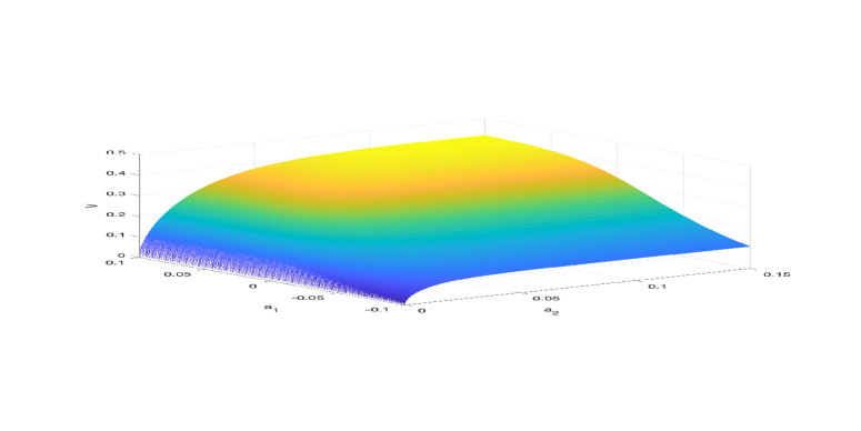
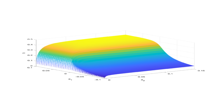
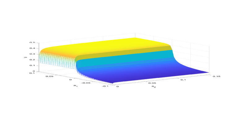
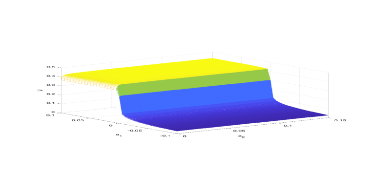
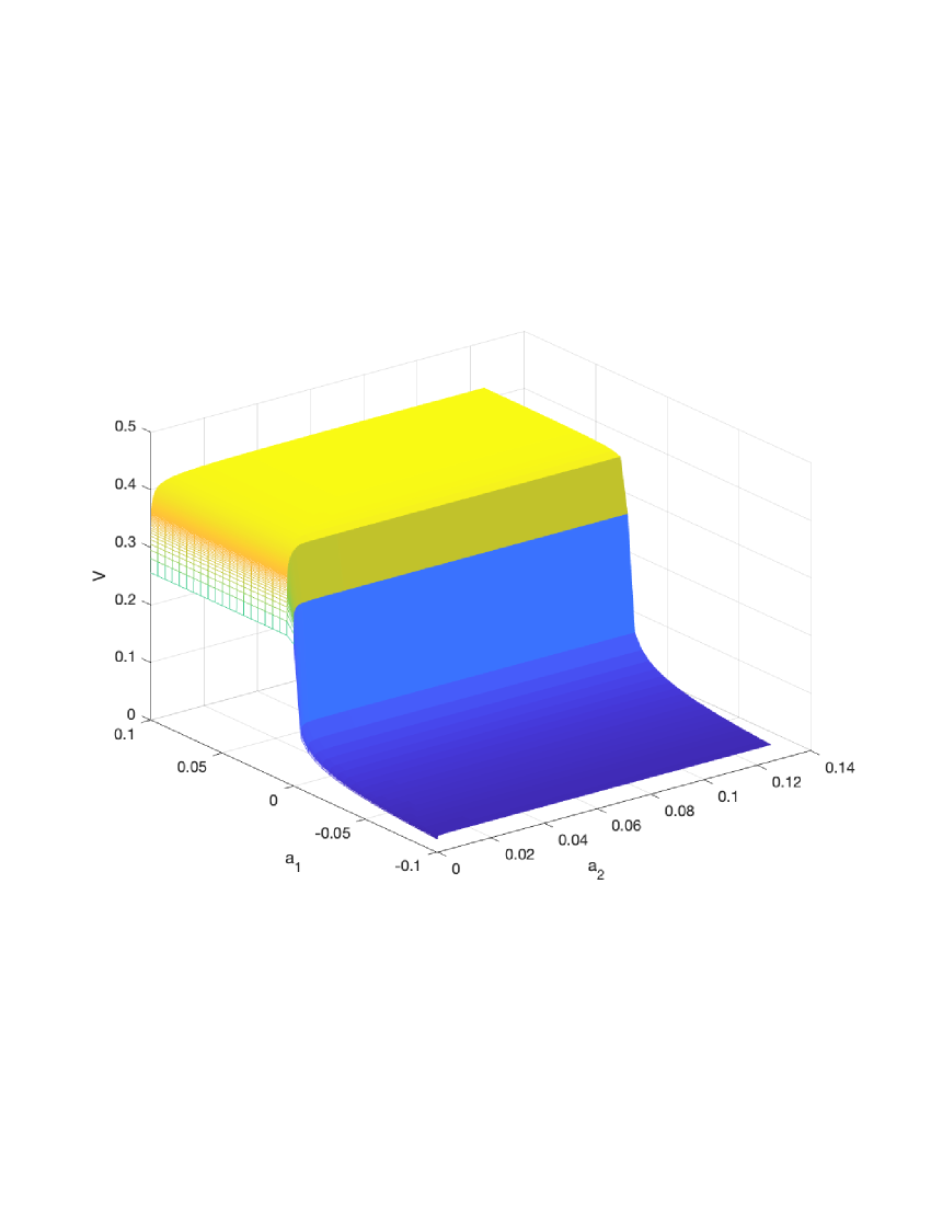
In an example shown in Fig. 1, DISC-GWR is used with the uniform grid; the step is $6.125\cdot 10^{-5}$, and the total CPU time for calculation of values at 98,400 points is of the order of 110-120 sec. for all 4 cases $\nu=1.2,0.8,0.5,0.3$.222The calculations in the paper were performed in MATLAB R2023b-academic use, on a MacPro Chip Apple M1 Max Pro chip with 10-core CPU, 24-core GPU, 16-core Neural Engine 32GB unified memory, 1TB SSD storage. The CPU times shown can be significantly improved using parallelized calculations. The accuracy decreases as $\nu$ decreases, and for $\nu=0.2$ (not shown), the best accuracy achievable using double precision arithmetic is several percent and more. Fig. 1 illustrates the reason: as $\nu$ decreases, the discretization error increases because the regularity of the probability distribution decreases. In all 4 cases, the value of $V$ at $a_{2}=0$ is zero but even at a distance $6.125*10^{-5}$ from 0, the value is non-negligible and increases as $\nu$ decreases; the derivative w.r.t. $a_{2}$ tends to infinity as $a_{2}\downarrow 0$ in all 4 cases. Fig. 2 demonstrates that if $\nu=0.3$, the cpdf is not small even at $a_{2}=1.5625*10^{-5}$. The accuracy of SINH-method decreases with $\nu$ as well but the accuracy of the order of $10^{-3}$ is achievable even in the case $\nu=0.2$ because all calculations are in the dual space.

The rest of the paper is organized as follows. In Sect. 2, we recall the definition of SINH-regular processes and SL-regular processes, formulas for the Laplace transforms of $V_{f.t.d.}(h,t)$, $V_{2}(a_{1},h;T)$ in terms of the expected present value operators, and various formulas for the Wiener-Hopf factors. We also study the regularity of the Wiener-Hopf factors. In Sect. 3, we list integral representations for $V_{f.t.d.}(h,t)$, $V_{2}(a_{1},h;T)$ and $\partial_{h}V_{2}(a_{1},h;T)$. In the same section, we outline other popular methods for pricing barrier options which can be used instead of the method of [8] and explain the difficulties that these methods face. Explicit formulas of the SINH-method are derived in Sect. 4. The algorithms and numerical examples are in Sect. 5. In Section 6, we summarise the results of the paper, In the appendix, we recall basic formulas and properties of the infinite trapezoid rule, summation by parts and GWR algorithm.

2. Classes of processes and formulas for the Wiener-Hopf factors

2.1. General classes of Lévy processes amenable to efficient calculations

For $\nu=0+$ (resp., $\nu=1+$), set $|\xi|^{\nu}=\ln|\xi|$ (resp., $|\xi|^{\nu}=|\xi|\ln|\xi|$), and introduce the following complete ordering in the set $\{0+,1+\}\cup(0,2]$: the usual ordering in $(0,2]$; $\forall\ \nu>0,0+<\nu$; $1<1+$; $\forall\ \nu>1,1+<\nu$. We use the notation $S_{(\mu_{-},\mu_{+})}=\{\xi\ |\ \operatorname{\rm Im}\xi\in(\mu_{-},\mu_{+})\}$, ${\mathcal{C}}_{\gamma_{-},\gamma_{+}}=\{e^{i\varphi}\rho\ |\ \rho>0,\varphi\in(\gamma_{-},\gamma_{+})\cup(\pi-\gamma_{+},\pi-\gamma_{-})\}$, ${\mathcal{C}}_{\gamma}=\{e^{i\varphi}\rho\ |\ \rho>0,\varphi\in(-\gamma,\gamma)\}$.

Definition 2.1.

([20, Defin. 2.1]) We say that $X$ is a SINH-regular Lévy process (on ${\mathbb{R}}$) of order $\nu$ and type $((\mu_{-},\mu_{+});{\mathcal{C}};{\mathcal{C}}_{+})$ iff the following conditions are satisfied:

  1. (i)

    $\nu\in\{0+,1+\}\cup(0,2]$ and $\mu_{-}<0<\mu_{+}$;

  2. (ii)

    ${\mathcal{C}}={\mathcal{C}}_{\gamma_{-},\gamma_{+}},{\mathcal{C}}_{+}={\mathcal{C}}_{\gamma^{\prime}_{-},\gamma^{\prime}_{+}}$, where $\gamma_{-}\leq\gamma^{\prime}_{-}<0<\gamma^{\prime}_{+}\leq\gamma_{+}$;

  3. (iii)

    the characteristic exponent $\psi$ of $X$ admits the representation

    (2.1) $$\psi(\xi)=-i\mu\xi+\psi^{0}(\xi),$$

    where $\mu\in{\mathbb{R}}$, and $\psi^{0}$ admits analytic continuation to $i(\mu_{-},\mu_{+})+({\mathcal{C}}\cup\{0\})$;

  4. (iv)

    for any $\varphi\in(\gamma_{-},\gamma_{+})$, there exists $c_{\infty}(\varphi)\in{\mathbb{C}}\setminus(-\infty,0]$ s.t.

    (2.2) $$\psi^{0}(\rho e^{i\varphi})\sim c_{\infty}(\varphi)\rho^{\nu},\quad\rho\to+\infty;$$
  5. (v)

    the function $(\gamma_{-},\gamma_{+})\ni\varphi\mapsto c_{\infty}(\varphi)\in{\mathbb{C}}$ is continuous;

  6. (vi)

    for any $\varphi\in(\gamma^{\prime}_{-},\gamma^{\prime}_{+})$, $\operatorname{\rm Re}c_{\infty}(\varphi)>0$.

Example 2.2.

A generic process of Koponen’s family was constructed in [9, 10] as pure jump processes with the Lévy measure of the form

(2.3) $$F(dx)=c_{+}e^{\lambda_{-}x}x^{-\nu_{+}-1}{\bf 1}_{(0,+\infty)}(x)dx+c_{-}e^{\lambda_{+}x}|x|^{-\nu_{-}-1}{\bf 1}_{(-\infty,0)}(x)dx,$$

where $c_{\pm}>0,\nu_{\pm}\in[0,2),\lambda_{-}<0<\lambda_{+}$. If $\nu_{\pm}\in(0,2),\nu_{\pm}\neq 1$,

(2.4) $$\psi^{0}(\xi)=c_{+}\Gamma(-\nu_{+})((-\lambda_{-})^{\nu_{+}}-(-\lambda_{-}-i\xi)^{\nu_{+}})+c_{-}\Gamma(-\nu_{-})(\lambda_{+}^{\nu_{-}}-(\lambda_{+}+i\xi)^{\nu_{-}}).$$

Note that a specialization $\nu_{\pm}=\nu\neq 1$, $c=c_{\pm}>0$, of KoBoL used in a series of numerical examples in [9] was named CGMY model in [23] (and the labels were changed: letters $C,G,M,Y$ replace the parameters $c,\nu,\lambda_{-},\lambda_{+}$ of KoBoL):

(2.5) $$\psi^{0}(\xi)=c\Gamma(-\nu)[(-\lambda_{-})^{\nu}-(-\lambda_{-}-i\xi)^{\nu}+\lambda_{+}^{\nu}-(\lambda_{+}+i\xi)^{\nu}].$$

Evidently, $\psi^{0}$ given by (2.5) is analytic in ${\mathbb{C}}\setminus i{\mathbb{R}}$, and $\forall\ \varphi\in(-\pi/2,\pi/2)$, (2.2) holds with

(2.6) $$c_{\infty}(\varphi)=-2c\Gamma(-\nu)\cos(\nu\pi/2)e^{i\nu\varphi}.$$

In [20], we defined a class of Stieltjes-Lévy processes (SL-processes). In order to save space, we do not reproduce the complete set of definitions. Essentially, $X$ is called a (signed) SL-process if $\psi$ is of the form

(2.7) $$\psi(\xi)=(a^{+}_{2}\xi^{2}-ia^{+}_{1}\xi)ST({\mathcal{G}}^{0}_{+})(-i\xi)+(a^{-}_{2}\xi^{2}+ia^{-}_{1}\xi)ST({\mathcal{G}}^{0}_{-})(i\xi)+(\sigma^{2}/2)\xi^{2}-i\mu\xi,$$

where $ST({\mathcal{G}})$ is the Stieltjes transform of a (signed) Stieltjes measure ${\mathcal{G}}$, $a^{\pm}_{j}\geq 0$, and $\sigma^{2}\geq 0$, $\mu\in{\mathbb{R}}$. We call a (signed) SL-process $X$ SL-regular if $X$ is SINH-regular. We proved in [20] that if $X$ is a (signed) SL-process then $\psi$ admits analytic continuation to the complex plane with two cuts along the imaginary axis, and if $X$ is a SL-process, then, for any $q>0$, equation $q+\psi(\xi)=0$ has no solution on ${\mathbb{C}}\setminus i{\mathbb{R}}$. We also proved that all popular classes of Lévy processes bar the Merton model and Meixner processes are regular SL-processes, with $\gamma_{\pm}=\pm\pi/2$; the Merton model and Meixner processes are regular signed SL-processes, and $\gamma_{\pm}=\pm\pi/4$. For lists of SINH-processes and SL-processes, with calculations of the order and type, see [20].

Note the following simple but important property of the characteristic exponent of a SINH-regular process, which is immediate from the Cauchy integral formula.

Lemma 2.3.

Let $X$ be a SINH-regular Lévy process (on ${\mathbb{R}}$) of order $\nu$ and type $((\mu_{-},\mu_{+});{\mathcal{C}};{\mathcal{C}}_{+})$. Then for any closed cone ${\mathcal{C}}^{\prime}\subset({\mathbb{C}}\cup\{0\})$, segment $[\mu^{\prime}_{-},\mu^{\prime}_{+}]\subset(\mu_{-},\mu_{+})$ and $n\in{\mathbb{Z}}_{+}$, there exists $C_{n}(\mu^{\prime}_{-},\mu^{\prime}_{+},{\mathcal{C}}^{\prime})$ such that

(2.8) $$|(\psi^{0})^{(n)}(\xi)|\leq C_{n}(\mu^{\prime}_{-},\mu^{\prime}_{+},{\mathcal{C}}^{\prime})(1+|\xi|)^{\nu-n},\ \xi\in i[\mu^{\prime}_{-},\mu^{\prime}_{+}]+{\mathcal{C}}^{\prime}.$$

2.2. Wiener-Hopf factorization and the Laplace transform of $V_{f.t.d.}(h,t)$ and $V_{2}(a_{1},h;T)$

For $q>0$, let $T_{q}$ be an exponentially distributed random variable of mean $1/q$, independent of $X$. For $\xi\in{\mathbb{R}}$, set ${\phi^{+}_{q}}(\xi)={\mathbb{E}}[e^{i{\bar{X}}_{T_{q}}\xi}]$ and ${\phi^{-}_{q}}(\xi)={\mathbb{E}}[e^{i{\underline{X}}_{T_{q}}\xi}]$. The Wiener-Hopf factorization formula is

(2.9) $$\frac{q}{q+\psi(\xi)}={\phi^{+}_{q}}(\xi){\phi^{-}_{q}}(\xi),\ \xi\in{\mathbb{R}}$$

(see, e.g. [33, p.81])). Define the (normalized) expected present value operators (EPV-operators) ${\mathcal{E}}^{\pm}_{q}$ and ${\mathcal{E}_{q}}$ by ${\mathcal{E}^{+}_{q}}u(x)={\mathbb{E}}[u(x+{\bar{X}}_{T_{q}})],$ ${\mathcal{E}^{-}_{q}}u(x)={\mathbb{E}}[u(x+{\underline{X}}_{T_{q}})],$ and ${\mathcal{E}_{q}}u(x)={\mathbb{E}}[u(x+X_{T_{q}})]$. Operators ${\mathcal{E}}^{\pm}_{q}$ and ${\mathcal{E}_{q}}$ are pseudo-differential operators (pdo) with the symbols $\phi^{\pm}_{q}(\xi)$ and $q/(q+\psi(\xi))$, respectively. Evidently, the EPV operators are bounded operators in $L_{\infty}({\mathbb{R}})$; if $\psi$ admits analytic continuation to a strip around the real axis, the EPV-operators act in spaces with exponential weights [12, 11]. In [12, 11], using the operator analog ${\mathcal{E}_{q}}={\mathcal{E}^{+}_{q}}{\mathcal{E}^{-}_{q}}={\mathcal{E}^{-}_{q}}{\mathcal{E}^{+}_{q}}$ of (2.9), we derived general pricing formulas for barrier options and first touch digitals, for a wide class of regular Lévy processes of exponential type (RLPE). The first step is the evaluation of the corresponding perpetual options, equivalently, calculation of the Laplace transform of the option price w.r.t. time to maturity, for positive values of the spectral parameter. In [8], the formulas for the perpetual barrier options are generalized for arbitrary Lévy process. We list the special cases of mirror reflections of Lemmas 2.1, 2.3 in [8] sufficient for the purposes of the present paper.

For $h\in{\mathbb{R}}$, let $\tau^{+}_{h}$ denote the first entry time by $X$ into $[h,+\infty)$.

Lemma 2.4.

Let $q>0$, $h>0$ and $G\in L_{\infty}$. Then

(2.10) $\displaystyle{\mathbb{E}}[\tau^{+}_{h}\leq T_{q}\ |\ X_{0}=0]$ $\displaystyle=$ $\displaystyle({\mathcal{E}^{+}_{q}}{\bf 1}_{[h,+\infty)})(0),$
(2.11) $\displaystyle{\mathbb{E}}[G(X_{T_{q}}){\bf 1}_{(-\infty,h]}({\bar{X}}_{T_{q}})\ |\ X_{0}={\bar{X}}_{0}=0]$ $\displaystyle=$ $\displaystyle({\mathcal{E}^{+}_{q}}{\bf 1}_{(-\infty,h]}{\mathcal{E}^{-}_{q}}G)(0).$

In particular, for $a\leq h$,

(2.12) $${\mathbb{E}}[{\bf 1}_{(-\infty,a]}(X_{T_{q}}){\bf 1}_{(-\infty,h]}({\bar{X}}_{T_{q}})\ |\ X_{0}={\bar{X}}_{0}=0]=({\mathcal{E}^{+}_{q}}{\bf 1}_{(-\infty,h]}{\mathcal{E}^{-}_{q}}{\bf 1}_{(-\infty,a]})(0).$$

It follows from (2.10) and (2.12) that, for $q>0$, the Laplace transforms of $V_{f.t.d}(h,t)$ and $V_{2}(a_{1},h;T)$ w.r.t. $t$ and $T$, respectively, are given by

(2.13) $\displaystyle{\tilde{V}}_{f.t.d}(h,q)$ $\displaystyle=$ $\displaystyle q^{-1}({\mathcal{E}^{+}_{q}}{\bf 1}_{[h,+\infty)})(0),$
(2.14) $\displaystyle{\tilde{V}}_{2}(a_{1},h;q)$ $\displaystyle=$ $\displaystyle-q^{-1}({\mathcal{E}^{+}_{q}}{\bf 1}_{[h,+\infty)}{\mathcal{E}^{-}_{q}}{\bf 1}_{(-\infty,a_{1}]})(0).$

It is evident that each side of (2.13) and (2.14) admits analytic continuation w.r.t. $q$ to $\{\operatorname{\rm Re}q>0\}$, therefore, one can recover $V_{f.t.d.}(h,t)$ and $V_{2}(a_{1},h;T)$ using the Bromwich integral:

(2.15) $$V(T)=\frac{1}{2\pi i}\int_{\operatorname{\rm Im}q=\sigma}\frac{e^{qT}}{q}{\tilde{V}}(q)dq,$$

for $T>0$ and any $\sigma>0$. Unless the function $V$ is sufficiently regular, the representation (2.15) is valid in the sense of the generalized functions only. To study the regularity of ${\tilde{V}}_{f.t.d}(h,q)$ and ${\tilde{V}}_{2}(a_{1},h;q)$ and design numerical procedures, we expand the indicator functions in (2.13) and (2.14) into the Fourier integrals, and use the following integral representations and properties of $\phi^{\pm}_{q}(\xi)$ (see, e.g., [12, 8, 14, 32, 17, 18]).

Lemma 2.5.

Let there exist $\mu_{-}\leq 0\leq\mu_{+}$, $\mu_{-}<\mu_{+}$, such that ${\mathbb{E}}[e^{-\gamma X_{1}}]<\infty$, $\forall\ \gamma\in[\mu_{-},\mu_{+}]$.

Then

  1. (i)

    $\psi(\xi)$ admits analytic continuation333Recall that a function $f$ is said to be analytic in the closure of an open set $U$ if $f$ is analytic in the interior of $U$ and continuous up to the boundary of $U$. to the strip $S_{[\mu_{-},\mu_{+}]}:=\{\xi\in{\mathbb{C}}\ |\ \operatorname{\rm Im}\xi\in[\mu_{-},\mu_{+}]\}$;

  2. (ii)

    let $\sigma>\max\{-\psi(i\mu_{-}),-\psi(i\mu_{+})\}$. Then there exists $c>0$ s.t. $|q+\psi(\xi)|\geq c$ for $q\geq\sigma$ and $\xi\in S_{[\mu_{-},\mu_{+}]}$;

  3. (iii)

    let $q\geq\sigma$. Then ${\phi^{+}_{q}}(\xi)$ (resp., ${\phi^{-}_{q}}(\xi)$) admits analytic continuation to $\{\operatorname{\rm Im}\xi\geq\mu_{-}\}$ (resp., $\{\operatorname{\rm Im}\xi\leq\mu_{+}\}$) given by

    (2.16) $\displaystyle{\phi^{+}_{q}}(\xi)$ $\displaystyle=$ $\displaystyle\frac{q}{(q+\psi(\xi)){\phi^{-}_{q}}(\xi)},\ \operatorname{\rm Im}\xi\in[\mu_{-},0],$
    (2.17) $\displaystyle{\phi^{-}_{q}}(\xi)$ $\displaystyle=$ $\displaystyle\frac{q}{(q+\psi(\xi)){\phi^{+}_{q}}(\xi)},\ \operatorname{\rm Im}\xi\in[0,\mu_{+}];$
  4. (iv)

    ${\phi^{+}_{q}}(\xi)$ (resp., ${\phi^{-}_{q}}(\xi)$) is uniformly bounded on $\{\operatorname{\rm Im}\xi\geq\mu_{-}\}$ (resp., $\{\operatorname{\rm Im}\xi\leq\mu_{+}\}$).

Lemma 2.6.

Let $\mu_{\pm}$, $X$ and $q$ satisfy the conditions of Lemma 2.5. Then

  1. (a)

    for any $\omega_{-}\in(\mu_{-},\mu_{+})$ and $\xi\in\{\operatorname{\rm Im}\xi>\omega_{-}\}$,

    (2.18) $${\phi^{+}_{q}}(\xi)=\exp\left[\frac{1}{2\pi i}\int_{\operatorname{\rm Im}\eta=\omega_{-}}\frac{\xi\ln(1+\psi(\eta)/q)}{\eta(\xi-\eta)}d\eta\right];$$
  2. (b)

    for any $\omega_{+}\in(\mu_{-},\mu_{+})$ and $\xi\in\{\operatorname{\rm Im}\xi<\omega_{+}\}$,

    (2.19) $${\phi^{-}_{q}}(\xi)=\exp\left[-\frac{1}{2\pi i}\int_{\operatorname{\rm Im}\eta=\omega_{+}}\frac{\xi\ln(1+\psi(\eta)/q)}{\eta(\xi-\eta)}d\eta\right].$$

The integrands above decay very slowly at infinity, hence, fast and accurate numerical realizations are impossible unless additional tricks are used. If $X$ is SINH-regular, the rate of decay can be greatly increased using appropriate conformal deformations of the line of integration and the corresponding changes of variables. Assuming that in Definition 2.1, $\gamma_{\pm}$ are not extremely small in absolute value (and, in the case of regular SL-processes, $\gamma_{\pm}=\pm\pi/2$ are not small), the most efficient change of variables is the sinh-acceleration

(2.20) $$\eta=\chi_{\omega_{1},b,\omega}(y)=i\omega_{1}+b\sinh(i\omega+y),$$

where $\omega\in(-\pi/2,\pi/2)$, $\omega_{1}\in{\mathbb{R}},b>0$. Typically, the sinh-acceleration is the best choice even if $|\gamma_{\pm}|$ are of the order of $10^{-5}$. The parameters $\omega_{1},b,\omega$ are chosen so that the contour ${\mathcal{L}}_{\omega_{1},b,\omega}:=\chi_{\omega_{1},b,\omega}({\mathbb{R}})\subset i(\mu_{+},\mu_{+})+({\mathcal{C}}_{\gamma_{-},\gamma_{+}}\cup\{0\})$ and, in the process of deformation, $\ln(1+\psi(\eta)/q)$ is a well-defined analytic function on a domain in ${\mathbb{C}}$ or the appropriate Riemann surface. We write ${\mathcal{L}}^{\pm}_{\omega_{1},b,\omega}$ or ${\mathcal{L}}^{\pm}$ instead ${\mathcal{L}}_{\omega_{1},b,\omega}$ when we wish to indicate that $\pm\omega>0$. Note that the wings of contours of type ${\mathcal{L}}^{+}_{\omega_{1},b,\omega}$ (resp., ${\mathcal{L}}^{-}_{\omega_{1},b,\omega}$) point upwards (respectively, downwards).

Lemma 2.7.

Let $X$ be SINH-regular of type $((\mu_{-},\mu_{+}),{\mathcal{C}}_{\gamma_{-},\gamma_{+}},{\mathcal{C}}_{\gamma^{\prime}_{-},\gamma^{\prime}_{+}})$.

Then there exists $\sigma>0$ s.t. for all $q>\sigma$,

  1. (i)

    ${\phi^{+}_{q}}(\xi)$ admits analytic continuation to $i(\mu_{-},+\infty)+i({\mathcal{C}}_{\pi/2-\gamma_{-}}\cup\{0\})$. For any $\xi\in i(\mu_{-},+\infty)+i({\mathcal{C}}_{\pi/2-\gamma_{-}}\cup\{0\})$, and any contour ${\mathcal{L}}^{-}_{\omega_{1},b,\omega}\subset i(\mu_{-},\mu_{+})+({\mathcal{C}}_{\gamma_{-},\gamma_{+}}\cup\{0\})$ lying below $\xi$,

    (2.21) $${\phi^{+}_{q}}(\xi)=\exp\left[\frac{1}{2\pi i}\int_{{\mathcal{L}}^{-}_{\omega_{1},b,\omega}}\frac{\xi\ln(1+\psi(\eta)/q)}{\eta(\xi-\eta)}d\eta\right];$$
  2. (ii)

    ${\phi^{-}_{q}}(\xi)$ admits analytic continuation to $i(-\infty,\mu_{+})-i({\mathcal{C}}_{\pi/2+\gamma_{+}}\cup\{0\})$. For any $\xi\in i(\-\infty,\mu_{+})-i({\mathcal{C}}_{\pi/2+\gamma_{+}}\cup\{0\})$, and any contour ${\mathcal{L}}^{+}_{\omega_{1},\omega,b}\subset i(\mu_{-},\mu_{+})+({\mathcal{C}}_{\gamma_{-},\gamma_{+}}\cup\{0\})$ lying above $\xi$,

    (2.22) $${\phi^{-}_{q}}(\xi)=\exp\left[-\frac{1}{2\pi i}\int_{{\mathcal{L}}^{+}_{\omega_{1},\omega,b}}\frac{\xi\ln(1+\psi(\eta)/q)}{\eta(\xi-\eta)}d\eta\right].$$

The integrals are efficiently evaluated making the change of variables $\eta=\chi_{\omega_{1},b,\omega}(y)$ and applying the simplified trapezoid rule.

Remark 2.1.

In the process of deformation, the expression $1+\psi(\eta)/q$ may not assume value zero. In order to avoid complications stemming from analytic continuation to an appropriate Riemann surface, it is advisable to ensure that $1+\psi(\eta)/q\not\in(-\infty,0]$. Thus, if $q>0$ - and only positive $q$’s are used in the Gaver-Stehfest method or GWR algorithm - and $X$ is an SL-process, any $\omega\in(0,\pi/2)$ is admissible in (2.21), and any $\omega\in(-\pi/2,0)$ is admissible in (2.22). If the sinh-acceleration is applied to the Bromwich integral, then additional conditions on $\omega$ must be imposed. See Sect. 2.4.

2.3. Decomposition of the Wiener-Hopf factors

In the remaining part of the paper, we assume that the Wiener-Hopf factors $\phi^{\pm}_{q}(\xi),q>0,$ admit the representations $\phi^{\pm}_{q}(\xi)=a^{\pm}_{q}+\phi^{\pm\pm}_{q}(\xi)$ and ${\mathcal{E}}^{\pm}_{q}=a^{\pm}_{q}I+{\mathcal{E}}^{\pm\pm}_{q}$, where $a^{\pm}_{q}\geq 0$, and $\phi^{\pm\pm}_{q}(\xi)$ satisfy the bounds

(2.23) $\displaystyle|\phi^{++}_{q}(\xi)|$ $\displaystyle\leq$ $\displaystyle C_{+}(q)(1+|\xi|)^{-\nu_{+}},\ \operatorname{\rm Im}\xi\geq\mu_{-},$
(2.24) $\displaystyle|\phi^{--}_{q}(\xi)|$ $\displaystyle\leq$ $\displaystyle C_{+}(q)(1+|\xi|)^{-\nu_{-}},\ \operatorname{\rm Im}\xi\leq\mu_{+},$

where $\nu_{\pm}>0$ and $C_{\pm}(q)>0$ are independent of $\xi$. These conditions are satisfied for all popular classes of Lévy processes bar the driftless Variance Gamma model.

The following more detailed properties of the Wiener-Hopf factors are established in [12, 13, 11] for the class of RLPE (Regular Lévy processes of exponential type); the proof for SINH-regular processes is the same only $\xi$ is allowed to tend to $\infty$ not only in the strip of analyticity but in the union of a strip and cone. See [7, 30, 32] for the proof of the statements below for several classes of SINH-regular processes (the definition of the SINH-regular processes formalizing properties used in [7, 30, 32] was suggested in [15] later). The contours in Lemma 2.8 below are in a domain of analyticity s.t. $q-i\mu\xi\neq 0$ and $1+\psi^{0}(\xi)/(q-i\mu\xi)\not\in(-\infty,0]$. These restrictions on the contours are needed when $\psi^{0}(\xi)=O(|\xi|^{\nu})$ as $\xi\to\infty$ in the domain of analyticity and $\nu<1$. Clearly, in this case, for sufficiently large $q>0$, the condition holds. If $X$ is an RLPE but not SINH-regular, the contours of integration in the lemma below are straight lines in the strip of analyticity.

Lemma 2.8.

Let $\mu_{-}<0<\mu_{+}$, $q>0$, let $X$ be SINH-regular of type $((\mu_{-},\mu_{+}),{\mathcal{C}}_{\gamma_{-},\gamma_{+}},{\mathcal{C}}_{\gamma^{\prime}_{-},\gamma^{\prime}_{+}})$, and order $\nu$. Then

  1. (1)

    if $\nu\in[1,2]$ or $\nu\in(0,1)$ and the drift $\mu=0$, then neither ${\bar{X}}_{T_{q}}$ nor ${\underline{X}}_{T_{q}}$ has an atom at 0, and $\phi^{\pm}_{q}(\xi)$ admit the bounds (2.23) and (2.24), where $\nu_{\pm}>0$ and $C_{\pm}(q)>0$ are independent of $\xi$;

  2. (2)

    if $\nu\in[0+,1)$ and $\mu>0$, then

    1. (a)

      ${\bar{X}}_{T_{q}}$ has no atom at 0 and ${\underline{X}}_{T_{q}}$ has an atom $a^{-}_{q}\delta_{0}$ at zero, where

      (2.25) $$a^{-}_{q}=\exp\left[-\frac{1}{2\pi i}\int_{{\mathcal{L}}^{+}_{\omega_{1},b,\omega}}\frac{\ln((1+\psi^{0}(\eta)/(q-i\mu\eta))}{\eta}d\eta\right],$$

      and ${\mathcal{L}}^{+}_{\omega_{1},b,\omega}$ is a contour as in Lemma 2.7 (ii);

    2. (b)

      for $\xi$ and ${\mathcal{L}}^{-}_{\omega_{1},b,\omega}$ in Lemma 2.7 (i), ${\phi^{+}_{q}}(\xi)$ admits the representation

      (2.26) $${\phi^{+}_{q}}(\xi)=\frac{q}{q-i\mu\xi}\exp\left[\frac{1}{2\pi i}\int_{{\mathcal{L}}^{-}_{\omega_{1},b,\omega}}\frac{\xi\ln(1+\psi^{0}(\eta)/(q-i\mu\eta))}{\eta(\xi-\eta)}d\eta\right],$$

      and satisfies the bound (2.23) with $\nu_{+}=1$;

    3. (c)

      ${\phi^{-}_{q}}(\xi)=a^{-}_{q}+\phi^{--}_{q}(\xi)$, where $\phi^{--}_{q}(\xi)$ satisfies (2.24) with arbitrary $\nu_{-}\in(0,1-\nu)$;

    4. (d)

      ${\mathcal{E}^{-}_{q}}=a^{-}_{q}I+{\mathcal{E}}^{--}_{q}$, where ${\mathcal{E}}^{--}_{q}$ is the pdo with the symbol $\phi^{--}_{q}(\xi)$;

  3. (3)

    if $\nu\in[0+,1)$ and $\mu<0$, then

    1. (a)

      ${\underline{X}}_{T_{q}}$ has no atom at 0 and ${\bar{X}}_{T_{q}}$ has an atom $a^{+}_{q}\delta_{0}$ at zero, where

      (2.27) $$a^{+}_{q}=\exp\left[\frac{1}{2\pi i}\int_{{\mathcal{L}}^{-}_{\omega_{1},b,\omega}}\frac{\ln((1+\psi^{0}(\eta)/(q-i\mu\eta))}{\eta}d\eta\right],$$

      and ${\mathcal{L}}^{-}_{\omega_{1},b,\omega}$ is a contour as in Lemma 2.7 (i);

    2. (b)

      for $\xi$ and ${\mathcal{L}}^{+}_{\omega_{1},b,\omega}$ in Lemma 2.7 (ii), ${\phi^{-}_{q}}(\xi)$ admits the representation

      (2.28) $${\phi^{-}_{q}}(\xi)=\frac{q}{q-i\mu\xi}\exp\left[-\frac{1}{2\pi i}\int_{{\mathcal{L}}^{+}_{\omega_{1},b,\omega}}\frac{\xi\ln(1+\psi^{0}(\eta)/(q-i\mu\eta))}{\eta(\xi-\eta)}d\eta\right],$$

      and satisfies the bound (2.24) with $\nu_{-}=1$;

    3. (c)

      ${\phi^{+}_{q}}(\xi)=a^{+}_{q}+\phi^{++}_{q}(\xi)$, where $\phi^{++}_{q}(\xi)$ satisfies (2.23) with arbitrary $\nu_{+}\in(0,1-\nu)$;

    4. (d)

      ${\mathcal{E}^{+}_{q}}=a^{+}_{q}I+{\mathcal{E}}^{++}_{q}$, where ${\mathcal{E}}^{++}_{q}$ is the pdo with the symbol $\phi^{++}_{q}(\xi)$.

2.4. Analytic continuation w.r.t. $q$

It is easy to see that, given a strip of analyticity $S_{[\mu^{\prime}_{-},\mu^{\prime}_{+}]}$, $\mu^{\prime}_{-}<0<\mu^{\prime}_{+}$, of $\psi$, one can find $\sigma_{0}>0$ such that both ${\phi^{+}_{q}}(\xi)$ and ${\phi^{-}_{q}}(\xi)$ are uniformly bounded on ${\mathcal{U}}(\sigma;\mu^{\prime}_{-},\mu^{\prime}_{+}):=\{\operatorname{\rm Re}q\geq\sigma_{0},\operatorname{\rm Im}\xi\in[\mu^{\prime}_{-},\mu^{\prime}_{+}]\}$, $\operatorname{\rm Re}(q+\psi(\xi))$ is positive on ${\mathcal{U}}(\sigma;\mu^{\prime}_{-},\mu^{\prime}_{+})$, and the functions in the formulas for $\phi^{\pm}_{q}(\xi)$ above, with flat contours of integration, admit analytic continuation to ${\mathcal{U}}(\sigma;\mu^{\prime}_{-},\mu^{\prime}_{+})$. Therefore, any formula for the Laplace transforms ${\tilde{V}}(q)$ of expectations of random variables which we use or derive below in terms of the Wiener-Hopf factors can be used to define analytic continuation of ${\tilde{V}}(q)$ to the half-plane $\{\operatorname{\rm Re}q\geq\sigma_{0}\}$ and use the Bromwich integral to recover $V$: for any $T>0$ and $\sigma\geq\sigma_{0}$, (2.15) holds. In order that a deformation of the contour in (2.15) can be justified, and a numerical procedure for the evaluation of the Bromwich integral (2.15) be reliable, it is necessary that ${\tilde{V}}(q)$ decay sufficiently fast as $q\to\infty$ along the contour of integration. For the proof, we use the integration by parts in the formula for ${\tilde{V}}(q)$ and the following lemma. First, we consider the case $\nu\in[1,2]$ or $\nu\in(0,1)$ and $\mu=0$. If $\nu\neq 1$, set $\nu_{\pm}=\nu/2$. If $\nu=1$, we assume that $c_{\infty}(\varphi)$ in (2.2) is of the form $c_{\infty}e^{i\varphi}$, then $(\nu_{+},\nu_{-})$ is the solution of the system $\nu_{+}+\nu_{-}=1,\nu_{+}-\nu_{-}=(2/\pi)\arctan(\mu/c_{\infty})$.

Lemma 2.9.

Let $X$ be a SINH-regular process. Let either the order $\nu\in[1,2]$ or $\nu\in(0,1)$ and the drift is 0. Then there exist $(\mu^{\prime}_{-},\mu^{\prime}_{+})\subset(\mu_{-},\mu_{+})$, $\mu^{\prime}_{-}<\mu^{\prime}_{+}$, a cone ${\mathcal{C}}_{\gamma^{\prime}_{-},\gamma^{\prime}_{+}}$, $\gamma^{\prime}_{-}<0<\gamma^{\prime}_{+}$, and $\sigma_{0}>0,\omega_{L}\in(0,\pi/2)$ such that

  1. (a)

    for all $q\in\sigma_{0}+{\mathcal{C}}_{\pi/2+\omega_{L}}$ and $\xi\in i(\mu^{\prime}_{-},\mu^{\prime}_{+})+({\mathcal{C}}_{\gamma^{\prime}_{-},\gamma^{\prime}_{+}}\cup\{0\})$,

    (2.29) $$q+\psi(\xi)\not\in(-\infty,0];$$
  2. (b)

    ${\phi^{+}_{q}}(\xi)$ admits analytic continuation to $(\sigma_{0}+{\mathcal{C}}_{\pi/2+\omega_{L}})\times(i(\mu,+\infty)+i({\mathcal{C}}_{\pi/2-\gamma^{\prime}_{-}}\cup\{0\}))$ and obeys the bounds

    (2.30) $\displaystyle|{\phi^{+}_{q}}(\xi)|$ $\displaystyle\leq$ $\displaystyle C_{+}(|q|^{1/\nu}+|\xi|)^{-\nu_{+}},$
    (2.31) $\displaystyle|\partial_{q}^{m}\partial^{n}_{\xi}{\phi^{+}_{q}}(\xi)|$ $\displaystyle\leq$ $\displaystyle C_{+,m,n}(|q|^{1/\nu}+|\xi|)^{-\nu_{+}}|q|^{-m}(1+|\xi|)^{-n},\ n,m\in{\mathbb{Z}}_{+},$

    where $C_{+},C_{+,m,n}$ are independent of $q,\xi$;

  3. (c)

    ${\phi^{-}_{q}}(\xi)$ admits analytic continuation to $(\sigma_{0}+{\mathcal{C}}_{\pi/2+\omega_{L}})\times(i(-\infty,\mu_{+})-i({\mathcal{C}}_{\pi/2+\gamma^{\prime}_{+}}\cup\{0\}))$ and obeys the bounds

    (2.32) $\displaystyle|{\phi^{+}_{q}}(\xi)|$ $\displaystyle\leq$ $\displaystyle C_{-}(|q|^{1/\nu}+|\xi|)^{-\nu_{-}},$
    (2.33) $\displaystyle|\partial_{q}^{m}\partial^{n}_{\xi}{\phi^{+}_{q}}(\xi)|$ $\displaystyle\leq$ $\displaystyle C_{-,m,n}(|q|^{1/\nu}+|\xi|)^{-\nu_{-}}|q|^{-m}(1+|\xi|)^{-n},$

    where $C_{+},C_{+,m,n}$ are independent of $q,\xi$.

Proof.

Eq. (2.29), (2.30) and (2.32) were derived and used in [12, 11, 7] for $\xi$ in a strip, and in [32] for $\xi$ in a union of a strip and cone. The bounds (2.30) and (2.32) (in a less explicit form) are proved and used in [17, 18]. The bounds (2.31) and (2.33) are immediate from (2.30), (2.32) and the Cauchy integral formula.

3. Evaluation and regularity of $V_{f.t.d.}(h,t)$, $V_{2}(a_{1},h;T)$, and $\partial_{h}V_{2}(a_{1},h;T)$

3.1. Representations and numerical evaluation of $V_{f.t.d.}(h,t)$

Let $h>0$ and let $\psi$ admit analytic continuation to $S_{(\mu_{-},0]}$. Then, for any $\omega_{-}\in(\mu_{-},0)$ and sufficiently large $\sigma$,

(3.1) $\displaystyle V_{f.t.d.}(h,t)$ $\displaystyle=$ $\displaystyle\frac{1}{2\pi i}\int_{\operatorname{\rm Re}q=\sigma}dq\frac{e^{qt}}{q}\frac{1}{2\pi}\int_{\operatorname{\rm Im}\xi=\omega_{-}}d\xi\,e^{-i\xi h}\frac{{\phi^{+}_{q}}(\xi)}{i\xi}$
(3.2) $\displaystyle=$ $\displaystyle\frac{1}{2\pi i}\int_{\operatorname{\rm Re}q=\sigma}dq\frac{e^{qt}}{q}\frac{1}{2\pi}\int_{\operatorname{\rm Im}\xi=\omega_{-}}d\xi\,e^{-i\xi h}\frac{\phi^{++}_{q}(\xi)}{i\xi}.$

If ${\phi^{+}_{q}}(\xi)\neq\phi^{++}_{q}(\xi)$, it is advantageous to use (3.2) rather than (3.1) because on the strength of (2.23), the integral on the RHS of (3.2) is absolutely convergent whereas the one on the RHS of (3.1) is not. If $X$ satisfies the conditions of Lemma 2.9, we can deform the inner contour into a contour of the form ${\mathcal{L}}^{-}_{\omega_{1},b,\omega}$:

(3.3) $$V_{f.t.d.}(h,t)=\frac{1}{2\pi i}\int_{\operatorname{\rm Re}q=\sigma}\frac{e^{qt}}{q}\frac{1}{2\pi}\int_{{\mathcal{L}}^{-}_{\omega_{1},b,\omega}}e^{-i\xi h}\frac{\phi^{++}_{q}(\xi)}{i\xi}d\xi,$$

make the corresponding sinh-change of variables, and apply the simplified trapezoid rule. For each $q$ used in a numerical method for the evaluation of the Bromwich integral, the error tolerance of the order of E-12-E-13 can be satisfied using the simplified trapezoid rule with 150-300 terms (the number depends on the properties of $\psi$, the opening angle of the sector of analyticity especially).

To calculate the outer integral, we apply the sinh-acceleration or summation by parts in the infinite trapezoid rule and truncate the sum. The error tolerance of the order of E-12 (resp., E-14) can be satisfied using a truncated sum with 150-200 (resp., 200-250) terms. We can also apply the GWR algorithm with $2M=16$ terms but then the best accuracy that can be achieved is of the order of E-07 unless high precision arithmetics and $2M>16$ are used.

Thus, if the order of the process $\nu\in[1,2]$ or $\nu\in(0,1)$ and $\mu=0$, we recommend to apply the sinh-acceleration to the outer integral as well:

(3.4) $$V_{f.t.d.}(h,t)=\frac{1}{2\pi i}\int_{{\mathcal{L}}^{L}_{\sigma,b_{\ell},\omega_{\ell}}}dq\frac{e^{qt}}{q}\frac{1}{2\pi}\int_{{\mathcal{L}}^{-}_{\omega_{1},b,\omega}}d\xi\,e^{-i\xi h}\frac{\phi^{++}_{q}(\xi)}{i\xi},$$

where ${\mathcal{L}}^{L}_{\sigma,b_{\ell},\omega_{\ell}}=\chi^{L}_{\sigma,b_{\ell},\omega_{\ell}}({\mathbb{R}})$ and $\chi^{L}_{\sigma,b_{\ell},\omega_{\ell}}(y)=\sigma+ib_{\ell}\sinh(i\omega_{\ell}+y)$. The parameters are chosen so that, for all $(q,\xi)$ arising in the process of deformations, $q+\psi(\xi)\not\in(-\infty,0]$. If $\nu\in(1,2]$ or $\nu\in(0,1]$ and $\mu=0$, the crucial parameters $\gamma_{-}<\omega<0$ and $0<\omega_{\ell}<\pi/2$ must satisfy $\max\{1,\nu\}|\omega|<\pi/2-\omega_{\ell}$ (if $\nu=1$ and $\mu\neq 0$, the condition is more involved). If $\max\{1,\nu\}|\omega|<\pi/2-\omega_{\ell}$, it is straightforward to show that there exist $\omega_{1},b,\sigma,b_{\ell}$ such that for all $(q,\xi)$ arising in the process of deformations, $q+\psi(\xi)\not\in(-\infty,0]$. For details, see [17, 18].

3.2. Representations and numerical evaluation of $V_{2}(a_{1},h;T)$

The following representation for $V_{2}(a_{1},h;T)$ is immediate from [18, Thm.3.5]:

Theorem 3.1.

Let $a_{1}\leq b$, $h>0$. For any $\mu_{-}<\omega_{-}<0<\omega_{+}<\mu_{+}$, there exists $\sigma_{0}>0$ such that, for any $q\geq\sigma_{0}$, the Laplace transform ${\tilde{V}}_{2}(a_{1},h;q)$ is given by

(3.5) $${\tilde{V}}_{2}(a_{1},h;T)=\frac{1}{(2\pi)^{2}q}\int_{\operatorname{\rm Im}\eta=\omega_{-}}d\eta\,e^{-ih\eta}\phi^{++}_{q}(\eta)\int_{\operatorname{\rm Im}\xi=\omega_{+}}d\xi\,\frac{e^{i\xi(h-a_{1})}\phi^{--}_{q}(\xi)}{\xi(\xi-\eta)}.$$

In [18], it is also proved that the integrand on the RHS of (3.5) is bounded (in absolute value) by an integrable function independent of $q\in\{\operatorname{\rm Re}q\geq\sigma_{0}\}$. Therefore, $V_{2}(a_{1},h;T)$ can be recovered using the Bromwich integral

$\displaystyle V_{2}(a_{1},h;T)$ $\displaystyle=$ $\displaystyle\frac{1}{2\pi i}\int_{\operatorname{\rm Re}q=\sigma}dq\,\frac{e^{qT}}{q}$
$\displaystyle\cdot\frac{1}{(2\pi)^{2}}\int_{\operatorname{\rm Im}\eta=\omega_{-}}d\eta\,e^{-ih\eta}\phi^{++}_{q}(\eta)\int_{\operatorname{\rm Im}\xi=\omega_{+}}d\xi\,\frac{e^{i\xi(h-a_{1})}\phi^{--}_{q}(\xi)}{\xi(\xi-\eta)}$

understood in the sense of generalized functions. Assuming that $\nu\in[1,2]$ or $\nu\in(0,1)$ and $\mu=0$, we can apply appropriate sinh-acceleration deformations to the integrals w.r.t. $q,\eta,\xi$:

$\displaystyle V_{2}(a_{1},h;T)$ $\displaystyle=$ $\displaystyle\frac{1}{2\pi i}\int_{{\mathcal{L}}^{L}_{\sigma,b_{\ell},\omega_{\ell}}}dq\,\frac{e^{qT}}{q}$
$\displaystyle\cdot\frac{1}{(2\pi)^{2}}\int_{{\mathcal{L}}^{-}_{\omega^{-}_{1},b^{-},\omega_{-}}}d\eta\,e^{-ih\eta}\phi^{++}_{q}(\eta)\int_{{\mathcal{L}}^{+}_{\omega^{+}_{1},b^{+},\omega_{+}}}\frac{e^{i\xi(h-a_{1})}\phi^{--}_{q}(\xi)d\xi\,}{\xi(\xi-\eta)}.$

For any compact subset of $\{a_{1}\leq h,h\geq 0,T\geq t>0\}$, the triple integrand is bounded in absolute value by a function of class $L_{1}$ (see [18] for the proof), hence, the function on the RHS is continuous on $\{a_{1}\leq h,h\geq 0,T>0\}$. We can also apply the GWR algorithm to the outer integral below

$\displaystyle V_{2}(a_{1},h;T)$ $\displaystyle=$ $\displaystyle\frac{1}{2\pi i}\int_{\operatorname{\rm Re}q=\sigma}dq\,\frac{e^{qT}}{q}$
$\displaystyle\cdot\frac{1}{(2\pi)^{2}}\int_{{\mathcal{L}}^{-}_{\omega^{-}_{1},b^{-},\omega_{-}}}d\eta\,e^{-ih\eta}\phi^{++}_{q}(\eta)\int_{{\mathcal{L}}^{+}_{\omega^{+}_{1},b^{+},\omega_{+}}}\frac{e^{i\xi(h-a_{1})}\phi^{--}_{q}(\xi)d\xi\,}{\xi(\xi-\eta)},$

Numerical examples in [18] demonstrate that the best accuracy achievable with the GWR algorithm is several orders of magnitude worse, and, for the same accuracy, the CPU times are approximately the same.

3.3. Representations of $\partial_{h}V_{2}(a_{1},h;T)$ and $\partial_{a_{1}}\partial_{h}V_{2}(a_{1},h;T)$

If $\nu\in[1,2]$ or $\nu\in(0,1)$ and $\mu=0$, the differentiation under the integral sign on the RHS of (3.2) is justified444The proof in [30] for several classes of SINH-regular processes is valid for all SINH-regular processes., and we obtain

$\displaystyle\partial_{h}V_{2}(a_{1},h;T)$ $\displaystyle=$ $\displaystyle\frac{1}{2\pi i}\int_{{\mathcal{L}}^{L}_{\sigma,b_{\ell},\omega_{\ell}}}dq\,\frac{e^{qT}}{q}$
$\displaystyle\cdot\frac{1}{(2\pi)^{2}}\int_{{\mathcal{L}}^{-}_{\omega^{-}_{1},b^{-},\omega_{-}}}d\eta\,e^{-ih\eta}\phi^{++}_{q}(\eta)\int_{{\mathcal{L}}^{+}_{\omega^{+}_{1},b^{+},\omega_{+}}}\frac{e^{i\xi(h-a_{1})}\phi^{--}_{q}(\xi)d\xi\,}{-i\xi},$

and

$\displaystyle\partial_{a_{1}}\partial_{h}V_{2}(a_{1},h;T)$ $\displaystyle=$ $\displaystyle\frac{1}{2\pi i}\int_{{\mathcal{L}}^{L}_{\sigma,b_{\ell},\omega_{\ell}}}dq\,\frac{e^{qT}}{q}\frac{1}{(2\pi)^{2}}\int_{{\mathcal{L}}^{-}_{\omega^{-}_{1},b^{-},\omega_{-}}}d\eta\,$
$\displaystyle\cdot e^{-ih\eta}\phi^{++}_{q}(\eta)\int_{{\mathcal{L}}^{+}_{\omega^{+}_{1},b^{+},\omega_{+}}}e^{i\xi(h-a_{1})}\phi^{--}_{q}(\xi)d\xi.$

In the general case, we can derive an analogue of (3.3) in the sense of the generalized functions only:

$\displaystyle\partial_{h}V_{2}(a_{1},h;T)$ $\displaystyle=$ $\displaystyle\frac{1}{2\pi i}\int_{\operatorname{\rm Re}q=\sigma}dq\,\frac{e^{qT}}{q}$
$\displaystyle\cdot\frac{1}{(2\pi)^{2}}\int_{\operatorname{\rm Im}\eta=\omega_{-}}d\eta\,e^{-ih\eta}\phi^{++}_{q}(\eta)\int_{\operatorname{\rm Im}\xi=\omega_{+}}\frac{e^{i\xi(h-a_{1})}\phi^{--}_{q}(\xi)d\xi\,}{-i\xi}.$
Remark 3.1.

As functions of $\xi$ on the contours that we consider, $\phi^{\pm\pm}_{q}(\xi)/\xi$ are absolutely integrable. In the result, in the formulas for $V_{f.t.d.}(h,t)$ and $V_{2}(a_{1},h;T)$, the integrand is absolutely integrable as a function of $\xi$. However, to make the integrand absolutely convergent as a function of $q$, we need to integrate by parts. Under conditions of Lemma 2.9, we can integrate by parts, and reduce the analysis to the case of the absolutely convergent multiple integrals. If $\nu<1$ and $\mu\neq 0$, then not only Lemma 2.9 is not applicable; one can show that the conclusions of the lemma fail. Hence, the formulas for $V_{f.t.d.}(h,t)$ and $V_{2}(a_{1},h;T)$, and, especially, for $\partial_{h}V_{2}(a_{1},h;T)$, can be understood in the sense of generalized functions only, and the proof of convergence and error bounds for standard quadratures are difficult.

3.4. Evaluation using Carr’s randomization

This problem does not arise if Carr’s randomization is applied because, at each step, prices of perpetual barrier options are calculated, and, for positive values of the spectral parameter, the Wiener-Hopf factors are sufficiently regular. Carr’s randomization algorithm (maturity randomization) is justified for Markov processes in [6], under a weak regularity condition, and applied to price barrier options in regime-switching hyper-exponential jump-diffusion models. In [8], explicit Carr’s randomization algorithms were developed for RLPE processes. The class of SINH-processes being a subclass of the class of RLPE processes, we can evaluate $V_{f.t.d.}(h,t)$ and $V(a_{1},h;T)$ using the method in [8]. In [30], the method is justified for sensitivities, hence, one can evaluate $\partial_{h}V(a_{1},h;T)$ as well. However, the calculations in [8] are in the state space, therefore, slower than the calculations in the dual space. Also, additional interpolation errors appear.

In Carr’s randomization approximation, the maturity period $T$ of the option is divided into $N$ subintervals, using points $0=t_{0}<t_{1}<\dotsb<t_{N}=T$ (when $V_{f.t.d.}(h,t)$ is calculated, $T=t$), and each sub-period $[t_{s},t_{s+1}]$ is replaced with an exponentially distributed random maturity period with mean $\Delta_{s}=t_{s+1}-t_{s}$. Moreover, these $N$ random maturity sub-periods are assumed to be independent of each other and of the process $X$. In [22], it is assumed that $\Delta_{s}=T/N$ for all $s$, but, in principle, it is unnecessary to impose this requirement. In [8], the killing rate (interest rate) $r$ is assumed positive but for options of finite maturity the proof and algorithms remain valid for any $r\in{\mathbb{R}}$. For the purposes of the present paper, we need $r=0$. Below, $V_{s}$ denotes the Carr’s randomization approximation to the value at time $t_{s}$. Algorithm for $V_{f.t.d.}(h,t;x)$, the price of the first touch digital at $X_{0}=x$. The maturity date $t$, the upper barrier $h$.

  1. I.

    Set $V_{N}={\bf 1}_{[h,+\infty)}$.

  2. II.

    For $s=N-1,N-2,\ldots,0$, calculate $q_{s}=t/\Delta_{s}$ and $V_{s}=(1/q_{s}){\bf 1}_{(\infty,h)}{\mathcal{E}}^{+}_{q_{s}}V_{s+1}+{\bf 1}_{[h,+\infty)}$.

  3. III.

    $V_{f.t.d.}(h,t;x)=V_{0}(x),x\in{\mathbb{R}}.$

Algorithm for $V_{joint}(a_{1},h;T,x)={\mathbb{P}}[X_{T}\leq a_{1},{\bar{X}}_{T}\leq h\ |\ X_{0}=x]$, $a_{1}\leq h$.

  1. I.

    Set $V_{N}={\bf 1}_{(-\infty,a_{1}]}$.

  2. II.

    For $s=N-1,N-2,\ldots,0$, calculate $q_{s}=T/\Delta_{s}$ and $V_{s}=(1/q_{s}){\mathcal{E}}^{+}_{q_{s}}{\bf 1}_{(-\infty,h]{\mathcal{E}}^{-}_{q_{s}}}V_{s+1}$.

  3. III.

    $V_{joint}(a_{1},h;T,x)=V_{0}(x),x\in{\mathbb{R}}.$

The values $V_{s}(x)$ are evaluated at points of a chosen grid using an appropriate piece-wise interpolation procedure. The state space is truncated, and the approximation to $V_{s}$ is represented by the array $\{V_{s;j}\}_{j=1}^{M}$ of the values $V_{s}(x_{j})$ at points of the chosen grid. The EPV-operators become the matrix operators, which can be efficiently realized using the fast convolution. See [8] for details. To be more specific, the matrix elements of the discretized ${\mathcal{E}}^{\pm}_{q}$ are linear combinations of reals of the form

(3.12) $\displaystyle({\mathcal{E}}^{\pm}_{q}{\bf 1}_{(-\infty,a]}(\cdot)^{n})(0)$ $\displaystyle=$ $\displaystyle\frac{(n-1)!}{2\pi}\int_{\operatorname{\rm Im}\xi=\omega_{-}}e^{-ia\xi}\phi^{\pm}_{q}(\xi)(i\xi)^{-n-1}d\xi,$
(3.13) $\displaystyle({\mathcal{E}}^{\pm}_{q}{\bf 1}_{[a,+\infty)}(\cdot)^{n})(0)$ $\displaystyle=$ $\displaystyle-\frac{(n-1)!}{2\pi}\int_{\operatorname{\rm Im}\xi=\omega_{+}}e^{-ia\xi}\phi^{\pm}_{q}(\xi)(i\xi)^{-n-1}d\xi,$

for $n\geq 0$, where $\omega_{-}<0$ and $0<\omega_{+}$ are sufficiently small in absolute value so that the contours $\{\operatorname{\rm Im}\xi=\omega_{\pm}\}$ are in the strip of analyticity of $\phi^{\pm}_{q}$. In [8], uniforms grids and the piece-wise linear interpolation is used, and the matrix elements of the discretized EPV-operators are calculated using the Fast Fourier transform (FFT). More accurate and faster calculations of the matrix elements can be performed using the sinh-acceleration similarly to [25] where the matrix elements of the discretized transition operators are calculated using fractional-parabolic deformations. If the process has a significant Brownian motion component or the characteristic exponent is a rational function, then the interpolation of higher order can be advantageous. See [25] for explicit formulas for the matrix elements.

If the value function is irregular, then, in a vicinity of the barrier, it is advantageous to approximate $V_{s}$ on $[h-2\Delta,h]$ as $V_{s}(x)\approx V_{s}(h-\Delta)$ instead of $V_{s}(x)\approx V_{s}(h-)+(x-h)(V_{s}(h-0),V_{s}(h-2\Delta))/2$. We leave to the reader the straightforward modification of the construction of the matrix approximation in [8].

Remark 3.2.
  1. (a)

    If the left tail of the distribution of $X$ decays very slowly, then it is necessary to use a very large truncated interval, and Carr’s randomization becomes very inefficient.

  2. (b)

    One can perform all steps of Carr’s randomization in the dual space using the fast Hilbert transform as in [27] were barrier options in the discrete time model are priced. However, $\phi^{\pm}_{q}(\xi)$ decay very slowly as $\xi\to\infty$, hence, extremely long grids are necessary to satisfy even a moderate error tolerance.

3.5. Other methods for pricing barrier options

If $\nu\in[1,2]$ or $\nu\in(0,1)$ and $\mu=0$, then the method of [18] based on the application of the sinh-acceleration to the Bromwich integral and the integrals w.r.t. other variables in the pricing formula is the most efficient. Several popular methods are based on either approximation of small jumps by an additional Brownian Motion component or by processes with rational characteristic exponents. The method of [18] is applicable after such an approximation555An approximation of a small jump component should be done so that the new process is SINH-regular. but the approximation error itself is, typically, sizable, because, implicitly, functions with the unbounded first derivative are approximated by smooth functions. See [28, 8] for examples of errors of Cont-Volchkova method (approximation of a small jump component) and approximation with the Hyper-Exponential jump-diffusion model, respectively. One can also approximate barrier options with continuous monitoring with barrier options with discrete monitoring, and use any method for pricing the latter, e.g., COS or BPROJ method, but both methods introduce additional errors. See [25, 21] for examples and qualitative analysis.

3.6. Regularity of $V_{f.t.d.}(h,t)$, $V_{2}(a_{1},h;T)$ and $\partial_{h}V_{2}(a_{1},h;T)$

In [12] and [7], the following asymptotic formulas were derived for $V_{f.t.d.}(h,t)$ and $V_{2}(a_{1},h;T)$, respectively (in both papers, the spot varies and barrier are fixed; we reformulate the results for the case when the spot 0 is fixed, and the barrier varies). In [30], the asymptotic formulas are derived for sensitivities.

Theorem 3.2.

Let $X$ be SINH-regular of order $\nu$, and $t>0,T>0$, $a_{1}\leq 0$ are fixed.

Then there exist $\kappa(t)>0$, $\rho(t)\in(0,1)$ and $\rho(a_{1},T)>0$ (depending on the parameters of the process) s.t. as $h\downarrow 0$,

  1. (a)

    if $\nu\in(1,2]$ or $\nu\in(0,1]$ and $\mu=0$,

    (3.14) $\displaystyle V_{f.t.d.}(h,t)$ $\displaystyle\sim$ $\displaystyle 1-\kappa(t)h^{\nu/2},$
    (3.15) $\displaystyle\partial_{h}V_{f.t.d.}(h,t)$ $\displaystyle\sim$ $\displaystyle(\nu/2)\kappa(t)h^{\nu/2-1},$
    (3.16) $\displaystyle V_{2}(a_{1},h;T)+{\mathbb{P}}[X_{T}\leq a_{1}]$ $\displaystyle\sim$ $\displaystyle\rho(a_{1},T)h^{\nu/2},$
    (3.17) $\displaystyle\partial_{h}V_{2}(a_{1},h;T)$ $\displaystyle\sim$ $\displaystyle-(\nu/2)\rho(a_{1},T)h^{\nu/2-1};$
  2. (b)

    if $\nu\in[0+,1)$ and $\mu>0$,

    (3.18) $\displaystyle V_{f.t.d.}(h,t)$ $\displaystyle\sim$ $\displaystyle 1-\kappa(t)h,$
    (3.19) $\displaystyle V_{2}(a_{1},h;T)+{\mathbb{P}}[X_{T}\leq a_{1}]$ $\displaystyle\sim$ $\displaystyle\rho(a_{1},T)h;$
  3. (c)

    if $\nu\in[0+,1)$ and $\mu<0$,

    (3.20) $\displaystyle V_{f.t.d.}(h,t)$ $\displaystyle\sim$ $\displaystyle\rho(t),$
    (3.21) $\displaystyle V_{2}(a_{1},h;T)+{\mathbb{P}}[X_{T}\leq a_{1}]$ $\displaystyle\sim$ $\displaystyle\rho(a_{1},T).$
  4. (d)

    if $\nu=1$, $\mu\neq 0$ and, in (2.2), $c_{\infty}(\varphi)=c_{\infty,0}e^{i\varphi}$, 666This is the case for a popular class of Normal Inverse Gaussian processes. then (3.14)-(3.17) are valid with $\nu_{+}=1/2+\arctan(\mu/c_{\infty})/\pi$ instead of $\nu/2=1/2$.

If $\nu\in(0,1)$ and $\mu\neq 0$, then the asymptotics of $\partial_{h}V_{2}(a_{1},h;T)$ is, in general, very irregular and depends on more detailed properties of the characteristic exponent than the ones used in the definition of the class of SINH-regular processes.

4. SINH-method

4.1. Conditions for the sinh-deformations

In the process of the contour deformations in this section, the following conditions must be satisfied for all $q,\xi,\eta,q^{\prime},\eta^{\prime}$ that appear in the formulas below:

  1. (i)

    $q+\psi(\xi)$, $q+\psi(\eta)$ and $q+\psi(\eta^{\prime})$ do not assume values in $(-\infty,0]$;

  2. (ii)

    $\xi-\eta\neq 0$ and $\xi-\eta-\eta^{\prime}\neq 0$;

  3. (iii)

    the oscillating factors become fast decaying ones.

If $\nu\in[1,2]$ or $\nu\in(0,1)$ and $\mu=0$, then

(4.1) $$\operatorname{\rm Re}\psi(\xi)\geq c_{\psi;\infty}|\xi|^{\nu}-C_{\psi},\quad\forall\,\xi\in i(\mu_{-},\mu_{+})+({\mathcal{C}}_{\gamma^{\prime}_{-},\gamma^{\prime}_{+}}\cup\{0\}),$$

where $C_{\psi},c_{\psi;\infty}>0$ are independent of $\xi$. The following lemma implies that one can construct the contours so that the conditions (i)-(iii) are satisfied.

Lemma 4.1.

([18, Lemma 4.1]) Let the characteristic exponent $\psi$ of a SINH-regular process satisfy (4.1). Then there exist $\omega_{\ell}\in(0,\pi/2)$ and $c,\sigma>0$ such that for all $q\in\sigma+{\mathcal{C}}_{\pi/2+\omega_{\ell}}$ and $\xi\in i(\mu_{-},\mu_{+})+({\mathcal{C}}_{\gamma^{\prime}_{-},\gamma^{\prime}_{+}}\cup\{0\})$, $|q+\psi(\xi)|\geq c(|q|+|\xi|^{\nu}).$

4.2. Reduction: the case $a_{1}\leq 0$

Assume first that $X$ is SINH-regular of order $\nu\in[1,2]$ or of order $\nu\in(0,1)$ and $\mu=0$. We substitute (3.4) and (3.3) into (1):

$\displaystyle{\mathbb{P}}[X_{T}\leq a_{1},{\bar{X}}_{T}\leq a_{2},\tau_{T}\leq t]$
$\displaystyle=$ $\displaystyle\int_{0}^{a_{2}}dh\,\frac{1}{2\pi i}\int_{{\mathcal{L}}^{L}_{\sigma^{\prime},b^{\prime}_{\ell},\omega^{\prime}_{\ell}}}dq^{\prime}\,\frac{e^{q^{\prime}t}}{q^{\prime}}\frac{1}{2\pi}\int_{{\mathcal{L}}^{-}_{\omega_{1},b,\omega}}d\eta^{\prime}\,e^{-i\eta^{\prime}h}\frac{\phi^{++}_{q^{\prime}}(\eta^{\prime})}{i\eta^{\prime}}$
$\displaystyle\cdot\frac{1}{2\pi i}\int_{{\mathcal{L}}^{L}_{\sigma,b_{\ell},\omega_{\ell}}}dq\,\frac{e^{qT}}{q}\frac{1}{(2\pi)^{2}}\int_{{\mathcal{L}}^{-}_{\omega^{-}_{1},b^{-},\omega_{-}}}d\eta\,e^{-ih\eta}\phi^{++}_{q}(\eta)\int_{{\mathcal{L}}^{+}_{\omega^{+}_{1},b^{+},\omega_{+}}}d\xi\,\frac{e^{i\xi(h-a_{1})}\phi^{--}_{q}(\xi)}{-i\xi}.$

The sextuple integral being absolutely convergent777The proof is similar to the proof in [18] of the absolute convergence of the integral on the RHS of (3.2) but messier since the bounds are needed for a function of 6 variables not 3., we apply Fubini’s theorem and integrate w.r.t. $h$ first. Since $\int_{0}^{a_{2}}dh\,e^{ih(\xi-\eta-\eta^{\prime})}=(e^{ia_{2}(\xi-\eta-\eta^{\prime})}-1)/(i(\xi-\eta-\eta^{\prime})),$ the result is

(4.2) $${\mathbb{P}}[X_{T}\leq a_{1},{\bar{X}}_{T}\leq a_{2},\tau_{T}\leq t]=W(a_{1},T,t;a_{2})-W(a_{1},T,t;0),$$

where

$\displaystyle W(a_{1},T,t;h)$ $\displaystyle=$ $\displaystyle\frac{1}{2\pi i}\int_{{\mathcal{L}}^{L}_{\sigma,b_{\ell},\omega_{\ell}}}dq\,\frac{e^{qT}}{q}\frac{1}{(2\pi)^{2}}\int_{{\mathcal{L}}^{-}_{\omega^{-}_{1},b^{-},\omega_{-}}}d\eta\,e^{-ih\eta}\phi^{++}_{q}(\eta)\int_{{\mathcal{L}}^{+}_{\omega^{+}_{1},b^{+},\omega_{+}}}\frac{e^{i\xi(h-a_{1})}\phi^{--}_{q}(\xi)d\xi\,}{\xi}$
$\displaystyle\cdot\frac{1}{2\pi i}\int_{{\mathcal{L}}^{L}_{\sigma^{\prime},b^{\prime}_{\ell},\omega^{\prime}_{\ell}}}dq^{\prime}\,\frac{e^{q^{\prime}t}}{q^{\prime}}\frac{1}{2\pi}\int_{{\mathcal{L}}^{-}_{\omega_{1},b,\omega}}d\eta^{\prime}\,e^{-i\eta^{\prime}h}\frac{\phi^{++}_{q}(\eta^{\prime})}{i\eta^{\prime}(\xi-\eta-\eta^{\prime})}.$

The calculations in the algorithm in Section 5.1 are arranged according the following representation:

(4.3) $$W(a_{1},T,t;h)=\frac{1}{(2\pi)^{3}}\operatorname{\rm Im}\int_{{\mathcal{L}}^{-}_{\omega^{-}_{1},b^{-},\omega_{-}}}d\eta\,e^{-ih\eta}\int_{{\mathcal{L}}^{+}_{\omega^{+}_{1},b^{+},\omega_{+}}}d\xi\,\frac{e^{i(h-a_{1})\xi}}{\xi}S_{2}(\eta,\xi)S_{3}(h;\eta,\xi),$$

where

(4.4) $\displaystyle S_{1}(\eta^{\prime})$ $\displaystyle=$ $\displaystyle\frac{1}{2\pi i}\int_{{\mathcal{L}}^{L}_{\sigma^{\prime},b^{\prime}_{\ell},\omega^{\prime}_{\ell}}}dq^{\prime}\,\frac{e^{q^{\prime}t}}{q^{\prime}}\frac{\phi^{++}_{q^{\prime}}(\eta^{\prime})}{\eta^{\prime}},$
(4.5) $\displaystyle S_{2}(\eta,\xi)$ $\displaystyle=$ $\displaystyle\frac{1}{2\pi i}\int_{{\mathcal{L}}^{L}_{\sigma,b_{\ell},\omega_{\ell}}}dq\,\frac{e^{qT}}{q}\phi^{++}_{q}(\eta)\phi^{--}_{q}(\xi),$
(4.6) $\displaystyle S_{3}(h;\eta,\xi)$ $\displaystyle=$ $\displaystyle\int_{{\mathcal{L}}^{-}_{\omega^{-}_{1},b^{-},\omega_{-}}}d\eta^{\prime}\,\frac{e^{-ih\eta^{\prime}}S_{1}(\eta^{\prime})}{\xi-\eta-\eta^{\prime}}.$

4.3. Reduction: the case $a_{1}>0$

Since

$${\mathbb{P}}[X_{T}\leq a_{1},{\bar{X}}_{T}\leq a_{2},\tau_{T}\leq t]={\mathbb{P}}[X_{T}\leq 0,{\bar{X}}_{T}\leq a_{2},\tau_{T}\leq t]+{\mathbb{P}}[0<X_{T}\leq a_{1},{\bar{X}}_{T}\leq a_{2},\tau_{T}\leq t]$$

and the first term on the RHS is calculated in the preceding subsection (set $a_{1}=0$), it remains to calculate the second term. We have ${\mathbb{P}}[0<X_{T}\leq a_{1},{\bar{X}}_{T}\leq a_{2},\tau_{T}\leq t]={\mathbb{P}}[0<X_{T}\leq\min\{a_{1},a_{2}\},{\bar{X}}_{T}\leq a_{2},\tau_{T}\leq t]$, therefore, it suffices to consider the case $a_{1}\leq a_{2}$. Then

$\displaystyle{\mathbb{P}}[0<X_{T}\leq a_{1},{\bar{X}}_{T}\leq a_{2},\tau_{T}\leq t]$
$\displaystyle=$ $\displaystyle\int_{0}^{a_{1}}da\,\int_{a}^{a_{2}}dh\,V_{f.t.d.}(h,t)\frac{\partial^{2}}{\partial a\partial h}V_{2}(a,h,T)$
$\displaystyle=$ $\displaystyle\int_{0}^{a_{1}}da\,\int_{a}^{a_{2}}dh\,\frac{1}{2\pi i}\int_{{\mathcal{L}}^{L}_{\sigma^{\prime},b^{\prime}_{\ell},\omega^{\prime}_{\ell}}}dq^{\prime}\,\frac{e^{q^{\prime}t}}{q^{\prime}}\frac{1}{2\pi}\int_{{\mathcal{L}}^{-}_{\omega_{1},b,\omega}}d\eta^{\prime}\,e^{-i\eta^{\prime}h}\frac{\phi^{++}_{q^{\prime}}(\eta^{\prime})}{i\eta^{\prime}}$
$\displaystyle\cdot\frac{1}{2\pi i}\int_{{\mathcal{L}}^{L}_{\sigma,b_{\ell},\omega_{\ell}}}dq\,\frac{e^{qT}}{q}\frac{1}{(2\pi)^{2}}\int_{{\mathcal{L}}^{-}_{\omega^{-}_{1},b^{-},\omega_{-}}}d\eta\,e^{-ih\eta}\phi^{++}_{q}(\eta)\int_{{\mathcal{L}}^{+}_{\omega^{+}_{1},b^{+},\omega_{+}}}d\xi\,e^{i\xi(h-a_{1})}\phi^{--}_{q}(\xi).$

Similarly to the proof in [18] of the absolute convergence of the integral on the RHS of (3.2), one can derive a bound for the absolute value of the integrand via a positive function of class $L_{1}$, hence, Fubini’s theorem is applicable. We use

$\displaystyle\int_{0}^{a_{1}}da\,e^{-ia\xi}\int_{a}^{a_{2}}dh\,e^{ih(\xi-\eta-\eta^{\prime})}$ $\displaystyle=$ $\displaystyle\int_{0}^{a_{1}}da\,\frac{e^{ia_{2}(\xi-\eta-\eta^{\prime})}-e^{ia(\xi-\eta-\eta^{\prime})}}{i(\xi-\eta-\eta^{\prime})}e^{-ia\xi}$
$\displaystyle=$ $\displaystyle\frac{e^{i(a_{2}-a_{1})\xi-ia_{2}(\eta+\eta^{\prime})}}{i(\xi-\eta-\eta^{\prime})(-i\xi)}-\frac{e^{ia_{2}\xi-ia_{2}(\eta+\eta^{\prime})}}{i(\xi-\eta-\eta^{\prime})(-i\xi)}$
$\displaystyle-\frac{e^{-ia_{1}(\eta+\eta^{\prime})}}{i(\xi-\eta-\eta^{\prime})(-i(\eta+\eta^{\prime}))}+\frac{1}{i(\xi-\eta-\eta^{\prime})(-i(\eta+\eta^{\prime}))}$

to obtain

$\displaystyle{\mathbb{P}}[0<X_{T}\leq a_{1},{\bar{X}}_{T}\leq a_{2},\tau_{T}\leq t]$ $\displaystyle=$ $\displaystyle W_{1}(a_{2},T,t;a_{2}-a_{1})-W_{1}(a_{2},T,t;a_{2})$
$\displaystyle-W_{2}(a_{1},T,t)+W_{2}(0,T,t),$

where

$\displaystyle W_{1}(a_{2},T,t;h)$ $\displaystyle=$ $\displaystyle\frac{1}{2\pi i}\int_{{\mathcal{L}}^{L}_{\sigma,b_{\ell},\omega_{\ell}}}dq\,\frac{e^{qT}}{q}\frac{1}{(2\pi)^{2}}\int_{{\mathcal{L}}^{-}_{\omega^{-}_{1},b^{-},\omega_{-}}}d\eta\,e^{-ia_{2}\eta}\phi^{++}_{q}(\eta)\int_{{\mathcal{L}}^{+}_{\omega^{+}_{1},b^{+},\omega_{+}}}d\xi\,\frac{e^{ih\xi}\phi^{--}_{q}(\xi)}{\xi}$
$\displaystyle\cdot\frac{1}{2\pi i}\int_{{\mathcal{L}}^{L}_{\sigma^{\prime},b^{\prime}_{\ell},\omega^{\prime}_{\ell}}}dq^{\prime}\frac{e^{q^{\prime}t}}{q^{\prime}}\frac{1}{2\pi}\int_{{\mathcal{L}}^{-}_{\omega_{1},b,\omega}}d\eta^{\prime}\,e^{-ia_{2}\eta^{\prime}}\frac{\phi^{++}_{q}(\eta^{\prime})}{i\eta^{\prime}(\xi-\eta-\eta^{\prime})},$
$\displaystyle W_{2}(h,T,t)$ $\displaystyle=$ $\displaystyle\frac{1}{2\pi i}\int_{{\mathcal{L}}^{L}_{\sigma,b_{\ell},\omega_{\ell}}}dq\,\frac{e^{qT}}{q}\frac{1}{(2\pi)^{2}}\int_{{\mathcal{L}}^{-}_{\omega^{-}_{1},b^{-},\omega_{-}}}d\eta\,e^{-ih\eta}\phi^{++}_{q}(\eta)\int_{{\mathcal{L}}^{+}_{\omega^{+}_{1},b^{+},\omega_{+}}}d\xi\,\phi^{--}_{q}(\xi)$
$\displaystyle\cdot\frac{1}{2\pi i}\int_{{\mathcal{L}}^{L}_{\sigma^{\prime},b^{\prime}_{\ell},\omega^{\prime}_{\ell}}}dq^{\prime}\frac{e^{q^{\prime}t}}{q^{\prime}}\frac{1}{2\pi}\int_{{\mathcal{L}}^{-}_{\omega_{1},b,\omega}}d\eta^{\prime}\,e^{-ih\eta^{\prime}}\frac{\phi^{++}_{q}(\eta^{\prime})}{i\eta^{\prime}(\xi-\eta-\eta^{\prime})(\eta+\eta^{\prime})}.$

The calculations in the algorithm below are arranged according to the following representation:

$\displaystyle W_{1}(a_{1},T,t;h)$ $\displaystyle=$ $\displaystyle\frac{1}{(2\pi)^{3}}\operatorname{\rm Im}\int_{{\mathcal{L}}^{-}_{\omega^{-}_{1},b^{-},\omega_{-}}}d\eta\,e^{-ia_{2}\eta}\int_{{\mathcal{L}}^{+}_{\omega^{+}_{1},b^{+},\omega_{+}}}d\xi\,\frac{e^{ih\xi}}{\xi}S_{2}(\eta,\xi)S_{31}(a_{2};\eta,\xi)$
$\displaystyle W_{2}(h,T,t)$ $\displaystyle=$ $\displaystyle\frac{1}{(2\pi)^{3}}\operatorname{\rm Im}\int_{{\mathcal{L}}^{-}_{\omega^{-}_{1},b^{-},\omega_{-}}}d\eta\,e^{-ih\eta}\int_{{\mathcal{L}}^{+}_{\omega^{+}_{1},b^{+},\omega_{+}}}d\xi\,S_{2}(\eta,\xi)S_{32}(h;\eta,\xi),$

where

$\displaystyle S_{31}(a_{2};\eta,\xi)$ $\displaystyle=$ $\displaystyle\int_{{\mathcal{L}}^{-}_{\omega^{-}_{1},b^{-},\omega_{-}}}d\eta^{\prime}\,\frac{e^{-ia_{2}\eta^{\prime}}S_{1}(\eta^{\prime})}{\xi-\eta-\eta^{\prime}},$
$\displaystyle S_{32}(h;\eta,\xi)$ $\displaystyle=$ $\displaystyle\int_{{\mathcal{L}}^{-}_{\omega^{-}_{1},b^{-},\omega_{-}}}d\eta^{\prime}\,\frac{e^{-ih\eta^{\prime}}S_{1}(\eta^{\prime})}{(\eta+\eta^{\prime})(\xi-\eta-\eta^{\prime})}.$

4.4. Evaluation using GWR algorithm and/or summation by parts

Formally, we can use flat contours of integration and summation by parts w.r.t. all variables. If $\nu\in[1,2]$ or $\nu\in(0,1)$ and $\mu=0$, then it follows from the bounds for the derivatives of the Wiener-Hopf factors that the rate of decay increases with each application of the summation by parts, in each integral (see Lemma 2.9). Formally, we can also apply GWR algorithm to evaluate the integral w.r.t. $q^{\prime}$ and $q$ but it is advisable not to apply the GWR-algorithm in both integrals if double precision arithmetic is used. The reason is that even one application of GWR algorithm introduces an error of the order of E-07, at least, and to satisfy the error tolerance of the order of E-06, the values of the integrand must be evaluated with the accuracy E-13.

5. Algorithms of SINH-method and numerical examples

5.1. Algorithms

We formulate the algorithms for the evaluation of the RHS of (1) using SINH-method and assuming that $\nu\in[1,2]$ or $\nu\in(0,1)$ and $\mu=0$. In this case, $\phi^{\pm\pm}_{q}=\phi^{\pm}_{q}$, and the same contours in the $\xi$-and $\eta$-spaces can be used for for the evaluation of the Wiener-Hopf factors and in the main formulas. The deformations must be in the agreement explained in Sect. 4.1. Some of the blocks below are algorithms borrowed from [17, 18] for the evaluation of $V_{n.t.}(a_{2},t)$ and $V_{2}(a_{1},a_{2},T)$.

5.1.1. Algorithm I. Sinh-acceleration is applied to all integrals

  1. Step I.

    Choose the sinh-deformation in the Bromwich integrals and grids for the simplified trapezoid rule: $\vec{y}=\zeta_{\ell}*(0:1:N_{\ell})$, $\vec{q}=\sigma_{\ell}+i*b_{\ell}*\sinh(i*\omega_{\ell}+\vec{y})$, and $\vec{y^{\prime}}=\zeta^{\prime}_{\ell}*(-N^{\prime}_{\ell}:1:N^{\prime}_{\ell})$, $\vec{q^{\prime}}=\sigma^{\prime}_{\ell}+i*b^{\prime}_{\ell}*\sinh(i*\omega^{\prime}_{\ell}+\vec{y^{\prime}})$. Unless $t<<T$, the deformation can be the same for each integral but even in this case, it may be advantageous to choose $\zeta^{\prime}_{\ell}<\zeta_{\ell}$ and $N^{\prime}_{\ell}\zeta^{\prime}_{\ell}>N_{\ell}\zeta_{\ell}$.

  2. Step II.

    Calculate the (normalized) derivatives

    $$\vec{der_{\ell}}=b_{\ell}*\cosh(i*\omega_{\ell}+\vec{y}),\ \vec{der^{\prime}_{\ell}}=b^{\prime}_{\ell}*\cosh(i*\omega^{\prime}_{\ell}+\vec{y^{\prime}})$$

    and arrays of weigths

    $${\mathcal{Q}}=(\zeta_{\ell}/\pi)*\vec{der_{\ell}}(q).*\exp(T*\vec{q})./\vec{q},\quad{\mathcal{Q}}^{\prime}=(\zeta_{\ell}/(2*\pi)*\vec{der^{\prime}_{\ell}}.*\exp(T*\vec{q^{\prime}})./\vec{q^{\prime}}t.$$

    Denote the elements of ${\mathcal{Q}}$ and ${\mathcal{Q}}^{\prime}$ by ${\mathcal{Q}}(q)$ and ${\mathcal{Q}}^{\prime}(q^{\prime})$, and reassign ${\mathcal{Q}}(q_{0})={\mathcal{Q}}(q_{0})/2$.

  3. Step III.

    Choose the sinh-deformations and grids for the simplified trapezoid rule on ${\mathcal{L}}^{\pm}$: $\vec{y^{\pm}}=\zeta^{\pm}*(-N^{\pm}:1:N^{\pm})$, $\vec{\xi^{\pm}}=i*\omega_{1}^{\pm}+b^{\pm}*\sinh(i*\omega^{\pm}+\vec{y^{\pm}})$.
    Calculate $\vec{\psi^{\pm}}=\psi(\vec{\xi^{\pm}})$ and $\vec{der^{\pm}}=b^{\pm}*\cosh(i*\omega^{\pm}+\vec{y^{\pm}}).$

  4. Step IV.

    Grids for evaluation of the Wiener-Hopf factors $\phi^{\pm}_{q}(\xi)$. Choose longer and finer grids for the simplified trapezoid rule on ${\mathcal{L}}^{\pm}_{1}$: $\vec{y^{\pm}_{1}}=\zeta_{1}^{\pm}*(-N^{\pm}_{1}:1:N^{\pm}_{1})$, $\vec{\xi^{\pm}_{1}}:=i*\omega^{\pm}_{1}+b^{\pm}_{1}*\sinh(i*\omega_{1}^{\pm}+\vec{y^{\pm}_{1}})$. Calculate $\psi^{\pm}_{1}:=\psi(\vec{\xi^{\pm}_{1}})$ and $\vec{der^{\pm}_{1}}:=b^{\pm}_{1}*\cosh(i*\omega_{1}^{\pm}+\vec{y^{\pm}_{1}}).$ Note that it is unnecessary to use sinh-deformations different from the ones on Step III but it is advisable to write a program allowing for different deformations in order to be able to control errors of each block of the program separately.

  5. Step V.

    Calculate 2D arrays

    $\displaystyle D^{+-}_{1}$ $\displaystyle:=$ $\displaystyle 1./(\mathrm{conj}(\vec{\xi^{-}_{1}})^{\prime}*\mathrm{ones}(1,2*N^{+}+1)-\mathrm{ones}(2*N^{-}_{1}+1,1)*\vec{\xi^{+}})),$
    $\displaystyle D^{-+}_{1}$ $\displaystyle:=$ $\displaystyle 1./(\mathrm{conj}(\vec{\xi^{+}_{1}})^{\prime}*\mathrm{ones}(1,2*N^{-}+1)-\mathrm{ones}(2*N^{+}_{1}+1,1)*\vec{\xi^{-}})).$
  6. Step VI.

    For $q\in\vec{q}$, calculate $\vec{{\phi^{+}_{q}}}={\phi^{+}_{q}}(\vec{\xi^{+}})$ and $\vec{{\phi^{-}_{q}}}={\phi^{-}_{q}}(\vec{\xi^{-}})$:

    $\displaystyle\vec{{\phi^{+}_{q}}}$ $\displaystyle:=$ $\displaystyle\exp((\zeta^{-}_{1}*i/(2*\pi))*\vec{\xi^{+}_{1}}.*((\log(1+\psi^{-}_{1}/q)./\vec{\xi^{-}_{1}}.*\vec{der^{-}_{1}})*D^{-+}_{1})),$
    $\displaystyle\vec{{\phi^{-}_{q}}}$ $\displaystyle:=$ $\displaystyle\exp(-(\zeta^{+}_{1}*i/(2*\pi))*\vec{\xi^{-}_{1}}.*((\log(1+\psi^{+}_{1}/q)./\vec{\xi^{+}_{1}}.*\vec{der^{+}_{1}})*D^{+-}_{1})),$

    and then calculate and store 2D arrays

    (5.1) $$\vec{\phi^{+}_{q^{\prime},-}}:=1./(1+\psi^{-}./q)./\vec{{\phi^{-}_{q}}},\ \vec{\phi^{-}_{q,+}}:=1./(1+\psi^{+}./q)./\vec{{\phi^{+}_{q}}}.$$
  7. Step VII.

    Calculate 1D and 2D arrays

    $\displaystyle S_{1}$ $\displaystyle=$ $\displaystyle\sum_{q^{\prime}}{\mathcal{Q}}^{\prime}(q^{\prime})*(\vec{\phi^{+}_{q^{\prime},-}}./\vec{\xi^{-}}).$
    $\displaystyle S_{2}$ $\displaystyle=$ $\displaystyle\sum_{q}{\mathcal{Q}}(q)*\mathrm{conj}\,(\vec{\phi^{+}_{q,-}})^{\prime}*\vec{\phi^{-}_{q,+}}.$
  8. Step VIII.

    In the double cycle in $j=-N^{-}:1:N^{-}$, $k=-N^{+}:1:N^{+}$, for $h=0,a_{2}$, calculate the entries $S_{3,h}(j,k)$ of 2D arrays

    $$S_{3,h}(j,k)=(1/(\xi^{+}_{k}-\xi^{-}_{j}))*\mathrm{sum}\,(1./(\xi^{+}_{k}-\xi^{-}_{j}-\vec{\xi^{-}}).*S_{1}.*\exp(-i*h*\vec{\xi^{-}})).$$
  9. Step IX.

    For $h=0,a_{2}$, calculate

    $\displaystyle W_{h}$ $\displaystyle=$ $\displaystyle((\zeta^{+}(\zeta^{-})^{2})/(2*\pi)^{3})*\mathrm{imag}\,\left((\vec{der^{-}}.*\exp(-i*h*\vec{\xi^{-}}))...\right.$
    $\displaystyle\left.*(S_{2}.*S_{3})*\mathrm{conj}\,(\vec{der^{+}}.*\exp(i*(h-\min\{a_{1},0\})*\vec{\xi^{+}})^{\prime}\right),$

    and then $V_{0}=W_{a_{2}}-W_{0}$.

  10. Step X.

    If $a_{1}\leq 0$, ${\mathbb{P}}[X_{T}\leq a_{,}{\bar{X}}_{T}\leq a_{2},\tau_{T}\leq t]=V_{0}$.

  11. Step XI.

    If $a_{1}>0$, ${\mathbb{P}}[X_{T}\leq a_{,}{\bar{X}}_{T}\leq a_{2},\tau_{T}\leq t]=V_{0}+V_{1}$, where $V_{1}$ is calculated as follows.

  12. Step XII.

    Reassign $a_{1}=\min\{a_{1},a_{2}\}$, and, in the double cycle in $j=-N^{-}:1:N^{-}$, $k=-N^{+}:1:N^{+}$, calculate the entries of 2D arrays

    $\displaystyle S_{31}(j,k)$ $\displaystyle=$ $\displaystyle\mathrm{sum}(S_{1}.*\exp(-(i*a_{2})*\vec{\xi^{-}}).*(\vec{der^{-}}./(\xi^{+}_{k}-\xi^{-}_{j}-\vec{der^{-}}))),$
    $\displaystyle S_{32;a1}(j,k)$ $\displaystyle=$ $\displaystyle\mathrm{sum}(S_{1}.*\exp(-(i*a_{1})*\vec{\xi^{-}}).*(\vec{der^{-}}./(\xi^{+}_{k}-\xi^{-}_{j}-\vec{der^{-}})./(\xi^{-}_{j}-+\vec{\xi^{-}})));$
    $\displaystyle S_{32;0}(j,k)$ $\displaystyle=$ $\displaystyle\mathrm{sum}(S_{1}.*(\vec{der^{-}}./(\xi^{+}_{k}-\xi^{-}_{j}-\vec{\xi^{-}})./(\xi^{-}_{j}-+\vec{\xi^{-}})));$
  13. Step XIII.

    For $h=a_{2}-a_{1},a_{2}$, calculate

    $$W_{1;h}=\mathrm{imag}((\vec{der^{-}}.*\exp(-(i*a_{2})*\vec{\xi^{-}}))*(S_{2}.*S_{31})*\mathrm{conj}(\vec{der^{+}}.*\exp(i*h*\vec{\xi^{+}})./\vec{\xi^{+}})^{\prime}).$$
  14. Step XIV.

    For $h=0,a_{1}$, calculate

    $$W_{2;h}=\mathrm{imag}((\vec{der^{-}}.*\exp(-(i*a_{1})*\vec{\xi^{-}}))*(S_{2}.*S_{32;h})*\mathrm{conj}(\vec{der^{+}})^{\prime}).$$
  15. Step XV.

    Set $V_{1}=((\zeta^{+}(\zeta^{-})^{2})/(2*\pi)^{3})*(W_{1;a_{2}-a_{1}}-W_{1;a_{2}}-W_{2;a_{1}}+W_{2;0}).$

5.1.2. Algorithm II. Sinh-acceleration is applied to all integrals but the one w.r.t. $q$

The weights ${\mathcal{Q}}$ in the numerical procedures are the weights in the GS algorithm, and the GWR algorithm is applied at the very last step, after 4D integrals are evaluated.

Remark 5.1.

Note that unless high precision arithmetic is used, it is not safe to apply GWR-algorithm to the integrals w.r.t. $q^{\prime}$ because of the sizable error of calculations.

5.1.3. Algorithm III. Summation by parts is applied

The infinite trapezoid rule can be used to any of the integrals without applying the conformal deformation technique; the number of terms can be decreased using the summation by parts. The corresponding matrix representations in the algorithm such as $a*A*b^{\prime}$, where $a,b$ are 1D arrays and $A$ is 2D array, should be replaced by the explicit double summation (and summation by parts in each infinite sum).

5.2. Numerical examples

We consider the same example as shown in Fig. 1 in Introduction but calculate the values at a sparser grid. The results are in Table 1. The process is KoBoL with the parameters $\nu=1.2,0.8,0.5,0.3,\mu=0,\lambda_{+}=1,\lambda_{-}=-2$, the second instantaneous moment $m_{2}=\psi^{\prime\prime}(0)=0.1$ fixes $c=c(\nu,m_{2},\lambda_{+},\lambda_{-})$. The errors and CPU time of SINH, DISC-SINH and DISC-GWR methods for different choices of the parameters of the numerical schemes are in Tables 2-4. We use different grids for SINH-based and GWR-based methods; if GWR algorithm is used then one cannot hope to obtain significantly more accurate results even for the joint probabilities of $(X_{T},{\bar{X}}_{T})$. See [18]. We do not show the results of SINH-GWR algorithm: the errors are larger than the errors of DISC methods.

In the numerical examples, we choose the parameters of the scheme as follows. If the sinh-acceleration is applied to the Bromwich integral, we set $\omega_{\ell}=\pi/10$, and choose $\sigma_{\ell}$, $b_{\ell}$, $b^{\pm}$, $\omega^{\pm}_{1},\omega^{\pm}$ following the recommendation in [18] for the evaluation of $V_{2}(a_{1},h,T)$. If GWR algorithm is used, we follow the recommendations in [18]. The errors of the benchmark values shown in Table 1 are estimated as differences between values obtained using the algorithm with $k_{\omega_{\ell}}\omega_{\ell}$ and $k_{\omega}\omega$ in place of $\omega_{\ell}$ and $\omega_{\ell}$, where $k_{\omega}\in\{0.9,1\}$ and $k_{\omega_{\ell}}\in\{0.8,0.9,1\}$. The general recommendations for the choices of grids in [18] are based on approximate bounds for the Hardy norms. The bounds being rough, the resulting prescriptions are not very accurate, in the case of the exterior Bromwich integral especially. We use the general prescriptions for the error tolerances $\epsilon=10^{-N^{e}_{WHF}}$ and $\epsilon=10^{-N^{e}}$ for evaluation of integrals in the formulas for the Wiener-Hopf factors and quintuple integrals, respectively, and adjust the steps and the number of terms decreasing steps by the factor of 1.2 and increasing the number of terms by $1.2^{2}$, with the exception of $\zeta_{\ell}$ and $N_{\ell}$. Apparently, the ad-hoc bound for the Hardy norm of the integrand in the Bromwich integral (the integrand is a quadruple integral) is too inaccurate, and we use the factors 3 and 2.5, respectively, to achieve the accuracy shown in Table 2. For the convenience of the presentation, we choose equal $\zeta^{+}=\zeta^{-}$, $N^{+}=N^{-}$, $\zeta^{+}_{1}=\zeta^{-}_{1}$, $N^{+}_{1}=N^{-}_{1}$.

The accuracy and CPU time can be improved if the explicit recommendation for the choice of the parameters of the numerical scheme is used for each point $(a_{1},a_{2})$ separately; having in mind applications to the Monte-Carlo simulations in vein of [15, 16], we use the same deformations and grids for all $(a_{1},a_{2})$.

Table 1. Joint probabilities (rounded) calculated using SINH-method.
0.025 0.05 0.075 0.1 0.125
$\nu=1.2$
$-0.10$ 0.09485687438 0.10479444335 0.10678805405 0.10727897343 0.10742368440
$-0.05$ 0.17396324242 0.19336016343 0.19700962934 0.19784558698 0.19807756974
00 0.27360405736 0.31628178239 0.32433174442 0.32601570450 0.32644136471
$0.05$ 0.29459120084 0.37284195852 0.39457828203 0.39890812914 0.39987799975
$0.10$ 0.29459120084 0.37284195852 0.40227057148 0.41377943268 0.41695149176
$\nu=0.8$
$-0.10$ 0.058582602 0.059642703 0.059836034 0.059893044 0.059914503
$0.05$ 0.109632518 0.111393671 0.111690407 0.111773323 0.111803328
00 0.318065334 0.322186226 0.322739900 0.322876977 0.322922943
$0.05$ 0.388768010 0.411867555 0.414270173 0.414587103 0.414672505
$0.10$ 0.388768010 0.411867555 0.417654511 0.419778209 0.420143628
$\nu=0.5$
$-0.10$ 0.0393672 0.0395104 0.0395447 0.0395573 0.0395630
$-0.05$ 0.0648411 0.0650523 0.0651001 0.0651170 0.0651243
00 0.3196310 0.3200335 0.3201102 0.3201350 0.3201452
$0.05$ 0.4133573 0.4182210 0.4185020 0.4185487 0.4185650
$0.10$ 0.4133573 0.4182210 0.4196328 0.4202368 0.4202946
$\nu=0.3$
$-0.10$ 0.029582 0.029619 0.029630 0.029634 0.029637
$-0.05$ 0.044663 0.044715 0.044729 0.044735 0.044738
00 0.313754 0.313840 0.313861 0.313870 0.313873
$0.05$ 0.411966 0.413583 0.413642 0.413655 0.413661
$0.10$ 0.411966 0.413583 0.414132 0.414393 0.414408

Upper row: $a_{2}$. Left column: $a_{1}$. The total CPU time for evaluation at 25 points, in seconds, and range of errors: $\nu=1.2$: 813.9, [4*E-11, E-10]; $\nu=0.8$: 1,182, [4*E-09, 3*E-08]; $\nu=0.5$: 779.0, [E-06,9*E-06]; $\nu=0.3$: 764.5, [2*E-05, 2*E-04].

Table 2. Parameters of SINH-algorithm (steps are rounded), CPU time and range of errors
$\nu$ $N^{e}$ $N^{e}_{WHF}$ $\zeta_{\ell}$ $N_{\ell}$ $\zeta^{\prime}_{\ell}$ $N^{\prime}_{\ell}$ $\zeta$ $N^{\pm}$ $\zeta_{1}$ $N^{\pm}_{1}$ Time (sec.) Range of Errors
$1.2$ 11 13 0.07 200 0.07 221 0.099 335 0.085 455 813.9 $[4*E-11,E-10]$
8 10 0.09 145 0.09 162 0.13 188 0.10 281 193.8 $[3*E-07,E-06]$
5.5 7 0.12 114 0.12 127 0.18 89 0.15 149 17.5 $[2*E-05,6*E-05]$
$0.8$ 12 14 0.06 237 0.06 262 0.10 380 0.09 496 1,182 $[4*E-09,3*E-08]$
11 13 0.07 200 0.07 221 0.12 279 0.10 380 476.5 $[2*E-08,8*E-08]$
8 10 0.09 145 0.09 162 0.16 157 0.13 235 127.9 $[2*E-05,2*E-04]$
$0.5$ 12 14 0.065 218 0.065 241 0.11 327 0.095 436 779.0 $[E-06,9*E-06]$
8 10 0.09 145 0.09 162 0.16 157 0.13 235 127.8 $[0.004,0.006]$
$0.3$ 12 14 0.065 218 0.065 241 0.11 327 0.095 436 764.5 $[2*E-05,2*E-04]$
9 11 0.08 163 0.08 181 0.14 194 0.12 279 215.0 $[0.0013,0.015]$
Table 3. Parameters of DISC-SINH-algorithm (steps are rounded), CPU time and range of errors
$\nu$ $N^{e}$ $N^{e}_{WHF}$ $\Delta h$ $\zeta_{\ell}$ $N_{\ell}$ $\zeta$ $N^{\pm}$ $\zeta_{1}$ $N^{\pm}_{1}$ Time (sec.) Range of Errors
$1.2$ 8 10 $3.13*10^{-5}$ 0.09 145 0.133 188 0.101 281 611.1 $[4*E-09,2*E-08]$
8 10 $1.56*10^{-5}$ 0.09 145 0.133 188 0.101 281 1,202 $[2*E-09,6*E-09]$
$0.8$ 5.5 7 $6.25*10^{-5}$ 0.12 102 0.22 82 0.18 124 97.6 $[2*E-06,4*E-06]$
5.5 7 $3.13*10^{-5}$ 0.12 102 0.22 82 0.18 124 185.0 $[3*E-0.7,2*E-06]$
5.5 7 $1.56*10^{-5}$ 0.12 102 0.22 82 0.18 124 367.7 $[2*E-08,4*E-07]$
8 10 $1.56*10^{-5}$ 0.09 145 0.16 157 0.13 235 1,092 $[2*E-08,4*E-07]$
8 10 $7.81*10^{-6}$ 0.09 145 0.16 157 0.13 235 2,159 $[6*E-09,3*E-07]$
$0.5$ 8 10 $6.25*10^{-5}$ 0.09 145 0.16 157 0.13 235 253.6 $[1.5*E-05,1.5*E-04]$
8 10 $6.25*10^{-5}$ 0.09 145 0.16 157 0.13 235 503.4 $[2*E-05,1.1*E-04]$
$0.3$ 8 10 $3.13*10^{-5}$ 0.09 145 0.16 157 0.13 235 560.2 $[0.004,0.006]$
8 10 $1.57*10^{-5}$ 0.09 145 0.16 157 0.13 235 1,110 $[0.0002,0.005]$
8 10 $7.81*10^{-6}$ 0.09 145 0.16 157 0.13 235 2,425 $[3*E-05,0.005]$
Table 4. Parameters of DISC-GWR algorithm (steps are rounded), CPU time and range of errors
$\nu$ $N^{e}$ $N^{e}_{WHF}$ $\Delta h$ $\zeta$ $N^{\pm}$ $\zeta_{1}$ $N^{\pm}_{1}$ Time (sec.) Range of Errors
$1.2$ 5.5 7 $2.5*10^{-4}$ 0.18 99 0.15 149 38.6 $[6*E-07,3*E-06]$
8 10 $1.56*10^{-5}$ 0.133 188 0.101 281 64.8 $[3*E-07,3*E-06]$
$0.8$ 5.5 7 $3.13*10^{-5}$ 0.18 99 0.15 149 30.5 $[2*E-07,3*E-06]$
8 10 $1.56*10^{-5}$ 0.133 188 0.101 281 93.4 $[E-07,2*E-06]$
8 10 $7.81*10^{-6}$ 0.133 188 0.101 281 191.3 $[2*E-08,2*E-06]$
$0.5$ 8 10 $6.25*10^{-5}$ 0.16 157 0.13 235 24.6 $[6*E-05,2*E-04]$
8 10 $6.25*10^{-5}$ 0.16 157 0.13 235 44.2 $[7*E-06,3*E-04]$
$0.3$ 8 10 $3.13*10^{-5}$ 0.16 157 0.13 235 50.7 $[0.0004,0.006]$
8 10 $1.56*10^{-5}$ 0.16 157 0.13 235 107.0 $[0.0002,0.005]$
8 10 $7.81*10^{-6}$ 0.16 157 0.13 235 267.8 $[3*E-05,0.005]$

6. Conclusion

In the paper, we designed two efficient analytical methods for evaluation of the joint cpdf $V$ of a Lévy process $X$ with exponentially decaying tails, its supremum process, and the first time at which $X$ attains its supremum. The joint cpdf is represented as the Riemann-Stieltjes integral. The integrand is expressed in terms of the probability distribution of the supremum process and joint probability distribution function of the process and its supremum process; the latter are evaluated using the methods developed in [17, 18]. The first method of the paper is straightforward: the integral is evaluated using an analog of the trapezoid rule. However, in the majority of popular Lévy models, the prices of barrier options are irregular at boundary unless the Brownian motion component is not small. The irregular behavior of prices of barrier options at the boundary implies that an interpolation procedure implied by a trapezoid-like rule is inaccurate unless a very fine grid is used, and the convergence of the method is very slow, which we illustrate with numerical examples. A practically useful error bound is essentially impossible to derive. We estimate the errors using benchmarks produced by the second method in the paper, which is more accurate albeit slower. We calculate explicitly the Laplace-Fourier transform of $V$ w.r.t. all arguments, apply the inverse transforms, and reduce the problem to the evaluation of the sum of 5D integrals (two Laplace inversions and three Fourier inversions). The integrals can be evaluated using the summation by parts in the infinite trapezoid rule and simplified trapezoid rule; the inverse Laplace transforms can be calculated using the Gaver-Stehfest and Gaver-Wynn-Rho algorithms as well. However, if these methods are used, then, typically, high precision arithmetic is needed. Under additional conditions on the domain of analyticity of the characteristic exponent, the speed of calculations is greatly increased using the conformal deformation technique (sinh-acceleration), and double precision arithmetic allows one to obtain fairly accurate results. The program in Matlab running on a Mac with moderate characteristics achieves the precision better than E-07 in a fraction of a second, and the error tolerance of the order of $E-11$ can be satisfied in several seconds per point if the result is calculated at several dozen of points in the state space. For a given error tolerance $\epsilon$, the complexity of the scheme is of the order of $(E\ln E)^{5}$, where $E=\ln(1/\epsilon)$, and the formal error bounds can be derived. However, simple universal bounds and the resulting recommendation for the choice of the parameters of the numerical scheme can be insufficiently accurate or lead to an overkill. As in [15, 17, 18], we control the error comparing results obtained with different conformal deformations; the probability of a random agreement is negligible.

For the methods used in the paper, it is important that the characteristic exponent $\psi$ admits analytic continuation to a union of a cone and strip containing or adjacent to the real line and enjoy a regular behavior at infinity. To simplify the presentation, in the paper, we assume that the cone and strip contain the real line. In the case of stable Lévy processes different from the Brownian motion, the characteristic exponent $\psi$ admits analytic continuation to a cone but not to any strip and the constructions of the paper need certain modifications similar to the modifications of the results in [15, 18] to the case of stable Lévy processes in [16, 19].

The algorithms in the paper can be regarded as further steps in a general program of study of the efficiency of combinations of one-dimensional inverse transforms for high-dimensional inversions systematically pursued by Abate-Whitt, Abate-Valko [2, 3, 1, 35, 4] and other authors. Additional methods can be found in [34]. The methods developed in the paper can be used to develop new efficient methods for Monte Carlo simulations.

References

  • [1] J. Abate and P.P. Valko. Multi-precision Laplace inversion. International Journal of Numerical Methods in Engineering, 60:979–993, 2004.
  • [2] J. Abate and W. Whitt. The Fourier-series method for inverting transforms of probability distributions. Queueing Systems, 10:5–88, 1992.
  • [3] J. Abate and W. Whitt. Numerical inversion of of probability generating functions. Operation Research Letters, 12:245–251, 1992.
  • [4] J. Abate and W. Whitt. A unified framework for numerically inverting Laplace transforms. INFORMS Journal on Computing, 18(4):408–421, 2006.
  • [5] M. W. Alomari. Two-point quadrature rules for Riemann-Stieltjes integrals with ${L}_{p}$-error estimates. Working paper, March 2019. Available online at: arXiv:1901.01147v2.
  • [6] M. Boyarchenko and S. Boyarchenko. Double barrier options in regime-switching hyper-exponential jump-diffusion models. International Journal of Theoretical and Applied Finance, 14(7):1005–1044, 2011.
  • [7] M. Boyarchenko, M. de Innocentis, and S. Levendorskiĭ. Prices of barrier and first-touch digital options in Lévy-driven models, near barrier. International Journal of Theoretical and Applied Finance, 14(7):1045–1090, 2011. Available at SSRN: http://papers.ssrn.com/abstract=1514025.
  • [8] M. Boyarchenko and S. Levendorskiĭ. Prices and sensitivities of barrier and first-touch digital options in Lévy-driven models. International Journal of Theoretical and Applied Finance, 12(8):1125–1170, December 2009.
  • [9] S. Boyarchenko and S. Levendorskiĭ. Generalizations of the Black-Scholes equation for truncated Lévy processes. Working Paper, University of Pennsylvania, April 1999.
  • [10] S. Boyarchenko and S. Levendorskiĭ. Option pricing for truncated Lévy processes. International Journal of Theoretical and Applied Finance, 3(3):549–552, July 2000.
  • [11] S. Boyarchenko and S. Levendorskiĭ. Barrier options and touch-and-out options under regular Lévy processes of exponential type. Annals of Applied Probability, 12(4):1261–1298, 2002.
  • [12] S. Boyarchenko and S. Levendorskiĭ. Non-Gaussian Merton-Black-Scholes Theory, volume 9 of Adv. Ser. Stat. Sci. Appl. Probab. World Scientific Publishing Co., River Edge, NJ, 2002.
  • [13] S. Boyarchenko and S. Levendorskiĭ. Perpetual American options under Lévy processes. SIAM Journal on Control and Optimization, 40(6):1663–1696, 2002.
  • [14] S. Boyarchenko and S. Levendorskiĭ. Efficient Laplace inversion, Wiener-Hopf factorization and pricing lookbacks. International Journal of Theoretical and Applied Finance, 16(3):1350011 (40 pages), 2013. Available at SSRN: http://ssrn.com/abstract=1979227.
  • [15] S. Boyarchenko and S. Levendorskiĭ. Sinh-acceleration: Efficient evaluation of probability distributions, option pricing, and Monte-Carlo simulations. International Journal of Theoretical and Applied Finance, 22(3):1950–011, 2019. DOI: 10.1142/S0219024919500110. Available at SSRN: https://ssrn.com/abstract=3129881 or http://dx.doi.org/10.2139/ssrn.3129881.
  • [16] S. Boyarchenko and S. Levendorskiĭ. Conformal accelerations method and efficient evaluation of stable distributions. Acta Applicandae Mathematicae, 169:711–765, 2020. Available at SSRN: https://ssrn.com/abstract=3206696 or http://dx.doi.org/10.2139/ssrn.3206696.
  • [17] S. Boyarchenko and S. Levendorskiĭ. Static and semi-static hedging as contrarian or conformist bets. Mathematical Finance, 3(30):921–960, 2020. Available at SSRN: https://ssrn.com/abstract=3329694 or http://arxiv.org/abs/1902.02854.
  • [18] S. Boyarchenko and S. Levendorskiĭ. Efficient evaluation of expectations of functions of a Lévy process and its extremum. Working paper, June 2022. Available at SSRN: https://ssrn.com/abstract=4140462 or http://arXiv.org/abs/4362928.
  • [19] S. Boyarchenko and S. Levendorskiĭ. Efficient evaluation of expectations of functions of a stable Lévy process and its extremum. Working paper, September 2022. Available at SSRN: http://ssrn.com/abstract=4229032 or http://arxiv.org/abs/2209.12349.
  • [20] S. Boyarchenko and S. Levendorskiĭ. Lévy models amenable to efficient calculations. Working paper, June 2022. Available at SSRN: https://ssrn.com/abstract=4116959 or http://arXiv.org/abs/4339862.
  • [21] S. Boyarchenko, S. Levendorskiĭ, J.L. Kirkby, and Z. Cui. SINH-acceleration for B-spline projection with option pricing applications. International Journal of Theoretical and Applied Finance, 08(24):2150042, 2021. Available at SSRN: https://ssrn.com/abstract=3921840 or arXiv:2109.08738.
  • [22] P. Carr. Randomization and the American put. Review of Financial Studies, 11(3):597–626, Fall 1998.
  • [23] P. Carr, H. Geman, D.B. Madan, and M. Yor. The fine structure of asset returns: an empirical investigation. Journal of Business, 75:305–332, 2002.
  • [24] J.I. González Cázares, A. Mijatovic, E.E. Kuruoglu, and G. Uribe Bravo. Geometrically convergent simulation of the extrema of Lévy processes. Mathematics of Operations Research, 47(2):1141–1168, 2021. Available at arXiv:1810.11039.
  • [25] M. de Innocentis and S. Levendorskiĭ. Pricing discrete barrier options and credit default swaps under Lévy processes. Quantitative Finance, 14(8):1337–1365, 2014. Available at: DOI:10.1080/14697688.2013.826814.
  • [26] S.S. Dragomir. Approximating the Riemann-Stieltjes integral by a trapezoidal quadrature rule with applications. Mathematical and Computer Modelling, 54(2):243–260, 2011.
  • [27] L. Feng and V. Linetsky. Pricing discretely monitored barrier options and defaultable bonds in Lévy process models: a fast Hilbert transform approach. Mathematical Finance, 18(3):337–384, July 2008.
  • [28] O. Kudryavtsev and S.Z. Levendorskiĭ. Fast and accurate pricing of barrier options under Lévy processes. Finance and Stochastics, 13(4):531–562, 2009.
  • [29] A. Kuznetsov. On the convergence of the Gaver-Stehfest algorithm. SIAM J. Numer. Anal., 51(6):2984–2998., 2013.
  • [30] S. Levendorskiĭ. Convergence of Carr’s Randomization Approximation Near Barrier. SIAM FM, 2(1):79–111, 2011.
  • [31] S. Levendorskiĭ. Efficient pricing and reliable calibration in the Heston model. International Journal of Theoretical and Applied Finance, 15(7), 2012. 125050 (44 pages).
  • [32] S. Levendorskiĭ. Method of paired contours and pricing barrier options and CDS of long maturities. International Journal of Theoretical and Applied Finance, 17(5):1–58, 2014. 1450033 (58 pages).
  • [33] L.C.G. Rogers and D. Williams. Diffusions, Markov Processes, and Martingales. Volume 1. Foundations. John Wiley & Sons, Ltd., Chichester, 2nd edition, 1994.
  • [34] F. Stenger. Numerical Methods based on Sinc and Analytic functions. Springer-Verlag, New York, 1993.
  • [35] P.P. Valko and J. Abate. Comparison of sequence accelerators for the Gaver Method of Numerical Laplace Transform inversion. Computers and Mathematics with Applications, 48:629–636, 2004.

Appendix A Technicalities

A.1. Infinite trapezoid rule

Let $g$ be analytic in the strip $S_{(-d,d)}:=\{\xi\ |\operatorname{\rm Im}\xi\in(-d,d)\}$ and decay at infinity sufficiently fast so that $\lim_{A\to\pm\infty}\int_{-d}^{d}|g(ia+A)|da=0,$ and

(A.1) $$H(g,d):=\|g\|_{H^{1}(S_{(-d,d)})}:=\lim_{a\downarrow-d}\int_{\mathbb{R}}|g(ia+y)|dy+\lim_{a\uparrow d}\int_{\mathbb{R}}|g(ia+y)|dy<\infty$$

is finite. We write $g\in H^{1}(S_{(-d,d)})$. The integral $I=\int_{\mathbb{R}}g(\xi)d\xi$ can be evaluated using the infinite trapezoid rule

(A.2) $$I\approx\zeta\sum_{j\in{\mathbb{Z}}}g(j\zeta),$$

where $\zeta>0$. The following key lemma is proved in [34] using the heavy machinery of sinc-functions. A simple proof can be found in [31].

Lemma A.1 ([34], Thm.3.2.1).

The error of the infinite trapezoid rule admits an upper bound

(A.3) $${\rm Err}_{\rm disc}\leq H(g,d)\frac{\exp[-2\pi d/\zeta]}{1-\exp[-2\pi d/\zeta]}.$$

Once an approximately bound for $H(g,d)$ is derived, it becomes possible to choose $\zeta$ to satisfy the desired error tolerance.

A.2. Simplified trapezoid rule and summation by parts

The infinite sum (A.2) is truncated replacing $\sum_{j\in{\mathbb{Z}}}$ with $\sum_{|j|\leq N}.$ The rate of decay of the series $\{g(j\zeta)\}$ can be significantly increased and the number of terms $N$ sufficient to satisfy a given error tolerance decreased if the infinite trapezoid rule is of the form

$$I(a)=\zeta\sum_{j\in{\mathbb{Z}}}e^{-iaj\zeta}g(j\zeta),$$

where $a\in{\mathbb{R}}\setminus 0$, and $g^{\prime}(y)$ decreases faster than $g(y)$ as $y\to\pm\infty$. Indeed, then, by the mean value theorem, the finite differences $\Delta g_{j}=(\Delta g)(j\zeta)$, where $(\Delta g)(\xi)=g(\xi+\zeta)-g(\xi)$, decay faster than $g(j\zeta)$ as $j\to\pm\infty$ as well.

The summation by parts formula is as follows. Let $e^{ia\zeta}-1\neq 0$. Then

$$\zeta\sum_{j\in{\mathbb{Z}}}e^{-iaj\zeta}g(j\zeta)=\frac{\zeta}{e^{ia\zeta}-1}\sum_{j\in{\mathbb{Z}}}e^{-iaj\zeta}\Delta g_{j}.$$

If additional differentiations further increase the rate of decay of the series as $j\to\pm\infty$, then the summation by part procedure can be iterated:

(A.4) $$\zeta\sum_{j\in{\mathbb{Z}}}e^{-iaj\zeta}g_{j}=\frac{\zeta}{(e^{ia\zeta}-1)^{n}}\sum_{j\in{\mathbb{Z}}}e^{-iaj\zeta}\Delta^{n}g_{j}.$$

After the summation by parts, the series on the RHS of (A.4) needs to be truncated. The truncation parameter can be chosen using the following lemma.

Lemma A.2.

Let $n\geq 1,N>1$ be integers, $\zeta>0,a\in{\mathbb{R}}$ and $e^{ia\zeta}-1\neq 0$.

Let $g^{(n)}$ be continuous and let the function $\xi\mapsto G_{n}(\xi,\zeta):=\max_{\eta\in[\xi,\xi+n\zeta]}|g^{(n)}(\eta)|$ be in $L_{1}({\mathbb{R}})$. Then

(A.5) $\displaystyle\left|\frac{\zeta}{(e^{ia\zeta}-1)^{n}}\sum_{j\geq N}e^{-iaj\zeta}\Delta^{n}g_{j}\right|$ $\displaystyle\leq$ $\displaystyle\left(\frac{\zeta}{|e^{ia\zeta}-1|}\right)^{n}\int_{N\zeta}^{+\infty}G_{n}(\xi,\zeta)d\xi,$
(A.6) $\displaystyle\left|\frac{\zeta}{(e^{ia\zeta}-1)^{n}}\sum_{j\leq-N}e^{-iaj\zeta}\Delta^{n}g_{j}\right|$ $\displaystyle\leq$ $\displaystyle\left(\frac{\zeta}{|e^{ia\zeta}-1|}\right)^{n}\int_{-\infty}^{-N\zeta}G_{n}(\xi,\zeta)d\xi.$
Proof.

Using the mean value theorem, we obtain

$$|(\Delta^{n}g)(\xi)|\leq\zeta\max_{\xi\in[\xi,\xi+\zeta]}|(\Delta^{n-1}g^{\prime})(\xi)|\leq\cdots\leq\zeta^{n}\max_{\eta\in[\xi,\xi+n\zeta]}|g^{(n)}(\eta)|.$$

A.3. Gaver-Wynn Rho algorithm

The Gaver-Stehfest algorithm approximates the inverse Laplace transform $V(T)$ of $\tilde{V}$ by

(A.7) $$V(T,M)=\frac{\ln(2)}{t}\sum_{k=1}^{2M}\zeta_{k}{\tilde{V}}\left(\frac{k\ln(2)}{T}\right),$$

where $M\in{\mathbb{N}}$,

(A.8) $$\zeta_{k}(t,M)=(-1)^{M+k}\sum_{j=\lfloor(k+1)/2\rfloor}^{\min\{k,M\}}\frac{j^{M+1}}{M!}\left(\begin{array}[]{c}M\\ j\end{array}\right)\left(\begin{array}[]{c}2j\\ j\end{array}\right)\left(\begin{array}[]{c}j\\ k-j\end{array}\right)$$

and $\lfloor a\rfloor$ denotes the largest integer that is less than or equal to $a$. In the paper, as in [32, 17, 18], we apply Gaver-Wynn-Rho (GWR) algorithm, which is more stable than the Gaver-Stehfest method. Given a converging sequence $\{f_{1},f_{2},\ldots\}$, Wynn’s algorithm estimates the limit $f=\lim_{n\to\infty}f_{n}$ via $\rho^{1}_{N-1}$, where $N$ is even, and $\rho^{j}_{k}$, $k=-1,0,1,\ldots,N$, $j=1,2,\ldots,N-k+1$, are calculated recursively as follows:

  1. (i)

    $\rho^{j}_{-1}=0,\ 1\leq j\leq N;$

  2. (ii)

    $\rho^{j}_{0}=f_{j},\ 1\leq j\leq N;$

  3. (iii)

    in the double cycle w.r.t. $k=1,2,\ldots,N$, $j=1,2,\ldots,N-k+1$, calculate

    $$\rho^{j}_{k}=\rho^{j+1}_{k-2}+k/(\rho^{j+1}_{k-1}-\rho^{j}_{k-1}).$$

    We apply Wynn’s algorithm with the Gaver functionals

    $$f_{j}(T)=\frac{j\ln 2}{T}\left(\frac{2j}{j}\right)\sum_{\ell=0}^{j}(-1)^{j}\left(\frac{j}{\ell}\right)\tilde{f}((j+\ell)\ln 2/T).$$

The convergence of the GS-algorithm is established in [29] but no error estimate is given, and the conditions for convergence are difficult to verify, for the functions of the complicated nature especially. We suggest to use the following ad-hoc procedure to estimate the error of the GS and GWR algorithms. We take different $a\in{\mathbb{R}}$ and modify the Bromwich integral

(A.9) $$V(f;T;x_{1},x_{2})=\frac{e^{aT}}{2\pi i}\int_{\operatorname{\rm Re}q=\sigma}e^{qT}{\tilde{V}}(f;q+a;x_{1},x_{2})\,dq.$$

The difference among the results for $a\in[0,1]$ can be used as a proxy for the error of the GS- or GWR-algorithm.

Note that the simple trick (A.9) is very useful if $T$ is large which in applications to option pricing means options of long maturities. Then $q=k\ln(2)/T$ is small but efficient calculations of ${\tilde{V}}(f;q,x_{1},x_{2})$ are possible if $q\geq\sigma$, where $\sigma>0$ is determined by the parameters of the process and payoff function. Hence, if $T$ is large, we use (A.9) with $a$ satisfying $\ln(2)/T+a>\max\{-\psi(i\mu^{\prime}_{-}),-\psi(i\mu^{\prime}_{+})\}$.