Fast and robust cat state preparation utilizing higher order nonlinearities

Abstract

Cat states are a valuable resource for quantum metrology applications, promising to enable sensitivity down to the Heisenberg limit. Moreover, Schrödinger cat states, based on a coherent superposition of coherent states, show robustness against phase-flip errors making them a promising candidate for bosonic quantum codes. A pathway to realize cat states is via utilizing single Kerr-type anharmonicities as found in superconducting devices as well as in Rydberg atoms. Such platforms nevertheless utilize only the second order anharmonicity, which limits the time it takes for a cat state to be prepared. Here we show how proper tuning of multiple higher order nonlinear interactions leads to shorter cat state preparation time. We also discuss practical aspects including an optimal control scheme which allows us to start the state preparation from the vaccum state under standard single mode driving. Lastly, we propose an ensemble of Rydberg atoms that exhibits higher order nonlinearities as a platform to prepare cat states in the laboratory.

In bosonic systems, cat states usually refer to the superposition of two coherent states of the same amplitude but with opposite phases. Such nonclassical states find applications in quantum information processing and quantum metrology. For instance, the superposition may serve as a qubit, which when equipped with an error correction scheme, becomes robust against phase-flip errors [1]. Alternatively, since a weak-force can impose an extra phase on the cat state, entangling many copies of it would accumulate the phase and allow for weak-force sensing at the Heisenberg limit [2]. Furthermore, cat states may also be used as a robust information carrier against dissipation in quantum teleportation [3].

Despite its many applications, cat states are challenging to prepare in an experimental setting. A coherent state can evolve into a cat state under a single nonlinearity, with higher order anharmonicities shortening the required evolution time, providing a way to beat decoherence [4]. Some systems in which cat states are prepared via anharmonicities include both superconducting devices [5, 6, 7, 8, 9], as well as Rydberg atoms [10, 11]. These platforms nevertheless utilize only the second order anharmonicity, which limits the time it takes for a cat state to be prepared. Furthermore, dissipation and finite temperature effects are relevant drawbacks in experimentally feasible systems [12], which in turn also limits the time a cat state can be stored. Although different types of dissipation can be partially coped with by squeezing, as demonstrated theoretically in numerical simulations [13], as well as experimentally [14], the optimal squeezing conditions are still an open question.

In this article, we utilize higher order anharmonicities to speed up the preparation of cat states. With this we extend the system of single nonlinear order, as discussed in Ref. [4], to a sum of multiple nonlinear orders, and show that the shortest possible time for a coherent state to evolve into a cat state scales inversely the maximum nonlinear order of the sum. Crucially, within the framework of optimal control we circumvent the use of any non-trivial inital state preparation or driving scheme. We simply equip the system with a linear drive, and control its pulse to prepare the cat state from a vacuum state instead of a coherent state. A method applicable as well to architectures utilizing only the second order anharmonicity. The extra control enables cat states to be formed much faster compared to a preparation protocol without control. Moreover, we employ a squeezing protocol to enhance the lifetime of our state. With this, we analytically derive an optimal squeezing condition on how to achiev the longest storage time for the prepared cat states. We conclude our work by discussing the feasablity of our model and explain how to implement our state preparation protocol with an ensemble of Rydberg atoms.

We start by considering cat states of the general form $|\psi_{\mathrm{cat}}\rangle\sim|\alpha\rangle+e^{i\phi}|-\alpha\rangle$, in which $|\pm\alpha\rangle$ are coherent states with large enough complex amplitudes $\pm\alpha$ for them to be distinguishable $|\langle\alpha|-\alpha\rangle|\sim 0$. $\phi$ denotes the phase which characterizes the cat state. The cat state of $\phi=\frac{\pi}{2}$ can be obtained from a coherent state evolving under the Hamiltonian containing multiple nonlinear orders $(\hbar=1)$

$$\hat{H} =\sum_{j=2}^{m}\mathcal{K}_{j}(\hat{a}^{\dagger}\hat{a})^{j},$$ (1)

where $\mathcal{K}_{j}$ is the coefficient of j-th nonlinear order, while $\hat{a}$ and $\hat{a}^{\dagger}$ denote bosonic annihilation and creation operators. Originially it has been proposed that for vanishing lower nonlinear orders $\mathcal{K}_{j<m}$, the coherent state evolves into the cat state at $t=\frac{\pi}{2\mathcal{K}_{m}}$ [4]. However, systems that exhibit higher-order nonlinearities often contain lower orders, e.g. nonlinearities of a Josephson junction as found in superconducting circuit arhcitectures come from the expansion of a cosine potential [8] containing all orders. Here, we show that by including non-vanishing $\mathcal{K}_{j<m}$, the time $t$ is reduced by an extra factorial factor $m!$.

To illustrate the time reduction, we first write out the evolution of a coherent state $|\alpha\rangle$ under Eq. (1) in the basis of number eigenstates (or Fock states):

$$|\psi_{\mathrm{cat}}\rangle =e^{-i\hat{H}t}|\alpha\rangle=e^{-\frac{|\alpha|^{2}}{2}}\sum_{n=0}^{\infty}\frac{\alpha^{n}}{\sqrt{n!}}e^{-ip(n)t}|n\rangle,$$ (2)

where $p(n)=\sum_{j=2}^{m}\mathcal{K}_{j}n^{j}$ is a function in $n$ obtained by applying Eq. (1) to the number eigenstates. With particular choices of $\mathcal{K}_{j}$ and a critical time $t_{c}$, e.g. $\frac{\mathcal{K}_{2}}{5}=\frac{\mathcal{K}_{3}}{2}=\mathcal{K}_{4}$ and $t_{c}=\frac{\pi}{12\mathcal{K}_{4}}$, the exponential part $e^{-ip(n)t_{c}}$ depends only on the parity of photon numbers $n$: $e^{-ip(n)t_{c}}=1$ for even $n$ and $-i$ for odd $n$. This splits Eq. (2) into even and odd sums, which gives rise to the two cat components:

$$|\psi_{\mathrm{cat}}\rangle \sim\left(\sum_{\begin{subarray}{c}n=\\ \mathrm{even}\end{subarray}}^{\infty}-i\sum_{\begin{subarray}{c}n=\\ \mathrm{odd}\end{subarray}}^{\infty}\right)\frac{\alpha^{n}}{\sqrt{n!}}|n\rangle\sim|\alpha\rangle+e^{i\frac{\pi}{2}}|-\alpha\rangle.$$ (3)

Our aim is to find combinations of multiple nonlinear coefficients, such that the cat preparation time $t_{c}$ is as short as possible. The idea is to solve a system of $m-1$ equations for the $m-1$ variables $\mathcal{K}_{j=2,3,...,m}$, which can be constructed by equating $p(n=2,3,...,m)$ to values that satisfy the parity dependence mentioned above, see the supplementary material for the detailed calculations. On another hand, since the system of equations also involves the time variable $t_{c}$, we can find the shortest cat preparation time $t_{c,\mathrm{min}}$ by looking for the smallest $t_{c}$ with which the system of equations is still solvable:

$$t_{c,\mathrm{min}}=\begin{cases}\frac{\pi}{2\mathcal{K}_{2}}&\text{ for $m=2$},\\ \frac{2\pi}{\mathcal{K}_{m}m!}&\text{ for $m>2$}.\end{cases}$$ (4)

Eq. (4) agrees with [4] for $m=2$, whereas for $m>2$, the lower nonlinear orders included in our consideration contribute an additional factorial reduction $\frac{1}{m!}$ to the cat preparation time. For example, when $m=4$, the shortest preparation time is $\frac{\pi}{12\mathcal{K}_{4}}$, with $\mathcal{K}_{2}=5\mathcal{K}_{4}$, $\mathcal{K}_{3}=2\mathcal{K}_{4}$ and $\mathcal{K}_{4}=\mathcal{K}_{4}$.

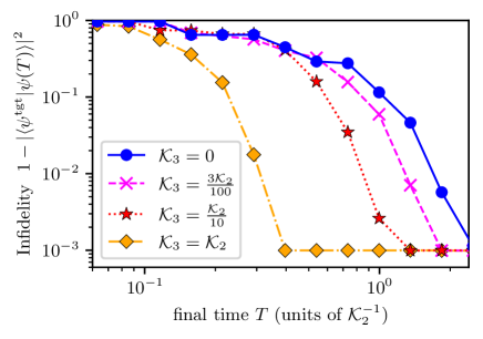
Figure 1: Infidelity for different values of $\mathcal{K}_{3}$ after optimization plotted against pulse duration $T$. The different values of $\mathcal{K}_{3}$ are indicated by the marker style and color. All markers correspond to the smallest infidelity obtained from a series of optimizations performed with the same parameters but different guess pulses.

So far, the accelerated preparation of the cat states through nonlinearities has relied on the assumption of coherent states as initial states. But, in practice, it is more feasible to start from the vacuum state. This suggests that a straightforward protocol for creating these states from the vacuum state can constist of generating a coherent state via the application of a short, coherent Gaussian pulse of appropriate strength and afterwards allowing the system to evolve without any additional drive. However, this raises the question of whether these field-free dynamics indeed yield the shortest realization of the cat state preparation or if taylored pulses can achieve even faster implementations, harvesting the full potential of the additional anharmonicities. Quantum optimal control [15, 16] allows us to answer this particular question and estimate the fundamental limit of how fast cat states can be generated by utilizing higher-order nonlinearities. In particular, we investigate how adding a linear drive

$$\hat{H}_{i} =\varepsilon(t)(\hat{a}+\hat{a}^{\dagger})\,,$$ (5)

with an appropriately shaped pulse $\varepsilon(t)$, to the Hamiltonian in Eq. 1 can further speed up the generation of a cat state.

For the optimization, we employ Krotov’s method [17, 18, 19] to minimize the infidelity $1-\big{|}\langle\psi_{\mathrm{cat}}|\psi(T)\rangle\big{|}^{2}$, which we use as optimization functional. This corresponds to maximizing the overlap between the evolved state $|\psi(T)\rangle$ at final time $T$ and the target cat state $|\psi_{\mathrm{cat}}\rangle$ from Eq. 3. The quantity to be optimized is the pulse shape of the linear drive. Using this, the shortest possible pulse duration is determined by optimizing towards the same cat state for different pulse durations $T$. Similar protocols have proven to be capable of identifying the shortest possible pulse durations for various states and systems [20]. Each of the optimizations uses the ground state as the initial state. The pulse amplitude is restricted to $|\varepsilon(t)|\leq 30\mathcal{K}_{2}$ during all times. Similar optimizations with $|\varepsilon(t)|\leq 5\mathcal{K}_{2}$, did not yield a significant speedup for larger nonlinearities.

Fig. 1 shows the optimization results for different values of $\mathcal{K}_{3}$, which varies between the different curves. All curves exhibit a similar shape, but are offset from one another. If the pulse duration is long enough, the optimization can reach very small infidelities, i.e. a large overlap between the final state and the targeted cat state. In Fig. 1 the smallest reached infidelity lies at $10^{-3}$, which corresponds to the fidelities for which the optimization was assumed to have converged. Reaching this value is assumed to be a successful preparation of the cat state. On the other hand, if the pulse duration is too small, it is not possible anymore to reach the target state, which is indicated by an increase of the final infidelities towards shorter pulse durations. The shortest pulse duration for which the optimization still succeeds is then considered to be the the physical bound for the preparation of the cat state. The curves in Fig. 1, show a clear shift towards shorter times for larger values of $\mathcal{K}_{3}$. The preparation time for $\mathcal{K}_{3}=0$ (solid blue curve) is longer compared to the one without linear drive, which corresponds to $T_{\mathrm{min}}=\frac{\pi}{2}\mathcal{K}_{2}$. This originates from the fact, that the optimization starts in the ground state. In contrast to this, the shortest possible pulse duration decreases by about a factor of 5 for the case when $\mathcal{K}_{3}=\mathcal{K}_{2}$. This demonstrates that higher-order terms can indeed be utilized for reducing the preparation time for cat states.

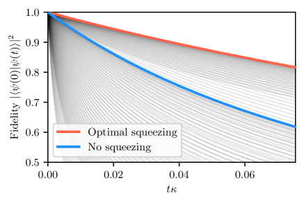
Figure 2: Overlap decay curves comparing the optimized squeezed cat states with other squeezed cat states. The curves show the pure decay of the system under dissipation, i.e. without Kerr nonlinearities and free oscillations. Besides the optimized squeezed cat state (in red) and the unsqueezed cat state (in blue), we also show curves for other squeezing parameters $r$ (from 0 to 1) and $\phi=0,\text{ }\frac{\pi}{2}\text{ and }\pi$ (in light blue). The cat state amplitude is set to be $\alpha=2$ for illustration, and $\kappa_{1\mathrm{ph}}=\kappa_{\phi}$ (only for illustration purpose, not specified to a physical platform), for which we find the optimized squeezing parameters to be $\phi=0$ and $r\approx 0.51$. The red curve illustrates the result with $\phi=0$ and $r\approx 0.51$.

In practice, the impact of dissipation will accumulate in time and decohere quantum states. Although it can be ignored in the quick cat preparation stage discussed previously (see supplementary materials), it has to be considered when dealing with larger timescales such as the storage of cat states in a noisy environment. It has been experimentally and numerically shown, that squeezing cat states makes them more robust under the two major types of dissipation: 1-photon loss and dephasing, prolonging the lifetime of cat states [14, 13]. Here, we squeeze cat states with the operator $\hat{S}(r,\phi)=e^{\frac{1}{2}r(e^{-i\phi}\hat{a}^{2}-e^{i\phi}\hat{a}^{{\dagger}2})}$, and analytically derive an optimal condition for the squeezing parameter $r$ and phase $\phi$ to reach the maximum protection.

To determine the benefits gained from squeezing cat states, we model dissipation and dephasing with the Lindblad equation, and look at their effects on an initially ideal squeezed cat state $|\psi_{\mathrm{SqCat}}\rangle$. While the state evolves under dissipation, we compute and expand the overlap $\mathcal{V}=|\langle\psi_{\mathrm{SqCat}}|\psi_{\mathrm{sys}}\rangle|^{2}$ between the system state $|\psi_{\mathrm{sys}}\rangle$ and the target state $|\psi_{\mathrm{SqCat}}\rangle$ (see supplementary material):

$$\mathcal{V} \approx 1-\kappa_{1\mathrm{ph}}K^{(1)}-\kappa_{\phi}K^{(2)}+\frac{\kappa_{1\mathrm{ph}}\kappa_{\phi}}{2}\left(K^{(3)}+2K^{(1)}K^{(2)}\right)$$

$$\hskip 14.22636pt+\mathcal{O}(\kappa_{1\mathrm{ph}}^{2},\kappa_{\phi}^{2})$$ (6)

where $t\kappa_{1\mathrm{ph}}\rightarrow\kappa_{1\mathrm{ph}}$ and $t\kappa_{\phi}\rightarrow\kappa_{\phi}$ are dimensionless rates of 1-photon loss and dephasing rescaled with time, $K^{(n)}$ is the n-th cumulant of $\hat{a}^{\dagger}\hat{a}$ with respect to the target state, e.g. $K^{(1)}=\langle\hat{a}^{\dagger}\hat{a}\rangle$, and $K^{(2)}=\langle(\hat{a}^{\dagger}\hat{a})^{2}\rangle-\langle\hat{a}^{\dagger}\hat{a}\rangle^{2}$. $\mathcal{O}(\kappa_{1\mathrm{ph}}^{2},\kappa_{\phi}^{2})$ corresponds to the expansions in $\kappa_{1\mathrm{ph}}^{2}$, $\kappa_{\phi}^{2}$ that are irrelevant here, as well as higher-orders that are ignored for weak enough decays.

The terms linear in $\kappa_{1\mathrm{ph}}$ and $\kappa_{\phi}$ from Eq. (6) indicate that in the presence of only 1-photon loss or dephasing, the optimal squeezing for maximally protecting cat states occurs in such a way that the average photon number $\langle\hat{a}^{\dagger}\hat{a}\rangle$ or the photon number variance $\sigma_{N}^{2}=K^{(2)}$ in the system is minimized. In the presence of both types of dissipation, a compromise between these quantities must be made. This can be done by tuning the squeezing parameter $r$ and its phase $\phi$ to a particular value, which has been calculated in supplementary material. We stress that the choice of $r$ and $\phi$ depends on the coherent state amplitude $|\alpha|$ in cat states, as well as the number of cat state components. In addition, the cross term $\kappa_{1\mathrm{ph}}\kappa_{\phi}$ suggests that 1-photon loss and dephasing can enhance the influence of each other, leading to the “loss-dephasing” phenomenon [21], and may play a significant role at later time when $\kappa_{1\mathrm{ph}}$ and $\kappa_{\phi}$ become large. To visualize our discussion, in Fig. 2, we plot how the overlap $\mathcal{V}$ (or fidelity) decays over the dimensionless time $t\kappa=\kappa_{1\mathrm{ph}}=\kappa_{\phi}$ for different values of $r$ and $\phi$. The slowest decay occurs at the point where the average and varaince of the photon number have made a good compromise, see supplementary material.

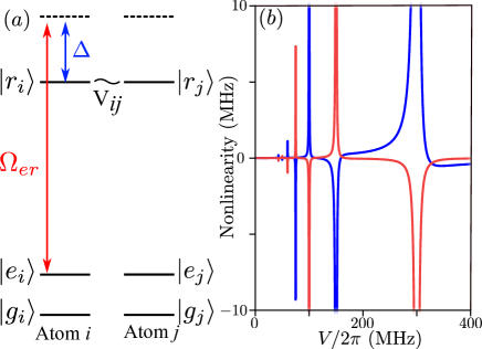
Figure 3: (a): Energy level structures of two Rydberg atoms interacting via Rydberg interaction. $g$, $e$ and $r$ denote ground state, excited state and Rydberg state. A laser of Rabi frequency $\Omega_{er}$ drives the transition $e\leftrightarrow r$ transitions with a detuning $\Delta$. Two Rydberg states $|r_{i}\rangle$ and $|r_{j}\rangle$ interact via $V_{ij}$. (b): Nonlinear strengths $\mathcal{K}_{2}$ and $\mathcal{K}_{3}$ of second (blue) and third (red) orders in units of the linear frequency $\mathcal{K}_{1}$, plotted from the effective Hamiltonian Eq. (7) using $\Omega_{er}/2\pi=50\text{ MHz}$, $\Delta/2\pi=150\text{ MHz}$. Both orders of nonlinearity grow stronger near the multiphoton resonance regions, where $V=\frac{2\Delta}{m}$ for $m=1,2,3,...$.

We now consider the prospects for using higher-order nonlinearities to speed up cat-state preparation in experiments. While these nonlinearities at the required strength are difficult to create in e.g. superconducting systems [22], Rydberg atoms, which exhibit a wide range of applications [23, 24, 25], can provide a suitable alternative. We consider an ensemble of Rydberg atoms where each atom has three energy levels (ground $|g\rangle$, excited $|e\rangle$ and Rydberg $|r\rangle$ states). Two atoms namely i and j interact with each other via $V_{ij}$ if both are in Rydberg states, see Fig. 3 (a). The transition between excited and Rydberg states of each atom is driven at the Rabi frequency $\Omega_{er}$ with a detuning $\Delta$. In the limit of $\Delta>>\Omega_{er}$, we can adiabatically eliminate the Rydberg states from the system due to their short lifetime $\sim\frac{1}{\Delta}$, so that there are only ground and excited states left. In other words, since atoms in Rydberg states quickly decay to excited states, we may regard them as if they have always been in excited states. The effective Hamiltonian after eliminating the Rydberg states is (see supplementary material)

$$\hat{H}_{eff} =\sum_{n=2}^{N}\mathcal{K}_{n}\hat{N}_{e}^{n},$$ (7)

where $\mathcal{K}_{n}=\sum_{m=0}^{N-1}s(m+1,n)f(m)$ for which $s(m,n)$ is the Stirling number of the first kind and

$$f(m) =\begin{cases}\frac{\Omega_{er}^{2}}{4\Delta}&m=0,\\ \frac{1}{(m-1)!}\frac{V\Omega_{er}^{2+2m}}{2^{3+2m}\Delta(\Delta-\frac{m}{2}V)\prod_{k=1}^{m}(\Delta-\frac{k-1}{2}V)^{2}}\hskip 14.22636pt&\text{else}.\end{cases}$$

$\hat{N}_{e}=\sum_{i=1}^{N}\hat{\sigma}_{i}^{ee}$ is the number operator that is generated from the atomic operator $\hat{\sigma}_{i}^{ee}$ acting on the ith atom, this operator counts how many excited states are in the system. We note that Eq. (7) is of the same form as Eq. (1). Nonlinear coefficients may diverge due to singularities that come from the denominator of $f(m)$, and correspond to $m+1$-photon resonances. In other words, we may obtain strong nonlinearities by tuning the system to regions near these singularities. As an illustration, $\mathcal{K}_{2}$ and $\mathcal{K}_{3}$ have been plotted in units of the linear frequency $\mathcal{K}_{1}$ (see Fig. 3 (b)), and they diverge at $V=\frac{2\Delta}{m}$ for $m=1,2,3,...$, which correspond to the $m+1$-photon resonance, or the Rydberg blockade [26, 27, 28]. We can treat Eq. (7) as a bosonized version of an atomic ensemble, in which Fock state represents the number of excited states in the ensemble, and the coherent state follows the binomial distribution which agrees with the Poisson distribution when the ensemble contains large enough number of atoms. Such atomic coherent states have been well studied in two-level system ensembles [29, 30, 31, 32].

To create the initial (atomic) coherent state required from the cat preparation scheme, we need to add another laser that drives the transition between ground and excited states of each atom:

$$\hat{H}_{eff}^{\prime} =\sum_{i=2}^{N}\mathcal{K}_{i}(\hat{a}^{\dagger}\hat{a})^{i}\otimes\mathds{1}+\frac{\Omega_{eg}}{2}(e^{i(\mathcal{K}_{1}+\omega_{eg})t}\hat{a}^{\dagger}\otimes\hat{a}+\mathrm{h.c.}),$$ (8)

where $\Omega_{eg}$ is the frequency of the laser, $\omega_{eg}$ is the energy difference between ground and excited states, and $\mathcal{K}_{1}$ is the linear term coefficient. The system state is denoted as $|N_{e}\rangle\otimes|N_{g}\rangle$ corresponding to the two modes in Eq. (8): the first mode denotes the number of atoms in excited state, and the second in ground state.

We now look at some experimental aspects. We first want to maintain a certain distance from the multiphoton resonance regions; although we obtain strong nonlinearities near these regions, our assumptions of adiabatic elimination may also break down, causing the accuracy of the effective Hamiltonian to drop. We analyzed several regions using realistic experimental parameters [28, 33, 34, 35, 11], e.g. $\Omega_{er}/2\pi=50\text{ MHz}$, $-200\leq\Delta/2\pi\leq 200\text{ MHz}$, and $-400\leq V/2\pi\leq 400\text{ MHz}$, and found that there are regions where we can obtain strong higher-order nonlinearities, while the effective Hamiltonian in Eq. (7) still holds accurate. The detailed discussions are provided in supplementary material. In these regions, preparation times of the cat state are of three orders of magnitude shorter than its lifetime derived from [36].

To conclude, cat states can be quickly generated by a proper tuning of multiple higher order nonlinear coefficients in an anharmonic system, such that the shortest limit of cat preparation time depends on the maximum anharmonic order. In addition to this, employing a controllable coherent driving to the system further accelerates the cat generation process, pushing the preparation time beyond the previous limit. After being prepared, cat states can also survive longer in a noisy environment with an appropriate squeezing. Moreover, an ensemble of Rydberg atoms can be used to implement the cat preparation scheme, but has the experimental challenge of maintaining constant nonlinearities.

We acknowledge fruitful discussions with F. Gago Encinas, L. Orr, and N. Diaz-Naufal. AM acknowledges funding by the Deutsche Forschungsgemeinschaft through the Emmy Noether program (Grant No. ME 4863/1-1) and the project CRC 183. SQ is funded in part by the Wallenberg Initiative on Networks and Quantum Information (WINQ) and in part by the Marie Skłodowska–Curie Action IF programme “Nonlinear optomechanics for verification, utility, and sensing” (NOVUS) – Grant-Number 101027183. Nordita is partially supported by Nordforsk. MGK and CPK acknowledge financial support from the Deutsche Forschungsgemeinschaft (DFG), Project No. 277101999, CRC 183 (project C05).

Supplementary material

Nonlinear parameters

In this appendix, we derive Eq. (4) and demonstrate how we calculate nonlinear parameters $\mathcal{K}_{i\geq 2}$ in Eq. (2), so that with these parameters, a coherent state may evolve into the cat state

$$|\psi_{\mathrm{cat}}\rangle =\frac{1-i}{2}|\alpha\rangle+\frac{1+i}{2}|-\alpha\rangle,$$ (9)

that is a cat state of $\phi=\frac{\pi}{2}$, where $\phi$ is the phase characterizing a particular cat state. The evolution of the coherent state under nonlinearity has been visualized in Fig. 4.

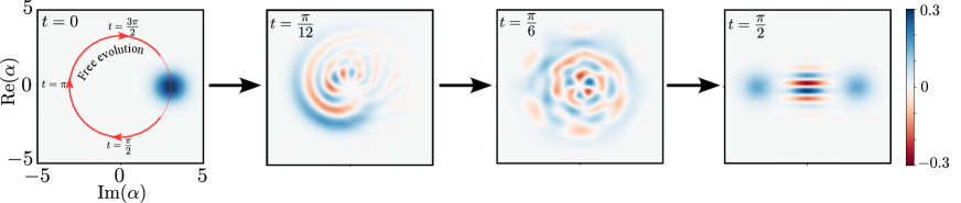
Figure 4: Wigner function plots of a coherent state evolving into a cat state under the nonlinearities. Without nonlinearity, the initial coherent state (the blue spot in the upper-left figure) would only rotate along the red circular path, which can be removed by going to a rotating frame about the free evolution. With nonlinearity, which we chose the self-Kerr interaction $\hat{H}=(\hat{a}^{\dagger}\hat{a})^{2}$ for simplicity, the initial coherent state would be smeared during its evolution, and eventually turn into a cat state. Here, we show two intermediate steps at $t=\frac{\pi}{12}$ and $t=\frac{\pi}{6}$ to visualize how the coherent state gets smeared out. At $t=\frac{\pi}{2}$, the smearing accumulates to the extent such that two blue spots appears with several strips in between, and is called a cat state.

The key requirement for a coherent state to evolve into the cat state is to make the time evolution $e^{-ip(n)t_{c}}$ dependent only on the parity of number eigenstates at the time $t_{c}$, so that each parity corresponds to a cat component ($|\alpha\rangle$ and $|-\alpha\rangle$ in our case). In other words, if we take a factor of $\pi$ out of time such that $t_{c}=\pi t_{c}^{\prime}$ for convenience, then we would want to find the product $p(n)t_{c}^{\prime}$ such that:

$$p(n)t_{c}^{\prime}=\begin{cases}0\ (\mathrm{mod}\ 2)\hskip 56.9055pt&n=\mathrm{even},\\ \frac{1}{2}\ (\mathrm{mod}\ 2)&n=\mathrm{odd},\end{cases}$$ (10)

which produces the correct phase for the two cat components. Here, we use the modulus notation $a\ (\mathrm{mod}\ 2)=a+2z$ where $z$ can be any integers, because phase factors with a difference of $2z\pi$ give rise to the same result.

To simplify our calculations later, we first rewrite $p(n)$ in another basis, the so-called binomial basis:

$$p(n) =\sum_{j=2}^{m}\mathcal{K}_{j}n^{j}=\sum_{r=1}^{m}a_{r}\binom{n}{r},$$ (11)

where $\mathcal{K}_{j}$ are coefficients of the j-th order nonlinearity shown in Eq. (1), $a_{r}$ are coefficients of our new binomial basis, e.g., $\binom{n}{2}=\frac{n(n-1)}{2!}$. The transformation between coefficients of the usual polynomial basis $n^{j}$ and the binomial basis $\binom{n}{r}$ can be done via:

$$\mathcal{K}_{j} =\sum_{r=1}^{m}\frac{s(r,j)}{r!}a_{r},$$ (12)

where $s(r,j)$ is Stirling number of the first kind.

Denoting $a_{r}t_{c}^{\prime}=\gamma_{r}$, we can insert $n=1,2,...,m$ into the $p(n)$ in Eq. (10), and obtain $m$ equations about $\gamma_{1,2,...,m}$, which can be solved when using the binomial basis for $p(n)$:

$$\gamma_{1} =\frac{1}{2}\ (\mathrm{mod}\ 2),$$

$$2\gamma_{1}+\gamma_{2} =0\ (\mathrm{mod}\ 2),$$

$$3\gamma_{1}+3\gamma_{2}+\gamma_{3} =\frac{1}{2}\ (\mathrm{mod}\ 2),$$

$$...,$$

$$\sum_{j=1}^{m}\gamma_{j}\binom{m}{j} =\begin{cases}0\ (\mathrm{mod}\ 2)\hskip 14.22636ptm=\mathrm{even},\\ \frac{1}{2}\ (\mathrm{mod}\ 2)\hskip 14.22636ptm=\mathrm{odd},\end{cases}$$

where the first equation tells $\gamma_{1}=\frac{1}{2}\ (\mathrm{mod}\ 2)$, which then implies that the second equation tells $\gamma_{2}=1\ (\mathrm{mod}\ 2)$, similarly the third equation tells $\gamma_{3}=0\ (\mathrm{mod}\ 2)$, and so on. In general, we have $\gamma_{3}=\gamma_{4}=...=\gamma_{m}=0\ (\mathrm{mod}\ 2)$.

After finding all $\gamma_{j=1,2,...,m}$, we can choose, without loss of generality, $\mathcal{K}_{m}=1$ to rescale our unit system such that $\frac{\mathcal{K}_{j<m}}{\mathcal{K}_{m}}\rightarrow\mathcal{K}_{j<m}$ and time $t\mathcal{K}_{m}\rightarrow t$ become dimensionless. This corresponds to choose a specific timescale of the Hamiltonian, in which we can rewrite $\mathcal{K}_{m}t_{c}^{\prime}=1t_{c}^{\prime}$ using Eq. (12):

$$\sum_{r=1}^{m}\frac{s(r,m)}{r!}\gamma_{r} =\frac{\gamma_{m}}{m!}=t_{c}^{\prime}.$$ (13)

Since $\gamma_{r}$ in Eq. (13) has been calculated in the modulus form which has infinitely many possible values, we want to find the specific values for $\gamma_{r}$ such that the time $t_{c}^{\prime}$ in Eq. (13) is the shortest possible time. We found that $t_{c}^{\prime}=\frac{\min\{1\ (\mathrm{mod}\ 2)\}}{2}=\frac{1}{2}$ for $m=2$, and $t_{c}^{\prime}=\frac{\min\{0\ (\mathrm{mod}\ 2)\}}{m!}=\frac{2}{m!}$ for $m>2$. Thus, we find the shortest possible time $t_{c,\mathrm{min}}$ taken by a coherent state to evolve into the cat state under Eq. (1) to be:

$$t_{c,\mathrm{min}}=\begin{cases}\frac{\pi}{2\mathcal{K}_{2}}&\text{ for $m=2$},\\ \frac{2\pi}{\mathcal{K}_{m}m!}&\text{ for $m>2$}.\end{cases}$$ (14)

To calculate other $\mathcal{K}_{n<m}$, we first note that Eq. (13) only imposes a constraint to $\gamma_{m}$, which indirectly suggests that we are free to take any values for other $\gamma_{1,2,...,m-1}$. In other words, we can choose any values for $\gamma_{1,2,...,m-1}$ that satisfy their modulus condition, e.g., $\gamma_{3}=2,4,6=0\ (\mathrm{mod}\ 2)$. However, in practice, we always have constraints, such as lower order nonlinearities sometimes can be either stronger, weaker, or equal to the m-th order nonlinearity. Hence, we will need to solve the system consisting of Eq. (13) and:

$$|\mathcal{K}_{k<m}|t_{c}^{\prime} \sim|\mathcal{K}_{m}|t_{c}^{\prime}=t_{c}^{\prime}$$

$$\left|\sum_{k=1}^{m}\frac{s(k,n)}{k!}\gamma_{k}\right| \sim t_{c}^{\prime},$$ (15)

where $\sim$ indicates possible constraints on lower order nonlinear strengths $\mathcal{K}_{n<m}$, e.g., $\sim=\leq$ indicates $|\mathcal{K}_{k<m}|\leq|\mathcal{K}_{m}|$ for some $n$.

Master equation analysis

We have shown that cat states can be prepared in a very short time, during which the influence of noise may be neglected. In this appendix, we assume that we start with a perfect cat state and have turned off the nonlinearities in the system such that its Hamiltonian is $\hat{H}=0$ in the rotating frame about the free Hamiltonian. As discussed in the main text, it has been previously shown experimentally and numerically that squeezing the cat-state protects it from noise [14, 13]. Here, we take a closer look at how squeezing the cat state would protect it from noise (namely 1-photon loss and dephasing), and derive an optimal condition to maximize the protection from squeezing. We achieve this by analytically solving the Lindblad equation for 1-photon loss and dephasing.

We first show that 1-photon loss and dephasing induce an $\mathfrak{su}(1,1)$ algebra by extending the results in [37], and hence the vectorized Lindblad equation reads [38, 39, 40]

$$\frac{d}{dt}|\hat{\rho}(t)\rrangle =\left(-\frac{\kappa_{1\mathrm{ph}}}{2}\hat{K}_{3}-\frac{\kappa_{\phi}}{2}\hat{K}_{0}^{2}+\kappa_{1\mathrm{ph}}\hat{K}_{-}\right)|\hat{\rho}(t)\rrangle,$$ (16)

where $\kappa_{1\mathrm{ph}}$ and $\kappa_{\phi}$ are 1-photon loss and dephasing respectively, and

$$\hat{K}_{-} =\hat{a}\otimes\hat{a},$$

$$\hat{K}_{0} =\hat{a}^{\dagger}\hat{a}\otimes\mathds{1}-\mathds{1}\otimes\hat{a}^{\dagger}\hat{a},$$

$$\hat{K}_{3} =\hat{a}^{\dagger}\hat{a}\otimes\mathds{1}+\mathds{1}\otimes\hat{a}^{\dagger}\hat{a}.$$ (17)

Here, we have grouped different terms in the Lindblad equation to emphasize its $\mathfrak{su}(1,1)$ structure that is usually denoted as $\mathfrak{su}(1,1)=\{\hat{K}_{0},\hat{K}_{3},\hat{K}_{+},\hat{K}_{-}\}$. In our case, $\hat{K}_{+}=\hat{a}^{\dagger}\otimes\hat{a}^{\dagger}$ would correspond to a thermalized environment that also pumps thermal photons to the system. For simplicity, we choose to use the Lindblad equation that assumes a “cold” environment with no thermal photons $\bar{n}=0$, (e.g., an optical system which has its stationary state being the vacuum state, or a superconducting system which is cooled to nearly 0K), but one can still proceed similarly as the followings to obtain a similar solution for the master equation with $\bar{n}\neq 0$.

We note the ansatz that the exact solution to Eq. (16) is

$$|\hat{\rho}(t)\rrangle =\hat{\mathcal{S}}(t)|\hat{\rho}(0)\rrangle,$$ (18)

where $\hat{\mathcal{S}}(t)=e^{F_{0}(t)\hat{K}_{0}^{2}}e^{F_{3}(t)\hat{K}_{3}}e^{F_{-}(t)\hat{K}_{-}}$, with $F_{0}$, $F_{3}$ and $F_{-}$ time dependent functions. We calculate $F_{0}$, $F_{3}$ and $F_{-}$ by evaluating $\left(\frac{d}{dt}\hat{\mathcal{S}}(t)\right)\hat{\mathcal{S}}^{-1}(t)$: we can either insert Eq. (18) back to Eq. (16), or work directly with the expression of $\hat{\mathcal{S}}(t)$ from Eq. (18). If we equate the results from both ways, we obtain

$$-\frac{\kappa_{1\mathrm{ph}}}{2}\hat{K}_{3}+\kappa_{1\mathrm{ph}}\hat{K}_{-} =\dot{F}_{3}(t)\hat{K}_{3}+\dot{F}_{-}(t)e^{-2F_{3}(t)}\hat{K}_{-},$$ (19)

where we have made use of the fact that $\hat{K}_{0}$ is the Casimir element which commutes with all other operators, so that we can take its term out:

$$F_{0}(t)=-\frac{\kappa_{\phi}}{2}t.$$ (20)

Equating the coefficients for $\hat{K}_{3}$ and $\hat{K}_{-}$, we obtain

$$F_{3}(t) =-\frac{\kappa_{1\mathrm{ph}}}{2}t,$$

$$F_{-}(t) =1-e^{-\kappa_{1\mathrm{ph}}t}.$$ (21)

Put all these together, we get

$$\hat{\mathcal{S}}(t) =e^{-\frac{\kappa_{\phi}}{2}\hat{K}_{0}^{2}t}e^{-\frac{\kappa_{1\mathrm{ph}}}{2}\hat{K}_{3}t}e^{(1-e^{-\kappa_{1\mathrm{ph}}t})\hat{K}_{-}}.$$ (22)

To determine the impact of noises during a time period $t$, we use the notion of overlap. The overlap between the squeezed state in the system and the target squeezed cat state is

$$\mathcal{V}(t) =\llangle\psi_{\mathrm{cat}}|\hat{S}^{-1}(r,\phi)\hat{\mathcal{S}}(t)\hat{S}(r,\phi)|\psi_{\mathrm{cat}}\rrangle,$$ (23)

where $\hat{S}(r,\phi)=e^{\frac{1}{2}r(e^{-i\phi}\hat{a}^{2}-e^{i\phi}\hat{a}^{{\dagger}2})}$ is the squeezing operator with the squeezing strength $r$ and phase $\phi$.

For small $\kappa_{1\mathrm{ph}}t$ and $\kappa_{\phi}t$, we can expand Eq. (22) up to the second order about $\kappa_{1\mathrm{ph},\phi}$ and evaluate the overlap:

$$\mathcal{V}(t) \approx 1-\kappa_{1\mathrm{ph}}\langle\hat{N}\rangle-\kappa_{\phi}(\langle\hat{N}^{2}\rangle-\langle\hat{N}\rangle^{2})$$

$$\hskip 5.69046pt+\frac{\kappa_{1\mathrm{ph}}^{2}}{4}\left(\langle\hat{N}^{2}\rangle+\langle\hat{N}\rangle^{2}+2|\langle\hat{a}^{2}\rangle|^{2}\right)$$

$$\hskip 5.69046pt+\frac{\kappa_{\phi}^{2}}{4}\left(\langle\hat{N}^{4}\rangle+3\langle\hat{N}^{2}\rangle^{2}-4\langle\hat{N}^{3}\rangle\langle\hat{N}\rangle\right)$$

$$\hskip 5.69046pt+\frac{\kappa_{1\mathrm{ph}}\kappa_{\phi}}{2}\left(\langle\hat{N}^{3}\rangle-\langle\hat{N}\rangle\langle\hat{N}^{2}\rangle\right),$$ (24)

where $\hat{N}=\hat{a}^{\dagger}\hat{a}$, and $\langle\hskip 2.84544pt\bullet\hskip 2.84544pt\rangle$ is the expectation value with respect to the squeezed cat state. In general, we note that any type of decay of the form $\sqrt{\kappa_{D}}\hat{D}$ would contribute a linear term $-\kappa_{D}(\langle\hat{D}^{\dagger}\hat{D}\rangle-\langle\hat{D}\rangle^{2})$ to the expression of $\mathcal{V}(t)$.

Adiabatic elimination

In this appendix, we consider a collection of identical Rydberg atoms with the atomic energy levels shown in Fig. 3 (a), and show that such an atomic ensemble exhibit nonlinearities in Eq. (1). As shown in Fig. 3 (a), each atom has three energy levels: ground $|g\rangle$, excited $|e\rangle$ and Rydberg states $|r\rangle$, and two atoms $i$ and $j$ interact with each other via $V_{ij}$ when both are in Rydberg states $|r_{i}\rangle\otimes|r_{j}\rangle$. The intuition for the presence of nonlinearities lies in the fact that the energy $E$ of the ensemble does not depend linearly on the number of atoms in Rydberg states $k$, but $E\propto\frac{k^{2}-k}{2}V_{ij}$. The nonlinear dependence gets even more complicated in terms of the number of atoms in excited states, due to the laser that drives the transition between excited and Rydberg states. Here, we derive an expression of the nonlinear Hamiltonian by adiabatically eliminating Rydberg states from the ensemble, and show the nonlinearity of the system in the number of atoms in excited states.

We start from the raw Hamiltonian of the ensemble containing N atoms

$$\hat{H}_{\mathrm{raw}} =\frac{\Omega_{er}}{2}\sum_{i=1}^{N}(\hat{\sigma}_{i}^{re}+\hat{\sigma}_{i}^{er})-\Delta\hat{\sigma}_{i}^{rr}+\frac{V}{2}\sum_{j\neq i}^{N}\hat{\sigma}_{i}^{rr}\hat{\sigma}_{j}^{rr}.$$ (25)

where $\Omega_{er}$ is the Rabi frequency of the laser driving the transition between excited and Rydberg states and $\Delta$ is the detuning of the laser, $\hat{\sigma}_{i}^{xy}=|x\rangle\langle y|$ are jump operators for the i-th atom, and we assume a constant Rydberg interaction $V_{ij}=V$. The Schrödinger equation for only the $i$-th atom being at the Rydberg state $|r_{i}\rangle$ is

$$i\frac{d}{dt}|r_{i}\rangle =\frac{\Omega_{er}}{2}|e_{i}\rangle-\left(\Delta-\frac{(N_{r}-1)}{2}V\right)|r_{i}\rangle,$$ (26)

where $N_{r}$ denotes the number of Rydberg states.

The assumption of adiabatic elimination $|\Delta|>>\Omega_{er}$ enters as we equate Eq. (26) to zero, which is similar to the elimination of the fast oscillating mode from the system:

$$|r_{i}\rangle =\frac{\Omega_{er}}{2\left(\Delta-\frac{(N_{r}-1)}{2}V\right)}|e_{i}\rangle.$$ (27)

Now, we need to consider case by case. The first case is that the system has no atoms at Rydberg states, in which we can write the Schrödinger equation for the i-th atom being at the excited state as

$$i\frac{d}{dt}|e_{i}\rangle =\frac{\Omega_{er}}{2}|r_{i}\rangle\stackrel{{\scriptstyle\mathrm{Eq.}\eqref{Eq16}}}{{=}}\frac{\Omega_{er}^{2}}{4\Delta}|e_{i}\rangle,$$ (28)

and obtain the single-body Hamiltonian

$$\hat{H}_{eff}^{1}=\frac{\Omega_{er}^{2}}{4\Delta}\sum_{i}^{N}\hat{\sigma}_{i}^{ee}=\frac{\Omega_{er}^{2}}{4\Delta}\hat{N}_{e},$$ (29)

where $\hat{N}_{e}=\sum_{i}^{N}\hat{\sigma}_{i}^{ee}$ denotes the number operator counting the number of excited states.

Similarly, the second case is that the system has one Rydberg state, then

$$i\frac{d}{dt}|e_{i},r_{j}\rangle-i\left(\frac{d}{dt}|e_{i}\rangle\right)\otimes|r_{j}\rangle=\bigg{[}\frac{\Omega_{er}^{3}}{8\Delta(\Delta-\frac{V}{2})}-\frac{\Omega_{er}^{3}}{8\Delta^{2}}\bigg{]}|e_{i},e_{j}\rangle,$$ (30)

where we subtract the single body terms from the two body term to obtain the pure two body interaction. The Hamiltonian corresponding to the two body interaction is

$$\hat{H}_{eff}^{2} =\bigg{(}\frac{\Omega_{er}^{3}}{8\Delta(\Delta-\frac{V}{2})}-\frac{\Omega_{er}^{3}}{8\Delta^{2}}\bigg{)}\sum_{\begin{subarray}{c}i,j\\ i\neq j\end{subarray}}\hat{\sigma}_{i}^{ee}\hat{\sigma}_{j}^{er},$$ (31)

but $\hat{\sigma}^{er}=|e\rangle\langle r|=\frac{\Omega_{er}}{2\Delta}|e\rangle\langle e|=\frac{\Omega_{er}}{2\Delta}\hat{\sigma}^{ee}$, so we eventually have

$$\hat{H}_{eff}^{2} =\frac{\Omega_{er}}{2\Delta}\bigg{(}\frac{\Omega_{er}^{3}}{8\Delta(\Delta-\frac{V}{2})}-\frac{\Omega_{er}^{3}}{8\Delta^{2}}\bigg{)}\binom{\hat{N}_{e}}{2},$$ (32)

where $\binom{\hat{N}_{e}}{2}$ denotes the binomial representation of $\frac{\hat{N}_{e}(\hat{N}_{e}-1)}{2}$.

We can obtain $\hat{H}_{eff}^{j>2}$ by proceeding similarly for other cases in which there are two or more Rydberg states in the ensemble. Summing up all the Hamiltonians $\hat{H}_{eff}^{j}$, we have

$$\hat{H}_{eff} =\sum_{i=1}^{N}\hat{H}_{eff}^{i},$$

$$=\sum_{n=1}^{N}\underbrace{\left(\sum_{m=0}^{N-1}s(m+1,n)f(m)\right)}_{\mathcal{K}_{n}}\hat{N}_{e}^{n}=\sum_{n=1}^{N}\mathcal{K}_{n}\hat{N}_{e}^{n},$$ (33)

where $s(m,n)$ is the Stirling number of the first kind, and

$$f(m) =\begin{cases}\frac{\Omega_{er}^{2}}{4\Delta}&m=0,\\ \frac{1}{(m-1)!}\frac{V\Omega_{er}^{2+2m}}{2^{3+2m}\Delta(\Delta-\frac{m}{2}V)\prod_{k=1}^{m}(\Delta-\frac{k-1}{2}V)^{2}}\hskip 14.22636pt&\text{else}.\end{cases}$$ (34)

For example, the strength of $\mathcal{K}_{2}$ is plotted in Fig. 5. Similar plots apply for $\mathcal{K}_{i\geq 3}$. As shown in the figure, stronger nonlinearities occur near the multiphoton resonance regions, where the assumptions for adiabatic elimination break down and the effective Hamiltonian loses its accuracy. We therefore want to examine several regions to show that we can obtain stronger higher order nonlinearities while the effective Hamiltonian remains accurate, and results are given in Table. 1.

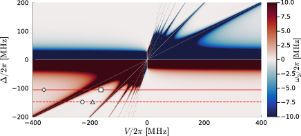
Figure 5: Strenght of $\mathcal{K}_{2}$ for varying $\Delta$ and $V$. The horizontal band around $\Delta=0$ corresponds to the single photon resonance. One could find large second order nonlinearites here, but it is also where the approximation $|\Delta|>>\Omega_{er}$ breaks down and where we expect large losses from the high r state admixture. The upper left and lower right quadrants (away from $\Delta\sim 0$) represent relatively ”stable” regions but with correspondingly weak nonlinearities. The (strong) Rydberg blockade condition is expected for $|V|>>|\Delta|,\text{ }\Omega_{er}$ (far left or right of graph). Radiating ”rays” from the center correspond to multiphoton resonances where $\mathcal{K}_{2}$ diverges, e.g., $\Delta-\frac{m}{2}V=0$ associated to the $m+1$-photon resonance. To minimize collective losses, one should also avoid these rays. But in between one can obtain relatively strong nonlinearities, including potentially interesting higher order nonlinearities ($\mathcal{K}_{3}$, $\mathcal{K}_{4}$, etc.).

Sym.	$\mathcal{K}_{2}[\mathrm{MHz}]$	$\mathcal{K}_{3}[\mathrm{MHz}]$	$\mathcal{K}_{4}[\mathrm{MHz}]$	$\tau[\mu s]$	$t_{c}[\mu s]$	$\epsilon$ [MHz]
-	0.34938	0	0	570.75	0.91	0.67451
$\blacksquare$	0.88096	0.02643	0.00001	496.27	0.22	2.90457
$\blacksquare$	0.63003	0.63002	0.02169	201.03	0.10	10.95341
$\blacktriangle$	0	0.08088	0.00343	374.15	0.6	0.90703
$\bullet$	-0.10195	0.10195	0.00194	299.04	0.6	1.09153

Table 1: Table for the selected points in Fig. 5, and an extra point out of the figure (labeled as $-$). The first three columns are strengths of nonlinearities $\mathcal{K}_{2}$, $\mathcal{K}_{3}$ and $\mathcal{K}_{4}$, $\tau$ is the lifetime calculated by considering the Rydberg decay rate $\gamma/2\pi=1.5\text{ kHz}$, $t_{c}$ is the preparation time of cat states obtained from the optimal control, and $\epsilon$ is the ground state energy difference per atom between the full Hamiltonian and the effective Hamiltonian, to quantify the error caused by the assumptions of adiabatic elimination.

Furthermore, We may also add a laser with Rabi frequency $\Omega_{eg}$ driving the transition between ground and excited states:

$$\hat{H}_{eff}^{\prime} =\hat{H}_{eff}+\frac{\Omega_{eg}}{2}\sum_{i}\left(\hat{\sigma}_{i}^{eg}+\hat{\sigma}_{i}^{ge}\right).$$ (35)

We define Fock states to be the number of excited atoms in symmetrized Dicke states [41]

$$|n\rangle =\{|g\rangle^{\otimes N-n}\otimes|e\rangle^{\otimes n}\}_{\mathrm{sym}},$$ (36)

then the atomic operators in Eq. (35) become

$$\sum_{i}\hat{\sigma}_{i}^{eg} =\hat{a}^{\dagger},$$

$$\sum_{i}\hat{\sigma}_{i}^{ge} =\hat{a},$$ (37)

such that

$$\hat{a}^{\dagger}|n\rangle =\sqrt{(n+1)(N-n-1)}|n+1\rangle,$$

$$\hat{a}|n\rangle =\sqrt{n(N-n+1)}|n-1\rangle.$$ (38)

This is atomic analogue of the coherent drive for $\mathfrak{su}(2)$ algebra (the creation and annihilation operators here have slightly different actions on Fock states to ensure the $SU(2)$ symmetry) to generate atomic coherent states, and we can make it controllable e.g., $\epsilon(t)\hat{a}+\epsilon^{*}(t)\hat{a}^{\dagger}$ to realize the full controllability of the system [41]. Note that in the main context, we instead use the notation $\hat{a}^{\dagger}\otimes\hat{a}$ with the usual definition of creation and annihilation operators to avoid confusion.

Optimized squeezing

Eq. (6) suggests that the optimal squeezing to maximally protect the cat state from 1-photon loss and dephasing occurs at around the minimum 1-st and 2-nd cumulants of the number operator $\hat{a}^{\dagger}\hat{a}$ respectively. Hence, it is sufficient to calculate $\langle\hat{a}^{\dagger}\hat{a}\rangle$ and $\langle(\hat{a}^{\dagger}\hat{a})^{2}\rangle$ with respect to the squeezed cat state $|\psi_{\mathrm{SqCat}}\rangle$ in this appendix, and the first two cumulants $K^{(1)}=\langle\hat{a}^{\dagger}\hat{a}\rangle$ and $K^{(2)}=\langle(\hat{a}^{\dagger}\hat{a})^{2}\rangle-\langle\hat{a}^{\dagger}\hat{a}\rangle$ can be minimized with mathematical softwares.

We first denote the squeezed c-component cat state that can be obtained in Yurke-Stoler’s method, with the fractional revival method, as [42]:

$$|\psi_{\mathrm{SqCat}}^{c}\rangle =\hat{S}(r,\phi)e^{\pm i\frac{\pi}{c}(\hat{a}^{\dagger}\hat{a})^{2}}|\alpha\rangle,$$ (39)

where $\hat{S}(r,\phi)=e^{\frac{1}{2}r(e^{-i\phi}\hat{a}^{2}-e^{i\phi}\hat{a}^{{\dagger}2})}$ is the squeezing operator.

Without loss of generality, we also assume $\alpha$ to be real. With this, we found

$$\langle\hat{a}^{\dagger}\hat{a}\rangle =\langle\psi_{\mathrm{SqCat}}^{c}|\hat{a}^{\dagger}\hat{a}|\psi_{\mathrm{SqCat}}^{c}\rangle,$$

$$=\sinh^{2}(r)+\alpha^{2}\cosh(2r)-\frac{1}{2}\sinh(2r)\alpha^{2}A,$$ (40)

and

$$\langle(\hat{a}^{\dagger}\hat{a})^{2}\rangle =\langle\psi_{\mathrm{SqCat}}^{c}|(\hat{a}^{\dagger}\hat{a})^{2}|\psi_{\mathrm{SqCat}}^{c}\rangle,$$

$$=\alpha^{2}(1+\alpha^{2})\cosh^{2}(2r)+\sinh^{4}(r)$$

$$\hskip 5.69046pt+2\alpha^{2}\sinh^{2}(r)\left(\cosh(2r)-\frac{1}{2}\sinh(2r)A\right)$$

$$\hskip 5.69046pt-\frac{1}{4}\sinh(4r)\alpha^{2}B+\frac{1}{4}\sinh^{2}(2r)C,$$ (41)

where

$$A =2e^{-\alpha^{2}}\text{Re}[e^{-i\phi}e^{i\frac{4\pi}{c}}e^{\alpha^{2}e^{i\frac{4\pi}{c}}}],$$

$$B =2e^{-\alpha^{2}}Re\bigg{[}e^{-i\phi}e^{i\frac{4\pi}{c}}e^{\alpha^{2}e^{i\frac{4\pi}{c}}}(\alpha^{2}+2+\alpha^{2}e^{i\frac{4\pi}{c}})\bigg{]},$$

$$C =2(\alpha^{2}+1)^{2}+2\alpha^{4}e^{-\alpha^{2}}Re\bigg{[}e^{-2i\phi}e^{i\frac{16\pi}{c}}e^{\alpha^{2}e^{i\frac{8\pi}{c}}}\bigg{]}.$$ (42)

$K^{(2)}$ or the photon number variance $\sigma_{N}^{2}$ of the system is then

$$\sigma_{N}^{2} =\langle(\hat{a}^{\dagger}\hat{a})^{2}\rangle-\langle\hat{a}^{\dagger}\hat{a}\rangle^{2},$$

$$=\alpha^{2}\cosh^{2}(2r)-\frac{1}{2}\cosh(2r)\sinh(2r)\alpha^{2}(B-2\alpha^{2}A)$$

$$\hskip 5.69046pt+\frac{1}{4}\sinh^{2}(2r)(C-\alpha^{4}A^{2}).$$ (43)

Note that for the 2-component cat state $c=2$, Eq. (40)-(42) are identical to that of the squeezed coherent states calculated in [43].

Finally, the optimal squeezing condition can be calculated by minimizing (40) and Eq. (42) with some mathematical softwares.

Controllability

In this appendix, we want to show that a linearly driven Kerr Hamiltonian of the form

$$\hat{H} =\mathcal{K}_{2}\hat{a}^{{\dagger}2}\hat{a}^{2}+\epsilon_{1}(t)(\hat{a}^{\dagger}+\hat{a}),$$ (44)

is controllable. In other words, if we are able to control the pulse $\epsilon(t)$ of the linear drive, then we can realize any quantum states of the system regardless of the initial state. To be more precise, since the Hilbert space of Eq. (44) is infinite dimensional, we will show that the Hamiltonian is approximate controllable, meaning the actual state produced may only have a fidelity that is infinitesimally close to 1, but is never 1.

To illustrate this, we first define the controllability of a system. A system of the form

$$i\frac{\partial}{\partial t}\hat{U}(t) =[\hat{H}_{0}+\sum_{k}u_{k}(t)\hat{H}_{k}]\hat{U}(t),$$ (45)

is controllable if $\{-i\hat{H}_{0},-i\hat{H}_{1},...,-i\hat{H}_{k}\}$ is a generating set of the $\mathfrak{su}(d)$ Lie algebra with its elements being skew symmetric, where $d$ is the dimension of the system Hilbert space [44].

Considering the system in Eq. (44), we can identify

$$\hat{H}_{0} =\mathcal{K}_{2}\hat{a}^{{\dagger}2}\hat{a}^{2},$$

$$\hat{H}_{1} =\hat{a}^{\dagger}+\hat{a}\hskip 14.22636pt u_{1}(t)=\epsilon_{1}(t).$$ (46)

We first obtain the term $-i\hat{H}_{2}=\hat{a}^{\dagger}-\hat{a}$ by

$$i^{4}[[[\hat{H}_{0},\hat{H}_{1}],\hat{H}_{1}],\hat{H}_{1}] =-12\mathcal{K}_{2}(\hat{a}^{\dagger}-\hat{a}).$$ (47)

Then, we obtain the operator representation of the $\mathfrak{su}(2)$ algebra by

$$i^{3}[[\hat{H}_{0},\hat{H}_{1}],\hat{H}_{2}] =2\mathcal{K}_{2}(\hat{a}^{{\dagger}2}-\hat{a}^{2}),$$

$$i^{3}\left([[\hat{H}_{0},\hat{H}_{1}],\hat{H}_{1}]-[[\hat{H}_{0},\hat{H}_{2}],\hat{H}_{2}]\right) =4\mathcal{K}_{2}i(\hat{a}^{{\dagger}2}+\hat{a}^{2}).$$ (48)

Now, we can recover the $\mathfrak{su}(2)$ algebra by identifying

$$\hat{J}_{x} =\frac{\hat{a}^{{\dagger}2}-\hat{a}^{2}}{4},$$

$$\hat{J}_{y} =i\frac{\hat{a}^{{\dagger}2}+\hat{a}^{2}}{4},$$

$$\hat{J}_{z} =[\hat{J}_{x},\hat{J}_{y}]=-\frac{i}{4}\left(\hat{a}^{\dagger}\hat{a}+\frac{1}{2}\right),$$ (49)

which we have shown to be obtainable.

To recover the $\mathfrak{su}(d>2)$ algebra, we look for an operator $\hat{h}$ such that it has non-zero overlap with the rank-3/2 tensor $T_{1/2}^{(3/2)}$ (modified from Theorem 1 of [45]), e.g., $\mathrm{Tr}\{\hat{h}T_{q}^{(3/2)}\}\neq 0$. Here, a rank-$k/2$ tensor $T_{q}^{(k/2)}$ is simply the product of k mixed creation and annihilation operators. It is easy to find one such operator:

$$\hat{h} =[\hat{a}^{{\dagger}2}\hat{a}^{2},\hat{H}_{1}]=\hat{a}^{{\dagger}2}\hat{a}-\hat{a}^{\dagger}\hat{a}^{2}.$$ (50)

Hence, we show that the system Eq. (44) is (operator) controllable. The intuition of the proof is that one can commute and sum around the operators $\hat{H}_{1,2}$ (lower the rank by 1/2), $\hat{J}_{x,y}$ (stabilizing the rank) and $\hat{h}$ (raise the rank by 1/2) to generate all possible skew symmetric operators of arbitrary ranks.

Open system simulation for quantum control

One of the main reasons to speed up the preparation time of the cat states is to improve robustness against dissipation. In the following, we demonstrate how the optimized results presented in Fig. 1 perform under dissipation.

To analyze the impact of the dissipation we use the Gorini-Kossakowski-Sudarshan-Lindblad master equation to model our system [46]:

$$\frac{\mathrm{d}}{\mathrm{d}t}\hat{\rho}(t) =-i\big{[}\hat{H}(t),\hat{\rho}(t)\big{]}$$

$$+\kappa_{1\mathrm{ph}}\Big{(}\hat{a}\hat{\rho}(t)\hat{a}^{\dagger}-\frac{1}{2}\big{\{}\hat{a}^{\dagger}\hat{a},\hat{\rho}(t)\big{\}}\Big{)}$$

$$+\kappa_{\phi}\Big{(}\hat{a}\hat{a}^{\dagger}\hat{\rho}(t)\hat{a}\hat{a}^{\dagger}-\frac{1}{2}\big{\{}\big{(}\hat{a}\hat{a}^{\dagger}\big{)}^{2},\hat{\rho}(t)\big{\}}\Big{)}\,,$$ (51)

where $\hat{\rho}(t)$ is the density operator of the system and, $\kappa_{1\mathrm{ph}}$ and $\kappa_{\phi}$ are the rate of 1-photon loss and the dephasing, respectively.

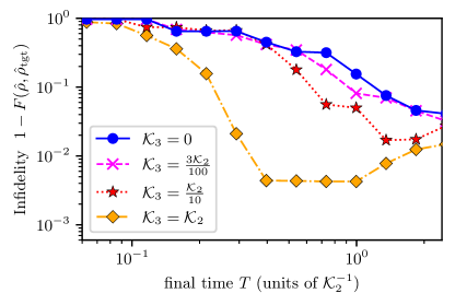
Figure 6: Results from Fig. 1, propagated with dissipation $\kappa_{\mathrm{1ph}}=\kappa_{\phi}=3\times 10^{-3}\mathcal{K}_{2}$. Due to open system dynamics, the fidelity is generalized to $F(\hat{\rho},\hat{\sigma})=\mathrm{Tr}\left\{\sqrt{\sqrt{\hat{\rho}}\hat{\sigma}\sqrt{\hat{\rho}}}\right\}^{2}$.

Fig. 6 shows the optimized results from Fig. 1 taking dissipation into account. For the dissipation strength we choose $\kappa_{1\mathrm{ph}}=\kappa_{\phi}=3\times 10^{-3}\mathcal{K}_{2}$. For all points the error, measured by the infidelity, increases substantially. However, the dash-dotted yellow curve, corresponding to the results for $\mathcal{K}_{3}=\mathcal{K}_{2}$, stands out, as it performs best of all curves. This is not surprising, as we already found that larger $\mathcal{K}_{3}$ allow for faster preparation of the cat state, as we have already observed in Fig. 1. This leads to a smaller deterioration of the optimized pulse due to dissipation and therefore smaller infidelities. Notably, the curve exhibits a plateau within $T\in[0.4\mathcal{K}_{2},1.0\mathcal{K}_{2}]$, which is due to the optimization strategy of the corresponding pulses. This strategy, which we observe for all data points on the plateau, is to keep the system in the ground state for as long as possible, while initiating the preparation only at the very end of the preparation period. As the ground state is protected against decay and the preparation time at the end of the pulse duration takes place on very similar time scales, taking dissipation into account yields comparable errors among the results of the plateau region. This demonstrates that the shorter pulse duration induced by the increase of $\mathcal{K}_{3}$ enhances the robustness of the preparation against dissipation.

References

Ofek et al. [2016]N. Ofek, A. Petrenko,
R. Heeres, P. Reinhold, Z. Leghtas, B. Vlastakis, Y. Liu, L. Frunzio, S. M. Girvin,
L. Jiang, M. Mirrahimi, M. H. Devoret, and R. J. Schoelkopf, Nature 536, 441 (2016).
Munro et al. [2002]W. J. Munro, K. Nemoto,
G. J. Milburn, and S. L. Braunstein, Physical Review A 66, 10.1103/physreva.66.023819 (2002).
van Enk and Hirota [2001]S. van
Enk and O. Hirota, Physical Review A 64, 10.1103/physreva.64.022313 (2001).
Grimm et al. [2020]A. Grimm, N. E. Frattini,
S. Puri, S. O. Mundhada, S. Touzard, M. Mirrahimi, S. M. Girvin, S. Shankar, and M. H. Devoret, Nature 584, 205 (2020).
Omran et al. [2019]A. Omran, H. Levine,
A. Keesling, G. Semeghini, T. T. Wang, S. Ebadi, H. Bernien, A. S. Zibrov, H. Pichler, S. Choi,
J. Cui, M. Rossignolo, P. Rembold, S. Montangero, T. Calarco, M. Endres, M. Greiner, V. Vuletić , and M. D. Lukin, Science 365, 570 (2019).
Glaser et al. [2015]S. J. Glaser, U. Boscain,
T. Calarco, C. P. Koch, W. Köckenberger, R. Kosloff, I. Kuprov, B. Luy, S. Schirmer, T. Schulte-Herbrüggen, D. Sugny, and F. K. Wilhelm, Eur. Phys. J. D 69, 279 (2015).
Koch et al. [2022]C. P. Koch, U. Boscain,
T. Calarco, G. Dirr, S. Filipp, S. J. Glaser, R. Kosloff, S. Montangero, T. Schulte-Herbrüggen, D. Sugny, and F. K. Wilhelm, EPJ Quantum Technol. 9, 19 (2022).
Krotov [1995]V. Krotov, Global Methods in
Optimal Control Theory (CRC Press, 1995).
Konnov and Krotov [1999]A. I. Konnov and V. F. Krotov, Autom.
Remote Control 60, 1427
(1999).
Goerz et al. [2019]M. Goerz, D. Basilewitsch,
F. Gago-Encinas,
M. G. Krauss, K. P. Horn, D. M. Reich, and C. Koch, SciPost Phys. 7, 080 (2019).
Caneva et al. [2009]T. Caneva, M. Murphy,
T. Calarco, R. Fazio, S. Montangero, V. Giovannetti, and G. E. Santoro, Phys. Rev. Lett. 103, 240501 (2009).
Leviant et al. [2022]P. Leviant, Q. Xu,
L. Jiang, and S. Rosenblum, Quantum 6, 821 (2022).
Urban et al. [2009]E. Urban, T. A. Johnson,
T. Henage, L. Isenhower, D. D. Yavuz, T. G. Walker, and M. Saffman, Nature Physics 5, 110 (2009).
Gaëtan et al. [2009]A. Gaëtan, Y. Miroshnychenko, T. Wilk, A. Chotia,
M. Viteau, D. Comparat, P. Pillet, A. Browaeys, and P. Grangier, Nature Phys 5, 115 (2009).
Balewski et al. [2014]J. B. Balewski, A. T. Krupp,
A. Gaj, S. Hofferberth, R. Löw, and T. Pfau, New J. Phys. 16, 063012 (2014).
Keating et al. [2016]T. Keating, C. H. Baldwin, Y.-Y. Jau,
J. Lee, G. W. Biedermann, and I. H. Deutsch, Physical Review Letters 117, 10.1103/physrevlett.117.213601 (2016).
Alexanian [2020]M. Alexanian, Mean number and number
variance of squeezed coherent photons in a thermal state of photons
(2020), arXiv:2004.07724 [quant-ph] .
Merkel [2009]S. Merkel, Quantum Control of D-Dimensional
Quantum Systems with Application to Alkali Atomic Spins, Ph.D. thesis, The University of New
Mexico (2009), arxiv:0906.4790 [quant-ph] .
Breuer and Petruccione [2002]H.-P. Breuer and F. Petruccione, The Theory of Open
Quantum Systems (Oxford University Press, Oxford, 2002).