IntrinsicAvatar: Physically Based Inverse Rendering of Dynamic Humans from Monocular Videos via Explicit Ray Tracing

Abstract

We present IntrinsicAvatar, a novel approach to recovering the intrinsic properties of clothed human avatars including geometry, albedo, material, and environment lighting from only monocular videos. Recent advancements in human-based neural rendering have enabled high-quality geometry and appearance reconstruction of clothed humans from just monocular videos. However, these methods bake intrinsic properties such as albedo, material, and environment lighting into a single entangled neural representation. On the other hand, only a handful of works tackle the problem of estimating geometry and disentangled appearance properties of clothed humans from monocular videos. They usually achieve limited quality and disentanglement due to approximations of secondary shading effects via learned MLPs. In this work, we propose to model secondary shading effects explicitly via Monte-Carlo ray tracing. We model the rendering process of clothed humans as a volumetric scattering process, and combine ray tracing with body articulation. Our approach can recover high-quality geometry, albedo, material, and lighting properties of clothed humans from a single monocular video, without requiring supervised pre-training using ground truth materials. Furthermore, since we explicitly model the volumetric scattering process and ray tracing, our model naturally generalizes to novel poses, enabling animation of the reconstructed avatar in novel lighting conditions.

1 Introduction

Photo-realistic reconstruction and animation of clothed human avatars is a long-standing problem in augmented reality, virtual reality, and computer vision. Existing solutions can achieve high-quality reconstruction for both geometry and appearance of clothed humans given dense multi-view cameras [20, 59, 24]. Recently, reconstruction of clothed humans from monocular videos has also been explored [54, 70, 19]. While these approaches achieve satisfactory results, they model the appearance of clothed humans as a single neural representation. This makes it difficult to edit the physical properties of the reconstructed clothed human avatars, such as reflectance and material, or to relight the reconstructed clothed human avatars under novel lighting conditions. In this work, we aim to recover physically based intrinsic properties for clothed human avatars including geometry, albedo, material, and environment lighting from only monocular videos.

Physically based inverse rendering is a challenging problem in computer graphics and computer vision. Traditional approaches tackle this problem as a pure optimization problem with simplifying assumptions such as controlled, known illumination. On the other hand, recent advances in neural fields have enabled the high-quality reconstruction of geometry and surface normals from multi-view RGB images. Given this progress, physically based inverse rendering of static scenes under unknown natural illumination has been demonstrated [29, 85]. Most recently, various works have combined human body priors with the physically based inverse rendering pipeline to reconstruct clothed human avatars with disentangled geometry, albedo, material, and lighting from monocular videos [13, 67, 25]. However, these methods either ignore physical plausibility or model secondary shading effects via approximation, resulting in limited quality of reconstructed clothed human avatars.

Two major challenges are present for physically based inverse rendering of clothed humans from monocular videos: (1) accurate geometry reconstruction, especially normal estimates are essential for high-quality inverse rendering. (2) Modeling secondary shading effects such as shadows and indirect illumination is expensive and requires a certain level of efficiency to query the underlying neural fields. Existing monocular geometry reconstruction methods of clothed humans all rely on large MLPs to achieve high-quality geometry reconstruction. However, using large MLPs negatively impacts the efficiency of secondary shading computation. Therefore, most existing methods are forced to rely on simple assumptions (no shadows, no indirect illumination) or approximations (pre-trained MLPs) to model secondary shading effects. More efficient neural field representations such as instant NGP (iNGP [47]) have proven to be effective for geometric reconstruction given multiple input views of a static scene [60, 38, 71], but it remains a challenge to extend such representation to dynamic humans under monocular setup.

In this paper, we employ iNGP with hashing-based volumetric representation and signed distance field (SDF) to achieve fast and high-quality reconstruction of clothed humans from monocular videos. The high-quality initial geometry estimation and efficiency of iNGP facilitate the modeling of inverse rendering via explicit Monte-Carlo ray tracing. Furthermore, traditional surface-based inverse rendering methods give ambiguous predictions at edges and boundaries. We propose to use volumetric scattering to model edges and boundaries in a more physically plausible way. Our experiments demonstrate that we can achieve high-quality reconstruction of clothed human avatars with disentangled geometry, albedo, material, and environment lighting from only monocular videos. In summary, we make the following contributions:

• We propose a model for fast, high-quality geometry reconstruction of clothed humans from monocular videos.

• We propose to combine volumetric scattering with the human body articulation for physically based inversed rendering of dynamic clothed humans. We use explicit Monte-Carlo ray tracing in canonical space to model the volumetric scattering process, enabling relighting for unseen poses.

• We demonstrate that our method can achieve high-quality reconstruction of clothed human avatars with disentangled geometry, albedo, material, and environment lighting from only monocular videos of clothed humans. We also show that our learned avatars can be rendered realistically under novel lighting conditions and novel poses.

We will make our code and model publicly available.

2 Related Work

Traditional Inverse Rendering: Traditional approaches to inverse rendering work on either single RGB images [4, 36, 64, 78, 61, 72, 37, 39] or multi-view, multi-modality inputs [33, 62, 51, 20, 80, 31, 49, 57, 17]. Recovering shape, reflectance, and illumination from a single RGB image is heavily underconstrained and often works poorly on real-world setups such as scene-level reconstruction and articulated object reconstruction. A more practical approach is to reconstruct shapes from multi-view RGB(D) images and make simplifying assumptions such as no shadowing and controlled lighting conditions [63, 43, 49]. This kind of approach often results in high-quality reconstruction of physical properties, but lacks flexibility and does not work under natural lighting conditions.

Physically Based Inverse Rendering with Neural Fields: Since the blossom of neural radiance fields (NeRF [46]), a variety of works have been proposed to tackle the inverse rendering problem using neural field representations. However, many works make use of simplifying assumptions such as known lighting conditions [65], ignoring shadowing effects [6, 79, 48], or assuming constant reflectance [79]. NeRFactor [81] was the first work that enabled full estimation of a scene’s underlying physical properties (geometry, albedo, BRDF, and lighting) under a single unknown natural illumination while also taking shadowing effect into account. Following the general framework of NeRFactor, InvRender [82] builds upon the state-of-the-art shape and radiance field reconstruction methods [76, 69] and proposed to model indirect illumination by distilling a pre-trained NeRF into auxiliary MLPs. NVDiffRecMC [21] tackles the inverse rendering problem by exploring the combination of mesh-based Monte-Carlo ray tracing, multiple-importance sampling, and off-the-shelf denoisers. However, it does not model indirect illumination and the surface-based inverse rendering process is known to be prone to local minima.

Most recently, TensoIR [29] takes advantage of fast radiance field data structures [8] and conducts exact visibility and indirect illumination estimation via ray marching. It also applies multi-light reconstruction to improve the reconstruction quality. In comparison to TensoIR, we use an SDF representation and combine iso-surface search technique with volumetric scattering, resulting in better visibility modeling, especially for cloth wrinkles. Most importantly, we target dynamic, animatable clothed avatar reconstruction while TensoIR focuses on static scene reconstruction.

Microfacet fields [44] proposed to utilize volumetric scattering with a surface BRDF and ad-hoc sampling strategies. Concurrent to [44] , NeMF [83] also proposed to use volumetric scattering with microflake phase functions [27, 23] to replace surface-based BRDF for volume scattering, resulting in the ability to reconstruct thin structures and low-density volumes. Both methods focus on static scenes reconstruction and relighting while using density fields to represent the underlying geometry.

Neural Radiance Fields for Human Reconstruction: Neural radiance fields have been used for human reconstruction from monocular videos. Most works [53, 52, 73, 28, 34] focus on appearance reconstruction while using density fields as a noisy geometry proxy. Some methods use SDFs to represent the geometry of humans and achieve impressive results in both geometry reconstruction and photo-realistic rendering [74, 70, 54, 19]. However, these methods bake intrinsic properties such as albedo, material, and lighting all into the learned neural representations, preventing the application of these methods in relighting and material editing.

Physically Based Inverse Rendering of Humans: High-quality 3D relightable human assets can be obtained via a multi-view, multi-modality capture system with controlled lighting [20, 5, 80] or by training regressors on high-quality digital 3D assets [3, 15, 84]. For models that directly optimize over monocular videos, RANA [25] pre-trains a mesh representation on multiple subjects with ground truth 3D digital assets while using a simplified spherical harmonics lighting model, thus cannot handle secondary shading effects such as shadows and indirect illumination. [67] propose to model the secondary shading effects via spherical Gaussian approximations, which do not handle shadowing effects. Furthermore, there is no public code or data available for this work. Relighting4D [13] jointly estimates the shape, lighting, and the albedo of dynamic humans from monocular videos under unknown illumination by approximating visibility via learned MLPs. These learned MLPs are over-smoothed approximations to real visibility values, while also having the the inherent problem of not being able to generalize to novel poses. In contrast, we employ fast, exact visibility querying via explicit ray tracing, and thus can generalize to any novel poses.

Concurrent Works:  [75] proposes a novel system for reconstructing relightable and animatable neural avatars from sparse-view (or monocular) videos. The authors design a hierarchical distance query algorithm for efficient ray-surface intersection and light visibility computation using sphere tracing. They extend DFSS to deformable neural SDF, efficiently producing realistic soft shadows for the neural avatars. However, their use of sphere tracing and surface rendering results in visible artifacts around elbows and armpits, as sphere tracing does not guarantee convergence, especially when combined with human body articulation. In contrast, we use volumetric scattering to model the human body, while also using ray marching to compute secondary ray visibilities, this results in less visual artifacts.

3 Method

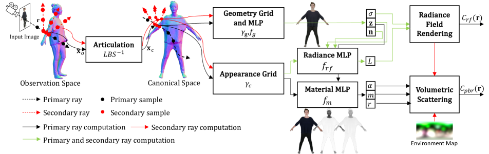
Figure 2: Inverse Rendering of Clothed Avatars with Volumetric Scattering. Given an input image and associated camera rays, we warp the rays to the canonical space and do both primary and secondary ray marching/tracing in canonical space. We model geometry with a geometry hash grid $\gamma_{g}$ and MLP $f_{g}$, while also modeling volumetric radiance and material with an appearance grid $\gamma_{c}$ and two additional MLPs $f_{rf}$, $f_{m}$. We supervise both $C_{rf}$ and $C_{pbr}$ using a L1 loss wrt.  the input image.

In this section, we first introduce basic concepts of neural radiance fields (NeRF [45]). Then we describe our framework of geometry reconstruction of clothed avatars from monocular videos. The clothed avatars are modeled as an articulated NeRF with SDF as its geometry representation. Next, we introduce the volumetric scattering process from computer graphics and draw a connection between it and NeRF. Finally, we describe our solution to secondary ray tracing of volumetric scattering, which combines the explicit ray-marching with iso-surface search and body articulation. The final outputs are intrinsic properties of clothed avatars including geometry, material, albedo, and lighting.

3.1 Background: Neural Radiance Fields

Given a ray $\mathbf{r}=(\mathbf{o},\mathbf{d})$ defined by its camera center $\mathbf{o}$ and viewing direction $\mathbf{d}$, NeRF computes the output radiance (i.e. pixel color) of the ray via:

$$C_{rf}(\mathbf{r})= \int_{t_{n}}^{t_{f}}T(t_{n},t)\sigma_{t}(\mathbf{r}(t))L(\mathbf{r}(t),-\mathbf{d})dt$$ (1)

s.t $$\mathbf{r}(t)=\mathbf{o}+t\mathbf{d}$$

$$T(t_{n},t)=\exp\left(-\int_{t_{n}}^{t}\sigma_{t}(\mathbf{r}(s))ds\right)$$

where $(t_{n},t_{f})$ defines the near/far point for the ray integral. In practice, NeRF uses a ray marching algorithm to approximate the exact value of the integral:

$$C_{rf}(\mathbf{r})\approx \sum_{i=1}^{N}w^{(i)}L(\mathbf{r}(t^{(i)}),-\mathbf{d})$$ (2)

s.t $$\mathbf{r}(t)=\mathbf{o}+t\mathbf{d}$$

$$w^{(i)}=T^{(i)}\left(1-\exp(-\sigma_{t}(\mathbf{r}(t^{(i)}))\delta^{i}\right)$$

$$T^{(i)}=\exp\left(-\sum_{j<i}\sigma_{t}(\mathbf{r}(t^{(j)}))\delta^{(j)}\right)$$

$$\delta^{(i)}=t^{(i+1)}-t^{(i)}$$

where $\{t^{(1)},\cdots,t^{(N)}\}$ are a set of sampled offsets on the ray. $\sigma_{t}(\cdot)$ and $L(\cdot,\cdot)$ are represented as either neural networks [46, 50, 69, 77], explicit grid data [66, 1], or a hybrid of both [16, 58, 47, 8, 9, 10, 14].

3.2 Clothed Humans Avatars as Articulated Neural Radiance Fields

We follow the recent approaches of modeling humans as articulated NeRF [73, 70, 34, 28]. We assume body articulations based on the SMPL model [42]. Following previous works, we define the observation space as a space where the human is observed, and the canonical space as a space where the human is in a canonical pose. We apply inverse linear blend skinning (LBS) to transform 3D points in the observation space $\mathbf{x}_{o}=\mathbf{r}(t)$ to the point in canonical space $\mathbf{x}_{c}$. We model the radiance field, materials, and albedo all in the canonical space.

Articulation via Inverse LBS: In the SMPL model, the linear blender skinning (LBS) function is defined as:

$$\mathbf{x}_{o}=\text{LBS}(\mathbf{x}_{c},\{\mathbf{B}_{b}\}_{b=1}^{B},w(\mathbf{x}_{c}))=\left(\sum_{b=1}^{B}w(\mathbf{x}_{c})_{b}\mathbf{B}_{b}\right)\mathbf{x}_{c}$$ (3)

where $\{\mathbf{B}_{b}\}_{b=1}^{B}$ are the rigid bone-transformations defined by estimated SMPL parameters. $w(\mathbf{x}_{c})$ are skinning weights of point $\mathbf{x}_{c}$. We use Fast-SNARF [12] to model the canonical skinning weight function $w(\cdot)$ and the inverse skinning function:

$$\mathbf{x}_{c}=\text{LBS}^{-1}(\mathbf{x}_{o},\{\mathbf{B}_{b}\}_{b=1}^{B},w(\mathbf{x}_{c}))$$ (4)

For simplicity, we drop the dependency on $\{\mathbf{B}_{b}\}_{b=1}^{B}$ and $w(\mathbf{x}_{c})$ for the remainder of the paper.

Geometry: We use iNGP [47] with SDF to represent the underlying canonical shape of clothed humans. Specifically, given a query point $\mathbf{x}_{c}$ in canonical space, we predict the SDF value of the point and a latent feature $\mathbf{z}$:

$$\left(\text{SDF}(\mathbf{x}_{c}),\mathbf{z}\right)=f_{g}(\gamma_{g}(\mathbf{x}_{c}))$$ (5)

where $\gamma_{g}(\cdot)$ is the iNGP hash grid feature of the input point, and $f_{g}$ is a small MLP with a width of $64$ and one hidden layer. We use VolSDF [77] to convert from SDF to density $\sigma_{t}$.

Radiance and Material: Radiance and materials are predicted as follows:

$$L(\mathbf{x}_{c},\mathbf{d}) =f_{rf}(\gamma_{c}(\mathbf{x}_{c}),\mathbf{z},\text{ref}(\mathbf{d},\mathbf{n}),\mathbf{n})$$ (6)

$$\alpha(\mathbf{x}_{c}),r(\mathbf{x}_{c}),m(\mathbf{x}_{c}) =f_{m}(\gamma_{c}(\mathbf{x}_{c}),\mathbf{z})$$ (7)

where $\gamma_{c}(\cdot)$ is the feature from another iNGP hash grid designed specifically for radiance and material prediction. The same strategy was also employed in  [60] for learning better geometric details. $f_{rf}$ and $f_{m}$ are both MLPs with a width of $64$ and two hidden layers. $\mathbf{n}$ is the analytical normal obtained from SDF fields. $\text{ref}(\mathbf{d},\mathbf{n})$ reflects the viewing direction $\mathbf{d}$ around the normal $\mathbf{n}$, similar to [68]. $L(\cdot,\cdot)$ will be used for Eq. (2) whereas $\alpha$, $r$, and $m$ are spatially varying albedo, roughness, and metallic parameters that will be used for physically based inverse rendering.

For ray marching, we use 128 uniform samples and do two rounds of importance sampling, each time with 16 samples, to obtain a final set of 160 samples per ray.

With the aforementioned model, we can quickly reconstruct the detailed geometry of clothed human avatars from a single monocular video in less than 30 minutes.

3.3 Physically Based Inverse Rendering via Volumetric Scattering

With initial geometry and radiance estimation from previous sections, we now account intrinsic properties of clothed human avatars, i.e. material, albedo, and lighting conditions for the rendering process.

With the standard equation of transfer of participating media in computer graphics [26, 55], we reach the NeRF formula Eq. (1) by assuming all the radiance that reaches the camera is modeled by neural networks. On the other hand, if we think all the radiance that reaches the camera is scattered from some light sources (e.g. environment maps) by a volume of media, while the media itself does not emit any radiance, then we are tackling the volume scattering problem.

Formally, we have the following integral to compute the radiance scattered by the volume representing the human body along a certain camera ray $(\mathbf{o},\mathbf{d})$:

$$C_{pbr}(\mathbf{r})= \int_{t_{n}}^{t_{f}}T(t_{n},t)\sigma_{s}(\mathbf{r}(t))L_{s}(\mathbf{r}(t),-\mathbf{d})dt$$ (8)

s.t $$\mathbf{r}(t)=\mathbf{o}+t\mathbf{d}$$

$$T(t_{n},t)=\exp\left(-\int_{t_{n}}^{t}\sigma_{t}(\mathbf{r}(s))ds\right)$$

$$L_{s}(\mathbf{x},-\mathbf{d})=\int_{S^{2}}f_{p}(\mathbf{x},-\mathbf{d},\bar{\mathbf{d}})L_{i}(\mathbf{x},-\bar{\mathbf{d}})d\bar{\mathbf{d}}$$

$$\sigma_{t}(\mathbf{r}(t))=\sigma_{a}(\mathbf{r}(t))+\sigma_{s}(\mathbf{r}(t))$$

$S^{2}$ is the domain of a unit sphere. $\sigma_{s}$ and $\sigma_{a}$ are the scattering coefficient and the absortion coefficient, respectively. Their sum is the attentuation coefficient, which is also known as the density in NeRF literature. $f_{p}(\mathbf{x},-\mathbf{d},\bar{\mathbf{d}})$ is the phase function that describes the probability of light scattering from direction $\bar{\mathbf{d}}$ to $-\mathbf{d}$ at point $\mathbf{x}$. $L_{i}(\mathbf{x},-\bar{\mathbf{d}})$ is the incoming radiance towards point $\mathbf{x}$ along the direction $-\bar{\mathbf{d}}$, it can be computed as a weighted sum of $C_{rf}(\mathbf{x},\bar{\mathbf{d}})$ (Eq. (1)) and radiance from an environment map $\text{Env}(\bar{\mathbf{d}})$:

$$L_{i}(\mathbf{x},-\bar{\mathbf{d}})= C_{rf}(\mathbf{x},\bar{\mathbf{d}})$$

$$+\exp\left(-\int_{t_{n^{\prime}}}^{t_{f^{\prime}}}\sigma_{t}(\mathbf{x}+s\bar{\mathbf{d}})ds\right)\text{Env}(\bar{\mathbf{d}})$$ (9)

where $t_{n^{\prime}}$ and $t_{f^{\prime}}$ are the near and far points of secondary rays. In traditional physically based rendering, the first term represents indirect illumination while the second term represents direct illumination. Instead of modeling indirect illumination with path tracing, we use the trained radiance field to approximate it. This is also done in various recent works [29, 82] for modeling static scenes from multi-view input images. For Monte-Carlo estimation of $C_{pbr}(\mathbf{r})$, we will have to sample the two integrals $\int_{t_{n}}^{t_{f}}$ and $\int_{S^{2}}$ separately. The first integral is estimated via quadrature as was done in standard NeRF rendering. We next describe how to sample the second integrals.

For approximating Eq. (8), we importance sample offsets $\{\bar{t}^{(1)},\cdots,\bar{t}^{(M)}\}$ from the PDF estimated by radiance field samples that have been used to estimate Eq. (2) (see Fig. 3). The approximated Eq. (8) becomes:

$$C_{pbr}(\mathbf{r})\approx \sum_{i=1}^{M}w^{(i)}\frac{\sigma_{s}(\mathbf{r}(\bar{t}^{(i)}))}{\sigma_{t}(\mathbf{r}(\bar{t}^{(i)}))}L_{s}(\mathbf{r}(\bar{t}^{(i)}),-\mathbf{d})$$ (10)

s.t $$\mathbf{r}(t)=\mathbf{o}+t\mathbf{d}$$

$$w^{(i)}=T^{(i)}\left(1-\exp(-\sigma_{t}(\mathbf{r}(\bar{t}^{(i)})\delta^{(i)})\right)$$

$$T^{(i)}=\exp\left(-\sum_{j<i}\sigma_{t}(\mathbf{r}(\bar{t}^{(j)}))\delta^{(j)}\right)$$

$$L_{s}(\mathbf{r}(\bar{t}^{(i)}),-\mathbf{d})=\frac{f_{p}(\mathbf{r}(\bar{t}^{(i)}),-\mathbf{d},\bar{\mathbf{d}}^{(i)})}{\text{pdf}(\bar{\mathbf{d}}^{(i)})}$$

$$\qquad\qquad\qquad\qquad\cdot L_{i}(\mathbf{r}(\bar{t}^{(i)}),-\bar{\mathbf{d}}^{(i)})$$

$$\sigma_{t}(\mathbf{r}(t))=\sigma_{a}(\mathbf{r}(t))+\sigma_{s}(\mathbf{r}(t))$$

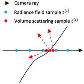
Figure 3: Sampling for Volumetric Scattering

in which $\frac{\sigma_{s}(\mathbf{r}(\bar{t}^{(i)}))}{\sigma_{t}(\mathbf{r}(\bar{t}^{(i)}))}$ corresponds to the spatially varying albedo and is analogous to that in surface-based rendering. $\text{pdf}(\bar{\mathbf{d}}^{(i)})$ is the PDF from which $\bar{\mathbf{d}}^{(i)}$ is sampled.

Essentially, we use quadrature to estimate the first integral $\int_{t_{n}}^{t_{f}}$, and Monte-Carlo sampling to estimate the second integral $\int_{S^{2}}$, all together with $M$ samples. We refer readers to Appendix A for a detailed derivation of Eq. (10). During training $\bar{\mathbf{d}}^{(i)}$ is uniformly sampled from the unit sphere with $M=512$ and stratified jittering [56]. For relighting, we use light importance sampling with $M=1024$ to sample from a known environment map.

We note that when using an SDF-density representation, most of the samples $\bar{t}^{(i)}$ are concentrated around the surface of the human body. This makes the volumetric scattering process similar to a surface-based rendering process. For the rays where a zero-crossing of SDF values can be found, we use the point before the first negative SDF value as the starting point of secondary ray tracing to avoid starting from inside surfaces. On the other hand, rays at edges and boundaries may not have a well-defined surface, for these rays, it would be difficult to employ surface-based rendering while volume scattering suits naturally for this case.

We use a simplified version of Disney BRDF [7] to model the combined effect of the volumetric albedo $\frac{\sigma_{s}(\mathbf{r}(\bar{t}^{(i)}))}{\sigma_{t}(\mathbf{r}(\bar{t}^{(i)}))}$ and the phase function $f_{p}$. It takes predicted albedo $\alpha$, roughness $r$ and metallic $m$ as inputs:

$$\frac{\sigma_{s}}{\sigma_{t}}f_{p}(\mathbf{\omega}_{o},\mathbf{\omega}_{i})=\text{BRDF}(\mathbf{\omega}_{o},\mathbf{\omega}_{i},\alpha,r,m,\mathbf{n})\max\left(\mathbf{n}\cdot\mathbf{\omega}_{i},0\right)$$

We drop dependency on spatial locations for brevity. An extended implementation detail of the above BRDF can be found in Appendix B. More physically accurate phase functions for rendering surface-like volumes, such as SGGX [23] can also be plugged into our formulation, but we empirically do not find them providing any advantage for our application.

3.4 Articulated Secondary Ray Tracing

Given the $M$ samples $\{\bar{t}^{(i)}\}_{i=1}^{M}$ on a primary ray, we trace secondary rays for each of the samples, such that we could compute opacity (or visibility in a surface rendering setup) and radiance for each of the secondary ray. Formally, we trace a secondary ray $\bar{\mathbf{r}}^{(i)}$ from the corresponding sample, where $\bar{\mathbf{r}}^{(i)}=(\bar{\mathbf{o}}^{(i)},\bar{\mathbf{d}}^{(i)})$ with $\bar{\mathbf{o}}^{(i)}=\mathbf{r}(\bar{t}^{(i)})$.

Secondary Ray Tracing: We note that traditional sphere tracing could lead to non-convergence rays when the SDF is not smooth. This is exacerbated when the SDF is approximated by neural networks and combined with body articulation. Furthermore, the sequential evaluation of SDF values on a ray is not amenable to parallelization, especially when a large number of secondary rays need to be evaluated and each evaluation involves neural networks.

Given the underlying NeRF representation, precise surface location is often not required to compute radiance, while the opacity is binary most of the time due to the SDF-density representation. This motivates us to use ray marching to compute secondary shading effects. However, we observe that the Laplace density function of [77] tends to assign non-negligible density values to small positive SDF values. This will cause the secondary ray marching to give non-zero weights to points that are very close to the surface, i.e. starting points $\bar{\mathbf{o}}$’s of secondary rays. While NeuS [69] is more well-behaved as it only assigns high weights for SDF zero-crossing intervals, estimating weights of ray segments requires estimation of analytical surface normals, which usually doubles the computation cost of ray marching.

Motivated by these facts, we propose a hybrid approach to secondary ray marching by searching for the first SDF zero-crossing point of a set of uniform samples on the secondary ray and only start accumulating importance weights from that point. Given the weights of uniform samples, we sample 4 additional samples on the secondary ray and compute the transmittance and radiance from these 4 samples. The computed transmittance and radiance are inputs to incoming radiance evaluation Eq. (3.3).

Formally, given a secondary ray $\bar{\mathbf{r}}$, we first uniformly sample 64 offsets $\{t^{\prime(1)},\cdots,t^{\prime(64)}\}$ on the ray between the near and far points, $t_{n^{\prime}}=0$ $t_{f^{\prime}}=1.5$. Each of the sampled offsets is transformed to the canonical space to query its SDF value:

$$\text{SDF}(\bar{\mathbf{r}}(t^{\prime}))=f_{g}(\gamma_{g}(\text{LBS}^{-1}(\bar{\mathbf{r}}(t^{\prime}))))$$ (11)

Alg. 1 describes the procedure of searching for the first zero-crossing point and accumulating weights for each of the points.

Algorithm 1 Zero-Crossing Search and Importance Weight Accumulation

0:  $\{\text{SDF}(\bar{\mathbf{r}}(t^{\prime(i)}))\}_{i=1}^{64}$, $\bar{\mathbf{r}}=(\bar{\mathbf{o}},\bar{\mathbf{d}})$

0:  Importance weights $\{w^{(i)}\}_{i=1}^{63}$

1:  $s\leftarrow 1$

2:  $\{w^{(i)}\}_{i=1}^{63}\leftarrow\mathbf{0}$

3:  while $s<63$ do

4:     if $\text{SDF}(\bar{\mathbf{r}}(t^{\prime(s)}))\cdot\text{SDF}(\bar{\mathbf{r}}(t^{\prime(s+1)}))<0$ then

5:        break

6:     end if

7:     $s\leftarrow s+1$

8:  end while

9:  $T(\bar{\mathbf{r}})\leftarrow 1$

10:  for $i=s$ to $63$ do

11:     $\delta^{(i)}\leftarrow t^{\prime(i+1)}-t^{\prime(i)}$

12:     $w^{(i)}\leftarrow\left(1-\exp(-\sigma_{t}(\bar{\mathbf{r}}(t^{\prime(i)}))\delta^{(i)})\right)T(\bar{\mathbf{r}})$

13:     $T(\bar{\mathbf{r}})\leftarrow T(\bar{\mathbf{r}})\exp\left(-\sigma_{t}(\bar{\mathbf{r}}(t^{\prime(i)}))\delta^{(i)}\right)$

14:  end for

15:  return  $\{w^{(i)}\}_{i=1}^{63}$

This is similar to the traditional sphere tracing algorithm, with the difference that SDF values are evaluated uniformly in parallel instead of sequentially. We also parallelize the search of zero-crossing points and weight accumulation over rays with custom CUDA implementation.

Temporal Occupancy Grids: Another technique to reduce computation is to maintain an occupancy grid to mark occupied voxels during training and skip unoccupied voxels during ray marching/tracing [47, 1, 8, 35] . This also applies to temporal reconstruction as one can define the occupancy grid as the union of all shapes from different time steps [28]. To further reduce the computational cost, we employ a 4D occupancy grid structure in which we maintain a $64^{3}$ occupancy grid for each training frame. At the beginning of training, we first use a single occupancy grid for all frames. After we have attained a reasonable SDF we re-initialize the occupancy grid for each frame using the learned canonical SDF.

3.5 Training Details

We use standard L1 loss wrt. input images on radiance predicted by both radiance field (RF loss) and volumetric scattering (PBR loss). We apply eikonal loss [18] (throughout training) and curvature loss [60] (only the first half of the training) to regularize the SDF field. We also apply Lipschitz regularization [60] and standard smoothness regularization [81, 29] to the material predictions. Details on losses and hyperparameters can be found in Appendix C.1.

We train a total of 25k iterations with a learning rate of $0.001$ decayed by a factor of $0.3$ at $12.5$k, $18.75$k, $22.5k$, and $23.75$k iterations, respectively. The first 10k iterations are trained with the RF loss only, while the rest of the iterations are trained on both the RF loss and the PBR loss. We use a batch size of $4096$ rays. Training is done on a single NVIDIA RTX 3090 GPU in 4 hours.

4 Experimental Evaluation

4.1 Datasets

We utilize 3 different datasets to conduct our experiments

• RANA [25] To quantitatively evaluate our estimation of the physical properties of the reconstructed avatar, we use 8 subjects from the RANA dataset. The dataset is rendered using a standard path tracing algorithm, with ground truth albedo, normal, and relighted images available for evaluation. We follow protocol A in which the training set resembles a person holding an A-pose rotating in front of the camera under unknown illumination. The test set consists of images of the same subject in random poses under novel illumination conditions.

• PeopleSnapshot [2] In PeopleSnapshot, subjects always hold a simple A-pose and rotate in front of the camera under natural illumination. We use 4 subjects from the dataset with refined pose estimation from [11, 28].

• SyntheticHuman-Relit To additionally evaluate relighting on training poses of continuous videos, we create a synthetic dataset by rendering two subjects from the SyntheticHuman dataset [54] with Blender under different illumination conditions. Due to space limits, we refer readers to the Appendix D and E for details and results on this dataset.

4.2 Baselines

To our knowledge, Relighting 4D (R4D [13]) is the only baseline with publicly available code for the physically based inversed rendering of clothed human avatars under unknown illumination, without pretraining on any ground truth geometry/albedo/materials. RANA [25] only provides public access to their data but not the code. Furthermore, RANA pretrains on ground truth albedo, which is not available in our setting.

We note that the original R4D implementation does not employ any mask loss. We therefore also report a variant of R4D (denoted as R4D*) that employs a mask loss. R4D* achieves overall better performance than R4D (Tab. 1) and thus we primarily compared our method to this improved version of R4D.

4.3 Evaluation Metrics

On synthetic datasets, we evaluate the following metrics:

• Albedo PNSR/SSIM/LPIPS we evaluate the standard image quality metrics on albedos rendered under training views. Due to ambiguity in estimating albedo and light intensity, we follow the practice of [81] to align the predicted albedo with the ground truth albedo. More details can be found in Appendix C.2.

• Normal Error this metric evaluates normal estimation error (in degrees) between predicted normal images and the ground-truth normal images.

• Relighting PSNR/SSIM/LPIPS we also evaluate image quality metrics on images synthesized on novel poses with novel illumination. Relighting evaluation on training poses (i.e. SyntheticHuman-Relit dataset) is reported in Appendix E.

On real-world datasets, i.e. PeopleSnapshot, we primarily present qualitative results including novel view/pose synthesis under novel illuminations.

4.4 Comparison to Baselines

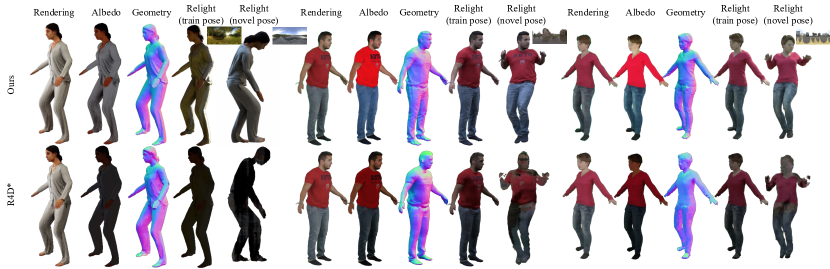
Figure 4: Qualitative comparison to the baseline. We show the results of our method and R4D* on both synthetic (left) and real (middle, right) datasets. As indicated, R4D* struggles to recover intrinsic properties of avatars and do not produce realistic relighting results. Furthermore, it fails to generalize to novel poses. Our method produces high-quality results on both synthetic and real datasets, while generalizing well to novel poses and illuminations. More qualitative results can be found in Appendix F

Method	Albedo			Normal	Relighting (Novel Pose)
	PSNR $\uparrow$	SSIM $\uparrow$	LPIPS $\downarrow$	Error $\downarrow$	PSNR $\uparrow$	SSIM $\uparrow$	LPIPS $\downarrow$
R4D	18.24	0.7780	0.2414	42.69 °	14.37	0.8133	0.2017
R4D*	18.23	0.8254	0.2043	27.38 °	16.62	0.8370	0.1726
Ours	22.83	0.8816	0.1617	9.96 °	18.18	0.8722	0.1279

Table 1: Quantitative comparison to the baseline on the RANA dataset.

We present the average metrics on the RANA dataset in Tab. 1. Our method significantly outperforms R4D and R4D* on all metrics, achieving 77% and 64% reduction in the normal estimation error, respectively. This combined with our explicit ray tracing technique also gives us a significant improvement in albedo-related metrics on training poses.

For relighting novel poses, we note that the SMPL model is not perfectly aligned with images in the RANA dataset, which could make the PSNR metric less meaningful. Thus we argue that SSIM and LPIPS can better reflect the quality of the relighting results. Nevertheless, R4D* fails to produce reasonable results due to its inability to generalize to novel poses. On the other hand, our method can produce high-quality re-posing and relighting results (Fig. 4).

4.5 Ablation Study

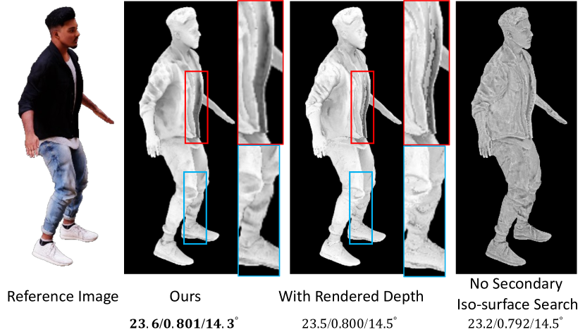
Figure 5: Ablation study. We visualize average visibility (AV) maps of each variant and report albedo PSNR ($\uparrow$)/albedo SSIM ($\uparrow$)/Normal Error ($\downarrow$). Surface scattering with rendered depth results in discontinuities at boundaries and edges. Without our proposed iso-surface search for secondary ray tracing, the visibility map is much darker and does not reflect true visibility.

In this section, we ablate several of our design choices. We use subject 01 from the RANA dataset for this ablation study. We bootstrap the geometry with the radiance field loss for 10k iterations and then optimize only wrt. to the PBR loss. This way we can isolate the effect of different design choices for PBR. We visualize average visibility (AV) maps which best reflect the quality of the reconstruction geometry and secondary ray tracing. The AV value of a primary ray $\mathbf{r}$ is defined as:

$$\text{AV}(\mathbf{r})=2*\frac{1}{M}\sum_{i=1}^{M}V(\bar{\mathbf{r}}^{(i)})$$ (12)

where $V(\bar{\mathbf{r}}_{i})$ is the visibility of the $i$-th secondary ray (1 for not occluded, 0 for occluded), and $M$ is the number of secondary rays sampled for each primary ray. We multiply visibility by 2 as we sample secondary rays on a unit sphere instead of a hemisphere. The results are summarized in Fig. 5. We describe different variants in the following:

• Ours: Our full method with all the components described in Section 3.

• Rendered Depth with Surface Scattering: This variant corresponds to [29] that uses rendered depth and surface scattering.

• No Iso-surface Search for Secondary Ray Tracing: In this variant we do not perform the iso-surface search for secondary ray tracing (Sec. 3.4) and start accumulating weights from the first sample of the 64 samples on the secondary ray.

5 Conclusion

We have presented a novel approach to the inverse rendering of dynamic humans from only monocular videos. Our method can achieve high-quality reconstruction of clothed human avatars with disentangled geometry, albedo, material, and environment lighting from only monocular videos. We have also shown that our learned avatars can be rendered realistically under novel lighting conditions and novel poses. Experiment results show that our method significantly outperforms the state-of-the-art method both qualitatively and quantitatively. We discuss limitations and future work in Appendix G.

6 Acknowledgment

We thank Umar Iqbal and Zhen Xu for the helpful discussion on setting up synthetic datasets. We thank Zijian Dong and Naama Pearl for constructive feedback on our early draft. SW, BA and AG were supported by the ERC Starting Grant LEGO-3D (850533) and the DFG EXC number 2064/1 - project number 390727645. SW and ST acknowledge the SNF grant 200021 204840.

Appendix A Volume Scattering Derivation

In this section, we derive the volume scattering approximation equation (Eq. (10) in the main paper) from the equation of transfer [55]. The general equation of transfer accounting for both volume emission and volume scattering is as follows:

$$C_{pbr}(\mathbf{r}) =\int_{t_{n}}^{t_{f}}T(t_{n},t)\sigma_{t}(\mathbf{r}(t))L(\mathbf{r}(t),-\mathbf{d})dt$$ (A.1)

s.t $$\mathbf{r}(t)=\mathbf{o}+t\mathbf{d}$$

$$T(t_{n},t)=\exp\left(-\int_{t_{n}}^{t}\sigma_{t}(\mathbf{r}(s))ds\right)$$

$$\sigma_{t}(\mathbf{r}(t))=\sigma_{a}(\mathbf{r}(t))+\sigma_{s}(\mathbf{r}(t))$$

As defined in the main paper, $\sigma_{s}$ and $\sigma_{a}$ are the scattering coefficient and the absorption coefficient, respectively. They define the probability of light being scattered/absorbed by the participating media per unit length. $\sigma_{t}$ is the attenuation coefficient, which is the sum of $\sigma_{s}$ and $\sigma_{a}$. Physically, it describes the probability of light being either out-scattered or absorbed per unit length, both of which will reduce the amount of radiance that reaches the camera. With some abuse of notation, we define $L$ as the radiance accounting for both volume emission and volume scattering:

$$L(\mathbf{r}(t),-\mathbf{d}) =\frac{\sigma_{a}(\mathbf{r}(t))}{\sigma_{t}(\mathbf{r}(t))}L_{e}(\mathbf{r}(t),-\mathbf{d})+\frac{\sigma_{s}(\mathbf{r}(t))}{\sigma_{t}(\mathbf{r}(t))}L_{s}(\mathbf{r}(t),-\mathbf{d})$$ (A.2)

s.t. $$L_{s}(\mathbf{x},-\mathbf{d})=\int_{S^{2}}f_{p}(\mathbf{x},-\mathbf{d},\bar{\mathbf{d}})L_{i}(\mathbf{x},-\bar{\mathbf{d}})d\bar{\mathbf{d}}$$

where $L_{e}$ is the volume emission radiance, $L_{s}$ is the volume scattering radiance. Since we assume the scene (human body) does not emit energy itself, $L_{e}$ should always be 0. $L_{i}$ is the incoming radiance via either direct illumination or indirect illumination, as described in Eq. (3.3) in the main paper. $f_{p}(\mathbf{x},-\mathbf{d},\bar{\mathbf{d}})$ is the phase function that describes the probability of light scattering from direction $\bar{\mathbf{d}}$ to $-\mathbf{d}$ at point $\mathbf{x}$. Given these facts, Eq. (A.1) can be re-written as:

$$C_{pbr}(\mathbf{r})= \int_{t_{n}}^{t_{f}}T(t_{n},t)\sigma_{s}(\mathbf{r}(t))L_{s}(\mathbf{r}(t),-\mathbf{d})dt$$ (A.3)

s.t $$\mathbf{r}(t)=\mathbf{o}+t\mathbf{d}$$

$$T(t_{n},t)=\exp\left(-\int_{t_{n}}^{t}\sigma_{t}(\mathbf{r}(s))ds\right)$$

$$L_{s}(\mathbf{x},-\mathbf{d})=\int_{S^{2}}f_{p}(\mathbf{x},-\mathbf{d},\bar{\mathbf{d}})L_{i}(\mathbf{x},-\bar{\mathbf{d}})d\bar{\mathbf{d}}$$

$$\sigma_{t}(\mathbf{r}(t))=\sigma_{a}(\mathbf{r}(t))+\sigma_{s}(\mathbf{r}(t))$$

which corresponds to Eq. (8) in the main paper. We next describe how to further approximate Eq. (A.3) with discrete samples.

The general idea is to sample offsets from the probability density function (PDF) of $T(t_{n},t)$ and approximate the integral with Monte-Carlo integration. Define $\text{pdf}(t)$ as the PDF of $t$ from which we sample $M$ offsets $\{\bar{\mathbf{t}}^{(i)}\}_{i=1}^{M}$, we have:

$$C_{pbr}(\mathbf{r})\approx \frac{1}{M}\sum_{i=1}^{M}\frac{T(t_{n},\bar{t}^{(i)})\sigma_{s}(\mathbf{r}(\bar{t}^{(i)}))}{\text{pdf}(\bar{t}^{(i)})}L_{s}(\mathbf{r}(\bar{t}^{(i)}),-\mathbf{d})$$ (A.4)

in the next two subsections, we describe how to sample from $\text{pdf}(t)$.

A.1 Homogeneous Volume

If we assume homogeneous volume, i.e. $\sigma_{t}(\mathbf{r}(t))=\sigma_{t}$, then we can simplify $T(t_{n},t)$ according to Beer’s law:

$$T(t_{n},t)=\exp\left(-\sigma_{t}|t-t_{n}|\right)$$ (A.5)

Sampling from $T(t_{n},t)$ is equivalent to sampling from an exponential distribution, where the PDF is given by:

$$\text{pdf}(t)=c\exp\left(-\sigma_{t}|t-t_{n}|\right)$$ (A.6)

where $c$ is a normalization constant. The cumulative distribution function (CDF) of $t$ should satisfy:

$$\int_{t_{n}}^{\infty}c\exp\left(-\sigma_{t}|t-t_{n}|\right)dt=-\frac{c}{\sigma_{t}}\exp\left(-\sigma_{t}|t-t_{n}|\right)\Big{|}_{t_{n}}^{\infty}=\frac{c}{\sigma_{t}}=1$$ (A.7)

thus $c=\sigma_{t}$ and we have the following PDF and CDF of $t$ accordingly:

$$\text{pdf}(t)= \sigma_{t}\exp\left(-\sigma_{t}|t-t_{n}|\right)$$ (A.8)

$$P(t)= 1-\exp\left(-\sigma_{t}|t-t_{n}|\right)$$ (A.9)

A.2 Heterogeneous Volume

If the homogeneous assumption is lifted, we can still approximate the integral by dividing the ray segment $(t_{n},t_{f})$ into intervals and assuming $\sigma_{t}$ to be constant within each interval. This gives us the ray marching algorithm.

Formally, let us assume the ray segment is divided into $M$ intervals, each defined by $[\bar{t}^{(1)},\bar{t}^{(2)}),\cdots[\bar{t}^{(i)},\bar{t}^{(i+1)}),\cdots[\bar{t}^{(M)},\bar{t}^{(M+1)})$ with $\bar{t}^{(1)}=t_{n},\bar{t}^{(M+1)}=t_{f}$. With our assumption on constant $\sigma_{t}$ inside each interval, i.e. $\sigma_{t}(\mathbf{r}(t))=\sigma_{t}(\mathbf{r}(\bar{t}^{(i)})),\forall t\in[\bar{t}^{(i)},\bar{t}^{(i+1)})$, define $\delta^{(i)}=|\bar{t}^{(i+1)}-\bar{t}^{(i)}|$, we define the following:

$$T(\bar{t}^{(i)},\bar{t}^{(i+1)})= \exp\left(-\sigma(\mathbf{r}(\bar{t}^{(i)}))\delta^{(i)}\right),\forall i\in\{1,\cdots,M\}$$

$$T(\bar{t}^{(1)},\bar{t}^{(i)})= \prod_{j<i}T(\bar{t}^{(j)},\bar{t}^{(j+1)})$$

$$T(\bar{t}^{(1)},\bar{t}^{(1)})= 1$$

To obtain the exact PDF from which we sample $t$, we extend Eq. (A.5) such that we sample from $T(\bar{t}^{(1)},t)$ that contains a homogeneous part and a heterogeneous part:

$$T(\bar{t}^{(1)},t)= T(\bar{t}^{(i)},t)T(\bar{t}^{(1)},\bar{t}^{(i)})$$ (A.10)

s.t. $$\bar{t}^{(i)}\leq t<\bar{t}^{(i+1)}$$

where $T(\bar{t}^{(1)},\bar{t}^{(i)})$ is the accumulated transmittance from the heterrogeneous volume before $\bar{t}^{(i)}$. Similar to Eq. (A.6) and Eq. (A.7) we can derive the normalization constant as $\sigma_{t}(\mathbf{r}(\bar{t}^{(i)}))T(\bar{t}^{(1)},\bar{t}^{(i)})$, thus the PDF of $t$ is:

$$\text{pdf}(t)= \sigma_{t}(\mathbf{r}(\bar{t}^{(i)}))T(\bar{t}^{(i)},t)T(\bar{t}^{(1)},\bar{t}^{(i)})$$

$$= \sigma_{t}(\mathbf{r}(\bar{t}^{(i)}))T(\bar{t}^{(1)},t)$$ (A.11)

s.t. $$\bar{t}^{(i)}\leq t<\bar{t}^{(i+1)}$$

Given this definition of pdf(t), we have the following CDF of $t\in[t_{n},t_{f}]$:

$$P(t)= \sum_{i=1}^{M^{\prime}}\int_{\bar{t}^{(i)}}^{\bar{t}^{(i+1)}}\text{pdf}(s)\cdot ds$$

$$= \sum_{i=1}^{M^{\prime}}\int_{\bar{t}^{(i)}}^{\bar{t}^{(i+1)}}\sigma_{t}(\mathbf{r}(\bar{t}^{(i)}))\exp\left(-\int_{\bar{t}^{(1)}}^{s}\sigma_{t}(\mathbf{r}(t^{\prime}))dt^{\prime}\right)\cdot ds$$

$$= \sum_{i=1}^{M^{\prime}}\int_{\bar{t}^{(i)}}^{\bar{t}^{(i+1)}}\sigma_{t}(\mathbf{r}(\bar{t}^{(i)}))\exp\left(-\int_{\bar{t}^{(1)}}^{\bar{t}^{(i)}}\sigma_{t}(\mathbf{r}(t^{\prime}))dt^{\prime}-\int_{\bar{t}^{(i)}}^{s}\sigma_{t}(\mathbf{r}(t^{\prime}))dt^{\prime}\right)\cdot ds$$

$$= \sum_{i=1}^{M^{\prime}}\int_{\bar{t}^{(i)}}^{\bar{t}^{(i+1)}}\sigma_{t}(\mathbf{r}(\bar{t}^{(i)}))\exp\left(-\int_{\bar{t}^{(1)}}^{\bar{t}^{(i)}}\sigma_{t}(\mathbf{r}(t^{\prime}))dt^{\prime}\right)\exp\left(-\int_{\bar{t}^{(i)}}^{s}\sigma_{t}(\mathbf{r}(t^{\prime}))dt^{\prime}\right)\cdot ds$$

$$= \sum_{i=1}^{M^{\prime}}\int_{\bar{t}^{(i)}}^{\bar{t}^{(i+1)}}\sigma_{t}(\mathbf{r}(\bar{t}^{(i)}))T(\bar{t}^{(1)},\bar{t}^{(i)})T(\bar{t}^{(i)},s)\cdot ds$$

$$= \sum_{i=1}^{M^{\prime}}T(\bar{t}^{(1)},\bar{t}^{(i)})\int_{\bar{t}^{(i)}}^{\bar{t}^{(i+1)}}\sigma_{t}(\mathbf{r}(\bar{t}^{(i)}))T(\bar{t}^{(i)},s)\cdot ds$$ (A.12)

where $M^{\prime}$ satisfies $\bar{t}^{(M^{\prime})}\leq t<\bar{t}^{(M^{\prime}+1)}$.

plug Eq. (A.9) into Eq. (A.12), we have the CDF of $t$ as:

$$P(t)= \sum_{i=1}^{M^{\prime}}T(\bar{t}^{(1)},\bar{t}^{(i)})\left(1-\exp\left(-\sigma_{t}(\mathbf{r}(\bar{t}^{(i)}))\delta^{(i)}\right)\right),\quad\bar{t}^{(M^{\prime})}\leq t<\bar{t}^{(M^{\prime}+1)}$$ (A.13)

which is a piece-wise constant CDF, and we can sample points from such CDF by standard invert CDF method as was employed in the Vanilla NeRF [46].

Plug Eq. (A.2) into Eq. (A.4), one will note that the $T(t_{n},t)$ term is in both the numerator and the denominator. Thus Eq. (A.4) simplifies to:

$$C_{pbr}(\mathbf{r})\approx \frac{1}{M}\sum_{i=1}^{M}\frac{\sigma_{s}(\mathbf{r}(\bar{t}^{(i)}))}{\sigma_{t}(\mathbf{r}(\bar{t}^{(i)}))}L_{s}(\mathbf{r}(\bar{t}^{(i)}),-\mathbf{d})$$ (A.14)

Since we define the combined effect of $\frac{\sigma_{s}(\mathbf{r}(\bar{t}^{(i)}))}{\sigma_{t}(\mathbf{r}(\bar{t}^{(i)}))}$ and the phase function as a BRDF function, which becomes unrelated to $\sigma_{t}$, while we also need to be able to differentiate wrt. the geometry represented by $\sigma_{t}$, we use quadrature weights $\{w^{(i)}\}$ from NeRF [46], resulting in Eq. (10) in the main paper:

$$C_{pbr}(\mathbf{r})\approx \sum_{i=1}^{M}w^{(i)}\frac{\sigma_{s}(\mathbf{r}(\bar{t}^{(i)}))}{\sigma_{t}(\mathbf{r}(\bar{t}^{(i)}))}L_{s}(\mathbf{r}(\bar{t}^{(i)}),-\mathbf{d})$$ (A.15)

s.t $$\mathbf{r}(t)=\mathbf{o}+t\mathbf{d}$$

$$w^{(i)}=T^{(i)}\left(1-\exp(-\sigma_{t}(\mathbf{r}(\bar{t}^{(i)})\delta^{(i)})\right)$$

$$T^{(i)}=\exp\left(-\sum_{j<i}\sigma_{t}(\mathbf{r}(\bar{t}^{(j)}))\delta^{(j)}\right)$$

$$L_{s}(\mathbf{r}(\bar{t}^{(i)}),-\mathbf{d})=\frac{f_{p}(\mathbf{r}(\bar{t}^{(i)},-\mathbf{d},\bar{\mathbf{d}}^{(i)})}{\text{pdf}(\bar{\mathbf{d}}^{(i)})}L_{i}(\mathbf{r}(\bar{t}^{(i)},-\bar{\mathbf{d}}^{(i)})$$

$$\sigma_{t}(\mathbf{r}(t))=\sigma_{a}(\mathbf{r}(t))+\sigma_{s}(\mathbf{r}(t))$$

Appendix B BRDF Definition

As mentioned in the main paper, we use a simplified version of Disney BRDF [7] to model the combined effect of the volumetric albedo $\frac{\sigma_{s}(\mathbf{r}(\bar{t}^{(i)}))}{\sigma_{t}(\mathbf{r}(\bar{t}^{(i)}))}$ and the phase function $f_{p}$. It takes predicted albedo $\alpha$, roughness $r$ and metallic $m$ as inputs:

$$\frac{\sigma_{s}}{\sigma_{t}}f_{p}(\mathbf{\omega}_{o},\mathbf{\omega}_{i}) =\text{BRDF}(\mathbf{\omega}_{o},\mathbf{\omega}_{i},\alpha,r,m,\mathbf{n})\max\left(\mathbf{n}\cdot\mathbf{\omega}_{i},0\right)$$ (B.1)

where $\mathbf{\omega}_{o}$ and $\mathbf{\omega}_{i}$ are the outgoing and incoming directions (i.e. surface to camera direction and surface to light direction, respectively). $\mathbf{\omega}_{h}$ is the half vector between $\mathbf{\omega}_{o}$ and $\mathbf{\omega}_{i}$, i.e. $\mathbf{\omega}_{h}=\frac{\mathbf{\omega}_{o}+\mathbf{\omega}_{i}}{\|\mathbf{\omega}_{o}+\mathbf{\omega}_{i}\|}$. $\mathbf{n}$ is the surface normal. The BRDF is defined as follows:

$$\text{BRDF}(\mathbf{\omega}_{o},\mathbf{\omega}_{i},\alpha,r,m,\mathbf{n})=(1-m)\frac{\alpha}{\pi}+\frac{F(\mathbf{\omega}_{o},\alpha,m)D(\mathbf{\omega}_{h},\mathbf{n},r)G(\mathbf{\omega}_{o},\mathbf{\omega}_{i},\mathbf{n})}{4(\mathbf{n}\cdot\mathbf{\omega}_{o})(\mathbf{n}\cdot\mathbf{\omega}_{i})}$$ (B.2)

in which the term $(1-m)\frac{\alpha}{\pi}$ is the diffuse component while the remaining are specular components. For the specular component, $F$ is the Fresnel-Schlick approximation to the exact Fresnel term, $D$ is the isotropic GGX microfacet distribution [22] and $G$ is Smith’s shadowing term. They are defined as follows:

$$F(\mathbf{\omega}_{o},\alpha,m) =F_{0}(\alpha,m)+(1-F_{0}(\alpha,m))2^{(-5.55473\mathbf{\omega}_{o}\cdot\mathbf{\omega}_{h}-6.98316)\mathbf{\omega}_{o}\cdot\mathbf{\omega}_{h}}$$ (B.3)

$$D(\mathbf{\omega}_{h},\mathbf{n},r) =\frac{r^{2}}{\pi((\mathbf{n}\cdot\mathbf{\omega}_{h})^{2}(r^{2}-1)+1)^{2}}$$ (B.4)

$$G(\mathbf{\omega}_{o},\mathbf{\omega}_{i},\mathbf{n}) =G_{1}(\mathbf{\omega}_{o},\mathbf{n})G_{1}(\mathbf{\omega}_{i},\mathbf{n})$$ (B.5)

s.t. $$F_{0}(\alpha,m)=0.04(1-m)+\alpha m$$

$$G_{1}(\mathbf{\omega},\mathbf{n})=\frac{(\mathbf{n}\cdot\mathbf{\omega})}{(\mathbf{n}\cdot\mathbf{\omega})(1-k)+k}\quad\text{and}\quad k=\frac{(r+1)^{2}}{8}$$

note that for $F$, instead of the typical Schlick approximation, we use the approximation from [30] which is slightly more efficient. $G_{1}$ is the Schlick-GGX approximation to the exact Smith’s shadowing term.

Appendix C Implementation Details

In this section, we provide more details about the implementation of our method.

C.1 Loss Function

In this subsection, we define $I^{(p)}\in[0,1]^{3}$ as the $p$-th pixel’s color of the input image, $C_{rf}(\mathbf{r}^{(p)})\in[0,1]^{3}$ as the predicted pixel color of the radiance field, $C_{pbr}(\mathbf{r}^{(p)})\in[0,1]^{3}$ as the predicted pixel color of the physically based rendering, $\mathbf{M}^{(p)}\in\{0,1\}$ as the $p$-th pixel’s ground truth binary mask value, $O^{(p)}\in[0,1]$ as the predicted ray opacity of the $p$-th pixel from the SDF-density field. Further, let $P$ denote the set of all pixels in a training batch. We define the following loss functions:

Radiance Field (RF) Loss: We use L1 loss to measure the difference between the predicted pixel color from the radiance field and the input image:

$$\mathcal{L}_{\text{RF}}=\frac{1}{|P|}\sum_{p\in P}\left|C_{rf}(\mathbf{r}^{(p)})-I^{(p)}\right|$$ (C.1)

Physically Based Rendering (PBR) Loss: We use L1 loss to measure the difference between the predicted pixel color from the physically based rendering and the input image:

$$\mathcal{L}_{\text{PBR}}=\frac{1}{|P|}\sum_{p\in P}\left|C_{pbr}(\mathbf{r}^{(p)})-I^{(p)}\right|$$ (C.2)

Mask Loss: We use binary cross entropy loss to measure the difference between the predicted ray opacity and the ground truth binary mask $\mathbf{M}$:

$$\mathcal{L}_{\text{mask}}=\frac{1}{|P|}\sum_{p\in P}\left[\mathbf{M}^{(p)}\log O^{(p)}+(1-\mathbf{M}^{(p)})\log(1-O^{(p)})\right]$$ (C.3)

Eikonal Loss: We also apply Eikonel regularization to analytical gradient of the predicted SDF value at the canonical locations $\{\mathbf{x}_{c}^{(s)}=\text{LBS}^{-1}(\mathbf{x}_{o}^{(s)})\}_{s\in\mathcal{S}}$, where $\mathbf{x}_{o}^{(s)}$ is a sampled point on a ray in the observation space. $\mathcal{S}$ is the set of all sampled points in a training batch during ray marching of the radiance field, excluding those removed by occupancy grids.

$$\mathcal{L}_{\text{eikonal}}=\frac{1}{|\mathcal{S}|}\sum_{s\in\mathcal{S}}\left(\left\|\nabla\text{SDF}(\mathbf{x}_{c}^{(s)})\right\|_{2}-1\right)^{2}$$ (C.4)

Curvature Loss: We apply curvature regularization [60] to the same set of points on which we compute the Eikonal loss. The curvature loss is defined as follows:

$$\mathcal{L}_{\text{curv}}=\frac{1}{|\mathcal{S}|}\sum_{s\in\mathcal{S}}\left(\mathbf{n}^{(s)}\cdot\mathbf{n}^{(s)}_{\epsilon}-1\right)^{2}$$ (C.5)

where $\mathbf{n}^{(s)}$ is the analytical normal at the canonical location $\mathbf{x}_{c}^{(s)}$, i.e. normalized analytical gradient of the SDF $\mathbf{n}^{(s)}=\frac{\nabla\text{SDF}(\mathbf{x}_{c}^{(s)})}{\|\nabla\text{SDF}(\mathbf{x}_{c}^{(s)})\|_{2}}$. $\mathbf{n}^{(s)}_{\epsilon}$ is the analytical normal of a nearby point $\mathbf{x}_{c}^{(s)}+\epsilon\mathbf{t}^{(s)}$, here $\epsilon=0.0001$ and $\mathbf{t}^{(s)}$ is a random direction that is tangent to normal direction $\mathbf{n}^{(s)}$.

Local Smoothness Loss: We apply local smoothness regularization on predicted albedo $\alpha$, roughness $r$ and metallic $m$ values, in a similar way to [81, 29]:

$$\mathcal{L}_{\text{smoothness}} =\frac{1}{|\mathcal{P}|}\sum_{p\in\mathcal{P}}\left[\sum_{i=1}^{N^{(p)}}w^{(p,i)}\Delta\alpha^{(p,i)}+\sum_{i=1}^{N^{(p)}}w^{(p,i)}\Delta r^{(p,i)}+\sum_{i=1}^{N^{(p)}}w^{(p,i)}\Delta m^{(p,i)}\right]$$ (C.6)

s.t. $$\Delta\alpha^{(p,i)}=\frac{\alpha^{(p,i)}-\alpha^{(p,i)}_{\epsilon}}{\max(\max(\alpha^{(p,i)},\alpha^{(p,i)}_{\epsilon}),1e-6)}$$

$$\Delta r^{(p,i)}=\frac{r^{(p,i)}-r^{(p,i)}_{\epsilon}}{\max(\max(r^{(p,i)},r^{(p,i)}_{\epsilon}),1e-6)}$$

$$\Delta m^{(p,i)}=\frac{m^{(p,i)}-m^{(p,i)}_{\epsilon}}{\max(\max(m^{(p,i)},m^{(p,i)}_{\epsilon}),1e-6)}$$

where $N^{(p)}$ is the number of samples on ray $p$. $w^{(p,i)}$ is the quadrature weight of the $i$-th sample on ray $p$. $\alpha^{(p,i)}_{\epsilon}$, $r^{(p,i)}_{\epsilon}$, $m^{(p,i)}_{\epsilon}$ are albedo, roughness and metallic queried at a perturbated location near the $i$-th sample of ray $p$.

Lipschitz Bound Loss: Lastly, we apply the Lipschitz bound loss [40] to enforce Lipschitz smoothness of the material MLP.  [60] uses the same technique to regularize the radiance MLP. Formally, given an MLP’s $i$-th layer $y=\text{actv}(W_{i}x+b_{i})$ along with a trainable Lipschitz bound $k_{i}$, the layer is reparameterized as

$$y=\text{actv}\left(\widehat{W}_{i}x+b_{i}\right),\quad\widehat{W}_{i}=\text{norm}(W_{i},\text{softplus}(k_{i}))$$ (C.7)

where $\text{norm}(\cdot,\cdot)$ normalizes the weight matrix $W_{i}$ by rescaling each row such that the row sum’s absolute value is less than or equal to the $\text{softplus}(k_{i})$. The Lipschitz bound loss is defined as follows:

$$\mathcal{L}_{\text{Lip}}=\prod_{i=1}^{L}\text{softplus}(k_{i})$$ (C.8)

where $L$ is the number of layers in the MLP.

Combined Loss: The final loss function is defined as follows:

$$\mathcal{L}=\mathcal{L}_{\text{RF}}+\lambda_{\text{PBR}}\mathcal{L}_{\text{PBR}}+\lambda_{\text{mask}}\mathcal{L}_{\text{mask}}+\lambda_{\text{eikonal}}\mathcal{L}_{\text{eikonal}}+\lambda_{\text{curv}}\mathcal{L}_{\text{curv}}+\lambda_{\text{smoothness}}\mathcal{L}_{\text{smoothness}}+\lambda_{\text{Lip}}\mathcal{L}_{\text{Lip}}$$ (C.9)

where we set $\lambda_{\text{PBR}}=0.2$, $\lambda_{\text{mask}}=0.1$, $\lambda_{\text{eikonal}}=0.1$, $\lambda_{\text{smoothness}}=0.01$. We set $\lambda_{\text{curv}}=1.5$ for the first $12.5$k iterations and $0$ after that. We set $\lambda_{\text{Lip}}=1e-5$ after $12.5$k iterations and $0$ before that.

C.2 Albedo Evaluation

For evaluating the predicted albedo image, we first align the predicted albedo with the ground truth albedo. Given $N$ samples on a ray, the predicted albedo of a ray $\mathbf{r}$ is defined as follows:

$$\hat{A}(\mathbf{r})=\sum_{i=1}^{N}w^{(i)}\alpha^{(i)}$$ (C.10)

we compute per-channel scaling factors $\mathbf{s}=(s_{r},s_{g},s_{b})$ to align the predicted albedo with the ground truth albedo. Given $A_{r}^{(p)}$ as the ground truth red albedo of the $p$-th pixel, the following equation is computed for $s_{r}$:

$$s_{r}=\frac{\sum_{p\in P}\hat{A}_{r}(\mathbf{r}^{(p)})\cdot A_{r}^{(p)}}{\sum_{p\in P}\hat{A}_{r}(\mathbf{r}^{(p)})\cdot\hat{A}_{r}(\mathbf{r}^{(p)})}$$ (C.11)

while $s_{g}$ and $s_{b}$ are computed similarly. We evaluate image quality metrics (i.e. PSNR, SSIM, LPIPS) on the aligned predicted albedo. We visualize the aligned predicted albedo on synthetic data and the non-aligned predicted albedo on real data.

C.3 Additional Implementation Details

We use a mixture of 64 spherical Gaussian to represent environment lighting during training. During relighting, we do not use indirect illumination as the learned radiance field on training data is not applicable to the new lighting condition. We clip the pixel prediction from both the radiance field and the PBR to $[0,1]$ and apply standard gamma correction to obtain the final image in sRGB space. For a fair comparison, we also integrate light importance sampling into R4D for relighting, which directly samples 1024 directions on the high-resolution environment map.

We also implement the pose optimization module following [70]. This module is enabled for the SyntheticHuman-Relit dataset as the motion is more complex compared to other datasets, while the original ground-truth SMPL estimations from [54] are also slightly misaligned with the image.

To stay consistent with R4D and [81, 32], we also calibrate our albedo prediction to the range $[0.03,0.8]$. We note this technique is especially useful when the subject wears near-black clothes (i.e.  albedo $<0.1$ for all channels).

For the ablation study in Section 4.5, we note that the albedo value of the black jacket of subject 01 can be as low as 0.003. Thus we calibrate the albedo to be in the range $[0.0,1.0]$ for this ablation study or otherwise, the geometry will be distorted to overfit the albedo, as only the PBR loss is employed in the ablation study.

Appendix D SyntheticHuman-Relit Dataset

To properly compare with R4D on relighting of training poses, we created a new dataset, SyntheticHuman-Relit, which is a subset of the SyntheticHuman dataset [54] relit using new material and lighting conditions. The dataset consists of 2 synthetic humans (Jody and Leonard), each rotating in front of a fixed camera.

We note that the original SyntheticHuman dataset was rendered under studio lighting and the materials were overly specular compared to real humans. We thus adjusted the materials and re-rendered the dataset under more natural lighting conditions. See a comparison of the original SyntheticHuman dataset and the new SyntheticHuman-Relit dataset in Fig. D.1.

To test relighting on training poses, we further re-rendered each training pose of the SyntheticHuman-Relit dataset under a random environment map that was not used in the training set.

(a) SyntheticHuman - Jody

(b) SyntheticHuman - Leonard

(c) SyntheticHuman-Relit - Jody

(d) SyntheticHuman-Relit - Leonard

Figure D.1: Comparison between the SyntheticHuman dataset and the SyntheticHuman-Relit dataset. Note that the SyntheticHuman dataset is overly specular compared to real humans, while the light sources are also studio-like. In contrast, SyntheticHuman-relit adopts a more diffuse appearance which is closer to real humans, while the subjects are lit under natural, outdoor illumination.

Appendix E Additional Quantitative Results

The per-subject and average metrics of R4D, R4D*, and Ours are reported in Tab. E.1. We also tested a variant of our approach that does not calibrate the albedo into range $[0.03,0.8]$, denoted as Ours^†. Since R4D* and Ours achieve overall better performance than their variants (R4D and Ours^†) on the RANA dataset, we only report R4D* and Ours on the SyntheticHuman-Relit dataset in Tab. E.2.

Subject	Method	Albedo			Normal	Relighting (Novel Pose)
		PSNR $\uparrow$	SSIM $\uparrow$	LPIPS $\downarrow$	Error $\downarrow$	PSNR $\uparrow$	SSIM $\uparrow$	LPIPS $\downarrow$
Subject 01	R4D	20.64	0.7673	0.2199	64.07 °	11.73	0.7865	0.2028
	R4D*	20.04	0.8525	0.2079	33.61 °	18.22	0.8425	0.1612
	Ours†	23.69	0.7998	0.1916	11.35 °	18.35	0.8727	0.1200
	Ours	24.11	0.8679	0.1827	12.05 °	18.48	0.8859	0.1219
Subject 02	R4D	15.14	0.8089	0.2926	30.20 °	15.08	0.8361	0.1954
	R4D*	12.13	0.7690	0.2599	28.34 °	14.38	0.8128	0.1787
	Ours†	20.25	0.8733	0.1898	9.27 °	18.86	0.8781	0.1336
	Ours	20.94	0.8892	0.1854	9.29 °	19.08	0.8812	0.1323
Subject 05	R4D	19.66	0.8223	0.2484	31.18 °	16.59	0.8354	0.1916
	R4D*	19.74	0.8151	0.2488	26.14 °	17.72	0.8469	0.1780
	Ours†	21.06	0.8159	0.2262	9.51 °	17.40	0.8750	0.1466
	Ours	22.24	0.8591	0.2071	9.52 °	17.47	0.8769	0.1453
Subject 06	R4D	17.26	0.5954	0.3466	81.79 °	7.31	0.7567	0.2821
	R4D*	21.57	0.7992	0.2177	25.83 °	17.54	0.8866	0.1636
	Ours†	21.07	0.7093	0.2241	8.91 °	17.89	0.8647	0.1294
	Ours	22.94	0.8233	0.1928	8.89 °	18.14	0.8932	0.1271
Subject 33	R4D	17.95	0.8335	0.1900	27.53 °	16.08	0.8202	0.1960
	R4D*	18.35	0.8426	0.1887	25.24 °	16.78	0.8173	0.1859
	Ours†	21.78	0.8395	0.1259	9.07 °	17.62	0.8352	0.1332
	Ours	21.67	0.8703	0.1351	9.52 °	18.03	0.8426	0.1366
Subject 36	R4D	20.38	0.9091	0.1844	43.44 °	15.99	0.8200	0.1899
	R4D*	23.80	0.9100	0.1611	24.76 °	17.05	0.8574	0.1707
	Ours†	24.30	0.7946	0.1739	9.09 °	17.25	0.8520	0.1308
	Ours	24.88	0.8900	0.1324	9.22 °	17.46	0.8726	0.1284
Subject 46	R4D	16.40	0.8381	0.1455	32.64 °	16.05	0.8289	0.1720
	R4D*	18.13	0.8777	0.1238	33.27 °	16.30	0.8338	0.1649
	Ours†	22.17	0.9314	0.0744	10.41 °	16.89	0.8377	0.0965
	Ours	22.47	0.9391	0.0725	10.69 °	17.08	0.8406	0.1000
Subject 48	R4D	18.50	0.8502	0.3037	30.67 °	16.10	0.8224	0.1840
	R4D*	12.10	0.7370	0.2264	21.84 °	14.98	0.7985	0.1776
	Ours†	23.28	0.9075	0.1838	10.32 °	19.50	0.8823	0.1307
	Ours	23.36	0.9137	0.1857	10.49 °	19.70	0.8849	0.1313
Average	R4D	18.24	0.7780	0.2414	42.69 °	14.37	0.8133	0.2017
	R4D*	18.23	0.8254	0.2043	27.38 °	16.62	0.8370	0.1726
	Ours†	22.20	0.8339	0.1737	9.74 °	17.97	0.8622	0.1276
	Ours	22.83	0.8816	0.1617	9.96 °	18.18	0.8722	0.1279

Table E.1: Metrics on the RANA dataset.

Subject	Method	Albedo			Normal	Relighting (Training Pose)
		PSNR $\uparrow$	SSIM $\uparrow$	LPIPS $\downarrow$	Error $\downarrow$	PSNR $\uparrow$	SSIM $\uparrow$	LPIPS $\downarrow$
Jody	R4D*	17.95	0.7275	0.2319	33.51 °	21.85	0.9012	0.1277
	Ours	23.10	0.8353	0.1584	13.90 °	22.24	0.9336	0.1055
Leaonard	R4D*	25.67	0.8838	0.1841	25.93 °	23.23	0.9216	0.1296
	Ours	26.98	0.7872	0.1568	14.45 °	24.23	0.9490	0.0954
Average	R4D*	21.81	0.8057	0.2080	29.72 °	22.57	0.9123	0.1283
	Ours	25.04	0.8113	0.1567	14.18 °	23.24	0.9413	0.1005

Table E.2: Metrics on the SyntheticHuman-Relit dataset.

Appendix F Additional Qualitative Results

We present additional qualitative results on the RANA dataset in Fig. F.1 and Fig. F.2, while Fig. F.3 shows additional qualitative results on the SyntheticHuman-Relit dataset. We also present more qualitative results on the PeopleSnapshot dataset in Fig. F.4.

Ours

(a) Input RGB

(b) Albedo

(c) Geometry

(d) Repose and Relit

(e) Input RGB

(f) Albedo

(g) Geometry

(h) Repose and Relit

R4D*

(i) Input RGB

(j) Albedo

(k) Geometry

(l) Repose and Relit

(m) Input RGB

(n) Albedo

(o) Geometry

(p) Repose and Relit

Ground Truth

(q) Input RGB

(r) Albedo

(s) Geometry

(t) Repose and Relit

(u) Input RGB

(v) Albedo

(w) Geometry

(x) Repose and Relit

Figure F.1: Additional qualitative results on the RANA dataset. We note that our method removes the shadow from the estimated albedo, whereas R4D* bakes shadow into albedo (column 2). On another subject, we produce albedo close to ground truth while R4D* produces overly dark albedo (column 6).

Ours

(a) Input RGB

(b) Albedo

(c) Geometry

(d) Repose and Relit

(e) Input RGB

(f) Albedo

(g) Geometry

(h) Repose and Relit

R4D*

(i) Input RGB

(j) Albedo

(k) Geometry

(l) Repose and Relit

(m) Input RGB

(n) Albedo

(o) Geometry

(p) Repose and Relit

Ground Truth

(q) Input RGB

(r) Albedo

(s) Geometry

(t) Repose and Relit

(u) Input RGB

(v) Albedo

(w) Geometry

(x) Repose and Relit

Figure F.2: Additional qualitative results on the RANA dataset. R4D* demonstrates various failures in albedo estimation such as baked lighting. The normal estimation is also inaccurate. In contrast, our method produces accurate normals and in general does not bake lighting into albedo.

Ours

(a) Input RGB

(b) Albedo

(c) Geometry

(d) Relit

(e) Input RGB

(f) Albedo

(g) Geometry

(h) Relit

R4D*

(i) Input RGB

(j) Albedo

(k) Geometry

(l) Relit

(m) Input RGB

(n) Albedo

(o) Geometry

(p) Relit

Ground Truth

(q) Input RGB

(r) Albedo

(s) Geometry

(t) Relit

(u) Input RGB

(v) Albedo

(w) Geometry

(x) Relit

Figure F.3: Additional qualitative results on the SyntheticHuman-Relit dataset. We note that R4D* tends to bake lighting and shadows not only into albedo but also into predicted normals. In contrast, our normals are obtained from the underlying SDF field and thus would not have such baked effects.

Figure F.4: Additional qualitative results on the PeopleSnapshot dataset. We show 4 subjects from the dataset under novel pose and novel illuminations.

Appendix G Limitations and Future Work

Since we focus on video sequences for people holding still and rotating in front of the camera, we did not consider pose-dependent non-rigid motion, similar to the assumption of [28, 25]. Our approach can also fail if estimated poses or segmentation masks are too noisy. Furthermore, our canonical pose representation is not suitable for the animation of very loose clothes such as skirts or capes.

Our approach is also relatively slow at inference time, requiring about 20 seconds to render a single 540x540 image on a single RTX 3090 GPU. Regardless, our model’s outputs are fully compatible with existing physically based rendering pipelines, further acceleration can be achieved by using more optimized implementation of volumetric scattering at inference time.

In the future, we plan to extend our approach to more challenging scenarios, such as modeling large pose-dependent non-rigid deformations. Applying physically based inverse rendering for relightable scenes and avatar reconstruction is also a promising direction [19, 41].

References

- Alex Yu and Sara Fridovich-Keil et al. [2022] Alex Yu and Sara Fridovich-Keil, Matthew Tancik, Qinhong Chen, Benjamin Recht, and Angjoo Kanazawa. Plenoxels: Radiance fields without neural networks. Proc. IEEE Conf. on Computer Vision and Pattern Recognition (CVPR), 2022.
- Alldieck et al. [2018] Thiemo Alldieck, Marcus A. Magnor, Weipeng Xu, Christian Theobalt, and Gerard Pons-Moll. Video based reconstruction of 3d people models. In Proc. IEEE Conf. on Computer Vision and Pattern Recognition (CVPR), 2018.
- Alldieck et al. [2022] Thiemo Alldieck, Mihai Zanfir, and Cristian Sminchisescu. Photorealistic monocular 3d reconstruction of humans wearing clothing. In Proc. IEEE Conf. on Computer Vision and Pattern Recognition (CVPR), 2022.
- Barron and Malik [2015] Jonathan T. Barron and Jitendra Malik. Shape, illumination, and reflectance from shading. IEEE Trans. on Pattern Analysis and Machine Intelligence (PAMI), 37(8):1670–1687, 2015.
- Bi et al. [2021] Sai Bi, Stephen Lombardi, Shunsuke Saito, Tomas Simon, Shih-En Wei, Kevyn McPhail, Ravi Ramamoorthi, Yaser Sheikh, and Jason M. Saragih. Deep relightable appearance models for animatable faces. ACM Trans. on Graphics, 40(4):89:1–89:15, 2021.
- Boss et al. [2021] Mark Boss, Raphael Braun, Varun Jampani, Jonathan T Barron, Ce Liu, and Hendrik Lensch. Nerd: Neural reflectance decomposition from image collections. In Proc. of the IEEE International Conf. on Computer Vision (ICCV), 2021.
- Burley [2012] Brent Burley. Physically-based shading at disney. In Proc. of SIGGRAPH, 2012.
- Chen et al. [2022a] Anpei Chen, Zexiang Xu, Andreas Geiger, Jingyi Yu, and Hao Su. Tensorf: Tensorial radiance fields. In Proc. of the European Conf. on Computer Vision (ECCV), 2022a.
- Chen et al. [2023a] Anpei Chen, Zexiang Xu, Xinyue Wei, Siyu Tang, Hao Su, and Andreas Geiger. Factor fields: A unified framework for neural fields and beyond. arXiv.org, 2302.01226, 2023a.
- Chen et al. [2023b] Anpei Chen, Zexiang Xu, Xinyue Wei, Siyu Tang, Hao Su, and Andreas Geiger. Dictionary fields: Learning a neural basis decomposition. ACM Trans. on Graphics, 42(4):1–12, 2023b.
- Chen et al. [2021] Dian Chen, Vladlen Koltun, and Philipp Krähenbühl. Learning to drive from a world on rails. arXiv.org, 2105.00636, 2021.
- Chen et al. [2022b] Xu Chen, Tianjian Jiang, Jie Song, Max Rietmann, Andreas Geiger, Michael J. Black, and Otmar Hilliges. Fast-snarf: A fast deformer for articulated neural fields. arXiv.org, 2211.15601, 2022b.
- Chen and Liu [2022] Zhaoxi Chen and Ziwei Liu. Relighting4d: Neural relightable human from videos. In Proc. of the European Conf. on Computer Vision (ECCV), 2022.
- Chen et al. [2023c] Zhang Chen, Zhong Li, Liangchen Song, Lele Chen, Jingyi Yu, Junsong Yuan, and Yi Xu. Neurbf: A neural fields representation with adaptive radial basis functions. In Proc. of the IEEE International Conf. on Computer Vision (ICCV), 2023c.
- Corona et al. [2023] Enric Corona, Mihai Zanfir, Thiemo Alldieck, Eduard Gabriel Bazavan, Andrei Zanfir, and Cristian Sminchisescu. Structured 3d features for reconstructing relightable and animatable avatars. In Proc. IEEE Conf. on Computer Vision and Pattern Recognition (CVPR), 2023.
- Garbin et al. [2021] Stephan J. Garbin, Marek Kowalski, Matthew Johnson, Jamie Shotton, and Julien Valentin. Fastnerf: High-fidelity neural rendering at 200fps. In Proc. of the IEEE International Conf. on Computer Vision (ICCV), 2021.
- Goel et al. [2020] Purvi Goel, Loudon Cohen, James Guesman, Vikas Thamizharasan, James Tompkin, and Daniel Ritchie. Shape from tracing: Towards reconstructing 3d object geometry and SVBRDF material from images via differentiable path tracing. In Proc. of the International Conf. on 3D Vision (3DV), 2020.
- Gropp et al. [2020] Amos Gropp, Lior Yariv, Niv Haim, Matan Atzmon, and Yaron Lipman. Implicit geometric regularization for learning shapes. In Proc. of the International Conf. on Machine learning (ICML), 2020.
- Guo et al. [2023] Chen Guo, Tianjian Jiang, Xu Chen, Jie Song, and Otmar Hilliges. Vid2avatar: 3d avatar reconstruction from videos in the wild via self-supervised scene decomposition. In Proc. IEEE Conf. on Computer Vision and Pattern Recognition (CVPR), 2023.
- Guo et al. [2019] Kaiwen Guo, Peter Lincoln, Philip L. Davidson, Jay Busch, Xueming Yu, Matt Whalen, Geoff Harvey, Sergio Orts-Escolano, Rohit Pandey, Jason Dourgarian, Danhang Tang, Anastasia Tkach, Adarsh Kowdle, Emily Cooper, Mingsong Dou, Sean Ryan Fanello, Graham Fyffe, Christoph Rhemann, Jonathan Taylor, Paul E. Debevec, and Shahram Izadi. The relightables: volumetric performance capture of humans with realistic relighting. ACM Trans. on Graphics, 38(6):217:1–217:19, 2019.
- Hasselgren et al. [2022] Jon Hasselgren, Nikolai Hofmann, and Jacob Munkberg. Shape, light, and material decomposition from images using monte carlo rendering and denoising. In Advances in Neural Information Processing Systems (NeurIPS), 2022.
- Heitz [2018] Eric Heitz. Sampling the ggx distribution of visible normals. Journal of Computer Graphics Techniques (JCGT), 7(4):1–13, 2018.
- Heitz et al. [2015] Eric Heitz, Jonathan Dupuy, Cyril Crassin, and Carsten Dachsbacher. The SGGX microflake distribution. ACM Trans. on Graphics, 34(4):48:1–48:11, 2015.
- Işık et al. [2023] Mustafa Işık, Martin Rünz, Markos Georgopoulos, Taras Khakhulin, Jonathan Starck, Lourdes Agapito, and Matthias Nießner. Humanrf: High-fidelity neural radiance fields for humans in motion. ACM Trans. on Graphics, 42(4):1–12, 2023.
- Iqbal et al. [2023] Umar Iqbal, Akin Caliskan, Koki Nagano, Sameh Khamis, Pavlo Molchanov, and Jan Kautz. Rana: Relightable articulated neural avatars. In Proc. of the IEEE International Conf. on Computer Vision (ICCV), 2023.
- Jakob [2013] Wenzel Jakob. Light Transport On Path-Space Manifolds. PhD thesis, 2013.
- Jakob et al. [2010] Wenzel Jakob, Adam Arbree, Jonathan T. Moon, Kavita Bala, and Steve Marschner. A radiative transfer framework for rendering materials with anisotropic structure. ACM Trans. on Graphics, 29(4):53:1–53:13, 2010.
- Jiang et al. [2023] Tianjian Jiang, Xu Chen, Jie Song, and Otmar Hilliges. Instantavatar: Learning avatars from monocular video in 60 seconds. In Proc. IEEE Conf. on Computer Vision and Pattern Recognition (CVPR), 2023.
- Jin et al. [2023] Haian Jin, Isabella Liu, Peijia Xu, Xiaoshuai Zhang, Songfang Han, Sai Bi, Xiaowei Zhou, Zexiang Xu, and Hao Su. Tensoir: Tensorial inverse rendering. In Proc. IEEE Conf. on Computer Vision and Pattern Recognition (CVPR), 2023.
- Karis [2013] Brian Karis. Real shading in unreal engine 4. In Proc. of SIGGRAPH, 2013.
- Laffont et al. [2013] Pierre-Yves Laffont, Adrien Bousseau, and George Drettakis. Rich intrinsic image decomposition of outdoor scenes from multiple views. IEEE Transactions on Visualization and Computer Graphic (TVCG), 19(2):210–224, 2013.
- Larson and Shakespeare [1998] Greg Ward Larson and Rob Shakespeare. Rendering with Radiance: The Art and Science of Lighting Visualization. Morgan Kaufmann Publishers Inc., 1998.
- Lensch et al. [2003] Hendrik P. A. Lensch, Jan Kautz, Michael Goesele, Wolfgang Heidrich, and Hans-Peter Seidel. Image-based reconstruction of spatial appearance and geometric detail. ACM Trans. on Graphics, 22(2):234–257, 2003.
- Li et al. [2022] Ruilong Li, Julian Tanke, Minh Vo, Michael Zollhofer, Jurgen Gall, Angjoo Kanazawa, and Christoph Lassner. Tava: Template-free animatable volumetric actors. In Proc. of the European Conf. on Computer Vision (ECCV), 2022.
- Li et al. [2023a] Ruilong Li, Hang Gao, Matthew Tancik, and Angjoo Kanazawa. Nerfacc: Efficient sampling accelerates nerfs. In Proc. of the IEEE International Conf. on Computer Vision (ICCV), 2023a.
- Li et al. [2018] Zhengqin Li, Zexiang Xu, Ravi Ramamoorthi, Kalyan Sunkavalli, and Manmohan Chandraker. Learning to reconstruct shape and spatially-varying reflectance from a single image. ACM Trans. on Graphics, 37(6):269:1–269:11, 2018.
- Li et al. [2020] Zhengqin Li, Mohammad Shafiei, Ravi Ramamoorthi, Kalyan Sunkavalli, and Manmohan Chandraker. Inverse rendering for complex indoor scenes: Shape, spatially-varying lighting and SVBRDF from a single image. In Proc. IEEE Conf. on Computer Vision and Pattern Recognition (CVPR), 2020.
- Li et al. [2023b] Zhaoshuo Li, Thomas Müller, Alex Evans, Russell H Taylor, Mathias Unberath, Ming-Yu Liu, and Chen-Hsuan Lin. Neuralangelo: High-fidelity neural surface reconstruction. In Proc. IEEE Conf. on Computer Vision and Pattern Recognition (CVPR), 2023b.
- Lichy et al. [2021] Daniel Lichy, Jiaye Wu, Soumyadip Sengupta, and David W. Jacobs. Shape and material capture at home. In Proc. IEEE Conf. on Computer Vision and Pattern Recognition (CVPR), 2021.
- Liu et al. [2022] Hsueh-Ti Derek Liu, Francis Williams, Alec Jacobson, Sanja Fidler, and Or Litany. Learning smooth neural functions via lipschitz regularization. In Proc. of SIGGRAPH, 2022.
- Liu et al. [2023] Jia-Wei Liu, Yan-Pei Cao, Tianyuan Yang, Eric Zhongcong Xu, Jussi Keppo, Ying Shan, Xiaohu Qie, and Mike Zheng Shou. Hosnerf: Dynamic human-object-scene neural radiance fields from a single video. In Proc. of the IEEE International Conf. on Computer Vision (ICCV), 2023.
- Loper et al. [2015] Matthew Loper, Naureen Mahmood, Javier Romero, Gerard Pons-Moll, and Michael J. Black. SMPL: A skinned multi-person linear model. ACM Trans. on Graphics, 2015.
- Luan et al. [2021] Fujun Luan, Shuang Zhao, Kavita Bala, and Zhao Dong. Unified shape and svbrdf recovery using differentiable monte carlo rendering. In Computer Graphics Forum, pages 101–113. Wiley Online Library, 2021.
- Mai et al. [2023] Alexander Mai, Dor Verbin, Falko Kuester, and Sara Fridovich-Keil. Neural microfacet fields for inverse rendering. In Proc. of the IEEE International Conf. on Computer Vision (ICCV), 2023.
- Mildenhall et al. [2020a] Ben Mildenhall, Pratul P. Srinivasan, Matthew Tancik, Jonathan T. Barron, Ravi Ramamoorthi, and Ren Ng. Nerf: Representing scenes as neural radiance fields for view synthesis. arXiv.org, 2003.08934, 2020a.
- Mildenhall et al. [2020b] Ben Mildenhall, Pratul P Srinivasan, Matthew Tancik, Jonathan T Barron, Ravi Ramamoorthi, and Ren Ng. NeRF: Representing scenes as neural radiance fields for view synthesis. In Proc. of the European Conf. on Computer Vision (ECCV), 2020b.
- Müller et al. [2022] Thomas Müller, Alex Evans, Christoph Schied, and Alexander Keller. Instant neural graphics primitives with a multiresolution hash encoding. ACM Trans. on Graphics, 2022.
- Munkberg et al. [2022] Jacob Munkberg, Wenzheng Chen, Jon Hasselgren, Alex Evans, Tianchang Shen, Thomas Müller, Jun Gao, and Sanja Fidler. Extracting triangular 3d models, materials, and lighting from images. In Proc. IEEE Conf. on Computer Vision and Pattern Recognition (CVPR), 2022.
- Nam et al. [2018] Giljoo Nam, Joo Ho Lee, Diego Gutierrez, and Min H. Kim. Practical SVBRDF acquisition of 3d objects with unstructured flash photography. ACM Trans. on Graphics, 37(6):267:1–267:12, 2018.
- Oechsle et al. [2021] Michael Oechsle, Songyou Peng, and Andreas Geiger. Unisurf: Unifying neural implicit surfaces and radiance fields for multi-view reconstruction. In Proc. of the IEEE International Conf. on Computer Vision (ICCV), 2021.
- Park et al. [2020] Jeong Joon Park, Aleksander Holynski, and Steven M. Seitz. Seeing the world in a bag of chips. In Proc. IEEE Conf. on Computer Vision and Pattern Recognition (CVPR), 2020.
- Peng et al. [2021a] Sida Peng, Junting Dong, Qianqian Wang, Shangzhan Zhang, Qing Shuai, Hujun Bao, and Xiaowei Zhou. Animatable neural radiance fields for human body modeling. In Proc. of the IEEE International Conf. on Computer Vision (ICCV), 2021a.
- Peng et al. [2021b] Sida Peng, Yuanqing Zhang, Yinghao Xu, Qianqian Wang, Qing Shuai, Hujun Bao, and Xiaowei Zhou. Neural body: Implicit neural representations with structured latent codes for novel view synthesis of dynamic humans. In Proc. IEEE Conf. on Computer Vision and Pattern Recognition (CVPR), 2021b.
- Peng et al. [2022] Sida Peng, Shangzhan Zhang, Zhen Xu, Chen Geng, Boyi Jiang, Hujun Bao, and Xiaowei Zhou. Animatable neural implicit surfaces for creating avatars from videos. arXiv.org, 2203.08133, 2022.
- Pharr et al. [2023a] Matt Pharr, Wenzel Jakob, and Greg Humphreys. Physically Based Rendering: From Theory to Implementation, chapter 14. The MIT Press, 4th edition, 2023a.
- Pharr et al. [2023b] Matt Pharr, Wenzel Jakob, and Greg Humphreys. Physically Based Rendering: From Theory to Implementation, chapter 8. The MIT Press, 4th edition, 2023b.
- Philip et al. [2019] Julien Philip, Michaël Gharbi, Tinghui Zhou, Alexei A. Efros, and George Drettakis. Multi-view relighting using a geometry-aware network. ACM Trans. on Graphics, 38(4):78:1–78:14, 2019.
- Reiser et al. [2021] Christian Reiser, Songyou Peng, Yiyi Liao, and Andreas Geiger. Kilonerf: Speeding up neural radiance fields with thousands of tiny mlps. In Proc. of the IEEE International Conf. on Computer Vision (ICCV), 2021.
- Remelli et al. [2022] Edoardo Remelli, Timur M. Bagautdinov, Shunsuke Saito, Chenglei Wu, Tomas Simon, Shih-En Wei, Kaiwen Guo, Zhe Cao, Fabian Prada, Jason M. Saragih, and Yaser Sheikh. Drivable volumetric avatars using texel-aligned features. In Proc. of SIGGRAPH, 2022.
- Rosu and Behnke [2023] Radu Alexandru Rosu and Sven Behnke. Permutosdf: Fast multi-view reconstruction with implicit surfaces using permutohedral lattices. In Proc. IEEE Conf. on Computer Vision and Pattern Recognition (CVPR), 2023.
- Sang and Chandraker [2020] Shen Sang and Manmohan Chandraker. Single-shot neural relighting and SVBRDF estimation. In Proc. of the European Conf. on Computer Vision (ECCV), 2020.
- Schmitt et al. [2020] Carolin Schmitt, Simon Donne, Gernot Riegler, Vladlen Koltun, and Andreas Geiger. On joint estimation of pose, geometry and svbrdf from a handheld scanner. In Proc. IEEE Conf. on Computer Vision and Pattern Recognition (CVPR), 2020.
- Schmitt et al. [2023] Carolin Schmitt, Bovzidar Anti’c, Andrei Neculai, Joo Ho Lee, and Andreas Geiger. Towards scalable multi-view reconstruction of geometry and materials. IEEE Transactions on Pattern Analysis and Machine Intelligence, 45:15850–15869, 2023.
- Sengupta et al. [2019] Soumyadip Sengupta, Jinwei Gu, Kihwan Kim, Guilin Liu, David W. Jacobs, and Jan Kautz. Neural inverse rendering of an indoor scene from a single image. In Proc. of the IEEE International Conf. on Computer Vision (ICCV), 2019.
- Srinivasan et al. [2021] Pratul Srinivasan, Boyang Deng, Xiuming Zhang, Matthew Tancik, Ben Mildenhall, and Jonathan T. Barron. NeRV: Neural reflectance and visibility fields for relighting and view synthesis. In Proc. IEEE Conf. on Computer Vision and Pattern Recognition (CVPR), 2021.
- Sun et al. [2022] Cheng Sun, Min Sun, and Hwann-Tzong Chen. Direct voxel grid optimization: Super-fast convergence for radiance fields reconstruction. Proc. IEEE Conf. on Computer Vision and Pattern Recognition (CVPR), 2022.
- Sun et al. [2023] Wenzhang Sun, Yunlong Che, Han Huang, and Yandong Guo. Neural reconstruction of relightable human model from monocular video. In Proc. of the IEEE International Conf. on Computer Vision (ICCV), 2023.
- Verbin et al. [2022] Dor Verbin, Peter Hedman, Ben Mildenhall, Todd Zickler, Jonathan T. Barron, and Pratul P. Srinivasan. Ref-NeRF: Structured view-dependent appearance for neural radiance fields. In Proc. IEEE Conf. on Computer Vision and Pattern Recognition (CVPR), 2022.
- Wang et al. [2021] Peng Wang, Lingjie Liu, Yuan Liu, Christian Theobalt, Taku Komura, and Wenping Wang. Neus: Learning neural implicit surfaces by volume rendering for multi-view reconstruction. In Advances in Neural Information Processing Systems (NeurIPS), 2021.
- Wang et al. [2022] Shaofei Wang, Katja Schwarz, Andreas Geiger, and Siyu Tang. Arah: Animatable volume rendering of articulated human sdfs. In Proc. of the European Conf. on Computer Vision (ECCV), 2022.
- Wang et al. [2023] Yiming Wang, Qin Han, Marc Habermann, Kostas Daniilidis, Christian Theobalt, and Lingjie Liu. Neus2: Fast learning of neural implicit surfaces for multi-view reconstruction. In Proc. of the IEEE International Conf. on Computer Vision (ICCV), 2023.
- Wei et al. [2020] Xin Wei, Guojun Chen, Yue Dong, Stephen Lin, and Xin Tong. Object-based illumination estimation with rendering-aware neural networks. In Proc. of the European Conf. on Computer Vision (ECCV), 2020.
- Weng et al. [2022] Chung-Yi Weng, Brian Curless, Pratul P. Srinivasan, Jonathan T. Barron, and Ira Kemelmacher-Shlizerman. HumanNeRF: Free-viewpoint rendering of moving people from monocular video. In Proc. IEEE Conf. on Computer Vision and Pattern Recognition (CVPR), 2022.
- Xu et al. [2021] Hongyi Xu, Thiemo Alldieck, and Cristian Sminchisescu. H-nerf: Neural radiance fields for rendering and temporal reconstruction of humans in motion. In Advances in Neural Information Processing Systems (NeurIPS), 2021.
- Xu et al. [2023] Zhen Xu, Sida Peng, Chen Geng, Linzhan Mou, Zihan Yan, Jiaming Sun, Hujun Bao, and Xiaowei Zhou. Relightable and animatable neural avatar from sparse-view video. arXiv.org, 2308.07903, 2023.
- Yariv et al. [2020] Lior Yariv, Yoni Kasten, Dror Moran, Meirav Galun, Matan Atzmon, Basri Ronen, and Yaron Lipman. Multiview neural surface reconstruction by disentangling geometry and appearance. In Advances in Neural Information Processing Systems (NIPS), 2020.
- Yariv et al. [2021] Lior Yariv, Jiatao Gu, Yoni Kasten, and Yaron Lipman. Volume rendering of neural implicit surfaces. In Advances in Neural Information Processing Systems (NeurIPS), 2021.
- Yu and Smith [2019] Ye Yu and William A. P. Smith. Inverserendernet: Learning single image inverse rendering. In Proc. IEEE Conf. on Computer Vision and Pattern Recognition (CVPR), 2019.
- Zhang et al. [2021a] Kai Zhang, Fujun Luan, Qianqian Wang, Kavita Bala, and Noah Snavely. Physg: Inverse rendering with spherical gaussians for physics-based material editing and relighting. In Proc. IEEE Conf. on Computer Vision and Pattern Recognition (CVPR), 2021a.
- Zhang et al. [2021b] Xiuming Zhang, Sean Ryan Fanello, Yun-Ta Tsai, Tiancheng Sun, Tianfan Xue, Rohit Pandey, Sergio Orts-Escolano, Philip L. Davidson, Christoph Rhemann, Paul E. Debevec, Jonathan T. Barron, Ravi Ramamoorthi, and William T. Freeman. Neural light transport for relighting and view synthesis. ACM Trans. on Graphics, 40(1):1–17, 2021b.
- Zhang et al. [2021c] Xiuming Zhang, Pratul P. Srinivasan, Boyang Deng, Paul E. Debevec, William T. Freeman, and Jonathan T. Barron. Nerfactor: neural factorization of shape and reflectance under an unknown illumination. ACM Trans. on Graphics, 40(6):237:1–237:18, 2021c.
- Zhang et al. [2022] Yuanqing Zhang, Jiaming Sun, Xingyi He, Huan Fu, Rongfei Jia, and Xiaowei Zhou. Modeling indirect illumination for inverse rendering. In Proc. IEEE Conf. on Computer Vision and Pattern Recognition (CVPR), 2022.
- Zhang et al. [2023] Youjia Zhang, Teng Xu, Junqing Yu, Yuteng Ye, Junle Wang, Yanqing Jing, Jingyi Yu, and Wei Yang. Nemf: Inverse volume rendering with neural microflake field. In Proc. of the IEEE International Conf. on Computer Vision (ICCV), 2023.
- Zheng et al. [2023] Ruichen Zheng, Peng Li, Haoqian Wang, and Tao Yu. Learning visibility field for detailed 3d human reconstruction and relighting. In Proc. IEEE Conf. on Computer Vision and Pattern Recognition (CVPR), 2023.
- Zhu et al. [2023] Jingsen Zhu, Yuchi Huo, Qi Ye, Fujun Luan, Jifan Li, Dianbing Xi, Lisha Wang, Rui Tang, Wei Hua, Hujun Bao, et al. I2-sdf: Intrinsic indoor scene reconstruction and editing via raytracing in neural sdfs. In Proceedings of the IEEE/CVF Conference on Computer Vision and Pattern Recognition, pages 12489–12498, 2023.