Stoichiometry preservation and generalization of Bilger mixture fraction for non-premixed combustion with differential molecular diffusion

Abstract

The Bilger mixture fraction is a widely used parameter in non-premixed combustion when considering differential molecular diffusion, a prevalent phenomenon in hydrogen or hydrogen-blended fuel combustion. The property of stoichiometry preservation of mixture fractions is investigated. Two different Bilger mixture fraction formulations are clarified. It is found that they belong to a class of one-parameter generalized mixture fraction definitions discovered in this work. Specific definitions from the class of mixture fractions are compared for hydrocarbon fuels. The comparison shows that the difference can be significant. An optimal mixture fraction definition is sought from the general definitions by minimizing its deviation from the desired properties. The obtained optimal mixture fractions show overall better preservation of stoichiometry than Bilger’s definitions. The extension of the generalized mixture fraction to other fuels that contain nitrogen (like ammonia $\mathrm{NH_{3}}$) or sulfur (like hydrogen sulfide $\mathrm{H_{2}S}$) is also demonstrated.

Novelty and significance:

(1) Clarify two different Bilger mixture fraction definitions in the literature; (2) Introduce a new class of generalized Bilger mixture fraction definitions; (3) Assess the property of stoichiometry preservation of mixture fraction definitions; (4) Examine the feasibility of defining an optimal mixture fraction.

Authors contributions: designed research (HW), performed research (TX and HW), analyzed data (TX and HW), wrote the paper (TX and HW).

1 Introduction

Mixture fraction $\xi$ is a crucial parameter for the study of non-premixed combustion [1]. It is a scalar to quantify the mixing process which is critically important for non-premixed combustion because many non-premixed combustion problems are considered mixing-controlled [1]. It is a fundamental variable used in several turbulent combustion models like the flamelet model [2] and the conditional moment closure [3]. The earliest definition of mixture fraction can be traced back to the work by Burke and Schumann in 1928 [4] where a conserved scalar is introduced to describe the flame sheet model. Their conserved scalar, later known as mixture fraction, is a linear combination of fuel and oxidizer mass fractions such that the chemical source term vanishes under the assumptions of one-step irreversible reaction and equal molecular diffusion. Bilger in 1976 [5] significantly expanded the definition of mixture fraction based on enthalpy and element mass fractions (linear combination of species mass fractions) under the assumption of equal molecular diffusion but without the restriction on one-step irreversible reaction, i.e., detailed chemical kinetics are allowed. Nowadays, two different types of definitions of mixture fraction are primarily used. The first is to to define mixture fraction based on element mass fractions [5] , e.g., based on the normalized hydrogen element mass fraction $\xi_{\mathrm{H}}={(Y_{\mathrm{H}}-Y_{\mathrm{H,o}})}/{(Y_{\mathrm{H,f}}-Y_{\mathrm{H,o}})}$ where $Y_{\mathrm{\alpha}}$ is the mass fraction of the element $\alpha$ and the subscripts “f” and “o” denote the fuel and oxidizer boundaries, respectively. The second is to define mixture fraction based on a convection-diffusion transport equation without chemical source term [6]. The two different ways of defining mixture fraction are generally identical when equal molecular diffusion is assumed. Hence, the discussions in this work are meaningful only in the context of differential molecular diffusion. The paper concerns the mixture fraction definitions based on the mass fractions of elements.

The mixture fraction definitions for differential molecular diffusion have started to emerge since the 1980s. Bilger’s definition [7, 8] is perhaps the most widely used. The original form of the definition is written as [7, 8],

$$\xi_{\mathrm{Bilger\text{-}I}}=\frac{\frac{2Y_{\mathrm{C}}}{W_{\mathrm{C}}}+\frac{Y_{\mathrm{H}}}{2W_{\mathrm{H}}}+\frac{(Y_{\mathrm{O,o}}-Y_{\mathrm{O}})}{W_{\mathrm{O}}}}{\frac{2Y_{\mathrm{C,f}}}{W_{\mathrm{C}}}+\frac{Y_{\mathrm{H,f}}}{2W_{\mathrm{H}}}+\frac{Y_{\mathrm{O,o}}}{W_{\mathrm{O}}}},$$ (1)

where $W_{\alpha}$ is the atomic weight of the element $\alpha$. The advantage of this definition is that it has an embedded constraint to preserve the value of the stoichiometric condition $\xi_{\mathrm{st}}$ [7] (see more elaboration in Section 2). Although in Bilger’s analysis [7, 8], the fuel CH₄ was mainly used, the definition has been used for different fuels (with a slight extension to include the oxygen element in the fuel), e.g., $\mathrm{H_{2}/CO2}$-air combustion [9], CO/H₂/N₂-air combustion [10], and the methanol combustion [11, 12, 13]. The fact that Bilger used the definition in his own work for methanol combustion [13] indicated that the definition was not intended just for CH₄.

The definition contains no information about the specific fuel being used, prompting the question of whether the preservation of the stoichiometric condition for the CH₄ case is maintained when a different fuel is employed.

Confusion can arise when it is noticed that the Bilger mixture fraction has a second formulation in the literature in addition to equation (1). The second Bilger mixture fraction has a fuel-specific formulation, i.e., the definition contains the information about the fuel as opposed to the first definition in equation (1) where no information about the fuel is present. The derivation of the second definition is provided in Peters [14, p. 175] where the definition was attributed to Bilger [7]. This definition has also been used in flame studies, e.g., [15].

For a general hydrocarbon fuel $\mathrm{C}_{m}\mathrm{H}_{n}$, a single-step global reaction, $\mathrm{C_{m}H_{n}}+(m+0.25n)\mathrm{O_{2}}\rightarrow m\mathrm{CO_{2}}+0.5n\mathrm{H_{2}O}$, is considered, and the second Bilger mixture fraction is written as [14]

$$\xi_{\mathrm{Bilger\text{-}II}}=\frac{\frac{Y_{\mathrm{C}}}{mW_{\mathrm{C}}}+\frac{Y_{\mathrm{H}}}{nW_{\mathrm{H}}}+\frac{(Y_{\mathrm{O,o}}-Y_{\mathrm{O}})}{(m+0.25n)W_{\mathrm{O}}}}{\frac{Y_{\mathrm{C,f}}}{mW_{\mathrm{C}}}+\frac{Y_{\mathrm{H,f}}}{nW_{\mathrm{H}}}+\frac{Y_{\mathrm{O,o}}}{(m+0.25n)W_{\mathrm{O}}}}.$$ (2)

Clearly, this is different from the first definition in equation (1) by Bilger [7]. It is ambiguous at this point to use the term “Bilger mixture fraction”. To distinguish the two different definitions, we call the first definition in equation (1) the Bilger-I mixture fraction and the second definition in equation (2) the Bilger-II mixture fraction in this work. The naming, Bilger-II, here for the definition in equation (2) is to follow the convention in the literature.The definition differs from Bilger’s formulation in equation (1) and is unlikely to be an invention by Bilger. The Bilger-II definition incorporated the stoichiometry preservation constraint too like Bilger-I. It considers a general hydrocarbon fuel $\mathrm{C}_{m}\mathrm{H}_{n}$ and hence there is no ambiguity about its applicability to different fuels (while retaining the stoichiometry preservation property). The definition did not consider additional elements like oxygen in the fuel, but the extension to those cases seems straightforward and has been done in past studies [15]. The existence of two different Bilger mixture fraction definitions is confusing. Clarification is needed to understand the difference and connection between them and their property of stoichiometry preservation.

As a fundamental variable for studying non-premixed combustion, the mixture fraction has been the subject of many studies like its experimental measurements [16, 17] and its statistical distributions [18, 19]. The understanding of the property of stoichiometry preservation of mixture fraction definitions is generally lacking. This paper aims to systematically investigate the mixture fraction definitions that embed constraints to preserve the stoichiometric condition. The objectives of the paper are:

1. To clarify the difference and connection between the Bilger-I mixture fraction in equation (1) and Bilger-II in (2).

2. To introduce a class of generalized Bilger mixture fraction that shares the same property of stoichiometry preservation as Bilger’s definitions.

3. To assess the performance of the different particular definitions of mixture fraction from the class of generalized definitions in terms of stoichiometry preservation.

4. To examine the feasibility of identifying an optimal mixture fraction definition from the class of the generalized definitions.

It is important to clarify that the primary emphasis of the paper is directed toward comprehending and clarifying the definitions of Bilger’s mixture fraction. It is not intended is to present alternative definitions to substitute the established Bilger’s definitions. Nonetheless, the new definitions introduced in the paper significantly broaden the array of choices within the existing framework, thereby providing additional practical options for use.

The rest of the paper is organized as follows. Section 2 summarizes a set of desired properties of mixture fraction definitions. Section 3 discusses the generalized Bilger mixture fraction for pure hydrocarbon fuels (without oxygen element). Section 4 extends the discussion to include the oxygen element in fuel. Section 5 presents an optimization strategy to examine the feasibility of seeking optimal mixture fraction definitions. Further extension of the generalized definition to non-carbon fuels are presented in Section 6, and the conclusions are drawn in Section 7.

2 Desired properties of mixture fraction definitions

We first establish a set of desired properties of mixture fraction which is useful for guiding its definition. For a non-premixed combustion problem with one fuel stream and one oxidizer stream under the effect of differential molecular diffusion, a properly defined mixture fraction shall possess the following desired properties:

1. Boundedness: The mixture fraction is bounded between $[0,1]$;

2. Monotonicity: The mixture fraction varies monotonically from the fuel side to the oxidizer side, e.g., varying from one at the fuel inlet to zero at the oxidizer inlet in an opposed jet non-premixed flame. The monotonicity of mixture fraction allows the transformation of a one-dimensional laminar non-premixed flame from the physical space to the mixture fraction space;

3. Stoichiometry preservation: The value of $\xi=\xi_{\mathrm{st}}$ for a mixture fraction definition corresponds to the actual stoichiometric condition.

The last point (iii) needs some clarification. The parameter $\xi_{\mathrm{st}}$ is the mixture fraction at the stoichiometric condition. It is inherently a property of a given configuration of fuel and oxidizer and is independent of a mixture fraction definition. For example, the stoichiometric value for the $\mathrm{CH_{4}}$/air mixture is $\xi_{\mathrm{st}}=0.055$. The value can be simply interpreted as the mass fraction of the fuel in the unburnt fuel/oxidizer mixture at the stoichiometric condition. The stoichiometric condition has theoretical significance since it is an indicator of a non-premixed flame front. In a realistic non-premixed flame (without the assumption of equal molecular diffusion), it can happen that the stoichiometric value $\xi_{\mathrm{st}}$ calculated based on a specific mixture fraction definition does not coincide with the flame front because of differential molecular diffusion. This mismatch is clearly demonstrated in a laminar jet non-premixed flame in A. A slight deviation of the flame front from the stoichiometric condition can physically happen in a real flame with finite-rate chemistry. The deviation discussed here, however, is non-physical and is the result of the flaws of a definition of the mixture fraction. It is thus desired for a consistent mixture fraction definition to match its stoichiometric value with the actual stoichiometric condition (or the flame front). Both Bilger-I and Bilger-II in equations (1) and (2), respectively, are purposely designed in order to satisfy this important property. However, the actual satisfaction of the property in real flames for both mixture fraction definitions has not been assessed thoroughly in the past and will be examined in this work in detail.

Unfortunately, no known mixture fraction definition satisfies all the above-desired properties in non-premixed flames where the differential molecular diffusion effect is present. Nevertheless, it is still valuable to assess different definitions of mixture fraction to understand the difference in their deviation from the desired properties, which will be useful for making an informed choice of the definition for practical use. The discussion in the paper is limited to the mixture fraction definitions that share similarities with Bilger’s. The mixture fraction definitions based on an arbitrary combination of elements [5] or based on a single element like $\xi_{\mathrm{H}}$ mentioned in Section 1 are not considered here because those definitions do not have any constraint to match the stoichiometric value with the location of a flame front. Another important mixture fraction definition is based on a transport equation of a passive scalar [6]. This definition is needed to implement turbulent combustion models like flamelet models that can account for differential molecular diffusion [6, 20]. It has some useful properties like being monotonic and bounded between $[0,1]$. It, however, does not preserve the stoichiometric value at the flame front either. The transport equation definition is used for a purpose that is different from the Bilger mixture fraction and hence is not discussed here. The Bilger mixture fraction is mainly used for data analysis and postprocessing, e.g., postprocessing measurement data for species mass fractions [21]. The Bilger mixture fraction definitions cannot guarantee boundedness and monotonicity. Their deviation from the stoichiometric value at the flame front is somewhat minimized since they incorporated a constraint in the definition to preserve stoichiometry as discussed later.

Since no known mixture fraction satisfies all the three desired properties above, it is useful to consider mixture fraction definitions from an optimization perspective. The concept of “optimal” mixture fraction is examined in Section 5 based on a criterion that minimizes the deviation of mixture fraction from the three desired properties.

3 Mixture fraction for the fuel type $\{\mathrm{CH_{\mathcal{X}}}\}$

Following the two Bilger mixture fraction definitions in equations (1) and (2), we generalize them and introduce a class of generalized mixture fraction definitions below. Since the original Bilger mixture fraction was defined for pure hydrocarbon fuels without the oxygen element, we follow the same practice here and discuss mixture fraction for pure hydrocarbon fuel cases first in this section followed by cases with the oxygen element in fuel in Section 4.

3.1 General notation for a hydrocarbon fuel

A general notation is introduced to describe an arbitrary hydrocarbon fuel or fuel mixture as $\{\mathrm{CH_{\mathcal{X}}}\}$, where $\mathcal{X}$ is the specific mole ratio of the hydrogen and carbon elements in a fuel, $z_{\mathrm{C}}:z_{\mathrm{H}}=1:\mathcal{X}$, and $z_{\alpha}=Y_{\alpha}/W_{\alpha}$ is the specific mole number (kmol/kg) of the element $\alpha$. The value of $\mathcal{X}$ is positive and finite in this work (i.e., C is always present in the fuel). For pure hydrogen combustion (without carbon), the Bilger mixture fraction is unique and is not considered here. The notation $\{\mathrm{CH_{\mathcal{X}}}\}$ used here shall not be confused with the molecular formula of a fuel. It is a general notation to describe a group of fuel or fuel mixtures that has the same mixture fraction definition. Under the notation, certain fuel and fuel mixtures are considered to be equivalent in terms of their mixture fraction definitions, e.g., the notation $\{\mathrm{CH_{4}}\}$ can describe pure CH₄ or a mixture of C₂H₆/H₂ with the mole ratio of 1:1.

3.2 Generalized mixture fraction definitions for $\{\mathrm{CH_{\mathcal{X}}}\}$

A derivation is presented for a class of generalized mixture fraction definitions for hydrocarbon fuels with elements C and H only. The approach is general and can help find a class of mixture fraction definitions that share the same properties as Bilger’s definitions. From the obtained generalized mixture fraction definitions, we can reveal the fundamental difference and relationship between the Bilger-I mixture fraction in equation (1) and Bilger-II in equation (2).

Following Bilger [7], we write the generalized mixture fraction $\xi_{\mathrm{gen}}$ as,

$$\xi_{\mathrm{gen}}=\frac{\beta-{\beta}_{\mathrm{o}}}{{\beta}_{\mathrm{f}}-{\beta}_{\mathrm{o}}},$$ (3)

where $\beta$ is the coupling function [22]. The difference between different element-based definitions of mixture fraction is the difference of $\beta$. Here, we specify $\beta$ generally as a linear combination of the element specific mole numbers,

$$\beta=a\times z_{\mathrm{C}}+b\times z_{\mathrm{H}}-z_{\mathrm{O}},$$ (4)

where $a$ and $b$ are parameters to be determined, and the coefficient for $z_{\mathrm{O}}$ is set to be one without losing generality. The values of $a$ and $b$ are constrained by the fact that $\beta$ must be zero at the stoichiometric condition. It can be readily verified that the definition of $\beta$ in equation (4) leads to,

$$\xi_{\mathrm{st}}=\frac{-{\beta}_{\mathrm{o}}}{{\beta}_{\mathrm{f}}-{\beta}_{\mathrm{o}}}.$$ (5)

Thus, $\beta=0$ is required at the stoichiometric condition and provides a constraint for the parameters $a$ and $b$.

To impose the above constraint, we consider a $\{\mathrm{CH_{\mathcal{X}}}\}$-air mixture at the stoichiometric condition. We enforce $\beta=0$ as a constraint to determine the parameters $a$ and $b$ in equation (4). At the stoichiometric condition, from the following pseudo global reaction,

$$\{\mathrm{CH}_{\mathcal{X}}\}+\frac{4+\mathcal{X}}{4}\times\mathrm{O_{2}}\rightarrow\mathrm{CO_{2}}+\frac{\mathcal{X}}{2}\times\mathrm{H_{2}O},$$ (6)

we have the following element specific mole numbers at the stoichiometric condition if we specify $z_{\mathrm{C,st}}=1$ (the absolute value here does not make any difference),

$$z_{\mathrm{C,st}}=1,\ \ z_{\mathrm{H,st}}=\mathcal{X},\ \ z_{\mathrm{O,st}}=2+\mathcal{X}/2,\ \$$ (7)

Substituting equation (7) which corresponds to the actual stoichiometric condition (or the flame front location) to equation (4), we obtain

$$\beta=a+b\mathcal{X}-(2+\mathcal{X}/2).$$ (8)

By requiring $\beta=0$ here, we obtain the following equation that relates the two unknown parameters $a$ and $b$ in equation (4) as,

$$a=2+(1/2-b)\mathcal{X}.$$ (9)

Substituting equation (9) into equation (4), we obtain the coupling function $\beta$ as,

$$\beta=\left[2+(1/2-b)\mathcal{X}\right]\times z_{\mathrm{C}}+b\times z_{\mathrm{H}}-z_{\mathrm{O}}.$$ (10)

Equations (3) and (10) provide a set of generalized mixture fraction definitions that enforce the value of $\xi_{\mathrm{gen}}=\xi_{\mathrm{st}}$ to match with the actual stoichiometric condition (the flame front location).

For a given fuel or fuel mixture $\{\mathrm{CH}_{\mathcal{X}}\}$, $\mathcal{X}$ is a known value. Therefore there is an infinite number of solutions for the parameters $a$ and $b$ in equation (9) for a given fuel, and hence there is an infinite number of mixture fraction definitions that are constrained in the same way as Bilger’s to preserve the stoichiometric value $\xi_{\mathrm{st}}$. All these mixture fraction definitions for a given $\mathcal{X}$ form a class of one-parameter mixture fraction definitions. The parameter $b$ is a free parameter that can theoretically take any real value in $(-\infty,\infty)$. The value of $a$ is determined by equation (9).

Among this class of definitions, two particular definitions are of interest. The first particular definition is,

$$(a,b)=\left(2,\frac{1}{2}\right).$$ (11)

This particular definition is independent of $\mathcal{X}$, meaning that it is a fixed-coefficient definition that is applicable to any hydrocarbon fuel $\{\mathrm{CH}_{\mathcal{X}}\}$. It can be easily verified that this is the Bilger-I mixture fraction in equation (1). Although the Bilger-I mixture fraction in equation (1) has fixed coefficients, it applies to any fuel that can be expressed as $\{\mathrm{CH_{\mathcal{X}}}\}$ without losing the stoichiometry preservation property. This confirms that it is appropriate to use the fixed-coefficient Bilger-I for different fuels.

The second particular definition that is interesting to mention is,

$$(a,b)=\left(\frac{4+\mathcal{X}}{4},\frac{4+\mathcal{X}}{4\mathcal{X}}\right).$$ (12)

It satisfies that $a/b=\mathcal{X}$, i.e., the ratio of the parameters $a/b$ is the same as the mole ratio of the elements H and C in the fuel. This indeed is the Bilger-II definition in equation (2). It has fuel-dependent coefficients for $a$ and $b$ in the mixture fraction definition. For different fuels (i.e., different values of $\mathcal{X}$), the Bilger-II mixture fraction is different.

The difference and connection between Bilger-I and Bilger-II are thus made clear now. Both of them belong to the same class of the generalized mixture fraction definitions in equations (3) and (10). Bilger-I has fixed coefficients in the definition and is the same for all different fuels. Bilger-II has fuel-dependent coefficients and hence is generally different for different fuel or fuel mixtures. Bilger-I and Bilger-II are identical when and only when $\mathcal{X}=4$ (e.g., pure $\mathrm{CH_{4}}$ or a mixture like $\mathrm{C_{2}H_{6}/H_{2}}$ with the mole ratio of 1:1). For any other fuel, the two different definitions are different.

The different mixture fraction definitions from the generalized definitions, including Bilger-I and Bilger-II, are theoretically the same, i.e., having the same properties. Their actual performance differences are yet to be assessed. The following Section 3.3 examines their performance in non-premixed laminar flames.

3.3 Examination of mixture fraction definitions for $\{\mathrm{CH_{\mathcal{X}}}\}$ in opposed jet laminar flames

Figure 1: Profiles of the specific mole numbers of elements $z_{\alpha}$ against the axial distance $x$ in the non-premixed $\mathrm{C_{2}H_{2}}$-air opposed jet laminar flame with the strain rate $s=50\ \mathrm{s}^{-1}$, obtained with the equal molecular diffusion model and unity Lewis number (left) and the mixture-averaged diffusion model (right). The vertical lines indicate the locations where $z_{\alpha}=z_{\alpha,\mathrm{st}}$.

Although the class of mixture fraction definitions in equations (3) and (10) incorporates a constraint $\beta=0$ at the stoichiometric condition, unfortunately, the constraint cannot be guaranteed in general due to the effect of differential molecular diffusion. Theoretically, when $z_{\alpha}=z_{\alpha,\mathrm{st}}$ in equation (4) for the different elements C, H, and O, the value of $\beta$ becomes zero. The element specific mole number $z_{\alpha,\mathrm{st}}$ can be readily determined from $\xi_{\mathrm{st}}$ and the boundary values as $z_{\alpha,\mathrm{st}}=z_{\alpha,\mathrm{o}}+(z_{\alpha,\mathrm{f}}-z_{\alpha,\mathrm{o}})\cdot\xi_{\mathrm{st}}$ which is independent of different mixture fraction definitions. In a realistic non-premixed flame, the values of $z_{\alpha}=z_{\alpha,\mathrm{st}}$ for different elements, unfortunately, do not occur at the same location because of differential molecular diffusion, and hence the generalized mixture fraction $\xi_{\mathrm{gen}}$ with $\beta=0$ yields a location that is shifted from the actual stoichiometric condition (or the flame front). To show this, we conduct a numerical test. A non-premixed $\mathrm{C_{2}H_{2}}$-air opposed jet laminar flame is considered with the strain rate $s=50\ \mathrm{s}^{-1}$. The OPPDIF code [23] is used for the calculation, and the USC-Mech II reaction mechanism [24] is used to describe the chemical kinetic process. Both the equal diffusion (ED) model with unity Lewis number and the mixture-averaged diffusion model [23] are used for the molecular diffusion process. Figure 1 shows the profiles of the calculated $z_{\alpha}$ against the axial distance $x$ in the opposed jet $\mathrm{C_{2}H_{2}}$-air laminar non-premixed flame. The vertical lines in the figure indicate the locations where $z_{\alpha}=z_{\alpha,\mathrm{st}}$. In the ED case (the left plot of Figure 1), all the three element specific mole numbers $z_{\alpha}$ reach the values of $z_{\alpha,\mathrm{st}}$ at the same location to yield $\beta=0$. The resulting mixture fraction value $\xi_{\mathrm{gen}}$ at the location thus matches $\xi_{\mathrm{st}}$. In the differential molecular diffusion case (the right plot of Figure 1), the three element specific mole numbers $z_{\alpha}$ reach the values of $z_{\alpha,\mathrm{st}}$ at different locations. The condition of $\beta=0$, corresponding to $\xi_{\mathrm{gen}}=\xi_{\mathrm{st}}$, thus cannot occur at any of the locations of $z_{\alpha}=z_{\alpha,\mathrm{st}}$ in general. It indicates the deviation of the stoichiometric value $\xi_{\mathrm{gen}}=\xi_{\mathrm{st}}$ from the actual stoichiometric condition (or the non-premixed flame front). The enforcement in the generalized mixture fraction therefore cannot guarantee the preservation of the stoichiometric condition but somewhat minimizes the deviation from it. It is expected that the different definitions of the generalized mixture fraction $\xi_{\mathrm{gen}}$ with different values of $b$ perform differently, and hence it is useful to provide an assessment of their stoichiometry preservation in realistic flames.

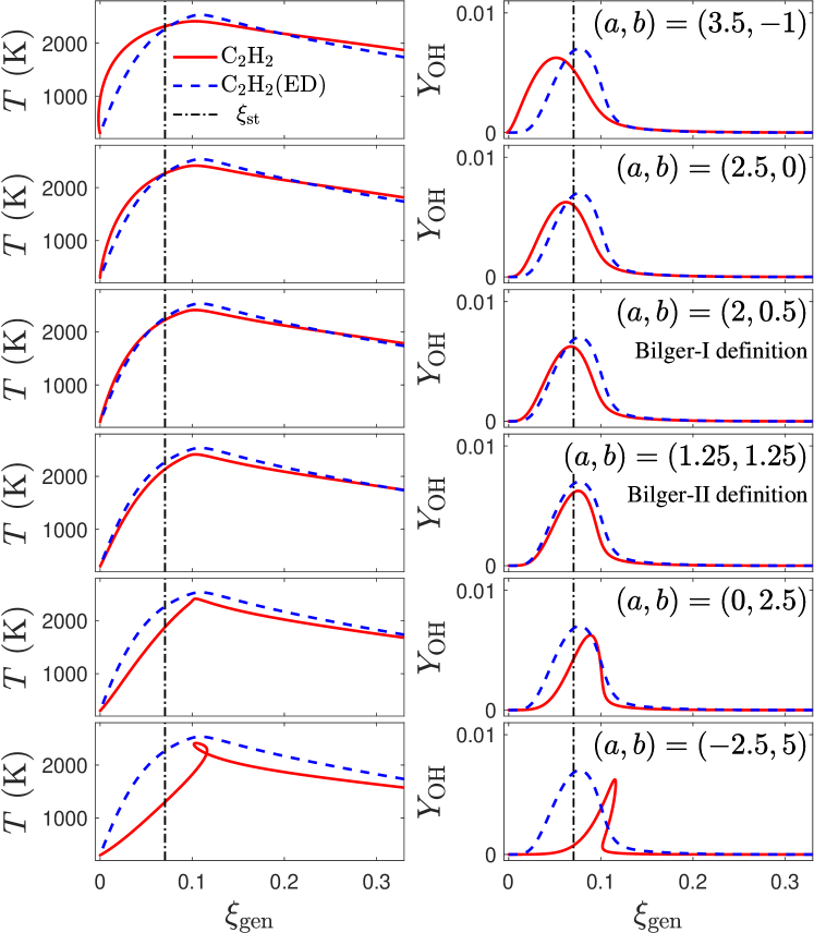
Figure 2: The profiles of the temperature $T\ (\mathrm{K})$ and the OH mass fraction $Y_{\mathrm{OH}}$ against the generalized mixture fraction $\xi_{\mathrm{gen}}$ with the different values of $(a,b)$ in the non-premixed $\mathrm{C_{2}H_{2}}$-air opposed jet laminar flame with the strain rate $s=50\ \mathrm{s}^{-1}$. The vertical dash-dotted lines indicate the stoichiometric value $\xi_{\mathrm{st}}=0.0705$.

Figure 2 shows the profiles of the temperature $T\ (\mathrm{K})$ and the OH mass fraction $Y_{\mathrm{OH}}$ against the generalized mixture fraction $\xi_{\mathrm{gen}}$ with a few selected values of $(a,b)$ in the non-premixed $\mathrm{C_{2}H_{2}}$-air opposed jet laminar flame. The ED model results are used as a reference, shown as the dashed lines in Figure 2. Since the stoichiometric mixture fraction $\xi=\xi_{\mathrm{st}}$ generally cannot be used as a reliable indicator of the stoichiometric condition (flame front) when differential molecular diffusion is present, it is useful to define a flame front indicator $\xi_{\mathrm{F}}$ to measure the deviation of $\xi=\xi_{\mathrm{st}}$ from the actual stoichiometric condition. Typically, the peak locations of minor radicals occur near the flame front and hence can be used as a flame front indicator. In this work, we use three common radicals (OH, O, and H) that exist in all hydrocarbon fuel combustion and their average peak location as the indicator of the flame front. The performance of this flame front indicator, $\xi_{\mathrm{F}}$, is examined in B for two laminar opposed jet flames ($\mathrm{CH_{4}/H_{2}}$-air flame and $\mathrm{H_{2}/CO_{2}}$-air flame). For the C₂H₂-air flame in Figure 2, $\xi_{\mathrm{F,ED}}=0.077$ which is slightly larger than the stoichiometric condition $\xi_{\mathrm{st}}=0.0705$. We use this value $\xi_{\mathrm{F,ED}}=0.077$ from ED as a reference for the flame front location for the assessment of the different mixture fraction definitions. The ED model results with different $(a,b)$ in Figure 2 are identical, verifying that the different mixture fraction definitions are the same under the ED assumption. The values $(a,b)=(2,0.5)$ correspond to Bilger-I (the third row of Figure 2), and $(1.25,1.25)$ (obtained from equation (9) with $\mathcal{X}=1$ and $a/b=1$ for $\mathrm{C_{2}H_{2}}$) correspond to Bilger-II (the fourth row of Figure 2). Both definitions perform reasonably well with the relative error of matching $\xi_{\mathrm{F}}$ within 11% for Bilger-I ($\xi_{\mathrm{F}}=0.069$) and 1% for Bilger-II ($\xi_{\mathrm{F}}=0.076$). Bilger-II yields particularly good agreement of $\xi_{\mathrm{F}}$ with the ED model result for the case. It is worthwhile to point out that the effect of differential molecular diffusion is still present in the results including the major species in the $\mathrm{C_{2}H2_{2}}$ flame (results not shown) despite the good agreement of the flame front location with the ED model, i.e., the use of different mixture fraction definitions does not change the effect of differential molecular diffusion. Additional four cases are considered in Figure 2 with two of them having $a\times b=0$ and two of them having $a\times b<0$. Generally, when $a$ or $b$ approaches zero, the deviation of $\xi_{\mathrm{F}}$ from $\xi_{\mathrm{F,ED}}$ becomes larger. When either $a<0$ or $b<0$, the deviation becomes even larger and the mixture fraction is not monotonic anymore. It is thus generally desired to have $a$ and $b$ positive or at least not significantly below zero. Requiring $a>0$ in equation (9), we can find that $b$ must be $b<2/\mathcal{X}+1/2$. Thus, the positivity of both $a$ and $b$ requires $b\in(0,2/\mathcal{X}+1/2)$. Substituting $b>0$ into equation (9), we obtain that $a<2+\mathcal{X}/2$, and hence the range of values that $a$ can take is $a\in(0,2+\mathcal{X}/2)$. For the current fuel $\mathrm{C_{2}H_{2}}$, $\mathcal{X}=1$, and hence $a\in(0,2.5)$ and $b\in(0,2.5)$. These ranges can be easily determined for any fuel $\{\mathrm{CH}_{\mathcal{X}}\}$ and can be used to guide the choice of the value $b$ for defining the mixture fraction.

Figure 3: The variations of the flame front location in the mixture fraction space $\xi_{\mathrm{F}}$ (solid lines) against the free parameter $b$ in the generalized mixture fraction $\xi_{\mathrm{gen}}$ in twelve different fuel-air non-premixed opposed jet flames. (The mole ratio is 1:1 for the fuel/H₂ mixture cases; Dashed lines: $\xi_{\mathrm{F,ED}}$ from ED; Dash-dotted lines: the stoichiometric values $\xi_{\mathrm{st}}$; Diamond symbols: Bilger-I; Pentagram symbols: Bilger-II; Circles: the intersection between solid lines and dashed lines; The values of $b$ shown in the figure correspond to the locations of the circles; The shaded areas cover the condition of either $a<0$ or $b<0$.)

Figure 3 further examines the variations of $\xi_{\mathrm{F}}$ against a continuous variation of the free parameter $b$ in $\xi_{\mathrm{gen}}$ for the $\mathrm{C_{2}H_{2}}$-air flame as well as eleven other opposed jet flames with fuels $\mathrm{CH_{4}}$, $\mathrm{C_{2}H_{4}}$, $\mathrm{C_{3}H_{6}}$, $\mathrm{C_{3}H_{8}}$, $\mathrm{C_{4}H_{10}}$, and these fuels mixed with $\mathrm{H_{2}}$ at the mole ratio of 1:1. The strain rate of the opposed jet flames is specified to be $s=50\ \mathrm{s}^{-1}$ and the USC-Mech II mechanism [24] is used for all the different fuel cases. For the $\mathrm{C_{2}H_{2}}$ flame case (the first plot in the second row in Figure 3), we see that $\xi_{\mathrm{F}}$ varies linearly against $b$. The values of $\xi_{\mathrm{st}}$ and $\xi_{\mathrm{F,ED}}$ are close to each other. Increasing the value of $b$ leads to an increase in the calculated $\xi_{\mathrm{F}}$. Both Bilger-I (diamond) and Bilger-II (pentagram) yield slightly smaller $\xi_{\mathrm{F}}$ when compared with $\xi_{\mathrm{F,ED}}$. It is found that the value $b\approx 1.36$ yields a perfect match with $\xi_{\mathrm{F,ED}}$. For all the other fuels and fuel mixtures in Figure 3, similar observations can be made. For fuel $\mathrm{CH_{4}}$, Bilger-I and Bilger-II are identical with $b=0.5$, and $b\approx 1.29$ is found to yield a perfect match with $\xi_{\mathrm{F,ED}}$. Bilger-II is found to match $\xi_{\mathrm{F,ED}}$ slightly better than Bilger-I in Figure 3 in most of the flames except the $\mathrm{CH_{4}}$ or $\mathrm{CH_{4}/H_{2}}$ flame.

The values of $b$ that yield a perfect match with $\xi_{\mathrm{F,ED}}$ are generally different for the different flames. In some cases, these values of $b$ are in the shaded areas ($a<0$ or $b<0$) like the CH₄ flame, which generally are not advised.

Some of the fuel or fuel mixtures examined in Figure 3 belong to the same fuel type, e.g., $\mathrm{C_{2}H_{2}/H_{2}}$, $\mathrm{C_{2}H_{4}}$, and $\mathrm{C_{3}H_{6}}$ are in the fuel type $\{\mathrm{CH_{2}}\}$, $\mathrm{C_{2}H_{4}/H_{2}}$ and $\mathrm{C_{4}H_{10}/H_{2}}$ are in $\{\mathrm{CH_{3}}\}$, and $\mathrm{C_{3}H_{6}/H_{2}}$ and $\mathrm{C_{3}H_{8}}$ are in $\{\mathrm{CH_{8/3}}\}$. The generalized mixture fraction definitions for the different fuels of the same type are identical. It is thus interesting to compare the performance of the same mixture fraction definition in the different fuel mixtures of the same fuel type. Taking the fuel type $\{\mathrm{CH_{2}}\}$ ($\mathrm{C_{2}H_{2}/H_{2}}$, $\mathrm{C_{2}H_{4}}$, and $\mathrm{C_{3}H_{6}}$) as an example, the values of $b$ are the same for Bilger-I ($b=0.5$) and Bilger-II ($b=0.75$). The stoichiometric mixture fraction value is also the same for this group of fuels, $\xi_{\mathrm{st}}=0.0637$. The difference is in the yielded flame front locations $\xi_{\mathrm{F}}$ based on the different mixture fraction definitions. One particular difference is the value of $b$ that produces a perfect match between $\xi_{\mathrm{F}}$ and $\xi_{\mathrm{F,ED}}$, $b\approx 0.67$, 1.18, and 1.31 for $\mathrm{C_{2}H_{2}/H_{2}}$, $\mathrm{C_{2}H_{4}}$, and $\mathrm{C_{3}H_{6}}$, respectively. This indicates the performance difference of the same mixture fraction definitions for different fuels (that belong to the same fule type). The difference is expected due to the different levels of differential molecular diffusion in the different flames.

Table 1: The sensitivity of the flame front location $\xi_{\mathrm{F}}$ from the generalized Bilger mixture fraction with respect to the free parameter $b$ expressed in terms of the values of the slope $\mathrm{d}\xi_{\mathrm{F}}/\mathrm{d}b$ for the different fuel types ($\{\mathrm{CH_{\mathcal{X}}}\}$ and $\{\mathrm{CH_{\mathcal{X}}O_{\mathcal{Y}}}\}$). The mole ratio of the fuel components is 1:1 for the fuel mixtures except for $\mathrm{H_{2}/CO_{2}}$ (36%/64% mole ratio) and $\mathrm{CH_{4}}$/air (1:3 mole ratio).

Fuel $\{\mathrm{CH_{\mathcal{X}}}\}$	$\mathrm{d}\xi_{\mathrm{F}}/\mathrm{d}b$		Fuel $\{\mathrm{CH_{\mathcal{X}}O_{\mathcal{Y}}}\}$	$\mathrm{d}\xi_{\mathrm{F}}/\mathrm{d}b$
CH4	0.0054		H2/CO2	0.3236
CH4/H2	0.0409		CH4/air	-0.0310
C2H2	0.0099		H2/CO	0.1577
C2H2/H2	0.0541		CH4/CO2	0.0197
C2H4	0.0084		CH4/H2O	0.0013
C2H4/H2	0.0507		CH4/CO	0.0085
C3H6	0.0071		C2H2/CO2	0.0021
C3H6/H2	0.0488		C2H5OH/CO2	-0.0024
C3H8	0.0079		C2H2/CO	0.0032
C3H8/H2	0.0473		C2H5OH/CO	-0.0065
C4H10	0.0075		C2H5OH	0.0189
C4H10/H2	0.0467		C2H5OH/H2	0.0310

The linearity of the flame front $\xi_{\mathrm{F}}$ against $b$ is observed evidently in all the different flames in Figure 3. This linearity can indeed be verified analytically as shown in C. The slope of the $\xi_{\mathrm{F}}$ curves, $\mathrm{d}\xi_{\mathrm{F}}/\mathrm{d}b$, in Figure 3 indicates the sensitivity of the generalized mixture fraction definitions to the parameter $b$. It also reflects the effect of differential molecular diffusion. In the limit of equal diffusion, such sensitivity disappears, $\mathrm{d}\xi_{\mathrm{F}}/\mathrm{d}b=0$. Table 1 summarizes the slope values $\mathrm{d}\xi_{\mathrm{F}}/\mathrm{d}b$ for the different fuels examined in Figure 3 (for the fuel type $\{\mathrm{CH_{\mathcal{X}}}\}$). For the pure hydrocarbon fuels (without $\mathrm{H_{2}}$ addition), the slope values are relatively low ($\mathrm{d}\xi_{\mathrm{F}}/\mathrm{d}b<0.01$), indicating relatively low sensitivity. Among the examined, $\mathrm{C_{2}H_{2}}$ shows the highest sensitivity ($\mathrm{d}\xi_{\mathrm{F}}/\mathrm{d}b=0.0099$) followed by $\mathrm{C_{2}H_{4}}$ ($\mathrm{d}\xi_{\mathrm{F}}/\mathrm{d}b=0.0084$), and $\mathrm{CH_{4}}$ shows the least sensitivity ($\mathrm{d}\xi_{\mathrm{F}}/\mathrm{d}b=0.0054$). The addition of $\mathrm{H_{2}}$ to the hydrocarbon fuels enhances the sensitivity significantly and increases the slope values by approximately one order of magnitude to $\mathrm{d}\xi_{\mathrm{F}}/\mathrm{d}b\approx 0.05$.

In summary, a new class of generalized Bilger mixture fraction definitions is introduced for hydrocarbon fuels or fuel mixtures in the form of $\{\mathrm{CH}_{\mathcal{X}}\}$. Both Bilger-I and Bilger-II belong to this class of definitions. The performance of this class of mixture fraction definitions in terms of stoichiometry preservation is examined and compared in twelve laminar non-premixed opposed jet flames with different fuels and fuel mixtures. Overall, we see similar performance of Bilger-I and Bilger-II with only some slight performance differences depending on the case. The ranges of the free parameter $b$ that can lead to negative values of $a$ and $b$ are identified for different fuels and are generally not advised. The sensitivity of the generalized mixture fraction definitions to the variation of the free parameter $b$ is also examined.

4 Mixture fraction for the fuel type $\{\mathrm{CH_{\mathcal{X}}O_{\mathcal{Y}}}\}$

4.1 Generalized mixture fraction definitions for $\{\mathrm{CH_{\mathcal{X}}O_{\mathcal{Y}}}\}$

We next extend the generalized mixture fraction definitions in Section 3 to fuel cases containing the oxygen element like the fuel $\mathrm{C_{2}H_{5}OH}$ or fuel mixture $\mathrm{CH_{4}/CO_{2}}$. We write the fuel in a general form as $\{\mathrm{CH_{\mathcal{X}}O_{\mathcal{Y}}}\}$ which can be either a pure substance or a mixture. The corresponding pseudo global reaction is written as,

$$\{\mathrm{CH_{\mathcal{X}}O_{\mathcal{Y}}}\}+\frac{4+\mathcal{X}-2\mathcal{Y}}{4}\times\mathrm{O_{2}}\rightarrow\mathrm{CO_{2}}+\frac{\mathcal{X}}{2}\times\mathrm{H_{2}O}.$$ (13)

Following the derivation in Section 3.2, we can derive a class of generalized Bilger mixture fraction for $\{\mathrm{CH_{\mathcal{X}}O_{\mathcal{Y}}}\}$-air combustion too.

we found that the element specific mole numbers at the stoichiometric condition for $\{\mathrm{CH_{\mathcal{X}}O_{\mathcal{Y}}}\}$ are the same as those for $\{\mathrm{CH_{\mathcal{X}}}\}$ in equation (7). Substituting equation (7) into equation (4), we obtain the same equation (8) and hence the same relation for the parameters $a$ and $b$ in equation (9). Thus, the class of the general mixture fraction definitions for $\{\mathrm{CH_{\mathcal{X}}}\}$ derived in Section 3.2 is also applicable to $\{\mathrm{CH_{\mathcal{X}}O_{\mathcal{Y}}}\}$. It is interesting to notice that the oxygen element number $\mathcal{Y}$ in $\{\mathrm{CH_{\mathcal{X}}O_{\mathcal{Y}}}\}$ does not appear in the generalized mixture fraction definitions.

The Bilger-I definition in equation (1) can be extended straightforwardly to fuel $\{\mathrm{CH_{\mathcal{X}}O_{\mathcal{Y}}}\}$ as,

$$\xi_{\mathrm{Bilger\text{-}I}}=\frac{\frac{2(Y_{\mathrm{C}}-Y_{\mathrm{C,o}})}{W_{\mathrm{C}}}+\frac{Y_{\mathrm{H}}-Y_{\mathrm{H,o}}}{2W_{\mathrm{H}}}-\frac{Y_{\mathrm{O}}-Y_{\mathrm{O,o}}}{W_{\mathrm{O}}}}{\frac{2(Y_{\mathrm{C,f}}-Y_{\mathrm{C,o}})}{W_{\mathrm{C}}}+\frac{Y_{\mathrm{H,f}}-Y_{\mathrm{H,o}}}{2W_{\mathrm{H}}}-\frac{Y_{\mathrm{O,f}}-Y_{\mathrm{O,o}}}{W_{\mathrm{O}}}}.$$ (14)

It can be readily verified that this definition belongs to the generalized Bilger mixture fraction in equations (3) and (10) with $(a,b)=(2,1/2)$. The definition has fixed coefficients and does not depend on the fuel’s chemical composition. The use of the extended Bilger-I is extensive in the literature, e.g., [13, 25]. It is worthwhile to mention a revised version of Bilger-I which has the O element removed since it has been used in the widely studied Sandia flames [26, 27]. The removal is due to a different consideration to reduce the effect of experimental noise on the calculated mixture fraction [26]. The revised definition does not belong to the general mixture fraction definition. The effect of differential molecular diffusion in the Sandia flames like the Sandia piloted flames D, E, and F [26] is relatively small and is limited to the near field, so the use of the revised Bilger-I (without the stoichiometry preservation property) is not expected to be an issue.

The extension of Bilger-II in equation (2) to $\{\mathrm{CH_{\mathcal{X}}O_{\mathcal{Y}}}\}$ is straightforward too as [15],

$$\xi_{\mathrm{Bilger\text{-}II}}=\frac{\frac{Y_{\mathrm{C}}-Y_{\mathrm{C,o}}}{mW_{\mathrm{C}}}+\frac{Y_{\mathrm{H}}-Y_{\mathrm{H,o}}}{nW_{\mathrm{H}}}-\frac{Y_{\mathrm{O}}-Y_{\mathrm{O,o}}}{(m+0.25n)W_{\mathrm{O}}}}{\frac{Y_{\mathrm{C,f}}-Y_{\mathrm{C,o}}}{mW_{\mathrm{C}}}+\frac{Y_{\mathrm{H,f}}-Y_{\mathrm{H,o}}}{nW_{\mathrm{H}}}-\frac{Y_{\mathrm{O,f}}-Y_{\mathrm{O,o}}}{(m+0.25n)W_{\mathrm{O}}}},$$ (15)

which is written for a fuel that contains $m$ carbon element and $n$ hydrogen element ($m/n=\mathcal{X}$) as in equation (2). It can be verified that this definition belongs to the class of generalized definition in equations (3) and (10) with $(a,b)=\left((4+\mathcal{X})/4,(4+\mathcal{X})/4\mathcal{X}\right)$ (the same as equation (12) for $\{\mathrm{CH_{\mathcal{X}}}\}$). The definition has fuel-dependent coefficients and hence is different for different fuels. The oxygen element number $\mathcal{Y}$ does not appear in the formulation and hence the definition is the same as that for $\{\mathrm{CH_{\mathcal{X}}}\}$.

4.2 Examination of mixture fraction definitions for $\{\mathrm{CH_{\mathcal{X}}O_{\mathcal{Y}}}\}$ in opposed jet laminar flames

Figure 4: The profiles of the temperature $T\ (\mathrm{K})$ and the OH mass fraction $Y_{\mathrm{OH}}$ against the generalized mixture fraction $\xi_{\mathrm{gen}}$ with the different values of $(a,b)$ in the non-premixed $\mathrm{H_{2}/CO_{2}}$-air opposed jet laminar flame with the strain rate $s=50\ \mathrm{s}^{-1}$. The vertical dash-dotted lines are the stoichiometric value $\xi_{\mathrm{st}}=0.539$.

To compare the different mixture fraction definitions for $\{\mathrm{CH_{\mathcal{X}}O_{\mathcal{Y}}}\}$, we consider a non-premixed opposed jet laminar flame with the fuel $\mathrm{H_{2}/CO_{2}}$ (36%/64% mole ratio following the experimental configurations in a study of differential molecular diffusion in a $\mathrm{H_{2}/CO_{2}}$ jet flame [28]) and air at $s=50\ \mathrm{s}^{-1}$. The OPPDIF [23] calculations are performed with the USC-Mech II [24]. The effect of differential molecular diffusion in this flame is severe, and hence it is useful to choose this flame case to demonstrate the difference between different mixture fraction definitions. Figure 4 shows the profiles of the temperature $T\ (\mathrm{K})$ and the OH mass fraction $Y_{\mathrm{OH}}$ against the generalized mixture fraction $\xi_{\mathrm{gen}}$ in equations (3) and (10) with a few selected values of $(a,b)$ in the $\mathrm{H_{2}/CO_{2}}$-air flame.

Overall, the Bilger-I definition (the fourth row in Figure 4) performs the best for this case with the predicted location $\xi_{\mathrm{F}}=0.518$ slightly different from $\xi_{\mathrm{F,ED}}=0.546$ (or $\xi_{\mathrm{st}}=0.539$), and all the other definitions, including Bilger-II, perform poorly in Figure 4.

The particular definitions in the generalized mixture fraction definition with $b\leq 0.25$ (the first three rows in Figure 4) including the case of $b=0.0$ yields some significant underprediction of $\xi_{\mathrm{F}}$. The Bilger-II definition performs poorly too for the H₂/CO₂-air flame with $\xi_{\mathrm{F}}=0.724$ (the fifth row in Figure 4). It yields a significant over-prediction of $\xi_{\mathrm{F}}$ and a non-monotonic variation of the mixture fraction in the physical space even though it belongs to the generalized mixture fraction. It shows the performance difference between the different mixture fraction definitions even from the same class of generalized Bilger mixture fraction definitions. The case of $a=0$ (the sixth row of Figure 4) performs poorly as well in the figure. Although there is a class of mixture fraction definitions for $\{\mathrm{CH_{\mathcal{X}}O_{\mathcal{Y}}}\}$, different definitions do not perform equally, and it is useful to identify a common choice that suits a wide range of applications. In this regard, the Bilger-I definition seems a preferred choice since it performs overall well so far. The Bilger-II definition can sometimes yield relatively poor performance like in the current H₂/CO₂-air flame.

Figure 5: The variations of the flame front location in the mixture fraction space $\xi_{\mathrm{F}}$ (solid lines) against the free parameter $b$ in the generalized mixture fraction $\xi_{\mathrm{gen}}$ in twelve different fuel-air non-premixed opposed jet flames. (The mole ratio is 1:1 for the fuel mixture cases except for $\mathrm{H_{2}/CO_{2}}$ (36%/64% mole ratio) and $\mathrm{CH_{4}}$/air (1:3 mole ratio); Dashed lines: $\xi_{\mathrm{F,ED}}$ from ED; Dash-dotted lines: the stoichiometric values $\xi_{\mathrm{st}}$; Diamond symbols: Bilger-I; Pentagram symbols: Bilger-II; Circles: the intersection between solid lines and dashed lines; The values of $b$ shown in the figure correspond to the locations of the circles; The shaded areas cover the condition of either $a<0$ or $b<0$.)

Figure 5 further examines the variations of $\xi_{\mathrm{F}}$ against the free parameter $b$ for twelve different fuels and fuel mixtures: $\mathrm{H_{2}/CO_{2}}$ (same as in Figure 4), $\mathrm{CH_{4}}$-air (mole ratio of 1:3 following the Sandia piloted jet flame condition [21]), $\mathrm{H_{2}/CO}$ (mole ratio of 1:1 for this and all the following fuel mixtures), $\mathrm{CH_{4}/CO_{2}}$, $\mathrm{CH_{4}/H_{2}O}$, $\mathrm{CH_{4}/CO}$, $\mathrm{C_{2}H_{2}/CO_{2}}$, $\mathrm{C_{2}H_{2}/CO}$, $\mathrm{C_{2}H_{5}OH}$, $\mathrm{C_{2}H_{5}OH/CO_{2}}$, $\mathrm{C_{2}H_{5}OH/CO}$, and $\mathrm{C_{2}H_{5}OH/H_{2}}$. The OPPDIF [23] calculations are performed with the USC-Mech II [24] except for the fuels that contain C₂H₅OH for which the San Diego Mechanism [29] is used. In all of these flames, the air is used as the oxidizer. Overall, we do not see significant sensitivity of the generalized mixture fraction to the variation of $b$ as long as $b\in(0,2/\mathcal{X}+1/2)$ (to ensure positive $a$ and $b$ as discussed in Section 3.3) except in the $\mathrm{H_{2}/CO_{2}}$-air and $\mathrm{H_{2}/CO}$-air flames. The strong sensitivity has already been seen in the $\mathrm{H_{2}/CO_{2}}$-air flame in Figure 4. It is expected to be related to the strong differential molecular diffusion effect in these two flames that causes a substantial deviation of the stoichiometric location from the ED limit. In the $\mathrm{H_{2}/CO_{2}}$-air flame, the Bilger-I definition performs well since $b=0.5$ in equation (11) is close to the perfect value of $b\approx 0.60$ (that yields a perfect match of $\xi_{\mathrm{F}}$ with $\xi_{\mathrm{F,ED}}$). The value of $b$ in Bilger-II is $b=1.14$ based on equation (12) which is almost twice the perfect value $b\approx 0.59$ and hence yields a significant deviation of $\xi_{\mathrm{F}}$ from $\xi_{\mathrm{F,ED}}$. In the $\mathrm{H_{2}/CO}$-air flame, Bilger-I and Bilger-II both perform well largely because the values of $b$, $b=0.5$ for Bilger-I and $b=0.75$ for Bilger-II, are close to the perfect value $b\approx 0.68$ shown in the figure. For all the other flames in Figure 5, all mixture fraction definitions including the particular solutions in the generalized mixture fraction with $b\in(0,2/\mathcal{X}+1/2)$ perform reasonably. The effect of differential molecular diffusion in those flames is not expected to be as profound as in the $\mathrm{H_{2}/CO_{2}}$-air flame or the $\mathrm{H_{2}/CO}$-air flame. It is useful to remind us that when the effect of differential molecular diffusion reduces and reaches the limit of ED, all mixture fraction definitions become identical.

Among the different fuel cases in Figure 5, five cases ($\mathrm{H_{2}/CO}$, $\mathrm{CH_{4}/CO_{2}}$, $\mathrm{CH_{4}/CO}$, $\mathrm{C_{2}H_{5}OH/CO_{2}}$, and $\mathrm{C_{2}H_{5}OH/CO}$) belong to the fuel type $\{\mathrm{CH_{2}O_{\mathcal{Y}}}\}$ and have the same generalized mixture fraction definitions since the value of $\mathcal{Y}$ does not appear in the general definition in equations (3) and (10). The generalized mixture fraction definitions perform differently in these different fuel cases and yield different values of $b$ to match $\xi_{\mathrm{F}}$ with $\xi_{\mathrm{F,ED}}$, $b\approx 0.68$, 1.00, 1.62, -4.68, -0.27 for $\mathrm{H_{2}/CO}$, $\mathrm{CH_{4}/CO_{2}}$, $\mathrm{CH_{4}/CO}$, $\mathrm{C_{2}H_{5}OH/CO_{2}}$, and $\mathrm{C_{2}H_{5}OH/CO}$, respectively. The fuel mixtures $\mathrm{C_{2}H_{2}/CO2}$ and $\mathrm{C_{2}H_{2}/CO}$ share the same mixture fraction definitions too. The cases of $\mathrm{CH_{4}/air}$ and $\mathrm{C_{2}H_{5}OH/H_{2}}$ have the same generalized mixture fraction definitions as well as the same definitions for Bilger-I and Bilger-II since $\mathcal{X}=4$ (the diamond (Bilger-I) and pentagram (Bilger-II) symbols overlap with each other in Figure 5 for the two fuels).

The slope values, $\mathrm{d}\xi_{\mathrm{F}}/\mathrm{d}b$, for the different fuel cases in Figure 5 are collected in Table 1 to indicate the sensitivity of the predicted flame front location $\xi_{\mathrm{F}}$ to the variation of the free parameter $b$ in the generalized mixture fraction. The blending of $\mathrm{H_{2}}$ in a fuel generally increases the sensitivity (with $\mathrm{d}\xi_{\mathrm{F}}/\mathrm{d}b>0.01$). The highest sensitivity is seen in the $\mathrm{H_{2}/CO_{2}}$ ($\mathrm{d}\xi_{\mathrm{F}}/\mathrm{d}b=0.3236$) and $\mathrm{H_{2}/CO}$ ($\mathrm{d}\xi_{\mathrm{F}}/\mathrm{d}b=0.1577$) flames. For pure fuels (without $\mathrm{H_{2}}$), generally the sensitivity is relatively small as it is seen in the fuel $\{\mathrm{CH}_{\mathcal{X}}\}$. A few exceptions exist in the $\mathrm{CH_{4}/air}$, $\mathrm{CH_{4}/CO_{2}}$, and $\mathrm{C_{2}H_{5}OH}$ flames where relatively high sensitivity is seen, say $\mathrm{d}\xi_{\mathrm{F}}/\mathrm{d}b>0.01$. It is also observed that the slope $\mathrm{d}\xi_{\mathrm{F}}/\mathrm{d}b$ is positive for most of the fuel cases in Table 1 except in the $\mathrm{CH_{4}/air}$, $\mathrm{C_{2}H_{5}OH/CO_{2}}$, and $\mathrm{C_{2}H_{5}OH/CO}$ flames where a negative slope is observed.

In summary, we discussed a class of generalized mixture fraction definitions for the fuel type $\{\mathrm{CH_{\mathcal{X}}O_{\mathcal{Y}}}\}$. It is found that the general definition is the same form as that for $\{\mathrm{CH_{\mathcal{X}}}\}$. Both the Bilger-I and Bilger-II definitions are seen to belong to this class when properly extended to $\{\mathrm{CH_{\mathcal{X}}O_{\mathcal{Y}}}\}$.

In twelve opposed jet laminar flames with different fuels, we found that the Bilger-I definition performs reasonably well for all the test cases considered. This supports the decades of use of Bilger-I in numerious studies. Bilger-II can sometimes yield poor results, e.g. in the $\mathrm{H_{2}/CO_{2}}$-air flames when the effect of differential molecular diffusion is severe.

5 “Optimal” mixture fraction definitions

Given the existence of many mixture fraction definitions that are similar to Bilger’s and the observed performance difference of the different definitions, it is intriguing to examine the feasibility of identifying an optimal mixture fraction among the class of definitions. Based on the discussions above, it is clear that a universally optimal mixture fraction definition (with a fixed value of $b$ in the general definition) that works for all different fuels does not exist. Even under the same fuel and oxidizer configuration in an opposed jet flame but with different strain rates, the perfect value of the free parameter $b$ in the generalized mixture fraction definition is different. The concept of an “optimal” mixture fraction discussed here thus has some limitations. Nevertheless, it is still valuable to assess the feasibility of defining an “optimal” mixture fraction in some limited sense. In particular, we aim to seek an optimal mixture fraction definition that works for flames with the same fuel and oxidizer under different stretching conditions. We formulate the problem as a minimization problem, and the optimal solutions are discussed for several different flames in this section.

5.1 Minimization and cost function

Since the three desired properties of mixture fraction in Section 2 cannot be satisfied simultaneously by any definition. The goal of the minimization here is thus to minimize the deviation of a mixture fraction definition from all the desired properties. The cost function $C$ for the minimization can be designed as,

$$C=w_{\mathrm{S}}\cdot C_{\mathrm{S}}+w_{\mathrm{M}}\cdot C_{\mathrm{M}}+w_{\mathrm{B}}\cdot C_{\mathrm{B}},$$ (16)

that consists of three components. The first component $C_{\mathrm{S}}$ measures the deviation of the stoichiometric value of mixture fraction from the actual stoichiometric condition. The second component $C_{\mathrm{M}}$ checks the level of violation of monotonicity of a mixture fraction definition in the physical space. The third component $C_{\mathrm{B}}$ examines the boundedness violation. The coefficients $w_{\mathrm{S}}$, $w_{\mathrm{M}}$, and $w_{\mathrm{B}}$ in equation (16) are the relative weight of each component for the cost function. Equal weight ($w_{\mathrm{S}}=w_{\mathrm{M}}=w_{\mathrm{B}}=1$) has been used in this work. The weights can be easily adjusted if needed. The focus here is to examine the feasibility of identifying optimal mixture fraction definitions so equal weights are used for simplicity. Different weights can be used if more weight is desired for a component of the cost function based on the need of a particular application. It can be argued that a monotonic mixture fraction can guarantee the boundedness so the inclusion of $C_{\mathrm{B}}$ in the cost function is redundant. The consideration here is that the monotonicity violation can occur near the boundaries or away from the boundaries (see examples in figure 4). This difference is not included in the cost $C_{\mathrm{M}}$. The additional cost $C_{\mathrm{B}}$ puts more weight on the monotonicity violation near the boundaries. The details of defining each component of the cost function are discussed in Sections 5.2-5.4 below.

The cost function for the mixture fraction optimization is calculated based on the numerical solutions of opposed jet laminar non-premixed flames under different stretching conditions. We use $\xi_{i,m}$ to denote the calculated mixture fraction at the $i$-th grid location $x_{i}$ for the $m$-th strain rate $s_{m}$. The number of grid points $n_{x}$ used for the simulations is adaptively determined by OPPDIF. For all the simulation cases below, more than $n_{x}=800$ grid points are used by OPPDIF to ensure numerical accuracy. A number of strain rates $n_{s}$ is used to cover different stretching conditions ranging from the lowest stretching $s=1\ \mathrm{s}^{-1}$ to the extinction limit $s_{\mathrm{e}}$. For different fuel/oxidizer cases, the extinction limit $s_{\mathrm{e}}$ has different values. For all the simulation cases, we use at least $n_{s}=50$ different strain rate values to adequately represent the effect of different levels of stretching on the flames.

5.2 Preservation of stoichiometric condition

In Sections 3.3 and 4.2, the value of $\xi_{\mathrm{F,ED}}$ from the ED model under the same strain rate is used as a reference to examine the deviation of the stoichiometric mixture fraction from the actual stoichiometric condition. Here, a slight modification is introduced to measure the deviation. The flame front location can vary noticeably when the strain rate changes as illustrated in Figure 11 in B. The flame location near the extinction limit can be different from that far from extinction. The extinction limits can be significantly different with or without differential molecular diffusion. For example, the extinction limit of the H₂/CO₂-air opposed jet flame is $s_{\mathrm{e}}=1649\ s^{-1}$ when the mixture-averaged molecular diffusion model is used, while that limit with ED is only $s_{\mathrm{e}}=686\ s^{-1}$. For a high strain rate ($s>686\ s^{-1}$), there is not a valid value of $\xi_{\mathrm{F,ED}}$ as a reference because of extinction. Hence, we introduce a normalized strain rate $\theta=s/s_{\mathrm{e}}$ so that the flame front location under different strain rates with or without differential molecular diffusion can be measured under similar relative departure from extinction. The value of $\xi_{\mathrm{F,ED}}$ from the ED model under the same normalized strain rate $\theta$ is then used as a reference for minimizing the deviation of the value of $\xi_{\mathrm{F}}$ from $\xi_{\mathrm{F,ED}}$ when differential molecular diffusion is considered.

With the above modification, the cost function $C_{\mathrm{S}}$ for minimizing the deviation of mixture fraction $\xi_{\mathrm{F}}$ from the stoichiometric condition is written as,

$$C_{\mathrm{S}}=\left[\frac{1}{n_{s}}\sum_{m=1}^{n_{s}}\left(\xi_{\mathrm{F},m}-\xi_{\mathrm{F,ED}}(\theta_{m})\right)^{2}\right]^{1/2},$$ (17)

where $\xi_{\mathrm{F},m}$ is the flame front location for a mixture fraction definition measured based on the approach in B as the average of the peak locations of the three common radicals corresponding to the $m$-th strain rate $\theta_{m}=s_{m}/s_{\mathrm{e}}$, and $\xi_{\mathrm{F,ED}}(\theta_{m})$ is the flame location computed with the ED model under the same normalized strain rate $\theta_{m}=s_{m,\mathrm{ED}}/s_{\mathrm{e,ED}}$.

5.3 Monotonicity of mixture fraction

The monotonicity of a mixture fraction definition is examined by integrating in the physical space the gradient of the mixture fraction that is opposite from the overall variation of the mixture fraction. The cost function $C_{\mathrm{M}}$ to evaluate the violation of monotonicity based on the numerical solutions of the opposed jet flames is written discretely as,

$$C_{\mathrm{M}}=\left[\frac{1}{n_{s}}\sum_{m=1}^{n_{s}}\sum_{i=1}^{n_{x}-1}\left(\min\left(\frac{\xi_{i+1,m}-\xi_{i,m}}{\xi_{n_{x},m}-\xi_{1,m}},0\right)\right)^{2}\right]^{1/2},$$ (18)

where $\xi_{i,m}$ is the computed mixture fraction at the $i$-th grid point from the $m$-th strain rate, $\xi_{n_{x},m}$ and $\xi_{1,m}$ represent the mixture fraction values on the boundaries (either 0 or 1), and the minimum function ensures that only those points violating the monotonicity are included in the cost function.

5.4 Boundedness of mixture fraction

The cost function $C_{\mathrm{B}}$ to assess the boundedness violation of a mixture fraction definition is written as,

$$C_{\mathrm{B}}=\left[\frac{1}{n_{s}}\sum_{m=1}^{n_{s}}\frac{\sum_{i=1}^{n_{x}}\left(J_{i,m}\cdot\left(\left[\max(\xi_{i,m}-1,0)\right]^{2}+\left[\min(\xi_{i,m},0)\right]^{2}\right)\right)}{\sum_{i=1}^{n_{x}}J_{i,m}}\right]^{1/2},$$ (19)

where $J_{i,m}$ is used to ensure that only points violating boundedness are included in the cost function calculation and is defined as,

$$J_{i,m}=\left\{\begin{array}[]{ll}0,&\mathrm{if}\ \ 0\leq\xi_{i,m}\leq 1\\ 1,&\mathrm{otherwise}\end{array}\right..$$ (20)

5.5 Cost function minimization and optimal mixture fraction

Figure 6: The profile of the cost function $C$ against the free parameter $b$ for the generalized mixture fraction in equations (3) and (10) in the H₂/CO₂-air opposed jet flames with different strain rates.

The minimization is carried out with the above-defined cost function $C$ in equation (16). With the generalized mixture fraction $\xi_{\mathrm{gen}}$ in equations (3) and (10), the cost $C$ becomes a function of the free parameter $b$ only. A typical shape of the cost function against $b$ is shown in Figure 6 for the H₂/CO₂-air opposed jet flames. The cost function has a global minimum at about $b\approx 0.676$. Other fuel flames have similar cost function profiles with the global minimum occurring at different values of $b$. The minimization problem can be solved easily by finding the solution to $dC/db=0$.

Table 2: Optimized mixture fraction definitions for the different fuel types ($\{\mathrm{CH_{\mathcal{X}}}\}$ and $\{\mathrm{CH_{\mathcal{X}}O_{\mathcal{Y}}}\}$) and their comparison with the Bilger-I and Bilger-II definitions. The parameters $a$ and $b$ are related by equation (9) in the generalized mixture fraction in equations (3) and (10). The cost function $C$ is computed based on equation (16). The “Optimal” definitions correspond to the minimum of the cost function $C$. The mole ratio of the fuel components is 1:1 for the fuel mixtures except for $\mathrm{H_{2}/CO_{2}}$ (36%/64% mole ratio) and $\mathrm{CH_{4}}$/air (1:3 mole ratio).

Fuel $\{\mathrm{CH_{\mathcal{X}}}\}$	Optimal				Bilger-I				Bilger-II
or $\{\mathrm{CH_{\mathcal{X}}O_{\mathcal{Y}}}\}$	$a$	$b$	$C$		$a$	$b$	$C$		$a$	$b$	$C$
CH4	-0.0019	1.0005	0.0209		2.0000	0.5000	0.0303		2.0000	0.5000	0.0303
CH4/H2	1.3477	0.6087	0.0078		2.0000	0.5000	0.0331		2.5000	0.4167	0.0574
C2H2	1.2220	1.2780	0.0647		2.0000	0.5000	0.0771		1.2500	1.2500	0.0647
C2H2/H2	1.5234	0.7383	0.0332		2.0000	0.5000	0.0977		1.5000	0.7500	0.0335
C2H4	0.5124	1.2438	0.0337		2.0000	0.5000	0.0536		1.5000	0.7500	0.0437
C2H4/H2	1.5047	0.6651	0.0151		2.0000	0.5000	0.0602		1.7500	0.5833	0.0326
C3H6	0.5346	1.2327	0.0305		2.0000	0.5000	0.0481		1.5000	0.7500	0.0392
C3H6/H2	1.5840	0.6560	0.0132		2.0000	0.5000	0.0580		1.6667	0.6250	0.0173
C3H8	0.2980	1.1383	0.0219		2.0000	0.5000	0.0433		1.6667	0.6250	0.0372
C3H8/H2	1.5251	0.6425	0.0116		2.0000	0.5000	0.0519		1.8333	0.5500	0.0348
C4H10	-0.0154	1.3062	0.0174		2.0000	0.5000	0.0433		1.6250	0.6500	0.0367
C4H10/H2	1.5624	0.6459	0.0127		2.0000	0.5000	0.0533		1.7500	0.5833	0.0255
H2/CO2	1.8019	0.6760	0.1609		2.0000	0.5000	0.4513		1.2812	1.1389	1.2150
CH4/air	4.7378	-0.1845	0.0370		2.0000	0.5000	0.1739		2.0000	0.5000	0.1739
H2/CO	1.2194	0.8903	0.1815		2.0000	0.5000	0.5051		1.5000	0.7500	0.2483
CH4/CO2	1.1620	0.9190	0.0197		2.0000	0.5000	0.0688		1.5000	0.7500	0.0331
CH4/H2O	-3.7935	1.4656	0.0393		2.0000	0.5000	0.0467		2.5000	0.4167	0.0478
CH4/CO	-0.1330	1.5665	0.0394		2.0000	0.5000	0.0814		1.5000	0.7500	0.0674
C2H2/CO2	2.3901	-0.0851	0.1208		2.0000	0.5000	0.1217		1.1667	1.7500	0.1274
C2H5OH/CO2	3.8739	-0.4370	0.0423		2.0000	0.5000	0.0739		1.5000	0.7500	0.0939
C2H2/CO	2.6701	-0.5051	0.1067		2.0000	0.5000	0.1143		1.1667	1.7500	0.1419
C2H5OH/CO	3.0269	-0.0134	0.0146		2.0000	0.5000	0.0568		1.5000	0.7500	0.0854
C2H5OH	1.4521	0.6826	0.0284		2.0000	0.5000	0.0436		1.7500	0.5833	0.0344
C2H5OH/H2	1.2416	0.6896	0.0343		2.0000	0.5000	0.0581		2.0000	0.5000	0.0581

Table 2 summarizes the optimization results and their comparison with Bilger-I and Bilger-II for 24 different fuels and fuel mixtures. The optimal values of $b$ for the different fuels that minimize the cost function $C$ are shown in the table under the column “Optimal”. The values of $a$ are calculated from the corresponding values of $b$ by using equation (9). The minimum values of the cost function $C$ achieved with the optimal $b$ for the different fuels are shown in the table (under “Optimal”). The values of $a$ and $b$ and the cost function $C$ based on Bilger-I and Bilger-II are also shown in the table for comparison. The optimal values of $a$ and $b$ are found to be positive for most fuels with a few exceptions. The reduction of the cost function of the optimal mixture fraction is evident for some fuels when compared with Bilger-I and Bilger-II. The reduction is not uniform for the different fuels. For CH₄/H₂, CH₄/air, and C₂H₅OH/CO, the reduction of the cost function can reach above 70%. For C₂H₂, C₂H₂/H₂, H₂/CO, and C₂H₂/CO₂, the reduction is negligibly small since the existing definitions are close to optimal. Other fuels have variable levels of reduction of the cost function for the optimal mixture fraction between 5% and 70% relative to the Bilger-I or Bilger-II definitions.

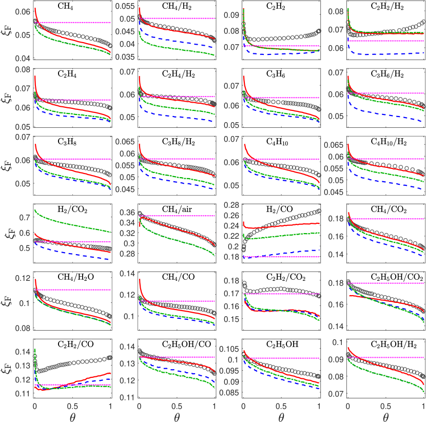
Figure 7: The profiles of the flame front locations in the mixture fraction space $\xi_{\mathrm{F}}$ against the normalized strain rate $\theta=s/s_{\mathrm{e}}$ for 24 different fuel flames. The circles show the ED model results as a reference, and the lines are the results with differential molecular diffusion and different mixture fraction definitions (solid red lines: “Optimal”; dashed blue lines: Bilger-I; dash-dotted green lines: Bilger-II; dotted magenta lines: stoichiometric mixture fraction $\xi_{\mathrm{st}}$).

The stoichiometry preservation of the optimized mixture fraction definitions is examined in Figure 7 for the different types of fuels. In the figure, the profiles of the flame front locations $\xi_{\mathrm{F}}$ (defined in B) are shown against the normalized strain rate $\theta=s/s_{\mathrm{e}}$ for the different fuel flames. The ED model results for $\xi_{\mathrm{F,ED}}$ shown as the circles are used as the target of the flame front for the optimization. The lines show the results with differential molecular diffusion and different mixture fraction definitions (the solid red lines: “Optimal”; dashed blue lines: Bilger-I; dash-dotted green lines: Bilger-II). The flame front locations vary noticeably when the strain rate is changed in the same fuel flame. All the different mixture fraction definitions capture this variation reasonably well. The optimized mixture fraction shows overall improvement relative to the Bilger-I or Bilger-II definitions among all the considered cases. For some flames, this improvement is significant (e.g., the CH₄/air flames), while for some other flames, the improvement is limited (e.g., the C₂H₂/CO₂ flames). The deviation of the flame fronts based on the optimized mixture fraction is still evident from the target for some flames, indicating the limitation of the optimal mixture fraction.

In summary, the concept of “optimal” mixture fraction is explored by minimizing the deviation of the generalized mixture fraction from the desired properties listed in Section 2. An optimization procedure is developed including a proper definition of the cost function. It is demonstrated among 24 different fuel configurations that the optimal mixture fraction shows overall better preservation of the stoichiometric condition while minimizing the cost function. The disadvantage of the optimal mixture fraction is that it requires a numerical optimization procedure to identify the optimal definition if a new fuel is encountered. The existing definitions based on Bilger’s are ready for use for any fuel given their simple definitions. For practical applications, the choice of the definition is better to be determined based on a specific user need and accuracy requirement. The study in this work provides necessary information and choices for making an informed decision on mixture fraction definitions.

6 Extension to other types of fuels

The introduced general approach in this work for deriving the mixture fraction definitions that preserve the stoichiometric condition is not limited to hydrocarbon fuels and can be readily extended to other fuel types like fuels that contain sulfur or nitrogen. Pure $\mathrm{H_{2}}$ is the simplest carbon-free fuel. It is not included in the general definition in equation (10) for $(a,b)$ but the corresponding Bilger mixture fraction can be easily found to be $(a,b)=(0,1/2)$ in equation (4), and it is unique. Ammonia ($\mathrm{NH_{3}}$) is another example of carbon-free fuel that has attracted attention in the industry due to climate concerns. To illustrate the extension of the approach to carbon-free fuels, we consider two general fuel types below: nitrogen hydride $\{\mathrm{NH}_{\mathcal{X}}\}$ and sulfur hydride $\{\mathrm{H}_{\mathcal{X}}\mathrm{S}\}$.

6.1 Generalized mixture fraction definitions for $\{\mathrm{NH_{\mathcal{X}}}\}$

For the fuel type $\{\mathrm{NH}_{\mathcal{X}}\}$, the general mixture fraction is defined in the same way as in equation (3). The coupling function $\beta$ is defined as,

$$\beta=a\times z_{\mathrm{N}}+b\times z_{\mathrm{H}}-z_{\mathrm{O}}.$$ (21)

At the stoichiometric condition, from the following pseudo global reaction,

$$\{\mathrm{NH}_{\mathcal{X}}\}+\frac{\mathcal{X}}{4}\times\mathrm{O_{2}}\rightarrow\frac{1}{2}\times\mathrm{N_{2}}+\frac{\mathcal{X}}{2}\times\mathrm{H_{2}O},$$ (22)

we obtain the element specific mole numbers at the stoichiometric condition. By substituting them to equation (21) and enforcing $\beta=0$ at the stoichiometric condition, we have,

$$a=(1/2-b)\mathcal{X}.$$ (23)

Substituting equation (23) to (21), we obtain

$$\beta=[(1/2-b)\mathcal{X}]\times z_{\mathrm{N}}+b\times z_{\mathrm{H}}-z_{\mathrm{O}},$$ (24)

which provides a class of one-parameter ($b$) mixture fraction definitions for the fuel type $\{\mathrm{NH}_{\mathcal{X}}\}$ that has the stoichiometry preservation property. Among them, $(a,b)=(0,1/2)$ is the Bilger-I type mixture fraction that is independent of the fuel (with fixed coefficients for different $\mathcal{X}$). Bilger-I has been used in the past studies of $\mathrm{NH_{3}}$ flames [30]. The Bilger-II type mixture fraction can be obtained as $(a,b)=(\mathcal{X}/4,1/4)$ by requiring $a/b=\mathcal{X}$.

The mixture fraction for NH₃ can be obtained from equation (24) by setting $\mathcal{X}=3$.

Figure 8: The profiles of the temperature $T\ (\mathrm{K})$ and the OH mass fraction $Y_{\mathrm{OH}}$ against the generalized mixture fraction $\xi_{\mathrm{gen}}$ with the different values of $(a,b)$ in the non-premixed $\mathrm{NH_{3}}$-air opposed jet laminar flame with the strain rate $s=5\ \mathrm{s}^{-1}$. The vertical dash-dotted lines are the stoichiometric value $\xi_{\mathrm{st}}=0.1418$.

The performance of the generalized mixture fraction definition is examined below in the opposed laminar jet $\mathrm{NH_{3}}$-air flames. A relative low strain rate $s=5\ \mathrm{s}^{-1}$ is used since the extinction limit for the flame (with the ED model) is less than the commonly used strain rate $s=50\ \mathrm{s}^{-1}$ in the previous discussions. The OPPDIF code [23] is used for the calculation, and a detailed chemical reaction mechanism [31] is used to describe the ammonia oxidization. Both the ED model and the mixture-averaged diffusion model [23] are used for the molecular diffusion process. Figure 8 shows the profiles of the predicted temperature $T\ (\mathrm{K})$ and the OH mass fraction $Y_{\mathrm{OH}}$ against the generalized mixture fraction $\xi_{\mathrm{gen}}$ with a few selected values of $(a,b)$ in the non-premixed $\mathrm{NH_{3}}$-air opposed jet laminar flame. The ED model results, shown as the dashed lines, are used as a reference for the flame front location $\xi_{\mathrm{F,ED}}=0.1230$ which is slightly lower than $\xi_{\mathrm{st}}=0.1418$. The values $(a,b)=(0,0.5)$ correspond to the Bilger-I mixture fraction (the fourth row of Figure 8), and $(a,b)=(0.75,0.25)$ correspond to Bilger-II (the third row of Figure 8). Both definitions perform reasonably well with the relative error of matching $\xi_{\mathrm{F}}$ less than 5% for Bilger-I ($\xi_{\mathrm{F}}=0.1172$) and 1% for Bilger-II ($\xi_{\mathrm{F}}=0.1229$). When $b$ further decreases to zero or negative, the deviation of $\xi_{\mathrm{F}}$ from $\xi_{\mathrm{F,ED}}$ becomes evident, say 33% for $(a,b)=(1.5,0)$ and 15% for $(a,b)=(4.5,-1)$ . The mixture fraction also becomes non-monotonic, especially when $b\approx 0$. When $b$ increases from $b=0.5$ (Bilger-I), the deviation of $\xi_{\mathrm{F}}$ increases slightly when compared with Bilger-I or Bilger-II, say less than 8% for $(a,b)=(-1.5,1)$ and 9.5% for $(a,b)=(-4.5,2)$. Overall, both Bilger type mixture fraction definitions for $\mathrm{NH_{3}}$ work well. It is anticipated any value of $b$ between 0.25 (Bilger-II) and 0.5 (Bilger-I) and slightly greater than 0.5 will also yield reasonable mixture fraction definitions for $\mathrm{NH_{3}}$ combustion.

6.2 Generalized mixture fraction definitions for $\{\mathrm{H_{\mathcal{X}}S}\}$

For the fuel type $\{\mathrm{H}_{\mathcal{X}}\mathrm{S}\}$, the coupling function $\beta$ is,

$$\beta=a\times z_{\mathrm{S}}+b\times z_{\mathrm{H}}-z_{\mathrm{O}}.$$ (25)

From the pseudo global reaction,

$$\{\mathrm{H}_{\mathcal{X}}\mathrm{S}\}+\frac{4+\mathcal{X}}{4}\times\mathrm{O_{2}}\rightarrow\mathrm{SO_{2}}+\frac{\mathcal{X}}{2}\times\mathrm{H_{2}O},$$ (26)

we obtain the element specific mole numbers at the stoichiometric condition. By substituting them to equation (25) and enforcing $\beta=0$ at the stoichiometric condition, we obtain

$$a=2+(1/2-b)\mathcal{X}.$$ (27)

Substituting equation (27) to (25), we obtain

$$\beta=[2+(1/2-b)\mathcal{X}]\times z_{\mathrm{S}}+b\times z_{\mathrm{H}}-z_{\mathrm{O}},$$ (28)

which provides a class of one-parameter ($b$) mixture fraction definitions for the fuel type $\{\mathrm{H}_{\mathcal{X}}\mathrm{S}\}$ that have the stoichiometry preservation property. Among them, $(a,b)=(2,1/2)$ is the Bilger-I type mixture fraction that is independent of the fuel (with fixed coefficients for different $\mathcal{X}$). The corresponding Bilger-II type mixture fraction can be obtained as $(a,b)=((4+\mathcal{X})/4,(4+\mathcal{X})/4\mathcal{X})$ by enforcing $a/b=\mathcal{X}$.

Figure 9: The profiles of the temperature $T\ (\mathrm{K})$ and the OH mass fraction $Y_{\mathrm{OH}}$ against the generalized mixture fraction $\xi_{\mathrm{gen}}$ with the different values of $(a,b)$ in the non-premixed $\mathrm{H_{2}S}$-air opposed jet laminar flame with the strain rate $s=50\ \mathrm{s}^{-1}$. The vertical dash-dotted lines are the stoichiometric value $\xi_{\mathrm{st}}=0.1419$.

The performance of the generalized mixture fraction definition is examined below in the opposed laminar jet $\mathrm{H_{2}S}$-air flames. The mixture fraction for $\mathrm{H_{2}S}$ can be obtained from equation (28) by specifying $\mathcal{X}=2$. The strain rate is set to be $s=50\ \mathrm{s}^{-1}$ in the OPPDIF calculations. A detailed chemical reaction mechanism [32] is used to describe the $\mathrm{H_{2}S}$ oxidization. Both the ED model and the mixture-averaged diffusion model [23] are used for the molecular diffusion process. Figure 9 shows the profiles of the predicted temperature $T\ (\mathrm{K})$ and the OH mass fraction $Y_{\mathrm{OH}}$ against the generalized mixture fraction $\xi_{\mathrm{gen}}$ with a few selected values of $(a,b)$ in the non-premixed $\mathrm{H_{2}S}$-air opposed jet laminar flame. The ED model results, shown as the dashed lines, are used as a reference for the flame front location $\xi_{\mathrm{F,ED}}=0.1301$ which is slightly lower than $\xi_{\mathrm{st}}=0.1419$. The values $(a,b)=(2,0.5)$ correspond to the Bilger-I mixture fraction (the third row of Figure 9), and $(a,b)=(1.5,0.75)$ correspond to Bilger-II (the fourth row). Both definitions perform reasonably well with the relative error of matching $\xi_{\mathrm{F}}$ less than 6% for Bilger-I ($\xi_{\mathrm{F}}=0.1224$) and 4.5% for Bilger-II ($\xi_{\mathrm{F}}=0.1244$). When $b$ further increases ($b>0.75)$ or decreases ($b<0.5$), the deviation of $\xi_{\mathrm{F}}$ from $\xi_{\mathrm{F,ED}}$ tends to become larger, e.g., 15% for $(a,b)=(5,-1)$ and 10% for $(a,b)=(-3,3)$ . Also, the non-monotonicity becomes more evident, e.g., when $b=3$. Overall, both Bilger type mixture fraction definitions for $\mathrm{H_{2}S}$ work well. It is expected that the value of $b$ between 0.5 (Bilger-I) and 0.75 (Bilger-II) will also yield reasonable mixture fraction definitions for $\mathrm{H_{2}S}$ combustion.

In summary, the general mixture fraction definitions for the fuel types $\{\mathrm{NH}_{\mathcal{X}}\}$ and $\{\mathrm{H}_{\mathcal{X}}\mathrm{S}\}$ are derived. The performance of the definitions is examined in two opposed laminar jet flames with $\mathrm{NH_{3}}$ and $\mathrm{H_{2}S}$ as the selected fuels. Both Bilger type mixture fractions work well for the two selected fuels. The approximate range of the free parameter $b$ that yields similar performance to Bilger’s for both fuels has been determined.

7 Conclusions

This work revisits the classic Bilger mixture fraction definition in terms of its stoichiometry preservation property. The stoichiometry preservation cannot be guaranteed under the effect of differential molecular diffusion but is somewhat minimized in Bilger’s definition. The work first points out the existence of two different Bilger mixture fraction definitions (Bilger-I and Bilger-II). A class of one-parameter generalized Bilger mixture fractions is then derived to provide a clear understanding of the difference and connection between the two different Bilger mixture fraction definitions: they belong to the same class of generalized mixture fraction definitions. Different particular definitions from the class of the generalized definitions are examined and compared in a series of hydrocarbon fuels in the forms of $\{\mathrm{CH_{\mathcal{X}}}\}$ and $\{\mathrm{CH_{\mathcal{X}}O_{\mathcal{Y}}}\}$. The performance difference in terms of stoichiometry preservation of the different particular mixture fraction definitions is not found to be evident in most test flames considered in this work except in a few flame cases like the H₂/CO₂-air flame in which the effect of differential molecular diffusion is significant. The Bilger-I definition (with fixed coefficients) tends to deliver more uniform performance for different fuel cases. For all other mixture fraction definitions considered in this work including Bilger-II and other sample particular definitions of the generalized mixture fraction, some good results (and sometimes even better results than Bilger-I) are observed but some poor results are also seen in cases where the effect of differential molecular diffusion is significant. Bilger-I has the advantages of being simple and unique and having more uniform performance across different fuel variations. It is thus recommended as a preferred choice in general for the study of non-premixed combustion. A set of “optimal” mixture fraction definitions is sought for different fuels by minimizing the deviation of the generalized mixture fraction from the desired properties. The obtained optimal definitions generally show an advantage of some improved performance when compared with Bilger-I and Bilger-II. The disadvantage of the optimal definitions is their limitation to specific fuels and the difficulty to obtain them. The extension of the approach is also demonstrated for other fuel types like nitrogen hydride and sulfur hydride.

Appendix A Deviation of $\xi=\xi_{\mathrm{st}}$ from stoichiometric condition

To demonstrate the deviation of the stoichiometric mixture fraction value $\xi=\xi_{\mathrm{st}}$ from the actual stoichiometric condition, we conduct a numerical simulation of a laminar round free jet non-premixed flame. In the flame, the central jet with the diameter $D_{\mathrm{J}}=7.7\times 10^{-3}\ \mathrm{m}$ injects the fuel mixture of 36% H₂ and 64% CO₂ by volume (follwoing the experimental condition in [28]). The fuel injection velocity is $8.5\times 10^{-2}\ \mathrm{m/s}$ in the simulation, resulting in a relatively low Reynolds number flows with Re=50. The low Reynolds number is purposely used to somewhat exaggerate the effect of differential molecular diffusion in the demonstration. The coflow supplies air at a speed of 0.01 m/s. Two-dimensional axisymmetric calculations are carried out by using ANSYS FLUENT [33].

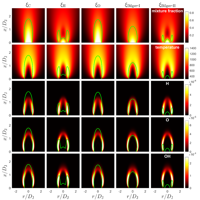
Figure 10: The contours of the mixture fraction (row 1), temperature (row 2), and the mole fractions of the radicals H (row 3), O (row 4), and OH (row 5) in a laminar round free jet H₂/CO₂-air non-premixed flame. Each column corresponds to a specific definition of the mixture fraction: $\xi_{\mathrm{C}}$ based on the element C only (column 1), $\xi_{\mathrm{H}}$ based on the element H only (column 2), $\xi_{\mathrm{O}}$ based on the element O only (column 3), $\xi_{\mathrm{Bilger\text{-}I}}$ in equation (14), and $\xi_{\mathrm{Bilger\text{-}II}}$ in equation (15). The lines are the iso line of the mixture fraction at the value of $\xi_{\mathrm{st}}=0.539$.

The simulation results are depicted in Figure 10 where the contours of the mixture fraction, temperature, and the mole fractions of the radicals H, O, and OH are shown. Five different mixture fraction definitions are compared: the single-element based mixture fractions ($\xi_{\mathrm{C}}$, $\xi_{\mathrm{H}}$, and $\xi_{\mathrm{O}}$), $\xi_{\mathrm{Bilger\text{-}I}}$, and $\xi_{\mathrm{Bilger\text{-}II}}$. The iso lines of the stoichiometric value $\xi_{\mathrm{st}}=0.539$ are also shown in the figure for the different mixture fraction definitions. A direct comparison of the different mixture fraction definitions (row 1 in Figure 10) shows some significant difference between some of the definitions. The two definitions $\xi_{\mathrm{H}}$ and $\xi_{\mathrm{Bilger\text{-}II}}$ shows distinctive profiles that are not seen in the other definitions: being non-monotomic and not continuous (or not smooth). Bilger-II yields two iso lines of $\xi=\xi_{\mathrm{st}}$. The stoichiometric condition occurs around the flame front that is indicated approximately by the peak locations of temperature and the radicals. The mismatch of the stoichiometric condition and the iso lines of $\xi=\xi_{\mathrm{st}}$ is evident for some of the definitions, particularly for $\xi_{\mathrm{H}}$ (column 2 in Figure 10) and $\xi_{\mathrm{Bilger\text{-}II}}$ (column 5). A good match is seen between the peak locations of the radicals (stoichiometric condition) and the iso lines of $\xi=\xi_{\mathrm{st}}$ when $\xi_{\mathrm{Bilger\text{-}I}}$ (column 4) is used. The iso lines of $\xi=\xi_{\mathrm{st}}$ obtained from $\xi_{\mathrm{C}}$ (column 1) and $\xi_{\mathrm{H}}$ (collumn 2) are close to the peak locations of the radicals, while the deviation is also visible.

Thus it is important for a properly defined mixture fraction to posses the stoichiometry preservation property so that the stoichiometric value $\xi_{\mathrm{st}}$ based on the definition can serve as a true representation of the actual stoichiometric condition.

Appendix B Flame front indicator in the mixture farction space

A flame front indicator $\xi_{\mathrm{F}}$ is used in this work that is defined as the average of the peak locations of the three common radicals OH, H, and O in the mixture fraction space, $\xi_{\mathrm{F}}=(\xi_{\mathrm{OH,max}}+\xi_{\mathrm{H,max}}+\xi_{\mathrm{OH,max}})/3$, where $\xi_{\alpha,\mathrm{max}}$ is defined as the peak location of the species $\alpha$ in the mixture fraction space, $Y_{\alpha}(\xi_{\alpha,\mathrm{max}})=\mathrm{max}(Y_{\alpha}(\xi))$. Here, we examine the efficacy of the indicator in opposed laminar jet flames. Figure 11 shows the profiles of the mass fractions $Y_{\mathrm{OH}}$, $Y_{\mathrm{H}}$, and $Y_{\mathrm{O}}$ in the mixture fraction space in the $\mathrm{CH_{4}/H_{2}}$ (mole ratio 1:1) opposed laminar jet flame (left column) and the H₂/CO₂ (mole ratio 36%:64%) opposed jet flame (right column) with $s=50\ s^{-1}$. The flame front indicated by the peak locations of the different radicals under different stretching conditions is shown in the figure too (bottom row). The ED model is used for the OPPDIF calculations in Figure 11. It is seen that the three radicals all peak around the stoichiometric condition with some slight deviation. The peak locations in the mixture fraction space vary when the strain rate $s$ changes. The average location of the three peak locations of the radicals, defined as $\xi_{\mathrm{F}}$, shows a slightly better match with the stoichiometric value $\xi_{\mathrm{st}}$ in both flames. We thus use the average of the three radical peak locations to indicate the flame front location $\xi_{\mathrm{F}}$ or $\xi_{\mathrm{F,ED}}$ in this work.

Figure 11: Calculation results for a CH₄/H₂-air opposed jet flame (left column) and a H₂/CO₂-air (right column) with $s=50\ s^{-1}$ and the equal molecular diffusion model. The top row shows the profiles of the radical mass fractions $Y_{\mathrm{OH}}$, $Y_{\mathrm{H}}$, and $Y_{\mathrm{O}}$ against the mixture fraction $\xi$, and the bottom row shows the variation of the flame front locations $\xi_{\mathrm{F,ED}}$ based on the peak locations of the radicals OH, H, and O and the average of the peak locations of the three radicals against the strain rate $s$. The dash-dotted lines indicate the value of $\xi_{\mathrm{st}}$.

Appendix C Linearity of the flame front location $\xi_{\mathrm{F}}$ against $b$

The observed linear variation of the flame front location $\xi_{\mathrm{F}}$ against $b$ in Figures 3 and 5 can be verified analytically, as demonstrated here. We rewrite the coupling function $\beta$ in the generalized mixture fraction in equation (10) as,

$$\beta=(z_{\mathrm{H}}-\mathcal{X}z_{\mathrm{C}})\cdot b+\left[(2+\mathcal{X}/2)z_{\mathrm{C}}-z_{\mathrm{O}}\right]=c_{3}\cdot b+c_{4},$$ (29)

where $c_{3}=(z_{\mathrm{H}}-\mathcal{X}z_{\mathrm{C}})$ and $c_{4}=\left[(2+\mathcal{X}/2)z_{\mathrm{C}}-z_{\mathrm{O}}\right]$. We first explore the properties of the two coefficients $c_{3}$ and $c_{4}$. In the $\{\mathrm{CH_{\mathcal{X}}}\}$-air or $\{\mathrm{CH_{\mathcal{X}}O_{\mathcal{Y}}}\}$-air combustion, the element mole ratio $z_{\mathrm{H}}:z_{\mathrm{C}}$ is $\mathcal{X}$ (equal diffusion) or slightly deviates from it due to differential molecular diffusion. In the limit of equal diffusion, $c_{3}=0$ and hence $\beta$ (and the generalized Bilger mixture fraction $\xi_{\mathrm{gen}}$) is not dependant on $b$. Under the effect of differential molecular diffusion, $c_{3}=(z_{\mathrm{H}}-\mathcal{X}z_{\mathrm{C}})$ is expected to be a small quantity at any location inside a flame, i.e., $c_{3}=O(\varepsilon)$, where $\varepsilon\ll 1$. For the coefficient $c_{4}$, it can be readily seen that $c_{4}$ is a small quantity near the flame front (stoichiometric condition), $c_{\mathrm{4,F}}=O(\varepsilon)$, where “F” denotes the flame front location. Under the limit of equal diffusion, $c_{4}$ is zero at the stoichiometric condition. Generally, $c_{4}$ is not small away from the flame front, i.e., $c_{4}=O(1)$ except near the flame front. With these properties of the coefficients $c_{3}$ and $c_{4}$, we next analyze the variation of the flame front $\xi_{\mathrm{F}}$ against $b$. Substituting equation (29) to equation (3) and evaluating the mixture fraction at the flame front, we obtain,

$$\xi_{\mathrm{F}}=\frac{(c_{\mathrm{3,F}}-c_{\mathrm{3,o}})\cdot b+(c_{\mathrm{4,F}}-c_{\mathrm{4,o}})}{(c_{\mathrm{3,f}}-c_{\mathrm{3,o}})\cdot b+(c_{\mathrm{4,f}}-c_{\mathrm{4,o}})},$$ (30)

where “f” and “o” denote the fuel and oxidizer boundaries, respectively. By using the properties of $c_{3}$ and $c_{4}$ above, we can readily find that $|(c_{\mathrm{3,f}}-c_{\mathrm{3,o}})\cdot b|\ll|c_{\mathrm{4,f}}-c_{\mathrm{4,o}}|$ in the denominator as long as $b=O(1)$ which is generally advised based on the discussion in this paper. Thus equation (29) can be simplified to,

$$\xi_{\mathrm{F}}\approx\frac{(c_{\mathrm{3,F}}-c_{\mathrm{3,o}})}{(c_{\mathrm{4,f}}-c_{\mathrm{4,o}})}\cdot b+\frac{(c_{\mathrm{4,F}}-c_{\mathrm{4,o}})}{(c_{\mathrm{4,f}}-c_{\mathrm{4,o}})},$$ (31)

Therefore, the linearity of $\xi_{\mathrm{F}}$ with respect to the free parameter $b$ is analytically verified, which supports the numerical observations in Figures 3 and 5.

References

- [1] R. Bilger, Turbulent diffusion flames, Annu Rev Fluid Mech 21 (1989) 101–135.
- [2] N. Peters, Laminar diffusion flamelet models in non-premixed turbulent combustion, Prog Energ Combust Sci 10 (1984) 319–339.
- [3] R. W. Bilger, Conditional moment closure for turbulent reacting flow, Phys Fluids 5 (1993) 436–444.
- [4] S. P. Burke, T. E. Schumann, Diffusion flames, Ind Eng Chem 20 (1928) 998–1004.
- [5] R. W. Bilger, The structure of diffusion flames 13 (1976) 155–170.
- [6] H. Pitsch, N. Peters, A consistent flamelet formulation for non-premixed combustion considering differential diffusion effects, Combust Flame 114 (1998) 26–40.
- [7] R. Bilger, The structure of turbulent nonpremixed flames, Proc Combust Inst 22 (1988) 475–488.
- [8] R. Bilger, S. Starner, R. Kee, On reduced mechanisms for methane-air combustion in nonpremixed flames, Combust Flame 80 (1990) 135–149.
- [9] A. Masri, R. Dibble, R. Barlow, Chemical kinetic effects in nonpremixed flames of H2/CO2 fuel, Combust Flame 91 (1992) 285–309.
- [10] J. C. Hewson, A. R. Kerstein, Local extinction and reignition in nonpremixed turbulent CO/H2/N2 jet flames 174 (2002) 35–66.
- [11] A. R. Masri, R. W. Dibble, R. S. Barlow, The structure of turbulent nonpremixed flames of methanol over a range of mixing rates, Combust Flame 89 (1992) 167–185.
- [12] A. R. Masri, R. W. Dibble, R. S. Barlow, Raman-rayleigh measurements in bluff-body stabilised flames of hydrocargon fuels, Symp (Int) on Combust 24 (1992) 317–324.
- [13] M. Roomina, R. Bilger, Conditional moment closure modelling of turbulent methanol jet flames, Combust Theor Model 3 (1999) 689–708.
- [14] N. Peters, Turbulent Combustion, Cambridge University Press, 2000.
- [15] S. Gierth, F. Hunger, S. Popp, H. Wu, M. Ihme, C. Hasse, Assessment of differential diffusion effects in flamelet modeling of oxy-fuel flames, Combust Flame 197 (2018) 134–144.
- [16] S. Stårner, R. Bilger, J. Frank, D. Marran, M. Long, Mixture fraction imaging in a lifted methane jet flame, Combust Flame 107 (1996) 307–313.
- [17] R. L. Gordon, C. Heeger, A. Dreizler, High-speed mixture fraction imaging, Appl Phys B 96 (2009) 745–748.
- [18] C. Wall, B. J. Boersma, P. Moin, An evaluation of the assumed beta probability density function subgrid-scale model for large eddy simulation of nonpremixed, turbulent combustion with heat release, Phys Fluids 12 (2000) 2522–2529.
- [19] H. Wang, P. Zhang, J. Tao, Examination of probability distribution of mixture fraction in LES/FDF modelling of a turbulent partially premixed jet flame, Combust Theor Model 26 (2022) 320–337.
- [20] H. Wang, Consistent flamelet modeling of differential molecular diffusion for turbulent non-premixed flames, Phys Fluids 28 (2016) 035102.
- [21] R. Barlow, J. Frank, Effects of turbulence on species mass fractions in methane/air jet flames, Proc Combust Inst 27 (1998) 1087–1095.
- [22] F. A. Williams, Combustion Theory, 2nd Edition, CRC Press, 1985.
- [23] A. E. Lutz, R. J. Kee, J. F. Grcar, F. M. Rupley, OPPDIF: A FORTRAN program for computing opposed-flow diffusion flames, Tech. rep., Sandia National Laboratories, SAND96-8243, Livermore, CA (1997).
-
[24]
H. Wang, X. You, A. V. Joshi, S. G. Davis, A. Laskin, F. Egolfopoulos, C. K.
Law, High-temperature
combustion reaction model of H2/CO/C1-C4 compounds (2007-05).
URL http://ignis.usc.edu/USC_Mech_II.htm - [25] R. Barlow, G. Fiechtner, C. Carter, J.-Y. Chen, Experiments on the scalar structure of turbulent CO/H2/N2 jet flames, Combust Flame 120 (2000) 549–569.
- [26] R. Barlow, J. Frank, Effects of turbulence on species mass fractions in methane/air jet flames, Proc Combust Inst 27 (1998) 1087–1095.
- [27] F. Fuest, R. S. Barlow, J.-Y. Chen, A. Dreizler, Raman/Rayleigh scattering and CO-LIF measurements in laminar and turbulent jet flames of dimethyl ether, Combust Flame 159 (2012) 2533–2562, special Issue on Turbulent Combustion.
- [28] L. Smith, R. Dibble, L. Talbot, R. Barlow, C. Carter, Laser Raman scattering measurements of differential molecular diffusion in turbulent nonpremixed jet flames of H2/CO2 fuel, Combust Flame 100 (1995) 153–160.
-
[29]
The San
Diego mechanism (2016-12-14).
URL https://web.eng.ucsd.edu/mae/groups/combustion/mechanism.html - [30] H. Tang, C. Yang, G. Wang, Y. Krishna, T. F. Guiberti, W. L. Roberts, G. Magnotti, Scalar structure in turbulent non-premixed NH3/H2/N2 jet flames at elevated pressure using raman spectroscopy, Combust Flame 244 (2022) 112292.
- [31] J. Otomo, M. Koshi, T. Mitsumori, H. Iwasaki, K. Yamada, Chemical kinetic modeling of ammonia oxidation with improved reaction mechanism for ammonia/air and ammonia/hydrogen/air combustion, Int J Hydrog Energy 43 (2018) 3004–3014.
- [32] Y. Song, H. Hashemi, J. M. Christensen, C. Zou, B. S. Haynes, P. Marshall, P. Glarborg, An exploratory flow reactor study of H2S oxidation at 30–100 Bar, Int J Chem Kinet 49 (2017) 37–52.
-
[33]
ANSYS FLUENT User’s
Guide (Version: 2020R1) (2021).
URL https://www.ansys.com/products/fluids/ansys-fluent