Abstract

Entertaining the possibility of time travel will invariably challenge dearly held concepts of fundamental physics. It becomes relatively easy to construct multiple logical contradictions using differing starting points from various well-established fields of physics. Sometimes, the interpretation is that only a full theory of quantum gravity will be able to settle these logical contradictions. Even then, it remains unclear if the multitude of problems could be overcome. Yet as definitive as this seems to the notion of time travel in physics, such a recourse to quantum gravity comes with its own, long-standing challenge to most of these counter-arguments to time travel: These arguments rely on time, while quantum gravity is (in)famously stuck with and dealing with the problem of time. One attempt to answer this problem within the canonical framework resulted in the Page–Wootters formalism, and its recent gauge-theoretic re-interpretation—as an emergent notion of time. Herein, we will begin a programme to study toy models implementing the Hamiltonian constraint in quantum theory, with an aim towards understanding what an emergent notion of time can tell us about the (im)possibility of time travel.

1 1 0 https://doi.org/ Emergent Time and Time Travel in Quantum Physics Emergent Time and Time Travel in Quantum Physics Ana Alonso-Serrano ^1,2,†, Sebastian Schuster^3,†* and Matt Visser ^4,† Ana Alonso-Serrano, Sebastian Schuster and Matt Visser Alonso-Serrano, A.; Schuster, S.; Visser, M. Correspondence: sebastian.schuster@utf.mff.cuni.cz These authors contributed equally to this work.

1 Introduction

As fascinating as the notion of time travel is, its long list of problematic issues—ranging from the classical Roman (1993); Krasnikov (2002), (Visser, 1997, p.212ff) to the quantum theoretical Hawking (1992); Klinkhammer (1992); Visser (1993); Emparan and Tomašević (2022)—presents a very solid case against it, and its absence is effectively a feature of the universe accessible to human experience. Yet if one wants to look closely at these arguments, cracks and loopholes start to appear—many of which shall be mentioned in the following. To an extent, it almost seems as if the best evidence against any notion of time travel is that of our daily experienced notion of time and causality, our intuition. Still, the known universe is bigger than our day-to-day experience, and particularly the field of high energy physics is ripe with examples experimentally, observationally, or theoretically open to inquiry—in which various concepts or preconceived notions of human-scale physics have to be let go. In no field of theoretical physics is this more apparent than in the quest for quantum gravity. The field of contenders is large, and still growing: String theory, loop quantum gravity, quantum geometrodynamics, asymptotic safety, causal dynamical triangulation, causal set theory, Hořava–Lifshitz gravity, …Each comes with its own set of new notions beyond what can be experienced directly by human senses. Yet, these proposals still have to address, in one way or another, an issue plaguing quantum gravity from its beginning: Time. This problem of time, and its eventual resolution, then naturally will also impact what these theories have to say about (or against) time travel.

Classically, the ‘problem of time’ in canonical gravity is settled by a careful, gauge-theoretic analysis Pons et al. (2010) that distinguishes the different rôles played by the Hamiltonian, either in the constraint/gauge fixing or in the definition of observables, respectively. In quantum gravity, however, the problem of time remains (at the very least) a topic of active discussion and research Anderson (2017); Kiefer and Peter (2022). The reason for this goes back even before a theory of quantum gravity was the focus: While there are ways to give position and momentum a meaning in terms of operators on (rigged) Hilbert spaces in quantum mechanics, this cannot be carried over to time and energy. This was concerning to researchers in quantum mechanics early on, as the time-energy uncertainty relations proved to be both reliable and instructive, while not fitting into the standard paradigm of the Robertson–Schrödinger uncertainty relations for (generic) Hermitian operators. Only the proof of Mandelstam and Tamm in 1945 improved this uncertainty relation’s foundation, while begging the question of why a different approach was needed Mandelstam and Tamm (1945). Essentially, a series of impossibility results for time operators canonically conjugate to a Hamiltonian was presented: Schrödinger used an approach based on normalizability Schrödinger (1931), similar to the argument for why plane waves require a rigged Hilbert space. Pauli, in a footnote, used a simpler argument juxtaposing discrete spectra and the continuous translation in energy such a time operator would induce Pauli (1990, 1980). Finally (and in reply to what will be discussed shortly), Unruh and Wald gave a general argument for semi-bounded Hamiltonians linked to unitarity Unruh and Wald (1989). Two at first glance quite distinct approaches were developed in reply to these no-go results.

One approach was similar in spirit to the answer to early counterarguments to plane waves, e.g., eigenstates of definite position and momentum. While with position and momentum one relaxes the idea of being restricted to Hilbert space and instead works in a rigged Hilbert space Böhm (1993); de la Madrid et al. (2002); Thiemann (2008), here, when faced with the above-cited no-go results concerning time operators, one relaxes the idea of Hermiticity. Instead, one introduces the notion of a positive, operator-valued measure (POVM). It can represent not just perfect measurements yielding a definite eigenstate, but also imprecise measurements Busch et al. (2016). Besides allowing one to address the measurement problem in quantum field theory Fewster and Verch (2020), phase observables Busch et al. (1995), or the already mentioned, imprecise measurement processes Auletta et al. (2009); Busch et al. (2016)—and more important for the present context—this allows a notion of time measurement Busch et al. (1994). Since the no-go theorems relate to Hermitian operators, the more general POVMs are not ruled out as time observables. As we will see, the context of time travel allows one to avoid these no-go results by other means, too. Still, the bigger picture of gauge theory provides the most pertinent background for extensions of the model to be described in this paper.

Another approach that developed independently from POVMs was to carefully distinguish between a clock and time. Paraphrasing Einstein Einstein (1905), time is meaningful only after specifying the clock measuring it. Early on, in developing canonical quantum gravity, DeWitt DeWitt (1967) pointed out how different subsystem’s operators in a given Hamiltonian constraint could serve this purpose of an effective clock. Page and Wootters then took this idea and made it more general and workable, by phrasing time evolution in terms of conditional probabilities linking different subsystems Page and Wootters (1983); Wootters (1984). This Page–Wootters (PW) formalism was soon challenged on various grounds by Unruh, Wald Unruh and Wald (1989) and Kuchař Kuchař (2011), leading to this approach lying dormant for some time.

Recent developments then made the latter approach re-emerge Giovannetti et al. (2015); Marletto and Vedral (2017); Gemsheim and Rost (2023), and both approaches converge Smith and Ahmadi (2019); Höhn et al. (2021a). This also allowed one to address and re-contextualize the earlier criticisms of the PW formalism Höhn et al. (2021a, b). In essence, the clocks chosen within the PW formalism become part of a gauge-theoretic picture of clocks; the ‘physical Hilbert space’ being a ‘clock-neutral’ picture, and different clocks representing different ‘gauge conditions’ Höhn et al. (2021a). These results form part of a larger research programme that aims to ground the rulers and clocks at least implicitly employed in external symmetries with an operational underpinning Krumm et al. (2021); Goeller et al. (2022); Adlam (2022); Höhn et al. (2023); Hausmann et al. (2023); Höhn et al. (2023). For our purposes below, the key takeaway is that the PW formalism still works, if its defects and the criticisms of it are understood as related to issues already familiar from electromagnetism: One has to choose whether a calculation should be gauge-fixed or gauge-independent. Depending on the question at hand, one or the other will be better suited to calculations or understanding. Our model below will be too simple to fully showcase these developments, but given the criticisms the PW formalism faced, it is important to keep the resolution in mind.

Within this special issue’s scope, many other pertinent links of time and time travel to quantum physics could be made. A selected, non-exhaustive list would include: Deutsch CTCs and (non/retro-)causal quantum processes Deutsch (1991); Bishop et al. (2021); Baumann et al. (2022); Vilasini (2021); Adlam (2022), simulation of time travel in analogues Barceló et al. (2022); Sabín (2022), semi-classical/quantum stability Hawking (1992); Klinkhammer (1992); Visser (1993); Emparan and Tomašević (2022), et cetera. For the purposes of this article, however, we would like to highlight only two further research avenues. One is that of different notions of time. Yet another, non-exhaustive list would include at least cosmological time, psychological time, parameter time, thermodynamic time, dynamical versus kinematical time, …While this distinction is studied mostly in the context of ‘the arrow of time’ Zeh (2007), it is worth pointing out that many counterarguments to time travel have to rely at least on some conflation of these concepts. To give just one example, if thermodynamic arguments are brought forth, one needs to establish a more or less direct relation between the thermodynamic notion implied by the second law and the notion of time invoked in time travel. (This itself does not have to be the same notion as that of general relativity (GR), where time travel can be identified with closed, time-like curves (CTCs) or related concepts Minguzzi and Sánchez (2006). In theories other than GR, a different notion of time might be relevant to describe time travel!)

The other important point to make is that despite all the counterarguments, time travel is just one notion of many with questionable ‘physicality.’ Even within the context of GR, other notions of physicality vie for validity with the absence of time travel, for example, various kinds of completeness (geodesic, hole free, …) or the validity of various kinds of energy conditions. These notions, however, are not all compatible with each other Barcelo and Visser (2002); Earman et al. (2009); Manchak (2009, 2018, 2021); Santiago et al. (2022). One might find oneself in the uncomfortable situation that a dearly held and important property (stability, completeness, fulfilled energy conditions, …) will require time travel to be permitted; and this just within GR. Other theories are unlikely to be free from such problems, especially as many of the comforting no-go theorems are specifically proven within the context of GR. It it therefore not surprising that in the context of classical field theories of gravity alone, there exist many different ways to realize time travel. This includes wormholes Visser (1997); González-Díaz and Alonso-Serrano (2011), warp drives Everett (1996), cosmologies Gödel (1949); Hawking and Ellis (1974); Griffiths and Podolský (2012); Gray et al. (2017), maximally extended space-times (such as Kerr near the central ring singularity) Wald (1984), and various more mathematical construction techniques Penrose (1972); Krasnikov (1998); Manchak (2011). The latter can also be employed to distinguish between, for example, time travel (CTCs) and time machines (whatever structure creates or causes CTCs) Earman et al. (2009); Manchak (2009, 2011).

This finally brings us to the goal of this paper: We want to study what can be said about the viability of time travel if time itself is only an emergent concept, as in the PW formalism. Concretely, we will be studying an example of two non-interacting harmonic oscillators subjected to a Wheeler–DeWitt (WDW) equation, i.e., it will represent in some sense a minisuperspace model of time travel. This toy model is by no means meant to exhibit an exhaustive description of whether and how time travel can arise in the PW formalism. We will see that the results in our toy model point to an extraordinarily bland version of Novikov’s self-consistency conjecture Novikov (1992); Sklar (1990); Friedman et al. (1990).

1.1 Outline

Following the preceding introduction to and overview of the related research question in section 1, we will provide an introduction into the methods employed: In section 2, we briefly summarize the PW formalism. In section 3 we demonstrate POVM’s utility for implementing time observables in the context of a single harmonic oscillator. The main part of the paper is employing these concepts then, in section 4, to two harmonic oscillators subjected to a WDW-like Hamiltonian constraint equation. We close by discussing our results and pointing out future directions and open questions in section 5. Finally, the appendices collect additional details and context: Appendix A reviews the mathematical definition of a POVM, appendix B collects results concerning periodic time in the quantum harmonic oscillator that supplement the discussion of section 3.1, while appendix C gives additional details concerning the construction of the paper’s figures.

We will use natural units in which $G=\hbar=c=1$.

2 The Page–Wootters Formalism

Let us consider a quantum system (‘the universe’) that separates into two subsystems, a ‘clock’ system and a ‘residual’ system. The PW formalism is our first, and most important ingredient for studying time travel without time (or rather: time travel with only an emergent notion of time). It is a proposal to give an operational meaning to measuring the time evolution of the residual subsystem in the larger quantum system (the ‘universe’) with respect to the other, (mostly) decoupled ‘clock’ subsystem. Partly, this separation into ‘clock’ and ‘residual’ (in the literature often ‘rest’) systems is motivated by the problem of time encountered in quantum gravity. In terms of the total Hilbert space $\mathcal{H}$, the clock Hilbert space $\mathcal{H}_{\textsc{c}}$, and $\mathcal{H}_{\textsc{r}}$, the residual Hilbert space, this means:

$$\mathcal{H}=\mathcal{H}_{\textsc{c}}\otimes\mathcal{H}_{\textsc{r}}.$$ (1)

Subsequent developments and refinements sometimes further separated what we call $\mathcal{H}_{\textsc{r}}$ into evolving and ancillary/memory/supplementary/…systems, but for our purposes, we will not follow this line of thinking—at least in this current paper. In future work, it could be interesting to see whether such an approach could provide a notion of time travel that—contrary to GR’s CTCs—only allows for a finite number of temporal round trips. Each of these Hilbert spaces is equipped with a Hamiltonian acting on these separate Hilbert spaces, such that

$$\hat{H}\ket{\Psi}=\left(\hat{H}_{\textsc{c}}\otimes\mathds{1}_{\textsc{r}}+\mathds{1}_{\textsc{c}}\otimes\hat{H}_{\textsc{r}}\right)\ket{\Psi}=E\ket{\Psi},$$ (2)

where $\ket{\Psi}$ is a state in the total Hilbert space $\mathcal{H}$. In line with Schrödinger’s 1931 footnote, this state $\ket{\Psi}$ is required to be in a definite, fixed eigenstate of $\hat{H}$ with total energy $E$. More generally, the PW formalism remains viable even for density matrices $\hat{\rho}$, with the above case regained by setting $\hat{\rho}=\ket{\Psi}\bra{\Psi}$.

Examples of such systems usually are constructed by symmetry-reducing the WDW equation of quantum gravity, the quantized Hamiltonian constraint of GR:

$$\hat{H}\ket{\Psi}=0.$$ (3)

In this expression, we gloss over many technicalities (such as operator ordering, domain issues, topological concerns, configuration space considerations, …) DeWitt (1967); Thiemann (2008); Kiefer (2012), as our focus lies less on quantum gravity and more on the emergent notion of time that the PW formalism provides. Still, we will occasionally take inspiration from quantum gravity. In particular, one can consider our final model to be a crude example of a minisuperspace model that has not been found through symmetry reduction. Already here, we therefore want to point out that many questions the minisuperspace models of quantum black holes or quantum cosmology try to answer, will not and cannot appear in our context. Most notably will be an absence of gravitational singularities, whose avoidance has been a mainstay of quantum gravity.

The key step for formulating the PW formalism now lies in describing the evolution of the system encoded through a tuple $(\mathcal{H}_{\textsc{r}},\hat{H}_{\textsc{r}})$ in terms of the evolution of $(\mathcal{H}_{\textsc{c}},\hat{H}_{\textsc{c}})$. For this, one picks some initial state $\ket{\psi(0_{\ast})}_{\textsc{c}}\in\mathcal{H}_{\textsc{c}}$, which is then evolved using the clock Hamiltonian according to

$$\ket{\psi(\theta_{\ast})}_{\textsc{c}}\mathrel{\mathop{:}}=e^{-i\hat{H}_{\textsc{c}}\theta_{\ast}}\ket{\psi(0_{\ast})}_{\textsc{c}}.$$ (4)

This corresponds to the familiar idea of unitary time evolution of states in the Schrödinger picture through a Hamiltonian, but—at this level of the discussion, anyway—is a definition. The Schrödinger or Heisenberg equations of motion would then be a result of this approach Page and Wootters (1983); Smith and Ahmadi (2019).

The evolution of the subsystem $\hat{H}_{\textsc{r}}$ is then evaluated in terms of relative probabilities with respect to these clock states. To do this, let us first define the projector

$$\hat{P}_{\theta_{\ast}}\mathrel{\mathop{:}}=\left(\ket{\psi(\theta_{\ast})}_{\textsc{c}}\ {\vphantom{\bra{\psi({{\theta}_{\ast}})}}}_{\textsc{c}}\!\bra{\psi({{\theta}_{\ast}})}\right)\otimes\mathds{1}_{\textsc{r}}$$ (5)

of a given state onto particular ‘clock time states’ $\ket{\psi(\theta_{\ast})}_{\textsc{c}}$ in $\mathcal{H}_{\textsc{c}}$, leaving states in $\mathcal{H}_{\textsc{r}}$ unchanged. Then the evolution in $\mathcal{H}_{\textsc{r}}$ by $\hat{H}_{\textsc{r}}$ with respect to clock states is given by the expression

$$E(\hat{H}_{\textsc{r}}|\theta_{\ast})=\frac{\operatorname{tr}\left(\hat{H}_{\textsc{r}}\hat{P}_{\theta_{\ast}}\hat{\rho}\right)}{\operatorname{tr}\left(\hat{P}_{\theta_{\ast}}\hat{\rho}\right)}.$$ (6)

This gives the conditional expectation value of the residual Hamiltonian $\hat{H}_{\textsc{r}}$ when the clock (state) ‘reads’ $\theta_{\ast}$. The technical requirements behind this interpretation are stationarity,

$$[\hat{H},\hat{\rho}]=0,$$ (7)

and commutativity of $\hat{H}_{\textsc{r}}$ and $\hat{H}_{\textsc{c}}$, which we enforced by the block structure of $\hat{H}$ encoded in equation (2). These assumptions are quite strong, especially once one wants to include an interaction Hamiltonian coupling $\mathcal{H}_{\textsc{c}}$ and $\mathcal{H}_{\textsc{r}}$ on the right hand side of equation (2). Given the recent clarification on this issue provided by Giovannetti et al. (2015); Marletto and Vedral (2017); Smith and Ahmadi (2019); Höhn et al. (2021a), we want to return to such generalizations at a later point, but stick to these more restrictive assumptions in the present context.

Some general comments are appropriate at this point: First, fixing the initial, total state $\ket{\Psi}$ can, in general, greatly change the time evolution as described by equation (6). Second, to reiterate: This is not the most sophisticated or modern implementation of the PW formalism, see the previous paragraph. Third, without further specifying a particular system comprised of the various Hamiltonians present in equation (2), we cannot even begin our investigation. This holds true for the sort of time evolution people expect—one without time travel—just as well as for the more unexpected time evolution—showcasing a notion of time travel. The next step will be to lay the groundwork for our toy model, specifying the state and the evolution.

2.1 Time Travel in the Page–Wootters Formalism

In order to prepare this next step, let us first connect the PW formalism to some of the notions mentioned in the introduction. In particular, we would like to be able to talk about time travel in this setting. The simplest way to achieve this is to demand that the domain from which our time parameter $\theta$ is taken to be $S^{1}$, i.e., periodic. By itself, this will not guarantee a useful notion of time travel. A simple way to see this is by looking at everyday clocks: They are all periodic. Only a calendar, also keeping track of years, would be a truly non-periodic clock. One does not travel back in time when one wakes up at the same time each morning, just because the alarm clock is periodic.

Instead, we will try to find a way to implement the simplest possible version of time travel. This is (Novikov) self-consistency. When the clock returns to a state, so will the remainder system return to the same state it had when the clock last was in this state. This situation can (at least in some systems and models) also yield existence results, though usually at the expense of uniqueness Friedman et al. (1990); Echeverria et al. (1991); Fewster et al. (1996); Bachelot (2002); Dolanský and Krtouš (2010). So far, however, the PW formalism as presented here does not allow for this. The evolution of the clock as prescribed by equation (4) is ignorant of the domain from which to draw $\theta_{\ast}$.

In order to alleviate this problem, we will borrow concepts from the POVM approach to time operators already mentioned in the introduction, and to be discussed in more detail in the next section. In order to incorporate this in the PW formalism, we note that the key ingredient for comparing the evolution of the clock with that of the remainder system is encoded in the definition of the projector onto clock states, equation (5). The goal, thus, will be to not only influence the clock evolution through a convenient choice of the global state $\ket{\Psi}$. Rather, we also will have to make a judicious choice of the clock states themselves, and how to identify them in a meaningful way.

3 POVMs, the Harmonic Oscillator, and Time

The second ingredient of our investigation is a particularly simple example of time operators and POVMs: The harmonic oscillator Susskind and Glogower (1964); Garrison and Wong (1970); Galindo (1984); Busch et al. (1994, 1995). As an ubiquitous model system in all fields of classical and quantum physics, it is likely to be an instructive ingredient even in our systems following a Hamiltonian constraint similar to the WDW equation (3). Our discussion will follow the presentation of the two just-mentioned articles, adapted to the notation chosen for our application. Concretely, it is possible in the POVM framework to introduce time with a periodic domain through a phase POVM. Similar to time operators, also an operator representing a phase variable has been difficult to construct in a mathematically rigorous manner. Here, the problems are tied to issues of boundary conditions, hermiticity, and the domain of operators not given in standard notation. As with time operators, the more general setting of POVMs provides a way around this. Since a time operator ideally would be canonically conjugate to the Hamiltonian (as suggested by the energy-time uncertainty relation), and a phase operator ideally would be canonically conjugate to the number operator, the connection to periodic time is easily made.

In our toy model of harmonic oscillators (further specified below in section 4), we will identify phase and time. This is also provides the easiest way to rigorously define time travel, making use of Novikov’s self-consistency conjecture: A system comprised of clock and dynamical system with respect to clock time undergoes time travel, if the dynamical system state is the same after each full clock period. This definition could, in principle, be relaxed. For example, this could happen only a finite number of times. An emergent notion of time furthermore allows one to make such a statement merely approximate. This will allow us to study rigorously notions of time travel that not fully fall into this framework of self-consistency; for example, only parts of the system could undergo time travel. We hope that such models including the clock itself can shed light on when a system is ‘merely periodic in time’ versus when it actually undergoes time travel. In our final section 5, we will further expound on this. Importantly, a requirement of self-consistency will preempt any of the traditional paradoxa constructed out of it.

3.1 Time and Phase Operators for the Harmonic Oscillator

Leaving the mathematical formalities (mostly) aside, we will now introduce the specific POVM used in our simple model of time travel. Formal, supplementary details regarding the definition of POVMs can be found in appendix A. For the purposes of this section, we will drop all label indices, and only look at the simple, standard harmonic oscillator with Hamiltonian

$$\hat{H}=\frac{1}{2}\hat{a}^{\dagger}\hat{a}+\frac{1}{2}.$$ (8)

We want to construct a time operator for this. In order to do so, we look at the polar decomposition of the ladder operator $\hat{a}$, (Reed and Simon, 1980, Thm. VIII.32):

$$\hat{a}=\hat{W}\widehat{\left\lvert a\right\rvert}.$$ (9)

Here, $\widehat{\left\lvert a\right\rvert}$ is easy to define as

$$\widehat{\left\lvert a\right\rvert}\mathrel{\mathop{:}}=\hat{n}^{1/2}=\sqrt{\hat{a}^{\dagger}\hat{a}}.$$ (10)

The ‘operator’ $\hat{W}$, however, is less simple than its occurrence in a ‘polar decomposition’ might suggest: It will not be unitary. More concretely Busch et al. (1995):

$$\hat{W}\hat{W}^{\dagger}=\mathds{1},$$ (11)

but

$$\hat{W}^{\dagger}\hat{W}=\mathds{1}-\ket{0}\negthickspace\bra{0}\neq\mathds{1}.$$ (12)

The phase or time states to be used are now constructed as eigenstates $\ket{\theta}$ of $\hat{W}$.

$$\hat{W}\ket{\theta}=e^{i\theta}\ket{\theta}.$$ (13)

While these eigenstates do exist, given the properties of $\hat{W}$, they are now only an overcomplete set of eigenstates. So different eigenstates $\ket{\theta}$ and $\ket{\theta^{\prime}}$ will not be orthogonal, and expressing a general state $\ket{\psi}$ in terms of these eigenstates will not be unique anymore. Each of these states $\ket{\theta}$ can be written as

$$\ket{\theta}=\sum_{n\geq 0}e^{in\theta}\ket{n}.$$ (14)

Now is the time to define a concrete POVM. In this instance, let us define for all Borel sets $X$ of $[0,2\pi)$

$$B_{0}(X) \mathrel{\mathop{:}}=\frac{1}{2\pi}\int_{X}\ket{\theta}\negthickspace\bra{\theta}\operatorname{d}\!\theta,$$ (15)

$$=\sum_{n,m\geq 0}\frac{1}{2\pi}\int_{X}e^{i(n-m)\theta}\ket{n}\negthickspace\bra{m}\operatorname{d}\!\theta.$$ (16)

The index $0$ is a first indication of what is to come: Different points on the unit circle $S^{1}$ can be chosen as starting points. In the above definition, one starts on the positive real axis, i.e., we choose our angle $\theta$ from $[0,2\pi)$, as opposed to say from $[\theta_{\ast},\theta_{\ast}+2\pi)$ for some $\theta_{\ast}\in[0,2\pi)$.

Using

$$\frac{1}{2\pi}\int_{o}^{2\pi}e^{i(n-m)\theta}\operatorname{d}\!\theta=\delta_{nm}$$ (17)

and

$$\sum_{n=0}^{\infty}\ket{n}\negthickspace\bra{n}=\mathds{1}$$ (18)

one can show that

$$B_{0}([0,2\pi))=\mathds{1},$$ (19)

which means that $B_{0}$ is a normalized POVM. So $B_{0}$ represents an observable in the sense of POVMs. Note that in the context of the definition of a POVM, in the present example we have that $\Omega=S^{1}$.

From the POVM side of things, this gives all ingredients needed for the calculations to follow. However, for a more comprehensive understanding of the physics of time involved in the harmonic oscillator, it is worthwhile to point out additional considerations concerning such periodic time variables. We have collected these observations in appendix B.

4 Time Travel in Two Harmonic Oscillators Subject to a Hamiltonian Constraint

The goals for the present article are modest. We want to study as simple a model as possible that is subject to a constraint reminiscent of the WDW equation (3). As we also want to capture time travel as defined above, we need for this two ingredients: A periodic clock system $(\mathcal{H}_{\textsc{c}},\hat{H}_{\textsc{c}})$ and a system $(\mathcal{H}_{\textsc{r}},\hat{H}_{\textsc{r}})$ that evolves in the sense of the PW formalism (at least) as periodic as the clock itself. Then it would be an instance of a quantum system fulfilling the Novikov self-consistency conjecture. Based on the discussion of harmonic oscillators above, the simplest such system would be to use a single harmonic oscillator for each $\hat{H}_{\textsc{r}}$ and $\hat{H}_{\textsc{c}}$, respectively. To allow for some more generality, we will not demand their respective frequencies $\omega_{\textsc{r}}$ and $\omega_{\textsc{c}}$ to be the same, a priori. Then, our model will have the following Hamiltonian in the full Hilbert space $\mathcal{H}$:

$$\hat{H}\ket{\Psi}=\left(\vphantom{\omega_{\textsc{c}}\,\hat{n}+\omega_{\textsc{c}}\frac{1}{2}\mathds{1}_{\textsc{c}}}\smash{\underbrace{\omega_{\textsc{c}}\,\hat{n}_{\textsc{c}}+\frac{\omega_{\textsc{c}}}{2}\,\mathds{1}_{\textsc{c}}}_{\hat{H}_{\textsc{c}}}\underbrace{-\omega_{\textsc{r}}\,\hat{n}_{\textsc{r}}-\frac{\omega_{\textsc{r}}}{2}\,\mathds{1}_{\textsc{r}}}_{-\hat{H}_{\textsc{r}}}}\right)\ket{\Psi}=0.\vphantom{\underbrace{\omega_{\textsc{c}}\hat{n}+\omega_{\textsc{c}}\frac{1}{2}\mathds{1}_{\textsc{c}}}_{\hat{H}_{\textsc{c}}}}$$ (20)

This means that the system Hamiltonian $\hat{H}_{\textsc{r}}$ and the clock Hamiltonian $\hat{H}_{\textsc{c}}$ are part of a WDW-like equation. Naturally, this implies that it falls into the framework of the PW formalism for a stationary Hamilton equation $\hat{H}\ket{\Psi}=E\ket{\Psi}$ with energy $E=0$.

The previous two sections gave us the two most important ingredients in place: First, the way to measure time evolution with respect to a clock system using the PW formalisms conditional probability (6). Second, the required clock states given by equation (13) with respect to which we will measure evolution, and its representation in terms of the harmonic oscillator eigenstates, equation (14). Now, we can make use of it by implementing the Hamiltonian constraint (20) into this model. What remains to be done, though, is to specify more explicitly the type of total state $\ket{\Psi}\in\mathcal{H}$ the ‘universe’ (as described by $\hat{H}$) is in.

4.1 Important Note on the Difference to Quantum Cosmology

Having introduced the model, it is easy to recognize it as a variant of a model already used in the context of quantum cosmology Kiefer (1989, 1990); Page (1991); Brunetti et al. (2010). There is, however, an important distinction both mathematically and interpretationally. One of the goals of quantum cosmology is to use symmetry reduction to arrive at minisuperspace models testing aspects of quantum gravity. In the context of (quantum) cosmology, this is in particular often the status of Hawking-type singularity theorems in quantum gravity: Can a cosmological singularity be avoided or not Hawking and Ellis (1965); DeWitt (1967); O’Neill (1983); Kiefer (2012)? In many, if not most situations this leads to the demand that the configuration space $\mathds{R}^{2}$ of the two harmonic oscillators is limited to the half-plane $\mathds{H}^{2}$, as one of the variables corresponds to the non-negative scale factor $a$. The scale factor at $a=0$ corresponds to a gravitational singularity. Restricting one harmonic oscillator to only a half-plane for its configuration space variable, however, inevitably leads to the inability to use the very convenient, powerful, and simple algebraic methods in terms of ladder operators used so far in the present paper.

Our present goals, however, are different. We want to study time travel in a quantum-theoretic framework, but in a manner that is as theory-agnostic as possible. Hence, we will simply not assume that equation (20) necessarily has its origins in a Hamiltonian formulation of general relativity or similar gravitational theories. This means that equation (20) with the domain used is an explicit input. It very well could be derived from a specific gravitational model in a specific gravitational theory through symmetry-reduction. Should this not be possible, it still may serve as a toy model. Especially, as the process of symmetry-reduction (to arrive at minisuperspace models) itself may be a fraught undertaking. Our assumption will be that such an equation with the full configuration space $\mathds{R}^{2}$ is available, and, likewise, so are our corresponding trusty ladder operators. This also bypasses issues such as the precise nature of the inner product on the quantum gravitational wavefunctions, as already discussed in (DeWitt, 1967, §9). Two extremal options for inner products (with many in between) are a quantum harmonic oscillator on the one side and a wave equation on the other. We assume the inner product structure as the one familiar from and resulting in standard quantum mechanics. Naturally, this leads to many directions into which to extend our present model, and we will come back to these in our concluding section 5.

In conclusion and in conscious distinction to quantum cosmology, our toy model (20) for time travel will be treated using a ladder operator approach of quantum mechanics. This allows us to use the methods introduced in the previous two section, and hopefully also provides easy extensions in diverse directions.

4.2 A Boring Model of Time Travel

Looking for a square-integrable solution to equation (20) introduces a new, additional condition on this equation. Only if

$$\frac{\omega_{\textsc{r}}}{\omega_{\textsc{c}}}=\frac{2n_{\textsc{c}}+1}{2n_{\textsc{r}}+1},\qquad\text{where\leavevmode\nobreak\ }n_{\textsc{c}},n_{\textsc{r}}\in\mathds{N}_{0},$$ (21)

will this be possible. This commensurability condition will have far-reaching consequences for our simple toy model in what is to come. In fact, these results will (for this toy model, at least) be so far reaching, that the precise nature of the time operators employed or their respective states used as initial state of the clock becomes immaterial. The interested reader can find more details on a possible choice of time operators useful for the current purposes in appendix B.

Quite generally, the wave function of the ‘universe’, $\ket{\Psi}$, will have the following form:

$$\ket{\Psi}=\sum_{n,n^{\prime}}A_{n,n^{\prime}}\ket{n}_{\textsc{c}}\otimes\ket{n^{\prime}}_{\textsc{r}}.$$ (22)

Our calculation will proceed in three steps based on this general form.

1. The simplest possibility is a diagonal $A_{n,n^{\prime}}$. We will demonstrate that this leads, at least according to the PW formalism, to the simplest time evolution possible. We will demonstrate how this time evolution can be interpreted as a particularly boring case of the Novikov self-consistency conjecture.

2. We derive a quite general statement about $A_{n,n^{\prime}}$ when it is non-diagonal. Concretely, introducing two sparse matrices $\Delta_{1},\Delta_{2}$ and a diagonal matrix $D$, it will take the form

   $$A=\Delta_{1}^{T}D\Delta_{2}.$$ (23)

3. A general identity for the conditional probabilities (6) in our toy model is derived.

4. Using the previous two steps, we will prove that the results of the first step carry over to non-diagonal $A_{n,n^{\prime}}$, too.

In the first step, let us calculate the components of equation (6). This will tell us straightforwardly what we want to know.

$$\operatorname{tr}\left(\hat{H}_{\textsc{r}}\hat{P}_{\theta_{\ast}}\hat{\rho}\right) =\operatorname{tr}\left(\left[\mathds{1}_{\textsc{c}}\otimes\hat{H}_{\textsc{r}}\right]\;\left[\left(\ket{\psi(\theta_{\ast})}_{\textsc{c}}{\vphantom{\bra{\psi({{\theta}_{\ast}})}}}_{\textsc{c}}\!\bra{\psi({{\theta}_{\ast}})}\right)\otimes\mathds{1}_{\textsc{r}}\right]\;\left[\ket{\Psi}\negthickspace\bra{\Psi}\right]\right),$$ (24)

$$=\Bra{{\vphantom{{\left[\mathds{1}_{\textsc{c}}\otimes\hat{H}_{\textsc{r}}\right]}_{\textsc{c}}}}\Psi}\left[\left({\ket{\psi(\theta_{\ast})}_{\textsc{c}}}\ {{\vphantom{\bra{\psi({{\theta}_{\ast}})}}}_{\textsc{c}}\!\bra{\psi({{\theta}_{\ast}})}}\right)\otimes\mathds{1}_{\textsc{r}}\right]\;\left[\mathds{1}_{\textsc{c}}\otimes\hat{H}_{\textsc{r}}\right]\Ket{{\vphantom{{\left[\mathds{1}_{\textsc{c}}\otimes\hat{H}_{\textsc{r}}\right]}_{\textsc{c}}}}\Psi}.$$ (25)

With the currently assumed diagonal form for $A_{n,n^{\prime}}$, we can evaluate

$$(\mathds{1}_{\textsc{c}}\otimes\hat{H}_{\textsc{r}})\ket{\Psi}=\sum_{n}A_{n}\left(n+\frac{1}{2}\right)\ket{n}_{\textsc{c}}\otimes\ket{n}_{\textsc{r}},$$ (26)

which in turn—using ${\vphantom{\braket{m}{n}}}_{\textsc{r}}\!\braket{m}{n}_{\textsc{r}}=\delta_{mn}$—turns equation (25) into

$$\operatorname{tr}\left(\hat{H}_{\textsc{r}}\hat{P}_{\theta_{\ast}}\hat{\rho}\right) =\sum_{n}|A_{n}|^{2}\left(n+\frac{1}{2}\right)\left\lvert{\vphantom{\braket{\psi({\theta}_{\ast})}{n}}}_{\textsc{c}}\!\braket{n}{\psi(\theta_{\ast})}_{\textsc{c}}\right\rvert^{2}.$$ (27)

Going back to the definition of $\ket{\psi(\theta_{\ast})}_{\textsc{c}}$, equation (4), we note that

$${\vphantom{\braket{\psi({\theta}_{\ast})}{n}}}_{\textsc{c}}\!\braket{n}{\psi(\theta_{\ast})}_{\textsc{c}}=e^{-i(n+\frac{1}{2})\theta_{\ast}}\ {\vphantom{\braket{\psi({0}_{\ast})}{n}}}_{\textsc{c}}\!\braket{n}{\psi(0_{\ast})}_{\textsc{c}}.$$ (28)

This finally leads to

$$\left\lvert{\vphantom{\braket{\psi({\theta}_{\ast})}{n}}}_{\textsc{c}}\!\braket{n}{\psi(\theta_{\ast})}_{\textsc{c}}\right\rvert^{2}=\left\lvert{\vphantom{\braket{\psi({0}_{\ast})}{n}}}_{\textsc{c}}\!\braket{n}{\psi(0_{\ast})}_{\textsc{c}}\right\rvert^{2},$$ (29)

from which we can deduce that

$$\operatorname{tr}\left(\hat{H}_{\textsc{r}}\hat{P}_{\theta_{\ast}}\hat{\rho}\right)=\operatorname{tr}\left(\hat{H}_{\textsc{r}}\hat{P}_{0_{\ast}}\hat{\rho}\right),$$ (30)

and, after a similar lead-up, likewise for the denominator of equation (6) that

$$\operatorname{tr}\left(\hat{P}_{\theta_{\ast}}\hat{\rho}\right)=\operatorname{tr}\left(\hat{P}_{0_{\ast}}\hat{\rho}\right).$$ (31)

It follows immediately that

$$E(\hat{H}_{\textsc{r}}|\theta_{\ast})=E(\hat{H}_{\textsc{r}}|0_{\ast}).$$ (32)

Put differently, the result (32) means that with respect to such diagonal states of the ‘universe’, no time will pass, irrespective of the chosen clock states. As was frequently pointed out in the literature, much of the evolution is fixed by the choice of the full state $\ket{\Psi}\in\mathcal{H}$, so at this point this might just be an artefact of an overly specific type of states. Still, even for these states it is interesting that changing clock states cannot change the result. It is important to note that we make no claims concerning more general models; this analysis heavily relies on the structure of our two-harmonic-oscillator model. We will postpone the discussion of the implications to time travel for until after the more general results of ‘step three’ for non-diagonal $A_{n,n^{\prime}}$.

Two examples of states $\ket{\Psi}$ with diagonal $A_{n,n^{\prime}}$ and isotropic oscillators (i.e., $\omega_{\textsc{c}}=\omega_{\textsc{r}}=\mathrel{\mathop{:}}\omega$) are visualized in figure 1, with different choices for a dispersion parameter $\beta$. The coordinates $a,\chi$ can in this case be assigned to either system (clock or residual), and were chosen to allow easy comparison with the closely related examples of quantum cosmology found in Kiefer (1990). More details about the construction of the wave packets is relegated to appendix C.

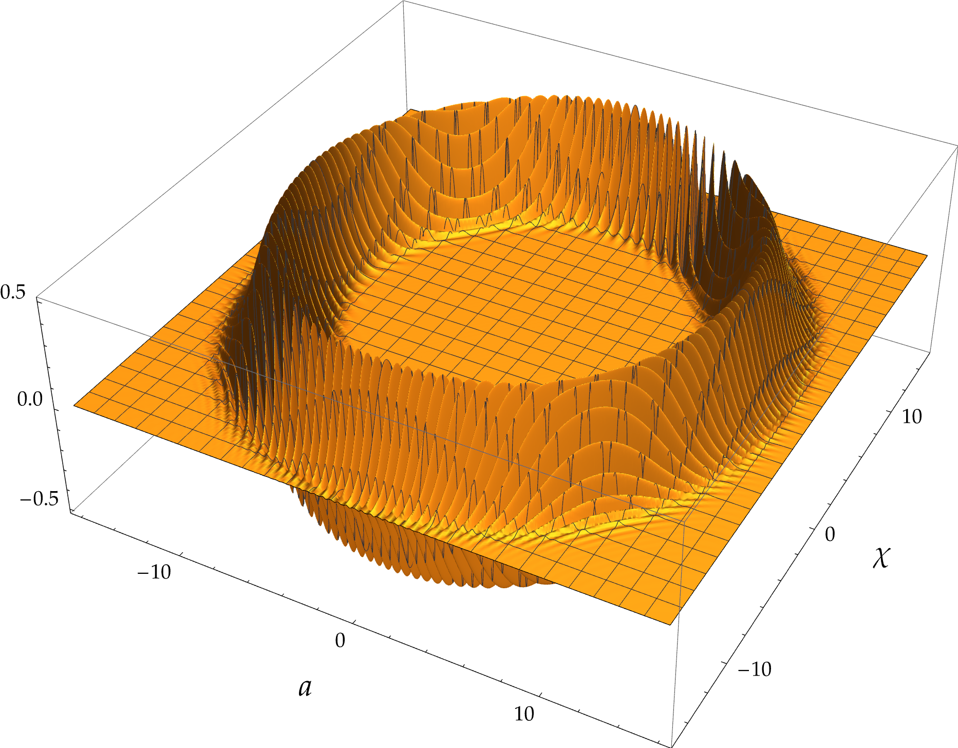
(a) $\beta=$1$$

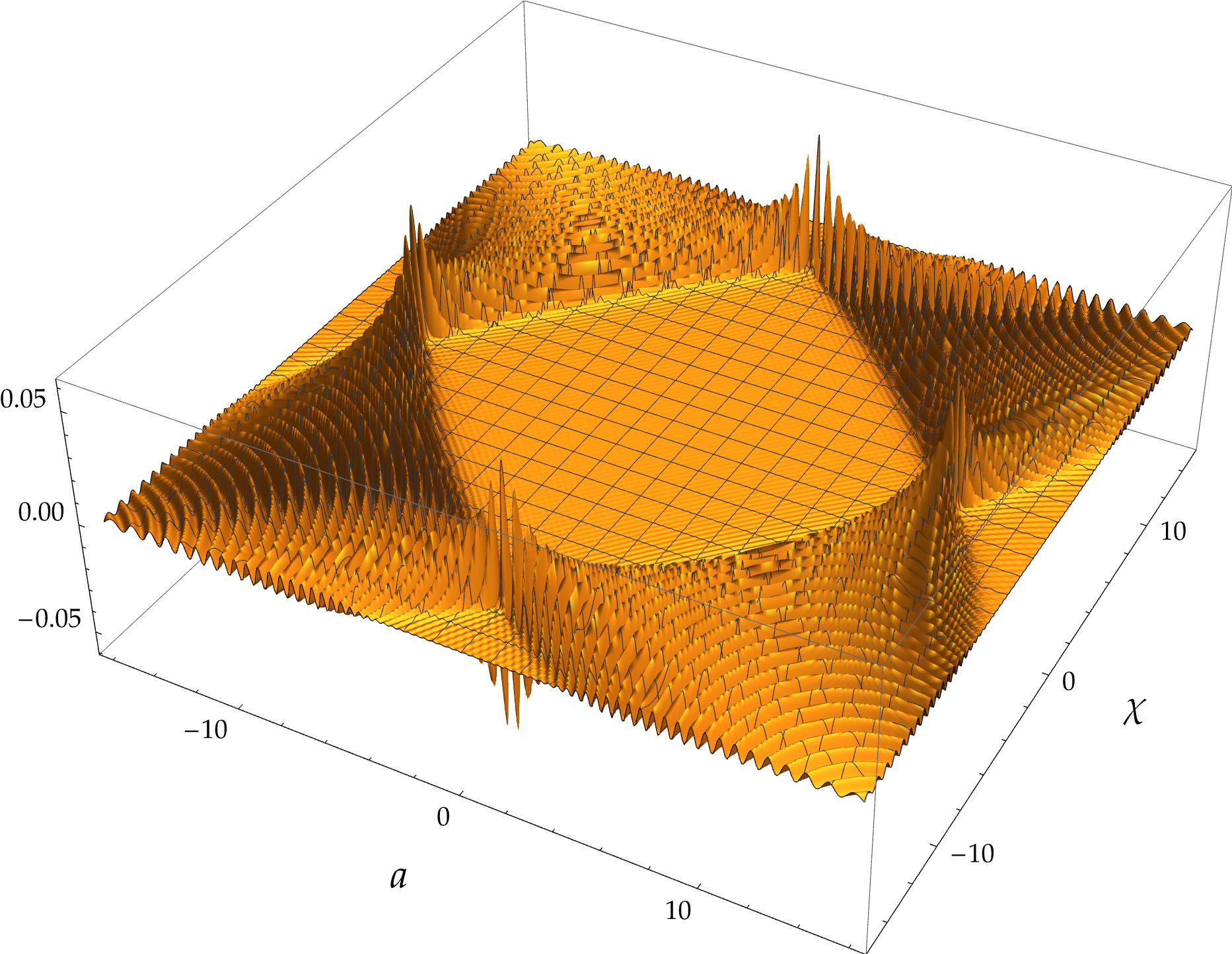
(b) $\beta=$0.03$$

Figure 1: Wave packets solving our toy model for time travel with $\omega_{\textsc{c}}=\omega_{\textsc{r}}$. Details regarding the construction of these solutions to the Hamiltonian constraint equation (20) can be found in appendix C. Left: Dispersion-less packets, corresponding to a parameter choice $\beta=1$. Right: Wave packets with strong dispersion, $\beta=0.03$.

As a preliminary, second step for the discussion of non-diagonal $A_{n,n^{\prime}}$, it is instructive to reexamine the commensurability condition. Plugging the ansatz (22) into the Hamiltonian constraint (20) we get for all values of $n$ and $n^{\prime}$ that

$$\left(\omega_{\textsc{c}}n+\frac{\omega_{\textsc{c}}}{2}-\omega_{\textsc{r}}n^{\prime}-\frac{\omega_{\textsc{r}}}{2}\right)A_{n,n^{\prime}}=0.$$ (33)

This implies that either $A_{n,n^{\prime}}=0$ or if $A_{n,n^{\prime}}\neq 0$ that

$$\left(\omega_{\textsc{c}}n+\frac{\omega_{\textsc{c}}}{2}-\omega_{\textsc{r}}n^{\prime}-\frac{\omega_{\textsc{r}}}{2}\right)=0,$$ (34)

which is equivalent to the original commensurability condition (21). Given that this condition yields a ratio of two odd numbers, we can rephrase $n$ and $n^{\prime}$ as

$$n=s(2p+1)+p;\qquad n^{\prime}=s(2q+1)+q;\qquad s,p,q\in\mathds{N}_{0}.$$ (35)

This equation gives additional insight about the coefficients $A_{n,n^{\prime}}$. In components, we can write

$$A_{n,n^{\prime}}=\sum_{s=0}^{\infty}\delta_{n,s(2p+1)+p}\;d_{s}\;\delta_{n^{\prime},s(2q+1)+q}$$ (36)

which in ‘matrix form’ appears as follows:

$$A=\Delta_{1}^{T}D\Delta_{2},$$ (37)

where $D$ really is diagonal and $\Delta_{1},\Delta_{2}$ are sparse matrices connecting $s$ with $n$ and $n^{\prime}$, respectively.

The third step takes a look at the numerator of the conditional probability of the PW formalism, equation (6). Note that equation (25) is fully general, and needed no diagonality of $A_{n,n^{\prime}}$ in its derivation. Its last two factors can now be evaluated with our general ansatz (22):

$$(\mathds{1}_{\textsc{c}}\otimes\hat{H}_{\textsc{r}})\ket{\Psi}=\sum_{n,n^{\prime}}A_{n,n^{\prime}}\left(n^{\prime}+\frac{1}{2}\right)\ket{n}_{\textsc{c}}\otimes\ket{n^{\prime}}_{\textsc{r}}.$$ (38)

As in the first step, we can then use orthonormality of the Fock states $\ket{n^{\prime}}_{\textsc{c,r}}$ and cyclicity of the trace to show that

$$\operatorname{tr}\left(\hat{H}_{\textsc{r}}\hat{P}_{\theta_{\ast}}\hat{\rho}\right)=\sum_{m,n,n^{\prime}}\left({\vphantom{\braket{m}{\psi({\theta}_{\ast})}}}_{\textsc{c}}\!\braket{m}{\psi(\theta_{\ast})}_{\textsc{c}}A_{m,n^{\prime}}^{*}\right)\left(A_{n,n^{\prime}}\left[n^{\prime}+\frac{1}{2}\right]\ {\vphantom{\braket{\psi({\theta}_{\ast})}{n}}}_{\textsc{c}}\!\braket{\psi(\theta_{\ast})}{n}_{\textsc{c}}\right).$$ (39)

Next, let us employ the definition of $\ket{\psi(\theta_{\ast})}_{\textsc{c}}$, equation (4):

$${\vphantom{\braket{m}{\psi({\theta}_{\ast})}}}_{\textsc{c}}\!\braket{m}{\psi(\theta_{\ast})}_{\textsc{c}} ={\vphantom{\ket{\psi({\theta}_{\ast})}}}_{\textsc{c}}\!\bra{m}e^{-i\hat{H}_{\textsc{c}}\theta_{\ast}}\ket{\psi(0_{\ast})}_{\textsc{c}},$$ (40)

$$=e^{-i(m+\frac{1}{2})\theta_{\ast}}\ {\vphantom{\braket{m}{\psi({0}_{\ast})}}}_{\textsc{c}}\!\braket{m}{\psi(0_{\ast})}_{\textsc{c}}.$$ (41)

This allows us to rearrange equation (39) to

$$\operatorname{tr}\left(\hat{H}_{\textsc{r}}\hat{P}_{\theta_{\ast}}\hat{\rho}\right)=\sum_{m,n}Q_{m,n}e^{+i(n-m)\theta_{\ast}}$$ (42)

where

$$Q_{m,n}\mathrel{\mathop{:}}=\left(\left[\sum_{n^{\prime}}A_{m,n^{\prime}}^{*}A_{n,n^{\prime}}(n^{\prime}+1/2)\right]\ {\vphantom{\braket{m}{\psi({0}_{\ast})}}}_{\textsc{c}}\!\braket{m}{\psi(0_{\ast})}_{\textsc{c}}\ {\vphantom{\braket{\psi({0}_{\ast})}{n}}}_{\textsc{c}}\!\braket{\psi(0_{\ast})}{n}_{\textsc{c}}\right)$$ (43)

This effectively demonstrates how the choice of the universe’s state $\ket{\Psi}$ and the chosen initial clock state $\ket{\psi(0_{\ast})}_{\textsc{c}}$ together fully determine the time evolution of our model. Equation (43) can equivalenty be expressed in ‘matrix form’ as

$$Q=D_{1}^{\dagger}A^{\dagger}D_{0}AD_{1},$$ (44)

where $D_{1}$ is a complex diagonal ‘matrix’, and $D_{0}$ a real diagonal ‘matrix’.

A closely related identity can also be found—using similar arguments—for the denominator of equation (6), reading:

$$\operatorname{tr}\left(\hat{P}_{\theta_{\ast}}\hat{\rho}\right)=\sum_{m,n}\left(\left[\sum_{n^{\prime}}A_{m,n^{\prime}}^{*}A_{n,n^{\prime}}\right]\;{\vphantom{\braket{m}{\psi({{0}_{\ast}})}}}_{\textsc{c}}\!\braket{m}{\psi(0_{\ast})}_{\textsc{c}}\ {\vphantom{\braket{\psi({0}_{\ast})}{n}}}_{\textsc{c}}\!\braket{\psi(0_{\ast})}{n}_{\textsc{c}}e^{+i(n-m)\theta_{\ast}}\right).$$ (45)

Note that this is again of the form (42), though with a simpler ‘$Q$’ for which $D_{0}=\mathds{1}$. This means any general statement that can be shown for $Q$ will hold for the corresponding part appearing in equation (45).

In our fourth and final step, we shall bring together our result (37) for $A_{n,n^{\prime}}$ and the result (44) for $Q_{m,n}$ to greatly constrain the conditional probabilities of equation (6). Concretely, inserting the former into the latter gives:

$$Q =D_{1}^{\dagger}(\Delta_{1}^{T}D\Delta_{2})^{\dagger}D_{0}(\Delta_{1}^{T}D\Delta_{2})D_{1},$$ (46)

$$=D_{1}^{\dagger}\Delta_{2}^{\dagger}D^{*}(\Delta_{1}^{*}D_{0}\Delta_{1}^{T})D\Delta_{2}D_{1}.$$ (47)

In this expression, let us investigate the central, bracketed term, $\Delta_{1}^{*}D_{0}\Delta_{1}^{T}$:

$$\left(\Delta_{1}^{*}D_{0}\Delta_{1}^{T}\right)_{ss^{\prime}} =\sum_{n^{\prime}}\delta_{n^{\prime},s(2q+1)+q}[D_{0}]_{n^{\prime}}\delta_{n^{\prime},s^{\prime}(2q+1)+q},$$ (48)

$$=\mathrel{\mathop{:}}(D_{3/2})_{ss^{\prime}},$$ (49)

another diagonal matrix. This in turn means that even more terms in the middle of equation (47) reduce to yet another diagonal matrix $D_{2}$, defined as

$$D_{2}\mathrel{\mathop{:}}=D^{*}(\Delta_{1}^{*}D_{0}\Delta_{1}^{T})D=D^{*}D_{3/2}D.$$ (50)

This, then, allows us to greatly simplify the structure of $Q$ itself:

$$Q=D_{1}^{\dagger}(\Delta_{2}^{\dagger}D_{2}\Delta_{2})D_{1},$$ (51)

whose middle part in brackets can, using the same approach as in equation (48), be shown to be diagonal. Finally, it follows that $Q$ itself is diagonal.

Essential for this result was the specific form of $A$, equation (37). Modifying the underlying model will therefore likely change this result. For the PW formalism in our context, though, the result is far-reaching: If we take equation (42), we see that for diagonal $Q$, the term $e^{i(n-m)\theta_{\ast}}=1$, as $n=m$. The same observation holds for the denominator of the PW conditional probabilities (6), equation (45). So, as in our first step when considering diagonal $A_{n,n^{\prime}}$, even the general case produces trivial time evolution.

At first glance, this seems a very unremarkable result, and therefore of little use for any interesting physics question. Ironically, this is not the case in our present situation, in which we are discussing time travel: An evolution that is simply constant is certainly still trivially a case of Novikov’s self-consistency conjecture. Given that nothing is happening, one might even go so far as to say that it gives an odd entry to the intersection of the Novikov self-consistency conjecture and the ‘boring physics conjecture’ Visser (1996). It is simultaneously both time travel and the absence of all evolution.

This result is also a marked departure from results in quantum cosmology Conradi and Zeh (1991); Brunetti et al. (2010). The reason for this disparity is the limited domain of the scale parameter in the models of the form (20). Most importantly, limiting a harmonic oscillator to half of its configuration space will prevent the application of ladder operators as we used them in the above analysis. This again demonstrates how ‘simple’ changes to the model can quite radically change results.

5 Interpretation, Discussion and Outlook

Despite the disappointingly boring outcome for our particular model, our toy model serves its purpose as a proof-of-concept study. It demonstrates the feasibility for future model building of quantum systems with periodic, emergent notions of time as a tool to study time travel. The obvious model-dependence of the PW formalism through its dependence on $\ket{\Psi}$, the ‘state of the universe’, means that different models might have very different conclusions as to what sort of time evolution is possible. As even collections of harmonic oscillators become increasingly complex once interactions start to enter, necessitating many different heuristics or approaches across fields Auletta et al. (2009); Zee (2010), it is unlikely that the PW formalism can be fully general even when discussing whether time travel is possible based on first principles of quantum theory.

In the absence of a fully general result, we still believe that some general conclusions can nevertheless be achieved. Analytically tractable models beyond the one presented in our study should be possible, especially given that POVMs and the PW formalism feature prominently in the modern, gauge theoretic consolidation of emergent time in quantum theory. The use of POVMs in future extensions was part of the motivation to highlight them as much in our discussion as we did, despite the final result not relying on them.

The goals of such a future model building task would contain the following:

• More and different subsystems; more in the sense of more harmonic oscillators, different in adding various combinations of other systems. Also ancillary systems could be used. For example, in the context of time travel, one can ask the following question: Can ancillary or memory systems allow for (more or less self-consistent) time travel being limited to just a fixed, finite number of round trips as opposed to the infinite traversability of GR’s CTCs?

• In a closely related step, one would introduce various interactions among the subsystems. These will greatly change the outcome of our above analysis.

• Ultimately, the combination of these two model building drives can try to investigate entropic arguments in the context of time travel. If self-consistent time travel in quantum systems with an emergent notion of time is possible, are such configurations potentially favoured or disfavoured on thermodynamic grounds? In particular, entropy concepts geared towards constrained or fixed energy systems, like ‘observational entropy’ Šafránek et al. (2019a, b, 2021), promise access to new arguments for or against time travel without having to rely on either mixing different concepts of time (GR’s dynamic time vs. thermodynamic time vs. parameter time vs. …) or, in fact, without relying on any kind of explicit notion of time; the entropic arguments in such systems would similarly be based on emergent notions, just as the notion of time itself is.

• Similarly, this exercise should be able to further clarify the difference between a periodic clock time and time travel as such. Obviously, some kind of synchronicity between residual system and clock system has to hold for the latter. Yet the above mentioned research directions would allow one to turn concepts like self-consistency into less of a binary. After all, if time is emergent, its absence might be ill-suited for human survival but still allow a valid physical system that describes something ‘close’ to a quantum system with self-consistent, observable time travel. In a sense, this would be a first step towards rigorously testing Hawking’s chronology protection.

• Much of the current research which led to a reimagining of the PW formalism as a gauge fixed picture aims to ask what happens when one changes frames, i.e., clocks. Once the model systems for time travel are complex enough (and, thus, more complex than our equation (20)), a natural question is: What happens to time travel in such quantum reference frame transformations? And, linking to the previous point, does this differ from the situation for merely periodic clocks?

• Lastly, the previous two points hint at the possibility of making time travel more a local, emergent notion in a large system. This is, for one, the explicit way to study time travel classically as CTCs in a space-time manifold, see, for example, Earman et al. (2009); Dolanský and Krtouš (2010). For another, this is similarly done in quantum physics, ranging from the rigorously and explicitly local Bishop et al. (2021); Alonso-Serrano et al. (2021) to the more imprecise and only implicitly local Deutsch (1991); Lloyd et al. (2011). Yet, so far, these approaches all had to rely on an ad-hoc introduction of ‘background’ time.

There are other avenues along similar lines that warrant a closer look in the framework of quantum gravity. In the canonical approach to it, for instance, different inner products can be considered, so at least changing the mathematical framework drastically—begging the question how much of the physical interpretation changes or has to change in tandem. Other approaches to quantum gravity besides the canonical ones can also test emergent notions of time in their respective frameworks. Besides a question of tractability, this was part of the motivation to keep our toy model somewhat agnostic and conservative with respect to a theory of quantum gravity.

Independent of which direction one would want to take, we believe that our first result shows that emergent notions of time in quantum physics can lead to a multitude of questions and interpretational conundra pertaining to time travel. The very introduction of such an emergent time concepts undermines most traditional arguments against time travel. The concepts evoked in these arguments simply have to rely on notions that are not valid in more ab initio approaches.

A.A.-S. is funded by the Deutsche Forschungsgemeinschaft (DFG, German Research Foundation) — Project ID 516730869. This work was also partially supported by Spanish Project No. MICINN PID2020-118159GB-C41. S.S. was financially supported by Czech Science Foundation grant GACR 23-07457S. M.V. was directly supported by the Marsden Fund, via a grant administered by the Royal Society of New Zealand.

No new data were created or analyzed in this study. Data sharing is not applicable to this article.

Appendix A Formal Definition of POVMs

Let us present in this appendix the formal definition of a POVM. An operator $\hat{A}$ on a Hilbert space $\mathcal{H}$ is called positive, if

$$\forall\ket{\psi}\in\mathcal{H}:\qquad\braket{\psi}{\hat{A}}{\psi}\geq 0.$$ (52)

Positivity of an operator is often denoted as ‘$\hat{A}\geq 0$.’ An operator $B$ is called a POVM if and only if it is an additive map from a Borel $\sigma$-algebra $\mathcal{A}$ of subsets of a set $\Omega$ to operators on $\mathcal{H}$ such that

• for all sets $X\in\mathcal{A}$, $B(X)\geq 0$ (‘positivity’),

• for disjoint $X,Y\in\mathcal{A}$, $B(X\cup Y)=B(X)+B(Y)$ (‘additivity’),

• for all sequences of sets $X_{n}\in\mathcal{A}$ such that $\cap_{n=1}^{\infty}X_{n}=\emptyset$, all operators $B(X_{n})$ have $\hat{0}$ (the zero operator) as greatest lower bound.

For more details, see (Busch et al., 2016, p.71, Def.4.5). A POVM that fulfils $B(\Omega)=\mathds{1}$ is called normalized.

Normalized POVMs are a more general notion of observable compared to that of observables being unbounded, self-adjoint operators on $\mathcal{H}$. The (set-theoretic) ‘universe’ $\Omega$ corresponds to possible measurement outcomes. In this sense, additivity and being normalized links measurements as described by POVMs to the theory of probablity as set down in the Kolmogorov axioms. They allow for more and wider notions of imprecision than those encoded in density matrices Auletta et al. (2009); Busch et al. (2016). In ‘standard quantum mechanics,’ The measurement process of an observable $\hat{A}$ according to the Born rule projects onto a subspace formed by eigenvectors of $\hat{A}$ with set eigenvalue $A_{i}$. In the terminology of POVMs this corresponds to ‘projection-valued measures’ (PVMs), and PVMs $\subsetneq$ POVMs.

Appendix B Time Operators for a Harmonic Oscillator

In this appendix, we want to draw attention to some additional background regarding POVMs and phase or time operators in the context of harmonic oscillators.

With the POVM $B_{0}$ of equation (15) in place, we can now define a large number of new, self-adjoint operators Busch et al. (1994). To do this, we associate to each real-valued, bounded, and measurable function $f$ on $[0,2\pi)$ the operator $\hat{B}_{0}[f]$ defined as

$$\hat{B}_{0}[f] \mathrel{\mathop{:}}=\frac{1}{2\pi}\int_{0}^{2\pi}f(\theta)\ket{\theta}\negthickspace\bra{\theta}\operatorname{d}\!\theta,$$ (53)

$$=\sum_{n,m\geq 0}\frac{1}{2\pi}\int_{0}^{2\pi}e^{i(n-m)\theta}f(\theta)\ket{n}\negthickspace\bra{m}\operatorname{d}\!\theta.$$ (54)

This procedure fixes the set $X$ in the original POVM $B_{0}$, and then uses it to construct various Toeplitz operators. Different choices for $f$ can be found in the literature (see, for example, Garrison and Wong (1970)), but we will focus on one of the simplest options:

$$f(\theta)=\theta.$$ (55)

This will give us a time operator $\hat{T}_{0}$, which we calculate with the above expressions to be

$$\hat{T}_{0}=\hat{B}_{0}[\theta]=\sum_{n\neq m\geq 0}\frac{1}{i(n-m)}\ket{n}\negthickspace\bra{m}+\pi\mathds{1}.$$ (56)

However, this operator is not unique. First of all, we could have chosen a different starting point for our angles, changing the index $0$ at that point. There is also a different, but more physically motivated point of arriving at additional time operators. The time operator $\hat{T}_{0}$ can be covariantly shifted to a new operator $\hat{T}_{\theta_{\ast}}$:

$$\hat{T}_{\theta_{\ast}}\mathrel{\mathop{:}}=e^{i\hat{H}\theta_{\ast}}\hat{T}_{0}e^{-i\hat{H}\theta_{\ast}}.$$ (57)

This covariant shift property is a general feature of such time operators from POVMs, see Busch et al. (1994), that is increasingly prominent and clear in their modern implementations Höhn et al. (2021a); Smith (2019). Importantly, while all such $\hat{T}_{\theta_{\ast}}$ fulfil canonical commutation relations with $\hat{H}$ (when the resulting operator is well-defined), different time operators will not commute with each other:

$$\theta_{\ast}\neq\theta_{\ast}^{\prime}\mod 2\pi\qquad\Longrightarrow\qquad[\hat{T}_{\theta_{\ast}}\hat{T}_{\theta_{\ast}^{\prime}}]\neq 0.$$ (58)

These results deserve some commentary. The reason why these time operators are still self-adjoint, despite the illustrious list of no-go theorems given in the introduction, is two-fold Busch et al. (1994): One, they are hardly unique. Any change in starting point (phase) will yield a different time operator. A covariant shift similarly yields new time operators. Two, the domain of time is now periodic. The no-go theorems usually aim for $\mathds{R}$ as domain for time $\theta$, or that the time would be unique in some sense. In the present context, it is more a question of when one started the periodic clock, and what period the clock has. It is also worth pointing out that our time operators subtly fail to satisfy the expected time-energy uncertainty: It will not hold for all states in $\mathcal{H}$, but only for a densely defined set Garrison and Wong (1970); Galindo (1984). This latter restriction is not an issue for our purposes, at least in the present article, and the other reasons for evading the no-go theorems are what allows our application in the context of time travel.

Appendix C Detailed Construction of Depicted Wave Packets

For our figure 1, we adapted the plots of Kiefer (1990) to our present context with a larger configuration space. For ease of comparison, we kept the notation for the wave functions the same. We do, however, emphasize that in our context one should not interpret $a$ as a scale factor. Our investigation is not quantum cosmology, just inspired by a particular model of it due to its simplicity.

A general solution of equation (20) can be expressed in configuration space variables $a,\chi$ instead of the Fock space picture adapted in the remainder of the article. For illustration purposes, this is preferable. We will restrict attention to symmetric wavefunctions, in which $a$ and $\chi$ can be assigned equally well to the clock system $\hat{H}_{\textsc{c}}$ or the residual system $\hat{H}_{\textsc{r}}$. While our enlarged configuration space (compared to that of quantum cosmology) might change the overall normalization, it will not change the qualitative behaviour of the wavefunctions. We therefore also copy the normalization of reference Kiefer (1990).

A wavefunction with two Gaussians centered around $\chi=\pm\chi_{0}$, each of width $\beta$, at time/position $a=0$, is given by

$$\Psi(a,\chi)=\sum_{m=0}^{\infty}c_{2m}\frac{H_{2m}(a)H_{2m}(\chi)}{\sqrt{2^{2m}(2m)!}H_{2m}(0)}\exp\left(-\frac{1}{2}a^{2}-\frac{1}{2}\chi^{2}\right),$$ (59)

where $H_{n}(x)$ is the $n$-th Hermite polynomial and the expansion coefficients are

$$c_{n}=\frac{1}{\sqrt{2^{n}n!}}\sqrt{\frac{2\beta}{1+\beta^{2}}}\exp\left(-\frac{\chi_{0}^{2}}{2(1+\beta^{2})}\right)\left(\sqrt{\frac{1-\beta^{2}}{1+\beta^{2}}}\right)^{n}H_{n}\left(\frac{\chi_{0}}{\sqrt{1-\beta^{4}}}\right).$$ (60)

These coefficients $c_{n}$ simplify further for the ‘coherent case’, i.e., when $\beta=1$, to

$$c_{n}=\exp\left(-\frac{1}{4}\chi_{0}^{2}\right)\frac{\chi_{0}^{n}}{\sqrt{2^{n}n!}}.$$ (61)

Note that the index $m$ in equation (59) is meant to make more explicit that the sum runs only over even $n$.

References

References

- Roman (1993) Roman, T.A. Inflating Lorentzian wormholes. Physical Review D 1993, 47, 1370–1379, [arXiv:gr-qc/9211012 [gr-qc]]. https://doi.org/10.1103/PhysRevD.47.1370.
- Krasnikov (2002) Krasnikov, S. No time machines in classical general relativity. Classical and Quantum Gravity 2002, 19, 4109–4129, [arXiv:gr-qc/0111054 [gr-qc]]. Erratum in Classical and Quantum Gravity 2014 31(7), 079503. https://doi.org/10.1088/0264-9381/31/7/079503, https://doi.org/10.1088/0264-9381/19/15/316.
- Visser (1997) Visser, M. The reliability horizon for semi-classical quantum gravity: Metric fluctuations are often more important than back-reaction. Physics Letters B 1997, 415, 8–14, [arXiv:gr-qc/9702041 [gr-qc]]. https://doi.org/10.1016/S0370-2693(97)01226-4.
- Hawking (1992) Hawking, S.W. Chronology protection conjecture. Physical Review D 1992, 46, 603–611. https://doi.org/10.1103/PhysRevD.46.603.
- Klinkhammer (1992) Klinkhammer, G. Vacuum polarization of scalar and spinor fields near closed null geodesics. Physical Review D 1992, 46, 3388–3394. https://doi.org/10.1103/PhysRevD.46.3388.
- Visser (1993) Visser, M. From wormhole to time machine: Remarks on Hawking’s chronology protection conjecture. Physical Review D 1993, 47, 554–565, [arXiv:hep-th/9202090 [hep-th]]. https://doi.org/10.1103/PhysRevD.47.554.
- Emparan and Tomašević (2022) Emparan, R.; Tomašević, M. Quantum backreaction on chronology horizons. Journal of High Energy Physics 2022, 02, 182, [arXiv:2109.03611 [hep-th]]. https://doi.org/10.1007/JHEP02(2022)182.
- Pons et al. (2010) Pons, J.M.; Sundermeyer, K.A.; Salisbury, D.C. Observables in classical canonical gravity: folklore demystified. Journal of Physics: Conference Series 2010, 222, 012018, [arXiv:1001.2726 [gr-qc]]. https://doi.org/10.1088/1742-6596/222/1/012018.
- Anderson (2017) Anderson, E. The Problem of Time; Vol. 190, Fundamental Theories of Physics, Springer, 2017. https://doi.org/10.1007/978-3-319-58848-3.
- Kiefer and Peter (2022) Kiefer, C.; Peter, P. Time in Quantum Cosmology. Universe 2022, 8, 36, [arXiv:2112.05788 [gr-qc]]. https://doi.org/10.3390/universe8010036.
- Mandelstam and Tamm (1945) Mandelstam, L.I.; Tamm, I.Y. The uncertainty relation between energy and time in nonrelativistic quantum mechanics. Journal of Physics 1945, IX, 249–254. English translation of Л. И. Мандельштам, И. Е. Тамм “Соотношение неопределённости энергия-время внерелятивистской квантовой механике”, Изв. Дкад. Наук СССР (сер. физ.) 9, 122–128 (1945).
- Schrödinger (1931) Schrödinger, E. Spezielle Relativitätstheorie und Quantenmechanik. Sitzungsberichte der Preußischen Akademie der Wissenschaften. Physikalisch-mathematische Klasse 1931, pp. 238–247.
- Pauli (1990) Pauli, W. Die allgemeinen Prinzipien der Wellenmechanik; Springer, 1990. Neu herausgegeben und mit historischen Anmerkungen versehen von Norbert Straumann, https://doi.org/10.1007/978-3-642-62187-9.
- Pauli (1980) Pauli, W. General Principles of Quantum Mechanics; Springer, 1980. English translation of Pauli (1990), https://doi.org/10.1007/978-3-642-61840-6.
- Unruh and Wald (1989) Unruh, W.G.; Wald, R.M. Time and the interpretation of canonical quantum gravity. Physical Review D 1989, 40, 2598–2614. https://doi.org/10.1103/PhysRevD.40.2598.
- Böhm (1993) Böhm, A. Quantum Mechanics – Foundations and Applications, third ed.; Springer, 1993.
- de la Madrid et al. (2002) de la Madrid, R.; Böhm, A.; Gadella, M. Rigged Hilbert Space Treatment of Continuous Spectrum. Fortschritte der Physik 2002, 50, 185–216, [quant-ph/0109154]. https://doi.org/10.1002/1521-3978(200203)50:2<185::AID-PROP185>3.0.CO;2-S.
- Thiemann (2008) Thiemann, T. Modern Canonical Quantum General Relativity; Cambridge Monographs on Mathematical Physics, Cambridge University Press, 2008.
- Busch et al. (2016) Busch, P.; Lahti, P.; Pellonpää, J.P.; Ylinen, K. Quantum Measurement; Theoretical and Mathematical Physics, Springer, 2016.
- Fewster and Verch (2020) Fewster, C.J.; Verch, R. Quantum Fields and Local Measurements. Communications in Mathematical Physics 2020, 378, 851–889, [arXiv:1810.06512 [math-ph]]. https://doi.org/10.1007/s00220-020-03800-6.
- Busch et al. (1995) Busch, P.; Grabowski, M.; Lahti, P.J. Who Is Afraid of POV Measures? Unified Approach to Quantum Phase Observables. Annals of Physics 1995, 237, 1–11. https://doi.org/10.1006/aphy.1995.1001.
- Auletta et al. (2009) Auletta, G.; Fortunato, M.; Parisi, G. Quantum Mechanics; Cambridge University Press, 2009.
- Busch et al. (1994) Busch, P.; Grabowski, M.; Lahti, P.J. Time observables in quantum theory. Physics Letters A 1994, 191, 357–361. https://doi.org/10.1016/0375-9601(94)90785-4.
- Einstein (1905) Einstein, A. Zur Elektrodynamik bewegter Körper. Annalen der Physik 1905, 322, 891–921. https://doi.org/10.1002/andp.19053221004.
- DeWitt (1967) DeWitt, B.S. Quantum Theory of Gravity. 1. The Canonical Theory. Physical Review 1967, 160, 1113–1148. https://doi.org/10.1103/PhysRev.160.1113.
- Page and Wootters (1983) Page, D.N.; Wootters, W.K. Evolution without evolution: Dynamics described by stationary observables. Physical Review D 1983, 27, 2885–2892. https://doi.org/10.1103/PhysRevD.27.2885.
- Wootters (1984) Wootters, W.K. “Time” replaced by quantum correlations. International Journal of Theoretical Physics 1984, 23, 701–711. https://doi.org/10.1007/BF02214098.
- Kuchař (2011) Kuchař, K.V. Time and Interpretations of Quantum Gravity. International Journal of Modern Physics D 2011, 20, 3–86. Contribution to: 4th Canadian Conference on General Relativity and Relativistic Astrophysics, https://doi.org/10.1142/S0218271811019347.
- Giovannetti et al. (2015) Giovannetti, V.; Lloyd, S.; Maccone, L. Quantum Time. Physical Review D 2015, 92, 045033, [arXiv:1504.04215 [quant-ph]]. https://doi.org/10.1103/PhysRevD.92.045033.
- Marletto and Vedral (2017) Marletto, C.; Vedral, V. Evolution without evolution, and without ambiguities. Physical Review D 2017, 95, 043510, [arXiv:1610.04773 [quant-ph]]. https://doi.org/10.1103/PhysRevD.95.043510.
- Gemsheim and Rost (2023) Gemsheim, S.; Rost, J.M. Emergence of Time from Quantum Interaction with the Environment. Physical Review Letters 2023, 131, 140202, [arXiv:2309.05159 [quant-ph]]. https://doi.org/10.1103/PhysRevLett.131.140202.
- Smith and Ahmadi (2019) Smith, A.R.H.; Ahmadi, M. Quantizing time: Interacting clocks and systems. Quantum 2019, 3, 160, [arXiv:1712.00081 [quant-ph]]. https://doi.org/10.22331/q-2019-07-08-160.
- Höhn et al. (2021a) Höhn, P.A.; Smith, A.R.H.; Lock, M.P.E. The Trinity of Relational Quantum Dynamics. Physical Review D 2021, 104, 066001, [arXiv:1912.00033 [quant-ph]]. https://doi.org/10.1103/PhysRevD.104.066001.
- Höhn et al. (2021b) Höhn, P.A.; Smith, A.R.H.; Lock, M.P.E. Equivalence of Approaches to Relational Quantum Dynamics in Relativistic Settings. Frontiers in Physics 2021, 9, 181, [arXiv:2007.00580 [gr-qc]]. https://doi.org/10.3389/fphy.2021.587083.
- Krumm et al. (2021) Krumm, M.; Höhn, P.A.; Müller, M.P. Quantum reference frame transformations as symmetries and the paradox of the third particle. Quantum 2021, 5, 530, [arXiv:2011.01951 [quant-ph]]. https://doi.org/10.22331/q-2021-08-27-530.
- Goeller et al. (2022) Goeller, C.; Höhn, P.A.; Kirklin, J. Diffeomorphism-invariant observables and dynamical frames in gravity: reconciling bulk locality with general covariance 2022. [arXiv:2206.01193 [hep-th]].
- Adlam (2022) Adlam, E. Watching the Clocks: Interpreting the Page–Wootters Formalism and the Internal Quantum Reference Frame Programme. Foundations of Physics 2022, 52, 99, [arXiv:2203.06755 [physics.hist-ph]]. https://doi.org/10.1007/s10701-022-00620-7.
- Höhn et al. (2023) Höhn, P.A.; Russo, A.; Smith, A.R.H. Matter relative to quantum hypersurfaces 2023. [arXiv:2308.12912 [quant-ph]].
- Hausmann et al. (2023) Hausmann, L.; Schmidhuber, A.; Castro-Ruiz, E. Measurement events relative to temporal quantum reference frames 2023. [arXiv:2308.10967 [quant-ph]].
- Höhn et al. (2023) Höhn, P.A.; Kotecha, I.; Mele, F.M. Quantum Frame Relativity of Subsystems, Correlations and Thermodynamics 2023. [arXiv:2308.09131 [quant-ph]].
- Deutsch (1991) Deutsch, D. Quantum mechanics near closed timelike lines. Physical Review A 1991, 44, 3197–3217. https://doi.org/10.1103/PhysRevD.44.3197.
- Bishop et al. (2021) Bishop, L.G.; Costa, F.; Ralph, T.C. Time-travelling billiard-ball clocks: a quantum model. Physical Review A 2021, 103, 042223, [arXiv:2007.12677 [quant-ph]]. https://doi.org/10.1103/PhysRevA.103.042223.
- Baumann et al. (2022) Baumann, V.; Krumm, M.; Guérin, P.A.; Časlav Brukner. Noncausal Page–Wootters circuits. Physical Review Research 2022, 4, 013180, [arXiv:2105.02304 [quant-ph]]. https://doi.org/10.1103/PhysRevResearch.4.013180.
- Vilasini (2021) Vilasini, V. Approaches to causality and multi-agent paradoxes in non-classical theories. PhD thesis, University of York, 2021, [arXiv:2102.02393 [quant-ph]].
- Adlam (2022) Adlam, E. Two roads to retrocausality. Synthese 2022, 200, 422, [arXiv:2201.12934 [physics.hist-ph]]. https://doi.org/10.1007/s11229-022-03919-0.
- Barceló et al. (2022) Barceló, C.; Sánchez, J.E.; García-Moreno, G.; Jannes, G. Chronology protection implementation in analogue gravity. European Physical Journal C 2022, 82, 299, [2201.11072]. https://doi.org/10.1140/epjc/s10052-022-10275-3.
- Sabín (2022) Sabín, C. Analogue Non-Causal Null Curves and Chronology Protection in a dc-SQUID Array. Universe 2022, 8, 452, [arXiv:quant-ph/2207.14164]. https://doi.org/10.3390/universe8090452.
- Zeh (2007) Zeh, H.D. The Physical Basis of the Direction of Time, fifth ed.; The Frontiers Collection, Springer, 2007. https://doi.org/10.1007/978-3-540-68001-7.
- Truesdell (1971) Truesdell, C. Tragicomedy of Classical Thermodynamics; Springer, 1971.
- Minguzzi and Sánchez (2006) Minguzzi, E.; Sánchez, M. The causal hierarchy of spacetimes. In Recent developments in pseudo-Riemannian geometry; Baum, H.; Alekseevsky, D., Eds.; EMS Publishing House, 2006; p. 299–358, [arXiv:gr-qc/0609119 [gr-qc]].
- Barcelo and Visser (2002) Barcelo, C.; Visser, M. Twilight for the energy conditions? International Journal of Modern Physics D 2002, 11, 1553–1560, [arXiv:gr-qc/0205066 [gr-qc]]. https://doi.org/10.1142/S0218271802002888.
- Earman et al. (2009) Earman, J.; Smeenk, C.; Wüthrich, C. Do the laws of physics forbid the operation of time machines? Synthese 2009, 169, 91–124. https://doi.org/10.1007/s11229-008-9338-2.
- Manchak (2009) Manchak, J.B. On the Existence of “Time Machines” in General Relativity. Philosophy of Science 2009, 76, 1020–1026. https://doi.org/10.1086/605806.
- Manchak (2018) Manchak, J.B. Some “No Hole” Spacetime Properties are Unstable. Foundations of Physics 2018, 48, 1539–1545. https://doi.org/10.1007/s10701-018-0211-y.
- Manchak (2021) Manchak, J.B. General Relativity as a Collection of Collections of Models. In Hajnal Andréka and István Németi on the Unity of Science: From Computing to Relativity Theory Through Algebraic Logic; Madarász, J.; Székely, G., Eds.; Springer, 2021; Vol. 19, Outstanding Contributions to Logic, chapter 19, pp. 409–425. https://doi.org/10.1007/978-3-030-64187-0_17.
- Santiago et al. (2022) Santiago, J.; Schuster, S.; Visser, M. Generic warp drives violate the null energy condition. Physical Review D 2022, 105, 064038, [arXiv:2105.03079 [gr-qc]]. https://doi.org/10.1103/PhysRevD.105.064038.
- González-Díaz and Alonso-Serrano (2011) González-Díaz, P.F.; Alonso-Serrano, A. Observing other universe through ringholes and Klein-bottle holes. Physical Review D 2011, 84, 023008, [arXiv:1102.3784 [astro-ph.CO]]. https://doi.org/10.1103/PhysRevD.84.023008.
- Everett (1996) Everett, A.E. Warp drive and causality. Physical Review D 1996, 53, 7365. https://doi.org/10.1103/PhysRevD.53.7365.
- Gödel (1949) Gödel, K. An Example of a New Type of Cosmological Solutions of Einstein’s Field Equations of Gravitation. Review of Modern Physics 1949, 21, 447–450. https://doi.org/10.1103/RevModPhys.21.447.
- Hawking and Ellis (1974) Hawking, S.W.; Ellis, G.F.R. The large scale structure of space-time; Cambridge Monographs on Mathematical Physics, Cambridge University Press, 1974. https://doi.org/10.1017/CBO9780511524646.
- Griffiths and Podolský (2012) Griffiths, J.B.; Podolský, J. Exact Space-Times in Einstein’s General Relativity, first paperback ed.; Cambridge Monographs on Mathematical Physics, Cambridge University Press, 2012.
- Gray et al. (2017) Gray, F.; Santiago, J.; Schuster, S.; Visser, M. “Twisted” black holes are unphysical. Modern Physics Letters A 2017, 32, 1771001, [1610.06135]. https://doi.org/10.1142/S0217732317710018.
- Wald (1984) Wald, R.M. General Relativity; The University of Chicago Press, 1984.
- Penrose (1972) Penrose, R. Techniques of Differential Topology in General Relativity; Society for Industrial & Applied, 1972.
- Krasnikov (1998) Krasnikov, S. Hyperfast Interstellar Travel in General Relativity. Physical Review D 1998, 57, 4760–4766, [arXiv:gr-qc/9511068 [gr-qc]]. https://doi.org/10.1103/PhysRevD.57.4760.
- Manchak (2011) Manchak, J.B. No no-go: A remark on time machines. Studies in History and Philosophy of Modern Physics 2011, 42, 74–76. https://doi.org/10.1016/j.shpsb.2011.01.001.
- Novikov (1992) Novikov, I.D. Time machine and selfconsistent evolution in problems with selfinteraction. Physical Review D 1992, 45, 1989–1994. https://doi.org/10.1103/PhysRevD.45.1989.
- Sklar (1990) Sklar, L. How Free are Initial Conditions? In Proceedings of the Proceedings of the Biennial Meeting of the Philosophy of Science Association Vol. 1990, Volume Two: Symposia and Invited Papers. University of Chicago Press, 1990, pp. 551–564. https://doi.org/10.1086/psaprocbienmeetp.1990.2.193097.
- Friedman et al. (1990) Friedman, J.; Morris, M.S.; Novikov, I.D.; Echeverria, F.; Klinkhammer, G.; Thorne, K.S.; Yurtsever, U. Cauchy problem in spacetimes with closed timelike curves. Physical Review D 1990, 42, 1915–1930. https://doi.org/10.1103/PhysRevD.42.1915.
- Kiefer (2012) Kiefer, C. Quantum Gravity, 3rd ed.; Vol. 136, International Series of Monographs on Physics, Oxford University Press, 2012.
- Echeverria et al. (1991) Echeverria, F.; Klinkhammer, G.; Thorne, K.S. Billiard balls in wormhole space-times with closed timelike curves: Classical theory. Physical Review D 1991, 44, 1077–1099. https://doi.org/10.1103/PhysRevD.44.1077.
- Fewster et al. (1996) Fewster, C.J.; Higuchi, A.; Wells, C.G. Classical and Quantum Initial Value Problems for Models of Chronology Violation. Physical Review D 1996, 54, 3806, [arXiv:gr-qc/9603045 [gr-qc]]. https://doi.org/10.1103/PhysRevD.54.3806.
- Bachelot (2002) Bachelot, A. Global properties of the wave equation on non-globally hyperbolic manifolds. Journal de Mathématique Pures et Appliquées 2002, 81, 35–65. https://doi.org/10.1016/S0021-7824(01)01229-6.
- Dolanský and Krtouš (2010) Dolanský, J.; Krtouš, P. Billiard in the space with a time machine. Physical Review D 2010, 82, 124056, [arXiv:1011.2881 [gr-qc]]. https://doi.org/10.1103/PhysRevD.82.124056.
- Susskind and Glogower (1964) Susskind, L.; Glogower, J. Quantum mechanical phase and time operator. Physics Physique Fizika 1964, 1, 49–61. https://doi.org/10.1103/PhysicsPhysiqueFizika.1.49.
- Garrison and Wong (1970) Garrison, J.C.; Wong, J. Canonically Conjugate Pairs, Uncertainty Relations, and Phase Operators. Journal of Mathematical Physics 1970, 11, 2242–2249. https://doi.org/10.1063/1.1665388.
- Galindo (1984) Galindo, A. Phase and Number. Letters in Mathematical Physics 1984, 8, 495–500. https://doi.org/10.1007/BF00400979.
- Reed and Simon (1980) Reed, M.; Simon, B. Methods of Modern Mathematical Physics: I. Functional Analysis, revised and enlarged ed.; Academic Press, 1980.
- Kiefer (1989) Kiefer, C. Non-minimally coupled scalar fields and the initial value problem in quantum gravity. Physics Letters B 1989, 225, 227–232. https://doi.org/10.1016/0370-2693(89)90810-1.
- Kiefer (1990) Kiefer, C. Wave packets in quantum cosmology and the cosmological constant. Nuclear Physics B 1990, 341, 273–293. https://doi.org/10.1016/0550-3213(90)90271-E.
- Page (1991) Page, D.N. Minisuperspaces with conformally and minimally coupled scalar fields. Journal of Mathematical Physics 1991, 32, 3427–3438. https://doi.org/10.1063/1.529457.
- Brunetti et al. (2010) Brunetti, R.; Fredenhagen, K.; Hoge, M. Time in Quantum Physics: From an External Parameter to an Intrinsic Observable. Foundation of Physics 2010, 40, 1368–1378, [arXiv:0909.1899 [math-ph]]. https://doi.org/10.1007/s10701-009-9400-z.
- Hawking and Ellis (1965) Hawking, S.W.; Ellis, G.F.R. Singularities in homogeneous world models. Physics Letters 1965, 17, 246–247. Typo in first author of published version., https://doi.org/10.1016/0031-9163(65)90510-X.
- O’Neill (1983) O’Neill, B. Semi-Riemannian Geometry with Applications to Relativity; Pure and Applied Mathematics, Academic Press, 1983.
- Visser (1996) Visser, M. Lorentzian Wormholes: From Einstein to Hawking; AIP Series in Computational and Applied Mathematical Physics, American Institute of Physics, 1996.
- Conradi and Zeh (1991) Conradi, H.D.; Zeh, H.D. Quantum cosmology as an initial value problem. Physics Letters A 1991, 154, 321–326. https://doi.org/10.1016/0375-9601(91)90026-5.
- Zee (2010) Zee, A. Quantum Field Theory in a Nutshell, second ed.; Princeton University Press, 2010.
- Šafránek et al. (2019a) Šafránek, D.; Deutsch, J.M.; Aguirre, A. Quantum coarse-grained entropy and thermodynamics. Physical Review A 2019, 99, 010101, [arXiv:1707.09722 [quant-ph]]. https://doi.org/10.1103/PhysRevA.99.010101.
- Šafránek et al. (2019b) Šafránek, D.; Deutsch, J.M.; Aguirre, A. Quantum coarse-grained entropy and thermalization in closed systems. Physical Review A 2019, 99, 012103, [arXiv:1803.00665 [quant-ph]]. https://doi.org/10.1103/PhysRevA.99.012103.
- Šafránek et al. (2021) Šafránek, D.; Aguirre, A.; Schindler, J.; Deutsch, J.M. A Brief Introduction to Observational Entropy. Foundations of Physics 2021, 51, 101, [arXiv:2008.04409 [quant-ph]]. https://doi.org/10.1007/s10701-021-00498-x.
- Alonso-Serrano et al. (2021) Alonso-Serrano, A.; Tjoa, E.; Garay, L.J.; Martín-Martínez, E. The time traveler’s guide to the quantization of zero modes. Journal of High Energy Physics 2021, 12, 170, [arXiv:2108.07274 [quant-ph]]. https://doi.org/10.1007/JHEP12(2021)170.
- Lloyd et al. (2011) Lloyd, S.; Maccone, L.; Garcia-Patron, R.; Giovannetti, V.; Shikano, Y. Quantum mechanics of time travel through post-selected teleportation. Physical Review D 2011, 84, 025007, [arXiv:1007.2615 [quant-ph]]. https://doi.org/10.1103/PhysRevD.84.025007.
- Smith (2019) Smith, A.R.S. Communicating without shared reference frames. Physical Review A 2019, 99, 052315, [arXiv:1812.08053 [quant-ph]]. https://doi.org/10.1103/PhysRevA.99.052315.