Nonlinear dynamics and emergent statistical regularity
in classical Lennard-Jones three-body system upon disturbance

Abstract

Understanding the deep connection of microscopic dynamics and statistical regularity yields insights into the foundation of statistical mechanics. In this work, based on the classical three-body system under the Lennard-Jones potential upon disturbance, we illustrated the elusive nonlinear dynamics in terms of the neat frequency-mixing processes, and revealed the emergent statistical regularity in speed distribution along a single particle trajectory. This work demonstrates the promising possibility of classical few-body models for exploring the fundamental questions on the interface of microscopic dynamics and statistical physics.

I Introduction

Understanding the connection of microscopic dynamics and statistical properties is a fundamental problem related to the foundation of statistical mechanics Li and Yorke (1975); Cercignani et al. (1998); Kadanoff (1999); Dumas (2014); Krylov (2014); Neill et al. (2016). The fascinating development of classical dynamics since the work of Poincaré, especially the discovery of deterministic chaos, shows the sensitive dependence on initial conditions and thus the generation of practically unpredictable behaviors Sinai (1989); Zwanzig (2001); Strogatz (2018); Scheck (2010); Yang et al. (2017). Such chaotic motion is distinct from that in Langevin equation, where the element of randomness is introduced by adding the fluctuating force term describing the temporally-varying impact of the environment on the object concerned Zwanzig (2001). The seemingly random motion has been found even in relatively simple Hamiltonian systems, including hard sphere and rod systems Tonks (1936); Zheng et al. (1996); Cox and Ackland (2000); Cao et al. (2018), and various billiard systems Sinai (1989); Zaslavsky (2007); Krylov (2014). These findings have greatly promoted our understanding on the fundamental concept of randomness, and have challenged the widespread viewpoint on the crucial role of the vast number of degrees of freedom in the formation of order or regularity in the statistical sense (statistical regularity) Kadanoff (1999); Krylov (2014); Neill et al. (2016); Zaslavsky (2007). However, the origin of randomness in motion and the connection of random dynamics and statistical regularity have not yet been fully understood Kadanoff (1999); Dumas (2014); Krylov (2014); Neill et al. (2016).

In this work, we explore these fundamental questions by resorting to the classical three-body Hamiltonian system: a mechanically disturbed triplet of particles confined on the plane under the Lennard-Jones (L-J) potential Jones (1924). Specifically, we study the nonlinear dynamics from the unique perspective of frequency spectra, and reveal the emergent statistical regularity in the distribution of instantaneous particle speed in a single particle trajectory. The L-J potential has been widely used to model the physical interaction in a host of condensed matter systems Jones (1924); Yao (2017a); its subtle dynamical effects as revealed in several contexts have not been fully understood Kob and Andersen (1995); Xu et al. (2007); Rützel et al. (2003); Fukuda et al. (2017). The three-body model may be realized in experiment by various L-J particles, such as naturally occurring noble gas atoms, coarse-grained macromolecules and colloids Rahman (1964); Tillack et al. (2016); Bienias et al. (2020). The three-body L-J system provides an ideal platform to clarify a host of questions, such as: How does complexity arise in the seemingly simple few-body system? What is the connection of nonlinearity and random motion? What kind of statistical regularity will arise in the random motion? Elucidating the dynamical and statistical behaviors of the three-body system may yield insights into a variety of nonequilibrium phenomena in crystals Halperin and Nelson (1978); Strandburg (1988); Mitchell et al. (2017); Yao (2017b); Hwang et al. (2019), especially on the collective motions in many-body systems Vicsek and Zafeiris (2012); Schaller and Bausch (2013); Nguyen et al. (2014); Yao (2019).

We combine analytical and numerical approaches to address these questions. A numerical approach has been proven essential to study nonlinear dynamical problems, as pioneered by Fermi, Pasta, Ulam and Tsingou in the celebrated numerical experiment on dozens of coupled nonlinear oscillators, which is known as the FPUT problem  Fermi et al. (1955). Recently, the nonlinear dynamics of the harmonic three-body system has been studied using a symplectic numerical integrator, and the featured self-driven fractional rotational diffusion has been revealed Saporta Katz and Efrati (2019); Saporta Katz and Efrati (2020). In this work, we obtain long time trajectories of motion by high-precision numerical integration of the equations of motion, and analyze the frequency spectra of the kinetic energy for characterizing the nonlinear dynamics. As a characteristic of nonlinearity, we observe the proliferation and interaction of frequencies based on a pair of fundamental modes. Similar nonlinear phenomenon is also observed in the linear-spring system. With the proliferation of frequencies upon stronger disturbance, the distribution of instantaneous particle speed in a single particle trajectory becomes fully randomized, and converges to the regular Maxwell-Boltzmann distribution. Here, the randomization mechanism in the few-particle system is based on the intrinsic nonlinear dynamics, which is fundamentally different from the conventional mechanism based on frequent collisions in systems of many particles Maxwell (1860); Cercignani et al. (1998).

II Model and Method

Our model consists of a triplet of particles in the plane interacting by the L-J potential $V_{LJ}$ [see Fig. 1(a)]:

$$V_{LJ}(r)=4\epsilon_{0}\left((\frac{\sigma_{0}}{r})^{12}-(\frac{\sigma_{0}}{r})^{6}\right),$$ (1)

where $r$ is the distance between two particles, the parameters $\sigma_{0}$ and $\epsilon_{0}$ are related to the length scale and energy scale of the L-J potential. The potential energy has the lowest value $-\epsilon_{0}$ at the balance length $a$. $a=2^{1/6}\sigma_{0}$. In this work, the units of length, mass and time are $a$, $m$, and $\tau_{0}=a\sqrt{m/\epsilon_{0}}$, respectively. The initial configuration is a regular triangle of side length $a$, as shown in Fig. 1(a). The system is then disturbed. Specifically, the imposed displacement vector on each particle has a constant magnitude $b$ and random orientation $\theta_{i}$ with respect to a reference line, where $\theta_{i}\in[0,2\pi)$ and $i=1,2,3$. For convenience in the study of the statistical properties of the system, we also work in the frame of reference where both the total momentum and angular momentum are zero. This could be realized by specifying a proper initial velocity to each particle; it suffices to specify the initial velocity $\vec{v}_{\textrm{ini}}$ to one of the three particles due to the constraints of the conservation laws sup . $b$ and $v_{\textrm{ini}}$ are the key control parameters.

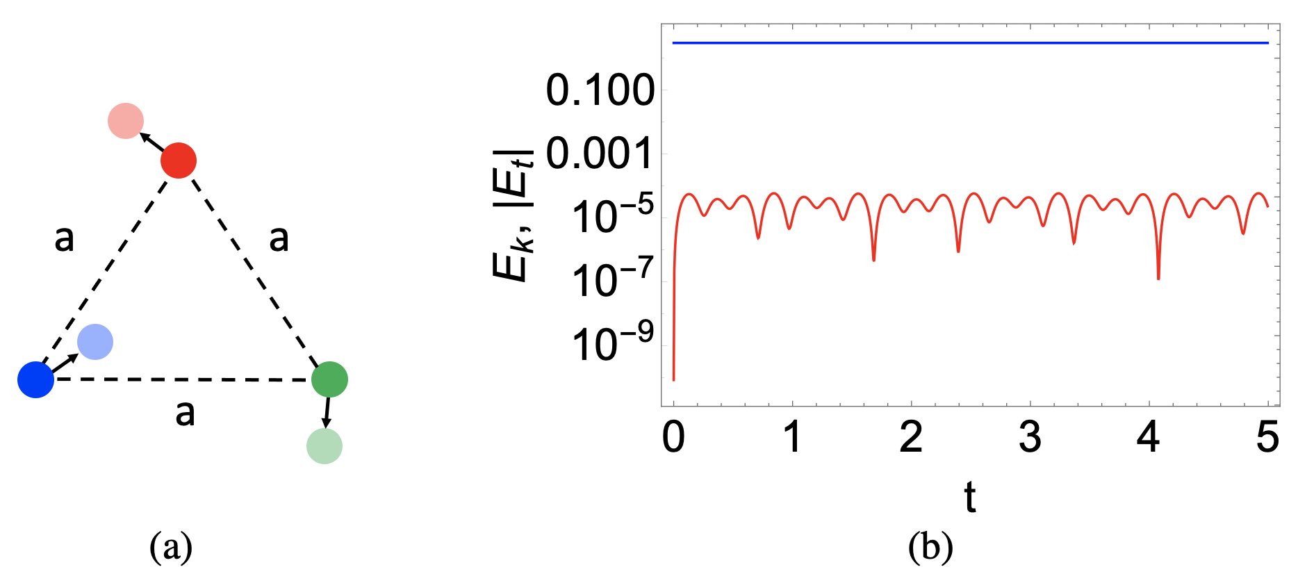
Figure 1: Typical energy variation in the perturbed three-body system under the Lennard-Jones potential. (a) Schematic plot of the disturbed triangular configuration of the triplet of particles in the plane. $a$ is the balance distance of the L-J potential. (b) Temporally varying kinetic energy (lower red curve) and the constant total energy (upper blue line). The disturbance amplitude $b=0.001$.

The microscopic dynamics of the particles upon disturbance is governed by the law of classical mechanics. The state of the system is characterized by the 6-dimensional vectors $\vec{X}$ and $\vec{V}$. $\vec{X}=\{r_{i\mu}\}$, and $\vec{V}=\{\dot{r}_{i\mu}\}$, where $r_{i\mu}$ is the $\mu$-component of the displacement of particle $i$. $i=1,2,3$. $\mu=x,y$. Specifically, $\vec{X}=(r_{1x},r_{1y},r_{2x},r_{2y},r_{3x},r_{3y})$. The sequence of the components is the same for $\vec{V}$. The equations of motion are cast as a pair of first-order differential equations:

$$\frac{d\vec{X}(t)}{dt} = \vec{V}(t),$$

$$\frac{d\vec{V}(t)}{dt} = \vec{f}(\vec{X}).$$ (2)

$\vec{f}(\vec{X})$ is a 6-dimensional vector whose component $f_{i\mu}$ gives the force on the particle $i$ in the $\mu$-direction; note that $i=1,2,3$, and $\mu=x,y$. The sequence of the components of $\vec{f}$ is consistent with both $\vec{X}$ and $\vec{V}$. The dependence of $\vec{f}$ on the displacement vector $\vec{X}$ is complicated due to the highly correlated particle motions. By linearization at the vertices of the equilibrium configuration, the expression for $\vec{f}(\vec{X})$ as a linear function of $\vec{X}$ could be written formally as:

$$f_{\alpha}(\vec{X})=-\beta_{0}K_{\alpha\beta}X_{\beta},$$ (3)

where $\beta_{0}=V_{LJ}^{\prime\prime}(a)$, and the $6\times 6$ matrix $K$ contains the cofficients of the linear terms. The matrix $K$, which is called the dynamical matrix, governs the dynamical evolution of the perturbed system in the linear regime. To explore the nonlinear regime, we numerically integrate Eqs.(2) using the standard Verlet method at high precision and obtain accurate trajectories of motion up to a hundred million time steps with well conserved energy, momentum and angular momentum Rapaport (2004); sup . Note that the algorithm of Verlet integration preserves the symplectic form on phase space that guarantees conservation of energy and momenta in long-time simulations. The typical time step is of order of $10^{-4}\tau_{0}$ by striking a balance on the conservation of relevant physical quantities and the efficiency of computation.

III Results and discussion

III.1 Dynamical analysis

We first slightly disturb the system, and analyze the temporal variation of the kinetic energy in order to extract key dynamical information Yao (2021). The variation of the kinetic energy in time is shown in Fig. 1(b). For reference, the constancy of the total energy is also shown by the horizontal blue line in Fig. 1(b). The associated single particle trajectories during the time intervals of $t\in[0,1.5]$ and $t\in[0,5]$ are shown in the lower panel in Fig. 2(a), where the red dot represents the initial position of the particle. The evolving particle trajectory weaves a highly regular parallelogrammic net bounded by four envelope lines. Longer time trajectories are presented in SI sup .

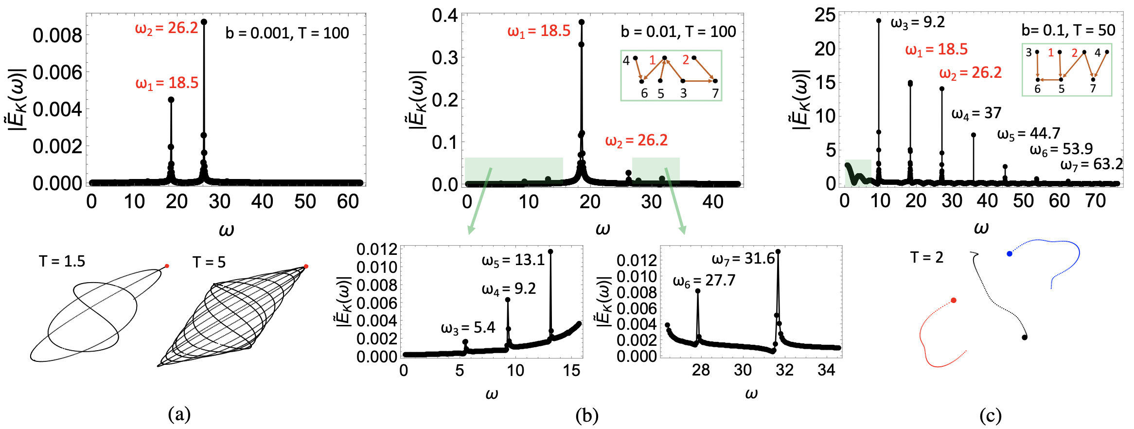
Figure 2: Frequency spectral analysis reveals nonlinear frequency-mixing processes in the disturbed three-body system. The frequency spectra of kinetic energy are obtained by discrete Fourier transformation. (a)-(c) The disturbance amplitude $b$ increases from $0.001$ to $0.1$. The relation of the emergent frequencies $\omega_{i}$ is presented in the inset graphs [see the green boxes in (b) and (c)]. The data are recorded in the sampling interval of $t\in[0,T]$. Associated particle trajectories during the time intervals of $t\in[0,T]$ for the linear and nonlinear cases are presented in the lower panels in (a) and (c).

To uncover the beat in the particle oscillations, we perform discrete Fourier transformation on the collected energy data Sundararajan (2001). A pair of fundamental modes are revealed as shown in Fig. 2(a). $\tilde{E}_{K}(\omega)$ is the Fourier transform of the time series of $E_{k}(t)$, where $t\in[0,T]$. The values of the fundamental frequencies are $\omega_{1}=18.5$, and $\omega_{2}=26.2$. The Lissajous-figure-like trajectory pattern in the lower panel of Fig. 2(a) results from a superposition of these two modes. Simulations also show that the basic peak structure in the $\tilde{E}_{K}(\omega)$-curve is invariant with the variation of the orientation of the initial displacement; the peaks become sharpened with the increase of the sampling interval $T$ sup .

To explore the physical origin of the pair of the fundamental modes, we analytically analyze the linearized equations of motion. Specifically, we analytically derive all of the matrix elements of the dynamical matrix $K_{\alpha\beta}$ sup , and obtain the nonzero eigenvalues: $\lambda_{1}=3/2$ and $\lambda_{2}=3$. Note that the first eigenvalue possesses the two-fold degeneracy. Each eigenvalue $\lambda$ corresponds to a normal mode of frequency $\omega_{\lambda}=\sqrt{\beta_{0}\lambda/m}$. Note that these fundamental frequencies derived in the linear regime are identical to those for the harmonic three-body system Saporta Katz and Efrati (2019); Saporta Katz and Efrati (2020). The associated frequency in the kinetic energy curve $E_{K}(t)$ is doubled:

$$\omega_{1} = 2^{\frac{11}{6}}3^{\frac{3}{2}}\approx 18.5,$$

$$\omega_{2} = \sqrt{2}\omega_{1}\approx 26.2.$$ (4)

These analytically derived frequencies are exactly those of the numerically solved fundamental modes in Fig. 2(a).

Here, we emphasize that the ratio of $\omega_{1}/\omega_{2}$ is an invariant for generic confining potentials; it is independent of particle mass and potential stiffness in equilibrium configuration. Furthermore, the two frequencies satisfy the non-resonance condition, suggesting the existence of dynamical complexity in the seemingly simple system Zaslavsky (2007). To substantiate this point, we record the crossing points of the evolving trajectory in Fig. 2(a) with some reference line up to $T=50$ following the spirit of Poincaré map, and numerically observe the filling of space in time by the aperiodic trajectory sup ; Kadanoff (1999); Altmann et al. (2006); Scheck (2010); Krylov (2014).

Upon stronger disturbance, richer frequency spectra are observed as presented in Figs. 2(b) and 2(c) for $b=0.01$ and $b=0.1$, respectively. As a characteristic of nonlinearity, we observe the proliferation of frequencies on the basis of the two fundamental frequencies $\omega_{1}$ and $\omega_{2}$ Fermi et al. (1955). By tracking the temporal variation of the peaks, we find that the dynamical state of the system is initially dominated by the single $\omega_{1}$ mode. The ensuing growth of the height of the peaks reflects the complicated partition of energy among the modes sup .

The connection of each emergent frequency and the two fundamental frequencies ($\omega_{1}$ and $\omega_{2}$) is illustrated in the inset graphs in Figs. 2(b) and 2(c). A vertex $i$ represents frequency $\omega_{i}$. The frequency at a vertex with a pair of incoming arrows is either the sum or the difference of the two frequencies at the ends of the arrows. Remarkably, a simple classical mechanical system consisting of only three particles is capable of supporting a series of complicated frequency-mixing processes, including the sum-frequency and difference-frequency generation. In Fig. 2(b), we further observe the fission of the fundamental mode $\omega_{1}$ into a pair of lower-frequency modes ($\omega_{1}\rightarrow\omega_{3}$ and $\omega_{5}$), and the frequency-halving process ($\omega_{1}\rightarrow\omega_{4}$, and $\omega_{2}\rightarrow\omega_{5}$) that is related to the bifurcation of orbits Scheck (2010). Similar frequency-halving phenomena have been reported in periodically poled active nonlinear crystals Chirkin et al. (2004).

Comparison of Figs. 2(b) and 2(c) shows the enhanced nonlinear effect as the disturbance amplitude $b$ is increased. Increasing $b$ leads to significant growth of the peak height and emergence of higher-frequency modes. Notably, secondary frequency-mixing events are observed in Fig. 2(c). For example, the combination of $\omega_{3}$ and $\omega_{5}$ leads to the new high-frequency $\omega_{6}$ mode. We also notice the accumulation of low-frequency modes to form a continuous frequency spectrum as indicated by the light green box in Fig. 2(c). Furthermore, the seemingly free motions of the particles, as plotted in the lower panel in Fig. 2(c), are highly correlated by the conservation of energy, momentum and angular momentum.

In preceding discussions, the particles interact by the L-J potential, which could be regarded as a nonlinear spring. To examine the generality of the key observations about the neat frequency-mixing events, we further study the triplet system connected by linear springs sup . In the perturbation regime, we observe a pair of fundamental modes that are identical to that in the L-J system as expected. At $b=0.1$ [corresponding to the case in Fig. 2(c)], we also observe the proliferation of new frequencies (but with much weaker strength as compared with the L-J system) and the featured frequency-mixing processes in the linear-spring system. The frequency spectra and relevant trajectories of the linear-spring system are presented in Supplemental Materials sup . These results indicate the existence of nonlinear dynamics even for a harmonic potential, implying the richness of the three-body system in dynamics.

It is known that the generation of new frequencies could be attributed to the nonlinear effect, which can be understood by analyzing the nonlinear equation of motion Landau and Lifshitz (1976) or by resorting to logistic mapping Feigenbaum (1978). In the specific three-body system under harmonic interaction, where the nonlinear effect as characterized by the proliferation of new frequencies also arises, the nonlinear interaction originates from the geometric configuration of the three particles, which is known as the geometric nonlinearity De Wijn and Fasolino (2009); Saporta Katz and Efrati (2019). The presence of a third particle brings in the nonlinear element that changes the original frequency structure of the original two-body system. Simulations show that the nonlinear effect vanishes by aligning the particles along a straight line. Thus, it shall be emphasized that the nonlinearity requires a non-zero balance length and placing the particles in a plane and not on a line. Here, we shall mention that the nonlinear dynamics of the harmonic three-body system has been discussed from the perspective of rotational random walk, where the spectral structure of the motion in terms of particle position (angular displacement or x coordinate) has been discussed, and the featured behavior of self-driven fractional rotational diffusion has been revealed Saporta Katz and Efrati (2019); Saporta Katz and Efrati (2020).

Regarding the free motions of the particles as constrained by the conservation laws in Fig. 2(c), it is of interest to mention that the conservation laws admit the counter-intuitive phenomenon of ejecting a particle to infinity in finite time in the Newtonian N-body system, as rigorously proved in mathematics Saari and Xia (1995). This phenomenon has motivated several deep mathematical conclusions related to the issue of singularity structure in classical mechanical systems.

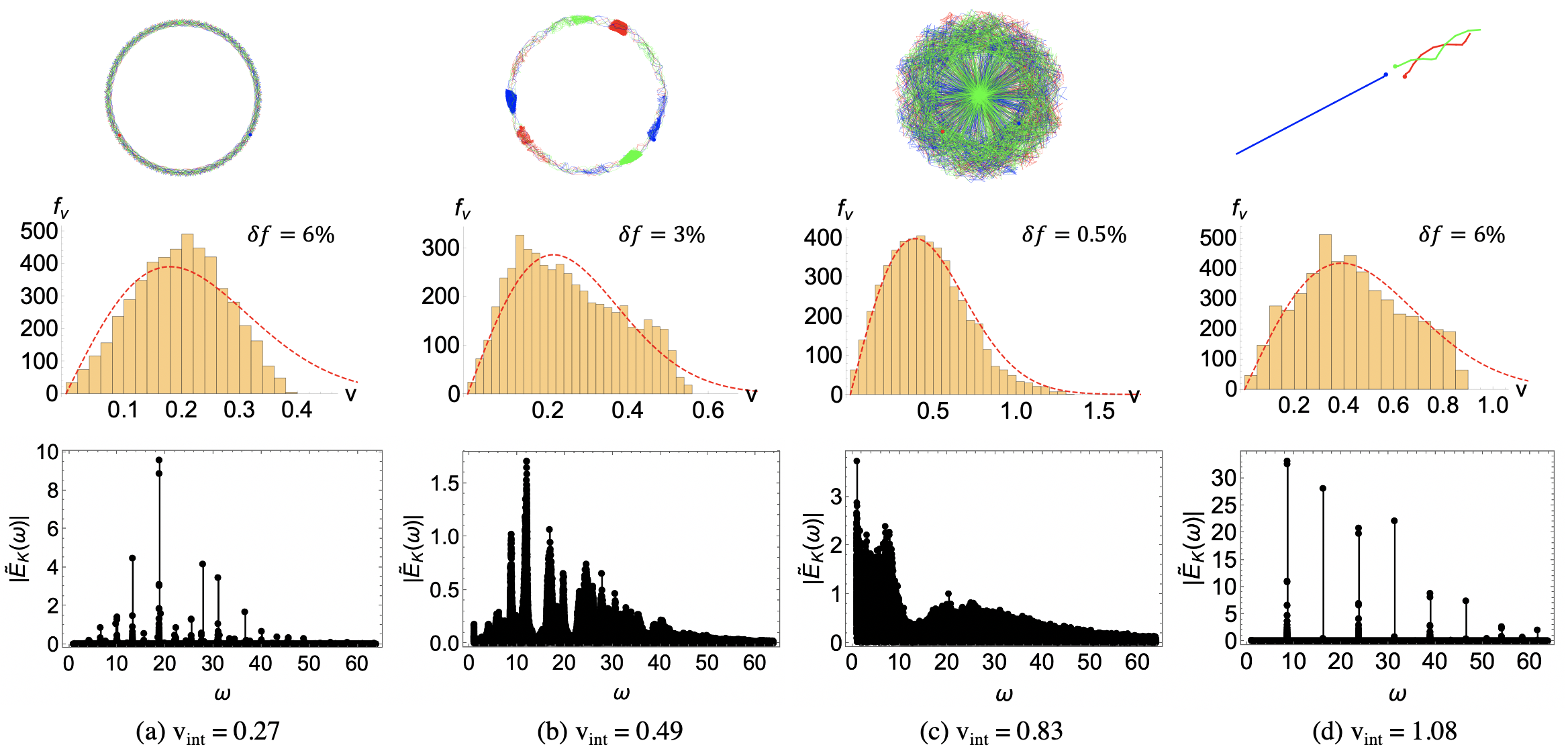
Figure 3: Statistical regularity arises in the classical three-body system under enhanced nonlinear effect. The histograms show the distribution of the instantaneous speed along a single particle trajectory at varying initial speed $v_{\textrm{ini}}$. For bounded motions in (a)-(c), the speed distribution approaches the Maxwell-Boltzmann distribution as $v_{\textrm{ini}}$ is increased. Note that this trend applies to all of the three particles. The fitting functions in the form of the Maxwell-Boltzmann distribution are plotted in dashed red curves. $\delta f$ is a measure of the deviation of the numerically obtained speed distribution from the Maxwell-Boltzmann distribution. Further increasing $v_{\textrm{ini}}$ leads to the free motion of the particles as shown in (d). The associated particle trajectories and the frequency spectra of kinetic energy are also presented; the three particles are distinguished by different colors. The particle speed is recorded at equal time interval $\Delta t=5$ up to $T=25000$.

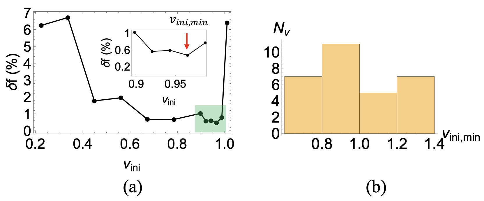
Figure 4: Statistical analysis on the convergence of the speed distribution to the two-dimensional Maxwell-Boltzmann distribution in the bounded motion under varying initial conditions. (a) A typical plot of $\delta f$ versus $v_{ini}$. $\delta f$ is the deviation between the numerically obtained speed distribution and the Maxwell-Boltzmann distribution. $v_{ini}$ is the magnitude of initial speed. The region in the green highlight is enlarged in the inset. $\delta f$ reaches minimum $\delta f_{min}$ when $v_{ini}=v_{ini,min}$. Dynamical transition from bounded to unbounded state occurs at the right end of the plot as $v_{ini}$ exceeds about $0.98$. (b) Histogram of $v_{ini,min}$ based on the data of particle speed under 30 independent initial conditions. $v_{ini,min}=0.97\pm 0.22$. The mean value of $\delta f_{min}$ is as small as $0.57\%$, indicating the good agreement between the numerical results and the Maxwell-Boltzmann distribution.

III.2 Statistical analysis

In the nonlinear regime, with the reduction of the regularity of motion due to the proliferation of frequencies, could any statistical regularity arise? In classical ideal gas, via frequent molecular collisions, the speed of the gas particles approaches the Maxwell-Boltzmann distribution as governed by the central limit theorem in the thermodynamic limit Maxwell (1860); Krylov (2014). Note that non-ergodic, stable motions of $N$ repulsive particles confined to a compact $d$-dimensional ($d\leq 2$) domain at sufficiently large energy is reported recently Rom-Kedar and Turaev (2022). Here, in the classical few-body system, could the nonlinearity effect fully randomize the particle speed to realize the distribution as in equilibrium systems of many particles?

To address this question, we work in the frame of reference where both the total momentum and angular momentum are zero. The initial condition is formulated by specifying the initial velocities of the three particles sup . Our statistical analysis is based on the single particle trajectory without resorting to the procedures of ensemble averaging and coarse-graining. We focus on the distribution of speed along a trajectory. In other words, the randomness of motion is discussed in the sense of speed distribution. The distributions of the speed data recorded at equal time interval are presented in Fig. 3. The associated trajectories of motion and the frequency spectra of kinetic energy are also shown in Fig. 3.

In the bounded motion of particles from Fig. 3(a) to 3(c), it is found that the speed distribution converges to the two-dimensional Maxwell-Boltzmann distribution, as indicated by the dashed red curve in Fig. 3(c). This trend applies to all of the three particles. To measure the deviation between the numerically obtained speed distribution and the Maxwell-Boltzmann distribution, we propose the quantity $\delta f$ as defined below:

$$\delta f=\frac{\sum_{v_{i}}(f(v_{i})-f_{M-B}(v_{i}))^{2}}{\sum_{v_{i}}f_{M-B}(v_{i})^{2}}.$$ (5)

$f(v)$ is the numerically obtained speed distribution, and $f_{M-B}(v)$ is the Maxwell-Boltzmann distribution.

$$f_{M-B}(v)\delta v=\Gamma v\exp(-v^{2}/2v_{p}^{2})\delta v,$$ (6)

where $v_{p}$ is the most probable speed. The values of $\delta f$ are given alongside the histograms in Fig. 3. The asymptotic process towards the speed distribution in Fig. 3(c) with the increase of the sampling interval $T$ is presented in SI sup . The value of $\delta f$ monotonously decreases from $20\%$ to $0.7\%$ when $T$ increases from $500$ to $10000$.

Simulations show that under varying initial conditions, the speed distribution uniformly converges to the two-dimensional Maxwell-Boltzmann distribution in the bounded motion with the increase of $v_{ini}$. Figure 4(a) shows a typical plot of $\delta f$ versus $v_{ini}$. We see that with the increase of $v_{ini}$, the value of $\delta f$ tends to decrease in the regime of bounded motion; dynamical transition from bounded to unbounded state occurs at the right end of the plot as $v_{ini}$ exceeds about $0.98$. The value of $\delta f$ reaches minimum when $v_{ini}=v_{ini,min}$, as indicated in the inset for the zoomed-in region in green highlight. For a collection of random orientations of the initial velocity, it is found that the value of $v_{ini}=v_{ini,min}$ is subject to a fluctuation: $v_{ini,min}=0.97\pm 0.22$, based on the data of particle speed under 30 independent initial conditions. The histogram of $v_{ini,min}$ is presented in Fig. 4(b). The mean value of $\delta f_{min}$ is as small as $0.57\%$, indicating the good agreement between the numerical results and the Maxwell-Boltzmann distribution.

Further increasing $v_{\textrm{ini}}$ leads to the dynamical transition from bounded to unbounded state. In the bounded motion, the region of motion evolves from an annulus [Fig. 3(a)] to a filled circle [Fig. 3(c)]. Notably, the trajectory in Fig. 3(b) shows simultaneous long-duration trapping of the triplet of particles within small angular intervals; quantitative analysis of this phenomenon is presented in SI sup . Such a L$\acute{e}$vy-flight-like phenomenon is related to the stickiness phenomenon of chaotic trajectories in the phase space of a Hamiltonian system Altmann et al. (2006); Zaslavsky (2007), and it has also been observed in the harmonic three-mass system Saporta Katz and Efrati (2019); Saporta Katz and Efrati (2020). The unbounded state in Fig. 3(d) is featured with the intertwined motion of the pair of particles and the ballistic motion of the remaining one. The associated frequency spectrum shows that such a dynamical state is dominated by a few discrete frequencies.

Comparison of the four cases in Fig. 3 shows that the Maxwell-Boltzmann distribution is reached when the trajectories of the three particles are fully mixed (see the upper insets), or when sufficiently large number of new frequencies are generated from the perspective of frequency spectra (see the lower insets). In other words, a great number of collisions among the particles are crucial for shaping the Maxwell-Boltzmann distribution along a single particle trajectory. Note that in the collisions of the particles, the large repulsive force between particles in short distance requires a sufficiently fine time step to reduce the particle displacement in a time step and to ensure the conservation of energy. Simulations show that the system energy is well conserved for the adopted time step at the order of $10^{-4}\tau_{0}$ sup . For the case that the speed of one particle is much larger than the remaining ones, as shown in Fig. 3(d), the fast particle may escape. Consequently, the trajectories could not be fully mixed, and the speed distribution is deviated from the Maxwell-Boltzmann distribution at least during the given simulation time. Note that even in this unbounded dynamical state, the nonlinear effect as characterized by the proliferation of frequencies is still present [see the lower panel in Fig. 3(d) for the spectral structure].

It shall be emphasized that the revealed statistical regularity in the speed distribution is neither resorting to any ensemble averaging nor by coarse-graining procedure. The element of randomness, which is crucial for shaping the regular statistical law in the few-body system, originates from the intrinsic dynamical nonlinearity without any external stimulus. Here, frequency spectrum analysis serves as a powerful tool to extract important nonlinear physics. Specifically, the nonlinearity caused frequency-mixing processes fully randomize the motion of the particles, and generate the regular distribution of instantaneous particle speed. We also note that the randomness of the motion is in the sense of the distribution of speed along a single trajectory, but not in the shape of the trajectory. This randomization mechanism is fundamentally different from the relaxation mechanism based on frequent molecular collisions in many-body systems Maxwell (1860); Cercignani et al. (1998). This finding may advance our understanding on the connection of classical dynamics and statistical mechanics. The foundation of statistical mechanics is usually assumed to be based on the presence of a large number of constituents and on ergodicity Kadanoff (1999); Scheck (2010); Krylov (2014), which has been challenged recently Gaveau and Schulman (2015). The present system consists of only three particles, and its dynamics is governed by the deterministic law. Yet, statistical regularity arises. Namely, the speed distribution along a single particle trajectory displays a good agreement with the regular Maxwell-Boltzmann distribution.

IV Conclusion

In summary, this work demonstrates how repeated application of simple laws leads to spatio-temporal complexity in a classical mechanical system consisting of only three particles. We have illustrated the elusive nonlinear dynamics and the connection of nonlinearity and random motion in terms of the neat frequency-mixing processes. We have also revealed the statistical regularity in particle speed underlying a single particle trajectory. The elucidation of the nonlinear dynamics and the emergent statistical regularity in this work may inspire further explorations into the fundamental questions on the interface of microscopic dynamics and statistical physics. Especially, the formally simple three-body system may serve as a suitable model to address these questions Saporta Katz and Efrati (2019); Saporta Katz and Efrati (2020). A possible extension of the current work is to endow the particles with distinct masses ($m_{i}$ for particle $i$), which brings in multiple time scales ($\tau_{i}=a\sqrt{m_{i}/\epsilon_{0}}$) and thus a wealth of dynamical behaviors arising from the interplay of these new time scales.

V ACKNOWLEDGMENTS

This work was supported by the National Natural Science Foundation of China (Grants No. BC4190050).

References

- Li and Yorke (1975) T.-Y. Li and J. A. Yorke, Am. Math. Mon. 82, 985 (1975).
- Cercignani et al. (1998) C. Cercignani et al., Ludwig Boltzmann: The Man Who Trusted Atoms (Oxford University Press, Oxford, 1998).
- Kadanoff (1999) L. P. Kadanoff, From Order to Chaos II (World Scientific, 1999).
- Dumas (2014) H. S. Dumas, The KAM Story (World Scientific Publishing Company, 2014).
- Krylov (2014) N. S. Krylov, Works On The Foundations of Statistical Physics (Princeton University Press, 2014).
- Neill et al. (2016) C. Neill, P. Roushan, M. Fang, Y. Chen, M. Kolodrubetz, Z. Chen, A. Megrant, R. Barends, B. Campbell, B. Chiaro, et al., Nat. Phys. 12, 1037 (2016).
- Sinai (1989) I. G. Sinai, Dynamical Systems II (Springer, 1989).
- Zwanzig (2001) R. Zwanzig, Nonequilibrium Statistical Mechanics (Oxford University Press, USA, 2001).
- Strogatz (2018) S. H. Strogatz, Nonlinear Dynamics and Chaos (CRC Press, 2018).
- Scheck (2010) F. Scheck, Mechanics: from Newton’s Laws to Deterministic Chaos (Springer Science & Business Media, 2010).
- Yang et al. (2017) B. Yang, J. Pérez-Ríos, and F. Robicheaux, Phys. Rev. Lett. 118, 154101 (2017).
- Tonks (1936) L. Tonks, Phys. Rev. 50, 955 (1936).
- Zheng et al. (1996) Z. Zheng, G. Hu, and J. Zhang, Phys. Rev. E 53, 3246 (1996).
- Cox and Ackland (2000) S. Cox and G. Ackland, Phys. Rev. Lett. 84, 2362 (2000).
- Cao et al. (2018) X. Cao, V. B. Bulchandani, and J. E. Moore, Phys. Rev. Lett. 120, 164101 (2018).
- Zaslavsky (2007) G. M. Zaslavsky, The Physics of Chaos in Hamiltonian Systems (World Scientific, 2007).
- Jones (1924) J. E. Jones, Proc. R. Soc. London, Ser. A. 106, 463 (1924).
- Yao (2017a) Z. Yao, Soft Matter 13, 5905 (2017a).
- Kob and Andersen (1995) W. Kob and H. C. Andersen, Phys. Rev. E 51, 4626 (1995).
- Xu et al. (2007) N. Xu, M. Wyart, A. J. Liu, and S. R. Nagel, Phys. Rev. Lett. 98, 175502 (2007).
- Rützel et al. (2003) S. Rützel, S. I. Lee, and A. Raman, Proc. R. Soc. London, Ser. A 459, 1925 (2003).
- Fukuda et al. (2017) H. Fukuda, T. Fujiwara, and H. Ozaki, J. Phys. A: Math. Theor. 50, 105202 (2017).
- Rahman (1964) A. Rahman, Phys. Rev. 136, A405 (1964).
- Tillack et al. (2016) A. F. Tillack, L. E. Johnson, B. E. Eichinger, and B. H. Robinson, J. Chem. Theory Comput. 12, 4362 (2016).
- Bienias et al. (2020) P. Bienias, M. J. Gullans, M. Kalinowski, A. N. Craddock, D. P. Ornelas-Huerta, S. L. Rolston, J. Porto, and A. V. Gorshkov, Phys. Rev. Lett. 125, 093601 (2020).
- Halperin and Nelson (1978) B. Halperin and D. R. Nelson, Phys. Rev. Lett. 41, 121 (1978).
- Strandburg (1988) K. J. Strandburg, Rev. Mod. Phys. 60, 161 (1988).
- Mitchell et al. (2017) N. P. Mitchell, V. Koning, V. Vitelli, and W. Irvine, Nat. Mater. 16, 89 (2017).
- Yao (2017b) Z. Yao, Phys. Rev. E 96, 062139 (2017b).
- Hwang et al. (2019) H. Hwang, D. A. Weitz, and F. Spaepen, Proc. Natl. Acad. Sci. U.S.A. 116, 1180 (2019).
- Vicsek and Zafeiris (2012) T. Vicsek and A. Zafeiris, Phys. Rep. 517, 71 (2012).
- Schaller and Bausch (2013) V. Schaller and A. R. Bausch, Proc. Natl. Acad. Sci. U.S.A. 110, 4488 (2013).
- Nguyen et al. (2014) N. H. Nguyen, D. Klotsa, M. Engel, and S. C. Glotzer, Phys. Rev. Lett. 112, 075701 (2014).
- Yao (2019) Z. Yao, Phys. Rev. Lett. 122, 228002 (2019).
- Fermi et al. (1955) E. Fermi, P. Pasta, S. Ulam, and M. Tsingou, Tech. Rep., Los Alamos Scientific Lab. (1955).
- Saporta Katz and Efrati (2019) O. Saporta Katz and E. Efrati, Phys. Rev. Lett. 122, 024102 (2019).
- Saporta Katz and Efrati (2020) O. Saporta Katz and E. Efrati, Phys. Rev. E 101, 032211 (2020).
- Maxwell (1860) J. C. Maxwell, Philos. Mag. 19, 19 (1860).
- (39) See Supplemental Material for technical details of the numerical approach, and supplemental information about trajectory evolution, frequency spectrum analysis of kinetic energy and statistical analysis of particle trajectories.
- Rapaport (2004) D. Rapaport, The Art of Molecular Dynamics Simulation (Cambridge University Press, Cambridge, UK, 2004).
- Yao (2021) Z. Yao, Europhys. Lett. 133, 54002 (2021).
- Sundararajan (2001) D. Sundararajan, The Discrete Fourier Transform: Theory, Algorithms and Applications (World Scientific, 2001).
- Altmann et al. (2006) E. G. Altmann, A. E. Motter, and H. Kantz, Phys. Rev. E 73, 026207 (2006).
- Chirkin et al. (2004) A. S. Chirkin, A. A. Novikov, and G. D. Laptev, J. Opt. B 6, S483 (2004).
- Landau and Lifshitz (1976) L. D. Landau and E. Lifshitz, Mechanics, 3rd Edition (Butterworth-Heinemann,Oxford, 1976).
- Feigenbaum (1978) M. Feigenbaum, J. Stat. Phys. 19(1), 25 (1978).
- De Wijn and Fasolino (2009) A. S. De Wijn and A. Fasolino, J. Phys. Condens. Matter 21, 264002 (2009).
- Saari and Xia (1995) D. G. Saari and Z. Xia, Notices of the AMS 42, 538–546 (1995).
- Rom-Kedar and Turaev (2022) V. Rom-Kedar and D. Turaev, arXiv:2208.14993 (2022).
- Gaveau and Schulman (2015) B. Gaveau and L. S. Schulman, Eur. Phys. J. Spec. Top. 224, 891 (2015).