LiteBIRD Science Goals and Forecasts: A full-sky measurement of gravitational lensing of the CMB

Abstract

We explore the capability of measuring lensing signals in LiteBIRD full-sky polarization maps. With a $30$ arcmin beam width and an impressively low polarization noise of $2.16\,\mu$K-arcmin, LiteBIRD will be able to measure the full-sky polarization of the cosmic microwave background (CMB) very precisely. This unique sensitivity also enables the reconstruction of a nearly full-sky lensing map using only polarization data, even considering its limited capability to capture small-scale CMB anisotropies. In this paper, we investigate the ability to construct a full-sky lensing measurement in the presence of Galactic foregrounds, finding that several possible biases from Galactic foregrounds should be negligible after component separation by harmonic-space internal linear combination. We find that the signal-to-noise ratio of the lensing is approximately $40$ using only polarization data measured over $90\%$ of the sky. This achievement is comparable to Planck’s recent lensing measurement with both temperature and polarization and represents a four-fold improvement over Planck’s polarization-only lensing measurement. The LiteBIRD lensing map will complement the Planck lensing map and provide several opportunities for cross-correlation science, especially in the northern hemisphere.

1 Introduction

Cosmic microwave background (CMB) polarization has been measured by multiple CMB experiments to improve constraints on cosmology. A CMB linear polarization map contains two spatial patterns: parity-even $E$-modes and parity-odd $B$-modes [1, 2]. In linear theory, density perturbations are the dominant source of the temperature anisotropies and $E$-mode polarization. The density perturbations do not produce the $B$-mode polarization without non-linear effects [3]. However, inflationary gravitational waves could generate the $B$-mode polarization [4, 5]. The main goal of the LiteBIRD experiment is the measurement of $B$-mode polarization produced by inflationary gravitational waves, which would be considered conclusive evidence for inflation in the early Universe [6].

Another effect that induces $B$-mode polarization is the weak gravitational lensing of the CMB. The mass distribution in the late Universe disturbs the trajectory of CMB photons, which distorts the spatial pattern of the observed polarization maps and converts part of the $E$-mode polarization into $B$-mode polarization [7]. The gravitational lensing distortion is a nonlinear effect on the CMB. A measurement of CMB lensing allows us to learn about the matter distribution in the late Universe. The lensing mass distribution correlates with tracers of the large-scale structure. Such correlations have been measured using, e.g., the galaxy number density [8, 9, 10, 11, 12, 13, 14, 15, 16, 17, 18, 19, 20, 21, 22, 23, 24, 25, 26, 27], cosmic shear [28, 29, 30, 31, 12, 32, 33, 34, 35, 36, 23, 37], the late-time integrated Sachs-Wolfe (ISW) effect in the CMB temperature fluctuations [38, 39, 40, 41], the thermal Sunyaev-Zel’dovich effect [42, 43], and the cosmic infrared background [44, 45, 46, 47, 48, 40, 49]. These cross-correlations have been used to constrain cosmology. In addition, the lensing map helps to improve the statistical uncertainty of the inflationary gravitational waves with so-called “delensing” [50, 51, 52].

The lensed CMB polarization data has off-diagonal correlations between angular multipoles, which can be utilized to reconstruct the gravitational lensing potential [53, 54]. Multiple CMB experiments have reconstructed the CMB lensing mass map. Its angular power spectrum has been measured, by the Atacama Cosmology Telescope [55, 56, 57, 58, 59, 60], BICEP [61, 62], Planck [63, 64, 40, 65], POLARBEAR [66, 67], and the South Pole Telescope [68, 69, 70, 71, 72]. Upcoming and future ground-based CMB experiments, including the Simons Observatory [73], CMB-S4 [74] and Ali CMB Polarization Telescope (AliCPT) [75], are planning to make high-sensitivity measurements of CMB polarization. Their target sensitivities are enough to measure the small-scale $B$-mode signal caused by lensing and significantly improve the precision of lensing measurements. After Planck  however, only LiteBIRD can reconstruct a full-sky lensing mass map including both the northern and southern hemispheres, which is impossible to achieve with a single ground-based experiment. Therefore, the LiteBIRD lensing mass map provides an exciting opportunity to cross-correlate the CMB lensing with galaxies on the sky. The LiteBIRD lensing map in the northern hemisphere would also be complementary with the AliCPT lensing map [75].

This work is part of a series of papers that present the science achievable by the LiteBIRD space mission, expanding on the overview of the mission published in Ref. [6] (hereafter, LB23). In particular, this work focuses on the initial investigation of the capability of measuring lensing signals with LiteBIRD. Multiple studies have explored the practical issues and developed mitigation techniques for these issues, such as survey boundary and source masking [76, 77, 78, 79, 80], inhomogeneous noise [78, 81], extragalactic foregrounds [79, 82, 83, 84, 85, 86, 87, 88, 89], and instrumental systematics on lensing measurements [90, 91]. Among practical concerns on lensing analysis, the Galactic foregrounds are one of the most important issues for LiteBIRD. Reference [92] shows that the residual Galactic foregrounds should be negligible in CMB-S4-like experiments that utilize small-scale CMB anisotropies. However, we use large-scale CMB polarization data in the LiteBIRD lensing measurement, where the Galactic foregrounds could be impactful [92]. This paper addresses this question by simulating the lensing reconstruction from a nearly full-sky LiteBIRD polarization map, including the component-separation procedure. We further investigate some applications of the LiteBIRD lensing map, including the primordial non-Gaussianity, the late-time ISW effect, and inflationary gravitational waves.

This paper is organized as follows. In Section  2, we explain our method for lensing reconstruction for LiteBIRD. In Sec. 3, we describe our setup for simulation. In Sec. 4, we show our main results for the lensing reconstruction for LiteBIRD. In Sec. 5, we investigate potential applications of the LiteBIRD lensing map for cosmology. Finally, Sec. 6 is devoted to a summary and discussion. Throughout this paper, we use the cosmological parameters for the flat $\Lambda$CDM model adopted in LB23. In a companion paper [93] (hereafter LB-Delensing), we explore the feasibility of delensing for LiteBIRD. We choose the cosmological parameters obtained from [94].

2 Methodology

This section describes our methodology for the lensing reconstruction from LiteBIRD polarization data. After briefly reviewing the principal impacts of weak gravitational lensing on CMB anisotropies, we summarize the quadratic estimator for the lensing reconstruction [54, 53], the internal-linear combination (ILC) in harmonic space (hereafter HILC) [95] for component separation, and filtering of the polarization map. The temperature map obtained from LiteBIRD will not offer significant improvement over the results already obtained by the Planck mission due to its restricted angular resolution. However, LiteBIRD will be able to precisely measure CMB polarization over the entire sky, providing a complementary full-sky lensing map that will have better accuracy at large angular scales ($L<10$) since the $EB$ quadratic estimator will be much less sensitive to several potential mean fields [79]. Our study focuses on the polarization measurements of LiteBIRD, where the polarization quadratic estimators yield the highest signal-to-noise ratio (SNR). The rest of this article will thus concentrate on polarization analysis.

2.1 Gravitational Lensing of CMB

The trajectories of CMB photons passing through a mass distribution are deflected by the gravitational potential which is referred to as gravitational lensing. The gravitational potential of the large-scale structure in the late-time Universe causes the gravitational lensing effect on the CMB, and the lensing effect distorts the observed CMB anisotropies. The lensed polarization anisotropies described by the Stokes $Q$ and $U$ parameters that we measure today are approximated as (e.g., Refs. [96, 97, 98])

$$\left[\tilde{Q}\pm i\tilde{U}\right](\hat{\bm{n}}) =\left[Q\pm iU\right](\hat{\bm{n}}+\bm{d})\,,$$ (2.1)

where $\hat{\bm{n}}$ is the line-of-sight unit vector and $\bm{d}$ is the deflection vector. We define the lensing potential, $\phi$, as $\bm{d}=\bm{\nabla}\phi$, where $\bm{\nabla}$ is the covariant derivative on the sphere. The lensing potential is related to the line-of-sight projection of the three-dimensional gravitational potential (the so-called Weyl potential [97]), $\Psi$, sourced by the matter distribution, as

$$\phi(\hat{\bm{n}})=-2\int_{0}^{\chi^{*}}d\chi\frac{\chi^{*}-\chi}{\chi^{*}\chi}\Psi(\chi\hat{\bm{n}},\eta_{0}-\chi)\,.$$ (2.2)

Here, $\chi$ is the conformal distance, $\eta_{0}$ is the conformal time today, and $\chi^{*}$ is the conformal distance to the last-scattering surface. The gravitational potential, $\Psi(\chi\hat{\bm{n}},\eta_{0}-\chi)$, is evaluated along the unperturbed trajectory $\chi\hat{\bm{n}}$, the so-called Born approximation [100, 101, 102], with conformal time $\eta_{0}-\chi$. We ignore the curl mode, which vanishes in the linear theory of perturbations having only scalar density perturbations (see, e.g., Ref. [103] and reference therein).

Furthermore, the lensing converts part of the $E$-mode polarization into $B$-mode polarization [104]. The lensing-induced $B$-mode polarization is roughly comparable to a $5\,\mu$K-arcmin white noise up to half-degree angular scale and has been detected by ground-based CMB experiments (e.g., Ref. [46]). This lensing $B$-mode polarization impedes the detection of inflationary gravitational waves [51]. LB-Delensing focuses on overcoming this issue with delensing techniques, which we will also mention in Sec. 5.

2.2 Reconstruction of Lensing Potential

The lensing potential can be reconstructed using the fact that averaging over CMB realizations, while keeping the lensing potential unchanged, violates the statistical isotropy of the CMB, thereby introducing correlations between different CMB polarization multipoles. The off-diagonal elements of the CMB polarization covariance generated by lensing up to linear order in $\phi$ are given as [53, 105]

$$\langle X_{\ell m}Y_{\ell^{\prime}m^{\prime}}\rangle_{(\ell m)\not=(\ell^{\prime},-m^{\prime})}=\sum_{LM}(-1)^{M}\left(\begin{array}[]{clcr}\ell&\ell^{\prime}&L\\ m&m^{\prime}&-M\end{array}\right)f^{XY}_{\ell\ell^{\prime}L}\phi_{LM}\,,$$ (2.3)

where $X$, $Y\in\{E,B\}$ and the quantity in parentheses is the Wigner 3$j$ symbol that represents the angular momentum coupling. The function $f^{XY}_{\ell\ell^{\prime}L}$ quantifies the response of the off-diagonal correlations to lensing whose explicit form is given by Table 1 in Ref. [53]. Thus, the lensing potential can be estimated as a quadratic combination of the CMB anisotropies at different angular scales.

In the LiteBIRD case, the $EB$ estimator dominates the SNR of lensing. The improvement of the SNR using the iterative estimator is negligible for the LiteBIRD case. Therefore, this paper only focuses on the $EB$ quadratic estimator. In an idealistic case, the estimator is given as [53]

$$\hat{\phi}_{LM}=A_{L}^{\phi}(\bar{\phi}_{LM}-\langle\bar{\phi}_{LM}\rangle)\,,$$ (2.4)

where we define

$$\bar{\phi}^{*}_{LM}=\sum_{\ell\ell^{\prime}}\begin{pmatrix}\ell&\ell^{\prime}&L\\ m&m^{\prime}&M\end{pmatrix}(f^{EB}_{\ell\ell^{\prime}L})^{*}\bar{E}_{\ell m}\bar{B}_{\ell^{\prime}m^{\prime}}\,.$$ (2.5)

In an idealistic case, the filtered multipoles, $\bar{E}_{\ell m}$ and $\bar{B}_{\ell m}$, are obtained by multiplying their inverse variance for each multipole, $\bar{X}_{\ell m}=X_{\ell m}/C^{XX}_{\ell}$, with $X=E$ or $B$. In this study, we employ Wiener filtering, including the pixel-space noise covariance, the details of which are described in Sec. 2.4. The normalization in the idealistic full-sky case is given by

$$A_{L}^{\phi}=\left\{\frac{1}{2L+1}\sum_{\ell\ell^{\prime}}\frac{|f^{EB}_{\ell\ell^{\prime}L}|^{2}}{C^{EE}_{\ell}C^{BB}_{\ell^{\prime}}}\right\}^{-1}\,.$$ (2.6)

In the following, we describe how to implement the estimator for LiteBIRD.

2.3 Galactic Foreground Cleaning

We perform lensing reconstruction on the foreground-cleaned polarization map. Our simulation includes both Galactic dust and synchrotron emission, with spatially varying spectral indices. Point sources and free-free emission are excluded, since their impact on large angular CMB multipoles is insignificant [108, 109]. The harmonic coefficients of our frequency maps at each observed frequency $\nu$ are modeled as

$$M_{\ell m}^{\nu}=S^{\rm CMB}_{\ell m}+S_{\ell m}^{{\rm FG},\nu}+N_{\ell m}^{\nu}\,,$$ (2.7)

where $S^{\rm CMB}_{\ell m}$ is the CMB component, $S_{\ell m}^{{\rm FG},\nu}$ is the total foreground contribution at the observing frequency $\nu$, and $N^{\nu}_{\ell m}$ is the noise at the frequency $\nu$. The assumption of a known frequency scaling permits the utilization of ILC in harmonic space for the cleaning. An additional critical assumption underlying the ILC method is the Gaussianity of the CMB. In HILC, we define the foreground-cleaned map as [95]

$$S^{\rm cleaned}_{\ell m}=\bm{w}_{\ell}\cdot\bm{M}_{\ell m}\,,$$ (2.8)

where $\bm{w}_{\ell}$ contains the weights for each frequency map, and the bold letters indicate the vectors containing all observed frequency maps. We can derive the HILC weights by minimizing the variance from the foregrounds and noise contributions under the constraint for an unbiased estimate, $\bm{w}_{\ell}^{\mathrm{T}}\cdot\bm{a}=1$, with $\bm{a}=(1,1,\dots,1)^{\mathrm{T}}$. The weights are then given by

$$\bm{w}_{\ell}=\frac{{\bm{\mathrm{C}}}_{\ell}^{-1}\bm{a}}{\bm{a}^{\mathrm{T}}{\bm{\mathrm{C}}}_{\ell}^{-1}\bm{a}}\,,$$ (2.9)

where the covariance of frequency maps in harmonic space is given by

$${\bm{\mathrm{C}}}_{\ell}=\frac{1}{2\ell+1}\sum_{m}\bm{M}_{\ell m}\bm{M}_{\ell m}^{\dagger}\,.$$ (2.10)

The HILC method requires the total power spectrum, which includes contributions from the CMB, Galactic foregrounds, and noise, to compute the covariance of the frequency maps. In practice, this total power spectrum is estimated from observed data. On the other hand, the method does not include the non-Gaussianity of the Galactic foregrounds. Unlike other component-separation methods, the HILC method focuses on minimizing the variance in the foreground cleaned map while preserving the signal power, rather than globally suppressing the statistical noise. HILC assumes isotropy to derive the weights, in contrast to, for example, Needlet ILC [110]. This isotropic assumption limits the ability of HILC to optimally account for spatial variations in foreground morphology and spectral energy distribution (SED), potentially introducing bias in the lensing measurements due to the spatial variation of Galactic foregrounds. This paper tests whether the HILC method works even if the Galactic foregrounds have some spatial variation.

2.4 Filtering of CMB anisotropies

We compute the Wiener-filtered $E$- and $B$-mode polarization starting from the above component-separated polarization map as inputs. Specifically, we solve the following equation [111, 112]:

$$\left[1+{\bm{\mathrm{C}}}_{\rm s}^{1/2}{\bm{\mathrm{B}}}{\bm{\mathrm{Y}}}_{2}^{\dagger}{\bm{\mathrm{N}}}_{\rm pix}^{-1}{\bm{\mathrm{Y}}}_{2}{\bm{\mathrm{B}}}{\bm{\mathrm{C}}}_{\rm s}^{1/2}\right]({\bm{\mathrm{C}}}_{\rm s}^{-1/2}\bm{\widehat{p}}^{\rm WF})={\bm{\mathrm{C}}}^{1/2}_{\rm s}{\bm{\mathrm{B}}}{\bm{\mathrm{Y}}}^{\dagger}_{2}{\bm{\mathrm{N}}}_{\rm pix}^{-1}\bm{\widehat{p}}^{\rm obs}\,.$$ (2.11)

Here, we solve for the vector $\bm{\widehat{p}}^{\rm WF}$, which has the harmonic coefficients of the Wiener-filtered $E$- and $B$-mode polarization, ${\bm{\mathrm{C}}}_{\rm s}$ is the diagonal signal covariance of the lensed $E$- and $B$-mode polarization in spherical-harmonic space, and ${\bm{\mathrm{B}}}$ is a diagonal matrix to include the beam smearing. The matrix ${\bm{\mathrm{C}}}_{\rm s}^{1/2}$ is defined so that its square is equal to ${\bm{\mathrm{C}}}_{\rm s}$. The real-space vector $\bm{\widehat{p}}^{\rm obs}$ contains the observed Stokes $Q$ and $U$ maps after adopting HILC. The matrix ${\bm{\mathrm{Y}}}_{2}$ is defined to transform the multipoles of the $E$- and $B$-modes into real-space maps of the Stokes parameters $Q$ and $U$. Finally, ${\bm{\mathrm{N}}}_{\rm pix}$ is the pixel-space covariance matrix of the instrumental noise in these maps.

To compute the noise covariance, we assign infinite noise for pixels not used in the analysis. We assume isotropic noise in observed pixels, following a model of $E$- and $B$-mode noise power spectra. Explicitly, we assume that the inverse noise covariance is given by

$${\bm{\mathrm{N}}}_{\rm pix}^{-1}={\bm{\mathrm{W}}}{\bm{\mathrm{Y}}}_{2}{\bm{\mathrm{N}}}^{-1}{\bm{\mathrm{Y}}}^{\dagger}_{2}{\bm{\mathrm{W}}}\,,$$ (2.12)

where ${\bm{\mathrm{W}}}$ is a matrix that takes the value 1 for pixels used in the analysis and zeroes otherwise, and ${\bm{\mathrm{N}}}$ is the noise covariance of $E$ and $B$ modes. We assume that the noise covariance of $E$- and $B$- modes is diagonal in harmonic space, with elements given by a model of the $E$- and $B$- mode noise power spectra, $N^{EE}_{\ell}$ and $N_{\ell}^{BB}$. Our simulation pipeline uses the noise spectra obtained from the HILC weights during component separation with the reference noise spectra of $15$ frequency channels. We do not include any extra masks besides the Galactic mask.

3 Simulations

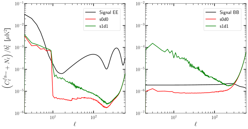
Figure 1: Foreground residuals and noise presented in our component-separated polarization maps. The solid black line represents the signal. The left and right panels display the $E$- and $B$-mode residuals, respectively. We illustrate the residuals for two foreground models, s0d0 (red) and s1d1 (green). Note that the green curves deviate significantly from the assumed model during component separation, substantially increasing residuals. Both spectra are computed from $500$ full-sky simulations.

This section overviews the simulation sets used in this analysis and in LB-Delensing to produce the results. We use the experimental specifications described in table $13$ of LB23 to generate multiple frequency maps with frequency coverage ranging from $40\,$GHz to $402\,$GHz in $15$ frequency channels. Note that while table $13$ of LB23 provides $22$ frequency channels, we exclusively consider the combined values for each frequency. However, our investigation finds that the changes in the noise properties remain negligible in the foreground-cleaned map, even when utilizing the full $22$-frequency configuration.

We generate realizations of the frequency maps and the post-component-separation map through the following steps.

1. We create a lensed CMB polarization map of the full sky. We first generate unlensed CMB polarization maps and a lensing potential map on the full sky as random Gaussian fields drawn from the input fiducial angular power spectra. We then remap the unlensed CMB maps with the lensing potential map using lenspyx, where the algorithm utilizes bicubic interpolation in an oversampled equidistant-cylindrical-projection grid.

2. We produce $15$ frequency maps of synchrotron and dust emission using pysm3. For our baseline simulation set we use s1 and d1 models for synchrotron and dust, respectively. In the s1 model, a power law scaling is applied to the synchrotron emission templates [113, 114] with a spatially varying spectral index [115]. The thermal dust, d1, is modeled as a single-component modified blackbody. The Planck dust template is scaled to different frequencies with a modified-blackbody spectrum using spatially varying temperature and spectral index [116]. In our analysis, we also consider the d0 model for dust and the s0 model for synchrotron radiation, both sourced from PySM. Here, the d0 model corresponds to a simplified version of the d1 model, characterized by a fixed spectral index of $1.54$ and a blackbody temperature of $20\,$K. On the other hand, the s0 has a constant spectral index of $-3$.

3. Each frequency map containing the CMB signal and the foreground components is convolved with the associated Gaussian beam, and then the corresponding white noise is added to each frequency map.

4. We deconvolve the aforementioned beam-convolved frequency maps and perform component separation using the HILC algorithm with fgbuster to obtain the full-sky component-separated map. HILC uses an evenly binned covariance, with bin size, $\Delta\ell=10$.

We repeat this process for each realization and generate $500$ realizations (hereafter SET1). These maps are defined on a Healpix [117] grid with $N_{\rm side}=512$. In addition, we generate a simulation set to specifically compute the so-called $N^{(1)}$ bias in the lensing measurement [118], where the input lensing map is kept fixed for all realizations. This fixed-lensing simulation is generated for $100$ realizations (hereafter SET2).

Figure 1 shows the $E$- and $B$-mode angular power spectra of the component-separated CMB maps on the full sky. At large angular scales ($\ell\lesssim 100$), the residual foregrounds become non-negligible, especially for the $B$-mode power spectrum, which is dominated by residual foregrounds at $\ell\lesssim 100$. At smaller angular scales ($\ell\gtrsim 600$), the instrumental noise becomes dominant.

4 Lensing Reconstruction

In this section, we present the results of the reconstruction of lensing potential from our simulation set. For the forecast, we consider the s1d1 foreground model as our baseline simulation. We also highlight the biases in our estimates of the lensing power spectrum.

4.1 Reconstructed Lensing Map

We reconstruct the lensing potential from the component-separated maps using the public Planck Galactic mask that keeps $80\%$ of the sky. Before this reconstruction, we apply the filtering as described in Eq. (2.11) of Sec. 2.4 to the component-separated maps. The HILC-weighted noise spectra averaged over the SET1 simulation are used for the noise covariance, ${\bm{\mathrm{N}}}$. We employed the $EB$ quadratic estimator with cmblensplus [119] for reconstructing the lensing deflection field. For the analysis of this paper, CMB multipoles $2<\ell<600$ were used. The maximum multipole is determined so that the SNR of the lensing signals is saturated.

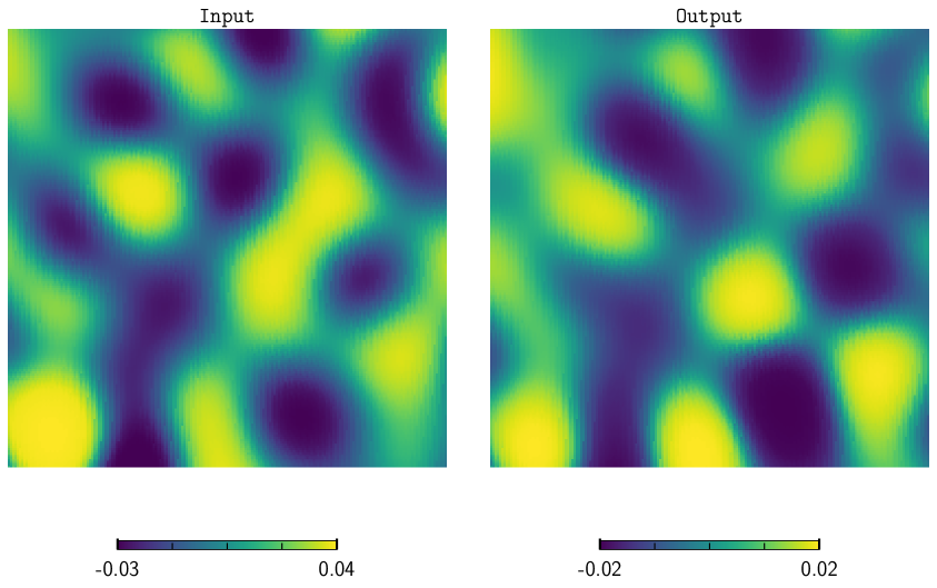
Figure 2: Lensing convergence map, which is defined in harmonic space as $\kappa_{LM}\equiv L(L+1)\phi_{LM}/2$ in harmonic space, obtained from one realization of the SET1 s1d1 simulation. The map contains multipole of $2<L<100$. Left: The input map used to remap the primary CMB. Right: The Wiener-filtered reconstructed map. The map resolution is $5$ arcmin-pixel^-1.

Figure 2 shows one realization of the reconstructed lensing-convergence map. We can see a clear correlation between the input and reconstructed lensing maps.

4.2 Biases in the Lensing Power Spectrum Estimate

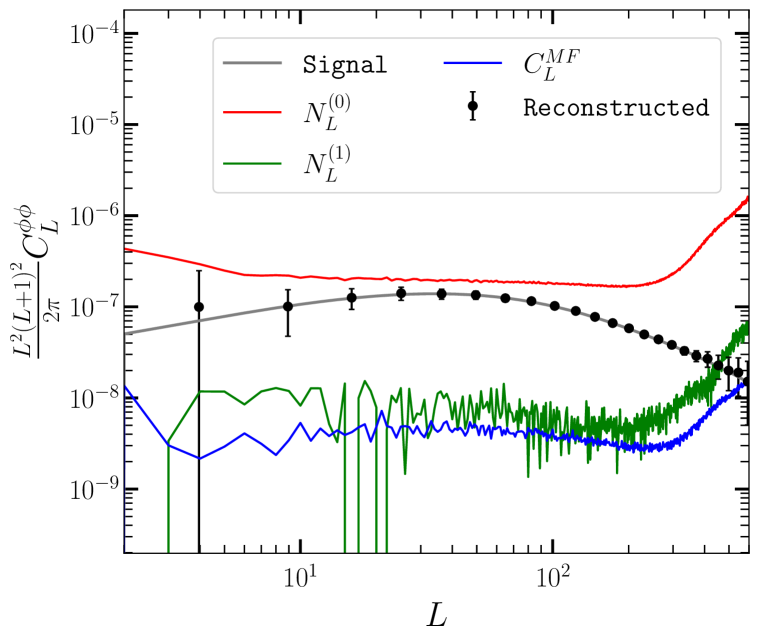
Figure 3: Binned angular power spectrum of the lensing potential shown in the black with error bars. The mean and standard deviation are obtained from $400$ realizations of the SET1 simulation. The red and green solid lines are the MCN0 and MCN1 biases, respectively. The mean field is shown with a blue line. We use the s1d1 model for this analysis. We show the power spectrum up to $L=600$ since the power spectrum at $L>600$ is significantly noise-dominant.

The estimation of the angular power spectrum of the lensing potential requires the subtraction of several biases because the estimates of the lensing potential are quadratic in CMB polarization anisotropies, and the power spectrum of the lensing estimator is the four-point correlation of the CMB anisotropies. The CMB four-point correlation consists of contributions from disconnected and connected parts, and the latter contains the lensing potential power spectrum. The remaining terms emerge as a bias in estimating the lensing power spectrum [118, 120, 121, 122]. The power spectrum of the quadratic estimator, $C_{L}^{\hat{\phi}\hat{\phi}}$, is described by

$$C_{L}^{\hat{\phi}\hat{\phi}}=R_{L}C_{L}^{\phi\phi}+N_{L}^{(0)}+N_{L}^{(1)}+\Delta C^{\phi\phi}_{L}\,.$$ (4.1)

The first term is the lensing potential power spectrum, $C_{L}^{\phi\phi}$, multiplied by a factor, $R_{L}$, due to a mismatch between the analytic and true normalizations. The second term, $N_{L}^{(0)}$, arises from the disconnected part of the four-point correlation, the so-called $N0$ bias, which receives contributions from the CMB, foreground, and noise. The third term, $N_{L}^{(1)}$, is the so-called $N1$ bias that arises from the secondary contraction of the connected parts by lensing at first order in $C_{L}^{\phi\phi}$ [118], and the last term, $\Delta C^{\phi\phi}_{L}$, contains the other remaining biases of $C^{\phi\phi}_{L}$ due to, e.g., possible issues of the estimation of normalization, mixing of power between different multipoles, and biases at ${\cal O}((C_{L}^{\phi\phi})^{2})$.

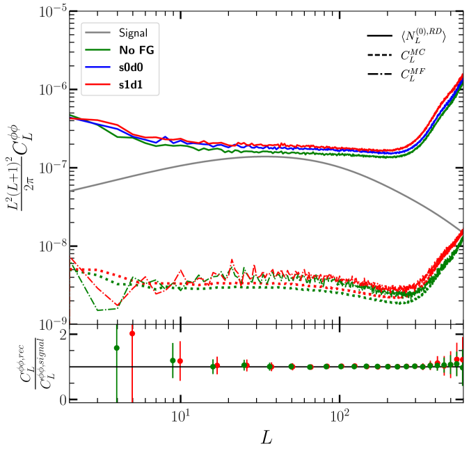
Figure 4: Top: Comparison plot of the N0 (upper, colored solid) and mean-field biases (lower, colored dash-dotted), with and without the Galactic foregrounds. For the N0 bias, we show two foreground cases, s0d0 and s1d1, in addition to the no foreground case (‘No FG’). We also show the Monte Carlo error in estimating the mean-field bias, $C_{L}^{\rm MC}$, (dotted), and the lensing power spectrum signal (gray solid). Bottom: The ratio of the measured lensing power spectrum to the input lensing power spectrum with (red) and without (green) the Galactic foregrounds. Note that the power spectrum shown in red is shifted to the right as $L\to L+1$ for clarity.

We estimate the mean-field bias, $\langle\hat{\phi}_{LM}\rangle$, which arises primarily due to the mask and foreground residuals, using $100$ realizations of the SET1 simulation. The mean-field bias is subtracted at the map level as shown in Eq. (2.4), and these realizations are not included in computing other bias terms. To check the level of the mean-field bias, we also compute the power spectrum of the mean-field bias, $C_{L}^{\rm MF}$.

The $N0$ bias approximately corresponds to the noise power spectrum of the reconstructed lensing map. We compute the $N0$ bias with a Monte Carlo simulation (hereafter MCN0). Specifically, we compute the lensing estimator using the SET1 simulation in the following way:

$$N_{L}^{(0),\rm MC}\equiv\Big{\langle}C_{L}^{\hat{\phi}\hat{\phi}}\left[E^{i},B^{j},E^{i},B^{j}\right]+C_{L}^{\hat{\phi}\hat{\phi}}\left[E^{i},B^{j},E^{j},B^{i}\right]\Big{\rangle}_{\rm SET1}\,,$$ (4.2)

where $i$ and $j$ are simulation indices, and we define

$$C_{L}^{\hat{\phi}\hat{\phi}}\left[X,Y,X^{\prime},Y^{\prime}\right]\equiv C_{L}^{\hat{\phi}^{XY}\hat{\phi}^{X^{\prime}Y^{\prime}}}\,.$$ (4.3)

The ensemble average is over $500$ realizations from SET1 with $i$ and $j=i+1$ changing cyclically. Since the MCN0 estimate is not optimal [123, 124], we also compute the realization-dependent $N0$ (hereafter RDN0) bias [79, 64] for each realization in SET2, which is given by

$$\begin{split}N_{L,i}^{(0),\rm RD}&\equiv\langle C_{L}^{\hat{\phi}\hat{\phi}}\left[E^{i},B^{j},E^{i},B^{j}\right]+C_{L}^{\hat{\phi}\hat{\phi}}\left[E^{j},B^{i},E^{i},B^{j}\right]\\ &\quad+C_{L}^{\hat{\phi}\hat{\phi}}\left[E^{i},B^{j},E^{j},B^{i}\right]+C_{L}^{\hat{\phi}\hat{\phi}}\left[E^{j},B^{i},E^{j},B^{i}\right]\rangle_{j}\\ &\quad-N_{L}^{(0),\rm MC}\,.\end{split}$$ (4.4)

The average is over $100$ realizations with $j=i+1$, which is independent of that used for evaluating $N_{L}^{(0),\rm MC}$. The $N1$ bias is estimated with the SET2 simulation as (e.g., Ref. [69], hereafter MCN1)

$$N_{L}^{(1),\rm MC}\equiv\left\langle C_{L}^{\hat{\phi}\hat{\phi}}\left[E^{i},B^{j},E^{i},B^{j}\right]+C_{L}^{\hat{\phi}\hat{\phi}}\left[E^{i},B^{j},E^{j},B^{i}\right]\right\rangle_{\text{SET2}}-N_{L}^{(0),\rm MC}\,.$$ (4.5)

Here, we use $100$ realizations of the SET2 simulations to evaluate the ensemble average.

Figure 3 shows the significance of each bias term compared with the input theoretical lensing power spectrum. We also show the debiased angular power spectrum of lensing potential:

$$\hat{C}_{L}^{\phi\phi}=\frac{1}{R^{\rm MC}_{L}}\left(C_{L}^{\hat{\phi}\hat{\phi}}-N_{L}^{(0),\rm RD}-N_{L}^{(1),\rm MC}\right)\,,$$ (4.6)

where $R^{\rm MC}_{L}$ is the normalization correction obtained from

$$R^{\rm MC}_{L}=\left(\frac{C_{L}^{\phi^{\rm in}\hat{\phi}}}{C_{L}^{\phi^{\rm in}\phi^{\rm in}}}\right)^{2}\,.$$ (4.7)

Here, $\phi^{\rm in}$ is the full sky input lensing map. We use $400$ realizations of the SET1 simulations to obtain the mean and standard deviation of $\hat{C}_{L}^{\phi\phi}$. After correcting for the N0 bias, N1 bias, and normalization, the power spectrum is in good agreement with the input power spectrum. This indicates that $\Delta C^{\phi\phi}_{L}$ is negligible. The result also shows that the foreground-induced trispectrum and mean-field bias are negligible.

In Figure 4, we compare the $N0$ and mean field biases of the lensing reconstruction in the presence and absence of Galactic foregrounds. Without Galactic foregrounds, the only non-idealistic effect is the Galactic mask, which primarily causes the mean-field bias. With the foreground cleaning, the noise level of the cleaned CMB polarization map increases, leading to an increase in the $N0$ bias. The power spectrum of the mean-field bias is more than an order of magnitude lower than the signal power spectrum. The mean field does not increase even in the presence of the residual Galactic foregrounds.

4.3 The signal-to-noise ratio

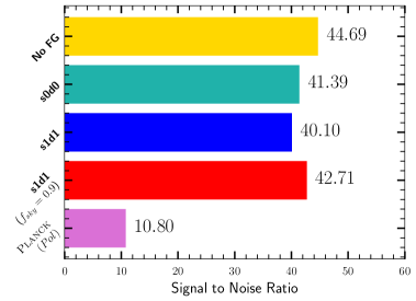
Figure 5: SNR of the lensing power spectrum. The yellow bar shows the case with no foregrounds, while the light green and blue bars represent the cases with the s0d0 and s1d1 foreground models, respectively. The red bar shows the case with the s1d1 foreground model but with a wider sky coverage, $f_{\rm sky}=0.9$. The pink bar is the SNR from the Planck polarization-based lensing analysis [65].

We here show a simulation-based estimate of the SNR of the lensing signal. We first measure the amplitude of the lensing spectrum from a weighted mean over multipole bins:

$$\hat{A}_{\rm lens}=\frac{\sum_{b}a_{b}\hat{A}_{b}}{\sum_{b}a_{b}}\,.$$ (4.8)

The quantity $\hat{A}_{b}$ is the relative amplitude of the power spectrum compared with a fiducial power spectrum for the Planck $\Lambda$CDM cosmology, $C_{b}^{\phi\phi}$, i.e., $\hat{A}_{b}\equiv\hat{C}_{b}^{\phi\phi}/C_{b}^{\phi\phi}$. The weights, $a_{b}$, are taken from the band-power covariance as

$$a_{b}=\sum_{b^{\prime}}C^{\phi\phi}_{b}{\bm{\mathrm{Cov}}}_{bb^{\prime}}^{-1}C^{\phi\phi}_{b^{\prime}}\,.$$ (4.9)

The fiducial band-power values and their covariances, including off-diagonal correlations between different multipole bins, are evaluated from the simulations. The SNR is then given by

$${\rm SNR}=\frac{1}{\sigma_{A}}\,,$$ (4.10)

where $\sigma_{A}$ is the $1\,\sigma$ constraint on $A_{\rm lens}$ computed from SET1 simulations.

Figure 5 shows a summary of the SNR for three cases: the baseline, s0d0, and no-foreground cases. We find that the SNR of the LiteBIRD lensing reconstruction is comparable to that of the latest full-sky lensing measurement from Planck [40]. In the presence of the s0d0 foregrounds, the SNR decreases by $10$% compared to the no-foreground case. If we consider the foregrounds with the spatially varying spectral index, the SNR decreases by $3$% compared to the s0d0 case. It is worth noting that LiteBIRD uses polarization alone, and the reconstructed map from LiteBIRD is complementary to the Planck lensing map, which is mostly based on temperature anisotropies. If we increase the sky fraction to $f_{\text{sky}}=0.9$, the SNR increases by $6.8$%, a factor of 4 improvement compared to the Planck polarization-only reconstruction (referred to as Pol hereafter).

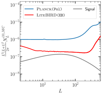
Figure 6: Comparison of $N_{L}^{(0),{\rm MC}}$ between Planck and LiteBIRD. The gray solid line represents the signal, while the blue and red solid lines correspond to the noise bias in the Planck and LiteBIRD polarization-based estimates, respectively.

Figure 6 shows a comparison between $N^{(0),{\rm MC}}_{L}$ of the Planck polarization-only reconstruction and of LiteBIRD. The lensing maps from Planck full-data and LiteBIRD are reconstructed mostly from temperature and from polarization, respectively, and are almost statistically independent. Thus, the combined lensing map from Planck and LiteBIRD will have an SNR of approximately $60$. We will show a more accurate estimate of the SNR for the combined lensing map in our future work.

4.4 Impact of Foregrounds in Lensing estimate

In this section, we quantify the impact of the foregrounds on the lensing estimate, specifically, by computing the bias in the estimation of $A_{\mathrm{lens}}$. We assume that the s1d1 simulation represents real data. We measure the lensing power spectrum from s1d1 and estimate $A_{\rm lens}$ from Eq. (4.8). We also repeat the same analysis but with a simulation generated from an incorrect model, i.e., the no-foregrounds and s0d0 cases. The incorrect simulation is used to evaluate the bias terms in the lensing power spectrum estimate. We then compute the covariance from the incorrect simulation and obtain $A_{\rm lens}$ from the measured power spectrum.

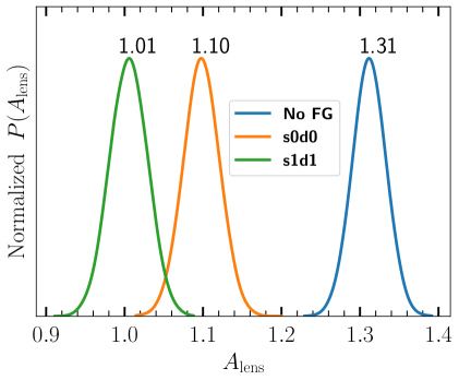
Figure 7: Posterior distribution of $A_{\mathrm{lens}}$ when estimating it for realizations of the s1d1 simulation. The blue curve represents the bias in $A_{\mathrm{lens}}$ when employing the no foreground simulation set to fit the selected spectra. Similarly, the orange and green posterior distributions represent cases where the s0d0 and s1d1 models were used, respectively. The estimated $A_{\mathrm{lens}}$ for each case are quoted at the respective peak of posterior.

Figure 7 presents the posterior distributions of $A_{\mathrm{lens}}$ assuming that s1d1 is real data. The blue posterior corresponds to the estimation of $A_{\mathrm{lens}}$ when assuming no foregrounds, resulting in a bias of $30$%. This bias reduces to $10$% when we utilize the s0d0 model, but is larger than the $1\sigma$ statistical error. This is because the two models, s0d0 and s1d1, have significant discrepancies already in the $EE$ and $BB$ power spectra, as we show in Fig. 1. This discrepancy leads to a significant mismatch between the true and simulation disconnected bias. In practice, however, we would not use no-foreground or s0d0 for our model since it does not fit the data of $EE$ and $BB$ power spectra. Thus, the bias shown here is more enhanced than what would be obtained in an analysis of real data. We finally mention when we correctly use the simulation from the s1d1 model. The bias in $A_{\mathrm{lens}}$ is negligible compared to $\sigma(A_{\rm lens})$, indicating that potential biases other than those considered in the power spectrum estimation are negligible.

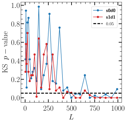
Figure 8: The Kolmogorov-Smirnov test $p$-values obtained for each bin. The red and blue lines represent the $p$-values when comparing s0d0 and s1d1 with the no-foreground case.

To investigate the agreement of the estimated lensing potential angular power spectra between our simulation sets and detect potential biases in our analysis, we apply the Kolmogorov-Smirnov (KS) test to compute $p$-values within each multipole bin of the angular power spectra. The $p$-values are calculated under the null hypothesis that the power spectra for both no-foreground and foreground cases follow the same distribution after bias mitigation (see Eq. 4.6). The $p$-values for both foreground cases, s0d0 and s1d1 are shown in Fig 8. For both foreground cases, the $p$-values for angular scales below $L=400$ exceeded the $0.05$ threshold, indicating a consistent distribution with the no-foreground case. However, for angular scales beyond $L=400$, the $p$-values fell below $0.05$, suggesting a significant deviation. This deviation can be attributed to the non-negligible disconnected bias present in the foreground cases. Despite the discrepancies at high $L$, our analysis demonstrates the effective recovery of the lensing power spectrum, particularly within the angular scales of $L\leq 400$, where the lensing signal dominates.

5 Applications of LiteBIRD Lensing Map

In this Section, we discuss some of the potential applications of the LiteBIRD lensing map.

5.1 Cross-correlations

One potential application of the LiteBIRD CMB lensing map is to cross-correlate it with other tracers of the large-scale structures in the Universe. The full-sky LiteBIRD lensing map can be used to calibrate tracers of the large-scale structure through cross-correlation and hence to constrain cosmology. Here, to estimate the SNR of the cross-correlation signal, we use the following equation:

$$({\rm SNR})^{2}=\sum_{L=L_{\rm min}}^{L_{\rm max}}\frac{f_{\rm sky}^{XY}(2L+1)\left(C^{XY}_{L}\right)^{2}}{\left(C^{XY}_{L}\right)^{2}+\left(C^{XX}_{L}+N_{L}^{XX}\right)\left(C^{YY}_{L}+N_{L}^{YY}\right)}\,,$$ (5.1)

where $X$ and $Y$ represent the observables as specified below, $N_{L}^{XX}$ and $N_{L}^{YY}$ are the associated noise power spectra, and $f_{\rm sky}^{XY}$ is the sky fraction of the overlapping patch of the two observables. In this work, we use the baseline noise model, obtained with the s1d1 simulations (as described in Section 3). We do not consider potential biases arising from the bispectrum of the lensing potential, which only leads to a sub-percent level of bias using the $EB$ estimator, even for high-resolution experiments, as shown in Ref. [125].

5.1.1 Galaxy-lensing cross-correlation as a probe of primordial non-Gaussianity

The fluctuations of the galaxy number density trace the underlying matter distribution of the large-scale structure and efficiently correlate with the CMB lensing maps. We estimate the SNR of the galaxy-CMB lensing cross-correlation signal ($C^{\phi{\rm g}}_{L}$) for two different galaxy surveys: the one provided by Euclid [126] and the one from the Vera C. Rubin Observatory’s Legacy Survey of Space and Time (LSST, [127]). To compute the total SNR, we consider a range of multipoles $L=[2,1000]$. For the Euclid survey, we consider ten equipopulated tomographic galaxy bins and $f_{\rm sky}^{\phi{\rm g}}=0.36$, obtaining ${\rm SNR}=73$. For the LSST survey, we consider ten equispaced redshift bins and $f_{\rm sky}^{\phi{\rm g}}=0.35$, obtaining ${\rm SNR}=56$. Through the cross-correlation analysis between CMB lensing and galaxy distributions, we can constrain the local primordial non-Gaussianity $f_{\rm NL}$, which induces a scale-dependent bias due to the coupling between long and short wavelength modes (e.g., Refs. [128, 129, 130, 131]). To determine the uncertainty of $f_{\rm NL}$ using the cross-spectrum $C^{\phi{\rm g}}_{L}$ alone, we perform a $\chi^{2}$ analysis in which we let only $f_{\rm NL}$ free to vary. When considering the cross-correlation between Euclid galaxies and LiteBIRD CMB lensing, the resulting constraints on $f_{\rm NL}$ are $\sigma(f_{\rm NL})=44$. Note that in this analysis, we vary only $f_{\rm NL}$, and therefore, we do not explore potential degeneracies with other cosmological parameters.

5.1.2 CIB-lensing cross-correlation

The cosmic infrared background (CIB) is the integrated emission from unresolved dusty star-forming galaxies. Produced by the stellar-heated dust within galaxies, the CIB carries a wealth of information about the star formation process. The CIB traces the matter distribution at a relatively high redshift compared to galaxies in typical optical redshift surveys and is strongly correlated with CMB lensing. This cross-correlation can be used to constrain CIB models [132] and cosmology [133]. Planck has measured the CIB-lensing cross-correlations with an SNR of $40$ (statistical uncertainties only) [45]. We estimate the SNR of the CIB-lensing cross-correlation, assuming the CIB anisotropies measured by Planck  which utilizes the model of CIB described in Appendix D of Ref. [64]. We choose $L_{\rm min}=100$ due to a contaminant from residual foregrounds in the CIB map. We find that the SNR of the cross-correlation is $79$ with $f_{\rm sky}^{\phi I}=0.60$, which is roughly a factor of two improvement compared with obtained by Planck.

5.1.3 ISW-lensing cross-correlation

The ISW effect provides information on large-scale structure through large-scale temperature fluctuations [134]. As the same structure generates both the CMB lensing potential and the ISW effect, a substantial cross-correlation between the two observables is expected [135]. The cross-correlation between ISW and CMB lensing is only significant at low multipoles (see, e.g., Ref. [97]). Thus, to measure the cross-correlation with the ISW effect, we need a nearly full-sky observation of the lensing map from space, such as Planck and LiteBIRD. We compute the SNR of the ISW-lensing cross-correlation signal, $C_{\ell}^{\phi T}$, assuming cosmic-variance limited temperature fluctuations and $f_{\rm sky}^{\phi T}=0.80$. The estimated SNR for our baseline case is approximately $4$.

5.2 Constraints on tensor-to-scalar ratio by delensing

Finally, we can use the internally reconstructed lensing potential for delensing. However, the lensing map of LiteBIRD does not significantly improve the constraint on this tensor-to-scalar ratio as shown in LB-Delensing. The improvement on this constraint is only at the level of a few percent if we use the LiteBIRD lensing map (see LB-Delensing for the details).

6 Summary and Discussion

We have conducted a lensing reconstruction study assuming the LiteBIRD experimental configuration, focusing on the impact of Galactic foregrounds from synchrotron and dust emission on the lensing analysis. We performed component separation on the frequency maps, applied filtering to the post-component-separated maps, and estimated the lensing potential map. We showed that the foreground-induced mean field and trispectrum have negligible biases on the measurement of the lensing power spectrum. Furthermore, we showed that the SNR of the LiteBIRD lensing map is approximately 40 which is comparable to that obtained from the latest Planck measurement. The LiteBIRD lensing map additionally holds potential for several cross-correlation analyses.

We focused on the lensing reconstruction from LiteBIRD data alone, but we can add Planck data to provide a more precise lensing map over the full sky, which will be investigated in future work. We assumed homogeneous white noise, but the LiteBIRD noise is inhomogeneous due to the scan strategy. This effect could introduce a larger mean-field bias [81, 40]. However, the $EB$ estimator has no significant mean-field bias due to the parity symmetry [79, 136]. The inhomogeneous noise makes the reconstruction sub-optimal without including its effect in the analysis. However, we can optimally perform component-separation and lensing analysis by modifying the covariance matrix, including the inhomogeneity of the noise [40]. For the optimal lensing analysis, we can also incorporate the spatial variation in the estimator normalization [137]. We have also ignored the instrumental systematic effect of the LiteBIRD experiment. Beam systematics could be one of the main sources of biases in the lensing measurement since the lensing analysis uses smaller scales available for a given dataset. These practical issues, including an optimal analysis for inhomogeneous noise and residual foregrounds, and instrumental systematics, will be investigated in our future works. The software used for this study is publicly available at https://github.com/litebird/LiteBIRD-lensing.

Appendix A Constraint on $A_{\mathrm{lens}}$

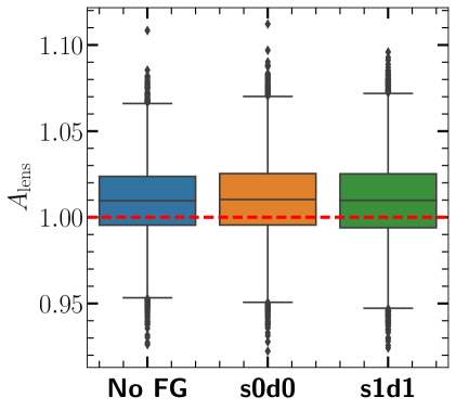
Figure 9: Box plots showing the distribution of samples, with blue, orange, and green denoting the no-foreground, s0d0, and s1d1 cases, respectively. A red dashed line serves as the reference value, indicating $A_{\mathrm{lens}}=1$. Within each box plot, a box spans from the first quartile to the third quartile, while a horizontal black line extends through the box at the median. Lower and upper whiskers correspond to $4\,\sigma$, and individual points denote outliers ($\geq 4\,\sigma$).

This appendix shows some details on estimating $A_{\rm lens}$. We first note that Eq. (4.8) is motivated by the following likelihood:

$$-2\ln(\mathcal{L})=\sum_{bb^{\prime}}\left(\hat{C}_{b}^{\phi\phi}-A_{\rm lens}C_{b}^{\phi\phi,{\rm theory}}\right)\{\mathbf{Cov}^{-1}\}_{bb^{\prime}}\left(\hat{C}_{b^{\prime}}^{\phi\phi}-A_{\rm lens}C_{b^{\prime}}^{\phi\phi,{\rm theory}}\right)\,.$$ (A.1)

Differentiating the above likelihood in terms of $A_{\rm lens}$ leads to Eq. (4.8). Instead of using Eq. (4.8), we can also estimate $A_{\rm lens}$ by maximizing the above likelihood. For example, Fig. 9 shows the results with an Affine-Invariant Markov Chain Monte Carlo (MCMC) Ensemble sampler implemented in Python package emcee for three different foreground cases. Note that the estimated $A_{\rm lens}$ values are in agreement with $A_{\mathrm{lens}}=1$ within the statistical errors. This highlights the agreement between our reconstructed lensing power spectrum in Eq. (4.6) and the theoretical input power spectrum.

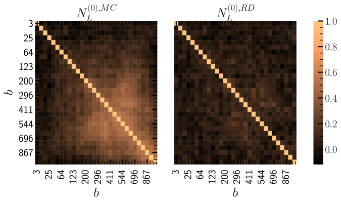
Figure 10: Correlation matrix of the binned angular power spectra for the s1d1 case. The left panel represents results obtained using MCN0, while the right panel illustrates outcomes with RDN0. Notably, the utilization of RDN0 leads to a reduction in correlations within the angular power spectra.

To create the covariance matrix $\mathbf{Cov}$, one can use MCN0 into Eq. (4.6) as the estimate of the disconnected bias. However, this choice introduces correlations within the covariance matrix, which, in turn, influences the precision of the SNR estimation (e.g., Refs. [123, 61, 124]). Instead, RDN0 has been used to reduce these correlations. For the LiteBIRD case, this reduction becomes visually evident when examining the correlation matrix shown in Fig. 10.

References

- [1] M. Zaldarriaga and U. Seljak, An all sky analysis of polarization in the microwave background, Phys. Rev. D D55 (1997) 1830 [astro-ph/9609170].
- [2] M. Kamionkowski, A. Kosowsky and A. Stebbins, Statistics of cosmic microwave background polarization, Phys. Rev. D 55 (1997) 7368.
- [3] U. Seljak, Measuring polarization in cosmic microwave background, Astrophys. J. 482 (1997) 6 [astro-ph/9608131].
- [4] U. Seljak and M. Zaldarriaga, Signature of gravity waves in polarization of the microwave background, Phys. Rev. Lett. 78 (1997) 2054 [astro-ph/9609169].
- [5] M. Kamionkowski, A. Kosowsky and A. Stebbins, A Probe of primordial gravity waves and vorticity, Phys. Rev. Lett. 78 (1997) 2058 [astro-ph/9609132].
- [6] LiteBIRD collaboration, Probing Cosmic Inflation with the LiteBIRD Cosmic Microwave Background Polarization Survey, Prog. Theor. Exp. Phys. 2023 (2023) 042F01 [2202.02773].
- [7] M. Zaldarriaga and U. Seljak, Gravitational lensing effect on cosmic microwave background polarization, Phys. Rev. D 58 (1998) 023003 [astro-ph/9803150].
- [8] K.M. Smith, O. Zahn and O. Dore, Detection of gravitational lensing in the cosmic microwave background, Phys. Rev. D 76 (2007) 043510 [0705.3980].
- [9] C.M. Hirata, S. Ho, N. Padmanabhan, U. Seljak and N.A. Bahcall, Correlation of CMB with large-scale structure: II. Weak lensing, Phys. Rev. D 78 (2008) 043520 [0801.0644].
- [10] F. Bianchini et al., Cross-correlation between the CMB lensing potential measured by Planck and high-z sub-mm galaxies detected by the Herschel-ATLAS survey, Astrophys. J. 802 (2015) 64 [1410.4502].
- [11] DES collaboration, CMB lensing tomography with the DES Science Verification galaxies, Mon. Not. R. Astron. Soc. 456 (2016) 3213 [1507.05551].
- [12] S. Singh, R. Mandelbaum and J.R. Brownstein, Cross-correlating Planck CMB lensing with SDSS: Lensing-lensing and galaxy-lensing cross-correlations, Mon. Not. R. Astron. Soc. 464 (2017) 2120 [1606.08841].
- [13] DES, SPT collaboration, Dark Energy Survey Year 1 Results: Tomographic cross-correlations between Dark Energy Survey galaxies and CMB lensing from South Pole Telescope+Planck, Phys. Rev. D 100 (2019) 043501 [1810.02342].
- [14] POLARBEAR collaboration, Cross-correlation of POLARBEAR CMB Polarization Lensing with High- Sub-mm Herschel-ATLAS galaxies, Astrophys. J. 886 (2019) 38 [1903.07046].
- [15] G.A. Marques and A. Bernui, Tomographic analyses of the CMB lensing and galaxy clustering to probe the linear structure growth, J. Cosmol. Astropart. Phys. 05 (2020) 052 [1908.04854].
- [16] O. Darwish, M.S. Madhavacheril, B. Sherwin, S. Aiola, N. Battaglia, J.A. Beall et al., The Atacama Cosmology Telescope: A CMB lensing mass map over 2100 square degrees of sky and its cross-correlation with BOSS-CMASS galaxies, Mon. Not. R. Astron. Soc. 500 (2020) 2250 [2004.01139].
- [17] A. Krolewski, S. Ferraro and M. White, Cosmological constraints from unWISE and Planck CMB lensing tomography, J. Cosmol. Astropart. Phys. 12 (2021) 028 [2105.03421].
- [18] F. Dong, P. Zhang, L. Zhang, J. Yao, Z. Sun, C. Park et al., Detection of a Cross-correlation between Cosmic Microwave Background Lensing and Low-density Points, Astrophys. J. 923 (2021) 153 [2107.08694].
- [19] Z. Sun, J. Yao, F. Dong, X. Yang, L. Zhang and P. Zhang, Cross-correlation of Planck cosmic microwave background lensing with DESI galaxy groups, Mon. Not. R. Astron. Soc. 511 (2022) 3548 [2109.07387].
- [20] H. Miyatake, Y. Harikane, M. Ouchi, Y. Ono, N. Yamamoto, A.J. Nishizawa et al., First Identification of a CMB Lensing Signal Produced by 1.5 Million Galaxies at z4: Constraints on Matter Density Fluctuations at High Redshift, Phys. Rev. Lett. 129 (2022) 061301 [2103.15862].
- [21] C.S. Saraf, P. Bielewicz and M. Chodorowski, Cross-correlation between Planck CMB lensing potential and galaxy catalogues from HELP, Mon. Not. R. Astron. Soc. 515 (2022) 1993 [2106.02551].
- [22] DES, SPT collaboration, Joint analysis of Dark Energy Survey Year 3 data and CMB lensing from SPT and Planck. I. Construction of CMB lensing maps and modeling choices, Phys. Rev. D 107 (2023) 023529 [2203.12439].
- [23] DES, SPT collaboration, Joint analysis of Dark Energy Survey Year 3 data and CMB lensing from SPT and Planck. II. Cross-correlation measurements and cosmological constraints, Phys. Rev. D 107 (2023) 023530 [2203.12440].
- [24] G. Piccirilli, M. Migliaccio, E. Branchini and A. Dolfi, A cross-correlation analysis of CMB lensing and radio galaxy maps, Astron. Astrophys. 671 (2023) A42 [2208.07774].
- [25] J. Yao et al., KiDS-1000: cross-correlation with Planck cosmic microwave background lensing and intrinsic alignment removal with self-calibration, Astron. Astrophys. 673 (2023) A111 [2301.13437].
- [26] ACT collaboration, The Atacama Cosmology Telescope: Cosmology from cross-correlations of unWISE galaxies and ACT DR6 CMB lensing, (2023) [2309.05659].
- [27] G.S. Farren, B.D. Sherwin, B. Bolliet, T. Namikawa, S. Ferraro and A. Krolewski, Detection of the CMB lensing – galaxy bispectrum, (2023) [2311.04213].
- [28] N. Hand, A. Leauthaud, S. Das, B.D. Sherwin, G.E. Addison, J.R. Bond et al., First measurement of the cross-correlation of CMB lensing and galaxy lensing, Phys. Rev. D 91 (2015) 062001 [1311.6200].
- [29] DES collaboration, Cross-correlation of gravitational lensing from DES Science Verification data with SPT and Planck lensing, Mon. Not. R. Astron. Soc. 459 (2016) 21 [1512.04535].
- [30] J. Liu and J.C. Hill, Cross-correlation of Planck CMB Lensing and CFHTLenS Galaxy Weak Lensing Maps, Phys. Rev. D 92 (2015) 063517 [1504.05598].
- [31] J. Harnois-Déraps et al., CFHTLenS and RCSLenS Cross-Correlation with Planck Lensing Detected in Fourier and Configuration Space, Mon. Not. R. Astron. Soc. 460 (2016) 434 [1603.07723].
- [32] J. Harnois-Déraps et al., KiDS-450: tomographic cross-correlation of galaxy shear with Planck lensing, Mon. Not. R. Astron. Soc. 471 (2017) 1619 [1703.03383].
- [33] DES, SPT collaboration, Dark Energy Survey Year 1 Results: Cross-correlation between Dark Energy Survey Y1 galaxy weak lensing and South Pole Telescope +Planck CMB weak lensing, Phys. Rev. D 100 (2019) 043517 [1810.02441].
- [34] POLARBEAR, HSC collaboration, Evidence for the Cross-correlation between Cosmic Microwave Background Polarization Lensing from POLARBEAR and Cosmic Shear from Subaru Hyper Suprime-Cam, Astrophys. J. 882 (2019) 62 [1904.02116].
- [35] N.C. Robertson, D. Alonso, J. Harnois-Déraps, O. Darwish, A. Kannawadi, A. Amon et al., Strong detection of the CMB lensing and galaxy weak lensing cross-correlation from ACT-DR4, Planck Legacy, and KiDS-1000, Astron. Astrophys. 649 (2021) A146 [2011.11613].
- [36] G.A. Marques, J. Liu, K.M. Huffenberger and J. Colin Hill, Cross-correlation between Subaru Hyper Suprime-Cam Galaxy Weak Lensing and Planck Cosmic Microwave Background Lensing, Astrophys. J. 904 (2020) 182 [2008.04369].
- [37] ACT, DES collaboration, Cosmology from Cross-Correlation of ACT-DR4 CMB Lensing and DES-Y3 Cosmic Shear, (2023) [2309.04412].
- [38] Planck Collaboration, Planck 2013 results. XIX. The integrated Sachs-Wolfe effect, Astron. Astrophys. 571 (2014) A19 [1303.5079].
- [39] Planck Collaboration, Planck 2015 results. XXI. The integrated Sachs-Wolfe effect, Astron. Astrophys. 594 (2016) A21 [1502.01595].
- [40] Planck Collaboration, Planck 2018 results. VIII. Gravitational lensing, Astron. Astrophys. 641 (2020) A8 [1807.06210].
- [41] J. Carron, A. Lewis and G. Fabbian, Planck integrated Sachs-Wolfe-lensing likelihood and the CMB temperature, Phys. Rev. D 106 (2022) 103507 [2209.07395].
- [42] J.C. Hill and D.N. Spergel, Detection of thermal SZ-CMB lensing cross-correlation in Planck nominal mission data, J. Cosmol. Astropart. Phys. 02 (2014) 030 [1312.4525].
- [43] F. McCarthy and J.C. Hill, Cross-correlation of the thermal Sunyaev–Zel’dovich and CMB lensing signals in Planck PR4 data with robust CIB decontamination, (2023) [2308.16260].
- [44] G.P. Holder, M.P. Viero, O. Zahn, K.A. Aird, B.A. Benson, S. Bhattacharya et al., A Cosmic Microwave Background Lensing Mass Map and Its Correlation with the Cosmic Infrared Background, Astrophys. J. 771 (2013) L16 [1303.5048].
- [45] Planck Collaboration, Planck 2013 results. XVIII. The gravitational lensing-infrared background correlation, Astron. Astrophys. 571 (2014) A18 [1303.5078].
- [46] D. Hanson, S. Hoover, A. Crites, P.A.R. Ade, K.A. Aird, J.E. Austermann et al., Detection of B-mode Polarization in the Cosmic Microwave Background with Data from the South Pole Telescope, Phys. Rev. Lett. 111 (2013) 141301 [1307.5830].
- [47] POLARBEAR collaboration, Evidence for Gravitational Lensing of the Cosmic Microwave Background Polarization from Cross-Correlation with the Cosmic Infrared Background, Phys. Rev. Lett. 112 (2014) 131302 [1312.6645].
- [48] ACT collaboration, The Atacama Cosmology Telescope: Lensing of CMB Temperature and Polarization Derived from Cosmic Infrared Background Cross-Correlation, Astrophys. J. 808 (2015) 7 [1412.0626].
- [49] Y. Cao, Y. Gong, C. Feng, A. Cooray, G. Cheng and X. Chen, Cross-Correlation of Far-Infrared Background Anisotropies and CMB Lensing from Herschel and Planck satellites, Astrophys. J. 901 (2020) 34 [1912.12840].
- [50] M.H. Kesden, A. Cooray and M. Kamionkowski, Separation of gravitational wave and cosmic shear contributions to cosmic microwave background polarization, Phys. Rev. Lett. 89 (2002) 011304 [astro-ph/0202434].
- [51] U. Seljak and C.M. Hirata, Gravitational lensing as a contaminant of the gravity wave signal in cmb, Phys. Rev. D 69 (2004) 043005 [astro-ph/0310163].
- [52] K.M. Smith, D. Hanson, M. LoVerde, C.M. Hirata and O. Zahn, Delensing CMB Polarization with External Datasets, J. Cosmol. Astropart. Phys. 06 (2012) 014 [1010.0048].
- [53] T. Okamoto and W. Hu, CMB Lensing Reconstruction on the Full Sky, Phys. Rev. D 67 (2003) 083002 [astro-ph/0301031].
- [54] W. Hu and T. Okamoto, Mass reconstruction with cmb polarization, Astrophys. J. 574 (2002) 566 [astro-ph/0111606].
- [55] S. Das, B.D. Sherwin, P. Aguirre, J.W. Appel, J.R. Bond, C.S. Carvalho et al., Detection of the Power Spectrum of Cosmic Microwave Background Lensing by the Atacama Cosmology Telescope, Phys. Rev. Lett. 107 (2011) 021301 [1103.2124].
- [56] B.D. Sherwin et al., Evidence for dark energy from the cosmic microwave background alone using the atacama cosmology telescope lensing measurements, Phys. Rev. Lett. 107 (2011) 021302 [1105.0419].
- [57] B.D. Sherwin, A. van Engelen, N. Sehgal, M. Madhavacheril, G.E. Addison, S. Aiola et al., The Atacama Cosmology Telescope: Two-Season ACTPol Lensing Power Spectrum, Phys. Rev. D 95 (2017) 123529 [1611.09753].
- [58] ACT collaboration, The Atacama Cosmology Telescope: A Measurement of the DR6 CMB Lensing Power Spectrum and its Implications for Structure Growth, 2304.05202.
- [59] ACT collaboration, The Atacama Cosmology Telescope: DR6 Gravitational Lensing Map and Cosmological Parameters, 2304.05203.
- [60] ACT collaboration, The Atacama Cosmology Telescope: Mitigating the impact of extragalactic foregrounds for the DR6 CMB lensing analysis, 2304.05196.
- [61] Bicep2 / Keck Array Collaboration, BICEP2 / Keck Array VIII: Measurement of gravitational lensing from large-scale B-mode polarization, Astrophys. J. 833 (2016) 228 [1606.01968].
- [62] Bicep2 / Keck Array Collaboration, BICEP / Keck XVII: Line of Sight Distortion Analysis: Estimates of Gravitational Lensing, Anisotropic Cosmic Birefringence, Patchy Reionization, and Systematic Errors, (2022) [2210.08038].
- [63] Planck Collaboration, Planck 2013 results. XVII. Gravitational lensing by large-scale structure, Astron. Astrophys. 571 (2014) A17 [1303.5077].
- [64] Planck Collaboration, Planck 2015 results. XV. Gravitational lensing, Astron. Astrophys. 594 (2015) A15 [1502.01591].
- [65] J. Carron, M. Mirmelstein and A. Lewis, CMB lensing from Planck PR4 maps, J. Cosmol. Astropart. Phys. 09 (2022) 039 [2206.07773].
- [66] POLARBEAR collaboration, Measurement of the Cosmic Microwave Background Polarization Lensing Power Spectrum with the POLARBEAR experiment, Phys. Rev. Lett. 113 (2014) 021301 [1312.6646].
- [67] POLARBEAR collaboration, Measurement of the Cosmic Microwave Background Polarization Lensing Power Spectrum from Two Years of POLARBEAR Data, Astrophys. J. 893 (2020) 85 [1911.10980].
- [68] A. van Engelen, R. Keisler, O. Zahn, K.A. Aird, B.A. Benson, L.E. Bleem et al., A Measurement of Gravitational Lensing of the Microwave Background Using South Pole Telescope Data, Astrophys. J. 756 (2012) 142 [1202.0546].
- [69] K.T. Story, D. Hanson, P.A.R. Ade, K.A. Aird, J.E. Austermann, J.A. Beall et al., A measurement of the cosmic microwave background gravitational lensing potential from 100 square degrees of sptpol data, Astrophys. J. 810 (2015) 50.
- [70] W.L.K. Wu et al., A Measurement of the Cosmic Microwave Background Lensing Potential and Power Spectrum from 500 deg2 of SPTpol Temperature and Polarization Data, Astrophys. J. 884 (2019) 70 [1905.05777].
- [71] M. Millea et al., Optimal Cosmic Microwave Background Lensing Reconstruction and Parameter Estimation with SPTpol Data, Astrophys. J. 922 (2021) 259 [2012.01709].
- [72] SPT collaboration, A Measurement of Gravitational Lensing of the Cosmic Microwave Background Using SPT-3G 2018 Data, 2308.11608.
- [73] Simons Observatory Collaboration, The Simons Observatory: Science goals and forecasts, J. Cosmol. Astropart. Phys. 02 (2019) 056 [1808.07445].
- [74] CMB-S4 Collaboration, CMB-S4 Science Case, Reference Design, and Project Plan, arXiv:1907.04473 (2019) [1907.04473].
- [75] J. Liu, Z. Sun, J. Han, J. Carron, J. Delabrouille, S. Li et al., Forecasts on CMB lensing observations with AliCPT-1, Sci. China Phys. Mech. Astron. 65 (2022) 109511 [2204.08158].
- [76] L. Perotto, J. Bobin, S. Plaszczynski, J.L. Starck and A. Lavabre, Reconstruction of the CMB lensing for Planck, (2009) [0903.1308].
- [77] S. Plaszczynski, A. Lavabre, L. Perotto and J.L. Starck, A hybrid approach to CMB lensing reconstruction on all-sky intensity maps, Astron. Astrophys. 544 (2012) A27 [1201.5779].
- [78] T. Namikawa, D. Hanson and R. Takahashi, Bias-Hardened CMB Lensing, Mon. Not. R. Astron. Soc. 431 (2013) 609 [1209.0091].
- [79] T. Namikawa and R. Takahashi, Bias-hardened CMB lensing with polarization, Monthly Notices of the Royal Astronomical Society 438 (2013) 1507 [1310.2372].
- [80] A. Benoit-Levy, T. Dechelette, K. Benabed, J.-F. Cardoso, D. Hanson and S. Prunet, Full-sky CMB lensing reconstruction in presence of sky-cuts, Astron. Astrophys. 555 (2013) A37 [1301.4145].
- [81] D. Hanson, G. Rocha and K. Gorski, Lensing reconstruction from PLANCK sky maps: inhomogeneous noise, Mon. Not. R. Astron. Soc. 400 (2009) 2169 [0907.1927].
- [82] S.J. Osborne, D. Hanson and O. Dore, Extragalactic Foreground Contamination in Temperature-based CMB Lens Reconstruction, J. Cosmol. Astropart. Phys. 03 (2014) 024 [1310.7547].
- [83] E. Schaan and S. Ferraro, Foreground-Immune Cosmic Microwave Background Lensing with Shear-Only Reconstruction, Phys. Rev. Lett. 122 (2019) 181301 [1804.06403].
- [84] N. Mishra and E. Schaan, Bias to CMB lensing from lensed foregrounds, Phys. Rev. D 100 (2019) 123504 [1908.08057].
- [85] N. Sailer, E. Schaan and S. Ferraro, Lower bias, lower noise CMB lensing with foreground-hardened estimators, Phys. Rev. D 102 (2020) 063517 [2007.04325].
- [86] D. Han and N. Sehgal, Mitigating foreground bias to the CMB lensing power spectrum for a CMB-HD survey, Phys. Rev. D 105 (2022) 083516 [2112.02109].
- [87] O. Darwish, B.D. Sherwin, N. Sailer, E. Schaan and S. Ferraro, Optimizing foreground mitigation for CMB lensing with combined multifrequency and geometric methods, Phys. Rev. D 107 (2023) 043519.
- [88] N. Sailer, S. Ferraro and E. Schaan, Foreground-immune CMB lensing reconstruction with polarization, Phys. Rev. D (2022) [2211.03786].
- [89] F.J. Qu, A. Challinor and B.D. Sherwin, CMB lensing with shear-only reconstruction on the full sky, Phys. Rev. D 108 (2023) 063518 [2208.14988].
- [90] M. Mirmelstein, G. Fabbian, A. Lewis and J. Peloton, Instrumental systematics biases in CMB lensing reconstruction: A simulation-based assessment, Phys. Rev. D 103 (2021) 123540 [2011.13910].
- [91] R. Nagata and T. Namikawa, A numerical study of observational systematic errors in lensing analysis of CMB polarization, Prog. Theor. Exp. Phys. 2021 (2021) 053 [2102.00133].
- [92] D. Beck, J. Errard and R. Stompor, Impact of Polarized Galactic Foreground Emission on CMB Lensing Reconstruction and Delensing of B-Modes, J. Cosmol. Astropart. Phys. 06 (2020) 030 [2001.02641].
- [93] T. Namikawa, A. Lonappan et al., , in prep. (2023) .
- [94] Planck Collaboration, Planck 2018 results. VI. Cosmological parameters, Astron. Astrophys. 641 (2020) A6 [1807.06209].
- [95] M. Tegmark, A. de Oliveira-Costa and A.J.S. Hamilton, High resolution foreground cleaned CMB map from WMAP, Phys. Rev. D 68 (2003) .
- [96] A. Challinor and G. Chon, Geometry of weak lensing of CMB polarization, Phys. Rev. D 66 (2002) 127301 [astro-ph/0301064].
- [97] A. Lewis and A. Challinor, Weak gravitational lensing of the CMB, Phys. Rep. 429 (2006) 1 [astro-ph/0601594].
- [98] D. Hanson, A. Challinor and A. Lewis, Weak lensing of the CMB, Gen. Rel. Grav. 42 (2010) 2197 [0911.0612].
- [99] B. Hadzhiyska, D. Spergel and J. Dunkley, Small-scale modification to the lensing kernel, Phys. Rev. D 97 (2018) 043521 [1711.03168].
- [100] G. Pratten and A. Lewis, Impact of post-born lensing on the cmb, J. Cosmol. Astropart. Phys. 08 (2016) 047 [1605.05662].
- [101] A. Lewis and G. Pratten, Effect of lensing non-Gaussianity on the CMB power spectra, J. Cosmol. Astropart. Phys. 12 (2016) 003 [1608.01263].
- [102] G. Fabbian, M. Calabrese and C. Carbone, CMB weak-lensing beyond the Born approximation: a numerical approach, J. Cosmol. Astropart. Phys. 1802 (2018) 050 [1702.03317].
- [103] T. Namikawa, Cosmology from weak lensing of CMB, Prog. Theor. Exp. Phys. 2014 (2014) 06B108 [1403.3569].
- [104] M. Zaldarriaga and U. Seljak, Gravitational lensing effect on cosmic microwave background polarization, Phys. Rev. D 58 (1998) 023003 [astro-ph/9803150].
- [105] A. Lewis, A. Challinor and D. Hanson, The shape of the CMB lensing bispectrum, J. Cosmol. Astropart. Phys. 03 (2011) 018 [1101.2234].
- [106] E. Komatsu, New physics from the polarized light of the cosmic microwave background, Nature Rev. Phys. 4 (2022) 452 [2202.13919].
- [107] T. Namikawa, CMB mode coupling with isotropic polarization rotation, Mon. Not. Roy. Astron. Soc. 506 (2021) 1250 [2105.03367].
- [108] K.M. Smith et al., CMBPol Mission Concept Study: Gravitational Lensing, AIP Conf. Proc. 1141 (2009) 121 [0811.3916].
- [109] N. Macellari, E. Pierpaoli, C. Dickinson and J.E. Vaillancourt, Galactic foreground contributions to the 5-year Wilkinson Microwave Anisotropy Probe maps, Monthly Notices of the Royal Astronomical Society 418 (2011) 888 [https://academic.oup.com/mnras/article-pdf/418/2/888/3691294/mnras0418-0888.pdf].
- [110] J. Delabrouille, J.F. Cardoso, M.L. Jeune, M. Betoule, G. Fay and F. Guilloux, A full sky, low foreground, high resolution CMB map from WMAP, Astron. Astrophys. 493 (2009) 835 [0807.0773].
- [111] H.K. Eriksen, I.J. O’Dwyer, J.B. Jewell, B.D. Wandelt, D.L. Larson, K.M. Gorski et al., Power spectrum estimation from high-resolution maps by Gibbs sampling, Astrophys. J. Suppl. 155 (2004) 227 [astro-ph/0407028].
- [112] T. Namikawa, A. Baleato Lizancos, N. Robertson, B.D. Sherwin, A. Challinor, D. Alonso et al., Simons Observatory: Constraining inflationary gravitational waves with multitracer B-mode delensing, Phys. Rev. D 105 (2022) 023511 [2110.09730].
- [113] M. Remazeilles, C. Dickinson, A.J. Banday, M.A. Bigot-Sazy and T. Ghosh, An improved source-subtracted and destriped 408 MHz all-sky map, Mon. Not. R. Astron. Soc. 451 (2015) 4311 [1411.3628].
- [114] C.L. Bennett, D. Larson, J.L. Weiland, N. Jarosik, G. Hinshaw, N. Odegard et al., Nine-year Wilkinson Microwave Anisotropy Probe (WMAP) Observations: Final Maps and Results, Astrophys. J. Suppl. Ser. 208 (2013) 20 [1212.5225].
- [115] M.A. Miville-Deschenes, N. Ysard, A. Lavabre, N. Ponthieu, J.F. Macias-Perez, J. Aumont et al., Separation of anomalous and synchrotron emissions using WMAP polarization data, Astron. Astrophys. 490 (2008) 1093 [0802.3345].
- [116] Planck Collaboration, Planck 2015 results. X. Diffuse component separation: Foreground maps, Astron. Astrophys. 594 (2016) A10 [1502.01588].
- [117] K.M. Górski, E. Hivon, A.J. Banday, B.D. Wandelt, F.K. Hansen, M. Reinecke et al., HEALPix: A Framework for High-Resolution Discretization and Fast Analysis of Data Distributed on the Sphere, Astrophys. J. 622 (2005) 759 [arXiv:astro-ph/0409513].
- [118] M.H. Kesden, A. Cooray and M. Kamionkowski, Lensing reconstruction with CMB temperature and polarization, Phys. Rev. D 67 (2003) 123507 [astro-ph/0302536].
- [119] T. Namikawa, “cmblensplus: A tool to analyze cosmic microwave background anisotropies.” Astrophysics Source Code Library, record ascl:2104.021, Apr., 2021.
- [120] D. Hanson, A. Challinor, G. Efstathiou and P. Bielewicz, Cmb temperature lensing power reconstruction, Phys. Rev. D 83 (2011) 043005 [1008.4403].
- [121] V. Boehm, M. Schmittfull and B. Sherwin, Bias to CMB lensing measurements from the bispectrum of large-scale structure, Phys. Rev. D 94 (2016) 043519 [1605.01392].
- [122] V. Boehm, B.D. Sherwin, J. Liu, J.C. Hill, M. Schmittfull and T. Namikawa, On the effect of non-gaussian lensing deflections on cmb lensing measurements, Phys. Rev. D 98 (2018) 123510 [1806.01157].
- [123] M.M. Schmittfull, A. Challinor, D. Hanson and A. Lewis, Joint analysis of CMB temperature and lensing-reconstruction power spectra, Phys. Rev. D 88 (2013) 063012 [1308.0286].
- [124] J. Peloton, M. Schmittfull, A. Lewis, J. Carron and O. Zahn, Full covariance of CMB and lensing reconstruction power spectra, Phys. Rev. D 95 (2017) 043508 [1611.01446].
- [125] G. Fabbian, A. Lewis and D. Beck, CMB lensing reconstruction biases in cross-correlation with large-scale structure probes, J. Cosmol. Astropart. Phys. 10 (2019) 057 [1906.08760].
- [126] Euclid Collaboration, A. Blanchard, S. Camera, C. Carbone, V.F. Cardone, S. Casas et al., Euclid preparation. VII. Forecast validation for Euclid cosmological probes, Astron. Astrophys. 642 (2020) A191 [1910.09273].
- [127] The LSST Dark Energy Science Collaboration, R. Mandelbaum, T. Eifler, R. Hložek, T. Collett, E. Gawiser et al., The lsst dark energy science collaboration (desc) science requirements document, (2018) .
- [128] N. Dalal, O. Dore, D. Huterer and A. Shirokov, The imprints of primordial non-gaussianities on large-scale structure: scale dependent bias and abundance of virialized objects, Phys. Rev. D 77 (2008) 123514 [0710.4560].
- [129] D. Jeong, E. Komatsu and B. Jain, Galaxy-CMB and galaxy-galaxy lensing on large scales: sensitivity to primordial non-Gaussianity, Phys. Rev. D 80 (2009) 123527 [0910.1361].
- [130] M. Schmittfull and U. Seljak, Parameter constraints from cross-correlation of CMB lensing with galaxy clustering, Phys. Rev. D 97 (2018) 123540 [1710.09465].
- [131] M. Ballardini, W.L. Matthewson and R. Maartens, Constraining primordial non-Gaussianity using two galaxy surveys and CMB lensing, Mon. Not. R. Astron. Soc. 489 (2019) 1950 [1906.04730].
- [132] F. McCarthy and M.S. Madhavacheril, Improving models of the cosmic infrared background using CMB lensing mass maps, Phys. Rev. D 103 (2021) 103515 [2010.16405].
- [133] F. McCarthy, M.S. Madhavacheril and A.S. Maniyar, Constraints on primordial non-Gaussianity from halo bias measured through CMB lensing cross-correlations, Phys. Rev. D 108 (2023) 083522 [2210.01049].
- [134] R.K. Sachs and A.M. Wolfe, Perturbations of a Cosmological Model and Angular Variations of the Microwave Background, Astrophys. J. 147 (1967) 73.
- [135] D.M. Goldberg and D.N. Spergel, Microwave background bispectrum. 2. A probe of the low redshift universe, Phys. Rev. D 59 (1999) 103002 [astro-ph/9811251].
- [136] R. Pearson, B. Sherwin and A. Lewis, CMB lensing reconstruction using cut sky polarization maps and pure- modes, Phys. Rev. D 90 (2014) 023539 [1403.3911].
- [137] M. Mirmelstein, J. Carron and A. Lewis, Optimal filtering for CMB lensing reconstruction, Phys. Rev. D 100 (2019) 123509 [1909.02653].