Onflow: an online portfolio allocation algorithm

Abstract

We introduce Onflow, a reinforcement learning technique that enables online optimization of portfolio allocation policies based on gradient flows. We devise dynamic allocations of an investment portfolio to maximize its expected log return while taking into account transaction fees. The portfolio allocation is parameterized through a softmax function, and at each time step, the gradient flow method leads to an ordinary differential equation whose solutions correspond to the updated allocations. This algorithm belongs to the large class of stochastic optimization procedures; we measure its efficiency by comparing our results to the mathematical theoretical values in a log-normal framework and to standard benchmarks from the ’old NYSE’ dataset.

For log-normal assets, the strategy learned by Onflow, with transaction costs at zero, mimics Markowitz’s optimal portfolio and thus the best possible asset allocation strategy. Numerical experiments from the ’old NYSE’ dataset show that Onflow leads to dynamic asset allocation strategies whose performances are: a) comparable to benchmark strategies such as Cover’s Universal Portfolio or Helmbold et al. "multiplicative updates" approach when transaction costs are zero, and b) better than previous procedures when transaction costs are high. Onflow can even remain efficient in regimes where other dynamical allocation techniques do not work anymore.

Therefore, as far as tested, Onflow appears to be a promising dynamic portfolio management strategy based on observed prices only and without any assumption on the laws of distributions of the underlying assets’ returns. In particular it could avoid model risk when building a trading strategy.

1 Motivation and literature review

Ever since the advent of modern portfolio theory, reliable information on the statistical properties of the financial time series is a crucial determinant of the portfolio performance. Formulated in a mean-variance setting, the classical approach of [22] promises optimal performance when the future first and second order moments are known. Or, in general, this information is highly uncertain and in practice the quality of the result is far from the expected level. To cure this empirical drawback, several approaches were proposed: [16] analyzed optimal bet size in investment portfolios, [3] modeled the expected return as variables which are updated, by investor convictions, though a Bayesian mechanism, while [8] introduced the Universal portfolio to profit from the long term exponential behavior and obtain results that are comparable with best constant rebalanced portfolio chosen in hindsight. This latter approach uses no assumption whatsoever on the statistical properties of the asset’s time series and was followed by a large literature aiming to produce performances robust to variations in the model parameters. Among such follow-ups we will focus on the online learning approaches which enters the general framework of reinforcement learning, where data is fed directly into a strategy without any model in between. In particular [12] proposed a first version using multiplicative updates and a relative cross-entropy loss function, [19] persisted along these lines assuming a reversion to the mean while [4] explored the theoretical and practical implications of transaction costs while [kirby_low_turnover_12] proposed low turnover strategies. On the other hand, [5] introduced the Anticor algorithm that exploits the general idea of correlation between assets of the pair. For additional findings on online portfolio selection we refer to the reviews of [18], [sato2019modelfree] and [sun_review_rl_trading2023] while for a more machine learning orientation see [6] and [10, Chapter 3]; finally see [20] for an open source toolbox to test algorithms. More recently, [zhang_combining_2021] proposed a strategy combining different experts, [11] made available a literature review and an extension of the Anticor approach using dynamic time warping as similarity distance; [deep_policy_grad_19] investigated policy gradient style deep reinforcement learning approaches and [ngo_does_2023] compared reinforcement learning and deep learning methods in portfolio optimization.

Remaining in this framework of online, no hindsight, reinforcement learning, model-free approaches we present here a algorithm using the gradient flow concept instead of discrete updates that can treat in an intrinsic way the transactions costs. The portfolio allocation is parametrized through a softmax function.

The outline of the paper is the following; in section 2 we introduce the Onflow algorithm; subsequently, in section 3 some theoretical results are presented. In section 4 we test the performance of the procedure on several benchmarks from the literature and in section 5 we conclude with additional remarks.

2 Onflow algorithm : intuition and formal definition

Consider a market $\mathcal{M}$ containing $K$ financial assets and $T$ time instants $t\in\mathcal{T}:=\{1,...,T\}$; $T$ can be either finite or infinite. We denote $S^{k}_{t}$ the value at time $t$ of the asset $k$ and assume $S^{k}_{0}=1,S^{k}_{t}>0,\forall k,t$. The price relatives $f_{t}^{k}$ are defined as $f^{k}_{t}=S^{k}_{t}/S^{k}_{t-1}$, $\forall t\in\mathcal{T}$.

A portfolio is characterized by a set of $K$ weights $\pi=(\pi(1),...,\pi(K))$. At any time $t$ the quotient of the wealth invested in the asset $k$ with respect to total portfolio value is set to $\pi(k)$ which means that the $\pi(k)$ sum up to one. We will suppose that each $\pi(k)$ is positive, i.e., no short selling is allowed. In this case $\pi$ belongs to the unit simplex $\mathcal{S}_{K}$ of dimension $K$ :

$$\mathcal{S}_{K}=\left\{w=(w_{k})_{k=1}^{K}\in\mathbb{R}^{K}:w_{k}\geq 0,\sum_{k=1}^{K}w_{k}=1\right\}.$$ (1)

We will denote $\mathring{\mathcal{S}_{K}}$ the interior of $\mathcal{S}_{K}$ i.e.

$$\mathring{\mathcal{S}_{K}}=\left\{w=(w_{k})_{k=1}^{K}\in\mathbb{R}^{K}:w_{k}>0,\sum_{k=1}^{K}w_{k}=1\right\}.$$ (2)

When $\pi$ is constant in time, we obtain the so called Constant Rebalanced Portfolio (CRP) also called a ’Constant Mix’ portfolio. Note that a CRP is a dynamic investment strategy because the price evolution may induce a shift in the proportions $\pi$ that have to be reset to the prescribed values.

We denote $f_{t}$ the vector with components $f^{k}_{t}$, $k\leq K$, $t\in\mathcal{T}$. A portfolio with initial value $\mathcal{V}_{0}(\pi)$ at $t=0$ and weights $\pi_{t}$ chosen at time $t-1$ has the value $\mathcal{V}_{t}(\pi)$ at time $t$ with :

$$\mathcal{V}_{0}(\pi)=1,\ \forall t\in\mathcal{T}~{}:\mathcal{V}_{t}(\pi)=\mathcal{V}_{0}(\pi)\prod_{s=1}^{t}\langle\pi_{s},f_{s}\rangle=\mathcal{V}_{0}(\pi)e^{\sum_{s=1}^{t}\ln(\langle\pi_{s},f_{s}\rangle)}.$$ (3)

As a side remark, note that formula (3) can also be written

$$\ln(\mathcal{V}_{t}(\pi))=\ln(\mathcal{V}_{0}(\pi))+\sum_{s=1}^{t}\ln(\langle\pi_{s},f_{s}\rangle)=\ln(\mathcal{V}_{0}(\pi))+t\cdot\frac{\sum_{s=1}^{t}\ln(\langle\pi_{s},f_{s}\rangle)}{t},$$ (4)

and, if we interpret $(\pi_{s},f_{s})$ to be samples from some joint distribution denoted $(\pi,f)$ we recognize in $\frac{\sum_{s=1}^{t}\ln(\langle\pi_{s},f_{s}\rangle)}{t}$ an empirical estimator for $\mathbb{E}[\ln(\langle\pi,f\rangle)]$.

2.1 Reinforcement learning framework

Reinforcement learning (abbreviated ’RL’ from now on, see [25, Chapter 3] for a pedagogical introduction) is proved to be very efficient when model-free approaches are necessary for problems involving repeated decisions, such as game play, robot maneuvering, autonomous car driving, etc.

For the reader already versed in reinforcement learning we provide below the transcription of our setting to the formal writing of a RL problem which involves :

• a sequence of time instants: for us will be $\mathcal{T}$

• a state of the world at each time $t$ : for us this will be the allocation $\pi_{t}$ and the portfolio value $\mathcal{V}_{t}(\pi)$

• a set of actions to chose from at time $t$ : for us this is $\mathcal{S}_{K}$ where $\pi_{t+1}$ belongs

• rewards $r_{t}$ obtained at each time $t$ depending on previous actions, see below for the precise choice we make. Note that it is not necessary for the reward $r_{t}$ to result deterministically from the actions.

• a strategy to choose the next action: the general prescription in reinforcement learning is to choose a probability law on the set of actions, i.e., a distribution on $\mathcal{S}_{K}$. However in remark 2 we argue that there is no need to go beyond distributions that are Dirac masses located at some element $\mathcal{S}_{K}$.

Then the problem is formalized as :

$$\textrm{ choose iteratively }\pi_{t+1}\textrm{ to maximize the expected value of the rewards }\mathbb{E}[r_{t}].$$ (5)

Remark 1.

Compared with the reinforcement learning literature we consider that the time is not discounted, i.e., a reward $r$ at time $s$ is worth as much as a reward $r$ at some other time. Such discounting is used often when the quantity to optimize would be infinite but increasing sub-exponentially.

A possible choice for the rewards $r_{t}$ are the portfolio gains from time $t-1$ to $t$. This may not be a good idea because the increase could be exponential and even discounting may not help to make it finite. In view of the relation (3) above and in coherence with existing literature, it is more natural to look for procedures that maximize the expected value of $r_{s}=\ln(\langle\pi_{s},f_{s}\rangle)$; for instance [12] chooses $\pi_{t+1}$ to maximize this expected value using a particular choice of multiplicative updates derived from an approximation of the relative entropy to the first order. We will subscribe to the same convention but we add to $r_{s}$ a term to model the transactions costs as explained below.

Remark 2.

The formula of the reward $\ln(\langle\pi,f_{s}\rangle)$ and the concavity of the logarithm implies by the Jensen inequality that any average of elements in $\mathcal{S}_{K}$ (average following some distribution on $\mathcal{S}_{K}$) will perform worse than their mean. So the optimal distribution on $\mathcal{S}_{K}$ will necessarily be a Dirac mass.

2.2 The onflow algorithm

We therefore look for iterative procedures that starting from the state of the portfolio and of the market $\mathcal{M}$ up to time $t$ adjusts $\pi_{t}$ into some $\pi_{t+1}$ with better expected rewards. On ther other hand, in coherence with the extensive literature on the gradient flows [14], it is natural to also ask $\pi_{t+1}$ to be somehow close to $\pi_{t}$. Various ways to impose this proximity are possible, most of them exploiting the fact that $\pi$ is a discrete probability law on the set $\{1,...,K\}$ for instance [12] uses relative cross-entropy. We will parametrize $\mathcal{S}_{K}$ through the "softmax" function, denoted $S(\cdot)$ and defined by :

$$S:\mathbb{R}^{K}\to\mathcal{S}_{K},\ H\in\mathbb{R}^{K}\mapsto S(H)=\pi\in\mathcal{S}_{K},\pi(k)=\frac{e^{H_{k}}}{\sum_{\ell}e^{H_{\ell}}}.$$ (6)

Remark 3.

A limited amount of short selling can be accommodated by taking as portfolio allocation not $S(H)$ but $\pi_{\lambda}=(1+\lambda)S(H)-\lambda/K$, with $\lambda>0$ a fixed value; the entries sum up to $1$ but $\pi_{\lambda}$ is not always in $\mathcal{S}_{K}$ as it can have negative entries not exceeding $\lambda/K$.

Let us denote with these new variables our reward function :

$$F_{t}(H):=\ln(\langle S(H),f_{t}\rangle).$$ (7)

So, $H_{t+1}$ could be chosen to maximize $F_{t}$ and stay close to $H_{t}$; a good candidate is the minimizer of $\frac{1}{2\tau}\|H-H_{t}\|^{2}-F_{t}(H)$ where the constant $\tau$ has the meaning of a "numerical" time, see [14].

Note that one of the reasons why we want $H_{t+1}$ to stay close to $H_{t}$ is because the transition from $H_{t}$ to $H_{t+1}$ can be costly in terms of transaction fees. We will consider proportional transaction fees that charge a given, known, percentage of the amount sold or bought; note that in this transaction fee model moving an amount $X$ from one asset to the other will cost twice this percentage because both buying and selling are taxed; see also [4] for additional discussions on the transaction fees models and for some optimizations that occur. We will not consider here such buy/sell optimization and to make things comparable with the literature we resume everything to a parameter $\xi>0$ and consider that for a portfolio of value $V$ switching from allocation $\tilde{\pi}$ to $\pi$ costs $\xi V\sum_{k}|\tilde{\pi}(k)-\pi(k)|$.

Also note that the allocation $\pi_{t}$ that was selected at time $t-1$ and before prices at $t$ were known will drift by itself ’overnight’ because of the price evolution given by the price relatives $f_{t}$ ; a simple computation shows that the new allocation that takes into account the prices at time $t$ is :

$$\pi_{t+}=\frac{\pi_{t}\odot f_{t}}{\langle\pi_{t},f_{t}\rangle}=\left(\frac{\pi_{t}(k)f_{t}(k)}{\sum_{\ell}\pi_{t}(\ell)f_{t}(\ell)}\right)_{k=1}^{K},\ \odot=\textrm{ element-wise (Hadamard) product}.$$ (8)

Rebalancing a portfolio of total value $V$ that drifted to $\pi_{t+}$ to the target allocation $\pi$ will lower $V$ to $V-V\xi\sum_{k}|\pi_{t+}(k)-\pi(k)|$ i.e. will act by a multiplication with $1-\xi\sum_{k}|\pi_{t+}(k)-\pi(k)|=e^{\ln(1-\xi\sum_{k}|\pi_{t+}(k)-\pi(k)|)}\simeq e^{-\xi\sum_{k}|\pi_{t+}(k)-\pi(k)|}$ where for the last approximation we used that transaction fee level $\xi$ is small compared to $1$. As a technical detail, the absolute value $|\cdot|$ above is not smooth enough and may induce numerical instabilities in the computations; to avoid this we regularize it to $\sqrt{|\cdot|^{2}+a^{2}}-a$ which is differentiable for any $a>0$ and converges to the absolute value for $a\to 0$; such a function proved to be useful in many areas of machine learning, cf. [7, 26] and is sometime called "pseudo-Huber" loss. For numerical tests we set $a=10^{-6}$.

Recalling that we are maximizing the expectation of the logarithm of the rewards, the transaction fees are therefore modeled as :

$$G_{t}(H):=\xi\sum_{k=1}^{K}\sqrt{[\mathcal{S}(H)(k)-\pi_{t+}(k)]^{2}+a^{2}}-a.$$ (9)

With these provisions one can take $H_{t+1}$ to be a minimizer of $\frac{1}{2\tau}\|H-H_{t}\|^{2}-F_{t}(H)+G_{t}(H)$. All that remains is to choose the value for $\tau$; however, the most adequate value of $\tau$ depends on the statistics of $f_{t}$ and may not be easy to guess from the start. On the other hand, it is known from the classical theory of the gradient flows that for general smooth functions $\mathcal{F}$, setting $H_{t+1}$ as the minimizer of $\frac{1}{2\tau}\|H-H_{t}\|^{2}+\mathcal{F}(H)$ will lead the trajectory $H_{t}$ to converge, when $\tau\to 0$, to the solution of $H(t)^{\prime}=-\nabla\mathcal{F}(H)$; on the contrary when $\tau$ is large such convergence is not assured and instabilities can occur. To cure this potential drawback and be free in the choice of the values $\tau$ we will define $H_{t+1}$ as follows: solve for $u\in[0,\tau]$ the ODE :

$$\mathcal{H}(u=0)=H_{t},\ \frac{d}{du}\mathcal{H}(u)=\nabla_{H}(F_{t}(\mathcal{H}(u))-G_{t}(\mathcal{H}(u))),$$ (10)

then set $H_{t+1}=\mathcal{H}(\tau)$. Replacing the gradients $\nabla_{H}F_{t}$ and $\nabla_{H}G_{t}$ we obtain the following ODE :

$$\begin{cases}\mathcal{H}(u=0)=H_{t}\\ \frac{d}{du}\mathcal{H}(u)=\frac{\mathcal{S}(\mathcal{H}(u))\odot f_{t}}{\langle\mathcal{S}(\mathcal{H}(u)),f_{t}\rangle}-\mathcal{S}(\mathcal{H}(u))\\ -\xi\left(\sum_{k}\frac{\mathcal{S}(\mathcal{H}(u))(k)-\pi_{t+}(k)}{\sqrt{(\mathcal{S}(\mathcal{H}(u))(k)-\pi_{t+}(k))^{2}+a^{2}}}\mathcal{S}(\mathcal{H}(u))(k)(\mathbbm{1}_{k=b}-\mathcal{S}(\mathcal{H}(u))(b))\right)_{b=1}^{K}.\end{cases}$$ (11)

We used here the softmax derivation formula for $S(\cdot)$:

$$\frac{\partial}{\partial H_{b}}S(H)(k)=S(H)(k)(\mathbbm{1}_{k=b}-S(H)(b)).$$ (12)

We can now formally introduce the ’Onflow’ algorithm, described in the pseudo-code below.

Algorithm A1 Onflow portfolio allocation algorithm

Inputs : parameter $\tau>0$, $a$ (default value $a=10^{-6}$).

Outputs : allocations $\pi_{t}$, $t\in\mathcal{T}$.

1:procedure 

2:     Set $t=1$, $H_{t}=0\in\mathbb{R}^{K}$.

3:     for $t\in T$ do

4:         read $f_{t}$, compute $\pi_{t+}$ from (8)

5:         solve ODE (11) and set $H_{t+1}=\mathcal{H}(\tau)$, $\pi_{t+1}=S(H_{t+1})$

6:         store $\pi_{t+1}$

7:     end for

8:end procedure

Remark 4.

In general solving the ODE at line 5 is not difficult because the number of assets is in practice not too large ($2$ to $100$). Should this not be the case, one can try instead an explicit Euler numerical scheme with step $\tau$ which boils down to simple vectors addition.

Remark 5.

For comparison, the $EC(\eta)$ algorithm of [12] use instead an update of the form :

$$H_{t+1}=H_{t}+\tau\frac{f_{t}}{\langle\pi_{t},f_{t}\rangle}+c_{t},$$ (13)

where $c_{t}$ is a constant with respect to $k\leq K$ but that can change with time. It also corresponds to a Natural Policy Gradient (NPG) algorithm, see [2] for the seminal work on the natural gradient and [1, Lemma 15] for its formulation in reinforcement learning under the policy gradient framework.

Remark 6.

The price relatives $f_{t}$ are stochastic in nature and the maximization of the performance needs to take into account this fact. The standard way to deal with such circumstance is to use a stochastic optimization algorithm, variant of the Stochastic Gradient Descent introduced in [24]; see [25] for its use in reinforcement learning in general and [27] for a short self-contained convergence proof. When optimizing a general function $\mathcal{F}(x)$ this optimization algorithm converges even if, instead of the true gradient $\nabla\mathcal{F}(x)$ only a non-biased version is used at each step instead; in practice, to lower the variance of the error, a sample average based on $B$ non-biased gradients can be used. This means that instead of advancing $1$ step at the time one can advance $B$ steps and adapt formula (11) to take into account a sample average of price relatives $f_{t}$,…, $f_{t+B}$. Note that the algorithm, as written above, corresponds to $B=1$.

3 Theoretical convergence results

We present in this section a convergence result which shows that the Onflow algorithm will reach optimality under some special assumptions. More precisely, we will consider the continuous limit i.e., $\mathcal{T}=\mathbb{R}_{+}$, no transaction fees ($\xi=0$) and assume that the asset dynamic is log-normal. Of course, this is a simplification because in real life no asset dynamic is exactly log-normal. But, it is still reassuring that in this prototypical situation our algorithm is consistent and provides the expected solution. As in recent works on the convergence of softmax-formulated reinforcement learning problems, see [23, 1], we will work in the "true gradient" regime.

We use the following notations for the log-normal dynamics of the assets :

$$\frac{dS^{k}_{t}}{S^{k}_{t}}=\mu_{k}dt+\sum_{\ell=1}^{K}\sigma_{k\ell}dz_{\ell}(t),$$ (14)

where $z_{\ell}$ are independent Brownian motions. Note that in general the drifts $\mu=(\mu_{k})_{k=1}^{K}$ and $\sigma=(\sigma_{k\ell})_{k,\ell=1}^{K}$ are unknown. The covariance matrix will be denoted $\Sigma=\sigma^{T}\sigma$. Since for any $T\geq 0$ :

$$\mathbb{E}[\ln(\mathcal{V}_{T}(\pi))]=\mathbb{E}[\ln(\mathcal{V}_{0}(\pi))]+\int_{0}^{T}\frac{d}{dt}\mathbb{E}[\ln(\mathcal{V}_{t}(\pi))]dt,$$ (15)

we can formulate as in [13] the log-optimum portfolio as the continuous maximization over $\mathcal{S}_{K}$ of $\frac{d}{dt}\mathbb{E}[\ln(\mathcal{V}_{t}(\pi))]$ which means that in this setting $F_{t}(H):=\frac{d}{dt}\mathbb{E}[\ln(\mathcal{V}_{t}(S(H)))]$. Or, the Ito formula shows that :

$$F_{t}(H)=R(S(H)),\textrm{ where }R(\pi):=\langle\mu,\pi\rangle-\frac{1}{2}\pi^{T}\Sigma\pi.$$ (16)

Since $\xi=0$ from equations (10) and (16) we obtain that the algorithm corresponds to solving the following ODE :

$$\mathcal{H}(0)=0\in\mathbb{R}^{K},\ \frac{d}{dt}\mathcal{H}(t)=\nabla_{H}R(S(\mathcal{H}(t)))\ \forall t>0.$$ (17)

$$\textrm{Output allocation at time }t~{}:~{}\pi_{t}=S(\mathcal{H}(t)).$$ (18)

On the other hand the optimal allocation $\pi^{\star}$ is the solution of the following problem :

$$\max_{\pi\in\mathcal{S}_{K}}R(\pi).$$ (19)

We will need a notation : suppose $\Sigma$ is non-singular; for any $\mathcal{L}\subset\{1,...,K\},\mathcal{L}\neq\emptyset$ denote by $\Sigma_{\mathcal{L},\mathcal{L}}^{-1}$ the matrix that, restricted to the indices in $\mathcal{L}$ is the inverse of the $\mathcal{L}\times\mathcal{L}$ minor of $\Sigma$ and zero elsewhere .

We give now the main result that shows, under appropriate technical hypothesis, that the output allocation $\pi_{t}$ will converge to the optimum allocation $\pi^{\star}$.

Proposition 1.

In the framework above assume that $\Sigma$ is non-singular. Then :

1. maximization problem (19) has a unique solution $\pi^{\star}\in\mathcal{S}_{K}$;

2. the reward $R_{t}=R(\pi_{t})$ is monotonically increasing;

3. The output allocation $(\pi_{t})_{t\geq 0}$ in (18) converges, we denote $\pi^{\infty}:=\lim_{t\to\infty}\pi_{t}$; in addition

   $$\pi^{\infty}\in\mathcal{S}_{K}\cap\left\{\mathbbm{1}_{\mathcal{L}}\odot\Sigma^{-1}\mu+\frac{1-\langle\mathbbm{1}_{\mathcal{L}},\Sigma^{-1}\mu\rangle}{\langle\mathbbm{1}_{\mathcal{L}},\Sigma_{\mathcal{L},\mathcal{L}}^{-1}\mathbbm{1}_{\mathcal{L}}\rangle}\Sigma_{\mathcal{L},\mathcal{L}}^{-1}\mathbbm{1}_{\mathcal{L}},\mathcal{L}\subset\{1,...,K\},\mathcal{L}\neq\emptyset\right\};$$ (20)

4. there exists $c_{\epsilon}$ depending only on $\Sigma$ and $\mu$ such that if $\|\pi_{0}-\pi^{\star}\|_{\Sigma}\leq c_{\epsilon}$ then $\lim_{t\to\infty}\pi_{t}=\pi^{\star}$;

5. for general initial value $\pi_{0}$, not necessarily close to $\pi^{\star}$, if $\pi^{\infty}\in\mathring{\mathcal{S}_{K}}$ then $\pi^{\star}\in\mathring{\mathcal{S}_{K}}$ and $\lim_{t\to\infty}\pi_{t}=\pi^{\star}$. Moreover, in this case the convergence is exponential i.e. there exists $c_{0},c_{1}>0$ such that :

   $$\|\pi_{t}-\pi^{\star}\|\leq c_{0}e^{-c_{1}t},\ \forall t\geq 0.$$ (21)

Proof.

Proof of step 1 : Note that when $\Sigma$ is non singular the maximum in (19) is necessarily unique because $\Sigma$ will be strictly positive definite so the maximization problem involves a strictly convex function on the closed convex domain $\mathcal{S}_{K}$.

Since $\Sigma$ is non-singular, we can assign $\pi^{\dagger}:=\Sigma^{-1}\mu$. Note that in general $\pi^{\dagger}$ is not in $\mathcal{S}_{K}$ : entries may be negative and their sum is not necessarily equal to $1$. We also introduce the norm $\|x\|^{2}_{\Sigma}=\langle\Sigma x,x\rangle$. Then

$$R(\pi)=\frac{1}{2}\langle\Sigma\pi^{\dagger},\pi^{\dagger}\rangle-\langle\Sigma\pi-\pi^{\dagger},\pi-\pi^{\dagger}\rangle=\frac{1}{2}\|\pi^{\dagger}\|^{2}_{\Sigma}-\frac{1}{2}\|\pi-\pi^{\dagger}\|^{2}_{\Sigma}.$$ (22)

This means that in particular $\pi^{\star}$ will be the projection of $\pi^{\dagger}$ on $\mathcal{S}_{K}$ with respect to the norm $\|\cdot\|^{2}_{\Sigma}$.

Proof of step 2 : From (17) we derive :

$$\frac{d}{dt}R(\pi_{t})=\frac{d}{dt}R(S(\mathcal{H}(t)))=\left\langle\nabla_{H}R(S(\mathcal{H}(t))),\frac{d}{dt}\mathcal{H}(t)\right\rangle=\|\nabla_{H}R(S(\mathcal{H}(t)))\|^{2}\geq 0,$$ (23)

thus $R(\pi_{t})$ is increasing.

Proof of step 20 : From the definition of $\pi^{\dagger}$ we obtain $\nabla_{\pi}R(\pi)=\Sigma(\pi^{\dagger}-\pi)$. For any column vector $\zeta\in\mathbb{R}^{K}$ we introduce the matrix $\mathfrak{H}(\zeta)=diag(\zeta)-\zeta\zeta^{T}$. Note that $\mathfrak{H}(\zeta)$ acts on a vector $v$ by $\mathfrak{H}(\zeta)v=\zeta\odot(v-\bar{v}\mathbbm{1})$ with $\bar{v}=\langle\zeta,v\rangle$. The softmax derivation rule (12) can be written as : $\nabla_{H}S(H)=\mathfrak{H}(S(H))$. We obtain

$$\nabla_{H}R(S(\mathcal{H}(t)))=\nabla_{H}\pi_{t}\nabla_{\pi}R(\pi_{t})=-\mathfrak{H}(\pi_{t})\Sigma(\pi_{t}-\pi^{\dagger}).$$ (24)

So finally, $\pi_{t}$ satisfies the following equation

$$\frac{d}{dt}\pi_{t}=\nabla_{H}\pi_{t}\frac{d}{dt}\mathcal{H}(t)=-\mathfrak{H}^{2}(\pi_{t})\Sigma(\pi_{t}-\pi^{\dagger}).$$ (25)

In (25) there is no direct dependence of $\mathcal{H}(t)$ but only of $\pi_{t}$, so (25) can be considered an autonomous ODE involving $\pi$. This ODE leaves invariant $\mathring{\mathcal{S}_{K}}$ i.e., if $\pi_{0}\in\mathring{\mathcal{S}_{K}}$ then $\pi_{t}\in\mathring{\mathcal{S}_{K}}$ $\forall t\geq 0$; to see this it is enough to switch back to the $\mathcal{H}$ formulation and to invoke the uniqueness of the solution. In fact the whole $\mathcal{S}_{K}$ will be invariant for (25) : for instance direct computations show that if $\pi_{t}(k)=0$ then $\left(\frac{d}{dt}\pi_{t}\right)(k)=0$ so $\pi_{t}(k)$ will not change sign; in addition the linear constraint $\langle\mathbbm{1},\pi_{t}\rangle=1$ remains true by continuity. We invoke now LaSalle’s invariance principle for the dynamical system (25) set on $\mathcal{S}_{K}$ and Lyapunov function $V(\pi)=-R(\pi)$. We saw from (23) that

$$\dot{V}(\pi)=-\|\mathfrak{H}(\pi)\Sigma(\pi-\pi^{\dagger})\|^{2}\leq 0,\ \forall\pi\in\mathcal{S}_{K}.$$ (26)

Consider now the set $E=\{\pi\in\mathcal{S}_{K}:\dot{V}(\pi)=0\}$. Any $\pi\in E$ will satisfy $\mathfrak{H}(\pi)\Sigma(\pi-\pi^{\dagger})=0$ or equivalently $\pi(k)(v_{k}-\bar{v}\cdot\mathbbm{1})=0$ for all $k\leq K$, where $v=\Sigma(\pi-\pi^{\dagger})$ and $\bar{v}=\langle\pi,v\rangle$. Denote $\mathcal{L}=\{k\leq K:\pi(k)\neq 0\}$. Previous relation means that $\forall k\in\mathcal{L}~{}:~{}v_{k}=\bar{v}$, i.e. $\mathbbm{1}_{\mathcal{L}}\odot v=c\cdot\mathbbm{1}_{\mathcal{L}}$ with $c$ a constant. Replacing $v$ with its definition we obtain $\mathbbm{1}_{\mathcal{L}}\odot\Sigma(\pi-\pi^{\dagger})=c\cdot\mathbbm{1}_{\mathcal{L}}$ and furthermore $\pi=\mathbbm{1}_{\mathcal{L}}\odot\pi^{\dagger}+c\Sigma_{\mathcal{L},\mathcal{L}}^{-1}\mathbbm{1}_{\mathcal{L}}$. After taking the scalar product with $\mathbbm{1}_{\mathcal{L}}$ we obtain $c=\frac{1-\langle\mathbbm{1}_{\mathcal{L}},\pi^{\dagger}\rangle}{\langle\mathbbm{1}_{\mathcal{L}},\Sigma_{\mathcal{L},\mathcal{L}}^{-1}\mathbbm{1}_{\mathcal{L}}\rangle}$ and therefore

$$\pi=\mathbbm{1}_{\mathcal{L}}\odot\pi^{\dagger}+\frac{1-\langle\mathbbm{1}_{\mathcal{L}},\pi^{\dagger}\rangle}{\langle\mathbbm{1}_{\mathcal{L}},\Sigma_{\mathcal{L},\mathcal{L}}^{-1}\mathbbm{1}_{\mathcal{L}}\rangle}\Sigma_{\mathcal{L},\mathcal{L}}^{-1}\mathbbm{1}_{\mathcal{L}}.$$ (27)

This implies that $E$ is discrete with at most $2^{K}-1$ elements, one for each possible $\mathcal{L}\subset\{1,...,K\}$, $\mathcal{L}\neq\emptyset$. By LaSalle’s principle $\pi_{t}$ approaches $E$ but since $E$ is discrete $\pi_{t}$ will even converge to some point of $E$ denoted $\pi^{\infty}$.

Proof of step 4 : by strict convexity, $R(\zeta)<R(\pi^{\star})$ for any $\zeta\in E$, $\zeta\neq\pi^{\star}$. Since the reward is increasing, should $\pi_{0}$ be close enough to $\pi^{\star}$ then $R(\pi_{0})>R(\zeta),\forall\zeta\in E,\zeta\neq\pi^{\star}$; since $R(\pi_{t})$ is monotonically increasing, $\pi_{t}$ cannot converge to any such $\zeta$. The only point left to converge is $\pi^{\star}$. This proves in particular that $\pi^{\star}\in E$.

Proof of step 5 : Since $\pi^{\infty}\in\mathring{\mathcal{S}_{K}}$ the support $\mathcal{L}$ of $\pi^{\infty}$ is $\mathcal{L}=\{1,...,K\}$; then by the formula (27)

$$\pi^{\infty}=\pi^{\dagger}+\frac{1-\langle\mathbbm{1},\pi^{\dagger}\rangle}{\langle\mathbbm{1},\Sigma^{-1}\mathbbm{1}\rangle}\Sigma^{-1}\mathbbm{1}.$$ (28)

But the right hand side of (28) is the definition of the minimum of $R(x)$ under the sole constraint that $\langle x,\mathbbm{1}\rangle=1$. The set of such $x$ is larger than $\mathcal{S}_{K}$ but if the minimum belongs to $\mathcal{S}_{K}$ it will also be the best among elements of $\mathcal{S}_{K}$ so $\pi^{\infty}=\pi^{\star}$.

We now prove the exponential convergence. Since $\mathfrak{H}(\pi_{t})\mathbbm{1}=0$ for any $\pi_{t}\in\mathcal{S}_{K}$ we can write :

$$\mathfrak{H}(\pi_{t})\Sigma(\pi_{t}-\pi^{\dagger})=\mathfrak{H}(\pi_{t})\Sigma(\pi_{t}-\pi^{\star}+c\Sigma^{-1}\mathbbm{1})=\mathfrak{H}(\pi_{t})\Sigma(\pi_{t}-\pi^{\star})+c\mathfrak{H}(\pi_{t})\mathbbm{1}=\mathfrak{H}(\pi_{t})\Sigma(\pi_{t}-\pi^{\star}),$$ (29)

where $c$ is the constant in (28). Since $\pi_{t}\to\pi^{\star}$ and $\pi^{\star}\in\mathring{\mathcal{S}_{K}}$ there exists some $b>0$ small enough and $t_{b}$ large enough such that $\pi_{t}(k)\geq b$ for all $k\leq K$ and $t\geq t_{a}$. Let us compute

$$\frac{d}{dt}\frac{1}{2}\left\langle\Sigma(\pi_{t}-\pi^{\star}),\pi_{t}-\pi^{\star}\right\rangle=\left\langle\Sigma(\pi_{t}-\pi^{\star}),\frac{d}{dt}\pi_{t}\right\rangle=-\left\langle\Sigma(\pi_{t}-\pi^{\star}),\mathfrak{H}^{2}(\pi_{t})\Sigma(\pi_{t}-\pi^{\star})\right\rangle$$ (30)

$$=-\|\mathfrak{H}(\pi_{t})\Sigma(\pi_{t}-\pi^{\star})\|^{2}$$

Denote $v=\Sigma(\pi_{t}-\pi^{\star})$; then :

$$\|\mathfrak{H}(\pi_{t})\Sigma(\pi_{t}-\pi^{\star})\|^{2}=\|\mathfrak{H}(\pi_{t})v\|^{2}=\|\pi_{t}\odot(v-\langle\pi_{t},v\rangle)\cdot\mathbbm{1}\|^{2}\geq b^{2}\|v-\langle\pi_{t},v\rangle\cdot\mathbbm{1}\|^{2},\ \forall t\geq t_{b}.$$ (31)

Furthermore, for any vector $v$ the mapping $\gamma\in\mathbb{R}\mapsto\|v-\gamma\cdot\mathbbm{1}\|^{2}$ is minimized for $\gamma=\frac{\langle\mathbbm{1},v\rangle}{\langle\mathbbm{1},\mathbbm{1}\rangle}$ and therefore $\|v-\langle\pi_{t},v\rangle\cdot\mathbbm{1}\|^{2}\geq\|v-\frac{\langle\mathbbm{1},v\rangle}{\langle\mathbbm{1},\mathbbm{1}\rangle}\cdot\mathbbm{1}\|^{2}$.

In the compact domain $\left\{w\in\mathbb{R}^{K}:\|w\|=1,\langle w,\mathbbm{1}\rangle=0\right\}$ the function $w\mapsto\left\|\Sigma w-\frac{\langle\mathbbm{1},\Sigma w\rangle}{\langle\mathbbm{1},\mathbbm{1}\rangle}\cdot\mathbbm{1}\right\|^{2}$ has a positive minimum. If this minimum is zero then it is attained for $w^{\star}$ such that $\Sigma w^{\star}=\frac{\langle\mathbbm{1},\Sigma w^{\star}\rangle}{\langle\mathbbm{1},\mathbbm{1}\rangle}\mathbbm{1}$ thus $w^{\star}=\frac{\langle\mathbbm{1},\Sigma w^{\star}\rangle}{\langle\mathbbm{1},\mathbbm{1}\rangle}\Sigma^{-1}\mathbbm{1}$; but $0=\langle\mathbbm{1},w^{\star}\rangle=\frac{\langle\mathbbm{1},\Sigma w^{\star}\rangle}{\langle\mathbbm{1},\mathbbm{1}\rangle}\langle\mathbbm{1},\Sigma^{-1}\mathbbm{1}\rangle$. Since $\Sigma$ is positive definite $\langle\mathbbm{1},\Sigma^{-1}\mathbbm{1}\rangle\neq 0$ and we conclude that $\langle\mathbbm{1},\Sigma w^{\star}\rangle=0$ which shows that in fact $\Sigma w^{\star}=0$ thus $w^{\star}=0$ in contradiction with the requirement that $\|w^{\star}\|=1$. So we can conclude that the minimum is not null. Denote it by $m>0$; $m$ only depends on the matrix $\Sigma$. When $\langle w,\mathbbm{1}\rangle=0$ but $\|w\|$ is not necessarily equal to one the relationship becomes, by proportionality : $\left\|\Sigma w-\frac{\langle\mathbbm{1},\Sigma w\rangle}{\langle\mathbbm{1},\mathbbm{1}\rangle}\cdot\mathbbm{1}\right\|^{2}\geq m\|w\|^{2}$. Take now the particular value $w=\pi_{t}-\pi^{\star}$, that has indeed $\langle w,\mathbbm{1}\rangle=0$. Recall that $v=\Sigma w$ and, thus $\left\|v-\frac{\langle\mathbbm{1},v\rangle}{\langle\mathbbm{1},\mathbbm{1}\rangle}\cdot\mathbbm{1}\right\|^{2}\geq m\|\pi_{t}-\pi^{\star}\|^{2}$; since $\Sigma$ is non-singular we obtain finally from all the above considerations, equation (30) and (31) that $\frac{d}{dt}\frac{1}{2}\left\langle\Sigma(\pi_{t}-\pi^{\star}),\pi_{t}-\pi^{\star}\right\rangle\leq-b^{2}m\|\pi_{t}-\pi^{\star}\|^{2}\leq-c_{m}\left\langle\Sigma(\pi_{t}-\pi^{\star}),\pi_{t}-\pi^{\star}\right\rangle$ for some $c_{m}>0$ and all $t\geq t_{b}$. It follows that the norm $\left\langle\Sigma(\pi_{t}-\pi^{\star}),\pi_{t}-\pi^{\star}\right\rangle$ converges exponentially to zero and by norm equivalence also does $\|\pi_{t}-\pi^{\star}\|^{2}$. ∎

Remark 7.

The hypothesis are mostly technical and can be weakened. In particular one can prove that $\pi^{\star}$ is the only stable critical point for the $\pi_{t}$ dynamics so (numerically) $\lim_{t\to\infty}\pi_{t}=\pi^{\star}$ even without the hypothesis in step 5.

4 Numerical results and discussion

For the numerical tests we use the "Old NYSE" database, a benchmark from the literature listing the prices of $36$ stocks quoted on the New York Stock Exchange from $1965$ to $1987$ ($5651$ daily prices i.e., $T=5650$), see [8, 12, 15] and [21, the "nyse_o.csv" file]. We take pairs of assets as described in table 1 that reproduces the presentation from [9, p. 122].

Table 1: Descriptions of the pairs tested in section 4. The ’correlation’ row refers to the correlation between price relatives $f^{1}_{t}$ and $f^{2}_{t}$ (not between absolute prices $S^{1}_{t}$ and $S^{2}_{t}$).

No.	1	2	3	4
Asset names	Commercial Metals Kin Ark	Irocquois Kin Ark	Coca Cola IBM	Commercial Metals Meicco
Correlation	0.064	0.041	0.388	0.067
Individual	52.02	8.92	13.36	52.02
performances	4.13	4.13	12.21	22.92
Description	Volatile, stagnant uncorrelated	Volatile uncorrelated	Non-volatile highly correlated	Volatile

In all situations we plot results for two fee values $\xi=0$ and $\xi=2\%$ and the time evolution of the value of several portfolios : the individual assets, the Cover Universal portfolio labeled ’UP’, the [12] portfolio (label ’EG’) with parameter $\eta$ set to $\eta=0.05$ as in the reference and the Onflow portfolio, parameter $\tau$ set to $0.05$ when $\xi=0$ and $\tau=1$ when $\xi=2\%$. Note that a level of transaction fee of $2\%$ is usually very difficult to handle and the performance of most of the known algorithms collapse in this case. We now review the results presented in figures 2-9.

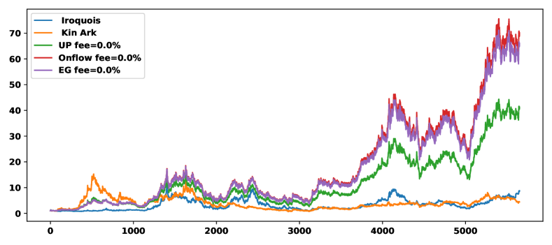
Figure 1: Results for the pair ’Irocquois’ – ’Kin Ark’, fee level=$0\%$: evolution of the UP, EG and Onflow portfolios. EG and Onflow perform similarly, better than UP which at its turn is better than the individual assets.

A pair that is known to provide good performance (cf. [8]) is ’Irocquois’ and ’Kin Ark’ (figures 1 and 2). The individual stocks increase by a factor of $8.92$ and $4.13$ respectively, while UP obtains around $40$ times the initial wealth. Even more, EG and Onflow manage to obtain around $70$ times the initial wealth, which is a substantial improvement over UP (and individual stocks). Even if Onflow is slightly better, the difference does not seem to be substantial. On the other hand, when the fee level $\xi$ increases to $2\%$ the performance of all the portfolios except Onflow degrade to the point of not being superior to that of simple buy-and-hold strategies on individual stocks. This result is consistent with the literature, that witness of the severe impact of the transaction costs on dynamic portfolio strategies. Here the Onflow parameter $\tau$ was set to $1$.

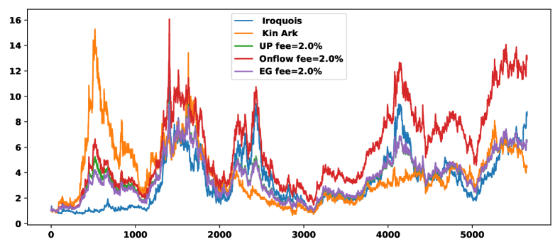
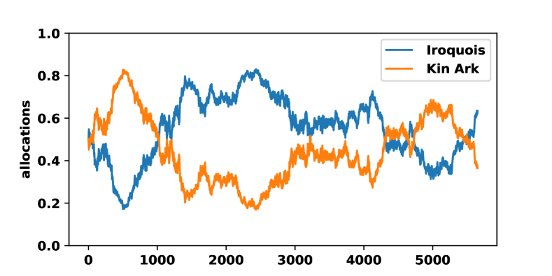
Figure 2: Results for the pair ’Irocquois’ – ’Kin Ark’, fee level=$2\%$. Top : evolution of the UP, EG and Onflow portfolio. With this fee level only the Onflow portfolio performs better than the individual assets. Bottom : the allocations of the Onflow portfolio.

The cumulative turnover (often called "rotation rate" in fund prospectus) is plotted in figure 3; when $\xi=0$ the daily portfolio turnover $\sum_{k}|\pi_{t+}-\pi_{t}|$ (mean relative transaction volume) is around $2\%$ for all strategies UP, EG and Onflow ; when $\xi=2\%$ UP and EG keep the turnover at the same level while Onflow reduces it to $0.5\%$. This explains the performance of Onflow in this case. Note that a level of daily turnover of $2\%$ corresponds to over $500\%$ annual turnover while $0.5\%$ means about $125\%$ annually. Over the whole period of $22$ years, UP and EG have a turnover of around $100$ times the portfolio value while Onflow has a total turnover $\sim 25$.

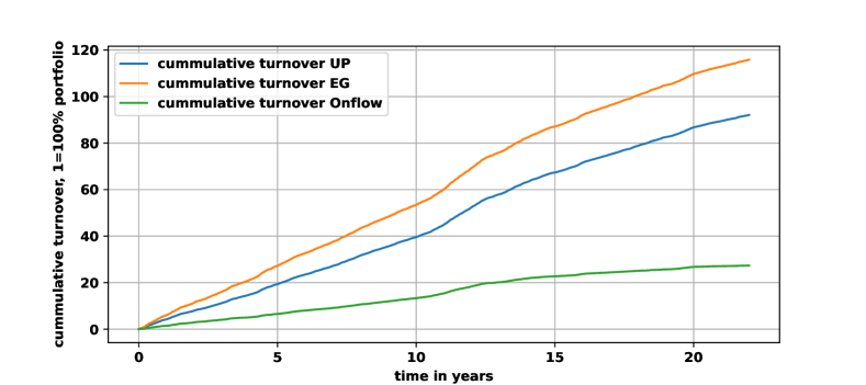
Figure 3: Cumulative turnover for the pair ’Irocquois’ – ’Kin Ark’, fee level=$2\%$: Units are set such that a value of $1$ corresponds to a $100\%$ portfolio turnover. For instance the total turnover over the whole period for UP is around $90$ times the portfolio value (not to be mistaken with $90\%$!).

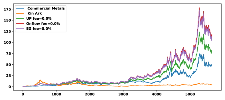
Figure 4: Same results as in figure 1 for the pair ’Commercial Metals’ – ’Kin Ark’, $\xi=0\%$.

Our second test is the pair ’Commercial Metals’ – ’Kin Ark’ (figures 4-5). Same general conclusions hold here, with performance of individual stocks not exceeding $50$ times initial wealth, Cover UP being above this at around $80$ while EG and Onflow are above UP at around $110$ when $\xi=0$. When $\xi=2\%$ the performance deteriorates : UP and EG decrease to $\sim 15$ while Onflow manages to retain cca. $50$ times initial wealth. In this case the reason is simple : in hindsight the ’Commercial Metals’ has a very impressive performance over the period and the best thing to do it is to passively follow it. This is what the Onflow algorithm manages to do as one can see in the bottom plot of figure 5 which shows that past the time $1000$ the allocation of "Commercial Metals" is always superior to that of ’Kin Ark’ and goes often as high as $80\%$ of the overall portfolio.

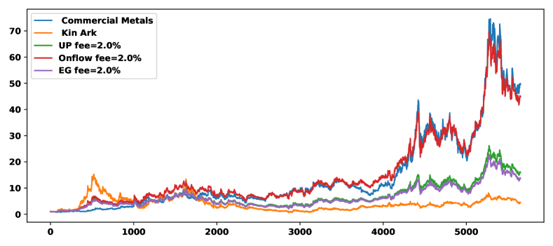
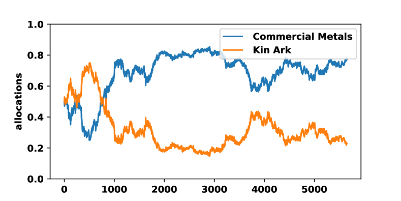
Figure 5: Same results as in figure 2 for the pair ’Commercial Metals’ – ’Kin Ark’, $\xi=2\%$.

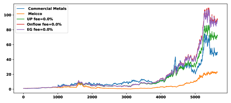
Figure 6: Same results as in figure 1 for the pair ’Commercial Metals’ – ’Meicco’, $\xi=0\%$.

The results for pair ’Commercial Metals’ – ’Meicco’, are presented in figures 6 and 7. As before, the impressive performance of the ’Commercial Metals’ stock does not allow for much improvement, with the Onflow algorithm remaining competitive even when fees are taken into account.

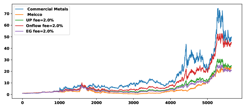
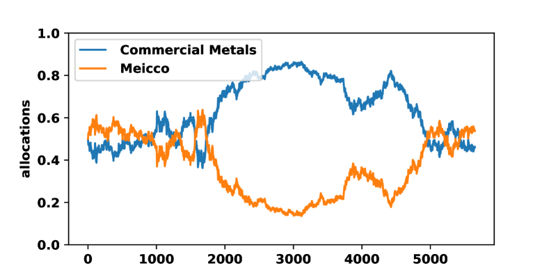
Figure 7: Same results as in figure 2 for the pair ’Commercial Metals’ – ’Meicco’, $\xi=2\%$.

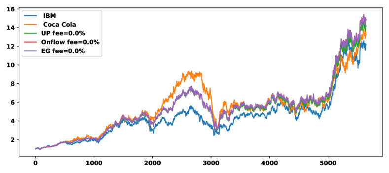
Figure 8: Same results as in figure 1 for the pair ’IBM’ – ’Coca Cola’, $\xi=0\%$.

Finally, we consider a situation where dynamic portfolios do not work well, the pair ’IBM’ – ’Coca Cola’. Without transaction costs all portfolios are comparable to individual assets. However at $2\%$ fee level UP and EG are not as good as the individual stocks while Onflow manages to obtain comparable results.

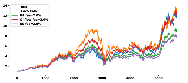
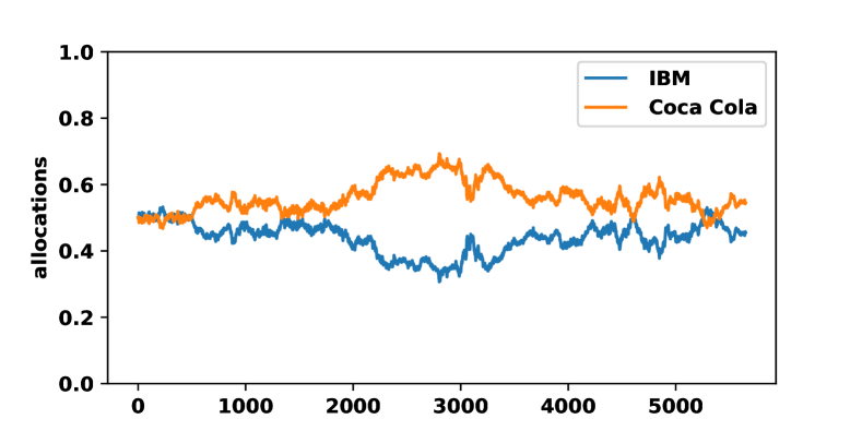
Figure 9: Same results as in figure 2 for the pair ’IBM’ – ’Coca Cola’, $\xi=2\%$.

5 Conclusion

We introduce in this paper OnFlow, an online portfolio allocation algorithm. It works without any assumption on the statistics of the asset price time series by repeatedly adjusting the portfolio allocation according to new market data in a reinforcement learning style. Onflow uses a softmax representation of the allocation and solves during each time step a gradient flow evolution equation that can be implemented through a simple ODE; this gradient flow also contains terms to minimize the transaction costs.

For the case of log-normal continuous time evolution and assuming that true gradients can be used, we show theoretically under some technical assumptions that the procedure will converge to the optimum allocation.

The empirical performance of the procedure was tested on some standard benchmarks with satisfactory results. When compared to classic strategies such as the Universal Portfolio of Cover or the EG algorithm from [12] it provides a comparable (even slightly better) performance when transactions fees are zero and performs generally significantly better when severe transactions fees of up to $2\%$ are considered (a level that previous algorithms did not treat very well).

Some extensions of this work are investigated by the authors to add the possibility of short positions (see also remark 3) and to test for other markets and different periods.

6 Ethical Statement

The authors do not declare any conflicts of interests. The research did not involve any human subjects and/or animals subjects.

References

- \bibcommenthead
- Agarwal \BOthers. [\APACyear2021] \APACinsertmetastaragarwal_theory_2021_cv_policy_grad{APACrefauthors}Agarwal, A., Kakade, S.M., Lee, J.D.\BCBL Mahajan, G. \APACrefYearMonthDay2021. \BBOQ\APACrefatitleOn the Theory of Policy Gradient Methods: Optimality, Approximation, and Distribution Shift On the Theory of Policy Gradient Methods: Optimality, Approximation, and Distribution Shift.\BBCQ \APACjournalVolNumPagesJournal of Machine Learning Research22981–76, {APACrefURL} http://jmlr.org/papers/v22/19-736.html \PrintBackRefs\CurrentBib
- Amari [\APACyear1998] \APACinsertmetastaramari_natural_gradient_98{APACrefauthors}Amari, S\BHBIi. \APACrefYearMonthDay1998. \BBOQ\APACrefatitleNatural Gradient Works Efficiently in Learning Natural gradient works efficiently in learning.\BBCQ \APACjournalVolNumPagesNeural Computation102251-276, {APACrefDOI} https://doi.org/10.1162/089976698300017746 \PrintBackRefs\CurrentBib
- Black \BBA Litterman [\APACyear1990] \APACinsertmetastarblack1990asset{APACrefauthors}Black, F.\BCBT \BBA Litterman, R. \APACrefYearMonthDay1990. \BBOQ\APACrefatitleAsset allocation: combining investor views with market equilibrium Asset allocation: combining investor views with market equilibrium.\BBCQ \APACjournalVolNumPagesGoldman Sachs Fixed Income Research11517–18, \PrintBackRefs\CurrentBib
- Blum \BBA Kalai [\APACyear1997] \APACinsertmetastarblum1997universal{APACrefauthors}Blum, A.\BCBT \BBA Kalai, A. \APACrefYearMonthDay1997. \BBOQ\APACrefatitleUniversal portfolios with and without transaction costs Universal portfolios with and without transaction costs.\BBCQ \APACrefbtitleProceedings of the Tenth Annual Conference on Computational Learning Theory Proceedings of the tenth annual conference on computational learning theory (\BPGS 309–313). \PrintBackRefs\CurrentBib
- Borodin \BOthers. [\APACyear2003] \APACinsertmetastarborodin2003can{APACrefauthors}Borodin, A., El-Yaniv, R.\BCBL Gogan, V. \APACrefYearMonthDay2003. \BBOQ\APACrefatitleCan we learn to beat the best stock Can we learn to beat the best stock.\BBCQ \APACjournalVolNumPagesAdvances in Neural Information Processing Systems16, \PrintBackRefs\CurrentBib
- Cesa-Bianchi \BBA Lugosi [\APACyear2006] \APACinsertmetastarcesa2006prediction{APACrefauthors}Cesa-Bianchi, N.\BCBT \BBA Lugosi, G. \APACrefYear2006. \APACrefbtitlePrediction, learning, and games Prediction, learning, and games. \APACaddressPublisherCambridge university press. \PrintBackRefs\CurrentBib
- Charbonnier \BOthers. [\APACyear1997] \APACinsertmetastarpseudo_huber_loss{APACrefauthors}Charbonnier, P., Blanc-Feraud, L., Aubert, G.\BCBL Barlaud, M. \APACrefYearMonthDay1997feb. \BBOQ\APACrefatitleDeterministic Edge-Preserving Regularization in Computed Imaging Deterministic edge-preserving regularization in computed imaging.\BBCQ \APACjournalVolNumPagesTrans. Img. Proc.62298–311, {APACrefDOI} https://doi.org/10.1109/83.551699 {APACrefURL} https://doi.org/10.1109/83.551699 \PrintBackRefs\CurrentBib
- Cover [\APACyear1991] \APACinsertmetastarcover91{APACrefauthors}Cover, T.M. \APACrefYearMonthDay1991. \BBOQ\APACrefatitleUniversal Portfolios Universal portfolios.\BBCQ \APACjournalVolNumPagesMathematical Finance111-29, {APACrefDOI} https://doi.org/https://doi.org/10.1111/j.1467-9965.1991.tb00002.x {APACrefURL} https://onlinelibrary.wiley.com/doi/abs/10.1111/j.1467-9965.1991.tb00002.x https://onlinelibrary.wiley.com/doi/pdf/10.1111/j.1467-9965.1991.tb00002.x \PrintBackRefs\CurrentBib
- Dochow [\APACyear2016] \APACinsertmetastardochow_proposed_2016{APACrefauthors}Dochow, R. \APACrefYearMonthDay2016. \BBOQ\APACrefatitleProposed Algorithms with Risk Management Proposed Algorithms with Risk Management.\BBCQ \APACrefbtitleOnline Algorithms for the Portfolio Selection Problem Online Algorithms for the Portfolio Selection Problem (\BPGS 109–126). \APACaddressPublisherWiesbadenSpringer Fachmedien Wiesbaden. {APACrefURL} https://doi.org/10.1007/978-3-658-13528-7_5 \PrintBackRefs\CurrentBib
- Györfi \BOthers. [\APACyear2012] \APACinsertmetastarbook_fin_rl12{APACrefauthors}Györfi, L., Ottucsák, G.\BCBL Walk, H. \APACrefYear2012. \APACrefbtitleMachine Learning for Financial Engineering Machine learning for financial engineering. \APACaddressPublisherIMPERIAL COLLEGE PRESS. {APACrefURL} https://www.worldscientific.com/doi/abs/10.1142/p818 \PrintBackRefs\CurrentBib
- He \BBA Li [\APACyear2023] \APACinsertmetastarhe_new_2023{APACrefauthors}He, H.\BCBT \BBA Li, H. \APACrefYearMonthDay2023\APACmonth04. \BBOQ\APACrefatitleA New Boosting Algorithm for Online Portfolio Selection Based on dynamic Time Warping and Anti-correlation A New Boosting Algorithm for Online Portfolio Selection Based on dynamic Time Warping and Anti-correlation.\BBCQ \APACjournalVolNumPagesComputational Economics, {APACrefDOI} https://doi.org/10.1007/s10614-023-10383-6 {APACrefURL} https://doi.org/10.1007/s10614-023-10383-6 \PrintBackRefs\CurrentBib
- Helmbold \BOthers. [\APACyear1998] \APACinsertmetastarHelmbold98{APACrefauthors}Helmbold, D.P., Schapire, R.E., Singer, Y.\BCBL Warmuth, M.K. \APACrefYearMonthDay1998. \BBOQ\APACrefatitleOn-Line Portfolio Selection Using Multiplicative Updates On-line portfolio selection using multiplicative updates.\BBCQ \APACjournalVolNumPagesMathematical Finance84325-347, {APACrefDOI} https://doi.org/https://doi.org/10.1111/1467-9965.00058 {APACrefURL} https://onlinelibrary.wiley.com/doi/abs/10.1111/1467-9965.00058 https://onlinelibrary.wiley.com/doi/pdf/10.1111/1467-9965.00058 \PrintBackRefs\CurrentBib
- Jamshidian [\APACyear1992] \APACinsertmetastarcont_time_univ_portf_jamshidian92{APACrefauthors}Jamshidian, F. \APACrefYearMonthDay1992. \BBOQ\APACrefatitleASYMPTOTICALLY OPTIMAL PORTFOLIOS Asymptotically optimal portfolios.\BBCQ \APACjournalVolNumPagesMathematical Finance22131-150, {APACrefDOI} https://doi.org/https://doi.org/10.1111/j.1467-9965.1992.tb00042.x {APACrefURL} https://onlinelibrary.wiley.com/doi/abs/10.1111/j.1467-9965.1992.tb00042.x https://onlinelibrary.wiley.com/doi/pdf/10.1111/j.1467-9965.1992.tb00042.x \PrintBackRefs\CurrentBib
- Jordan \BOthers. [\APACyear1998] \APACinsertmetastarjko{APACrefauthors}Jordan, R., Kinderlehrer, D.\BCBL Otto, F. \APACrefYearMonthDay1998. \BBOQ\APACrefatitleThe variational formulation of the Fokker-Planck equation The variational formulation of the Fokker-Planck equation.\BBCQ \APACjournalVolNumPagesSIAM J. Math. Anal.2911–17, {APACrefDOI} https://doi.org/10.1137/S0036141096303359 {APACrefURL} http://dx.doi.org/10.1137/S0036141096303359 \PrintBackRefs\CurrentBib
- Kalai \BBA Vempala [\APACyear2002] \APACinsertmetastarkalai2002efficient{APACrefauthors}Kalai, A.T.\BCBT \BBA Vempala, S. \APACrefYearMonthDay2002. \BBOQ\APACrefatitleEfficient algorithms for universal portfolios Efficient algorithms for universal portfolios.\BBCQ \APACjournalVolNumPagesJournal of Machine Learning Research423–440, \PrintBackRefs\CurrentBib
- Kelly Jr [\APACyear1956] \APACinsertmetastarkelly1956new{APACrefauthors}Kelly Jr, J.L. \APACrefYearMonthDay1956. \BBOQ\APACrefatitleA New Interpretation of Information Rate A new interpretation of information rate.\BBCQ \APACjournalVolNumPagesBell System Technical Journal354917–926, {APACrefDOI} https://doi.org/10.1002/j.1538-7305.1956.tb03809.x \PrintBackRefs\CurrentBib
- Kempf \BBA Memmel [\APACyear2006] \APACinsertmetastarkempf_estim_min_var_2006{APACrefauthors}Kempf, A.\BCBT \BBA Memmel, C. \APACrefYearMonthDay2006\APACmonth10. \BBOQ\APACrefatitleEstimating the Global Minimum Variance Portfolio Estimating the Global Minimum Variance Portfolio.\BBCQ \APACjournalVolNumPagesSchmalenbach Business Review584332–348, {APACrefDOI} https://doi.org/10.1007/BF03396737 {APACrefURL} https://doi.org/10.1007/BF03396737 \PrintBackRefs\CurrentBib
- Li \BBA Hoi [\APACyear2014] \APACinsertmetastarli2014online_survey{APACrefauthors}Li, B.\BCBT \BBA Hoi, S.C. \APACrefYearMonthDay2014. \BBOQ\APACrefatitleOnline portfolio selection: A survey Online portfolio selection: A survey.\BBCQ \APACjournalVolNumPagesACM Computing Surveys (CSUR)4631–36, \PrintBackRefs\CurrentBib
- Li \BOthers. [\APACyear2015] \APACinsertmetastarli_moving_avg_portf_2015{APACrefauthors}Li, B., Hoi, S.C.H., Sahoo, D.\BCBL Liu, Z\BHBIY. \APACrefYearMonthDay2015. \BBOQ\APACrefatitleMoving average reversion strategy for on-line portfolio selection Moving average reversion strategy for on-line portfolio selection.\BBCQ \APACjournalVolNumPagesArtificial Intelligence222104–123, {APACrefDOI} https://doi.org/https://doi.org/10.1016/j.artint.2015.01.006 {APACrefURL} https://www.sciencedirect.com/science/article/pii/S0004370215000168 \PrintBackRefs\CurrentBib
- Li \BOthers. [\APACyear2016] \APACinsertmetastarli2016olps{APACrefauthors}Li, B., Sahoo, D.\BCBL Hoi, S.C. \APACrefYearMonthDay2016. \BBOQ\APACrefatitleOLPS: a toolbox for on-line portfolio selection Olps: a toolbox for on-line portfolio selection.\BBCQ \APACjournalVolNumPagesThe Journal of Machine Learning Research1711242–1246, \PrintBackRefs\CurrentBib
- Marigold [\APACyear2013] \APACinsertmetastarmarigold_github_up{APACrefauthors}Marigold \APACrefYearMonthDay2013. \BBOQ\APACrefatitleUniversal Portfolios Universal portfolios.\BBCQ \APACjournalVolNumPagesGitHub repository, \APACrefnoteretrieved 01/11/2023 \PrintBackRefs\CurrentBib
- Markowitz [\APACyear1952] \APACinsertmetastarmarkovitz_portfolio_theory{APACrefauthors}Markowitz, H. \APACrefYearMonthDay1952. \BBOQ\APACrefatitlePortfolio Selection Portfolio selection.\BBCQ \APACjournalVolNumPagesThe Journal of Finance7177–91, {APACrefURL} [2023-11-24]http://www.jstor.org/stable/2975974 \PrintBackRefs\CurrentBib
- Mei \BOthers. [\APACyear2020] \APACinsertmetastarmei20_cv_softmax_policy{APACrefauthors}Mei, J., Xiao, C., Szepesvari, C.\BCBL Schuurmans, D. \APACrefYearMonthDay202013–18 Jul. \BBOQ\APACrefatitleOn the Global Convergence Rates of Softmax Policy Gradient Methods On the global convergence rates of softmax policy gradient methods.\BBCQ H.D. III \BBA A. Singh (\BEDS), \APACrefbtitleProceedings of the 37th International Conference on Machine Learning Proceedings of the 37th international conference on machine learning (\BVOL 119, \BPGS 6820–6829). \APACaddressPublisherPMLR. {APACrefURL} https://proceedings.mlr.press/v119/mei20b.html \PrintBackRefs\CurrentBib
- Robbins \BBA Monro [\APACyear1951] \APACinsertmetastarrobbins_stochastic_1951{APACrefauthors}Robbins, H.\BCBT \BBA Monro, S. \APACrefYearMonthDay1951. \BBOQ\APACrefatitleA Stochastic Approximation Method A Stochastic Approximation Method.\BBCQ \APACjournalVolNumPagesThe Annals of Mathematical Statistics223400 – 407, {APACrefDOI} https://doi.org/10.1214/aoms/1177729586 {APACrefURL} https://doi.org/10.1214/aoms/1177729586 \APACrefnotePublisher: Institute of Mathematical Statistics \PrintBackRefs\CurrentBib
- Sutton \BBA Barto [\APACyear2018] \APACinsertmetastarsutton_reinforcement_2018{APACrefauthors}Sutton, R.S.\BCBT \BBA Barto, A.G. \APACrefYear2018. \APACrefbtitleReinforcement learning. An introduction Reinforcement learning. An introduction (\PrintOrdinal2nd expanded and updated edition \BEd). \APACaddressPublisherCambridge, MA: MIT Press. \PrintBackRefs\CurrentBib
- Turinici [\APACyear2021] \APACinsertmetastarturinici_radonsobolev_2021{APACrefauthors}Turinici, G. \APACrefYearMonthDay2021. \BBOQ\APACrefatitleRadon–Sobolev Variational Auto-Encoders Radon–Sobolev Variational Auto-Encoders.\BBCQ \APACjournalVolNumPagesNeural Networks141294–305, {APACrefDOI} https://doi.org/10.1016/j.neunet.2021.04.018 \PrintBackRefs\CurrentBib
- Turinici [\APACyear2023] \APACinsertmetastargabriel_turinici_convergence_2023{APACrefauthors}Turinici, G. \APACrefYearMonthDay2023. \APACrefbtitleThe convergence of the Stochastic Gradient Descent (SGD) : a self-contained proof. The convergence of the Stochastic Gradient Descent (SGD) : a self-contained proof. \APACaddressPublisherZenodo. {APACrefURL} https://zenodo.org/doi/10.5281/zenodo.4638694 \PrintBackRefs\CurrentBib