Minimax dual control with finite-dimensional information state

Abstract

This article considers output-feedback control of systems where the function mapping states to measurements has a set-valued inverse. We show that if the set has a bounded number of elements, then minimax dual control of such systems admits finite-dimensional information states. We specialize our results to a discrete-time integrator with magnitude measurements and derive a surprisingly simple sub-optimal control policy that ensures finite gain of the closed loop. The sub-optimal policy is a proportional controller where the magnitude of the gain is computed offline, but the sign is learned, forgotten, and relearned online.

The discrete-time integrator with magnitude measurements captures real-world applications such as antenna alignment, and despite its simplicity, it defies established control-design methods. For example, whether a stabilizing linear time-invariant controller exists for this system is unknown, and we conjecture that none exists.

1 Introduction

This article concerns the ouput feedback control of discrete-time systems whose measurement equations have a bounded number of solutions. As a prototype example, we consider the discrete-time integrator, where the controller only has access to the magnitude of the state. The state $x_{t}$, control signal $u_{t}$, and disturbance $w_{t}$ are real-valued scalars. The system is described by the recursion

$$x_{t+1}=x_{t}+u_{t}+w_{t}.$$ (1)

We consider causal control policies, $\mu$, that map measurements of the state magnitude

$$y_{t}=|x_{t}|$$ (2)

to control signals

$$u_{t}=\mu_{t}(y_{0},y_{1},\ldots,y_{t},u_{0},\ldots,u_{t-1}).$$ (3)

The uncertain sign in (2) captures some of the difficulties that may arise when optimizing a system based on measurements of some (locally) convex or concave performance quantity, as in Figure 1. The problem is also closely related to stabilizing an inverted pendulum by feedback from height measurements rather than angular measurements, as in Figure 1.

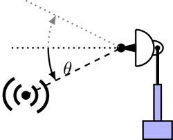
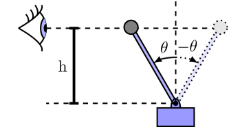
Figure 1: Examples of physical systems where the sign of the state is ambiguous: The left figure depicts a receiver whose source location is unknown and possibly non-stationary. The goal is to steer the receiver to an angle where the signal intensity is maximized. The radiant sensitivity of the receiver is typically symmetric in the deviation from the incidence angle. The right figure depicts an inverted pendulum controlled by measuring the height of the pendulum.

This plain-looking problem captures a surprising amount of complexity:

1. Exploration vs. exploitation. The better we control the system, the less we can say about the sign of the state; if we ever reach $y=0$, then all knowledge about the sign of the state is lost.

2. No stabilizing linear time-invariant controller. Previous work report no stabilizing linear time-invariant controller for the system (1)–(3) Rosdahl and Bernhardsson (2020); Alspach (1972) and the system cannot be stabilized by proportional feedback. This author conjectures that there exists no finite-dimensional linear time-invariant controller that stabilizes the system.

3. Extended Kalman filter. The extended Kalman filter (EKF) is a popular algorithm for estimating the state of a nonlinear system, and is often coupled with certainty-equivalence control. However, the measurement equation (2) is not differentiable at $x=0$, and the EKF is not directly applicable. One may substitute the measurement equation with $y_{t}=x_{t}^{2}$ to recover differentiability, but this substitution renders the linearization unobservable.

4. Myopic Controller. The Myopic controller Wittenmark (1995) associated with minimizing the current cost $x_{t}^{2}+u_{t}^{2}$ is not stabilizing.

In this article, we will design a control policy (3) that ensures that the induced $\ell_{2}$-gain from $w$ to $(x,u)$ is less than some positive quantity $\gamma$. That is, the inequality

$$\sum_{t=0}^{N}(x_{t}^{2}+u_{t}^{2})\leq\gamma^{2}\sum_{t=0}^{N}w_{t}^{2}+\beta(x_{0})$$ (4)

must be fulfilled for all $N\geq 0$, real-valued function $\beta$ and realizations $w_{0:N}:=w_{0},w_{1},\ldots,w_{N}$ of the disturbance sequence. The condition (4) generalizes the classical $\mathcal{H}_{\infty}$-norm for linear systems. The function $\beta$ is called a bias term and is used to capture the effect of the initial state. Together with the small-gain theorem it provides sufficient conditions for robust stability against feedback perturbations with induced $\ell_{2}$-norm less than $\gamma^{-1}$. We refer the reader to (Khalil, 2002, Chapter 5) for a detailed discussion on finite-gain stability and the small-gain theorem. Surprisingly, we will see that it is possible to compress the observed output trajectory $(y_{0:t},u_{0:t-1})$ using two recursively computed quantities $r^{+}_{t}$ and $r^{-}_{t}$. These quantities correspond to the smallest feasible disturbance trajectory compatible with the observed outputs and $\operatorname{sign}(x_{t})=1$ or $\operatorname{sign}(x_{t})=-1$. Together with $y_{t}$, they make a sufficient statistic for optimal control of a corresponding dynamic game. The quantities follow the recursions

$$r^{+}_{t+1} =y_{t}^{2}+u_{t}^{2}-\gamma^{2}\max\{r^{+}_{t}+(y_{t+1}-u_{t}-y_{t})^{2},r^{-}_{t}+\gamma^{2}(y_{t+1}-u_{t}+y_{t})^{2}\},$$ (5)

$$r^{-}_{t+1} =y_{t}^{2}+u_{t}^{2}-\gamma^{2}\max\{r^{+}_{t}+(-y_{t+1}-u_{t}-y_{t})^{2},r^{-}_{t}+(-y_{t+1}-u_{t}+y_{t})^{2}\}.$$

We will show in Section 3 that Theorem 5 implies that this compression is lossless:

Proposition 1.

There exists an admissible policy $\mu$ that ensures an $\ell_{2}$-gain smaller than $\gamma$ if, and only if, it can be achieved with a policy of the form

$$u_{t}=\eta_{t}(y_{t},r^{+}_{t},r^{-}_{t}).$$ (6)

We also use Theorem 6 to construct a controller that ensures that the $\ell_{2}$-gain is less than $4$:

Proposition 2.

The controller

$$\eta(y,r^{+},r^{-})=\begin{cases}-0.7y,&\text{if }r^{+}\leq r^{-},\\ 0.7y,&\text{if }r^{+}>r^{-}\end{cases}$$ (7)

achieves $\ell_{2}$-gain less than $4$.

We remark that $\eta$ is admissible as $r^{+}_{t}$ and $r^{-}_{t}$ are functions of $y_{0:t}$ and $u_{0:t-1}$. Via substitution, one can recover $\mu$.

1.1 Related work

Adaptive control

From the adaptive control perspective, system (1), (2) could be interpreted as a linear system with uncertain time-varying parameters. Several methods described in excellent textbooks like (Goodwin and Sin, 2009, Chapter 6.7) that apply uncertain linear time-varying systems. However, these methods rely on a separation of time scales between the dynamics of the state, the parameter adaptation, and the parameter variation. Hence, we can not expect these methods to work well in our case Anderson and Dehghani (2008). Nonlinear stochastic control theory provides a framework that can, in principle, handle fast parameter variation and large uncertainties, and our problem fits well with the methodology of dual control (Wittenmark, 1995, Chapter 7).

Stochastic dual control has been applied to various problems where the gain is uncertain, e.g., Åström and Helmersson (1986); Dumont and Åström (1988); Allison et al. (1995). Alspach (1972) considered control of an integrator based on noisy measurements of the square of the magnitude. The noise was assumed Gaussian, and the author proposed approximating the information state by a sum of Gaussians. Rosdahl and Bernhardsson (2020) considered a noisy version of the problem in this article but from a stochastic dual control perspective. The authors proposed to approximate the information state by a neural network.

Learning-to-control

Lately, there has been a surge of interest in learning to control linear systems. Much of the work concerns the sample complexity of learning optimal controllers of linear time-invariant systems. For example, Dean et al. (2018); Mania et al. (2019) concerns quadratic performance objectives and additive stochastic noise, Chen and Hazan (2021) adapts the theory of online convex optimization Hazan (2023) to unknown linear time-invariant systems with bounded disturbances. Yu et al. (2023) proposed a method to control slowly varying linear systems with unknown parameters belonging to a polytope perturbed by bounded disturbances. Their controller is based on convex body chasing.

Minimax control

Minimax control for uncertain systems was introduced in the Ph.D. thesis of Witsenhausen (1966). Information states, or sufficient statistics, for optimal control for output feedback minimax control was discussed in Bertsekas and Rhodes (1973) based on Bertsekas’s Ph.D. thesis. The game-theoretic formulation of $\mathcal{H}_{\infty}$-control Baş̧ar and Bernhard (2008) is a special case of minimax control, and the information state formulation was rederived for nonlinear systems in James and Baras (1995) where it is shown that, in general, the information state is infinite-dimensional. The term minimax adaptive control was introduced in Didinsky and Basar (1994). Recently, Rantzer (2021) proposed a minimax adaptive controller for uncertain linear systems with perfect state measurements. The uncertainty was assumed to belong to a finite, known set. The author proposed a finite-dimensional information state related to the empirical covariance matrix of the current state, previous state and previous control signal. This author extended Rantzer’s results to scalar linear systems with noisy measurements in Kjellqvist and Rantzer (2022). Recently, Renganathan et al. (2023) studied the regret of Rantzer’s controller for linear systems with energy-bounded disturbances.

1.2 Contributions

This article identifies a class of systems where the minimax dual controller admits a finite-dimensional information state. The information state admits recursive computation, and Theorem 5 shows the equivalence between the minimax dual control problem and an information-state dynamic programming problem. We also provide a dissipativity interpretation in Theorem 6. These results can be seen as generalizations of Theorem 1 in Rantzer (2021) or a specialization of the results in James and Baras (1995). We specialize these results to the magnitude control problem in the introduction and prove that the $\ell_{2}$-gain is less than $4$ for the controller $\eta$ in (7).

1.3 Notation

We use $\mathbb{R}$ to denote the set of real numbers, $\mathbb{R}^{n}$ means the set of $n$-dimensional real vectors, and $\mathbb{R}^{n\times m}$ to denotes the set of $n\times m$ real matrices. For vectors $v,v^{\prime}\in\mathbb{R}^{n}$, the inequality $v\leq v^{\prime}$ is understood component-wise. The vector of ones is denoted $\mathbf{1}$. We use $y_{0:N}$ as shorthand for the sequence $(y_{0},y_{1},\ldots,y_{N})$. For a matrix $A\in\mathbb{R}^{n\times m}$, we denote the transpose by $A^{\mkern-1.5mu\mathsf{T}}$. For a set $S$, the preimage under function $f$ is denoted $f^{-1}(S)$. For two sets $S$ and $T$, the Cartesian product is denoted $S\times T$ and the $n$-ary Cartesian power is denoted $S^{n}$.

2 Minimax dual control

This section introduces the minimax dual control problem, the information state and dynamic programming. It is well known that the “worst-case” history is an information state for the minimax control problem and dynamic programming with respect to this information state is fairly well understood. Unfortunately, this information state is, in general, infinite dimensional and therefore impractical. The main contribution of this section is to show that for our class of systems, the worst-case history admits a finite-dimensional representation. This representation is, in itself, an information state. We rederive a verification and an approximation theorem for value iteration with respect to this finite-dimensional representation.

2.1 Problem formulation

Let $f:\mathcal{X}\times\mathcal{U}\times\mathcal{W}\to\mathcal{X}$ and $h:\mathcal{X}\to\mathcal{Y}$ describe the dynamical system

$$x_{t+1} =f(x_{t},u_{t},w_{t})$$ (8)

$$y_{t} =h(x_{t}).$$

The control signal, $u_{t}\in\mathcal{U}$ is generated by a causal control policy $\mu_{t}:\mathcal{Y}^{t}\times\mathcal{U}^{t-1}\to\mathcal{U}$, where $\mathcal{Y}=h(\mathcal{X})$ by

$$u_{t}=\mu_{t}(y_{0:t},u_{0:t-1}).$$ (9)

We call the tuple $\pi=(\mu_{0},\mu_{1},\ldots)$ a strategy and the set of all such admissible strategies $\Pi$. Consider the objective function as the “worst-case” sum of stage costs $l:\mathcal{X}\times\mathcal{U}\times\mathcal{W}\to\mathbb{R}$,

$$J_{\pi}^{N}(x_{0})\triangleq\sup_{w_{0:N}\in\mathcal{W}^{N+1}}\sum_{t=0}^{N}l(x_{t},u_{t},w_{t}).$$ (10)

The goal of this section is to examine the minimax optimal control problem

$$J_{\star}(x_{0})\triangleq\inf_{\pi\in\Pi}\sup_{N}J_{\pi}^{N}(x_{0}).$$ (11)

We make two crucial assumptions:

Assumption 1.

For all $x\in\mathcal{X},u\in\mathcal{U}$, $\sup_{w}l(x,u,w)\geq 0$ and for all $x\in\mathcal{X},w\in\mathcal{W}$, $\inf_{u}l(x,u,w)>-\infty$.

The assumption that $\inf_{u}l(x,u,w)>-\infty$ allows us to use standard arguments for dynamic programming, and the assumption that $\sup_{w}l(x,u,w)\geq 0$ implies monotonicity properties of $J_{\pi}^{N}$ in (10) and, as we will see later, the value iteration.

Proposition 1 (Monotonicity of $J_{\pi}^{N}$).

For any strategy $\pi$, $J_{\pi}^{N}(x_{0})$ is nondecreasing in $N$.

Assumption 2.

For any $y\in\mathcal{Y}$, the set $h^{-1}\{x\}$ has at most $M$ elements.

This assumption relates to the dimensionality of the information state, or sufficient statistic, of the dynamic programming version of this problem. Technically, the bound $M$ does not have to be known a priori, but we require the capability to enumerate all the solutions to $y_{t}=h(x_{t})$ online. Although this assumption may seem highly restrictive, we can increase the applicability by storing past values of the measurements.

Remark 3.

In our case $f$ and $h$ are given by (1) and (2) and the stage cost is $l(x_{t},u_{t},w_{t})=x_{t}^{2}+u_{t}^{2}-\gamma^{2}w_{t}^{2}$. The states, observations and inputs take values in $\mathcal{X}=\mathbb{R},\mathcal{U}=\mathbb{R},\mathcal{Y}=\mathbb{R}_{\geq 0},\mathcal{W}=\mathbb{R}$. The finite-gain condition (4) then correspond to $J_{\star}(x_{0})$ being bounded. If not for the nonlinearity $h(x_{t})=|x_{t}|$, it would be equivalent to the standard dynamic game formulation of $\mathcal{H}_{\infty}$ suboptimal control Baş̧ar and Bernhard (2008), rather it can be seen as a special case of nonlinear $\mathcal{H}_{\infty}$ output feedback control James and Baras (1995).

2.2 An information state

Following previous work Witsenhausen (1966); Bertsekas and Rhodes (1973); James and Baras (1995); Baş̧ar and Bernhard (2008) we consider the “worst-case history”, $\rho_{t}$, that is compatible with the observations $y_{0:t-1}$ and inputs $u_{0:t-1}$ up to time $t-1$:

$$\rho_{t}(x,y_{0:t-1},u_{0:t-1})\\ \triangleq\sup_{w_{0:t-1}\in\mathcal{W}^{t-1}}\sup_{x_{0}\in\mathcal{X}}\left\{\sum_{\tau=0}^{t-1}l(x_{\tau},u_{\tau},w_{\tau}):x_{t}=x,x_{\tau+1}=f(x_{\tau},u_{\tau},y_{\tau}),y_{\tau}=h(x_{\tau})\right\}.$$ (12)

Remark 4.

We follow the convention that the supremum over the empty set is $-\infty$.

The worst-case performance given a policy $\pi\in\Pi$, $J_{\pi}^{N}(x_{0})$, can then be expressed in terms of the worst-case history $\rho_{t}$ as

$$J_{\pi}^{N}(x_{0})=\sup_{y_{0:N},x}\rho_{N+1}(x,y_{0:N},u_{0:N}),$$ (13)

where $u_{0:N}$ is generated by $\pi$ and $y_{0:N}$. We now derive a recursive expression for $\rho_{t}$ in terms of an $M$-dimensional vector. Let $\mathbf{r}_{t}=\begin{bmatrix}r_{t}^{1}&\cdots&r_{t}^{M}\end{bmatrix}^{\mkern-1.5mu\mathsf{T}}$ and define the function $g_{r}:(\mathbf{r}_{t-1},y_{t},y_{t-1},u_{t-1})\mapsto\mathbf{r}_{t}$ through its components by

$$\xi_{\tau}^{1},\ldots,\xi_{\tau}^{M} =h^{-1}\{y_{\tau}\},\qquad\tau=t,t-1$$ (14)

$$r_{t}^{i} =\sup_{j,w\in\mathcal{W}}\left\{l(\xi_{t-1}^{j},u_{t-1},w)+r_{t-1}^{j}:\xi_{t}^{i}=f(\xi_{t-1}^{j},u_{t-1},w),j\in 1,\ldots,M,w\in\mathcal{W}\right\}.$$

Proposition 2.

Fix $N$, $i=1,\ldots,M$, $y_{0}$, a strategy $\pi$ and let $\mathbf{r}_{N}$ be defined recursively by $\mathbf{r}_{0}=0$ and $\mathbf{r}_{t}=g_{r}(\mathbf{r}_{t-1},y_{t},y_{t-1},u_{t-1})$. Then the following hold:

1. There exists a sequence $v_{0:N-1}$ such that $\max_{i}r_{N}^{i}\geq 0$.

2. For fixed $y_{t},y_{t-1}\in\mathcal{Y}$ and $u_{t}\in\mathcal{U}$, for $\mathbf{r}\leq\mathbf{r}^{\prime}$ we have $g_{r}(\mathbf{r},y_{t},y_{t-1},u_{t})\leq g_{r}(\mathbf{r}^{\prime},y_{t},y_{t-1},u_{t})$.

3. $g_{r}(\mathbf{r}+\mathbf{1}c,y_{t},y_{t-1},u_{t})=g_{r}(\mathbf{r},y_{t},y_{t-1},u_{t})+\mathbf{1}c$ for all $c\in\mathbb{R}$.

4. $\rho_{t+1}(x,y_{0:t},u_{0:t})=\sup_{i,w}\left\{l(x,u_{t},w)+r_{t}^{i}:x=f(\xi_{t}^{i},u_{t},w)\right\}.$

Proof.

1. follows directly from Assumption 1. 2. follows from the monotonicity of the supremum operator. 3. follows from that for any function $f$ and set $Z$ $\sup_{z\in Z}\{f(z)+c\}=\sup_{x}\{f(z)\}+c$ for all $c\in\mathbb{R}$. 4 follows by recursion. ∎

2.3 Value iteration

Consider the time evolutions of the measurements $y$ and representations $\mathbf{r}$:

$$y_{t+1} =v_{t}$$ (15a)

$$\mathbf{r}_{t+1} =g_{r}(\mathbf{r}_{t},v_{t},y_{t},u_{t}),\quad\mathbf{r}_{0}=0,$$ (15b)

where $v_{t}$ is an exogenous input and $u_{t}$ is generated by an information-state feedback policy

$$u_{t}=\eta_{t}(\mathbf{r}_{t},y_{t}).$$

Define the set of information-state strategies $\widetilde{\Pi}$ as the set of strategies $\tilde{\pi}=(\eta_{0},\eta_{1},\ldots)$. As $\mathbf{r}$ is a causal function of the measurements and control signals, so is $\eta_{t}$ (by composition) and $\widetilde{\Pi}\subset\Pi$. In other words, information-state feedback is admissible.

Define the Bellman operators $\operatorname{\mathcal{B}}$ and $\operatorname{\mathcal{B}}_{u}$ by

$$\operatorname{\mathcal{B}}V(\mathbf{r},y)=\min_{u\in\mathcal{U}(y)}\overbrace{\max_{v\in\mathcal{Y}}\left\{V(g_{r}(\mathbf{r},v,y,u),v)\right\}}^{\operatorname{\mathcal{B}}_{u}V(\mathbf{r},y)}.$$ (16)

As both the minimum and the maximum operators are monotone, so are the Bellman operators:

Proposition 3 (Monotonicity of $\operatorname{\mathcal{B}}$).

For two functions $V$ and $V^{\prime}$ $:(\mathbb{R}\cup\{-\infty\})^{M}\times\mathcal{Y}\to\mathbb{R}$, $V\leq V^{\prime}$ implies $\operatorname{\mathcal{B}}_{u}V\leq\operatorname{\mathcal{B}}_{u}V^{\prime}$ and $\operatorname{\mathcal{B}}V\leq\operatorname{\mathcal{B}}V^{\prime}$.

Equation (13) and Proposition 2 motivate the value iteration:

$$V_{0}(\mathbf{r},y) =\max_{i=1,\ldots,M}\{r^{i}\}$$ (17a)

$$V_{k+1}(\mathbf{r},y) =\operatorname{\mathcal{B}}V_{k}(\mathbf{r},y).$$ (17b)

Assumption 1 leads to attractive monotonicity properties of the value iteration:

Proposition 4 (Monotonicity of $V$).

With $V_{k}$ as above:

1. $V_{k+1}\geq V_{k}$.

2. $V_{k}(\mathbf{r},y)\leq V_{k}(\mathbf{r}^{\prime},y)$ for all $\mathbf{r}\leq\mathbf{r}^{\prime}$ and $V_{k}(\mathbf{r}+\mathbf{1}c,y)=V_{k}(\mathbf{r},y)+c$ for all $c\in\mathbb{R}$.

Proof.

1. assume $V_{k+1}\geq V_{k}$, then Proposition 3 implies $V_{k+1}=\operatorname{\mathcal{B}}V_{k+1}\geq\operatorname{\mathcal{B}}V_{k}=V_{k+1}$. By Assumption 1 and the definition (14) $V_{1}\geq V_{0}$. 2. follows the same reasoning as 3. and 4. in Proposition 2. ∎

We are ready to state the main theoretical results, justifying the value iteration algorithm (17).

Theorem 5 (Verification).

For the system (8) under Assumptions 1 and 2 and strategy class $\Pi$, the value (11) is bounded for any $x_{0}\in\mathcal{X}$ if, and only if, the sequence $V_{0},V_{1},\ldots$ defined in (17) is bounded. If bounded, then the sequence converges to the optimal value function $V_{\star}$. The limit $V_{\star}$ is a fixed point of the Bellman operator (16) and the value $J_{\star}(x_{0})=V_{\star}(0,y_{0})$. If the minimum in (16) is attained for some $u\in\mathcal{U}$ for all $y\in\mathcal{Y}$ and $\mathbf{r}$, then the policy $\eta_{*}(\mathbf{r},y)$ defined as the minimizing argument in (16) satisfies $\operatorname{\mathcal{B}}_{\eta_{\star}(\mathbf{r},y)}V_{\star}(\mathbf{r},y)=V_{\star}(\mathbf{r},y)$ and the policy

$$\mu_{t}(y_{0:t},u_{0:t-1})=\eta_{\star}(\mathbf{r}_{t},y_{t})$$

is optimal for (11).

Proof.

For any fix $N\geq 0$, the quantity $\inf_{\pi\in\Pi}J_{\pi}^{N}(x_{0})$ lower bounds $J_{\star}(x_{0})$ due to Proposition 1. By (13),

$$\inf_{\pi\in\Pi}J_{\pi}^{N}(x_{0})=\inf_{\pi\in\Pi}\sup_{x,w}\rho_{N+1}(x,y_{0:N},u_{0:N})=\inf_{\pi\in\Pi}\sup_{i,v_{0:N+1}}\{r_{N+1}^{i}:v_{t}\in\mathcal{Y}\}.$$

By standard dynamic programming arguments, see for example (Bertsekas, 2005, Chapter 1.6), this is equal to

$$\inf_{\mu_{0:N-1}}\inf_{\mu_{N}}\sup_{v_{0:N-1}}\sup_{v_{N}}\{V_{0}(\mathbf{r}_{N+1},y_{N+1}):v_{t}\in\mathcal{Y}\}$$

$$=\inf_{u_{0}\in\mathcal{U}}\sup_{v_{0}\in\mathcal{Y}}\cdots\inf_{u_{N}\in\mathcal{U}}\sup_{v_{N}}V_{0}(\mathbf{r}_{N+1},y_{N+1})=V_{N+1}(0,y_{0}).$$

This proves that the sequence $V_{0}(0,y_{0}),V_{1}(0,y_{0}),\ldots$ is bounded if $J_{\star}(x_{0})$ is bounded. By assumption, this holds for all $x_{0}\in\mathcal{X}$, thus also for all $y_{0}\in\mathcal{Y}$. By Proposition 4, $V_{k}(\mathbf{r},y)\geq V_{0}(\mathbf{r},y)\geq\max_{i}r_{i}>-\infty$ for all $k$ and $\mathbf{r}\in\mathbf{\mathcal{R}}$. Further, $V_{k}(\mathbf{r},y)\leq V_{k}(\max\{r_{i}\}\mathbf{1},y)=V_{k}(0,y)+\max r_{i}$. This proves that $V_{0},V_{1},\ldots$ is bounded, and since it is monotone increasing, it converges to a limit $V_{\star}$.

To prove the other direction, assume that $V_{0},V_{1},\ldots$ is bounded. Then $V_{\star}$ is well-defined and satisfies $V_{\star}\geq V_{k}$ for all $k$. Fix an arbitrary $\epsilon>0$ and define a policy $\eta_{t}^{\epsilon}$ that chooses $u_{t}$ such that

$$\operatorname{\mathcal{B}}_{u_{t}}V_{\star}(\mathbf{r}_{t},y_{t})\leq V_{\star}(\mathbf{r}_{t},y_{t})+\frac{1}{2}\epsilon\left(\frac{1}{2}\right)^{t}.$$

By the definition of the infimum, such a $u_{t}$ always exists. Then, by similar arguments as above, we have

$$J_{\star}(x_{0})\leq\sup_{N}J_{\eta^{\epsilon}}^{N}(x_{0})\leq\sup_{N}V_{\star}(0,y_{0})+\frac{1}{2}\epsilon\sum_{t=0}^{N+1}\left(\frac{1}{2}\right)^{t}=V_{\star}(0,y_{0})+\epsilon.$$

So we have $V_{\star}(0,y_{0})\leq J_{\star}(x_{0})\leq V_{\star}(0,y_{0})+\epsilon$. As $\epsilon$ was arbitrary, we conclude $J_{\star}(x_{0})=V_{\star}(0,y_{0})$. If for any $y\in\mathcal{Y}$ and $\mathbf{r}$, the minimum in (16) is attained for some $u\in\mathcal{U}$, then we can pick $\epsilon=0$ and conclude that the minimizing argument in (16) is optimal for (11). ∎

Theorem 6 (Approximation).

For the system (8) under Assumptions 1 and 2 and strategy class $\Pi$, assume that there exists a function $\bar{V}:(\mathbb{R}\cup\{-\infty\})^{M}\times\mathcal{Y}\to\mathbb{R}$ and a strategy $\bar{\pi}=(\bar{\eta},\bar{\eta},\ldots)\in\widetilde{\Pi}$ such that $\bar{V}\geq V_{0}$ and

$$\operatorname{\mathcal{B}}_{\bar{\eta}(\mathbf{r},y)}\bar{V}(\mathbf{r},y)\leq\bar{V}(\mathbf{r},y).$$

Then the value iteration $V_{0},V_{1},\ldots$ is bounded, and $J_{\bar{\mu}}(x_{0})\leq\bar{V}(0,y_{0})$ for the policy

$$\bar{\mu}_{t}(y_{0:t},u_{0:t-1})=\bar{\eta}(\mathbf{r}_{t},y_{t}).$$

Proof.

By monotonicity of the Bellman operator, we have that $V_{k}\leq\bar{V}$ for all $k=0,1,\ldots$. This means that the value iteration $V_{0},V_{1},\ldots$ is bound. Further,

$$J_{\star}(x_{0}) \leq\sup_{N}J_{\bar{\pi}}^{N}(x_{0})=\sup_{N}\sup_{v_{0:N}}\{V_{0}(\mathbf{r}_{N+1},y_{N+1}):v_{t}\in\mathcal{Y}\}$$

$$\leq\sup_{N}\sup_{v_{0:N}}\{\bar{V}(\mathbf{r}_{N+1},y_{N+1}):v_{t}\in\mathcal{Y}\}\leq\sup_{N}\bar{V}(\mathbf{r}_{0},y_{0})=\bar{V}(\mathbf{r}_{0},y_{0}).$$

∎

Remark 7.

Theorems 5 and 6 are generalizations of Theorem 1 in Rantzer (2021) . To see this, consider the linear system $x_{t+1}=Ax_{t}+Bu_{t}+w_{t}$ where $A,B$ are unknown matrices belonging to a finite set $\mathcal{M}$ of cardinality $M$. Then, the equivalent lifted system

$$A_{t+1} =A_{t},\quad B_{t+1}=B_{t},(A_{0},B_{0})\in\mathcal{M}$$

$$z_{t+1} =Az_{t}+Bu_{t}+w_{t},\quad y_{t}=z_{t}$$

satisfies Assumption 2 as $h^{-1}\{y_{t}\}=\{z_{t}\}\times\mathcal{M}$ has cardinality $M$.

3 Magnitude Control

We now apply the above results to the example in Section 1. For any $y$, we denote $\xi^{+}=y$ and $\xi^{-}=-y$. Then $h^{-1}\{y\}=\{\xi^{+},\xi^{-}\}$. We similarly index $\mathbf{r}=[r^{+},r^{-}]$. Then $g_{r}$ in (14) becomes

$$g_{r}(\mathbf{r},v,y,u)^{+} =y^{2}+u^{2}-\gamma^{2}\min\{r^{+}+(v-u-y)^{2},r^{-}+(v-u+y)^{2}\}$$

$$g_{r}(\mathbf{r},v,y,u)^{-} =y^{2}+u^{2}-\gamma^{2}\min\{r^{+}+(-v-u-y)^{2},r^{-}+(-v-u+y)^{2}\}.$$

Proof of Proposition 1

By the above analysis, the quantities (5) correspond to (15) and the proposition is a direct consequence of Theorem 5.

Proof of proposition 2

Drawing inspiration from Rantzer (2021), we parameterize an upper bound of the optimal value in the parameters $0<p\leq q<\gamma^{2}$ by

$$\bar{V}(\mathbf{r},y)=\max\{py^{2}+r^{+},py^{2}+r^{-},qy^{2}+(r^{+}+r^{-})/2\},$$ (18)

and a certainty equivalence policy

$$\bar{\eta}(\mathbf{r},y)=\begin{cases}-ky,&\text{if }r^{+}\geq r^{-},\\ ky,&\text{if }r^{+}<r^{-}.\end{cases}$$ (19)

The following lemma relates the parameters of the value function approximation $p,q$ and $k$ to the $\ell_{2}$ gain of the closed loop.

Lemma 8.

Given a quantity $\gamma>0$, parameters $0<p<q<\gamma^{2}$, $k\in\mathbb{R}$, and $\bar{V}$ as above. The certainty equivalency policy $\bar{\eta}$ in (19) achieves an $\ell_{2}$-gain of at most $\gamma$ for the system (1)–(3) and an objective value smaller than $\bar{V}(0,|x_{0}|)$ for the decision problem (11), if

$$p>1+k^{2}+\frac{(1-k)^{2}}{p^{-1}-\gamma^{-2}},\quad q>1+k^{2}+\frac{(1+k)^{2}}{p^{-1}-\gamma^{-2}},\quad q>1+k^{2}+\frac{1}{q^{-1}-\gamma^{-2}}-\gamma^{2}k^{2}.$$ (20)

The values $\gamma=4$, $p=1.7$, $q=7$ and $k=0.7$ satisfy the conditions of Theorem 8 and a simulation with $w_{t}=sin(\pi t/10)$ is shown in Figure 2.

Figure 2: Figures 2 and 2 contain plots of the outputs and control signal, respectively. Figure 2 shows the empirical gain from $w$ to $(y,u)$ and Figure 2 shows the value function approximation $\bar{V}=\max\{\bar{V}^{++},\bar{V}^{+-},\bar{V}^{--}\}$ defined in (18). Note that the value function approximation is monotonically decreasing.

Proof.

Define

$$\bar{V}^{++}(\mathbf{r},y)\triangleq py^{2}+r^{+},\quad\bar{V}^{--}(\mathbf{r},y)\triangleq py^{2}+r^{-},\quad\bar{V}^{+-}(\mathbf{r},y)\triangleq qy^{2}+(r^{+}+r^{-})/2.$$ (21)

Then, for a fix $u$, we have

$$\operatorname{\mathcal{B}}_{u}\{\max\{\bar{V}^{++}(\mathbf{r},y),\bar{V}^{--}(\mathbf{r},y))\}=y^{2}+u^{2}+\max\left\{\frac{(y+u)^{2}}{p^{-1}-\gamma^{-2}}+r^{+},\frac{(y-u)^{2}}{p^{-1}-\gamma^{-2}}+r^{-}\right\}.$$

Define for $i,j\in\{+,-\}$

$$\alpha^{ij}\triangleq\sup_{v\geq 0}\{qv^{2}-\frac{\gamma^{2}}{2}\left((v-u-iy)^{2}+(-v-u-jy)^{2}\right)+\frac{r^{i}+r^{j}}{2}.$$

Then $\operatorname{\mathcal{B}}_{u}\{\bar{V}^{+-}(\mathbf{r},y)\}=y^{2}+u^{2}+\max_{i,j\in\{+,-\}}\alpha^{ij}$, where, for $i\neq j$,

$$\alpha^{ii}=r^{i}-\gamma^{2}(u+iy)^{2},\quad\max\{\alpha^{ij},\alpha^{ji}\}=\frac{y^{2}}{q^{-1}-\gamma^{-2}}-\gamma^{2}u^{2}+\frac{r^{i}+r^{j}}{2}$$

Let $l=\arg\max_{i\in\{+,-\}}\{r^{i}\}$, then by (20), we have $\operatorname{\mathcal{B}}_{-k_{l}y}\{\bar{V}(\mathbf{r},y)\}=\max_{ij}\{\operatorname{\mathcal{B}}_{-k_{l}y}\bar{V}^{ij}(\mathbf{r},y)\}\leq\max\{\operatorname{\mathcal{B}}_{-k_{l}y}\bar{V}^{il}(\mathbf{r},y)-(r^{l}-r^{j})/2\}\leq\max\{\bar{V}^{il}(\mathbf{r},y)\}\leq\bar{V}(\mathbf{r},y)$ Therefore, by Theorem 6, the objective value is bounded from above by $\bar{V}(0,y_{0})$. ∎

4 Conclusion

This article showed that output feedback minimax dual control has a finite-dimensional information state if the measurement equation has a finite number of solutions. We applied this result to the magnitude control of an integrator and derived a surprisingly simple sub-optimal control policy. The controller is a proportional controller where the gain is chosen by hypothesis testing and updated online.

The results in this article are limited to the case where the measurement equation has a finite number of solutions. This limitation disqualifies the case where the measurements are affected by real-valued sensor noise, a case that typically leads to an infinite-dimensional information state.

Future work will focus on extending the results to the case with noisy measurements, specifically, where the dynamics are linear and uncertain but belong to a finite set. Results in this direction have already been obtained for scalar systems Kjellqvist and Rantzer (2022), and the extension to the multi-dimensional case is currently under investigation.

References

• Allison et al. (1995) Bruce J. Allison, Joe E. Ciarniello, Patrick J.-C. Tessier, and Guy A. Dumont. Dual adaptive control of chip refiner motor load. Automatica, 31(8):1169–1184, 1995. ISSN 0005-1098. doi: https://doi.org/10.1016/0005-1098(95)00030-Z. URL https://www.sciencedirect.com/science/article/pii/000510989500030Z.
• Alspach (1972) D. Alspach. Dual control based on approximate a posteriori density functions. IEEE Transactions on Automatic Control, 17(5):689–693, 1972. doi: 10.1109/TAC.1972.1100099.
• Anderson and Dehghani (2008) Brian D.O. Anderson and Arvin Dehghani. Challenges of adaptive control–past, permanent and future. Annual Reviews in Control, 32(2):123–135, 2008. ISSN 1367-5788. doi: https://doi.org/10.1016/j.arcontrol.2008.06.001. URL https://www.sciencedirect.com/science/article/pii/S136757880800028X.
• Baş̧ar and Bernhard (2008) Tamer Baş̧ar and Pierre Bernhard. $\mathcal{H}_{\infty}$-Optimal Control and Related Minimax Design Problems. 01 2008. ISBN 978-0-8176-4756-8. doi: 10.1007/978-0-8176-4757-5.
• Bertsekas and Rhodes (1973) D. Bertsekas and I. Rhodes. Sufficiently informative functions and the minimax feedback control of uncertain dynamic systems. IEEE Transactions on Automatic Control, 18(2):117–124, 1973. doi: 10.1109/TAC.1973.1100241.
• Bertsekas (2005) Dimitri P. Bertsekas. Dynamic Programming and Optimal Control, volume I. Athena Scientific, Belmont, MA, USA, 3rd edition, 2005.
• Chen and Hazan (2021) Xinyi Chen and Elad Hazan. Black-box control for linear dynamical systems. In Mikhail Belkin and Samory Kpotufe, editors, Proceedings of Thirty Fourth Conference on Learning Theory, volume 134 of Proceedings of Machine Learning Research, pages 1114–1143. PMLR, 15–19 Aug 2021. URL https://proceedings.mlr.press/v134/chen21c.html.
• Dean et al. (2018) Sarah Dean, Horia Mania, N. Matni, Benjamin Recht, and Stephen Tu. Regret bounds for robust adaptive control of the linear quadratic regulator. In Neural Information Processing Systems, 2018. URL https://api.semanticscholar.org/CorpusID:43946868.
• Didinsky and Basar (1994) G. Didinsky and T. Basar. Minimax adaptive control of uncertain plants. In Proceedings of 1994 33rd IEEE Conference on Decision and Control, volume 3, pages 2839–2844 vol.3, 1994. doi: 10.1109/CDC.1994.411368.
• Dumont and Åström (1988) Guy Dumont and K.J. Åström. Wood chip refiner control. Control Systems Magazine, IEEE, 8:38 – 43, 05 1988. doi: 10.1109/37.1872.
• Goodwin and Sin (2009) Graham C. Goodwin and Kwai Sang Sin. Adaptive Filtering Prediction and Control. Dover Publications, Inc., USA, 2009. ISBN 0486469328.
• Hazan (2023) Elad Hazan. Introduction to online convex optimization, 2023.
• James and Baras (1995) M.R. James and J.S. Baras. Robust h/sub /spl infin// output feedback control for nonlinear systems. IEEE Transactions on Automatic Control, 40(6):1007–1017, 1995. doi: 10.1109/9.388678.
• Khalil (2002) Hassan K Khalil. Nonlinear systems; 3rd ed. Prentice-Hall, Upper Saddle River, NJ, 2002. URL https://cds.cern.ch/record/1173048. The book can be consulted by contacting: PH-AID: Wallet, Lionel.
• Kjellqvist and Rantzer (2022) Olle Kjellqvist and Anders Rantzer. Learning-enabled robust control with noisy measurements. In Roya Firoozi, Negar Mehr, Esen Yel, Rika Antonova, Jeannette Bohg, Mac Schwager, and Mykel Kochenderfer, editors, Proceedings of The 4th Annual Learning for Dynamics and Control Conference, volume 168 of Proceedings of Machine Learning Research, pages 86–96. PMLR, 23–24 Jun 2022. URL https://proceedings.mlr.press/v168/kjellqvist22a.html.
• Mania et al. (2019) Horia Mania, Stephen Tu, and Benjamin Recht. Certainty Equivalence is Efficient for Linear Quadratic Control. Curran Associates Inc., Red Hook, NY, USA, 2019.
• Rantzer (2021) Anders Rantzer. Minimax adaptive control for a finite set of linear systems. In Ali Jadbabaie, John Lygeros, George J. Pappas, Pablo Parrilo, Benjamin Recht, Claire J. Tomlin, and Melanie N. Zeilinger, editors, Proceedings of the 3rd Conference on Learning for Dynamics and Control, volume 144 of Proceedings of Machine Learning Research, pages 893–904. PMLR, 07 – 08 June 2021. URL https://proceedings.mlr.press/v144/rantzer21a.html.
• Renganathan et al. (2023) Venkatraman Renganathan, Andrea Iannelli, and Anders Rantzer. An online learning analysis of minimax adaptive control, 2023.
• Rosdahl and Bernhardsson (2020) Christian Rosdahl and Bo Bernhardsson. Dual control of linear discrete-time systems with time-varying parameters. In 2020 International Conference on Control, Automation and Diagnosis (ICCAD), pages 1–6, 2020. doi: 10.1109/ICCAD49821.2020.9260540.
• Witsenhausen (1966) H.S. Witsenhausen. Minimax Control of Uncertain Systems. Massachusetts Institute of Technology, 1966. URL https://books.google.se/books?id=PCxMnQEACAAJ.
• Wittenmark (1995) Björn Wittenmark. Adaptive dual control methods: An overview. IFAC Proceedings Volumes, 28(13):67–72, 1995. ISSN 1474-6670. doi: https://doi.org/10.1016/S1474-6670(17)45327-4. URL https://www.sciencedirect.com/science/article/pii/S1474667017453274. 5th IFAC Symposium on Adaptive Systems in Control and Signal Processing 1995, Budapest, Hungary, 14-16 June, 1995.
• Yu et al. (2023) Jing Yu, Varun Gupta, and Adam Wierman. Online stabilization of unknown linear time-varying systems, 2023.
• Åström and Helmersson (1986) K.J. Åström and A. Helmersson. Dual control of an integrator with unknown gain. Computers & Mathematics with Applications, 12(6, Part A):653–662, 1986. ISSN 0898-1221. doi: https://doi.org/10.1016/0898-1221(86)90052-0. URL https://www.sciencedirect.com/science/article/pii/0898122186900520.