Probabilistic Reconstruction of Paleodemographic Signals

Abstract

We present a comprehensive Bayesian approach to paleodemography, emphasizing the proper handling of uncertainties. We then apply that framework to survey data from Cyprus, and quantify the uncertainties in the paleodemographic estimates to demonstrate the applicability of the Bayesian approach and to show the large uncertainties present in current paleodemographic models and data. We also discuss methods to reduce the uncertainties and improve the efficacy of paleodemographic models.

1 Introduction

The fundamental obstacle to paleodemography is that it is not possible to directly observe populations of interest. To answer demographic questions, information must be extracted from indirect proxies. These proxies are often subject to large sampling and loss-rate uncertainties, and difficult-to-quantify correlations with confounding variables.[1] The process of paleodemography then becomes one of extracting limited information and estimating parameters from noisy, incomplete, and confounded data, and of estimating the uncertainties in the inferred parameters. This is not a problem unique to paleodemography, and is well-studied in statistics and the natural sciences.

Bayesian methods are well-suited to this problem. Unlike other approaches to data analysis, the Bayesian approach allows the incorporation of all available information into a single model, and does not require the discarding of data in producing probability distributions for the inferred parameters. The resulting distributions mandate the propagation of uncertainties from the data to the final result, and the Bayesian approach allows for a clear accounting of the assumptions made in each step of data collection and analysis. This allows the inclusion of suspect, anomalous, or incomplete data, which maximizes the amount that can be learned from the data and limits the effect of outliers or of bias induced by the manual selection of data based on artificial criteria.

In the Bayesian treatment, uncertainty corresponds with the delocalization of probability density. The more uncertain a parameter, the more spread out its probability distribution. These distributions can correspond to physical properties inherent to the system, for example the number of people living within a given area at a given time, or they can correspond to uncertainties in nonphysical model parameters, such as the loss rate or the probability of a site being discovered or excavated.

Error and uncertainty come from two primary sources: The first is from inherently stochastic behavior, the effect of which can be reduced by increasing the quantity of data. The second is from assumptions about the methodology or about the system. For example, the assumption that the intensity of archaeological surveying is constant over space, or that human behavior and the loss rate are constant over time and space. These assumptions are invalid, but are necessary to expedite the analysis and to make the problem tractable. Making an assumption introduces uncertainty that cannot be easily quantified, however treating assumptions as parameters in a Bayesian framework, combined with the use of multiple data sources, allows for the quantification of these uncertainties and forces the mutual calibration of different sources of data.

With paleodemography there are behavioral parameters such as the likelihood that a given number of people in a time and place will leave behind a given quantity of some proxy that can be measured. For example, the number of people per habitation may change over time. If a relevant demographic proxy is the number of habitations, then the number of people per habitation is a crucial parameter in estimating the population size. Similarly, the intensity of the use of cooking fires, the quantity of pottery produced, the number of burials, and the quantity of material in midden deposits are all behavioral parameters that cannot be assumed to be constant.

There are also loss effects, which dictate the likelihood that a given proxy that has been deposited will remain intact for later discovery and study. This depends on the local environment. Relevant factors include rates of erosion and sedimentation, soil chemistry, the presence of scavengers, the disturbance of the site by subsequent human activity, and other environmental changes such as sea level fluctuations, all of which vary over time and space.

Methodological uncertainties must also be addressed. These include sampling effects, such as the probability of a site containing relevant proxies being discovered, the probability of that site being excavated, and, in the case of radiocarbon dates, the probability of a sample being dated. These probabilities are not constant over time and space and may be difficult to quantify. For example, the probability of site discovery may depend on the intensity of archaeological surveys, ground vegetation, terrain, and land use.

These uncertainties are not independent and do not average away. However, they can be treated rigorously with Bayesian probabilistic methods.

2 The Paleodemographic Paradigm

In the Bayesian approach, a distribution $P(A|B)$ represents knowledge about a proposition $A$, given some condition or set of conditions $B$. The formalism is based on the consequences of two axioms—the sum rule and product rule—which form the foundation of probability theory and lead directly to Bayes’ theorem and Bayesian methods.

$$p(A|B,C)=\frac{p(A,B|C)}{p(B|C)}=\frac{p(B|A,C)p(A|C)}{p(B|C)}$$ (1)

To apply Bayesian methods to complex systems, and to examine the implications of assumptions in the analysis, it is often necessary to construct a hierarchical model. This is a model in which some or all of the model parameters themselves are treated as stochastic variables, with beliefs about the values of these parameters described by probability distributions. Calculating posterior distributions from arbitrary prior distributions is not in general possible analytically, but can be done using numerical methods such as Markov chain Monte Carlo (MCMC) or variational inference (VI).

To structure the paleodemographic problem in a tractable form, we begin in the continuous approximation, treating population density as a continuously differentiable field $\psi(x,t)$, varying in space $x$ and time $t$. To extract a population estimate for a given time in a given region $A$, we integrate the population density over the relevant area.

$$N_{A}(t)=\int_{A}\psi(x,t)dx$$ (2)

Because the population density is not directly observable, we concern ourselves with proxies, which are observable quantities that are related to the population density. We denote a proxy field as $\phi^{i}(x,t)$, where the superscript index $i$ denotes a particular proxy. It is necessary to distinguish between related concepts: the rate of proxy deposition at a particular time and place, and the amount of proxy material existing at a particular time and place, dating from some other, earlier time. The local rate of deposition is a function of the local population density, with a form that may or may not be known. For example, we may assume that the rate of burials scales linearly with population density, while the number of cooking fires, or the amount of pottery produced, may scale nonlinearly with the population density by some scaling function $f^{i}$.

$$\phi^{i}(x,t)=f^{i}(\psi(x,t))$$ (3)

Where the function $f^{i}$ is assumed to follow a power law of the form

$$f^{i}(\psi(x,t))=a^{i}\psi(x,t)^{b^{i}}$$ (4)

where $a^{i}$ and $b^{i}$ are real constants.

We also assume locality—that the rate of proxy deposition at a particular time and place is only dependent on the population density at that time and place, and not on the population densities at other times or other places. This assumption is not always valid. For example, it overlooks details of migration and trade, as well as funerary practices that may involve traveling long distances. However, it is a simplifying assumption and natural starting point for the analysis.

Because the time differences between each of the relevant excavations and surveys are small compared to the time differences between the excavations and surveys and the time of proxy deposition, we treat the observations of the proxy field as all occurring at the same time, denoted as the observation time $t_{0}$. We denote the field of proxies deposited at time $t$ and present to be observed at time $t_{0}$ as $\phi_{0}^{i}(x,t)$.

The relationship between $\phi_{0}^{i}(x,t)$ and $\phi^{i}(x,t)$, the initially deposited proxies from a given time is based on a process of loss over time. The magnitude of the total loss is a function of the time difference between the time of deposition and the observation time, and may vary widely between different proxies and between different regions. Relevant factors include erosion, weathering, sea level rise, sedimentation, human activity, soil chemistry, climate, bioturbation, and many others. We model the loss as an exponential decay process, with a decay rate $\lambda^{i}(x)$ that varies as a function of space. The loss is then given by

$$\phi_{0}^{i}(x,t)=\phi^{i}(x,t)e^{-\lambda^{i}(x)\Delta t}$$ (5)

where $\Delta t=|t_{0}-t|$ is the elapsed time between deposition and observation. The number of proxies deposited at time $t$, which can in principle be observed in a given area at time $t_{0}$ is then given by integrating over the relevant region $A$.

$$\Phi_{0,A}^{i}(t)=\int_{A}\phi_{0}^{i}(x,t)dx=\int_{A}\phi^{i}(x,t)e^{-\lambda^{i}(x)\Delta t}dx$$ (6)

While $\Phi_{0,A}^{i}(t)$ is in principle an observable quantity, actual observations are further convolved with sampling distributions $p^{i}(\text{s}|x,t)$. This includes the probability that a particular site is discovered, and the probability that the site will be excavated, allowing the proxies to be observed. For some proxies there may be additional convolutions, such as for radiocarbon dates, where the probability that a given sample is sent to the lab and dated successfully. The data that is observed in a given area $A$, from a given time period $T$, is given by the complete convolution integral.

$$\begin{split}\Phi_{T,A}^{i}=&\int_{T}\int_{A}\Phi_{0,A}^{i}(t)p^{i}(\text{s}|x,t)dxdt\\ =&\int_{T}\int_{A}a^{i}\psi(x,t)^{b^{i}}e^{-\lambda^{i}(x)\Delta t}p^{i}(\text{s}|x,t)dxdt\end{split}$$ (7)

From the observed data $\Phi_{T,A}^{i}$, we must then perform the accompanying deconvolution, based on the parameters of the model, to obtain the population density $\psi(x,t)$.

3 Uncertainty

A key advantage of the Bayesian approach to data analysis is that it provides a natural framework for the quantification of uncertainty. Instead of reporting a single best estimate of the parameter of interest, and then facing the difficult task of quantifying the error in that estimate, the Bayesian approach provides a probability distribution for the parameter of interest, which encodes all of the relevant information and can be used to generate any desired summary statistics.

When testing predictions made by a Bayesian model, it is important to distinguish between errors that are due to the uncertainties in the model parameters, and errors that are due to the structure of the model itself. For example, if the paleodemographic model assumes locality of proxy deposition, but true deposition is non-local, or if the exponential decay model of loss is not a good approximation, then the model is not likely to fit the data. This is not a failure of the method, but an important feature. This allows the testing of the assumptions that went into the model. The discrepancy between the model and the data provides insight into the validity of the assumptions, and the comparison of different models—for example one that assumes exponential loss and one that assumes hyperbolic loss—can be used to determine which model most closely corresponds with reality.

Model predictions may be highly sensitive to certain parameters or structural assumptions, and less sensitive to others. Understanding this sensitivity is necessary for evaluating the validity of the assumptions and the predictions. For example, uncertainty in the loss rate $\lambda$ has a large contribution to the final uncertainty in the result due to the exponential nature of the loss process, and predictions may be more sensitive to the exponent $b$ than to the pre-factor $a$ in the assumed power law relationship between the population density and the proxy density. If the model is highly sensitive to a particular parameter, then constraining that parameter with data will significantly reduce the uncertainty in the final prediction. Consideration of parameter sensitivities can then guide the collection and analysis of new data.

4 Case Study: Cyprus

To demonstrate the applicability of the framework, and to emphasize the uncertainties that dominate paleodemographic estimates, we apply the probabilistic method to a case study from the literature. To simplify confounding factors, the case study is limited to a single island, Cyprus, with no spatial considerations incorporated into the model. The Cyprus Settlement Dataset is available from Crawford and Vella under a CC-BY 4.0 license.[4] The dataset comprises 1559 settlements on the island of Cyprus, spanning from the Late Epipaleolithic (11,000 BCE) to the end of the Ottoman period (1878 CE), collected from large-scale surveys. We preprocessed this data into a time series of the number of occupied settlements, to be treated as a proxy for population, which is integrated over the entire island based on the assumption that all model parameters are constant over the geographic area of the island. We then restricted the time domain to end at 1000 CE, as many Byzantine, Frankish, Venetian, and Ottoman sites have remained occupied into the present day, resulting in their exclusion from the survey data.

The Bayesian analysis was performed using the Python language and the Pyro probabilistic programming library.[5] The Pyro library provides a flexible framework for specifying probabilistic models, and for performing inference using both variational inference and Markov chain Monte Carlo (MCMC) methods. We implemented a stochastic variational inference (SVI) approach, which recasts the inference problem as an optimization problem, and used the gradient-based Adam optimizer to find the optimal model parameters. Because no relation between time steps $t$ and $t+1$ is assumed a priori, the dimensionality of the problem scales directly with the number of time steps in the data. We implemented SVI for this analysis, as it is more efficient than MCMC in this high-dimensional context.

4.1 Model Construction

We modeled the distribution for the population at each time step as a set of gamma distributions, with the initial modes for each distribution parameterized by an exponential function in time. We estimated the initial population at 11,000 BCE as 1000, and set the exponential growth rate to correspond with the 1881 census-reported population of 186,173.[6] The initial standard deviations of the prior distributions were taken to be equal to the modes, to reflect large initial uncertainties.

We also treated the loss rate distribution as a gamma distribution, with an initial mode and standard deviation of 0.0001, corresponding to a constant loss of 10% of settlements every 1000 years.

For the scaling law between the population and the number of settlements, we restricted the exponent to unity, assuming a linear relationship, based on the assumption that urban scaling effects are negligible for the primarily small settlements and small populations we expected. We modeled the pre-factor prior as a gamma distribution with an initial mode of 150 people, corresponding to Dunbar’s number.[7] The initial standard deviation was taken to be 150 as well, which corresponds to an expectation of approximately 60 settlements of 150 people for every settlement of 10,000 people.

The sampling probability for the settlements in the region is a function of the survey efficacies and the relationship between the survey areas and the total area under consideration. It is additionally complicated due to selection effects, where regions expected to have the highest densities of settlements are preferentially surveyed, meaning that the survey area is not a random sample of the landscape. For the combined Cyprus survey data, we assumed a beta distributed prior for the composite sampling probability, with a mode and standard deviation of 0.1.

4.2 Model Results

We generated a set of posterior distributions for the estimated populations at each time step and all model parameters via stochastic variational inference for 25,000 iterations of the Adam optimizer with a learning rate of 0.001. The posteriors for the model parameters are plotted in Figure 1, and parameter summary statistics are provided in Table 1.

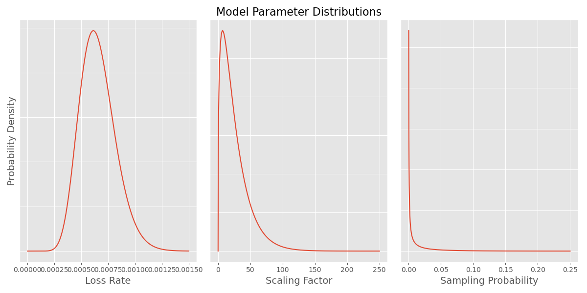
Figure 1: The posterior distributions for the loss rate $\lambda$, the scaling factor $a$, and the sampling probability $p$ for the Cyprus case study represent the combined information from the prior distributions and the survey data.

Parameter	Mean	Std. Dev.
Loss rate ($\lambda$)	0.00065	0.00017
Scaling factor ($a$)	25.78	22.03
Sampling probability ($p$)	0.01	0.03

Table 1: The summary statistics for the posterior distributions provide numerical estimates for the model parameters.

The mean and maximum a posteriori (MAP) estimates for the population at each time step are plotted in Figure 2. The shaded region represents the interquartile range of the posterior distributions, corresponding to 50% probability that the true population at each time step lies within the shaded region. The uncertainties in the population estimates are large, however the general trend of increasing population over time is clear, as is a probable period of more rapid population growth around 7000 BCE, with a period of possible decline or stagnation between 5000 BCE and 2000 BCE, followed by a period of more rapid growth potentially corresponding to the establishment of complex societies on the island.

Because of the size of the uncertainty, the effects of short-term demographic changes caused by events such as natural disasters, epidemics, or warfare, are difficult to detect without model refinement and the addition of more data. However, the general trends in the population over time are clear, and the case study illustrates the utility of uncertainty estimates in avoiding the misinterpretation of noise in the data as signal.

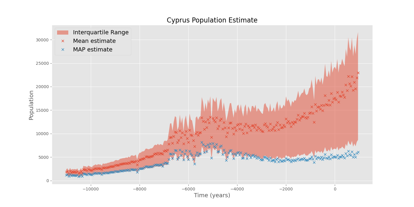
Figure 2: Large uncertainties in the population estimates are visible, however the general trend of increasing population over time is clear in both the mean and maximum a posteriori (MAP) estimates.

5 Discussion and Conclusion

The framework presented here provides a general method for estimating sizes and distributions of populations in the past. The framework is flexible and allows for extensions beyond the simple model demonstrated in the case study to capture more complex phenomena by increasing model expressivity, and to reduce uncertainties by incorporating additional data and prior information.

A clear approach to reducing uncertainties in the model and improving the sensitivity to demographic changes is to increase the quantity and quality of the data. This can be done by increasing the sizes of survey areas, such as through the use of extensive survey techniques reliant upon remote sensing, or by integrating more individual surveys. Additional intensive surveys can also increase the quantity of data and can be used to calibrate the sampling probabilities for the extensive surveys and to better estimate the distribution of settlement sizes in a region as a function of time. Another key element of data quality is ensuring the accuracy and precision of site chronology. Aspects of this include increasing the quantity of radiocarbon dates for sites and calibrating stratigraphy and artifact typologies to increase the quantity of available chronological data and better constrain and account for chronological uncertainty.

Because the loss rates, scaling factors, and scaling exponents will differ between proxies, these contributions to final estimate uncertainty can be reduced by increasing the variety of different proxies identified in a region. All else being equal, the contribution from each of these sources to the final estimate uncertainty will scale inversely with the square root of the number of proxies under consideration.

Estimates can also be improved and uncertainties can be reduced through better model construction. For example, better priors for model parameters can be determined either through reducing the uncertainties in individual model parameter distributions or through identifying functional forms for the distributions that better match prior knowledge. Increasing the depth of the hierarchical elements of the model can also allow for more precise control over confounding variables, although increasing model dimensionality also increases the quantity of data required for meaningful inference. Using non-parametric density estimation techniques such as MCMC also yields an advantage by increasing the expressivity of the posterior distributions, not limiting them to a particular family of distributions as is the case in variational approaches.

The sampling probabilities can be better constrained through increasing the fraction of the area under consideration that has been surveyed for the relevant proxy. Other calibration techniques can also be used to estimate sampling probabilities for specific surveys, such as through the comparison of different techniques in surveys with overlapping areas. Surveys and excavations from a variety of landscapes and environments can be used to attempt to control for biases in the geographic distribution and for variations in land-use, landscape productivity, and terrain.

Incorporating more specific prior knowledge about the behavior of populations through the development of parametric population models holds particular promise for more efficient and accurate inference. For example, the simple model discussed in Section 4 assumes no relationship between the population at time $t$ and the population at time $t+1$. Incorporating a parametric model without artificially limiting expressivity, as is the case in standard logarithmic or exponential regression, poses a challenging task.

In addition to enforcing a relationship between time $t$ and time $t+1$, a natural extension of the framework would be to incorporate a relationship between position $x$ and position $x+1$. This would allow for treatment of the locality assumption and for the capture of shifting population centers, for example due to local environmental variability. This could be done through the subdivision of the region under consideration into some grid or other tiling and the imposition of a distance metric. The model could then capture not only increases and decreases in population at one particular point or region, but movement of populations between regions, for example through the development of a discrete spatial diffusion model.

The case study presented in Section 4 demonstrates the utility of the framework to produce population estimates with a simple model and a single proxy, while ensuring that noise is not misinterpreted as signal—allowing for confidence in the validity of the results. The model extensions discussed above promise to capture more complex phenomena with more complex datasets, which would allow for better model construction and comparison, and could enable the testing of demographic, social, and technological theories with archaeological data.

References

- [1] Andrew Chamberlain “Demography in archaeology”, Cambridge manuals in archaeology Cambridge; New York: Cambridge University Press, 2006
- [2] E.T. Jaynes “Probability Theory: The Logic of Science” Cambridge University Press, 2003
- [3] Andrew Gelman et al. “Bayesian Data Analysis” CRC Press, 2020 URL: http://www.stat.columbia.edu/~gelman/book/
- [4] Katherine A. Crawford and Marc-Antoine Vella “Cyprus Dataset: Settlements from 11000 BCE to 1878 CE” In Journal of Open Archaeology Data 10, 2022, pp. 7 DOI: 10.5334/joad.96
- [5] Eli Bingham et al. “Pyro: Deep Universal Probabilistic Programming” In Journal of Machine Learning Research, 2018
- [6] Frederick W. Barry “Census of Cyprus, 1881” Proquest LLC, 2006
- [7] R.I.M. Dunbar “Neocortex size as a constraint on group size in primates” In Journal of Human Evolution 22.6, 1992, pp. 469–493 DOI: 10.1016/0047-2484(92)90081-J
- [8] E.. Crema “Statistical Inference of Prehistoric Demography from Frequency Distributions of Radiocarbon Dates: A Review and a Guide for the Perplexed” In Journal of Archaeological Method and Theory, 2022 URL: https://doi.org/10.1007/s10816-022-09559-5
- [9] Enrico R Crema and Andrew Bevan “Inference From Large Sets of Radiocarbon Dates: Software and Methods” In Radiocarbon 63.1, 2021, pp. 23–39 DOI: 10.1017/RDC.2020.95
- [10] Darcy Bird et al. “p3k14c, a synthetic global database of archaeological radiocarbon dates” In Scientific Data 9.1, 2022, pp. 27 DOI: 10.1038/s41597-022-01118-7
- [11] Val Attenbrow and Peter Hiscock “Dates and demography: are radiometric dates a robust proxy for long-term prehistoric demographic change?” In Archaeology in Oceania 50, 2015, pp. 30–36 DOI: 10.1002/arco.5052
- [12] Lorena Becerra-Valdivia, Rodrigo Leal-Cervantes, Rachel Wood and Thomas Higham “Challenges in sample processing within radiocarbon dating and their impact in 14C-dates-as-data studies” In Journal of Archaeological Science 113, 2020, pp. 105043 DOI: 10.1016/j.jas.2019.105043
- [13] W. Carleton and Huw S Groucutt “Sum things are not what they seem: Problems with point-wise interpretations and quantitative analyses of proxies based on aggregated radiocarbon dates” In The Holocene 31.4, 2021, pp. 630–643 DOI: 10.1177/0959683620981700
- [14] William A. Brown “Through a filter, darkly: population size estimation, systematic error, and random error in radiocarbon-supported demographic temporal frequency analysis” In Journal of Archaeological Science 53, 2015, pp. 133–147 DOI: 10.1016/j.jas.2014.10.013
- [15] Todd A. Surovell et al. “Correcting temporal frequency distributions for taphonomic bias” In Journal of Archaeological Science 36.8, 2009, pp. 1715–1724 DOI: 10.1016/j.jas.2009.03.029
- [16] Robert J. DiNapoli et al. “Approximate Bayesian Computation of radiocarbon and paleoenvironmental record shows population resilience on Rapa Nui (Easter Island)” In Nature Communications 12.1, 2021, pp. 3939 DOI: 10.1038/s41467-021-24252-z
- [17] Michael Holton Price et al. “End-to-end Bayesian analysis for summarizing sets of radiocarbon dates” In Journal of Archaeological Science 135, 2021, pp. 105473 DOI: 10.1016/j.jas.2021.105473
- [18] John W. Rick “Dates as Data: An Examination of the Peruvian Preceramic Radiocarbon Record” In American Antiquity 52.1, 1987, pp. 55 DOI: 10.2307/281060
- [19] Jennifer C. French et al. “A manifesto for palaeodemography in the twenty-first century” In Philosophical Transactions of the Royal Society B: Biological Sciences 376.1816 The Royal Society, 2020 URL: http://dx.doi.org/10.1098/rstb.2019.0707