Experimental characterization of traction-separation laws for interlaminar fracture in geometrically-scaled composites using progressive digital image correlation and through-thickness deformation analysis

Abstract

This work is focused on the experimental characterization of traction-separation laws for cohesive modeling of mode-II interlaminar fracture in composites. For the experimental investigation, damage progression in end-notched flexure specimens under three-point bending was captured using microscopic and macroscopic Digital Image Correlation (DIC) techniques. The specimens were geometrically scaled with three scaling levels for a size effect study. The fracture energy of the material was analyzed based on both linear elastic fracture mechanics and Bažant’s type-II size effect law for comparison. For damage modeling, traction-separation laws were built from the experimental data, and the fracture process zones of the specimens were modeled using cohesive interactions. Difficulties in characterizing traction-separation laws merely relying on load-displacement curves (i.e., global behaviors) were demonstrated and discussed through extensive simulations. To address this issue, through-thickness deformation analysis and progressive DIC methods were proposed and implemented in this work. The observations and proposed methods herein will contribute to characterizing a single traction-separation law for a given composite material by capturing global and local fracture behaviors on any geometric scale.

1 Introduction

1.1 Quasibrittle fracture process and size effect in composites

The anisotropy and heterogeneity of composites lead to complex damage progression compared to fracture and fatigue in isotropic and homogeneous materials [1]. The fracture process in composites shows quasibrittle characteristics, which are compared with well-known brittle and ductile cases in Fig. 1 for mode-I fracture. The degree of brittleness and ductility of materials is dictated by the size of Fracture Process Zones (FPZs) in front of crack tips [2]. The size of FPZs in brittle materials (see Fig. 1a) is so small that Linear Elastic Fracture Mechanics (LEFM) are applicable, while a large nonlinear plastic (or yielding) zone is observed in the form of a horizontal yield plateau (see Fig. 1b) in the FPZs of ductile or elastoplastic materials (mainly metals). The quasibrittle fracture process (see Fig. 1c) does not demonstrate notable plastic behaviors due to its negligible hardening area; however, quasibrittle materials can deliver large cracking opening displacements with the formation of extensive softening areas compared to brittle materials.

For experimental characterization of the interlaminar fracture energy (or toughness) of quasibrittle materials, Williams [3] and Davidson et al. [4, 5] proposed compliance calibration methods based on LEFM for mode I and II, respectively. These methods have been adopted in the ASTM standards [6, 7]. Salviato et al. [8], however, experimentally characterized mode-I and mode-II quasibrittle fracture processes in geometrically scaled composites and showed that these LEFM-based methods estimate multiple fracture energies for a single material (i.e., higher fracture energies with higher scaling factors). This analysis result contradicts the fact that fracture energies are unique material properties. To address this issue, they applied Bažant’s type-II size effect law [9] to the experimental load-displacement data in conjunction with numerical J-integral analysis [10] and obtained the fracture energy of the specimen material as a single value.

1.2 Damage modeling for composites

The Virtual Crack Closure Technique (VCCT) and cohesive zone models (CZMs) have widely been used for damage modeling for composites. Rybicki and Kanninen [11] proposed VCCT based on the LEFM principles to evaluate stress intensity factors in homogeneous isotropic materials. A thorough review of the technique can be found in Ref. [12]. The LEFM-based technique, however, has several drawbacks for composite damage modeling. To be specific, VCCT requires a precrack and a very fine mesh near the crack tip; additionally, complex moving mesh techniques are needed to advance the crack front [13]. On the other hand, CZMs can be applied to composites having no existing crack and a mesh around CZMs does not need to be modified to simulate damage progression. The early concepts of CZMs were proposed by Barenblatt [14], Dugdale [15], and Hillerborg [16]. Each composite material would have a single traction-separation law as its material property and thus the fracture mechanisms of CZMs for the material should follow the law. Detailed discussions on the characteristics of CZMs can be found in Ref. [17], while Refs. [13, 18, 19] presented thorough reviews of CZMs.

de Moura et al. [20, 21, 22] experimentally characterized CZMs for mode-I and mode-II fracture in adhesive-bonded joints. They adopted a Digital Image Correlation (DIC) technique to measure the separation of the crack tip from two DIC data points above and below the crack tip. Traction values were estimated based on Timoshenko beam theory. Their simulation results showed a good agreement with the experimental data. Compared to composites, adhesive-bonded joints show more stable crack growth (dependent on the sizes of the joints) with larger separation values, which are beneficial to the experimental characterization of their CZM parameters. Composites, on the other hand, show unstable crack propagation in mode II with a sudden drop (or a snapdown) of applied load induced by snapback instability [23, 24] under small separation between layers. These characteristics make CZM characterization for composites more challenging. Khaled et al. [25] applied a similar approach to T800S/F3900 carbon/epoxy unidirectional composites for mode-I and mode-II CZM characterization. Precracking was performed to propagate $5$ mm-long precracks from Teflon inserts in the specimens. They measured separations by manually selecting two DIC data points above and below the potential crack tip locations while estimating traction values using a closed-form solution for the J-integral [26] based on a compliance calibration method. The CZMs showed good performance overall; however, with underestimated maximum loads from the simulations, they reported difficulties in exactly locating the crack tips on DIC images and accurately capturing the separations with their DIC resolution. It should be noted that all these studies used single specimen sizes.

1.3 Challenge problem

Composites have been extensively adopted in modern aircraft designs. Half of the airframe and primary structures of the Boeing 787 (a subsonic commercial airliner), for example, are made up of Carbon Fiber-Reinforced Plastic (CFRP) and other composites [27]. A supersonic fighter, the Lockheed F-35 also has CFRP composite fuselage and wing structures [28]. Wiebe and Kim [29] showed that high-speed aircraft could experience amplified stress fields and possibly mode-II fatigue failure induced by aerothermodynamic couplings (see Fig. 2). To address this issue, this paper focuses on a specific challenge problem: mode-II interlaminar fracture in geometrically scaled End-Notched Flexure (ENF) composites in three-point bending tests. The focus on end-notched laminated composites was motivated by the fact that while still highly complex, the knowledge of likely crack planes (i.e., FPZs) induced by delamination is very helpful in developing damage models. Additionally, it is hoped that this work can form part of an experimental framework for characterizing traction-separation laws for quasibrittle materials in different geometries and loading environments. The challenge problem herein, for example, focuses on mode-II interlaminar fracture and laminated polymer matrix composite structures, which are of growing relevance in the aerospace industry. However, the framework obtained from this work can be directly applied to other fracture modes or mechanisms and other composite materials such as ceramic matrix composites for hypersonic vehicles [30]. Lastly, the current challenge problem will contribute to building an important bridge between the degradation of the mode-II traction-separation law parameters under fatigue loading and the fatigue failure of high-speed aircraft under aerothermodynamic loads.

1.4 Objectives

The objective of the work herein is to develop, propose, and implement part of an experimental framework for characterizing high-fidelity traction-separation laws for robust cohesive zone modeling of interlaminar fracture in quasibrittle composite materials based on full-field measurement of this process. The proposed framework aims to find traction-separation law parameters which can incorporate a size effect in quasibrittle fracture and thus consistently capture damage progression in geometrically scaled composites on both global and local scales. Characterizing the parameters directly from experimental data without employing complex analytical equations is of primary interest. It needs to be noted that the work presented in this paper is not focused on obtaining an exact traction-separation law for the challenge problem, which will be presented in a separate paper. This paper instead focuses on exposing issues related to the experimental characterization of a quasibrittle fracture process in composites from a single-size data set, discussing difficulties in calibrating and validating traction-separation laws on a global level (i.e., using load-displacement curves), and describing and implementing proposed methods to address these issues. This paper is organized in the following sequence: the specimen information and experimental setup are described in Section 2; the local and global analysis of the experimental data with a size effect study is presented in Section 3; the modeling details and simulation results are shown with discussions on difficulties in finding traction-separation laws in Section 4; the progressive DIC analysis of in-plane displacement through the thickness is proposed and implemented in Section 5; finally, the conclusions of this paper are presented in Section 6.

2 Experimental work

2.1 Specimen details

Composite specimens were laid up using the Toray T700G/2510 carbon fiber/epoxy prepreg system and were cured in an autoclave. The prepreg system has unidirectional T700G carbon fibers with the lamina/laminate mechanical properties given in Table 1. The specimens had an initial delamination in the midplane at the one end induced by embedded inserts. Others have studied another method of inducing precracks in specimens by applying mechanical or fatigue loads [31, 32, 33]. These methods, however, could induce unintended initial damage to FPZs in front of designed crack-tip locations in the form of microcracks. In this work, keeping the FPZs intact prior to fracture tests was crucial to the experimental characterization of traction-separation law parameters. Thus, this work employed the method of embedding non-adhesive inserts before curing to induce the precracks in the specimens. A DuPont Teflon^® FEP film ($12.7$ µm-thick) was adopted as an insert to meet the ASTM D7905/D7905M-19e1 specification of non-adhesive film insert type and thickness [7].

For a size effect study, the ENF specimens were geometrically scaled in three levels as shown in Fig. 3. The direction of the unidirectional fibers (i.e., the principal material axis $1$ [34]) was aligned with the $x$-axis prior to three-point bending tests, while the principal material axes $2$ and $3$ were parallel to the geometric axes $y$ and $z$, respectively. The dimensions of the Size-3 specimens were determined based on the ASTM D7905/D7905M-19e1 specification [7] and were used as a baseline for scaling. Given the beam characteristics of these specimens, 2D scaling of the geometric dimensions on the $x$–$z$ plane was made. To be specific, the gauge length $L$, thickness $h$, and initial crack length $a_{0}$ of the Size-3 set were scaled, while the width $b$ was kept constant. The target scaling factors were $1/2$ and $1/4$ for the Size-2 and the Size-1 set, respectively. Additionally, symmetric layups were required for all sizes to embed DuPont Teflon^® FEP films in the midplanes as inserts. To meet these requirements, the ASTM dimensions had to be slightly scaled up for the Size-3 specimens and 8, 16, and 32 plies of Toray T700G/2510 prepreg were laid up for Sizes 1, 2, and 3, respectively. The geometric dimensions of the scaled specimens are shown in Table 2. Four specimens were manufactured per each size and their actual dimensions $L$, $a_{0}$, $h$, and $b$ are tabulated in Table 3.

2.2 Experimental setup

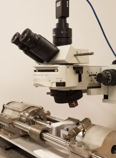
(a)

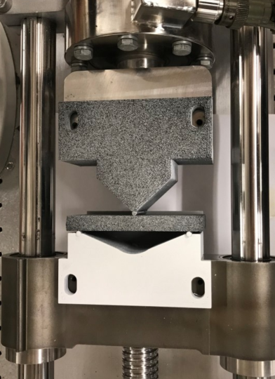
(b)

Figure 4: Experimental setup for the 2D microscopic DIC tests. (a) A psylotech µTS testing system along with an Olympus BXFM microscope. (b) A speckled ENF specimen in three-point bending fixtures.

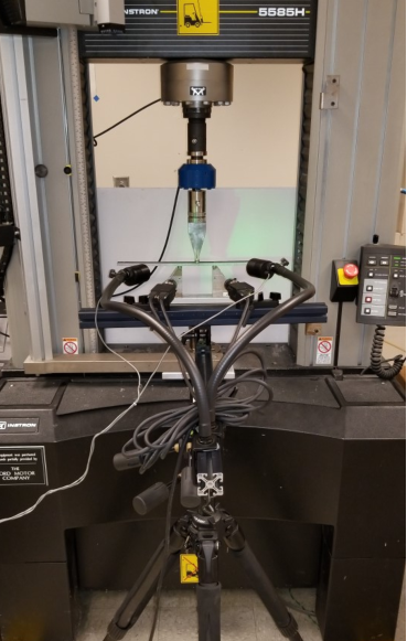
(a)

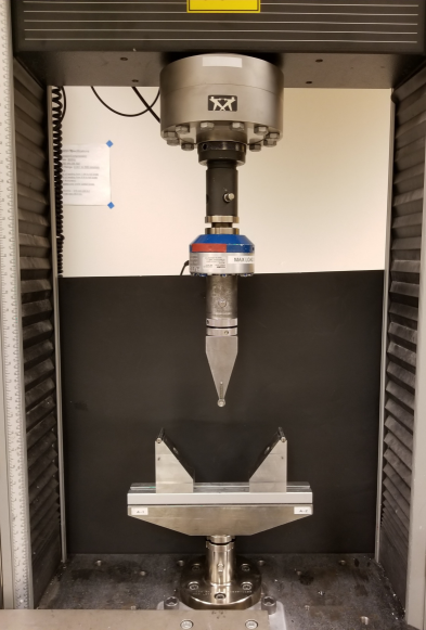
(b)

Figure 5: Experimental setup for the 3D macroscopic DIC tests. (a) An Instron 5585H testing system along with a Correlated Solutions VIC-3D DIC system. (b) Three-point bending fixtures.

For the experimental characterization of mode-II interlaminar fracture in these ENF specimens, quasi-static, monotonic three-point bending tests were conducted using a displacement control as shown in Figs. 4 and 5. Two different types of DIC systems were employed for the tests: a 3D macroscopic (or specimen-scale) and a 2D microscopic DIC system. For both cases, digital images were continuously captured at a constant interval from the beginning to the end of the tests to acquire full-field measurement data through DIC analysis. The microscopic-scale tests (see Fig. 4) were intended to capture detailed information on damage progression in the vicinity of the initial crack tips. Therefore, a small part of the specimen surface on the $x$–$z$ plane including the initial crack tip was captured in the digital images through the microscope. For these tests, a psylotech µTS testing system, an Olympus BXFM microscope, and a Correlated Solutions VIC-2D 2009 package [35] were used. The Size-1 and Size-2 specimens were tested using the microscopic DIC system; however, the Size-3 specimens could not fit into the system due to their large gauge lengths. The 3D macroscopic DIC system (see Fig. 5) was instead used for the Size-3 tests capturing structural response on the entire $x$–$z$ surface of the Size-3 specimens. An Instron 5585H testing system and a Correlated Solutions VIC-3D 7 system [36] were employed for the Size-3 specimen tests.

3 Experimental results

3.1 Experimental characterization of global behaviors

3.1.1 Load-displacement analysis

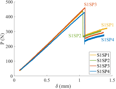
(a)

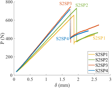
(b)

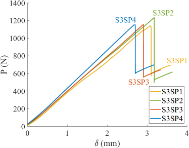
(c)

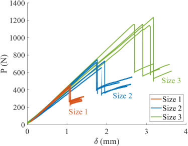
(d)

Figure 6: Experimental results of the ENF tests. The loads $P$ were applied through the cylindrical loading rollers (see Fig. 3) along the negative $z$–axis and the displacement values $\delta$ were also recorded at the loading points in the same direction. (a) Size-1 data. (b) Size-2 data. (c) Size-3 data. (d) Collection of all the test data.

The test results are illustrated in the form of load-displacement curves in Fig. 6 and their maximum (or critical) loads $P_{\text{max}}$ are tabulated in Table 5. The load-displacement data were intended to analyze the fracture energy of the specimen material and validate the global fracture behaviors simulated by numerical models. It needs to be noted that the horizontal testing configuration of the psylotech µTS testing system (see Fig. 4) required small preloads (around $40$ N) to keep the specimens in the fixtures prior to the tests and thus the load-displacement curves of the Size-1 and Size-2 specimens (see Figs. 6a and 6b) begin at the preloads. In Fig. 6d, the experimental data are plotted together to demonstrate the impact of geometric scaling on global fracture behaviors. The larger scaling factors led to higher $P_{\text{max}}$ than the smaller ones (i.e., the Size-3 set showed higher maximum loads than the Size-1 and Size-2 sets), while $P_{\text{max}}$ did not proportionally increase with an increase in the scaling factor. This size effect phenomenon will be explored in Section 3.1.2.

Using the load-displacement data, the LEFM fracture energies $G_{\text{f,LEFM}}^{\text{(II)}}$ of the specimens were estimated based on the compliance calibration methods described in the ASTM D7905/D7905M-19e1 testing manual. The superscript in $G_{\text{f,LEFM}}^{\text{(II)}}$ indicates the fracture mode of the property and will consistently be used for other fracture properties in this paper. For compliance calibration, the initial crack length $a_{0}$ was slightly decreased and increased to $a_{1}$ and $a_{2}$, respectively. The compliance crack lengths are tabulated for the three size sets in Table 2.

For completeness, some of the key equations in the manual are described here. Compliance calibration coefficients, labeled $A$ and $m$, are experimentally determined using a linear regression analysis of the compliance test data as shown below

$$\{C\}=A+m\{a^{3}\},$$ (1)

where $a_{i}$ and $C_{i}$ ($i=0,1,2$) are the crack lengths and corresponding compliance measurements, respectively. Using the coefficients, the fracture energy $G_{\text{f,LEFM}}^{\text{(II)}}$ of the material is calculated by

$$G_{\text{f,LEFM}}^{\text{(II)}}=\frac{3mP_{\text{max}}^{2}a_{0}^{2}}{2b},$$ (2)

where $P_{\text{max}}$ is the maximum load observed from the fracture tests with the initial crack length $a_{0}$. Additionally, the effective flexural moduli $\bar{E}_{\text{1f}}$ is given by

$$\bar{E}_{\text{1f}}=\frac{L^{3}}{4Abh^{3}},$$ (3)

where $L$, $b$, and $h$ are the specimen dimensions shown in Fig. 3.

The compliance measurements and calibration coefficients of the specimens are tabulated in Table 4, while $P_{\text{max}}$, $G_{\text{f,LEFM}}^{\text{(II)}}$, and $\bar{E}_{\text{1f}}$ are shown in Table 5. The manual specifies that the maximum load for the compliance calibration should lead to $\%G_{i}$ satisfying

$$15\leq\%G_{i}\leq 35,~{}~{}~{}i=1,2,$$ (4)

where

$$\%G_{i}=\Big{[}\frac{100(P_{i}a_{i})^{2}}{(P_{\text{max}}a_{0})^{2}}\Big{]},$$ (5)

and $P_{i}$ represents the maximum load applied for the crack length $a_{i}$. The compliance calibration values of $\%G_{i}$ ($i=1,2$) are also tabulated in Table 5. In this work, it was attempted to set $P_{i}$ satisfying the minimum $\%G_{i}$ requirement (i.e., $\%G_{i}\simeq 15$) to keep the FPZs intact prior to fracture tests. Among the twenty-four data sets (see Table 5), only $\%G_{1}$ of the S1SP3 specimen and $\%G_{2}$ of the S3SP1 specimen ($14.55$ and $14.78~{}\%$, respectively) could not meet the requirement but were still very close to the threshold value. It also needs to be noted that $\bar{E}_{\text{1f}}$ of the specimens were broadly consistent and thus the inconsistency in the load-displacement curve slopes of the same-size specimens (see Fig. 6) could be caused by some variance in the actual dimensions of the specimens.

3.1.2 Size effect analysis

As Salviato et al. [8] pointed out, $G_{\text{f,LEFM}}^{\text{(II)}}$ increases with the specimen size increase (see Table 5) and thus the LEFM-based compliance calibration method failed to characterize the fracture energy of the specimen material as a unique material property. To address this issue, Bažant’s type-II size effect law [9] was applied to the experimental data for fracture energy analysis. Detailed descriptions of the application of the size effect law can be found in the work of Salviato et al. [8, 37]. For completeness, some parts of these works are briefly introduced in this section. The mode-II interlaminar fracture energy $G^{\text{(II)}}_{\text{f}}$ and effective FPZ size $c^{\text{(II)}}_{\text{f}}$ of the material can be experimentally obtained as follows [38, 39]:

$$G^{\text{(II)}}_{\text{f}}=\frac{g_{\text{(II)}}(\alpha_{0})}{E^{*}B},~{}c^{\text{(II)}}_{\text{f}}=\frac{C}{B}\frac{g_{\text{(II)}}(\alpha_{0})}{g^{\prime}_{\text{(II)}}(\alpha_{0})},$$ (6)

where $g_{\text{(II)}}$ is the dimensionless energy release rate, $\alpha=a/h$ is the normalized effective crack length, and $E^{*}$ is the equivalent elastic modulus ($E^{*}=E_{\text{1t}}$ here). The constants $B$ and $C$ in Eq. 6 can be obtained through a linear regression analysis as follows:

$$Y=BX+C,$$ (7)

where $Y=\sigma_{\text{Nc}}^{-2}$ and $X=h$. The nominal strength $\sigma_{\text{Nc}}$ can be given by

$$\sigma_{\text{Nc}}=\frac{P_{\text{max}}}{bh}.$$ (8)

Finally, the size effect plot can be obtained using the following equation:

$$\sigma_{\text{Nc}}=\frac{\sigma_{0}}{\sqrt{1+h/h_{0}}},$$ (9)

where the pseudo-plastic limit $\sigma_{0}$ and the transitional characteristic length $h_{0}$ are given by

$$\sigma_{0}=\sqrt{\frac{G^{\text{(II)}}_{\text{f}}E^{*}}{c^{\text{(II)}}_{\text{f}}g^{\prime}_{\text{(II)}}(\alpha_{0})}},~{}h_{0}=\frac{c^{\text{(II)}}_{\text{f}}g^{\prime}_{\text{(II)}}(\alpha_{0})}{g_{\text{(II)}}(\alpha_{0})}.$$ (10)

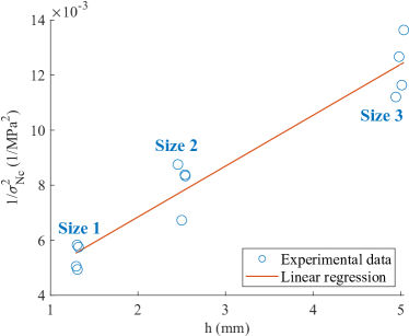
(a)

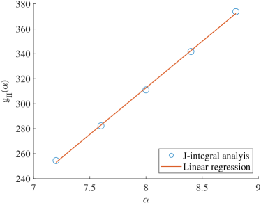
(b)

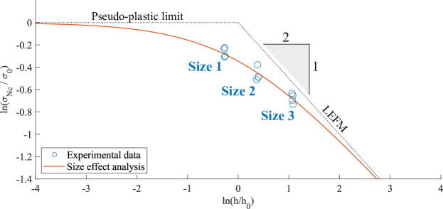
(c)

Figure 7: Size effect analysis of the experimental data. (a) Linear regression analysis to obtain the constant $A$ shown in Eq. 6. (b) J-integral simulation results. (c) Size effect plot.

The nominal strengths $\sigma_{\text{Nc}}$ of the specimens are tabulated in Table 5 and the size effect analysis result is presented in Fig. 7. The linear regression result in Fig. 7a showed $B=1.847\times 10^{-3}~{}\text{mm}^{3}/\text{N}^{2}$ and $C=3.155\times 10^{-3}~{}\text{mm}^{4}/\text{N}^{2}$. The dimensionless values $g_{\text{(II)}}$ and $g^{\prime}_{\text{(II)}}$ were obtained from the J-integral analysis of a nominal Size-2 specimen using the Abaqus/Standard solver [40]. The modeling details can be found in Refs. [8, 37]. The nominal dimensions of the Size-2 specimen (see Table 2) were used for modeling, while additional simulation data were obtained by changing the initial crack length $a_{0}$ by $\pm 1$ and $\pm 2$ mm. The modeling results are illustrated in Fig. 7b with $g_{\text{(II)}}(\alpha_{0})=311.1$ where $\alpha_{0}=8$. The dimensionless value $g^{\prime}_{\text{(II)}}(\alpha_{0})$ was obtained as $g^{\prime}_{\text{(II)}}(\alpha_{0})=74.56$ through linear regression of the modeling data. Substituting these values into Eq. 6, the fracture energy and effective FPZ size of the specimen material was obtained as $G^{\text{(II)}}_{\text{f}}=1.347$ N/mm and $c^{\text{(II)}}_{\text{f}}=7.126$ mm, respectively. Additionally, the pseudo-plastic limit $\sigma_{0}$ and the transitional characteristic length $h_{0}$ were obtained as $\sigma_{0}=17.80\text{ MPa}$ and $h_{0}=1.708\text{ mm}$ by Eq. 10. Finally, the size effect plot was drawn based on Eq. 9 as shown in Fig. 7c. The plot shows that the geometrically scaled specimens well captured both the pseudo-plastic limit and LEFM regime. To be specific, the Size-3 specimens were large enough to be in close proximity to the LEFM regime, while the thickness dimensions of the Size-1 set were scaled down enough to be smaller than the transitional characteristic length $h_{0}$.

3.2 Experimental characterization of local behaviors

3.2.1 Digital image correlation analysis

DIC analysis of the experimental data was performed to capture the local fracture process along the FPZs in front of the initial crack tips in the specimens. The DIC data were collected from the fracture tests of all the specimens. Given the large size of the DIC data, however, a single case was selected from each size set and was focused on in this paper. To be specific, the S1SP4, S2SP4, and S3SP3 data sets (see Table 3 for the specimen details) were chosen for more detailed analysis. These selections were made by evaluating discrepancies between the nominal and actual dimensions of the specimens and consistencies in their compliance calibration test results. As described in Section 2.2, the S1SP4 and S2SP4 specimens were tested using the 2D microscopic DIC system, while the 3D macroscopic DIC system was used for the S3SP3 specimen.

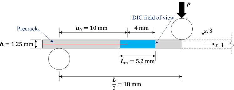
(a)

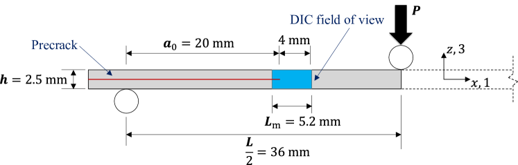
(b)

Figure 8: The field of view of the microscopic DIC system is schematically illustrated. The field length is represented by $\boldsymbol{L}_{\text{m}}$. The specimens are presented here in their undeformed configurations where the axes $1$ and $3$ are aligned with the axes $x$ and $z$, respectively. (a) A half of the nominal Size-1 specimen. (b) A half of the nominal Size-2 specimen.

The field of view of the microscopic DIC system is illustrated in Fig. 8. The view length $L_{\text{m}}$ includes $1.2$ mm of the precrack and $4$ mm of the predicted crack path (i.e., the potential FPZ). The principal material axes $1$ and $3$ were aligned with the geometric axes $x$ and $z$, respectively, prior to loading. The resolution of the digital images captured from the microscope was 2448$\times$2048 pixels. These images were processed for 2D DIC with a subset size [41] of 51$\times$51 pixels and a step size of 5$\times$5 pixels using the VIC-2D 2009 package.

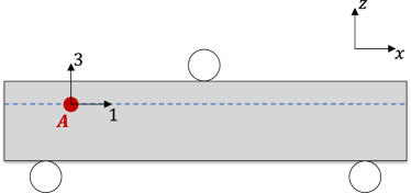
(a)

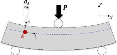
(b)

Figure 9: Schematic drawings of beam bending and axis rotation. The geometric coordinate system of the beam is shown by axes $x$ and $z$, while the principal material coordinate system at point $A$ is represented by axes $1$ and $3$. (a) The undeformed configuration of the beam prior to loading. (b) The deformed configuration of the beam under three-point bending. The material axes $1$ and $3$ rotated through angle $\theta_{A}$.

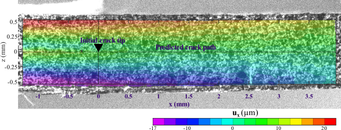
(a)

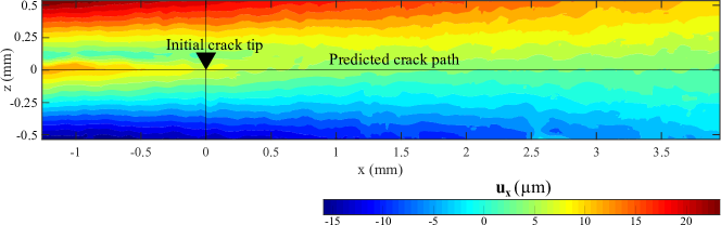
(b)

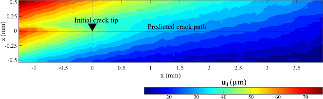
(c)

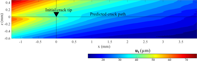
(d)

Figure 10: Post-processing steps for coordinate transformation and data smoothing of the raw DIC data of the S1SP4 specimen at $P_{\text{max}}$. The contours are presented in the undeformed configuration of the specimen where the axes $1$ and $3$ were aligned with the axes $x$ and $z$, respectively. (a) The contours of the raw DIC data of $u_{x}$ obtained using the VIC-2D 2009 package. The contours of $u_{x}$ were superimposed on the speckled specimen. (b) The contours of $u_{x}$ obtained by processing the raw DIC data using Matlab R2021a. (c) The contours of $u_{1}$ obtained by transforming the $u_{x}$ data from the $x$–$z$ coordinate system to the $1$–$2$ coordinate system. (d) The contours of $u_{1}$ obtained through data smoothing using Matlab R2021a.

The principal material axes rotated with specimen bending, while the geometric axes were fixed. This phenomenon is schematically illustrated in Fig. 9. The raw VIC-2D data were obtained along the geometric axes; for example, displacements were measured in the axes $x$ and $z$ and were named $u_{\text{x}}$ and $u_{\text{z}}$, respectively. For experimental characterization of interlaminar fracture along the fiber direction (i.e., the principal material axis $1$), a post-processing method was developed in this work to perform coordinate transformation and data smoothing of the VIC-2D data. The post-processing steps are illustrated in Fig. 10 with an example of obtaining the in-plane displacement $u_{1}$ in the $1$-axis of the S1SP4 specimen at the maximum load $P_{\text{max}}$. The contours in the figures were drawn in the undeformed configuration of the specimen where the axes $1$ and $3$ were aligned with the axes $x$ and $z$, respectively. In Fig. 10a, the contours of the raw data $u_{x}$ at $P_{\text{max}}$ are superimposed on the corresponding digital image of the speckled S1SP4 specimen. The raw data were initially interpolated using the griddata function of Matlab R2021a [42] (see Fig. 10b). The rotation angle of each data point was calculated based on the beam theories and the data were transformed from the $x$–$z$ coordinate system to the $1$–$3$ coordinate system as shown in Fig. 10c. Finally, the transformed data were smoothed using the polyfit function of Matlab R2021a (see Fig. 10d).

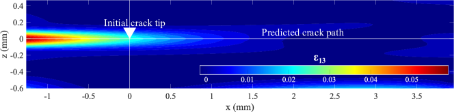
(a)

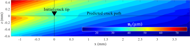
(b)

Figure 11: Microscopic DIC analysis of the S1SP4 data at $P_{\text{max}}$. The contours are presented in the undeformed configuration of the specimen where the axes $1$ and $3$ were aligned with the axes $x$ and $z$, respectively. (a) The contours of the out-of-plane shear strain $\varepsilon_{\text{13}}$ in the vicinity of the crack tip. (b) The contours of the in-plane displacement $u_{1}$ in the vicinity of the crack tip.

The post-processed microscopic DIC data of the S1SP4 and S2SP4 specimens at $P_{\text{max}}$ are presented in the forms of contour plots in Figs. 11 and 12, respectively. The contour plots of the S2SP4 specimen have the same length $L_{\text{m}}$ as the S1SP4 plots but cover larger surface areas due to the scaled-up thickness. It needs to be noted that the top and bottom boundary areas of the specimens were unevenly cut for the DIC analysis; as a result, the precracks and the predicted crack paths were not positioned in the middle of the contour drawings. As shown in Figs. 11a and 12a, large out-of-plane shear strains $\varepsilon_{13}$ were observed around the precrack and propagated along the predicted crack path. At the same time, the strongly zigzagging contours of in-plane displacement $u_{1}$ (see Figs. 11b and 12b) were formed in the precrack regions implying separation across the precrack. Weaker zigzags were observed from the $u_{1}$ contours near the initial crack tip along the predicted crack path, while nearly linear contours (i.e., no separation) were formed away from the initial crack tip.

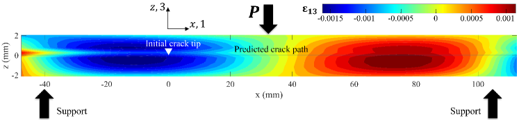
(a)

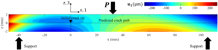
(b)

Figure 13: 3D DIC analysis of the S3SP3 data at $P_{\text{max}}$. For better visualization, the $z$–axis is exaggerated. The contours are presented in the undeformed configuration of the specimen where the axes $1$ and $3$ were aligned with the axes $x$ and $z$, respectively. (a) The contours of the out-of-plane shear strain $\varepsilon_{\text{13}}$ on the entire $x$–$z$ plane of the specimen. (b) The contours of the in-plane displacement $u_{1}$ on the entire $x$–$z$ plane of the specimen.

The 3D macroscopic DIC system covered the entire surface of the S3SP3 specimen on the $x$–$z$ plane. The resolution of the digital images captured from the two cameras was 2448$\times$2048 pixels. The images were processed for 3D DIC with a subset size of 35$\times$35 pixels and a step size of 7$\times$7 pixels using the VIC-3D 7 package. The macroscopic DIC data were also post-processed using Matlab R2021a for coordinate transformation and data smoothing. The post-processed data of $\varepsilon_{13}$ and $u_{1}$ at $P_{\text{max}}$ are presented in the forms of contour plots in Fig. 13. Similar to the microscopic data, relatively large $\varepsilon_{13}$ and the strongly zigzagging contours of $u_{1}$ were observed along the precrack and near the initial crack tip. The level of the details shown in the macroscopic DIC data, however, was significantly lower than the microscopic data as expected.

3.2.2 Through-thickness analysis of in-plane displacement

For a detailed analysis of local fracture behaviors, this work proposes a through-thickness analysis of in-plane displacement. In this method, the DIC data sets were further analyzed in the form of $u_{1}$ variation through the thickness (i.e., the $z$–axis). This analysis was intended to characterize the evolution of separation during the interlaminar fracture process.

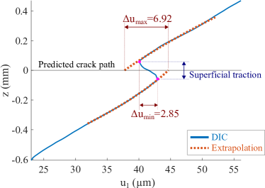
(a)

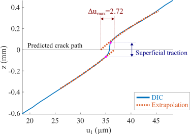
(b)

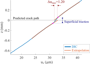
(c)

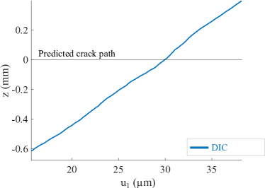
(d)

Figure 14: In-plane displacement $u_{1}$ variation through the thickness (i.e., the $z$–axis) of the S1SP4 specimen. The data were extracted from the contours of $u_{1}$ shown in Fig. 11b. (a) At $x=0$. (b) At $x=0.7$ mm. (c) At $x=1.5$ mm. (d) $x=2.0$ mm.

For the S1SP4 specimen at $P_{\text{max}}$, $u_{1}$–$z$ plots were captured at four different locations along the predicted crack path as shown in Fig. 14. To be specific, Fig. 14a shows $u_{1}$ variation through the thickness at the initial crack tip (i.e., $x=0$), while Fig. 14d was obtained $2.0$ mm away from the initial crack tip (i.e., $x=2.0$ mm). A strongly zigzagging curve was obtained at the initial crack tip (see Fig. 14a). It should be noted that paints were sprayed on the specimen surface (i.e., the $x$–$z$ plane) to form black and white speckles for DIC. The strong zigzag implies partial or complete separation between the layers; however, the paint coat on the surface was not separated yet and formed effective superficial traction. The superficial traction led to the continuous zigzagging curve instead of discontinuity in the curve across the predicted crack path (i.e., the FPZ) induced by separation. To address this issue, separation values were estimated in this work by extrapolating the plots except the superficial traction parts, which predicted the maximum separation values, $\Delta u_{\text{max}}$. The minimums $\Delta u_{\text{min}}$ were obtained using the $u_{1}$ values at the beginning and end of the superficial traction parts. The actual separation magnitudes would exist between $\Delta u_{\text{max}}$ and $\Delta u_{\text{min}}$ and could be closer to $\Delta u_{\text{max}}$ than $\Delta u_{\text{min}}$. This will be further discussed in the following section by comparing these plots with numerical simulation results. Weaker zigzagging curves (i.e., possibly smaller separation magnitudes) were observed from the plots acquired at the locations away from the initial crack tip as shown in Figs. 14b and 14c in which $\Delta u_{\text{min}}$ could not be obtained. Nearly linear plots were observed at $x\geq 2.0$ mm, implying that the size of the FPZ formed in the S1SP4 specimen at $P_{\text{max}}$ could be around $2.0$ mm.

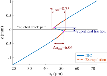
(a)

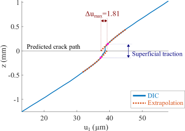
(b)

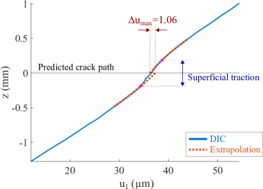
(c)

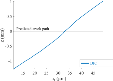
(d)

Figure 15: In-plane displacement $u_{1}$ variation through the thickness (i.e., the $z$–axis) of the S2SP4 specimen. The data were extracted from the contours of $u_{1}$ shown in Fig. 12b. (a) At $x=0$. (b) At $x=1.5$ mm. (c) At $x=2.0$ mm. (d) $x=3.0$ mm.

For analysis of separation in the S2SP4 specimen at $P_{\text{max}}$, the variation of $u_{1}$ through the thickness is presented in Fig. 15. The separation values $\Delta u_{\text{max}}$ and $\Delta u_{\text{min}}$ at the initial crack tip (see Fig. 15a) were larger than the corresponding values of the S1SP4 data Fig. 14a. At the same time, nearly linear plots were observed at $x\geq 3.0$ mm. This implies that the size of the FPZ formed at the S2SP4 specimen under $P_{\text{max}}$ could be around $3.0$ mm, which is larger than the FPZ size of the S1SP4 specimen.

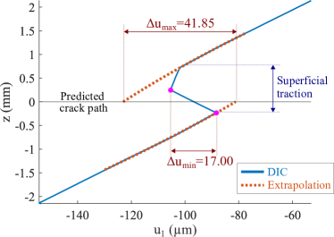
(a)

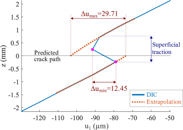
(b)

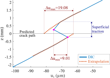
(c)

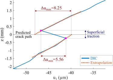
(d)

Figure 16: In-plane displacement $u_{1}$ variation through the thickness (i.e., the $z$–axis) of the S3SP3 specimen. The data were extracted from the contours of $u_{1}$ shown in Fig. 13b. (a) At $x=0$. (b) At $x=5.0$ mm. (c) At $x=10.0$ mm. (d) $x=18.0$ mm.

Lastly, the variation of $u_{1}$ through the thickness in the S3SP3 specimen at $P_{\text{max}}$ is further analyzed in Fig. 16. Significantly larger separation $\Delta u_{\text{max}}$ and $\Delta u_{\text{min}}$ were observed at the initial crack tip of the S3SP3 specimen (see Fig. 16a) compared to the S1SP4 and S2SP4 cases. High separation values were observed at $x\leq 18.0$ mm, while no linear variation was found due to the resolution of the 3D DIC data. Given a change in the sign of the $u_{1}$–$z$ plot slopes across $x=22.0$ mm (it can also be observed in the $u_{1}$ contour plots in Fig. 13b), the FPZ size of S3SP3 could be approximately $22.0$ mm. The separation values and FPZ sizes of these three specimens under $P_{\text{max}}$ are summarized in Table 6.

3.3 Discussions

The global-local analysis of the experimental data showed that $G_{\text{f,LEFM}}^{\text{(II)}}$ and $\Delta u_{\text{1}}$ at $P_{\text{max}}$ increased with an increase in the scaling factor. The $G_{\text{f,LEFM}}^{\text{(II)}}$ values of the Size-3 set (the most scaled-up set), however, were still smaller than the single fracture energy $G^{\text{(II)}}_{\text{f}}$ obtained using Bažant’s type-II size effect law. This phenomenon could imply that smaller energy was released at $P_{\text{max}}$ in the smaller (or more scaled-down) specimen due to partial CZM development at a lower $\Delta u_{\text{1}}$ level. The proposed experimental framework using a through-thickness analysis of in-plane displacement worked well for obtaining the separation values from the microscopic DIC data. However, finding the traction-separation law of the specimen material still remained challenging due to difficulties in the experimental characterization of the tractions. This issue will be further discussed in the following sections.

4 Formulation of traction-separation laws

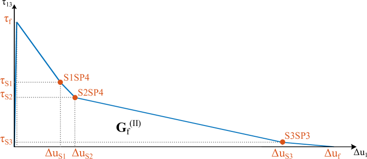
Figure 17: A schematic drawing of the traction-separation ($\tau_{\text{13}}$–$\Delta u_{\text{1}}$) law of the specimen material for mode-II interlaminar fracture. The complete separation, maximum traction, and fracture energy values are represented by $\Delta u_{\text{f}}$, $\tau_{\text{f}}$, and $G_{\text{f}}^{\text{(II)}}$, respectively. The separation levels observed in the S1SP4, S2SP4, and S3SP3 specimens at their maximum loads are shown as $\Delta u_{\text{S1}}$, $\Delta u_{\text{S2}}$, and $\Delta u_{\text{S3}}$, respectively, and the assumed corresponding tractions as $\tau_{\text{S1}}$, $\tau_{\text{S2}}$, and $\tau_{\text{S3}}$, respectively.

Based on the experimental observation, the traction-separation law of the specimen material for mode-II interlaminar fracture was schematically drawn as shown in Fig. 17. The area below the traction-separation curve corresponds to the fracture energy $G^{\text{(II)}}_{\text{f}}$ obtained from the size effect analysis. The piecewise softening curve was drawn based on the separation measurements in Table 6 and assumed corresponding traction values. Several CZM parameter sets were initially established based on the schematic traction-separation concept; however, their simulation results showed that partial CZM development is a complex mechanism and thus needs to be further investigated as a separate research topic. To address this issue, complete CZM development (or complete release of fracture energy) at $P_{\text{max}}$ was assumed for traction-separation law formulation in this paper. Therefore, the experimental separation measurements $\Delta u_{\text{max}}$ (see Table 6) were used as complete separation values. The experimental values $G^{\text{(II)}}_{\text{f,LEFM}}$ (see Table 5) were initially adopted as fracture energy parameters but were modified through global validation to find the energy levels released in the specimens at $P_{\text{max}}$. As a result, the CZM parameters for modeling the three representative specimens appeared to be very different; however, a single set of CZM parameters should exist for the specimen material as its material properties. This inconsistency was intended to expose many challenges in achieving a single traction-separation law for scaled specimens of a single quasibrittle material. Furthermore, the individually modified fracture energies were expected to provide important data on the actual energy release levels of the representative specimens at $P_{\text{max}}$ for further investigation on partial CZM development in future work. The validity of the traction-separation laws and related parameters were evaluated by comparing numerical modeling results with the experimental data in terms of local and global behaviors.

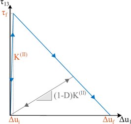
(a)

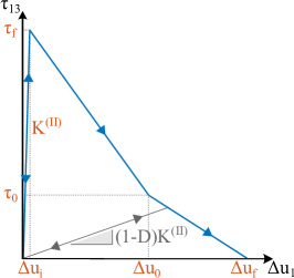
(b)

(c)

Figure 18: Different types of traction-separation ($\tau_{\text{13}}$–$\Delta u_{\text{1}}$) laws for mode-II interlaminar fracture. The initial interface stiffness, damage variable, damage initiation, final (or complete) separation, and maximum (or critical) traction are represented by $K^{\text{(II)}}$, $D$, $\Delta u_{\text{i}}$, $\Delta u_{\text{f}}$, and $\tau_{\text{f}}$, respectively. (a) CZM-L: Linear softening. (b) CZM-biL: Bilinear softening with a transition at $\Delta u_{0}$ and $\tau_{0}$. (c) CZM-pL: Initial plateau with subsequent linear softening at $\Delta u_{0}$–$\Delta u_{\text{f}}$.

For traction-separation ($\tau_{\text{13}}$–$\Delta u_{\text{1}}$) law formulation, many different types of laws were employed and evaluated in this work. The following will focus on three commonly used laws among them as shown in Fig. 18, while more complex laws will be described in a separate paper as highlighted in Section 1.4. The three traction-separation laws for mode-II interlaminar fracture have different softening laws: linear softening (see Fig. 18a), bilinear softening (see Fig. 18b), and initial-plateau with subsequent linear softening (see Fig. 18c). These laws are also called bilinear, trilinear, and trapezoidal forms, respectively, based on their whole curve shapes [43]. In this work, the laws led to three types of CZMs which were named CZM-L, CZM-biL, and CZM-pL for linear softening, bilinear softening, and plateau-linear softening laws, respectively. It should be noted that potential plastic deformations or dissipation at the initial crack tip [44] were not considered in these laws and will be investigated in future work.

All the laws have an initial elastic region with initial (or undamaged) interface stiffness $K^{\text{(II)}}$ up to the maximum (or critical) shear traction $\tau_{\text{f}}$. In the initial elastic region, the damage variable is zero (i.e., $D=0$). Detailed discussions on the damage variable can be found in Ref. [45]. Once $\tau_{\text{f}}$ is reached, damage progression is initiated at $\Delta u_{\text{i}}$ and the damage variable grows along the softening curves (i.e., $0<D\leq 1$). Under softening, the interface stiffness is reduced to $(1-D)K^{\text{(II)}}$. The areas below the traction-separation curves correspond to the fracture energy $G^{\text{(II)}}_{\text{f}}$ of the material for mode-II interlaminar fracture, which is completely released at the final (or complete) separation $\Delta u_{\text{f}}$ (i.e., $D=1$).

The initial interface stiffness was assumed to be $K^{\text{(II)}}_{\text{base}}=1\times 10^{6}$ MPa/mm based on the work of Turon et al. [46] and Zhao et al. [47] for T300/977-2 and T700/QY9511 carbon-fiber/epoxy composites, respectively. Having the value as a baseline, three different values $K^{\text{(II)}}=5\times 10^{4},~{}1\times 10^{5},~{}\text{and}~{}1\times 10^{7}$ MPa/mm were also adopted to investigate the impact of $K^{\text{(II)}}$ on modeling results. These values were chosen to cover the initial interface stiffness parameters reported in the literature which are summarized in Refs. [48, 49].

For modeling, Abaqus/CAE 2022 was employed and an identical modeling methodology was applied to the three models. Screenshots of the Abaqus S1SP4 model are presented in Fig. 19 to describe the modeling methodology. The upper and lower beam sections were modeled using 2D-planar (on the $x$–$z$ plane) deformable parts, while the loading and supporting rollers were generated using 2D-planar analytical rigid parts. These separate parts were assembled using contact interactions as shown in Fig. 19a. The cohesive zone additionally included cohesive and damage parameters based on the three traction-separation laws and was modeled along the midplane of the beam. The CZM parameters are tabulated in Table 7. Four-node bilinear plane strain quadrilateral, incompatible (CPE4I) elements [50, 51] were employed as shown in Fig. 19b. The three models had different sizes and numbers of elements based on the FPZ sizes of the corresponding specimens. The fracture process in these models was simulated using the Abaqus/Dynamic, Implicit solver with a quasi-static option.

4.1 S1SP4 model

The mesh on the S1SP4 model was composed of 235434 CPE4I elements and the size of the elements along the cohesive zone between the initial crack tip and loading point were 5$\times$5 µm. This element size was chosen to be small enough to capture the formation of FPZ during damage progression along the cohesive zone given that the FPZ size formed in the S1SP4 specimen at $P_{\text{max}}$ was observed to be approximately $2.0$ mm in the experiments.

4.1.1 Simulation results of the S1SP4 model based on $G^{\text{(II)}}_{\text{f,LEFM}}$

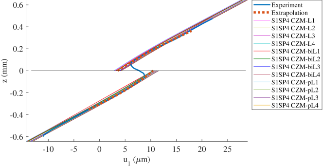
(c)

Figure 20: Traction-separation laws and simulation results of the S1SP4 model based on $G^{\text{(II)}}_{\text{f,LEFM}}$. (a) Traction-separation ($\tau_{\text{13}}$–$\Delta u_{\text{1}}$) laws adopted in the model. The parameters are tabulated in Table 7. (b) Load-displacement ($P$–$\delta$) curves simulated using the S1SP4 model with the $\tau_{\text{13}}$–$\Delta u_{\text{1}}$ laws shown in (a). The experimental curves in Fig. 6a were reproduced here for comparison. (c) In-plane displacement $u_{1}$ variation through the thickness at the initial crack tip under $P_{\text{max}}$. The experimental curve and its extrapolation in Fig. 14a were shifted here by $-33.1$ µm in the $u_{\text{1}}$ axis for comparison.

The simulation results of the S1SP4 model based on the $G^{\text{(II)}}_{\text{f,LEFM}}$ and $\Delta u_{\text{f}}$ values of the S1SP4 specimen are presented in Fig. 20. The CZM parameter sets in Table 7 led to twelve different traction-separation curves as shown in Fig. 20a. For global behavior validation, the load-displacement ($P$–$\delta$) curves of these twelve cases are presented altogether with the experimental data in Fig. 20b. The twelve CZMs led to almost identical $P$–$\delta$ curves and $P_{\text{max}}$; however, all the cases underestimated $P_{\text{max}}$ compared to the experimental one (around $-10$% error) as tabulated in Table 7. Additionally, local behavior validation was made by analyzing in-plane displacement $u_{\text{1}}$ at the initial crack tip under $P_{\text{max}}$ as shown in Fig. 20c. The twelve CZM cases showed similar $u_{\text{1}}$ through the thickness. It should be noted that the experimental $u_{\text{1}}$ curve and its extrapolations needed to be shifted by $-33.1$ µm in the $u_{\text{1}}$ axis for comparison with the simulation results. This phenomenon could have been caused by the different behaviors of the S1SP4 specimen and model at the supporting roller boundaries. The behavior of the specimen at the boundaries could not be captured in the field of view from the microscope; however, given the small scale of $u_{1}$ (i.e., a micron scale), the $u_{1}$ values would be extremely sensitive to the boundary motions. This issue will be further investigated in future work. The $u_{1}$ values of the experimental data and simulation results cannot be compared due to the shift; however, the slopes of all the simulation curves showed good agreement with the experimental one. Moreover, the extrapolated parts of the shifted experimental curve were in good agreement with the simulation results, which substantiates the presence of superficial traction along the FPZ induced by the surface paint. Therefore, the actual separation could be estimated by the extrapolated curves; that is, $\Delta u_{\text{max}}$ would be close to the actual separation values.

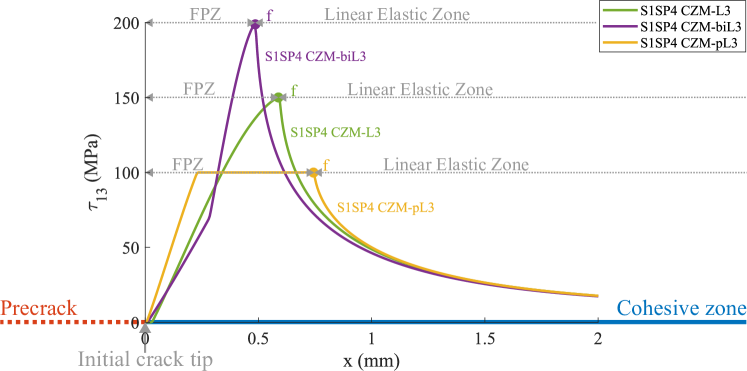
Figure 21: Distribution of traction $\tau_{\text{13}}$ between the upper and lower parts of the S1SP4 model at $P_{\text{max}}$.

Lastly, the distribution of traction $\tau_{13}$ between the upper and lower parts of the beam model at $P_{\text{max}}$ is illustrated in Fig. 21. These plots were intended to describe the FPZ development near the initial crack tip at $P_{\text{max}}$ and the impact of traction-separation types on the $\tau_{13}$ distribution along the CZM region. Among the twelve simulation cases, the three cases having the baseline initial interface stiffness were chosen here. The regions between the initial crack tip and $\tau_{\text{f}}$ were experiencing softening or complete separation and thus formed FPZs. For the CZM-L3 case, for example, the data points at $0\leq x\leq 0.56$ mm already reached $\tau_{\text{f}}$ prior to $P_{\text{max}}$ and were experiencing softening at $P_{\text{max}}$, while the adjacent region at $x>0.56$ mm did not reach $\tau_{\text{f}}$ and thus was staying in the linear elastic regime. Therefore, the FPZ size of the case at $P_{\text{max}}$ was $0.56$ mm. The FPZ sizes of all the cases at $P_{\text{max}}$ are tabulated in Table 7. For each $K^{\text{(II)}}$ value, the plateau-linear softening case formed the largest FPZ, while the smallest FPZ was shown in the bilinear case. All the cases showed significantly smaller FPZ sizes compared to the microscopic DIC analysis, $2.0$ mm. It was observed that the FPZ size increased with an increase in $K^{\text{(II)}}$ or a decrease in $\tau_{\text{f}}$.

4.1.2 Simulation results of the S1SP4 model based on modified $G^{\text{(II)}}_{\text{f,LEFM}}$

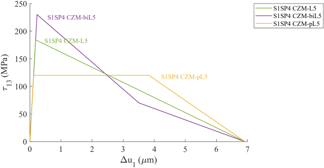
(a)

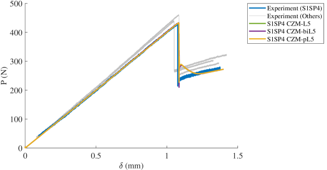
(b)

(c)

Figure 22: Traction-separation laws and simulation results of the S1SP4 model based on $G^{\text{(II)}}_{\text{f,mod}}$. (a) Traction-separation ($\tau_{\text{13}}$–$\Delta u_{\text{1}}$) laws adopted in the model. The parameters are tabulated in Table 8. (b) Load-displacement ($P$–$\delta$) curves simulated using the S1SP4 model with the $\tau_{\text{13}}$–$\Delta u_{\text{1}}$ laws shown in (a). The experimental curves in Fig. 6a were reproduced here for comparison. (c) In-plane displacement $u_{1}$ variation through the thickness at the initial crack tip under $P_{\text{max}}$. The shifted experimental curve in Fig. 20c was reproduced here for comparison.

It was observed that the S1SP4 model based on $G^{\text{(II)}}_{\text{f,LEFM}}$ underestimated $P_{\text{max}}$ for all the combinations of the three traction-separation laws and the four initial interface stiffness parameters. To address this issue, another traction-separation law set was generated as tabulated in Table 8. The fracture energy was increased to $G^{\text{(II)}}_{\text{f,mod}}=0.6375$ N/mm, while the complete separation values were maintained as $\Delta u_{\text{f}}=6.92$ µm. As a result, the maximum traction $\tau_{\text{f}}$ had to be increased for all the three cases. Only $K^{\text{(II)}}_{\text{base}}$ was adopted in these sets, which was justified by the fact that it had little effect as shown in Section 4.1.1. The simulation results are presented in Fig. 22. The three traction-separation curves shown in Fig. 22a were used for the simulations. As shown in Fig. 22b, all three CZM cases had excellent agreement with the experimental data. The $P_{\text{max}}$ values of the simulation cases showed $0.52$–$0.57\%$ errors compared to the experimental measurement (see Table 8). For local validation, the $u_{\text{1}}$ curves of the model at the initial crack tip under $P_{\text{max}}$ still showed good agreement with the shifted experimental curve as shown in Fig. 22c. It was observed that the increased fracture energy led to slightly higher deflections in the model compared to the experimental one. Finally, the FPZ size of the model at $P_{\text{max}}$ decreased compared to the corresponding cases shown in the previous section even though the fracture energy increased. This would imply that the FPZ size could be more affected by $\tau_{\text{f}}$ than $G^{\text{(II)}}_{\text{f}}$.

4.2 S2SP4 model

Given that the FPZ size of the S2SP4 specimen at $P_{\text{max}}$ was $3.0$ mm (see Table 6), the element size of the S2SP4 model along the cohesive zone between the initial crack tip and the loading point was chosen to be 10$\times$10 µm. As a result, the element mesh on the model was made of 312772 CPE4I elements.

4.2.1 Simulation results of the S2SP4 model based on $G^{\text{(II)}}_{\text{f,LEFM}}$

The CZM parameters used for the S2SP4 model based on the $G^{\text{(II)}}_{\text{f,LEFM}}$ and $\Delta u_{\text{f}}$ values of the S2SP4 specimen are tabulated in Table 9, while the simulation results are presented in Fig. 23. Similar to the S1SP4 cases, the dissimilar traction-separation curves in Fig. 23a led to the indistinguishable $P$–$\delta$ curves as shown in Fig. 23b; however, they all overestimated $P_{\text{max}}$ ($6.49$–$6.78$ % higher). For local validation, the experimental $u_{\text{1}}$ curve shown Fig. 15a was shifted by $-37.9$ µm in the $u_{\text{1}}$ axis for comparison with the simulation results in Fig. 23c. The $u_{\text{1}}$ curves of the S2SP4 model were almost identical but showed higher deflections than the experimental curve due to the larger $\delta$ values at $P_{\text{max}}$. Lastly, given the FPZ size of the S2SP4 specimen was $3.0$ mm (see Table 6), all the twelve CZM cases significantly underestimated the FPZ size as tabulated in Table 9.

4.2.2 Simulation results of the S2SP4 model based on modified $G^{\text{(II)}}_{\text{f,LEFM}}$

The $G^{\text{(II)}}_{\text{f,LEFM}}$ value of the S2SP4 specimen led to overestimated $P_{\text{max}}$. To address this issue, the fracture energy was reduced to $G^{\text{(II)}}_{\text{f,mod}}=0.75$ N/mm, maintaining $\Delta u_{\text{f}}=8.75$ µm. Therefore, the maximum traction $\tau_{\text{f}}$ values were reduced for the linear and plateau-linear softening cases (S2SP4 CZM-L5 and pL5, respectively), while only the transition traction $\tau_{\text{0}}$ value instead decreased for the bilinear softening case (S2SP4 CZM-biL5). Only $K^{\text{(II)}}_{\text{base}}$ was adopted in all three cases. The traction-separation parameters are tabulated in Table 10 and the simulation results are illustrated in Fig. 24. The three cases in Fig. 24a made an excellent agreement with the experimental $P$–$\delta$ curve as shown in Fig. 24b. The $P_{\text{max}}$ values of the S2SP4 model showed around $-0.1\%$ error compared to the experimental data. The $u_{\text{1}}$ curves of the model, however, still showed higher deflections than the experimental measurement as shown in Fig. 24c. Interestingly, the FPZ size of the model at $P_{\text{max}}$ increased for the linear and plateau-linear softening cases compared to the corresponding results shown in the previous section even though the fracture energy was reduced. This would substantiate the supposition that the FPZ size could be more sensitive to changes in $\tau_{\text{f}}$ rather than $G^{\text{(II)}}_{\text{f}}$. The increased FPZ sizes, however, were still significantly smaller than the experimental measurement. It should be noted that the CZM parameters, S1SP4 CZM-L5, biL5, and pL5, worked very well for the S1SP4 model (see Table 8); however, the S2SP4 model underestimated $P_{\text{max}}$ with these parameters as shown in Fig. 24b and Table 11.

4.3 S3SP3 model

The element size of the S3SP3 model along the cohesive zone between the initial crack tip and loading point was chosen to be $20$ µm $\times 20$ µm given the large FPZ size of the S3SP3 specimen, $22.0$ mm. The total number of CPE4I elements in the model was 310525.

4.3.1 Simulation results of the S3SP3 model based on $G^{\text{(II)}}_{\text{f,LEFM}}$

The CZM parameters for the S3SP3 model in Table 12 were initially obtained based on the $G^{\text{(II)}}_{\text{f,LEFM}}$ and $\Delta u_{\text{f}}$ values of the S3SP3 specimen. The simulation results are illustrated in Fig. 25. The twelve traction-separation curves were generated as shown in Fig. 25a. In contrast to the previous two models, the $K^{\text{(II)}}$ values did not make an apparent difference in the curve shapes due to the large $\Delta u_{\text{f}}$ value. The softening types, on the other hand, made a small difference in the $P$–$\delta$ curves as shown in Fig. 25b. The $P$–$\delta$ curves of the model showed marginal softening between $0.4P_{\text{max}}$ and $P_{\text{max}}$. The plateau-linear softening type showed the largest reduction in the stiffness, while the bilinear type experienced the smallest. All the twelve cases underestimated $P_{\text{max}}$ by $9.80$ – $10.02\%$ (see Table 12). The $u_{\text{1}}$ curves of the S3SP3 model showed lower deflections than the shifted experimental curve as shown in Fig. 25c due to the smaller $\delta$ values at $P_{\text{max}}$. Lastly, the FPZ sizes of the model at $P_{\text{max}}$ ($4.72$ – $9.50$ mm) were significantly smaller than the experimental measurement ($22.0$ mm) as shown in Table 12.

4.3.2 Simulation results of the S3SP3 model based on modified $G^{\text{(II)}}_{\text{f,LEFM}}$

For better model validation, the fracture energy was increased to $G^{\text{(II)}}_{\text{f,mod}}=1.20$ N/mm. The modified CZM values are tabulated in Table 13 and the simulation results are presented in Fig. 26. As shown in Fig. 26a, the $\Delta u_{\text{f}}$ of the S3SP3 specimen was still adopted in the traction-separation laws, while only $K^{\text{(II)}}_{\text{base}}$ was selected. As a result, the maximum traction $\tau_{\text{f}}$ values were increased for the linear and plateau-linear softening cases (S3SP3 CZM-L5 and pL5, respectively), while only the transition separation value $\Delta u_{\text{0}}$ instead increased for the bilinear softening case (S3SP3 CZM-biL5). The simulation results of the model showed good agreement with the experimental $P$–$\delta$ and $\tau_{\text{13}}$–$\Delta u_{\text{f}}$ curves as shown in Fig. 26b and Fig. 26c, respectively. For global behavior validation, the model showed $-0.91$ to $-1.71\%$ errors with respect to $P_{\text{max}}$; however, the marginal softening of the stiffness was still observed between $0.4P_{\text{max}}$ and $P_{\text{max}}$. The model also showed good agreement with the local behavior of the S3SP3 specimen as shown in the $\tau_{\text{13}}$–$\Delta u_{\text{f}}$ curves. It needs to be noted that the bilinear softening case showed a separation value smaller than $\Delta u_{\text{f}}$ at $P_{\text{max}}$. This would imply that the model experienced partial CZM development at $P_{\text{max}}$ under the bilinear softening law. Additionally, the FPZ size of the model was reduced for all three cases. The reduced sizes in the linear and plateau-linear softening cases could be attributed to the deceased $\tau_{\text{f}}$, while the partial CZM development could lead to the decreased FPZ size in the bilinear softening case.

The CZM parameters shown in Tables 8 and 10 worked very well for the S1SP4 and S2SP4 models, receptively. These parameters were also adopted in the S3SP3 model and the simulation results are shown in Fig. 26b and Tables 14 and 15. It was observed that the model significantly underestimated $P_{\text{max}}$ with these CZM parameters. The CZM parameters obtained from the S1SP4 model led to larger errors (or lower $P_{\text{max}}$) due to smaller $G^{\text{(II)}}_{\text{f}}$ than the parameters of the S2SP4 model.

4.4 Discussions

The experimental fracture energies $G^{\text{(II)}}_{\text{f,LEFM}}$ characterized for each specimen using the compliance calibration method led to the underestimated $P_{\text{max}}$ values in the S1SP4 and S3SP3 models and the overestimated ones in the S2SP4 model. The fracture energies and CZM parameters of the models were modified to match their simulation results with the corresponding experimental load-displacement curves. Each modified CZM parameter set worked very well for a specific model but did not for the other models; that is, the CZM parameters were highly sensitive to scaled sizes. This contradicts the fact that traction-separation laws are material properties and thus a single law exists for a quasibrittle material. For all the CZM parameters, the FPZ sizes of the models at $P_{\text{max}}$ were significantly smaller than the experimental measurements. It needs to be noted that all the modified fracture energies $G^{\text{(II)}}_{\text{f,mod}}$ were smaller than the fracture energy $G^{\text{(II)}}_{\text{f}}$ obtained from the Bažant’s type-II size effect analysis in Section 3.1.2. Furthermore, the insensitivity of the global behaviors (i.e., the load-displacement curves) to the initial interlaminar stiffness and traction-separation types was observed from the simulation results of the three models. That phenomenon made it extremely challenging to characterize the shape of the traction-separation laws by merely relying on load-displacement curve validation.

5 Progressive DIC analysis of in-plane displacement through the thickness

This work proposed a through-thickness analysis of in-plane displacement for local fracture analysis and characterized separation values $\Delta u_{\text{1}}$ as described in Section 3.2.2. The traction-separation laws of the specimen material were formulated based on the experimental measurement of $\Delta u_{\text{f}}$ assuming complete CZM development at the initial crack tip under $P_{\text{max}}$. The limitation of the model validation based on load-displacement ($P$–$\delta$) curves, however, was exposed from the extensive simulations as shown in Section 4. To address this issue, this work proposes a $P$–$\Delta u_{\text{1}}$ curve as an additional model validation tool. Characterizing $P$–$\Delta u_{\text{1}}$ curves is proposed here to synchronize global and local behaviors during a fracture process.

5.1 History of separation evolution in the form of $P$–$\Delta u_{\text{1}}$ curves

In the proposed method, the history of separation evolution at the initial crack tip of a specimen is characterized in a load-separation ($P$–$\Delta u_{1}$) space as shown in Fig. 27. The through-thickness analysis of $u_{1}$ was performed only at $P_{\text{max}}$ (i.e., at a single DIC frame) to characterize $\Delta u_{\text{f}}$ as presented in Section 3.2.2. For the experimental characterization of separation evolution, the through-thickness analysis was extended to all DIC frames (or data sets) between the initial and maximum load levels. The $P$–$\Delta u_{1}$ curves of the S1SP4 specimen (see Fig. 27a), for example, were characterized using 751 DIC data sets. For validation, separation evolution curves were captured at the initial crack tip (i.e., $x=0$) and also at $x=-50$ and $100$ µm as shown in Figs. 27a and 27b for the S1SP4 and S2SP4 specimens, respectively. The data points at $x=-50$ µm were located on the precrack surfaces, while the other points at $x=100$ µm were selected along the FPZs. The $P$–$\Delta u_{1}$ curves obtained at the initial crack tips were consistently formed between the curves captured around the crack tips. It needs to be noted that the $P$–$\Delta u_{1}$ curve of the S3SP3 specimen (see Fig. 27c) was characterized only at the initial crack tip due to the resolution of the macroscopic 3D DIC system. Additionally, the resolution of the macroscopic system was not high enough to capture the initial part of the $P$–$\Delta u_{1}$ plot of the S3SP3 specimen.

5.2 Simulated $P$–$\Delta u_{\text{1}}$ curves of the models

5.2.1 $P$–$\Delta u_{\text{1}}$ curves based on $G^{\text{(II)}}_{\text{f,mod}}$ and $K^{\text{(II)}}_{\text{base}}$

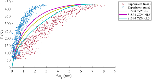
(a)

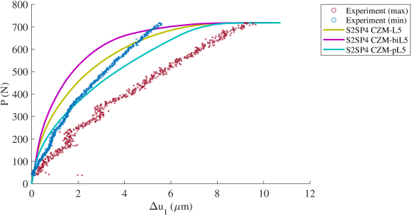
(b)

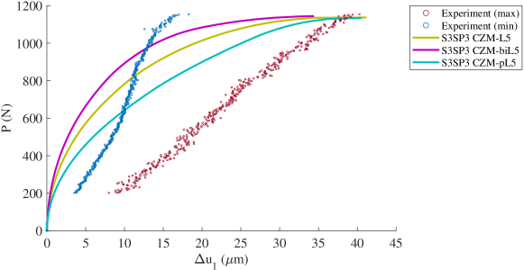
(c)

Figure 28: Simulated load-separation ($P$–$\Delta u_{1}$) curves obtained at the initial crack tips of the S1SP4, S2SP4, and S3SP3 models with based on $G^{\text{(II)}}_{\text{f,mod}}$ and $K^{\text{(II)}}_{\text{base}}$. The experimental curves for $\Delta u_{\text{max}}$ and $\Delta u_{\text{min}}$ at $x=0$ in Fig. 27 were reproduced here for comparison. (a) S1SP4 model. (b) S2SP4 model. (c) S3SP3 model.

The $P$–$\Delta u_{\text{1}}$ curves of the S1SP4, S2SP4, and S3SP3 models were initially obtained from the CZM parameters based on $K^{\text{(II)}}_{\text{base}}$ and $G^{\text{(II)}}_{\text{f,mod}}$ (see Tables 8, 10 and 13, respectively) which showed excellent agreement with the experimental $P$–$\delta$ curves. The $P$–$\Delta u_{\text{1}}$ curves of the S1SP4, S2SP4, and S3SP3 models are presented in Fig. 28. These CZM parameters did not make a notable difference in the $P$–$\delta$ curves but led to distinctive $P$–$\Delta u_{\text{1}}$ curves. For the S1SP4 model (see Fig. 28a), for example, the bilinear softening law (S1SP4 CZM biL-5) resulted in slower separation evolution than the other two cases, while separation developed quickly in the plateau-linear softening case (S1SP4 CZM pL-5). This phenomenon could occur because the linear and bilinear softening cases were given higher $\tau_{\text{f}}$ values than the plateau-linear softening case for the given $\Delta u_{\text{f}}$ and $G^{\text{(II)}}_{\text{f}}$ values. All three $P$–$\Delta u$ curves of the S1SP4 model were positioned within the boundaries of the experimental $\Delta u_{\text{min}}$ and $\Delta u_{\text{max}}$ curves, following the $\Delta u_{\text{min}}$ curve mostly. The S2SP4 and S3SP3 models, on the other hand, formed their $P$–$\Delta u_{\text{1}}$ curves on the outside of the experimental $\Delta u_{\text{min}}$ boundary and thus showed significantly stronger traction levels compared to the experimental data continuously up to the experimental $P_{\text{max}}$. The separation progression in these models was slower than the experimental $\Delta u_{\text{min}}$ case at the low load level but was accelerated between the mid and high load levels to meet $\Delta u_{\text{f}}$ at $P_{\text{max}}$.

5.2.2 $P$–$\Delta u_{\text{1}}$ curves based on $G^{\text{(II)}}_{\text{f,mod}}$ and $K^{\text{(II)}}_{\text{mod}}$

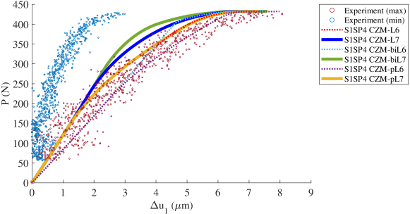
(a)

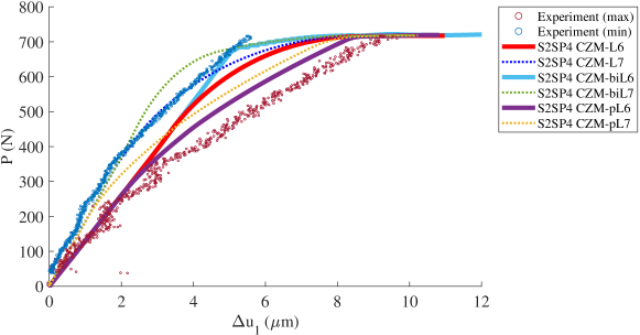
(b)

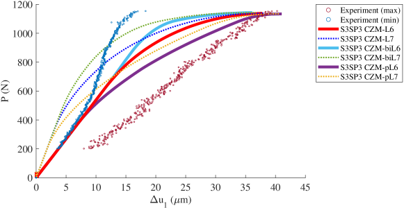
(c)

Figure 29: Simulated load-separation ($P$–$\Delta u_{1}$) curves obtained at the initial crack tips of the S1SP4, S2SP4, and S3SP3 models with $G^{\text{(II)}}_{\text{f,mod}}$ and $K^{\text{(II)}}_{\text{mod}}$. The experimental curves for $\Delta u_{\text{max}}$ and $\Delta u_{\text{min}}$ at $x=0$ in Fig. 27 were reproduced here for comparison. (a) S1SP4 model. (b) S2SP4 model. (c) S3SP3 model.

As discussed in Section 4.1, the actual separation values could be closely aligned with the experimental $\Delta u_{\text{max}}$ measurements. Therefore, the initial interlaminar stiffness $K^{\text{(II)}}$ was reduced to match simulation results with the $\Delta u_{\text{max}}$ curve in the $P$–$\Delta u_{\text{max}}$ space. The simulation results with the calibrated $K^{\text{(II)}}$ values are illustrated in Fig. 29. For the S1SP4 model, $K^{\text{(II)}}$ could not get lower than $5\times 10^{4}$ MPa/mm to incorporate the $\Delta u_{\text{f}}$ and $G^{\text{(II)}}_{\text{mod}}$ values of the S1SP4 specimen in the CZM parameters. The calibrated $K^{\text{(II)}}$ and corresponding CZM parameters are tabulated in Table 16. As shown in Fig. 29a, the plot based on $K^{\text{(II)}}=1\times 10^{5}$ MPa/mm showed good agreement with the experimental $\Delta u_{\text{max}}$ curve and thus the value was chosen as $K^{\text{(II)}}_{\text{mod}}$ for the S1SP4 model. The S2SP4 model also could not have $K^{\text{(II)}}$ smaller than $5\times 10^{4}$ MPa/mm as shown in Table 17. In contrast to the S1SP4 case, the S2SP4 model with $K^{\text{(II)}}=5\times 10^{4}$ MPa/mm performed better in the $P$–$\Delta u_{\text{max}}$ space as shown in Fig. 29b and thus adopted the value as $K^{\text{(II)}}_{\text{mod}}$. The plateau-linear softening case (S2SP4 CZM-pL6) made a good agreement with the $\Delta u_{\text{max}}$ curve, while the other two cases (S2SP4 CZM-L6 and biL6) showed slower separation development than the $\Delta u_{\text{max}}$ case, still staying within the boundaries of the experimental $\Delta u_{\text{min}}$ and $\Delta u_{\text{max}}$ curves. Lastly, the large $\Delta u_{\text{f}}$ value of the S3SP3 specimen allowed $5\times 10^{3}$ MPa/mm to be the minimum value of calibrated $K^{\text{(II)}}$ for the S3SP3 model as tabulated in Table 18. Only the $P$–$\Delta u_{\text{1}}$ curves obtained from the minimum value stayed within the experimental boundaries and thus the value was chosen as $K^{\text{(II)}}_{\text{mod}}$ for the model. The three curves followed the $\Delta u_{\text{min}}$ curve in the beginning but met the $\Delta u_{\text{max}}$ curve at $P_{\text{max}}$ with accelerated separation progression between the mid and high load levels. It needs to be noted that the $P$–$\Delta u_{\text{1}}$ curves of the three models based on the selected $K^{\text{(II)}}_{\text{mod}}$ values were plotted with thicker lines in Fig. 29.

5.3 Simulation results based on $K^{\text{(II)}}_{\text{mod}}$

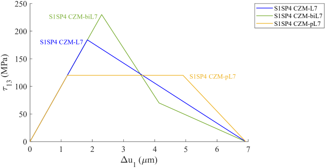
(a)

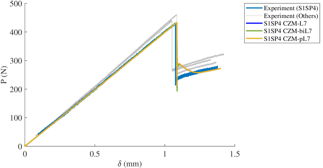
(b)

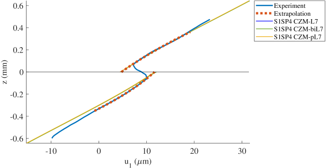
(c)

Figure 30: Traction-separation laws and simulation results of the S1SP4 model based on $G^{\text{(II)}}_{\text{f,mod}}$ and $K^{\text{(II)}}_{\text{mod}}$. (a) Traction-separation ($\tau_{\text{13}}$–$\Delta u_{\text{1}}$) laws adopted in the model. The parameters are tabulated in Table 16. (b) Load-displacement ($P$–$\delta$) curves simulated using the S1SP4 model with the $\tau_{\text{13}}$–$\Delta u_{\text{1}}$ laws shown in (a). The experimental curves in Fig. 6a were reproduced here for comparison. (c) In-plane displacement $u_{1}$ variation through the thickness at the initial crack tip under $P_{\text{max}}$. The shifted experimental curve in Fig. 20c was reproduced here for comparison.

The simulation result of the S1SP4 model based on $G^{\text{(II)}}_{\text{f,mod}}$ and $K^{\text{(II)}}_{\text{mod}}$ is illustrated in Fig. 30. The traction-separation laws in Fig. 30a were drawn based on the CZM parameters shown in Table 16. The model showed excellent agreement with the experimental $P$–$\delta$ curve as shown in Fig. 30b. The error was $0.35$–$0.80\%$ as tabulated in Table 16. The $P$–$\delta$ curves (i.e., the global behavior) of the model were almost identical to the ones based on $K^{\text{(II)}}_{\text{base}}$ shown in Fig. 22b. The in-plane displacement variation through the thickness of the model showed a good agreement with the shifted experimental curve as shown in Fig. 30c. The $u_{\text{1}}$ curves were also almost identical to the corresponding ones based on $K^{\text{(II)}}_{\text{base}}$ shown in Fig. 22c.

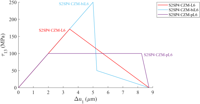
(a)

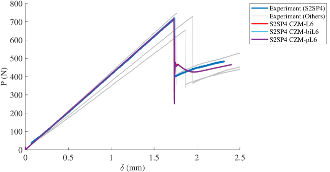
(b)

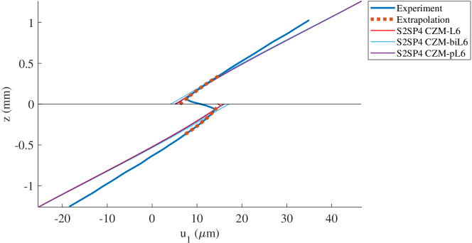
(c)

Figure 31: Traction-separation laws and simulation results of the S2SP4 model based on $G^{\text{(II)}}_{\text{f,mod}}$ and $K^{\text{(II)}}_{\text{mod}}$. (a) Traction-separation ($\tau_{\text{13}}$–$\Delta u_{\text{1}}$) laws adopted in the model. The parameters are tabulated in Table 17. (b) Load-displacement ($P$–$\delta$) curves simulated using the S2SP4 model with the $\tau_{\text{13}}$–$\Delta u_{\text{1}}$ laws shown in (a). The experimental curves in Fig. 6b were reproduced here for comparison. (c) In-plane displacement $u_{1}$ variation through the thickness at the initial crack tip under $P_{\text{max}}$. The shifted experimental curve in Fig. 23c was reproduced here for comparison.

In Fig. 31, the simulation result of the S2SP4 model based on $G^{\text{(II)}}_{\text{f,mod}}$ and $K^{\text{(II)}}_{\text{mod}}$ is presented. The CZM parameters are tabulated in Table 17 and the corresponding traction-separation laws are illustrated in Fig. 31a. As shown in Fig. 31b, the $P$–$\delta$ curves of the model made excellent agreement with the experimental one showing small errors between $-0.23$ and $0.61\%$ (see Table 17). The $u_{\text{1}}$ curves of the model in Fig. 31c were almost identical to the corresponding ones based on $K^{\text{(II)}}_{\text{base}}$ shown in Fig. 24c.

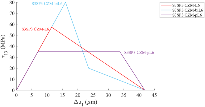
(a)

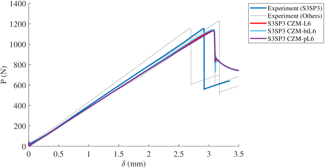
(b)

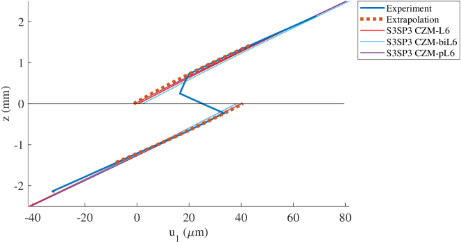
(c)

Figure 32: Traction-separation laws and simulation results of the S3SP3 model based on $G^{\text{(II)}}_{\text{f,mod}}$ and $K^{\text{(II)}}_{\text{mod}}$. (a) Traction-separation ($\tau_{\text{13}}$–$\Delta u_{\text{1}}$) laws adopted in the model. The parameters are tabulated in Table 18. (b) Load-displacement ($P$–$\delta$) curves simulated using the S3SP3 model with the $\tau_{\text{13}}$–$\Delta u_{\text{1}}$ laws shown in (a). The experimental curves in Fig. 6c were reproduced here for comparison. (c) In-plane displacement $u_{1}$ variation through the thickness at the initial crack tip under $P_{\text{max}}$. The shifted experimental curve in Fig. 25c was reproduced here for comparison.

Lastly, Fig. 32 shows the simulation result of the S3SP3 model based on $G^{\text{(II)}}_{\text{f,mod}}$ and $K^{\text{(II)}}_{\text{mod}}$. The CZM parameter sets in Table 18 led to the three traction-separation laws in Fig. 32a. The simulation result showed reasonable agreement with the experimental $P$–$\delta$ curve as shown in Fig. 32b. The error was between $-0.99$ and $-1.79\%$ as tabulated in Table 18, which was similar to the corresponding case based on $K^{\text{(II)}}_{\text{base}}$. A slightly larger softening of the stiffness, however, was observed in the $K^{\text{(II)}}_{\text{mod}}$-based curves compared to the $K^{\text{(II)}}_{\text{base}}$ cases. This phenomenon could be attributed to the significant reduction in the initial interlaminar stiffness of the model; to be specific, $K^{\text{(II)}}_{\text{mod}}=0.005K^{\text{(II)}}_{\text{base}}$ for the S3SP3 model. The $u_{\text{1}}$ curves of the model made excellent agreement with the shifted experimental curve as shown in Fig. 32c.

5.4 Discussions

The impact of the initial interlaminar stiffness $K^{\text{(II)}}$ was well captured in the $P$–$\Delta u_{\text{1}}$ spaces. Smaller $K^{\text{(II)}}$ values were needed for larger sizes to match the experimental $P$–$\Delta u_{\text{1}}$ curves. To be specific, the modified $K^{\text{(II)}}$ was $K^{\text{(II)}}_{\text{mod}}=0.1K^{\text{(II)}}_{\text{base}}$ for the S1SP4 model, $K^{\text{(II)}}_{\text{mod}}=0.05K^{\text{(II)}}_{\text{base}}$ for the S2SP4 model, and $K^{\text{(II)}}_{\text{mod}}=0.005K^{\text{(II)}}_{\text{base}}$ for the S3SP3 model. These reductions in $K^{\text{(II)}}$ did not lead to a notable change in the global behaviors of the models. This would imply that the global behaviors could significantly be dictated by neither $K^{\text{(II)}}$ nor softening types but by $G^{\text{(II)}}_{\text{f}}$. It needs to be noted that $K^{\text{(II)}}$ should be a material property as a traction-separation parameter. Therefore, a single value of $K^{\text{(II)}}$ should exist for a given material satisfying global-local validation in the form of a $P$–$\Delta u_{\text{1}}$ curve. To address this issue, other fracture mechanisms like plastic dissipation will be considered in future work and their impacts on separation development will be investigated in the $P$–$\Delta u_{\text{1}}$ space.

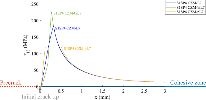
(a)

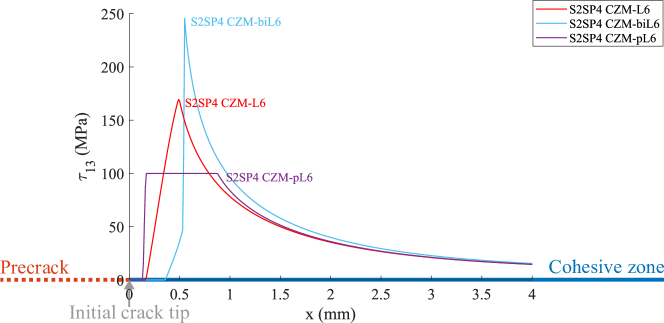
(b)

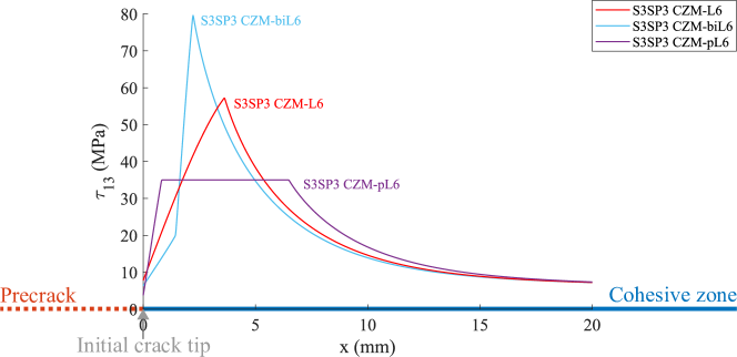
(c)

Figure 33: Distribution of traction $\tau_{\text{13}}$ between the upper and lower parts at $P_{\text{max}}$ simulated using the traction-separation laws based on $G^{\text{(II)}}_{\text{f,mod}}$ and $K^{\text{(II)}}_{\text{mod}}$. (a) S1SP4 model. (b) S2SP4 model. (c) S3SP3 model.

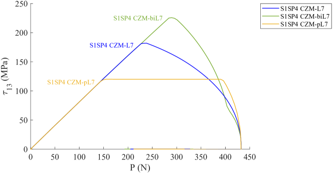
(a)

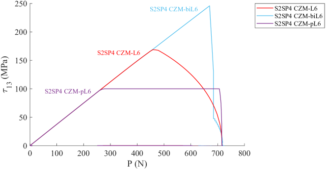
(b)

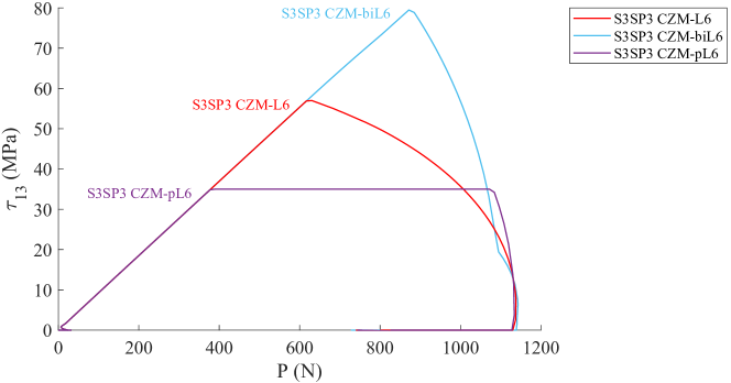
(c)

Figure 34: Load-traction ($P$–$\tau_{\text{13}}$) curves simulated using the traction-separation laws based on $G^{\text{(II)}}_{\text{f,mod}}$ and $K^{\text{(II)}}_{\text{mod}}$. (a) S1SP4 model. (b) S2SP4 model. (c) S3SP3 model.

Another interesting phenomenon was observed from the distribution of traction $\tau_{\text{13}}$ between the upper and lower parts of the models at $P_{\text{max}}$ as shown in Fig. 33. The S1SP4 model (see Fig. 33a) experienced complete separation (i.e., zero traction) at the initial crack tip marginally prior to $P_{\text{max}}$ for all three softening types. In the S2SP4 model (see Fig. 33b), the precrack propagated from the initial crack tip along the cohesive zone before $P_{\text{max}}$ was reached. The early damage propagation was observed in all the three softening types, while the propagation magnitude was more significant in the bilinear softening type than in the other types. This phenomenon possibly contributed to the discrepancy between the $u_{\text{1}}$ curves of the specimen and the model shown in Fig. 34. The S3SP3 model, on the contrary, showed partial CZM development at $P_{\text{max}}$ for all the softening laws. Complete separation at the initial crack tip was observed on the postpeak $P$–$\delta$ curves. The snapdown of the $P$–$\delta$ curves followed immediately after complete separation occurred at the initial crack tip.

Finally, additional global-local synchronization was made using $P$–$\tau_{\text{13}}$ plots as shown in Fig. 34. It should be noted that softening (or fracture process) could be initiated at low load levels depending on softening types. For the plateau-linear softening cases, the initial crack tip was subject to softening at 154.3 N ($0.36P_{\text{max}}$), 278.7 N ($0.39P_{\text{max}}$), and 390.8 N ($0.34P_{\text{max}}$) for the S1SP4, S2SP4, and S3SP3 models, respectively. Using Eq. 5 based on the compliance calibration method, these load values give $13.0$, $15.2$, and $11.6$ $\%G_{\text{Q}}$ for the S1SP4, S2SP4, and S3SP3 specimens, respectively. The ASTM manual specifies that maximum loads applied for compliance calibration tests should exceed $15$ $\%G_{\text{Q}}$ as shown in Eq. 4. For certain materials, however, a fracture process could be initiated by releasing fracture energies during compliance calibration tests prior to actual fracture tests depending on their traction-separation law types. Therefore, this issue might require more investigation for the broadly used test method.

6 Conclusions

The work herein was focused on developing an experimental framework to characterize high-fidelity damage models for composites in the form of cohesive zone models (CZM) based on traction-separation laws. This paper presented part of the work related to solving a specific challenge problem, mode-II interlaminar fracture in scaled End-Notched Flexure (ENF) specimens under three-point bending.

The experimental data revealed the limitation of the compliance calibration method in the ASTM manual which is widely used based on Linear Elastic Fracture Mechanics (LEFM). The method failed to estimate the fracture energy of the specimen material as a single material property value, showing an increase in the fracture energy with scaling up of the specimen dimensions. To address this issue, Bažant’s type-II size effect law was applied to the experimental data of the global fracture behaviors in the scaled specimens and a single fracture energy value was obtained. For the experimental characterization of local fracture behaviors, a through-thickness analysis of in-plane displacement was proposed and implemented using microscopic Digital Image Correlation (DIC) data. This analysis method was proposed to overcome difficulties in identifying the exact location of a fracture process zone and the impact of superficial traction induced by speckle paints. Using the proposed method, the in-plane separation magnitudes were characterized at the initial crack tips in the specimens at their maximum load levels.

For numerical modeling based on CZM, traction-separation laws were formulated for the specimen material based on the experimental measurement of the fracture energy and critical separation values. The fracture energy values were modified to match the experimental load-displacement curves; however, the CZM parameters performed well only for a single scale. Furthermore, the load-displacement curves of the models were insensitive to changes in initial interface stiffness values and softening types. To overcome the limitations of model validation relying on load-displacement curves, a progressive DIC analysis of separation evolution was proposed. This method was intended for experimental synchronization between global and local fracture behaviors in the load-separation space. The impact of initial interface stiffness was successfully captured using the proposed method. The calibrated stiffness values, however, showed inconsistency and decreased with an increase in geometric scales. Therefore, this phenomenon needs to be further investigated in future work by considering other potential fracture mechanisms like plastic dissipation in the vicinity of an initial crack tip. It should be noted that the proposed methods were applied to a specific mode-II interlaminar fracture process in laminated carbon/epoxy composites; however, this method would be applicable to the other fracture modes and materials.

Based on the experimental and simulation results herein, future work will be focused on characterizing a single traction-separation law for the specimen material. It was observed from the experimental data that the separation values at the maximum loads increased with an increase in the scaling factor. Furthermore, higher fracture energies (but still smaller than the fracture energy obtained from the size effect analysis) were needed for the models to match the global behaviors of the larger specimens. Therefore, smaller energy would be released in a smaller specimen under its maximum load due to partial CZM development at a lower separation level. In future work, more efforts will be made to characterize corresponding traction values at the maximum loads for the piecewise characterization of the exact traction-separation law shape.

7 Acknowledgments

The authors gratefully acknowledge the support of the Air Force Office of Scientific Research (Grant numbers: FA9550-19-1-0031 and ARCTOS 162643-19-26-C1) and the Air Force Research Laboratory’s Structural Sciences Center at Wright-Patterson Air Force Base.

8 Data availability

The raw/processed data required to reproduce these findings cannot be shared at this time due to technical limitations.

Table 1: Lamina/laminate mechanical properties of the Toray T700G/2510 carbon/epoxy prepreg system [52]

Property		Value
$0^{\circ}$ tensile modulus, ${E_{\text{1t}}}$ (GPa)		$125$
$90^{\circ}$ tensile modulus, ${E_{\text{2t}}}$ (GPa)		$8.41$
In-plane shear modulus, ${G_{\text{12}}}$ (GPa)		$4.23$
Poisson’s ratio, ${\nu_{\text{12}}}$ (GPa)		$0.31$

Table 2: Geometric dimensions of the scaled ENF specimens

Dimension		Size 1		Size 2		Size 3
Gauge length, ${L}$ (mm)		$36$		$72$		$144$
Nominal thickness, ${h}$ (mm)		$1.25$		$2.5$		$5.0$
Nominal width, ${b}$ (mm)		$25$		$25$		$25$
Initial crack length, ${a_{\text{0}}}$ (mm)		$10$		$20$		$40$
Compliance crack length, ${a_{\text{1}}}$ (mm)		$7$		$15$		$30$
Compliance crack length, ${a_{\text{2}}}$ (mm)		$13$		$25$		$50$

Table 3: Labels and actual dimensions of the specimens

Size	Specimen	Label	$\boldsymbol{b}$ (mm)	$\boldsymbol{h}$ (mm)
1	1	S1SP1	25.7	1.30
	2	S1SP2	25.4	1.32
	3	S1SP3	25.4	1.29
	4	S1SP4	23.1	1.31
2	1	S2SP1	25.0	2.46
	2	S2SP2	24.0	2.50
	3	S2SP3	27.0	2.54
	4	S2SP4	25.8	2.54
3	1	S3SP1	25.8	4.98
	2	S3SP2	26.4	4.95
	3	S3SP3	24.8	5.01
	4	S3SP4	26.7	5.04

Table 4: Compliance calibration test data of the specimens

Label	$\boldsymbol{C}_{0}$ / $\boldsymbol{C}_{1}$ / $\boldsymbol{C}_{2}$	$\boldsymbol{A}$	$\boldsymbol{m}$	$\boldsymbol{R}^{2}$
	(mm/N)	(mm/N)	(1/$\text{mm}^{2}\text{N}$)
S1SP1	2.429 / 2.046 / 3.091$\times 10^{-3}$	1.858$\times 10^{-3}$	5.626$\times 10^{-7}$	0.9998
S1SP2	2.389 / 1.995 / 2.664$\times 10^{-3}$	1.943$\times 10^{-3}$	3.448$\times 10^{-7}$	0.9295
S1SP3	2.397 / 2.001 / 2.811$\times 10^{-3}$	1.900$\times 10^{-3}$	4.259$\times 10^{-7}$	0.9766
S1SP4	2.523 / 2.246 / 3.048$\times 10^{-3}$	2.094$\times 10^{-3}$	4.333$\times 10^{-7}$	0.9999
S2SP1	2.881 / 2.498 / 3.437$\times 10^{-3}$	2.252$\times 10^{-3}$	7.625$\times 10^{-8}$	0.9988
S2SP2	2.682 / 2.377 / 3.351$\times 10^{-3}$	2.081$\times 10^{-3}$	8.030$\times 10^{-8}$	0.9949
S2SP3	2.361 / 2.077 / 2.857$\times 10^{-3}$	1.857$\times 10^{-3}$	6.383$\times 10^{-8}$	0.9998
S2SP4	2.435 / 2.163 / 3.024$\times 10^{-3}$	1.902$\times 10^{-3}$	7.093$\times 10^{-8}$	0.9952
S3SP1	2.637 / 2.249 / 2.842$\times 10^{-3}$	2.160$\times 10^{-3}$	5.779$\times 10^{-9}$	0.9034
S3SP2	2.511 / 2.191 / 2.947$\times 10^{-3}$	1.999$\times 10^{-3}$	7.658$\times 10^{-9}$	0.9973
S3SP3	2.498 / 2.180 / 2.977$\times 10^{-3}$	1.968$\times 10^{-3}$	8.108$\times 10^{-9}$	0.9994
S3SP4	2.309 / 2.049 / 2.771$\times 10^{-3}$	1.844$\times 10^{-3}$	7.386$\times 10^{-9}$	0.9996

Table 5: Actual dimensions, maximum loads $P_{\text{max}}$, effective flexural modulus $\bar{E}_{\text{1f}}$, LEFM fracture energies $G_{\text{f,LEFM}}^{\text{(II)}}$ and nominal strengths $\sigma_{\text{Nc}}$ of the specimens

Label	$\boldsymbol{P_{\text{max}}}$	$\boldsymbol{\bar{E}_{\text{1f}}}$	$\boldsymbol{\%G_{\text{Q,1}}^{\text{(II)}}}$ / $\boldsymbol{\%G_{\text{Q,2}}^{\text{(II)}}}$	$\boldsymbol{G_{\text{f,LEFM}}^{\text{(II)}}}$	$\boldsymbol{\sigma_{\text{Nc}}}$
	(N)	(GPa)	($\%$)	(N/mm)	(MPa)
S1SP1	439	110.1	16.02 / 16.56	0.63	13.10
S1SP2	443	102.6	15.82 / 16.11	0.40	13.18
S1SP3	462	112.0	14.55 / 15.11	0.54	14.07
S1SP4	431	107.7	16.69 / 17.11	0.52	14.23
S2SP1	656	112.0	21.25 / 21.43	0.79	10.69
S2SP2	731	119.8	16.96 / 17.42	1.07	12.19
S2SP3	748	114.1	16.33 / 16.61	0.79	10.92
S2SP4	719	115.8	17.65 / 17.85	0.85	10.95
S3SP1	1141	108.4	15.74 / 14.78	0.70	8.88
S3SP2	1233	117.0	19.85 / 20.11	1.06	9.45
S3SP3	1154	121.2	22.62 / 22.96	1.01	9.27
S3SP4	1151	118.7	22.77 / 22.92	0.91	8.56

Table 6: Separation values $\Delta u$ and FPZ sizes estimated from the DIC analysis data

Label	$\Delta\boldsymbol{u}_{\text{max}}$ (µm)	$\Delta\boldsymbol{u}_{\text{min}}$ (µm)	FPZ size (mm)
S1SP4	6.92	2.85	2.0
S2SP4	8.75	6.06	3.0
S3SP3	41.85	17.00	22.0

Table 7: CZM parameters and simulation results of the S1SP4 model based on $G^{\text{(II)}}_{\text{f,LEFM}}$ of the S1SP4 specimen (0.52 N/mm)

CZM label	$\boldsymbol{K}^{\text{(II)}}$	$\boldsymbol{\tau}_{0}$ / $\boldsymbol{\tau}_{\text{f}}$	$\Delta\boldsymbol{u}_{0}$ / $\Delta\boldsymbol{u}_{\text{f}}$	FPZ	$\boldsymbol{P}_{\text{max}}$	Error
	(MPa/mm)	(MPa)	(µm)	(mm)	(N)	(%)
S1SP4 CZM-L1	$5\times 10^{4}$	- / 150.3	- / 6.92	0.30	387.7	$-9.96$
S1SP4 CZM-L2	$1\times 10^{5}$	- / 150.3	- / 6.92	0.42	388.0	$-9.89$
S1SP4 CZM-L3	$1\times 10^{6}$	- / 150.3	- / 6.92	0.56	388.2	$-9.83$
S1SP4 CZM-L4	$1\times 10^{7}$	- / 150.3	- / 6.92	0.61	388.3	$-9.81$
S1SP4 CZM-biL1	$5\times 10^{4}$	70 / 200	4.17 / 6.92	0.19	389.0	$-9.64$
S1SP4 CZM-biL2	$1\times 10^{5}$	70 / 200	3.48 / 6.92	0.33	388.0	$-9.89$
S1SP4 CZM-biL3	$1\times 10^{6}$	70 / 200	2.85 / 6.92	0.48	388.3	$-9.81$
S1SP4 CZM-biL4	$1\times 10^{7}$	70 / 200	2.79 / 6.92	0.53	388.4	$-9.80$
S1SP4 CZM-pL1	$5\times 10^{4}$	- / 100	5.48 / 6.92	0.50	387.4	$-10.02$
S1SP4 CZM-pL2	$1\times 10^{5}$	- / 100	4.48 / 6.92	0.60	387.8	$-9.92$
S1SP4 CZM-pL3	$1\times 10^{6}$	- / 100	3.58 / 6.92	0.74	387.8	$-9.93$
S1SP4 CZM-pL4	$1\times 10^{7}$	- / 100	3.49 / 6.92	0.76	388.0	$-9.89$

Table 8: CZM parameters and simulation results of the S1SP4 model based on $G^{\text{(II)}}_{\text{f,mod}}$ of the S1SP4 specimen (0.6375 N/mm) with $K^{\text{(II)}}_{\text{base}}$

CZM label	$\boldsymbol{K}^{\text{(II)}}$	$\boldsymbol{\tau}_{0}$ / $\boldsymbol{\tau}_{\text{f}}$	$\Delta\boldsymbol{u}_{0}$ / $\Delta\boldsymbol{u}_{\text{f}}$	FPZ	$\boldsymbol{P}_{\text{max}}$	Error
	(MPa/mm)	(MPa)	(µm)	(mm)	(N)	(%)
S1SP4 CZM-L5	$1\times 10^{6}$	- / 184.2	- / 6.92	0.50	433.0	0.56
S1SP4 CZM-biL5	$1\times 10^{6}$	70 / 230	3.51 / 6.92	0.42	433.0	0.57
S1SP4 CZM-pL5	$1\times 10^{6}$	- / 120	3.83 / 6.92	0.65	432.8	0.52

Table 9: CZM parameters and simulation results of the S2SP4 model based on $G^{\text{(II)}}_{\text{f,LEFM}}$ of the S2SP4 specimen (0.85 N/mm)

CZM label	$\boldsymbol{K}^{\text{(II)}}$	$\boldsymbol{\tau}_{0}$ / $\boldsymbol{\tau}_{\text{f}}$	$\Delta\boldsymbol{u}_{0}$ / $\Delta\boldsymbol{u}_{\text{f}}$	FPZ	$\boldsymbol{P}_{\text{max}}$	Error
	(MPa/mm)	(MPa)	(µm)	(mm)	(N)	(%)
S2SP4 CZM-L1	$5\times 10^{4}$	- / 194.3	- / 8.75	0.46	765.9	6.49
S2SP4 CZM-L2	$1\times 10^{5}$	- / 194.3	- / 8.75	0.54	766.4	6.57
S2SP4 CZM-L3	$1\times 10^{6}$	- / 194.3	- / 8.75	0.69	766.8	6.62
S2SP4 CZM-L4	$1\times 10^{7}$	- / 194.3	- / 8.75	0.75	767.1	6.67
S2SP4 CZM-biL1	$5\times 10^{4}$	70 / 250	5.75 / 8.75	0.34	767.9	6.78
S2SP4 CZM-biL2	$1\times 10^{5}$	70 / 250	5.05 / 8.75	0.50	766.6	6.59
S2SP4 CZM-biL3	$1\times 10^{6}$	70 / 250	4.42 / 8.75	0.66	767.0	6.66
S2SP4 CZM-biL4	$1\times 10^{7}$	70 / 250	4.36 / 8.75	0.64	767.0	6.65
S2SP4 CZM-pL1	$5\times 10^{4}$	- / 120	7.82 / 8.75	0.64	766.9	6.64
S2SP4 CZM-pL2	$1\times 10^{5}$	- / 120	6.62 / 8.75	0.86	766.5	6.58
S2SP4 CZM-pL3	$1\times 10^{6}$	- / 120	5.54 / 8.75	1.00	767.0	6.66
S2SP4 CZM-pL4	$1\times 10^{7}$	- / 120	5.43 / 8.75	0.99	767.0	6.65

Table 10: CZM parameters and simulation results of the S2SP4 model based on $G^{\text{(II)}}_{\text{f,mod}}$ of the S2SP4 specimen (0.75 N/mm) with $K^{\text{(II)}}_{\text{base}}$

CZM label	$\boldsymbol{K}^{\text{(II)}}$	$\boldsymbol{\tau}_{0}$ / $\boldsymbol{\tau}_{\text{f}}$	$\Delta\boldsymbol{u}_{0}$ / $\Delta\boldsymbol{u}_{\text{f}}$	FPZ	$\boldsymbol{P}_{\text{max}}$	Error
	(MPa/mm)	(MPa)	(µm)	(mm)	(N)	(%)
S2SP4 CZM-L5	$1\times 10^{6}$	- / 171.4	- / 8.75	0.81	718.1	$-0.15$
S2SP4 CZM-biL5	$1\times 10^{6}$	50 / 250	4.30 / 8.75	0.65	718.5	$-0.09$
S2SP4 CZM-pL5	$1\times 10^{6}$	- / 100	6.30 / 8.75	1.18	718.1	$-0.15$

Table 11: CZM parameters and simulation results of the S2SP4 model based on $G^{\text{(II)}}_{\text{f,mod}}$ of the S1SP4 specimen (0.6375 N/mm) with $K^{\text{(II)}}_{\text{base}}$

CZM label	$\boldsymbol{K}^{\text{(II)}}$	$\boldsymbol{\tau}_{0}$ / $\boldsymbol{\tau}_{\text{f}}$	$\Delta\boldsymbol{u}_{0}$ / $\Delta\boldsymbol{u}_{\text{f}}$	FPZ	$\boldsymbol{P}_{\text{max}}$	Error
	(MPa/mm)	(MPa)	(µm)	(mm)	(N)	(%)
S1SP4 CZM-L5	$1\times 10^{6}$	- / 184.2	- / 6.92	0.69	664.4	$-7.62$
S1SP4 CZM-biL5	$1\times 10^{6}$	70 / 230	3.51 / 6.92	0.61	664.8	$-7.56$
S1SP4 CZM-pL5	$1\times 10^{6}$	- / 120	3.83 / 6.92	0.88	664.7	$-7.58$

Table 12: CZM parameters and simulation results of the S3SP3 model based on $G^{\text{(II)}}_{\text{f,LEFM}}$ of the S3SP3 specimen ($1.01$ N/mm)

CZM label	$\boldsymbol{K}^{\text{(II)}}$	$\boldsymbol{\tau}_{0}$ / $\boldsymbol{\tau}_{\text{f}}$	$\Delta\boldsymbol{u}_{0}$ / $\Delta\boldsymbol{u}_{\text{f}}$	FPZ	$\boldsymbol{P}_{\text{max}}$	Error
	(MPa/mm)	(MPa)	(µm)	(mm)	(N)	(%)
S3SP3 CZM-L1	$5\times 10^{4}$	- / 48.3	- / 41.85	6.48	1033.1	$-10.51$
S3SP3 CZM-L2	$1\times 10^{5}$	- / 48.3	- / 41.85	6.68	1033.3	$-10.50$
S3SP3 CZM-L3	$1\times 10^{6}$	- / 48.3	- / 41.85	6.88	1033.4	$-10.49$
S3SP3 CZM-L4	$1\times 10^{7}$	- / 48.3	- / 41.85	7.12	1033.4	$-10.49$
S3SP3 CZM-biL1	$5\times 10^{4}$	20 / 80	15.19 / 41.85	4.72	1038.7	$-10.03$
S3SP3 CZM-biL2	$1\times 10^{5}$	20 / 80	14.99 / 41.85	4.94	1038.7	$-10.03$
S3SP3 CZM-biL3	$1\times 10^{6}$	20 / 80	14.81 / 41.85	5.18	1038.7	$-10.03$
S3SP3 CZM-biL4	$1\times 10^{7}$	20 / 80	14.79 / 41.85	5.20	1038.8	$-10.02$
S3SP3 CZM-pL1	$5\times 10^{4}$	- / 30	26.08 / 41.85	9.08	1029.2	$-10.85$
S3SP3 CZM-pL2	$1\times 10^{5}$	- / 30	25.78 / 41.85	9.26	1029.1	$-10.86$
S3SP3 CZM-pL3	$1\times 10^{6}$	- / 30	25.51 / 41.85	9.48	1028.9	$-10.87$
S3SP3 CZM-pL4	$1\times 10^{7}$	- / 30	25.49 / 41.85	9.50	1029.6	$-10.82$

Table 13: CZM parameters and simulation results of the S3SP3 model based on $G^{\text{(II)}}_{\text{f,mod}}$ of the S3SP3 specimen (1.20 N/mm) with $K^{\text{(II)}}_{\text{base}}$

CZM label	$\boldsymbol{K}^{\text{(II)}}$	$\boldsymbol{\tau}_{0}$ / $\boldsymbol{\tau}_{\text{f}}$	$\Delta\boldsymbol{u}_{0}$ / $\Delta\boldsymbol{u}_{\text{f}}$	FPZ	$\boldsymbol{P}_{\text{max}}$	Error
	(MPa/mm)	(MPa)	(µm)	(mm)	(N)	(%)
S3SP3 CZM-L5	$1\times 10^{6}$	- / 57.3	- / 41.85	6.70	1137.1	$-1.51$
S3SP3 CZM-biL5	$1\times 10^{6}$	20 / 80	19.56 / 41.85	4.80	1143.9	$-0.91$
S3SP3 CZM-pL5	$1\times 10^{6}$	- / 35	26.76 / 41.85	8.64	1134.69	$-1.71$

Table 14: CZM parameters and simulation results of the S3SP3 model based on $G^{\text{(II)}}_{\text{f,mod}}$ of the S1SP4 specimen (0.6375 N/mm) with $K^{\text{(II)}}_{\text{base}}$

CZM label	$\boldsymbol{K}^{\text{(II)}}$	$\boldsymbol{\tau}_{0}$ / $\boldsymbol{\tau}_{\text{f}}$	$\Delta\boldsymbol{u}_{0}$ / $\Delta\boldsymbol{u}_{\text{f}}$	FPZ	$\boldsymbol{P}_{\text{max}}$	Error
	(MPa/mm)	(MPa)	(µm)	(mm)	(N)	(%)
S1SP4 CZM-L5	$1\times 10^{6}$	- / 184.2	- / 6.92	0.90	900.4	$-22.01$
S1SP4 CZM-biL5	$1\times 10^{6}$	70 / 230	3.51 / 6.92	1.34	900.5	$-22.00$
S1SP4 CZM-pL5	$1\times 10^{6}$	- / 120	3.83 / 6.92	1.14	900.3	$-22.02$

Table 15: CZM parameters and simulation results of the S3SP3 model based on $G^{\text{(II)}}_{\text{f,mod}}$ of the S2SP4 specimen (0.75 N/mm) with $K^{\text{(II)}}_{\text{base}}$

CZM label	$\boldsymbol{K}^{\text{(II)}}$	$\boldsymbol{\tau}_{0}$ / $\boldsymbol{\tau}_{\text{f}}$	$\Delta\boldsymbol{u}_{0}$ / $\Delta\boldsymbol{u}_{\text{f}}$	FPZ	$\boldsymbol{P}_{\text{max}}$	Error
	(MPa/mm)	(MPa)	(µm)	(mm)	(N)	(%)
S2SP4 CZM-L5	$1\times 10^{6}$	- / 171.4	- / 8.75	1.12	974.0	$-15.63$
S2SP4 CZM-biL5	$1\times 10^{6}$	50 / 250	4.30 / 8.75	1.18	974.5	$-15.59$
S2SP4 CZM-pL5	$1\times 10^{6}$	- / 100	6.30 / 8.75	1.42	974.5	$-15.59$

Table 16: CZM parameters and simulation results of the S1SP4 model based on $G^{\text{(II)}}_{\text{f,mod}}$ of the S1SP4 specimen (0.6375 N/mm) with the modified $K^{\text{(II)}}$

CZM label	$\boldsymbol{K}^{\text{(II)}}$	$\boldsymbol{\tau}_{0}$ / $\boldsymbol{\tau}_{\text{f}}$	$\Delta\boldsymbol{u}_{0}$ / $\Delta\boldsymbol{u}_{\text{f}}$	FPZ	$\boldsymbol{P}_{\text{max}}$	Error
	(MPa/mm)	(MPa)	(µm)	(mm)	(N)	(%)
S1SP4 CZM-L6	$5\times 10^{4}$	- / 184.2	- / 6.92	0.19	432.2	0.38
S1SP4 CZM-L7	$1\times 10^{5}$	- / 184.2	- / 6.92	0.33	432.5	0.44
S1SP4 CZM-biL6	$5\times 10^{4}$	70 / 230	4.84 / 6.92	0.14	434.0	0.80
S1SP4 CZM-biL7	$1\times 10^{5}$	70 / 230	4.14 / 6.92	0.28	432.6	0.47
S1SP4 CZM-pL6	$5\times 10^{4}$	- / 120	6.11 / 6.92	0.42	432.0	0.35
S1SP4 CZM-pL7	$1\times 10^{5}$	- / 120	4.91 / 6.92	0.51	432.5	0.46

Table 17: CZM parameters and simulation results of the S2SP4 model based on $G^{\text{(II)}}_{\text{f,mod}}$ of the S2SP4 specimen (0.75 N/mm) with the modified $K^{\text{(II)}}$

CZM label	$\boldsymbol{K}^{\text{(II)}}$	$\boldsymbol{\tau}_{0}$ / $\boldsymbol{\tau}_{\text{f}}$	$\Delta\boldsymbol{u}_{0}$ / $\Delta\boldsymbol{u}_{\text{f}}$	FPZ	$\boldsymbol{P}_{\text{max}}$	Error
	(MPa/mm)	(MPa)	(µm)	(mm)	(N)	(%)
S2SP4 CZM-L6	$5\times 10^{4}$	- / 171.4	- / 8.75	0.49	717.5	$-0.23$
S2SP4 CZM-L7	$1\times 10^{5}$	- / 171.4	- / 8.75	0.58	717.7	$-0.21$
S2SP4 CZM-biL6	$5\times 10^{4}$	50 / 250	5.25 / 8.75	0.55	723.5	0.61
S2SP4 CZM-biL7	$1\times 10^{5}$	50 / 250	4.75 / 8.75	0.44	718.5	$-0.09$
S2SP4 CZM-pL6	$5\times 10^{4}$	- / 100	8.25 / 8.75	0.87	719.4	0.04
S2SP4 CZM-pL7	$1\times 10^{5}$	- / 100	7.25 / 8.75	0.97	717.9	$-0.18$

Table 18: CZM parameters and simulation results of the S3SP3 model based on $G^{\text{(II)}}_{\text{f,mod}}$ of the S3SP3 specimen (1.20 N/mm) with the modified $K^{\text{(II)}}$

CZM label	$\boldsymbol{K}^{\text{(II)}}$	$\boldsymbol{\tau}_{0}$ / $\boldsymbol{\tau}_{\text{f}}$	$\Delta\boldsymbol{u}_{0}$ / $\Delta\boldsymbol{u}_{\text{f}}$	FPZ	$\boldsymbol{P}_{\text{max}}$	Error
	(MPa/mm)	(MPa)	(µm)	(mm)	(N)	(%)
S3SP3 CZM-L6	$5\times 10^{3}$	- / 57.3	- / 41.85	3.62	1138.0	$-1.43$
S3SP3 CZM-L7	$2\times 10^{4}$	- / 57.3	- / 41.85	5.44	1138.6	$-1.37$
S3SP3 CZM-biL6	$5\times 10^{3}$	20 / 80	23.54 / 41.85	2.22	1143.0	$-0.99$
S3SP3 CZM-biL7	$2\times 10^{4}$	20 / 80	20.54 / 41.85	4.20	1143.0	$-1.00$
S3SP3 CZM-pL6	$5\times 10^{3}$	- / 35	33.72 / 41.85	6.48	1133.8	$-1.79$
S3SP3 CZM-pL7	$2\times 10^{4}$	- / 35	28.47 / 41.85	7.94	1134.5	$-1.73$

(a)

(b)

(c)

Figure 1: Material types and related fracture behaviors. Stress distributions along FPZs are illustrated in the form of $\sigma$ curves. Yield and fracture loads are represented as $P_{\text{Y}}$ and $P_{\text{cr}}$, respectively, while crack opening displacements are described with $w$. (a) Brittle material. (b) Ductile material. (c) Quasibrittle material. This illustration was made based on the work of Bažant and Le [2].

Figure 2: Schematics of the multiple physics elements and couplings for high-speed aircraft under aerothermodynamic loading [29].

Figure 3: Schematics of the scaled ENF specimens. The thickness, gauge length, width, and initial crack length of the Size-3 specimen are represented by $h$, $L$, $b$, and $a_{0}$, respectively. The geometric dimensions of the specimens are shown in Table 2.

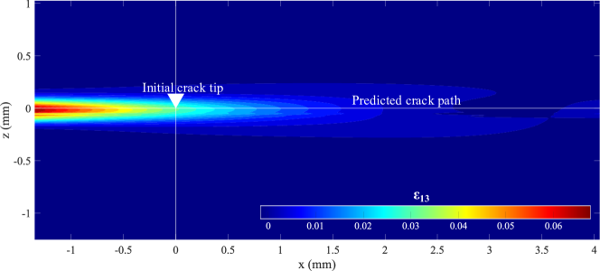
(a)

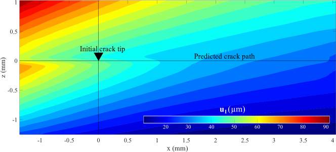
(b)

Figure 12: Microscopic DIC analysis of the S2SP4 data at $P_{\text{max}}$. The contours are presented in the undeformed configuration of the specimen where the axes $1$ and $3$ were aligned with the axes $x$ and $z$, respectively. (a) The contours of the out-of-plane shear strain $\varepsilon_{\text{13}}$ in the vicinity of the crack tip. (b) The contours of the in-plane displacement $u_{1}$ in the vicinity of the crack tip.

(a)

(b)

Figure 19: Screenshots of the Abaqus model of the S1SP4 specimen with descriptions. The model is presented here in its undeformed configuration where the axes $1$ and $3$ are aligned with the axes $x$ and $z$, respectively. (a) The assembly of the following parts: the upper and lower beam parts and loading and supporting rollers. (b) The mesh of the elements in the vicinity of the initial crack tip on the upper beam part.

(a)

(b)

(a)

(b)

(c)

Figure 23: Traction-separation laws and simulation results of the S2SP4 model based on $G^{\text{(II)}}_{\text{f,LEFM}}$. (a) Traction-separation ($\tau_{\text{13}}$–$\Delta u_{\text{1}}$) laws adopted in the model. The parameters are tabulated in Table 9. (b) Load-displacement ($P$–$\delta$) curves simulated using the S2SP4 model with the $\tau_{\text{13}}$–$\Delta u_{\text{1}}$ laws shown in (a). The experimental curves in Fig. 6b were reproduced here for comparison. (c) In-plane displacement $u_{1}$ variation through the thickness at the initial crack tip under $P_{\text{max}}$. The experimental curve and its extrapolation in Fig. 15a were shifted here by $-37.9$ µm in the $u_{\text{1}}$ axis for comparison.

(a)

(b)

(c)

Figure 24: Traction-separation laws and simulation results of the S2SP4 model based on $G^{\text{(II)}}_{\text{f,mod}}$. (a) Traction-separation ($\tau_{\text{13}}$–$\Delta u_{\text{1}}$) laws adopted in the model. The parameters are tabulated in Table 10. (b) Load-displacement ($P$–$\delta$) curves simulated using the S2SP4 model with the $\tau_{\text{13}}$–$\Delta u_{\text{1}}$ laws shown in (a). The experimental curves in Fig. 6b were reproduced here for comparison. (c) In-plane displacement $u_{1}$ variation through the thickness at the initial crack tip under $P_{\text{max}}$. The shifted experimental curve in Fig. 23c was reproduced here for comparison.

(a)

(b)

(c)

Figure 25: Traction-separation laws and simulation results of the S3SP3 model based on $G^{\text{(II)}}_{\text{f,LEFM}}$. (a) Traction-separation ($\tau_{\text{13}}$–$\Delta u_{\text{1}}$) laws adopted in the model. The parameters are tabulated in Table 12. (b) Load-displacement ($P$–$\delta$) curves simulated using the S3SP3 model with the $\tau_{\text{13}}$–$\Delta u_{\text{1}}$ laws shown in (a). The experimental curves in Fig. 6c were reproduced here for comparison. (c) In-plane displacement $u_{1}$ variation through the thickness at the initial crack tip under $P_{\text{max}}$. The shifted experimental curve in Fig. 24c was reproduced here for comparison.

(a)

(b)

(c)

Figure 26: Traction-separation laws and simulation results of the S3SP3 model based on $G^{\text{(II)}}_{\text{f,mod}}$. (a) Traction-separation ($\tau_{\text{13}}$–$\Delta u_{\text{1}}$) laws adopted in the model. The parameters are tabulated in Table 13. (b) Load-displacement ($P$–$\delta$) curves simulated using the S3SP3 model with the $\tau_{\text{13}}$–$\Delta u_{\text{1}}$ laws shown in (a). The experimental curves in Fig. 6c were reproduced here for comparison. (c) In-plane displacement $u_{1}$ variation through the thickness at the initial crack tip under $P_{\text{max}}$. The shifted experimental curve in Fig. 25c was reproduced here for comparison.

(a)

(b)

(c)

Figure 27: Experimental load-separation ($P$–$\Delta u_{1}$) curves. The curves were plotted up to the $P_{\text{max}}$ values of the specimens: that is, the post-peak responses were not included in these plots. The initial crack tip was located at $x=0$. The definition of $\Delta u_{\text{max}}$ and $\Delta u_{\text{min}}$ are graphically illustrated in Figs. 14, 15 and 16. (a) S1SP4 specimen. (b) S2SP4 specimen. (c) S3SP3 specimen.

References

- [1] J. A. Nairn, S. Hu, Matrix microcracking, in: R. Talreja (Ed.), Damage Mechanics of Composite Materials, Elsevier, 1994, pp. 1–46.
- [2] Z. P. Bažant, J. L. Le, Probabilistic Mechanics of Quasibrittle Structures: Strength, Lifetime, and Size Effect, 1st Edition, Cambridge University Press, New York, NY, USA, 2017, Ch. 1, pp. 1–2.
- [3] J. G. Williams, The fracture mechanics of delamination tests, The Journal of strain analysis for engineering design 24 (4) (1989) 207–214.
- [4] B. D. Davidson, X. Sun, Geometry and data reduction recommendations for a standardized end notched flexure test for unidirectional composites, Journal of ASTM International 3 (9) (2006) 1–19.
- [5] B. D. Davidson, Towards an ASTM standardized test for determining of unidirectional laminated polymeric matrix composites, in: 21st Technical Conference of the American Society for Composites 2006, American Society for Composites, 2006, pp. 49–66.
- [6] ASTM International, West Conshohocken, PA, Standard Test Method for Mode I Interlaminar Fracture Toughness of Unidirectional Fiber-Reinforced Polymer Matrix Composites, D5528/D5528M-21 Edition (January 2022).
- [7] ASTM International, West Conshohocken, PA, Standard Test Method for Determination of the Mode II Interlaminar Fracture Toughness of Unidirectional Fiber-Reinforced Polymer Matrix Composites, D7905/D7905M-19e1 Edition (June 2019).
- [8] M. Salviato, K. Kirane, Z. P. Bažant, G. Cusatis, Mode I and II interlaminar fracture in laminated composites: a size effect study, Journal of Applied Mechanics 86 (9) (2019) 091008.
- [9] Z. P. Bažant, Size effect in blunt fracture: concrete, rock, metal, Journal of engineering mechanics 110 (4) (1984) 518–535.
- [10] J. R. Rice, A path independent integral and the approximate analysis of strain concentration by notches and cracks, Journal of Applied Mechanics 35 (2) (1968) 379–386.
- [11] E. F. Rybicki, M. F. Kanninen, A finite element calculation of stress intensity factors by a modified crack closure integral, Engineering fracture mechanics 9 (4) (1977) 931–938.
- [12] R. Krueger, Virtual crack closure technique: History, approach, and applications, Applied Mechanics Reviews 57 (2) (2004) 109–143.
- [13] S. Abrate, J. F. Ferrero, P. Navarro, Cohesive zone models and impact damage predictions for composite structures, Meccanica 50 (10) (2015) 2587–2620.
- [14] G. I. Barenblatt, The mathematical theory of equilibrium cracks in brittle fracture, Advances in applied mechanics 7 (1962) 55–129.
- [15] D. S. Dugdale, Yielding of steel sheets containing slits, Journal of the Mechanics and Physics of Solids 8 (2) (1960) 100–104.
- [16] A. Hillerborg, M. Modéer, P. E. Petersson, Analysis of crack formation and crack growth in concrete by means of fracture mechanics and finite elements, Cement and concrete research 6 (6) (1976) 773–781.
- [17] Z. P. Bažant, J. Planas, Fracture and Size Effect in Concrete and Other Quasibrittle Materials, 1st Edition, CRC Press, Boca Raton, FL, USA, 1998, Ch. 7, pp. 157–259.
- [18] M. Elices, G. V. Guinea, J. Gomez, J. Planas, The cohesive zone model: advantages, limitations and challenges, Engineering fracture mechanics 69 (2) (2002) 137–163.
- [19] K. Park, G. H. Paulino, Cohesive zone models: a critical review of traction-separation relationships across fracture surfaces, Applied Mechanics Reviews 64 (2011) 060802.
- [20] M. F. S. F. De Moura, J. P. M. Gonçalves, A. G. Magalhães, A straightforward method to obtain the cohesive laws of bonded joints under mode I loading, International Journal of Adhesion and Adhesives 39 (2012) 54–59.
- [21] R. M. R. P. Fernandes, J. A. G. Chousal, M. F. S. F. De Moura, J. Xavier, Determination of cohesive laws of composite bonded joints under mode II loading, Composites Part B: Engineering 52 (2013) 269–274.
- [22] F. G. A. Silva, J. J. L. Morais, N. Dourado, J. Xavier, F. A. M. Pereira, M. F. S. F. De Moura, Determination of cohesive laws in wood bonded joints under mode II loading using the ENF test, International Journal of Adhesion and Adhesives 51 (2014) 54–61.
- [23] Z. P. Bažant, G. Pijaudier-Cabot, J. Pan, Ductility, snapback, size effect, and redistribution in softening beams or frames, Journal of Structural Engineering 113 (12) (1987) 2348–2364.
- [24] Z. P. Bažant, Snapback instability at crack ligament tearing and its implication for fracture micromechanics, Cement and Concrete Research 17 (6) (1987) 951–967.
- [25] B. M. Khaled, L. Shyamsunder, N. Holt, C. G. Hoover, S. D. Rajan, G. Blankenhorn, Enhancing the predictive capabilities of a composite plasticity model using cohesive zone modeling, Composites Part A: Applied Science and Manufacturing 121 (2019) 1–17.
- [26] K. Leffler, K. S. Alfredsson, U. Stigh, Shear behaviour of adhesive layers. international journal of solids and structures, Applied Mechanics Reviews 44 (2) (2007) 530–545.
- [27] J. Hale, Boeing 787 from the ground up, AERO magazine Q406 (2006) 16–23.
- [28] R. F. Gibson, Principles of Composite Material Mechanics, 4th Edition, Taylor & Francis, Boca Raton, FL, USA, 2016, Ch. 1, p. 19.
- [29] H.-G. Kim, R. Wiebe, Numerical investigation of stress states in buckled laminated composite plates under dynamic loading, Composite Structures 235 (2020) 111743.
- [30] D. Glass, Ceramic matrix composite (CMC) thermal protection systems (TPS) and hot structures for hypersonic vehicles, in: 15th AIAA international space planes and hypersonic systems and technologies conference, American Institute of Aeronautics and Astronautics, 2008, p. 2682.
- [31] C. L. Perez, B. D. Davidson, Evaluation of precracking methods for the end-notched flexure test, AIAA journal 45 (11) (2007) 2603–2611.
- [32] Y. M. Le Cahain, J. Noden, S. R. Hallett, Effect of insert material on artificial delamination performance in composite laminates, Journal of Composite Materials 49 (21) (2015) 2589–2597.
- [33] N. Kuppusamy, R. A. Tomlinson, Repeatable pre-cracking preparation for fracture testing of polymeric materials, Engineering Fracture Mechanics 152 (2016) 81–87.
- [34] M. E. Tuttle, Structural Analysis of Polymeric Composite Materials, 2nd Edition, CRC Press, Boca Raton, FL, USA, 2013, Ch. 2, p. 67.
- [35] Correlated Solutions, Inc., Irmo, SC, USA, VIC-2D 2009 (2009).
- [36] Correlated Solutions, Inc., Irmo, SC, USA, VIC-3D 7 (2012).
- [37] M. Salviato, K. Kirane, S. E. Ashari, Z. P. Bažant, G. Cusatis, Experimental and numerical investigation of intra-laminar energy dissipation and size effect in two-dimensional textile composites, Composites Science and Technology 135 (2016) 65–75.
- [38] Z. P. Bažant, M. T. Kazemi, Size effect in fracture of ceramics and its use to determine fracture energy and effective process zone length, Journal of the American Ceramic Society 73 (7) (1990) 1841–1853.
- [39] Z. P. Bažant, J. Planas, Fracture and Size Effect in Concrete and Other Quasibrittle Materials, 1st Edition, CRC Press, Boca Raton, FL, USA, 1998, Ch. 6, pp. 140–142.
- [40] Dassault Systèmes Simulia Corp., Johnston, RI, USA, Abaqus/CAE 2022 (2021).
- [41] M. A. Sutton, J. J. Orteu, H. Schreier, Image correlation for shape, motion and deformation measurements: basic concepts, theory and applications, 1st Edition, Springer Science & Business Media, New York, NY, USA, 2009, Ch. 5, pp. 88–89.
- [42] The MathWorks, Inc., Natick, MA, USA, MATLAB R2021a (2021).
- [43] M. Heidari-Rarani, A. R. Ghasemi, Appropriate shape of cohesive zone model for delamination propagation in ENF specimens with r-curve effects, Theoretical and Applied Fracture Mechanics 90 (2017) 174–181.
- [44] H. Li, N. Chandra, Analysis of crack growth and crack-tip plasticity in ductile materials using cohesive zone models, International Journal of Plasticity 19 (6) (2003) 849–882.
- [45] E. J. Barbero, Finite Element Analysis of Composite Materials using Abaqus, 1st Edition, CRC Press, Boca Raton, FL, USA, 2013, Ch. 10, pp. 358–364.
- [46] A. Turon, C. G. Davila, P. P. Camanho, J. Costa, An engineering solution for mesh size effects in the simulation of delamination using cohesive zone models, Engineering fracture mechanics 74 (10) (2007) 1665–1682.
- [47] L. Zhao, Y. Gong, T. Qin, S. Mehmood, J. Zhang, Failure prediction of out-of-plane woven composite joints using cohesive element, Composite Structures 106 (2013) 407–416.
- [48] L. Zhao, Y. Gong, J. Zhang, Y. Chen, B. Fei, Simulation of delamination growth in multidirectional laminates under mode i and mixed mode i/ii loadings using cohesive elements, Composite Structures 116 (2014) 509–522.
- [49] X. Lu, M. Ridha, B. Y. Chen, V. B. C. Tan, T. E. Tay, On cohesive element parameters and delamination modelling, Engineering Fracture Mechanics 206 (2019) 278–296.
- [50] E. L. Wilson, R. L. Taylor, W. P. Doherty, J. Ghaboussi, Incompatible displacement models, in: S. J. Fenves, N. Perrone, A. R. Robinson, W. G. Schnobrich (Eds.), Numerical and computer methods in structural mechanics, Academic Press, New York, NY, USA, 1973, pp. 43–57.
- [51] R. L. Taylor, P. J. Beresford, E. L. Wilson, A non-conforming element for stress analysis, International Journal for numerical methods in Engineering 10 (6) (1976) 1211–1219.
- [52] Toray Composite Materials America Inc., 2510 prepreg system, https://www.toraycma.com/wp-content/uploads/2510-Prepreg-System.pdf.