code-for-first-row = , code-for-last-row = , code-for-first-col = , code-for-last-col =

Topological quantum phase transitions in 2D isometric tensor networks

Abstract

Isometric tensor networks (isoTNS) form a subclass of tensor network states that have an additional isometric condition, which implies that they can be efficiently prepared with a linear-depth sequential quantum circuit. In this work, we introduce a procedure to construct isoTNS-solvable models in 2D. By continuously tuning a parameter in the isoTNS, the many-body ground state undergoes quantum phase transitions, exhibiting distinct 2D quantum phases. We illustrate this by constructing an isoTNS path with bond dimension $D=2$ interpolating between distinct symmetry-enriched topological (SET) phases. At the transition point, the isoTNS wavefunction is related to a gapless point in the classical six-vertex model. Furthermore, the critical wavefunction supports a power-law correlation along one spatial direction while remains long-range ordered in the other spatial direction. We provide an exact linear-depth parametrized local quantum circuit that realizes the path and therefore it can be efficiently realized on a programmable quantum device.

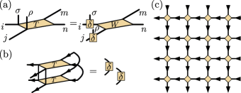
Figure 1: Construction of isoTNS: Each yellow node labels a tensor. (a) Each tensor has two physical legs ($\sigma$ and $\rho$) and four virtual legs $i,j,m,n$. The local tensor $T$ is a product of some matrix $W$ and two $\delta$-tensors. The $\delta$-tensor is 1 when all the legs are equal, and zero otherwise. (b) The isometry condition. The contraction of the tensor $T$ with its complex conjugate (depicted with flipped physical legs) yields two two-leg $\delta$-tensors. The arrows indicate the direction of the contraction. (c) The wavefunction is obtained by contracting the virtual legs of the tensors. The physical legs of the tensors, which encode the physical spins, are omitted.

The search for exotic quantum phases of matter is a central theme in condensed matter physics. While the last decades have witnessed tremendous progress in our theoretical understanding of topologically ordered phases, physical realization of topological phases remains a significant challenge, with the fractional quantum Hall effect [1] representing one of the few unambiguous examples in the solid state. The advent of programmable quantum hardware has opened up unprecedented avenues for accessing novel quantum states. Recently, breakthroughs were made in the realization of topologically ordered states using Rydberg simulators [2, 3], superconducting qubits [4, 5] and trapped ions [6, 7]. While these realizations focused on specific topological states, the important question of realizing the topological quantum phase transitions is more challenging. Progress has been made in one-dimensional (1D) systems by exploiting the correspondence between sequential quantum circuits and matrix-product states (MPS) [8]. The exact ground states across certain quantum phase transitions can be represented by a parameterized MPS with a finite bond dimension and can be physically realized using its efficient quantum circuit representation [9, 10, 11]. While general two-dimensional (2D) tensor-network states (TNS) with a finite bond dimension can describe exact ground states across various quantum phase transitions—including some critical states with a power-law correlation [12, 13, 14, 15, 16, 17, 18, 19], the convenient correspondence between sequential quantum circuits and TNS similarly to 1D is lacking in 2D. Recently, measurements are explored as a tool for generating such 2D TNS-solvable ground states [20, 21]. However, post-selection among exponentially many outcomes is required.

To address this question, we investigate quantum phase transitions between states exactly representable by 2D isometric tensor-network states (isoTNS) [22]. IsoTNS form a subclass of 2D TNS with an additional isometry condition and can represent a large class of gapped quantum phases [23]. The isometry condition inherent in isoTNS establishes a 2D analogue of the canonical form in 1D MPS and directly leads to the correspondence between isoTNS and linear sequentially generated quantum circuits [22, 24]. We can therefore construct efficient quantum circuits for realizing quantum phase transitions by identifying isoTNS of interest.

In this work, we propose a simple “plumbing” method to construct exact isoTNS such that the coefficients in the wavefunction can be associated with the Boltzmann weights of certain 2D classical partition functions. By introducing an internal parameter, the system can be deformed continuously from one phase to another phase via a quantum phase transition. We illustrate this method by constructing a quantum phase transition in the ground states between symmetry-enriched topological (SET) phases, where the system has an intrinsic $\mathbb{Z}_{2}$ topological order enriched by an anti-unitary $\mathbb{Z}_{2}^{T}$ symmetry. We discuss the properties of the ground state both away from and at the transition point.

Isometric Tensor Networks and Classical Partition Functions. We focus our discussion on the 2D systems, the generalization of the construction to arbitrary higher dimensions is straightforward. We begin by briefly reviewing the concept of 2D TNS. Consider a 2D spin system on a square lattice with local Hilbert space dimension $d$ and each spin is located on the edges of the square lattice. A 2D TNS can be defined via a rank-6 local tensor $T^{\sigma\rho}_{ijmn}$ at each vertex, where $\sigma$ ($\rho$) represents the spin degree of freedom on the left (bottom) edge connected to the vertex. The legs $i,j,m,n$ label the virtual degrees of freedom (Fig. 1a). The dimension of the virtual legs is referred to as bond dimension. For a translationally invariant system with $N$ spins, the wavefunction is obtained by contracting the neighbouring virtual legs of all the tensors

$$\ket{\psi}=\sum_{\sigma_{1},\cdots,\sigma_{N}}\text{tTr}\left(\{T^{\sigma_{1}\sigma_{2}},\cdots,T^{\sigma_{N-1}\sigma_{N}}\}\right)\ket{\sigma_{1},\cdots,\sigma_{N}},$$ (1)

where tTr denotes the tensor contraction.

Classical partition functions can be encoded in the TNS with a finite bond dimension [12], such that the squared norm of the coefficients in the wavefunction is equal to the Boltzmann weights in the classical partition function [25]. The thermal phase transition in the classical system is mapped to a quantum phase transition, where the classical criticality is mapped to criticality in the wavefunction. We consider the restriction of this class of tensor networks to isoTNS. To achieve this, we impose the following conditions on the local tensors: (i) The local tensor $T^{\sigma\rho}_{ijmn}$ can be decomposed as

$$T^{\sigma\rho}_{ijmn}=\sum_{i^{\prime},j^{\prime}}\delta^{\sigma}_{ii^{\prime}}\delta^{\rho}_{jj^{\prime}}W_{i^{\prime}j^{\prime}mn},$$ (2)

where $W_{i^{\prime}j^{\prime}mn}$ is a $d^{2}\times d^{2}$ matrix and $\delta^{\sigma}_{ab}$ denotes a “plumbing” $\delta$-tensor such that $\delta^{\sigma}_{ab}=1$ if $\sigma=a=b$, and zero otherwise. This relation is depicted in Fig. 1a. This condition relates the quantum wavefunction to a classical partition function in the following way: The tensor $\delta^{\sigma}_{ab}$ makes the virtual legs equivalent to the physical degrees of freedom in the quantum system. As a result, the probabilities for the spin configurations at each vertex in the tensor-network wavefunction are encoded in a local tensor $R_{ijmn}=|W_{ijmn}|^{2}$, where $R$ is a weight matrix for spin states $i,j,m,n$ around the vertex. The transfer matrix of the isoTNS is thus the same as the transfer matrix for a classical partition function contracted from the local weight matrix (see the Supplemental Material (SM) [26]). (ii) We enforce an isometry condition on the local tensor $T^{\sigma\rho}_{ijmn}$. More precisely, we require

$$\sum_{\sigma,\rho,m,n}\left(T^{\sigma\rho}_{ijmn}\right)^{*}T^{\sigma\rho}_{i^{\prime}j^{\prime}mn}=\delta_{ii^{\prime}}\delta_{jj^{\prime}}.$$ (3)

This is pictorially shown in Fig. 1b. The set of TNS satisfying this condition is isoTNS. For the plumbed isoTNS satisfying Eq (2), the 2D isometry condition Eq. (3) is satisfied if and only if

$$\sum_{m,n}|W_{ijmn}|^{2}=1,\ \forall i,j.$$ (4)

For a given bond dimension, the $W$-matrix representing the plumbed isoTNS forms a finite dimensional manifold. Our strategy is to search for continuous paths within this manifold that connect between ground states having different quantum phases. It is worth mentioning that in 1D the plumbed isoTNS is a subclass of the canonical form for 1D matrix-product states (MPS). Simple examples of quantum phase transitions previously known in MPS [9] can also be constructed using the plumbing construction (see the SM [26]).

A Continuous IsoTNS Path Between Symmetry-Enriched Topological Phases Crossing a Quantum Critical Point. Let us consider a spin-1/2 system where each spin is encoded by a qubit with the Pauli basis such that $Z\ket{0}=\ket{0}$ and $Z\ket{1}=-\ket{1}$. The physical leg of the tensor has dimension $d=2$, Eq. (2) implies that the plumbed isoTNS has bond dimension $D=d=2$. The toric code ground state with $\mathbb{Z}_{2}$ topological order [27] naturally falls into this family of isoTNS, with

$$W^{(\text{TC})}=\pNiceMatrix[first-row,last-col]\ket{00}&\ket{01}\ket{10}\ket{11}\\ \frac{1}{\sqrt{2}}00\frac{1}{\sqrt{2}}\ \ket{00}\\ 0\frac{1}{\sqrt{2}}\frac{1}{\sqrt{2}}0\ \ket{01}\\ 0\frac{1}{\sqrt{2}}\frac{1}{\sqrt{2}}0\ \ket{10}\\ \frac{1}{\sqrt{2}}00\frac{1}{\sqrt{2}}\ \ket{11}\\ ,$$ (5)

where the indices label the legs $i.j,m,n$ in $W_{ijmn}$. If we view $\ket{1}$ as occupied by a string and $\ket{0}$ as empty, the eight non-zero entries in $W$ are exactly the eight vertex configurations with no broken strings. The resulting wavefunction is an equal-weight superposition of all the closed-loop configuration as we expect from the toric code ground state. Consider the following continuous path of $W$-matrix for $g\in[-1,1]$

$$W(g)=\left(\begin{matrix}\frac{1}{\sqrt{1+|g|}}&0&0&\text{sign}(g)\sqrt{\frac{|g|}{1+|g|}}\\ 0&\frac{1}{\sqrt{2}}&\frac{1}{\sqrt{2}}&0\\ 0&\frac{1}{\sqrt{2}}&\frac{1}{\sqrt{2}}&0\\ \sqrt{\frac{|g|}{1+|g|}}&0&0&\frac{1}{\sqrt{1+|g|}}\end{matrix}\right),$$ (6)

where the function sign$(g)$ picks up the sign of $g$. At $g=1$, we recover the exact toric code. At $g=-1$, the $W$-matrix differs from the toric code $W^{(\text{TC})}$ by a minus sign for one of the vertex configurations. This implies that the wavefunction is related to the toric code ground state by a finite-depth local quantum circuit. However, as we will show below that, the two limits belong to distinct quantum phases due to the presence of physical symmetries.

The ground state along this path respects an anti-unitary $\mathbb{Z}_{2}^{T}$ symmetry generated by the global spin flip composed with complex conjugation $\left(\prod_{i}X_{i}\right)K$. While at $g=1$, the system is the usual toric code with only an intrinsic $\mathbb{Z}_{2}$ topological order, at $g=-1$ the TNS describes a ground state with a non-trivial symmetry-enriched topological (SET) order, where the $\mathbb{Z}_{2}$ topological order is enriched by $\mathbb{Z}_{2}^{T}$ symmetry. Along the path, there exists a $\mathbb{Z}_{2}^{T}$-symmetric local parent Hamiltonian which remains frustration-free and continuous in $g$ (see the SM [26]).

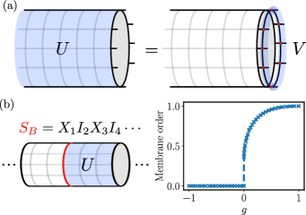
Figure 2: Detecting SET order: (a) Physical symmetry $U$, consisting of Pauli $X$ on all the qubits in the bulk, is mapped to a virtual matrix-product operator (MPO) $V$ on the boundary formed by the uncontracted virtual legs of the tensors. (b) The membrane order $\mathcal{M}$ computed on the minimally entangled ground state corresponding to the anyon e at the thermodynamic limit. The numerical method for extracting the membrane order is described in Ref. [19]. Here $S_{B}$ is the appropriated string operator inserted at the boundary of the partial action of the physical symmetry.

Recall that a topologically ordered system has a non-trivial SET order when the anyonic excitations of the system transform non-trivially under the physical symmetries [28, 29, 30, 31]. The SET order in the ground state can be diagnosed by inspecting how the action of the physical symmetries on the bulk relates to a non-trivial action on the open boundary of the system; the boundary action carries labels that characterize the phases of the system [32, 33, 34]. To see this explicitly, we consider a cylindrical geometry with open ends. At the boundary, the uncontracted virtual bonds of the TNS form an effective 1D system (see Fig. 2a). Suppose a physical symmetry $U$ is applied to the ground state in the bulk; this physical action is equivalent to a virtual action of a boundary operator $V$. Using the TNS defined by Eq. (6) on a cylinder with circumference $L\in 4\mathbb{N}$, we have

$$U=\prod_{i}X_{i}\to V(g)=\left(\prod_{b}X_{b}\right)\text{sign}(g)^{\frac{n(n-1)}{2}},$$ (7)

where $b$ labels the virtual bonds forming the effective boundary spin-1/2 system and $n=\sum_{b}(1-Z_{b})/2$ is a sum of Pauli $Z$ matrices at each virtual bond ($n$ essentially counts the number of states $\ket{1}$ on the boundary). For $\mathbb{Z}_{2}^{T}$ symmetry, a discrete label for the SET phase can be obtained from $V(g)^{*}V(g)=\text{sign}(g)^{P}$, where $*$ denotes the complex conjugation and $P$ is the parity of the boundary spin system. Different parity $P$ corresponds to distinct anyon labels carried by the minimally entangled states [35]. In our convention, $P=0$ labels the trivial quasiparticle while $P=1$ labels the vertex excitation (i.e. the e anyon) in the toric code. For a given parity, the quantity $V(g)^{*}V(g)$ is a discrete invariant that labels the elements in the second cohomology group $H^{(2)}(\mathbb{Z}_{2}^{T},\mathbb{Z}_{2})=\mathbb{Z}_{2}$, which classifies the symmetry fractionlization patterns on the anyons in $\mathbb{Z}_{2}$ topological order under $\mathbb{Z}_{2}^{T}$ symmetry (without permutation of anyons) [28, 36]. Therefore, the symmetry fractionlization patterns on the e anyon are distinct for $g>0$ and $g<0$, the system belongs to different SET phases, with the phase transition occurring at $g=0$.

Distinct SET orders cannot be measured via any local order parameters, but they can be distinguished via a non-local membrane order parameter [37, 38], which generalizes the usual string order parameters for 1D symmetry-protected topological (SPT) phases [39, 40]. Consider the system on an infinite cylinder and let $L$ be the circumference, a suitable membrane order parameter in this case is given by $\mathcal{M}=\lim_{L\to\infty}|\bra{\psi}S_{B}U_{\text{subsys}}S_{B}\ket{\psi}|^{1/L}$, where $U_{\text{subsys}}=\prod_{i\in\text{subsys}}X_{i}$ is the symmetry $U$ acting only partially on the bulk and the closed string operator $S_{B}=X_{1}I_{2}X_{3}I_{4}\cdots X_{L-1}I_{L}$ around the cylinder is the operator on the boundary of $U_{\text{subsys}}$. In Fig. 2b, we show the membrane order for the minimally entangled state labeling the e anyon. At $g<0$, a non-trivial symmetry fractionlization over the anyon leads to $\mathcal{M}=0$ due to a superselection rule [41], while $\mathcal{M}\neq 0$ for $g>0$ corroborates the absence of non-trivial symmetry fractionlization.

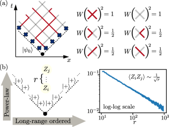
Figure 3: Quantum critical point at $g=0$: (a) The system in Fig. 1c is rotated 45 degrees anticlockwise. The isoTNS is contracted from some boundary state $\ket{\psi_{0}}$ formed by the boundary qubits (dark blue crosses). An example configuration in the wavefunction is shown. The red line denotes $\ket{1}$ and the grey line denotes $\ket{0}$. The particles are located at the endpoints of the red lines and emanate from the boundary (dashed line). They move according to stochastic jumps determined by the $W$-matrix. (b) The correlation along the $t$-direction averaging over $2\times 10^{6}$ classical trajectories. Here $\ket{+}=(\ket{0}+\ket{1})/\sqrt{2}$. The correlator shows a power law decay with an exponent $1/2$.

Power-Law Correlation at the Quantum Critical Point and Dynamics of 1D Classical Systems. Along the entire isoTNS path, the classical weight matrix associated with the isoTNS from Eq. (6) is the same as the weight matrix of the classical eight-vertex model which is exactly solvable [42]. At the SET transition point $g=0$, the classical eight-vertex model reduces to a gapless point of the six-vertex model. Interestingly, the corresponding transfer matrix of the six-vertex model has the same spectrum as the Hamiltonian of the 1D ferromagnetic Heisenberg XXX chain (they are solved by the same Bethe Ansatz [42]), exhibiting a spectral gap closing of $O(1/L^{2})$. The Heisenberg chain has a long-range order in space and it can support power-law temporal correlation. By analogy, we expect the 2D critical wavefunction to exhibit a similar anisotropy in the correlation functions along the two spatial directions.

In the gapped phases (i.e. $g\neq 0$), the boundary conditions are irrelevant for the bulk properties. However, they become important at the transition point $g=0$. It is convenient to rotate the lattice in Fig. 1c anticlockwise by 45 degrees and consider the system on a planar geometry with open boundaries. The isoTNS is then obtained by initializing the tensor network contraction from an arbitrary 1D boundary state $\ket{\psi_{0}}$ formed by the qubits at the bottom boundary (see Fig. 3a). The resulting critical wavefunction respects a conservation law: The number of lines formed by states $\ket{1}$ is conserved across any horizontal slice, unless they terminate on the boundary. A snapshot of the wavefunction is given in Fig. 3a. This conservation law reveals a direct relation between the quantum critical ground state and the dynamics of an 1D classical system. Suppose the boundary state $\ket{\psi_{0}}$ is a product state in the Pauli-$Z$ basis and we interpret the endpoint vertex of a string of state $\ket{1}$ as being occupied by a particle. In this picture, the conservation law is simply that of the particle number. As the tensor network is sequentially contracted from the bottom to the top, the particles are moving forward in time and tracing out their worldlines (the $x$- and $t$-direction in Fig. 3a). The Floquet-type dynamics are generated by stochastic jumps with probability given by the matrix elements $|W_{ijmn}|^{2}$. At a given time $t$, a single particle either moves to the left or to the right along the $x$-direction with an equal probability. If two particles meet at the same vertex, they bounce away from each other. The classical picture suggests that the critical wavefunction is a superposition of all the worldlines of the particles emanating from the boundary.

A few properties of the critical wavefunction follow directly from the classical picture. (i) The critical wavefunction can have a long-range order along the $x$-direction. This long-range order comes from the long-range order at the boundary state $\ket{\psi_{0}}$ due to the particle-number conservation: The number of states $\ket{1}$ at any row along the $x$-direction is determined by the number of states $\ket{1}$ in $\ket{\psi_{0}}$. (ii) The critical wavefunction can support correlation with a power-law decay along the $t$-direction. To see this, suppose the boundary state $\ket{\psi_{0}}$ only contains few particles. The moving particles have a small chance of interacting with each other and the process thus behaves similarly to an independent random walk with diffusive dynamics. More generally, the process is an example of the nonunitary Floquet XXX model [43, 44, 45]. We verify the power-law correlation by computing the spin-spin correlation $\langle Z_{i}Z_{j}\rangle$ between sites $i,j$ in the bulk along the $t$-direction for the boundary condition $\ket{\psi_{0}}=\ket{++\cdots+}$, where $\ket{+}=(\ket{0}+\ket{1})\sqrt{2}$. This boundary condition is an equal-weight superposition of all the possible classical initial conditions. The resulting correlation corresponds to the typical correlation function over this ensemble. The result is shown in Fig. 3b, a clear power-law decay as $1/\sqrt{r}$ can be seen, which is consistent with a diffusive behaviour. In the SM [26], we show that the correlation along a direction between the $t$- and the $x$-direction falls off exponentially.

Figure 4: Quantum circuit: (a) A parametrized 4-qubit gate generating the isoTNS. The gate is decomposed into a single-qubt gate, two-qubit CNOT gates and a control-rotation gate. An additional three-qubit gate is included for $g<0$. Here, $A(g)$ and $B(g)$ are single-qubit gates such that $A(g)\ket{0}=\sqrt{1/(1+|g|)}\ket{0}+\sqrt{|g|/(1+|g|)}\ket{1}$ and $B(g)=A(g)^{{\dagger}}H$, where $H$ is the Hadamard gate. The three-qubit gate is a CCZ gate such that $\text{CCZ}\ket{111}=-\ket{111}$ and it acts trivially otherwise. (b) Initialization. The physical qubits (blue crosses) are located at the edges of a square lattice. The system is initialized as $\ket{\psi_{0}}\otimes\ket{00\cdots 0}$, where $\ket{\psi_{0}}$ is the boundary state. (c) Generating the isoTNS. The gate in (a) is applied diagonally in parallel. The red shade marks the spread of the entanglement.

Quantum Circuit Representation. The quantum circuit representation for the isoTNS path can be easily found when the system is defined with open boundaries. The isoTNS tensor is mapped to a 4-qubit quantum gate acting on each vertex, as shown in Fig. 4a. The system is initialized as $\ket{\psi_{0}}\otimes\ket{00\cdots 0}$, where $\ket{\psi_{0}}$ is any 1D quantum state formed by the boundary qubits (see Fig. 4b). The state is generated by sequentially applying the 4-qubit gate to each vertex along the diagonal direction, as depicted in Fig. 4c. The depth of the circuit thus scales as $O(L)$ as long as the boundary state $\ket{\psi_{0}}$ can be prepared with an $O(L)$-depth circuit. Using the exact quantum circuit, the ground states along the entire path can be realized without any post-selection.

Discussion and outlook. Here, we have focused on the isoTNS path interpolating between distinct SET phases. The same construction can be applied to find isoTNS paths between other topological phases. For example, the tensor-network solvable path, which is previously noted in Ref. [46], is in fact an isoTNS path that can be constructed with the plumbing method. This path interpolates between two 1-form SPT phases with the exact toric code ground state being the critical wavefunction. Another interesting example is to consider a path between two intrinsically topological phases. By adapting the plumbing method to the domain walls of tensor-network virtual legs (the double-line TNS [47]), we expect that an isoTNS path with bond dimension $D=4$ can be constructed between the toric code and the double-semion ground state with distinct $\mathbb{Z}_{2}$ topological order [48, 49], crossing the same critical point as the SET case. The isoTNS path will be analogous to the $D=4$ non-isometric TNS path studied in Ref. [13], which crosses a critical point with a different six-vertex criticality. An exciting direction is to explore the possibility of connecting generic gapped quantum phases via continuous isoTNS paths.

It has been known that the typical correlation in isoTNS follows an exponential decay [50]. An open question remained whether isoTNS can support power-law correlation. In our work, by giving a concrete example, we show that this is indeed possible. More intriguingly, we find that the power-law decay in the example originates from a direct connection between the worldlines of 1D stochastic dynamics and 2D isoTNS ground states. Whether this connection leads to more interesting isoTNS is an open question. The efficient physical realization of 2D topological quantum phase transitions is also valuable resource for performing and benchmarking algorithms for quantum phase recognition in higher than 1D [51, 52].

Acknowledgement We thank Robijn Vanhove, Wen-Tao Xu, Xie-Hang Yu and Tomaž Prosen for inspiring discussions. Y.-J.L. and F.P. acknowledge support from the Deutsche Forschungsgemeinschaft (DFG, German Research Foundation) under Germany’s Excellence Strategy–EXC–2111–390814868 and innovation programme (Grant Agreement No. 851161), as well as the Munich Quantum Valley, which is supported by the Bavarian state government with funds from the Hightech Agenda Bayern Plus.

Data and materials availability: Data analysis and simulation codes are available on Zenodo upon reasonable request [53].

Appendix A The plumbing construction in 1D MPS

The plumbing method can be applied to the 1D system and we recover some of the familiar examples of quantum phase transitions in 1D matrix-product states (MPS) [9]. MPS are an ansatz class where the coefficients of a full 1D $N$-qubit state $\ket{\psi}$ are decomposed into products of matrices. Explicitly, for a system with open boundaries and translational invariance in the bulk

$$\begin{split}\ket{\psi}=\sum\limits_{\{\sigma\}}&A^{\sigma_{1}}B^{\sigma_{2}}B^{\sigma_{3}}\dots B^{\sigma_{n-1}}C^{\sigma_{n}}\ket{\sigma_{1}\sigma_{2}\sigma_{3}\dots\sigma_{n}},\end{split}$$ (8)

where the $\sigma_{k}\in\{0,1,\cdots,d\}$ indices are the physical indices and $B^{\sigma}$ are $\chi\times\chi$ matrices with $\chi$ being the bond dimension of the MPS. The boundary tensors $A^{\sigma}$ and $C^{\sigma}$ are $1\times\chi$ and $\chi\times 1$ matrices, respectively. Analogous to the main text, we employ the plumbing structure and impose the isometry condition. Namely, we require

$$B^{\sigma}_{ij}=\sum_{j^{\prime}}\delta^{\sigma}_{ij^{\prime}}W_{j^{\prime}j},$$ (9)

where the $\delta$-tensor takes value 1 when all indices are the same and zero otherwise. Furthermore

$$\sum_{\sigma,j^{\prime}}\left(B^{\sigma}_{ij^{\prime}}\right)^{*}B^{\sigma}_{jj^{\prime}}=\delta_{ij}.$$ (10)

This isometry condition is satisfied if and only if

$$\sum_{j}|W_{ij}|^{2}=1,\ \forall i.$$ (11)

Now suppose we take $C^{\sigma}_{i}=\delta^{\sigma}_{i}$ and $A^{\sigma}$ is some boundary condition that can be chosen at will. The MPS in Eq. (8) is essentially a canonical form of the MPS [54], which is equivalent to a sequential quantum circuit [8].

As an example, consider a $W$-matrix path with $d=\chi=2$, for $g\in[-1,1]$

$$W(g)=\pNiceMatrix[first-row,last-col]\ket{0}&\ket{1}\\ \frac{1}{\sqrt{1+|g|}}\text{sign}(g)\sqrt{\frac{|g|}{1+|g|}}\ \ket{0}\\ \sqrt{\frac{|g|}{1+|g|}}\frac{1}{\sqrt{1+|g|}}\ \ket{1}.$$ (12)

At $g=1$, the wavefunction $\ket{\psi(g)}$ is a simple product state $\ket{++\cdots+}$ in the bulk. At $g=-1$, the state is a cluster state with $Z_{i}X_{i+1}Z_{i+2}\ket{\psi(-1)}=-1$ for all $i$ in the bulk. At these two limits, the 1D system belongs to distinct 1D SPT phases protected by anti-unitary $\mathbb{Z}_{2}^{T}$ symmetry generated by $\left(\prod_{i}X_{i}\right)K$, where $K$ is the complex conjugation. It can be verified that this is a symmetry for the state for all $g$.

A quantum phase transition happens at $g=0$, where the wavefunction has a long-range order and becomes the Greenberger–Horne–Zeilinger (GHZ) state $\ket{\psi(0)}=(\ket{00\cdots 0}+\ket{11\cdots 1})/\sqrt{2}$ with the boundary tensor chosen as $A^{\sigma}_{i}=\delta^{\sigma}_{i}$. In fact, the MPS along this path is exactly the canonical form of the $\chi=2$ MPS considered in Ref. [9], with a parent Hamiltonian

$$H(g)=g_{zxz}\sum_{i}Z_{i-1}X_{i}Z_{i+1}-g_{zz}\sum_{i}Z_{i}Z_{i+1}-g_{x}\sum_{i}X_{i},$$ (13)

where $g_{zxz}=(1-g)^{2},g_{x}=(1+g)^{2}$ and $g_{zz}=2(1-g^{2})$. This canonical form has been utilized to construct an efficient quantum circuit for the physical realization of this phase transition on a digital quantum computer [11].

Appendix B Anisotropic correlation at the quantum critical point

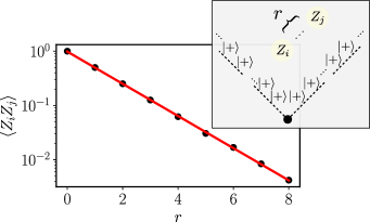
Figure 5: The two-point correlation along the 45-degree direction exhibits an exponential decay. The plot is displayed with log scale in the $y$-axis. The black dots are the results from Monte Carlo sampling over $1.5\times 10^{6}$ samples on a system of $21\times 21$ plaquettes. The red line is a linear fit with a gradient around -0.68.

In the main text, we show that at the critical point with a boundary state $\ket{\psi_{0}}=\ket{++\cdots+}$, the two-point correlation along a particular spatial dimension decays algebraically. Along other spatial directions, we expect that the correlation decays exponentially, similarly to the spatial-temporal correlation for a single random walker in the 1D classical dynamics.

We note that along the $x$-direction in Fig. 3a, the spin-spin correlation $\langle Z_{i}Z_{j}\rangle$ vanishes due to the disordered boundary state. To further verify the correlation, suppose now we measure the correlation along the 45-degree angle (see Fig. 5), a clear exponential decay is observed. More generally, when $\langle Z_{i}Z_{j}\rangle$ is measured along a direction different from the $t$-direction in Fig.3a, we expect that the correlation decays exponentially with an angle-dependent correlation length.

Appendix C Quantum-classical correspondence

In this section, we describe the connection between the plumbing construction and the quantum-classical correspondence in tensor networks. We note that the squared norm of the TNS wavefunction represented by the plumbed local tensor $T^{\sigma\rho}_{ijmn}$ can be expressed as the product of the transfer operators $\langle\psi|\psi\rangle=\Tr(M^{L})$ (assuming periodic boundary condition on an $L\times L$ system). The transfer operator $M=R_{1}R_{2}\cdots R_{L}$ is the product of the weight matrix $R$ along each row, where $R_{ijmn}=|W_{ijmn}|^{2}$ and $W$ is the $W$-matrix used in the plumbing procedure. One way to contract the transfer operator can be visualized as

$$\includegraphics[scale={1}]{sm_tns.pdf}.$$ (14)

Indeed, one can also rotate each weight matrix $R$ by 45 degress and contract. This is exactly the same as contracting a 2D classical partition function. As an example, consider an $L\times L$ classical spin system on a square lattice with nearest-neighbour two-body interaction $H=\sum_{\langle i,j\rangle}h(\sigma_{i},\sigma_{j})$. The partition function of the system $\mathcal{Z}=\Tr(e^{-\beta H})=\Tr(M^{L})$ can be conveniently expressed using the transfer matrix $M=R_{1}R_{2}\cdots R_{L}$, where $(R_{k})_{ijmn}=\sum_{\sigma}\exp\left[-\beta\left(h(i,\sigma)+h(j,\sigma)+h(\sigma,m)+h(\sigma,n)\right)\right]$ is the local weight matrix that carries the statistical weights associated with the coupling between the $k$-the spin along each row and its neighbours. The 2D classical model can thus be mapped to a 2D quantum model using the plumbing construction.

Appendix D A parent Hamiltonian for the isoTNS path between SET phases

In this section, we derive the parent Hamiltonian for the isoTNS path presented in the main text. Let us consider the toric code described by the Hamiltonian defined on the same square lattice as in the main text,

$$H_{\text{TC}}=\sum_{v}\mathcal{A}_{v}+\sum_{p}\mathcal{B}_{p},$$ (15)

where $\mathcal{A}_{v}=(1-\prod_{i\in v}Z_{i})/2$ and $\mathcal{B}_{p}=(1-\prod_{i\in p}X_{i})/2$ are projectors made from products of Pauli operators around each vertex $v$ and each plaquette $p$. The vertex and the plaquette operators commute with each other and the ground state $\ket{\text{TC}}$ satisfies $\mathcal{A}_{v}\ket{\text{TC}}=\mathcal{B}_{p}\ket{\text{TC}}=0$ for all $v,p$. For $g>0$, the isoTNS path between the SET phases can be obtained from the toric code ground state by an imaginary time evolution

$$\ket{\Psi(g)}=\mathcal{T}(\beta_{1},\beta_{2})\ket{\text{TC}}=\prod_{v}e^{\beta_{1}P^{(1)}_{v}+\beta_{2}P^{(2)}_{v}}\ket{\text{TC}},$$ (16)

where the projectors at each vertex $v$ are defined as

$$P^{(1)}_{v} =\frac{1}{6}(1+Z_{v(A)}Z_{v(B)})(1+Z_{v(C)}Z_{v(D)})(1+Z_{v(A)}Z_{v(D)}),$$ (17)

$$P^{(2)}_{v} =\frac{1}{6}(1+Z_{v(A)}Z_{v(B)})(1+Z_{v(C)}Z_{v(D)})(1-Z_{v(A)}Z_{v(D)}).$$ (18)

Note that here we use the labeing convention

$$\includegraphics[scale={1}]{sm_v.pdf}.$$ (19)

The parameters are related to $g$ via

$$\beta_{1} =\frac{1}{2}\left(\log 2-\frac{1}{2}\log(1+|g|)\right),$$ (20)

$$\beta_{2} =\frac{1}{2}\left(\log 2-\frac{1}{2}\log(1+|g|)\right)+\frac{1}{2}\log g.$$ (21)

To derive a local parent Hamiltonian, we employ the method in Ref. [19]. Since $(b_{p}\mathcal{T}b_{p}\mathcal{T}^{-1}-b_{p})\ket{\Psi(g)}=0$, where $b_{p}=\prod_{i\in p}X_{i}$. If follows that

$$\left(e^{\Lambda_{a}+\Lambda_{c}+O_{b}+O_{d}}-b_{p}\right)\ket{\Psi(g)}=0,$$ (22)

where we use the following labeling convention for the vertices on each plaquette

$$\includegraphics[scale={1}]{sm_plaq.pdf}.$$ (23)

The operators at each vertex are defined as

$$\Lambda_{v} =-\frac{1}{3}(\beta_{1}-\beta_{2})\left(1+Z_{v(A)}Z_{v(B)}\right)\left(1+Z_{v(C)}Z_{v(D)}\right)Z_{v(A)}Z_{v(D)},$$

$$O_{v} =-\frac{1}{3}\left(Z_{v(A)}Z_{v(B)}+Z_{v(C)}Z_{v(D)}\right)\left[(\beta_{1}+\beta_{2})+(\beta_{1}-\beta_{2})Z_{v(A)}Z_{v(D)}\right].$$ (24)

We can use this observation to obtain a suitable local term in the parent Hamiltonian. It is possible to choose a path slightly deviated from, but continuously connected to Eq. (20) such that the resulting wavefunction Eq. (16) is analytic in $g$ for $g\in(-1,1)$. The definition of the parameters $\beta_{1},\beta_{2}$ can then be extended to $g<0$ using an argument in Ref. [19] based on analytic continuation. The path Eq. (20) is therefore also valid for $g\in[-1,1]$, where we define $\log g=\log|g|+i\pi$ for $g<0$. As a sanity check, it can be verified that the wavefunction Eq. (16) at $g=-1$ is the same as the SET isoTNS wavefunction discussed in the main text (up to an overall phase factor). Therefore, all the analysis for $g>0$ can be straightforwardly extended to the case $g<0$.

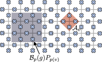
Figure 6: A local parent Hamiltonian for the isoTNS ground states in the main text. The Hamiltonian is frustration-free and consists of projectors around each plaquette (the shaded 10 qubits) and each vertex (shaded 4 qubits).

Figure 7: Energy spectrum from the exact diagonalization of a system with $4\times 2$ plaquettes (16 qubits) and periodic boundary condition. The plot shows the low-lying eigenvalues of the Hamiltonian. At $g=\pm 1$, the models are fixed points of the topological phases with an energy gap $\Delta=2$.

To proceed, note that

$$\left(e^{\Lambda_{a}+\Lambda_{c}+O_{b}+O_{d}}-b_{p}\right)^{2}=$$

$$\quad 2\cosh(\Lambda_{a}+\Lambda_{c}+O_{b}+O_{d})\left(e^{\Lambda_{a}+\Lambda_{c}+O_{b}+O_{d}}-b_{p}\right).$$ (25)

We can therefore define a new plaquette projector as

$$\mathcal{B}_{p}(g)P_{p(v)}=$$

$$\quad\frac{\sech(\Lambda_{a}+\Lambda_{c}+O_{b}+O_{d})}{2}\left(e^{\Lambda_{a}+\Lambda_{c}+O_{b}+O_{d}}-b_{p}\right)P_{p(v)}.$$ (26)

where $P_{p(v)}$ is the projector onto the closed loop configuration around each plaquette $p$, i.e. $P_{p(v)}=\prod_{v\in p}(1-\mathcal{A}_{v})$. It is included to ensure that $\mathcal{B}_{p}(g)P_{p(v)}$ remains Hermitian and therefore a projector for $g\in[-1,1]$. The operator hypobolic secant function is defined as $\sech(O)\equiv 1/\cosh(O)$ within the subspace $P_{p(v)}=1$, and $\sech(O)\equiv 0$ in the subspace $P_{p(v)}=0$. A local frustration-free parent Hamiltonian is thus given by

$$H(g)=\sum_{v}\mathcal{A}_{V}+\sum_{p}\mathcal{B}_{p}(g)P_{p(v)},$$ (27)

with a ground-state energy of zero. The support of each term in $H(g)$ is depicted in Fig. 6. When the system is defined on a torus (periodic boundary condition), $H(g)$ is gapped and the ground states are exactly four-fold degenerate for $g\neq 0$. At $g=0$, the system is gapless. In addition, the $\mathbb{Z}_{2}^{T}$ symmetry is satisfied, i.e. $[H(g),\left(\prod_{i}X_{i}\right)K]=0$ for $g\in[-1,1]$. The low-lying spectrum of the Hamiltonian on a square lattice with $4\times 2$ plaquettes (16 qubits) is shown in Fig. 7. Note that the parent Hamiltonian for the ground states is not unique, the one derived here is one of the possible parent Hamiltonians.

References

- Tsui et al. [1982] D. C. Tsui, H. L. Stormer, and A. C. Gossard, Two-dimensional magnetotransport in the extreme quantum limit, Phys. Rev. Lett. 48, 1559 (1982).
- Semeghini et al. [2021] G. Semeghini, H. Levine, A. Keesling, S. Ebadi, T. T. Wang, D. Bluvstein, R. Verresen, H. Pichler, M. Kalinowski, R. Samajdar, A. Omran, S. Sachdev, A. Vishwanath, M. Greiner, V. Vuletić, and M. D. Lukin, Probing topological spin liquids on a programmable quantum simulator, Science 374, 1242 (2021).
- Verresen et al. [2021] R. Verresen, M. D. Lukin, and A. Vishwanath, Prediction of toric code topological order from Rydberg blockade, Phys. Rev. X 11, 031005 (2021).
- Satzinger et al. [2021] K. J. Satzinger, Y.-J. Liu, A. Smith, C. Knapp, M. Newman, C. Jones, Z. Chen, C. Quintana, X. Mi, A. Dunsworth, et al., Realizing topologically ordered states on a quantum processor, Science 374, 1237 (2021).
- Liu et al. [2022] Y.-J. Liu, K. Shtengel, A. Smith, and F. Pollmann, Methods for simulating string-net states and anyons on a digital quantum computer, PRX Quantum 3, 040315 (2022).
- Iqbal et al. [2023] M. Iqbal, N. Tantivasadakarn, R. Verresen, S. L. Campbell, J. M. Dreiling, C. Figgatt, J. P. Gaebler, J. Johansen, M. Mills, S. A. Moses, J. M. Pino, A. Ransford, M. Rowe, P. Siegfried, R. P. Stutz, M. Foss-Feig, A. Vishwanath, and H. Dreyer, Creation of non-abelian topological order and anyons on a trapped-ion processor (2023), arXiv:2305.03766 [quant-ph] .
- Tantivasadakarn et al. [2023a] N. Tantivasadakarn, R. Verresen, and A. Vishwanath, Shortest route to non-abelian topological order on a quantum processor, Phys. Rev. Lett. 131, 060405 (2023a).
- Schön et al. [2005] C. Schön, E. Solano, F. Verstraete, J. I. Cirac, and M. M. Wolf, Sequential generation of entangled multiqubit states, Phys. Rev. Lett. 95, 110503 (2005).
- Wolf et al. [2006] M. M. Wolf, G. Ortiz, F. Verstraete, and J. I. Cirac, Quantum phase transitions in matrix product systems, Phys. Rev. Lett. 97, 110403 (2006).
- Jones et al. [2021] N. G. Jones, J. Bibo, B. Jobst, F. Pollmann, A. Smith, and R. Verresen, Skeleton of matrix-product-state-solvable models connecting topological phases of matter, Phys. Rev. Res. 3, 033265 (2021).
- Smith et al. [2022] A. Smith, B. Jobst, A. G. Green, and F. Pollmann, Crossing a topological phase transition with a quantum computer, Phys. Rev. Research 4, L022020 (2022).
- Verstraete et al. [2006] F. Verstraete, M. M. Wolf, D. Perez-Garcia, and J. I. Cirac, Criticality, the area law, and the computational power of projected entangled pair states, Phys. Rev. Lett. 96, 220601 (2006).
- Xu and Zhang [2018] W.-T. Xu and G.-M. Zhang, Tensor network state approach to quantum topological phase transitions and their criticalities of topologically ordered states, Phys. Rev. B 98, 165115 (2018).
- Zhu and Zhang [2019] G.-Y. Zhu and G.-M. Zhang, Gapless Coulomb state emerging from a self-dual topological tensor-network state, Phys. Rev. Lett. 122, 176401 (2019).
- Xu et al. [2020] W.-T. Xu, Q. Zhang, and G.-M. Zhang, Tensor network approach to phase transitions of a non-abelian topological phase, Phys. Rev. Lett. 124, 130603 (2020).
- Zhang et al. [2020] Q. Zhang, W.-T. Xu, Z.-Q. Wang, and G.-M. Zhang, Non-Hermitian effects of the intrinsic signs in topologically ordered wavefunctions, Communications Physics 3, 209 (2020).
- Xu and Schuch [2021] W.-T. Xu and N. Schuch, Characterization of topological phase transitions from a non-abelian topological state and its Galois conjugate through condensation and confinement order parameters, Phys. Rev. B 104, 155119 (2021).
- Xu et al. [2022] W.-T. Xu, J. Garre-Rubio, and N. Schuch, Complete characterization of non-abelian topological phase transitions and detection of anyon splitting with projected entangled pair states, Phys. Rev. B 106, 205139 (2022).
- Haller et al. [2023] L. Haller, W.-T. Xu, Y.-J. Liu, and F. Pollmann, Quantum phase transition between symmetry enriched topological phases in tensor-network states, Phys. Rev. Res. 5, 043078 (2023).
- Lee et al. [2022] J. Y. Lee, W. Ji, Z. Bi, and M. P. A. Fisher, Decoding measurement-prepared quantum phases and transitions: from Ising model to gauge theory, and beyond (2022), arXiv:2208.11699 [cond-mat.str-el] .
- Zhu et al. [2023] G.-Y. Zhu, N. Tantivasadakarn, A. Vishwanath, S. Trebst, and R. Verresen, Nishimori’s cat: Stable long-range entanglement from finite-depth unitaries and weak measurements, Phys. Rev. Lett. 131, 200201 (2023).
- Zaletel and Pollmann [2020] M. P. Zaletel and F. Pollmann, Isometric Tensor Network States in Two Dimensions, Phys. Rev. Lett. 124, 037201 (2020).
- Soejima et al. [2020] T. Soejima, K. Siva, N. Bultinck, S. Chatterjee, F. Pollmann, and M. P. Zaletel, Isometric tensor network representation of string-net liquids, Phys. Rev. B 101, 085117 (2020).
- Wei et al. [2022] Z.-Y. Wei, D. Malz, and J. I. Cirac, Sequential generation of projected entangled-pair states, Phys. Rev. Lett. 128, 010607 (2022).
- Laughlin [1983] R. B. Laughlin, Anomalous quantum Hall effect: An incompressible quantum fluid with fractionally charged excitations, Phys. Rev. Lett. 50, 1395 (1983).
- [26] See the Supplemental Material.
- Kitaev [2003] A. Kitaev, Fault-tolerant quantum computation by anyons, Ann. Phys. 303, 2 (2003).
- Essin and Hermele [2013] A. M. Essin and M. Hermele, Classifying fractionalization: Symmetry classification of gapped spin liquids in two dimensions, Phys. Rev. B 87, 104406 (2013).
- Mesaros and Ran [2013] A. Mesaros and Y. Ran, Classification of symmetry enriched topological phases with exactly solvable models, Phys. Rev. B 87, 155115 (2013).
- Tarantino et al. [2016] N. Tarantino, N. H. Lindner, and L. Fidkowski, Symmetry fractionalization and twist defects, New Journal of Physics 18, 035006 (2016).
- Barkeshli et al. [2019] M. Barkeshli, P. Bonderson, M. Cheng, and Z. Wang, Symmetry fractionalization, defects, and gauging of topological phases, Phys. Rev. B 100, 115147 (2019).
- Şahinoğlu et al. [2021] M. B. Şahinoğlu, D. Williamson, N. Bultinck, M. Mariën, J. Haegeman, N. Schuch, and F. Verstraete, Characterizing Topological Order with Matrix Product Operators, Annales Henri Poincare 22, 563 (2021).
- Williamson et al. [2016] D. J. Williamson, N. Bultinck, M. Mariën, M. B. Şahinoğlu, J. Haegeman, and F. Verstraete, Matrix product operators for symmetry-protected topological phases: Gauging and edge theories, Phys. Rev. B 94, 205150 (2016).
- Williamson et al. [2017] D. J. Williamson, N. Bultinck, and F. Verstraete, Symmetry-enriched topological order in tensor networks: Defects, gauging and anyon condensation (2017), arXiv:1711.07982 [quant-ph] .
- Zhang et al. [2012] Y. Zhang, T. Grover, A. Turner, M. Oshikawa, and A. Vishwanath, Quasiparticle statistics and braiding from ground-state entanglement, Phys. Rev. B 85, 235151 (2012).
- Lu and Vishwanath [2016] Y.-M. Lu and A. Vishwanath, Classification and properties of symmetry-enriched topological phases: Chern-Simons approach with applications to spin liquids, Phys. Rev. B 93, 155121 (2016).
- Huang et al. [2014] C.-Y. Huang, X. Chen, and F. Pollmann, Detection of symmetry-enriched topological phases, Phys. Rev. B 90, 045142 (2014).
- Zaletel [2014] M. P. Zaletel, Detecting two-dimensional symmetry-protected topological order in a ground-state wave function, Phys. Rev. B 90, 235113 (2014).
- den Nijs and Rommelse [1989] M. den Nijs and K. Rommelse, Preroughening transitions in crystal surfaces and valence-bond phases in quantum spin chains, Phys. Rev. B 40, 4709 (1989).
- Kennedy and Tasaki [1992] T. Kennedy and H. Tasaki, Hidden × symmetry breaking in haldane-gap antiferromagnets, Phys. Rev. B 45, 304 (1992).
- Pollmann and Turner [2012] F. Pollmann and A. M. Turner, Detection of symmetry-protected topological phases in one dimension, Phys. Rev. B 86, 125441 (2012).
- Baxter [1982] R. J. Baxter, Exactly solved models in statistical mechanics (1982).
- Vanicat et al. [2018] M. Vanicat, L. Zadnik, and T. c. v. Prosen, Integrable trotterization: Local conservation laws and boundary driving, Phys. Rev. Lett. 121, 030606 (2018).
- Friedman et al. [2019] A. J. Friedman, A. Chan, A. De Luca, and J. T. Chalker, Spectral statistics and many-body quantum chaos with conserved charge, Phys. Rev. Lett. 123, 210603 (2019).
- Kos et al. [2021] P. Kos, B. Bertini, and T. c. v. Prosen, Chaos and ergodicity in extended quantum systems with noisy driving, Phys. Rev. Lett. 126, 190601 (2021).
- Tantivasadakarn et al. [2023b] N. Tantivasadakarn, R. Thorngren, A. Vishwanath, and R. Verresen, Pivot hamiltonians as generators of symmetry and entanglement, SciPost Physics 14, 012 (2023b).
- Gu et al. [2008] Z.-C. Gu, M. Levin, and X.-G. Wen, Tensor-entanglement renormalization group approach as a unified method for symmetry breaking and topological phase transitions, Phys. Rev. B 78, 205116 (2008).
- Freedman et al. [2004] M. Freedman, C. Nayak, K. Shtengel, K. Walker, and Z. Wang, A class of P,T-invariant topological phases of interacting electrons, Ann. Phys. 310, 428 (2004).
- Levin and Wen [2005] M. A. Levin and X.-G. Wen, String-net condensation: A physical mechanism for topological phases, Phys. Rev. B 71, 045110 (2005).
- Haag et al. [2023] D. Haag, F. Baccari, and G. Styliaris, Typical correlation length of sequentially generated tensor network states, PRX Quantum 4, 030330 (2023).
- Huang et al. [2022] H.-Y. Huang, R. Kueng, G. Torlai, V. V. Albert, and J. Preskill, Provably efficient machine learning for quantum many-body problems, Science 377, eabk3333 (2022).
- Liu et al. [2023a] Y.-J. Liu, A. Smith, M. Knap, and F. Pollmann, Model-independent learning of quantum phases of matter with quantum convolutional neural networks, Phys. Rev. Lett. 130, 220603 (2023a).
- Liu et al. [2023b] Y.-J. Liu, K. Shtengel, and F. Pollmann, Topological quantum phase transitions in 2D isometric tensor networks, Zenodo 10.5281/zenodo.10525309 (2023b).
- Perez-Garcia et al. [2007] D. Perez-Garcia, F. Verstraete, M. M. Wolf, and J. I. Cirac, Matrix product state representations, Quant. Inf. Comput. 7, 401 (2007).