Computation of least squares trimmed regression–
an alternative to least trimmed squares regression

AbstractThe least squares of depth trimmed (LST) residuals regression, proposed in Zuo and Zuo (2023) [16], serves as a robust alternative to the classic least squares (LS) regression as well as a strong competitor to the famous least trimmed squares (LTS) regression of Rousseeuw (1984) [5]. Theoretical properties of the LST were thoroughly studied in [16].

The article aims to promote implementation and computation of the LST residuals regression for a broad group of statisticians in the statistical practice and demonstrates that (i) the LST is as robust as the benchmark of robust regression, the LTS regression, and much more efficient than the latter. (ii) It can be as efficient as (or even more efficient than) the LS in the scenario with errors that are uncorrelated with mean zero and homoscedastic with finite variance. (iii) It can be computed as fast as (or even faster than) the LTS based on a newly proposed algorithm.

AMS 2000 Classification: Primary 62J05, 62G36; Secondary 62J99, 62G99

Key words and phrase: depth trimming, least sum of trimmed squares of residuals, computation algorithm.

Running title: least squares of trimmed residuals regression.

1 Introduction

In the classical regression analysis, we assume that there is a relationship for a given data set $\{(\boldsymbol{x}^{\top}_{i},y_{i})^{\top},i\in\{1,2,\cdots,n\}\}$:

$$y_{i}=(1,\boldsymbol{x}^{\top}_{i})\boldsymbol{\beta}_{0}+{e}_{i},~{}~{}i\in\{1,\cdots,n\}$$ (1)

where $y_{i}\in\mathbb{R}^{1}$, ${\top}$ stands for the transpose, $\boldsymbol{\beta}_{0}=(\beta_{01},\cdots,\beta_{0p})^{\top}$ (the true unknown parameter) in $\mathbb{R}^{p}$ and  $\boldsymbol{x_{i}}=(x_{i1},\cdots,x_{i(p-1)})^{\top}$ in $\mathbb{R}^{p-1}$ ($p\geq 2$), $e_{i}\in\mathbb{R}^{1}$ is called an error term (or random fluctuation/disturbances, which is usually assumed to have zero mean and variance $\sigma^{2}$ in classic regression theory). That is, $\beta_{01}$ is the intercept term of the model. Write $\boldsymbol{w}_{i}=(1,\boldsymbol{x}^{\prime}_{i})^{\top}$, then one has $y_{i}=\boldsymbol{w}^{\top}_{i}\boldsymbol{\beta}_{0}+e_{i}$, which will be used interchangeably with (1). One wants to estimate the $\boldsymbol{\beta}_{0}$ based on a given sample $\mathbf{z}^{(n)}:=\{(\boldsymbol{x}^{\top}_{i},y_{i})^{\top},i\in\{1,\cdots,n\}\}$ from the model $y=(1,\boldsymbol{x}^{\top})\boldsymbol{\beta}_{0}+e$. The difference between $y_{i}$ and $\boldsymbol{w^{\top}_{i}}{\boldsymbol{\beta}}$ is called the ith residual, $r_{i}(\boldsymbol{\beta})$, for a candidate coefficient vector $\boldsymbol{\beta}$ (which is often suppressed). That is,

$$r_{i}:={r}_{i}(\boldsymbol{\beta})=y_{i}-\boldsymbol{w^{\top}_{i}}{\boldsymbol{\beta}}.$$ (2)

To estimate $\boldsymbol{\beta}_{0}$, the classic least squares (LS) minimizes the sum of squares of residuals,

$$\widehat{\boldsymbol{\beta}}_{ls}=\arg\min_{\boldsymbol{\beta}\in\mathbb{R}^{p}}\sum_{i=1}^{n}r^{2}_{i}.$$

The LS estimator is very popular in practice across a broader spectrum of disciplines due to its great computability and optimal properties when the error $e_{i}$ follows a normal ${N}(\boldsymbol{0},\sigma^{2})$ distribution. It, however, can behave badly when the error distribution is slightly departed from the normal distribution, particularly when the errors are heavy-tailed or contain outliers. Robust alternatives to the $\widehat{\boldsymbol{\beta}}_{ls}$ abound in the literature. The least sum of trimmed squares (LTS) of residuals regression of Rousseeuw (1984) [5] is the benchmark of robust regression. The idea of LTS is simple, ordering the squared residuals and then trimming the larger ones and keeping at least $\lceil n/2\rceil$ squared residuals, where $\lceil~{}\rceil$ is the ceiling function, the minimizer of the sum of those trimmed squared residuals is called an LTS estimator:

$$\widehat{\boldsymbol{\beta}}_{lts}:=\arg\min_{\boldsymbol{\beta}\in\mathbb{R}^{p}}\sum_{i=1}^{h}(r^{2})_{i:n},$$

where $(r^{2})_{1:n}\leq(r^{2})_{2:n}\leq\cdots,(r^{2})_{n:n}$ are the ordered squared residuals and constant $h$ satisfies $\lceil n/2\rceil\leq h\leq n$. Zuo and Zuo [16] proposed the least sum of squares of depth trimmed (LST) residuals estimator, a competitor of LTS. They studied the theoretical properties of the LST and discovered that it is not only as robust as the LTS but also much more efficient than the LTS. Section 2 introduces the LST. Section 3 addresses the computation issue of the LST. Section 4 is devoted to the comparison of the performance of LST versus LTS and LS via concrete examples. Concluding remarks is Section 5 end the article. R code is given in an Appendix and a public depository https://github.com/left-github-4-codes/amlst.

2 Least squares of trimmed residuals regression

Outlyingness (or depth) based trimming   Depth (or outlyingness)-based trimming scheme trims points that lie on the outskirts (i.e. points that are less deep, or outlying). The outlyingness (or, equivalently, depth) of a point x is defined to be (strictly speaking, depth=1/(1+outlyingness) in [10])

$$O(x,\boldsymbol{x}^{(n)})=|x-\mbox{Med}(\boldsymbol{x}^{(n)})|/\mbox{MAD}(\boldsymbol{x}^{(n)}),$$ (3)

where $\boldsymbol{x}^{(n)}=\{x_{1},\cdots,x_{n}\}$ is a data set in $\mathbb{R}^{1}$, Med$(\boldsymbol{x}^{(n)})=\mbox{median}(\boldsymbol{x}^{(n)})$ is the median of the data points, and MAD$(\boldsymbol{x}^{(n)})=\mbox{Med}(\{|x_{i}-\mbox{Med}(\boldsymbol{x}^{(n)})|,~{}i\in\{1,2,\cdots,n\}\})$ is the median of absolute deviations to the center (median). It is readily seen that $O(x,\boldsymbol{x}^{(n)})$ is a generalized standard deviation, or equivalent to the one-dimensional projection depth (see [15] and [10, 11] for a high dimensional version). For notion of outlyingness, cf. [8], and [1, 2]. Definition of the LST   For a given constant $\alpha$ (hereafter assume $\alpha\geq 1$), $\boldsymbol{\beta}$, and $\boldsymbol{z}^{(n)}$, define a set of indexes

$$I(\boldsymbol{\beta})=\Big{\{}i:O(r_{i},\boldsymbol{r}^{(n)})\leq\alpha,~{}i\in\{1,\cdots,n\}\Big{\}}.$$ (4)

where $\boldsymbol{r}^{(n)}=\{r_{1},r_{2},\cdots,r_{n}\}$ and $r_{i}$ is defined in (2). Namely, the set of subscripts so that the outlyingness (see (3)) (or depth) of the corresponding residuals are no greater (or less) than $\alpha$ (or $1/(1+\alpha)$). It depends on $\mathbf{z}^{(n)}$ and $\alpha$, which are suppressed in the notation. For a fixed constant $\alpha$ in the depth trimming scheme, consider the quantity

$$Q(\boldsymbol{z}^{(n)},\boldsymbol{\beta},\alpha):=\sum_{i=1}^{n}r_{i}^{2}\mathds{1}\left(O(r_{i},\boldsymbol{r}^{(n)}\leq\alpha\right)=\sum_{i\in I(\boldsymbol{\beta})}r_{i}^{2},$$ (5)

where $\mathds{1}(A)$ is the indicator of $A$ (i.e., it is one if A holds and zero otherwise). Namely, residuals with their outlyingness (or equivalently reciprocal of depth minus one) greater than $\alpha$ will be trimmed. When there is a majority ($\geq\lfloor(n+1)/2\rfloor$) identical $r_{i}$s, we define MAD$(\mathbf{r}^{(n)})=1$ (since those $r_{i}$ lie in the deepest position (or are the least outlying points)). Minimizing $Q(\boldsymbol{z}^{(n)},\boldsymbol{\beta},\alpha)$, one gets the least sum of squares of trimmed (LST) residuals estimator,

$$\widehat{\boldsymbol{\beta}}^{n}_{lst}:=\widehat{\boldsymbol{\beta}}_{lst}(\mathbf{z}^{(n)},\alpha)=\arg\min_{\boldsymbol{\beta}\in\mathbb{R}^{p}}Q(\boldsymbol{z}^{(n)},\boldsymbol{\beta},\alpha).$$ (6)

It is seen that LTS essentially employs one-sided rank based trimming scheme (w.r.t. squared residuals), whereas outlyingness (or depth) based trimming is utilized in the LST.

3 Computation and algorithm

The following idea of computation or algorithm for the LST is based on the proof of Lemma 2.2 of [16]. Assume that not all points in $\{\boldsymbol{z}_{i},i\in\{1,2,\cdots,n\}\}$ are the same and $n>2$.

Step 1 Initial step: construct $2+4p$ candidate coefficient $\boldsymbol{\beta}$s

• Sample two distinct points $\boldsymbol{x}_{i}$ and $\boldsymbol{x}_{j}$ $i\neq j,i,j\in\{1,\cdots,n\}$. Assume that their $k$th components are different, that is $x_{ik}\neq x_{jk}$, $k\in\{1,\cdots,(p-1)\}$.

• Construct two $\boldsymbol{\beta}^{m}$, $m\in\{0,1\}$, such that $r_{i}(\boldsymbol{\beta}^{m})=r_{j}(\boldsymbol{\beta}^{m})$

  $$S:=\{\boldsymbol{\beta}^{0}=(0,0,\cdots,0,\beta_{k+1},0,\cdots,0),~{}~{}\boldsymbol{\beta}^{1}=(1,0,\cdots,0,\beta_{k+1},0,\cdots,0)\},$$

  where $\beta_{k+1}=(y_{i}-y_{j})/({x}_{ik}-{x}_{jk})$.

• Perturbate the $l$th component of $\boldsymbol{\beta}^{m}$ $m\in\{0,1\}$ with an amount $\delta$, obtained $4p$ $\boldsymbol{\beta}$s

  $$S^{0}:=\{(\beta^{0}_{1},\cdots,\beta^{0}_{l-1},\beta^{0}_{l}\pm\delta,\beta^{0}_{l+1},\cdots,\beta^{0}_{p})\},S^{1}:=\{(\beta^{1}_{1},\cdots,\beta^{1}_{l-1},\beta^{1}_{l}\pm\delta,\beta^{1}_{l+1},\cdots,\beta^{1}_{p})\},$$

  where $l\in\{1,\cdots,p\}$ and $\delta=0.5$ or $1$.

Step 2 Iteration step: compute the LSs based on sub-data sets

Let Betmat be a $p$ by $4p+2$ matrix storing, column-wise, all $\boldsymbol{\beta}$ in step 1 above.
For each $\boldsymbol{\beta}$ (column) of Betmat, do

• Calculate $I(\boldsymbol{\beta})$. Assume that $O(r_{i_{1}},r^{(n)})\leq O(r_{i_{2}},r^{(n)})\leq\cdots,\leq O(r_{i_{J}},r^{(n)})$ where $J=|I(\boldsymbol{\beta})|$, the cardinality of $I(\boldsymbol{\beta})$ which is identical to the set $\{i_{1},i_{2},\cdots,i_{J}\}$.

• If the inequalities in (i) are not all strict, then $\{$break; go to the next $\boldsymbol{\beta}$ in Betmat$\}$
  else $\{$obtain $\widehat{\boldsymbol{\beta}}_{ls}$ and sum of squared residuals (SS${}_{ls})$ based on sub-data $\{\boldsymbol{z}_{i},i\in I(\boldsymbol{\beta})\}$$\}$

• If (SS${}_{ls}<SS_{min}$), then $\{$ $\boldsymbol{\beta}_{lst}=\widehat{\boldsymbol{\beta}}_{ls};SS_{min}=SS_{ls}$$\}$
    end do

end for
Step 3 Repeat steps 1 and 2 R times, R$\leq n(n-1)/2$, default value is one.

Output ( $\boldsymbol{\beta}_{lst}$)

4 Examples and comparison

How does the LST perform? Or rather, is the LST robust, compared with the benchmark LTS? How efficient LST is, compared with LS? Now we answer these questions by investigating the performance of the LST, comparing it with that of benchmark of robust regression, LTS, and that of benchmark of classic least squares through concrete examples.

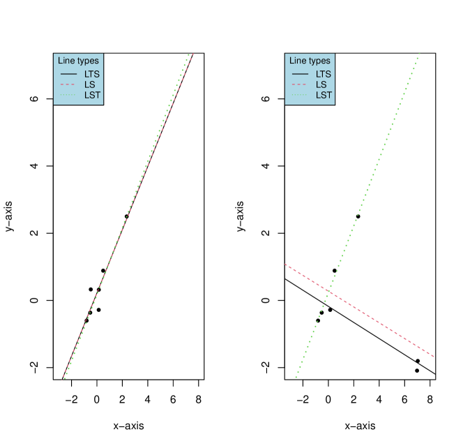
Figure 1: Left panel: plot of seven highly correlated normal points (with mean being the zero vector and covariance matrix with diagonal entries being one and off-diagonal entries being 0.88) and three lines given by the LST, the LTS, and the LS. Right panel: The LTS line (solid black) and the LST line (dotted green), and the LS (dashed red) for the same seven highly correlated normal points but with two points contaminated nevertheless. The LS line and the LTS line are identical and drastically changed due to the two points’ contamination.

Example 1 (Small illustrating bivariate data sets). To take the advantage of graphical illustration of data sets and plots, we start with $p=2$, the simple linear regression case.

We generate seven highly correlated bivariate normal points with zero mean vector and $0.88$ as the correlation between $x$ and $y$ (the scatterplot of data points is given in the left panel of Figure 1). Two out of seven points are adversarially contaminated in the right panel of the Figure. Three lines are fitted to the data sets. Inspecting the Figure reveals that (i) all lines catch the overall linear pattern for perfect highly correlated normal points in left panel; (ii) when there are ($28.6\%$) contamination, the line LTS, parallel to the LS, is drastically attached by the two outliers. This is not the case for the line of LST, which resist the contamination (outliers). Note that, theoretically speaking, both LTS and LST can resist, asymptotically, up to $50\%$ contamination without breakdown, see [6] and [16]. One might argue that this example is not representative for LTS line since the data set is too small. To meet such concern, a similar instance is given in Figure 2 with sample size $80$.

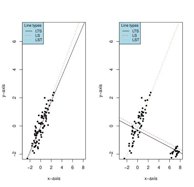
Figure 2: $80$ highly correlated normal points with $30\%$ of them are contaminated by other normal points. Left: scatterplot of the uncontaminated data set and three lines . Right: LTS, LST, and LS lines. Solid black is LTS line, dotted green is the LST, and dashed red is given by the LS - parallel to LTS line in this case.

Example 2 (Pure Gaussian data sets) The classical least squares estimator, albeit is sensitive to outliers as shown above, performs the best for pure Gaussian data sets. Now we investigate the efficiency of the LTS and LST with respect to the LS in the pure Gaussian data sets scenario.

For a general regression estimator $\mathbf{t}$, We calculate $\mbox{EMSE}:=\sum_{i=1}^{R}\|\mathbf{t}_{i}-\boldsymbol{\beta}_{0}\|^{2}/R$, the empirical mean squared error (EMSE) for $\mathbf{t}$. if $\mathbf{t}$ is regression equivariant (see [6] or [12, 14] for definition), then we can assume (w.l.o.g.) that the true parameter $\boldsymbol{\beta}_{0}=\mathbf{0}\in\mathbb{R}^{p}$ (see [13, 16], [6]). Here $\mathbf{t}_{i}$ is the realization of $\mathbf{t}$ obtained from the ith sample with size $n$ and dimension $p$, and replication number $R$ is usually set to be $1000$. Meanwhile, we also calculate the sample variance of $\boldsymbol{t}$, by $\mbox{SVAR}(\boldsymbol{t}):=\sum_{i=1}^{R}\|\mathbf{t}_{i}-\bar{\boldsymbol{t}}\|^{2}/(R-1)$, where $\bar{\boldsymbol{t}}$ is the mean of all $\{\boldsymbol{t}_{i},i\in\{1,2,\cdots,R\}\}$, and obtain the finite sample relative efficiency (RE) of a procedure (denoted by P) with respect to the LS by the ratio of $\mbox{RE}(P):=\mbox{SVAR}(\widehat{\boldsymbol{\beta}}_{ls})/\mbox{SVAR}(\widehat{\boldsymbol{\beta}}_{P})$. At the same time, we record the total time (TT) consumed by different procedures for all replications. Simulation results are listed in Table 1.

Pure Gaussian data sets

n	method	EMSE	SVAR	TT	RE	EMSE	SVAR	TT	RE
			p=5				p=10
	LTS	0.3067	0.0696	25.985	0.5994	0.3017	0.1934	49.399	0.5393
100	LST	0.2787	0.0419	11.799	0.9954	0.2128	0.1042	10.596	1.0008
	LS	0.2786	0.0417	1.4166	1.0000	0.2128	0.1043	1.3384	1.0000
	LTS	0.2674	0.0300	41.750	0.6678	0.1825	0.0741	87.448	0.6493
200	LST	0.2577	0.0203	28.037	0.9869	0.1567	0.0482	28.490	0.9984
	LS	0.2574	0.0200	1.2762	1.0000	0.1564	0.0481	1.3128	1.0000
			p=20				p=30
	LTS	0.5351	0.4828	159.62	0.4984	0.9656	0.9311	354.59	0.4468
100	LST	0.2919	0.2397	10.824	1.0036	0.4496	0.4153	11.594	1.0018
	LS	0.2927	0.2406	1.3827	1.0000	0.4503	0.4161	1.4382	1.0000
	LTS	0.2219	0.1700	264.20	0.6275	0.3298	0.2956	572.32	0.5824
200	LST	0.1583	0.1063	27.969	1.0031	0.2060	0.1717	27.638	1.0025
	LS	0.1587	0.1067	1.4514	1.0000	0.2064	0.1721	1.6345	1.0000

Table 1: EMSE, SVAR, TT (seconds), and RE for LTS, LST, and LS based on $1000$ standard Gaussian samples for various $n$s and $p$s.

Inspecting the Table 1 reveals some stunning findings (i) the LS is by far the fastest procedure followed by LST, LTS is the slowest. It, however, is no longer the most efficient even in the pure Gaussian data points setting, the LST can be as efficient as or even more efficient than the LS. (ii) the LST is not only faster than LTS but also possesses a smaller EMSE and SVAR than LTS in all cases considered. As a pure R based procedure, it could speed up by an order of magnitude if employing C++, Rcpp, or Fortran programming language just like LS or LTS does. (iii) the LTS is not efficient nor the fastest, in fact, it is the least efficient, its RE could be as low as $45\%$, which is consistent with its asymptotic efficiency that has been reported to be just $7\%$ in [9] or $8\%$ in [3] (page 132) in the literature. Example 3 (Contaminated Gaussian data sets) Pure Gaussian points are rare in practice. More realistic is contaminated (or mixed) Gaussian points. We now investigate the robustness of three procedures against the contamination (or outliers). We generate $1000$ samples $\{\mathbf{z}_{i}=(\boldsymbol{x^{\top}_{i}},y_{i})^{\top},i\in\{1,\cdots,n\}\}$ with various $n$s from the normal distribution ${N}(\boldsymbol{\mu},\boldsymbol{\Sigma})$, where $\boldsymbol{\mu}$ is a zero-vector in $\mathbb{R}^{p}$, and $\boldsymbol{\Sigma}$ is a $p$ by $p$ matrix with diagonal entries being $1$ and off-diagonal entries being $0.9$. Then $\varepsilon\%$ of them are contaminated by $m=\lceil n\varepsilon\rceil$ points, where $\lceil\cdot\rceil$ is the ceiling function. We randomly select $m$ points of $\{\boldsymbol{z}_{i}$, $i\in\{1,\cdots,n\}\}$ and replace them by $(7,7,\cdots,7,-7)^{\top}$. We apply the three methods to the contaminated data sets, simulation results are displayed in Table 2.

Gaussian data sets each with $\varepsilon$ contamination rate

method	EMSE	SVAR	TT	RE	EMSE	SVAR	TT	RE
	p=5	n=50	$\varepsilon=5\%$		p=5	n=50	$\varepsilon=10\%$
LTS	0.3948	0.1587	17.505	8.510	0.3756	0.1386	16.720	15.152
LST	0.3329	0.0966	7.8941	13.977	0.3363	0.0989	9.3230	21.220
LS	1.4223	1.3504	1.4720	1.0000	2.2726	2.0997	1.4459	1.0000
	p=5	n=100	$\varepsilon=5\%$		p=5	n=100	$\varepsilon=10\%$
LTS	0.2986	0.0616	25.368	12.033	0.2966	0.0595	25.201	17.132
LST	0.2798	0.0428	13.552	17.323	0.2849	0.0478	14.651	21.308
LS	0.8328	0.7410	1.6931	1.0000	1.1827	1.0189	1.3112	1.0000
	p=10	n=100	$\varepsilon=20\%$		p=10	n=100	$\varepsilon=30\%$
LTS	0.2568	0.1484	56.156	24.994	42.140	42.023	63.621	0.1083
LST	0.2426	0.1343	18.208	27.629	0.2583	0.1498	22.538	30.375
LS	3.8447	3.7099	1.2891	1.0000	4.6918	4.5500	1.2452	1.0000
	p=10	n=200	$\varepsilon=20\%$		p=10	n=200	$\varepsilon=30\%$
LTS	0.1725	0.0641	96.346	26.817	10.129	10.119	105.66	0.2043
LST	0.1683	0.0599	46.430	28.706	0.1799	0.0715	51.175	28.927
LS	1.8479	1.7191	1.3379	1.0000	2.2121	2.0668	1.2854	1.0000
	p=20	n=100	$\varepsilon=20\%$		p=20	n=100	$\varepsilon=30\%$
LTS	0.6643	0.6140	282.17	15.798	145.26	145.14	889.92	0.0864
LST	0.3748	0.3229	21.219	30.040	0.4412	0.3891	24.046	32.233
LS	9.7959	9.7001	1.3300	1.0000	12.644	12.541	1.3221	1.0000
	p=20	n=200	$\varepsilon=20\%$		p=20	n=200	$\varepsilon=30\%$
LTS	0.1963	0.1443	403.66	29.050	31.777	31.760	850.31	0.1597
LST	0.1860	0.1340	47.643	31.283	0.2109	0.1588	61.292	31.946
LS	4.2849	4.1915	1.5260	1.0000	5.1678	5.0730	1.4555	1.0000

Table 2: EMSE, SVAR, TT (seconds), and RE for LTS, LST, and LS based on $1000$ standard Gaussian samples for various $n$s and $p$s.

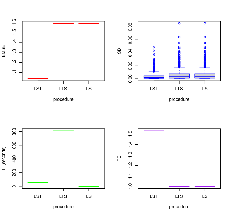
Figure 3: Performance of three procedures with respective $1000$ normal samples (points are highly correlated) with $p=30$ and $n=300$, each sample suffers $0\%$ contamination.

Inspecting the Table reveals that (i) no one can run faster than LS; LST is not only always faster but also more efficient than LTS. (ii) With small contamination, LS is almost always the least efficient estimator with the exception when the contamination rate reaches $30\%$. In the latter case, LTS shockingly becomes the least efficient. In the theory, both LTS and LST can resist, asymptotically, up to $50\%$ contamination without breakdown (see p. 132 of [6], and [13, 16]). However, the performance of LTS is frustrating when there is $30\%$ contamination.

Example 4 (Performance when $\boldsymbol{\beta}^{0}$ is given). In the calculation of EMSE above, we assumes that $\boldsymbol{\beta}^{0}=\boldsymbol{0}$ in light of regression equivariance of an estimator $\boldsymbol{t}$. In this example, we will provide $\boldsymbol{\beta}^{0}$ (for convenience write it as $\boldsymbol{\beta}_{0}$) and calculate $y_{i}$ using the formula $y_{i}=(1,\boldsymbol{x}^{\top}_{i})\boldsymbol{\beta}^{\top}_{0}+e_{i}$, where we simulate $\boldsymbol{x}_{i}$ from a standard normal distribution with zero mean vector and identical covariance matrix. $e_{i}$s are i.i.d. follow a standard normal distribution.

We set $p=30$, $n=300$ and a $\boldsymbol{\beta}_{0}$ with its first 15 component being $1$ and the last 15 component being $-1$. There is a $0\%$ or $5\%$ contamination for each of $1000$ normal samples (generated as in Example 3) with the contamination scheme as: we randomly select $m=\lceil n\varepsilon\rceil$ points out of $\{\boldsymbol{z}_{i}$, $i\in\{1,\cdots,n\}\}$ and replace them by $(4,4,\cdots,4,-4)^{\top}$. We then calculate the squared deviation (SD) $(\widehat{\boldsymbol{\beta}}_{i}-\boldsymbol{\beta}_{0})^{2}$ for each sample, the total time consumed by each procedures for all $1000$ samples, and the relative efficiency (the ratio of EMSE of LS versus EMSE of a procedure). The four performance criteria for different procedures are displayed graphically via boxplot in Figures 3 and 4 and numerically via Table 3.

$1000$ samples $\{(\boldsymbol{x}^{\top}_{i},y_{i})^{\top}\}$ with $y_{i}=(1,\boldsymbol{x}^{\top}_{i})\boldsymbol{\beta}^{\top}_{0}+e_{i}$, $\boldsymbol{x}_{i}\sim N(0_{p\times 1},I_{p\times p})$, $e_{i}\sim N(0,1)$

(n,  p)	procedure	EMSE	SVAR	TT	RE
			$\varepsilon=0\%$
	LTS	1.5745	1.5735	859.56	1.0000
(300, 30)	LST	1.0346	1.0333	68.241	1.5218
	LS	1.5745	1.0312	2.0217	1.0000
			$\varepsilon=5\%$
	LTS	2.1809	2.1791	874.42	1.0000
(300, 30)	LST	1.0966	1.0968	92.306	1.9888
	LS	2.1809	1.1066	2.0430	1.0000

Table 3: EMSE, SVAR, TT (seconds), and RE for LTS, LST, and LS based on $1000$ standard Gaussian samples, $0\%$ or $5\%$ of each sample is contaminated.

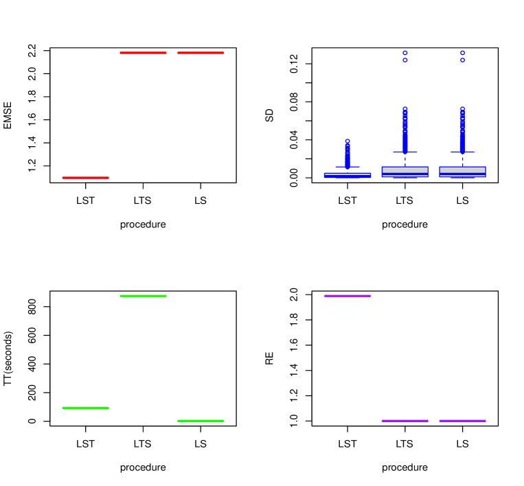
Figure 4: Performance of three procedures with respective $1000$ normal samples (points are highly correlated) with $p=30$ and $n=300$, each sample suffers $5\%$ contamination.

Inspecting the Figures and Table reveals that (i) In terms of EMSE, LST is the best while LTS and LS are almost identically lousy. (ii) In terms of SD (see Figures 3 and 4), the situation is the same as the EMSE case, i.e. LST is the best while LTS and LS are almost identically inferior. (iii) In terms of computation speed, LS is by far the best and LTS is the worst. (iv) In terms of relative efficiency, LST again is the best (this is shockingly true even for $0\%$ contamination case), and LTS and LS form the second tier. Example 5 (Performance for large real data sets)    We consider three real data sets below. For more detailed description of data sets, see http://lib.stat.cmu.edu/datasets/ (i) Plasma Retinol (PR) [4]. This data set contains 315 observations on 14 variables. The goal is to investigate the relationship between personal characteristics and dietary factors, and plasma concentrations of retinol (response), beta-carotene, and other carotenoids. (ii) PM10 The data are a subsample of 500 observations from a data set that originate in a study where air pollution at a road is related to traffic volume and meteorological variables, collected by the Norwegian Public Roads Administration. The response variable (column 1) consist of hourly values of the logarithm of the concentration of PM10 (particles), measured at Alnabru in Oslo, Norway, between October 2001 and August 2003. The predictor variables (columns 2 to 8) are the logarithm of the number of cars per hour, temperature $2$ meter above ground (degree C), wind speed (meters/second), the temperature difference between $25$ and $2$ meters above ground (degree C), wind direction (degrees between 0 and 360), hour of day and day number from October 1. 2001. (iii) NO2 This data set is collected by the same agency at the same time period as (ii) above with the same predictor variables. The only difference is that the response variable becomes hourly values of the logarithm of the concentration of NO2 (particles).We fit the data sets with the three procedures. Since some methods depend on randomness, so we run the computation R$=1000$ times to alleviate the randomness. To evaluate the performance of the three procedures, (i) we calculate the total time consumed (in seconds) for all replications for each method, (ii) the EMSE (with true $\boldsymbol{\beta}_{0}$ being replaced by the sample mean of R $\widehat{\boldsymbol{\beta}}$s from (i)), which then is the sample variance of all $\widehat{\boldsymbol{\beta}}$s up to a constant factor. (iii) we calculate the finite sample relative efficiency (RE) by the ratio of EMSE of LS to EMSE of a procedure (in the numerator being zero and denominator also being zero case, RE is defined to be $100\%$ since the procedure is as efficient as the LS). The results are reported in Table 4.

dataset	(n,  p)	procedure	EMSE	TT	RE
		LTS	2241.5	78.814	0%
PR	(315, 13)	LST	0.0000	108.09	100%
		LS	0.0000	1.4037	100%
		LTS	0.0011	152.63	0%
PM10	(500, 7)	LST	0.0000	143.57	100%
		LS	0.0000	1.4365	100%
		LTS	0.0017	150.40	0%
NO2	(500, 7)	LST	0.0000	141.72	100%
		LS	0.0000	1.3968	100%

Table 4: Total time consumed (in seconds), RE, and sample variance (EMSE) in 1000 replications by LTS, LST, and LS for three real data sets with various sample size $n$s and dimension $p$s.

Inspecting the Table reveals that (i) in terms of sample variance (or EMSE), LTS is the overall loser with the largest (non-zero) EMSE in all cases considered whereas LST and LS are the overall winner with a zero sample variance in all cases as expected (intuitively, each procedure should yield the same result for the same data set from each replication, but this is not the case for the LTS); (ii) in terms of speed, LS is the overall winner whereas LST in two out of three cases is faster than LTS; (iii) in terms of relative efficiency, LST is as efficient as the LS whereas LTS has the worst efficiency, $0\%$. $\square$

5 Concluding remarks

Is it possible to have a procedure that is as robust as the benchmark of robust regression, the LTS, meanwhile is more efficient and runs faster than the LTS? Is it possible to have a procedure that is as efficient as (or even more efficient than) the LS in the errors that are uncorrelated with mean zero and homoscedastic with finite variance scenario? It was commonly believed that the answers to these questions were certainly impossible until this article. The latter, however, has presented promising affirmative answers. In fact, it has been proved theoretically in [16] that the least squares of depth trimmed (LST) residuals regression could serve as a robust alternative to the least squares (LS) regression and a formidable competitor to the LTS regression. This article has verified the assertion empirically via concrete examples. The computation speed of the LST could be enhanced if adopting the C++, or Rcpp, or Fortran computation language.

Supplementary Materials The supplementary material for this article includes the following: (A) R code for LST regression (lstReg), (B) R code for examples 1, 2, 3, 4, and 5. (All are downloadable at https://github.com/left-github-4-codes/amlst). AcknowledgmentsThe author thanks Prof. Wei Shao for insightful comments and stimulus discussions.

Disclosure Statement The author reports there are no competing interests to declare.

FundingThis author declares that there is no funding received for this study.

ORCIDYijun Zuo: https://orcid.org/0000-0002-6111-3848

References

- [1] Donoho, D. L. (1982), “Breakdown properties of multivariate location estimators”. PhD Qualifying paper, Harvard Univ.
- [2] Donoho, D. L., and Gasko, M. (1992), “Breakdown properties of multivariate location parameters and dispersion matrices”, Ann. Statist. 20, 1803-1827.
- [3] Maronna, R. A., Martin, R. D., and Yohai, V. J.(2006), “ Robust Statistics: Theory and Methods”, John Wiley &Sons
- [4] Nierenberg DW, Stukel TA, Baron JA, Dain BJ, Greenberg ER(1989), “Determinants of plasma levels of beta-carotene and retinol”, American Journal of Epidemiology 130:511-521.
- [5] Rousseeuw, P. J. (1984), “Least median of squares regression”, J. Amer. Statist. Assoc. 79, 871-880.
- [6] Rousseeuw, P.J., and Leroy, A. (1987), Robust regression and outlier detection. Wiley New York.
- [7] Rousseeuw, P. J., Struyf, A. (1998), “Computing location depth and regression depth in higher dimensions”, Statistics and Computing, 8:193-203.
- [8] Stahel, W. A. (1981), Robuste Schatzungen: Infinitesimale Optimalitiit und Schiitzungen von Kovarianzmatrizen. Ph.D. dissertation, ETH, Zurich.
- [9] Stromberg, A. J., Hawkins, D. M., and Hössjer, O. (2000), “The Least Trimmed Differences Regression Estimator and Alternatives”, J. Amer. Statist. Assoc., 95, 853-864.
- [10] Zuo, Y. (2003) “Projection-based depth functions and associated medians”, Ann. Statist., 31, 1460-1490.
- [11] Zuo, Y. (2006), “Multi-dimensional trimming based on projection depth”, Ann. Statist., 34(5), 2211-2251.
- [12] Zuo, Y. (2021a), “On general notions of depth for regression” Statistical Science 2021, Vol. 36, No. 1, 142–157, arXiv:1805.02046.
- [13] Zuo, Y. (2021b), “Robustness of the deepest projection regression depth functional”, Statistical Papers, vol. 62(3), pages 1167-1193.
- [14] Zuo, Y. (2023), “Non-asymptotic robustness analysis of regression depth median”, Journal of Multivariate Analysis, https://doi.org/10.1016/j.jmva.2023.105247, arXiv: 2009.00646
- [15] Zuo, Y., Serfling, R., (2000), “General notions of statistical depth function”, Ann. Statist., 28, 461-482.
- [16] Zuo, Y. and Zuo, H. (2023), “Least sum of squares of trimmed residuals regression”, Electronic Journal of Statistics, Vol. 17, No. 2, 2416-2446. arXiv:2202.10329.