A Distributed ADMM-based Deep Learning Approach for Thermal Control in Multi-Zone Buildings
Abstract
The surge in electricity use, coupled with the dependency on intermittent renewable energy sources, poses significant hurdles to effectively managing power grids, particularly during times of peak demand. Demand Response programs and energy conservation measures are essential to operate energy grids while ensuring a responsible use of our resources This research combines distributed optimization using ADMM with Deep Learning models to plan indoor temperature setpoints effectively. A two-layer hierarchical structure is used, with a central building coordinator at the upper layer and local controllers at the thermal zone layer. The coordinator must limit the building’s maximum power by translating the building’s total power to local power targets for each zone. Local controllers can modify the temperature setpoints to meet the local power targets. The resulting control algorithm, called Distributed Planning Networks, is designed to be both adaptable and scalable to many types of buildings, tackling two of the main challenges in the development of such systems. The proposed approach is tested on an 18-zone building modeled in EnergyPlus. The algorithm successfully manages Demand Response peak events.
Note to Practitioners
This article addresses the problems faced by multizone buildings in maintaining thermal comfort while participating in Demand Response events. A centralized control approach is nonscalable, raises privacy concerns, and requires huge communication bandwidth. This work introduces a distributed algorithm that adapts the temperature setpoints of multi-zone buildings to enhance Demand Response participation and energy conservation. The proposed approach is fully data-driven and only requires historical data on weather, indoor temperature, and HVAC power consumption. The blueprint of the building and details about the HVAC system’s architecture are not needed. Energy savings will be spread across all the zones depending on the user’s choice of comfort temperature interval for each zone. The distributed optimization makes the approach scalable to large buildings with multiple zones. The algorithm is designed to work for buildings with various insulated zones such as apartment buildings and hotels, and may be extended to other types of buildings.
Index Terms:
Deep Learning, Distributed Optimization, ADMM, Demand Response, HVAC, BuildingsThis work has been submitted to the IEEE for possible publication. Copyright may be transferred without notice, after which this version may no longer be accessible.
I Introduction
Buildings account for approximately of the energy consumption worldwide. More than half of the building’s energy is used to maintain the occupant’s comfort, mainly through Heating, Ventilation and Air Conditioning (HVAC) systems [1]. Buildings are powerful pillars for integrating energy efficiency and Demand Response (DR) measures to reduce electricity consumption, especially during unstable power supply and peak periods. Many paths are investigated to benefit grid management by leveraging the building’s power consumption. Local Renewable Energy Sources, Energy Storage Systems, and Electric Vehicles can now be embedded in the Building Energy Management System (BEMS) to form a building-integrated microgrid [2, 3]. Efforts are also made to improve insulation materials and directly reduce the energy needs for heating and cooling purposes [4]. In addition, many grid operators are now proposing DR programs to encourage consumers to reduce their energy consumption following an incentive-based or dynamic pricing program. In both cases, they propose rewards to the end-users in exchange for reductions in their power or energy consumption, especially during periods of high solicitation of the grid. Thus, smart control of the building loads may result in substantial financial advantages for the consumers while providing support for an efficient grid operation [5, 6, 7]. Heating and cooling demands can significantly impact the total building’s power consumption profile. The thermal inertia of the building offers enhanced operational flexibility to reduce/shift a part of the load using pre-cooling or pre-heating strategies. The use of smart temperature controllers, accounting for occupancy and weather variations, results in a direct reduction of energy usage. However, it has a direct impact on the user’s comfort that must be preserved [5]. Many works have focused on the creation of advanced BEMS for monitoring and controlling a building’s energy requirements, including smart temperature controllers. Two of the main approaches used to develop BEMS are Model Predictive Control (MPC) and Reinforcement Learning (RL). For instance, [8, 9, 10] apply MPC to manage energy consumption and comfort in commercial and residential buildings. Works such as [11, 12, 13, 14, 15] use RL to create efficient and adaptive controllers for BEMS.
Optimization problems solved using MPC or RL are often formulated as centralized problems. In centralized problems, a single entity computes the solution to the problem and takes all the decisions. Centralized problem formulations for BEMS are further described in [16]. Although simple conceptually, this approach is not scalable as the system size grows [17]. Furthermore, the necessary communications between local actuators and the central controller may raise privacy concerns and failure risks. Thus, distributed architectures are increasingly considered. Distributed architectures are of two types: the hierarchical approach and the fully distributed approach (peer-to-peer). In both approaches, the complex global optimization problem is decomposed into subproblems. In hierarchical structures, the problem is solved through a coordinator who takes global decisions and communicates with Local Controllers (LCs). In fully distributed architectures, LCs directly communicate with each other to coordinate their actions. The choice of architecture is problem dependent, as each architecture has pros and cons and highly depends on the communication infrastructure [18, 11].
Distributed architectures have been increasingly used along with the Alternating Direction Method of Multipliers (ADMM) to tackle energy management challenges at the scale of the building. MPC is often considered to solve the optimization problems resulting from a decomposition, yielding a class of algorithms called Distributed Model Predictive Control (DMPC). Works using DMPC for HVAC control are further discussed in [16]. For instance, [19, 20] present case studies with linearized building dynamics, where DMPC provides equivalent performances as centralized MPC while requiring fewer computational resources. In [21], Wang et al. use a multiple-layer distributed architecture to operate HVAC systems. Their model accounts for complex coupling dynamics between the components of the HVAC system. The focus of their study is more on optimizing the operation of HVAC systems given comfort requirements. The control of the zones’ temperature setpoints to act on the power consumption has not been considered. In addition, the authors used simple linear models for the thermal dynamics of the building. In their study, Mork et al. [22] successfully implement nonlinear DMPC to control a multi-zone building. Non-linear models are seldom used in the literature but are more precise because the thermal transfer processes are non-linear [22, 23]. They use a physics-based model developed in Modelica, that accounts for the thermal and hydraulic coupling between zones. Their case studies show the efficiency of the distributed approach over centralized control. One drawback of their approach is that it requires enough knowledge about the building’s blueprint to build the model. Some data required for modelling the coupling between zones, such as door and shading positions, might also be hard to access. In addition, they apply ADMM to non-convex problems without analyzing the convergence properties of their algorithm.
On the theoretical side, ADMM is proven to converge when the underlying problem is convex [24], which is not the case in BEMS applications. To rely on the convergence guarantees of convex problems, many works linearize the dynamics of their system [19, 20, 25, 26, 27, 28]. Others rely on the empirical robustness of ADMM when applied to non-convex problems [22]. Few theoretical results exist on the convergence of ADMM in non-convex settings [29, 30]. The use of a non-convex ADMM allows to consider models more sophisticated than linear ones. In particular, models relying on Neural Networks proved to be extremely accurate to forecast the energy consumption in buildings [31, 23]. Recurrent State Space Models (RSSM) also proved to be extremely accurate to model stochastic environments and are yet to be applied to building energy forecasting. Such models, along with planning algorithms provide state-of-the-art results in many benchmark control tasks [32, 33].
In line with the International Energy Agency’s (IEA) recommendations [34], the present study focuses on the critical role of widening temperature setpoints as a way for significant energy savings and effective implementation of DR programs. While optimizing the HVAC system’s operation to efficiently track a setpoint is important, it is crucial to note that for a given temperature setpoint, there exists an inherent physical constraint on the extent of energy reduction achievable solely through the optimization of HVAC system operations. Further energy reduction may only be achieved by altering the setpoint itself. This study thus uses temperature setpoints as actuators for power consumption regulation. Within the proposed framework, users select a preferred temperature setpoint and define an associated comfort range for each zone within a building. The BEMS dynamically adjusts the setpoints within the comfort intervals to distribute energy savings across the building.
Our approach combines the recent advancement in non-convex ADMM algorithms, with state-of-the-art control methods based on Deep Learning models. First, we formulate the temperature control problem as a centralized problem with a constraint on the building’s total power consumption. Then, we convert this problem into a non-convex consensus problem that we decompose using the ADMM algorithm. We provide convergence proof of the algorithm for this non-convex setting, which is key to accurately account for the non-linear dynamics of buildings. From this formulation, we derive a surrogate problem that can be efficiently solved in practice. We test both RSSM and SSM to model the building’s zone. The models are used to plan for the temperature setpoints that best match the comfort requirements of zones while enforcing a limit on the building’s power usage. The two models are compared in terms of prediction accuracy to benchmark RSSM in a building environment, and in terms of control quality to assess the performance of our distributed control framework. The main contributions of this study are summarized as follows:
-
1.
This work proposes an efficient algorithm to adjust a building’s indoor temperature based on available energy resources. The approach contributes to energy conservation while minimally affecting occupant comfort, making it a valuable asset for DR.
-
2.
We combine non-convex ADMM and advanced, fully data-driven, Deep Learning models to provide a distributed control for HVAC systems. To the best of our knowledge, this is the first work combining non-linear Deep Learning models and ADMM.
-
3.
While the global constraint is on the power consumption of the building, we propose to use temperature setpoints of the zones as actuators. Therefore, no assumption is made on the type of HVAC system, which makes our approach easily adaptable from one building to another.
-
4.
The building is modeled using a fully data-driven approach, where no prior knowledge about the building’s blueprint is required. The RSSM allows one to plan in a stochastic environment and handle uncertainties in a robust MPC framework. The SSM can be used in computationally efficient shooting controllers.
-
5.
We propose a convergence analysis for our non-convex ADMM algorithm. A case study shows the good convergence properties of our algorithm in practice.
II Problem formulation
In this study, a building composed of thermal zones is considered. Each zone has a temperature control system, i.e. a device like a PID or ON/OFF controller able to track a local temperature setpoint. Specifically, we consider a discretized setting, where occupants choose temperature setpoints for each zone, that are optimal for their comfort. These setpoints may vary in time but are known beforehand. At time for the zone , represents the power consumption of a Heating or Cooling (HC) system.
The power consumption is closely related to the temperature setpoints [35]. One can act on the setpoints to control the building’s HC power consumption below a maximum value. To this purpose, the global power constraint must be distributed to local temperature controllers acting on each zone, and translated to temperature setpoints.
The proposed control system modifies the occupants’ setpoints by , so that the setpoint tracked by the HC system is at time is zone . Let
be a vector containing the setpoint changes for all the zones on a horizon of timesteps. Let be the vector containing all setpoint changes at time . Similarly, contains all the temperature setpoint changes for zone over the horizon. This indexing convention will be used for other vectors as well. In particular, the vector of power consumption:
The optimal setpoint changes are solutions to the following optimization problem:
[3] Δ∥Δ∥^2_2 \addConstraints_t+1, i = f_i (s_t,i, δ_t,i, s_y, j ∈N_i, δ_t,j ∈N_i ), ∀t,i \addConstraint—δ_t,i— ≤M_i, ∀t,i \addConstraintA u ≤P^max
where
-
•
represents the dynamics of zone ,
-
•
is the state of zone . The state includes, in particular, , the air temperature, and the HC power consumption. The state is partially observable as it may also include the temperature of the walls or the thermal capacity of the zone.
-
•
is the set of neighbors of zone ,
-
•
is a matrix that sums the power consumption of all the zones at each timestep. For instance, for two zones and a horizon of two timesteps:
The coefficient selects the power consumption of zone at the first time step.
-
•
is a vector containing the maximum power for each timestep. The vector inequality in eq. (II) is component-wise.
-
•
is the maximum setpoint change defined by the occupants in zone .
To solve this problem efficiently, we reformulate it as a sharing problem [29] and apply ADMM.
First, the inequality constraint (II) is relaxed using a new parameter such that . This ensures the problem is feasible and removes a coupling constraint. Second, the true dynamics is approximated by a function that does not take the neighboring states as input. This assumption implies that one can reasonably predict a zone’s state without having to predict the states of neighboring zones. Note that the initial state of a zone , may still be augmented to include information about the neighbors at . In many buildings such as hotels, offices, or residential buildings, the temperature ranges in the zones are similar, thus limiting the heat exchanges. We will assess this assumption experimentally in section V to show that it is reasonable if the zones are well insulated. Such an assumption is also discussed in [22, 36]. The optimization problem becomes:
[3] Δ∥ Δ∥^2_2 + ∥Au - P^tot∥^2_2 \addConstraints_t+1, i = q_i (s_t,i, δ_t,i ), ∀t,i \addConstraint—δ_t,i— ≤M_i, ∀t,i
The HC power consumption is now driven towards the parameters . The choice of is important and will be further discussed in section V.
Let us define a function that maps the state of a zone to its power usage:
Given the setpoints and the first state, future states are computed by unrolling the dynamics:
To ease the notations, we define the following functions, for all and :
| (1) | |||
| (2) | |||
| (3) |
The index to the function indicates that it represents the state at time of zone computed from . Only the first elements of are needed to compute , but the entire vector is passed for notational simplicity. The power usage becomes:
| (4) |
and we construct the following problem: {mini!}[3] Δ∑_i=1^N g( Δ_i) + ℓ( Δ) \addConstraint—δ_t,i— ≤M_i ∀t,i
This problem is a sharing problem as described in [29]. Each zone has a local objective represented by and a global objective represented by . The total power available is a common resource that must be shared across all zones to satisfy the local comfort requirements.
We introduce duplicated variables and form an equivalent problem with vector linear equality constraints: {mini!}[3] Δ∑_i=1^N g( Δ_i) + ℓ(∑_i=1^N B_i ¯Δ_i ) \addConstraint¯Δ_i = Δ_i ∀i \addConstraint—δ_t,i— ≤M_i ∀t,i
The matrices for are such that . The augmented Lagrangian, with Lagrange multipliers associated with the equality constraints, is:
| (5) |
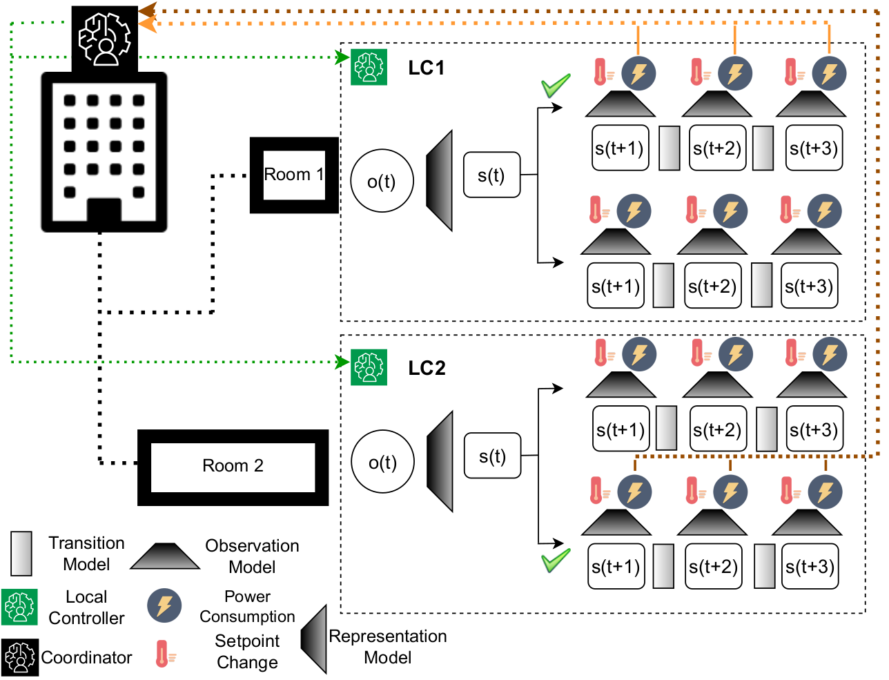
The sharing problem can be solved using Alg. 1. We distinguish two main sub-problems in this algorithm. The first one is the local controller problem (line 5) and the second one is the coordinator problem (line 7).
As stated in the following theorem, under some Lipschitz regularity assumptions and the right choice of , this algorithm is guaranteed to converge although the problem is not convex. We will assess the quality of the solutions experimentally in section V.
Theorem II.1.
where is the set of primal-dual stationary solutions of the problem.
Evaluating the models of each dynamics is computationally expensive. To leverage the benefits of the decomposition, the models’ evaluation should be placed in the for loop and computed in parallel. In Alg. 1 the models’ evaluation is in the function, in the coordinator problem.
We can explicit the relationship between the setpoints and the related power consumption (4) as a constraint in the LC problem.
[3] Δ_ig(Δ_i) + λ_i^T (¯u_i - u_i) + ρ—— ¯u_i - u_i ——_2^2 \addConstraintu_t,i = ϕ(Q_t,i(s_0, i, Δ_i)) \addConstraint¯u_t,i = ϕ(Q_t,i(s_0, i, ¯Δ_i)) \addConstraint—δ_t,i— ≤M_i
and consider the surrogate coordinator problem:
[3] ¯u~ℓ(¯u) + ∑_i=1^N λ_i^T (¯u_i - u_i) + ρ—— ¯u_i - u_i ——_2^2
where . This formulation may be derived from the same decomposition steps as the ones above, but using the following equation rather than eq. (4):
| (6) |
Eq. (6) bounds the state and power usage to a setpoint. The problem is that is not an injective application. For instance, if the temperature in a zone is , temperature setpoints below will all yield a heating power of . Such an application is impossible to learn accurately in practice. That said, depending on the type of setpoint tracking system, how the power is measured and the operation regime, one may find conditions for to satisfy the requirements of Theorem 1. For instance, a proportional controller that operates with a zone’s temperature around the setpoint or an ON/OFF controller used with Pulse Width Modulation would give good properties to .
Instead of enumerating such conditions, that are hard to verify in practice, we choose to provide a theoretical analysis for the problem formulation (4). This formulation is more natural and indicates the form of the ADMM decomposition for the surrogate problem. As shown in Section V, the surrogate formulation yields efficient computation and shows excellent convergence properties experimentally. In addition, it provides a good intuition about the underlying mechanism: the coordinator (i.e. problem (II.1)) is choosing the amount of power for each room and each timestep, to ensure that the power constraint is always satisfied. The LCs (i.e. problems (II.1)) must then find the temperature setpoints to track this power target while preserving the users’ comfort. Even if multiple setpoints may satisfy the constraints II.1 and II.1, the lowest setpoint changes will be chosen because of the term is the objective function.
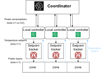
The control architecture is summarized in Fig. 1.
III Local Controllers and Zone Modelling
To successfully plan for the best setpoint changes without implementing any actions, LCs must be able to predict the evolution of the system. In this section, we present two methods for the modeling of a thermal zone: Recurrent State Space Models (RSSM) and State Space Models (SSM).
III-A Reccurent State Space Model
The RSSM is a stochastic model that allows forecasting of the power usage of each zone under uncertainties brought by many unobservable disturbances. The use of RSSM for planning is further described in [32]. In this section, we focus on some key elements for completeness.
The RSSM is a black-box model, learned from previously collected data. It is composed of three main parts:
-
1.
A representation model (encoder), which maps the observations to the latent state of the system. The use of an encoder is important because the system is partially observed. One can include lags of power and temperature in the observation to build a better representation of the state and cope with partial observability.
-
2.
A transition model, that predicts the evolution of the latent space. Note that this transition model is composed of two parts: (1) a deterministic state model which predicts the evolution of the deterministic part of the state and (2) a stochastic state model which samples the next latent state according to : . The latter part is important in our case as it accounts for the perturbations due to the occupancy and neighboring zones.
-
3.
An observation model (decoder), that outputs the observation corresponding to a given latent state.
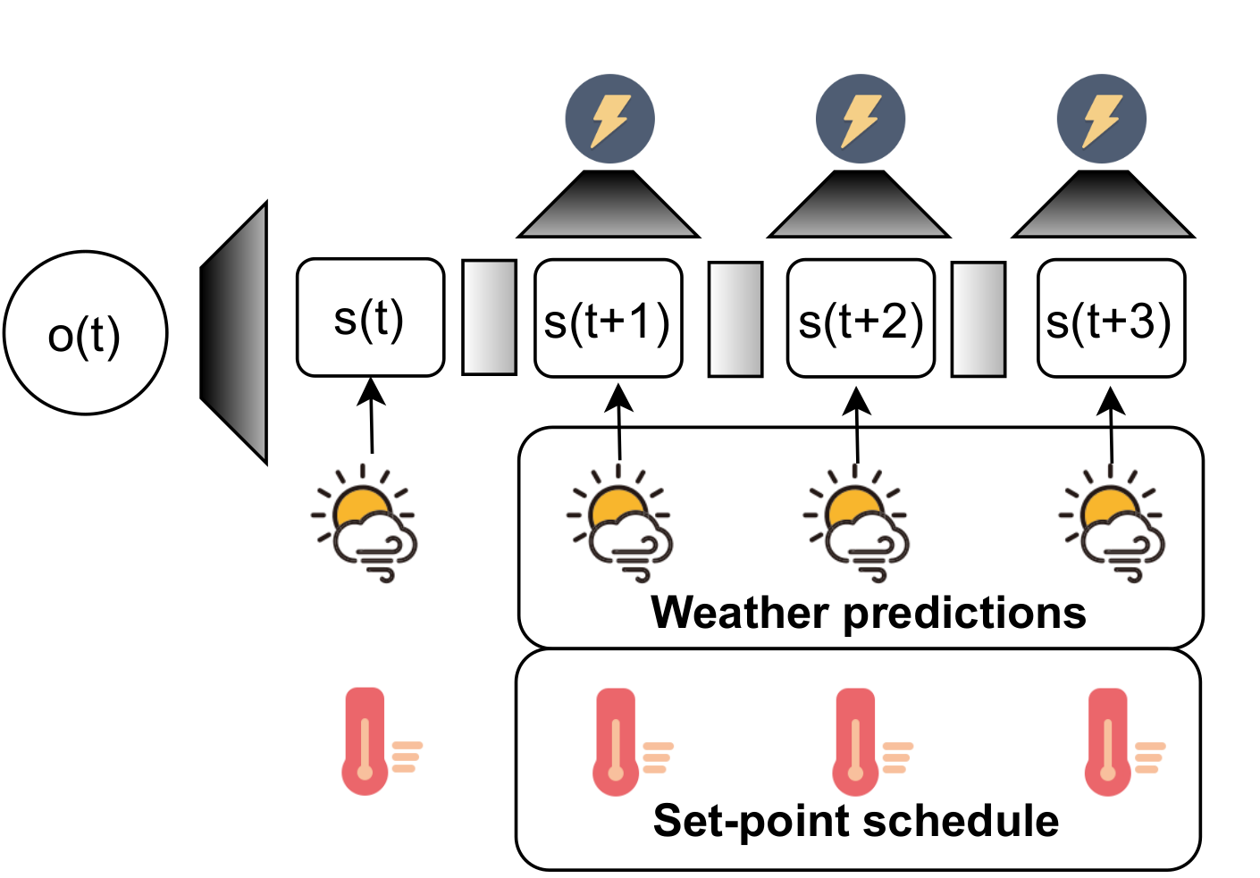
All these components are represented by neural networks. We use the same set of parameters to learn the observation model, the transition model, and the representation model. The objective is to maximize the variational bound as proposed in [32]. The transition model allows to predict one timestep ahead in the latent space. Multiple steps prediction is achieved by applying the model recursively. This is convenient as the user may want to change the prediction horizon without having to retrain the model. The latent space embeds the inner state of the room, mainly composed of the power usage and the room’s temperature. This state is influenced by exogenous perturbations such as weather and the temperature setpoint. To not overload the transition model, we do not include these disturbances in the latent space as it is usually done with this type of model. Instead, we feed the transition model with the previous latent space as well as forecasts of the disturbances, as pictured in Fig. 3. The advantages of this approach are that a single weather prediction system is required for the entire building. Since the RSSM of each zone does not have to predict the complex evolution of the weather on top of the evolution of the room’s state, it can provide better predictions using a smaller network model. In addition, some disturbances such as temperature setpoint schedules may be known beforehand and can be passed exactly to the transition model at each prediction step.
III-B State Space Models
The State Space Model (SSM) has the same structure as the RSSM, but it does not include the stochastic part. The transition model is a GRU cell that takes as input the disturbances (i.e. the weather and the setpoints). The latent state is carried by the hidden state of the GRU cell. The model is trained to minimize the mean squared error between the predicted and actual powers.
IV Distributed Planning Networks
In this section, we present how the models of each LC are combined with the coordinator using ADMM. The proposed algorithm is called Distributed Planning Networks as it embeds the idea of the Planning Networks in a distributed architecture. Fig. 2 and Alg. 3 summarize the approach.
The coordinator problem is a convex penalized least square problem. It can be solved easily with existing solvers. The challenge is more on the side of the LC problem (II.1).
To efficiently find a solution to the non-convex LC problem, we propose two approaches. The first one is a random search for the best temperature setpoints. The second one is a shooting method, where we differentiate through the prediction model and use the gradient to guide the search. Once the best setpoint changes have been found for the upcoming horizon, only the setpoint changes of the first timestep are implemented. The process is then repeated to allow for re-planning and correction of the control.
IV-A Planning by Random Search with RSSM
The random search is conducted as follows:
-
1.
Generate random sequences of setpoint changes .
-
2.
Sample the trajectories corresponding to each using the RSSM. For each , the RSSM outputs a distribution for the trajectory of states. For one choice of , multiple states trajectories may be sampled from the distribution to account for uncertainties.
-
3.
Select providing the lowest score as defined by (II.1).
While using ADMM, the steps presented above need to be repeated at each iteration. The second step is computationally expensive as it requires many forward passes in the transition and observation networks. However, only the third step depends on the ADMM iteration. To limit the computational time, the trajectories (i.e. the two first steps) are pre-computed and stored before the start of ADMM. Note that these two steps can be performed in parallel for each zone. At each ADMM iteration, the score of each trajectory is then computed from the pre-computed trajectory with respect to the current power targets .
IV-B Planing by Shooting with SSM
The SSM is fully differentiable. One can formulate the problem (II.1) as an Initial Value Problem and use single shooting to minimize the running cost given by the objective function. The equality constraints representing the dynamics are implicitly satisfied by the prediction model. To handle the inequality constraint (II.1), we use projected gradient descent to keep the setpoint changes within the desired interval. This approach assumes continuous values for the setpoints. In practice, we round the values at the resolution of the setpoint tracker of the zone afterwards. A stopping criterion on the number of decimals changing in at each iteration is used to make the approach computationally efficient.
V Results
To test the proposed approach, we use the low-rise apartment building, one of the Department Of Energy (DOE) residential reference buildings. The building is modeled in EnergyPlus, a software that provides thermal simulations for buildings with state-of-the-art accuracy. The building is composed of three floors of 6 apartments each. Apartments are equipped with independent HVAC systems, temperature setpoints schedules, occupancy schedules, and appliance usage schedules. Simulations are run using Typical Meteorological Year (TMY) files coming from the DOE climate zone 7A, representing the weather in the North-East of the United States of America and South-East of Canada. In each apartment, the user setpoint is kept constant, but may vary between and from one apartment to the other. For the purpose of this study, we are considering heating periods, and hence we modify the default HVAC systems to electric heating-only systems with an efficiency of one. The EnergyPlus timestep was set to 15 minutes. The prediction horizon is set to one or two hours and the ADMM timestep is 30 minutes, meaning we can re-plan to change the setpoints every 30 minutes.
V-A Models accuracy
| zone | RSSM | SSM | zone | RSSM | SSM | |
|---|---|---|---|---|---|---|
| 1h ahead forecast | 1 | 185 | 78 | 10 | 125 | 89 |
| 2 | 129 | 79 | 11 | 158 | 140 | |
| 3 | 181 | 88 | 12 | 127 | 71 | |
| 4 | 136 | 67 | 13 | 177 | 92 | |
| 5 | 122 | 55 | 14 | 134 | 94 | |
| 6 | 130 | 68 | 15 | 164 | 105 | |
| 7 | 137 | 94 | 16 | 152 | 69 | |
| 8 | 144 | 116 | 17 | 128 | 57 | |
| 9 | 159 | 107 | 18 | 134 | 84 | |
| zone | RSSM | SSM | zone | RSSM | SSM | |
| 2h ahead forecast | 1 | 184 | 80 | 10 | 98 | 82 |
| 2 | 120 | 71 | 11 | 144 | 133 | |
| 3 | 182 | 88 | 12 | 109 | 72 | |
| 4 | 134 | 63 | 13 | 173 | 103 | |
| 5 | 104 | 51 | 14 | 112 | 96 | |
| 6 | 127 | 66 | 15 | 159 | 110 | |
| 7 | 127 | 105 | 16 | 122 | 71 | |
| 8 | 131 | 121 | 17 | 105 | 79 | |
| 9 | 152 | 108 | 18 | 109 | 102 |
First, we test the accuracy of the prediction models. Both RSSM and SSM are trained offline for each zone of the building. The training data are generated by running simulations with random temperature setpoints changed every period of random duration, ranging from 1h to 24h. The observation of a zone contains the zone’s current temperature as well as the power consumption of each timestep for the last hour. The output of the representation model is the power consumption of the next timestep.
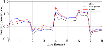
At each timestep, the zone’s observation is completed with disturbances inputs. Disturbances include the temperature setpoint and the temperature setpoint changes that are known beforehand. As one may observe in Fig. 4, the changes in the temperature setpoints cause steep variations in the power. To accurately predict these changes, a key feature added is the difference between setpoint changes from one timestep to the next i.e. . The disturbances also include the weather, composed of the outdoor temperature and solar radiation. For simplicity, we did not build a weather forecast model. Instead, we used perfect weather information and added random noise to account for prediction errors.
Table I shows the Mean Absolute Error (MAE) of each zone for one-hour and two-hours ahead forecasts. The SSM performs consistently better than the RSSM, but both methods give accurate predictions. For the entire building’s power forecast, the Mean Average Percentage Errors (MAPE) of the SSM are and for one-hour and two-hours ahead predictions. The MAPE of the RSSM are and respectively. These predictions were made without observing the states of the neighboring zones, as stated in the assumption of the model used in (II).
V-B Distributed Planning Networks and Power Control
To test the Distributed Planning Networks algorithm, we propose to implement it for peak load reduction. We consider a Demand Response (DR) program where the utility sends an early notification to the building’s operator to reduce the power demand during peak demand events. We assume that the events occur between and every morning over a period of three weeks. We also assume that this reduction implies a limit on the heating demand that should not exceed for all timesteps during DR events. For each zone, we set , with an action step of .
As mentioned in section II, translating the constraint’s parameter to (defined in eq. (II) ) is important as the building power consumption will be driven towards . To find the right , we propose to leverage the prediction model of each zone. We forecast the total power for setpoint changes of and to find lower and upper bounds on the power. If the lower bound is below , the optimal solution of the problem II is and no further computation is required. If the upper bound is above , the problem (II) is unfeasible. In the latter case, depending on the energy pricing, one could either reduce as much as possible the temperatures to lower the consumption, or take no action not to alter the comfort since the DR requirement cannot be met. If falls between the upper and lower bounds, we proceed with the Distributed Planning Networks algorithm. We then set . Note that in practice, we use a slack parameter to mitigate the effects of prediction errors, and set . This procedure is detailed in Alg. 2.
V-B1 Planning by shooting with SSM
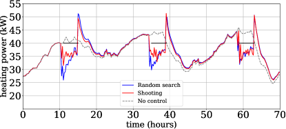
During the three week test period, the power consumption was successfully reduced below during each DR event. Fig. 5 shows the power consumption during three days of the test period.
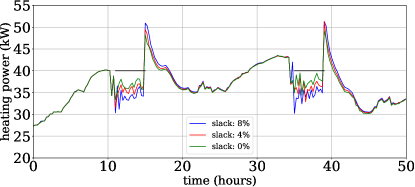
Fig. 6 shows the effect of the slack parameter on the heating power consumption. The more increases, the more conservative the control is but the higher the chance to satisfy the power constraint despite prediction errors. In our experiment, the power constraint was satisfied for the three choices , , and . However, the maximum power monitored during DR event increased as the decreased. With the power reached , compare to a maximum of around for , making the power constraint really tight. The right choice of is therefore a trade-off between comfort and power usage.
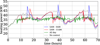
In Fig. 5, we observe rebound peaks caused by the increase of temperature setpoints after the DR events. These peaks may be managed in several ways. For instance, as shown in Fig. 7, one may extend the duration of the DR event to reduce the magnitude of the rebound peaks. Our algorithm may also be used for peak shaving by maintaining the power constraint throughout the day, as shown by the green curve in Fig. 7.
Table II shows the distribution of the temperature setpoints during active DR events. We observe that the effort is evenly spread among the zones. No zone had to take an extreme action and most of the actions are between and . Note that we did not enforce any type of fairness in the algorithm. We initialize the ADMM iterations with a setpoint change of and the same power target for every zone. We attribute this equal distribution of actions to the initialization. Differences arise because each zone has a different heating power requirement. Power consumption is influenced by many factors such as the orientation of the building, the position of the zone within the building, the presence of windows, and the occupancy.
V-B2 Planing by random search with RSSM
| SSM | zone | mean | None | Low | Medium | High | zone | mean | None | Low | Medium | High |
| 1 | -0.72 | 0 | 34.21 | 65.79 | 0 | 10 | -0.61 | 0 | 52.63 | 47.37 | 0 | |
| 2 | -0.56 | 0 | 65.79 | 34.21 | 0 | 11 | -0.74 | 0 | 44.74 | 47.36 | 7.90 | |
| 3 | -0.80 | 0 | 18.42 | 81.58 | 0 | 12 | -0.78 | 0 | 26.31 | 71.05 | 2.64 | |
| 4 | -0.73 | 0 | 34.21 | 65.79 | 0 | 13 | -0.84 | 0 | 15.79 | 78.95 | 5.26 | |
| 5 | -0.66 | 0 | 42.10 | 57.90 | 0 | 14 | -0.61 | 0 | 55.26 | 44.74 | 0 | |
| 6 | -0.78 | 0 | 21.05 | 78.95 | 0 | 15 | -0.78 | 0 | 26.32 | 71.05 | 2.63 | |
| 7 | -0.70 | 0 | 39.48 | 57.89 | 2.63 | 16 | -0.82 | 0 | 18.42 | 78.95 | 2.63 | |
| 8 | -0.66 | 0 | 50.0 | 44.73 | 5.27 | 17 | -0.79 | 0 | 21.06 | 76.31 | 2.63 | |
| 9 | -0.74 | 0 | 39.47 | 55.26 | 5.27 | 18 | -0.73 | 0 | 26.32 | 71.05 | 2.63 | |
| Model RSSM | zone | mean | None | Low | Medium | High | zone | mean | None | Low | Medium | High |
| 1 | -1.14 | 8.12 | 13.51 | 24.32 | 54.05 | 10 | -1.29 | 5.41 | 13.51 | 13.51 | 67.57 | |
| 2 | -1.27 | 2.72 | 13.51 | 24.32 | 59.45 | 11 | -1.32 | 2.70 | 8.11 | 18.92 | 70.27 | |
| 3 | -1.24 | 2.71 | 10.81 | 29.72 | 56.76 | 12 | -0.9 | 13.52 | 35.14 | 8.10 | 43.24 | |
| 4 | -1.14 | 8.12 | 8.11 | 24.32 | 59.45 | 13 | -1.17 | 8.12 | 21.62 | 13.51 | 56.75 | |
| 5 | -1.35 | 0 | 18.92 | 16.22 | 64.86 | 14 | -1.32 | 2.70 | 13.52 | 13.51 | 70.27 | |
| 6 | -1.41 | 0 | 8.11 | 13.51 | 78.38 | 15 | -0.78 | 0 | 51.35 | 16.22 | 32.43 | |
| 7 | -1.23 | 0 | 16.21 | 24.32 | 59.46 | 16 | -1.16 | 5.41 | 18.92 | 16.22 | 59.45 | |
| 8 | -1.36 | 0 | 16.22 | 10.81 | 72.97 | 17 | -1.17 | 0 | 24.33 | 21.62 | 54.05 | |
| 9 | -1.41 | 0 | 8.10 | 16.22 | 75.68 | 18 | -1.15 | 0 | 24.32 | 24.32 | 51.36 |
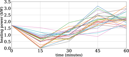
A random search is used along with the RSSM to plan for the best setpoints. We split the computational budget between exploring the action space (i.e. sampling trajectories for different ) and exploring the possible trajectories for each choice of . At the beginning of each timestep, we randomly sample 100 different choices for , and for each , we sample 25 different trajectories. We then select the trajectory out of the 25 that yields the highest power consumption, to optimize based on the worst-case scenario. Fig. 8 shows an example of different power consumptions sampled from a given state for a choice of . Note that with this approach, we fix the slack parameter to zero because the optimization is already made based on a worst-case scenario. The experiment is repeated for 5 different seeds. The results are consistent across all the seeds. For simplicity, only one outcome is presented.
Using this type of controller, the power is successfully controlled below . The maximum power monitored during a DR event is 111Mean and standard deviation computed on the different seeds., resulting in a tight power constraint. To build a better estimate of the worst-case scenario, one can increase the number of trajectories sampled for each . Alternatively, one may choose a strictly positive slack parameter to mitigate the impact of prediction errors on the satisfaction of the maximum power constraint. Fig. 5 shows a three days example of power consumption. Note that the rebound peaks may also be managed by increasing the duration of DR events.
As shown in Table II, the effort is spread across all the zones. As for the shooting method, the algorithm is initialized evenly by fixing the same power targets for every zone. As a result of the optimization based on the worst-case scenario, the temperature setpoint reductions are higher than with the shooting method. This results in a larger power reduction during DR events, as seen in Fig. 5.
One of the main limitations of this approach is the exploration of the action space. For a one-hour ahead planning, the action space is small and may be well explored by random search. However, to plan on a longer horizon, it is possible to reallocate the computational budgets to sampling more rather than different trajectories for a given . The limiting factor is time, as the computation must be made within the minutes timestep. In our experiments, on a single CPU (3.5GHz), the sampling of all the trajectories took around minutes. This computation is done in parallel for all the zones. Once the trajectories have been sampled, a hundred ADMM iterations can be performed within a minute.
V-B3 Convergence Analysis

Fig. 9 shows the mean and standard deviation of the residuals, taken over the first iterations of each ADMM usage. In both cases, the residuals are decreasing and the algorithm shows excellent convergence properties.
The algorithm converges rapidly in the first few iterations. In practice, we found out that performing just 20 iterations of ADMM is a good choice to save computational time. It makes little difference when using RSSM because trajectories are sampled beforehand. However, with the shooting method, the computation time increases linearly with the number of ADMM iterations. It takes one minute to perform ten iterations and ten minutes to perform a hundred iterations on a machine with 8 CPUs (3.5GHz).
VI Discussion and further work
The results presented above demonstrate the effectiveness of the algorithm to distribute a global coupled power constraint to local heating systems in a multi-zone building.
The experiments have revealed that a low prediction error is key to the success of the method. Prediction errors are not an issue if one aims at maintaining the power around a target value. However, most of the constraints implying a maximum power are hard constraints and an inaccurate forecast will cause the constraint to be violated. The maximum prediction error could easily exceed the mean error of or reached by our models, especially at the end of peak periods where resetting the setpoint changes to zero causes sharp variations of the power usage. To improve the accuracy of the models, one may include the state of the neighboring zones in the observations of a zone. Another possibility is to retrain the models on data collected during the control period. Such data are more representative of encountered states than the data coming from random control of the temperature setpoints used to first train the models.
An interesting extension of this work would be to measure thermal comfort based on predictions of the temperature of each zone instead of on the temperature setpoints. The local objectives , defined in eq. (4), would become
where is the temperature in zone at time . This complicates the theoretical analysis because such a function is no longer convex. In addition, some preliminary experiments suggest that it is hard to accurately predict the temperature with fully data-driven models. If the temperature setpoint is passed as an input, the models often learn to predict the setpoint as the temperature forecast. The use of physics-informed models may be necessary to ensure accurate temperature predictions [23, 37].
We trained all the prediction models from scratch. However, there are many similarities from one zone to the other. An interesting improvement for this work will be to leverage the training of a model in one zone to accelerate the training of other models. Existing techniques of Meta-Learning could be used for this purpose. This will greatly improve the generalization of the approach as models from some buildings could be used for new buildings.
Finally, tests are all performed using a virtual environment. Even though EnergyPlus provides state-of-the-art accuracy for building simulation, future works should include tests on real buildings to further validate the method.
VII Conclusion
In this work, we present a distributed algorithm that combines ADMM and Deep Learning models to control the temperature setpoints and act on the power consumption of HVAC systems in buildings. Based on a global coupled power constraint, the algorithm distributes the power across the Local Controller systems. This approach does not assume any particular type of local heating or cooling system and learns its model entirely from data. We provided a theoretical framework and derived a practical algorithm that we implemented to test the efficiency of the approach. Tests are performed on a large residential building composed of 18 zones, modeled using EnergyPlus. By combining the zones’ prediction models, we reached a mean error of with SSM and with RSSM on the prediction of the total heating power consumption. The Distributed Planning Networks algorithm is tested on a power control task during DR events. The power is successfully maintained below a given maximum power limit and the effort is shared across all zones.
References
- [1] A. Levesque, R. C. Pietzcker, L. Baumstark, S. De Stercke, A. Grübler, and G. Luderer, “How much energy will buildings consume in 2100? a global perspective within a scenario framework,” Energy, vol. 148, pp. 514–527, 2018.
- [2] H. Fontenot and B. Dong, “Modeling and control of building-integrated microgrids for optimal energy management – a review,” Applied Energy, vol. 254, p. 113689, 2019. [Online]. Available: https://www.sciencedirect.com/science/article/pii/S0306261919313765
- [3] A. Ouammi, Y. Achour, D. Zejli, and H. Dagdougui, “Supervisory model predictive control for optimal energy management of networked smart greenhouses integrated microgrid,” IEEE Transactions on Automation Science and Engineering, vol. 17, no. 1, pp. 117–128, 2020.
- [4] L. B. et al., “A review of performance of zero energy buildings and energy efficiency solutions,” Journal of Building Engineering, vol. 25, p. 100772, 2019. [Online]. Available: https://www.sciencedirect.com/science/article/pii/S235271021831461X
- [5] A. L. da Fonseca, K. M. Chvatal, and R. A. Fernandes, “Thermal comfort maintenance in demand response programs: A critical review,” Renewable and Sustainable Energy Reviews, vol. 141, p. 110847, 2021. [Online]. Available: https://www.sciencedirect.com/science/article/pii/S1364032121001416
- [6] H. Zhang, F. Xiao, C. Zhang, and R. Li, “A multi-agent system based coordinated multi-objective optimal load scheduling strategy using marginal emission factors for building cluster demand response,” Energy and Buildings, vol. 281, p. 112765, 2023. [Online]. Available: https://www.sciencedirect.com/science/article/pii/S0378778822009367
- [7] J. Xie, A. Ajagekar, and F. You, “Multi-agent attention-based deep reinforcement learning for demand response in grid-responsive buildings,” Applied Energy, vol. 342, p. 121162, 2023. [Online]. Available: https://www.sciencedirect.com/science/article/pii/S0306261923005263
- [8] R. D. Coninck, F. Magnusson, J. Åkesson, and L. Helsen, “Toolbox for development and validation of grey-box building models for forecasting and control,” Journal of Building Performance Simulation, vol. 9, no. 3, pp. 288–303, 2016. [Online]. Available: https://doi.org/10.1080/19401493.2015.1046933
- [9] E. Rezaei and H. Dagdougui, “Optimal real-time energy management in apartment building integrating microgrid with multizone hvac control,” IEEE Transactions on Industrial Informatics, vol. 16, no. 11, pp. 6848–6856, 2020.
- [10] M. Tanaskovic, D. Sturzenegger, R. Smith, and M. Morari, “Robust adaptive model predictive building climate control,” IFAC-PapersOnLine, vol. 50, no. 1, pp. 1871–1876, 2017, 20th IFAC World Congress. [Online]. Available: https://www.sciencedirect.com/science/article/pii/S2405896317305700
- [11] J. R. Vázquez-Canteli and Z. Nagy, “Reinforcement learning for demand response: A review of algorithms and modeling techniques,” Applied Energy, vol. 235, pp. 1072–1089, 2019. [Online]. Available: https://www.sciencedirect.com/science/article/pii/S0306261918317082
- [12] Z. Zhang, A. Chong, Y. Pan, C. Zhang, and K. P. Lam, “Whole building energy model for hvac optimal control: A practical framework based on deep reinforcement learning,” Energy and Buildings, vol. 199, pp. 472–490, 2019.
- [13] V. Taboga, A. Bellahsen, and H. Dagdougui, “An enhanced adaptivity of reinforcement learning-based temperature control in buildings using generalized training,” IEEE Transactions on Emerging Topics in Computational Intelligence, vol. 6, no. 2, pp. 255–266, 2022.
- [14] Y. Du, H. Zandi, O. Kotevska, K. Kurte, J. Munk, K. Amasyali, E. Mckee, and F. Li, “Intelligent multi-zone residential hvac control strategy based on deep reinforcement learning,” Applied Energy, vol. 281, p. 116117, 2021. [Online]. Available: https://www.sciencedirect.com/science/article/pii/S030626192031535X
- [15] D. Zhuang, V. J. Gan, Z. Duygu Tekler, A. Chong, S. Tian, and X. Shi, “Data-driven predictive control for smart hvac system in iot-integrated buildings with time-series forecasting and reinforcement learning,” Applied Energy, vol. 338, p. 120936, 2023. [Online]. Available: https://www.sciencedirect.com/science/article/pii/S0306261923003008
- [16] Y. Yao and D. K. Shekhar, “State of the art review on model predictive control (mpc) in heating ventilation and air-conditioning (hvac) field,” Building and Environment, vol. 200, p. 107952, 2021. [Online]. Available: https://www.sciencedirect.com/science/article/pii/S0360132321003565
- [17] L. Yu, Y. Sun, Z. Xu, C. Shen, D. Yue, T. Jiang, and X. Guan, “Multi-agent deep reinforcement learning for hvac control in commercial buildings,” IEEE Transactions on Smart Grid, vol. 12, no. 1, pp. 407–419, 2021.
- [18] J. Drgoňa, J. Arroyo, I. Cupeiro Figueroa, D. Blum, K. Arendt, D. Kim, E. P. Ollé, J. Oravec, M. Wetter, D. L. Vrabie, and L. Helsen, “All you need to know about model predictive control for buildings,” Annual Reviews in Control, vol. 50, pp. 190–232, 2020.
- [19] S. S. Walker, W. Lombardi, S. Lesecq, and S. Roshany-Yamchi, “Application of distributed model predictive approaches to temperature and co2 concentration control in buildings,” IFAC-PapersOnLine, vol. 50, no. 1, pp. 2589–2594, 2017, 20th IFAC World Congress. [Online]. Available: https://www.sciencedirect.com/science/article/pii/S2405896317301416
- [20] X. Hou, Y. Xiao, J. Cai, J. Hu, and J. E. Braun, “Distributed model predictive control via Proximal Jacobian ADMM for building control applications,” Proceedings of the American Control Conference, pp. 37–43, 6 2017.
- [21] Z. Wang, Y. Zhao, C. Zhang, P. Ma, and X. Liu, “A general multi agent-based distributed framework for optimal control of building hvac systems,” Journal of Building Engineering, vol. 52, p. 104498, 2022. [Online]. Available: https://www.sciencedirect.com/science/article/pii/S2352710222005113
- [22] M. Mork, A. Xhonneux, and D. Müller, “Nonlinear distributed model predictive control for multi-zone building energy systems,” Energy and Buildings, vol. 264, p. 112066, 2022. [Online]. Available: https://www.sciencedirect.com/science/article/pii/S0378778822002377
- [23] J. Drgoňa, A. R. Tuor, V. Chandan, and D. L. Vrabie, “Physics-constrained deep learning of multi-zone building thermal dynamics,” Energy and Buildings, vol. 243, p. 110992, 2021. [Online]. Available: https://www.sciencedirect.com/science/article/pii/S0378778821002760
- [24] S. Boyd, N. Parikh, E. Chu, B. Peleato, and J. Eckstein, “Distributed optimization and statistical learning via the alternating direction method of multipliers,” Found. Trends Mach. Learn., vol. 3, no. 1, p. 1–122, jan 2011.
- [25] Q. Yang and H. Wang, “Distributed energy trading management for renewable prosumers with HVAC and energy storage,” Energy Reports, vol. 7, pp. 2512–2525, 11 2021.
- [26] E. Rezaei, H. Dagdougui, and M. Rezaei, “Distributed stochastic model predictive control for peak load limiting in networked microgrids with building thermal dynamics,” IEEE Transactions on Smart Grid, vol. 13, no. 3, pp. 2038–2049, 2022.
- [27] Y. Ma, G. Anderson, and F. Borrelli, “A distributed predictive control approach to building temperature regulation,” Proceedings of the American Control Conference, pp. 2089–2094, 2011.
- [28] X. Zhang, W. Shi, B. Yan, A. Malkawi, and N. Li, “Decentralized and Distributed Temperature Control via HVAC Systems in Energy Efficient Buildings,” 2 2017. [Online]. Available: https://arxiv.org/abs/1702.03308v1
- [29] M. Hong, Z.-Q. Luo, and M. Razaviyayn, “Convergence analysis of alternating direction method of multipliers for a family of nonconvex problems,” SIAM Journal on Optimization, vol. 26, no. 1, pp. 337–364, 2016.
- [30] M. Hong, “A distributed, asynchronous, and incremental algorithm for nonconvex optimization: An ADMM approach,” IEEE Transactions on Control of Network Systems, vol. 5, no. 3, pp. 935–945, 9 2018.
- [31] C. Lu, S. Li, and Z. Lu, “Building energy prediction using artificial neural networks: A literature survey,” Energy and Buildings, vol. 262, p. 111718, 2022. [Online]. Available: https://www.sciencedirect.com/science/article/pii/S0378778821010021
- [32] D. Hafner, T. Lillicrap, I. Fischer, R. Villegas, D. Ha, H. Lee, and J. Davidson, “Learning latent dynamics for planning from pixels,” in Proceedings of the 36th International Conference on Machine Learning, ser. Proceedings of Machine Learning Research, K. Chaudhuri and R. Salakhutdinov, Eds., vol. 97. PMLR, 09–15 Jun 2019, pp. 2555–2565.
- [33] D. Hafner, T. Lillicrap, J. Ba, and M. Norouzi, “Dream to control: Learning behaviors by latent imagination,” 2020.
- [34] IEA. (2022) Residential behaviour changes lead to a reduction in heating and cooling energy use by 2030. Paris. License: CC BY 4.0. [Online]. Available: https://www.iea.org/reports/residential-behaviour-changes-lead-to-a-reduction-in-heating-and-cooling-energy-use-by-2030
- [35] C. Sunardi, Y. P. Hikmat, A. S. Margana, K. Sumeru, and M. F. B. Sukri, “Effect of room temperature set points on energy consumption in a residential air conditioning,” AIP Conference Proceedings, vol. 2248, no. 1, p. 070001, 2020. [Online]. Available: https://aip.scitation.org/doi/abs/10.1063/5.0018806
- [36] M. Y. Lamoudi, M. Alamir, and P. Béguery, “Distributed constrained Model Predictive Control based on bundle method for building energy management,” Proceedings of the IEEE Conference on Decision and Control, pp. 8118–8124, 2011.
- [37] F. Djeumou, C. Neary, E. Goubault, S. Putot, and U. Topcu, “Neural networks with physics-informed architectures and constraints for dynamical systems modeling,” in Proceedings of The 4th Annual Learning for Dynamics and Control Conference, ser. Proceedings of Machine Learning Research, R. Firoozi, N. Mehr, E. Yel, R. Antonova, J. Bohg, M. Schwager, and M. Kochenderfer, Eds., vol. 168. PMLR, 23–24 Jun 2022, pp. 263–277.
- [38] D. P. Bertsekas, “Chapter 1 - introduction,” in Constrained Optimization and Lagrange Multiplier Methods. Academic Press, 1982, pp. 1–94.