Individualizing Glioma Radiotherapy Planning by Optimization of a Data and Physics Informed Discrete Loss

Abstract

The growth and progression of brain tumors is governed by patient-specific dynamics. Even when the tumor appears well-delineated in medical imaging scans, tumor cells typically already have infiltrated the surrounding brain tissue beyond the visible lesion boundaries. Quantifying and understanding these growth dynamics promises to reveal this otherwise hidden spread and is key to individualized therapies. Current treatment plans for brain tumors, such as radiotherapy, typically involve delineating a standard uniform margin around the visible tumor on imaging scans to target this invisible tumor growth. This ”one size fits all” approach is derived from population studies and often fails to account for the nuances of individual patient conditions. Here, we present the framework GliODIL which infers the full spatial distribution of tumor cell concentration from available imaging data based on PDE-constrained optimization. The framework builds on the newly introduced method of Optimizing the Discrete Loss (ODIL), data are assimilated in the solution of the Partial Differential Equations (PDEs) by optimizing a cost function that combines the discrete form of the equations and data as penalty terms. By utilizing consistent and stable discrete approximations of the PDEs, employing a multigrid method, and leveraging automatic differentiation, we achieve computation times suitable for clinical application such as radiotherapy planning. Our method performs parameter estimation in a manner that is consistent with the PDEs. Through a harmonious blend of physics-based constraints and data-driven approaches, GliODIL improves the accuracy of estimating tumor cell distribution and, clinically highly relevant, also predicting tumor recurrences, outperforming all other studied benchmarks.

1 Introduction

Gliomas are the most common primary brain tumors in adults. [1, 2]. Commonly used treatment strategies include surgery, chemotherapy, and radiotherapy. Despite advances in understanding the biological basis of these tumors and the multi-modal combination of therapies, the prognosis of glioma patients, in particular those with glioblastoma (WHO-CNS grade 4) [3], remains dismal. A key challenge for more successful therapy of glioma patients is the infiltrative tumor growth pattern. Already at initial diagnosis, glioma cells have invaded the surrounding brain parenchyma well beyond the tumor margins visible on conventional imaging. To account for this otherwise invisible tumor growth, both North American and European guidelines for radiotherapy planning define standard, uniform safety margins around the resection cavity and/or remaining tumor on conventional MRI [4, 5]. Despite many efforts, truly tailoring radiotherapy to an individual patient’s tumor’s spread is an unmet clinical need in neurooncology [6].

Computational modeling has great potential to improve radiotherapy volume definition [7, 8]. It has been proposed that one can obtain the full spatial distribution of tumor cells by simulating the patient-specific progression of the tumor according to PDEs. Such information would meaningfully complement the routinely used imaging data for response assessment.

Existing approaches to personalizing tumor growth models require solving the inverse problem, i.e., inferring the growth model parameters providing an optimal fit to the clinically observed tumor on imaging [9, 10, 11, 12, 13, 14]. However, traditional methods, e.g., those based on Monte Carlo sampling [15], have a severe limitation, namely, long computational time to perform parametric inference. This severely limits their clinical applicability for radiotherapy planning. Recently, deep learning methods were introduced to address this issue[16, 17, 18, 19, 20, 21, 22]. While these learnable methods offer improvements in computational efficiency, their current lack of robust error control and solution accuracy poses significant challenges in medical applications, where the utmost precision is required for treatments and patient care. Until these issues are adequately addressed, the use of such models in critical medical decisions remains limited.

Perhaps the fastest among traditional methods, PDE-constrained optimization has previously been utilized for tumor growth calibration. For example, previous work[14] includes biophysically motivated regularization to localize initial tumor conditions and estimate proliferation and infiltration rates by running simulations with different parameters many times until one of them explains the data well enough. However, their method strictly conforms to a basic PDE model and demands substantial computational resources. The thereby very rigid framework for estimating tumor cell distribution will invariably underestimate the complex tumor biology. Consequently, such rigid models lack the flexibility necessary to match the observed tumor.

Physics-Informed Neural Networks (PINNs) emerge as a middle ground, aiming to strike a balance between the rigidity of PDE models and the flexibility of data-driven approaches. They embed physical laws in the form of differential equations directly into the architecture of neural networks [23]. This theoretically allows for more reliable and physically meaningful predictions by using the neural network to approximate the solution to the PDE. However, the practical application of PINNs in a clinical setting is currently challenging due to computational inefficiencies. Modifying a single weight in these often densely connected networks can have a widespread, non-local impact on their output, making calibration a notoriously difficult task. PINNs often require substantial computational power and time to achieve convergence, particularly for complex problems like tumor growth modeling. Hence, while PINNs offer a promising avenue for model personalization, they currently fall short in terms of computational feasibility for real-world applications.

In summary, three key challenges exist for a successful clinical translation of these computational growth models: (i) enhanced computational efficiency, (ii) generalization guarantees for safe clinical use, and (iii) the flexibility to deviate from rudimentary mathematical models that inadequately represent the complexities of the real world, i.e., balancing the growth model with the observed tumor.

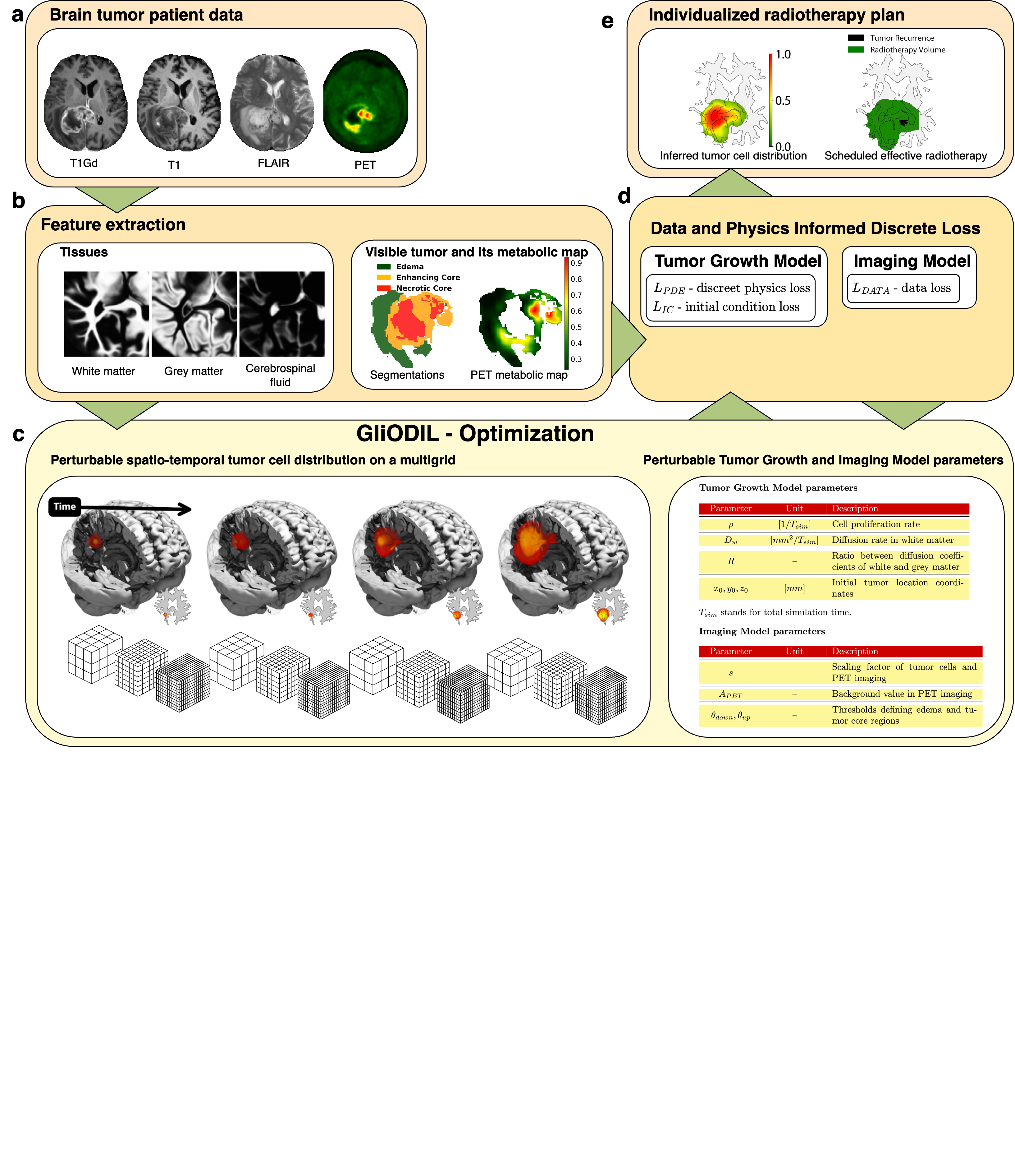
Figure 1: GliODIL overview. a Multi-modal patient data consisting of MR and PET imaging. b To define the input grid conditions and tumor boundaries, tissue extraction (using an atlas registration; left) and automatic brain tumor segmentation (right) is performed. Automatically segmented tumor regions include three components:(i) edema, characterized by tissue swelling due to fluid accumulation; (ii) enhancing core, indicative of active tumor growth and characterized by vascular leakage, and (iii) necrotic core, showing tissue death due to hypoxia or nutrient deprivation. Corresponding PET scans provide metabolic insight, further aiding in accurate tumor delineation. c Spatio-temporal progression of a tumor within patient anatomy. Values are stored on a multi-resolution grid where each level is coarser than the other. Optimization utilizes automatic differentiation and is guided by the loss function. Since we model the progression based on a single time-point input data, the growth parameters are being resolved up to a timescale. d Calculation of discrepancy between patient’s tumor characteristics $L_{\text{DATA}}$ and proposed by GliODIL tumor cell-distribution’s final timestep. Tumor growth physics is encapsulated in a partial differential equation (PDE). Calculation of PDE’s residual $L_{\text{PDE}}$ and single focal initial condition $L_{\text{IC}}$. e GliODIL outputs. The framework successfully infers the complete distribution of tumor cells, facilitating the development of a radiotherapy plan. This plan effectively covers areas of tumor recurrence identified in post-operative data, while maintaining the total radiotherapy volume in line with standard clinical guidelines.

This work introduces Glioma ODIL (GliODIL), a novel optimization framework designed for estimating tumor cell concentrations and migration pathways surrounding visible tumors in MRI and PET scans, as depicted in Figure 1. Our approach uniquely integrates traditional numerical methods with data-driven paradigms, providing a more comprehensive insight into tumor behavior. In addition to its adaptive capabilities. Building upon our previous work and the Optimizing a Discrete Loss (ODIL) technique, GliODIL significantly enhances computational speed compared to traditional PINNs architectures. Diverging from conventional glioma models that solely alter the parameters of presumed PDEs, our method adapts both the parameters and the discretized solutions. Additionally, it quantifies divergence from physical principles as a measure of quality control. GliODIL achieves a level of fidelity in parameter inference comparable to much more costly Bayesian methods and surpasses Bayesian, data-driven, and population-based models in accurately predicting tumor recurrences, thereby contributing to the evolving landscape of personalized treatment strategies in oncology.

2 Results

Our study begins with a synthetic dataset analysis to validate our model’s performance under different tumor scenarios. We focus on both single and multi-focal tumor cases, highlighting our model’s precision and resilience, even with the inclusion of noise in the synthetic data. We then apply our model to real patient data from 18 individuals (see Section 4.6), aiming to evaluate its robustness in tumor growth parameter inference against benchmarks. Lastly, we compare our model’s predictions as a basis for an individualized radiotherapy plan with clinically applied radiation therapy plans and other state-of-the-art modeling methods to gauge its potential clinical utility. We showcase the output of a forward run utilizing a traditional finite difference method solver. This output, derived from parameters inferred by our GliODIL framework, is referred to as the $\text{PDE}_{\text{GliODIL}}$ output, where PDE corresponds to the fact that the output strictly adheres to the Tumor Growth Model’s underlying PDE. To speed up convergence, we employ a personalized initial guess of tumor cell distribution outlined in detail in Section 4.8.

2.1 Synthetic Patient Data - $L_{\text{PDE}}$ importance calibration

Our main modeling assumption is that tumor growth according to a given PDE is controlled by the loss $L_{\text{PDE}}$ and that it starts from a single focal seed point, controlled by the initial condition $L_{\text{IC}}$ loss. Both of these loses are formally introduced in Section 4.1. We want to test the applicability of these assumptions to more complex, real-world scenarios like multi-focal tumors that break the modeling assumptions. We considered relaxing both assumptions to capture such complex scenarios as multi-focal tumors. Easing the constraints imposed by $L_{\text{IC}}$ results in ambiguities that hinder the reliable determination of tumor growth parameters of single focal tumors, an important aspect of our study. Instead, we opted for experimenting with the $L_{\text{PDE}}$ importance governed by a weighing parameter $\lambda_{\text{PDE}}$ in the final loss.

To add an additional layer of realism, we introduce noise into our PET data using a random Markov field and partial volume effects around necrotic regions to study the robustness of our solution to imperfect data acquisitions, a common challenge in clinical application.

We report the results from 50 synthetic patients, half with single focal tumors and the remaining 25 patients with multi-focal tumors. The outcomes of this experiment are illustrated in Figure 2. In Figure 2e we observe that both high $\lambda_{\text{PDE}}$ (strong adherence to the equation) and low $\lambda_{\text{PDE}}$ (overfitting to the data) are sub-optimal for complex tumors and the $\lambda_{\text{PDE}}=1$ used in GliODIL aligns the closest with the ground truth. The decision to set $\lambda_{\text{PDE}}=1$ represents a balanced choice, enabling accurate inference of single focal tumors (see Figure 2a,b,c) while also capturing a significant portion of the multi-focal ground truth, as shown in Figure 2a,e. This setting of $\lambda_{\text{PDE}}=1$ will be consistently applied in our real patient data studies discussed in Section 2.2.

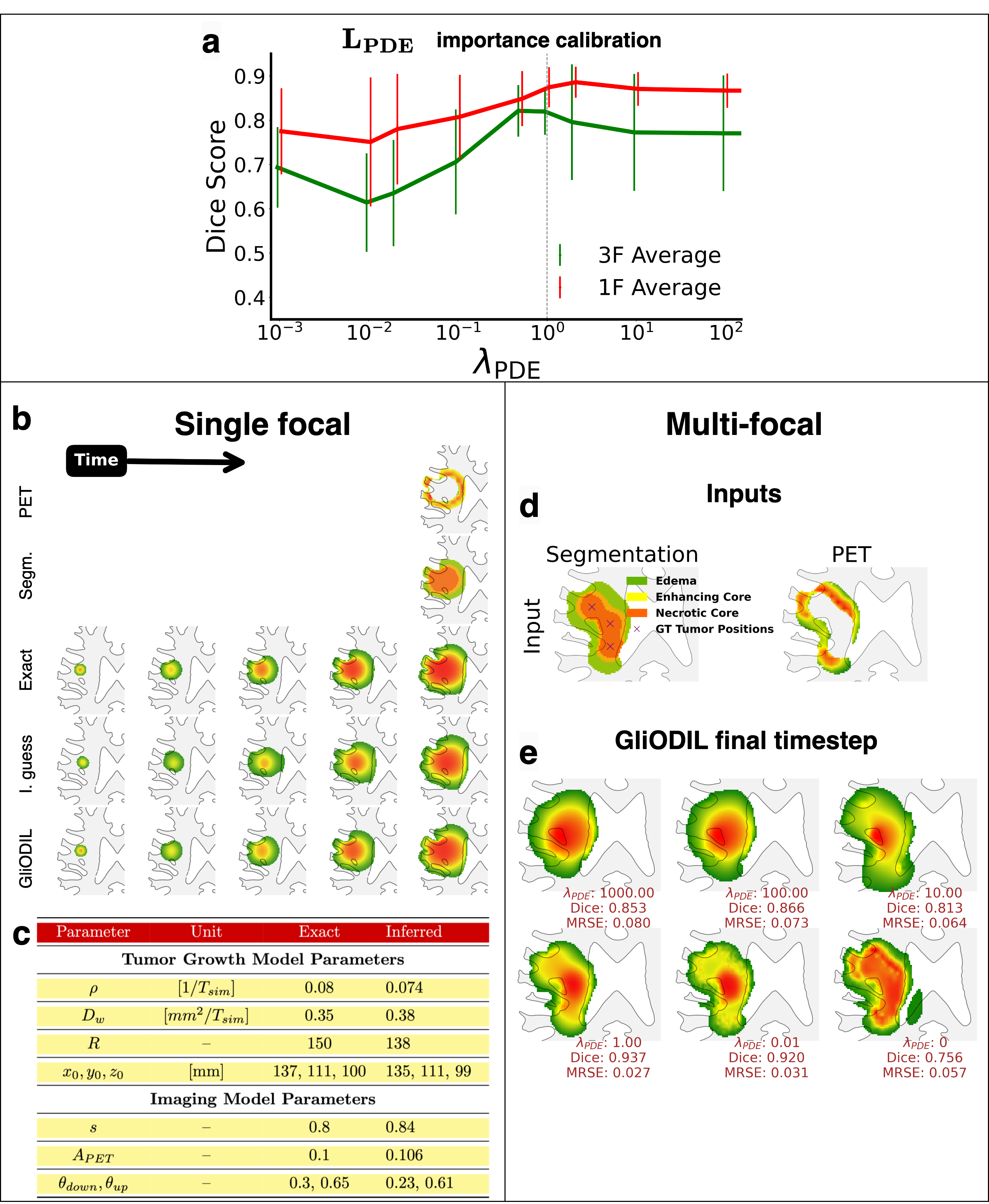
Figure 2: Synthetic dataset experiments overview. a Illustration of GliODIL’s synthetic results for multi-focal (3F) and single focal (1F) tumors. In these simulations, all loss weights remain constant except for the $L_{\text{PDE}}$ weight, $\lambda_{\text{PDE}}$. A value of $\lambda_{\text{PDE}}=1$ was selected to strike a balance in the model. Dice scores were calculated at 10% tumor cell concentration, which is outside of the segmented region (edema at 25%). b Comparison: a forward run with ground truth parameters (Exact), initial guess (I. guess), and a forward PDE run with GliODIL-based inferred parameters ($\text{PDE}_{\text{GliODIL}}$). The first and second columns represent PET and segmentation input to the model to infer the full special-temporal structure. The bottom row shows the input to the pipeline, synthetic PET, and binary MRI segmentations. c Comparison of exact and inferred parameters. d Input for the multi-focal experiment. e Tumor cell distribution of GliODIL with progressively relaxed $\lambda_{\text{PDE}}$. Root Mean Square Error (RMSE) is calculated for low-cell tumor concentration (at 10%), meaning tumor cell distribution far outside of visible tumor on MRI.

2.2 Real Patient Data

We examine the performance of our GliODIL and $\text{PDE}_{\text{GliODIL}}$ outputs on a curated dataset of 18 real patient cases. The analysis is separated into two essential components: parameter inference for the $\text{PDE}_{\text{GliODIL}}$ framework and radiotherapy planning using the GliODIL model directly. We compare our findings against two distinct state-of-the-art approaches for solving the inverse problem in glioma modeling: On the one hand, a Transitional Markov Chain Monte Carlo (TMCMC) implementation [15], a traditional approach, and the Learn-Morph-Infer (LMI) method [22], which is based on a deep learning solution for the tumor growth model parameter inference. For the TMCMC method, we will present only the maximum a posteriori probability (MAP) sample, with further elaboration provided in the discussion section 3. We will refer to TMCMC MAP simply as $\text{PDE}_{\text{MCMC}}$ to highlight the fact that it strictly adheres to the PDE that underlies its tumor growth model. In a similar fashion, we will refer to the output from LMI as $\text{PDE}_{\text{LMI}}$.

2.2.1 Parameter Inference

We visualize two representative cases and present average results with their standard deviations in Figure 3. For a detailed explanation of performance metrics, see Section 4.4. Examining models that strictly adhere to tumor growth models’ PDE, one observes that both $\text{PDE}_{\text{GliODIL}}$ and $\text{PDE}_{\text{MCMC}}$ explain the data at a comparable level, with some trade-offs in specific categories. $\text{PDE}_{\text{GliODIL}}$ shows increased stability, as indicated by reduced variance in its results. In contrast, $\text{PDE}_{\text{LMI}}$, despite its faster inference, performs noticeably worse.

In terms of data explanation, as measured by dice scores and PET signal correlation, GliODIL surpasses all examined PDE solutions. Better fit to the data can be attributed to GliODIL’s ability to balance between adhering to the PDE on which it is being regularized and effectively explaining the data. This performance indicates that its inferred tumor cell distributions could more accurately mirror actual conditions. However, for real patients, unlike in synthetic experiments detailed in Section 2.1, we lack ground truth to directly substantiate these claims and the results might be overfitted through the data-driven term (as in Figure 2e for $\lambda_{\text{PDE}}<1$) . To validate GliODIL’s performance, a downstream task of clinical relevance is performed. In the following Section 2.2.2, we demonstrate that GliODIL leads to more effective radiotherapy plans in terms of tumor recurrence coverage.

The purpose of the parameter inference section is to illustrate that the parameters inferred through $\text{PDE}_{\text{GliODIL}}$ explain the data as effectively or better than traditional, slower methods, and that inferred parameters can be utilized for diagnostics and forecasting.

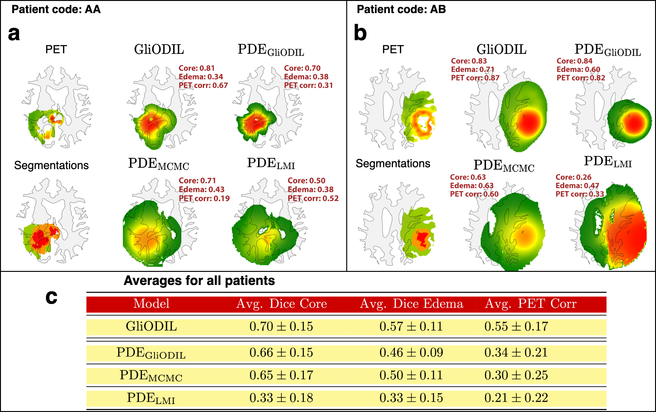
Figure 3: Real patient data. Parameter inference overview. a, b Comparison of tumor cell density predictions from various models with corresponding data inputs. Threshold values for each model are determined through a grid search, since the LMI model does not infer them. c Average scores for each model calculated for all patients.

2.2.2 Radiotherapy planning and recurrence coverage

We develop a framework to compare radiation volumes from clinically applied radiotherapy plans according to the ESTRO guidelines (referred here as the Standard Plan), planned with a uniform 1.5 cm margin surrounding the visible tumor core, with those delineated by thresholding the output of computational tumor models to match the 3D volume of the Standard Plan, i.e., to re-distribute the uniform standard radiotherapy volume to better capture the predicted tumor cell spread. The primary measure for assessing the model’s effectiveness is its precision in forecasting recurrent tumor within the designated radiation volume post-surgery. Although this metric is not the sole indicator of the model’s validity — since it does not consider variables such as the extent of surgical resection and the impact of radiotherapy — it still provides significant insights into the model’s capabilities to serve as the basis for an individualized radiotherapy plan by capturing the tumor cell distribution beyond the visible tumor margins. The residual tumor cells can give rise to a later recurrence, as most glioblastoma recurrences occur near the surgical resection cavity. We define two key metrics of interest: a) Recurrence Coverage [%] and b) Preferred Plan [%] (see Section 4.4 for more details). Recurrence Coverage refers to the percentage of segmented recurrences identified via segmentation of follow-up MRIs showing tumor recurrence according to the current RANO guidelines, which are encompassed within the clinical radiation target volume. The Preferred Plan metric quantifies the percentage of instances in which the method was considered superior recurrence coverage-wise or achieved 100% recurrence coverage, on par with alternative methods. These comparative evaluations are graphically depicted in Figure 4 together with the average outcomes of these measures.

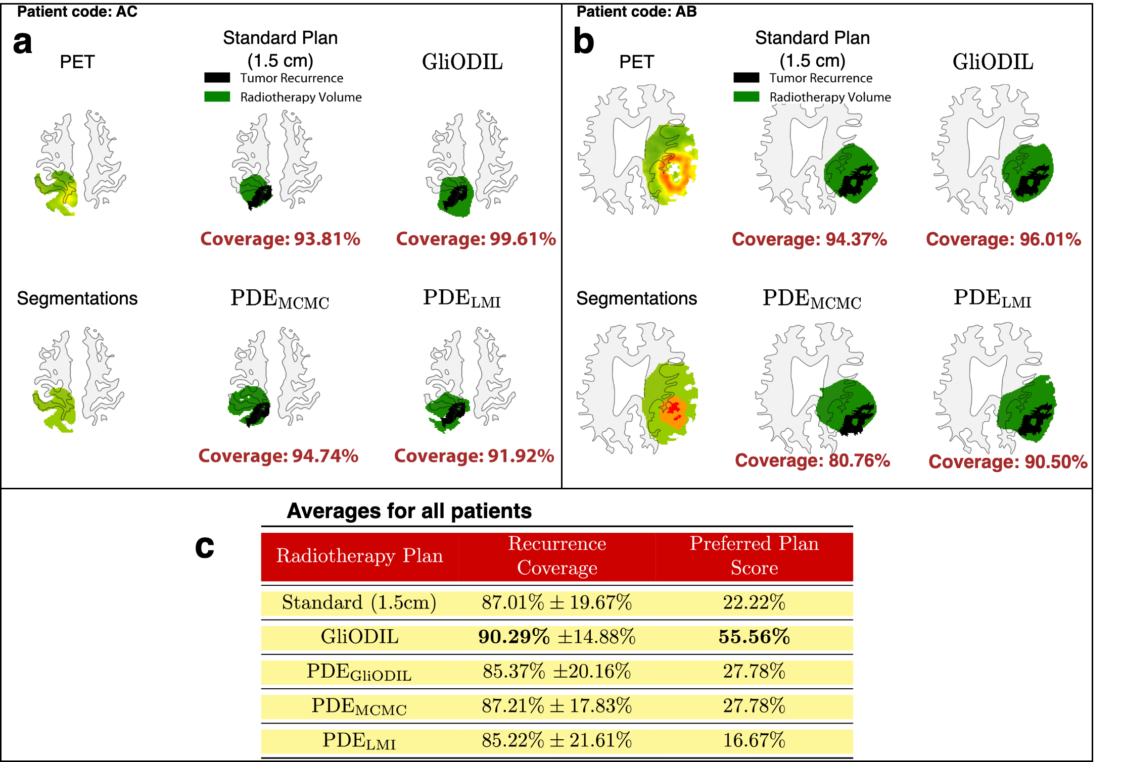
Figure 4: Real patient data. Recurrence coverage overview. a,b Recurrence coverage of selected equal 3D volume radiotherapy plans. Output tumor cell distribution thresholds found through a grid search to match the Standard Plan volumes. c Average Recurrence Coverage and Preferred Plan statistics.

In head-to-head comparisons with the clinically applied radiotherapy protocols, GliODIL consistently yielded superior performance when matching the radiotherapy volume. Established methods for estimating tumor cell distributions by inverting for PDE parameters and running a forward simulation in patient’s anatomy, $\text{PDE}_{\text{MCMC}}$ and $\text{PDE}_{\text{LMI}}$, were inferior to GliODIL. The method also provides lower results variance. Both the Recurrence Coverage and Preferred Plan columns in Figure 4 highlight the superior performance of the GliODIL method. It’s important to note that the high standard deviations in the Recurrence Coverage column is not indicative of the methods unreliability, but rather reflects the inherent complexity of predicting tumor recurrences, which can vary significantly in difficulty from case to case. Despite this natural variance, the averages in the Recurrence Coverage column are a reliable predictor of the effectiveness of each planning method. Although the $\text{PDE}_{\text{GliODIL}}$ output yielded results less effective than those from GliODIL, it affirmed the benefit of relaxing the strict PDE constraints typically employed in forward runs. Relaxing the PDE constraint proved to be advantageous for designing radiotherapy plans, where the objective is to identify probable tumor locations. Achieving this requires a nuanced balance between the significance of data and the tumor growth equations. To facilitate a comparison between $\text{PDE}_{\text{GliODIL}}$, which strictly adheres to the tumor growth PDE, and GliODIL, we present Figure 5. The figure illustrates that while $\text{PDE}_{\text{GliODIL}}$ may perform on par or better than the benchmarks discussed in Section 2.2 in terms of explaining patient data, it struggles to accurately represent complex tumor cases where the PDE is far from describing reality. This limitation leads to the omission of certain tumor recurrences. In contrast, GliODIL adapts to potential discrepancies in the equations by incorporating additional tumor cells around areas of high PET signal and the enhancing core through the data-driven part, thereby enhancing the rate of recurrence coverage.

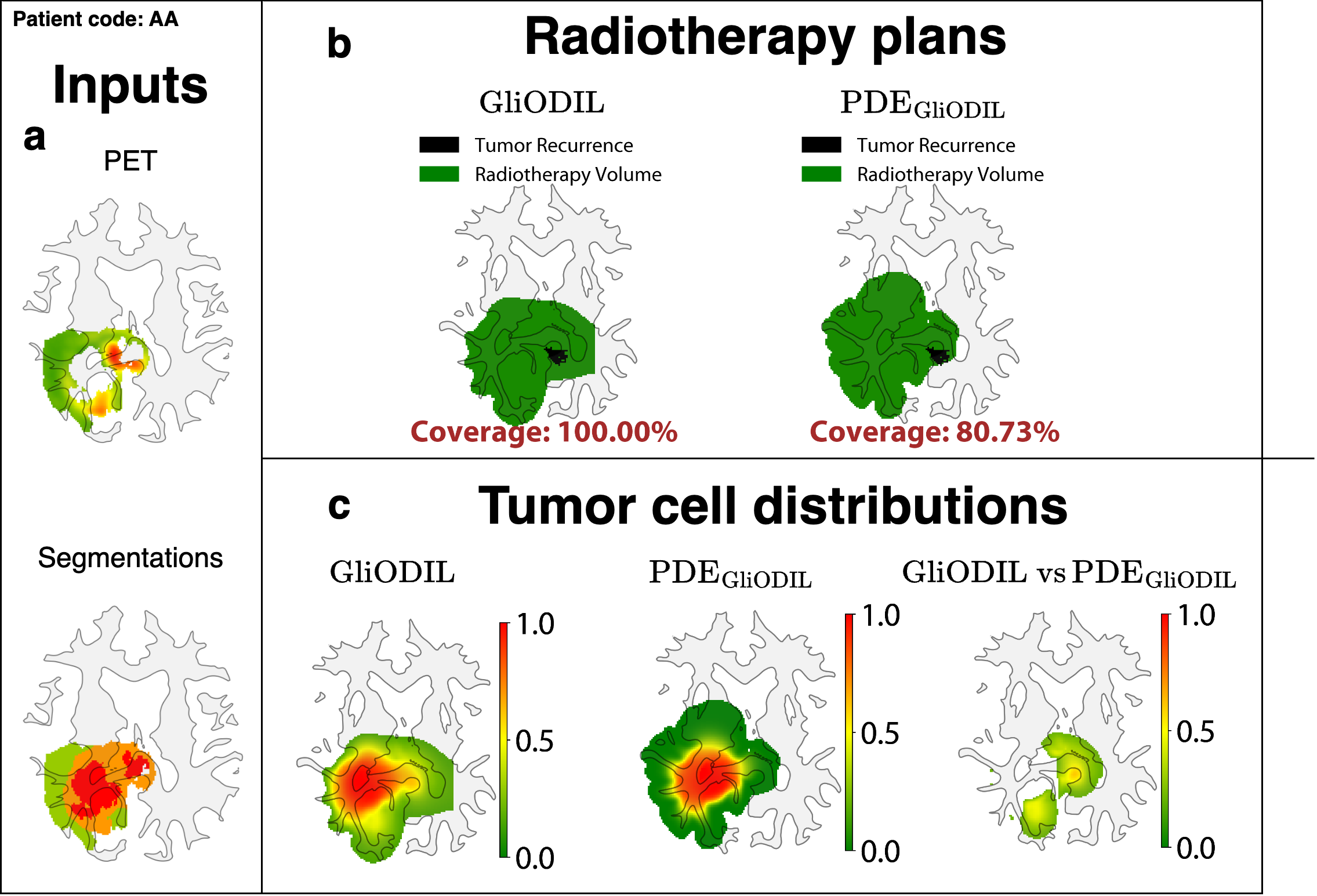
Figure 5: Comparison between GliODIL and $\text{PDE}_{\text{GliODIL}}$ a Inputs to the model: PET metabolic map and tumor segmentations. b Radiotherapy plans for GliODIL and $\text{PDE}_{\text{GliODIL}}$. Both plans have equal radiation volumes to the Standard Plan (1.5cm around the tumor core segmentation). c Tumor cell distributions for GliODIL, $\text{PDE}_{\text{GliODIL}}$ within their radiotherapy regions. In addition, absolute difference between GliODIL and $\text{PDE}_{\text{GliODIL}}$ distributions plotted above 20%.

3 Discussion

In this work, we have introduced GliODIL, a framework that adeptly balances the fidelity of tumor growth model parameters with the computational demands of more extensive methods. This balance is achieved through a novel joint data- and physics-constrained formulation, utilizing multi-grid domain and automatic differentiation to model reaction-diffusion brain tumor growth. Our findings demonstrate the potential of GliODIL in predicting the full spatial distributions of tumor cells, showing promising results in recurrence coverage that surpass other studied methods. This success suggests that easing the constraints of the Tumor Growth Model can enhance the accuracy of tumor recurrence forecasts by aligning more closely with empirical data while still weakly adhering to theoretical models and having quality control measures. With the availability of time-series data, we are presented with the intriguing possibility of not only relaxing the Tumor Growth Model but also potentially refining the single focal initial condition constraints. This approach could be pursued without significantly increasing the ill-posedness of the system, representing a promising direction for future research.

For benchmarking purposes, even though the computational expenses of MCMC restrict its practical use in clinical settings, it presents an intriguing comparison opportunity by generating an ensemble of tumor simulations and merging them into a single tumor cell distribution. These would be sampled from the inferred posterior distribution, allowing for a range of possible parameter scenarios. The method would not strictly conform to a single Tumor Growth Model like the MCMC’s maximum a posteriori probability sample used in this study ($\text{PDE}_{\text{MCMC}}$) but would still operate under a degree of quality control, offering a nuanced approach to model evaluation.

We are interested in extending our GliODIL framework to incorporate mass effects through dynamic tissue models and adopting a Lagrangian frame of reference, rather than solving for dynamical tissues in a static Eulerian frame.

Multimixture models present an attractive alternative, particularly in eliminating issues related to the partial volume effect. In addition to reaction-diffusion processes, we consider modeling narrow interfaces between different tumor cells, which adds another layer of complexity in terms of computational domain remeshing. On the methodological side, addressing uncertainties in parameter inference remains a crucial focus. This could be achieved by integrating variational inference techniques into the framework. In future works,

As we continue to explore and refine GliODIL, our goal is to contribute to the broader understanding of tumor dynamics and to support the development of personalized treatment strategies in oncology. In addition, we are confident that our approach, which employs PDEs and initial conditions as a form of regularization rather than strict constraints, and our strategy of relaxing these elements to encompass more complex dynamics, can be effectively applied to other inverse problems in biology. GliODIL method, favoring adaptability over the use of overly sophisticated models with limited data and computational constraints, holds potential for broader applications.

4 Methods

4.1 Tumor Growth Model

The core of our forward model rests on the Fisher-Kolmogorov Reaction-Diffusion (FK) equation, tailored for simulating tumor growth dynamics in terms of cellular diffusion and proliferation.

The partial differential equation (PDE) characterizing this model delineates the spatio-temporal evolution of the normalized tumor cell density $u(x,y,z,t)$ across a three-dimensional patient-specific brain anatomy segmented from MRI scans. The governing equation is:

$$\frac{\partial u(x,y,z,t)}{\partial t} =\nabla\cdot(D\nabla u)+\rho u(1-u)$$ (1)

The proliferation rate of the tumor is denoted by $\rho$, while $D(x,y,z)$ serves as the spatially varying diffusion coefficient that captures the tumor’s invasive characteristics. In the simulation, we enforce a no-flux boundary condition at the edges of the computational domain, confined to brain tissue.

We impose an initial condition in accordance with Equation 1 as follows:

$$u(x,y,z,0) =G(x,y,z)$$ (2)

where for $G(x,y,z)$ we employ a Gaussian function centered at an origin point $\mathbf{r}_{0}$, as shown in Equation 3:

$$\small G(\mathbf{r}) =C_{1}\exp\left(-\frac{(\mathbf{r}-\mathbf{r}_{0})^{2}}{C_{2}}\right)$$ (3)

where we set the constants to $C_{1}=\frac{50}{(60\pi)^{3/2}}$, $C_{2}=60$, which correspond to the initial tumor sizes depicted in Figure 1 and Figure 2.

For further definitions we assume discretization of the domain for computational purposes. Each voxel at coordinates $(i_{x},i_{y},i_{z})$ is attributed a diffusion coefficient $D_{i,j,k}$, calculated as:

$$D_{i,j,k}=w_{i,j,k}D_{w}+g_{i,j,k}D_{g}$$ (4)

Here, $w_{i,j,k}$ and $g_{i,j,k}$ signify the proportions of white matter (WM) and gray matter (GM) at voxel $(i_{x},i_{y},i_{z})$, respectively. $D_{w}$ and $D_{g}$ represent the diffusion coefficients associated with WM and GM. We make the assumption $D_{w}=R\cdot D_{g}$, with $R>1$ being an unknown constant.

The residuals from Equations 1 and 2 are utilized to construct the loss function components $L_{\text{PDE}}$ and $L_{\text{IC}}$, respectively. These components are meant to quantify the divergence of the proposed tumor cell density $u(x,y,z,t)$ from the outcomes of the FK model. The process of discretizing $L_{\text{IC}}$ is straightforward, while the discretization approach for $L_{\text{PDE}}$ is delineated in Section 4.2.

In this configuration, both the tumor’s origin point $\mathbf{r}_{0}=(x_{0},y_{0},z_{0})$ and the parameters associated with tumor dynamics $D,\rho,R$ are treated as unknowns that needs to be inferred.

4.2 Optimizing a Discrete Loss (ODIL)

ODIL is a framework that addresses the challenges of solving inverse problems. It works by discretizing the PDE of the forward problem and using machine learning tools like automatic differentiation and popular deep learning optimizers (ADAM/L-BFGS) to minimize its residual while maintaining its sparse structure.

The previously introduced FK PDEs are discretized to perform numerical computations. We define $\Omega_{1}$ as the region within the brain where tumor cells can diffuse, primarily within the gray and white matter. Let’s introduce the diffusion term $A$ and the reaction term $B$:

$$A(u_{i,j,k}^{n}) =\frac{1}{\Delta x^{2}}\left(D_{i+\frac{1}{2},j,k}(u_{i+1,j,k}^{n}-u_{i,j,k}^{n})-D_{i-\frac{1}{2},j,k}(u_{i,j,k}^{n}-u_{i-1,j,k}^{n})\right)$$

$$+\frac{1}{\Delta y^{2}}\left(D_{i,j+\frac{1}{2},k}(u_{i,j+1,k}^{n}-u_{i,j,k}^{n})-D_{i,j-\frac{1}{2},k}(u_{i,j,k}^{n}-u_{i,j-1,k}^{n})\right)$$

$$+\frac{1}{\Delta z^{2}}\left(D_{i,j,k+\frac{1}{2}}(u_{i,j,k+1}^{n}-u_{i,j,k}^{n})-D_{i,j,k-\frac{1}{2}}(u_{i,j,k}^{n}-u_{i,j,k-1}^{n})\right)$$ (5)

$$B(u_{i,j,k}^{n})=\rho u_{i,j,k}^{n}(1-u_{i,j,k}^{n})$$ (6)

Utilizing the Crank-Nicolson scheme, the residual PDE loss can be expressed as:

$$R_{i,j,k}^{n}=\frac{u_{i,j,k}^{n+1}-u_{i,j,k}^{n}}{\Delta t}-\frac{A(u_{i,j,k}^{n+1})+A(u_{i,j,k}^{n})}{2}-\frac{B(u_{i,j,k}^{n+1})+B(u_{i,j,k}^{n})}{2}$$ (7)

$$L_{\text{PDE}}(u,D_{w},\rho,R)=\sum_{(i,j,k,n)\in\Omega_{1}}(R_{i,j,k}^{n})^{2}$$ (8)

Boundary conditions, particularly no-flux conditions outside $\Omega_{1}$, are employed to provide an accurate description of tumor cell behavior. The diffusion coefficients between gridpoints and within the tissue region $\Omega_{1}$ are computed as the average of their neighboring values.

The multi-grid ODIL technique, introduced in the paper [24], builds upon the original ODIL methodology by incorporating a multigrid decomposition scheme to hasten the convergence process. This technique is particularly adept at leveraging the multi-scale attributes of the forward problem. It decomposes the problem into various scale bands, each characterized by different levels of detail. Formally, for a uniform grid with dimensions $N_{1}=N$, a hierarchical sequence of coarser grids is introduced with sizes defined as $N_{i}=N/2^{i-1}$ for $i=1,\ldots,L$.

$$M_{L}(u_{1},\ldots,u_{L})=u_{1}+T_{1}u_{2}+T_{1}T_{2}\ldots T_{L-1}u_{L},$$ (9)

where each $u_{i}$ is a field on grid $N_{i}$, and $T_{i}$ serves as an interpolation operator mapping from coarser grid $N_{i+1}$ to its finer counterpart $N_{i}$. The discrete field $u$ on an $N$-sized grid is thus decomposed as $u=M_{L}(u_{1},\ldots,u_{L})$.

As depicted in Figure 1c, which illustrates the multigrid domain, a tumor growth is simulated over an ensemble of Cartesian 4D grids in both time and space, with each grid level being coarser than the preceding one. This hierarchical decomposition allows the optimization algorithm to initially concentrate on the coarse-scale features, incrementally incorporating finer-scale details as the process evolves. Such an approach not only enables a more comprehensive exploration of the parameter space but also sidesteps the pitfalls of local minima and expedites convergence.

4.3 Imaging Model

The imaging model we present serves as a bridge between the simulated tumor cell densities and the imaging signatures captured in MRI and PET scans. This model translates tumor cell density, denoted as $u$, into quantifiable imaging signals that reflect observed clinical phenomena and imaging physics principles.

The core of the model’s data-driven nature is encapsulated by the loss function $L_{\text{DATA}}$, which associates the simulated outputs with key imaging traits such as the tumor core, surrounding edema, and metabolic activity detected through PET imaging. This loss function integrates four adjustable parameters $\{\theta_{\text{down}},\theta_{\text{up}},s,A_{\text{PET}}\}$ and is expressed as:

$$L_{\text{DATA}}=\lambda_{\text{CORE}}L_{\text{CORE}}(u,\theta_{\text{up}})+\lambda_{\text{EDEMA}}L_{\text{EDEMA}}(u,\theta_{\text{down}},\theta_{\text{up}})+\lambda_{\text{PET}}L_{\text{PET}}(u,s,A_{\text{PET}})$$ (10)

where $\lambda_{\text{CORE}},\lambda_{\text{EDEMA}},\lambda_{\text{PET}}$ are weights. The loss function is composed of individual terms corresponding to distinct anatomical features:

• $L_{\text{CORE}}$ relates tumor cell concentrations above the threshold $\theta_{\text{up}}$ to the tumor core region

• $L_{\text{EDEMA}}$ delineates the edema area surrounding the tumor, regulated by the lower and upper thresholds $\theta_{\text{down}}$ and $\theta_{\text{up}}$.

• $L_{\text{PET}}$ reflects the metabolic activity as indicated by PET signals, influenced by a scaling factor $s$ and an offset $A_{\text{PET}}$.

These adaptive parameters $\{\theta_{\text{down}},\theta_{\text{up}},s,A_{\text{PET}}\}$ enable the model to accommodate variations in MRI/PET imaging contrasts and noise levels.

We adopt sigmoid functions to portray the gradational transitions observed at tumor region margins. The sigmoid, $\sigma(x)$, is specified as:

$$\sigma(x)=\frac{1}{1+e^{-\beta x}}$$ (11)

Here, $\beta$ modulates the steepness of the transition and is set to $\beta=50$. For the tumor core:

$$L_{\text{CORE}}(u,\theta_{\text{up}})=\sum_{(i,j,k,n)\in\Omega_{2}}\sigma(\theta_{\text{up}}-u^{n}_{i,j,k}-\alpha)$$ (12)

for the edema:

$$L_{\text{EDEMA}}(u,\theta_{\text{down}},\theta_{\text{up}})=\sum_{(i,j,k,n)\in\Omega_{2}}\sigma(\theta_{\text{down}}-u^{n}_{i,j,k}-\alpha)+(1-\sigma(\theta_{\text{up}}-u^{n}_{i,j,k}+\alpha))$$ (13)

where $\alpha$ offsets the thresholds and is set to $\alpha=0.05$.

In this context, $\Omega_{2}$ represents the collection of voxels that map to the time point at which the imaging is conducted; for single-image analysis, this corresponds to the final time slice. See Figure 6 for the shape of segmentation penalty function.

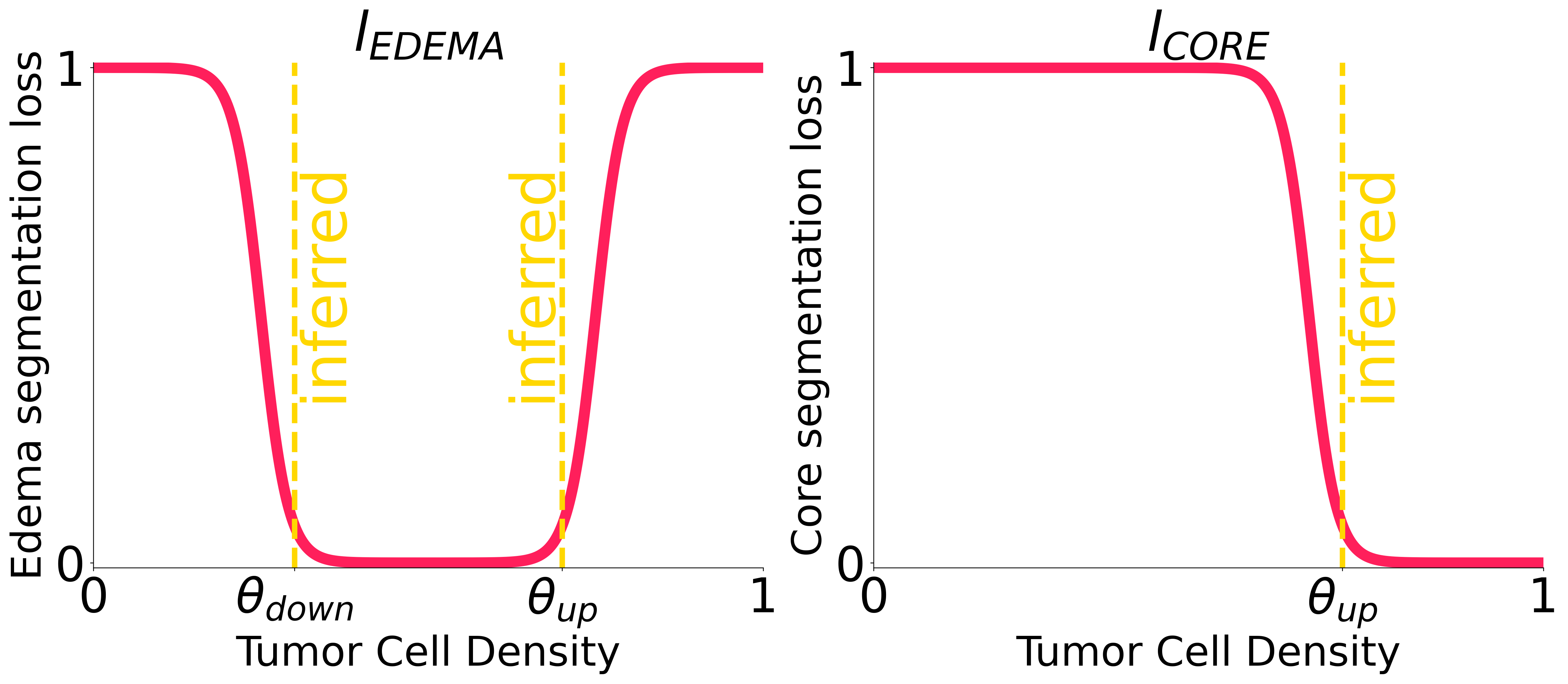
Figure 6: Visualization of the segmentation penalty function with adaptive thresholds $\theta_{\text{down}}$ and $\theta_{\text{up}}$. These thresholds are determined during the optimization process to adapt to the unique characteristics and sensitivities of different MRI images and tumor types.

The metabolic activity within the tumor is evaluated by the loss term $L_{\text{PET}}$, which aligns the simulated metabolic signal with actual PET scan observations:

$$L_{\text{PET}}(u,s,A_{\text{PET}})=\sum_{(i,j,k,n)\in\Omega_{3}}(u^{n}_{i,j,k}-p^{\text{PET}}_{i,j,k})^{2}$$ (14)

For this purpose, $\Omega_{3}$ is defined as the subset of $\Omega_{2}$ where voxels are attributed to the metabolically active regions, specifically the enhancing tumor core and the edema, as visualized in Figure 1 in the feature extraction. Regions manifesting necrosis are omitted due to their lack of metabolic activity, and areas beyond the edema and enhancing core are also excluded to minimize noise interference, which is assumed to offer negligible informative value.

Here $p^{\text{PET}}_{i,j,k}$ is the normalised to $[0,1]$ PET signal $y_{i,j,k}^{\text{PET}}$ scaled by $s$ and with an offset $A_{\text{PET}}$:

$$p^{\text{PET}}_{i,j,k}=s\cdot y_{i,j,k}^{\text{PET}}+A_{\text{PET}}$$ (15)

The devised loss function $L_{\text{DATA}}$ quantifies the discrepancies between simulated tumor cell densities and empirical imaging data.

4.4 Evaluation Metrics

We introduce specific metrics to evaluate the performance of the proposed GliODIL framework. These metrics include the Dice score, PET signal correlation, Recurrence Coverage, and the Preferred Plan metric.

Dice score

The Dice score, also known as the Sørensen–Dice index or Dice coefficient, is a widely recognized metric in medical image analysis for quantifying the similarity between two volumes. The coefficient is defined as twice the area of overlap between the two volumes divided by the total number of voxels in both samples:

$$\text{Dice Coefficient}=\frac{2\times|A\cap B|}{|A|+|B|}$$ (16)

where $A$ represents the thresholded tumor volume from a computational model and $B$ represents the segmented tumor volume from patient MRI segmentations or thresholded ground truth tumor volume. This index ranges from 0 to 1, where 0 indicates no overlap and 1 indicates perfect agreement between the two segmented regions.

PET Signal Correlation

This metric calculates the Pearson’s correlation coefficient between PET signal intensity and tumor cell concentration in regions where a high degree of correlation is expected: the enhancing core and the edema.

Recurrence Coverage and Preferred Plan

The primary measure for assessing the model’s radiotherapy effectiveness is its precision in forecasting recurrent tumor within the designated radiation volume post-treatment. Tumor recurrence area we define as segmented enhancing and necrotic tumor core in post-treatment patient data. We register the post-treatment patient anatomy to the pre-treatment in order to remove special shifts due to surgeries. Two key metrics of interest in this context are:

• Recurrence Coverage [%]: This metric refers to the percentage of segmented recurrences, identified via segmentation of follow-up MRIs, that are encompassed within the radiation volume delineated by our model.

• Preferred Plan [%]: This metric quantifies the percentage of instances in which a given method was considered superior recurrence coverage-wise compared to all other methods or achieved 100% recurrence coverage tied with another method.

4.5 Preprocessing of Input Data

We preprocess MRI and PET images using BraTS Toolkit [25] resulting in images resolution of $240\times 240\times 155$ with segmented tumor regions. Given our assumption that surrounding tissues remain static, we segment brain tissues based on atlas registration [15] and focus the computational grid specifically on the tumor region. This leads to an average resolution of $71\times 68\times 55$ for the area of interest in our images. For parameter inference within the GliODIL framework, we employed a $48^{3}$ spacial resolution and 192 degrees in the temporal resolution. Our tests indicated that this resolution is sufficient, revealing no significant differences compared to inference using the native resolution. For a forward PDE run with inferred parameters by GliODIL, which we call $\text{PDE}_{\text{GliODIL}}$, we use the native resolution.

In the creation of synthetic PET images, we implement a sequence of processing steps to emulate real-world PET imaging characteristics. Initially, we introduce spatially correlated noise using the Gibbs method to simulate the inherent noise in PET scans. Following this, we remove the necrotic core area from the images, reflecting the typical absence of metabolic activity in these regions in actual PET scans. Subsequently, we apply a downsampling process by a factor of 4, followed by an upsampling using zeroth-order spline interpolation. This sequence of downscaling and upscaling to an effective low resolution of 4mm is designed to simulate the lower resolution and partial volume effects commonly observed in real PET images.

4.6 Datasets

For loss function weights calibration purposes, we created the synthetic dataset for single focal tumor and multi-focal by solving the system of differential equations using a traditional FDM solver. In this case, for the tissue distribution we use an atlas brain. We variate ground truth tumor growth model parameters, imaging model parameters and focal locations using a uniform random distribution. In addition to the parameters outlined in Table 1, here we introduce an extra threshold, $\theta_{\text{necro}}$, above which the region is treated as a necrotic core without PET metabolic activity. The range of parameters utilized in the generation is summarized in Table 1.

For the analysis of real patient data, we chose 10 patients at random from our database at Klinikum Rechts Der Isar. Additionally, we included 8 patients from the study conducted by Lipkova et al. (2019) [15].

Shared Parameters
Parameter	Min	Max
$D_{w}$	0.035	0.2
$\rho$	0.035	0.2
$R$	10	30
$\theta_{\text{necro}}$	0.70	0.85
$\theta_{\text{up}}$	0.45	0.60
$\theta_{\text{down}}$	0.15	0.35
$T_{\text{sim}}$	100
Single Focal Tumor Center (mm)
($x$, $y$, $z$)	57.6	96
Multi-Focal Tumor Centers (mm)
Tumor 1 Center ($x$, $y$, $z$)	57.6	96
Tumor 2 Center ($x_{2}$, $y_{2}$, $z_{2}$)	($x_{1}$, $y_{1}$, $z_{1}$) $\pm$ 9.6
Tumor 2 Center ($x_{3}$, $y_{3}$, $z_{3}$)	($x_{2}$, $y_{2}$, $z_{2}$) $\pm$ 9.6

Table 1: Parameter Ranges for Generating Synthetic Single Focal and Multi-Focal Tumor Datasets

4.7 Final Loss Function

The final loss function measures discrepancy between proposed tumor cell concentrations $u(x,y,z,t)$ and our objective. It is a composite term that comprises contributions from multiple sources: the PDE constraint, data fitting, and additional regularization term. Specifically, the PDE loss, denoted by $L_{\text{PDE}}$ (introduced in 4.2), imposes the discretized PDE equation constraint. Initial condition loss term $L_{\text{IC}}$ in the overall loss function serves to enforce that the tumor at $t=0$ originates from a Gaussian origin (introduced in 4.1). The data loss (introduced in 4.3), denoted by $L_{\text{DATA}}=\lambda_{\text{CORE}}L_{\text{CORE}}+\lambda_{\text{EDEMA}}L_{\text{EDEMA}}+\lambda_{\text{PET}}L_{\text{PET}}$, accounts for matching tumor core and edema segmentations as well as fitting to PET metabolic data. Additional regularization term confines the inferred parameters within a plausible range $L_{\text{PARAMS}}$[26].

The overall loss function can thus be expressed as:

$$\mathcal{L}=\; \lambda_{\text{PDE}}L_{\text{PDE}}+\lambda_{\text{IC}}L_{\text{IC}}+\lambda_{\text{CORE}}L_{\text{CORE}}$$ (17)

$$+\lambda_{\text{EDEMA}}L_{\text{EDEMA}}+\lambda_{\text{PET}}L_{\text{PET}}+\lambda_{\text{PARAMS}}L_{\text{PARAMS}}$$ (18)

where $\lambda_{*}$ are weights that will be chosen in Section 2.1 experiments.

4.8 Initial Guess

We aim to solve the optimization problem for the model parameters referenced in a table in Figure 1 as well the tumor concentration field $u(x,y,z,t)$ on a 4D discrete grid. A meaningful initial guess for these values is crucial for the time of the optimization process and the overall success. Initial tumor location coordinates $x_{0},y_{0},z_{0}$ we assume to be in the center of the tumor core. For the guess we assume $\{R,s,A_{\text{PET}},\theta_{\text{down}},\theta_{\text{up}}\}$ to be in the middle of the plausible range[27]. Here, we describe the procedure followed to obtain the remaining $\{u,D,\rho\}$:

1. Initiate a forward run propagation using characteristic values: $D_{\text{ch}}=\frac{V_{\text{EDEMA}}}{V_{\text{CORE}}}$, $\rho_{\text{ch}}=1$. Here, $V_{\text{EDEMA}}$ and $V_{\text{CORE}}$ refer to the volumes of the edema and tumor core segmentations, respectively. Concurrently, track the Dice coefficients for both the tumor core and edema.

2. Terminate the forward run when a local maximum is reached for the segmentation volume-weighted sum of the Dice scores. Document the time at this instance as $T_{\text{ch}}$ and the tumor cell concentration as $u_{\text{ch}}$.

3. For the initial guess, we use $u=u_{\text{ch}}$ as the tumor cell concentration and $D=\frac{D_{\text{ch}}}{T_{\text{ch}}}$, $\rho=\frac{\rho_{\text{ch}}}{T_{\text{ch}}}$ as the initial dynamics.

For a comparative analysis between the initial guess and the $\text{PDE}_{\text{GliODIL}}$ results, see Figure 2.

4.9 Time Complexity

We summarize the execution times of all methods used in the experiments in Table 2.

Model	Evaluation Time
$\text{PDE}_{\text{MCMC}}$	1 day
GliODIL/$\text{PDE}_{\text{GliODIL}}$	30/33 minutes
$\text{PDE}_{\text{LMI}}$	5 minutes

Table 2: Comparison of model evaluation times. GliODIL, $\text{PDE}_{\text{GliODIL}}$, and $\text{PDE}_{\text{LMI}}$ evaluations were performed on a single GPU, whereas $\text{PDE}_{\text{MCMC}}$ runs on a supercomputer with many hundreds of CPU cores.

5 Data and Code Availability

The synthetic data generated for this study, along with the real patient data utilized, are both available for reproduction and benchmarking using the resources provided at github.com/m1balcerak/GliODIL/.

6 Acknowledgment

We would like to extend our gratitude to Bastian Wittmann from the University of Zurich and Tobias Duswald from the Technical Universtity of Munich for their assistance with the manuscript.

References

- \bibcommenthead
- van den Bent et al. [2023] Bent, M.J., Geurts, M., French, P.J., Smits, M., Capper, D., Bromberg, J.E.C., Chang, S.M.: Primary brain tumours in adults. Lancet (2023) https://doi.org/10.1016/S0140-6736(23)01054-1
- Ostrom et al. [2023] Ostrom, Q.T., Price, M., Neff, C., Cioffi, G., Waite, K.A., Kruchko, C., Barnholtz-Sloan, J.S.: Cbtrus statistical report: Primary brain and other central nervous system tumors diagnosed in the united states in 2016-2020. Neuro Oncol (2023) https://doi.org/10.1093/neuonc/noad149
- Louis et al. [2021] Louis, D.N., Perry, A., Wesseling, P., Brat, D.J., Cree, I.A., Figarella-Branger, D., Hawkins, C., Ng, H.K., Pfister, S.M., Reifenberger, G., Soffietti, R., Deimling, A., Ellison, D.W.: The 2021 who classification of tumors of the central nervous system: a summary. Neuro Oncol (2021) https://doi.org/10.1093/neuonc/noab106
- Weller [2021] Weller, M.: Eano guidelines on the diagnosis and treatment of diffuse gliomas of adulthood. Nature Reviews Clinical Oncology 18, 170–186 (2021)
- Niyazi et al. [2023] Niyazi, M., Andratschke, N., Bendszus, M., Chalmers, A.J., Erridge, S.C., Galldiks, N., et al.: Estro-eano guideline on target delineation and radiotherapy details for glioblastoma. Radiother Oncol (2023)
- Frosina [2023] Frosina, G.: Radiotherapy of high-grade gliomas: dealing with a stalemate. Crit Rev Oncol Hematol 190, 104110 (2023) https://doi.org/10.1016/j.critrevonc.2023.104110
- Cristini and Lowengrub [2010] Cristini, V., Lowengrub, J.: Multiscale Modeling of Cancer: An Integrated Experimental and Mathematical Modeling Approach, 1st edn. Cambridge University Press, Cambridge (2010)
- Mang et al. [2020] Mang, A., Bakas, S., Subramanian, S., Davatzikos, C., Biros, G.: Integrated biophysical modeling and image analysis: application to neuro-oncology. Annual review of biomedical engineering 22, 309 (2020)
- Hogea et al. [2008] Hogea, C., Davatzikos, C., Biros, G.: An image-driven parameter estimation problem for a reaction–diffusion glioma growth model with mass effects. Journal of mathematical biology 56(6), 793–825 (2008)
- Lê et al. [2015] Lê, M., Delingette, H., Kalpathy-Cramer, J., Gerstner, E.R., Batchelor, T., Unkelbach, J., Ayache, N.: Bayesian personalization of brain tumor growth model. In: International Conference on Medical Image Computing and Computer-Assisted Intervention, pp. 424–432 (2015). Springer
- Knopoff et al. [2017] Knopoff, D., Fernández, D., Torres, G., Turner, C.: A mathematical method for parameter estimation in a tumor growth model. Computational and Applied Mathematics 36(1), 733–748 (2017)
- Subramanian et al. [2019] Subramanian, S., Gholami, A., Biros, G.: Simulation of glioblastoma growth using a 3d multispecies tumor model with mass effect. J Math Biol 79(3), 941–967 (2019) https://doi.org/10.1007/s00285-019-01383-y
- Scheufele et al. [2020] Scheufele, K., Subramanian, S., Mang, A., Biros, G., Mehl, M.: Image-driven biophysical tumor growth model calibration. SIAM journal on scientific computing: a publication of the Society for Industrial and Applied Mathematics 42(3), 549 (2020)
- Subramanian and et al [2020] Subramanian, S., al: Where did the tumor start? an inverse solver with sparse localization for tumor growth models. Inverse Problems 36(045006) (2020) https://doi.org/10.1088/1361-6420/ab649c
- Lipková et al. [2019] Lipková, J., Angelikopoulos, P., Wu, S., Alberts, E., Wiestler, B., Diehl, C., Preibisch, C., Pyka, T., Combs, S.E., Hadjidoukas, P., et al.: Personalized radiotherapy design for glioblastoma: Integrating mathematical tumor models, multimodal scans, and bayesian inference. IEEE transactions on medical imaging 38(8), 1875–1884 (2019)
- Petersen et al. [2019] Petersen, J., Jäger, P.F., Isensee, F., Kohl, S.A., Neuberger, U., Wick, W., Debus, J., Heiland, S., Bendszus, M., Kickingereder, P., et al.: Deep probabilistic modeling of glioma growth. In: Medical Image Computing and Computer Assisted Intervention–MICCAI 2019: 22nd International Conference, Shenzhen, China, October 13–17, 2019, Proceedings, Part II 22, pp. 806–814 (2019). Springer
- Petersen et al. [2021] Petersen, J., Isensee, F., Köhler, G., Jäger, P.F., Zimmerer, D., Neuberger, U., Wick, W., Debus, J., Heiland, S., Bendszus, M., et al.: Continuous-time deep glioma growth models. In: Medical Image Computing and Computer Assisted Intervention–MICCAI 2021: 24th International Conference, Strasbourg, France, September 27–October 1, 2021, Proceedings, Part III 24, pp. 83–92 (2021). Springer
- Mascheroni et al. [2021] Mascheroni, P., Savvopoulos, S., Alfonso, J.C.L., Meyer-Hermann, M., Hatzikirou, H.: Improving personalized tumor growth predictions using a bayesian combination of mechanistic modeling and machine learning. Communications medicine 1(1), 19 (2021)
- Wang et al. [2022] Wang, H., Argenziano, M.G., Yoon, H., Boyett, D., Save, A., Petridis, P., Savage, W., Jackson, P., Hawkins-Daarud, A., Tran, N., et al.: Biologically-informed deep neural networks provide quantitative assessment of intratumoral heterogeneity in post-treatment glioblastoma. bioRxiv, 2022–12 (2022)
- Nardini et al. [2020] Nardini, J.T., Lagergren, J.H., Hawkins-Daarud, A., Curtin, L., Morris, B., Rutter, E.M., Swanson, K.R., Flores, K.B.: Learning equations from biological data with limited time samples. Bulletin of mathematical biology 82, 1–33 (2020)
- Ezhov et al. [2021] Ezhov, I., Mot, T., Shit, S., Lipkova, J., Paetzold, J.C., Kofler, F., Pellegrini, C., Kollovieh, M., Navarro, F., Li, H., et al.: Geometry-aware neural solver for fast bayesian calibration of brain tumor models. IEEE Transactions on Medical Imaging 41(5), 1269–1278 (2021)
- Ezhov et al. [2022] Ezhov, I., Scibilia, K., Franitza, K., Steinbauer, F., Shit, S., Zimmer, L., Lipkova, J., Kofler, F., Paetzold, J., Canalini, L., Waldmannstetter, D., Menten, M.J., Metz, M., Wiestler, B., Menze, B.: Learn-morph-infer: a new way of solving the inverse problem for brain tumor modeling. Medical Image Analysis, 102672 (2022)
- Raissi et al. [2019] Raissi, M., Perdikaris, P., Karniadakis, G.E.: Physics-informed neural networks: A deep learning framework for solving forward and inverse problems involving nonlinear partial differential equations. Journal of Computational Physics 378, 686–707 (2019)
- Karnakov et al. [2023] Karnakov, P., Litvinov, S., Koumoutsakos, P.: Flow reconstruction by multiresolution optimization of a discrete loss with automatic differentiation. The European Physical Journal E 46(7), 59 (2023) https://doi.org/10.1140/epje/s10189-023-00313-7
- Kofler et al. [2020] Kofler, F., Berger, C., Waldmannstetter, D., Lipkova, J., Ezhov, I., Tetteh, G., Kirschke, J., Zimmer, C., Wiestler, B., Menze, B.H.: Brats toolkit: translating brats brain tumor segmentation algorithms into clinical and scientific practice. Frontiers in neuroscience, 125 (2020)
- Harpold et al. [2007a] Harpold, H.L.P., Alvord, E.C., S., K.R.: The evolution of mathematical modeling of glioma proliferation and invasion. J Neuropathol Exp Neurol (2007)
- Harpold et al. [2007b] Harpold, H.L.P., Alvord, E.C., Swanson, K.R.: The evolution of mathematical modeling of glioma proliferation and invasion. Journal of Neuropathology and Experimental Neurology (2007)