1Dipartimento di Ingegneria Elettrica e dell’Informazione “M. Scarano”, Università degli Studi di Cassino e del Lazio Meridionale, Via G. Di Biasio n. 43, 03043 Cassino (FR), Italy.
2Department of Electrical and Computer Engineering, Michigan State University, East Lansing, MI-48824, USA.
Email: antonello.tamburrino@unicas.it (corresponding author), vincenzo.mottola@unicas.it.
The Kernel Method for Electrical Resistance Tomography
Abstract.
In this paper we consider the inverse problem of electrical conductivity retrieval starting from boundary measurements, in the framework of Electrical Resistance Tomography (ERT). In particular, the focus is on non-iterative reconstruction algorithms, compatible with real-time applications.
In this work a new non-iterative reconstruction method for Electrical Resistance Tomography, termed Kernel Method, is presented. The imaging algorithm deals with the problem of retrieving the shape of one or more anomalies embedded in a known background.
The foundation of the proposed method is given by the idea that if there exists a current flux at the boundary (Neumann data) able to produce the same voltage measurements on two different configurations, with and without the anomaly, respectively, then the corresponding electric current density for the problem involving only the background material vanishes in the region occupied by the anomaly.
Coherently with this observation, the Kernel Method consists in (i) evaluating a proper current flux at the boundary , (ii) solving one direct problem on a configuration without anomaly and driven by , (iii) reconstructing the anomaly from the spatial plot of the power density as the region in which the power density vanishes.
This new tomographic method has a very simple numerical implementation at a very low computational cost.
Beside theoretical results and justifications of our method, we present a large number of numerical examples to show the potential of this new algorithm.
Keywords: Inverse electrical conductivity problem, Kernel Method, shape reconstruction, Electrical Resistance Tomography.
MSC 2010: 35R30, 35Q60, 35J25.
1. Introduction
Electrical Resistence Tomography (ERT) is a technique that allows to retrieve the unknown conductivity of a body from boundary measurements in steady-state operation. It has a wide range of applications: in petroleum industry [1, 2], in chemical process industry [3], in medicine [4], in semiconductor manufacturing [5], in civil engineering [6], in carbon nanotube manifacturing [7], in biological culture analysis [8] and so on.
Reconstruction algorithms for ERT are divided in two classes: iterative and non-iterative. Iterative algorithms are based, essentially, on the minimization of an error functional related to the distance between the numerical computed and the measured boundary data. A list of references to this kind of approach can be found in [9]. The main drawbacks of iterative methods are their high computational cost and the difficulty in guaranteeing convergence.
There are few available non iterative algorithms such as Factorization Method [10], Enclosure Method [11], MUSIC based methods [12] and Monotonicity Principle based methods [13, 14, 15]. The main advantage of non-iterative algorithms, compared to the iterative ones, is that they are compatible with real time applications.
In this work we propose a new non-iterative algorithm for Electrical Resistence Tomography. In particular, we consider the problem of retrieving the shape of one or more anomalies embedded in a known background.
The foundation of our method is represented by a physical consideration. Let us introduce two different configurations: an actual one with anomalies occupying the region and a reference one without anomalies. It is possible to prove that if there exists a current flux at the boundary such that voltage measurements are the same both on the actual and the reference configuration, then the ohmic power absorbed by the anomalous region is equal to zero when evaluated on the reference configuration, driven by .
We want to underline that is an element of the Kernel of the operator , where , are the Neumann-to-Dirichlet maps related the the actual configuration and the reference one, respectively.
Basically, the idea is to find an element of the Kernel of . Subsequently, the power density on the reference configuration driven by is evaluated and the anomalous region is the one for which the power density is equal to zero.
Unfortunately, such boundary data does not exists. However, it is possible to compute a good approximation of by the means of the eigenfunctions of . Indeed, since is a compact operator, its eigenvalues tends to zero and so the eigenfunctions related to the smallest eigenvalues can approximate the element of the Kernel of .
The proposed approach has a very low computational cost: the computation of eigenvalues and eigenfunctions of the operator is relatively cheap, and the algorithm requires the evaluation of only one direct problem to obtain the reconstruction. This is also reflected in a very simple and stable numerical implementation.
Moreover, we deal with noisy measurements. We analyze the effects of noise on the spectrum of : essentially the presence of noise limits the minimum value reached by eigenvalues. Starting from these considerations, we give some easy criteria to choose a proper element of the sequence of eigenfunctions and to correctly identify the anomalies. It results in a robust procedure that gives good results in terms of reconstructions.
The paper is organized as follows. In Section 2 we state the problem and recall some important properties of NtD map; in Section 3 we present the main idea behind the method and the relationship between the Unique Continuation Principle and some of our results; in Section4 we state our main result and we give a first reconstruction algorithm; in Section 5 we apply the method to first cases of study, where we can analytically evaluate the NtD map but in absence of noise; in Section 6 we deal with the problem of noise and we give the final version of our reconstruction algorithm. The numerical results are in Section 7 and the conclusions follow in Section 8.
2. Statement of the problem
Throughout this paper, , with , is the region occupied by the conducting material. We assume to be a simply connected and bounded domain with smooth boundary. We denote by the normal derivative defined on .
Hereafter, we refer to the following functional spaces
Assuming a linear and isotropic conductive material in , the constitutive relationship relating the electrical current density to the electric field is , where is the electrical conductivity.
In terms of the electric scalar potential the steady current problem is formulated as
| (2.1) |
where , is the applied current flux at boundary and .
Problem (2.1) is meant in weak form, that is
| (2.2) |
The Neumann-to-Dirichlet (NtD) operator, which plays a key role since it represents the boundary measurements, maps the current flux applied to the boundary , to the corresponding electric scalar potential evaluated on , i.e.
The NtD operator has the two follwing key properties.
Property 2 ([16]).
is monotonically decreasing in , i.e,
where means that .
The inverse problem in Electrical Resistance Tomography, as stated by Calderòn [17], is to reconstruct the electric conductivity from the knowledge of . Given this framework, the present contribution is focused on the problem of retrieving the shape of one or more anomalies , embedded in a known background. In other words, let , we consider a target conductivity that has the form
| (2.3) |
where is known, whereas domains are unknown.
We define
and
and we require that and are well-separated, in the sense that
The target is to reconstruct the shape of the region occupied by the anomalies. Each is assumed connected and the s are assumed disjoint.
Through the paper we denote with the solution of problem (2.1) when the electric conductivity is and with the solution of the same problem when the electric conductivity is equal to on the whole domain.
3. UCP and Kernel Method
The starting point for the proposed method, hereafter named as Kernel Method (KM), is inspired by physical arguments.
Let us consider two different configurations: the actual one in the presence of the anomalies, described by the electrical conductivity , and a second configuration with the background electrical conductivity in the whole domain. The second configuration is termed as the reference configuration.
If, for proper boundary data the electrical current density, in both the actual and the reference configuration, does not come across the anomalous region , then the voltage measurements on the boundary are the same, i.e. . Conversely, if there exists a boundary data that is able to produce the same boundary scalar potential with and without the anomaly, i.e. able to give , then the corresponding electric current density for the reference configuration vanishes in . This result is formalized in the following lemma.
Lemma 3.1.
Let the electrical conductivity defined in (2.3) and let be the known background conductivity. If there exists a proper boundary data such that
then
where is the unique solution of
Proof.
Without loss of generality, we consider . For the convenience of the reader, we recall the following well known inequality [18, 19, 20]
| (3.1) |
Let and , from (3.1) we have
| (3.2) |
where the integral restricts on , since and agree on , and
As stated in 1, the NtD operator is a compact self-adjoint operator, so is the difference . Furthermore, from Monotonocity Principle for the NtD operator stated in 2, it follows that . From the above properties of , it is possible to prove, with standard arguments in linear operators theory, that
Hence, if there exists a boundary data such that then and from (3.2) it follows
The same result can be proved for , with similar arguments. ∎
Summing up, the idea consists in finding a boundary data such that
| (3.3) |
and, then, to estimate the anomalous region as the region where the electric current density vanishes, when evaluated for the reference configuration but driven by the boundary data . The name Kernel Method comes from the key role played by the elements of the kernel of the operator .
However, the Unique Continuation Principle (UCP), which has a central role for Elliptic PDEs, prevents the existence of this special boundary data . Indeed, it is possible to prove the following Theorem.
Theorem 3.2 (Weak UCP [21], [22]).
Let be a connected open subset of , with , and , and solution of
with for or Lipschitz continuous for . If is constant in , then is constant in .
As a direct consequence of the UCP stated in Theorem 3.2, it is not possible to find a non-constant boundary data fulfilling (3.3). Indeed, if is constant in , then it results to be constant over and, consequently, on . The corresponding electrical current density is, therefore, vanishing on .
This result suggests a change in the imaging method. Rather than looking for a proper boundary data such that we search for a boundary data that is a good approximation of an element of , in the sense that it is able to make the power difference arbitrary small.
In the next section we will show how to find such boundary data and how it can be exploited to obtain a new reconstruction method.
4. Proposed method
As it has been emphasized at the end of the previous section, it is not possible to find a proper boundary data such that
For this reason, we search for a boundary data able to make arbitrary small the above quantity, i.e. the difference between the power absorbed by the actual configuration and the reference one.
In Property 1, we recall that the NtD operator is a compact operator and this ensures that is compact too. From the Spectral Theorem for compact operators [23], there exists a sequence of orthonormal eigenfunctions and a sequence of corresponding eigenvalues such that is monotonically decreasing to zero. Let us assume the following normalization for eigenfunctions
It follows
From the above reasoning, we can select an arbitrary small eigenvalue of and the searched boundary data is the corresponding eigenfunction . In other words, the eigenfunctions related to small eigenvalues represent a good approximation of an element of .
The imaging method consists, therefore, in evaluating the eigenvalues and eigenvectors of . Once they are available, it is possible to select an eigenfunction corresponding to an arbitrary small eigenvalue as boundary data to apply to the reference configuration. Since the power difference is not exactly equal to zero, then the ohmic power absorbed by the region is small but different from zero also. For this reason, a proper threshold on the power density is needed, in order to set a practical zero level under which we can consider the power density negligible.
The proposed imaging method is summarized below.
-
•
Compute experimentally or numerically .
-
•
Measure the operator .
-
•
Find the eigenvalues and the eigenfunctions of .
-
•
Solve the problem (2.1) when the conductivity is and the applied current flux at boundary is an eigenfunction of , corresponding to a sufficiently small eigenvalue .
-
•
The reconstructed anomaly is given by
The threshold has to be chosen coherently with the value of . More details about this threshold will be given in the next sections.
5. Analytical examples
In this section, we report first examples of application of Kernel Method.
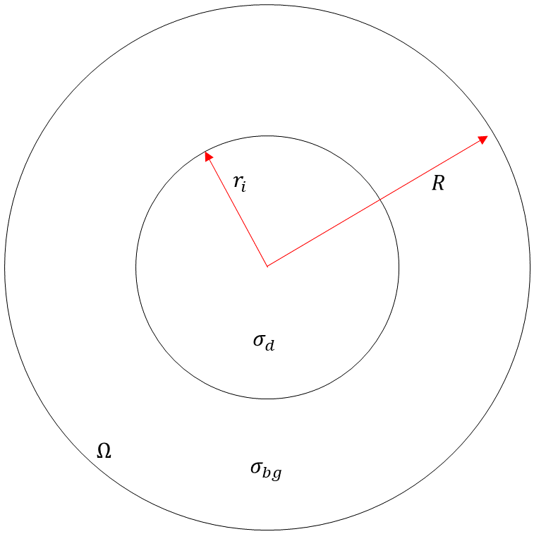
The geometry considered is the one in Figure 1, with two concentric circles characterized by two different homogeneous electrical conductivities. The aim is to recover the shape of the internal inclusion, i.e. the unknown radius . For this geometry, it is possible to analytically evaluate the operator with its eigenvalues and eigenfunctions.
Using the polar coordinates , if is the applied current flux at boundary, then
| (5.1) |
with
The eigenvalues are
Following the algorithm presented at the end of Section 4, problem (2.1) is solved for an electrical conductivity equal to and an eigenfunction of as boundary data. For this particular case, the eigenfucnctions take the form . The corresponding electric scalar potential is
and the related power density
The internal inclusion is reconstructed as the region in which , where is a proper constant. A possible choice of is given by the fact that, for small values of , all the power difference can be reasonably assumed as concentrated in the region occupied by the anomaly. In other words, the conjecture is that
As already discussed in 4, the power difference , when the current flux at the boundary is an eigenfunction of , is related to eigenvalues by the relationship
Summarizing, the problem becomes find such that
This led to
and, hence,
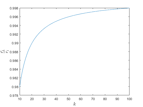
In Figure 2 the behaviour of with respect to the order of the selected eigenvalue is reported, for , , and . As it can be seen, the reconstructed radius tends to the true internal radius as . The Figure shows also that, considering a relatively low , it is possible to achieve a good reconstruction.
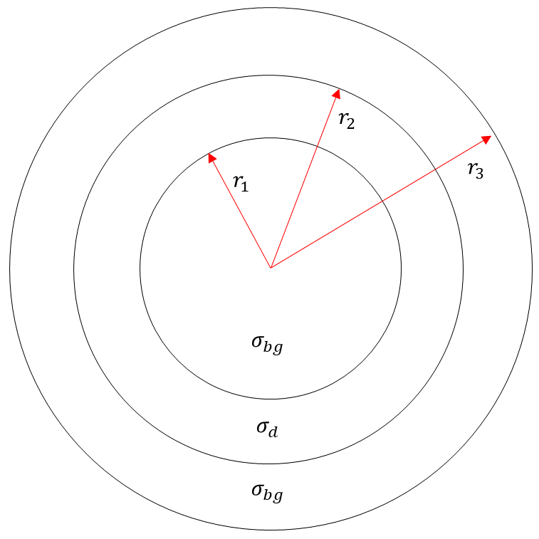
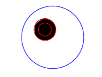
In the following, a second case of an hollow anomaly is considered. Specifically, the reference geometry is the one of Figure 3, where the anomaly is given by the circular crown with internal radius and external radius .
Also in this case, the NtD operator takes the form (5.1), with
The eigenvalues are
Applying the Kernel Method in the same way of the previous case, the power density (on the reference configuration) is evaluated when the system is driven by the eigenfunction , obtaining
| (5.2) |
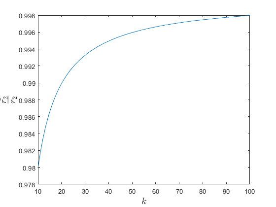
The power density in (5.2) is a monotonic function of the radius . This implies that it is not possible to correctly reconstruct the circular crown. However, the application of the Kernel Method allows to find the the external radius of the anomaly. Repeating the same calculation of the previous case, it follows
that approaches to for .
Remark 5.1.
The impossibility to correct reconstruct hollow anomalies derives from an intrinsic limit of the physical problem considered. Indeed, the fundamental requirement to reconstruct an anomaly is the possibility to find a proper excitation on able to produce an electric current density flowing in all the domain but not in the region . In the case of Figure 3, there is any path for the current density reaching the internal circle of radius without crossing the anomaly .
6. Treatment of the noise
In this section, the application of the Kernel Method in the presence of noisy measurements is treated. Without loss of generality, the following noise model is adopted
| (6.1) |
where is a bounded operator.
From standard arguments of perturbation theory for linear operators, it is possible to prove the following result [24]
Proposition 6.1.
Let , as defined in (6.1), with . Let , the eigenvalues of and , respectively, ordered in a decreasing order. Then
Proposition 6.1 allows to quantitatively evaluate the impact of the noise on the eigenvalues of the key operator . Specifically, given the noise level as the 2-norm of the noise operator , the eigenvalues of differ at most from the corresponding eigenvalues of the unperturbed operator. It follows that all the eigenvalues with amplitude less than , and the corresponding eigenfunctions, are not reliable because they are highly corrupted by noise.
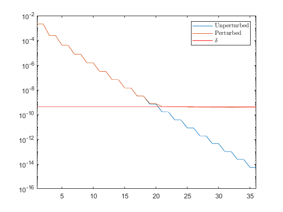
As it can be seen in Figure 5, the eigenvalues of the perturbed operator plateauing when their amplitude is comparable with and they stop to follow the eigenvalues of the unperturbed operator. Some similar consideration about the impact of noise on the spectrum of can also be found in [25].
The analytical examples of Section 5 suggest that the quality of reconstructions increases with the order of the selected eigenfunction (see Figure 2 and 4). As a consequence, the idea is to identify the smallest reliable eigenvalue and to drive the system with the corresponding eigenfunction.
The plateau of the eigenvalues around the noise level causes an abrupt change in the slope of the curve, depicted in Figure 5, which makes easy to identify the reliable eigenvalues.
In the last part of this section, a more detailed discussion about the choice of the threshold follows. Specifically, clear bounds for admissible values of can be analytically derived. The starting point is the following inequality (see proof of 3.1)
Let us suppose that , then
| (6.2) |
with and . Finally, let to be an eigenfunction of , then
So the threshold has to be chosen as
| (6.3) |
where .
Remark 6.2.
In the following, the Kernel Method is summarized
-
•
Compute experimentally or numerically .
-
•
Measure (a noisy version of)
-
•
Find the eigenvalues and the eigenfunctions of .
-
•
Identify the last eigenvalue of before the plateau and the corresponding eigenfunction
-
•
Solve the problem (2.1) when the conductivity is and the applied curent flux at boundary is .
-
•
The reconstructed anomaly is the region for which
(6.4)
Remark 6.3.
The evaluation of the reconstructed anomaly consists in: (i) setting a starting value , (ii) computing the integral on , (iii) increasing and computing the integral until condition (6.4) is fulfilled.
7. Numerical Examples
In this section, the Kernel Method is applied to some practical cases in order to show the effectiveness of the proposed approach. The data are obtained by means of an in-house FEM code, based on the Galerkin method. The domain is a circle with radius and it is discretized in triangular elements, while the boundary is given by elements of the same length. The mesh has nodes. The electric potential is discretized with a piece-wise linear function, as the boundary potential, while the imposed normal component of current density is discretized by a piece-wise constant function on the boundary elements. In this discrete setting, the NtD operator is a linear map from the values of on the boundary elements to the values of the boundary potential on the boundary nodes.
All the reconstructions are obtained by adding synthetic noise on the data. Specifically, we adopt the following noise model, which is the transposition of the one presented in (6.1), for continuous operators, to matrices
where and are the numerical counterparts of the operators and , respectively, and is the noisy version of .
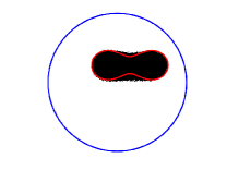
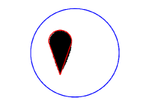
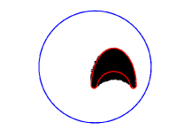
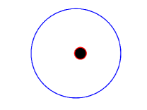
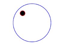
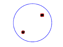
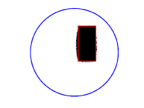
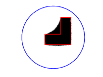
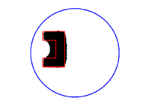
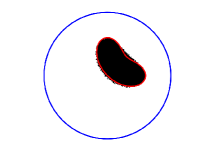
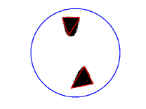
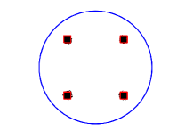
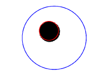
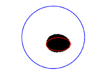
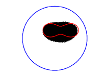
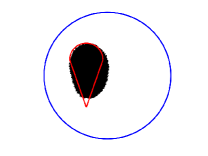
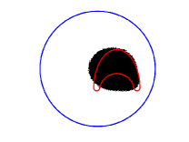
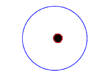
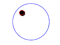
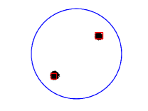
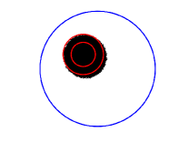
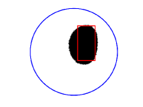
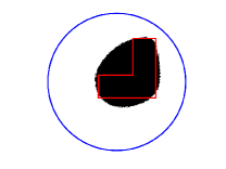
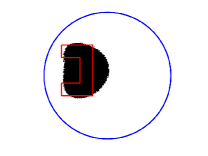
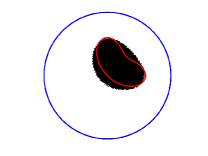
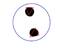
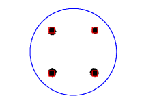
The background material has uniform electrical conductivity equal to while the electrical conductivity of the anomaly is equal to . The reconstructions are reported in Figure 6 and 7. From these Figures, it is possible to infer that, at a realistic noise level, the reconstructions are of high quality. Specifically, we highlight (i) excellent performances on convex anomalies (A, B, D, F, G, J), (ii) possibility of resolving multiple anomalies (H, N, O), (iii) tendency to convexification (C, E, I, K, L, M), and (iv) impossibility to reconstruct the interior of an anomaly with cavities (I).


8. Conclusions
In this work, a new non-iterative imaging method for Electrical Resistance Tomography is presented. Specifically, the method is meant for the inverse obstacle problem, where the aim to retrieve an unknown anomaly embedded in a known background. The method relies on the possibility to find a boundary data producing a vanishing electric field in the regions occupied by the anomaly, when it drives a reference configuration without anomaly.
We provide a simple manner to evaluate this special boundary data and from this we derive a new algorithm with a very simple numerical implementation and very low computational cost.
The numerical examples shows that the proposed algorithm can achieve good performance also in presence of noise to which it appears to be quite robust.
References
- [1] Cheng J, Liu S and Li Y 2019 Design and optimization of liquid level sensor based on electrical tomography 2019 IEEE International Conference on Imaging Systems and Techniques (IST) pp 1–6
- [2] Durdevic P, Hansen L, Mai C, Pedersen S and Yang Z 2015 IFAC-PapersOnLine 48 147–153 ISSN 2405-8963 2nd IFAC Workshop on Automatic Control in Offshore Oil and Gas Production OOGP 2015
- [3] Mann R 2009 Ert imaging and linkage to cfd for stirred vessels in the chemical process industry 2009 IEEE International Workshop on Imaging Systems and Techniques pp 218–222
- [4] Holder D 1994 Thorax 49 626–626
- [5] Kruger M V P 2003 Tomography as a metrology technique for semiconductor manufacturing Tech. Rep. UCB/ERL M03/11 EECS Department, University of California, Berkeley
- [6] Jordana J, Gasulla M and Pallàs-Areny R 2001 Measurement Science and Technology 12 1061–1068
- [7] Hou T C, Loh K J and Lynch J P 2007 Nanotechnology 18 315501
- [8] Linderholm P, Marescot L, Loke M H and Renaud P 2008 IEEE Transactions on Biomedical Engineering 55 138–146
- [9] Cheney M, Isaacson D and Newell J C 1999 SIAM Review 41 85–101
- [10] Brühl M 2001 SIAM Journal on Mathematical Analysis 32 1327–1341
- [11] Ikehata M 2000 Inverse Problems 16 785–793
- [12] Friedman A and Vogelius M 1989 Archive for Rational Mechanics and Analysis 105 299–326
- [13] Tamburrino A and Rubinacci G 2002 Inverse Problems 18 1809–1829
- [14] Tamburrino A, Rubinacci G, Soleimani M and Lionheart W 2003 3rd World Congress on Industrial Process Tomography
- [15] Tamburrino A 2006 Journal of Inverse and Ill-posed Problems 14 633–642
- [16] Gisser D G, Isaacson D and Newell J C 1990 SIAM Journal on Applied Mathematics 50 1623–1634
- [17] Calderon A P 1980 On an inverse boundary Seminar on Numerical Analysis and its Applications to Continuum Physics, Rio de Janeiro, 1980 (Brazilian Math. Soc.) pp 65–73
- [18] Gebauer B 2008 Inverse Problems & Imaging 2 251–269
- [19] Harrach B and Ullrich M 2013 SIAM Journal on Mathematical Analysis 45 3382–3403
- [20] Ikehata M 1998 Journal of Inverse and Ill-Posed Problems 6 127–140
- [21] Alessandrini G 2012 Journal of Mathematical Analysis and Applications 386 669–676 ISSN 0022-247X
- [22] Garofalo N and Lin F 1986 Indiana University Mathematics Journal 35 245–268
- [23] Rudin W 1991 Functional Analysis 2nd ed International series in pure and applied mathematics (McGraw-Hill) ISBN 0070542368; 9780070542365
- [24] Kato T 1995 Perturbation theory for linear operators Classics in Mathematics (Springer) ISBN 9783540586616,354058661X
- [25] Brühl M and Hanke M 2000 Inverse Problems 16 1029–1042