A Unified Framework for Unsupervised Domain Adaptation based on Instance Weighting

Abstract

Despite the progress made in domain adaptation, solving Unsupervised Domain Adaptation (UDA) problems with a general method under complex conditions caused by label shifts between domains remains a formidable task. In this work, we comprehensively investigate four distinct UDA settings including closed set domain adaptation, partial domain adaptation, open set domain adaptation, and universal domain adaptation, where shared common classes between source and target domains coexist alongside domain-specific private classes. The prominent challenges inherent in diverse UDA settings center around the discrimination of common/private classes and the precise measurement of domain discrepancy. To surmount these challenges effectively, we propose a novel yet effective method called Learning Instance Weighting for Unsupervised Domain Adaptation (LIWUDA), which caters to various UDA settings. Specifically, the proposed LIWUDA method constructs a weight network to assign weights to each instance based on its probability of belonging to common classes, and designs Weighted Optimal Transport (WOT) for domain alignment by leveraging instance weights. Additionally, the proposed LIWUDA method devises a Separate and Align (SA) loss to separate instances with low similarities and align instances with high similarities. To guide the learning of the weight network, Intra-domain Optimal Transport (IOT) is proposed to enforce the weights of instances in common classes to follow a uniform distribution. Through the integration of those three components, the proposed LIWUDA method demonstrates its capability to address all four UDA settings in a unified manner. Experimental evaluations conducted on three benchmark datasets substantiate the effectiveness of the proposed LIWUDA method.

I Introduction

Deep neural networks (DNNs) have demonstrated remarkable advancements across various applications, such as image classification [1], object detection [2], and semantic segmentation [3]. Nevertheless, due to the data-driven nature of DNNs, the pronounced reliance on annotated in-domain data imposes significant constraints on their effectiveness in cross-domain scenarios. To surmount this challenge, Unsupervised Domain Adaptation (UDA) [4] has emerged as a viable remedy by facilitating the transfer of knowledge from a labeled source domain to an unlabeled target domain. UDA has witnessed substantial strides across multiple applications [5, 6, 7, 8, 9] and most UDA models operate under the Closed Set Domain Adaptation (CSDA) setting, where both domains share an identical label space as shown in Figure 1(a). However, this assumption often proves impractical in real-world applications. To alleviate the limitations of the CSDA setting, several alternative settings have been proposed, including Partial Domain Adaptation (PDA) [10, 11], Open Set Domain Adaptation (OSDA) [12], and Universal Domain Adaptation (UniDA) [13]. Specifically, PDA assumes that the label space of the target domain is a subset of that in the source domain, while OSDA takes the converse assumption that the label space of the source domain is a subset of that in the target domain. UniDA, residing between these extremes, assumes that the label spaces of the two domains exhibit some degree of overlap. As illustrated in Figure 1, these three settings collectively contribute valuable strides towards enhancing the practical applicability of UDA.

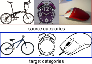
(a) Closed Set Domain Adaptation

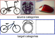
(b) Partial Domain Adaptation

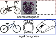
(c) Open Set Domain Adaptation

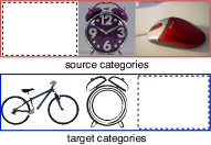
(d) Universal Domain Adaptation

Figure 1: Four UDA settings with respect to labels of source and target domains. Real pictures in the first row of each figure represent several categories in the source domain and clipart pictures in the second row denote categories in the target domain. A dashed rectangle indicates the absence of categories within one domain, which conversely exists within the other domain.

As introduced in Section II, existing works typically focus on solving each individual UDA setting by proposing distinct methodologies. While those methods have attained remarkable achievements within their specific UDA settings, their effectiveness becomes insufficient within intricate application contexts, necessitating the formulation of a unified framework to address different UDA settings.

Hence, this study endeavors to construct a unified framework capable of resolving diverse UDA settings. However, this endeavor is met with two pivotal challenges. The first challenge is how to effectively differentiate common classes shared across domains from domain-specific private classes during the cross-domain knowledge transfer and the second one is how to achieve the alignment between two domains characterized by dissimilar label spaces.

To address those challenges, we propose a novel yet effective method called Learning Instance Weighting for Unsupervised Domain Adaptation (LIWUDA) that undertakes the identification and alignment of common classes within two domains. Specifically, the proposed LIWUDA method commences with the design of a weight network to assign weights to individual instances, thereby measuring the probability of instance belonging to common classes. Subsequently, by leveraging these instance weights, we propose the Weighted Optimal Transport (WOT), which effectively minimizes the transportation cost from the source domain to the target domain, facilitating the domain alignment. To separate instances with low similarities and align samples with high similarities, we put forth the Separate and Align (SA) loss, underpinned by a comparison of similarities against the mean cost of WOT. Finally, to guide the learning of the weight network, we introduce the Intra-domain Optimal Transport (IOT) based on WOT to transport one domain, which has only common classes, to itself with a uniform data distribution. In this way, we provide auxiliary information to help learn the weight network. By combining these strategies, the proposed LIWUDA method culminates in a unified framework that comprehensively addresses the four distinctive UDA settings, effectively discovering shared common classes and mitigating domain divergence.

In summary, our main contributions are four-fold. (I) We introduce the unified LIWUDA framework, proficiently addressing four distinct UDA settings. (II) We propose a weight network to assign instance weights, quantifying the probability of an instance belonging to common classes, and subsequently employ this weighting mechanism to devise the WOT strategy, effectively mitigating the domain divergence between the source and target domains. (III) We innovate the SA loss, effectively segregating and aligning samples to harness the cost of WOT, complemented by the IOT, which furnishes auxiliary information for the training of the weight network. (IV) Extensive experiments are conducted to verify the effectiveness of the proposed LIWUDA method across varying UDA settings.

II Related Work

Closed Set Domain Adaptation. In CSDA, where the source and target domains are assumed to share an identical label space, the primary research focus lies in mitigating distributional disparities across domains by learning domain-invariant feature representations. This pursuit involves two primary strategies. Specifically, the first strategy capitalizes on statistic moment matching, exemplified by methods such as Maximum Mean Discrepancy (MMD) [14, 15], central moment discrepancy [16], and second-order statistics matching [17]. The second strategy involves adversarial learning paradigms that foster indistinguishability of samples across domains concerning domain labels, typified by domain adversarial neural network and its extensions [18, 19]. The applicability of CSDA methods to other UDA settings featuring disparate label spaces across domains is not straightforward. Differently, we propose the unified LIWUDA framework, which adeptly accommodates four distinct UDA settings by leveraging the proposed weight network.

Partial Domain Adaptation. Within the PDA paradigm, the assumption is that the source domain encompasses private classes that does not exist in the target domain, and several methods have been proposed. For instance, PADA [20] assigns decreased weight to private classes in the source domain, while IWAN [21] devises a weight assignment mechanism facilitated by an adversarial network to discern samples from private classes. Similarly, SAN [22] employs adversarial learning to identify private classes in the source domain, and ETN [23] designs a progressive weighting scheme to quantify the transferability of source instances. DRCN [24], on the other hand, introduces a weighted class-wise matching strategy, explicitly aligning target instances with the most relevant source classes. Diverging from those methodologies, we propose WOT for the purpose of source instance weighting, thereby alleviating the deleterious effects brought by private classes in the source domain.

Open Set Domain Adaptation. In this work, we mainly focus on the OSDA setting proposed in [12], where the target domain encompasses private classes unfamiliar to the source domain. The prevailing objective among OSDA methodologies centers on the identification and exclusion of outliers originating from private classes in the target domain, subsequently reducing the domain gap between source instances and target inliers belonging to common classes. For instance, OSBP [12] proposes an adversarial learning framework to enable the feature generator to acquire representations conducive to the delineation between common and private classes in the target domain. Likewise, ROS [25] employs a self-supervised learning approach, adeptly achieving dual objectives of separating common/private classes in the target domain and aligning domains. In contrast, the proposed LIWUDA method leverages the weights obtained from the weight network to discriminate whether each target instance is affiliated with private classes.

Universal Domain Adaptation. As a much challenging setting, UniDA introduces a heightened level of complexity by accommodating private classes within both domains. [13] proposes the UniDA framework, which eschews the necessity for prior knowledge of label space in two domains and introduces the Universal Adaptation Network (UAN) to classify whether each target instance is in common classes. CMU [26] combines the entropy, confidence, and consistency metrics to effectively gauge the proclivity of a target instance towards private classes in the target domain, thereby enabling the detection of private classes and accurate classification of data within common classes of the two domains. Similarly, [27] introduces neighborhood clustering and entropy separation to learn discriminative feature representations for target instances. Notwithstanding these advancements, all these models overlook the predilection of source instances towards private classes in the source domain, potentially leading to suboptimal performance. In contrast, the proposed LIWUDA model introduces the SA loss, designed to effectively separate instances with low similarities and align instances with high similarities across domains.

Optimal Transport. Optimal transport (OT) is initially introduced by [28], originated as an efficient technique for redistributing mass distributions. In recent years, OT has been harnessed extensively within the domain adaptation domain [29, 30, 31, 32, 33, 34, 35, 36, 37, 38, 39], aligning the source and target domains by optimizing the coupling matrix to minimize the cost of transporting from the source domain to the target domain. Among those works, a representative one is DeepJDOT [36], which employs the learned optimal transport coupling matrix to align two domains in the learned feature space. Additionally, advancements have led to new optimal transport algorithms such as [40], which incorporates label information through a combination of matrix scaling and non-convex regularization. The SWD method [41] captures the inherent dissimilarities between outputs of task-specific classifiers, enabling the effective detection of target samples distant from the support of the source domain and facilitating end-to-end distributional alignment. RWOT [37] designs an integration of shrinking subspace reliability and a discriminative centroid loss. Different from the aforementioned models that only handle the CSDA setting, we introduce WOT built upon optimal transport, thereby enabling the proposed method to effectively address four distinct scenarios in UDA. Through the utilization of the WOT, we propose the SA loss to successfully separate and align instances, which is bolstered by the IOT loss that imparts auxiliary insights for obtaining weights of instances. As a culmination, the proposed model adeptly tackles the challenges of discriminating common and domain-specific classes, while also accurately quantifying domain divergence.

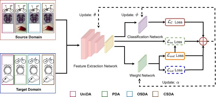
Figure 2: Illustration of LIWUDA. Input data varies based on the UDA setting, indicated by different colors representing UniDA, PDA, OSDA, and CSDA. Instance feature representations are obtained through the feature extraction network $f(\cdot;\theta)$. Those representations are then utilized as inputs for both the classification network $h(\cdot;\phi)$ and the weight network $w(\cdot;\alpha)$ to obtain predictions and instance weights. The classification loss $\mathcal{L}_{\mathcal{C}}$ is computed using labeled source instances. By utilizing the feature representations and instance weights, we calculate the cost of WOT $\mathcal{L}_{wot}$. Additionally, we formulate the SA loss $\mathcal{L}_{sa}$ by leveraging the feature representation and $\mathcal{L}_{wot}$. The incorporation of the IOT loss $\mathcal{L}_{iot}$ aids in guiding the training of the weight network. A dashed box denotes potential inapplicability of the corresponding loss in certain settings.

III The LIWUDA Method

In this section, we present the proposed LIWUDA method.

III-A Problem Settings

In UDA, we are given a labeled source domain $D_{s}=\{{(x_{i}^{s},y_{i}^{s})}\}_{i=1}^{n_{s}}$ with $n_{s}$ instances and an unlabeled target domain $D_{t}=\{{{x}_{j}^{t}}\}_{j=1}^{n_{t}}$ with $n_{t}$ unlabeled instances. The label spaces of the source and target domains are respectively denoted by $C_{s}$ and $C_{t}$, with differing data distributions characterizing the source and target domains.

In the UniDA setting, $C=C_{s}\cap C_{t}$ represents the nonempty set of common classes shared by both domains. Meanwhile, $\bar{C}_{s}=C_{s}\setminus C$ and $\bar{C}_{t}=C_{t}\setminus C$ denote the sets of private classes exclusive to the source and target domains. The aim of UniDA is to accurately predict target instances in $C$ and adeptly discern target instances within $\bar{C}_{t}$.

In the context of PDA, the label space $C_{s}$ in the source domain is a superset of $C_{t}$ in the target domain, i.e., $C_{t}\subset C_{s}$. By detecting the set of source-private classes $\bar{C}_{s}=C_{s}\setminus C_{t}$, the essence of PDA lies in precise prediction for the target domain.

Under the OSDA setting, the label space in the source domain is a subset of that in the target domain, i.e., $C_{s}\subset C_{t}$. Consequently, the target domain introduces a set of private classes $\bar{C}_{t}=C_{t}\setminus C_{s}$, often referred to as $unknown$ classes, owing to the dearth of prior knowledge. Much like UniDA, OSDA strives for accurate predictions within $C_{s}$ for target instances, while distinguishing those within $\bar{C}_{t}$.

In the CSDA setting, both domains share identical label sets $C_{s}=C_{t}$. The core objective revolves around domain alignment, enabling a model trained within the labeled source domain to be effectively employed for the target domain.

III-B The Framework

As illustrated in Figure 2, the architecture of the LIWUDA method comprises a triad of pivotal components: a feature extraction network $f(\cdot;\theta)$, a classification network $h(\cdot;\phi)$, and a weight network $w(\cdot;\alpha)$. The feature extraction network $f(\cdot;\theta)$ parameterized by $\theta$ transforms each data instance into a latent representation. Concurrently, the classification network $h(\cdot;\phi)$ parameterized by $\phi$ leverages the output of $f(\cdot;\theta)$ to form predictions. The weight network $w(\cdot;\alpha)$ characterized by $\alpha$ processes the output of $f(\cdot;\theta)$ to generate a scalar weight representing the probability of an instance belonging to the shared common classes in either the source or target domain or both. To confine the output to the range of $[0,1]$, a sigmoid function is applied at the top of the weight network $w(\cdot;\alpha)$. Furthermore, the computation of a normalized output, $\hat{w}(\cdot;\alpha)$, is essential, ensuring that $\sum_{x\in D}\hat{w}(x;\alpha)=1$ within dataset $D$, designated as $D_{s}$ or $D_{t}$. For notation simplicity, we omit the dependency of the four functions with respect to model parameters and denote them by $f(\cdot)$, $h(\cdot)$, $w(\cdot)$, and $\hat{w}(\cdot)$.

Based on the architecture introduced above, the LIWUDA method formulates its central objective, characterized by the integration of four distinct loss functions, as

$$\mathcal{L}=\mathcal{L}_{\mathcal{C}}+\beta\mathcal{L}_{wot}+\eta\mathcal{L}_{sa}+\epsilon\mathcal{L}_{iot},$$ (1)

where $\beta$, $\eta$, and $\epsilon$ are nonnegative hyperparameters. In the following, we introduce the four losses used in Eq. (1) in a step-by-step manner.

The first loss $\mathcal{L}_{\mathcal{C}}$ represents the classification loss on the labeled source domain and it is formulated as

$$\mathcal{L}_{\mathcal{C}}=\frac{1}{n_{s}}\sum_{i=1}^{{n}_{s}}\ell\left(h(f(x^{s}_{i})),{y}_{i}^{s}\right),$$ (2)

where $h(f(x^{s}_{i}))$ denotes the classification probability for the $i$-th source instance $x^{s}_{i}$ based on the feature extraction and classification networks, and $\ell(\cdot,\cdot)$ denotes the cross-entropy loss function.

III-B1 Weighted Optimal Transport

In this work, our objective is to introduce a comprehensive framework capable of addressing all four UDA scenarios. However, given the presence of domain-specific classes, direct domain alignment between domains can lead to negative transfer. To mitigate this issue, we introduce a weight network that evaluates the probability of instances belonging to common classes. By leveraging instance weights and optimal transport for UDA [29, 30, 31, 32, 33], we devise a novel approach termed Weighted Optimal Transport (WOT) to effectively measure the domain divergence across all UDA settings. Building upon the acquired feature representations and instance weighting, the WOT cost denoted by $\mathcal{L}_{wot}$ is formulated as

$$\mathcal{L}_{wot}={\left\langle{{\gamma}^{*}},\mathcal{D}({X}^{s},{X}^{t})\right\rangle}_{F},$$ (3)

where ${\left\langle\cdot,\cdot\right\rangle}_{F}$ is the Frobenius dot product, $\gamma^{*}$ is the optimal coupling matrix between the source and target domains, ${X}^{s}$ and ${X}^{t}$ refer to the data in the source and target domains, respectively, and $\mathcal{D}({X}^{s},{X}^{t})$ denotes the cost of transport from $X^{s}$ to $X^{t}$. Here $\mathcal{D}({X}^{s},{X}^{t})$ is represented by an $n_{s}\times n_{t}$ dissimilarity matrix with the $(i,j)$-th element defined as $\mathcal{D}\left({x}^{s}_{i},{x}^{t}_{j}\right)=1-\frac{\left\langle f({x}^{s}_{i}),f({x}^{t}_{j})\right\rangle}{\lVert f(x^{s}_{i})\rVert_{2}{\lVert f(x^{t}_{j})\rVert_{2}}}$, where $\|\cdot\|_{2}$ denotes the $\ell_{2}$ norm of a vector.

The optimal coupling matrix $\gamma^{*}$ in Eq. (3) is computed through the subsequent Kantorovitch problem [28] as

$${\gamma}^{*}=\mathop{\arg\min}_{\gamma\in\mathcal{B}(p(X^{s}),p(X^{t}))}{\left\langle\gamma,\mathcal{D}({X}^{s},{X}^{t})\right\rangle}_{F},$$ (4)

where $\bm{1}_{d}$ is a $d$-dimensional vector of all ones, the superscript ^⊤ denotes the transpose operation, $p(X^{s})$ defines a discrete probability distribution for source instances in $X^{s}$ by satisfying $p(X^{s})\geq 0$ and $p(X^{s})^{\top}\mathbf{1}_{n_{s}}=1$, $p(X^{t})$ is defined similarly for $X^{t}$, and given $p_{1}\in\mathbb{R}_{+}^{n_{s}}$ and $p_{2}\in\mathbb{R}_{+}^{n_{t}}$ satisfying $p_{1}^{\top}\mathbf{1}_{n_{s}}=1$ and $p_{2}^{\top}\mathbf{1}_{n_{t}}=1$, $\mathcal{B}(p_{1},p_{2})$ denotes the set of coupling matrices as

$$\mathcal{B}(p_{1},p_{2})=\{\gamma\in\mathbb{R}_{+}^{n_{s}\times n_{t}}\mid\gamma\bm{1}_{n_{t}}=p_{1},\gamma^{\top}\bm{1}_{n_{s}}=p_{2}\}.$$ (5)

In the original optimal transport, $p(X^{s})=\bm{1}_{n_{s}}/{n_{s}}$ and $p(X^{t})=\bm{1}_{n_{t}}/{n_{t}}$ remain constant if there is no prior information regarding the data distribution. In contrast, within the proposed WOT, $p(X^{s})$ and $p(X^{t})$ can either adopt values from $\hat{w}(\cdot)$ or remain constant, contingent upon the specific UDA setting being addressed, as elucidated in the subsequent section. In this light, it can be inferred that the optimal transport concept emerges as a special instance of the proposed WOT methodology.

III-B2 Separate and Align

While the measurement of domain divergence through the cost computation of WOT is feasible, the presence of domain-private classes may introduce less reliable estimation for the domain divergence. Drawing inspiration from JPOT [42], we harness the WOT cost (i.e., $\mathcal{L}_{wot}$) as a means to effectively manage the separation and alignment of data across domains. Specifically, we employ $\mathcal{L}_{wot}$ to gauge the distance between each coupled instance pair, thereby guiding the decision to separate or align these instances. When the distance between a coupled pair surpasses $\mathcal{L}_{wot}$, it signifies the infeasibility of transferring knowledge between that pair. Computation of the $(i,j)$-th element within the partial coupling matrix for domain alignment can be defined as

$$\hat{\gamma}^{*}_{i,j} =\gamma_{i,j}^{*}\times\pi(x_{i}^{s},x_{j}^{t},\mathcal{L}_{wot}),$$ (6)

$$\pi(x_{i}^{s},x_{j}^{t},\mathcal{L}_{wot}) =1-\frac{1}{2}\left(1+\operatorname{sgn}\left(\mathcal{D}\left(x_{i}^{s},x_{j}^{t}\right)-\mathcal{L}_{wot}\right)\right),$$

where $\operatorname{sgn}(x)$ equals 1 when $x>0$, and equals $-1$ otherwise. It is easy to see that $\hat{\gamma}^{*}_{i,j}$ equals 0 if $\mathcal{D}\left(x_{i}^{s},x_{j}^{t}\right)>\mathcal{L}_{wot}$ and otherwise $\gamma^{*}_{i,j}=1$. Then, the Separate and Align (SA) loss corresponding to the third loss in Eq. (1) for separating and aligning data based on the WOT is formulated as

$$\mathcal{L}_{sa}=\sum_{i,j}\Delta\gamma_{i,j}^{*}(2-\mathcal{D}({x}^{s}_{i},{x}^{t}_{j}))+\sum_{i,j}\hat{\gamma}_{i,j}^{*}\mathcal{D}({x}^{s}_{i},{x}^{t}_{j}),$$ (7)

where $\Delta\gamma_{i,j}^{*}=1-\exp(-(\gamma_{i,j}^{*}-\hat{\gamma}_{i,j}^{*}))$. In Eq. (7), the first term is to separate data with large dissimilarities from two domains and the second term is to align data from two domains with small dissimilarities.

III-B3 Intra-domain Optimal Transport

Furthermore, it becomes evident that target instances (or source instances) within the context of the PDA (or OSDA) setting inherently belong to common classes, and their weights could be approximated to be equal without relying on prior information. This particular insight can be harnessed to guide the learning process of the weight network. To achieve this, we employ the Intra-domain Optimal Transport (IOT) technique within the target domain (or source domain). To elaborate, for a given set of $n$ examples denoted as $X=\{x_{i}\}_{i=1}^{n}$, we formulate the IOT loss as

$$\mathcal{L}_{iot}={\left\langle{{\kappa}^{*}},\mathcal{D}(X,X)\right\rangle}_{F},$$ (8)

where ${\kappa}^{*}$ is obtained by solving the following problem as

$${\kappa}^{*}=\mathop{\arg\min}_{\kappa\in\mathcal{B}(\hat{w}(X),\bm{1}_{n}/n)}{\left\langle\kappa,\mathcal{D}({X},{X})\right\rangle}_{F}.$$ (9)

In the PDA setting, we have $X=X^{t}$ and $n=n_{t}$, while in the OSDA setting, $X$ corresponds to $X^{s}$ and $n$ equals $n_{s}$. Through problem (9), our objective is to enforce the normalized output of the weight network, which is denoted by $\hat{w}(X)$, towards $\bm{1}_{n}/n$. This problem imparts valuable guiding insights for the effective training of the weight network.

III-B4 Entire Objective Function

In summary, the LIWUDA method is to determine the optimal coupling matrices $\gamma^{*}$ and $\kappa^{*}$, alongside the minimization of the objective function $\mathcal{L}$. By amalgamating these critical components, the complete objective function of the proposed LIWUDA approach is formulated as

$$\min_{\theta,\phi,\alpha} \ \leavevmode\nobreak\ \mathcal{L}=\mathcal{L}_{\mathcal{C}}+\beta\mathcal{L}_{wot}+\eta\mathcal{L}_{sa}+\epsilon\mathcal{L}_{iot}$$ (10)

s.t $$\ \leavevmode\nobreak\ \gamma^{*}=\mathop{\arg\min}_{\gamma\in\mathcal{B}(p(X^{s}),p(X^{t}))}\mathcal{L}_{wot},$$

$$\ \leavevmode\nobreak\ \kappa^{*}=\mathop{\arg\min}_{\kappa\in\mathcal{B}(\hat{w}({x}),\bm{1}_{n}/{n})}\mathcal{L}_{iot}.$$

Problem (10) is a bi-level optimization problem [43] and we can use the Stochastic Gradient Descent (SGD) method or its variants to solve it as [44, 45] did.

III-C Applications to Different UDA Settings

Problem (10) presents a general formulation for UDA. However, owning to the distinct attributes associated with common classes across the four UDA settings, there can be variations in the configuration of the objective function $\mathcal{L}$ and the ensemble of coupling matrices. In the forthcoming sections, we delve into the specifics of each individual setting.

III-C1 Universal Domain Adaptation

In the UniDA setting, it is notable that both the source and target domains contain private classes, thereby instigating the weight network to apportion weights to instances from both domains. This prompts the setting of $p(X^{s})=\hat{w}({X}^{s})$ and $p(X^{t})=\hat{w}({X}^{t})$ in problem (4). Notably, given the absence of a prior knowledge concerning common classes shared between the two domains, the utilization of $\mathcal{L}_{iot}$ to steer the weight network’s learning process is omitted, thus setting the hypeparameter $\epsilon=0$.

III-C2 Partial Domain Adaptation

In the PDA setting, it is worthy noting that solely the source domain comprises private classes, thereby confining the weight network to weighing instances exclusively within the source domain. Consequently, it becomes apt to assign $p(X^{s})=\hat{w}({X}^{s})$ and $p(X^{t})=\bm{1}_{n_{t}}/{n_{t}}$ in relation to problem (4). Noteworthy also is the fact that, due to the encompassing presence of common classes in the target domain, all instances within this domain are endowed with similar weights. Hence $X$ and $n$ in problem (9) are set to $X^{t}$ and $n_{t}$, respectively.

III-C3 Open Set Domain Adaptation

In contrast to the PDA setting, the OSDA configuration takes a converse stance, as the source domain exclusively comprises common classes. As such, it becomes apt to establish $p(X^{t})=\hat{w}({X}^{t})$ and $p(X^{s})=\bm{1}_{n_{s}}/{n_{s}}$ in connection with problem (4). Furthermore, for the IOT stipulated by problem (9), the choice of $X$ and $n$ finds its alignment with $X^{s}$ and $n_{s}$, respectively.

III-C4 Closed Set Domain Adaptation

The CSDA setting is easier than the other three settings as there is no private class in both domains. Hence, there is no need to use the weight network to weigh instances in both domains, and we do not need $\mathcal{L}_{sa}$ and IOT by setting $\eta=0$ and $\epsilon=0$. As a consequence, we set $p(X^{s})=\bm{1}_{n_{s}}/{n_{s}}$ and $p(X^{t})=\bm{1}_{n_{t}}/{n_{t}}$ in problem (4), making WOT reduce to optimal transport, and the entire LIWUDA method becomes OT-based approaches for UDA (e.g., OTDA [29] and JDOT [30]). Hence, we do not report experimental results on the CSDA setting in Section IV.

In summary, Table I serves to concisely delineate the divergent formulations applied across the four UDA settings. Remarkably, LIWUDA emerges as an overarching framework capable of accommodating all the four UDA settings. The training regimen of the LIWUDA method is elucidated through Algorithms 1. Moreover, for the OSDA and UniDA settings, Algorithm 2 comprehensively delineates the inference process, where the output of the weight network is used to identify whether a sample is from a common or private class.

Table I: Comparison of formulations for four UDA settings.

Setting	$\mathcal{L}_{\mathcal{C}}$	$\mathcal{L}_{wot}$	$\mathcal{L}_{sa}$	$\mathcal{L}_{iot}$	Problem (4)		Problem (9)
					$p(X^{s})$	$p(X^{t})$	$X$	$n$
UniDA	$\surd$	$\surd$	$\surd$		$\hat{w}({X}^{s})$	$\hat{w}({X}^{t})$	-	-
PDA	$\surd$	$\surd$	$\surd$	$\surd$	$\hat{w}({X}^{s})$	$\bm{1}_{n_{t}}/{n_{t}}$	$X_{t}$	$n_{t}$
OSDA	$\surd$	$\surd$	$\surd$	$\surd$	$\bm{1}_{n_{s}}/{n_{s}}$	$\hat{w}({X}^{t})$	$X_{s}$	$n_{s}$
CSDA	$\surd$	$\surd$			$\bm{1}_{n_{s}}/{n_{s}}$	$\bm{1}_{n_{t}}/{n_{t}}$	-	-

Algorithm 1 Training process of the LIWUDA framework

1:  Input: $\{X,Y\}$; max iterations: $T$

2:  Initialize parameters of feature extractor $\theta$, those of the classifier $\phi$, and those of the weight network $\alpha$;

3:  for $t=$ 1 to $T$ do

4:     Sample a mini-batch;

5:     Compute the classification loss according to Eq. (2);

6:     Obtain the idea coupling matrix according to Eq. (4);

7:     Compute the WOT loss according to Eq. (3);

8:     Compute the SA loss according to Eq. (7);

9:     Compute the IOT loss according to Eq. (8);

10:     Compute the overall objective according to Eq. (1);

11:     Minimize $\mathcal{L}$ to update $\theta$, $\phi$, and $\alpha$;

12:  end for

13:  return $\theta$, $\phi$, and $\alpha$.

Algorithm 2 Inference process of the LIWUDA framework under the OSDA and UniDA settings

1:  Input: $X$; sample number: $N$

2:  for $n=1$ to $N$ do

3:     Obtain the prediction of a sample: $Y=h(f(x_{n}))$;

4:     Obtain the weight of a sample: $W=w(f(x_{n}))$;

5:     Predict the sample as common or private class:  if $W>0.5$   The sample is labeled as common class;  else   The sample is labeled as private class;

6:     Based on $Y$ and common/private class, make final prediction;

7:  end for

8:  return predictions of samples;

III-D Complexity Analysis

Here, we provide a complexity analysis for the proposed LIWUDA method. Within each iteration, the LIWUDA method necessitates the determination of $\kappa^{*}$ and $\gamma^{*}$ by solving the corresponding problems. By using the mini-batch partial optimal transport method [46], solving such a partial optimal transport problem has a computational complexity $\mathcal{O}(n^{2})$, where $n$ denotes the number of samples. Then for all the parameters $\Theta=\{\theta,\phi,\alpha\}\in\mathbb{R}^{N}$, conducting one-step gradient descent to update them costs $\mathcal{O}(N)$. Therefore, the proposed LIWUDA method has a $\mathcal{O}(N+n^{2})$ computational cost per iteration, which is as the same order as existing OT-based UDA methods [29, 39].

III-E Analysis on Generalization Bound

The LIWUDA method serves as a versatile and unified framework encompassing the four distinct settings within UDA. Beyond its unified formulation for these diverse settings, this framework offers an additional advantage by facilitating the straightforward analysis of critical properties, such as the generalization bound of the LIWUDA method across all four settings. This analysis is the central focus of this section.

The distribution of source domain is represented as $\mu_{s}$ on $\Omega$ and the true labeling function in the source domain is denoted by $f_{s}:\Omega\to[0,1]$. Correspondingly, the distribution of the target domain, alongside its inherent true labeling function, can be established in a similar manner. Let’s consider a set of functions $h\in\mathcal{H}$ that adhere to the constraint $h:\Omega\to\{0,1\}$, wherein $\mathcal{H}$ denotes a reproducing kernel Hilbert space. Given a convex loss function $l$, we can formally define the expected losses pertinent to both the source and target domains as follows:

$$R_{S}(h,f_{s}) =\mathbb{E}_{x\sim\mu_{s}}[l(h(x),f_{s}(x))],$$ (11)

$$R_{T}(h,f_{t}) =\mathbb{E}_{x\sim\mu_{t}}[l(h(x),f_{t}(x))].$$

In the following theorem, we prove a generalization bound for the proposed LIWUDA method under the four UDA settings.

Theorem 1

Suppose the source domain has $n_{s}$ instances, which are drawn i.i.d from the distribution $\mu_{s}$ and stored in $X^{s}$, and the target domain has $n_{t}$ instances, which are drawn i.i.d from the distribution $\mu_{t}$ and stored in $X^{t}$. By assuming that the discrete measures of the source and target data are $p(X^{s})$ and $p(X^{t})$, respectively, we have

$$R_{T}(h,f_{t})\leq R_{S}(h,f_{s})+W\left(p(X^{s}),p(X^{t})\right)+\mathcal{C}+\lambda,$$ (12)

where $\mathcal{C}$ is the combined loss of the ideal hypothesis $h^{*}$ that minimizes the combined loss of $R_{S}(h,f_{s})+R_{T}(h,f_{t})$, $\lambda$ denotes the error between the assumed discrete measure and true distribution on both source and target domains, and the Wasserstein distance $W\left(p(X^{s}),p(X^{t})\right)$ is defined as

$$W\left(p(X^{s}),p(X^{t})\right)=\min_{\gamma\in\mathcal{B}(p(X^{s}),p(X^{t}))}{\left\langle\gamma,\mathcal{D}({X}^{s},{X}^{t})\right\rangle}_{F}.$$

Theorem 1 can be directly deduced from Theorem 2 of [47] by replacing empirical measures of the source and target domains with $p(X^{s})$ and $p(X^{t})$, respectively. In the context of traditional optimal transport [47], the empirical measures of the source and target domain are conventionally set to $\mathbf{1}_{n_{s}}/{n_{s}}$ and $\mathbf{1}_{n_{t}}/{n_{t}}$, respectively. Nevertheless, within the framework of the LIWUDA method, these measures can be flexibly modified through the updates performed on the weight network. This viewpoint underscores that the LIWUDA method not only endeavors to minimize the divergence between the source and target domains, but also strives to discover improved measures for both domains. To elaborate, let $\bar{p}(X^{s})$ and $\bar{p}(X^{t})$ symbolize the optimal discrete measures attributed to the source and target domains, respectively. Consequently, we can establish the following relation:

$$W(\bar{p}(X^{s}),\bar{p}(X^{t})) =\min_{\alpha}W(p(X^{s}),p(X^{t}))$$ (13)

$$\leq W(\mathbf{1}_{n_{s}}/{n_{s}},\mathbf{1}_{n_{t}}/{n_{t}}),$$

where the equality holds due to minimizing $\mathcal{L}_{wot}$ w.r.t $\alpha$ in the LIWUDA method. Note that the above inequality still holds if we fix $p(X^{s})$ as $\mathbf{1}_{n_{s}}/{n_{s}}$ or fix $p(X^{t})$ as $\mathbf{1}_{n_{t}}/{n_{t}}$, and that the right-hand side term of the inequality is just the domain distance in traditional optimal transport. Therefore, the LIWUDA method will have a lower domain distance in all four UDA settings compared with the traditional optimal transport, and this could be a reason of the superior performance of the proposed LIWUDA method under the four UDA settings.

IV Experiments

In this section, we empirically evaluate the proposed LIWUDA method across diverse scenarios including the UniDA, PDA, and OSDA settings.

IV-A Datasets

We conduct comprehensive experiments on three benchmark datasets: Office-31 [48], Office-Home [49], and VisDA [50].

The Office-31 dataset is a widely-used dataset for UDA, which consists of 4652 images of 31 categories from three domains: DSLR (D), Amazon (A), and Webcam (W). We build six tasks to evaluate our method: A$\leftrightarrow$D, A$\leftrightarrow$W, and D$\leftrightarrow$W. The Office-Home dataset is a more challenging dataset, comprising 15,500 images from 65 classes in 4 distinct domains: Artistic images (Ar), Clip-Art images (CI), Product images (Pr), and Real-World images (Rw). We report the performance of all 12 transfer tasks for comprehensive evaluations: Ar$\leftrightarrow$Pr, Ar$\leftrightarrow$Rw, Ar$\leftrightarrow$Rw, Cl$\leftrightarrow$Pr, Cl$\leftrightarrow$Rw, and Pr$\leftrightarrow$Rw. The VisDA dataset, characterized by its large-scale nature, comprises the Synthetic (S) domain containing 152,397 synthetic images and the Real (R) domain with 55,388 images from the real world. By following [51, 26, 52], we construct a task S$\rightarrow$R for the UniDA and OSDA settings, and build two tasks S$\leftrightarrow$R for the PDA setting.

Table II: The split on the label space, i.e., numbers of common classes (C)/ source-private classes ($\bar{C}_{s}$)/ target-private classes ($\bar{C}_{t}$).

Dataset	Class split ($\left|C\right|$/$\left|\bar{C_{s}}\right|$/$\left|\bar{C_{t}}\right|$)
	OSDA	PDA	UniDA
Office-31	10/0/11	10/21/0	10/10/11
Office-Home	25/0/40	25/40/0	10/5/50
VisDA	6/0/6	6/6/0	6/3/3

Table III: Results (%) on the Office-31 dataset under the UniDA setting with ResNet-50 as the backbone.

Method	A$\rightarrow$W		D$\rightarrow$W		W$\rightarrow$D		A$\rightarrow$D		D$\rightarrow$A		W$\rightarrow$A		Avg
	Acc.	H-score	Acc.	H-score	Acc.	H-score	Acc.	H-score	Acc.	H-score	Acc.	H-score	Acc.	H-score
PADA [20]	85.37	49.65	79.26	52.62	90.91	55.60	81.68	50.00	55.32	42.87	82.61	49.17	79.19	49.98
ResNet-50 [1]	75.94	47.92	89.60	54.94	90.91	55.60	80.45	49.78	78.83	48.48	81.42	48.96	82.86	50.94
ATI [53]	79.38	48.58	92.60	55.01	90.08	55.45	84.40	50.48	78.85	48.48	81.57	48.98	84.48	51.16
RTN [54]	85.70	50.21	87.80	54.68	88.91	55.24	82.69	50.18	74.64	47.65	83.26	49.28	83.83	51.21
IWAN [21]	85.25	50.13	90.09	54.06	90.00	55.44	84.27	50.64	84.22	49.65	86.25	49.79	86.68	51.62
OSBP [12]	66.13	50.23	73.57	55.53	85.62	57.20	72.92	51.14	47.35	49.75	60.48	50.16	67.68	52.34
UAN [13]	85.62	58.61	94.77	70.62	97.99	71.42	86.50	59.68	85.45	60.11	85.12	60.34	89.24	63.46
CMU [26]	86.86	67.33	95.72	79.32	98.01	80.42	89.11	68.11	88.35	71.42	88.61	72.23	91.11	73.14
LIWUDA	91.84	78.91	96.28	88.84	94.74	82.14	93.91	82.78	91.67	84.13	81.53	76.28	91.66	82.19

Table IV: H-score (%) on the Office-Home dataset under the UniDA setting with ResNet-50 as the backbone.

Method	Ar$\rightarrow$Cl	Ar$\rightarrow$Pr	Ar$\rightarrow$Rw	Cl$\rightarrow$Ar	Cl$\rightarrow$Pr	Cl$\rightarrow$Rw	Pr$\rightarrow$Ar	Pr$\rightarrow$Cl	Pr$\rightarrow$Rw	Rw$\rightarrow$Ar	Rw$\rightarrow$Cl	Rw$\rightarrow$Pr	Avg
ResNet-50 [1]	44.65	48.04	50.13	46.64	46.91	48.96	47.47	43.17	50.23	48.45	44.76	48.43	47.32
RTN [54]	38.41	44.65	45.70	42.64	44.06	45.48	42.56	36.79	45.50	44.56	39.79	44.53	42.89
IWAN [21]	40.54	46.96	47.78	44.97	45.06	47.59	45.81	41.43	47.55	46.29	42.49	46.54	45.25
PADA [20]	34.13	41.89	44.08	40.56	41.52	43.96	37.04	32.64	44.17	43.06	35.84	43.35	40.19
ATI [53]	39.88	45.77	46.63	44.13	44.39	46.63	44.73	41.20	46.59	45.05	41.78	45.45	44.35
OSBP [12]	39.59	45.09	46.17	45.70	45.24	46.75	45.26	40.54	45.75	45.08	41.64	46.90	44.48
UAN [13]	51.64	51.70	54.30	61.74	57.63	61.86	50.38	47.62	61.46	62.87	52.61	65.19	56.58
CMU [26]	56.02	56.93	59.15	66.95	64.27	67.82	54.72	51.09	66.39	68.24	57.89	69.73	61.60
LIWUDA	51.89	64.26	66.61	63.30	66.65	69.49	55.00	47.20	71.06	69.67	55.76	72.26	62.76

Table V: Accuracy (%) on the Office-31 dataset under the PDA setting with ResNet-50 as the backbone.

Method	A$\rightarrow$W	D$\rightarrow$W	W$\rightarrow$D	A$\rightarrow$D	D$\rightarrow$A	W$\rightarrow$A	Avg
DAN [55]	59.32$\pm$0.49	73.90$\pm$0.38	90.45$\pm$0.36	61.78$\pm$0.56	74.95$\pm$0.67	67.64$\pm$0.29	71.34
DANN [56]	73.56$\pm$0.15	96.27$\pm$0.26	98.73$\pm$0.20	81.53$\pm$0.23	82.78$\pm$0.18	86.12$\pm$0.15	86.50
ADDA [57]	75.67$\pm$0.17	95.38$\pm$0.23	99.85$\pm$0.12	83.41$\pm$0.17	83.62$\pm$0.14	84.25$\pm$0.13	87.03
ResNet-50 [1]	75.59$\pm$1.09	96.27$\pm$0.85	98.09$\pm$0.74	83.44$\pm$1.12	83.92$\pm$0.95	84.97$\pm$0.86	87.05
PADA [20]	86.54$\pm$0.31	99.32$\pm$0.45	100.0$\pm$0.00	82.17$\pm$0.37	92.69$\pm$0.29	95.41$\pm$0.33	92.69
DRCN [24]	88.05	100.0	100.0	86.00	95.60	95.80	94.30
IWAN [21]	89.15$\pm$0.37	99.32$\pm$0.32	99.36$\pm$0.24	90.45$\pm$0.36	95.62$\pm$0.29	94.26$\pm$0.25	94.69
SAN [22]	93.90$\pm$0.45	99.32$\pm$0.52	99.36$\pm$0.12	94.27$\pm$0.28	94.15$\pm$0.36	88.73$\pm$0.44	94.96
ETN [23]	94.52$\pm$0.20	100.0$\pm$0.00	100.0$\pm$0.00	95.03$\pm$0.22	96.21$\pm$0.27	94.64$\pm$0.24	96.73
RTNet [58]	96.20$\pm$0.30	100.0$\pm$0.00	100.0$\pm$0.00	97.60$\pm$0.10	92.30$\pm$0.10	95.40$\pm$0.10	96.90
BA3US [59]	98.98$\pm$0.28	100.0$\pm$0.00	98.73$\pm$0.00	99.36$\pm$0.00	94.82$\pm$0.05	94.99$\pm$0.08	97.81
DCC [60]	99.70	100.0	100.0	96.10	95.30	96.30	97.90
LIWUDA	99.71$\pm$0.10	100.00$\pm$0.00	100.00$\pm$0.00	99.42$\pm$0.12	96.33$\pm$0.15	96.62$\pm$0.10	98.68

Table VI: Accuracy (%) on the Office-Home dataset under the PDA setting with ResNet-50 as the backbone.

Method	Ar$\rightarrow$Cl	Ar$\rightarrow$Pr	Ar$\rightarrow$Rw	Cl$\rightarrow$Ar	Cl$\rightarrow$Pr	Cl$\rightarrow$Rw	Pr$\rightarrow$Ar	Pr$\rightarrow$Cl	Pr$\rightarrow$Rw	Rw$\rightarrow$Ar	Rw$\rightarrow$Cl	Rw$\rightarrow$Pr	Avg
DAN [55]	35.70	52.90	63.70	45.00	51.70	49.30	42.40	31.50	68.70	59.70	34.60	67.80	50.30
ResNet-50 [1]	46.33	67.51	75.87	59.14	59.94	62.73	58.22	41.79	74.88	67.40	48.18	74.17	61.35
DANN [56]	43.76	67.90	77.47	63.73	58.99	67.59	56.84	37.07	76.37	69.15	44.30	77.48	61.72
ADDA [57]	45.23	68.79	79.21	64.56	60.01	68.29	57.56	38.89	77.45	70.28	45.23	78.32	62.82
PADA [20]	51.95	67.00	78.74	52.16	53.78	59.03	52.61	43.22	78.79	73.73	56.6	77.09	62.06
IWAN [21]	53.94	54.45	78.12	61.31	47.95	63.32	54.17	52.02	81.28	76.46	56.75	82.90	63.56
SAN [22]	44.42	68.68	74.60	67.49	64.99	77.80	59.78	44.72	80.07	72.18	50.21	78.66	65.30
DRCN [24]	54.00	76.40	83.00	62.10	64.50	71.00	70.80	49.80	80.50	77.50	59.10	79.90	69.00
ETN [23]	59.24	77.03	79.54	62.92	65.73	75.01	68.29	55.37	84.37	75.72	57.66	84.54	70.45
RTNet [58]	63.20$\pm$0.10	80.10$\pm$0.20	80.70$\pm$0.10	66.70$\pm$0.10	69.30$\pm$0.20	77.20$\pm$0.20	71.60$\pm$0.30	53.90$\pm$0.30	84.60$\pm$0.10	77.40$\pm$0.20	57.90$\pm$0.30	85.50$\pm$0.10	72.30
DCC [60]	59.00	84.40	83.40	67.80	72.70	79.80	68.40	53.20	83.70	75.80	59.00	88.30	73.00
BA3US [59]	60.62$\pm$0.45	83.16$\pm$0.12	88.39$\pm$0.19	71.75$\pm$0.19	72.79$\pm$0.19	83.40$\pm$0.59	75.45$\pm$0.19	61.59$\pm$0.37	86.53$\pm$0.22	79.25$\pm$0.65	62.80$\pm$0.51	86.05$\pm$0.26	75.98
LIWUDA	62.15$\pm$0.15	84.59$\pm$0.15	85.48 $\pm$0.14	71.17$\pm$0.13	74.34$\pm$0.13	80.89$\pm$0.16	78.15$\pm$0.11	64.72$\pm$0.21	84.65$\pm$0.24	82.60$\pm$0.12	69.43$\pm$0.23	87.5$\pm$0.18	77.14

IV-B Experimental Setup

IV-B1 Constructions of Common/Private Classes

Following prior works [53, 12, 13, 10], we categorize the label into three distinct parts: common classes $C$, source-private classes $\bar{C}_{s}$, and target-private classes $\bar{C}_{t}$. The division of three datasets under different settings is depicted in Table II. Note that the classes are sorted according to the alphabetical order during the split by following [53, 12, 13, 10].

IV-B2 Evaluations

Under the OSDA and UniDA settings, target-private classes will be merged into a single unknown class. Performance is evaluated using two metrics: accuracy (Acc.) and H-score [25]. The former represents the mean per-class accuracy over common classes and the accuracy of the unknown (UNK) class. The latter is the harmonic mean of the accuracy for samples with common classes and the unknown class, following the prior work [26, 25]. On the VisDA dataset under the OSDA setting, in line with the previous work [12, 51], we employ two metrics: OS (Overall Accuracy) and ${\mathbf{OS}}^{\mathbf{}}$, where OS is the accuracy, and ${\mathbf{OS}}^{\mathbf{}}$ calculates the mean accuracy exclusively for common classes. Under the PDA setting, we report the average per-class accuracy specifically for common classes.

IV-B3 Implementation Details

We adopt ResNet-50 [1] pretrained on the ImageNet dataset as the feature extraction network. The classification network and weight network are both implemented using single-layer fully connected neural networks. To ensure fair and equitable benchmarking against prior works, the LIWUDA framework for the OSDA setting on the VisDA dataset utilizes the VGG-19 network [61] as its foundational backbone. The optimizer is the SGD with a momentum of 0.9, an initial learning rate of 0.001, and a weight decay of 0.005. The batch size for each domain is set to 128. The confidence threshold, which predicts samples as common classes or private classes, is set to 0.5 during the inference process. Specifically, an instance is classified into common classes when the weight of the instance exceeds 0.5; otherwise, it is assigned to private classes. The default values for hyperparameters, including $\beta$, $\eta$, and $\epsilon$ in Eq. (1), are set to 0.1, 0.3, and 0.05, respectively, across all settings. For the UniDA setting, $\epsilon$ is set to 0.

IV-B4 Baselines

For the UniDA setting, the proposed LIWUDA method is compared with RTN [54], IWAN [21], PADA [20], ATI [53], OSBP [12], UAN [13], CMU [26], and USFDA [62]. For the PDA setting, LIWUDA is compared with PADA [20], DRCN[52], IWAN [21], SAN [22], ETN [23], RTNet [58], BA³US [59], and DCC [60]. In the OSDA setting, comparisons are made with UAN [13], STA [51], OSBP [12], ROS [25], and OSVM [63], along with two variants MMD+OSVM [64] and DANN+OSVM [65].

IV-C Experimental Results

Table VII: Results (%) on the Office-31 dataset under the OSDA setting with ResNet-50 as the backbone.

Method	A$\rightarrow$W			A$\rightarrow$D			D$\rightarrow$W			W$\rightarrow$D			D$\rightarrow$A			W$\rightarrow$A			Avg
	OS∗	UNK	H-score	OS∗	UNK	H-score	OS∗	UNK	H-score	OS∗	UNK	H-score	OS∗	UNK	H-score	OS∗	UNK	H-score	OS∗	UNK	H-score
UAN [13]	95.5	31.0	46.8	95.6	24.4	38.9	99.8	52.5	68.8	81.5	41.4	53.0	93.5	53.4	68.0	94.1	38.8	54.9	93.4	40.3	55.1
STAmax [51]	86.7	67.6	75.9	91.0	63.9	75.0	94.1	55.5	69.8	84.9	67.8	75.2	83.1	65.9	73.2	66.2	68.0	66.1	84.3	64.8	72.5
OSBP [12]	86.8	79.2	82.7	90.5	75.5	82.4	97.7	96.7	97.2	99.1	84.2	91.1	76.1	72.3	75.1	73.0	74.4	73.7	87.2	80.4	83.7
ROS [25]	88.4	76.7	82.1	87.5	77.8	82.4	99.3	93.0	96.0	100.0	99.4	99.7	74.8	81.2	77.9	69.7	86.6	77.2	86.6	85.8	85.9
LIWUDA	89.8	86.7	88.2	99.2	83.1	90.4	94.4	91.6	93.0	94.9	86.2	90.3	70.3	85.2	77.0	84.1	71.6	77.3	88.8	84.1	86.1

Table VIII: Results (%) on the Office-Home dataset under the OSDA setting with ResNet-50 as the backbone.

Method	Ar$\rightarrow$Cl			Ar$\rightarrow$Pr			Ar$\rightarrow$Rw			Cl$\rightarrow$Ar			Cl$\rightarrow$Pr			Cl$\rightarrow$Rw
	OS∗	UNK	H-score	OS∗	UNK	H-score	OS∗	UNK	H-score	OS∗	UNK	H-score	OS∗	UNK	H-score	OS∗	UNK	H-score
UAN [13]	62.4	0.0	0.0	81.1	0.0	0.0	88.2	0.1	0.2	70.5	0.0	0.0	74.0	0.1	0.2	80.6	0.1	0.2
STAmax [51]	46.0	72.3	55.8	68.0	48.4	54.0	78.6	60.4	68.3	51.4	65.0	57.4	61.8	59.1	60.4	67.0	66.7	66.8
OSBP [12]	50.2	61.1	55.1	71.8	59.8	65.2	79.3	67.5	72.9	59.4	70.3	64.3	67.0	62.7	64.7	72.0	69.2	70.6
ROS [25]	50.6	74.1	60.1	68.4	70.3	69.3	75.8	77.2	76.5	53.6	65.5	58.9	59.8	71.6	65.2	65.3	72.2	68.6
LIWUDA	52.4	69.3	59.7	65.2	65.0	65.0	68.2	66.9	67.5	56.2	91.9	69.8	65.3	70.0	67.6	61.1	73.1	66.6
Method	Pr$\rightarrow$Ar			Pr$\rightarrow$Cl			Pr$\rightarrow$Rw			Rw$\rightarrow$Ar			Rw$\rightarrow$Cl			Rw$\rightarrow$Pr			Avg
	OS∗	UNK	H-score	OS∗	UNK	H-score	OS∗	UNK	H-score	OS∗	UNK	H-score	OS∗	UNK	H-score	OS∗	UNK	H-score	OS∗	UNK	H-score
UAN [13]	73.7	0.0	0.0	59.1	0.0	0.0	84.0	0.1	0.2	77.5	0.1	0.2	66.2	0.0	0.0	85.0	0.1	0.1	75.2	0.0	0.1
STAmax [51]	54.2	72.4	61.9	44.2	67.1	53.2	76.2	64.3	69.5	67.5	66.7	67.1	49.9	61.1	54.5	77.1	55.4	64.5	61.8	63.3	61.1
OSBP [12]	59.1	68.1	63.2	44.5	66.3	53.2	76.2	71.7	73.9	66.1	67.3	66.7	48.0	63.0	54.5	76.3	68.6	72.3	64.1	66.3	64.7
ROS [25]	57.3	64.3	60.6	46.5	71.2	56.3	70.8	78.4	74.4	67.0	70.8	68.8	51.5	73.0	60.4	72.0	80.0	75.7	61.6	72.4	66.2
LIWUDA	57.7	71.8	63.9	52.8	70.9	60.5	64.6	76.8	70.2	64.5	70.9	67.5	61.5	72.2	66.4	70.6	71.4	71.0	61.7	72.6	66.3

Table IX: Results (%) on the VisDA under three settings: UniDA (ResNet-50), PDA (ResNet-50), and OSDA (VGG-19).

Method	UniDA		Method	PDA			Method	OSDA
	Acc.	H-score		R $\rightarrow$ S	S $\rightarrow$ R	Avg		OS	OS∗
RTN [54]	53.92	26.02	DAN [55]	68.35	47.60	57.98	OSVM [63]	52.5	54.9
IWAN [21]	58.72	27.64	DANN [56]	73.84	51.01	62.43	MMD+OSVM [64]	54.4	56.0
ATI [53]	54.81	26.34	RTN [54]	72.93	50.04	61.49	DANN+OSVM [65]	55.5	57.8
OSBP [12]	30.26	27.31	PADA [20]	76.50	53.53	65.01	ATI-$\lambda$ [53]	59.9	59.0
UAN [13]	60.83	30.47	SAN [22]	69.70	49.90	59.80	OSBP [12]	62.9	59.2
USFDA [62]	63.92	-	IWAN [21]	71.30	48.60	60.00	STA [51]	66.8	63.9
CMU [26]	61.42	34.64	DRCN [52]	73.20	58.20	65.70	USFDA [62]	68.1	64.7
LIWUDA	64.25	38.69	LIWUDA	72.93	76.73	72.50	LIWUDA	58.6	68.4

IV-C1 Results for UniDA

In the most challenging UniDA setting, the comparative analysis of results presented in Tables III, IV, and IX demonstrates the superior effectiveness of the proposed LIWUDA method over state-of-the-art alternatives across all datasets. On the Office-31 dataset, the proposed LIWUDA showcases a stronger capability to discriminate between unknown classes and known classes. Notably, on the Office-31 dataset, the proposed LIWUDA method attains an outstanding average performance, boasting a substantial 9% enhancement in terms of the H-score. Moreover, it consistently achieves the best performance across the majority of tasks. Similarly, on the Office-Home dataset, the proposed LIWUDA method secures the paramount position in terms of average performance and excels in 8 out of 12 transfer tasks, while clinching commendable second or third positions in the remaining 4 transfer tasks. A particularly noteworthy achievement is the significant 1.16% increase in H-score compared to the CMU method [26]. It is worth noting that in scenarios where the target domain involves Clipart, the performance of the proposed method experiences a slight dip, attributed partly to the increased complexity and inclusion of noisy data in the Clipart domain. In the VisDA dataset, the proposed LIWUDA methodology emerges as the frontrunner in terms of both evaluation metrics, manifesting a substantial enhancement of 2.83% accuracy and 4.05% in H-score compared to the CMU [26] method.

Table X: Sensitivity to $\beta$ on the Office-Home dataset under the PDA setting with ResNet-50 as the backbone.

$\beta$	Ar$\rightarrow$Cl	Ar$\rightarrow$Pr	Ar$\rightarrow$Rw	Cl$\rightarrow$Ar	Cl$\rightarrow$Pr	Cl$\rightarrow$Rw	Pr$\rightarrow$Ar	Pr$\rightarrow$Cl	Pr$\rightarrow$Rw	Rw$\rightarrow$Ar	Rw$\rightarrow$Cl	Rw$\rightarrow$Pr	Avg
0	46.33	67.51	75.87	59.14	59.94	62.73	58.22	41.79	74.88	67.40	48.18	74.17	61.35
0.05	54.32	78.83	82.12	66.93	66.43	78.32	74.37	53.68	80.81	79.56	63.21	82.46	71.75
0.1	58.63	79.64	83.10	67.40	68.46	76.42	75.48	57.73	82.33	83.10	65.97	84.09	73.53
0.2	57.46	78.43	82.34	68.12	67.82	75.41	73.47	56.42	81.23	80.09	65.43	84.21	72.54
0.5	57.23	77.34	81.29	66.65	66.73	76.01	75.41	57.01	80.32	81.27	65.12	83.45	72.32

Table XI: Sensitivity to $\eta$ on the Office-Home dataset under the PDA setting with ResNet-50 as the backbone.

$\eta$	Ar$\rightarrow$Cl	Ar$\rightarrow$Pr	Ar$\rightarrow$Rw	Cl$\rightarrow$Ar	Cl$\rightarrow$Pr	Cl$\rightarrow$Rw	Pr$\rightarrow$Ar	Pr$\rightarrow$Cl	Pr$\rightarrow$Rw	Rw$\rightarrow$Ar	Rw$\rightarrow$Cl	Rw$\rightarrow$Pr	Avg
0	58.63	79.64	83.10	67.40	68.46	76.42	75.48	57.73	82.33	83.10	65.97	84.09	73.53
0.1	58.42	78.53	84.27	67.02	68.86	77.34	75.61	59.82	82.01	82.64	67.92	84.19	73.89
0.2	59.12	78.83	85.12	66.92	69.04	77.14	75.23	63.58	82.40	82.04	67.81	84.02	74.27
0.3	60.06	79.05	84.48	67.49	69.13	77.03	76.03	64.12	82.77	81.91	68.03	84.43	74.55
0.4	60.00	78.64	84.25	67.14	68.92	77.12	75.92	63.78	82.52	81.06	67.98	83.90	74.27
0.5	59.43	78.52	83.96	66.82	68.26	76.59	75.98	62.65	82.28	81.42	66.52	84.11	73.88

Table XII: Sensitivity to $\epsilon$ on the Office-Home dataset under the PDA setting with ResNet-50 as the backbone.

$\epsilon$	Ar$\rightarrow$Cl	Ar$\rightarrow$Pr	Ar$\rightarrow$Rw	Cl$\rightarrow$Ar	Cl$\rightarrow$Pr	Cl$\rightarrow$Rw	Pr$\rightarrow$Ar	Pr$\rightarrow$Cl	Pr$\rightarrow$Rw	Rw$\rightarrow$Ar	Rw$\rightarrow$Cl	Rw$\rightarrow$Pr	Avg
0	60.06	79.05	84.48	67.49	69.13	77.03	76.03	64.12	82.77	81.91	68.03	84.43	74.55
0.05	62.15	84.59	85.48	71.17	74.34	80.89	78.15	64.72	84.65	82.60	69.43	87.50	77.14
0.1	61.23	83.44	85.74	70.92	73.44	80.02	78.67	63.78	84.23	81.97	69.02	86.48	76.58
0.2	62.00	82.56	83.22	69.40	72.14	78.58	77.42	63.70	83.28	80.83	68.28	85.62	75.59

IV-C2 Results for PDA

Based on the results shown in Tables V, VI, and IX on the three datasets in the PDA setting, it is discernible that the proposed LIWUDA method surpasses baseline counterparts such as DRCN [52], RTNet [58], and BA³US [59] across diverse datasets. Specifically, the proposed LIWUDA method attains preeminence across all tasks, displaying a nearly 100% accuracy on 4 out of 6 transfer tasks on the Office-31 dataset. On the Office-Home dataset, the proposed LIWUDA method notably outshines all benchmark methods, yielding the highest average accuracy. Specifically, the proposed LIWUDA enhances the baseline outcome by 1.16%, culminating in an impressive 77.14% accuracy. On the VisDA dataset, the proposed LIWUDA attains the state-of-the-art results, decisively surpassing the most competent baseline method by a notable margin of approximately 18.53% in the S$\rightarrow$R task and an average improvement of 6.8%. Evidently, these findings underscore the effectiveness of our proposed method in effectively bridging domain disparities and elevating classification performance within the target domain under the PDA setting.

IV-C3 Results for OSDA

Based on the results shown in Tables VII, VIII, and IX under the OSDA setting, the proposed LIWUDA method yields better performance compared with baseline methods tailed for the OSDA setting. For instance, on the Office-31 and VisDA datasets, the proposed LIWUDA method surpasses OSBP [12], STA [51], and ROS [25], underscoring its enhanced capability in effectively distinguishing between common classes and private classes. While the enhancement in performance compared to ROS might appear marginal, the proposed LIWUDA approach performs classification by adopting an end-to-end approach, facilitating classification across all the four UDA settings, as opposed to the two-stage training paradigm specific to ROS, exclusive to the OSDA framework. Additionally, on the VisDA dataset, the LIWUDA method achieves a noteworthy 68.4% OS^∗ and attains a substantial 3.9% absolute improvement, underscoring its potency in solving OSDA problem.

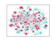
(a) ResNet-50

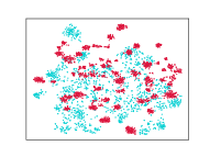
(b) DANN

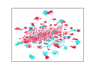
(c) BA³US

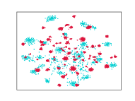
(d) LIWUDA

Figure 3: t-SNE visualizations for the transfer task Ar$\rightarrow$Cl on the Office-Home dataset under the PDA setting. Source and target instances are shown in red and blue, respectively.

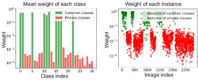
Figure 4: The average weight of each class and weights of instances in a transfer task A$\rightarrow$ W from the Office-31 dataset under the PDA setting. The green color represents instances from common classes and the red color indicates that instances are from private classes.

Table XIII: Ablation study on Office-31 dataset under the PDA setting with ResNet-50 as the backbone.

$\mathcal{L}_{\mathcal{C}}$	$\mathcal{L}_{wot}$	$\mathcal{L}_{sa}$	$\mathcal{L}_{iot}$	A$\rightarrow$W	D$\rightarrow$W	W$\rightarrow$D	A$\rightarrow$D	D$\rightarrow$A	W$\rightarrow$A	Avg
$\surd$				75.59$\pm$1.09	96.27$\pm$0.85	98.09$\pm$0.74	83.44$\pm$1.12	83.92$\pm$0.95	84.97$\pm$0.86	87.05
$\surd$	$\surd$			99.52$\pm$ 0.31	99.13$\pm$0.21	100.00$\pm$0.00	$99.42\pm$ 0.13	94.78$\pm$0.25	95.02$\pm$ 0.20	97.98
$\surd$	$\surd$	$\surd$		99.67$\pm$ 0.26	100.00$\pm$0.00	100.00$\pm$0.00	100.00$\pm$0.00	95.00$\pm$0.16	95.72$\pm$0.21	98.40
$\surd$	$\surd$	$\surd$	$\surd$	99.71$\pm$0.10	100.00$\pm$0.00	100.00$\pm$0.00	99.42$\pm$0.12	96.33$\pm$0.15	96.62$\pm$0.10	98.68

Table XIV: Ablation study on the Office-Home dataset under the PDA setting with ResNet-50 as the backbone.

$\mathcal{L}_{\mathcal{C}}$	$\mathcal{L}_{wot}$	$\mathcal{L}_{sa}$	$\mathcal{L}_{iot}$	Ar$\rightarrow$Cl	Ar$\rightarrow$Pr	Ar$\rightarrow$Rw	Cl$\rightarrow$Ar	Cl$\rightarrow$Pr	Cl$\rightarrow$Rw	Pr$\rightarrow$Ar	Pr$\rightarrow$Cl	Pr$\rightarrow$Rw	Rw$\rightarrow$Ar	Rw$\rightarrow$Cl	Rw$\rightarrow$Pr	Avg
$\surd$				46.33	67.51	75.87	59.14	59.94	62.73	58.22	41.79	74.88	67.40	48.18	74.17	61.35
$\surd$	$\surd$			58.63	79.64	83.10	67.40	68.46	76.42	75.48	57.73	82.33	83.10	65.97	84.09	73.53
$\surd$	$\surd$	$\surd$		60.06	79.05	84.48	67.49	69.13	77.03	76.03	64.12	82.77	81.91	68.03	84.43	74.55
$\surd$	$\surd$	$\surd$	$\surd$	62.15$\pm$0.15	84.59$\pm$0.15	85.48 $\pm$0.14	71.17$\pm$0.13	74.34$\pm$0.13	80.89$\pm$0.16	78.15$\pm$0.11	64.72$\pm$0.21	84.65$\pm$0.24	82.60$\pm$0.12	69.43$\pm$0.23	87.5$\pm$0.18	77.14

IV-D Sensitivity Analysis

In this section, our experimentation aims to gauge the sensitivity of the performance of the LIWUDA method in relation to its hyperparameters (i.e., $\beta$, $\eta$, and $\epsilon$). The ensuing results are presented in Tables X, XI, and XII, wherein the sets of potential values for these hyperparameters are defined as $\{0,0.05,0.1,0.2,0.5\}$, $\{0,0.1,0.2,0.3,0.4,0.5\}$, and $\{0,0.05,0.1,0.2\}$, correspondingly. The analysis reveals that performance associated with non-zero hyperparameter values consistently outpaces that linked to zero hyperparameter values, thereby underscoring the effectiveness of the proposed loss functions embedded within the LIWUDA method. Additionally, the pinnacle of performance materializes when $\beta$, $\eta$, and $\epsilon$ are respectively set to 0.1, 0.3, and 0.05. Consequently, these settings are embraced across all experiments to ensure optimal performance across all UDA scenarios.

IV-E Analysis on Weights of Instances

To substantiate the effectiveness of instance weighting within the proposed LIWUDA method, we undertake an experiment on the transfer task A$\rightarrow$ W using the Office-31 dataset within the PDA setting. The obtained results are visualized in Figure 4, illustrating the weights assigned to individual samples as well as the mean weights attributed to samples belonging to the same class within the source domain. From the insights gleaned in Figure 4, it can be observed the weights acquired through the proposed LIWUDA method aptly segregate instances from both common and private classes. This demonstrates the effectiveness of the weight network embedded within the LIWUDA framework, substantiating its role in effectively distinguishing common and private classes.

IV-F Feature Visualization

The visualization presented in Figure 3 portrays the feature representations acquired by ResNet-50 [1], DANN [56], BA³US [59], and LIWUDA on the transfer task Ar $\rightarrow$ Cl from the Office-Home dataset under the PDA setting. This visualization is facilitated through the t-SNE method [66]. Comparative analysis against baseline methods reveals a notable prowess of the proposed LIWUDA method. It demonstrates an impressive ability to align data from the same class across diverse domains, while concurrently separating data from distinct classes. This result serves as a visual testament to the capability of the LIWUDA model to adeptly align two domains under disparate label spaces in this task. This alignment factor, to some extent, contributes to the noteworthy performance exhibited by the LIWUDA method.

IV-G Ablation Study

To evaluate the individual contributions of $\mathcal{L}_{wot}$, $\mathcal{L}_{sa}$, and $\mathcal{L}_{iot}$, respectively, we train the LIWUDA model with various combinations of these losses under the PDA setting. The results are presented on Office-31 and Office-Home datasets, as detailed in Tables XIII and XIV. According to the results, even without the SA loss $\mathcal{L}_{sa}$ and IOT loss $\mathcal{L}_{iot}$, the WOT loss $\mathcal{L}_{wot}$ still achieves impressive results of 97.98% and 73.53% on the Office-31 and Office-Home datasets, showcasing the effectiveness of the WOT $\mathcal{L}_{wot}$. Furthermore, the inclusion of the SA loss ($\mathcal{L}_{sa}$) leads to a notable improvement in classification performance by 0.42% and 1.02% on the Office-31 and Office-Home datasets, affirming its effectiveness. When comparing models with or without the IOT loss ($\mathcal{L}_{iot}$), our method demonstrates a substantial increase by 0.28% and 2.59% separately. These results underscore the significant contribution of the SA loss ($\mathcal{L}_{sa}$) in separating/aligning samples, while the IOT loss ($\mathcal{L}_{iot}$) aids in achieving similar weights for common classes. In summary, the comprehensive LIWUDA method demonstrates a substantial performance boost, underscoring the synergistic effectiveness of the integrated three losses.

V Conclusion

In this work, we propose the LIWUDA method, a unified framework tailored for four distinct UDA settings accomplished through the strategic application of instance weighting. Specifically, we introduce the WOT to mitigate the domain divergence by alleviating the negative transfer caused by domain-specific classes. Additionally, we introduce the SA loss to effectively separate instances with low similarities and align instances that exhibit high similarities. To enhance the learning process of the weight network, we incorporate IOT, thereby providing supplementary insights. The integration of these three components results in the comprehensive LIWUDA framework for all four UDA settings and yields competitive performance across three benchmark datasets.

While the proposed LIWUDA method is specifically designed for UDA settings, its applicability is limited to this domain. In future work, we aim to extend the LIWUDA method to handle other settings in domain adaptation and transfer learning, such as semi-supervised domain adaptation, multi-source domain adaptation, and source-free domain adaptation.

References

- [1] K. He, X. Zhang, S. Ren, and J. Sun, “Deep residual learning for image recognition,” in 2016 IEEE Conference on Computer Vision and Pattern Recognition, CVPR. IEEE Computer Society, 2016, pp. 770–778.
- [2] S. Ren, K. He, R. B. Girshick, and J. Sun, “Faster R-CNN: towards real-time object detection with region proposal networks,” in Advances in Neural Information Processing Systems 28: Annual Conference on Neural Information Processing Systems, 2015, pp. 91–99.
- [3] J. Long, E. Shelhamer, and T. Darrell, “Fully convolutional networks for semantic segmentation,” in IEEE Conference on Computer Vision and Pattern Recognition, CVPR 2015. IEEE Computer Society, 2015, pp. 3431–3440.
- [4] Q. Yang, Y. Zhang, W. Dai, and S. J. Pan, Transfer learning. Cambridge University Press, 2020.
- [5] F. Yuan, L. Yao, and B. Benatallah, “Darec: Deep domain adaptation for cross-domain recommendation via transferring rating patterns,” in Proceedings of the Twenty-Eighth International Joint Conference on Artificial Intelligence, IJCAI 2019, Macao, China, August 10-16, 2019, S. Kraus, Ed. ijcai.org, 2019, pp. 4227–4233.
- [6] J. Deng, Z. Zhang, F. Eyben, and B. W. Schuller, “Autoencoder-based unsupervised domain adaptation for speech emotion recognition,” IEEE Signal Process. Lett., vol. 21, no. 9, pp. 1068–1072, 2014.
- [7] Y. Zou, Z. Yu, B. V. K. V. Kumar, and J. Wang, “Unsupervised domain adaptation for semantic segmentation via class-balanced self-training,” in Computer Vision - ECCV 2018 - 15th European Conference, Munich, Germany, September 8-14, 2018, Proceedings, Part III, ser. Lecture Notes in Computer Science, vol. 11207. Springer, 2018, pp. 297–313.
- [8] X. Zheng, J. Zhu, Y. Liu, Z. Cao, C. Fu, and L. Wang, “Both style and distortion matter: Dual-path unsupervised domain adaptation for panoramic semantic segmentation,” in Proceedings of the IEEE/CVF Conference on Computer Vision and Pattern Recognition, 2023, pp. 1285–1295.
- [9] J. Zhu, H. Bai, and L. Wang, “Patch-mix transformer for unsupervised domain adaptation: A game perspective,” in Proceedings of the IEEE/CVF Conference on Computer Vision and Pattern Recognition, 2023, pp. 3561–3571.
- [10] Z. Cao, L. Ma, M. Long, and J. Wang, “Partial adversarial domain adaptation,” in Computer Vision - ECCV 2018 - 15th European Conference, ser. Lecture Notes in Computer Science, vol. 11212. Springer, 2018, pp. 139–155.
- [11] P. Guo, J. Zhu, and Y. Zhang, “Selective partial domain adaptation.” in BMVC, 2022, p. 420.
- [12] K. Saito, S. Yamamoto, Y. Ushiku, and T. Harada, “Open set domain adaptation by backpropagation,” in Computer Vision - ECCV 2018 - 15th European Conference, ser. Lecture Notes in Computer Science, V. Ferrari, M. Hebert, C. Sminchisescu, and Y. Weiss, Eds., vol. 11209, 2018, pp. 156–171.
- [13] K. You, M. Long, Z. Cao, J. Wang, and M. I. Jordan, “Universal domain adaptation,” in IEEE Conference on Computer Vision and Pattern Recognition, CVPR. Computer Vision Foundation / IEEE, 2019, pp. 2720–2729.
- [14] M. Long, Y. Cao, J. Wang, and M. I. Jordan, “Learning transferable features with deep adaptation networks,” in Proceedings of the 32nd International Conference on Machine Learning, ser. JMLR Workshop and Conference Proceedings, vol. 37. JMLR.org, 2015, pp. 97–105.
- [15] M. Long, H. Zhu, J. Wang, and M. I. Jordan, “Deep transfer learning with joint adaptation networks,” in Proceedings of the 34th International Conference on Machine Learning, ICML, ser. Proceedings of Machine Learning Research, vol. 70. PMLR, 2017, pp. 2208–2217.
- [16] W. Zellinger, T. Grubinger, E. Lughofer, T. Natschläger, and S. Saminger-Platz, “Central moment discrepancy (CMD) for domain-invariant representation learning,” in 5th International Conference on Learning Representations, ICLR. OpenReview.net, 2017.
- [17] B. Sun and K. Saenko, “Deep CORAL: correlation alignment for deep domain adaptation,” in Computer Vision - ECCV 2016 Workshops - Amsterdam, The Netherlands, October 8-10 and 15-16, 2016, Proceedings, Part III, ser. Lecture Notes in Computer Science, vol. 9915, 2016, pp. 443–450.
- [18] Y. Ganin, E. Ustinova, H. Ajakan, P. Germain, H. Larochelle, F. Laviolette, M. Marchand, and V. S. Lempitsky, “Domain-adversarial training of neural networks,” J. Mach. Learn. Res., vol. 17, pp. 59:1–59:35, 2016.
- [19] J. Hoffman, E. Tzeng, T. Park, J. Zhu, P. Isola, K. Saenko, A. A. Efros, and T. Darrell, “Cycada: Cycle-consistent adversarial domain adaptation,” in Proceedings of the 35th International Conference on Machine Learning, ICML, ser. Proceedings of Machine Learning Research, vol. 80. PMLR, 2018, pp. 1994–2003.
- [20] Z. Cao, L. Ma, M. Long, and J. Wang, “Partial adversarial domain adaptation,” in Proceedings of the European Conference on Computer Vision (ECCV), 2018, pp. 135–150.
- [21] J. Zhang, Z. Ding, W. Li, and P. Ogunbona, “Importance weighted adversarial nets for partial domain adaptation,” in 2018 IEEE Conference on Computer Vision and Pattern Recognition, CVPR. Computer Vision Foundation / IEEE Computer Society, 2018, pp. 8156–8164.
- [22] Z. Cao, M. Long, J. Wang, and M. I. Jordan, “Partial transfer learning with selective adversarial networks,” in 2018 IEEE Conference on Computer Vision and Pattern Recognition, CVPR 2018. Computer Vision Foundation / IEEE Computer Society, 2018, pp. 2724–2732.
- [23] Z. Cao, K. You, M. Long, J. Wang, and Q. Yang, “Learning to transfer examples for partial domain adaptation,” in IEEE Conference on Computer Vision and Pattern Recognition, CVPR. Computer Vision Foundation / IEEE, 2019, pp. 2985–2994.
- [24] S. Li, C. H. Liu, Q. Lin, Q. Wen, L. Su, G. Huang, and Z. Ding, “Deep residual correction network for partial domain adaptation,” IEEE Trans. Pattern Anal. Mach. Intell., vol. 43, no. 7, pp. 2329–2344, 2021.
- [25] S. Bucci, M. R. Loghmani, and T. Tommasi, “On the effectiveness of image rotation for open set domain adaptation,” in Computer Vision - ECCV 2020 - 16th European Conference, ser. Lecture Notes in Computer Science, vol. 12361. Springer, 2020, pp. 422–438.
- [26] B. Fu, Z. Cao, M. Long, and J. Wang, “Learning to detect open classes for universal domain adaptation,” in Computer Vision - ECCV 2020 - 16th European Conference, ser. Lecture Notes in Computer Science, vol. 12360. Springer, 2020, pp. 567–583.
- [27] K. Saito, D. Kim, S. Sclaroff, and K. Saenko, “Universal domain adaptation through self supervision,” in Advances in Neural Information Processing Systems 33: Annual Conference on Neural Information Processing Systems 2020, NeurIPS 2020, 2020.
- [28] L. V. Kantorovich, “On the translocation of masses,” Journal of mathematical sciences, vol. 133, no. 4, pp. 1381–1382, 2006.
- [29] N. Courty, R. Flamary, D. Tuia, and A. Rakotomamonjy, “Optimal transport for domain adaptation,” IEEE Trans. Pattern Anal. Mach. Intell., vol. 39, no. 9, pp. 1853–1865, 2017.
- [30] N. Courty, R. Flamary, A. Habrard, and A. Rakotomamonjy, “Joint distribution optimal transportation for domain adaptation,” in NIPS, 2017.
- [31] I. Redko, A. Habrard, and M. Sebban, “Theoretical analysis of domain adaptation with optimal transport,” ArXiv, vol. abs/1610.04420, 2016.
- [32] I. Redko, N. Courty, R. Flamary, and D. Tuia, “Optimal transport for multi-source domain adaptation under target shift,” in International Conference on Artificial Intelligence and Statistics, 2018.
- [33] Y. Yan, W. Li, H. Wu, H. Min, M. Tan, and Q. Wu, “Semi-supervised optimal transport for heterogeneous domain adaptation,” in International Joint Conference on Artificial Intelligence, 2018.
- [34] B. Xu, Z. Zeng, C. Lian, and Z. Ding, “Few-shot domain adaptation via mixup optimal transport,” IEEE Transactions on Image Processing, vol. 31, pp. 2518–2528, 2022.
- [35] I. Redko, A. Habrard, and M. Sebban, “Theoretical analysis of domain adaptation with optimal transport,” in Machine Learning and Knowledge Discovery in Databases: European Conference, ECML PKDD 2017, Skopje, Macedonia, September 18–22, 2017, Proceedings, Part II 10. Springer, 2017, pp. 737–753.
- [36] B. B. Damodaran, B. Kellenberger, R. Flamary, D. Tuia, and N. Courty, “Deepjdot: Deep joint distribution optimal transport for unsupervised domain adaptation,” in Computer Vision - ECCV 2018 - 15th European Conference, ser. Lecture Notes in Computer Science, vol. 11208. Springer, 2018, pp. 467–483.
- [37] R. Xu, P. Liu, L. Wang, C. Chen, and J. Wang, “Reliable weighted optimal transport for unsupervised domain adaptation,” in Proceedings of the IEEE/CVF Conference on Computer Vision and Pattern Recognition, CVPR. Computer Vision Foundation / IEEE, 2020, pp. 4393–4402.
- [38] J. Shen, Y. Qu, W. Zhang, and Y. Yu, “Wasserstein distance guided representation learning for domain adaptation,” in Proceedings of the AAAI Conference on Artificial Intelligence, vol. 32, no. 1, 2018.
- [39] K. Fatras, T. S’ejourn’e, N. Courty, and R. Flamary, “Unbalanced minibatch optimal transport; applications to domain adaptation,” ArXiv, vol. abs/2103.03606, 2021.
- [40] N. Courty, R. Flamary, and D. Tuia, “Domain adaptation with regularized optimal transport,” in Machine Learning and Knowledge Discovery in Databases: European Conference, ECML PKDD 2014, Nancy, France, September 15-19, 2014. Proceedings, Part I 14. Springer, 2014, pp. 274–289.
- [41] C.-Y. Lee, T. Batra, M. H. Baig, and D. Ulbricht, “Sliced wasserstein discrepancy for unsupervised domain adaptation,” in Proceedings of the IEEE/CVF conference on computer vision and pattern recognition, 2019, pp. 10 285–10 295.
- [42] R. Xu, P. Liu, Y. Zhang, F. Cai, J. Wang, S. Liang, H. Ying, and J. Yin, “Joint partial optimal transport for open set domain adaptation.” in IJCAI, 2020, pp. 2540–2546.
- [43] B. Colson, P. Marcotte, and G. Savard, “An overview of bilevel optimization,” Ann. Oper. Res., vol. 153, no. 1, pp. 235–256, 2007.
- [44] L. A. Caffarelli and R. J. McCann, “Free boundaries in optimal transport and monge-ampere obstacle problems,” Annals of mathematics, pp. 673–730, 2010.
- [45] L. Chapel, M. Z. Alaya, and G. Gasso, “Partial optimal transport with applications on positive-unlabeled learning,” arXiv preprint arXiv:2002.08276, 2020.
- [46] K. Nguyen, D. Nguyen, T. Pham, N. Ho et al., “Improving mini-batch optimal transport via partial transportation,” in International Conference on Machine Learning. PMLR, 2022, pp. 16 656–16 690.
- [47] I. Redko, A. Habrard, and M. Sebban, “Theoretical analysis of domain adaptation with optimal transport,” in Machine Learning and Knowledge Discovery in Databases - European Conference, ECML PKDD 2017, ser. Lecture Notes in Computer Science, vol. 10535, 2017, pp. 737–753.
- [48] K. Saenko, B. Kulis, M. Fritz, and T. Darrell, “Adapting visual category models to new domains,” in Computer Vision - ECCV 2010, 11th European Conference on Computer Vision, ser. Lecture Notes in Computer Science, vol. 6314. Springer, 2010, pp. 213–226.
- [49] H. Venkateswara, J. Eusebio, S. Chakraborty, and S. Panchanathan, “Deep hashing network for unsupervised domain adaptation,” in 2017 IEEE Conference on Computer Vision and Pattern Recognition, CVPR 2017. IEEE Computer Society, 2017, pp. 5385–5394.
- [50] X. Peng, B. Usman, N. Kaushik, J. Hoffman, D. Wang, and K. Saenko, “Visda: The visual domain adaptation challenge,” CoRR, vol. abs/1710.06924, 2017.
- [51] H. Liu, Z. Cao, M. Long, J. Wang, and Q. Yang, “Separate to adapt: Open set domain adaptation via progressive separation,” in IEEE Conference on Computer Vision and Pattern Recognition, CVPR. Computer Vision Foundation / IEEE, 2019, pp. 2927–2936.
- [52] S. Li, C. H. Liu, Q. Lin, Q. Wen, L. Su, G. Huang, and Z. Ding, “Deep residual correction network for partial domain adaptation,” IEEE Trans. Pattern Anal. Mach. Intell., vol. 43, no. 7, pp. 2329–2344, 2021.
- [53] P. P. Busto, A. Iqbal, and J. Gall, “Open set domain adaptation for image and action recognition,” IEEE Trans. Pattern Anal. Mach. Intell., vol. 42, no. 2, pp. 413–429, 2020.
- [54] M. Long, H. Zhu, J. Wang, and M. I. Jordan, “Unsupervised domain adaptation with residual transfer networks,” in Advances in Neural Information Processing Systems 29: Annual Conference on Neural Information Processing Systems 2016, 2016, pp. 136–144.
- [55] M. Long, Y. Cao, J. Wang, and M. I. Jordan, “Learning transferable features with deep adaptation networks,” in Proceedings of the 32nd International Conference on Machine Learning, ICML 2015, Lille, France, 6-11 July 2015, ser. JMLR Workshop and Conference Proceedings, vol. 37. JMLR.org, 2015, pp. 97–105.
- [56] Y. Ganin, E. Ustinova, H. Ajakan, P. Germain, H. Larochelle, F. Laviolette, M. Marchand, and V. Lempitsky, “Domain-adversarial training of neural networks,” The journal of machine learning research, vol. 17, no. 1, pp. 2096–2030, 2016.
- [57] E. Tzeng, J. Hoffman, K. Saenko, and T. Darrell, “Adversarial discriminative domain adaptation,” in 2017 IEEE Conference on Computer Vision and Pattern Recognition, CVPR. IEEE Computer Society, 2017, pp. 2962–2971.
- [58] Z. Chen, C. Chen, Z. Cheng, B. Jiang, K. Fang, and X. Jin, “Selective transfer with reinforced transfer network for partial domain adaptation,” in 2020 IEEE/CVF Conference on Computer Vision and Pattern Recognition, CVPR. Computer Vision Foundation / IEEE, 2020, pp. 12 703–12 711.
- [59] J. Liang, Y. Wang, D. Hu, R. He, and J. Feng, “A balanced and uncertainty-aware approach for partial domain adaptation,” in Computer Vision–ECCV 2020: 16th European Conference. Springer, 2020, pp. 123–140.
- [60] G. Li, G. Kang, Y. Zhu, Y. Wei, and Y. Yang, “Domain consensus clustering for universal domain adaptation,” in Proceedings of the IEEE/CVF Conference on Computer Vision and Pattern Recognition, 2021, pp. 9757–9766.
- [61] K. Simonyan and A. Zisserman, “Very deep convolutional networks for large-scale image recognition,” in 3rd International Conference on Learning Representations, ICLR, 2015.
- [62] J. N. Kundu, N. Venkat, R. M. V., and R. V. Babu, “Universal source-free domain adaptation,” in Proceedings of the IEEE/CVF Conference on Computer Vision and Pattern Recognition, CVPR. Computer Vision Foundation / IEEE, 2020, pp. 4543–4552.
- [63] L. P. Jain, W. J. Scheirer, and T. E. Boult, “Multi-class open set recognition using probability of inclusion,” in Computer Vision - ECCV 2014 - 13th European Conference, ser. Lecture Notes in Computer Science, vol. 8691. Springer, 2014, pp. 393–409.
- [64] E. Tzeng, J. Hoffman, N. Zhang, K. Saenko, and T. Darrell, “Deep domain confusion: Maximizing for domain invariance,” CoRR, vol. abs/1412.3474, 2014.
- [65] Y. Ganin and V. S. Lempitsky, “Unsupervised domain adaptation by backpropagation,” in Proceedings of the 32nd International Conference on Machine Learning, ICML, ser. JMLR Workshop and Conference Proceedings, vol. 37. JMLR.org, 2015, pp. 1180–1189.
- [66] J. Donahue, Y. Jia, O. Vinyals, J. Hoffman, N. Zhang, E. Tzeng, and T. Darrell, “Decaf: A deep convolutional activation feature for generic visual recognition,” in Proceedings of the 31th International Conference on Machine Learning, ICML, ser. JMLR Workshop and Conference Proceedings, vol. 32. JMLR.org, 2014, pp. 647–655.